DEPARTMENT OF STATISTICSUniversity of Wisconsin1300 University Ave.Madison, WI 53706

TECHNICAL REPORT NO. 1179June 4, 2015

Statistical Justifications for Computationally Tractable

Network Data Analysis

Tai Qin

1

Department of Statistics

University of Wisconsin, Madison

1Research of TQ is supported by NSF Grant DMS1308877.

STATISTICAL JUSTIFICATIONS FOR COMPUTATIONALLY

TRACTABLE NETWORK DATA ANALYSIS

by

Tai Qin

A dissertation submitted in partial fulfillment of

the requirements for the degree of

Doctor of Philosophy

(Statistics)

at the

UNIVERSITY OF WISCONSIN–MADISON

2015

Date of final oral examination: 05/15/2015

The dissertation is approved by the following members of the Final Oral Committee:

Grace Wahba, IJ Schoenberg-Hilldale Professor, Statistics

Karl Rohe, Assistant Professor, Statistics

Ming Yuan, Professor, Statistics

Sushmita Roy, Assistant Professor, Biostatistics

Xiaojin Zhu, Associate Professor, Computer Science

c� Copyright by Tai Qin 2015All Rights Reserved

i

To my wife Yi Fan, and parents Hanghui Li and Jianren Qin

ii

Abstract

Our lives are embedded in networks. Many researchers wish to analyze these networksto gain a deeper understanding of the underlying mechanisms. Some types ofunderlying mechanisms generate communities (aka clusters or modularities) in thenetwork. This work aims not merely to devise algorithms for community detection,but also to study the algorithms’ estimation properties, to understand if and whenwe can make justifiable inferences from the estimated communities to the underlyingmechanisms.

Spectral clustering is a popular algorithm for community detection. Yet it failswhen dealing with networks with degree heterogeneity. Chapter 2 proposes regularizedspectral clustering and extends the previous statistical estimation results (Chaudhuriet al. (2012) and Amini et al. (2012)) to the more canonical spectral clusteringalgorithm in a way that removes any assumption on the minimum degree andprovides guidance on the choice of the tuning parameter. Moreover, our results showhow the “star shape” in the eigenvectors – a common feature of empirical networks –can be explained by the Degree-Corrected Stochastic Blockmodel and the ExtendedPlanted Partition model, two statistical models that allow for highly heterogeneousdegrees.

Chapter 3 extends the regularized spectral clustering algorithm to directed net-works with general degrees. Chapter 3 proposes and studies a spectral co-clusteringalgorithm called di-sim. Building on previous spectral co-clustering algorithms (e.g.Dhillon (2001)), di-sim incorporates regularization and projection steps. We showthat these two steps are essential when there is a large amount of degree heterogeneityand several weakly connected nodes.

Chapter 4 studies a random network model where, ignoring log terms, number ofclusters (or communities) K can grow proportionally to number of nodes N . Since thenumber of clusters must be smaller than the number of nodes, no reasonable modelallows K to grow faster; thus, our asymptotic results are the “highest” dimensional.Furthermore, we develop a regularized maximum likelihood estimator that enjoys weakconsistency under certain conditions. This is the first work to explicitly introduce

iii

and demonstrate the advantages of statistical regularization in a parametric form fornetwork analysis.

Chapter 5 proposes a fast and memory e�cient community detection algorithm.It is built upon regularized spectral clustering and the Nystrom extension with propernormalization and regularization. We provide a bound for its misclustering rate underthe Degree-Corrected Stochastic Blockmodel.

Finally, chapter 6 studies the interaction between transitivity and sparsity. Thetwo common features in empirical networks, implies that there are local regions oflarge sparse networks that are dense. We call this the blessing of transitivity and ithas consequences for both modeling and inference. Extant research suggests thatstatistical inference for the Stochastic Blockmodel is more di�cult when the edgesare sparse. However, this conclusion is confounded by the fact that the asymptoticlimit in all of the previous studies is not merely sparse, but also non-transitive. Toretain transitivity, the blocks cannot grow faster than the expected degree. Thus, insparse models, the blocks must remain asymptotically small. Previous algorithmicresearch demonstrates that small “local” clusters are more amenable to computation,visualization, and interpretation when compared to “global” graph partitions. Thispaper provides the first statistical results that demonstrate how these small transitiveclusters are also more amenable to statistical estimation. Theorem 2 of chapter6 shows that a “local” clustering algorithm can, with high probability, detect atransitive stochastic block of a fixed size (e.g. 30 nodes) embedded in a large graph.The only constraint on the ambient graph is that it is large and sparse–it could begenerated at random or by an adversary–suggesting a theoretical explanation for therobust empirical performance of local clustering algorithms.

iv

Acknowledgments

I am blessed to have Grace and Karl as my two advisors.In my second year, I felt lost and depressed in the transition from taking classes to

doing research. Grace introduced me to the topic of spectral methods which later turnout to be the main theme of this thesis. Research requires creativity and persistence.I am grateful to Grace for giving me infinity degree of freedom for choosing researchtopics and encouraging and supporting me to go ahead on whichever road I pick.

In my mailbox, there are more than five hundred emails if searching “Karl”. Someof his emails displays sending time around 5 to 6am. Karl is always passionate andoptimistic about work and life. Some of his energy and attitude toward life passed onme, which makes me a better researcher, and a better person. He is more like a friendthan a mentor to me. May 31, 2013 was the submission deadline for a conference.We were working on it to the last minute at Karl’s home. When we finished, it wasalready about 6:30pm. I went downstairs and found his whole family waiting forhim to celebrate his little baby’s first birthday. We worked on various projects, somefailed, some turned out OK. I enjoyed all of them.

I am thankful to my thesis committee: Prof. Ming Yuan, Prof. Sushmita Royand Prof. Xiaojin (Jerry) Zhu for the helpful advices and suggestions, and moreimportantly, for letting me pass.

Thank the faculty members for teaching me classes and conversations out side ofclass. Ming knows everything in statistical theory. I am grateful to him for pushing usaiming higher and thinking deeper. Prof. Wei-Yin Loh introduced me to Kaggle. Theonline data competition platform opens a window for me to learn practical statisticalmodeling. Thank Prof. Peter Qian, Prof. Sijian Wang, Prof. Garvesh Raskutt, Prof.Jun Shao, Prof. Douglas Bates, Prof. Chunming Zhang, Prof. Zhengjun Zhang, Prof.Krishnakumar Balasubramanian and Prof. Stephen Wright.

Thank the Thursday’s group and the Friday’s group for the discussions andinspiring ideas from di↵erent prospectives. Thank Zhigeng Geng (also my reliablebadminton doubles team partner), Jing Kong, Bin Dai, Shilin Ding, Luwan Zhang,Han Chen, Shulei Wang, Hao Zhou, Yilin Zhang, Xiaowu Dai, and the Friday group:

v

Juhee Cho, Kim Donggyu, Mohammad Khabbazian, Thu Le, Norbert Binkiewicz, ZoeRussek, Nick Zaborek and Song Wang. Thank my friends, Zhishi, Haoyang, Lilun,Xu, Chandler, Yunfei, Chenliang, Jianan, Yan, Jiajie, Lu, Vincent, Lie, Yaodong andheng. Thank our small friday “practical probability theory training session”. Lifewill be bored without my friends.

At last, thank my wife Yi, for making my life tasty, in every way it can be.

vi

Contents

Abstract ii

Contents vi

List of Figures viii

1 Introduction 1

2 Regularized Spectral Clustering under the Degree-Corrected StochasticBlockmodel 32.1 Introduction 32.2 The Algorithm: Regularized Spectral Clustering (RSC) 52.3 The Degree-Corrected Stochastic Blockmodel (DC-SBM) 62.4 Regularized Spectral Clustering with the Degree-corrected model 82.5 Simulation and Analysis of Political Blogs 132.6 Discussion 16

3 Regularized Co-clustering for Directed Graphs 173.1 Introduction 173.2 The di-sim Algorithm 183.3 Stochastic co-Blockmodel 203.4 Estimating the Degree Corrected Stochastic co-Blockmodel with di-

sim 233.5 Simulation 293.6 Discussion 31

4 The Highest Dimensional Stochastic Blockmodel with a Regularized Esti-mator 344.1 Introduction 34

vii

4.2 Preliminaries 374.3 Performance of the RMLE in the highest dimensional asymptotic

setting 404.4 Simulations 424.5 Discussion 46

5 Memory E�cient Community Detection under the Degree-Corrected Stochas-tic Blockmodel 475.1 Introduction 475.2 Algorithm: Memory e�cient regularized spectral clustering(mRSC) 525.3 Population analysis 535.4 Perturbation analysis and a bound on mis-clustering rate 555.5 Discussion 58

6 The Blessing of Transitivity in Sparse and Stochastic Networks 596.1 Introduction 596.2 Transitivity in sparse exchangeable random graph models 646.3 Local ( model + algorithm + results ) 686.4 The Degree-corrected Local Stochastic Blockmodel 746.5 Discussion 79

A Appendix for Chapter 2 81

B Appendix for Chapter 3 88B.1 Convergence of Singular Vectors 88B.2 Proof of Theorem 3.7 93

C Appendix for Chapter 4 101

D Appendix for Chapter 5 109

E Appendix for Chapter 6117

References 128

viii

List of Figures

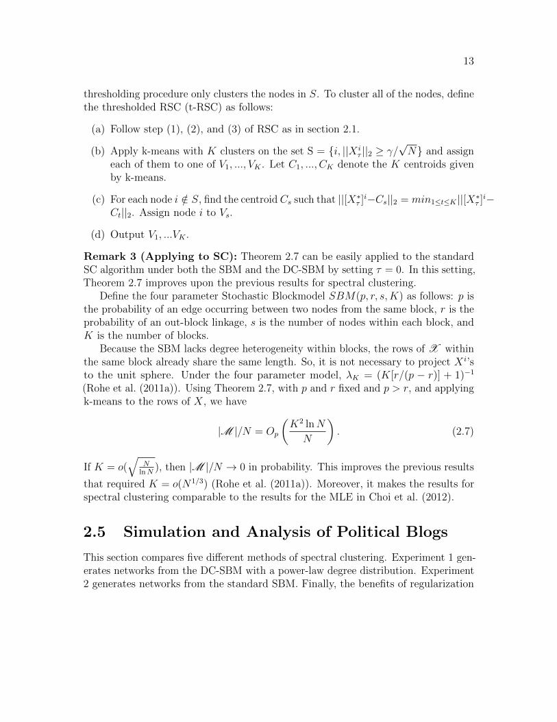
2.1 In this numerical example, A comes from the DC-SBM with three blocks.Each point corresponds to one row of the matrix X⌧ (in left panel) orX ⇤

⌧ (in right panel). The di↵erent colors correspond to three di↵erentblocks. The hollow circle is the origin. Without normalization (left panel),the nodes with same block membership share the same direction in theprojected space. After normalization (right panel), nodes with same blockmembership share the same position in the projected space. . . . . . . . 9

2.2 Left Panel: Comparison of Performance for SC, RSC, RSC wp, t-RSC,SCP and (RSC on S) under di↵erent degree heterogeneity. Smaller �corresponds to greater degree heterogeneity. Right Panel: Comparison ofPerformance for SC and RSC under SBM with di↵erent sparsity. . . . . . 15

3.1 In the simulation on the left, the data comes from the four parameterStochastic Co-Blockmodel. On the right, the data comes from the samemodel, but with degree correction. The ✓i parameters have expectationone. In both models, k = 5 and s = 400. The probabilities p and rvary such that p = 5r, keeping the spectral gap fixed at �k = 1/2. Thissimulation shows that for small expected degree, regularization decreasesthe proportion of nodes that are misclustered. Moreover, the benefits ofregularization are more pronounced under the degree corrected model. . 30

ix

3.2 In the simulation on the left, the data comes from the four parameterStochastic Co-Blockmodel. On the right, the data comes from the samemodel, but with degree correction. The ✓i parameters have expectationone. In both models, k = 5 and s = 400. The spectral gap, displayed onthe horizontal axis, changes because the probabilities p and r change. Thevalues of p and r vary in a way that keeps the expected degree fixed attwenty for all simulations. Without degree correction, the three separatelines are di�cult to distinguish because they are nearly identical. Underthe degree corrected model, regularization improves performance whenthe spectral gap is small. . . . . . . . . . . . . . . . . . . . . . . . . . . 32

4.1 In this simulation, across a wide range of K, the RMLE misclusters fewernodes than the MLE. In each simulation, every block contains 20 nodes andK grows from 10 to 100 along the horizontal axis. The vertical axis displaysthe proportion of nodes misclustered. Both algorithms are initialized withregularized spectral clustering and the results for this initialization aredisplayed by the dashed line. The MLE makes minor improvements tothe initialization, while the RMLE makes more significant improvements.Each point in this figure represents the average of 300 simulations. Allmethods were run on the same simulated adjacency matrices. . . . . . . 44

4.2 These figures investigate the sensitivity of the algorithms to deviationsfrom the RMLE’s “implied model” that has homogeneous o↵-diagonalelements in ✓. The top left figure displays results when these elementsof ✓ come from the Gamma distribution with varying shape parameter.The top right figure displays results when these elements of ✓ come fromthe Bernoulli distribution with varying probability p. In both cases, ad-justments are made so that each node has five expected out-of-blockneighbors. The bottom plots illustrate the how these heterogenous proba-bilities manifest in the adjacency matrix; in both cases, A is sampled withthe parameterization that corresponds to the break-even point between theMLE and the RMLE. Each point represents an average over 200 simulations 45

6.1 Local clusters from a sparse 76k node social network from epinions.com.Created with the igraph library in R (Csardi and Nepusz, 2006). . . . . 60

6.2 This figure illustrates the two types of triangles that contain nodes in bothS⇤ and Sc

⇤. To make one triangle that crosses the boundary of S requirestwo edges to cross the boundary. . . . . . . . . . . . . . . . . . . . . . . 72

x

6.3 This plots the number of nodes in the largest ten clusters (ignoring asingle giant cluster) found by GlobalTrans(A, cut) in the slashdot socialnetwork. These clusters are very small, and probably too small for manyapplications. Moreover, there are not that many of them. . . . . . . . . 73

6.4 A plot of the number of nodes in the largest ten clusters (ignoring onevery large cluster) found by GlobalTrans(L⌧ , cut) in the slashdot socialnetwork. GlobalTrans with L⌧ instead of A finds much larger clusters. 78

6.5 Twenty-four small clusters from the slashdot data set. Because GlobalTransdiscovers small clusters, one can easily plot and visualize the clusters witha standard graph visualization tool (Csardi and Nepusz, 2006). The pointof this figure is to show the variability in cluster structures; some aretight, clique-like clusters; others are small lattice-like clusters; others are“stringy” collections of three or four tight clusters. This highlights the easeof visualizing the results of local clustering. . . . . . . . . . . . . . . . . . 79

6.6 Starting from a seed node, this figure demonstrates how LocalTrans(L⌧=12

, i, cut)grows as cut decreases. In each panel, the graph is drawn for the smallestvalue of cut, and the solid nodes correspond to the nodes returned byLocalTrans(L⌧=12

, i, cut), where the value of cut is given above the graphin the units 10�6. Moving from left to right, the clusters grow larger, andthe additional nodes start to extend to the periphery of the visualization. 80

1

Chapter 1

Introduction

Recent advances in information technology have produced a deluge of data on complexsystems with myriad interacting elements, easily represented by networks or graphs.Communities or clusters of highly connected actors are an essential feature in amultitude of empirical networks, and identifying these clusters helps answer vitalquestions in various fields. Depending on the area of interest, interacting elementsmay be metabolites, people, or computers. Their interactions can be represented inchemical reactions, friendships, or some type of communication. For example, onFacebook, groups of people sharing same interest or attending same college formvarious communities; a terrorist cell is a cluster in the communication network ofterrorists; web pages that provide hyperlinks to each other form a community thatmay host discussions of a similar topic; a cluster in the network of biochemicalreactions might contain metabolites with similar functions and activities. Networks(or graphs) appropriately describe these relationships. Therefore, the substantivequestions in these various disciplines are, in essence, questions regarding the structureof networks. Given the demonstrated interest in making statistical inference froman observed network, it is essential to evaluate the ability of clustering algorithmsto estimate the “true clusters” in a network model. Understanding when and why aclustering algorithm correctly estimates the “true communities” provides a rigorousunderstanding of the behavior of these algorithms and potentially leads to improvedalgorithms.

Networks can be complex. Community structures are confounded with manyother features of various types of networks:

(a). In many networks, like the world wide web, their degrees are highly het-erogeneous, some approximately follow power-law distribution (Adamic andHuberman (2000)). For a sparse network with strong degree heterogeneity,

2

standard spectral clustering often fails to function properly (Amini et al. (2012);Jin (2012)).

(b). Some networks consist of small communities. Dunbar (1992) suggests thathumans do not have the social intellect to maintain stable communities largerthan roughly 150 people (colloquially referred to as Dunbar’s number). Leskovecet al. (2008) found a similar result in several other networks that were notcomposed of humans. The research of Leskovec et al. (2008) and Dunbar (1992)suggests that the community sizes should not grow asymptotically.

(c). Some networks are just too large to be even stored in computer memory forfurther analysis. In this case, it is important to find a balance point in thetradeo↵ between accuracy and computing resource.

(d). Transitivity and sparsity are two common features of many networks. Extantresearch suggests that statistical inference for the Stochastic Blockmodel ismore di�cult when the edges are sparse.

This work aims to devise and study regularized algorithms that detect communitiesunder these confounding issues with theoretical performance guarantee. Chapter2 introduces regularized spectral clustering(RSC) that improves the performancestandard spectral clustering under scenario (a). Chapter 3 extends RSC to directednetworks with degree heterogeneity. Chapter 4 studies a regularized maximumlikelihood estimator that are proven to be useful under asymptotic settings thatmimics scenario (b). Chapter 5 develops and studies a memory e�cient spectralalgorithm that deals with scenario (c). Lastly chapter 6 studies the interactionbetween transitivity and sparsity and shows that transitivity can be helpful infinding communities in sparse networks. Chapter 6 then introduces a local clusteringalgorithm that can, with high probability, detect transitive stochastic block of a fixedsize (e.g. 30 nodes) embedded in a large graph.

Each chapter, although highly related to each other, is self-contained. Readerscan start from any chapters of interests. Chapter 2 is adapted from Qin and Rohe(2013a). Chapter 3 is largely adapted from Rohe, Qin, and Yu (2015). Chapter 4 isadapted from Rohe, Qin, and Fan (2014). Chapter 6 is adapted from Rohe and Qin(2013).

3

Chapter 2

Regularized Spectral Clusteringunder the Degree-CorrectedStochastic Blockmodel

2.1 Introduction

Spectral clustering is a fast and popular algorithm for finding clusters in networks.Recently, Chaudhuri et al. (2012) and Amini et al. (2012) proposed inspired variationson the algorithm that artificially inflate the node degrees for improved statisticalperformance. This chapter extends the previous statistical estimation results to themore canonical spectral clustering algorithm in a way that removes any assumptionon the minimum degree and provides guidance on the choice of the tuning parameter.Moreover, our results show how the “star shape” in the eigenvectors – a commonfeature of empirical networks – can be explained by the Degree-Corrected StochasticBlockmodel and the Extended Planted Partition model, two statistical models thatallow for highly heterogeneous degrees. Throughout, this chapter characterizes andjustifies several of the variations of the spectral clustering algorithm in terms of thesemodels.

Several previous authors have studied the estimation properties of spectral clus-tering under various statistical network models (McSherry (2001); Dasgupta et al.(2004); Coja-Oghlan and Lanka (2009); Ames and Vavasis (2010); Rohe et al. (2011a);Sussman et al. (2012b) and Chaudhuri et al. (2012)). Recently, Chaudhuri et al.(2012) and Amini et al. (2012) proposed two inspired ways of artificially inflating thenode degrees in ways that provide statistical regularization to spectral clustering.

This chapter examines the statistical estimation performance of regularized spectral

4

clustering under the Degree-Corrected Stochastic Blockmodel (DC-SBM), an extensionof the Stochastic Blockmodel (SBM) that allows for heterogeneous degrees (Hollandand Leinhardt (1983); Karrer and Newman (2011)). The SBM and the DC-SBM areclosely related to the planted partition model and the extended planted partitionmodel, respectively. We extend the previous results in the following ways:

(a) In contrast to previous studies, this paper studies the regularization step witha canonical version of spectral clustering that uses k-means. The results do notrequire any assumptions on the minimum expected node degree; instead, thereis a threshold demonstrating that higher degree nodes are easier to cluster. Thisthreshold is a function of the leverage scores that have proven essential in othercontexts, for both graph algorithms and network data analysis (see Mahoney(2012a) and references therein). These are the first results that relate leveragescores to the statistical performance of spectral clustering.

(b) This paper provides more guidance for data analytic issues than previousapproaches. First, the results suggest an appropriate range for the regularizationparameter. Second, our analysis gives a (statistical) model-based explanationfor the “star-shaped” figure that often appears in empirical eigenvectors. Thisdemonstrates how projecting the rows of the eigenvector matrix onto the unitsphere (an algorithmic step proposed by Ng et al. (2002)) removes the ancillarye↵ects of heterogeneous degrees under the DC-SBM. Our results highlight whenthis step may be unwise.

Preliminaries: Throughout, we study undirected and unweighted graphs ornetworks. Define a graph as G(E, V ), where V = {v

1

, v2

, . . . , vN} is the vertex ornode set and E is the edge set. We will refer to node vi as node i. E contains a pair(i, j) if there is an edge between node i and j. The edge set can be represented bythe adjacency matrix A 2 {0, 1}n⇥n. Aij = Aji = 1 if (i, j) is in the edge set andAij = Aji = 0 otherwise. Define the diagonal matrix D and the normalized GraphLaplacian L, both elements of RN⇥N , in the following way:

Dii =X

j

Aij, L = D�1/2AD�1/2.

The following notations will be used throughout the paper: || · || denotes thespectral norm, and || · ||F denotes the Frobenius norm. For two sequence of variables{xN} and {yN}, we say xN = !(yN ) if and only if yN/xN = o(1). �

(.,.) is the indicatorfunction where �x,y = 1 if x = y and �x,y = 0 if x 6= y.

5

2.2 The Algorithm: Regularized SpectralClustering (RSC)

For a sparse network with strong degree heterogeneity, standard spectral clusteringoften fails to function properly (Amini et al. (2012); Jin (2012)). To account for this,Chaudhuri et al. (2012) proposed the regularized graph Laplacian that can be definedas

L⌧ = D�1/2⌧ AD�1/2

⌧ 2 RN⇥N

where D⌧ = D + ⌧I for ⌧ � 0.The spectral algorithm proposed and studied by Chaudhuri et al. (2012) divides

the nodes into two random subsets and only uses the induced subgraph on one ofthose random subsets to compute the spectral decomposition. In this paper, wewill study the more traditional version of spectral algorithm that uses the spectraldecomposition on the entire matrix (Ng et al. (2002)). Define the regularized spectralclustering (RSC) algorithm as follows:

RSC

Input: Adjacency matrix A 2 {0, 1}n⇥n, regularizer ⌧ � 0 (Default: ⌧ = averagenode degree), number of clusters K.

1. Given input adjacency matrix A, number of clusters K, and regularizer ⌧ ,calculate the regularized graph Laplacian L⌧ . (As discussed later, a gooddefault for ⌧ is the average node degree.)

2. Find the eigenvectors X1

, ..., XK 2 RN corresponding to the K largest eigen-values of L⌧ . Form X = [X

1

, ..., XK ] 2 RN⇥K by putting the eigenvectorsinto the columns.

3. Form the matrix X⇤ 2 RN⇥K from X by normalizing each of X’s rows tohave unit length. That is, project each row of X onto the unit sphere of RK

(X⇤ij = Xij/(

P

j X2

ij)1/2).

4. Treat each row of X⇤ as a point in RK , and run k-means with K clusters.This creates K non-overlapping sets V

1

, ..., VK whose union is V.

5. Node i is assigned to cluster r if the i’th row of X⇤ is assigned to Vr.

Output: The clusters V1

, ..., VK from step (5).

6

This paper will refer to “standard spectral clustering” as the above algorithmwith L replacing L⌧ .

These spectral algorithms have two main steps: 1) find the principal eigenspace ofthe (regularized) graph Laplacian; 2) determine the clusters in the low dimensionaleigenspace. Later, we will study RSC under the Degree-Corrected Stochastic Block-model and show rigorously how regularization helps to maintain cluster informationin step (a) and why normalizing the rows of X helps in step (b). From now on, weuse X⌧ and X⇤

⌧ instead of X and X⇤ to emphasize that they are related to L⌧ . LetX i

⌧ and [X⇤⌧ ]

i denote the i’th row of X⌧ and X⇤⌧ .

The next section introduces the Degree-Corrected Stochastic Blockmodel and itsmatrix formulation.

2.3 The Degree-Corrected StochasticBlockmodel (DC-SBM)

In the Stochastic Blockmodel (SBM), each node belongs to one of K blocks. Eachedge corresponds to an independent Bernoulli random variable where the probabilityof an edge between any two nodes depends only on the block memberships of the twonodes (Holland and Leinhardt (1983)). The formal definition is as follows.

Definition 2.1. For a node set {1, 2, ..., N}, let z : {1, 2, ..., N} ! {1, 2, ..., K}partition the N nodes into K blocks. So, zi equals the block membership for node i.Let B be a K ⇥K matrix where Bab 2 [0, 1] for all a, b. Then under the SBM, theprobability of an edge between i and j is Pij = Pji = Bz

i

zj

for any i, j = 1, 2, ..., n.Given z, all edges are independent.

One limitation of the SBM is that it presumes all nodes within the same block havethe same expected degree. The Degree-Corrected Stochastic Blockmodel (DC-SBM)(Karrer and Newman (2011)) is a generalization of the SBM that adds an additionalset of parameters (✓i > 0 for each node i) that control the node degrees. Let Bbe a K ⇥ K matrix where Bab � 0 for all a, b. Then the probability of an edgebetween node i and node j is ✓i✓jBz

i

zj

, where ✓i✓jBzi

zj

2 [0, 1] for any i, j = 1, 2, ..., n.Parameters ✓i are arbitrary to within a multiplicative constant that is absorbedinto B. To make it identifiable, Karrer and Newman (2011) suggest imposing theconstraint that, within each block, the summation of ✓i’s is 1. That is,

P

i ✓i�zi,r = 1for any block label r. Under this constraint, B has explicit meaning: If s 6= t, Bst

represents the expected number of links between block s and block t and if s = t,

7

Bst is twice the expected number of links within block s. Throughout the paper, weassume that B is positive definite.

Under the DC-SBM, define A , EA. This matrix can be expressed as a productof the matrices,

A = ⇥ZBZT⇥,

where (1) ⇥ 2 RN⇥N is a diagonal matrix whose ii’th element is ✓i and (2) Z 2{0, 1}N⇥K is the membership matrix with Zit = 1 if and only if node i belongs toblock t (i.e. zi = t).

Population Analysis

Under the DC-SBM, if the partition is identifiable, then one should be able todetermine the partition from A . This section shows that with the populationadjacency matrix A and a proper regularizer ⌧ , RSC perfectly reconstructs the blockpartition.

Define the diagonal matrix D to contain the expected node degrees, Dii =P

j Aij

and define D⌧ = D + ⌧I where ⌧ � 0 is the regularizer. Then, define the populationgraph Laplacian L and the population version of regularized graph Laplacian L⌧ ,both elements of RN⇥N , in the following way:

L = D�1/2A D�1/2, L⌧ = D�1/2⌧ A D�1/2

⌧ .

DefineDB 2 RK⇥K as a diagonal matrix whose (s, s)’th element is [DB]ss =P

t Bst.A couple lines of algebra shows that [DB]ss = Ws is the total expected degrees ofnodes from block s and that Dii = ✓i[DB]z

i

zi

. Using these quantities, the next Lemmagives an explicit form for L⌧ as a product of the parameter matrices.

Lemma 2.2. (Explicit form for L⌧ ) Under the DC-SBM with K blocks with param-eters {B, Z,⇥}, define ✓⌧i as:

✓⌧i =✓2i

✓i + ⌧/Wzi

= ✓iDii

Dii + ⌧.

Let ⇥⌧ 2 Rn⇥n be a diagonal matrix whose ii’th entry is ✓⌧i . Define BL = D�1/2B BD�1/2

B ,then L⌧ can be written

L⌧ = D� 1

2⌧ A D

� 12

⌧ = ⇥12⌧ ZBLZ

T⇥12⌧ .

8

Recall that A = ⇥ZBZT⇥. Lemma 3.3 demonstrates that L⌧ has a similarlysimple form that separates the block-related information (BL) and node specificinformation (⇥⌧ ). Notice that if ⌧ = 0, then ⇥

0

= ⇥ and L = D� 12A D� 1

2 =⇥

12ZBLZT⇥

12 . The next lemma shows that L⌧ has rank K and describes how its

eigen-decomposition can be expressed in terms of Z and ⇥.

Lemma 2.3. (Eigen-decomposition for L⌧) Under the DC-SBM with K blocksand parameters {B, Z,⇥}, L� has K positive eigenvalues. The remaining N �Keigenvalues are zero. Denote the K positive eigenvalues of L⌧ as �

1

� �2

� ... ��K > 0 and let X⌧ 2 RN⇥K contain the eigenvector corresponding to �i in its i’thcolumn. Define X ⇤

⌧ to be the row-normalized version of X⌧ , similar to X⇤⌧ as defined

in the RSC algorithm in Section 2. Then, there exists an orthogonal matrix U 2 RK⇥K

depending on ⌧ , such that

1. X⌧ = ⇥12⌧ Z(ZT⇥⌧Z)�1/2U

2. X ⇤⌧ = ZU , Zi 6= Zj , ZiU 6= ZjU , where Zi denote the i’th row of the

membership matrix Z.

This lemma provides four useful facts about the matrices X⌧ and X ⇤⌧ . First,

if two nodes i and j belong to the same block, then the corresponding rows of X⌧

(denoted as X i⌧ and X j

⌧ ) both point in the same direction, but with di↵erent lengths:||X i

⌧ ||2 = ( ✓⌧iP

j

✓⌧j

�z

j

,z

i

)1/2. Second, if two nodes i and j belong to di↵erent blocks, then

X i⌧ and X j

⌧ are orthogonal to each other. Third, if zi = zj then after projecting thesepoints onto the sphere as in X ⇤

⌧ , the rows are equal: [X ⇤⌧ ]

i = [X ⇤⌧ ]

j = Uzi

. Finally,if zi 6= zj, then the rows are perpendicular, [X ⇤

⌧ ]i ? [X ⇤

⌧ ]j. Figure 1 illustrates the

geometry of X⌧ and X ⇤⌧ when there are three underlying blocks. Notice that running

k-means on the rows of X ⇤� (in right panel of Figure 1) will return perfect clusters.

Note that if ⇥ were the identity matrix, then the left panel in Figure 1 would looklike the right panel in Figure 1; without degree heterogeneity, there would be no starshape and no need for a projection step. This suggests that the star shaped figureoften observed in data analysis stems from the degree heterogeneity in the network.

2.4 Regularized Spectral Clustering with theDegree-corrected model

This section bounds the mis-clustering rate of Regularized Spectral Clustering underthe DC-SBM. The section proceeds as follows: Theorem 2.4 shows that L⌧ is close to

9

−0.2

−0.15

−0.1

−0.05

0

−0.2−0.1

00.1

0.2−0.15

−0.1

−0.05

0

0.05

0.1

0.15

0.2

−1

−0.5

0

−1−0.5

00.5

−0.8

−0.6

−0.4

−0.2

0

0.2

0.4

0.6

0.8

Figure 2.1: In this numerical example, A comes from the DC-SBM with three blocks.Each point corresponds to one row of the matrix X⌧ (in left panel) or X ⇤

⌧ (in rightpanel). The di↵erent colors correspond to three di↵erent blocks. The hollow circle isthe origin. Without normalization (left panel), the nodes with same block membershipshare the same direction in the projected space. After normalization (right panel),nodes with same block membership share the same position in the projected space.

L⌧ . Theorem 2.5 shows that X⌧ is close to X⌧ and that X⇤⌧ is close to X ⇤

⌧ . Finally,Theorem 2.7 shows that the output from RSC with L⌧ is close to the true partitionin the DC-SBM (using Lemma 2.3).

Theorem 2.4. (Concentration of the regularized Graph Laplacian) Let G be a randomgraph, with independent edges and pr(vi ⇠ vj) = pij. Let � be the minimum expecteddegree of G, that is � = mini Dii. For any ✏ > 0, if � + ⌧ > 3 lnN + 3 ln(4/✏), thenwith probability at least 1� ✏,

||L⌧ � L⌧ || 4

r

3 ln(4N/✏)

� + ⌧. (2.1)

Remark: This theorem builds on the results of Chung and Radcli↵e (2011)and Chaudhuri et al. (2012) which give a seemingly similar bound on ||L � L ||and ||D�1

⌧ A � D�1

⌧ A ||. However, the previous papers require that � � c lnN ,where c is some constant. This assumption is not satisfied in a large proportion ofsparse empirical networks with heterogeneous degrees. In fact, the regularized graphLaplacian is most interesting when this condition fails, i.e. when there are several

10

nodes with very low degrees. Theorem 2.4 only assumes that �+⌧ > 3 lnN+3 ln(4/✏).This is the fundamental reason that RSC works for networks containing some nodeswith extremely small degrees. It shows that, by introducing a proper regularizer ⌧ ,||L⌧ � L⌧ || can be well bounded, even with � very small. Later we will show that asuitable choice of ⌧ is the average degree.

The next theorem bounds the di↵erence between the empirical and populationeigenvectors (and their row normalized versions) in terms of the Frobenius norm.

Theorem 2.5. Let A be the adjacency matrix generated from the DC-SBM with Kblocks and parameters {B, Z,⇥}. Let �

1

� �2

� ... � �K > 0 be the only K positiveeigenvalues of L⌧ . Let X⌧ and X⌧ 2 RN⇥K contain the top K eigenvectors of L⌧ andL⌧ respectively. Define m = mini{||X i

⌧ ||2} as the length of the shortest row in X⌧ .Let X⇤

⌧ and X ⇤⌧ 2 RN⇥K be the row normalized versions of X⌧ and X⌧ , as defined in

step 3 of the RSC algorithm.For any ✏ > 0 and su�ciently large N , assume that � + ⌧ > 3 lnN + 3 ln(4/✏),

then with probability at least 1� ✏, the following holds,

||X⌧�X⌧O||F c0

1

�K

r

K ln(4N/✏)

� + ⌧, and ||X⇤

⌧�X ⇤⌧ O||F c

0

1

m�K

r

K ln(4N/✏)

� + ⌧.

(2.2)

The proof of Theorem 2.5 can be found in the appendix.Next we use Theorem 2.5 to derive a bound on the mis-clustering rate of RSC. To

define “mis-clustered”, recall that RSC applies the k-means algorithm to the rows ofX⇤

⌧ , where each row is a point in RK . Each row is assigned to one cluster, and eachof these clusters has a centroid from k-means. Define C

1

, . . . , Cn 2 RK such that Ci

is the centroid corresponding to the i’th row of X⇤⌧ . Similarly, run k-means on the

rows of the population eigenvector matrix X ⇤⌧ and define the population centroids

C1

, . . . , Cn 2 RK . In essence, we consider node i correctly clustered if Ci is closer toCi than it is to any other Cj for all j with Zj 6= Zi.

The definition is complicated by the fact that, if any of the �1

, . . . ,�K are equal,then only the subspace spanned by their eigenvectors is identifiable. Similarly, if anyof those eigenvalues are close together, then the estimation results for the individualeigenvectors are much worse that for the estimation results for the subspace thatthey span. Because clustering only requires estimation of the correct subspace, ourdefinition of correctly clustered is amended with the rotation OT 2 RK⇥K , the matrixwhich minimizes kX⇤

⌧OT � X ⇤

⌧ kF . This is referred to as the orthogonal Procrustesproblem and Schonemann (1966) shows how the singular value decomposition givesthe solution.

11

Definition 2.6. If CiOT is closer to Ci than it is to any other Cj for j with Zj 6= Zi,then we say that node i is correctly clustered. Define the set of mis-clustered nodes:

M = {i : Existsj 6= i, s.t.||CiOT � Ci||2 > ||CiO

T � Cj||2}. (2.3)

The next theorem bounds the mis-clustering rate |M |/N .

Theorem 2.7. (Main Theorem) Suppose A 2 RN⇥N is an adjacency matrix of agraph G generated from the DC-SBM with K blocks and parameters {B, Z,⇥}. Let�1

� �2

� ... � �K > 0 be the K positive eigenvalues of L⌧ . Define M , the set ofmis-clustered nodes, as in Definition 2.6. Let � be the minimum expected degree ofG. For any ✏ > 0 and su�ciently large N , assume (a) and (b) as in Theorem 2.5.Then with probability at least 1� ✏, the mis-clustering rate of RSC with regularizationconstant ⌧ is bounded,

|M |/N c1

K ln(N/✏)

Nm2(� + ⌧)�2

K

. (2.4)

Remark 1 (Choice of ⌧): The quality of the bound in Theorem 2.7 depends on⌧ through three terms: (�+⌧ ),�K , and m. Setting ⌧ equal to the average node degreebalances these terms. In essence, if ⌧ is too small, there is insu�cient regularization.Specifically, if the minimum expected degree � = O(lnN), then we need ⌧ � c(✏) lnNto have enough regularization to satisfy condition (b) on � + ⌧ . Alternatively, if ⌧ istoo large, it washes out significant eigenvalues.

To see that ⌧ should not be too large, note that

C = (ZT⇥⌧Z)1/2BL(Z

T⇥⌧Z)1/2 2 RK⇥K (2.5)

has the same eigenvalues as the largest K eigenvalues of L⌧ (see supplementarymaterials for details). The matrix ZT⇥⌧Z is diagonal and the (s, s)’th element is thesummation of ✓⌧i within block s. If EM = !(N lnN) where M =

P

i Dii is the sumof the node degrees, then ⌧ = !(M/N) sends the smallest diagonal entry of ZT⇥⌧Zto 0, sending �K , the smallest eigenvalue of C, to zero.

The trade-o↵ between these two suggests that a proper range of ⌧ is (↵EMN

, � EMN

),where 0 < ↵ < � are two constants. Keeping ⌧ within this range guarantees that �K

is lower bounded by some constant depending only on K. In simulations, we findthat ⌧ = M/N (i.e. the average node degree) provides good results. The theoreticalresults only suggest that this is the correct rate. So, one could adjust this by amultiplicative constant. Our simulations suggest that the results are not sensitive tosuch adjustments.

12

Remark 2 (Thresholding m): Mahoney (2012a) (and references therein) showshow the leverage scores of A and L are informative for both data analysis andalgorithmic stability. For L, the leverage score of node i is ||X i||2

2

, the length ofthe ith row of the matrix containing the top K eigenvectors. Theorem 2.7 is thefirst result that explicitly relates the leverage scores to the statistical performance ofspectral clustering. Recall that m2 is the minimum of the squared row lengths in X⌧ ,that is the minimum leverage score in both L⌧ . This appears in the denominator of(5.7). The leverage scores in L⌧ have an explicit form

||X i⌧ ||22 =

✓⌧iP

j ✓⌧j �zj ,zi

.

So, if node i has small expected degree, then ✓⌧i is small, rendering ||X i⌧ ||2 small. This

can deteriorate the bound in Theorem 2.7. The problem arises from projecting X i⌧

onto the unit sphere for a node i with small leverage; it amplifies a noisy measurement.Motivated by this intuition, the next corollary focuses on the high leverage nodes.More specifically, let m⇤ denote the threshold. Define S to be a subset of nodes whoseleverage scores in L⌧ , ||X i

⌧ || exceed the threshold m⇤:

S = {i : ||X i⌧ || � m⇤}.

Then by applying k-means on the set of vectors {[X⇤⌧ ]

i, i 2 S}, we cluster these nodes.The following corollary bounds the mis-clustering rate on S.

Corollary 2.8. Let N1

= |S| denote the number of nodes in S and define M1

=M \ S as the set of mis-clustered nodes restricted in S. With the same settings andassumptions as in Theorem 2.7, let � > 0 be a constant and set m⇤ = �/

pN . If

N/N1

= O(1), then by applying k-means on the set of vectors {[X⇤⌧ ]

i, i 2 S}, we havewith probability at least 1� ✏, there exist constant c

2

independent of ✏, such that

|M1

|/N1

c2

K ln(N1

/✏)

�2(� + ⌧)�2

K

. (2.6)

In the main theorem (Theorem 2.7), the denominator of the upper bound containsm2. Since we do not make a minimum degree assumption, this value potentiallyapproaches zero, making the bound useless. Corollary 2.8 replaces Nm2 with theconstant �2, providing a superior bound when there are several small leverage scores.

If �K (the Kth largest eigenvalue of L⌧ ) is bounded below by some constantand ⌧ = !(lnN), then Corollary 2.8 implies that |M

1

|/N1

= op(1). The above

13

thresholding procedure only clusters the nodes in S. To cluster all of the nodes, definethe thresholded RSC (t-RSC) as follows:

(a) Follow step (1), (2), and (3) of RSC as in section 2.1.

(b) Apply k-means with K clusters on the set S = {i, ||X i⌧ ||2 � �/

pN} and assign

each of them to one of V1

, ..., VK . Let C1

, ..., CK denote the K centroids givenby k-means.

(c) For each node i /2 S, find the centroid Cs such that ||[X⇤⌧ ]

i�Cs||2 = min1tK ||[X⇤

⌧ ]i�

Ct||2. Assign node i to Vs.

(d) Output V1

, ...VK .

Remark 3 (Applying to SC): Theorem 2.7 can be easily applied to the standardSC algorithm under both the SBM and the DC-SBM by setting ⌧ = 0. In this setting,Theorem 2.7 improves upon the previous results for spectral clustering.

Define the four parameter Stochastic Blockmodel SBM(p, r, s,K) as follows: p isthe probability of an edge occurring between two nodes from the same block, r is theprobability of an out-block linkage, s is the number of nodes within each block, andK is the number of blocks.

Because the SBM lacks degree heterogeneity within blocks, the rows of X withinthe same block already share the same length. So, it is not necessary to project X i’sto the unit sphere. Under the four parameter model, �K = (K[r/(p � r)] + 1)�1

(Rohe et al. (2011a)). Using Theorem 2.7, with p and r fixed and p > r, and applyingk-means to the rows of X, we have

|M |/N = Op

✓

K2 lnN

N

◆

. (2.7)

If K = o(q

NlnN

), then |M |/N ! 0 in probability. This improves the previous results

that required K = o(N1/3) (Rohe et al. (2011a)). Moreover, it makes the results forspectral clustering comparable to the results for the MLE in Choi et al. (2012).

2.5 Simulation and Analysis of Political Blogs

This section compares five di↵erent methods of spectral clustering. Experiment 1 gen-erates networks from the DC-SBM with a power-law degree distribution. Experiment2 generates networks from the standard SBM. Finally, the benefits of regularization

14

are illustrated on an empirical network from the political blogosphere during the 2004presidential election (Adamic and Glance (2005)).

The simulations compare (1) standard spectral clustering (SC), (2) RSC as definedin section 2, (3) RSC without projectingX⌧ onto unit sphere (RSC wp), (4) regularizedSC with thresholding (t-RSC), and (5) spectral clustering with perturbation (SCP)(Amini et al. (2012)) which applies SC to the perturbed adjacency matrix Aper =A+ a11T . In addition, experiment 2 compares the performance of RSC on the subsetof nodes with high leverage scores (RSC on S) with the other 5 methods. We set⌧ = M/N , threshold parameter � = 1, and a = M/N2 except otherwise specified.

Experiment 1

This experiment examines how degree heterogeneity a↵ects the performance of thespectral clustering algorithms. The ⇥ parameters (from the DC-SBM) are drawnfrom the power law distribution with lower bound xmin = 1 and shape parameter � 2{2, 2.25, 2.5, 2.75, 3, 3.25, 3.5}. A smaller � indicates to greater degree heterogeneity.For each fixed �, thirty networks are sampled. In each sample, K = 3 and eachblock contains 300 nodes (N = 900). Define the signal to noise ratio to be theexpected number of in-block edges divided by the expected number of out-block edges.Throughout the simulations, the SNR is set to four and the expected average degreeis set to eight.

The left panel of Figure 2 plots � against the misclustering rate for SC, RSC,RSC wp, t-RSC, SCP and RSC on S. Each point is the average of 30 samplednetworks. Each line represents one method. If a method assigns more than 95%of the nodes into one block, then we consider all nodes to be misclustered. Theexperiment shows that (1) if the degrees are more heterogeneous (� 3.5), thenregularization improves the performance of the algorithms; (2) if � < 3, then RSCand t-RSC outperform RSC wp and SCP, verifying that the normalization step helpswhen the degrees are highly heterogeneous; and, finally, (3) uniformly across thesetting of �, it is easier to cluster nodes with high leverage scores.

Experiment 2

This experiment compares SC, RSC, RSC wp, t-RSC and SCP under the SBM withno degree heterogeneity. Each simulation has K = 3 blocks and N = 1500 nodes. Asin the previous experiment, SNR is set to four. In this experiment, the average degreehas three di↵erent settings: 10, 21, 30. For each setting, the results are averaged over50 samples of the network.

15

●●

●

●

●

●●

2.0 2.5 3.0 3.5

0.0

0.2

0.4

0.6

0.8

1.0

beta

mis−

clus

terin

g ra

te

● SCRSCRSC_wpt−RSCSCPRSC on S

●

●

●

10 15 20 25 30

0.0

0.1

0.2

0.3

0.4

0.5

expected average degree

mis−c

lust

erin

g ra

te

● SCRSC

Figure 2.2: Left Panel: Comparison of Performance for SC, RSC, RSC wp, t-RSC,SCP and (RSC on S) under di↵erent degree heterogeneity. Smaller � corresponds togreater degree heterogeneity. Right Panel: Comparison of Performance for SC andRSC under SBM with di↵erent sparsity.

The right panel of Figure 2 shows the misclustering rate of SC and RSC for thethree di↵erent values of the average degree. SCP, RSC wp, t-RSC perform similarly toRSC, demonstrating that under the standard SBM (i.e. without degree heterogeneity)all spectral clustering methods perform comparably. The one exception is that underthe sparsest model, SC is less stable than the other methods.

Analysis of Blog Network

This empirical network is comprised of political blogs during the 2004 US presidentialelection (Adamic and Glance (2005)). Each blog has a known label as liberal orconservative. As in Karrer and Newman (2011), we symmetrize the network andconsider only the largest connected component of 1222 nodes. The average degreeof the network is roughly 15. We apply RSC to the data set with ⌧ ranging from 0to 30. In the case where ⌧ = 0, it is standard Spectral Clustering. SC assigns 1144out of 1222 nodes to the same block, failing to detect the ideological partition. RSCdetects the partition, and its performance is insensitive to the ⌧ . With ⌧ 2 [1, 30],RSC misclusters (80± 2) nodes out of 1222.

16

If RSC is applied to the 90% of nodes with the largest leverage scores (i.e. excludingthe nodes with the smallest leverage scores), then the misclustering rate among thesehigh leverage nodes is 44/1100, which is almost 50% lower. This illustrates howthe leverage score corresponding to a node can gauge the strength of the clusteringevidence for that node relative to the other nodes.

We tried to compare these results t the regularized algorithm in Chaudhuri et al.(2012). However, because there are several very small degree nodes in this data, thevalues computed in step 4 of the algorithm in Chaudhuri et al. (2012) sometimes takenegative values. Then, step 5 (b) cannot be performed.

2.6 Discussion

In this chapter, we give theoretical, simulation, and empirical results that demonstratehow a simple adjustment to the standard spectral clustering algorithm can givedramatically better results for networks with heterogeneous degrees. Our theoreticalresults add to the current results by studying the regularization step in a morecanonical version of the spectral clustering algorithm. Moreover, our main resultsrequire no assumptions on the minimum node degree. This is crucial because itallows us to study situations where several nodes have small leverage scores; in thesesituations, regularization is most beneficial. Finally, our results demonstrate thatchoosing a tuning parameter close to the average degree provides a balance betweenseveral competing objectives.

17

Chapter 3

Regularized Co-clustering forDirected Graphs

3.1 Introduction

Co-clustering (a.k.a. bi-clustering) was first proposed in Hartigan (1972) for dataarranged in a matrix M 2 Rn⇥d. In addition to clustering the rows of M into krclusters, co-clustering simultaneously clusters the columns of M into kc clusters. Inthe past decade, co-clustering has become an important data analytic technique inbiological applications (e.g. Madeira and Oliveira (2004), Tanay et al. (2004), Tanayet al. (2005), Madeira et al. (2010)), text processing (e.g. Dhillon (2001), Bisson andHussain (2008)), and natural language processing (e.g. Freitag (2004), Rohwer andFreitag (2004)). In these settings, Banerjee et al. (2004) describes how co-clusteringdramatically reduces the number of parameters that one needs to estimate. Thisleads to three advantages over traditional clustering: (1) more interpretable results,(2) faster computation, and (3) implicit statistical regularization.

Previous applications of co-clustering have involved matrices where the rows andcolumns index di↵erent sets of objects. For example, in text processing, the rowscorrespond to documents, and the columns correspond to words. Element i, j of thismatrix denotes how many times word j appears in document i. The row clusterscorrespond to clusters of similar documents and the column clusters correspond toclusters of similar words. In contrast, this paper applies co-clustering to a matrixwhere the rows and columns index the same set of nodes. The ith row of the matrixidentifies the outgoing edges for node i; two nodes are in the same row cluster if theysend edges to several of the same nodes. The ith column of this matrix identifies theincoming edges for node i; two nodes are in the same row co-cluster if they send edges

18

to several of the same nodes. As such, each node i is in two types of clusters (one forthe ith column and one for the ith row). Comparing these two distinct partitions ofthe nodes can lead to novel insights when compared to the standard co-clusteringapplications where the rows and columns index di↵erent sets.

This paper proposes and studies a spectral co-clustering algorithm called di-sim.Building on previous spectral co-clustering algorithms (e.g. Dhillon (2001)), di-simincorporates regularization and projection steps. These two steps are essential whenthere is a large amounts of degree heterogeneity and several weakly connected nodes.The name di-sim has three meanings. First, because di-sim co-clusters the nodes,it uses two distinct (but related) similarity measures between nodes: “the numberof common parents” and “the number of common o↵spring” to create two di↵erentpartitions of the nodes. In this sense, di-sim means two similarities and two partitions.Second, di- denotes that this algorithm is specifically for directed graphs. Finally,di-sim, pronounced “dice ‘em”, dices data into clusters.

3.2 The di-sim Algorithm

Let G = (V,E) denote a graph, where V is a vertex set and E is an edge set. Thevertex set V = {1, . . . , n} contains vertices or nodes. These are the actors in thegraph. This paper considers unweighted, directed edges. So, the edge set E containsa pair (i, j) if there is an edge, or relationship, from node i to node j: i ! j. Thegraph can be represented as an adjacency matrix A 2 {0, 1}n⇥n:

Aij =

⇢

1 if (i, j) is in the edge set0 otherwise.

If the adjacency matrix is symmetric, then the graph is undirected. We are interestedin exploring the asymmetries in A.

The graph Laplacian is a function of the adjacency matrix. It is fundamentalto spectral graph theory and the spectral clustering algorithm (Chung (1997); vonLuxburg (2007)). Several previous papers have proposed and or studied various waysof regularizing the graph Laplacian; these regularization steps improve the statisticalperformance of various spectral algorithms (Page et al. (1999); Andersen et al. (2006);Chaudhuri et al. (2012); Amini et al. (2013); Qin and Rohe (2013b); Joseph and Yu(2014)). This paper generalizes the regularization proposed in Chaudhuri et al. (2012)to directed graphs. Define the regularized graph Laplacian L 2 Rn⇥n for directedgraphs with the diagonal matrices P 2 Rn⇥n and O 2 Rn⇥n, regularization parameter

19

⌧ � 0, and identity matrix I 2 Rn⇥n,

Pjj =P

k Akj =P

k 1{k ! j} and P ⌧ = P + ⌧I;

Oii =P

k Aik =P

k 1{i ! k} and O⌧ = O + ⌧I; and

Lij = Aijp

O⌧

ii

P ⌧

jj

= 1{i!j}pO⌧

ii

P ⌧

jj

= [(O⌧ )�1/2A(P ⌧ )�1/2]ij.(3.1)

Pjj is the number of nodes that send an edge to node j, or the number of parentsto node j. Similarly, Oii is the number of nodes to which i sends an edge, or thenumber of o↵spring to node i. A more standard definition of the graph Laplacianis I � O�1/2AO�1/2. Our definition also uses P in the normalization and it doesnot contain I�. These changes are essential to our theoretical results and manyof the interpretations of di-sim would not hold otherwise. The regularized degreematrices, P ⌧ and O⌧ , artificially inflate every degree by a constant ⌧ . In the settingof undirected graphs, Qin and Rohe (2013b) showed that in order to make theasymptotic bounds informative, ⌧ should grow proportionally to the average nodedegree,

P

i Oii/n. Note thatP

i Oii/n =P

j Pjj/n since the out degree equals to thein degree. We use the average node degree as the default value for ⌧ .

To apply di-sim to a bipartite graph on disjoint sets of vertices U and V (e.g. Ucontains words and V contains documents), let U index the rows of A and V indexthe columns of A. As such, A is rectangular and Aij = 1 if and only if i 2 U sharesan edge with j 2 V (e.g. word i is contained in document j). While the dimensions ofO,P, and L must change to reflect that A is rectangular, the definitions in Equations(6.9) remain the same.

Throughout, for x 2 Rd, kxk2

=q

Pdi=1

x2

i , for M 2 Rd⇥p, kMk denotes the

spectral norm and kMkF denotes the Frobenius norm. With the above notation,di-sim is defined as follows.

20

di-sim

Input: Adjacency matrix A 2 {0, 1}n⇥n, regularizer ⌧ � 0 (Default: ⌧ = averagenode degree), number of row-clusters ky, number of column-clusters kz.

(1) Compute the regularized graph Laplacian L = (O⌧ )�1/2A(P ⌧ )�1/2.

(2) Compute the top K left and right singular vectors XL 2 Rn⇥K , XR 2 Rn⇥K ,where K = min{ky, kz}.

(3) Normalize each row of XL and XR to have unit length. That is, defineX⇤

L 2 Rn⇥K , X⇤R 2 Rn⇥K , such that

[X⇤L]i =

[XL]ik[XL]ik2

, [X⇤R]j =

[XR]jk[XR]jk2

,

where [XL]i is the ith row of XL and similarly for [X⇤L]i, [XR]j, [X⇤

R]j.

(4) Cluster the rows of X⇤L into kr clusters with (1 + ↵)-approximate k-means

(Kumar et al. (2004)). Because each row of X⇤L corresponds to a node’s

sending pattern in the graph, the results cluster the nodes’ sending patterns.

(5) Cluster the receiving patterns by performing step (4) on the matrix X⇤R

with kz clusters.

Output: The clusters from step (4) and (5).

When A is undirected, then the left and right singular vectors of L are equal toeach other and equal to the eigenvectors of L. In this special case, di-sim is equivalentto previous versions of undirected spectral clustering (e.g. see von Luxburg (2007),Qin and Rohe (2013b)).

3.3 Stochastic co-Blockmodel

This section proposes a statistical model for a directed graph with dual notions ofstochastic equivalence. Despite the fact that di-sim is not a model based algorithm,when the graph is sampled from this model, di-sim will estimate these dual partitions.

21

Stochastic equivalence, a model based similarity

Stochastic equivalence is a fundamental concept in classical social network analysis.In the Stochastic Blockmodel, two nodes are in the same block if and only if they arestochastically equivalent (Holland et al. (1983)). In a directed network, two nodes aand b are stochastically equivalent if and only if both of the following hold:

P (a ! x) = P (b ! x) 8x and (3.2)

P (x ! a) = P (x ! b) 8x (3.3)

where a ! x denotes the event that a sends an edge to x. Separating these two notionsallows for co-clustering structure. Two nodes a and b are stochastically equivalentsenders if and only if Equation 3.2 holds. Two nodes a and b are stochasticallyequivalent receivers if and only if Equation 3.3 holds. These two concepts correspondto a model based notion of co-clusters and they are simultaneously represented in thenew Stochastic co-Blockmodel.

A statistical model of co-clustering in directed graphs

The Stochastic Blockmodel provides a model for a random network with K welldefined blocks, or communities (Holland et al. (1983)). The Stochastic co-Blockmodelis an extension of the Stochastic Blockmodel.

This model naturally generalizes to bi-partite graphs, where the rows and thecolumns of A index di↵erent sets of actors (e.g. words and documents). As such, therest of the paper allows for a di↵erent number of rows (Nr) and columns (Nc) in theadjacency matrix A. Using the notation from the previous sections, a directed graphwould satisfy Nr = Nc = n.

Definition 3.1. Define three nonrandom matrices, Y 2 {0, 1}Nr

⇥ky , Z 2 {0, 1}Nc

⇥kz

and B 2 [0, 1]ky⇥kz . Each row of Y and each row of Z has exactly one 1 and each

column has at least one 1. Under the Stochastic co-Blockmodel (ScBM), theadjacency matrix A 2 {0, 1}Nr

⇥Nc is random such that E(A) = Y BZT . Further, each

edge is independent, so the probability distribution factors

P (A) =Y

i,j

P (Aij).

Without loss of generality, we will always presume that ky kz.In the Stochastic Blockmodel, E(A) = ZBZT . In the ScBM, E(A) = Y BZT . In

this definition, Y and Z record two types of block membership which correspond to

22

the two types of stochastic equivalence (Equations 3.2 and 3.3). Denote yi as the ithrow of Y and zi to be the ith row of Z.

Proposition 3.2. Under the ScBM for a directed graph, if yi = yj, then nodes i andj are stochastically equivalent senders, Equation 3.2. Similarly, if zi = zj, then nodesi and j are stochastically equivalent receivers, Equation 3.3.

Wang and Wong (1987) previously proposed and studied a directed StochasticBlockmodel. However, our aims are di↵erent. Where Wang and Wong (1987) soughtto understand the dependence between Aij and Aji, the current paper seeks tounderstand the co-clustering structure of the blocks. Importantly, where we usetwo types of stochastic equivalence (sending and receiving), Wang and Wong (1987)uses only one type of stochastic equivalence which implies that if two nodes arestochastically equivalent senders, then the nodes are also stochastically equivalentreceivers and vice versa. By encoding co-clustering structure, the ScBM more closelyaligns with the concept of separately exchangeable arrays (e.g. see Diaconis andJanson (2007) and Wolfe and Choi (2014)).

Degree Correction for co-Blockmodel

The degree-corrected Stochastic Blockmodel generalizes the Stochastic Blockmodelto allow for nodes in the same block to have highly heterogeneous degrees (Karrerand Newman (2011)). Theorem 3.7 below studies a similar generalization of theScBM. The Degree-Corrected Stochastic co-Blockmodel (DC-ScBM) adds two sets ofparameters (✓yi > 0, i = 1, ..., Nr and ✓zj > 0, j = 1, ..., Nc) that control the in- andout-degrees for each node. Let B be a ky⇥kz matrix where Bab � 0 for all a, b. Then,under the DC-ScBM

P (Aij = 1) = ✓yi ✓zjBy

i

zj

where ✓yi ✓zjBy

i

zj

2 [0, 1]. Note that parameters ✓yi and ✓zj are arbitrary to within amultiplicative constant that is absorbed into B. To make it identifiable, we imposethe constraint that within each row block, the summation of ✓yi s is 1. That is, foreach row-block s,

X

i

✓yi 1(Yis = 1) = 1.

Similarly, for any column-block t, we impose

X

j

✓zj1(Zjt = 1) = 1.

23

Under this constraint, B has explicit meaning: Bst represents the expected numberof links from row-block s to column-block t. Under the DC-ScBM, define A , EA.This matrix can be expressed as a product of the matrices,

A = ⇥yYBZT⇥z,

where ⇥y is a diagonal matrix whose ii’th element is ✓yi and ⇥z is defined similarlywith ✓zj .

3.4 Estimating the Degree Corrected Stochasticco-Blockmodel with di-sim

Theorem 3.7 bounds the number of nodes that di-sim “misclusters”. This demon-strates that the co-clusters from di-sim estimate both the row- and column-blockmemberships, one in matrix Y and the other in matrix Z, corresponding to thetwo types of stochastic equivalence. This implies that the two notions of stochasticequivalence relate to the two sets of singular vectors of L.

In a diverse set of large empirical networks, the optimal clusters, as judged bya wide variety of graph cut objective functions, are not very large (Leskovec et al.(2008)). To account for this, the results below limit the growth of community sizes byallowing the number of communities to grow with the number of nodes. Previously,Rohe et al. (2011b); Choi et al. (2012); Rohe et al. (2012), and Bhattacharyya andBickel (2014) have also studied this high dimensional setting for the undirectedStochastic Blockmodel.

Several previous papers have explored the use of spectral tools to aid the estimationof the Stochastic Blockmodel, including McSherry (2001); Dasgupta et al. (2004);Coja-Oghlan and Lanka (2009); Ames and Vavasis (2010); Rohe et al. (2011b);Sussman et al. (2012a); Chaudhuri et al. (2012); Joseph and Yu (2014); Qin andRohe (2013b); Sarkar and Bickel (2013); Krzakala et al. (2013); Jin (2015); and Leiand Rinaldo (2015). The results below build on this previous literature in severalways. Theorem 3.7 gives the first statistical estimation results for directed graphs orbipartite graphs with general degree distributions. Because we study a graph that isdirected, di-sim uses the leading singular vectors of a sparse and asymmetric matrix.As such, the proof required novel extensions of previous proof techniques. Thesetechniques allow the results to also hold for bipartite graphs; previous results forbipartite graphs have only studied computationally intractable techniques, e.g. Flynnand Perry (2012); Wolfe and Choi (2014). For directed graphs and particularly for

24

bipartite graphs, it is not necessarily true that the number of sending clusters shouldequal the number of receiving clusters. Theorem 3.7 below does not presume that thenumber of sending clusters equals the number of receiving clusters; the theoreticalresults highlight the statistical price that is paid when they are not equal. Finally,we study a sparse degree corrected model and the theoretical results highlight theimportance of the regularization and projection steps in di-sim.

Previous theoretical papers that use the non-regularized graph Laplacian all requirethat the minimum degree grows with the number of nodes (e.g. Rohe et al. (2011b);Sarkar and Bickel (2013); Lei and Rinaldo (2015)). However, in many empiricalnetworks, most nodes have 1, 2, or 3 edges. In these settings, the non-regularized graphLaplacian often has highly localized eigenvectors that are uninformative for estimatinglarge partitions in the graph. Because di-sim uses a regularized graph Laplacian, theconcentration of the singular vectors does not require a growing minimum node degree.Several previous papers have realized the benefits of regularizing the graph Laplacian(e.g. Page et al. (1999); Andersen et al. (2006); Amini et al. (2013); Chaudhuri et al.(2012); Qin and Rohe (2013b); Joseph and Yu (2014)). While the regularized singularvectors concentrate without a growing minimum degree, the weakly connected nodese↵ect the conclusions through their statistical leverage scores. From the perspectiveof numerical linear algebra, the leverage scores and the localization of the singularvectors are essential to controlling the algorithmic di�culty of computing the singularvectors (Mahoney, 2011).

Population notation

Recall that A = E(A) is the population version of the adjacency matrix A. Underthe Degree-Corrected Stochastic co-Blockmodel,

A = ⇥yYBZT⇥z,

Similar to Equation (6.9), define regularized population versions of O, P , and L as

Ojj =P

k Akj

Pii =P

k Aik

O⌧ = O + ⌧I, P⌧ = P + ⌧I

L = O� 1

2⌧ A P

� 12

⌧

(3.4)

where O and P are diagonal matrices.Define OB 2 Rk

y

⇥ky as a diagonal matrix whose (s, s)’th element is [OB]ss =

25

P

t Bst. Similarly define PB 2 Rkz

⇥kz as a diagonal matrix whose (t, t)’th element is

[PB]tt =P

s Bst. A couple lines of algebra shows that [OB]ss is the total expectedout-degrees of row nodes from block s and that Oii = ✓Yi [OB]y

i

yi

. Similarly [PB]tt isthe total expected in-degrees of column nodes from block t and that Pjj = ✓Zj [PB]z

j

zj

.

Define BL = O�1/2B BP�1/2

B .The population graph Laplacian L has an alternative expression in terms of Y

and Z.

Lemma 3.3. (Explicit form for L⌧ ) Under the DC-ScBM with parameters {B, Y, Z,⇥Y ,⇥Z},define ⇥Y,⌧ 2 RN

r

⇥Nr(⇥Z,⌧ 2 RN

c

⇥Nc) to be diagonal matrix where

[⇥Y,⌧ ]ii = ✓YiOii

Oii + ⌧[⇥Z,⌧ ]jj = ✓Zj

Pjj

Pjj + ⌧.

Then L has the following form,

L = O� 1

2⌧ A P

� 12

⌧ = ⇥12Y,⌧Y BLZ

T⇥12Z,⌧ .

The proof of Lemma 3.3 is in Section B.2, in the appendix.

Definition of misclustered

Rigorous discussions of clustering require careful attention to identifiability. In theScBM, the order of the columns of Y and Z are unidentifiable. This leads to di�cultyin defining “misclustered”. Theorem 3.7 uses the following definition of misclusteredthat is extended from Rohe et al. (2011b).

By the singular value decomposition, there exist orthonormal matrices XL 2RN

r

⇥ky and XR 2 RN

c

⇥ky and diagonal matrix ⇤ 2 Rk

y

⇥ky such that

L = XL⇤X TR .

Define X ⇤L and X ⇤

R as the row normalized population singular vectors,

[X ⇤L ]i =

[XL]i||[XL]i||2

, [X ⇤R ]j =

[XR]j||[XR]j||2

.

Unless stated otherwise, we will presume without loss of generality that ky kz.If rank(B) = ky, then there exist matrices µy 2 Rk

y

⇥ky and µz 2 Rk

z

⇥ky such that

Y µy = X ⇤L and Zµz = X ⇤

R (implied by Lemma B.4 in the appendix). Moreover, therows of µy are distinct; with a slightly stronger assumption, the rows of µz are also

26

distinct. As such, k-means applied to the rows of X ⇤L will reveal the partition in Y .

Similarly for µz, X ⇤R , and Z. As such, di-sim applied to the population Laplacian,

L , can discover the block structure in the matrices Y and Z.Let XL 2 RN

r

⇥ky be a matrix whose orthonormal columns are the right singular

vectors corresponding to the largest ky singular values of L. di-sim applies k-means(with ky clusters) to the rows of X⇤

L, denoted as u1

, . . . , uNr

. Each row is assigned toone cluster and each cluster has a centroid.

Definition 3.4. For i = 1, . . . , Nr, define cLi 2 Rky to be the centroid corresponding

to ui after running (1 + ↵)-approximate k-means on u1

, . . . , uNr

with ky clusters.

If cLi is closer to some population centroid other than its own, i.e. yjµy forsome yj 6= yi, then we call node i Y -misclustered. This definition must be slightlycomplicated by the fact that the coordinates inXL must first align with the coordinatesin XL. So, the definitions below include an additional rotation matrix RL.

Definition 3.5. The set of nodes Y -misclustered is

My =�

i : kcLi � yiµyRLk2 > kcLi � yjµ

yRLk2 for any yj 6= yi

, (3.5)

where RL is the orthonormal matrix that solves Wahba’s problem min kXL�XLRLkF ,i.e. it is the procrustean transformation.

Defining Z-misclustered, requires defining cRi and µz analogous to the previousdefinitions.

Definition 3.6. The set of nodes Z-misclustered is

Mz =�

i : kcRi � ziµzRRk2 > kcRi � zjµ

zRRk2 for any zj 6= zi

, (3.6)

where RR is the orthonormal matrix that solves Wahba’s problem min kXR�XRRRkF ,i.e. it is the procrustean transformation.

Asymptotic performance

DefineH = (Y T⇥Y,⌧Y )1/2BL(Z

T⇥Z,⌧Z)1/2.

H 2 Rky

⇥kz shares same top K singular values with the population graph Laplacian

L . Define H·j as the jth column of H, and define

�z = mini 6=j

kH·i �H·jk2. (3.7)

27

When kz > ky, �z controls the additional di�culty in estimating Z.Define my as the minimum row length of XL. Similarly define mz as the minimum

row length of XR. That is,

my = mini=1,..,N

r

||[XL]i||2, mz = minj=1,..,N

c

||[XR]j||2. (3.8)

These are the minimum leverage scores for the matrices L L T and L TL .The next theorem bounds the sizes of the sets of misclustered nodes, |My| and

|Mz|.

Theorem 3.7. Suppose A 2 RNr

⇥Nc is an adjacency matrix sampled from the Degree-

Corrected Stochastic co-Blockmodel with ky left blocks and kx right blocks. Let K =min{ky, kz} = ky. Define L as in Equation 3.4. Define �

1

� �2

� · · · � �K > 0as the K nonzero singular values of L . Let My and Mz be the sets of Y - and Z-misclustered nodes (Equations 3.5 and 3.6) by DI-SIM. Let � be the minimum expectedrow and column degree of A, that is � = min(mini Oii,minj Pjj). Define �z, my andmz as in Equations 3.7 and 3.8. For any ✏ > 0, if � + ⌧ > 3 ln(Nr +Nc) + 3 ln(4/✏),then with probability at least 1� ✏,

My

Nr

c0

(↵)K ln(4(Nr +Nc)/✏)

Nr�2

Km2

y(� + ⌧), (3.9)

Mz

Nc

c1

(↵)K ln(4(Nr +Nc)/✏)

Nc�2

Km2

z�2

z (� + ⌧). (3.10)

A proof of Theorem 3.7 is contained in the appendix.Because kXLk2F = K, the average leverage score ||[XL]i||2 is

p

K/Nr. If the my

is of the same order, with �K and K fixed, then My

Nr

goes to zero when � + ⌧ growsfaster than ln(Nr +Nc). In sparse graphs, � is fixed and so ⌧ must grow with n. Toensure that �K remains fixed while ⌧ is growing, it is necessary for the average degreeto also grow.

In many empirical networks, the vast majority of nodes have very small degrees;this is a regime in which � is not growing. In such networks, the bounds in Equations(3.9) and (3.10) are vacuous unless ⌧ > 0. While these equations are upper bounds,the simulations in the appendix show that for sparse networks (i.e. � small), thesebounds align with the performance of di-sim. Moreover, the performance of di-simis drastically improves with statistical regularization.

These results highlight the sensitivity to the smallest leverage scores my and mz.When there are excessively small leverage scores, then the bound above can become

28

meaningless. However, a slight modification of di-sim that excludes the low leveragedpoints from the k-means step and the clustering results, obtains a vastly improvedbound. If one computes the leading singular vectors and only runs k-means on thewith the observations i that satisfy ||[XL]i||2 > ⌘

p

K/N , then the theoretical resultsare much improved. Denote the nodes misclustered by this procedure as M ⇤

y . Let

there be N⇤ nodes with ||[XL]i||2 > ⌘p

K/N . If N/N⇤ = O(1) and the populationeigengap �K is not asymptotically diminishing, then

M ⇤y

N⇤ c2

(↵)ln((Nr +Nc)/✏)

⌘2(� + ⌧).

The proof mimics the proof of Theorem 3.7.In Theorem 3.7, the bound for Mz exceeds the bound for My because the bound

for Mz contains an additional term �z. This asymmetry stems from allowing kz � ky.In fact, if ky = kz, then �z can be removed, making the bounds identical. However, ifkz > ky, then Rank(L ) is at most ky. So, the singular value decomposition representsthe data in ky dimensions and the k-means steps for both the left and the rightclusters are done in ky dimensions. In estimating Y , there is one dimension in thesingular vector representation for each of the ky blocks. At the same time, the singularvalue representation shoehorns the kz blocks in Z into less than kz dimensions. So,there is less space to separate each of the kz clusters, obscuring the estimation of Z.

To further understand the bound in Theorem 3.7, define the following toy model.

Definition 3.8. The four parameter ScBM is an ScBM parameterized by K 2N, s 2 N, r 2 (0, 1), and p 2 (0, 1) such that p+r 1. The matrices Y, Z 2 {0, 1}n⇥K

each contain s ones in each column and B = pIK + r1K1TK.

In the four parameter ScBM, there are K left- and right-blocks each with s nodesand the node partitions in Y and Z are not necessarily related. If yi = zj, thenP (i ! j) = p+ r. Otherwise, P (i ! j) = r.

Corollary 3.9. Assume the four parameter ScBM, with same number of rows andcolumns, and r, p fixed and K growing with N = Ks. Since � is growing with n, set⌧ = 0. Then,

�K =1

K(r/p) + 1,

where �K is the Kth largest singular value of L . Moreover,

N�1(|My|+ |Mz|) = Op

✓

K2 logN

N

◆

.

29

The proportion of nodes that are misclustered converges to zero, as long as number ofclusters K = o(

p

N/ logN).

The proof of Corollary 3.9 is contained in the Appendix.

3.5 Simulation

The theoretical results of Theorem 3.7 identify (1) the expected node degree and (2) thespectral gap as essential parameters that control the clustering performance of di-sim.The simulations investigate di-sim’s non-asymptotic sensitivity to these quantitiesunder the four parameter Stochastic Co-Blockmodel (Definition 3.8). Moreover, thesimulations investigate the performance under the model without degree correctionand with degree correction.

Both simulations use k = 5 blocks for both Y and Z. Each of the five blockscontains 400 nodes. So, n = 2000. When the model is degree corrected, ✓

1

, . . . , ✓n are

iid with ✓id=

pZ + .169 where Z ⇠ exponential(1). The addition of .169 ensures that

E(✓i) ⇡ 1 and thus the expected degrees are unchanged between the degree correctedmodel and the model without degree correction.

In the first simulation, the expected node degree is represented on the horizontalaxis; the out of block probability r and the in block probability p + r change in away that keeps the spectral gap of L fixed across the horizontal axis. In the secondsimulation, the spectral gap is represented on the horizontal axis; the probabilities pand r change so that the expected degree pk + rn remains fixed at twenty. In bothsimulations, the partition matrices Y and Z are sampled independently and uniformlyover the set of matrices with s = 400 and k = 5.

To design the parameter settings of p and r, note that the population graphLaplacian L is a rank k matrix. So, its k + 1 eigenvalue is �k+1

= 0 and the spectralgap is �k � �k+1

= �k. Corollary 3.9 says that the kth eigenvalue of L for ⌧ = 0 is

�k =1

k(r/p) + 1.

To keep the spectral gap �k fixed, it is equivalent to keeping r/p fixed.We use the k-means++ algorithm (Kumar et al. (2004), Borchers (2012)) with

ten initializations. Only the results for Y -misclustered (Definition 3.5) are reported.

30

Simulation 1

This simulation investigates the sensitivity of di-sim to a diminishing number ofedges. Figure 3.1 displays the simulation results for a sequence of nine equally spacedvalues of the expected degree between 5 and 16. To decrease the variability of theplot, each simulation was run twenty times; only the average is displayed. The solidline corresponds to setting the regularization parameter equal to zero (⌧ = 0). Theline with longer dashes represents ⌧ = 1. The line with small dashes represents theaverage degree, ⌧ = 1

n

P

i Pii.

6 8 10 12 14 16

0.0

0.1

0.2

0.3

0.4

0.5

0.6

0.7

Stochastic Co−Blockmodel

Expected degree

Prop

ortio

n of

nod

es m

iscu

lste

red tau= 0

tau = 1tau = avg deg

6 8 10 12 14 16

0.1

0.3

0.5

0.7

Degree correctedStochastic Co−Blockmodel

Expected degree

Prop

ortio

n of

nod

es m

iscu

lste

red

Figure 3.1: In the simulation on the left, the data comes from the four parameterStochastic Co-Blockmodel. On the right, the data comes from the same model, butwith degree correction. The ✓i parameters have expectation one. In both models,k = 5 and s = 400. The probabilities p and r vary such that p = 5r, keeping thespectral gap fixed at �k = 1/2. This simulation shows that for small expected degree,regularization decreases the proportion of nodes that are misclustered. Moreover, thebenefits of regularization are more pronounced under the degree corrected model.

Figure 3.1 demonstrates two things. First, the number of misclustered nodesincreases as the expected degree goes to zero. Second, regularization decreases the

31

number of misclustered nodes for small values of the expected degree.

Simulation 2

This simulation investigates the sensitivity of di-sim to a diminishing spectral gap �k.Figure 3.1 displays the simulation results for a sequence of nine equally spaced valuesof the spectral gap, between .3 and .6. In each simulation, the expected degree is heldconstant at twenty. To decrease the variability, each simulation was run twenty times;only the average is displayed. The solid line corresponds to setting the regularizationparameter equal to zero (⌧ = 0). The line with longer dashes represents ⌧ = 1. Theline with small dashes represents the average degree, ⌧ = 1

n

P

i Pii.Figure 3.2 demonstrates two things. First, the number of misclustered nodes

increases as the spectral gap goes to zero. Second, regularization yields slight benefitswhen the spectral gap is small and the model is degree corrected.

3.6 Discussion

Related SVD methods

Several other researchers have used SVD to explore and understand di↵erent networkfeatures.

Kleinberg (1999) proposed the concept of “hubs and authorities” for hyperlink-induced topic search (HITS). This algorithm that was a precursor to Google’s PageR-ank algorithm (Page et al. (1999)). The SVD plays a key role in this algorithm.The SVD also played a key role in Ho↵ (2009), where the left and right singularvectors estimate “sender-specific and receiver-specific latent nodal attributes”. Likedi-sim, the algorithms in Kleinberg (1999) and Ho↵ (2009) use the SVD to investigateasymmetric features of directed graphs.

Dhillon (2001) suggested an algorithm similar to di-sim that was to be applied tobipartite graphs in which the rows and columns of L correspond to di↵erent entities(e.g. documents and words). There are three key di↵erences between di-sim andthe algorithm in Dhillon (2001). First, Dhillon (2001) does not use regularization.So, the definition of L remains the same, but ⌧ = 0. The regularization step helpsdi-sim when L has highly localized singular vectors; this often happens when severalnodes have very small degrees. Second, Dhillon (2001) does not project the rowsof the singular vectors onto the sphere. The project step helps di-sim when thenode degrees are highly heterogeneous. Finally, to estimate K clusters, Dhillon(2001) only uses dlog

2

Ke singular vectors (dxe is the smallest integer greater than x).

32

0.30 0.40 0.50 0.60

0.00

0.05

0.10

0.15

0.20

0.25

Stochastic Co−Blockmodel

Spectral gap in population

Prop

ortio

n of

nod

es m

iscu

lste

red tau= 0

tau = 1tau = avg deg

0.30 0.40 0.50 0.60

0.00

0.10

0.20

0.30

Degree correctedStochastic Co−Blockmodel

Spectral gap in populationPr

opor

tion

of n

odes

mis

culs

tere

d

Figure 3.2: In the simulation on the left, the data comes from the four parameterStochastic Co-Blockmodel. On the right, the data comes from the same model, butwith degree correction. The ✓i parameters have expectation one. In both models,k = 5 and s = 400. The spectral gap, displayed on the horizontal axis, changesbecause the probabilities p and r change. The values of p and r vary in a waythat keeps the expected degree fixed at twenty for all simulations. Without degreecorrection, the three separate lines are di�cult to distinguish because they are nearlyidentical. Under the degree corrected model, regularization improves performancewhen the spectral gap is small.

While it is much faster to only compute log2

K singular vectors, there is additionalinformation contained in the remaining top K singular vectors. For example, underthe four parameter ScBM, �

2

= · · · = �K . As such, there is not an eigengap after thedlog

2

Keth singular value.SVD has been used in other forms of discrete data, most notably in correspondence

analysis (CA). In fact, di-sim normalizes the rows and columns in an identical fashionto CA. CA has similarities to principal components analysis, but it is applicable tocategorical data in contingency tables and is built on a beautiful set of algebraicideas (Holmes (2006)). The methodology was first published in Hirschfeld (1935) and

33

(like spectral clustering) it has been rediscovered and reapplied several times over(Guttman (1959)). While there exists a deep algorithmic, algebraic, and heuristicunderstanding of CA, it is rarely conceived through a statistical model; Goodman(1986) is one exception. Wasserman et al. (1990) study how one could use CA tostudy relational data, but was particularly interested in two-way or bipartite networks.Anderson et al. (1992) mentions CA and visual inspection as one possible way toconstruct blocks in a Stochastic Blockmodel. The previous CA literature has notexplored the parameter estimation performance of CA under any of these models, norhas the literature explored the dual partitions under a directed graph. Algorithmically,the CA literature does not employ the regularization step (using ⌧) for sparse data.Nor does it employ the projection step, where the rows of the singular vector matricesare normalized to have unit length. This is a potentially fruitful area for furtherresearch in CA.

In research that was contemporaneous to this paper’s tech report (Rohe and Yu(2012)), both Wolfe and Choi (2014) and Flynn and Perry (2012) studied likelihoodformulations of co-clustering in the network setting. Wolfe and Choi (2014) studied a“non-parametric” model that assumes the nodes are separately exchangeable. Thisis a generalization of the Stochastic co-Blockmodel. Flynn and Perry (2012) usesa profile likelihood formulation to develop a consistent estimator of the Stochasticco-Blockmodel.

Conclusion

By extending both spectral clustering and the Stochastic Blockmodel to a co-clusteringframework, this paper aims to better conceptualize clustering in directed graphs;co-clustering is a meaningful procedure for directed networks and helps to guide thedevelopment of reasonable questions for network researchers.

Given that empirical graphs can be sparse, with highly heterogeneous node degrees,we propose a novel spectral algorithm di-sim that incorporates both the regularizationand projection steps. Investigating the statistical properties of di-sim required severaltheoretical novelties that build on the extensive literature for spectral algorithms.The results highlight the importance of regularization and the statistical leveragescores. Importantly, because of the regularization, the convergence of the singularvectors does not require a growing minimum degree. Moreover, because the theoryaccommodates a “degree corrected” model, it was necessary to project the rows ofXL and XR onto the sphere. Finally, these results extend to bipartite graphs, wherethe rows and columns of the adjacency matrix index di↵erent sets of objects.

34

Chapter 4

The Highest DimensionalStochastic Blockmodel with aRegularized Estimator

4.1 Introduction

In the high dimensional Stochastic Blockmodel for a random network, the numberof clusters (or blocks) K grows with the number of nodes N . Two previous studieshave examined the statistical estimation performance of spectral clustering and themaximum likelihood estimator under the high dimensional model; neither of theseresults allow K to grow faster than N1/2. We study a model where, ignoring logterms, K can grow proportionally to N . Since the number of clusters must besmaller than the number of nodes, no reasonable model allows K to grow faster;thus, our asymptotic results are the “highest” dimensional. To push the asymptoticsetting to this extreme, we make additional assumptions that are motivated byempirical observations in physical anthropology (Dunbar, 1992), and an in depthstudy of massive empirical networks (Leskovec, Lang, Dasgupta, and Mahoney, 2008).Furthermore, we develop a regularized maximum likelihood estimator that leveragesthese insights and we prove that, under certain conditions, the proportion of nodesthat the regularized estimator misclusters converges to zero. This is the first paperto explicitly introduce and demonstrate the advantages of statistical regularization ina parametric form for network analysis.

The Stochastic Blockmodel is a model for a random network. The “blocks” in themodel correspond to the concept of “true communities” that we want to study. Inthe Stochastic Blockmodel, N actors (or nodes) each belong to one of K blocks and

35

the probability of a connection between two nodes depends only on the membershipsof the two nodes (Holland and Leinhardt, 1983). This paper adds to the rigorousunderstanding of the maximum likelihood estimator (MLE) under the StochasticBlockmodel.

There has been significant interest in how various clustering algorithms performunder the Stochastic Blockmodel (for example, Bickel and Chen (2009); Rohe, Chat-terjee, and Yu (2011a); Choi, Wolfe, and Airoldi (2012); Bickel, Chen, and Levina(2011); Zhao, Levina, and Zhu (2011a); Celisse, Daudin, and Pierre (2011); Chan-narond, Daudin, and Robin (2011); Flynn and Perry (2012); Bickel, Choi, Chang, andZhang (2012); Sussman, Tang, Fishkind, and Priebe (2012b)). In a parallel line ofresearch, several authors have studied clustering algorithms on the Planted PartitionModel, a model nearly identical to the Stochastic Blockmodel. For example, McSherry(2001) studies a spectral algorithm to recover the planted partition and analyzes theestimation performance of this algorithm. Chaudhuri, Chung, and Tsiatas (2012)improves upon this algorithm by introducing a type of regularization and provingconsistency results under the planted partition model.

In the previous literature, two papers have studied the high dimensional StochasticBlockmodel, where the number of blocks K grows with the number of nodes N (Rohe,Chatterjee, and Yu, 2011a; Choi, Wolfe, and Airoldi, 2012). The impetus for a highdimensional model comes from two empirical observations. First, Leskovec, Lang,Dasgupta, and Mahoney (2008) found that in a large corpus of empirical networks,the tightest clusters (as judged by several popular clustering criteria) were no largerthan 100 nodes, even though some of the networks had several million nodes. Thisresult echoes similar findings in Physical Anthropology. Dunbar (1992) took variousmeasurements of brain size in 38 di↵erent primates and found that the size of theneocortex divided by the size of the rest of the brain had a log-linear relationship withthe size of the primate’s natural communities. In humans, the neocortex is roughlyfour times larger than the rest of the brain. Extrapolating the log-linear relationshipestimated from the 38 other primates, Dunbar (1992) suggests that humans do nothave the social intellect to maintain stable communities larger than roughly 150people (colloquially referred to as Dunbar’s number). Leskovec et al. (2008) founda similar result in several other networks that were not composed of humans. Theresearch of Leskovec et al. (2008) and Dunbar (1992) suggests that the block sizesin the Stochastic Blockmodel should not grow asymptotically. Rather, block sizesshould remain fixed (or grow very slowly).

In the previous research of Rohe, Chatterjee, and Yu (2011a) and Choi, Wolfe,and Airoldi (2012), the average block size grows at least as fast as N3/4 and N1/2

respectively. Even though these asymptotic results allow for K to grow with N ,

36

K does not grow fast enough. The average block size quickly surpasses Dunbar’snumber. In this paper, we introduce the highest dimensional asymptotic setting thatallows K = N log�5 N and N/K = log5 N . Thus, under this asymptotic setting, thesize of the clusters grows much more slowly. We call it the “highest” dimensionalbecause, ignoring the log term, K cannot grow any faster. If it did, then eventuallyK > N and there would necessarily be blocks containing zero nodes. To create asparse graph, the out-of-block probabilities decay roughly as log� N/N in the highestdimensional setting, where � > 0 is some constant. To ensure that a block’s inducedsubgraph remains connected, the in-block probabilities are only allowed to decayslowly like log�1 N . We show that under this asymptotic setting, a regularizedmaximum likelihood estimator (RMLE) can estimate the block partition for mostnodes.

This paper departs from the previous high dimensional estimators of Rohe, Chat-terjee, and Yu (2011a) and Choi, Wolfe, and Airoldi (2012) by introducing a restrictedparameter space for the Stochastic Blockmodel. In several high dimensional settings,regularization restricts the full parameter space providing a path to consistent esti-mators (Negahban, Ravikumar, Wainwright, and Yu, 2010). If the true parametersetting is close to the restricted parameter space, then regularization trades a smallamount of bias for a potentially large reduction in variance. For example, in the highdimensional regression literature, sparse regression techniques such as the LASSOrestrict the parameter space to produce sparse regression estimators (Tibshirani,1996). Several authors have also suggested parameter space restrictions for highdimensional covariance estimation, e.g. Fan, Fan, and Lv (2008); Friedman, Hastie,and Tibshirani (2008); Ravikumar, Wainwright, Raskutti, and Yu (2011). Parameterspace restrictions have also been applied in Linear Discriminant Analysis (Tibshirani,Hastie, Narasimhan, and Chu, 2002). In graph inference, previous authors haveexplored various ways of incorporating statistical regularization into eigenvector com-putations (Chaudhuri, Chung, and Tsiatas, 2012; Amini, Chen, Bickel, and Levina,2012; Mahoney and Orecchia, 2010; Perry and Mahoney, 2011; Mahoney, 2012b).

In this paper, we propose restricting the parameter space for the StochasticBlockmodel. These restrictions are supported by empirical observations (Dunbar,1992; Leskovec, Lang, Dasgupta, and Mahoney, 2008), and they result in a statisticallyregularized estimator. We will show that the RMLE is suitable in the highestdimensional asymptotic setting. This work is distinct from previous approaches toregularization in graph inference because we study a parametric method, the MLE.

37

4.2 Preliminaries

Highest Dimensional Asymptotic Setting

In the Stochastic Blockmodel (SBM), each node belongs to one of K blocks. Eachedge corresponds to an independent Bernoulli random variable where the probabilityof an edge between any two nodes depends only on the two nodes’ block memberships(Holland and Leinhardt, 1983). The formal definition is as follows.

Definition 4.1. For a node set {1, 2, ..., N}, let Pij denote the probability of includingan edge linking node i and j. Let z : {1, 2, ..., N} ! {1, 2, ..., K} partition the Nnodes into K blocks. So, zi equals the block membership for node i. z specifies alltrue clusters in the model. Let ✓ be a K ⇥K matrix where ✓ab 2 [0, 1] for all a, b.Then Pij = ✓z

i

zj

for any i, j = 1, 2, ..., n. So under the SBM, the the probability ofobserving adjacency matrix A is

P (A) =Y

i<j

✓zi

zj

Aij(1� ✓z

i

zj

)(1�Aij

).

The distribution factors over i < j because we only consider undirected graphs withoutself-loops.

The highest dimensional asymptotic setting, defined in Definition 4.2, restrictsthe parameters of the SBM in two ways. First, because empirical evidence suggeststhat community sizes do not grow with the size of the network, this setting allows s,defined to be the population of the smallest block, to grow very slowly. The secondrestriction ensures that the sampled networks will have sparse edges. At a high level,there are two types of edges, “in-block edges” that connect nodes in the same blockand “out-of-block edges” that connect nodes in di↵erent blocks. In order to ensuresparse edges in the high dimensional setting, it is necessary that both the number ofout-of-block edges and the number of in-block edges do not grow too fast. To controlthe number of out-of-block edges, the o↵-diagonal elements of ✓ must be (roughly)on the order of 1/N , otherwise the graph will be dense. The definition allows a setQ to prevent this restriction from becoming too stringent; if (a, b) 2 Q, then ✓ab isnot required to shrink as the network grows, allowing blocks a and b to have a tightconnection. As for the in-block edges, the slowly growing communities prevent thesefrom creating a dense network; the number of in-block edges connected to each nodeis bounded by the size of the block population. As such, the highest dimensionalasymptotic setting allows the probability of an in-block connection to remain fixed or

38

decay slowly. It is necessary to prevent these probabilities from converging to zero tooquickly because in such small blocks, it would quickly erase any community structure.

Definition 4.2. The highest dimensional asymptotic setting is an SBM with thefollowing asymptotic restrictions.

(R1) For s equal to the population of the smallest block and xn = !(yn) , yn/xn =o(1),

s = !(log� N), � > 4.

(R2) Let (c, d) be the interval between c and d and let Q contain a subset of theindices for ✓. For constants C and f(N) = o(s/ logN),

✓ab = ✓ba 2

8

<

:

(log�1 N, 1� log�1 N) a = b(1/N2, Cf(N)/N) a < b, {a, b} /2 Q(log�1 N, 1� log�1 N) a < b, {a, b} 2 Q.

Assumption (R1) requires that the population of the smallest block s = !(log� N), � >4. This includes the scenario where each block size is very small (e.g. o(log5 N)). Inthis case, the expected degree for each node is o(log5 N). In the next sections we willintroduce the RMLE and then show that it can identify the blocks under the highestdimensional asymptotic setting.

Regularized Maximum Likelihood Estimator

Under the highest dimensional asymptotic setting, the number of parameters in ✓ isquadratic in K and the sample size available for estimating each parameter in ✓ is assmall as s2. For tractable estimation in the “large K small s” setting, we propose anRMLE.

Recall that z denotes the true partition. Let z denote any arbitrary partition.The log-likelihood for an observed adjacency matrix A under the SBM w.r.t nodepartition z is

L(A; z,✓) = logP (A; z,✓) =X

i<j

{Aij log ✓zi

zj

+ (1� Aij) log(1� ✓zi

zj

)}.

For fixed class assignment z, let Na denote the number of nodes assigned to class a,and let nab denote the maximum number of possible edges between class a and b; i.e.,

39

nab = NaNb if a 6= b and naa =�

Na

2

�

. For an arbitrary partition z, the MLE of ✓ is

✓(z) = arg max✓2[0,1]K⇥K

L(A; z,✓).

This is a symmetric matrix in the parameter space ⇥ = [0, 1]K⇥K . It is straightforwardto show

✓(z)ab =1

nab

X

i<j

Aij1{zi = a, zj = b}, 8a, b = 1, 2, ..., K

By substituting ✓(z) into L(A; z,✓), we get the profiled log-likelihood (Bickel andChen (2009)). Define

L(A; z) = L(A; z, ✓(z)).

Define z = argmaxz L(A; z) as the MLE of z. To define the RMLE, define therestricted parameter space, ⇥R ⇢ ⇥, by the following regularization:

⇥R =n

✓ 2 [0, 1]K⇥K : ✓ab = c, 8 a 6= b and for c 2 [0, 1]o

.

If ✓ 2 ⇥R, then all o↵-diagonal elements of ✓ are equal. We call the new estimator“regularized” because, where ⇥ has K(K + 1)/2 free parameters, ⇥R has only K + 1free parameters.

Given class assignment z, The RMLE ✓R,(z) is the maximizer of L(A; z,✓) within⇥R.

✓R,(z) = arg max✓2⇥R

L(A; z,✓).

The optimization problem within ⇥R can be treated as an unconstrained optimizationproblem within [0, 1]K+1 since we force the o↵-diagonal elements of ✓ to be equal tosome number r. It has a closed form solution:

✓R,(z)ab =

(

✓(z)aa = 1

naa

P

i<j Aij1{zi = a, zj = b} a = b,r(z) = 1

nout

P

i<j Aij1{zi 6= zj} a 6= b.

Here nout =P

a<b nab is the maximum number of possible edges between all di↵erentblocks. The Regularized MLE for ✓aa is exactly the same as ordinary MLE, whilethe Regularized MLE for ✓ab, a 6= b is set to be equal to the total o↵-diagonal

average. Finally, by substituting ✓R,(z)

into L(A; z,✓), define the regularized profile

40

log-likelihood to be

LR(A; z) = L(A; z, ✓R,(z)

) = sup✓2⇥R

L(A; z,✓),

and denote the RMLE of the true partition z to be

zR = argmaxz

LR(A; z). (4.1)

4.3 Performance of the RMLE in the highestdimensional asymptotic setting

Our main result shows that most nodes are correctly clustered by the RMLE underthe highest dimensional asymptotic setting. This result requires the definition of“correctly clustered” from Choi, Wolfe, and Airoldi (2012).

Definition 4.3. For any estimated class assignment z, define Ne(z) as the numberof incorrect class assignments under z, counted for every node whose true class underz is not in the majority within its estimated class under z.

The main result, Theorem 4.4, uses the KL divergence between two Bernoullidistributions. This is defined as

D(pkq) = p logp

q+ (1� p) log

1� p

1� q.

Recall that under the highest dimensional asymptotic setting, Q denotes the o↵diagonal indices of ✓ that do not asymptotically decay. Additionally, nab denotes thetotal number of possible edges between nodes in block a and nodes in block b. Define|Q| as the number of possible tight edges across di↵erent blocks,

|Q| =X

{a,b}2Q

nab. (4.2)

The following theorem is our main result. It shows that under the highestdimensional asymptotic setting, the proportion of nodes that the RMLE misclustersconverges to zero.

Theorem 4.4. Under the highest dimensional asymptotic setting in Definition 4.2,N is the total number of nodes, and s is the population of the smallest block. Assume

41

that the set of friendly block pairs Q (defined in R2 of Definition 4.2) is small enoughthat |Q| = o(Ns), where |Q| is defined in Equation 4.2. Furthermore, for the matrixof probabilities ✓, assume that for any distinct class pairs (a, b), there exists a class csuch that the following condition holds:

D

✓

✓ack✓ac + ✓bc

2

◆

+D

✓

✓bck✓ac + ✓bc

2

◆

� CMK

N2

(4.3)

Under these assumptions, RMLE zR defined in Equation 4.1 satisfies

Ne(zR)

N= op(1),

where Ne(z) is the number of misclustered nodes defined in Definition 4.3.

This theorem requires two main assumptions. The first main assumption is|Q| = o(Ns). Define the number of expected edges M =

P

i<j EAij. Under thehighest dimensional asymptotic setting, this first assumption implies that M growsslowly, specifically M = !(N(logN)3+�), where � > 0. The second main assumptionsays that every distinct class pair (a, b) has at least one class c that satisfies Equation4.3. This assumption relates to the identifiability of z under the highest dimensionalasymptotic setting. For example, if (a, b) 62 Q, then choosing c = a satisfies theassumption in Equation 4.3, because ✓aa is large and ✓ba is small. However, if (a, b) 2 Q,then there should exist at least one class c to make ✓ac,✓bc identifiable. Otherwise,blocks a and b should be merged into the same block. Interestingly, this assumptionis not strong enough to ensure that z maximizes E(LR(A, ·)), but this is not relevantfor our asymptotic results. If one is concerned about this abnormality, it would beenough to assume in R2 (in the definition of the highest dimensional asymptoticsetting) that if {a, b} 2 Q, then ✓ab < �. This ensures that the probabilities in the setQ are smaller than the in-block probabilities. Such an assumption does not changethe asymptotic result.

While theorem 4.4 does not make an explicit assumption about the size of thelargest block, Equation 4.3 makes an implicit assumption because the size of the largestblocks a↵ects the number of edges M . Equation 4.3 is satisfied when MK/N2 ! 0and the set Q does not interfere. For example, if |Q| = 0 and the largest block isO(N1/2�✏) for some ✏ > 0, then Equation 4.3 is satisfied.

42

4.4 Simulations

This section compares the RMLE’s and the MLE’s ability to estimate the block mem-berships in the Stochastic Blockmodel. In our simulations, the RMLE outperformsthe MLE in a wide range of scenarios, particularly when there are several blocks andwhen the out-of-block probabilities are not too heterogeneous.

Implementation

Computing the exact RMLE and MLE is potentially computationally intractableowing to the combinatorial nature of the parameter space. In this simulation, we fitthe MLE with the pseudo-likelihood algorithm proposed in Amini, Chen, Bickel, andLevina (2012). A slight change to the pseudo-likelihood algorithm can fit the RMLEas well; immediately after the pseudo-likelihood algorithm updates ✓(z), we replacethe o↵-diagonal elements with the average of the o↵-diagonal elements.

This pseudo-likelihood implementation of the RMLE often returns an estimatedpartition that contained empty sets; for example, if the model was simulated withK = 30 blocks and the algorithm was told to estimate 30 blocks, it often estimatesfewer than 30 blocks. When the pseudo-likelihood implementation of the RMLEdiscards a block, the simulations below “reseeds” a new block. This reseeding is doneby the following algorithm that was motivated by follow-up work to the current paper(see Rohe and Qin (2013)):

1. Find the block (as defined by the current iteration of the partition) with thesmallest empirical in-block probability.

2. For each node in this block, take its neighborhood and remove any nodes thatdo not connect to any other nodes in the neighborhood. Call this the transitiveneighborhood.

3. Combine into a new block both (1) the node with the most nodes in its transitiveneighborhood with (2) this node’s transitive neighborhood.

We found it beneficial to do this reseeding not only when blocks disappear, but alsowhenever they are smaller than two nodes.

Section C demonstrates how this reseeding provides consistently better valuesof the restricted likelihood, that is LR(A, zreseed) � LR(A, zno.reseed) where zreseedis the partition estimated with reseeding and zno.reseed is the partition estimatedwithout reseeding. In essence, the reseeding technique is helping the pseudo-likelihoodimplementation of RMLE attain larger likelihood scores.

43

Similarly to the suggestion in Amini, Chen, Bickel, and Levina (2012), we initializethe pseudo-likelihood algorithm with spectral clustering using the regularized graphLaplacian (Chaudhuri, Chung, and Tsiatas, 2012). Specifically, it runs k-means on

the top K eigenvectors of the matrix D�1/2⌧ AD�1/2

⌧ , where D�1/2⌧ is a diagonal matrix

whose i, ith element is 1/pDii + ⌧ . Dii =

P

j Aij is the degree of node i and tuningparameter ⌧ is set to be the average degree of all nodes, as was proposed in Qin andRohe (2013a).

Numerical results

This section contains two sets of simulations. In the first set of simulations, K isgrowing while everything else remains fixed. The second set of simulations investigatethe sensitivity of the algorithms to heterogeneous values in the o↵-diagonal elementsof ✓.

The results in Figure 4.1 compare the RMLE and MLE under an asymptoticregime that keeps the population of each block fixed at twenty nodes and simply addsblocks. The horizontal axes corresponds to K growing from ten to one hundred. Inboth the left and the right panel, the probability of a connection between two nodesin the same block is 8/20. In the left panel, the probability of a connection betweentwo nodes in separate blocks is 5/N . In the right panel, it is 10/N . Under these twoasymptotics, the expected number of “signal” edges connected to each node is eight,while the expected number of “noisy” edges is either five or ten. The vertical axis inboth figures is Ne(z)/N , the proportion of misclustered nodes.

The results in Figure 4.2 examine the sensitivity of the algorithms to deviationsfrom the model in Figure 4.1 that makes the o↵-diagonal elements of ✓ equal toone another. In all simulations, the expected number of “signal edges” per nodeis eight, the expected number of “noisy edges” per node is 5, s = 20, and K = 40.On the left side of Figure 4.2, the o↵-diagonal elements of ✓ come from the Gammadistribution. In the top left figure, the shape parameter in the Gamma distribution(↵) varies along the horizontal axis. While the shape parameter varies, the rateparameter changes to ensure that each node has an expected out-of-block degreeequal to five.1 Under our scaling of the rate parameter, the variance of the Gammadistribution is proportional to 1/↵. As such, the small values of ↵ make the out-of-block probabilities more heterogeneous, deviating further from the implicit model.For a point of reference, recall that ↵ = 1 gives the exponential distribution. Oursimulations present ↵ 2 (.1, .55), more variable than the exponential distribution.For values of ↵ greater than .18, the RMLE outperforms the MLE. The bottom left

1Since ✓ is now random, this expectation is taken over both A and ✓.

44

20 40 60 80 100

0.00

0.05

0.10

0.15

Expected out−of−block degree is 5

K

mis

clus

ter r

ate

●●

●●

●●

●●

●●

●

●

●

●

●

●●

●● ●

●

●

●

●

●

●●

●● ●

20 40 60 80 100

0.00

0.05

0.10

0.15

Expected out−of−block degree is 10

K

mis

clus

ter r

ate

● ●●

● ●●

● ●●

●

●●

●

●

●

●

●

●●

●

●●

●

●

●

●

●●

●●

InitializationMLERMLE

Figure 4.1: In this simulation, across a wide range of K, the RMLE misclustersfewer nodes than the MLE. In each simulation, every block contains 20 nodes andK grows from 10 to 100 along the horizontal axis. The vertical axis displays theproportion of nodes misclustered. Both algorithms are initialized with regularizedspectral clustering and the results for this initialization are displayed by the dashedline. The MLE makes minor improvements to the initialization, while the RMLEmakes more significant improvements. Each point in this figure represents the averageof 300 simulations. All methods were run on the same simulated adjacency matrices.

plot shows the top left 400⇥ 400 submatrix of the adjacency matrix for a simulatedexample when ↵ = .18; the block pattern is clearly recognizable at this level of ↵,suggesting that the RMLE is surprisingly robust to deviations from the implicitmodel.

The plots on the right side of Figure 4.2 are similar, except the o↵-diagonalelements of ✓ are scaled Bernoulli(p) random variables. Note that when p = 1, thissimulation would be identical to a setting in Figure 4.1. The scaling ensures thatthe expected out-of-block degree is always five. Here, the break-even point is aroundp = .14 and the bottom right figure shows the top left 400 ⇥ 400 submatrix of theadjacency matrix for a sample when p = .14; the block pattern is clearly recognizablefor this level of p. In both of these cases, the RMLE appears robust to deviationsfrom the implied model. At the same time, for small levels of p and ↵, the MLEmisclusters fewer nodes than the RMLE.

45

0.1 0.2 0.3 0.4 0.5

0.00

0.05

0.10

0.15

Off−diagonal block probabilities are Gamma(alpha, alpha/r)

alpha

mis

clus

ter r

ate

●

●

●

●

● ●●

●●

●

●●

●● ● ● ● ● ● ●

●

●●

● ● ● ● ● ● ●

InitializationMLERMLE

0.1 0.2 0.3 0.4 0.5

0.00

0.05

0.10

0.15

Off−diagonal block probabilities are (r/p)*Bernoulli(p)

p

mis

clus

ter r

ate

●

●

●● ●

●● ● ● ●

● ● ● ● ● ● ● ●● ●

●

● ● ●●

● ● ● ● ●

0.0 0.2 0.4 0.6 0.8 1.0

0.0

0.2

0.4

0.6

0.8

1.0

Gamma block probabilities

0.0 0.2 0.4 0.6 0.8 1.0

0.0

0.2

0.4

0.6

0.8

1.0

Bernoulli block probabilities

Figure 4.2: These figures investigate the sensitivity of the algorithms to deviationsfrom the RMLE’s “implied model” that has homogeneous o↵-diagonal elements in✓. The top left figure displays results when these elements of ✓ come from theGamma distribution with varying shape parameter. The top right figure displaysresults when these elements of ✓ come from the Bernoulli distribution with varyingprobability p. In both cases, adjustments are made so that each node has five expectedout-of-block neighbors. The bottom plots illustrate the how these heterogenousprobabilities manifest in the adjacency matrix; in both cases, A is sampled with theparameterization that corresponds to the break-even point between the MLE and theRMLE. Each point represents an average over 200 simulations

46

4.5 Discussion

This paper examines the theoretical properties of the regularized maximum likelihoodestimator (RMLE) under the highest dimensional asymptotic setting, showing thatunder a novel and relevant asymptotic regime, regularization allows for weaklyconsistent estimation of the block memberships.

Under the highest dimensional asymptotic setting, the size of the communitiesgrows at a poly-logarithmic rate, not at a polynomial rate, aligning with severalempirical observations (Dunbar, 1992; Leskovec, Lang, Dasgupta, and Mahoney,2008). There are two natural implications of the block populations growing this slowly.Under any Stochastic Blockmodel, to ensure the sampled graph has sparse edges, theprobability of an out-of-block connection must decay. In previous “low-dimensional”analyses, it was also necessary for the probability of an in-block connection to decay.The first clear implication of small blocks is that the probability of an in-blockconnection must stay bounded away from zero. Otherwise, a block’s induced sub-graph will become disconnected. The second implication of small block sizes is thatthe number of o↵ diagonal elements in ⇥ grows nearly quadratically with N , whilethe number of in-block parameters (diagonal elements of ⇥) grows linearly with N .

The proposed estimator, restricts the parameter space of the SBM in a waythat leverages both of these implications. Since the out-of-block edge probabilitiesdecay to zero, we maximize the likelihood over a parameter space that estimatesthe probabilities as equal. Theorem 4.4 shows that under the highest dimensionalasymptotic setting and certain conditions that are similar to identifiability conditions,the RMLE can estimate the correct block for most nodes. Correspondingly, thesimulation section demonstrates the advantages of the RMLE over the MLE. Overall,this paper represents a first step in applying statistically regularized estimators to highdimensional network analysis in a parametric setting. Because of the computationalissues involved in computing both the MLE and the RMLE, future work will proposea “local estimator” that (1) incorporates the insights gained from the current analysisand (2) is computationally straight-forward.

47

Chapter 5

Memory E�cient CommunityDetection under theDegree-Corrected StochasticBlockmodel

5.1 Introduction

With the help of fast developing technology, we find ourselves being connected to eachother more than ever before. Our lives are embedded in networks: social, biological,communication, etc. Many researchers are trying to analyze these networks to gaina deeper understanding of the underlying mechanisms. Some types of underlyingmechanisms generate communities (aka clusters or modularities) in the network. Assome networks tend to grow so overwhelmingly massive that it is di�cult even tostore and analyze them in the first place. This chapter has two aims:

(a) To devise algorithms for community detection that are highly practical – scalable,memory e�cient and fast.

(b) To understand if and when we can make justifiable inferences from the estimatedcommunities to the underlying mechanisms.

This chapter proposes a fast and memory e�cient algorithm based on standardspectral clustering and a variation of the Nystsrom extension. We then examinesits statistical estimation performance under the Degree-Corrected Stochastic Block-

48

model (DC-SBM), an extension of the Stochastic Blockmodel (SBM) that allows forheterogeneous degrees (Holland and Leinhardt (1983),Karrer and Newman (2011)).

Spectral Clustering

Spectral clustering is a popular technique for finding communities in networks. Severalprevious authors have studied the estimation properties of spectral clustering undervarious statistical network models (McSherry (2001); Dasgupta et al. (2004); Qin andRohe (2013a); Coja-Oghlan and Lanka (2009); Ames and Vavasis (2010); Rohe et al.(2011a) and Chaudhuri et al. (2012)).

The algorithm is defined in terms of a graph G, represented by a vertex set Vand an edge set E. The vertex set V = {v

1

, v2

, . . . , vN} contains vertices or nodes.We will refer to node vi as node i. E contains a pair (i, j) if there is an edge betweennode i and j. The edge set can be represented by the adjacency matrix G 2 {0, 1}n⇥n.Gij = Gji = 1 if (i, j) is in the edge set and Gij = Gji = 0 otherwise. Define GraphLaplacian L and diagonal matrix D both elements of RN⇥N in the following way:

Dii =X

j

Gij, L = D�1/2GD�1/2. (5.1)

The spectral clustering algorithm is defined as follows:

Spectral clustering

Input: Adjacency matrix G 2 {0, 1}N⇥N , number of clusters K.

1. Get top K eigenvectors of L and form N by K matrix E by puttingeigenvectors into its columns.

2. Treat each row of E as a point in RK , and run k-means with K clusters.This creates K non-overlapping sets V

1

, ..., VK whose union is V. Node i isassigned to cluster r if the i’th row of E is assigned to Vr.

Output: The clusters V1

, ..., VK .

Compared to maximum likelihood based methods and modularity based methods,spectral clustering is computationally more tractable and reasonably fast. However,when applied to massive networks, spectral clustering falls short in two aspects: (a).For dense networks, the time complexity of spectral clustering is O(N2K) where Nis the number of nodes and K is the number of desired clusters. (b). To compute top

49

eigenvectors, it requires the whole network to be stored into memory first. To overcomethese two practical disadvantages while maintaining decent clustering performance ofspectral clustering, next section will introduce a memory e�cient version of spectralclustering.

The Nystsrom Extension

The Nystsrom extension was originally introduced to compute the numerical solutionof an integral equation by replacing the integral with a representative weightedsum. Let K : [a, b] ⇥ [a, b] ! R be an SPSD kernel and (uk,�k), k 2 N denote itseigenfunction and eigenvalue pairs:

Z b

a

K(x, y)uk(y)dy = �kuk(x), k 2 N.

Let {(xi, xj)}ni,j=1

2 [a, b] ⇥ [a, b] be n2 distinct points. Define Kn 2 Rn⇥n where

Kn(i, j) = K(xi, xj). Let {(vk, �k)}1:n represent the n eigenvector and eigenvaluepairs of Kn/n:

1

n

nX

j=1

Kn(i, j)vk(j) = �kvk(i), k = 1, 2, ..., n.

Then uk can be approximated by uk as follows:

uk(x) =1

n�k

nX

i=1

K(x, xi)vk(i).

The key idea of the Nystsrom extension is to use partial information about the kernel(n2 evaluations) to get eigen decomposition of a simpler system Kn and then extendit to approximate the whole set of eigenfunctions of the kernel.

Williams and Seeger (2001) applied similar idea to approximate eigenvectors ofSPSD matrices. Let G 2 RN⇥N and be partitioned as

G =

"

A BT

B C

#

,

where A 2 RN1⇥N1 . Spectral decomposition of A gives A ⇡ XA⇤AXTA , where

XA contains top K eigenvectors of A. The Nystsrom extension then provides an

50

approximation for K eigenvectors of G:

X :=

"

XA

BXA⇤�1

A

#

.

Consequently, one can approximate the original matrix G as follows,

W := X⇤AXT =

"

A BT

B BA�1BT

#

.

The Nystsrom extension has various applications in matrix approximation(Belabbasand Wolfe (2009); Drineas and Mahoney (2005)) and image segmentation (Fowlkeset al. (2004)). This paper proposes a memory e�cient spectral clustering algorithmfor the task of community detection. The proposed algorithm first compute properlynormalized top eigenvalue and eigenvector pairs of a sub-adjacency matrix A. Thena regularized version of Nystsrom extension is applied to get extended eigenvectorsthat contain community information of the whole graph. Lastly k-means is applied tothe extended eigenvectors to get clusters of all the nodes. Its estimation performanceis then study under the DC-SBM. Di↵erent from previous works, this work is thefirst to study the statistical estimation performance under a parametric framework.

The Degree-Corrected Stochastic Blockmodel

In the Stochastic Blockmodel (SBM), each node belongs to one of K blocks. Eachedge corresponds to an independent Bernoulli random variable where the probabilityof an edge between any two nodes depends only on the block memberships of the twonodes (Holland and Leinhardt (1983)). The formal definition is as follows.

Definition 5.1. For a node set {1, 2, ..., N}, let z : {1, 2, ..., N} ! {1, 2, ..., K}partition the N nodes into K blocks. So, zi equals the block membership for node i.Let P be a K ⇥K matrix where Pab 2 [0, 1] for all a, b. Then under the SBM, theprobability of an edge between i and j is Pij = Pji = Pz

i

zj

for any i, j = 1, 2, ..., n.Given z, all edges are independent.

One limitation of the SBM is that it presumes all nodes within the same block havethe same expected degree. The Degree-Corrected Stochastic Blockmodel (DC-SBM)(Karrer and Newman (2011)) is a generalization of the SBM that adds an additionalset of parameters (✓i > 0 for each node i) that control the node degrees. Let P be aK ⇥K matrix where Pab � 0 for all a, b. Then the probability of an edge between

51

node i and node j is ✓i✓jPzi

zj

, where ✓i✓jPzi

zj

2 [0, 1] for any i, j = 1, 2, ..., n. Thescale of parameter ✓i is arbitrary to within a multiplicative constant that is absorbedinto P. To make it identifiable, Karrer and Newman (2011) suggest imposing theconstraint that, within each block, the summation of ✓i’s is 1. That is,

P

i ✓i�zi,r = 1for any block label r. Under this constraint, P has explicit meaning: If s 6= t, Pst

represents the expected number of links between block s and block t and if s = t,Pst is twice the expected number of links within block s. Throughout the paper, weassume that P is positive definite.

Under the DC-SBM, define G , EG. This matrix can be expressed as a productof the matrices,

G = ⇥ZPZT⇥,

where (1) ⇥ 2 RN⇥N is a diagonal matrix whose ii’th element is ✓i and (2) Z 2{0, 1}N⇥K is the membership matrix with Zit = 1 if and only if node i belongs toblock t (i.e. zi = t).

Preliminaries

For any two subsets V1

, V2

✓ V . Let G(V1

, V2

) denote the submatrix of G with rowindices restricted to V

1

and column indices restricted to V2

.Let V = VA[VB, VA\VB = ; be a partition of the vertex set. where |VA| = NA and

|VB| = NB, NA +NB = N . Let A = G(VA, VA) 2 {0, 1}NA

⇥NA and B = G(VB, VA) 2

{0, 1}NB

⇥NA . Define the diagonal matrix DA 2 RN

A

⇥NA , DB 2 RN

B

⇥NB and the

normalized graph laplacian LA of A, in the following way:

[DA]ii =X

j

Aij, [DB]ii =X

j

Bij, LA = D�1/2A AD�1/2

A .

Similarly, define the population adjacency submatrices, A = G (VA, VA) and B =G (VB, VA). Further define ZA 2 {0, 1}NA

⇥K and ZB 2 {0, 1}NB

⇥K to be the commu-nity labels for nodes in VA and VB respectively.

The following notations will be used throughout the paper: For vector, k · kdenotes l

2

norm. For matrix, k · k denotes the spectral norm, and k · kF denotes theFrobenius norm. For two sequence of variables {xN} and {yN}, we say xN = !(yN)if and only if yN/xN = o(1). �

(.,.) is the indicator function where �x,y = 1 if x = yand �x,y = 0 if x 6= y.

52

5.2 Algorithm: Memory e�cient regularizedspectral clustering(mRSC)

The algorithm includes three steps, The first stage is to compute spectral decom-position of a submatrix A of adjacency matrix G, and the second stage involves“projecting” the rest of the nodes onto the properly stretched eigenspace and get theextended eigenvectors. Lastly, k-means is applied to the extended eigenvectors to getclusters of all nodes. The formal algorithm is described below.

mRSC

Input: Two sub-adjacency matrices A 2 {0, 1}NA

⇥NA , B 2 {0, 1}NB

⇥NA , reg-

ularizer ⌧ � 0 (Default: ⌧ = average row degree in B), number of clustersK.

1. Get top K eigenvalues �1

� �2

� ... � �K of LA and its correspond-ing eigenvectors X

1

, ..., XK 2 RNA . Form ⇤ = diag(�

1

, ...,�K) andX = [X

1

, ..., XK ] 2 RNA

⇥K by putting the eigenvectors into the columns.

2. Compute the normalized eigenvectors X 2 RNA

⇥K where X = D�1/2A X.

3. Compute the extended eigenvectors Y 2 RNB

⇥K :

Y = (DB + ⌧I)�1BX⇤�1.

4. Form matrix X⇤ and Y ⇤ by normalizing each row of X and Y to have unitlength. Form F 2 RN⇥K by combining X⇤ and Y ⇤, F T = [X⇤T , Y ⇤T ].

5. Treat each row of F as a point in RK , and run k-means with K clusters.This creates K non-overlapping sets V

1

, ..., VK whose union is V . Node i isassigned to cluster r if the i’th row of F is assigned to Vr.

Output: The clusters V1

, ..., VK from step (6).

Step 2 normalizes the eigenvectors of LA by a factor of D�1/2A . The normalization

will be shown crucial for the algorithm to work under the DC-SBM in the nextsection. Step 3 is di↵erent from the standard Nystrom extension, because each rowis normalized by its degree plus a regularizing factor ⌧ . This extra step helps theconcentration of degrees to their expectations for those low degree nodes and in turnmakes our result more general by weakening the assumption on the minimum expected

53

degree. Step 4 further projects each row onto unit sphere. This was suggested by Nget al. (2002) and Qin and Rohe (2013a).

Related works

Chaudhuri et al. (2012) studies a related algorithm first divides the nodes into tworandom subsets and then requires two runs of spectral decomposition and projection.In addition, their algorithm need to combine the clustering results of the two subsetsof node. Inspired by their work, the proposed mRSC requires only one run of spectraldecomposition and k-means on the extended eigenvectors clusters the whole set ofnodes.

Fowlkes et al. (2004) proposes a similar spectral algorithm that applies theNystrom extension. Their algorithm computes the orthogonalized eigenvectors andthen approximate normalized graph laplacian for the whole graph. Their algorithmlacks theoretical support, but it is shown to be e↵ective by several data applications.

5.3 Population analysis

This section shows that under the DC-SBM, with the two submatrices A and B ofpopulation adjacency matrix and a proper regularizer ⌧ , mRSC perfectly reconstructsthe block partition.

Define the diagonal matrix DA to contain the expected node degrees of A, [DA ]ii =P

j Aij and define DB where [DB]ii =P

j Bij . Define the population graph Laplacianof A ,as LA 2 RN

A

⇥NA , in the following way:

LA = D�1/2A A D�1/2

A .

Define ⇥A = ⇥(VA, VA) and ⇥B = ⇥(VB, VB).The next two lemmas give explicit forms of the population version of X and Y .

Lemma 5.2. (Eigen-decomposition for LA ) Under the DC-SBM with K blocksand parameters {P,Z,⇥}, Assume P is positive definite, then LA has K positiveeigenvalues. The remaining NA � K eigenvalues are zero. Denote the K positiveeigenvalues of LA as �

1

� �2

� ... � �K > 0 and let X 2 RNA

⇥K contain theeigenvector corresponding to �i in its i’th column. Define X = D�1/2

A X and defineX ⇤ to be the row-normalized X , similar to X⇤ as defined in the mRSC algorithm inSection 2. Let V = diag[(ZT

A⇥AZA)P (ZTA⇥AZA)1]. Then, there exists an orthogonal

matrix U 2 RK⇥K, such that

54

1. X = ZAV �1/2U ,

2. X ⇤ = ZAU .

Lemma 5.3. (Structure of Y and Y ⇤) Define the population version of Y as

Y = (DB + ⌧I)�1BX ⇤�1,

and define Y ⇤ by normalizing each row of Y to have unit length. Then

1. Y = (DB + ⌧I)�1DBZBV �1/2U ,

2. Y ⇤ = ZBU ,

where U is the same orthogonal matrix as in Lemma 5.2.

Define F = [X ⇤T ,Y ⇤T ]T . Lemma 5.2 and lemma 5.3 reveal two important facts:First, after projection, population eigenvector X ⇤ and extended population

eigenvector Y ⇤ share similar simple form. Notice that U 2 RK⇥K is orthogonalmatrix, rows of U are K distinct points that are orthogonal to each other. Hence, iftwo nodes i and j belong to the same block (zi = zj), then no matter which partitionthey belong to, the corresponding rows of X ⇤ or Y ⇤ are equal. If two nodes i and jbelong to two di↵erent blocks (zi 6= zj), then their corresponding rows in X ⇤ or Y ⇤

are perpendicular. Notice that running k-means on the rows of F will return perfectclusters.

Second, lemma 5.2 and lemma 5.3 also indicates that unbalanced clusters willmake clustering more di�cult. For now we set ⌧ = 0. Before projection, populationeigenvector X ⇤ and extended population eigenvector Y ⇤ both share the same form:X = ZAV �1/2U and Y = ZBV �1/2U . They share K points in the K dimensionalspace, each representing one underlying cluster. for node i, its corresponding row isZiV �1/2U . Its distance to origin is 1/

p

Vzi

,zi

. Notice that by definition of V , Vss is theexpected volume of cluster s within A. Hence, if the clusters are highly unbalanced,the cluster will be close the the others.

This section shows that mRSC applied to the population adjacency matrix Aand B results in perfect community recovery. The next section will show that theperturbation between empirical and population eigenvectors is small. Consequently,we may expect good clustering performance on networks generated from the DC-SBM.

55

5.4 Perturbation analysis and a bound onmis-clustering rate

The next lemma bounds the distance between LA and LA .

Lemma 5.4. (Concentration of Graph Laplacian) Let �A be the minimum expecteddegree of A, that is �A = mini[DA ]ii. For any ✏ > 0, if �A > 3 ln(4NA/✏), then withprobability at least 1� ✏,

kLA � LA k 2

s

3 ln(4NA/✏)

�A, (5.2)

and consequently,

|�i � �i| 2

s

3 ln(4NA/✏)

�A, (5.3)

for all 1 i NA.

The next theorem bounds the di↵erence between the empirical and population(extended) eigenvectors (and their row normalized versions) in terms of the Frobeniusnorm.

Theorem 5.5. Let �B be the minimum expected degree of B, that is �B = mini[DB]ii.Define Vmax = maxiVii, which is the maximum expected volume of clusters within A.For any ✏ > 0, assume the following:

(a). There exists constant �, such that �i � �i+1

� �, i = 1, ..., K � 1 and �K � �,

(b). �A > 3 ln(4NA/✏),

(c). �B + ⌧ > 4 ln(4NA/✏),

then,

kX⇤ � X ⇤OkF c0

p

KVmax ln(4NA/✏)

�A�K

, (5.4)

kY ⇤ � Y ⇤OkF c1

max�

p

KVmaxNB(�B + ⌧) ln(NA/✏)

�A�B�2

K

,

p

KVmaxNB ln(NB/✏)p�A�B�K

,

(5.5)

56

where O 2 RK⇥K is diagonal matrix with either 1 or �1 as its diagonal element.c0

, c1

are two constants.

Assumption (a) is not essential for the algorithm to work. It is only for technicalconvenience in further analysis. With Assumption (a), each eigenvector is identifiableup to a sign di↵erence. This is the reason of introducing sign matrix O . Schonemann(1966) shows how the singular value decomposition gives the proper O that alignsthe empirical and population eigenvectors.

Next we use Theorem 5.5 to derive a bound on the mis-clustering rate of mRSC.Definition 5.6 defines “mis-clustered”, it follows Qin and Rohe (2013a). Recallthat the algorithm applies the k-means algorithm to the rows of F = [X⇤T ;Y ⇤T ]T ,where each row is a point in RK . Each row is assigned to one cluster, and each ofthese clusters has a centroid from k-means. Define C

1

, . . . , Cn 2 RK such that Ci

is the centroid corresponding to the i’th row of F . Similarly, run k-means on therows of the population version F = [X ⇤;Y ⇤] and define the population centroidsC1

, . . . , Cn 2 RK . In essence, we consider node i correctly clustered if Ci is closer toCi than it is to any other Cj for all j with Zj 6= Zi.

Definition 5.6. If CiO is closer to Ci than it is to any other CjO for j with Zj 6= Zi,then we say that node i is correctly clustered. Define the set of mis-clustered nodes:

M = {i : 9j 6= i, s.t.kCiO � Cik2 > kCiO � Cjk2}. (5.6)

Here O is to adjust the sign di↵erence between each columns of F and F .The next theorem bounds the mis-clustering rate |M |/N .

Theorem 5.7. (Main Theorem) Suppose G 2 {0, 1}N⇥N is an adjacency matrix ofa graph G(V,E) generated from the DC-SBM with K blocks and parameters {P, Z,⇥}.Let V = VA [ VB, VA \ VB = ; be a partition of vertex set and |VA| = NA, |VB| =NB chosen independent of G. Define M , the set of mis-clustered nodes, as inDefinition 5.6. Let �A, �B be the minimum expected degree of A and B. As NA ! 1and NB ! 1, assume the following:

(a). There exists constant �, such that �i � �i+1

� �, i = 1, ..., K � 1 and �K � �,

(b). �A = !(lnNA),

(c). �B + ⌧ = !(lnNB),

then the mis-clustering rate of mRSC with regularization constant ⌧ is bounded,

57

|M |N

= Op

✓

NA

N•KVmax lnNA

NA�2A+NB

N•KVmax

�A�Bmax

�(�B + ⌧) lnNA

�A�B,lnNB

�B

◆

(5.7)

Remark 1 (Interaction between A and B): Theorem 5.7 gives a generalbound on the misclustering rate of mRSC under the DC-SBM. The bound consistsof two parts, the first part bounds the misclustering rate within VA. This bound isidentical to the standard results for spectral clustering as stated in chapter 2. Thesecond part bounds the misclustering rate within VB. For the second part, notice thedenominator includes both the minimum expected degree of A and B. The qualityof the bound depends heavily on the interaction between expected degree densityof both A and B. When A is dense, the assumption on �B is weakened. If A issparse (�A ⇣ lnNA), then even of B is dense(�A ⇣ NA), weak consistency can not beachieved.

Remark 2(Applying to standard SBM): We can further interpret the resultunder the standard Stochastic Blockmodel by the following corollary.

Corollary 5.8. Under the SBM, if the condition number (V ) is bounded, whereV = diag[(ZT

A⇥AZA)P (ZTA⇥AZA)1], then with the same assumption as in Theorem

5.7, the mis-clustering rate of mRSC with regularization constant ⌧ = 0 is bounded,

|M |N

= Op

✓

NA

N• lnNA

�A+

NB

N•max

�NA lnNA

�A�B,NA lnNB

�2B

◆

(5.8)

If NA ⇣ N↵,↵ 2 (0, 1] and �A/ lnN ! 1, then the bound is simplifies as

|M |N

= Op

✓

max�N↵ lnN

�A�B,N↵ lnN

�2B

◆

.

In order for weak consistency, it requires �A�B = !(N↵ lnN) and �B = !(pN↵ lnN).

Remark 3(regularization constant ⌧): It appears that ⌧ is on the numeratorand hence makes looser bound. However, it also appears in assumption (c). In fact,regularization weakens the assumption on the minimum expected degree of B andmakes the bounded more general to those nodes with low degrees.

58

5.5 Discussion

This chapter proposes a memory e�cient spectral algorithm for community detection– mRSC. We further studies the algorithm under a parametric model DC-SBMthat allows for degree heterogeneity. To account for the degree heterogeneity, ouralgorithm requires several key steps of normalizing and regularizing, which distinguishmRSC from previous related methods. Theorem 5.7 gives a general bound on themisclustering rate of mRSC under DC-SBM and justifies the importance of normalizingand regularizing.

The algorithm can be applied to online learning settings. Consider a fixed networkof size N , whose spectral decomposition and K cluster centers in the eigenspace havebeen computed and stored. When a new node joins the network. We can apply step3 in mRSC to compute Y ⇤

N+1

and assign it to cluster t i↵ Y ⇤N+1

is closest to clustercenter Ct. Clustering the additional node requires time and space complexity O(N).

Finding a good partition is crucial for mRSC to perform well. Empirically,for graphs with general degrees, their are two ways, (1) Set a degree threshold T ,and assign nodes with degree greater than T to VA, the rest nodes forms VB. (2)with probability proportional to D

iPN

j

Dj

, assign node i to VA. Developing theoretical

guarantees of these sampling schemes under the DC-SBM for community detection isa future research direction.

59

Chapter 6

The Blessing of Transitivity inSparse and Stochastic Networks

6.1 Introduction

Advances in information technology have generated a barrage of data on highlycomplex systems with interacting elements. Depending on the substantive area, theseinteracting elements could be metabolites, people, or computers. Their interactionscould be represented in chemical reactions, friendship, or some type of communication.Networks (or graphs) describe these relationships. Therefore, the questions aboutthe relationships in these data are questions regarding the structure of networks.Several of these questions are more naturally phrased as questions of inference; theyare questions not just about the realized network, but about the mechanism thatgenerated the network. To study questions in graph inference, it is essential to studyalgorithms under model parameterizations that reflect the fundamental features ofthe network of interest.

Sparsity and transitivity are two fundamental and recurring features. In sparsegraphs, the number of edges in a network is orders of magnitude smaller than thenumber of possible edges; the average element has 10s or 100s of relationships, even innetworks with millions of other elements. Transitivity describes the fact that friends offriends are likely to be friends. The interaction of these simple and localized featureshas profound implications for determining the set of realistic statistical models. Theyimply that in large sparse graphs, there are local and dense regions. This is theblessing of transitivity.

One essential inferential goal is the discovery of communities or clusters of highlyconnected actors. These form essential feature in a multitude of empirical networks,

60

and identifying these clusters helps answer vital scientific questions in many fields.A terrorist cell is a cluster in the communication network of terrorists; web pagesthat provide hyperlinks to each other form a community that might host discussionsof a similar topic; a cluster in the network of biochemical reactions might containmetabolites with similar functions and activities. Several papers, that are brieflyreviewed below, have proved theoretical results for various graph clustering algorithmsunder the Stochastic Blockmodel, a parametric model, where the model parameterscorrespond to a true partition of the nodes. Often, these estimators are also studiedunder the exchangeable random graph model, a non-parametric generalization of theStochastic Blockmodel. The overarching goal of this paper is to show (1) how sparseand transitive models require a novel asymptotic regime and (2) how the blessingof transitivity makes edges become more informative in the asymptote, allowing forstatistical inference even when cluster size and expected degrees do not grow withthe number of nodes.

The first part of this paper studies how sparsity and transitivity interact in theStochastic Blockmodel, and more generally, in the exchangeable random graph model.Interestingly, if a Stochastic Blockmodel is both sparse and transitive, then it hassmall blocks. The second part of this paper (1) introduces an intuitive and fastlocal clustering technique to find small clusters; (2) proposes the local StochasticBlockmodel, which presumes a single stochastic block is embedded in a sparse andpotentially adversarially chosen network; and (3) proves that if the proposed localclustering technique is initialized with any point in the stochastic block, then itreturns the block with high probability. Figure 6.1 illustrates the types of clustersfound by the proposed algorithm; in this case from a social network on epinions.comcontaining over 76,000 people.

●●

●

●●●

●●

●

●●●

●●

●● ●

●

●

●

●

●●

●

●

●

●●

●●

●

●

●

●●●

●●

●●●●●●

●

●

●

●

●

●

●●

●

●●

●

●●

●

●

●

●●●

●

●●●●●

●

●● ●

●

●●

●

●

●

●

●●● ●

●

1

2

3

456

78

9

10

1112

1314

1516

17

18

19

20

21

2223

24

25

26

2728

29

30

31

32

33

3435

3637

3839 40414243 44

45

46

47

48

49

50

5152

53

54

55

56

57

5859

60

61

626364

65

66676869

70

71

72

73 74

75

7677

78

79

80

81

8283

84 85

86 ●●

●●

●

●●

●

●●

●

●

●

●

● ●●

●

●●

●●●

●●●

●

●

●

●

●

●

●

12

34

5

67

8

910

11

12

13

14

15 16

17

18

1920

21

2223

2425

26

27

28

29

30

31

32

33

●

●●

●

●

●●

● ●

●●

●●

●

●●●●

● ●

●

●

●

●

●

● ●

● ●

●●

●●●

●

●

●

●●●

●●

●

●●

●

1

23

4

5

67

8 9

10 11

1213

14

15161718

19 20

21

22

23

24

25

2627

28 29

3031

3233

34

35

36

37

3839

40

4142

43

4445

46

●●

●●

●●●

●●

●

●

●

●●

●

●●

●

●

● ●

●

●

●

●●

●

●●

●

●

●

12

34

567

89

10

11

12

1314

15

1617

18

19

20 21

22

23

24

2526

27

2829

30

31

32

●

●

●

●

●●

●

●

● ●

●

●

●●●

●●●●

●

●

●●

●

●

●

●

●●

●●

●

●●

●●

●

●●

●

●

●

● ●●

●

●● ●●

● ●●●

●●●●

●●

●●●

●

●

●●

●●●

●

●●

●

●

●

●

● ● ●

●●●●●●●●●●●●●●●●

●

●

●●●

●●●

●●

●●●

●

●●●

●●

●

●

●●●

●

●

●●●

●

●●

●●●●●●●●●●

●

●●●

●

●

●

●

●●

● ●●●

●● ●

●●●

●

●●

●●

●

●●●

●●

●

●

●●

●●

●

●

●

●

●●

●

●

●

●●

● ●

●●

●●

● ●

●

●

●

●

● ●

●●●

●●●

●●

●●

●●●

●●●●

●

●●● ●

●

●●

●

●●

●

●

●● ●

●

●●●

●

●

●

●●

●

●●

●

●

●●●●●

●●

●

●●

● ●

●

●

●●

●

● 1

2

3

4

5

6

7

8

910

11

12

131415

16

171819

20

21

2223

24

25

26

27

2829

3031

32

33

34

3536

37

3839

40

41

42

43 4445

46

4748 4950

51 525354

55

565758

5960

6162

63

64

65

6667

686970

71

7273

74

75

76

77

78 79 80

81828384858687888990919293949596

97

98

99

100101

102103104

105106

107108

109

110

111112113

114115

116

117

118119

120121

122

123

124125

126

127128

129130131132133134135136137138

139

140141142

143

144

145

146

147

148

149 150151

152

153

154 155

156157158

159

160161

162163

164

165166

167

168

169

170

171

172173

174

175

176

177

178

179

180181

182

183

184

185186

187 188

189190

191192

193 194

195

196

197

198

199 200

201202203

204205206

207208

209210

211212213

214

215216217

218

219220221 222

223

224225

226

227228

229

230

231232

233

234

235236237

238

239

240

241242

243

244245

246

247

248249250251252

253254

255

256257

258 259

260

261

262263

264

265

●

●●● ●●

●●●

●

●

●●

●●

●●●

●

●

●

●

●●●

●

●

●●

●●●

●

●

●

●● ●

●

●

●●

●

●

●

●

●

●●

●●

●

●

1

234 56

789

10

11

1213

14 15

161718

19

20

21

22

2324

25

26

27

2829

303132

33

34

35

3637 38

39

40

4142

43

44

45

46

47

4849

5051

52

53

●

● ●

●●●

●

●

● ●● ●●●●

●

●

●●●●

●

●●

●●

●●

●

●●

●

●●

●●

●

●

●

●

●

●

●●

●

●

●

●

●

●

● 1

2 3

4

56

7

8

9 1011 1213

1415

16

17

18

192021

22

2324

25

26

27

28

29

3031

32

3334

3536

37

38

39

40

41

42

4344

45

46

47

48

49

50

51 ●●●

●

●

●

●

●

●

●● ●

●

●

●

●●

●●

●

●

●

●●

●●

●

● ●●●

●

●

●●

●

●

●

●●●●

● ●

●

●

●

●

●

●

●

●

●

●

●●

●

●

●

●●

●

●●●

●

●

●●

●

●

●

●

1

2

3

4

5

6

7

8

9

1011

1213

14

15

16

17

1819

20

21

22

23

24

2526

27

28 293031

32

33

3435

36

37

38

39404142

43 44

45

46

47

48

49

50

51

52

53

54

5556

57

58

59

6061

62

6364 65

66

67

6869

70

71

72

73

●

●

●

●

●

●

●

●

●

●

●

●

●

●

●●

●● ●●

●

●●

●

●●

●

●●

●●

●

●

●●

●

●

●●

●●

●

1

2

3

4

5

6

7

8

9

10

11

12

13

14

15

161718 19

2021

2223

24

2526

27

2829

3031

32

33

3435

36

37

3839

4041

42

●

●

●

●

●

●

●

●

●

●●

●

● ●

●

●

●

●

●●

●

●

●

●●

●

●

●●

●●

●●

●

●

●

●

●

●

●

1

2

3

4

5

6

7

8

9

1011

12

13 14

15

16

17

18

1920

21

22

23

24

25

26

27

2829

3031

32

33

34

35

36

37

38

39

40

●

●●

●●

●●●

● ●

●●

●

●

●●●

●

●●

●●

●●

●

●

●

●●

●●

●

●

●

●

●●

●

●

●●●

1

23

45

67

8

910

1112

13

14

151617

18

1920

2122

2324

25

26

27

28

29

3031

32

33

34

35

3637

38

39

404142

●

●

●

●

●

●●

●●

●●

●

●

●

● ●

●●●●

●

●

●●

●

●

●●●

●

●●●

●

●

● ●

●

●

●●

●

●

●●

●●

●

●

●

●●●●●● ●

●●

●

●●

●

1

2

3

4

5

67

89

1011

12

13

14

15 16

17181920

21

22

2324

25

26

272829

30

31

3233

34

35

3637

38

39

40

41

42

43

4445

46

47

48

49

50

5152

5354 55 56 57

58

59

60

61

62

63

●●●

●

●

●

●

●●

●

●

●

●● ●●

●

●

●●

●

●●

●●

●

●

●●●

●

●●

●

●●

●

●

● ●●●

●●

●

●

●

●

●●

●

●

●

●●

●

●

●

●

●

●●

12

3

4

5

6

7

8

9

10

11

12

13

14 151617

18

1920

21

2223

2425

26

27

2829

30

31

3233

34

3536

37

38

39 4041

42

4344

45

46

47

48

4950

51

52

53

54

55

56

57

58

59

60

61

62

●

●

●

●

●

●

●

●

●

●●●●

● ●

●

●● ●

●●

●●●● ●●●

●●

●●

●

●

●

●●

●

●●

●●

●

●

●

●

●

●

●

●●●

●

●

●●

●

●●●

●

●

●

●●

●

● ●

●

●

●

●●

●

●

●

1

2

3

4

5

6

7

8

9

1011

1213

14 15

16

1718

192021

22232425

262728

2930

3132

33

34

35

36

3738

3940

4142

43

44

45

46

47

48

49

5051

52

53

54

55 56

57

585960

61

62

63

6465

66

67 68

69

70

71

72

73

74

75

76

●

●

●●

●

●● ●●●

●● ●●

● ●

●

●●

●●

●

●●

●

●

●

●

●●●

●●

●

●

●

●

●

● ●

●

● ●●

● ●●

● ●

●

●

●

●

●●●●

●

● ●

●●

●

●

●●●

●

●●●●●

●

●

1

2

34

5

67 8910

1112 13

14

15 16

17

18

19

2021

22

23

2425

26

27

28

2930

31

32

33

34

35

36

37

38

39 40

41

42 4344

454647

48 49

50

51

52

53

545556

5758

59 60

61

62

63

64

65

6667

68

69707172

73

74

75

●

●●

●●

●●●

● ●●

●

●

●

●

●●

●

●

●●●●●

●

●●●

●

●

●●

●●

●●●●

●

●●

●

●

●

●

●

●

● ●●

●

●

●●

●●●●●

●●●●●

●

●

●

●●

●

●●

●

●●

●●●

●

●

●

●●

●

●●●

●

1

23

45

6

78

9 1011

12

13

14

15

1617

18

19

20212223

24

25

262728

29

30

3132

33

34

353637

38

39

40

41

42

43

44

45

46

47

48 4950

51

52

53

54

5556

575859

60 616263

64

65

66

67

6869

70

71 72

73

74

75

76

7778

79

80

81

8283

84

858687

88 ●

●

●●

●

●●

●

● ●

● ●

●

●

●

● ●●

●

●

●

●

●

●●

●●●●

●

●1

2

34

5

6

7

8

9 10

1112

13

14

15

1617

18

19

20

21

22

23

24

25

26272829

30

31

●

●●

●

●

● ●

●●●● ●●

●●●

●●

●

●

●

●

●

●

●

●

●●

●●

●

●

●

●

●

●●●

●

1

2

3

4

5

6 7

891011 12

1314

1516

1718

19

20

21

22

23

24

25

26

27

28

2930

31

32

33

34

35

36

3738

39

●

●

●

● ●

●

● ●

●

●

●

●

● ●

●

●

●● ●

●

●

●

●

●

●●

●

●●

●

●

●

1

2

3

4 5

6

7 8

9

10

11

12

1314

15

16

17

18 19

20

21

22

23

24

25

26

27

2829

30

31

32

●

●●

●

●●

●●

●●

●●

●

●

●

●●

●

●

●

●● ●

●

●

●

●

●

●●

● ●

●

●

●●

●●●

●

●

●

1

23

4

5

6

78

910

11

12

13

14

15

1617

18

19

20

212223

24

25

26

27

28

2930

31 32

33

34

3536

373839

40

41

42Figure 6.1: Local clusters from a sparse 76k node social network from epinions.com.Created with the igraph library in R (Csardi and Nepusz, 2006).

61

Preliminaries

Networks, or graphs, are represented by a vertex set and an edge set, G = (V,E),where V = {1, . . . , n} contains the actors and

E = {(i, j) : there is an edge from i to j}.

The edge set can be represented by the adjacency matrix A 2 {0, 1}n⇥n:

Aij =

⇢

1 if (i, j) 2 E0 otherwise.

(6.1)

This paper only considers undirected graphs. That is, (i, j) 2 E ) (j, i) 2 E. Theadjacency matrix of such a graph is symmetric. Many of the results in the paperhave a simple extension to weighted graphs, where Aij � 0. For simplicity, we onlydiscuss unweighted graphs. For i 2 V , let di =

P

` Ai` denote the degree of node i.Define Ni as the neighborhood of node i,

Ni = {j : (i, j) 2 E}.

Define the transitivity ratio of A as

trans(A) =number of closed triplets in A

number of connected triples of vertices in A.

Watts and Strogatz (1998) introduced an alternative measure of transitivity, theclustering coe�cient. The local clustering coe�cient, C(i), is defined as the densityof the subgraph induced by Ni, that is the number of edges between nodes in Ni

divided by the total number of possible edges. The clustering coe�cient for the entirenetwork is the average of these values.

C =1

n

X

i

C(i)

This is related to the triangles in the graph because an edge (j, k) between two nodesin Ni makes a triangle with node i.

62

Statistical models for random networks

Suppose A = {Aij : i, j � 1} is an infinite array that is binary, symmetric, andrandom. If A is (jointly) exchangeable, that is

Ad= A�,� = {A�(i),�(j) : i, j � 1},

for any arbitrary permutation �, then the Aldous-Hoover representation says thereexists i.i.d. random variables ⇠

1

, ⇠2

, . . . and an additional independent random vari-able ↵ such that conditional on these variables, the elements of A are statisticallyindependent (Hoover, 1979; Aldous, 1981; Kallenberg, 2005). The global parameter↵ controls the edge density and for ease of notation, it is often dropped (Bickel et al.,2011). One should think of this result as an extension of DeFinetti’s Theorem toinfinite exchangeable arrays.

While this representation has only been proven to be equivalent to exchangeabilityfor infinite arrays, it is convenient to adopt this representation for finite graphs.

Definition 6.1. Symmetric adjacency matrix A 2 {0, 1}n⇥n follows the exchange-

able random graph model if there exists i.i.d. random variables ⇠1

, . . . , ⇠n suchthat probability distribution of A satisfies

P (A|⇠1

, . . . , ⇠n) =Y

i<j

P (Aij|⇠i, ⇠j).

For brevity, we will sometimes refer to this as the exchangeable model.Independently of the research on infinite exchangeable arrays, Ho↵ et al. (2002)

proposed the latent space model which assumes that (1) each person has a set oflatent characteristics (e.g. past schools, current employer, hobbies, etc.) and (2) it isonly these characteristics that produce the dependencies between edges. Specifically,conditional on the latent space characteristics, the relationships (or lack thereof) areindependent. The Latent Space Model is equivalent to the exchangeable model inDefinition 6.1.

The Stochastic Blockmodel is an exchangeable model that was first defined inHolland and Leinhardt (1983).

Definition 6.2. The Stochastic Blockmodel is an exchangeable random graphmodel with ⇠

1

, . . . , ⇠n 2 {1, . . . , K} and

P (Aij = 1|⇠i, ⇠j) = ⇥⇠i

,⇠j

for some ⇥ 2 [0, 1]K⇥K.

63

In this model, the ⇠i correspond to group labels. The diagonal elements of ⇥correspond to the probability of within-block connections. The o↵-diagonal elementscorrespond to the probabilities of between-block connections. When the diagonalelements are su�ciently larger than the o↵-diagonal elements, then the samplednetwork will have clusters that correspond to the blocks in the model.

The next subsection briefly reviews the existing literature that examines theconsistency of various estimators for the partition created by the latent variables⇠1

, . . . , ⇠n in the Stochastic Blockmodel.

Previous research

This paper builds on an extensive body of literature examining various types ofstatistical estimators for the latent partition ⇠

1

, . . . , ⇠n in the Stochastic Blockmodel.These estimators fall into four di↵erent categories.1

1. Several have studied estimators that are solutions to discrete optimizationproblems (e.g. Bickel and Chen (2009); Choi et al. (2012); Zhao et al. (2011b,2012); Flynn and Perry (2012)). These objective functions are the likelihoodfunction for the Stochastic Blockmodel or the Newman-Girvan modularity(Newman and Girvan, 2004), a measure that corresponds to cluster quality.

2. Others have have studied various approximations to the likelihood that lead tomore computationally tractable estimators. For example, Celisse et al. (2011)and Bickel et al. (2012) studied the variational approximation to the likelihoodfunction and Chen et al. (2012a) studied the maximum pseudo-likelihoodestimator.

3. Building on on spectral graph theoretic results (Donath and Ho↵man, 1973;Fiedler, 1973), several researchers have studied the statistical performance ofspectral algorithms for estimating the partition in the Stochastic Blockmodel(McSherry, 2001; Dasgupta et al., 2004; Giesen and Mitsche, 2005; Coja-Oghlanand Lanka, 2009; Rohe et al., 2011a; Rohe and Yu, 2012; Chaudhuri et al., 2012;Jin, 2012; Sussman et al., 2012b; Fishkind et al., 2013). Others have studiedestimators that are solutions to semi-definite programs (Ames and Vavasis,2010; Oymak and Hassibi, 2011; Chen et al., 2012b).

1The works cited in this section give a sample of the previous literature on statistical inference

for the Stochastic Blockmodel; it is not meant to be an exhaustive list. In particular, there are

several highly relevant papers in the Computer Science literatures on (i) the planted partition model

and (ii) the planted clique problem. The curious reader should consult the references in Ames and

Vavasis (2010) and Chen et al. (2012b).

64

4. More recently, Bickel et al. (2011); Channarond et al. (2011); Rohe and Yu(2012) have developed methods to stitch together network motifs, or simple“local” measurements on the network, in a way that estimates the partition inthe Stochastic Blockmodel. Bickel et al. (2011) draws a parallel between thismotif-type of estimator and method of moments estimation.

All of the previous results described above are sensitive to both (a) the populationof the smallest block and (b) the expected number of edges in the graph; larger blocksand higher expected degrees lead to stronger conclusions. This limitation arrisesbecause the proofs rely on some form of concentration of measure for a function ofsu�ciently many variables. Bigger blocks and more edges yield more variables, andthus, more concentration. This paper shows how transitivity leads to a di↵erenttype of concentration of measure, where each edge becomes asymptotically moreinformative. As such, the results in this paper extend to blocks of fixed sizes andbounded expected degrees.

Section 6.3 proposes the LocalTrans algorithm that exploits the triangles builtby network transitivity. As such, it is most similar to motif-type estimators in bullet(4). Our analysis of LocalTrans is the first to study whether a local algorithm (i.e.initialized from a single node) can estimate a block in the Stochastic Blockmodel.The emphasis on local structure aligns with the aims of network scan statistics; thesecompute a “local” statistic on the subgraph induced by Ni for all i and then return themaximum over all i. In the literature on network scan statistics, Rukhin and Priebe(2012) and Wang et al. (2013) have previously studied the anomaly detection propertiesunder random graph models, including a version of the Stochastic Blockmodel.

6.2 Transitivity in sparse exchangeable randomgraph models

In this section, Proposition 6.3 and Theorem 6.4 show that previous parameterizationsof the sparse exchangeable models and sparse Stochastic Blockmodels lack transitivityin the asymptote. That is, the sampled networks are asymptotically sparse, but theyare not asymptotically transitive. Theorem 6.8 concludes the section by describing aparameterizations that produce sparse and transitive networks.

Definepmax

= max⇠i

,⇠j

P (Aij = 1|⇠i, ⇠j) (6.2)

as the largest possible probability of an edge under the exchangeable model. In thestatistics literature, previous parameterizations of sparse Stochastic Blockmodels, and

65

sparse exchangeable models, have all ensured sparsity by sending pmax

! 0.Define

p�

= P (Auv = 1|Aiu = Aiv = 1) (6.3)

a population measure of the transitivity in the model. It is the probability ofcompleting a triangle, conditionally on already having two edges.

By sending pmax

to zero, a model removes transitivity.

Proposition 6.3. Under the exchangeable random graph model (6.1)

p�

pmax

,

where these probabilities are defined in equations (6.2) and (6.3).

The next theorem gives conditions that imply the transitivity ratio of the samplednetwork converges to zero.

Theorem 6.4. Under the exchangeable random graph model (Definition 6.1), define�n = E(di) as the expected node degree. If �n ! 1, �n = o(n), and

pmax

= o

✓

P (Aij = 1)

P (Aij = 1|Ai` = 1)

◆

, (6.4)

where pmax

is defined in (6.2), then trans(A)P! 0.

A proof of this theorem can be found in the appendix.The denominator on the right hand side of Equation (6.4) quantifies how many

edges are adjacent to the average edge, and thus controls how many 2-stars are inthe graph. It can be crudely bounded with the maximum expected degree over thelatent ⇠i. For

�max

n = max⇠i

E(di|⇠i),

it follows thatP (Aij = 1|Ai` = 1) �max

n /n.

Corollary 6.5. Under the exchangeable random graph model (Definition 6.1), define�n = E(di) as the expected node degree. If �n ! 1, �n = o(n), and

pmax

= o

✓

�n

�max

n

◆

,

then trans(A)P! 0.

66

So, ensuring sparsity by sending pmax

to zero removes transitivity both fromthe model and from the sampled network. The next subsection investigates theimplications of restricting p

max

> ✏ > 0 in sparse networks.

Implications of non-vanishing pmax

in the StochasticBlockmodel

It is easiest to consider a simplified parameterization of the Stochastic Blockmodel.The following parameterization is also called the planted partition model.

Definition 6.6. The four parameter Stochastic Blockmodel is a StochasticBlockmodel with K blocks, exactly s nodes in each block, ⇥ii = p, and ⇥ij = r fori 6= j.

In this model, (1) n = Ks, (2) the “in-block” probabilities are equal to p, and (3)the “out-of-block” probabilities equal to r. Moreover, the expected degree2 of eachnode is

Expected degree under the four parameter model = sp+ (n� s)r. (6.5)

Define this quantity as �n. Under the four parameter model, p is analogous to pmax

.Note that sp �n and

np

�n

K.

In sparse and transitive graphs, �n is bounded and p is non-vanishing. In this regime,K grows proportionally to n. The following proposition states this fact in terms of s,the population of each block.

Proposition 6.7. Under the four parameter Stochastic Blockmodel, if p is boundedfrom below, then

s = O(�n)

where s is the population of each block and �n is the expected node degree.

The following Theorem shows that graphs sampled from this parameterizationare asymptotically transitive.

2For ease of exposition, this formula allows self-loops.

67

Theorem 6.8. Suppose that A is the adjacency matrix sampled from the four param-eter Stochastic Blockmodel (Definition 6.6) with n nodes. If p > ✏ > 0, r = O(n�1),and s � 3, then as n ! 1

trans(A)P! c > 0,

where c is a constant which depends on p, r, s.

Remark: If r = c0n, for some constant c

0

, then

c ⇡ p3s2

p2s2 + c20

+ 2spc0

.

The appendix contains the proof for Theorem 6.8.The fixed block size asymptotics in Theorem 6.8 align with two pieces of previous

empirical research suggesting the “best” clusters in massive networks are small.Leskovec et al. (2009) found that in a large corpus of empirical networks, the tightestclusters (as judged by several popular clustering criteria) were no larger than 100nodes, even though some of the networks had several million nodes. This resultis consistent with findings in Physical Anthropology. Dunbar (1992) took variousmeasurements of brain size in 38 di↵erent primates and found that the size of theneocortex divided by the size of the rest of the brain had a log-linear relationshipwith the size of the primates natural communities. In humans, the neocortex isroughly four times larger than the rest of the brain. Extrapolating the log-linearrelationship estimated from the 38 other primates, Dunbar (1992) suggests that theaverage human does not have the social intellect to maintain a stable communitylarger than roughly 150 people (colloquially referred to as Dunbars number). Leskovecet al. (2009) found a similar result in several other networks that were not composedof humans. The research of Leskovec et al. (2009) and Dunbar (1992) suggests thatthe block sizes in the Stochastic Blockmodel should not grow asymptotically. Rather,block sizes should remain fixed (or grow very slowly).

Implications for the exchangeable model

The interaction between sparsity and transitivity also has surprising implications inthe more general exchangeable random graph model. To see this, note that in theexchangeable model, it is su�cient to assume that ⇠

1

, . . . , ⇠n are i.i.d. Uniform(0, 1)(Kallenberg, 2005). Then, the conditional density of ⇠i and ⇠j given Aij = 1 is

c(⇠i, ⇠j) =P (Aij = 1|⇠i, ⇠j)

P (Aij = 1)(6.6)

68

When pmax

does not converge to zero, there exist values of ⇠⇤i and ⇠⇤j such that P (Aij =1|⇠i, ⇠j) does not converge to zero. However, in a sparse graph, the edge densityP (Aij = 1) (in the denominator of Equation (6.6)) converges to zero. So, c(⇠⇤i , ⇠

⇤j ) is

asymptotically unbounded. For example, in the popular P (Aij = 1) = O(1/n) limit,c(⇠⇤i , ⇠

⇤j ) is proportional to n. In a sense, as a sparse and transitive network grows,

each edge becomes more informative. This is the blessing of transitivity in sparseand stochastic networks.

This asymptotic setting, where pmax

is bounded from below, makes for an entirelydi↵erent style of asymptotic proof; the asymptotic power comes from the fact that eachedge becomes increasingly informative in the asymptote. Previous consistency proofsrely on concentration of measure for functions of several independent random variables(i.e. several edges). In the sparse and transitive asymptotic setting, concentrationfollows from the blessing of transitivity, allowing asymptotic results with fixed blocksizes and bounded degrees. For example, in Theorems 6.11 and 6.13 in the nextsection, neither the block size nor node degree grows in the asymptote.

6.3 Local ( model + algorithm + results )

This section investigates clustering, or community detection, in sparse and transitivenetworks. Following the results of the last section, sparse and transitive communitiesare small. As such, this section is focused on finding small clusters of nodes. Inan attempt to strip away as many assumptions as possible from the StochasticBlockmodel, this section

1. proposes a “localized” model with a small and transitive cluster embedded in alarge and sparse graph (that could be chosen by an adversary),

2. introduces a novel local clustering algorithm that explicitly leverages the graphstransitivity, and

3. shows that this local algorithm will discover the cluster in the localized modelwith high probability.

Similarly to the last section, the interaction between sparsity and transitivity providesfor these results, enabling both the fast algorithm and the fixed block asymptotics.

69

The local Stochastic Blockmodel

The “local” Stochastic Blockmodel (defined below) presumes that a small set of nodesS⇤ constitute a single block and the model parameterizes how these nodes relate toeach other and how they relate to the rest of the network.

Definition 6.9. Suppose A 2 {0, 1}(n+s)⇥(n+s) is an adjacency matrix on n+s nodes.If there is a set of nodes S⇤ with |S⇤| = s and

1. i, j 2 S⇤ implies P (Aij = 1) � pin,

2. i 2 S⇤ and j 2 Sc⇤ implies P (Aij = 1) pout,

3. the random variables {Aij : 8i 2 S⇤ and 8j} are both mutually independent andalso independent of the rest of the graph

then A follows the local Stochastic Blockmodel with parameters S⇤, pin, pout.

The only assumption that this definition makes about edges outside of S⇤ (that is,(i, j) with i, j 62 S⇤) is that they are independent of the edges that connect to at leastone node in S⇤. So, the edges outside of S⇤ could be chosen by an adversary, as longas the adversary does not observe the rest of the graph. The theorems below will addan additional assumption that the average degree (within Sc

⇤) must be not too large(i.e. it must be sparse).

Local clustering with transitivity

A local algorithm searches around a seed node for a tight community that includesthis seed node. Several papers have demonstrated the computational advantages oflocal algorithms for massive networks (Priebe et al., 2005; Spielman and Teng, 2008).In addition to fast running times and small memory requirements, the local resultsare often more easily interpretable (Priebe et al., 2005) and yield what appear tobe “statistically regularized” results when compared to other, non-local techniques(Leskovec et al., 2009; Clauset, 2005; Liao et al., 2009). Andersen et al. (2006);Andersen and Chung (2007); Andersen and Peres (2009) have studied the runningtimes and given perturbation bounds showing that local algorithms can approximatethe graph conductance. With the exception of Rukhin and Priebe (2012) and Wanget al. (2013), the previous literature has not addressed the statistical properties oflocal graph algorithms under statistical models.

Given an adjacency matrix A and a seed node i, this section defines an algorithmthat finds a clusters around node i. This algorithm has a single tuning parameter

70

cut that balances the size of the cluster with the tightness of the cluster. Smallervalues of cut return looser clusters. The algorithm initializes the cluster with the seednode S = {i}. It then repeats the following step: For every edge between a node inS (j 2 S) and a node not in S (` 2 Sc), add ` to S if there are at least cut nodesthat connect to both ` and j (this ensures that (i, j) is contained in at least cut-manytriangles). Stop the algorithm if all edges across the boundary of S are contained infewer than cut-many triangles.

Algorithm 6.1 LocalTrans(A, i, cut)1. Initialize set S to contain node i.2. For each edge (i, `) on the boundary of S (i 2 S and ` /2 S) calculate Ti`:

Ti` =X

k

AikAk`.

3. If there exists any edge(s) (i, `) on the boundary of S with Ti` � cut, then addthe corresponding node(s) ` to S and return to step 2.4. Return S.

Consider LocalTrans(A, j, ⌧) as a function that returns a set of nodes, then

i 2 LocalTrans(A, j, cut) =) j 2 LocalTrans(A, i, cut).

Moreover, if cut+ > cut then,

LocalTrans(A, i, cut+) ⇢ LocalTrans(A, i, cut).

This shows that the results of LocalTrans(A, i, cut), for every node i and everyparameter cut, can be arranged into a dendogram. LocalTrans only finds one branchof the tree. A simple and fast algorithm can find the entire tree.

To compute the entire dendogram, apply single linkage hierarchical clustering3 tothe similarity matrix

T = (AA) · A, where · is element-wise multiplication. (6.7)

The computational bottleneck of this algorithm is computing T , which can becomputed in O(|E|3/2). Techniques using fast matrix multiplication can slightly

3This is equivalent to finding the maximum spanning tree

71

decrease this exponent (Alon et al., 1997).When A contains no self loops, Tij equals the number of triangles that contain

both nodes i and j. We propose single linkage because it is the easiest to analyzeand it yields good theoretical results. However, in some simulation, average linkagehas performed better than single linkage. One could also state a local algorithm interms of average linkage.

Algorithm 6.2 GlobalTrans(A, ⌧)

1. Compute the similarity matrix T = [AA] · A, where · is element-wise multiplica-tion.2. Run single linkage hierarchical clustering on similarity matrix T , i.e. grow amaximum spanning tree.3. Cut the dendogram at level ⌧ , i.e. delete any edges in the spanning tree withweight smaller than ⌧ .4. Return the connected components.

Proposition 6.10. Viewing LocalTrans as a function that returns a set of nodesand GlobalTrans as functions that returns a set of sets, LocalTrans(A, i, ⌧) ⇢GlobalTrans(A, ⌧). Moreover,

[

i

LocalTrans(A, i, ⌧) = GlobalTrans(A, ⌧).

Proof. Nodes i and j are in the same cluster in both LocalTrans(A, i, ⌧) andGlobalTrans(A, ⌧) if and only if there exists a path from i to j such that everyedge in the path is in at least ⌧ triangles.

Local Inference

The next theorem shows that LocalTrans estimates the local block in the LocalStochastic Blockmodel with high probability.

Theorem 6.11. Under the local Stochastic Blockmodel (Definition 6.9), if

X

i,j2Sc

⇤

Aij n�,

then

72

1. cut = 1: for all i 2 S⇤, LocalTrans(A, i, cut = 1) = S⇤ with probability greaterthan

1�✓

1

2s2(1� p2in)

s�2 +O(p2outns(s+ �))

◆

.

2. cut = 2: for all i 2 S⇤, LocalTrans(A, i, cut = 2) = S⇤ with probability greaterthan

1��

s3(1� p2in)s�3 +O(p3outns(s+ �)2)

�

.

See the appendix for the proof of this theorem.For the local Stochastic Blockmodel to create a transitive block with bounded

expected degrees, it is necessary for pin to be bounded from below and for s to bebounded from above. Then, pout = O(1/n) is a su�cient condition for boundedexpected degrees. However, because of the inequality in bullet (2) of Definition 6.9,pout = O(1/n) is not a necessary condition for sparsity. As such, the restriction onpout is particularly relevant. It is also fundamental to the bound in Theorem 6.11.

The approximation terms O(p2outns(s + �)) and O(p3outns(s + �)2) bound theprobability of a connection in T across the boundary of S⇤. The strength of theseterms come from the fact that a connection across the boundary requires cut + 1simultaneous edges across the boundary of S⇤. Figure 6.2 gives a graphical explanationfor the “+1”. As such, pout is raised to the cut +1 power. When s and � are fixed,then pout = o(n�1/2) and pout = o(n�1/3) make the approximation term asymptoticallynegligible for the case cut = 1 and cut = 2, respectively. Both of these settingsallow the nodes in S⇤ have (potentially) large degrees. If pout = O(n�1), then theapproximation terms become O(n�1) and O(n�2) respectively.

Figure 6.2: This figure illustrates the two types of triangles that contain nodes inboth S⇤ and Sc

⇤. To make one triangle that crosses the boundary of S requires twoedges to cross the boundary.

Theorem 2 and the algorithms LocalTrans and GlobalTrans all leverage theinteraction between transitivity and sparsity, making the task of computing S andestimating S⇤ both algorithmically tractable and statistically feasible.

73

Preliminary Data Analysis

This section applies GlobalTrans to an online social network from the websiteslashdot.org, demonstrating the shortcomings of the proposed algorithms with inputA and motivating the next section that uses the graph Laplacian as the input.The slashdot network contains 77 360 nodes with an average degree of roughly 12(Leskovec et al., 2009).4 This network is particularly interesting because it has asmaller transitivity ratio (.024) than the typical social network.

Figure 6.3: This plots the number of nodes in the largest ten clusters (ignoring a singlegiant cluster) found by GlobalTrans(A, cut) in the slashdot social network. Theseclusters are very small, and probably too small for many applications. Moreover,there are not that many of them.

Figure 6.3 plots the size of the ten largest clusters returned by GlobalTrans(A, cut)as a function of cut (excluding the largest cluster that consists of the majority ofthe graph). The values of cut range from 3 to 500 and they are plotted on the logescale. Over this range of cut, only two times does a cluster exceed ten nodes. Whilewe motivated the local techniques as searching for small clusters, these clusters are

4This data can be downloaded at http://snap.stanford.edu/data/soc-Slashdot0811.html

74

perhaps too small. It suggests that there are no clusters that are adequately describedby the local Stochastic Blockmodel.

One potential reason for this failure is that under the Local Stochastic Blockmodel,the probability of a connection between a node in S⇤ and a node in Sc

⇤ is uniformlybounded by some value, pout. The slashdot social network, like many other empiricalnetworks, has a long tailed degree distribution. A more realistic model might allowthe nodes in S⇤ to be more highly connected to the high degree nodes in Sc

⇤. The nextsubsection (1) proposes a “degree-corrected” local Stochastic Blockmodel, (2) provesthat LocalTrans with a simple adjustment can estimate S⇤ in the degree correctedmodel, and (3) demonstrates how this new version of the algorithm improves theresults on the slashdot social network.

6.4 The Degree-corrected Local StochasticBlockmodel

Inspired by Karrer and Newman (2011), the degree-corrected model in Definition6.12 makes the probability of a connection between a node i 2 S⇤ and a node j 62 S⇤scale with the degree of node j on the subgraph induced by Sc

⇤.

d⇤j =X

`2Sc

⇤

A`j (6.8)

For the following definition to make sense, we presume that d⇤j is fixed for all j 2 Sc⇤.

Definition 6.12. Suppose A 2 {0, 1}(n+s)⇥(n+s) is an adjacency matrix and S⇤ is aset of nodes with |S⇤| = s. For j 2 Sc

⇤, define d⇤j as in Equation (6.8). If

1. i 2 S⇤ and j 2 Sc⇤ implies

P (Aij = 1) d⇤jn,

2. i, j 2 S⇤ implies P (Aij = 1) � pin,

3. {Aij : 8j and 8i 2 S⇤} are mutually independent

then A follows the local degree-corrected Stochastic Blockmodel with parame-ters S⇤, pin.

75

The fundamental di↵erence between the previous local model and this degreecorrected version is the assumption that if i 2 S⇤ and j 2 Sc

⇤, then

P (Aij = 1) d⇤jn.

In the previous model, P (Aij = 1) pout. This new condition can be interpreted asP (Aij = 1) pout d⇤j for pout = 1/n. In this degree-corrected model, the nodes in S⇤connect to more high degree nodes than they do under the previous local model.

The degree corrected model creates two types of problems for LocalTrans(A, i, ⌧ ).Because the high degree nodes in Sc

⇤ create many connections to the nodes in S⇤, itis more likely to create triangles with two nodes in S⇤. Additionally, by definition,the high degree nodes outside of S⇤ have several neighbors outside of S⇤. As such,it is more likely to create triangles with one node in S⇤ and two nodes outside ofS⇤. In essence, the high degree nodes create several triangles in the graph, washingout the clusters that LocalTrans(A, i, ⌧) can detect. To confront this di�culty, it isnecessary to down weight the triangles that contain high degree nodes.

The graph Laplacian

Similarly to the adjacency matrix, the normalized graph Laplacian represents thegraph as a matrix. In both spectral graph theory and in spectral clustering, thegraph Laplacian o↵ers several advantages over the adjacency matrix (Chung, 1997;Von Luxburg, 2007). The spectral clustering algorithm uses the eigenvectors ofthe normalized graph Laplacian, not the adjacency matrix, because the normalizedLaplacian is robust to high degree nodes (Von Luxburg, 2007).

For adjacency matrix A, define the diagonal matrix D and the normalized graphLaplacian L, both elements of Rn⇥n, in the following way

Dii = d(i)Lij = [D�1/2AD�1/2]ij =

Aijp

Dii

Djj

. (6.9)

Some readers may be more familiar defining L as I�D�1/2WD�1/2. For our purposes,it is necessary to drop the I�.

The last section utilized the matrix T = [AA] · A to find the triangles in thegraph. To confront the degree corrected model, the next theorem uses [LL] ·L instead.The interpretation of this matrix is similar to T . It di↵ers because it down weightsthe contribution of each triangle by the inverse product of the node degrees. For

76

example, where a triangle between nodes i, j, k would add 1 to element Tij, it wouldadd (d(i)d(j)d(k))�1 to the i, jth element of [LL] · L.

Some versions of spectral clustering use the random walk graph Laplacian, analternative form of the normalized graph Laplacian.

LRW = D�1A

While the algorithmic results from spectral clustering can be depend on the choice ofgraph Laplacian, LocalTrans returns exactly the same results with L as it does withLRW . To see this, first imagine that if the graph is directed, then A is asymmetric,and for T to correspond to directed cycles of length three, it is necessary to take thetranspose of the final A, that is [AA] ·AT . Since LRW is asymmetric, it is reasonableto use the additional transpose from the directed formulation. It is easy to show that

[LL] · L = [LRWLRW ] · LTRW . (6.10)

Chaudhuri et al. (2012) and Chen et al. (2012a) have recently proposed a “regular-ized” graph Laplacian. Chaudhuri et al. (2012) propose replacing D with D⌧ = D+⌧I,where ⌧ > 0 is a regularization constant. They show that a spectral algorithm with

L⌧ = D�1/2⌧ AD�1/2

⌧

has superior performance on sparse graphs. Similarly, it will help to use L⌧ withLocalTrans. (Note that the equivalence in Equation (6.10) still holds with theregularized versions of the Laplacians.)

The next theorem shows that under the local degree-corrected model — with theregularized graph Laplacian, a specified choice of tuning parameter cut, and i 2 S⇤ —the estimate LocalTrans(L⌧ , i, cut) = S⇤ with high probability. Importantly, usingL⌧ instead of A allows for reasonable results under the degree-corrected model.

Theorem 6.13. Let A come from the local degree-corrected Stochastic Blockmodel.Define � such that

X

i,j2Sc

⇤

Aij n�. (6.11)

Set cut = [2(s� 1)pin + 2�+ ⌧ ]�3. If

n � 3 (2(s� 1)pin + 2�+ ⌧)3/✏ ⌧�1/✏,

77

and s � 3, then for any i 2 S⇤,

LocalTrans(L⌧ , i, cut) = S⇤

with probability at least

1��

1/2 s2(1� p2in)s�2 + s exp (�1/4 spin + �) +O(n3✏�1)

�

.

A proof of Theorem 6.13 can be found in the Appendix.Because simple summary statistics (of sparsity and transitivity) on empirical

networks contradict the types of models studied in the literature, Theorem 6.13 triesto minimizes the assumptions on the “global” structure of the graph. It only assumesthat the graph outside of S⇤, i.e. the induced subgraph on Sc

⇤, is sparse. There areno other assumptions on this part of the graph.

This result is asymptotic in n = |Sc⇤|, with S⇤ fixed and containing nodes with

bounded expected degree; the assumption in Equation 6.11 and the definition of d⇤jimply that the nodes in S⇤ have expected degree less than s+ �.

Preliminary Data Analysis

Recall that Figure 6.3 illustrates how GlobalTrans(A, cut) fails to find any clusterslarger than twenty nodes in the slashdot social network. Figure 6.4 shows that usingL⌧ instead of A corrects for the problems observed in Figure 6.3. It plots the size ofthe largest ten clusters in the slashdot social network found by GlobalTrans(L

12

, cut)for values of cut between 3 ⇤ 10�6 and 500 ⇤ 10�6. It finds several clusters that exceedtwenty nodes. In this analysis, and all other analyses using L⌧ , the regularizationconstant ⌧ is set equal to the average node degree (as suggested in Chaudhuri et al.(2012)). In this case, ⌧ ⇡ 12.

Figure 6.5 shows some of the clusters from the slashdot social network. Specifically,it plots twenty-four of the induced subgraphs from GlobalTrans(L⌧=12

, cut = 32 ⇤10�6). Because the clusters are not so large, the sub-graphs are easily visualized andit is easy to see how these clusters have several di↵erent structures. Some are nearlyplanar; others appear as densely connected, “clique-like” sub-graphs; other clustersare a collection of several smaller clusters, weakly strung together. Figure 6.1 in theintroduction gives a similar plot for the epinions social network. These visualizationswere created using the graph visualization tool in the igraph package in R (Csardiand Nepusz, 2006).

Figure 6.6 illustrates how LocalTrans(L⌧=12

, i, cut) changes as a function of cutfor a certain node in the epinions social network. Each of the four panels displays the

78

1 2 3 4 5 6

050

100

150

200

250

GlobalTrans(L) finds several reasonably sized clustersin the slashdot network.

log(cut)

clus

ter s

ize

Figure 6.4: A plot of the number of nodes in the largest ten clusters (ignoring onevery large cluster) found by GlobalTrans(L⌧ , cut) in the slashdot social network.GlobalTrans with L⌧ instead of A finds much larger clusters.

network for cut = 58 ⇤ 10�6. In each of the four panels, solid nodes are the nodes thatare included in LocalTrans(L⌧=12

, i, cut) for four di↵erent values of cut. This seednode was selected because the local cluster is slowly growing as cut decreases andyou can see in this in Figure 6.6.5 The left most panel displays the results for thelargest value of cut. This returns the smallest cluster and not surprisingly, the igraphpackage plots these nodes in the center of the larger graph. Moving to the right, theclusters grow larger and the additional nodes start to extend to the periphery of thevisualization. While the clusters for this node grow slowly, for many other nodes, thetransitions are abrupt. For example, the nodes that join the cluster in the last panelin Figure 6.6 jump from cluster sizes of one or two into this bigger cluster. Then,decreasing cut a little bit more, this cluster becomes part of a giant component.

5In particular, it was chosen as the “slowest growing” from a randomly chosen set of 200 nodes.

79

●●

●

●● ●

●

●

●●

● ●

● ●

●

●

12

3

45 6

7

8

910

11 12

13 14

15

16

●

●

●

●

●●

●

●●

●●

●

●

●

●

●●

●

●

●

1

2

3

4

5 6

7

89

1011

12

13

14

15

1617

18

19

20 ●

●●

●

●●

●

●

●●

●

●

●

●

●

●

●

●

●

●

●

●●●●

●●●

●

●

●

●●

●●●●

●●●

●●●●●●

●●●● ●●●

●

●

●

●●

●

●

●

●●●

●

●

●●

●

●

●●

●

●●

●●●●

●

●●●●

●●●●●

●

●

●●

●

●

●

●●

●●

●

●●

●

●

●●●

●

●

●●

●●●

●●●●

●●

●

●

●

●●

●

●

●●●

●

●

●

●

●

●

● ●●●●

●

●

●

●

●●

●●

1

23

4

56

7

8

910

11

12

13

14

15

1617

18

19

20

21

22232425

262728

29

30

31

3233

34353637

383940

414243444546

47 484950 515253

54

55

56

5758

59

60

61

626364

65

666768

69

70

7172

73

7475

76777879

80

81 828384

858687888990

91

9293

94

95

96

9798

99100

101

102103

104

105

106107108

109

110

111112

113114115

116117118119

120121

122

123

124

125126

127

128

129130131

132

133

134135

136

137

138 139140141142

143

144

145

146

147148

149150

●

● ●

●

●

●

●

●

●

●●

●

●●

●●●

●●●●

●

●●

●

●

●●

●

●

●

●

●●

●

●

●

●

●

●

●

●

●

●●

●

●

●●

●●

● ●

●

●

●●

●

●

●

●●●

●●●

●

●●

●

●●

●

●●

●

●●

●

●

●

●

●

●●

●

●

● ●

●

●

●

●

●

●

1

2 3

4

5

6

7

8

9

1011

12

1314

151617181920 21

22

2324

25

26

2728

29

30

31

32

3334

35

36

37

38

39

40

41

42

43

4445

46

47

4849

5051

52 5354

55

5657

58

59

60

616263

646566

67

6869

70

7172

73

7475

76

7778

79

80

81

82

838485

86

87

88 89

90

91

92

93

94

95 ●

●

●

●

●

●●

●

●

● ●

●● ●●

●

●

●

●●

●

●●

●

●●

●●

●

●●

●

●

●●

●●

●

●

●

●

●

●

●

●

●

●

●

●●

●

●

●

1

2

3

4

5

67

8

910 11

1213 1415

16

17

18

1920

21

2223

24

2526

272829

3031

32

33

343536

37

38

39

40

41

42

43

44

45

46

47

48

4950

51

52

53

●

● ●● ●●●

●

●●

●

●●

●●

●

●●

●

●●

●

●

●●

●

●

●●●

●

●● ●

●

●

●

●●

●●

●●

●

●●

●

●

●1

2 34 567

8

910

11

1213

1415

16

1718

19

2021

22

23

2425

26

27

282930

31

3233 34

35

36

37

3839

404142

4344

4546

47

48

49

●

●

●

● ●●●

●●●

●

●

●

●

●

●

●

●

●

●

●●

●

1

2

3

4 567

8910

11

12

13

14

15

16

1718

19

20

2122

23

●●●●

●

●

●

●

●

●

●

●

●

●

●●

●

●

●●

1234

5

6

7

8

9

10

1112

13

14

1516

17

18

1920

●

●

●●

●

●

●

●

●●●

●●

●●

●

●●

●

●●●

●

●

●

● ●

●

●

●

● ●

●

● ●

●1

234

5

6

7

8

91011

1213

1415

16

1718

19

202122

23

24

25

26 27

28

29

30

31 32

33

34 35

36

●

●●

●

●●

●

● ●●

●

●

●

●

●

●

●● ●●

●

●

●

●

●

●

●

●

●

1

23

4

56

7

8 910

11

12

13

14

15

16

1718 1920

21

22

23

24

25

26

27

28

29●●

●

●

●

●

●

●

●

●●

●

●

●

●

●

●

12

3

4

5

6

7

8

9

1011

12

13

14

15

16

17

●

●

●

●

●

● ●

●

●

●

●

●

●

●

●●●

●

●

●

●

● ●●

●

●

● ●

●

●●

1

2

3

4

5

6 7

8

9

10

11

12

13

14

151617

18

19

20

21

22 2324

25

26

27 28

29

3031

●

●

●

●

●●●

●

●

●

●

●

●

●

●●

●

●●

●

●

●

●●

●●

●

●

1

2

3

4

567

8

9

10

11

12

13

14

1516

17

1819

20

21

22

2324

2526

27

28

●

● ●

●

●

●

●

●

●

●●

●

●

●

●

● ●

● ●

●●

●

●●

●

●

●

●

●

●

●

●●

●

●

●●

1

2 3

4

5

6

7

8

9

1011

12

13

14

1516 17

18 19

2021

22

2324

25

26

27

28

29

30

31

3233

34

35

3637 ●

●

●

●

●

●

●

●

●

●

●

●

●

●

●● ●●

●●

●

●

●

●

●

●●●

●●●●

●●

●

●

●

●

●

●●

●

● ●●

12

3

4

5

6

7

8

9

10

11

12

13

14

1516 1718

1920

21

22

23

24

25

262728

29303132

3334

35

36

37

38

39

4041

42

43 4445

● ●

●

●

●

●

●

●

●●

●

●●

●

●●

●

●●

●

●

●

●●

●

● ●

●

●

● ●

●●

●

●

●

●●

●

●

●

●

●●

●

●1 2

3

4

5

6

78

910

11

1213

14

1516

17

1819

20

21

22

2324

2526 27

28

29

30 31

3233

34

35

36

3738

39

40

41

42

4344

4546

●

●

●

●

●

●

●

●

●●

●

●

●

●

●●

●●

●

●●

●

●

●●●

●

1

2

3

4

5

6

7

8

910

11

12

13

14

1516

1718

19

2021

22

23

242526

27

●

●

●

●●●●

●

●

●

● ●

●●

●●●

●

●●

●●

●●

●

●

●●

●

●●

●

●

1

2

3

4567

8

91011 12

1314

151617

18

1920

2122

2324

25

26

27 28

29

3031

32

33

●

●

●

●●

●

●● ●

●

●

●

●●

●

●

1

2

3

45

6

78 9

10

11

12

131415

16

●

●

●●

●

●

●

●

●

●

●●

●●

●

●

1

2

34

5

6

7

8

9

10

1112

1314

15

16

●●

●

●

●

●

●●

●

●●● ●

●

●

●

●●

●

●

●●●

●

●●

●●●●

●

12

3

4

5

6

78

9

101112 13

14

15

16

1718

19

20

212223

24

2526

27282930

31

●

●

●

●

●

●●

●●

●●

●

●●

●

●●

●●

●●

●

●

●

●

1

23

4

5

67

89

1011

12

1314

15

1617

1819

2021

22

23

24

25

●

● ●

●●

●

●●●

●

●

●

●●

●●

●

●

● ●●

●●

●

1

2 3

45

6

7 89

10

11

12

1314

1516

17

18

19 2021

2223

24

●

●

●●

●

●

●

●●

●

●

●

●

●

●

●

●

●●

●●

●

●

●●● ●

●1

2

34

5

6

7

89

10

11

12

13

14

15

16

17

1819

2021

22

23

242526 27

28

●●

●

●

●

●●

●

●

●

●

●

●

●

●

●

●12

3

4

5

67

8

9

10

11

12

13

14

15

16

17

●

●

●

●

●

●

●

●●●

●

●

●

●

●

●●●

●

●

●●

●

●

● ●●

●

●●

●

●

●●

●

1

2

3

4

5

6

7

8910

11

12

13

14

15

161718

19

20

2122

23

24

25 2627

28

2930

31

32

3334

35

●

●

●

● ●

●

●

●

●

●

●

●

●

●●

●

●

●

● ●

●

●

●1

2

3

4 5

6

7

89

10

11

12

13

1415

16

17

18

19 20

21

22

23

Figure 6.5: Twenty-four small clusters from the slashdot data set. BecauseGlobalTrans discovers small clusters, one can easily plot and visualize the clus-ters with a standard graph visualization tool (Csardi and Nepusz, 2006). The pointof this figure is to show the variability in cluster structures; some are tight, clique-likeclusters; others are small lattice-like clusters; others are “stringy” collections of threeor four tight clusters. This highlights the ease of visualizing the results of localclustering.

6.5 Discussion

The tension between transitivity and sparsity in networks that implies that there arelocal regions of the graph that are dense and transitive. This leads to the blessingof dimensionality, which says that edges (in sparse and transitive graphs) becomeasymptotically more informative. For example, under the exchangeable model, if themodel is sparse and transitive, then the conditional density of the latent variables⇠i, ⇠j, given Aij = 1, is asymptotically unbounded, concentrating on the values of⇠i, ⇠j that are consistent with the local structure in the model. This has importantimplications for statistical models, methods, and estimation theory.

In sparse and non-transitive Stochastic Blockmodels, the block structure is notrevealed in the local structure of the network. Rather, the blocks are revealed bycomparing the edge density of various partitions. However, under transitive models,the local structure of the network can reveal the block structure. As such, these

80

cut = 201

●

●

●●

●●

●●●

●

●●

●

●

●●

●

●●●●

● ●●

● ●●

●●

●

● ●

●●

●

●

●●●

●●●●●●●

●

●

● ●

●●

●

●●●●●●

●●

●●

●●

●●●

●●●

●

●●

●

●

●●

●●

●

●

●

●

●

●●

●

●

●

●●

●

●●●

●

●

●

●●

●●

●●

●

●

●

●● ●

●●●●

●

●●

cut = 153

●

●

●●

●●

●●●

●

●●

●

●

●●

●

●●●●

● ●●

● ●●

●●

●

● ●

●●

●

●

●●●

●●●●●●●

●

●

● ●

●●

●

●●●●●●

●●

●●

●●

●●●

●●●

●

●●

●

●

●●

●●

●

●

●

●

●

●●

●

●

●

●●

●

●●●

●

●

●

●●

●●

●●

●

●

●

●● ●

●●●●

●

●●

cut = 106

●

●

●●

●●

●●●

●

●●

●

●

●●

●

●●●●

● ●●

● ●●

●●

●

● ●

●●

●

●

●●●

●●●●●●●

●

●

● ●

●●

●

●●●●●●

●●

●●

●●

●●●

●●●

●

●●

●

●

●●

●●

●

●

●

●

●

●●

●

●

●

●●

●

●●●

●

●

●

●●

●●

●●

●

●

●

●● ●

●●●●

●

●●

cut = 58

●

●

●●

●●

●●●

●

●●

●

●

●●

●

●●●●

● ●●

● ●●

●●

●

● ●

●●

●

●

●●●

●●●●●●●

●

●

● ●

●●

●

●●●●●●

●●

●●

●●

●●●

●●●

●

●●

●

●

●●

●●

●

●

●

●

●

●●

●

●

●

●●

●

●●●

●

●

●

●●

●●

●●

●

●

●

●● ●

●●●●

●

●●

Figure 6.6: Starting from a seed node, this figure demonstrates howLocalTrans(L⌧=12

, i, cut) grows as cut decreases. In each panel, the graph is drawnfor the smallest value of cut, and the solid nodes correspond to the nodes returnedby LocalTrans(L⌧=12

, i, cut), where the value of cut is given above the graph in theunits 10�6. Moving from left to right, the clusters grow larger, and the additionalnodes start to extend to the periphery of the visualization.

blocks can be estimated by fast local algorithms. Theorems 6.11 and 6.13 show thatLocalTrans performs well under a local Stochastic Blockmodel that makes minimalassumptions on the nodes outside of the true cluster; this is the first statistical resultto demonstrate how local clustering algorithms can be robust to vast regions of thegraph.

This paper studies small clusters because (1) they can create sparse and transitiveStochastic Blockmodels, (2) they are relatively easy to find, both computationallyand statistically, and (3) they are easy to plot and visualize. In future research, wewill study how these ideas can be used to find large partitions in networks. Sparseand transitive models do not preclude large partitions, as long as some type of localstructure exists within each partition. It is not yet clear how global algorithms likespectral clustering might leverage this transitive structure in a stochastic model; thisis one area for future research.

81

Appendix A

Appendix for Chapter 2

Proof of Lemma 3.3

Proof. Recall that Dii = ✓i[DB]zi

and [⇥⌧ ]ii = ✓iD

ii

Dii

+⌧. The ij’th element of L⌧ :

[L⌧ ]ij =Aij

p

(Dii + ⌧)(Djj + ⌧)=

✓i✓jBzi

zj

p

DiiDjj

s

Dii

Dii + ⌧

Djj

Djj + ⌧=

Bzi

zj

p

[DB]zi

[DB]zj

⇤q

[⇥⌧ ]ii[⇥⌧ ]jj.

Hence,

L⌧ = ⇥12⌧ ZBLZ

T⇥12⌧ .

Proof of Lemma 2.3

Proof. Let C = (ZT⇥⌧Z)1/2BL(ZT⇥⌧Z)1/2. If ✓i > 0, i = 1, ..., N , then C � 0 sinceB � 0 by assumption. Let �

1

� ... � �K > 0 be the eigenvalues of C. Let ⇤ 2 RK⇥K

be a diagonal matrix with its ss’th element to be �s. Let U 2 RK⇥K be an orthogonalmatrix where its s’th column is the eigenvector of C corresponding �s, s = 1, ..., K.

By eigen-decomposition, we have C = U⇤UT . Define X⌧ = ⇥12⌧ Z(ZT⇥⌧Z)�1/2U ,

thenX T

⌧ X⌧ = UT (ZT⇥⌧Z)�1/2(ZT⇥⌧Z)(Z

T⇥⌧Z)�1/2U = UTU = I.

On the other hand,

X⌧⇤X T⌧ = ⇥

12⌧ Z(ZT⇥⌧Z)

�1/2C(ZT⇥⌧Z)�1/2ZT⇥

12⌧ = ⇥

12⌧ ZBLZ

T⇥12⌧ = L⌧ .

82

Hence, �s, s = 1, ..., K are L⌧ ’s positive eigenvalues and X⌧ contains L⌧ ’s eigen-vectors corresponding to its nonzero eigenvalues. For part 2, notice that ||X i

⌧ ||2 =( [⇥

⌧

]

ii

[ZT

⇥

⌧

Z]

z

i

z

i

)1/2, then

[X ⇤⌧ ]

i =X i

⌧

||X i⌧ ||2

=( [⇥

⌧

]

ii

[ZT

⇥

⌧

Z]

z

i

z

i

)1/2ZiU

||X i⌧ ||2

= ZiU.

Therefore, X ⇤⌧ = ZU .

Proof of Theorem 2.4

Proof. We extend the proof of Theorem 2 in Chung and Radcli↵e (2011) to the

case of regularized graph laplacian. Let H = D�1/2⌧ AD�1/2

⌧ . Then ||L⌧ � L⌧ || ||H � L⌧ ||+ ||L⌧ �H||. We bound the two terms separately.

For the first term, we apply the concentration inequality for matrix:

Lemma A.1. Let X1

, X2

, ..., Xm be independent random N ⇥N Hermitian matrices.Moreover, assunme that ||Xi � E(Xi)|| M for all i, and put v2 = ||

P

var(Xi)||.Let X =

P

Xi. Then for any a > 0,

pr(||X � E(X)|| � a) 2N exp�

� a2

2v2 + 2Ma/3

�

.

Notice that ||H � L⌧ || = D�1/2⌧ (A � A )D�1/2

⌧ . Let Eij 2 RN⇥N be the matrixwith 1 in the ij and ji’th positions and 0 everywhere else. Let

Xij = D�1/2⌧ ((Aij � pij)E

ij)D�1/2⌧

=Aij � pij

p

(Dii + ⌧)(Djj + ⌧)Eij.

H � L⌧ =P

Xij. Then we can apply the matrix concentration theorem on {Xij}.By similar argument as in Chung and Radcli↵e (2011), we have

||Xij|| [(Dii + ⌧)(Djj + ⌧)]�1/2 1

� + ⌧, v2 = ||

X

E(X2

ij)|| 1

� + ⌧.

Take a =q

3 ln(4N/✏)�+⌧

. By assumption � + ⌧ > 3 lnN + 3 ln(4/✏), it implies a < 1.

83

Applying Lemma B.2, we have

pr(||H � L⌧ || � a) 2N exp

✓

�3 ln(4N/✏)

�+⌧

2/(� + ⌧) + 2a/[3(� + ⌧)]

◆

2N exp(�3 ln(4N/✏)

3)

✏/2.

For the second term, first we apply the two sided concentration inequality foreach i, (see for example Chung and Lu (2006, chap. 2))

pr(|Dii � Dii| � �) exp{� �2

2Dii

}+ exp{� �2

2Dii +2

3

�}

Let � = a(Dii + ⌧), where a is the same as in the first part.

pr(|Dii � Dii| � a(Dii + ⌧)) exp{�a2(Dii + ⌧)2

2Dii

}+ exp{� a2(Dii + ⌧)2

2Dii +2

3

a(Dii + ⌧)}

2 exp{� a2(Dii + ⌧)2

(2 + 2

3

a)(Dii + ⌧)}

2 exp{�a2(Dii + ⌧)

3}

2 exp{� ln(4N/✏)(Dii + ⌧)

� + ⌧}

2 exp{� ln(4N/✏)} ✏/2N.

||D�1/2⌧ D1/2

⌧ � I|| = maxi|r

Dii + ⌧

Dii + ⌧� 1| maxi|

Dii + ⌧

Dii + ⌧� 1|.

pr(||D�1/2⌧ D1/2

⌧ � I|| � a) pr(maxi|Dii + ⌧

Dii + ⌧� 1| � a)

pr([i{|(Dii + ⌧)� (Dii + ⌧)| � b(Dii + ⌧)}) ✏/2.

84

Note that ||L⌧ || 1, therefore, with probability at least 1� ✏/2, we have

||L⌧ �H|| = ||D�1/2⌧ AD�1/2

⌧ � D�1/2⌧ AD�1/2

⌧ ||= ||L⌧ � D�1/2

⌧ D1/2⌧ L⌧D

1/2⌧ D�1/2

⌧ ||= ||(I � D�1/2

⌧ D1/2⌧ )L⌧D

1/2⌧ D�1/2

⌧ + L⌧ (I �D1/2⌧ D�1/2

⌧ )|| ||D�1/2

⌧ D1/2⌧ � I||||D�1/2

⌧ D1/2⌧ ||+ ||D�1/2

⌧ D1/2⌧ � I||

a2 + 2a.

Combining the two part, we have that with probability at least 1� ✏,

||L⌧ � L⌧ || a2 + 3a 4a,

where a =q

3 ln(4N/✏)�+⌧

.

Proof of Theorem 2.5

Proof. First we apply a lemma from McSherry (2001):

Lemma A.2. For any matrix A, let PA denotes the projection onto the span of A’sfirst K left sigular vectors. Then PAA is the optimal rank K approximation to A inthe following sense. For any rank K matrix X, ||A� PAA|| ||L�X||. Further, forany rank K matrix B,

||PAA� B||2F 8K||A� B||2. (A.1)

Let W 2 RK⇥K be a diagonal matrix that contains the K largest eigenvalues of L⌧ ,w

1

� w2

� ... � wK . Let ⇤ 2 RK⇥K be the diagonal matrix that contains all positiveeigenvalues of L⌧ . Take A = L⌧ and B = L⌧ in Lemma A.2. then PL

⌧

L⌧ = X⌧WXT⌧

and the previous inequality can be rewritten as

||PL⌧

L⌧ � L⌧ ||2F = ||X⌧WXT⌧ � X⌧⇤X T

⌧ ||2F 8K||L⌧ � L⌧ ||2.

Then we apply a modified version of the Davis-Kahan theorem (Rohe et al. (2011a))to L⌧ .

Proposition A.3. Let S ⇢ R be an interval. Denote X⌧ as an orthonormal matrixwhose column space is equal to the eigenspace of L⌧ corresponding to the eigenvalues in�S(L⌧ ) (more formally, the column space of X⌧ is the image of the spectral projectionof L⌧ induced by �S(L⌧ )). Denote by X⌧ the analogous quantity for PL

⌧

L⌧ . Define

85

the distance between S and the spectrum of L⌧ outside of S as

� = min{|�� s|;� eigenvalue of L⌧ , � 62 S, s 2 S}.

if X⌧ and X⌧ are of the same dimension, then there is an orthogonal matrix O, thatdepends on X⌧ and X⌧ , such that

||X⌧ � X⌧O||2F 2||PL⌧

L⌧ � L⌧ ||2F�2

.

Take S = (�K/2, 2), then � = �K/2. By assumption (a)q

K ln(4N/✏)�+⌧

1

8

p3

�K ,

we have that when N is su�ciently large, with probability at least 1� ✏,

|�K � wK | ||L⌧ � L⌧ || 4

r

3 ln(4N/✏)

� + ⌧ �K/2.

Hence wK 2 S. X and X are of the same dimension.

||X⌧ � X⌧O||F p2||PL

⌧

L⌧ � L⌧ ||F�

2p2||PL

⌧

L⌧ � L⌧ ||F�K

8pK||L⌧ � L⌧ ||

�K

C

�K

r

K ln(4N/✏)

� + ⌧.

holds for C = 32p3 with probability at least 1� ✏.

For part 2, note that for any i,

||[X⇤⌧ ]

i � [X ⇤⌧ ]

iO||2

2||X i

⌧ � X i⌧ O||

2

max{||X i⌧ ||2, ||X i

⌧ ||2},

We have that

||X⇤⌧ � X ⇤

⌧ O||F ||X⌧ � X⌧O||Fm

,

where m = mini{||X i⌧ ||2}.

86

Proof of Theorem 2.7

Proof. Recall that the set of misclustered nodes is defined as:

M = {i : 9j 6= i, s.t.||CiOT � Ci||2 > ||CiO

T � Cj||2}.

Note that Lemma 3.3 implies that the population centroid corresponding to i’throw of X ⇤

⌧

Ci = ZiU.

Since all population centroids are of unit length and are orthogonal to each other, asimple calculation gives a su�cient condition for one observed centroid to be closestto the population centroid:

||CiOT � Ci||2 < 1/

p2 ) ||CiO

T � Ci||2 < ||CiOT � Cj||2 8Zj 6= Zi.

Define the following set of nodes that do not satisfy the su�cient condition,

U = {i : ||CiOT � Ci||2 � 1/

p2}.

The mis-clustered nodes M 2 U .Define Q 2 RN⇥K , where the i’th row of Q is Ci, the observed centroid of node i

from k-means. By definition of k-means, we have

||X⇤⌧ �Q||

2

||X⇤⌧ � X ⇤

⌧ O||2

.

By triangle inequality,

||Q� ZUO||2

= ||Q� X ⇤⌧ O||

2

||X⇤⌧ �Q||

2

+ ||X⇤⌧ � X ⇤

⌧ O||2

2||X⇤⌧ � X ⇤

⌧ O||2

.

87

We have with probability at least 1� ✏,

|M |N

|U |N

=1

N

X

i2U

1

2

N

X

i2U

||CiOT � Ci||2

2

=2

N

X

i2U

||Ci � ZiUO||22

2

N||Q� ZUO||2F

8

N||X⇤

⌧ � X ⇤⌧ O||2F

c1

K ln(N/✏)

Nm2(� + ⌧)�2

K

.

88

Appendix B

Appendix for Chapter 3

B.1 Convergence of Singular Vectors

The classical spectral clustering algorithm above can be divided into two steps: (1)find the eigendecomposition of L and (2) run k-means. Several previous papers havestudied the estimation performance of the classical spectral clustering algorithm undera standard social network model. However, due to the asymmetry of A, previousproof techniques can not be directly applied to study the singular vectors for di-sim.In this analysis, we (a) symmetrize the graph Laplacian, (b) apply modern matrixconcentration techniques to this symmetrized version of the graph Laplacian, and (c)apply an updated version of the Davis-Kahn theorem to bound the distance betweenthe singular spaces of the empirical and population Laplacian.

For simplicity, from now on let L denote the regularized graph Laplacian.Define the symmetrized version of L and L as

L =

✓

0 LLT 0

◆

, L =

✓

0 LL T 0

◆

.

The next theorem gives a sharp bound between L and L .

Theorem B.1. (Concentration of L) Let G be a random graph, with independent edgesand pr(vi ⇠ vj) = pij. Let � be the minimum expected row and column degree of G,that is � = min(mini Oii,minj Pjj). For any ✏ > 0, if �+⌧ > 3 ln(Nr+Nc)+3 ln(4/✏),then with probability at least 1� ✏,

kL� L k 4

r

3 ln(4(Nr +Nc)/✏)

� + ⌧. (B.1)

89

Proof. Let C = P� 1

2⌧ AO

� 12

⌧ and define C in the same way as L. Then kL� L k kC � L k+ kL� Ck. We bound the two terms separately.

For the first term, we apply the following concentration inequality for matrices,see for example Chung and Radcli↵e (2011).

Lemma B.2. Let X1

, X2

, ..., Xm be independent random N ⇥N Hermitian matrices.Moreover, assume that kXi � E(Xi)k M for all i, and v2 = k

P

var(Xi)k. LetX =

P

Xi. Then for any a > 0,

pr(kX � E(X)k � a) 2N exp

✓

� a2

2v2 + 2Ma/3

◆

.

Let Eij be the matrix with 1 in the i, j and j, i positions and 0 everywhere else.Let pij = Aij. To use this inequality, express C � L as the sum of the matricesYi,m+j,

Yi,m+j =1

p

(Oii + ⌧)(Pjj + ⌧)(Aij � pij)E

i,m+j, i = 1, ...,m, j = 1, ..., n.

Note that

kC � L k = kmX

i=1

nX

j=1

Yi,m+jk,

and

kYi,m+jk 1p

(Oii + ⌧)(Pjj + ⌧) (� + ⌧)�1.

Moreover,

E[Yi,m+j] = 0 and E[Y 2

i,m+j] =1

(Oii + ⌧)(Pjj + ⌧)(pij � p2ij)(E

ii + Em+j,m+j).

90

Then,

v2 = kmX

i=1

nX

j=1

E[Y 2

i,m+j]k = kmX

i=1

nX

j=1

1

(Oii + ⌧)(Pjj + ⌧)(pij � p2ij)(E

ii + Em+j,m+j)k

= kmX

i=1

[nX

j=1

1

(Oii + ⌧)(Pjj + ⌧)(pij � p2ij)]E

ii +nX

j=1

[mX

i=1

1

(Oii + ⌧)(Pjj + ⌧)(pij � p2ij)]E

m+j,m+jk

= max

⇢

maxi=1,...,m

(nX

j=1

1

(Oii + ⌧)(Pjj + ⌧)(pij � p2ij)), max

j=1,...,n(

mX

i=1

1

(Oii + ⌧)(Pjj + ⌧)(pij � p2ij))

�

max

⇢

maxi=1,...,m

1

� + ⌧

nX

j=1

pijOii + ⌧

, maxj=1,...,n

1

� + ⌧

mX

i=1

pijPjj + ⌧

�

= (� + ⌧)�1.

Take

a =

r

3 ln(4(Nr +Nc)/✏)

� + ⌧.

By assumption, � + ⌧ > 3 ln(Nr +Nc) + 3 ln(4/✏). So a < 1. Applying Lemma B.2,

pr(kC � L k � a) 2(Nr +Nc) exp

✓

�3 ln(4(N

r

+Nc

)/✏)�+⌧

2/(� + ⌧) + 2a/[3(� + ⌧)]

◆

2N exp(�3 ln(4(Nr +Nc)/✏)

3)

✏/2.

For the second term kL� Ck, define

D⌧ =

✓

O⌧ 00 P⌧

◆

, D⌧ =

✓

O⌧ 00 P⌧

◆

, D = D0

, and D = D0

.

Apply the two sided concentration inequality for each i, 1 i Nr +Nc, (see forexample Chung and Lu (2006, chap. 2))

pr(|Dii � Dii| � �) exp{� �2

2Dii

}+ exp{� �2

2Dii +2

3

�}.

91

Let � = a(Dii + ⌧), where a is as before.

pr

✓

|Dii � Dii| � a(Dii + ⌧)

◆

exp{�a2(Dii + ⌧)2

2Dii

}+ exp{� a2(Dii + ⌧)2

2Dii +2

3

a(Dii + ⌧)}

2 exp{� a2(Dii + ⌧)2

(2 + 2

3

a)(Dii + ⌧)}

2 exp{�a2(Dii + ⌧)

3}

2 exp{� ln(4(Nr +Nc)/✏)(Dii + ⌧)

� + ⌧}

2 exp{� ln(4(Nr +Nc)/✏)} ✏/2(Nr +Nc).

Because

kD� 12

⌧ D12⌧ � Ik = maxi

�

�

�

�

r

Dii + ⌧

Dii + ⌧� 1

�

�

�

�

maxi

�

�

�

�

Dii + ⌧

Dii + ⌧� 1

�

�

�

�

,

It follows that

pr(kD� 12

⌧ D12⌧ � Ik � a) pr(maxi

�

�

�

�

Dii + ⌧

Dii + ⌧� 1

�

�

�

�

� a)

pr([i{|(Dii + ⌧)� (Dii + ⌧)| � a(Dii + ⌧)}) ✏/2.

Note that kL⌧k 1. Therefore, with probability at least 1� ✏/2,

kL⌧ � Ck = kD� 12

⌧ AD� 1

2⌧ � D

� 12

⌧ AD� 1

2⌧ k

= kL⌧ � D� 1

2⌧ D

12⌧ L⌧D

12⌧ D

� 12

⌧ k

= k(I � D� 1

2⌧ D

12⌧ )L⌧D

12⌧ D

� 12

⌧ + L⌧ (I �D12⌧ D

� 12

⌧ )k

kD� 12

⌧ D12⌧ � IkkD� 1

2⌧ D

12⌧ k+ kD� 1

2⌧ D

12⌧ � Ik

a2 + 2a.

Combining the two parts yields

kL⌧ � L⌧k a2 + 3a 4a,

92

with probability at least 1� ✏.

The next theorem bounds the di↵erence between the empirical and populationsingular vectors in terms of the Frobenius norm.

Theorem B.3. (Concentration of Singular Space) Let A be the adjacency matrixgenerated from the DC-ScBM with parameters {B, Y, Z,⇥Y ,⇥Z}. Let �1

� �2

� ... ��K > 0 be the positive singular values of L⌧ .

Let XL(XR) and XL(XR) contain the top K left(right) singular vectors of L⌧

and L⌧ respectively. For any ✏ > 0 and su�ciently large Nr and Nr, if � > 3 ln(Nr +Nc) + 3 ln(4/✏), then with probability at least 1� ✏

kXL � XLRLkF 8p6

�K

r

K ln(4(Nr +Nc)/✏)

� + ⌧(B.2)

and kXR � XRRRkF 8p6

�K

r

K ln(4(Nr +Nc)/✏)

� + ⌧, (B.3)

for some orthogonal matrices RL,RR 2 RK⇥K.

Proof. Define

X =1p2

✓

XL

XR

◆

.

A simple calculation shows that X 2 R(Nr

+Nc

)⇥K contains the top K eigenvectors ofL corresponding to its top K eigenvalues.

We apply an improved version of Davis Kahn theorem from Lei and Rinaldo(2013). By a slightly modified proof of Lemma 5.1 in Lei and Rinaldo (2013), it canbe shown that

kXXT � X X TkF p2K

�K

kL⌧ � L⌧k.

Combining it with Theorem B.1 and its assumptions,

kXXT � X X TkF 4p6

�K

r

K ln(4(Nr +Nc)/✏)

� + ⌧,

93

with probability at lease 1� ✏. By definition of X and X,

kXXT � X X TkF =

�

�

�

�

✓

1

2

(XLXTL � XLX T

L ) 1

2

(XLXTR � XLX T

R )1

2

(XRXTL � XRX T

L ) 1

2

(XRXTR � XRXR)

◆

�

�

�

�

F

� 1

2kXLX

TL � XLX T

L kF

� 1

2kXL � XLRLkF .

Similarly kXXT�X X TkF � 1

2

kXR�XRRRkF . This proves the above theorem.

B.2 Proof of Theorem 3.7

To rigorously discuss the asymptotic estimation properties of di-sim, the next sub-sections examine the behavior of di-sim applied to a population version of the graphLaplacian L , and compare this to di-sim applied to the observed graph Laplacian L.

The population version of di-sim

This subsection shows that di-sim applied to L can perfectly identify the blocks inthe Stochastic co-Blockmodel. Recall di-sim applied to L.

1. Find the left singular vectors XL 2 RNr

⇥ky .

2. Normalize each row of XL to have unit length. Denote the normalized rows ofXL as u

1

, . . . , uNr

2 Rky with and kuik2 = 1.

3. Run (1 + ↵)-approximate k-means on u1

, . . . , uNr

with ky clusters.

4. Repeat steps (a), (b), and (c) for the the right singular vectors XR 2 RNc

⇥ky

with kz clusters.

k-means clusters points u1

, . . . , un in Euclidean space by optimizing the followingobjective function (Steinhaus (1956)),

min{m1,...,m

k

y

}⇢Rk

y

X

i

ming

kui �mgk22

. (B.4)

Define the centroids as the arguments m⇤1

, . . . ,m⇤ky

that optimize (B.4). Findingm⇤

1

, . . . ,m⇤ky

is NP-hard. di-sim uses a linear time algorithm, (1 + ↵)-approximate

94

k-means (Kumar et al. (2004)). That is, the algorithm computes m1

, . . . , mky

suchthat

X

i

ming

kui � mgk22

(1 + ↵)X

i

ming

kui �m⇤gk22.

To study di-sim applied to L , Lemma 3.3 gives an explicit form as a function ofthe parameters of the DC-ScBM. Recall that A = E(A) and under the DC-ScBM,

A = ⇥yYBZT⇥z,

where Y 2 {0, 1}Nr

⇥ky , Z 2 {0, 1}Nc

⇥kz , and B 2 [0, 1]ky⇥k

z . Assume that ky kz,without loss of generality. Moreover, recall that the regularized population versionsof O, P , and L are defined as

Pjj =P

k Akj

Oii =P

k Aik

O⌧ = O + ⌧I, P⌧ = P + ⌧I

L = O� 1

2⌧ A P

� 12

⌧

(B.5)

where O⌧ and P⌧ are diagonal matrices.The following proves Lemma 3.3.

Proof. Recall that Oii = ✓Yi [PB]yi

yi

and Pjj = ✓Zj [OB]zj

zj

. In addition,

[⇥Y,⌧ ]ii = ✓YiOii

Oii + ⌧and [⇥Z,⌧ ]jj = ✓Zj

Pjj

Pjj + ⌧.

The ij’th element of L⌧ is

[L ]ij =Aij

p

(Oii + ⌧)(Pjj + ⌧)=

✓Yi ✓Zj By

i

zj

p

OiiPjj

s

Oii

Oii + ⌧

Pjj

Pjj + ⌧=

Bzi

zj

p

[PB]yi

[OB]zj

q

[⇥Y,⌧ ]ii[⇥Z,⌧ ]jj.

Hence,

L = ⇥12Y,⌧ZBLZ

T⇥12Z,⌧ ,

where BL is defined asBL = O�1/2

B BP�1/2B . (B.6)

95

Recall that A = ⇥Y YBZT⇥Z . Lemma 3.3 demonstrates that L has a similarlysimple form that separates the block-related information (BL) and node specificinformation (⇥Y and ⇥Z).

Assume that rank(BL) = K, 0 < K = ky kz. RecallH = (Y T⇥Y,⌧Y )12BL(ZT⇥Z,⌧Z)

12 .

Singular value decomposition of H gives

H = U⇤V T .

where U 2 Rky

⇥K/V 2 Rkz

⇥K is the left/right singular vector of H and ⇤ 2 RK⇥K isdiagonal containing the positive singular values of H, �

1

� �2

� ... � �K > 0. Theproof of the next lemma shows that H and L share the same nonzero singular values.

The next lemma gives the explicit form of the left and right population singularvectors and further shows that their normalized versions are block constant.

Lemma B.4. (Singular value decomposition for L ) Under the DC-ScBM withparameters {B, Y, Z,⇥Y ,⇥Z}, Let XL 2 RN

r

⇥K(XR 2 RNc

⇥K) contain the left/rightsingular vectors of L⌧ . Define X ⇤

L /X⇤R to be the row-normalized XL/XR. Then

1. XL = ⇥12Y,⌧Y (Y T⇥Y,⌧Y )�

12U ,

2. XR = ⇥12Z,⌧Z(Z

T⇥Z,⌧Z)�12V .

3. X ⇤L = Y U , Yi 6= Yj , YiU 6= YjU .

4. X ⇤R = ZV ⇤, where V ⇤

j = Vj/kVjk2.

Proof. Recall that H = (Y T⇥Y,⌧Y )12BL(ZT⇥Z,⌧Z)

12 and singular value decompositon

of H gives H = U⇤V T .

Define XL = ⇥12Y,⌧Y (Y T⇥Y,⌧Y )�

12U , and XR = ⇥

12Z,⌧Z(Z

T⇥Z,⌧Z)�12V . It is easy

to check that X TL XL = I and X T

R XR = I.On the other hand,

XL⇤X TR = ⇥

12Y,⌧Y BLZ

T⇥12Z,⌧ = L .

Hence, �s, s = 1, ..., r are L⌧ ’s nonzero singular values and XL/XR contains L⌧ ’sleft/right singular vectors corresponding to its nonzero singular values.

Let X iL denote the i’th row of XL. For part (c), notice that

kX iLk2 = (

[⇥Y,⌧ ]ii[Y T⇥Y,⌧Y ]y

i

yi

)12 .

96

So,

[X ⇤L ]

i =X i

L

kX iLk2

= YiU.

Therefore, X ⇤L = Y U . For (d), notice that

kX jRk2 = (

[⇥Z,⌧ ]jjkVZj

k2

[ZT⇥Z,⌧Z]zj

zj

)12 .

Hence,

[X ⇤R ]

j =X j

R

kX jRk2

= ZjV⇤.

Comparing the population and observed clusters

The first part of the section proves the bound of misclustering rate for row nodes.

Clustering for Y

Proof. Recall that the set of misclustered row nodes is defined as:

My =�

i : kcLi � yiµyRLk2 > kcLi � yjµ

yRLk2 for any yj 6= yi

.

Let Ci denote yiµy. Note that Lemma B.4 implies that the population centroidcorresponding to the i’th row of X ⇤

L is

Ci = yiµy = yiU.

Since all population centroids are of unit length and are orthogonal to each other, asimple calculation gives a su�cient condition for one observed centroid to be closestto the population centroid:

kcLi RTL � CL

i k2 < 1/p2 ) kcLi RT

L � CLi k2 < kcLi RT

L � CLj k2, 8j 6= i.

Define the following set of nodes that do not satisfy the su�cient condition,

By = {i : kcLi RTL � CL

i k2 � 1/p2}.

The mis-clustered nodes My ⇢ By.

97

Define CL 2 RNr

⇥K , where the i’th row of CL is cLi , the observed centroid ofnode i from the (1 + ↵)-approximate k-means. Define ML 2 RN

r

⇥K to be the globalsolution of k-means. By definition,

kX⇤L � CLkF (1 + ↵)kX⇤

L �MLkF (1 + ↵)kX⇤L � X ⇤

L RLkF .

Further, by the triangle inequality,

kCL�Y URLkF = kCL�X ⇤L RLkF kX⇤

L�CLkF+kX⇤L�X ⇤

L RLkF (2+↵)kX⇤L�X ⇤

L RLkF .

Thus,

|My|Nr

|By|Nr

=1

Nr

X

i2By

1

2

Nr

X

i2By

kcLi RTL � CL

i k22

=2

Nr

kCL � Y URLk2F

2(2 + ↵)2

Nr

kX⇤L � X ⇤

L RLk2F

8(2 + ↵)2

Nrm2

y

kXL � XLRLk2F .

The last inequality is due to the following fact.

Lemma B.5. For two non-zero vectors v1

, v2

of the same dimension, we have

k v1

kv1

k2

� v2

kv2

k2

k2

2kv

1

� v2

k2

max(kv1

k2

, kv2

k2

).

By Theorem B.3, we have, with probability at least 1� ✏,

|My|Nr

c0

(↵)K ln(4(Nr +Nc)/✏)

Nr�2

Km2

y(� + ⌧).

The second part proves the bound of the misclustering rate for column nodes.

98

Clustering for Z

Because ky kz, it is slightly more challenging to bound Mz.

Proof. Recall that H = (Y T⇥Y,⌧Y )12BL(ZT⇥Z,⌧Z)

12 and H = U⇤V T . Left multiply

by ⇤�1UT , we haveV = HTU⇤�1.

Hence

kVi � Vjk2 �1

�1

kH·iU �H·jUk2

� kH·i �H·jk2.

The second inequality is due to the facts that �1

1 and U is an orthogonal matrix.Recall that

�z = mini 6=j

kH·i �H·jk2 + (1� ),

where = maxi,j kVik2/kVjk2. We have that, 8i 6= j,

kV ⇤i � V ⇤

j k2 � �z.

This is because

kV ⇤i � V ⇤

j k2 = kVi � Vj

kVjk2+ Vi(

1

kVik2� 1

kVjk2)k

2

� kVi � Vjk2 + 1� kVik2kVjk2

� kH·i �H·jk2 + (1� )

� �z.

Recall that the set of misclustered row nodes is defined as:

Mz =�

i : kcRi � ziµzRRk2 > kcRi � zjµ

zRRk2 for any zj 6= zi

.

Let CRi denote ziµz. Note that Lemma B.4 implies that the population centroid

corresponding to the i’th row of X ⇤R is

CRi = ziµ

z = ZiV⇤.

Define the following set of column nodes,

Bz = {i : kcRi RTR � CR

i k2 � �z/2}.

99

It is straightforward to show that Mz 2 Bz.Define CR 2 RN

c

⇥K , where the i’th row of M is cRi , the observed centroid ofcolumn node i from (1 + ↵)-approximate k-means. Define MR 2 RN

r

⇥K to be theglobal solution of k-means. By definition, we have

kX⇤R � CRkF (1 + ↵)kX⇤

R �MRkF (1 + ↵)kX⇤R � X ⇤

RRRkF .

Further, by the triangle inequality,

kCR�ZV ⇤RRkF = kCR�X ⇤RRRkF kX⇤

R�CRkF+kX⇤R�X ⇤

RRRkF (2+↵)kX⇤R�X ⇤

RRRkF .

Putting all of these pieces together,

|Mz|Nc

|Bz|Nc

=1

Nc

X

i2Bz

1

4

Nc�2

z

X

i2By

kcRi RRL � CR

i k22

=4

Nc�2

z

kCR � ZV ⇤RRk2F

4(2 + ↵)2

Nc�2

z

kX⇤R � X ⇤

RRRk2F

16(2 + ↵)2

Nc�2

zm2

z

kXR � XRRRk2F .

By Theorem B.3, we have with probability at least 1� ✏,

|Mz|Nc

c1

(↵)K ln(4(Nr +Nc))/✏)

Nr�2

Km2

z�2

z (� + ⌧).

The following is a proof of Corollary 3.9.

Proof. Under the four parameter ScBM, presume that ✓i = 1/s for all i. From theproof of Lemma B.4, L has the same singular values as

H = (Y T⇥Y,⌧=0

Y )12BL(Z

T⇥Z,⌧=0

Z)12 = BL = O

� 12

B BP� 1

2B =

1

s2(Kr + p)(s2pIK+s2r1K1

TK).

100

By inspection, the constant vector is an eigenvector of this matrix. It has eigenvalue

�1

=p+Kr

Kr + p= 1.

Any vector orthogonal to a constant vector is also an eigenvector. These eigenvectorshave eigenvalue

�k =p

Kr + p=

1

K(r/p) + 1.

The result follows from using m2

y = K/n (see discussion after Theorem 3.7) and� / N .

101

Appendix C

Appendix for Chapter 4

Proof of Theorem 4.4

The proof requires some additional definitions. After giving these definitions, we willoutline the proof.

Define the expectation of ✓(z)

and ✓R,(z)

to be ✓(z)

and ✓R,(z)

. Define the expecta-tion of L(A; z,✓) to be

LP (z,✓) = E[L(A; z,✓)] =X

i<j

{Pij log ✓zi

zj

+ (1� Pij) log(1� ✓zi

zj

)}.

Let LP (z) to be the maximizer of LP (z,✓) over ⇥, and let LRP (z) to be the maximizer

of LP (z,✓) over ⇥R. That is,

LP (z) = LP (z, ✓(z)) = sup

✓2⇥LP (z,✓), (C.1)

LRP (z) = LP (z, ✓

R,(z)) = sup

✓2⇥R

LP (z,✓). (C.2)

The proof of the main theorem is divided into five lemmas. The first step is tobound the di↵erence between LP (z) and LR

P (zR) (Lemma C.3). Lemma C.1 and

Lemma C.2 are two building blocks of Lemma C.3 . Lemma C.1 establishes a unionbound of |LR(A; z)� LR

P (z)| for any partition z. Lemma 2 shows that under the truepartition z, the expectation of regularized likelihood is close to the expectation of theordinary likelihood. Lemma C.3 divides LP (z)� LR

P (zR) into three parts and controls

them respectively. We can see this as a bias-variance tradeo↵; we sacrifice some biasLP (z)� LR

P (z) to decrease the variance maxz |LR(A; z)� LRP (z)|. After Lemma C.3,

102

it is necessary to develop the concept of regularized refinement, an extension of therefinement idea proposed in Choi et al. (2012). Using the concept of regularizedrefinement, we can bound the error rate Ne(zR)/N with a function of LP (z)� LR

P (zR).

Lemma C.5 and Lemma C.6 use a new concept of regularized refinement to connectthe bounds on the log-likelihood with the error rate Ne(zR)/N . From here on, wewrite ✓ and ✓ instead of ✓(z) and ✓(z) when the choice of z is understood.

Lemma C.1. Let M to be the total expected degree of A. That is, M =P

i<j EAij.

maxz

|LR(A; z)� LRP (z)| = op(M). (C.3)

This proof follows a similar argument made in Choi, Wolfe, and Airoldi (2012).

Proof. Let H(p) = �p log p� (1� p) log(1� p), which is the entropy of a Bernoullirandom variable with parameter p. Define X =

P

i<j Aij log{✓zi

zj

/(1� ✓zi

zj

)}. Letnab denote the maximum number of possible edges between all di↵erent blocks.

LR(A; z)� LRP (z) = �

KX

a=1

naa(H(✓aa)�H(✓aa))� nout(H(r)�H(r))

=KX

a=1

naaD(✓aak✓aa) + noutD(rkr) +X � E(X).

For the first partPK

a=1

naaD(✓aak✓aa) + noutD(rkr), by similar argument as in

Choi et al. (2012), we have that for every regularized estimator ✓R:

pr(✓R) exp

⇢

�KX

a=1

naaD(✓aak✓aa)� noutD(rkr)�

.

Let ⇥ denote the range of ✓R for fixed z. Then the total number of sets of values ✓R

can take is |⇥| = (nout + 1) ·⇧Ka=1

(naa + 1). Notice thatP

a=1

(naa + 1) + (nout + 1) =N(N�1)

2

+K + 1, we have |⇥| (N(N�1)

2(K�1)

+ 1)K+1 (N2

2K)(K+1). Then 8✏ > 0,

pr

⇢ KX

a=1

naaD(✓aak✓aa) + noutD(rkr) > ✏

�

|⇥|e�✏ (N2

2K)(K+1)e�✏

exp

⇢

2(K + 1) logN � (K + 1) log(2K)� ✏

�

.

103

For the second part X � E(X), each Xij = Aij log{✓zi

zj

/(1� ✓zi

zj

)} is boundedin magnitude by C = 2 logN . By the following concentration inequality:

pr{|X � E(X)| � ✏} 2 exp

⇢

� ✏2

2P

i<j E(X2

ij) + (2/3)C✏

�

.

HereP

i<j E(X2

ij) 4M log2 N . Finally, by a union bound inequality over allpartition z, we have:

pr{maxz

|LR(A; z)� LRP (z)| � 2✏M} exp{N logK + 2(K + 1) logN � (K + 1) log(2K)�M✏}

+ 2 exp

⇢

N logK � ✏2M

8 log2 N + (4/3)✏ logN

�

.

Notice that in this asymptotic setting , the total expected degreeM = !(N(logN)3+�).Then, maxz |LR(A; z)� LR

P (z)| = op(M).

Lemma C.2. Under the true partition z, LP (z)� LRP (z) = o(M).

Proof. When N is su�ciently large,

LP (z)� LRP (z) =

X

a<b

nabD(✓abkr) =X

a<b,{a,b}2Q

nabD(✓abkr) +X

a<b,{a,b}/2Q

nabD(✓abkr)

|Q|C1

+ (N(N � 1)/2�KX

a=1

naa � |Q|)Cf(N)

N(log(CNf(N)))

|Q|C1

+N2

Cf(N)

N(logN + logCf(N)) = o(M).

Here C1

> 0 is some constant. The last equality is due to the fact that M = ⌦(Ns),which is directly implied by Definition 2.2.

Lemma C.3. Under the true partition z and the RMLE zR, LP (z)�LRP (z

R) = op(M).

Proof. First notice that the left hand side is a nonnegative value since z maximizesLP (·) and LP (zR) � LR

P (zR).

By adding another positive term, and using Lemma C.1 and Lemma C.2:

104

LP (z)� LRP (z

R) LP (z)� LRP (z

R) + LR(A; zR)� LR(A, z)

|LP (z)� LR(A, z)|+ |LRP (z

R)� LR(A; zR)| |LP (z)� LR

P (z)|+ |LRP (z)� LR(A, z)|+ |LR

P (zR)� LR(A; zR)|

= op(M).

To make Ne(z) mathematically tractable, Choi, Wolfe, and Airoldi (2012) intro-duced the concept of block refinements. The next paragraphs first reintroduce thedefinition. We then extend this definition to the regularized block refinement.

Partitions and refinements

The refinement is the key concept to connect LP (z) � LRP (z

R) with the error rateNe(zR)/N . For this subsection, we first review the concept of partition and refinement.Then, we give its regularized version. Second, we state the fact that a refinement’slog-likelihood is no less than the original partition’s log-likelihood. Then, the distancebetween log-likehood of its (regularized) refinement and log-likelihood of true z can bebounded by the distance between (regularized) log-likelihood of arbitrary z partitionsand log-likelihood true z. Finally, the connection between (regularized) refinementlog-likelihood and the error rate is established (Lemma C.6.)

For positive integer N , define [N ] as the set {1, . . . , N}. The partition log-likelihood L⇤

P is defined for any partition ⇧ of the indices of a lower triangularmatrix,

⇧ : {(i, j)}i2[N ],j2[N ],i<j ! (1, . . . , L).

Define

S` = {(i, j) : ⇧(i, j) = ` and i < j} and ✓` = |S`|�1

X

i<j:⇧(i,j)=`

Pij.

The partition log-likelihood is defined as

L⇤P (⇧) =

X

i<j

{Pij log ✓⇧(i,j) + (1� Pij) log(1� ✓⇧(i,j))}.

105

Notice that any class assignment z induces a corresponding partition ⇧z,

⇧z(i, j) = `, where ` = zi + (zj � 1) ·K.

It is straightforward to show that L⇤P (⇧

z) = LP (z).A refinement ⇧0 of partition ⇧ further divides the partitions in ⇧ into subgroups.

Formally,

Definition C.4. A refinement ⇧0 of partition ⇧ satisfies the following condition.

⇧0(i1

, j1

) = ⇧0(i2

, j2

) =) ⇧(i1

, j1

) = ⇧(i2

, j2

), for any i1

< j1

and i2

< j2

.

From Lemma A2 in Choi et al. (2012),

L⇤P (⇧) L⇤

P (⇧0) (C.4)

This will be essential for for Lemma C.6.To define ⇧⇤, a specific refinement of partition ⇧z, we first need to define a set of

triples T . The following construction comes directly from Choi et al. (2012):

“For a given membership class under z, partition the corresponding setof nodes into subclasses according to the true class assignment z of eachnode. Then remove one node from each of the two largest subclasses soobtained, and group them together as a pair; continue this pairing processuntil no more than one nonempty subclass remains. Then, terminate. Ifpair (i, j) is chosen from the above procedure, then zi = zj and zi 6= zj.”

Define C1

as the number of (i, j) pairs selected by the above routine. Notice thatat least one of i or j is misclustered. In fact, Ne(z)/2 C

1

Ne(z). This will beimportant for Lemma C.5 which connects the error rate Ne(z)/N with the refinement.

Define the set T to contain the triple (i, j, k) if the pair (i, j) was tallied in C1

,and k 2 [N ] satisfies

D

✓

PikkPik + Pjk

2

◆

+D

✓

PjkkPik + Pjk

2

◆

� CMK

N2

.

From assuming Equation 4.3 , if (i, j) is tallied in C1

, then there exists at least onesuch k. Further, if zk = z`, then (i, j, `) is also in T . The set T is essential to definingthe refinement partition ⇧⇤ and later the refined regularized partition ⇧⇤R.

106

For each (i, j, k) 2 T , remove (i, k) and (j, k) from their previous subset under⇧z, and place them into their own, distinct two-element set. Define the resultingpartition as ⇧⇤. Notice that it is a refinement of ⇧z.

Regularized partition and regularized refinement

To extend the analysis to the RMLE, we will define the regularized partition ⇧zR andthe associated refinement partition ⇧⇤R. ⇧zR partitions the nodes into K + 1 groups;if zi = zj, then ⇧zR(i, j) = zi and if zi 6= zj, then ⇧zR(i, j) = K + 1. It follows fromthe definition of L⇤

p that LRp (z) = L⇤

p(⇧zR).

Construct ⇧⇤R in the following way: For each (i, j, k) 2 T , remove (i, k) and(j, k) from their previous subset under ⇧zR, and place them into their own, distincttwo-element set. Define the resulting partition as ⇧⇤R. Notice that ⇧⇤R is constructedfrom ⇧zR in the same way that ⇧⇤ is constructed from ⇧z. Define R as the set ofelements in the o↵-diagonal block partition that where not removed by the set T ,

R =�

(q, k) 2 [N ]⇥ [N ] : zq 6= zk, (q, x, k) 62 T, (x, q, k) 62 T, for any x 2 [N ]

.

Notice that R is one group in ⇧⇤R. Make a refinement ⇧0 by subdividing R into�

K2

�

new groups:

For u < v, u 2 [K], v 2 [K], define Guv = {(i, j) 2 R : zi = u, zj = v or zi = v, zj = u} .

It follows that ⇧0 = ⇧⇤. So, ⇧⇤ is a refinement of ⇧⇤R and ⇧⇤R is a refinement for⇧zR.

Lemma C.5. (Theorem 3 in Choi, Wolfe, and Airoldi (2012)) For any partition zand ⇧⇤ being its refinement, if the size of the smallest block s = ⌦(MK

N2 ), and for anydistinct class pairs (a, b), there exists a class c such that Equation 4.3 holds, then

LP (z)� L⇤P (⇧

⇤) =Ne(z)

N⌦(M). (C.5)

Proof.

Lp(z)� L⇤p(⇧

⇤) =X

i<j

D(Pij||✓⇧(i,j)) = C1

⌦

✓

sMK

N2

◆

=Ne(z)

N⌦(M)

107

Lemma C.6. Let ⇧zR be the partition corresponding to zR (the regularized blockestimator). Let ⇧0 be the refinement of ⇧zR, and let ⇧0R be the regularized refinementof ⇧zR.

LP (z)� LRP (z

R) � LP (z)� L⇤P (⇧

0R) � LP (z)� L⇤P (⇧

0). (C.6)

Proof. Recall that taking a refinement increases the partition log-likelihood. Thefirst inequality is due to the fact that ⇧0R is a refinement of the partition ⇧zR . Thesecond inequality follows from the fact that ⇧0 is a refinement of ⇧0R.

Hence Theorem 4.4 can be proved as below: The conditions in Lemma C.5 aresatisfied by the highest dimensional asymptotic setting assumption. By Lemma C.3,C.5, C.6, we have:

op(M) = LP (z)�LRP (z

R) � LP (z)�L⇤P (⇧

0) =Ne(zR)

N⌦(M). Hence

Ne(zR)

N= op(1).

Reseeding

Section 4.4 describe a reseeding technique that ensures the pseudo-likelihood imple-mentation of the RMLE returns an estimated partition with the desired number ofnon-empty sets. This section compares the implementation with reseeding (reseed)to the implementation without reseeding (no.reseed). Overall, reseed never attainsa smaller likelihood score and often attains a larger likelihood scores. Moreover,reseed is more stable over di↵erent initializations.

In the following simulation, K = 30, n = 600, ✓ii = 8/20 for all i, and ✓ij = 10/580for all i 6= j. So, in expectation, each node connects to 8 nodes in the same block and10 nodes in other blocks. For each simulated adjacency matrix A, both reseed andno.reseed are both initialized 50 times with spectral clustering; due to the k-meansstep in spectral clustering, not all initializations are equivalent. The simulations inSection 4.4 reseeds whenever a block contains either zero nodes or a single node. Inthe simulation that follows, blocks are reseeded whenever they have fewer than fivenodes. This is to demonstrate the robustness of this block culling step.

There are 175 adjacency matrices A simulated from this model. For the ithsimulated adjacency matrix, let zireseed be the partition that attains the largestlikelihood over all 50 initializations of reseed. Similarly, let zino.reseed be the samepartition for no.reseed. Over the 175 simulated adjacency matrices,

LR(A; zireseed) > LR(A; zino.reseed)

108

on 22% of the simulations. In the remaining simulations, they find the same maximum.Never does zino.reseed attain a larger likelihood score. Moreover, on each initialization,the reseed was much more likely to find the maximum (72 % compared to 14 %).

109

Appendix D

Appendix for Chapter 5

Proof of Lemma 5.2

Proof. First notice that under DCSBM, the population adjacency matrix has thefollowing form,

A = ⇥AZAPZTA⇥A.

Simply algebra reveals that the population graph laplacian has similar simply presen-tation,

LA = D�1/2A A D�1/2

A = ⇥1/2A ZAD

�1/2P PD�1/2

P ZTA⇥

1/2A ,

where DP = diag(PZTA⇥A1). Define matrix C 2 RK⇥K ,

C = (ZTA⇥AZA)

1/2D�1/2P PD�1/2

P (ZTA⇥AZA)

1/2.

By assumption P is positive definite, hence C is also positive definite given DP and(ZT

A⇥AZA)1/2 are both diagonal and positive matrices. Spectral decomposition of Cgives C = U ⇤UT , where U 2 RK⇥K contains eigenvectors of C in its columns and⇤ = diag(�

1

, ..., �K), �1

� �2

, ...,� �K > 0 Define X := ⇥1/2A ZA(ZT

A⇥AZA)�1/2U . Itis easy to check that X TX = I and X ⇤X T = LA . Hence, X contains top Keigenvectors of LA and ⇤ contains top K positive eigenvalues of LA .

Recall that X = D�1/2A X and [DA ]ii = [⇥A]ii[PZT

A⇥A1][ZA

]

i

, we have

X = D�1/2A X = ZAD

�1/2P (ZT

A⇥AZA)�1/2U.

Notice the fact that ZTA⇥A1 = ZT

A⇥AZA1. Also recall the definition of V , V =

110

diag[(ZTA⇥AZA)P (ZT

A⇥AZA)1]. Hence we have

X = ZAdiag(PZTA⇥AZA1)

�1/2(ZTA⇥AZA)

�1/2U = ZAV�1/2U.

X ⇤ projects each row of X on the unit sphere, it is straight forward to show thatY ⇤ = ZAU .

Proof of Lemma 5.3

Proof. By definition,

Y = (DB + ⌧I)�1BX ⇤�1

= (DB + ⌧I)�1DBD�1

B BX ⇤�1

= (DB + ⌧I)�1DBZBD�1

P PZTA⇥AX ⇤�1

X is also eigenvectors of the random walk graph laplacian,

D�1

A A X = X ⇤.

Plugging in the definition of A and X ,

D�1

A A X = ZAD�1

P PZTA⇥AX

) ZAD�1

P PZTA⇥AX ⇤�1 = ZAV

�1/2U.

This indicates that D�1

P PZTA⇥AX ⇤�1 = V �1/2U . Hence ZBD

�1

P PZTA⇥AX ⇤�1 =

ZBV �1/2U , andY = (DB + ⌧I)�1DBZBV

�1/2U.

Y ⇤ projects each row of Y on the unit sphere, it is straight forward to show thatY ⇤ = ZBU .

Proof of Theorem 5.5

Proof.kF � Fk2F = kX⇤ � X ⇤k2F + kY ⇤ � Y ⇤k2F .

The first part bound kX⇤ � X ⇤k2F :

111

By applying an improved version of Davis Kahn theorem from Lei and Rinaldo(2013) and Lemma 5.4,we have,

kX � X kF 2p2K

�K

kL� LA k 4p6

s

K ln(4NA/✏)

�2

K�A, (D.1)

with probability greater than 1� ✏.

Lemma D.1. For two non-zero vectors v1

, v2

of the same dimension, we have

k v1

kv1

k2

� v2

kv2

k2

k2

2kv

1

� v2

k2

max(kv1

k2

, kv2

k2

).

Let Vmax = maxiVii, which is the maximum expected volume of K clusters withinA. Recall that kXik = V �1/2

zi

, by Lemma D.1 and some algebra,

kX⇤ � X ⇤kF 2

r

Vmax

�AkX � X kF . (D.2)

Combining this with equation (D.1) gives:

kX⇤ � X ⇤kF 8p6

p

KVmax ln(4NA/✏)

�A�K

, (D.3)

with probability greater than 1� ✏.

Lemma D.2. For any 0 < ✏ < 1, if �A � 3 ln(4NA/✏), then with probability at least1� ✏,

kD�1/2A � D�1/2

A k 2p

3 ln(4NA/✏)

�A.

112

By triangle inequality,

kX � X kF = kD�1/2A X � D�1/2

A X kF (D.4)

k(D�1/2A � D�1/2

A )XkF + kD�1/2A (X � X )kF (D.5)

pKk(D�1/2

A � D�1/2A )k+ ��1/2

A kX � X kF (D.6)

2p3

p

K ln(4NA/✏)

�A+ 4

p6

p

K ln(4NA/✏)

�A�K

(D.7)

8p6

p

K ln(4NA/✏)

�A�K

(D.8)

Next part bounds kY ⇤ � Y ⇤k2F with high probability.For brevity, Let Di(Di) denote the ii’th element of DB(DB). For any 1 i NB,

By triangle inequality,

kYi � Yik = k(Di + ⌧)�1BiX⇤�1 � (Di + ⌧)�1BiX ⇤�1k (D.9)

k(Di + ⌧)�1BikkX⇤�1 � X ⇤�1kF + k(Di + ⌧)�1BiX ⇤�1 � (Di + ⌧)�1BiX ⇤�1k(D.10)

For the first part:

k(Di + ⌧)�1BikkX⇤�1 � X ⇤�1kF pDi

Di + ⌧kX⇤�1 � X ⇤�1kF

1pDi + ⌧

�

kX⇤�1 � X ⇤�1kF + kX ⇤�1 � X ⇤�1kF�

1pDi + ⌧

� 1

�K

kX � X k+ 1p�A

pKk⇤�1 � ⇤�1k

�

1pDi + ⌧

� 2

�K

kX � X k+pK

�K�A

�

.

The first inequality follows because kBik =pDi.

Following equation equation D.4 and the next lemma, we have

k(Di + ⌧)�1BikkX⇤�1 � X ⇤�1kF C

p

K ln(4NA/✏)p�B + ⌧�A�2

K

, (D.11)

for all i 2 VB with probability at least 1� ✏.

113

Lemma D.3. Let X1

, ..., Xn be independent 0/1 random variables and ⌧ � 0, andX =

P

Xi. If EX + ⌧ � 32

9

ln(1/✏), then with probability at lease 1� ✏,

X + ⌧ � 1

4(EX + ⌧).

For the second part:

k(Di + ⌧)�1BiX ⇤�1 � (Di + ⌧)�1BiX ⇤�1k 1

�K

k(Di + ⌧)�1BiX � (Di + ⌧)�1BiX k+ 1

�K(Di + ⌧)kBiX � BiX k

k(Di + ⌧)�1BiX � (Di + ⌧)�1BiX k �

�

1

Di + ⌧� 1

Di + ⌧

�

�kBikkX k

�

�

1

Di + ⌧� 1

Di + ⌧

�

�

p

DikX k

|Di � Di|(Di + ⌧)(Di + ⌧)

p

DikX k

|Di � Di|pDi + ⌧(Di + ⌧)

kX k

|Di � Di|Di + ⌧

2pKp

�B + ⌧p�A

2p3p

�A(�B + ⌧)

p

K ln(4NB/✏).

Hence,

1

�K

k(Di + ⌧)�1BiX � (Di + ⌧)�1BiX k 2p3

�K

p�A(�B + ⌧)

p

K ln(4NB/✏) (D.12)

holds with probability greater than 1� ✏ for all i 2 VB.To bound the last part 1

¯�K

(Di

+⌧)kBiX �BiX k, we use the following lemma from

Chaudhuri et al. (2012):

Lemma D.4. Let X1

, ..., Xn be independent 0/1 random variables, and X =P

↵iXi.

114

Let k↵k2 =P

↵2

i . With probability at lease 1� 2✏,

|X � E[X]| r

k↵k2 ln(1/✏)2

.

The proof of lemma D.4 comes directly from Hoe↵ding’s inequality.Note that kBiX � BiX k2 =

PKj=1

kBiX.j � BiX.jk2, by lemma D.4,

kBiX.j � BiX.jk2 kX.jk2 ln(1/✏)

2.

Recall that X.j = D�1/2A X.j and kX.jk = 1 for all j by definition of eigenvector.

Simple algebra gives kX.jk2 1

�A

. Hence,

kBiX � BiX k2 K ln(NB/✏)

2�A,

with probability at least 1� 2✏N

B

.Applying union bound over i 2 VB gives

1

�K(Di + ⌧)kBiX � BiX k 1

2�K

p�A(�B + ⌧)

p

K ln(4NB/✏) (D.13)

with probability at least 1�2✏ for all i 2 VB. Combining equation (D.11),equation (D.12)and equation D.13, finally we have

kYi � Yik c1

2max

�

p

K lnNA/✏

�Ap�B + ⌧ �2

K

,

p

K lnNB/✏p�A(�B + ⌧)�K

, 8i 2 VB. (D.14)

Recall that Yi =D

i

Di

+⌧[ZB]iV �1/2U and hence kYik � D

i

Di

+⌧V �1/2max � �

B

�B

+⌧V �1/2max . Ap-

plying lemma D.1 gives

kY ⇤i � Y ⇤

i k c1

max�

p

(�B + ⌧)KVmax lnNA/✏

�A�B�2

K

,

p

KVmax lnNB/✏p�A�B�K

, 8i 2 VB,

with probability at least 1 � ✏. Combining all rows in Y � Y reveals the desiredresult.

115

Proof of Theorem 5.7

Proof. Recall that the set of misclustered nodes is defined as:

M = {i : 9j 6= i, s.t.kCi � Cik2 > kCi � Cjk2}.

Note that Lemma 5.2 and Lemma 5.3 implies that the population centroid corre-sponding to i’th row of F ,

Ci = ZiU.

Since all population centroids are of unit length and are orthogonal to each other, asimple calculation gives a su�cient condition for one observed centroid to be closestto the population centroid:

kCi � Cik2 < 1/p2 ) kCi � Cik2 < kCi � Cjk2 8Zj 6= Zi.

Define the following set of nodes that do not satisfy the su�cient condition,

U = {i : kCi � Cik2 � 1/p2}.

The mis-clustered nodes M 2 U .Define Q 2 RN⇥K , where the i’th row of Q is Ci, the observed centroid of node i

from k-means. By definition of k-means, we have

kF �Qk2

kF � Fk2

.

By triangle inequality,

kQ� ZUk2

= kQ� Fk2

kX⇤⌧ �Qk

2

+ kF � Fk2

2kF � Fk2

.

The misclustering rate is bounded as follows,

|M |N

|U |N

=1

N

X

i2U

1

2

N

X

i2U

kCi � ZiUk22

2

NkQ� ZUk2F

8

N(kX⇤ � X ⇤k2F + kY ⇤ � Y ⇤k2F )

116

Finally, applying the result from Theorem 5.5 and the assumption that �K isbounded below by positive constant, we have

|M |N

= Op

✓

NA

N•KVmax lnNA

NA�2A+NB

N•max

�(�B + ⌧)KVmax lnNA

�2A�2

B

,KVmax lnNB

�A�2B

◆

.

117

Appendix E

Appendix for Chapter 6

Proof of Theorem 6.4

Proof. Recall that the transitivity ratio of A is

trans(A) =number of closed triplets in A

number of connected triples of vertices in A.

Both the numerator and the denominator of the transitivity ratio have other formula-tions that suggest how they can be computed.

number of closed triplets in A = 6⇥ Number of triangles in A

= trace(AAA)

number of connected triples of vertices in A = 2⇥ Number of 2-stars in A

= 2X

j

✓

dj2

◆

=X

j

d2j � dj.

For ease of notation, defineXn = trace(AAA) and Yn =P

i d2

i�di. So, trans(A) =Xn/Yn. To show that transitivity converges to zero, use

P

✓

Xn

Yn

> ✏

◆

E(Xn/Yn)

✏

and the following Lemma.

118

Lemma E.1. If �n = o(n), then there exists a sequence fn such that E(Xn) = o(fn)and

P (Yn � fn) ! 1.

Using Lemma E.1 and fact that Xn/Yn 1 a.s.,

EXn

Yn

E

✓

Xn

fn1{Yn > fn}+ 1{Yn < fn}

◆

E(Xn)

fn+ P (Yn < fn)

! 0.

Now, to prove Lemma E.1. For ease of notation, define d =P

i di. From Bickel,

Levina, Chen, define ⇢ = d2n(n�1)

. They show that ⇢/⇢nP! 1, where ⇢n = P (A

12

= 1).So, this converges to zero:

P

✓

d

2n(n� 1)⇢n< 1/2

◆

= P (d < n(n� 1)⇢n)

Define Mn = n(n� 1)⇢n. Then, P (d > Mn) ! 1. Define fn = M2

n/n�Mn. Noticethat

minPi

di

=m

X

i

d2i � di � n((m/n)2 �m/n) = m2/n�m.

Putting these pieces together,

P (Yn � fn) =

Z

⌦

1{Yn � fn}dP

�Z

d>Mn

1{X

i

d2i � d � fn}dP

=X

m>Mn

Z

d=m

1{X

i

d2i � d � fn}dP

�X

m>Mn

Z

d=m

1{m2/n�m � fn}dP

=X

m>Mn

Z

d=m

dP

= P (d > Mn) ! 1.

119

The last piece is to show that E(Xn) = o(fn). From the definition of fn and thefact that ⇢n = �n/n,

fn =(n(n� 1)⇢n)

2

n� n(n� 1)⇢n

= n(n� 1)2(�n/n)2 � n(n� 1)�n/n

= �n(n� 1)

✓

n� 1

n�n � 1

◆

! �2

nn

DefineS12

=X

i

Ai1A2i

as the number of two stars with nodes 1 and 2 as end points. Then, under theassumption that

pmax

= o

✓

P (A13

= 1)

P (A13

= 1|A23

= 1)

◆

,

it follows that

E(Xn) = pctn(n� 1)E(S12

)

pmax

n2(nE(A13

A23

))

= pmax

n3E(A13

|A23

= 1)E(A23

= 1)

= o(⇢2nn3)

= o(fn).

Proof of Theorem 6.8:

Proof. Let r = c0

/n and let p be fixed.Number of triangles: Let �n denote the number of triangles. Notice that there

are three types of triangles: (1) let �i denote the number of triangles with all nodesin block i; (2) let �

21

denote the number of triangles with 2 nodes in the same blockand one node in a separate block; (3) let �

111

denote the number of triangles with

120

nodes in three separate blocks.

E(�21

) = K(K � 1)

✓

s

2

◆

spr2 = K(K � 1)

✓

s

2

◆

spc20

/(s2K2) p(s� 1)/2,

E(�111

) =

✓

K

3

◆

s3r3 K3s3c30

/(6s3K3) = c30

/6.

By the Markov inequality, �21

/KP! 0,�

111

/KP! 0. Finally, �i are iid. So, by

LLN, their average converges in probability to their expectation. Putting these piecestogether with Slutsky’s theorem, the number of triangles over K is,

1

K�n

P! E(�i) =

✓

s

3

◆

p3.

Number of two stars: Let Sn be the number of two-stars. Define the eventsB = {|Sn � E(Sn)| > t} and A = {Maximum Degree M}

P (B) = P (BA) + P (BAc) P (BA) + P (Ac)

Apply the bounded di↵erence inequality within the set BA. Define Ai 2 {0, 1}n�i fori = 1, . . . , n� 1 as the ith row of the upper triangle of the adjacency matrix A. Tobound the bounded di↵erence constant, first notice that c

1

� ci for all i. Moreover,we have

c1

3M2.

This is because node 1 belongs to at most 3�

M2

�

triplets. By changing the edges of

node 1, Sn can increase or decrease by at most 3�

M2

�

. By the bounded di↵erenceinequality,

P (BA) 2 exp

✓

� t2

n9M4

◆

.

Choose M = log n and t = K✏ for any ✏ > 0, we have P (BA) ! 0. More over, byconcentration inequality,

P (Ac) = P ([i{di � M}) nP (d1

� M) ! 0

Therefore, we have

Sn/KP! E(Sn)/K.

Notice that E(Sn)/K is equal to the expected number of two-stars whose center is in

121

the first block. So,

E(Sn)/K = s

✓✓

s� 1

2

◆

p2 + (s� 1)(n� s)pr +

✓

n� s

2

◆

r2◆

! s

✓✓

s� 1

2

◆

p2 + (s� 1)pc0

+ c20

/2

◆

Finally,

TranRatio(A) =3⇥ number of triangles

number of 2-starsP�! 3E�n

ESn

.

Proof of Theorem 6.11:

Proof. Define the following events

B↵ = {S⇤ and Sc⇤ are separated with cutting level ↵},

C↵ = {S⇤ is clustered within one block with cutting level ↵},D↵ = {Every pair of nodes in S⇤ have at least ↵ common neighbor.}

If both events B↵ and C↵ are satisfied, then for any i 2 S⇤, LocalTrans(A, i,↵)recovers block S⇤ correctly. Events D↵ implies that S⇤ is clustered within one blockwith cutting level ↵, that is D↵ 2 C↵. To see this, assume the contrary, thenthere exists a partition S⇤ = S

1

[ S2

, such that for any j 2 S1

, k 2 S2

, T (j, k) < ↵.However, D↵ implies that S⇤ is connected, hence there exists u 2 S

1

, v 2 S2

, such thatA(u, v) = 1. Moreover, D↵ also implies that u, v have at least ↵ common neighbors.Hence, T (u, v) � ↵. This is a contradiction.

The following lemma leads to the desired results.

Lemma E.2. Under the conditions above,

P (Bc1

) = O(p2outns(s+ �)),

P (Bc2

) = O(p3outns(s+ �)2),

P (Dc↵) 1

2s2

↵�1

X

k=0

✓

s� 2

k

◆

(1� p2in)s�2�k

.

122

By Lemma E.2, we have

P (correctly clustering S⇤ with cutting level 1) � P (B1

\ C1

)

= 1� P (Bc1

[ Cc1

)

� 1� P (Bc1

) + P (Cc1

)

� 1� P (Bc1

) + P (Dc1

)

= 1�✓

1

2s2(1� p2in)

s�2 +O(p2outns(s+ �))

◆

P (correctly clustering S⇤ with cutting level 2) � P (B2

\ C2

)

= 1� P (Bc2

[ Cc2

)

� 1� P (Bc2

) + P (Cc2

)

� 1� P (Bc2

) + P (Dc2

)

= 1��

s3(1� p2in)s�3 +O(p3outns(s+ �)2)

�

Proof of Lemma E.2:

Proof.

P (Bc1

) = P (There exists at least two nodes i 2 S⇤ and j 2 Sc⇤, such that Tij � 1)

= P ([

i2S⇤

[

j2Sc

⇤

[

k2S⇤[Sc

⇤,k 6=i,j

{AijAjkAki = 1})

sn[P ([

k2S⇤

{AijAjkAki = 1}) + P ([

k2Sc

⇤

{AijAjkAki = 1})]

sn(sp2out + np2out�

n)

= O(p2outns(s+ �))

123

P (Bc2

) = P (There exists at least two nodes i 2 S⇤ and j 2 Sc⇤, such that Tij � 2)

= P ([

i2S⇤

[

j2Sc

⇤

[

k<l2S⇤[Sc

⇤,k,l 6=i,j

{AijAjkAkiAjlAli = 1})

snP ([

k,l2S⇤

[[

k2S⇤,l2Sc

⇤

[[

k,l2Sc

⇤

{AijAjkAkiAjlAli = 1})

sn(1

2s2p3out +

1

2n2p3out(

�

n)2

+ nsp3out�

n)

= O(p3outns(s+ �)2)

P (Dc�) = P (There exists at least two nodes i, j 2 S⇤, such that i and j has less than ↵ neighbors)

= P

[

i,j2S⇤

{i and j has less than ↵ neighbors}!

1

2s2

↵�1

X

k=0

✓

s� 2

k

◆

(1� p2in)s�2�k

Proof of Theorem 6.13:

Proof. In the proof, we assume that i, j 2 S⇤, P (Aij = 1) = pin. The proofcan be easily extended to the case where P (Aij = 1) � pin. First, we provethat P (maxi2S⇤ Dii � 2ED

11

) is well bounded with some non-vanishing probability.8i 2 S⇤,

EDii = ED11

=X

j2S⇤,j 6=i

EAij +X

j2Sc

⇤

EAij = (s� 1)pin + �.

8i 2 S⇤, 8✏ > 0,

P (Dii � EDii + ✏) exp

⇢

� ✏

2(EDii + ✏/3)

�

.

Take ✏ = ED11

, and take union bound for all i 2 S⇤, we have

P (maxi2S⇤

Dii � 2ED11

) s exp

⇢

�3

8ED

11

�

= s exp{�3

8[(s� 1)pin + �]}.

124

Let O denote the set {Dii 2ED11

, 8i 2 S⇤}. Then within the set O, by thesame argument from the proof of Theorem 3, we have that with probability at least1

2

s2(1 � p2in)s�2, S⇤ is clustered within one block by LocalTrans(L⌧ , i, cut) for any

i 2 S⇤ with cut

cut = (2ED11

+ ⌧)�3 = (2(s� 1)pin + 2�+ ⌧)�3 .

Second part proves that 8i 2 S⇤, j 2 Sc⇤, P (Tij � cut) is o(1). Notice that for any

j 2 Sc⇤, the (j, j)th element of D⌧ (denote as D⌧

jj) is d⇤j +

P

i2S⇤Aij + ⌧ , so we have

D⌧jj � d⇤j + ⌧, 8j 2 Sc

⇤

For any i 2 S⇤, we haveD⌧

ii � ⌧, 8i 2 S⇤

8i 2 S⇤, j 2 Sc⇤,

P (Tij � cut) d⇤jnP (Tij � cut|Aij = 1)

=d⇤jnP

1

D⌧iiD

⌧jj

nX

k=1

AikAkj

D⌧kk

� cut

!

d⇤jnP

1

⌧(d⇤j + ⌧)

nX

k=1

AikAkj

D⌧kk

� cut

!

d⇤jn

"

P

X

k2S⇤

AikAkj � ⌧ 2(d⇤j + ⌧)cut/2

!

+

P

0

@

X

k2Sc

⇤

AikAkj

dk + ⌧� ⌧(d⇤j + ⌧)cut/2

1

A

3

5

For the first term, when n large,

P (X

k2S⇤

AikAkj � ⌧ 2(d⇤j + ⌧)cut/2) P (X

k2S⇤,k 6=i

AikAkj > 0)

1� (1� pind⇤jn)s�1

pin(s� 1)d⇤jn

125

On the other hand, notice that {AikAkj, k 2 S⇤/{i}} are independent random variables

with AikAkj ⇠ Ber(pind⇤j

n) by the assumption. E[

P

k2S⇤,k 6=i AikAkj] = pin(s � 1)d⇤j

n.

By concentration inequality, when n is su�ciently large (independent of j), we have

P (X

k2S⇤

AikAkj � ⌧ 2(d⇤j + ⌧)cut/2) P

X

k2S⇤

AikAkj � pin(s� 1)d⇤jn+

d⇤j

✓

⌧ 2cut/2� pin(s� 1)

n

◆◆

exp

✓

�c21

(d⇤j)2

2c2

d⇤j/n+ 2c1

d⇤j/3

◆

= exp(�c1

d⇤j)

where c1

= ⌧ 2cut/3.For the second term, without loss of generality, assume that A

1j = A2j = ... =

Ad⇤j

,j = 1, Ak,j = 0, 8k > d⇤j . Notice that {Aik, k = 1, 2, ..., n, k 6= i} are independent

random variables with Aik ⇠ Ber(d⇤k

n). Applying concentration inequality on the

sequence {Aik, k = 1, 2, ..., d⇤j}, with ak = 1

d⇤k

. Define X =Pd⇤

j

k=1

akAik, then EX =d⇤j

n,

and

v =

d⇤j

X

k=1

a2kEAik =1

n

d⇤j

X

k=1

1

d⇤j

d⇤jn.

When n is su�ciently large, we have,

P

0

@

X

k2Sc

⇤

AikAkj

dk + ⌧� ⌧(d⇤j + ⌧)cut/2

1

A P

0

@

d⇤j

X

k=1

Aik

dk� ⌧(d⇤j + ⌧)cut/2

1

A

P

✓

d⇤j

X

k=1

Aik

dk�

d⇤jn

+ d⇤j(⌧cut/2�1

n)

◆

exp

✓

�c2(d⇤j)

2

2(v + cd⇤j/3)

◆

exp

✓

�c2(d⇤j)

2

2(d⇤j/n+ cd⇤j/3)

◆

= exp(�cd⇤j)

126

where c = ⌧cut/3.On the other hand,

P

0

@

X

k2Sc

⇤

AikAkj

dk + ⌧� ⌧(d⇤j + ⌧)cut/2

1

A P

0

@

d⇤j

X

k=1

Aik

dk + ⌧� ⌧(d⇤j + ⌧)cut/2

1

A

P

0

@

d⇤j

X

k=1

Aik > 0

1

A

1�✓

1�d⇤jn

◆d⇤j

(d⇤j)

2

n

To sum up,when n is su�ciently large, we have that 8i 2 S⇤, j 2 Sc⇤

P (Tij � cut) d⇤jn

min

⇢

(d⇤j)2

n+ pin(s� 1)

d⇤jn, 2e�cd⇤

j

�

.

where cut = (2ED11

+ ⌧)�3 = (2(s� 1)pin + 2�+ ⌧)�3, and c = ⌧cut/3.Next we show that, for any i 2 S⇤, j /2 S⇤, P (Tij � cut) = O(n3✏�2), where

✏ > logn(1

c).

Case 1: d⇤j < n✏.

nP (Tij � cut) min

⇢

(d⇤j)3

n+ pins

(d⇤j)2

n, 2d⇤je

�cd⇤j

�

(d⇤j)

3

n+ pins

(d⇤j)2

n

n3✏

n+ pins

n2✏

n= O(n3✏�1)

Case 2: d⇤j � n✏. Notice that the derivate of u(x) = 2d⇤j exp(�cd⇤j) is (1 �

127

cx) exp(�cx). So, if n✏ > 1/c then u(d⇤j) u(n✏) = 2n✏ exp(�cn✏).

nP (Tij � cut) min

⇢

(d⇤j)3

n+ pins

(d⇤j)2

n, 2d⇤j exp(�cd⇤j)

�

2d⇤j exp(�cd⇤j)

2n✏ exp(�cn✏)

= o(n�1)

So, independent of d⇤j ,P (Tij � cut) = O(n3✏�2)

Putting the pieces together,

P (S⇤ and Sc⇤ are not separated ) s

X

j2Sc

⇤

d⇤jn

min

⇢

(d⇤j)2

n+ pins

d⇤jn, 2e�cd⇤

j

�

snO(n3✏�2)

= O(n3✏�1)

Finally, recall that O = {Dii 2ED11

, 8i 2 S⇤}, we have that for any i 2 S⇤,

P ({LocalTrans(L⌧ , i, cut) returns S⇤}) � 1� 1

2s2(1� p2in)

s�2 �O(n3✏�1)� P (Oc)

� 1�✓

1

2s2(1� p2in)

s�2 +

s exp{�3

8[(s� 1)pin + �)}+O(n3✏�1)

◆

.

128

References

Adamic, Lada A, and Natalie Glance. 2005. The political blogosphere and the 2004us election: divided they blog. In Proceedings of the 3rd international workshop onlink discovery, 36–43. ACM.

Adamic, Lada A, and Bernardo A Huberman. 2000. Power-law distribution of theworld wide web. Science 287(5461):2115–2115.

Aldous, David J. 1981. Representations for partially exchangeable arrays of randomvariables. Journal of Multivariate Analysis 11(4):581–598.

Alon, Noga, Raphael Yuster, and Uri Zwick. 1997. Finding and counting givenlength cycles. Algorithmica 17(3):209–223.

Ames, Brendan PW, and Stephen A Vavasis. 2010. Convex optimization for theplanted k-disjoint-clique problem. arXiv preprint arXiv:1008.2814.

Amini, Arash A, Aiyou Chen, Peter J Bickel, and Elizaveta Levina. 2012. Pseudo-likelihood methods for community detection in large sparse networks.

Amini, Arash A, Aiyou Chen, Peter J Bickel, Elizaveta Levina, et al. 2013. Pseudo-likelihood methods for community detection in large sparse networks. The Annalsof Statistics 41(4):2097–2122.

Andersen, Reid, and Fan Chung. 2007. Detecting sharp drops in pagerank anda simplified local partitioning algorithm. Theory and Applications of Models ofComputation 1–12.

Andersen, Reid, Fan Chung, and Kevin Lang. 2006. Local graph partitioning usingpagerank vectors. In Foundations of computer science, 2006. focs’06. 47th annualieee symposium on, 475–486. IEEE.

129

Andersen, Reid, and Yuval Peres. 2009. Finding sparse cuts locally using evolvingsets. In Proceedings of the 41st annual acm symposium on theory of computing,235–244. ACM.

Anderson, Carolyn J, Stanley Wasserman, and Katherine Faust. 1992. Buildingstochastic blockmodels. Social networks 14(1):137–161.

Banerjee, A., I. Dhillon, J. Ghosh, S. Merugu, and D.S. Modha. 2004. A generalizedmaximum entropy approach to bregman co-clustering and matrix approximation. InProceedings of the tenth acm sigkdd international conference on knowledge discoveryand data mining, 509–514. ACM.

Belabbas, Mohamed-Ali, and Patrick J Wolfe. 2009. Spectral methods in machinelearning and new strategies for very large datasets. Proceedings of the NationalAcademy of Sciences 106(2):369–374.

Bhattacharyya, Sharmodeep, and Peter J Bickel. 2014. Community detection innetworks using graph distance. arXiv preprint arXiv:1401.3915.

Bickel, P., D. Choi, X. Chang, and H. Zhang. 2012. Asymptotic normality ofmaximum likelihood and its variational approximation for stochastic blockmodels.Arxiv preprint arXiv:1207.0865.

Bickel, Peter J, and Aiyou Chen. 2009. A nonparametric view of network modelsand newman–girvan and other modularities. Proceedings of the National Academyof Sciences 106(50):21068–21073.

Bickel, P.J., A. Chen, and E. Levina. 2011. The method of moments and degreedistributions for network models. The Annals of Statistics 39(5):38–59.

Bisson, G., and F. Hussain. 2008. Chi-sim: A new similarity measure for theco-clustering task. In Machine learning and applications, 2008. icmla’08. seventhinternational conference on, 211–217. IEEE.

Borchers, Hans W. 2012. [r] k-means++.https://stat.ethz.ch/pipermail/r-help/2012-January/300051.html.

Celisse, Alain, J-J Daudin, and Laurent Pierre. 2011. Consistency of maximum-likelihood and variational estimators in the stochastic block model. arXiv preprintarXiv:1105.3288.

130

Channarond, Antoine, Jean-Jacques Daudin, and Stephane Robin. 2011. Classifica-tion and estimation in the stochastic block model based on the empirical degrees.arXiv preprint arXiv:1110.6517.

Chaudhuri, K., F. Chung, and A. Tsiatas. 2012. Spectral clustering of graphswith general degrees in the extended planted partition model. Journal of MachineLearning Research 1–23.

Chen, A., A.A. Amini, P.J. Bickel, and E. Levina. 2012a. Fitting community modelsto large sparse networks. Arxiv preprint arXiv:1207.2340.

Chen, Yudong, Sujay Sanghavi, and Huan Xu. 2012b. Clustering sparse graphs.arXiv preprint arXiv:1210.3335.

Choi, D.S., P.J. Wolfe, and E.M. Airoldi. 2012. Stochastic blockmodels with agrowing number of classes. Biometrika 99(2):273–284.

Chung, Fan, and Mary Radcli↵e. 2011. On the spectra of general random graphs.the electronic journal of combinatorics 18(P215):1.

Chung, Fan Rong K, and Linyuan Lu. 2006. Complex graphs and networks. 107,American Mathematical Soc.

Chung, F.R.K. 1997. Spectral graph theory. Amer Mathematical Society.

Clauset, Aaron. 2005. Finding local community structure in networks. PhysicalReview E 72(2):026132.

Coja-Oghlan, Amin, and Andre Lanka. 2009. Finding planted partitions in randomgraphs with general degree distributions. SIAM Journal on Discrete Mathematics23(4):1682–1714.

Csardi, Gabor, and Tamas Nepusz. 2006. The igraph software package for complexnetwork research. InterJournal Complex Systems:1695.

Dasgupta, Anirban, John E Hopcroft, and Frank McSherry. 2004. Spectral analysisof random graphs with skewed degree distributions. In Foundations of computerscience, 2004. proceedings. 45th annual ieee symposium on, 602–610. IEEE.

Dhillon, I.S. 2001. Co-clustering documents and words using bipartite spectral graphpartitioning. In Proceedings of the seventh acm sigkdd international conference onknowledge discovery and data mining, 269–274. ACM.

131

Diaconis, Persi, and Svante Janson. 2007. Graph limits and exchangeable randomgraphs. arXiv preprint arXiv:0712.2749.

Donath, W.E., and A.J. Ho↵man. 1973. Lower bounds for the partitioning of graphs.IBM Journal of Research and Development 17(5):420–425.

Drineas, Petros, and Michael W Mahoney. 2005. On the nystrom method forapproximating a gram matrix for improved kernel-based learning. The Journal ofMachine Learning Research 6:2153–2175.

Dunbar, R.I.M. 1992. Neocortex size as a constraint on group size in primates.Journal of Human Evolution 22(6):469–493.

Fan, J., Y. Fan, and J. Lv. 2008. High dimensional covariance matrix estimationusing a factor model. Journal of Econometrics 147(1):186–197.

Fiedler, M. 1973. Algebraic connectivity of graphs. Czechoslovak MathematicalJournal 23(2):298–305.

Fishkind, Donniell E, Daniel L Sussman, Minh Tang, Joshua T Vogelstein, andCarey E Priebe. 2013. Consistent adjacency-spectral partitioning for the stochasticblock model when the model parameters are unknown. SIAM Journal on MatrixAnalysis and Applications 34(1):23–39.

Flynn, C.J., and P.O. Perry. 2012. Consistent biclustering. Arxiv preprintarXiv:1206.6927.

Fowlkes, Charless, Serge Belongie, Fan Chung, and Jitendra Malik. 2004. Spectralgrouping using the nystrom method. Pattern Analysis and Machine Intelligence,IEEE Transactions on 26(2):214–225.

Freitag, D. 2004. Trained named entity recognition using distributional clusters. InProceedings of emnlp, vol. 4, 262–269.

Friedman, J., T. Hastie, and R. Tibshirani. 2008. Sparse inverse covariance estimationwith the graphical lasso. Biostatistics 9(3):432–441.

Giesen, Joachim, and Dieter Mitsche. 2005. Reconstructing many partitions usingspectral techniques. In Fundamentals of computation theory, 433–444. Springer.

Goodman, Leo A. 1986. Some useful extensions of the usual correspondence analysisapproach and the usual log-linear models approach in the analysis of contingency

132

tables. International Statistical Review / Revue Internationale de Statistique 54(3):pp. 243–270.

Guttman, L. 1959. Metricizing rank-ordered or unordered data for a linear factoranalysis. Sankhya: The Indian Journal of Statistics (1933-1960) 21(3/4):257–268.

Hartigan, J.A. 1972. Direct clustering of a data matrix. Journal of the AmericanStatistical Association 123–129.

Hirschfeld, HO. 1935. A connection between correlation and contingency. Mathe-matical Proceedings of the Cambridge Philosophical Society 31(04):520–524.

Ho↵, P.D. 2009. Multiplicative latent factor models for description and prediction ofsocial networks. Computational & Mathematical Organization Theory 15(4):261–272.

Ho↵, P.D., A.E. Raftery, and M.S. Handcock. 2002. Latent space approaches tosocial network analysis. Journal of the American Statistical Association 97(460):1090–1098.

Holland, P., K.B. Laskey, and S. Leinhardt. 1983. Stochastic blockmodels: Somefirst steps. Social Networks 5:109–137.

Holland, P.W., and S. Leinhardt. 1983. Stochastic blockmodels: First steps. Socialnetworks 5(2):109–137.

Holmes, S. 2006. Multivariate analysis: The french way. Festschrift for DavidFreedman.

Hoover, Douglas N. 1979. Relations on probability spaces and arrays of randomvariables. Preprint, Institute for Advanced Study, Princeton, NJ.

Jin, Jiashun. 2012. Fast network community detection by score. arXiv preprintarXiv:1211.5803.

———. 2015. Fast community detection by score. The Annals of Statistics 43(1):57–89.

Joseph, Antony, and Bin Yu. 2014. Impact of regularization on spectral clustering.arXiv preprint arXiv:1312.1733.

Kallenberg, O. 2005. Probabilistic symmetries and invariance principles. SpringerVerlag.

133

Karrer, Brian, and Mark EJ Newman. 2011. Stochastic blockmodels and communitystructure in networks. Physical Review E 83(1):016107.

Kleinberg, J.M. 1999. Authoritative sources in a hyperlinked environment. Journalof the ACM (JACM) 46(5):604–632.

Krzakala, Florent, Cristopher Moore, Elchanan Mossel, Joe Neeman, Allan Sly,Lenka Zdeborova, and Pan Zhang. 2013. Spectral redemption in clustering sparsenetworks. Proceedings of the National Academy of Sciences 110(52):20935–20940.

Kumar, Amit, Yogish Sabharwal, and Sandeep Sen. 2004. A simple linear time (1+")-approximation algorithm for geometric k-means clustering in any dimensions. InProceedings-annual symposium on foundations of computer science, 454–462. IEEE.

Lei, Jing, and Alessandro Rinaldo. 2013. Consistency of spectral clustering in sparsestochastic block models. arXiv preprint arXiv:1312.2050.

———. 2015. Consistency of spectral clustering in stochastic block models. TheAnnals of Statistics 43(1):215–237.

Leskovec, J., K.J. Lang, A. Dasgupta, and M.W. Mahoney. 2008. Statisticalproperties of community structure in large social and information networks. InProceeding of the 17th international conference on world wide web, 695–704. ACM.

Leskovec, Jure, Kevin J Lang, Anirban Dasgupta, and Michael W Mahoney. 2009.Community structure in large networks: Natural cluster sizes and the absence oflarge well-defined clusters. Internet Mathematics 6(1):29–123.

Liao, Chung-Shou, Kanghao Lu, Michael Baym, Rohit Singh, and Bonnie Berger.2009. Isorankn: spectral methods for global alignment of multiple protein networks.Bioinformatics 25(12):i253–i258.

von Luxburg, U. 2007. A tutorial on spectral clustering. Statistics and Computing17(4):395–416.

Madeira, S.C., and A.L. Oliveira. 2004. Biclustering algorithms for biologicaldata analysis: a survey. Computational Biology and Bioinformatics, IEEE/ACMTransactions on 1(1):24–45.

Madeira, S.C., M.C. Teixeira, I. Sa-Correia, and A.L. Oliveira. 2010. Identification ofregulatory modules in time series gene expression data using a linear time biclusteringalgorithm. Computational Biology and Bioinformatics, IEEE/ACM Transactionson 7(1):153–165.

134

Mahoney, Michael W. 2011. Randomized algorithms for matrices and data. Founda-tions and Trends R� in Machine Learning 3(2):123–224.

———. 2012a. Randomized algorithms for matrices and data. Advances in MachineLearning and Data Mining for Astronomy, CRC Press, Taylor & Francis Group,Eds.: Michael J. Way, Je↵rey D. Scargle, Kamal M. Ali, Ashok N. Srivastava, p.647-672 1:647–672.

Mahoney, Michael W, and Lorenzo Orecchia. 2010. Implementing regularizationimplicitly via approximate eigenvector computation. arXiv preprint arXiv:1010.0703.

Mahoney, M.W. 2012b. Approximate computation and implicit regularization forvery large-scale data analysis. Arxiv preprint arXiv:1203.0786.

McSherry, F. 2001. Spectral partitioning of random graphs. In Foundations ofcomputer science, 2001. proceedings. 42nd ieee symposium on, 529–537. IEEE.

Negahban, S., P. Ravikumar, M.J. Wainwright, and B. Yu. 2010. A unified frameworkfor high-dimensional analysis of m-estimators with decomposable regularizers. Arxivpreprint arXiv:1010.2731.

Newman, Mark EJ, and Michelle Girvan. 2004. Finding and evaluating communitystructure in networks. Physical review E 69(2):026113.

Ng, Andrew Y, Michael I Jordan, Yair Weiss, et al. 2002. On spectral clustering:Analysis and an algorithm. Advances in neural information processing systems 2:849–856.

Oymak, Samet, and Babak Hassibi. 2011. Finding dense clusters via” low rank+sparse” decomposition. arXiv preprint arXiv:1104.5186.

Page, L., S. Brin, R. Motwani, and T. Winograd. 1999. The pagerank citationranking: Bringing order to the web.

Perry, Patrick O, and Michael W Mahoney. 2011. Regularized laplacian estimationand fast eigenvector approximation. arXiv preprint arXiv:1110.1757.

Priebe, Carey E, John M Conroy, David J Marchette, and Youngser Park. 2005. Scanstatistics on enron graphs. Computational & Mathematical Organization Theory11(3):229–247.

135

Qin, Tai, and Karl Rohe. 2013a. Regularized spectral clustering under the degree-corrected stochastic blockmodel. In Advances in neural information processingsystems, 3120–3128.

———. 2013b. Regularized spectral clustering under the degree-corrected stochasticblockmodel. Advances in Neural Information Processing Systems.

Ravikumar, P., M.J. Wainwright, G. Raskutti, and B. Yu. 2011. High-dimensionalcovariance estimation by minimizing `

1

penalized log-determinant divergence. Elec-tronic Journal of Statistics 5:935–980.

Rohe, K., S. Chatterjee, and B. Yu. 2011a. Spectral clustering and the high-dimensional stochastic blockmodel. The Annals of Statistics 39(4):1878–1915.

———. 2011b. Spectral clustering and the high-dimensional stochastic blockmodel.The Annals of Statistics 39(4):1878–1915.

Rohe, Karl, and Tai Qin. 2013. The blessing of transitivity in sparse and stochasticnetworks. arXiv preprint arXiv:1307.2302.

Rohe, Karl, Tai Qin, and Haoyang Fan. 2012. The highest dimensional stochasticblockmodel with a regularized estimator. arXiv preprint arXiv:1206.2380.

———. 2014. The highest dimensional stochastic blockmodel with a regularizedestimator. Statistica Sinica 24:1771–1786.

Rohe, Karl, Tai Qin, and Bin Yu. 2015. Co-clustering for directed graphs; thestochastic co-blockmodel and a spectral algorithm. arXiv preprint arXiv:1204.2296.

Rohe, Karl, and Bin Yu. 2012. Co-clustering for directed graphs; the stochasticco-blockmodel and a spectral algorithm. arXiv preprint arXiv:1204.2296.

Rohwer, R., and D. Freitag. 2004. Towards full automation of lexicon construction.In Proceedings of the hlt-naacl workshop on computational lexical semantics, 9–16.Association for Computational Linguistics.

Rukhin, Andrey, and Carey E Priebe. 2012. On the limiting distribution of a graphscan statistic. Communications in Statistics-Theory and Methods 41(7):1151–1170.

Sarkar, Purnamrita, and Peter J Bickel. 2013. Role of normalization in spectralclustering for stochastic blockmodels. arXiv preprint arXiv:1310.1495.

136

Schonemann, Peter H. 1966. A generalized solution of the orthogonal procrustesproblem. Psychometrika 31(1):1–10.

Spielman, Daniel A, and Shang-Hua Teng. 2008. A local clustering algorithm formassive graphs and its application to nearly-linear time graph partitioning. arXivpreprint arXiv:0809.3232.

Steinhaus, H. 1956. Sur la division des corp materiels en parties. Bull. Acad. Polon.Sci 1:801–804.

Sussman, Daniel L, Minh Tang, Donniell E Fishkind, and Carey E Priebe. 2012a. Aconsistent adjacency spectral embedding for stochastic blockmodel graphs. Journalof the American Statistical Association 107(499):1119–1128.

Sussman, D.L., M. Tang, D.E. Fishkind, and C.E. Priebe. 2012b. A consistentadjacency spectral embedding for stochastic blockmodel graphs. Journal of theAmerican Statistical Association 107(499):1119–1128.

Tanay, A., R. Sharan, M. Kupiec, and R. Shamir. 2004. Revealing modularityand organization in the yeast molecular network by integrated analysis of highlyheterogeneous genomewide data. Proceedings of the National Academy of Sciencesof the United States of America 101(9):2981.

Tanay, A., R. Sharan, and R. Shamir. 2005. Biclustering algorithms: A survey.Handbook of computational molecular biology 9:26–1.

Tibshirani, R. 1996. Regression shrinkage and selection via the lasso. Journal of theRoyal Statistical Society. Series B (Methodological) 267–288.

Tibshirani, R., T. Hastie, B. Narasimhan, and G. Chu. 2002. Diagnosis of multiplecancer types by shrunken centroids of gene expression. Proceedings of the NationalAcademy of Sciences 99(10):6567.

Von Luxburg, Ulrike. 2007. A tutorial on spectral clustering. Statistics and computing17(4):395–416.

Wang, H., M. Tang, Y. Park, and C. E. Priebe. 2013. Locality statistics for anomalydetection in time series of graphs. ArXiv e-prints. 1306.0267.

Wang, Y.J., and G.Y. Wong. 1987. Stochastic blockmodels for directed graphs.Journal of the American Statistical Association 82(397):8–19.

137

Wasserman, Stanley, Katherine Faust, and Joseph Galaskiewicz. 1990. Correspon-dence and canonical analysis of relational data. Journal of Mathematical Sociology15(1):11–64.

Watts, D.J., and S.H. Strogatz. 1998. Collective dynamics of small-worldnetworks.Nature 393(6684):440–442.

Williams, Christopher, and Matthias Seeger. 2001. Using the nystrom method tospeed up kernel machines. In Proceedings of the 14th annual conference on neuralinformation processing systems, 682–688. EPFL-CONF-161322.

Wolfe, P, and DS Choi. 2014. Co-clustering separately exchangeable network data.Annals of Statistics.

Zhao, Y., E. Levina, and J. Zhu. 2011a. On consistency of community detection innetworks. Arxiv preprint arXiv:1110.3854.

Zhao, Yunpeng, Elizaveta Levina, and Ji Zhu. 2011b. Community extraction forsocial networks. Proceedings of the National Academy of Sciences 108(18):7321–7326.

———. 2012. Consistency of community detection in networks under degree-correctedstochastic block models. The Annals of Statistics 40(4):2266–2292.