Transitions, Losses, and Re-parameterizations: … Losses, and Re-parameterizations: Elements of...
142
Transitions, Losses, and Re-parameterizations: Elements of Prediction Games Parameswaran Kamalaruban A thesis submitted for the degree of Doctor of Philosophy at The Australian National University September 2017
Transcript of Transitions, Losses, and Re-parameterizations: … Losses, and Re-parameterizations: Elements of...

Transitions, Losses, andRe-parameterizations: Elements
of Prediction Games
Parameswaran Kamalaruban
A thesis submitted for the degree of
Doctor of Philosophy at
The Australian National University
September 2017

c• Parameswaran Kamalaruban 2017

Declaration
The results in the thesis were produced under the supervision of Bob Williamson,and partly in collaboration with Xinhua Zhang. However, the majority of the work,approximately 70 ≠ 80%, is my own. The main contributions of this thesis are threerelated parts. The first part of the thesis on the asymmetric learning problems is basedon intensive discussions and technical advice from Bob Williamson. The main technicalresults in the second part on exp-concave loss functions appeared as a conference paperwith Bob Williamson and Xinhua Zhang [1]. The results were discussed with mysupervisors Bob Williamson and Xinhua Zhang, who gave me advice and direction.The results on the acceleration of online optimization methods are work in progressand contained in an unpublished manuscript [3]. This third part of the thesis is basedon some technical advice from Tim van Erven.
Some of the material in the thesis has already been published elsewhere in collab-oration with others, the details of which are (Conference Proceedings and Preprints):
1. Parameswaran Kamalaruban, Robert Williamson, and Xinhua Zhang. Exp-Concavity of Proper Composite Losses. In Proceedings of The 28th Conferenceon Learning Theory, pages 1035–1065, 2015.
2. Kush Bhatia, Prateek Jain, Parameswaran Kamalaruban, and PurushottamKar. E�cient and Consistent Robust Time Series Analysis. arXiv:1607.00146[cs.LG], 2016. URL http://arxiv.org/abs/1607.00146.
3. Parameswaran Kamalaruban. Improved Optimistic Mirror Descent for Spar-sity and Curvature. arXiv:1609.02383 [cs.LG], 2016. URL http://arxiv.org/abs/1609.02383.
Parameswaran Kamalaruban25 September 2017
iii


To my parents.


Acknowledgments
I would like to express my gratitude to all the people whose help, advice, and supportmade significant contributions to this thesis.
First, I would like to warmly acknowledge the valuable guidance and the continuoussupport of my primary supervisor, Bob Williamson. His wide perspective and insightwere instrumental in steering my research over the course of my studies. I have learnedso much from him and have thoroughly enjoyed our interactions. A most specialthanks go to Xinhua Zhang, who is my co-supervisor. I am very grateful for hisconstant support, availability, patience, for his thoughtful comments, sharp insights,constructive critics, and discussions.
I would like to thank the Australian Government for its great support for research.I was very kindly supported by both the Australian National University and Data 61(then NICTA). I thank both for creating a fantastic environment for research. I waslucky to have helpful colleagues for technical and general discussions, among themAditya Krishna Menon, Richard Nock, and Brendan van Rooyen.
My special thanks to Tim van Erven, and Prateek Jain for hosting me kindheart-edly while visiting their research groups. Thank you to both of them for stimulatingtechnical discussions.
My very heartfelt thanks go to my friends in Canberra who shared a lot of laughter,debates, and ideas. Special thanks to my long-time friend and house-mate Ajanthan,and I treasure much of our friendly conversations on various topics.
I would like to express my deep gratitude to my siblings (Nathan and Manju),and my long-time friends in Sri Lanka (Aravinthan, Pathmayogan, Prakash, andManorathan). I still feel touched by the great trust and a�ection they showed me.
And finally, deepest felt thanks to my parents for their unconditional love, andwithout their input, I would not be the person I am today!
vii


Abstract
This thesis presents some geometric insights into three di�erent types of two player pre-diction games – namely general learning task, prediction with expert advice, and onlineconvex optimization. These games di�er in the nature of the opponent (stochastic, ad-versarial, or intermediate), the order of the players’ move, and the utility function. Theinsights shed some light on the understanding of the intrinsic barriers of the predictionproblems and the design of computationally e�cient learning algorithms with strongtheoretical guarantees (such as generalizability, statistical consistency, and constantregret etc.). The main contributions of the thesis are:
• Leveraging concepts from statistical decision theory, we develop a necessarytoolkit for formalizing the prediction games mentioned above and quantifyingthe objective of them.
• We investigate the cost-sensitive classification problem which is an instantiationof the general learning task, and demonstrate the hardness of this problem byproducing the lower bounds on the minimax risk of it.Then we analyse the impact of imposing constraints (such as corruption level,and privacy requirements etc.) on the general learning task. This naturallyleads us to further investigation of strong data processing inequalities which is afundamental concept in information theory.Furthermore, by extending the hypothesis testing interpretation of standard pri-vacy definitions, we propose an asymmetric (prioritized) privacy definition.
• We study e�cient merging schemes for prediction with expert advice problemand the geometric properties (mixability and exp-concavity) of the loss functionsthat guarantee constant regret bounds. As a result of our study, we construct twotypes of link functions (one using calculus approach and another using geometricapproach) that can re-parameterize any binary mixable loss into an exp-concaveloss.
• We focus on some recent algorithms for online convex optimization, which exploitthe easy nature of the data (such as sparsity, predictable sequences, and curvedlosses) in order to achieve better regret bound while ensuring the protectionagainst the worst case scenario. We unify some of these existing techniques toobtain new update rules for the cases when these easy instances occur together,and analyse the regret bounds of them.
ix

x

Contents
Declaration iii
Acknowledgments vii
Abstract ix
1 Introduction 11.1 Thesis Outline . . . . . . . . . . . . . . . . . . . . . . . . . . . . . . . . 2
2 Elements of Decision and Information Theory 52.1 Notation and General Definitions . . . . . . . . . . . . . . . . . . . . . . 52.2 General Learning Task . . . . . . . . . . . . . . . . . . . . . . . . . . . . 8
2.2.1 Markov Kernel . . . . . . . . . . . . . . . . . . . . . . . . . . . . 82.2.2 Decision Theoretic Notions . . . . . . . . . . . . . . . . . . . . . 92.2.3 Repeated and Parallelized Transitions . . . . . . . . . . . . . . . 13
2.3 Multi-Class Probability Estimation Problem . . . . . . . . . . . . . . . . 132.4 Binary Experiments . . . . . . . . . . . . . . . . . . . . . . . . . . . . . 14
2.4.1 Hypothesis Testing . . . . . . . . . . . . . . . . . . . . . . . . . . 142.4.2 ROC curves . . . . . . . . . . . . . . . . . . . . . . . . . . . . . . 152.4.3 f -Divergences . . . . . . . . . . . . . . . . . . . . . . . . . . . . . 15
3 Asymmetric Learning Problems 233.1 Preliminaries and Background . . . . . . . . . . . . . . . . . . . . . . . . 233.2 Hardness of the Cost-sensitive Classification Problem . . . . . . . . . . . 30
3.2.1 Minimax Lower Bounds for Parameter Estimation Problem . . . 303.2.2 Minimax Lower Bounds for Cost-sensitive Classification Problem 34
3.3 Constrained Learning Problem . . . . . . . . . . . . . . . . . . . . . . . 403.3.1 Strong Data Processing Inequalities . . . . . . . . . . . . . . . . 413.3.2 Binary Symmetric Channels . . . . . . . . . . . . . . . . . . . . . 453.3.3 Hardness of Constrained Learning Problem . . . . . . . . . . . . 51
3.4 Cost-sensitive Privacy Notions . . . . . . . . . . . . . . . . . . . . . . . 563.4.1 Symmetric Local Privacy . . . . . . . . . . . . . . . . . . . . . . 583.4.2 Non-homogeneous Local Privacy . . . . . . . . . . . . . . . . . . 59
3.5 Conclusion . . . . . . . . . . . . . . . . . . . . . . . . . . . . . . . . . . 623.6 Appendix . . . . . . . . . . . . . . . . . . . . . . . . . . . . . . . . . . . 63
3.6.1 VC Dimension . . . . . . . . . . . . . . . . . . . . . . . . . . . . 63
xi

xii Contents
4 Exp-concavity of Proper Composite Losses 654.1 Preliminaries and Background . . . . . . . . . . . . . . . . . . . . . . . . 66
4.1.1 Notation . . . . . . . . . . . . . . . . . . . . . . . . . . . . . . . . 664.1.2 Loss Functions . . . . . . . . . . . . . . . . . . . . . . . . . . . . 674.1.3 Conditional and Full Risks . . . . . . . . . . . . . . . . . . . . . 684.1.4 Proper and Composite Losses . . . . . . . . . . . . . . . . . . . . 694.1.5 Game of Prediction with Expert Advice . . . . . . . . . . . . . . 70
4.2 Exp-Concavity of Proper Composite Losses . . . . . . . . . . . . . . . . 714.2.1 Geometric approach . . . . . . . . . . . . . . . . . . . . . . . . . 714.2.2 Calculus approach . . . . . . . . . . . . . . . . . . . . . . . . . . 734.2.3 Link functions . . . . . . . . . . . . . . . . . . . . . . . . . . . . 75
4.3 Conclusions . . . . . . . . . . . . . . . . . . . . . . . . . . . . . . . . . . 784.4 Appendix . . . . . . . . . . . . . . . . . . . . . . . . . . . . . . . . . . . 79
4.4.1 Substitution Functions . . . . . . . . . . . . . . . . . . . . . . . . 794.4.2 Probability Games with Continuous outcome space . . . . . . . . 804.4.3 Proofs . . . . . . . . . . . . . . . . . . . . . . . . . . . . . . . . . 864.4.4 Squared Loss . . . . . . . . . . . . . . . . . . . . . . . . . . . . . 944.4.5 Boosting Loss . . . . . . . . . . . . . . . . . . . . . . . . . . . . . 954.4.6 Log Loss . . . . . . . . . . . . . . . . . . . . . . . . . . . . . . . . 96
5 Accelerating Optimization for Easy Data 975.1 Notation and Background . . . . . . . . . . . . . . . . . . . . . . . . . . 995.2 Adaptive and Optimistic Mirror Descent . . . . . . . . . . . . . . . . . . 1005.3 Optimistic Mirror Descent with Curved Losses . . . . . . . . . . . . . . 1065.4 Composite Losses . . . . . . . . . . . . . . . . . . . . . . . . . . . . . . . 1105.5 Discussion . . . . . . . . . . . . . . . . . . . . . . . . . . . . . . . . . . . 1125.6 Appendix . . . . . . . . . . . . . . . . . . . . . . . . . . . . . . . . . . . 112
5.6.1 Proofs . . . . . . . . . . . . . . . . . . . . . . . . . . . . . . . . . 1125.6.2 Mirror Descent with —-convex losses . . . . . . . . . . . . . . . . 115
6 Conclusion 119

List of Figures
2.1 ROC curve for an arbitrary statistical test · , an optimal statistical test·ı, and an uninformative statistical test . . . . . . . . . . . . . . . . . . 16
2.2 Joint range of Hellinger distance and a c-primitive f -divergence . . . . . 20
3.1 Generalized Dobrushin’s coe�cient of channels . . . . . . . . . . . . . . 433.2 behavior of a binary symmetric channel w.r.t. total variation divergence 523.3 behavior of a binary symmetric channel w.r.t. triangular discrimination
divergence . . . . . . . . . . . . . . . . . . . . . . . . . . . . . . . . . . . 523.4 behavior of a binary symmetric channel w.r.t. symmetric squared Hellinger
divergence . . . . . . . . . . . . . . . . . . . . . . . . . . . . . . . . . . . 533.5 behavior of a binary symmetric channel w.r.t. Iftvtri . . . . . . . . . . . 533.6 behavior of a binary symmetric channel w.r.t. IftvHe . . . . . . . . . . . 543.7 behavior of a binary symmetric channel w.r.t. IftriHe . . . . . . . . . . . 543.8 Operational characteristic representation of ‘-local privacy mechanisms . 593.9 Operational characteristic representation of C-local privacy mechanisms 613.10 Feasible region for T
(
· | xi) under C-local privacy. . . . . . . . . . . . . 623.11 Comparison between ‘-local privacy and C-local privacy. . . . . . . . . . 63
4.1 Ray “escaping” in 1n direction. More evidence in Figure 4.12 in Ap-pendix 4.4.4. . . . . . . . . . . . . . . . . . . . . . . . . . . . . . . . . . 72
4.2 Adding “faces” to block rays in (almost) all positive directions. . . . . . 724.3 Sub-exp-prediction set extended by removing near axis-parallel support-
ing hyperplanes. . . . . . . . . . . . . . . . . . . . . . . . . . . . . . . . 724.4 Necessary but not su�cient region of normalised weight functions to
ensure –-exp-concavity and convexity of proper losses . . . . . . . . . . 754.5 Necessary and su�cient region of unnormalised weight functions to en-
sure –-exp-concavity of composite losses with canonical link . . . . . . . 764.6 Super-prediction set (S¸) of a binary game . . . . . . . . . . . . . . . . . 794.7 Cumulative regret of the Aggregating Algorithm over the outcome se-
quence for di�erent choices of substitution functions . . . . . . . . . . . 814.8 Cumulative regret of the Aggregating Algorithm over the outcome se-
quence for di�erent choices of substitution functions . . . . . . . . . . . 824.9 Cumulative regret of the Aggregating Algorithm over the outcome se-
quence for di�erent choices of substitution functions . . . . . . . . . . . 834.10 Cumulative regret of the Aggregating Algorithm over the outcome se-
quence for di�erent choices of substitution functions . . . . . . . . . . . 84
xiii

xiv LIST OF FIGURES
4.11 Cumulative regret of the Aggregating Algorithm over the football datasetfor di�erent choices of substitution functions . . . . . . . . . . . . . . . . 84
4.12 Projection of the exp-prediction set of square loss (— = 1) along the 13direction. . . . . . . . . . . . . . . . . . . . . . . . . . . . . . . . . . . . 94
4.13 Exp-concavifying link functions for binary boosting loss . . . . . . . . . 95

Chapter 1
Introduction
A well-posed learning problem can be stated as follows: A learning algorithm is said tolearn from experience E with respect to some task T and some performance measureP , if its performance on T , as measured by P , improves with experience E (Mitchell[1997]). Pattern recognition, regression estimation and density estimation are the threemain learning problems described by Vapnik [1998].
Developing learning algorithms is very challenging in complicated problem settingswith very high dimensional datasets. These challenges are both theoretical (tight errorbounds relative to the best hypothesis in the benchmark class, generalizability, andstatistical consistency) and computational (e�cient formulation of the optimizationproblem, optimal memory usage and running time). Generally, in the machine learn-ing literature, these two challenges are considered independently. Understanding theconnection between these two aspects of the learning problem to better understandthe problem itself and to develop e�cient learning algorithms, is an important andchallenging research topic.
Several important problems in machine learning and statistics can be viewed as atwo player prediction game between a decision maker and nature. This thesis presentssome geometric insights into three di�erent types of two player prediction games -namely general learning task, prediction with expert advice, and online convex opti-mization. These games di�er in the nature of the opponent (stochastic, adversarial, orintermediate), the order of the players’ move, mode of the game (batch or sequential),and the utility function. These insights shed some light on the understanding of theintrinsic barriers of the prediction problems and the design of computationally e�-cient learning algorithms with strong theoretical guarantees (such as generalizability,statistical consistency, and constant regret etc.).
There are many di�erent objects which help us understanding the learning prob-lems better. These include loss function, regularizer, information, risk measure, regret,and divergence. Systematically studying various representations (weighted average ofprimitive elements, variational and dual) of these objects and connections betweenthem proves very useful in developing modular based solutions to learning problems(Reid and Williamson [2011]). Certain properties of these objects are necessary forstrong theoretical guarantees, whereas some other properties are useful in developingcomputationally e�cient learning algorithms. Thus by studying the geometric charac-terization of the problem w.r.t. these notions, we may be able to design solutions which
1

2 Introduction
are computationally e�cient as well as having strong theoretical guarantees.The rest of this chapter provides the background to, and a road map for, the rest
of this thesis.
1.1 Thesis Outline
Chapter 2 introduces the general learning task which covers many practical problemsin machine learning and statistics as special instantiations. The goal of the learner is tofind the functions which reflect relationships in data and thus best explain unseen data.Using the decision theoretic concepts, we set up an abstract language of transitions toformalize this general learning task. Then we define several quantities associated withthe performance of a learning algorithm for this task such as conditional risk and fullrisk, and some measures of the hardness of the task such as minimum Bayes risk andminimax risk.
Next we consider a specific instantiation of the general learning task - namely multi-class probability estimation problem. Finally we discuss the binary class probabilityestimation problem or classification (which is an instantiation of the multi-class prob-ability estimation problem with m = 2) in detail.
The next three chapters contain the contributions of this thesis.Chapter 3 mainly deals with the cost-sensitive classification problem, which is also
an instantiation of the general learning task. This problem plays a crucial role inmission critical machine learning applications. We study the hardness of this problemand emphasize the impact of cost terms on the hardness.
Chapter 3 investigates the intrinsic barriers of the general learning task subjectto constraints such as privacy, noisy transmission (with minimum corruption level),and resource limitation. This naturally leads us to the investigation of strong dataprocessing inequalities. Despite extensive investigation tracing back to the 1950’s, thegeometric insights of strong data processing inequalities are still not fully understood. Acomprehensive survey paper providing an overview of strong data processing inequal-ities was written by Raginsky [2014]. We continue existing investigations on strongdata processing inequalities, and make a significant progress in the direction of fillingthis gap by focusing on the weighted integral representation of f -divergences. Thisguides us in the channel design for cost-sensitive constrained problems. Furthermorewe propose a cost-sensitive privacy definition by extending the standard local privacydefinitions, and provide a hypothesis testing based interpretation for it.
Chapter 4 considers the classical problem of prediction with expert advice (Cesa-Bianchi and Lugosi [2006]), in which the goal of the learner is to predict as well asthe best expert in a given pool of experts, on any sequence of T outcomes. Thisframework encompasses several applications as special cases (Vovk [1995]) such asclassifier aggregation, weather prediction etc. The regret bound of the learner dependson the merging scheme used to merge the experts’ predictions and the nature of theloss function used to measure the performance. This problem has been widely studiedand O(
ÔT ) and O(log T ) regret bounds can be achieved for convex losses (Zinkevich
[2003]) and strictly convex losses with bounded first and second derivatives (Hazan et al.

§1.1 Thesis Outline 3
[2007a]) respectively. In special cases like the Aggregating Algorithm (Vovk [1995]) withmixable losses and the Weighted Average Algorithm (Kivinen and Warmuth [1999])with exp-concave losses, it is possible to achieve O(1) regret bounds.
Even though exp-concavity trivially implies mixability, the converse implicationis not true in general. Thus by understanding the underlying relationship betweenthese two notions we can gain the best of both algorithms (strong theoretical perfor-mance guarantees of the Aggregating Algorithm and the computational e�ciency ofthe Weighted Average Algorithm). We study the general conditions on mixable lossesunder which they can be transformed into an exp-concave loss through a suitable linkfunction. Under mild conditions, we construct two types of link functions (one usingcalculus approach and another using geometric approach) that can re-parameterize anybinary mixable loss into an exp-concave loss.
Chapter 5 focuses on the online convex optimization problem which plays a keyrole in machine learning as it has interesting theoretical implications and importantpractical applications especially in the large scale setting where computational e�ciencyis the main concern (Shalev-Shwartz [2011]). Early approaches to this problem wereconservative, in which the main focus was protection against the worst case scenario.But recently several algorithms have been developed for tightening the regret bounds ineasy data instances such as sparsity (Duchi et al. [2011]), predictable sequences (Chianget al. [2012]), and curved losses (strongly-convex, exp-concave, mixable etc.) (Hazanet al. [2007b]).
We unify some of these existing techniques to obtain new update rules for the caseswhen these easy instances occur together. First we analyse an adaptive and optimisticupdate rule which achieves tighter regret bound when the loss sequence is sparse andpredictable. Then we explain an update rule that dynamically adapts to the curvatureof the loss function and utilizes the predictable nature of the loss sequence as well.Finally we extend these results to composite losses.
Finally, Chapter 6 contains the conclusion of this thesis, and a discussion of possi-bilities for further research. Chapter 6 concludes and contains a summary of the keycontributions of this thesis.
The following work was completed during the thesis: Bhatia et al. [2016]. In thiswork, we present and analyze a polynomial-time algorithm for consistent estimationof regression coe�cients under adversarial corruptions. But it has been excluded fromthe thesis as it does not fit as well with our theme.
Some definitions are repeated, and there are slight variations in notation for eachchapter. Ultimately, there is no single best notational system, the e�ort has beenplaced into using the notation that best suits the contents of the chapter.

4 Introduction

Chapter 2
Elements of Decision andInformation Theory
The focus of this chapter is the abstract formulation of the general learning task,where a decision maker uses observations from experiments to inform her decisions.We present a rigorous mathematical language for making decisions under uncertainty,and quantifying the hardness of the problem. The concepts or results that we reviewhere are based upon both classical works in decision theory [Blackwell, 1951; DeGroot,1962; Le Cam, 1964; Von Neumann and Morgenstern, 1944; Wald, 1949] as well asrecent contributions [Dawid, 2007; Grünwald and Dawid, 2004; Le Cam, 2012; Reidand Williamson, 2011; Torgersen, 1991]. They serve as a necessary background for therest of the thesis.
The chapter proceeds as follows. In section 2.2 we introduce the general learningtask, formalize it using the language of transitions, and define some decision theoreticmeasures associated with the hardness of the problem. Then in section 2.3 we studythe multi-class probability estimation problem, which is a specific instantiation of thegeneral learning task. Finally in section 2.4 we review more specific problem of binaryclass probability estimation in detail, by introducing several decision theoretic notionsassociated with it.
2.1 Notation and General Definitions
We require the following notation and definitions for chapter 2 and chapter 3. Othernotation will be developed as necessary.
Vectors and Matrices The real numbers are denoted R, the non-negative reals R+
and the extended reals R = R fi {Œ}; the rules of arithmetic with extended real num-bers and the need for them in convex analysis are explained by Rockafellar [1970].The integers and non-negative integers are denoted by Z and Z
+
respectively. Asuperscript prime, AÕ denotes transpose of the matrix or vector A, except when ap-plied to a real-valued function where it denotes derivative (f Õ). We denote the ma-trix multiplication of compatible matrices A and B by A · B, so the inner prod-uct of two vectors x, y œ Rn is xÕ · y. Let [n] := {1, . . . , n}, and the n-simplex
5

6 Elements of Decision and Information Theory
Dn := {(p1, . . . , pn)Õ : 0 Æ pi Æ 1, ’i œ [n], and
q
iœ[n] pi = 1}. If x is an n-vector,A = diag(x) is the n ◊ n matrix with entries Aii = xi , i œ [n] and Aij = 0 for i ”= j.We use en
i to denote the ith n-dimensional unit vector, eni = (0, . . . , 0
¸ ˚˙ ˝
i≠1
, 1, 0, . . . , 0¸ ˚˙ ˝
n≠i
)
Õ when
i œ [n], and define eni = 0n when i > n. The n-vector 1n := (1, . . . , 1
¸ ˚˙ ˝
n
)
Õ.
Convexity A set S ™ Rd is said to be convex if for all ⁄ œ [0, 1] and for all pointss1, s2 œ S the point ⁄s1 + (1 ≠ ⁄)s2 œ S. A function „ : S æ R defined on a convexset S is said to be a (proper) convex function if for all ⁄ œ [0, 1] and points s1, s2 œ Sthe function „ satisfies
„(
⁄s1 + (1 ≠ ⁄)s2) Æ ⁄„(
s1) + (1 ≠ ⁄)„(
s2) .
A function is said to be concave if ≠„ is convex.Given a finite set S and a weight vector w, the convex combination of the elements
of the set w.r.t the weight vector is denoted by cowS, and the convex hull of the setwhich is the set of all possible convex combinations of the elements of the set is denotedby coS (Rockafellar [1970]). If S, T µ Rn, then the Minkowski sum S � T := {s + t :s œ S, t œ T}.
The Perspective Transform and the Csiszár Dual When „ : R+
æ R is convex, theperspective transform of „ is defined for · œ R
+
via
I„ (s, ·)
:=
Y
_
_
_
_
_
]
_
_
_
_
_
[
·„(
s/·)
· > 0, s > 00 · = 0, s = 0·„
(
0)
· > 0, s = 0s„ÕŒ · = 0, s > 0,
where „(
0)
:= limsæ0 „(
s)
œ R and „ÕŒ is the slope at infinity defined as
„ÕŒ := lim
sæ+Œ„(
s0 + s)
≠ „(
s0)
s= lim
sæ+Œ„(
s)
s
for every s0 œ S where „(
s0) is finite. This slope at infinity is only finite when„(
s)
= O(
s)
, that is, when „ grows at most linearly as s increases. When „ÕŒ is finiteit measures the slope of the linear asymptote. The function I„ :
[
0, Œ)
2 æ R is convexin both arguments Hiriart-Urruty and Lemaréchal [1993] and may take on the value+Œ when s or · is zero. It is introduced here because it will form the basis of thef -divergences.
The perspective transform can be used to define the Csiszár dual „ù :[
0, Œ)
æ R
of a convex function „ : R+
æ R by letting
„ù(
·)
:= I„ (1, ·)
= ·„3 1
·
4

§2.1 Notation and General Definitions 7
for all · œ (0, Œ) and „ù(
0)
:= „ÕŒ. The original „ can be recovered from I„ since„(
s)
= I„ (s, 1)
.The convexity of the perspective transform I„ in both its arguments guarantees
the convexity of the dual „ù. Some simple algebraic manipulation shows that for alls, · œ R
+
I„ (s, ·)
= I„ù(
· , s)
.
This observation leads to a natural definition of symmetry for convex functions. Wewill call a convex function ù-symmetric (or simply symmetric when the context is clear)when its perspective transform is symmetric in its arguments. That is, „ is ù-symmetricwhen I„ (s, ·
)
= I„ (· , s)
for all s, · œ[
0, Œ)
. Equivalently, „ is ù-symmetric if andonly if „ù
= „.
Probabilities and Expectations Let W be a measurable space and let µ be a prob-ability measure on W. Wn denotes the product space W ◊ · · · ◊ W endowed with theproduct measure µn. The notation X ≥ µ means X is randomly drawn according to thedistribution µ. Pµ [E]
and EX≥µ
[
f(
X)]
will denote the probability of a statistical eventE and the expectation of a random variable f
(
X)
with respect to µ respectively. Wewill use capital letters X, Y, Z, . . . for random variables and lower-case letters x, y, z, . . .for their observed values in a particular instance. We will denote by P
(
X)
the set ofall probability distributions on an alphabet X and by Pú (X )
the subset of P(
X)
consisting of all strictly positive distributions.
Metric Spaces The Hamming distance on Rn is defined as
flHa (x, xÕ)
:=n
ÿ
i=1Jxi ”= xÕ
iK, (2.1)
where JP K = 1 if P is true and JP K = 0 otherwise. Define the p-norm of x œ Rn as
ÎxÎp :=A
nÿ
i=1|xi|p
B1/p
. (2.2)
Let ¸np =
1
Rn, ηÎp
2
and Bnp denote the unit ball of ¸n
p . ¸nŒ is Rn endowed with thenorm
ÎxÎŒ := sup1ÆiÆn
|xi|. (2.3)
Let LΠ(
W)
be the set of bounded functions on W with respect to the norm
ÎfÎŒ := supÊœW
|f(
Ê)
| (2.4)
and denote its unit ball by B(
LΠ(
W))
. For a probability measure µ on a measurablespace W and 1 Æ p Æ Œ, let Lp (µ) be the space of measurable functions on W with a

8 Elements of Decision and Information Theory
finite normÎfÎLp(µ) :=
3
⁄
|f |pdµ41/p
. (2.5)
YX represents the set of all measurable functions f : X æ Y. For a set X define thefunctions idX (x) = x, and 1X (x) = 1. The set of all real-valued measurable functionson X is denoted by RX ; RX
++
and RX+
are the subsets of RX consisting of all strictlypositive and nonnegative measurable functions, respectively. Define c := 1 ≠ c, forc œ
[
0, 1]
. We write x · y := min(
x, y)
. A mapping t ‘æ sign(
t)
is defined by
sign(
t)
=
Y
]
[
1 if t Ø 0≠1 otherwise
.
Throughout this thesis all absolute constants are denoted by c, C, or K.
2.2 General Learning Task
A general learning task in statistical decision theory can be viewed as a two playergame between the decision maker (statistician or learner) and nature (environment oropponent) as follows: Given the parameter space Q, observation space O, and decisionspace A, and the loss function ¸ : Q ◊ A æ R
+
,
• Nature chooses ◊ œ Q, and generates the data O ≥ P◊ œ P(
O)
, where P◊ is thedistribution determined by the parameter ◊,
• the decision maker observes the data O, makes her own decision a œ A (deter-ministic or stochastic), and incurs loss with ¸
(
◊, a)
.
Throughout the thesis we assume Q to be finite and A to be closed, compact, set inorder to provide a clear presentation by avoiding the measure theoretic complexities.This ensures that infimum of all the quantities defined can be replaced by minimum.Note that all the results presented in the thesis are applicable to general cases as well,under suitable regularity assumptions. Torgersen [1991] (Theorem 6.2.12) shows howresults for finite Q can be extended to those for infinite Q.
In order to formalize the above game, we develop an abstract language using thedecision theoretic concepts. We start with the central object of this language called atransition.
2.2.1 Markov Kernel
We define a Markov kernel (also known as a transition or a channel) as follows:
Definition 2.1 ([Le Cam, 2012; Torgersen, 1991]). A Markov kernel from a finite setX to a finite set Y (denoted by T : X Y) is a function from X to P
(
Y)
, the set ofprobability distributions on Y.

§2.2 General Learning Task 9
A Markov kernel T : X Y acts on probability distributions µ œ P(
X)
by
T ¶ µ := EX≥µ
[
T(
X)]
œ P(
Y)
or on functions f œ RY by
(
Tf) (
x)
:= EY ≥T (x)
[
f(
Y)]
, x œ X .
The composition of two Markov kernels T1 : X Y and T2 : Y Z, denoted byT2T1 : X Z, is defined by
T2T1f = T1 (T2f)
, f œ RZ .
Denote the set of all Markov kernels from X to Y by M(
X , Y)
. If X and Y arefinite, we can represent the distributions P œ P
(
X)
by vectors in R|X |, Markov kernelsT : X Y by column stochastic matrices (|Y| ◊ |X | positive matrices where the sumof all entries in each column is equal to 1), and composition by matrix multiplication.We can also verify that M
(
X , Y)
is a closed convex subset of R|Y|◊|X |, the set of all|Y| ◊ |X | matrices. Note that the transition T : X Y induces a class of probabilitymeasures PT (
Y)
:= {Px := T(
x)
œ P(
Y)
: x œ X }. For a transition T : X Y,define T
(
y | x)
:= PT (x) [Y = y]
, where T(
x)
œ PT (
Y)
.A function f : X æ Y induces a Markov kernel F : X Y with F (x) = ”f (x),
a point mass distribution on f(x). For every measure space X , there are two specialMarkov kernels, the completely informative Markov kernel induced from the identityfunction idX : X æ X (where idX (
x)
= x), and the completely uninformative Markovkernel induced from the function •X : X æ • (where •X (
x)
= •, ’x œ X and • œ Y).Given µ œ P
(
X)
, and T : X Y, let D := µ ¢ T œ P(
X ◊ Y)
denotes thejoint probability measure of
(
X, Y)
œ X ◊ Y with PD [
X = x]
= Pµ [X = x]
, andPD [
Y = y | X = x]
= PT (x) [Y = y]
.We will now use this abstract language of transitions to formulate the general
learning task introduced in the beginning of this section. This will enable us to analysethe intrinsic barriers or capacity of the task in a more generic way. Later, by usingappropriate instantiations, we will derive important practical problems in machinelearning and statistics.
2.2.2 Decision Theoretic Notions
The general learning task described above can be represented by the following transitiondiagram:
Q O AÁ
ExperimentA
Decision rule
T := A ¶ Á , (2.6)

10 Elements of Decision and Information Theory
where
• Experiment (denoted by Á : Q O) is a Markov kernel from the parameterspace Q to the observation space O. If the true hypothesis is ◊ œ Q, thenthe observed data is distributed according the probability measure Á
(
◊)
. Theclass of probability measures associated with this experiment is given by PÁ :={P◊ := Á
(
◊)
: ◊ œ Q}.
• Stochastic Decision rule (denoted by A : O A) is a Markov kernel from theobservation space O to the action space A. Upon observing data o œ O, thelearner will choose an action in A according to the distribution A
(
o)
.
Remark 2.2. We will depict the transitions (experiment and decision rule) associatedwith the learning task in a transition diagram, and we call it the ‘transition diagramrepresentation of the learning task’ throughout the thesis.
Loss and Regret: The quality of the composite relation T := A ¶ Á : Q A ismeasured by a loss function
¸ : Q ◊ A –(
◊, a)
‘æ ¸(
◊, a)
œ R+
. (2.7)
The general learning task can more compactly be represented as the pair (¸, Á) whereA, Q, O can be inferred from the type signatures of ¸ and Á. We usually encounter theloss relative to the best action defined formally as the regret
D¸ : Q ◊ A –(
◊, a)
‘æ D¸(
◊, a)
:= ¸(
◊, a)
≠ infaÕœA
¸(
◊, aÕ)
œ R+
. (2.8)
Conditional Risk: The quality of the final action chosen by the decision maker whenthey use the composite relation T : Q A (in fact the stochastic decision rule A : O A for a given experiment Á : Q O) can be evaluated using the notion of conditionalrisk (defined with an overloaded notation for the loss):
¸ : Q ◊ M(
Q, A)
–(
◊, T)
‘æ ¸(
◊, T)
:= EA≥T (◊)
[
¸(
◊, A)]
œ R+
, (2.9)
where the term inside the expectation is the loss (2.7) of a random variable A when thetrue parameter is ◊. We use the overloaded notation with a reason, which will becomeclear in section 2.3. Similarly we can define the conditional risk in terms of regret asfollows (again with an overloaded notation for the regret):
D¸ : Q ◊ M(
Q, A)
–(
◊, T)
‘æ D¸(
◊, T)
:= EA≥T (◊)
[
D¸(
◊, A)]
œ R+
, (2.10)
where the term inside the expectation is the regret (2.8) of a random variable A whenthe true parameter is ◊.
For any fixed (unknown) parameter ◊ œ Q, we can calculate the conditional risk ofany composite relation T , and the goal is to find an optimal composite relation (in fact

§2.2 General Learning Task 11
an optimal stochastic decision rule for a given experiment). Two main approaches tofind the best composite relation (or the best decision rule) are:
• Bayesian approach (average case analysis), which is more appropriate if the de-cision maker has some intuition about ◊, given in the form of a prior probabilitydistribution fi, and
• Minimax approach (worst case analysis), which is more appropriate if the decisionmaker has no prior knowledge concerning ◊.
The conditional Bayesian risk and conditional max risk are defined as,
L¸ : P(
Q)
◊ M(
Q, A)
–(
p, T)
‘æ L¸ (p, T)
:= EY≥p
[
¸(
Y, T)]
œ R+
, and (2.11)
Lı¸ : M
(
Q, A)
– T ‘æ Lı¸ (T )
:= sup◊œQ
¸(
◊, T)
œ R+
, (2.12)
respectively. We measure the di�culty of the general learning task by the conditionalminimum Bayesian risk and conditional minimax risk defined as,
L¸ : P(
Q)
– p ‘æ L¸ (p) := infT œM(Q,A)
L¸ (p, T)
œ R+
, and (2.13)
Lı¸ : · ‘æ Lı
¸ := infT œM(Q,A)
Lı¸ (T )
œ R+
, (2.14)
respectively.
Remark 2.3. By replacing ¸ by D¸ in (2.11), (2.12), (2.13), and (2.14) , we obtainLD¸, Lı
D¸, LD¸ and LıD¸ respectively. One can do this transformation for all the concepts
that we introduce below and obtain the ‘regret’ based notions.
Full Risk: In the conditional quantities defined above, we have abstracted away theobservation space O (i.e. no data setting). Now we consider the practical scenario withobservations, and define the full risk of a stochastic decision rule A : O A as follows
L¸ : Q ◊ M(
Q, O)
◊ M(
O, A)
–(
◊, Á, A)
‘æ
L¸ (◊, Á, A)
:= ¸(
◊, A ¶ Á)
= EO≥Á(◊)
C
EA≥A(O)
[
¸(
◊, A)]
D
œ R+
, (2.15)
where ¸(
◊, A ¶ Á)
is the conditional risk (2.9) of the composite relation A ¶ Á. Note thatA : O A is a function of the observation in O which is distributed according theprobability distribution associated with a parameter in Q.
As in the conditional case, we define the full Bayesian risk, full minimum Bayesianrisk, full max risk, and full minimax risk as follows:
R¸ : P(
Q)
◊ M(
Q, O)
◊ M(
O, A)
–(
fi, Á, A)
‘æ R¸ (fi, Á, A)
:=E
Y≥fi[
L¸ (Y, Á, A)]
œ R+
,
R¸ : P(
Q)
◊ M(
Q, O)
–(
fi, Á)
‘æ R¸ (fi, Á)
:=

12 Elements of Decision and Information Theory
infAœM(O,A)
R¸ (fi, Á, A)
œ R+
,
Rı¸ : M
(
Q, O)
◊ M(
O, A)
–(
Á, A)
‘æ Rı¸ (Á, A
)
:=sup◊œQ
L¸ (◊, Á, A)
œ R+
, and
Rı¸ : M
(
Q, O)
– Á ‘æ Rı¸ (Á) :=
infAœM(O,A)
Rı¸ (Á, A
)
œ R+
respectively.Let Y and O be random variables over Q and O respectively. Also let ◊ œ Q and o œ
O. The experiment Á (in (2.6)) and a prior fi on Q induces a joint probability measure Don Q ◊ O and thus a transition ÷D : O Q (given by ÷D (
◊ | o)
:= PD [
Y = ◊ | O = o]
)and a marginal distribution MD on O (given by MD (
o)
:= PD [
O = o]
). That is ifQ ◊ O –
(
Y, O)
≥ D, then we have
PD [
Y = ◊, O = o]
= PD [
Y = ◊]
· PD [
O = o | Y = ◊]
= fi(
◊)
· Á(
o | ◊)
= PD [
O = o]
· PD [
Y = ◊ | O = o]
= MD (
o)
· ÷D (
◊ | o)
.
Thus we can use the pairs(
fi, Á)
and(
M , ÷)
interchangeably. We can define the fullBayesian risk and full minimum Bayesian risk in terms of
(
M , ÷)
as follows:
‚R¸ : P(
O)
◊ M(
O, Q)
◊ M(
O, A)
–(
M , ÷, A)
‘æ ‚R¸ (M , ÷, A)
:=
EO≥M
C
EY≥÷(O)
[
¸(
Y, A(
O))]
D
œ R+
‚R¸ : P(
O)
◊ M(
O, Q)
–(
M , ÷)
‘æ ‚R¸ (M , ÷)
:=
infAœM(O,A)
‚R¸ (M , ÷, A)
œ R+
At this point we note the following facts:
• Since
E(Y,O)≥D
[
¸(
Y, A(
O))]
= EO≥M
C
EY≥÷(O)
[
¸(
Y, A(
O))]
D
= EY≥fi
C
EO≥Á(Y)
[
¸(
Y, A(
O))]
D
we have that ‚R¸ (M , ÷, A)
= R¸ (fi, Á, A)
and ‚R¸ (M , ÷)
= R¸ (fi, Á)
.
• ‚R¸ (M , ÷, A)
= EO≥M
[
L¸ (÷ (O)
, A(
O))]
and ‚R¸ (M , ÷)
= EO≥M
[
L¸ (÷ (O))]
.
By using the minimax theorem (Komiya [1988]), we obtain the following result thatrelates the full minimum Bayesian risk and the full minimax risk.
Theorem 2.4. Let Q to be finite and A to be closed, compact, set with ¸ a continuousfunction. Then for all experiments Á,
Rı¸ (Á) = sup
fiœP(Q)
R¸ (fi, Á)
.

§2.3 Multi-Class Probability Estimation Problem 13
2.2.3 Repeated and Parallelized Transitions
Transitions can be repeated. For P , Q œ P(
X)
, denote the product distribution byP ¢ Q. For any transition T œ M
(
X , Y)
we denote the repeated transition Tn œM
(
X , Yn)
, n œ Z+
, with,
Tn (x) = T(
x)
¢ · · · ¢ T(
x)
= T(
x)
n , (2.16)
the n-fold product of T(
x)
. Note that the transition Tn induces a probability spacePTn (
Yn)
:= {P nx := T
(
x)
n œ P(
Y)
n : x œ X }.Transitions can also be combined in parallel. If Ti œ M
(
Xi, Yi) , i œ[
k]
, aretransitions then denote,
kp
i=1Ti œ M
1
◊ki=1Xi, ◊k
i=1Yi
2
(2.17)
withok
i=1 Ti (x) = T1 (x1)¢ · · · ¢ Tn (xn). For any transition T œ M(
X , Y)
we denotethe parallelized transition T1:n œ M
(
X n, Yn)
, n œ Z+
, with,
T1:n (x) =n
p
i=1T(
x)
. (2.18)
2.3 Multi-Class Probability Estimation Problem
We will now consider the special case when the prediction space is Q =
[
k]
, and theaction space is also A =
[
k]
. In this case, the loss function is written as
¸ : [k] ◊ [k] –(
y, ‚y)
‘æ ¸(
y, ‚y)
œ R+
. (2.19)
The resulting problem is called the k-class probability estimation (CPE) problem(
¸, Á)
and can be represented by the following transition diagram:
[
k]
O[
k]
Á A
T := A ¶ Á . (2.20)
Define T := A ¶ Á :[
k]
[
k]
. As in the general learning problem, we define theconditional risk as follows (with overloaded notation):
¸ : [k] ◊ M(
[k], [k])
–(
y, T)
‘æ ¸(
y, T)
:= EY≥T (y)
[
¸(
y, Y)]
œ R+
, (2.21)
where term inside the expectation is the loss (2.19) of a random variable Y given thatthe actual parameter is y. In this setting, it is common in the literature to refer theconditional risk as the loss function of the problem (it is also said to be multi-CPE

14 Elements of Decision and Information Theory
loss), and that’s why we purposefully use overloaded notation for them. In fact, inChapter 4 we call the conditional risk as the loss function of prediction with expertadvice problem.
The conditional Bayesian risk and the conditional minimum Bayesian risk of thisk-class probability estimation problem can be written as follows:
L¸ : Dk ◊ M(
[k], [k])
–(
p, T)
‘æ L¸ (p, T)
:= EY≥p
[
¸(
Y, T)]
œ R+
, and (2.22)
L¸ : Dk – p ‘æ L¸ (p) := infT œM([k],[k])
L¸ (p, T)
œ R+
(2.23)
respectively.
2.4 Binary Experiments
In this section we consider the k-class probability estimation problem with k = 2. Sucha problem is known as a binary experiment. Here we review some important notionsassociated with the binary experiments such as loss, risk, ROC (Receiver OperatingCharacteristic) curves, information, and distance or divergence between probabilitydistributions.
For consistency with much of the literature, we let Q = {1, 2}, P = Á(
1)
, andQ = Á
(
2)
. Thus a binary experiment can be simply represented(
P , Q)
. The densitiesof P and Q with respect to some third reference distribution M over O will be definedby dP = pdM and dQ = qdM respectively. A central statistic in the study of binaryexperiments and statistical hypothesis testing is the likelihood ratio dP /dQ.
2.4.1 Hypothesis Testing
In the context of a binary experiment(
P , Q)
, a statistical test is any function thatassigns each instance o œ O to either P or Q. We will use the labels 1 and 2 for P andQ respectively and so a statistical test is any function r : O æ {1, 2}. The classificationrates defined by a given test r are:
1. True positive rate TPr := P!O1
r
"
2. True negative rate TNr := Q!O2
r
"
3. False positive rate FPr := Q!O1
r
"
4. False negative rate FNr := P!O2
r
"
where O1r := {o œ O : r
(
o)
= 1} and O2r := {o œ O : r
(
o)
= 2}. Since P and Q aredistributions over O = O1
r fi O2r and the positive and negative sets are disjoint we have
that TP + FN = 1 and FP + TN = 1.For a given binary experiment
(
P , Q)
, we define the following important quantitiesor notions associated with a statistical test r:
• The power —r := TPr.

§2.4 Binary Experiments 15
• The size –r := FPr.
• A test r is said to be the most powerful (MP) test of size – œ [0, 1] if, –r = –and for all other tests rÕ such that –rÕ Æ – we have 1 ≠ —r Æ 1 ≠ —rÕ .
• The Neyman-Pearson function for the dichotomy (P , Q) (Torgersen [1991])
—(
–)
= —(
–, P , Q)
:= suprœ{1,2}O
{—r : –r Æ –} .
2.4.2 ROC curves
Often, statistical tests are obtained by applying a threshold ·0 to a real-valued teststatistic · : O æ R. In this case, the statistical test is r
(
o)
= 2 ≠ J·(
o)
Ø ·0K. Thisleads to parameterized forms of prediction sets Oy
· (·0) := OyJ·Ø·0K for y œ {1, 2}, and
the classification rates TP· (·0), FP· (·0), FN· (·0), and TN· (·0) which are definedanalogously. By varying the threshold parameter a range of classification rates canbe achieved. This observation leads to a well known graphical representation of teststatistics known as the receiver operating characteristic (ROC) curve.
An ROC curve for the test statistic · is simply a plot of the true positive rate ofthese classifiers as a function of their false positive rate as the threshold ·0 varies overR. Formally,
ROC(· ) := {(
FP· (·0) , TP· (·0)) : ·0 œ R} µ [0, 1]2.
A graphical example of an ROC curve is shown as the solid black line in Figure 2.1.The Neyman-Pearson lemma (Neyman and Pearson [1933]) shows that for a fixed
experiment(
P , Q)
, the likelihood ratio ·ı(
o)
= dP /dQ(
o)
is the most powerful teststatistic for each choice of threshold ·0. This guarantees that the ROC curve forthe likelihood ratio ·ı
= dP /dQ will lie above, or dominate, that of any other teststatistic · as shown in Figure 2.1. This is an immediate consequence of the likelihoodratio being the most powerful test since for each false positive rate (or size) – it willhave the largest true positive rate (or power) — of all tests (Eguchi and Copas [2001]).Thus ROC(dP /dQ) is the maximal ROC curve.
2.4.3 f -Divergences
The hardness of the binary classification problem depends on the distinguish-ability ofthe two probability distributions associated with it. The class of f -divergences ([Aliand Silvey, 1966; Csiszár, 1972]) provide a rich set of relations that can be used tomeasure the separation of the distributions in a binary experiment.
Definition 2.5. Let f :(
0, Œ)
æ R be a convex function with f(1) = 0. For alldistributions P , Q œ P
(
O)
the f-divergence between P and Q is,
If (P , Q)
= EQ
5
f3
dP
dQ
46
=
⁄
Of
3
dP
dQ
4
dQ

16 Elements of Decision and Information Theory
1
1
·
·ı
False Positive Rate (FP)
True
Posit
veR
ate
(TP)
Figure 2.1: ROC curve for (a) an arbitrary statistical test · (middle, black curve), (b)an optimal statistical test ·ı (top, blue curve), and (c) an uninformative statistical test(dashed red line).
when P is absolutely continuous with respect to Q and equals Πotherwise.
The behavior of f is not specified at the endpoints of(
0, Œ)
in the above definition.This is remedied via the perspective transform of f , which defines the limiting behaviorof f . Given convex f :
(
0, Œ)
æ R such that f(1) = 0 the f-divergence of P from Qis
If (P , Q)
:= EM[
If (p, q)]
= EO≥M
[
If (p (O)
, q(
O))]
, (2.24)
where If is the perspective transform of f .Many commonly used divergences in probability, mathematical statistics and infor-
mation theory are special cases of f -divergences. For example:
1. The Kullback-Leibler divergence (with KL(
u)
= u log u)
IKL (
P , Q)
= D(
P || Q)
= EQ
5
dP
dQlog dP
dQ
6
2. The total variation distance (with TV(
u)
= |u ≠ 1|)
ITV (
P , Q)
= dTV (
P , Q)
= EQ
5
-
-
-
-
dP
dQ≠ 1
-
-
-
-
6
.
Also for general measures µ and ‹ on O, we define dTV (
µ, ‹)
=
s |dµ ≠ d‹|.3. The ‰2-divergence (with ‰2
(
u)
= (u ≠ 1)2)
I‰2 (P , Q)
= ‰2(
P || Q)
= EQ
C
3
dP
dQ≠ 1
42D
§2.4 Binary Experiments 17
4. The squared Hellinger distance (with He2(
u)
= (
Ôu ≠ 1)2)
IHe2 (P , Q)
= He2(
P , Q)
= EQ
S
U
A
Û
dP
dQ≠ 1
B2T
V
We note the following properties of f -divergences:
• If (P , Q)
Ø 0 for all P and Q by Jensen’s inequality
• If (Q, Q)
= 0 for all distributions Q since f(1) = 0
• If (P , Q)
= Ifù(
Q, P)
for all distributions P and Q (where fù is the Csiszár dualof f) due to the symmetry of the perspective If . An f -divergence is symmetricif If (P , Q
)
= If (Q, P)
for all P , Q.
• Let f :(
0, Œ)
æ R be a convex function. Then for each a, b œ R the convexfunction g(x) := f(x) + ax + b satisfies Ig (P , Q
)
= If (P , Q)
for all P and Q.
• The weak data processing theorem states that for all sets O, ‚O, all transitionsT œ M
1
O, ‚O2
, all distributions P , Q œ P(
O)
and all f -divergences,
If (T ¶ P , T ¶ Q)
Æ If (P , Q)
.
Intuitively, adding noise never makes it easier to distinguish P and Q.
Remark 2.6. Here we give a more general definition for f-divergence. Let „ : [0, Œ)
k æR be a convex function with „
(
1k) = 0, for some k œ Z+
. For all experimentsÁ :
[
k]
X (with the parameter space[
k]
and the observation space X ) the f-divergenceof the experiment Á is,
I„ (Á) := EX≥Á(k)
[
„(
t(
X))]
, (2.25)
where t : X æ [0, Œ)
k is given by
t(
x)
:=3
dÁ(
x | 1)
dÁ(
x | k)
, · · · , dÁ(
x | i)
dÁ(
x | k)
, · · · , 14
, for x œ X .
By defining f(
t)
:= „(
t, 1)
(with k = 2), we recover the binary f-divergence (Defini-tion 2.5) for binary experiments Á :
[
2]
X .
Integral Representations of f -divergences: Representation of f -divergences and lossfunctions as weighted average of primitive components (in the sense that they can beused to express other measures but themselves cannot be so expressed) is very usefulin studying certain geometric properties of them using the weight function behavior.The following restatement of a theorem by Liese and Vajda [2006] provides such arepresentation for any f -divergence (confer Reid and Williamson [2011] for a proof):

18 Elements of Decision and Information Theory
Theorem 2.7. Define c := 1 ≠ c, for c œ[
0, 1]
, and let f be convex such that f(1) = 0.Then the f-divergence between P and Q can be written in a weighted integral form asfollows:
If (P , Q)
=
⁄ 1
0Ifc (P , Q
)
“f (c) dc, (2.26)
wherefc(t) = c · c ≠ c · (ct) (2.27)
and“f (c) :=
1c3 f ÕÕ
3
c
c
4
. (2.28)
For c œ[
0, 1]
, the term Ifc(P , Q) in (2.26) is called the c-primitive f-divergenceand can be written as
Ifc(P , Q) =
⁄
;
c · c ≠ c ·3
cdP
dQ
4<
dQ (2.29)
= c · c ≠⁄
cdQ · cdP (2.30)
= c · c ≠ 12 +
12
⁄
|cdP ≠ cdQ| (2.31)
=
12dTV (
cP , cQ)
≠ 12 |1 ≠ 2c|, (2.32)
where the first equality (2.29) is due to the definition of f -divergence and (2.27), andthe third equality (2.31) is due to the following observation:
⁄
|p ≠ q| =
⁄
qØpq ≠ p +
⁄
q<pp ≠ q
=
⁄
qØpq +
⁄
q<pp ≠
⁄
p · q
= 1 ≠⁄
q<pq + 1 ≠
⁄
qØpp ≠
⁄
p · q
= 2 ≠ 2 ≠⁄
p · q.
Comparison between f -Divergences: Consider the problem of maximizing or min-imizing an f -divergence between two probability measures subject to a finite numberof constraints on other f -divergences. Given divergences If and Ifi , i œ [m] and non-negative real numbers –1, . . . , –m, let
U(
–1, . . . , –m)
:= supP ,Q
{If (P , Q)
: Ifi (P , Q)
Æ –i, ’i œ [m]} , and
L(
–1, . . . , –m)
:= infP ,Q
{If (P , Q)
: Ifi (P , Q)
Ø –i, ’i œ [m]} ,
where the probability measures on the right hand sides above range over all possiblemeasurable spaces. These large infinite-dimensional optimization problems can all be

§2.4 Binary Experiments 19
reduced to optimization problems over small finite dimensional spaces as shown in thefollowing theorem 2.8.
Define
Un (–1, . . . , –m)
:= supP ,QœP([n])
{If (P , Q)
: Ifi (P , Q)
Æ –i, ’i œ [m]} , and
Ln (–1, . . . , –m)
:= infP ,QœP([n])
{If (P , Q)
: Ifi (P , Q)
Ø –i, ’i œ [m]} ,
where P([
n])
denotes the space of all probability measures defined on the finite set[n].
Theorem 2.8 (Guntuboyina et al. [2014]). For every –1, . . . , –m Ø 0, we have
U(
–1, . . . , –m)
= Um+2 (–1, . . . , –m)
Further if –1, . . . , –m are all finite, then
L(
–1, . . . , –m)
= Lm+2 (–1, . . . , –m)
.
Suppose that If is an arbitrary f-divergence and that all divergences Ifi , i œ [m] arec-primitive f-divergences (2.32). Then
L(
–1, . . . , –m)
= Lm+1 (–1, . . . , –m)
.
Now we introduce a closely related concept - namely the joint range.
Definition 2.9 (Joint Range). Consider two f-divergences If (P , Q)
and Ig (P , Q)
.Their joint range is a subset of R2 defined by
J := {(
If (P , Q)
, Ig (P , Q))
: P , Q œ P(
X)
where X is some measurable space} ,Jk := {
(
If (P , Q)
, Ig (P , Q))
: P , Q œ P(
[k])
} .
The region J seems di�cult to characterize since we need to consider P , Q over allmeasurable spaces; on the other hand, the region Jk for small k is easy to obtain. Thefollowing theorem relates these two regions (J and Jk).
Theorem 2.10 (Harremoes and Vajda [2011]). J = conv(
J2) .
By Theorem 2.10, the region J is no more than the convex hull of J2. In certaincases, it is easy to obtain a parametric formula of J2. In those cases, we can system-atically prove several important inequalities between two f -divergences via their jointrange. For example using the joint range between the total variation and Hellingerdivergence, it can be shown that ([Tsybakov, 2009; Polyanskiy and Wu, 2016; accessedMarch 30, 2017]):
12He2
(
P , Q)
Æ dTV (
P , Q)
Æ He(
P , Q)
Û
1 ≠ He2(
P , Q)
4 . (2.33)
20 Elements of Decision and Information Theory
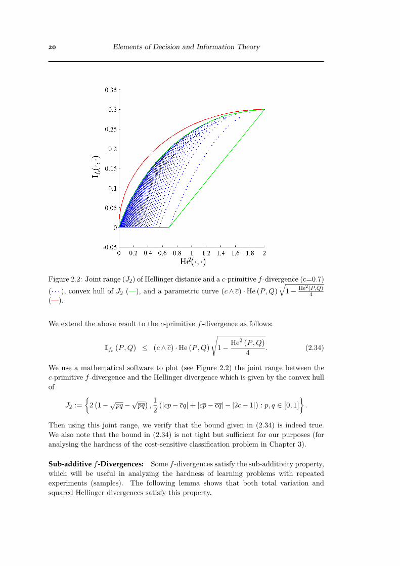
Figure 2.2: Joint range (J2) of Hellinger distance and a c-primitive f -divergence (c=0.7)(· · · ), convex hull of J2 (—), and a parametric curve
(
c · c)
· He(
P , Q)
Ò
1 ≠ He2(P ,Q)
4(—).
We extend the above result to the c-primitive f -divergence as follows:
Ifc (P , Q)
Æ(
c · c)
· He(
P , Q)
Û
1 ≠ He2(
P , Q)
4 . (2.34)
We use a mathematical software to plot (see Figure 2.2) the joint range between thec-primitive f -divergence and the Hellinger divergence which is given by the convex hullof
J2 :=;
2!
1 ≠ Ôpq ≠ Ô
pq"
, 12 (
|cp ≠ cq| + |cp ≠ cq| ≠ |2c ≠ 1|)
: p, q œ[
0, 1]
<
.
Then using this joint range, we verify that the bound given in (2.34) is indeed true.We also note that the bound in (2.34) is not tight but su�cient for our purposes (foranalysing the hardness of the cost-sensitive classification problem in Chapter 3).
Sub-additive f -Divergences: Some f -divergences satisfy the sub-additivity property,which will be useful in analyzing the hardness of learning problems with repeatedexperiments (samples). The following lemma shows that both total variation andsquared Hellinger divergences satisfy this property.

§2.4 Binary Experiments 21
Lemma 2.11. For all collections of distributions Pi, Qi œ P(
Oi), i œ [k]
dTV
A
kp
i=1Pi,
kp
i=1Qi
B
Æk
ÿ
i=1dTV (
Pi, Qi),
and
He2A
kp
i=1Pi,
kp
i=1Qi
B
Æk
ÿ
i=1He2
(
Pi, Qi).
Proof. Firstly(
P , Q)
‘æ dTV (
P , Q)
is a metric. Thus
dTV
A
kp
i=1Pi,
kp
i=1Qi
B
= dTV
A
P1 ¢A
kp
i=2Pi
B
, Q1 ¢A
kp
i=2Qi
BB
Æ dTV
A
P1 ¢A
kp
i=2Pi
B
, Q1 ¢A
kp
i=2Pi
BB
+ dTV
A
Q1 ¢A
kp
i=2Pi
B
, Q1 ¢A
kp
i=2Qi
BB
= dTV (
P1, Q1) + dTV
A
kp
i=2Pi,
kp
i=2Qi
B
,
where the second line follows by definition, the third follows from the triangle inequalityand the forth is easily verified from the definition of dTV (
·, ·)
. To complete the proofproceed inductively.
Let µ be a product measure on O1 ◊ O2, written as µ = µ1 ¢ µ2, where µi := µ ¶ fii
denotes the image measure of the projection fii : R2 –(
x1, x2) ‘æ fii (x1, x2) = xi w.r.t.µ. Also let P = P1 ¢ P2, and Q = Q1 ¢ Q2. Define p := dP
dµ , q := dQdµ , p1 := dP1
dµ1,
p2 := dP2dµ2
, q1 := dQ1dµ1
, and q2 := dQ2dµ2
. Then, by Tonelli’s theorem,
1 ≠ 12He2
(
P , Q)
=
⁄ Ôpqdµ
=
⁄ Ôp1q1dµ1 ·
⁄ Ôp2q2dµ2
=
3
1 ≠ 12He2
(
P1, Q1)
4
·3
1 ≠ 12He2
(
P2, Q2)
4
.
Thus we have
He2(
P , Q)
= 2 ≠ 23
1 ≠ 12He2
(
P1, Q1)
4
·3
1 ≠ 12He2
(
P2, Q2)
4
= He2(
P1, Q1) + He2(
P2, Q2) ≠ 12He2
(
P1, Q1)He2(
P2, Q2)
Æ He2(
P1, Q1) + He2(
P2, Q2) .
To complete the proof proceed the above process iteratively.

22 Elements of Decision and Information Theory
Chapter 3
Asymmetric Learning Problems
The central problem of this chapter is the cost-sensitive binary classification problem,where di�erent costs are associated with di�erent types of mistakes. Several importantmachine learning applications such as medical decision making, targeted marketing,and intrusion detection can be formalized as cost-sensitive classification setup (Abeet al. [2004]).
The chapter proceeds as follows. In section 3.1 we show that the abstract languageof transitions introduced in chapter 2, is general enough to capture many of the exist-ing practical problems in statistics and machine learning including the cost-sensitiveclassification problem. Then in section 3.2 we study the hardness of the cost-sensitiveclassification problem by extending the standard minimax lower bound of balancedbinary classification problem (due to Massart and Nédélec [2006]) to cost-sensitiveclassification problem.
In section 3.3 we study the hardness of the constrained learning problem (specif-ically constrained cost-sensitive classification), which naturally leads us to a detailedinvestigation of strong data processing inequalities. After reviewing the known resultsin strong data processing inequalities, we make some novel progress in the direction ofstrong data processing inequalities for binary symmetric channels. We also extend thewell-known contraction coe�cient theorem (Cohen et al. [1993]) for total variationaldivergence to c-primitive f -divergences.
Finally in section 3.4 we study the local privacy requirement as a form of constrainton learning problem. We review the decision theoretic reduction of the local privacyrequirement, and based on that we propose a prioritized (cost-sensitive) privacy defi-nition.
3.1 Preliminaries and Background
General Learning Task: Consider the General Learning Task represented by the fol-lowing transition diagram:
Q On AÁn A
(3.1)
23

24 Asymmetric Learning Problems
where Q, O, and A are parameter, observation, and action spaces respectively. Thetransitions Án and A denote repeated experiment of Á : Q O and algorithm respec-tively. Note that the repeated experiment Án induces the class of probability measuresgiven by PÁn (
On)
:= {Án (◊) := Á(
◊)
n : ◊ œ Q} (see Section 2.2.3). We recall the fol-lowing objects introduced in Chapter 2 :
Loss ¸ : Q ◊ A æ R
Regret D¸(
◊, a)
:= ¸(
◊, a)
≠ infaÕœA
¸(
◊, aÕ)
Full Risk R¸ (Án, ◊, A)
:= EOn
1 ≥Án(◊)
C
Ea≥A(On
1 )[
¸(
◊, a)]
D
RD¸ (Án, ◊, A)
:= EOn
1 ≥Án(◊)
C
Ea≥A(On
1 )[
D¸(
◊, a)]
D
Full Minimax Risk Rı¸ (Án) := inf
Asup◊œQ
R¸ (Án, ◊, A)
RıD¸ (Án) := inf
Asup◊œQ
RD¸ (Án, ◊, A)
.
One needs to carefully distinguish between the risk (and related notions) in terms ofloss and regret based on the subscript (see Remark 2.3). The general learning task iscompactly denoted by the tuple
(
¸, Án).In order to demonstrate the generality of the language of transitions, below we
discuss some specific instantiations (supervised learning, multi-class probability esti-mation, binary classification, and parameter estimation) of this general learning task.
Supervised Learning Problem: Let X ◊ Y be a measurable space, and let D be anunknown joint probability measure on X ◊ Y. The set X is called the instance space,the set Y the outcome space. Let S = {
(
Xi, Yi)}mi=1 œ
(
X ◊ Y)
m be a finite trainingsample, where each pair
(
Xi, Yi) is generated independently according to the unknownprobability measure D. Then the goal of a learning algorithm is to find a functionf : X æ Y which given a new instance x œ X , predicts its label to be ‚y = f
(
x)
.Here we rely on the fundamental assumption that both training and future (test)
data are generated by the same fixed underlying probability measure D, which, al-though unknown, allows us to infer from training data to future data and therefore togeneralize.
In order to measure the performance of a learning algorithm, we define an errorfunction d : Y ◊ Y æ R
+
, where d(
y, ‚y)
quantifies the discrepancy between the pre-dicted value ‚y and the actual value y. The performance of any function f : X æ Yis then measured in terms of its generalization error, which is defined as the expectederror:
erd (f , D)
:= E(X,Y)≥D
[
d(
Y, f(
X))]
, (3.2)
where the expectation is taken with respect to the probability measure D on the data(
X, Y)
. The best estimate fıD œ YX is therefore the one for which the generalization

§3.1 Preliminaries and Background 25
error is as small as possible, that is,
fıD := arg min
fœYXerd (f , D
)
. (3.3)
The function fıD is called the target hypothesis.
In order to avoid functions which over-fit the training sample and do not generalizewell on the test data, one usually imposes constraints on the function f . One way toimpose constraints is by restricting the possible choices of functions to a fixed classof functions from which the learning algorithm chooses its hypothesis. This functionclass is called the hypothesis class. Given a fixed hypothesis class F ™ YX , the goal ofa learning algorithm is thus to choose the hypothesis function fı in F which has thesmallest generalization error on data drawn according to the underlying probabilitymeasure D,
fıD,F := arg min
fœFerd (f , D
)
. (3.4)
We will assume in the following that such an fıD,F exists.
The supervised learning problem can be derived from the general learning task (3.1)with the following instantiation:
• the observation space is O = X ◊ Y, where X ™ Rd,
• the action space is A = F ™ YX ,
• the learning algorithm is A =
‚f , and
• the loss function is
¸d : Q ◊ F –(
◊, f)
‘æ ¸d (◊, f)
:= erd (f , Á(
◊))
œ R+
,
where Á(
◊)
is the probability measure associated with the parameter ◊ œ Q. Oneneeds to carefully distinguish between the error function d : Y ◊ Y æ R whichacts on the observation space, and the loss function ¸d : Q ◊ A æ R which actson the parameter and decision spaces.
Then the transition diagram for this supervised learning problem(
¸d, Án) is
Q(
X ◊ Y)
n FÁn‚f
. (3.5)
Binary Classification: When Y = {≠1, 1}, the supervised learning task (3.5) is calledbinary classification, which is a central problem in machine learning (Devroye et al.[2013]). A common error function for binary classification is simply the zero-one errordefined by d0≠1 (y, ‚y
)
= J‚y ”= yK. In this case the generalization error of a classifierf : X æ {≠1, 1} w.r.t. a probability measure D is simply the probability that itpredicts the wrong label on a randomly drawn example:
erd0≠1 (f , D)
:= E(X,Y)≥D
[
d0≠1 (Y, f(
X))]
= P(X,Y)≥D
[
f(
X)
”= Y]
.

26 Asymmetric Learning Problems
The optimal error over all possible classifiers f : X æ {≠1, 1} for a given probabilitymeasure D is called the Bayes error (minimum generalization error) associated withD:
erd0≠1 (D)
:= inffœ{≠1,1}X
erd0≠1 (f , D)
. (3.6)
It is easily verified that, if ÷D (
x)
is defined as the conditional probability (under D)of a positive label given x, ÷D (
x)
= PD [
Y = 1 | X = x]
, then the classifier fıD : X æ
{≠1, 1} given by
fıD (
x)
=
Y
]
[
1 if ÷D (
x)
Ø 1/2≠1 otherwise
achieves the Bayes error. Such a classifier is termed a Bayes classifier. In general, ÷D
is unknown so the above classifier cannot be constructed directly.
By defining ¸d0≠1 : Q ◊ F –(
◊, f)
‘æ ¸d0≠1 (◊, f)
:= erd0≠1 (f , Á(
◊))
œ R+
, thebinary classification problem
!
¸d0≠1 , Án"
can be represented by the following transitiondiagram:
Q(
X ◊ {≠1, 1})
n FÁn‚f
. (3.7)
Note that the repeated experiment Án above induces the class of probability measuresgiven by PÁn ((
X ◊ {≠1, 1})
n)
:= {Án (◊) := Á(
◊)
n œ P(
X ◊ {≠1, 1})
n : ◊ œ Q}. Us-ing the Bayes rule, the distribution PÁ(◊) can be decomposed as follows:
PÁ(◊) [X = x, Y = 1]
= PÁ(◊) [X = x]
· PÁ(◊) [Y = 1 | X = x]
= MÁ(◊) (x) · ÷Á(◊) (x) ,
where MÁ(◊) (x) := PÁ(◊) [X = x]
and ÷Á(◊) (x) := PÁ(◊) [Y = 1 | X = x]
. For simplicitywe will write PÁ(◊), MÁ(◊), ÷Á(◊), and fı
Á(◊) as P◊, M◊, ÷◊, and fı◊ respectively.
Cost-sensitive Binary Classification: Suppose we are given gene expression profilesfor some number of patients, together with labels for these patients indicating whetheror not they had a certain form of a disease. We want to design a learning algorithmwhich automatically recognizes the diseased patient based on the gene expression profileof a patient. In this case, there are di�erent costs associated with di�erent types ofmistakes (the health risk for a false label “no” is much higher than for a false “yes”),and the cost-sensitive error function (for c œ (0, 1)) can be used to capture this:
dc : Y ◊ Y –(
y, ‚y)
‘æ dc (y, ‚y)
:= J‚y ”= yK · {c · Jy = 1K+ c · Jy = ≠1K} ,
where c := 1 ≠ c. Then the performance measure (loss function) associated with theabove cost-sensitive error function is given by
¸dc : Q ◊ F –(
◊, f)
‘æ ¸dc (◊, f)
:= erdc (f , Á(
◊))
œ R+
,

§3.1 Preliminaries and Background 27
where
erdc (f , Á(
◊))
:= E(X,Y)≥Á(◊)
[
dc (Y, f(
X))]
= E(X,Y)≥Á(◊)
[
Jf(
X)
”= YK · {c · JY = 1K+ c · JY = ≠1K}]
.
For any ÷ : X æ[
0, 1]
, and f : X æ {≠1, 1}, define the conditional generalizationerror (given x œ X ) as
erdc (f , ÷; x)
:= EY≥÷(x)
[
dc (Y, f(
x))]
= c · ÷(
x)
· Jf(
x)
”= 1K+ c · ÷(
x)
· Jf(
x)
”= ≠1K,
where ÷(
x)
:= 1 ≠ ÷(
x)
. Then erdc (f , ÷; x)
is minimized by
fı(
x)
:= arg minfœ{≠1,1}X
EY≥÷(x)
[
dc (Y, f(
x))]
= sign1
c · ÷(
x)
≠ c · ÷(
x)
2
= sign(
÷(
x)
≠ c)
,
since erdc (fı, ÷; x
)
= c · ÷(
x)
· c · ÷(
x)
. In order to find the optimal classifier foreach ◊ œ Q (associated joint probability measure Á
(
◊)
on X ◊ {≠1, 1}) w.r.t. the cost-sensitive loss function, we note that
inffœ{≠1,1}X
¸dc (◊, f)
= inffœ{≠1,1}X
erdc (f , Á(
◊))
= inffœ{≠1,1}X
EX≥M◊
C
EY≥÷◊(X)
[
dc (Y, f(
X))]
D
= EX≥M◊
C
inffœ{≠1,1}X
EY≥÷◊(X)
[
dc (Y, f(
X))]
D
= ¸dc (◊, fı◊ ) ,
where M◊ (x) := PÁ(◊) [X = x]
, ÷◊ (x) := PÁ(◊) [Y = 1 | X = x]
, and fı◊ is given by
fı◊ (
x)
:=
Y
]
[
1, if ÷◊(x) Ø c
≠1, otherwise. (3.8)
We instantiate the following objects related to the cost-sensitive classification prob-lem
Regret D¸dc (◊, f)
:= ¸dc (◊, f)
≠ ¸dc (◊, fı◊ )
Full Risk RD¸dc
1
Án, ◊, ‚f2
:= E{(Xi,Yi)}n
i=1≥Án(◊)
S
U Ef≥‚f
(
{(Xi,Yi)}ni=1)
[
D¸dc (◊, f)]
T
V

28 Asymmetric Learning Problems
Full Minimax Risk RıD¸dc
(
Án) := inf‚f
sup◊œQ
RD¸dc
1
Án, ◊, ‚f2
.
The following lemma from Scott et al. [2012] will be used later.
Lemma 3.1 (Scott et al. [2012]). Consider the binary classification problem (3.7). Forany f œ F and c œ (0, 1),
D¸dc (◊, f)
=
12 · E
X≥M◊
[
|÷◊ (X) ≠ c| · |f(
X)
≠ fı◊ (
X)
|]
,
where fı◊ is given by (3.8).
Proof. Consider a fixed x œ X . Recall that
fı◊ (
x)
= arg minfœ{≠1,1}X
EY≥÷◊(x)
[
dc (Y, f(
x))]
= sign(
÷◊ (x) ≠ c)
.
Therefore inffœ{≠1,1}X EY≥÷◊(x)
[
dc (Y, f(
x))]
= EY≥÷◊(x)
[
dc (Y, fı◊ (
x))]
. This implies
EY≥÷◊(x)
[
dc (Y, f(
x))]
≠ EY≥÷◊(x)
[
dc (Y, fı◊ (
x))]
= c ÷◊ (x) Jf(x) ”= 1K+ c ÷◊ (x)Jf(x) ”= ≠1K
≠Ó
c ÷◊ (x) Jfı◊ (x) ”= 1K+ c ÷◊ (x)Jfı
◊ (x) ”= ≠1KÔ
= Jf(x) ”= fı◊ (x)K|÷◊ (x) ≠ c|
=
12 · |f(x) ≠ fı
◊ (x)| · |÷◊ (x) ≠ c|.
Then the proof is completed by noting that
¸dc (◊, f)
≠ ¸dc (◊, fı◊ ) = E
X≥M◊
C
EY≥÷◊(X)
[
dc (Y, f(
X))]
≠ EY≥÷◊(X)
[
dc (Y, fı◊ (
X))]
D
=
12 E
X≥M◊
[
|f(
X)
≠ fı◊ (
X)
| · |÷◊ (X) ≠ c|]
.
Parameter Estimation Problem: The main goal of a parameter problem is to ac-curately reconstruct the parameters of the original distribution from which the datais generated, using the loss function of the type fl : Q ◊ Q æ R. This problem isrepresented by the following transition diagram (with A = Q, and A =
‚◊):
Q On QÁn ‚◊
. (3.9)
Let ◊ : P(
O)
æ Q denote a function defined on P(
O)
, that is, a mappingP ‘æ ◊
(
P)
. The goal of the algorithm ‚◊ is to estimate the parameter ◊(
P)
based
§3.1 Preliminaries and Background 29
on observations On1 drawn from the (unknown) distribution P . In certain cases, the
parameter ◊(
P)
uniquely determines the underlying distribution; for example, in thecase of mean (◊) estimation problem from the normal distribution family P
(
O)
=
Ó
N(
◊, S)
: ◊ œ RdÔ
with known covariance matrix S, the parameter mapping ◊(
P)
=
EO≥P
[
O]
uniquely determines distributions in P(
O)
. In other scenarios, however, ◊
does not uniquely determine the distribution (confer Duchi [2016; accessed March 30,2017] for general treatment with this broader viewpoint of estimating functions of dis-tributions). In this chapter we consider the one-to-one function P ‘æ ◊
(
P)
.Observe that the class of probability measures induced by the repeated experiment
Án is written as PÁn (
On)
:= {Án (◊) := Á(
◊)
n œ P(
O)
n : ◊ œ Q}. Let fl : Q ◊ Q æ R
be a pseudo metric (that is, it satisfies symmetry and the triangle inequality) on Q.Then the minimax risk of this problem is defined as
Rıfl (Án) := inf
‚◊sup◊œQ
EOn
1 ≥Án(◊)
C
E◊≥‚◊(On
1 )
Ë
fl1
◊, ◊2È
D
. (3.10)
Hardness of a Problem via minimax lower bounds: Understanding the hardnessor fundamental limits of a learning problem is important for practice for the followingreasons:
• They give an estimate on the number of samples required for a good performanceof a learning algorithm.
• They give an intuition about the quantities and structural properties which areessential for a learning process and therefore about which problems are inherentlyeasier than others.
• They quantify the influence of parameters and indicate what prior knowledge isrelevant in a learning setting and therefore they guide the analysis, design, andimprovement of learning algorithms.
Note that the “hardness” here corresponds to lower bounds on sample complexity (andnot computational complexity). We demonstrate the hardness of a learning problem(3.1) (and the instantiations of it) by obtaining lower bounds for the minimax riskRı
¸ (Án) of it.In section 3.2 we review and extend techniques due to Le Cam [2012] and Assouad
[1983] for obtaining minimax lower bounds for learning problems. Both techniquesproceed by reducing the learning problem to an easier hypothesis testing problem[Tsybakov, 2009; Yang and Barron, 1999; Yu, 1997], then proving a lower bound onthe probability of error in testing problems.
Le Cam’s method, in its simplest form, provides lower bounds on the error in simplebinary hypothesis testing problems, by using the connection between hypothesis testingand total variation distance.
Consider the parameter estimation problem (3.9) with Q = {≠1, 1}m for some m,where the objective is to determine every bit of the underlying unknown parameter

30 Asymmetric Learning Problems
◊ œ {≠1, 1}m. In that setting, a key result known as Assouad’s lemma says that thedi�culty of estimating the entire bit string ◊ is related to the di�culty of estimatingeach bit of ◊ separately, assuming all other bits are already known.
3.2 Hardness of the Cost-sensitive Classification Problem
In this section we follow the presentation of Raginsky [2015; accessed March 30, 2017].Before studying the hardness of the cost-sensitive classification, we study the hardnessof the auxiliary problem of parameter estimation (3.9).
3.2.1 Minimax Lower Bounds for Parameter Estimation Problem
We derive the cost-dependent lower bound for Rıfl (Án) (defined in (3.10)) by extending
the standard Le Cam and Assouad’s techniques. We start with the two point methodintroduced by Lucien Le Cam for obtaining minimax lower bounds.
Proposition 3.2. For any c œ(
0, 1)
, the minimax risk Rıfl (Án) (given by (3.10)) of the
parameter estimation problem (3.9) with (pseudo metric) loss function fl : Q ◊ Q æ R
is bounded from below as follows:
Rıfl (Án) Ø sup
◊ ”=◊Õ
)
fl(
◊, ◊Õ)
·(
c · c ≠ Ifc (Án (◊) , Án (◊Õ)))
*
,
where fc is given by (2.27).
Proof. Let c œ(
0, 1)
be arbitrary but fixed. Consider any two fixed parameters ◊, ◊Õ œQ s.t. ◊ ”= ◊Õ and an arbitrary estimator ‚◊ : On Q. Let P n
◊ := Án (◊), andP n
◊Õ := Án (◊Õ)
(associated probability densities can be written as dP n◊ and dP n
◊Õ). Foran arbitrary (but fixed) set of observations on
1 œ On, when c · dP n◊Õ (on
1 ) Ø c · dP n◊ (
on1 ),
we have
c · dP n◊ (
on1 ) E
◊≥‚◊(on1 )
Ë
fl(◊, ◊)È
+ c · dP n◊Õ (on
1 ) E◊≥‚◊(on
1 )
Ë
fl(◊Õ, ◊)È
= c · dP n◊ (
on1 ) E
◊≥‚◊(on1 )
Ë
fl(◊, ◊) + fl(◊Õ, ◊)È
+
(
c · dP n◊Õ (on
1 ) ≠ c · dP n◊ (
on1 )) E
◊≥‚◊(on1 )
Ë
fl(◊Õ, ◊)È
(i)Ø c · dP n
◊ (
on1 ) E
◊≥‚◊(on1 )
Ë
fl(◊, ◊) + fl(◊Õ, ◊)È
(ii)Ø c · dP n
◊ (
on1 ) fl
(
◊, ◊Õ)
, (3.11)
where (i) is due to c · dP n◊Õ (on
1 ) Ø c · dP n◊ (
on1 ), and (ii) is due to the triangle inequality.
Similarly, for the case where c · dP n◊Õ (on
1 ) Æ c · dP n◊ (
on1 ), we get
c · dP n◊ (
on1 ) E
◊≥‚◊(on1 )
Ë
fl(◊, ◊)È
+ c · dP n◊Õ (on
1 ) E◊≥‚◊(on
1 )
Ë
fl(◊Õ, ◊)È
Ø c · dP n◊Õ (on
1 ) fl(
◊, ◊Õ)
.
(3.12)
§3.2 Hardness of the Cost-sensitive Classification Problem 31
By combining (3.11) and (3.12), and summing over all on1 œ On, we get, for any two
◊, ◊Õ œ Q and any estimator ‚◊,
c · EOn
1 ≥P n◊
C
E◊≥‚◊(On
1 )
Ë
fl(◊, ◊)È
D
+ c · EOn
1 ≥P n◊Õ
C
E◊≥‚◊(On
1 )
Ë
fl(◊Õ, ◊)È
D
(3.13)
Ø fl(
◊, ◊Õ)
·⁄
cdP n◊ · cdP n
◊Õ
= fl(
◊, ◊Õ)
·(
c · c ≠ Ifc (Pn◊ , P n
◊Õ)) , (3.14)
where the last equality follows from the definition of c-primitive f -divergences (2.30).By taking the supremum of both sides over the choices of ◊, ◊Õ (since then the two termsin (3.13) collapse to one), we have
sup◊œQ
EOn
1 ≥P n◊
C
E◊≥‚◊(On
1 )
Ë
fl(◊, ◊)È
D
Ø sup◊ ”=◊Õ
)
fl(
◊, ◊Õ)
·(
c · c ≠ Ifc (Án(◊), Án(◊Õ)
))
*
.
The proof is completed by taking the infimum of both sides over ‚◊.
By setting c =
12 in Proposition 3.2, we recover Le Cam’s (Le Cam [2012]) minimax
lower bound for parameter estimation problem (3.9):
Rıfl (Án) Ø 1
2 sup◊ ”=◊Õ
;
fl(
◊, ◊Õ)
·3
1 ≠ 12dTV (
Án (◊) , Án (◊Õ))
4<
,
since If 12(
P , Q)
=
14dTV (
P , Q)
(from (2.31) with c =
12). Now we provide an auxiliary
result which will be useful in deriving the cost-dependent minimax lower bounds viaAssouad’s lemma (Assouad [1983]).
Corollary 3.3. Let fi be any prior distribution on Q, and let µ be any joint probabilitydistribution of a random pair (◊, ◊Õ
) œ Q ◊ Q, such that the marginal distributions ofboth ◊ and ◊Õ are equal to fi. Then for any c œ
(
0, 1)
, the minimax risk Rıfl (Án) (given
by (3.10)) of the parameter estimation problem (3.9) is bounded from below as follows:
Rıfl (Án) Ø E
(◊,◊Õ)≥µ
[
fl(
◊, ◊Õ)
·(
c · c ≠ Ifc (Án (◊) , Án (◊Õ)))]
Proof. First observe that for any prior fi
Rıfl (Án) Ø inf
‚◊E
׳fi
C
EOn
1 ≥Án(◊)
C
E◊≥‚◊(On
1 )
Ë
fl(◊, ◊)È
DD
,
since the minimax risk can be lower bounded by the Bayesian risk (see Theorem 2.4).Then by taking expectation of both sides of (3.14) w.r.t µ and using the fact that,under µ, both ◊ and ◊Õ have the same distribution fi, the proof is completed.
Using the above corollary and extending the standard Assouad’s lemma, we derivethe cost-dependent minimax lower bound for the parameter estimation problem (3.9).

32 Asymmetric Learning Problems
Theorem 3.4. Let d œ N, Q = {≠1, 1}d and fl = flHa, where the Hamming distanceflHa is given by (2.1). Then for any c œ
(
0, 1)
, the minimax risk of the parameterestimation problem (3.9) satisfies
RıflHa (Án) Ø d
A
c · c ≠ max◊,◊Õ:flHa(◊,◊Õ
)=1Ifc (Án (◊) , Án (◊
Õ))
B
.
Proof. Recall that flHa(◊, ◊Õ) =
qdi=1 fli(◊, ◊Õ
), where fli(◊, ◊Õ) := J◊i ”= ◊Õ
iK, and each fli
is a pseudo metric. Let fi(◊) = 12d , ’◊ œ {≠1, 1}d. Also for each i œ
[
d]
, let µi be thedistribution in Q ◊ Q such that any random pair (◊, ◊Õ
) œ Q ◊ Q drawn according toµi satisfies
1. ◊ ≥ fi
2. fli(◊, ◊Õ) = 1, and flHa(◊, ◊Õ
) = 1 (◊ and ◊Õ di�er only in the i-th coordinate).
Then the marginal distribution of ◊Õ under µi isÿ
◊œ{≠1,1}d
µi(◊, ◊Õ) =
12d
ÿ
◊œ{≠1,1}d
J◊i ”= ◊Õi and ◊j = ◊Õ
j , j ”= iK = 12d
= fi(◊Õ),
since by construction of µ, flHa (◊, ◊Õ)
= 1 and for each ◊Õ there is only one ◊ that di�ersfrom it in a single coordinate. Now consider
RıflHa (Án)
(i)Ø inf
‚◊E
׳fi
C
EOn
1 ≥Án(◊)
C
E◊≥‚◊(On
1 )
Ë
flHa1
◊, ◊2È
DD
(ii)= inf
‚◊
dÿ
i=1E
׳fi
C
EOn
1 ≥Án(◊)
C
E◊≥‚◊(On
1 )
Ë
fli
1
◊, ◊2È
DD
Ød
ÿ
i=1inf‚◊
E׳fi
C
EOn
1 ≥Án(◊)
C
E◊≥‚◊(On
1 )
Ë
fli
1
◊, ◊2È
DD
(iii)Ø
dÿ
i=1E
(◊,◊Õ)≥µi
[
fli (◊, ◊Õ)
·(
c · c ≠ Ifc (Án (◊) , Án (◊Õ)))]
(iv)=
dÿ
i=1E
(◊,◊Õ)≥µi
[(
c · c ≠ Ifc (Án (◊) , Án (◊Õ)))]
Ød
ÿ
i=1min
◊,◊Õ:flHa(◊,◊Õ)=1
(
c · c ≠ Ifc (Án (◊) , Án (◊Õ)))
= d
A
c · c ≠ max◊,◊Õ:flHa(◊,◊Õ
)=1Ifc (Án (◊) , Án (◊
Õ))
B
,
where (i) is due to the fact that the minimax risk is lower bounded by the Bayesian risk(see Theorem 2.4), (ii) is due to flHa(◊, ◊Õ
) =
qdi=1 fli(◊, ◊Õ
), (iii) is by Corollary 3.3,and (iv) is by the fact that fli(◊, ◊Õ
) = 1 under µi for every i.

§3.2 Hardness of the Cost-sensitive Classification Problem 33
If we re-normalize Ifc (·, ·)
by c · c, and define Iúfc(
·, ·)
:= 1c·cIfc (·, ·
)
, then theminimax lower bound in Theorem 3.4 can be written as follows:
RıflHa (Án) Ø d ·
(
c · c)
C
1 ≠ max◊,◊Õ:flHa(◊,◊Õ
)=1Iú
fc(
Án (◊) , Án (◊Õ))
D
.
Also note that, by setting c =
12 in Theorem 3.4, we recover the standard Assouad’s
lemma (Assouad [1983]):
RıflHa (Án) Ø d
2
A
1 ≠ 12 max
◊,◊Õ:flHa(◊,◊Õ)=1
dTV (
Án (◊) , Án (◊Õ))
B
.
We use the following two properties of the Hellinger distance He2(
P , Q)
(shown inChapter 2) to derive a more practically useful version of Assouad’s lemma:
• Ifc (P , Q)
Æ(
c · c)
· He(
P , Q)
, for all distributions P , Q œ P(
O)
(refer (2.34))
• He21
oki=1 Pi,
oki=1 Qi
2
Æ qki=1 He2
(
Pi, Qi), for all distributions Pi, Qi œP(
Oi), i œ [k]
Armed with these facts, we prove the following version of Assouad’s lemma:
Corollary 3.5. Let O be some set and c œ [0, 1]. Define
PÁ (O)
:=Ó
Á(
◊)
œ P(
O)
: ◊ œ {≠1, 1}dÔ
be a class of probability measures induced by the transition Á : {≠1, 1}d O. Supposethat there exists some function – :
[
0, 1]
æ R+
, such that
He2(
Á(
◊)
, Á(
◊Õ))
Æ –(
c)
, if flHa (◊, ◊Õ)
= 1,
i.e. the two probability distributions Á(
◊)
and Á(
◊Õ)
(associated with the two parameters◊ and ◊Õ which di�er only in one coordinate) are su�ciently close w.r.t. Hellinger dis-tance. Then the minimax risk of the parameter estimation problem (3.9) with parameterspace Q = {≠1, 1}d and the loss function fl = flHa is bounded below by
RıflHa (Án) Ø d · (c · c) ·
3
1 ≠Ò
–(
c)
n4
. (3.15)
Proof. For any two ◊, ◊Õ œ Q with flHa (◊, ◊Õ)
= 1, we have
Ifc (Án (◊) , Án (◊Õ))
Æ(
c · c)
· He(
Án (◊) , Án (◊Õ))
Æ(
c · c)
·ˆ
ı
ı
Ù
nÿ
i=1He2
(
Á(
◊)
, Á(
◊Õ))
Æ(
c · c)
·Ò
–(
c)
n

34 Asymmetric Learning Problems
Substituting this bound into Theorem 3.4 completes the proof.
The number of training samples n appear in the minimax lower bound (3.15). Thusthe hardness of the problem can be expressed as a function of the sample size alongwith other problem specific parameters.
3.2.2 Minimax Lower Bounds for Cost-sensitive Classification Problem
A natural question to ask regarding cost-sensitive classification problem is how does thehardness of the problem depend upon the cost parameter c œ
[
0, 1]
. Let F ™ {≠1, 1}X
be the action space and h œ[
0, c · c]
be the margin parameter whose interpretationis explained below. Then we choose a parameter space Qh,F (thus the experimentÁh,F : Qh,F (
X ◊ {≠1, 1})
) such that:
1. ’◊ œ Qh,F , fı◊ œ F , where fı
◊ is given by (3.8). That is we restrict the parameterspace s.t. the Bayes classifier associated with each choice of parameter lies withinthe predetermined function class F .
2.|÷◊ (X) ≠ c| Ø h a.s. ’◊ œ Qh,F . (3.16)
This condition is a generalized notion of Massart noise condition with margin h œ[
0, c · c]
(Massart and Nédélec [2006]). The motivation for this condition is wellestablished by Massart and Nédélec [2006]. They have argued that under certain“margin” type conditions ([Vapnik and Chervonenkis, 1974; Tsybakov, 2004])like this, it is possible to design learning algorithms for the binary classificationproblem, with better rates compared to the case where no such condition issatisfied.
Thus we consider the problem represented by following transition diagram
Qh,F (
X ◊ {≠1, 1})
n FÁn‚f
, (3.17)
and the minimax risk (in terms of regret) of it given by
RıD¸dc
(
Án) := inf‚f
sup◊œQh,F
E{(Xi,Yi)}n
i=1≥Án(◊)
S
U Ef≥‚f
(
{(Xi,Yi)}ni=1)
[
D¸dc (◊, f)]
T
V. (3.18)
The following is a generalization of the result proved in [Massart and Nédélec, 2006,Theorem 4] for c =
12 .
Theorem 3.6. Let F be a VC class of binary-valued functions on X with VC dimension(refer section 3.6.1) V Ø 2. Then for any n Ø V and any h œ [0, c · c], the minimaxrisk (3.18) of the cost-sensitive binary classification problem (3.17) is lower bounded as

§3.2 Hardness of the Cost-sensitive Classification Problem 35
follows:
RıD¸dc
(
Án) Ø K · (c · c) · min
Q
a
Û
(c · c)V
n, (c · c) · V
nh
R
b
where K > 0 is some absolute constant.
Proof. Instantiate Q = A = B := {≠1, 1}V ≠1, O = X ◊ {≠1, 1}, and A =
‚b in thegeneral learning task (3.1). Then the resulting parameter estimation problem can berepresented by the following transition diagram:
B On BÁn ‚b
.
Let PÁn (
On)
:= {Án (b) := Á(
b)
n œ P(
O)
n : b œ B} be the class of probability mea-sures induced by the experiment Án. Then the minimax risk of this problem w.r.t.Hamming distance flHa is given by
RıflHa (Án) = inf
‚bmaxbœB
EOn
1 ≥Án(b)
C
EbÕ≥‚b(On
1 )[
flHa (b, bÕ)]
D
.
Observe that PÁ(b) [X = x, Y = y]
= PÁ(b) [X = x]
· PÁ(b) [Y = y|X = x]
for b œ B(by Bayes rule). For simplicity, we will write PÁ(b) [·] as Pb [·]. Now we will constructthese distributions.
Construction of marginal distribution Pb [X = x]
, x œ X : Since F is a VCclass with VC dimension V , ÷ {x1, ..., xV } µ X that is shattered, i.e. for any — œ{≠1, 1}V , ÷f œ F s.t. f(xi) = —i, ’i œ
[
V]
. Given p œ[
0, 1/(V ≠ 1)]
, for each b œ B,let
Pb [X = x]
=
Y
_
_
]
_
_
[
p, if x = xi for some i œ[
V ≠ 1]
1 ≠ (V ≠ 1)p, if x = xV
0, otherwise(3.19)
A particular value for p will be chosen later.Construction of conditional distribution Pb [Y = y|X = x
]
, y œ {≠1, 1} , x œX : For each b œ B, let
÷b (x) := Pb [Y = 1|X = x]
=
Y
_
_
]
_
_
[
c ≠ h, if x = xi for some i œ[
V ≠ 1]
, and bi = ≠1c + h, if x = xi for some i œ
[
V ≠ 1]
, and bi = 10, otherwise.
(3.20)Then the corresponding Bayes classifier can be given as follows:
fıb (x) =
Y
_
_
]
_
_
[
≠1, if x = xi for some i œ[
V ≠ 1]
, and bi = ≠11, if x = xi for some i œ
[
V ≠ 1]
, and bi = 1≠1, otherwise
(3.21)

36 Asymmetric Learning Problems
Now we show that {Á(
b)
: b œ B} ™ {Á(
◊)
: ◊ œ Qh,F}. First of all, from (3.20) we seethat |÷b (x) ≠ c| Ø h for all x (indeed, |÷b (x) ≠ c| = h when x œ {x1, ..., xV ≠1}, and|÷b (x)≠ c| = c otherwise). Second, because {x1, ..., xV } is shattered by F , there existsat least one f œ F , such that fı
b (x) = f(x) for all x œ {x1, ..., xV }. Thus, we getB µ Qh,F .
Reduction to Parameter Estimation Problem: We start with the followingobservation
RıD¸dc
(
Án) Ø inf‚f
maxbœB
E{(Xi,Yi)}n
i=1≥Án(b)
S
U Ef≥‚f
(
{(Xi,Yi)}ni=1)
[
¸dc (b, f)
≠ ¸dc (b, fıb )]
T
V,
since B µ Qh,F . Define M◊ (x) := P◊ [X = x]
, and ÷◊ (x) := P◊ [Y = 1 | X = x]
, forx œ X . By Lemma 3.1, for any classifier f : X æ {≠1, 1} and any ◊ œ Qh,F , we have
¸dc (◊, f)
≠ ¸dc (◊, fı◊ ) =
12 · E
X≥M◊
[
|÷◊ (X) ≠ c| · |f(
X)
≠ fı◊ (
X)
|]
.
If ◊ œ Qh,F , then using the above equation and the margin condition (3.16) we get
¸dc (◊, f)
≠ ¸dc (◊, fı◊ ) Ø h
2 · EX≥M◊
[
|f(
X)
≠ fı◊ (
X)
|]
=
h
2 · Îf ≠ fı◊ ÎL1(M◊)
,
where ÎfÎL1(M◊)is given by (2.5) with p = 1 and µ = M◊. Since there is no confusion,
we can simply drop M◊ and write the L1 norm as ηÎL1. Hence we have
inf‚f
maxbœB
E{(Xi,Yi)}n
i=1≥Án(b)
S
U Ef≥‚f
(
{(Xi,Yi)}ni=1)
[
¸dc (b, f)
≠ ¸dc (b, fıb )]
T
V
Ø h
2 · inf‚f
maxbœB
E{(Xi,Yi)}n
i=1≥Án(b)
S
U Ef≥‚f
(
{(Xi,Yi)}ni=1)
Ë
Îf ≠ fıb ÎL1
È
T
V.
Definebf := arg min
bœBÎf ≠ fı
b ÎL1.
Then for any b œ B,.
.
.
fıbf
≠ fıb
.
.
.
L1Æ
.
.
.
fıbf
≠ f.
.
.
L1+ Îf ≠ fı
b ÎL1Æ 2 Îf ≠ fı
b ÎL1,
where the first inequality is due to the triangle inequality and the second follows fromthe definitions of bf and fı
◊ . Thus we have
inf‚f
maxbœB
E{(Xi,Yi)}n
i=1≥Án(b)
S
U Ef≥‚f
(
{(Xi,Yi)}ni=1)
[
¸dc (b, f)
≠ ¸dc (b, fıb )]
T
V
Ø h
4 · inf‚f
maxbœB
E{(Xi,Yi)}n
i=1≥Án(b)
S
U Ef≥‚f
(
{(Xi,Yi)}ni=1)
5
.
.
.
fıbf
≠ fıb
.
.
.
L1
6
T
V

§3.2 Hardness of the Cost-sensitive Classification Problem 37
=
h
4 · inf‚b
maxbœB
E{(Xi,Yi)}n
i=1≥Án(b)
S
U EbÕ≥‚b
(
{(Xi,Yi)}ni=1)
Ë
ÎfıbÕ ≠ fı
b ÎL1
È
T
V.
For any two b, bÕ œ B, we have
ÎfıbÕ ≠ fı
b ÎL1=
⁄
X|fı
bÕ(x) ≠ fıb (x)|Pb [X = x
]
dx
= pV ≠1ÿ
i=1|fı
bÕ(xi) ≠ fıb (xi)|
= pV ≠1ÿ
i=1|bÕ
i ≠ bi|
= 2p · flHa (b, bÕ)
,
where the second and third equalities are from (3.19) and (3.21). Finally we get
inf‚f
maxbœB
E{(Xi,Yi)}n
i=1≥Án(b)
S
U Ef≥‚f
(
{(Xi,Yi)}ni=1)
[
¸dc (b, f)
≠ ¸dc (b, fıb )]
T
V
Ø ph
2 · inf‚b
maxbœB
E{(Xi,Yi)}n
i=1≥Án(b)
S
U EbÕ≥‚b
(
{(Xi,Yi)}ni=1)
[
flHa (b, bÕ)]
T
V
=
ph
2 · RıflHa (Án) . (3.22)
Applying Assouad’s Lemma: For any two b, bÕ œ B we have
He2(
Á(
b)
, Á(
bÕ))
=
Vÿ
i=1
ÿ
yœ{≠1,1}
3
Ò
Pb [X = xi, Y = y]
≠Ò
PbÕ[
X = xi, Y = y]
42
= pV ≠1ÿ
i=1
ÿ
yœ{≠1,1}
3
Ò
Pb [Y = y|X = xi] ≠Ò
PbÕ[
Y = y|X = xi]
42
= pV ≠1ÿ
i=1Jbi ”= bÕ
iKI
1Ôc ≠ h ≠ Ô
c + h22
+
3
Ò
c ≠ h ≠Ò
c + h42
J
= 2p1
1 ≠
c2 ≠ h2 ≠
c2 ≠ h22
flHa (b, bÕ)
,
where the second and third equalities are from (3.19) and (3.20). Thus the conditionof the Corollary 3.5 is satisfied with
2p1
1 ≠
c2 ≠ h2 ≠
c2 ≠ h22
Æ 4ph2
c · c=: –
(
c)
,

38 Asymmetric Learning Problems
where the inequality is from Lemma 3.7 (see below). Therefore we get
inf‚f
maxbœB
E{(Xi,Yi)}n
i=1≥Án(b)
S
U Ef≥‚f
(
{(Xi,Yi)}ni=1)
[
¸dc (b, f)
≠ ¸dc (b, fıb )]
T
V
Ø ph(V ≠ 1)2
Q
ac · c ≠ c · c ·Û
4ph2
c · cn
R
b
=
ph(V ≠ 1)2
!
c · c ≠ 2hÔ
c · c · pn"
,
where the first inequality is due to (3.15) and (3.22). If we let p =
c·c9nh2 , then the term
in the parentheses will be equal to c·c3 , and
inf‚f
maxbœB
E{(Xi,Yi)}n
i=1≥Án(b)
S
U Ef≥‚f
(
{(Xi,Yi)}ni=1)
[
¸dc (b, f)
≠ ¸dc (b, fıb )]
T
V Ø (c · c)2(V ≠ 1)
54nh,
assuming that the condition p Æ 1/(V ≠ 1) holds. This will be the case if h ØÒ
c·c(V ≠1)9n . Therefore
RıD¸dc
(
Án) Ø (c · c)2(V ≠ 1)
54nh, if h Ø
Û
c · c(V ≠ 1)9n
. (3.23)
If h ÆÒ
c·c(V ≠1)9n , we can use the above construction with h =
Ò
c·c(V ≠1)9n . Then,
because Qh,F ™ Qh,F whenever h Ø h, we see that
inf‚f
sup◊œQh,F
E{(Xi,Yi)}n
i=1≥Án(◊)
S
U Ef≥‚f
(
{(Xi,Yi)}ni=1)
[
¸dc (◊, f)
≠ ¸dc (◊, fı◊ )]
T
V
Ø inf‚f
sup◊œQh,F
E{(Xi,Yi)}n
i=1≥Án(◊)
S
U Ef≥‚f
(
{(Xi,Yi)}ni=1)
[
¸dc (◊, f)
≠ ¸dc (◊, fı◊ )]
T
V
Ø (c · c)2(V ≠ 1)
54nh
=
(c · c)32
18
Û
V ≠ 1n
, if h ÆÛ
c · c(V ≠ 1)9n
. (3.24)
Observe that (c·c)2(V ≠1)
54nh Æ (c·c)32
18
Ò
V ≠1n if h Ø
Ò
c·c(V ≠1)9n , and (c·c)2
(V ≠1)54nh > (c·c)
32
18
Ò
V ≠1n
otherwise. Then combining (3.23) and (3.24) completes the proof.
Lemma 3.7. For h œ[
0, c · c]
, we have 1 ≠ Ôc2 ≠ h2 ≠ Ô
c2 ≠ h2 Æ 2 h2
c·c .
Proof. Let A = 1 ≠ Ôc2 ≠ h2 ≠ Ô
c2 ≠ h2. Take series expansion of A w.r.t. h to get
A =
12
31c+
1c
4
h2+
18
3 1c3 +
1c3
4
h4+
116
3 1c5 +
1c5
4
h6+
5128
3 1c7 +
1c7
4
h8

§3.2 Hardness of the Cost-sensitive Classification Problem 39
+
7256
3 1c9 +
1c9
4
h10+
211024
3 1c11 +
1c11
4
h12+
332048
3 1c13 +
1c13
4
h14+ · · · .
Now 12
1
1c +
1c
2
Æ 1c ‚ 1
c =
1c·c (since average is less than maximum). Thus
A Æ h
C
h
c · c+
14
h3
(
c · c)
3 +
18
h5
(
c · c)
5 +
564
h7
(
c · c)
7 +
7128
h9
(
c · c)
9 +
21512
h11
(
c · c)
11 + · · ·D
.
Now we have
h Æ c · c =∆ h
c · cÆ 1
=∆3
h
c · c
4–
Æ h
c · c, ’– Ø 1.
Thus
A Æh5
h
c · c+
h
c · c
;14 +
18 +
564 +
7128 +
21512 + · · ·
<6
Æh5 2h
c · c
6
=
2h2
c · c,
where the second inequality follows from the fact that (can be shown with the aid ofcomputer or using the properties of gamma function)
14 +
18 +
564 +
7128 +
21512 + · · · Æ 1.
When h = 0 (or being too small), we get a minimax lower bound of order(
c · c)
32 ·
Ò
Vn , and when h = c · c, we obtain a bound of the order
(
c · c)
· Vn .
When c = 1/2 in Theorem 3.6, we recover the standard minimax lower bounds forbalanced binary classification (with zero-one loss function) presented in [Massart andNédélec, 2006, Theorem 4]:
RıD¸0≠1 (Án) Ø K Õ · min
Q
a
Û
V
n, V
nh
R
b ,
for some constant K Õ > 0.It would be interesting to study the hardness of the following classification problem
settings which are closely related to the binary cost-sensitive classification problem thatwe considered in this thesis:
1. Cost-sensitive classification with example dependent costs ([Zadrozny and Elkan,2001; Zadrozny et al., 2003]).
2. Binary classification problem w.r.t. generalized performance measures (Koyejoet al. [2014]) such as arithmetic, geometric and harmonic means of the true posi-
40 Asymmetric Learning Problems
tive and true negative rates. These measures are more appropriate for imbalancedclassification problem ([Cardie and Nowe, 1997; Elkan, 2001]) than the usual clas-sification accuracy.
3.3 Constrained Learning Problem
In the normal theoretical analysis of the learning problem (3.1), it is assumed that thedecision maker has access to clean data (in On), that their observations are from thepattern they are expected to predict. In the real world, this is usually not the case,data is normally corrupted or needs to be corrupted to meet privacy requirements. Wecan formalize these constraints (noisy data and privacy requirements) in the languageof transitions by introducing the channel T : O ‚O, where ‚O is the new observationspace for the decision maker. The Constrained learning task (denoted by
(
¸, Án, T1:n),where Án is the repeated experiment (2.16), and T1:n is the parallelized transition(2.18)), can be represented by the following transition diagram:
Q On‚On AÁn T1:n A
Án :=(
T ¶ Á)n . (3.25)
For convenience we define the corrupted experiment Á := T ¶ Á, and denote the re-peated corrupted experiment by Án. We study the hardness of this constrained learningproblem (3.25) by producing the minimax lower bounds of it. From the Weak DataProcessing Inequality (If (Án) Æ If (Án)), we have
Rı¸ (Án) Ø Rı
¸ (Án) ,
i.e. the constrained problem is harder than the original unconstrained problem. Thenthe minimax lower bounds for the unconstrained problem (3.1) are applicable to thisconstrained task as well. However, this provides us with no means to compare variouschoices of channel T for a given problem.
For some T , the weak data processing theorem can be strengthened, in the sensethat one can find a constant called the contraction coe�cient ÷f (T )
< 1 (formallydefined in Definition 3.8) such that If (Án) Æ ÷f (T )
If (Án), for all experiments Á : Q O. The strengthened inequality is called the Strong Data Processing Inequality. Thecontraction coe�cient ÷f (T )
provides a means to measure the amount of corruptionpresent in T . For example if T is constant and maps all input distributions to the sameoutput distribution, then ÷f (T )
= 0. If T is an invertible function, then ÷f (T )
= 1.Together with the minimax lower bounds of unconstrained problem, this strong dataprocessing inequality leads to meaningful lower bounds that allow the comparison ofdi�erent corrupted experiments. In what follows we will present some new results onstrong data processing inequalities. Specifically, we will derive an explicit closed form

§3.3 Constrained Learning Problem 41
for the contraction coe�cient of any channel w.r.t. c-primitive f -divergence, and obtaine�ciently computable lower bounds for the contraction coe�cients of binary symmetricchannels w.r.t. symmetric f -divergences.
3.3.1 Strong Data Processing Inequalities
Consider a channel T : X Y, with finite input (X ) and output (Y) spaces (alsolet |X | Ø 2 and |Y| Ø 2). Observe that T can also be viewed as an experiment witha di�erent parameter space X . The classes of probability measures generated by theexperiment Á and the channel T are given by PÁ (O)
:= {Á(
◊)
œ P(
O)
: ◊ œ Q} andPT (
Y)
:= {T(
x)
œ P(
Y)
: x œ X } respectively.Strong data processing inequalities has become an intensive research area in the
information theory community recently (see Raginsky [2014] and references therein).Early work includes Ahlswede and Gács [1976] and Dobrushin [1956a] (see Cohen et al.[1993] for further history).
Below we formally define the contraction coe�cient ÷f (T )
of the channel T w.r.t.f -divergence. Recall that Pú (X )
means the set of all strictly positive distributionsover X .
Definition 3.8. Given a transition T : X Y and µ œ Pú (X )
, we define
÷f (µ, T ) := sup‹ ”=µ,‹œP(X )
If (T ¶ ‹, T ¶ µ)
If (‹, µ)
÷f (T ) := supµœPú(X )
÷f (µ, T ).
If ÷f (µ, T ) < 1, we say that T satisfies the strong data processing inequality (SDPI) atµ w.r.t. f-divergence i.e.
If (T ¶ ‹, T ¶ µ)
Æ ÷f (µ, T )If (‹, µ)
for all ‹ œ P(
X)
. Moreover if ÷f (T ) < 1 we say that T satisfies the SDPI w.r.t.f-divergence i.e.
If (T ¶ ‹, T ¶ µ)
Æ ÷f (T )If (‹, µ)
for all ‹ œ P(
X)
and µ œ Pú (X )
.
Cohen et al. [1993] showed that the contraction coe�cient ÷f (T ) of any channelT with respect to any f -divergence is universally upper-bounded by the so-called Do-brushin’s coe�cient of T [Dobrushin, 1956a,b]. Dobrushin’s coe�cient is extensivelystudied in the context of Markov chains (see Paz [1971] and Isaacson and Madsen [1976]for detailed discussions).
Theorem 3.9. Define the Dobrushin’s coe�cient [Dobrushin, 1956a,b] of a channelT œ M
(
X , Y)
asË(
T)
:=12 max
x,xÕœXdTV (
T(
x)
, T(
xÕ))
. (3.26)

42 Asymmetric Learning Problems
Then the contraction coe�cient of the channel T w.r.t. any f-divergence is boundedabove as follows
÷f (T )
Æ ÷TV (
T)
= Ë(
T)
, (3.27)
where ÷TV (
T)
is the contraction coe�cient of the channel T w.r.t. total variationdivergence (i.e. TV
(
x)
= |x ≠ 1|).We are interested in the question of how loose the bound in Theorem 3.9 can be. For
this we study the contraction coe�cients w.r.t. c-primitive f -divergences (2.32). Recallthat any f -divergence can be written as a weighted integral of c-primitive f -divergencesas given in Theorem 2.7.
As a starting point, we define the generalized Dobrushin’s coe�cient of a channelT : X Y as follows
Ëc(T ) :=1
c · c· max
x,xÕœXIfc (T (x), T (xÕ
)
)
, (3.28)
where c œ(
0, 1)
and Ë0(T ) = Ë1(T ) := 0. Note that when c =
12 , this gives the
standard Dobrushin’s coe�cient. From the definition (3.28) we can note the followingproperties of Ëc(T ):
1. For a given T , Ëc(T ) is symmetric in c about 12 i.e. Ëc = Ëc.
2. For the fully-informative channel we have Ëc(Tid) = 1 (can be easily shown fromthe definition), and for the non-informative channel Ëc(T•X ) = 0. Thus for anychannel T we have 0 Æ Ëc(T ) Æ 1.
3. For two channels T1 and T2, it is possible that Ëc(T1) > Ëc(T2) and ËcÕ(T1) <
ËcÕ(T2) i.e. optimal channel choice based on contraction coe�cient will depend
on c (see Figure 3.1).
We have plotted the generalized Dobrushin’s coe�cient for binary channels T :[
2]
[
2]
, and ternary channels T :[
3]
[
3]
. Based on those observations (seeFigure 3.1), we conjecture the following properties of Ëc(T ):
1. For a given T , and for any 0 < c < cÕ < 0.5, Ëc(T ) Æ ËcÕ(T ).
2. The maximum point of the curve Ëc(T ) always occurs at c =
12 (this matches
the fact that ÷TV(T ) upper bounds the contraction coe�cient ÷f (T ) of any f -divergence).
We now relate the contraction coe�cient ÷fc(T ) w.r.t. c-primitive f -divergence tothe generalized Dobrushin’s coe�cient Ëc(T ) defined above.
Theorem 3.10. For any T œ M(
X , Y)
, and c œ[
0, 1]
we have
÷fc (T )
= Ëc (T )
where ÷fc (T )
is the contraction coe�cient of the channel T w.r.t. c-primitive f-divergence.

§3.3 Constrained Learning Problem 43
1
1
T = T•X
T = Tid
T = T1
T = T2c
Ëc(T )
Figure 3.1: Generalized Dobrushin’s coe�cient of two arbitrary channels T1 =
C
0.8 0.20.2 0.8
D
(—) and T2 =
C
0.1 0.60.9 0.4
D
(—), fully-informative channel Tid (—), and
non-informative channel T•X (—).
Proof. We follow the proof of Theorem 3.1 in [Raginsky, 2014].We start with the following generalization of strong Markov contraction lemma from
Cohen et al. [1993]: for any signed measure ‹ on X , any c œ[
0, 1]
and any Markovkernel T œ M
(
X , Y)
, we have
ÎT ¶ ‹ÎTV Æ Ëc (T )
΋ÎTV +
(
1 ≠ Ëc (T ))
|‹(
X)
|, (3.29)
where the total variation norm ΋ÎTV of signed measure ‹ is given by ΋ÎTV :=q
xœX |‹(
x)
|. This can be shown by simply following through the steps of the proofof Lemma 3.2 in Cohen et al. [1993]. Let ‹ = c‹ ≠ cµ, where ‹ and µ are probabilitymeasures on X . Then T ¶ ‹ = cT ¶ ‹ ≠ cT ¶ µ and |‹
(
X)
| = |2c ≠ 1|. By using (3.29)and the definition of c-primitive f -divergence (2.32), we get
dTV (
cT ¶ ‹, cT ¶ µ)
Æ Ëc (T )
dTV (
c‹, cµ)
+
(
1 ≠ Ëc (T ))
|2c ≠ 1|=∆ dTV (
cT ¶ ‹, cT ¶ µ)
≠ |2c ≠ 1| Æ Ëc (T )
{dTV (
c‹, cµ)
≠ |2c ≠ 1|}=∆ Ifc (T ¶ ‹, T ¶ µ
)
Æ Ëc (T )
· Ifc (‹, µ)
.
Now it remains to show that this bound is achieved for some probability measures µand ‹.
To that end, let us first assume that |X | > 2. Let x0, x1 œ X achieve the maximumin (3.28), pick some ‘1, ‘2, ‘ œ (0, 1) such that ‘1 ”= ‘2, ‘1 + ‘ < 1, ‘2 + ‘ < 1, andconsider the following probability distributions:
• ‹ that puts the mass 1 ≠ ‘1 ≠ ‘ on x0, ‘1 on x1, and distributes the remainingmass of ‘ evenly among the set X \ {x0, x1};
• µ that puts the mass 1 ≠ ‘2 ≠ ‘ on x0, ‘2 on x1, and distributes the remaining

44 Asymmetric Learning Problems
mass of ‘ evenly among the set X \ {x0, x1}.
Then a simple calculation (using a mathematical software) gives
Ifc (‹, µ)
=
12
Ó
|c‘1 ≠ c‘2| + |c(
‘1 + ‘)
≠ c(
‘2 + ‘)
| +(
|X | ≠ 2)
· |c‘ ≠ c‘| ≠ |2c ≠ 1|Ô
Ifc (T ¶ ‹, T ¶ µ)
=Ëc (T )
· Ifc (‹, µ)
.
For |X | = 2, the idea is the same, except that there is no need for the extra slack ‘.
From the above theorem, for any T œ M(
X , Y)
and for all P , Q œ P(
X)
, we have
Ifc (T ¶ P , T ¶ Q)
Æ Ëc (T )
Ifc (P , Q)
.
Thus for any general f -divergence (using the weighted integral representation) we get
If (T ¶ P , T ¶ Q)
=
⁄ 1
0“f (c) Ifc (T ¶ P , T ¶ Q
)
dc
Æ⁄ 1
0Ëc (T )
“f (c) Ifc (P , Q)
dc (3.30)
Æ Ë 12(
T)
· If (P , Q)
,
where the last inequality is due to the fact that Ëc (T )
Æ Ë 12(
T)
. Even though thisdoesn’t fully answer the question of how loose the universal bound (3.27) can be, (3.30)along with the Figure 3.1, sheds some light in that direction.
Remark 3.11. Let f be a convex function with f(
1)
= 0, which can be written in thefollowing form
f(u) = –u + —u2+
⁄ Œ
0
3
tu
1 + t2 ≠ u
u + t
4
v(dt),
where – œ R, — Ø 0, and v is a non-negative measure on R+
such thats Œ
01
1+t2 v(dt) <Œ. Note that for such function f , we have
f ÕÕ(u) = 2— + 2
⁄ Œ
0
t
(u + t)3 v(dt)
and thus
“f (c) =
2c3 f ÕÕ
3
c
c
4
=
2c3
Q
c
a
— +
⁄ Œ
0
t1
cc + t
23 v(dt)
R
d
b
. (3.31)
Raginsky [2014] has shown that for this class of functions, ÷f (T ) = S(T )
2, where
S(T ) := supµ
supf ,g
E(X,Y)≥µ¢T
[
f(X)g(Y)]
,
for E[
f(X)]
= E[
g(Y)]
= 0 and E#
f(X)2$
= E#
g(Y)2$
= 1. Still it is hard to computeS(T ) for any non-trivial channels.

§3.3 Constrained Learning Problem 45
Following divergences are generated from the functions that satisfy the above men-tioned conditions:
• KL-divergence satisfies (3.31) with “KL (
c)
=
1c2c , — = 0, and v
(
dt)
= dt.
• ‰2-divergence satisfies (3.31) with “‰2 (c) = 1c3 , — = 1, and v
(
dt)
= 0.
• squared Hellinger divergence satisfies (3.31) with “He2 (c) =
12(cc)
32
, — = 0, and
v(
dt)
=
2fi
Ôtdt.
3.3.2 Binary Symmetric Channels
Despite the extensive research in the strong data processing inequalities, an e�cientlycomputable closed form for the contraction coe�cient of a channel w.r.t. most of thef -divergences are not known. Indeed it is not understood at least for the simplest caseof symmetric channels. Here we point to a technical report Makur and Polyanskiy[2016], which attempts to find simpler criteria for a given channel T being dominatedby a symmetric channel W (in the sense that IKL (
W ¶ µ, W ¶ ‹)
Ø IKL (
T ¶ µ, T ¶ ‹)
,’µ, ‹ œ P
(
X)
). This suggests that obtaining an e�ciently computable closed form forthe contraction coe�cient of symmetric channels might guide us in upper boundingthe contraction coe�cient of general channels.
In any case, since ÷f (T )
is not known in a computable form for any non-trivialchannels, we will now consider the binary symmetric channel (BSC) T :
[
2]
[
2]
. LetX and Y be the input and output random variables of the channel respectively. ThisBSC can be written in a matrix form as follows
T =
C
p 1 ≠ p1 ≠ p p
D
, p œ[
0, 1]
where the rows represent the outputs of the channel, and the columns represent theinputs. The (i, j)-th entry of the matrix represents P
[
Y = i | X = j]
.To better understand the insights of the contraction coe�cients of a BSC w.r.t.
f -divergences, we consider the restrictive setting of symmetric f -divergences with sym-metric experiments. First we define the following classes:
Fsymm := {f :(
0, Œ)
æ R : f is convex, f(1) = 0, and f(x) = fù(x), ’x} ,
Psymm :=I
P : P =
C
p 1 ≠ p1 ≠ p p
D
for some p œ(
0, 1)
J
.
We note the following properties of the function class Fsymm:• If (P , Q
)
= If (Q, P)
for all distributions P and Q and f œ Fsymm.
• For any f , g œ Fsymm and –, — œ R, we have –f + —g œ Fsymm.
• Defining a function f œ Fsymm only in the domain (0, 1] is su�cient, as we canextend it for x œ [1, Œ) by using the symmetric property f
(
x)
= fù(x) =
x · f1
1x
2
.
46 Asymmetric Learning Problems
Define ftv (x) := |x≠1|, ftri (x) := (x≠1)2
x+1 , fHe (x) :=(
Ôx ≠ 1
)
2, ftvtri (x) := ftv(x)+ftri(x)2 ,
ftvHe (x) := ftv(x)+fHe(x)2 , and ftriHe (x) := ftri(x)+fHe(x)
2 . Here ftv, ftri, and fHe areassociated with total variation, triangular discrimination, and squared Hellinger diver-gences respectively (Reid and Williamson [2011]). One can easily verify that ftv, ftri,fHe, ftvtri, ftvHe, ftriHe œ Fsymm.
Note that the composition of the channel T =
C
t 1 ≠ t1 ≠ t t
D
œ Psymm and the
symmetric experiment E =
C
e 1 ≠ e1 ≠ e e
D
œ Psymm can be written as follows
T ¶ E =
C
te + (1 ≠ t)(1 ≠ e) t(1 ≠ e) + (1 ≠ t)et(1 ≠ e) + (1 ≠ t)e te + (1 ≠ t)(1 ≠ e)
D
=
C
s(t, e) 1 ≠ s(t, e)1 ≠ s(t, e) s(t, e)
D
,
where s(t, e) := te+ (1 ≠ t)(1 ≠ e). The auxiliary notion that we are mainly interestedhere is:
÷symmf (
T)
:= supEœPsymm
If (T ¶ E)
If (E)
where f œ Fsymm, and T œ Psymm. (3.32)
Observe that ÷symmf (
T)
Æ ÷f (T )
for any BSC T (where ÷f (T )
is the contractioncoe�cient of T w.r.t. f -divergence). The above identity is simplified in the followingLemma, using the symmetric nature of the objects involved:
Lemma 3.12. For any channel T =
C
t 1 ≠ t1 ≠ t t
D
œ Psymm and f œ Fsymm, we have
÷symmf (
T)
= supeœ(0,1)
s(t, e) · f1
1≠s(t,e)s(t,e)
2
e · f1
1≠ee
2 , (3.33)
where s(t, e) := te + (1 ≠ t)(1 ≠ e).
Proof. For any binary symmetric channel A =
C
a 1 ≠ a1 ≠ a a
D
(with a œ(
0, 1)
) and
f œ Fsymm, we have
If (A)
= If
AC
a1 ≠ a
D
,C
1 ≠ aa
DB
=
⁄
f3
dP
dQ
4
dQ
= f3
a
1 ≠ a
4
·(
1 ≠ a)
+ f31 ≠ a
a
4
· a
=
(
1 ≠ a)
· a
1 ≠ a· f
31 ≠ a
a
4
+ a · f31 ≠ a
a
4
= 2a · f31 ≠ a
a
4
,
§3.3 Constrained Learning Problem 47
where the fourth equality is due to f(
t)
= fù(
t)
. Thus for any symmetric channelT œ Psymm and symmetric experiment E œ Psymm, we get
If (E)
= 2e · f31 ≠ e
e
4
If (T ¶ E)
= 2s · f31 ≠ s
s
4
,
where s = te+ (1 ≠ t)(1 ≠ e). Thus the proof is completed by taking the ratio betweenthe above two divergences.
We can better understand ÷symmf (
T)
by defining the following functions (for e, t œ(0, 1))
Ff (e) := e · f31 ≠ e
e
4
(3.34)
gf (t, e) :=Ff (s(t, e)
)
Ff (e)=
s(t, e) · f1
1≠s(t,e)s(t,e)
2
e · f1
1≠ee
2 . (3.35)
Therefore ÷symmf (
T)
can be compactly written as follows (from Lemma 3.12)
÷symmf (
T)
= supeœ(0,1)
gf (t, e). (3.36)
We attempt to characterize ÷symmf (
T)
, by studying the behavior of gf (t, e). First wenote the symmetric nature of Ff (e) in the following lemma:
Lemma 3.13. Let f œ Fsymm. Then Ff defined in (3.34) is convex, non-negative, andsymmetric about 1
2 with Ff
1
12
2
= 0.
Proof. First we show that f(x) Ø 0, ’x œ(
0, Œ)
by using the facts that f(1) = 0and f(x) = fù
(x) = xf1
1x
2
. Observe that showing f(x) Ø 0, ’x œ(
0, 1)
is su�cient.Suppose that ÷x œ (0, 1) s.t. f(x) < 0. Then for xÕ
=
1x œ (1, Œ), we have f(xÕ
) =
fù(xÕ
) = xÕf1
1xÕ
2
< 0. But f(1) = 0 and f is convex. This is a contradiction. Thusf(x) Ø 0, ’x œ
(
0, 1)
.Consider
Ff
312 + ‘
4
=
312 + ‘
4
· f
Q
a
1 ≠1
12 + ‘
2
12 + ‘
R
b
=
312 + ‘
4
· f
A 12 ≠ ‘12 + ‘
B
and
Ff
312 ≠ ‘
4
=
312 ≠ ‘
4
· f
Q
a
1 ≠1
12 ≠ ‘
2
12 ≠ ‘
R
b
=
312 ≠ ‘
4
· f
A 12 + ‘12 ≠ ‘
B
.
Then using the property f(x) = xf1
1x
2
, one can easily see that Ff
1
12 + ‘
2
= Ff
1
12 ≠ ‘
2
.Thus Ff (x) is even symmetric about 1
2 .

48 Asymmetric Learning Problems
• Ff
1
12
2
= 0 since f(1) = 0.
• Ff (x) Ø 0, ’x œ(
0, 1)
since f(x) Ø 0, ’x œ (0, Œ).
• Ff (x) is convex because it is a perspective transform of f which is convex.
Note that for any f , g œ Fsymm and –, — œ R, we have F–f+—g(x) = –Ff (x) +—Fg(x). By using the symmetric nature of Ff (·), we can further simplify the iden-
tity ÷symmf (
T)
. Since ÷symmf
AC
t 1 ≠ t1 ≠ t t
DB
= ÷symmf
AC
1 ≠ t tt 1 ≠ t
DB
, hereafter we
assume t Ø 12 without loss of generality.
Lemma 3.14. For a given fixed channel T =
C
t 1 ≠ t1 ≠ t t
D
œ Psymm with t Ø 12 (wlog)
and f œ Fsymm, define
„tf (‘) :=
Ff
1
12 + ct‘
2
Ff
1
12 + ‘
2 , (3.37)
where ct = 2t ≠ 1 œ [0, 1) and ‘ œ1
≠12 , 1
2
2
. Then we have
÷symmf (
T)
= sup‘œ[0,1/2)
„tf (‘). (3.38)
Proof. Let e =
12 + ‘ where ‘ œ
1
≠12 , 1
2
2
. Then we have
s(t, e) =
12 + ‘(2t ≠ 1) = 1
2 + ct‘, where ct = 2t ≠ 1 œ [0, 1)
gf (t, e) =
Ff (s(t, e))
Ff (e)=
Ff
1
12 + ct‘
2
Ff
1
12 + ‘
2
= „tf (‘) .
Observe that „tf (‘) is symmetric about 0 since Ff (·) is symmetric about 1
2 . Then byusing (3.36) we get
÷symmf (
T)
= supeœ(0,1)
gf (t, e) = sup‘œ(≠1/2,1/2)
„tf (‘) = sup
‘œ[0,1/2)„t
f (‘).
Let Lf (‘) := Ff (1/2 + ‘)
. Then for fixed ct œ [0, 1) we have
„tf (‘) =
Lf (ct‘)
Lf (‘), where ‘ œ [0, 1/2).

§3.3 Constrained Learning Problem 49
Note that Lf (0) = 0, Lf (·) Ø 0 and Lf is convex (for f œ Fsymm). Since we want tostudy the behavior of „t
f (‘), we consider the derivative of it
1
„tf
2Õ(
‘)
=
ˆ
ˆ‘„t
f (‘) =ctLÕ
f (ct‘)Lf (‘) ≠ Lf (ct‘)LÕf (‘)
Lf (‘)2 .
Based on this we can observe two important behavior patterns of „tf (‘) :
1. If1
„tf
2Õ(
‘)
Æ 0, ’‘ œ (0, 1/2), then „tf (‘) is maximized at ‘ æ 0, minimized at
‘ æ 1/2. That islim
‘æ1/2„t
f (‘) Æ „tf (‘) Æ lim
‘æ0„t
f (‘)
which is equivalent to
limeæ1
gf (t, e) Æ gf (t, e) Æ limeæ1/2
gf (t, e). (3.39)
2. If1
„tf
2Õ(
‘)
= 0, ’‘ Ø 0, then „tf (‘) is equal for all ‘ œ (0, 1/2). That is
lim‘æ1/2
„tf (‘) = „t
f (‘) = lim‘æ0
„tf (‘)
which is equivalent to
limeæ1
gf (t, e) = gf (t, e) = limeæ1/2
gf (t, e). (3.40)
For the above two cases we have
÷symmf (
T)
= supeœ(0,1)
gf (t, e) = limeæ1/2
gf (t, e).
Note that gf (t, 1/2) is not well defined. But for the second case above, where1
„tf
2Õ(
‘)
=
0, ’‘ œ (0, 1/2), we can obtain an e�ciently computable closed form for ÷symmf (
T)
. Thefollowing proposition characterizes the subclass of Fsymm which satisfies this condition.
Proposition 3.15. Define h– (
x)
:= |1≠x|–(1+x)–≠1 , for x œ (0, 1] and – œ R. Then
Fúsymm :=
Ó
f : (0, Œ) æ R : ’x œ (0, 1], f(x) = K · h–f (x) for some K > 0, –f Ø 1,
and ’x œ [1, Œ), f(x) = fù(x)} ™ Fsymm.
For any T =
C
t 1 ≠ t1 ≠ t t
D
œ Psymm (with t Ø 12) and f œ Fú
symm, we get
÷symmf (
T)
= limeæ1
gf (t, e) = (2t ≠ 1)–f .
Proof. For any f œ Fúsymm, we have f(1) = 0, f(x) = fù
(
x)
, and f is convex (since

50 Asymmetric Learning Problems
h– is convex for – Ø 1). Thus Fúsymm ™ Fsymm.
IfctLÕ
f (ct‘)
Lf (ct‘)=
LÕf (‘)
Lf (‘),
then1
„tf
2Õ(
‘)
= 0, ’‘ œ (0, 1/2) (thus ÷symmf (
T)
= limeæ1 gf (t, e)). By letting  =
log Lf , the above condition can be written as follows,
ctÂÕ(
ct‘) = ÂÕ(
‘)
that is we require ÂÕ to be (≠1)-homogeneous. For a function ÂÕ(
x)
= –x≠1 which is(≠1)-homogeneous, we have (for some constant K > 0)
ÂÕ(
x)
= –1x
, x Ø 0 (to enforce symmetry)
≈= Â(
x)
= – log x + log K = log Lf (x)
≈= Lf (x) = Kx–= Ff (1/2 + x
)
≈= Ff (y) = K(
y ≠ 1/2)
–= yf
31 ≠ y
y
4
, where y = 1/2 + x Ø 1/2
≈= f(
z)
= K · (1 ≠ z)–
(1 + z)–≠1 , where z =
1 ≠ y
yÆ 1.
That is for any f œ Fúsymm, we have
1
„tf
2Õ(
‘)
= 0, ’‘ œ (0, 1/2). Thus for anyf œ Fú
symm, we get
÷symmf (
T)
= limeæ1
gf (t, e) =Ff (t)
limeæ1 Ff (e)=
t · h–f
1
1≠tt
2
limxæ0 h–f (x)=
(2t ≠ 1)–f
1 .
Note that ftv, ftri œ Fúsymm with –ftv = 1 and –ftri = 2 (recall that ftv (t) =
|t ≠ 1|, and ftri (t) =
(t≠1)2
t+1 ). Thus from the above proposition and (3.40), for any
T =
C
t 1 ≠ t1 ≠ t t
D
œ Psymm (with t Ø 1/2), we have
÷symmftv (
T)
= limeæ1/2
gftv(t, e) = 2t ≠ 1
and÷symm
ftri(
T)
= limeæ1/2
gftri(t, e) =
(
2t ≠ 1)
2 .
gftv(t, e) and gftri(t, e) are shown in Figures 3.2 and 3.3 respectively.
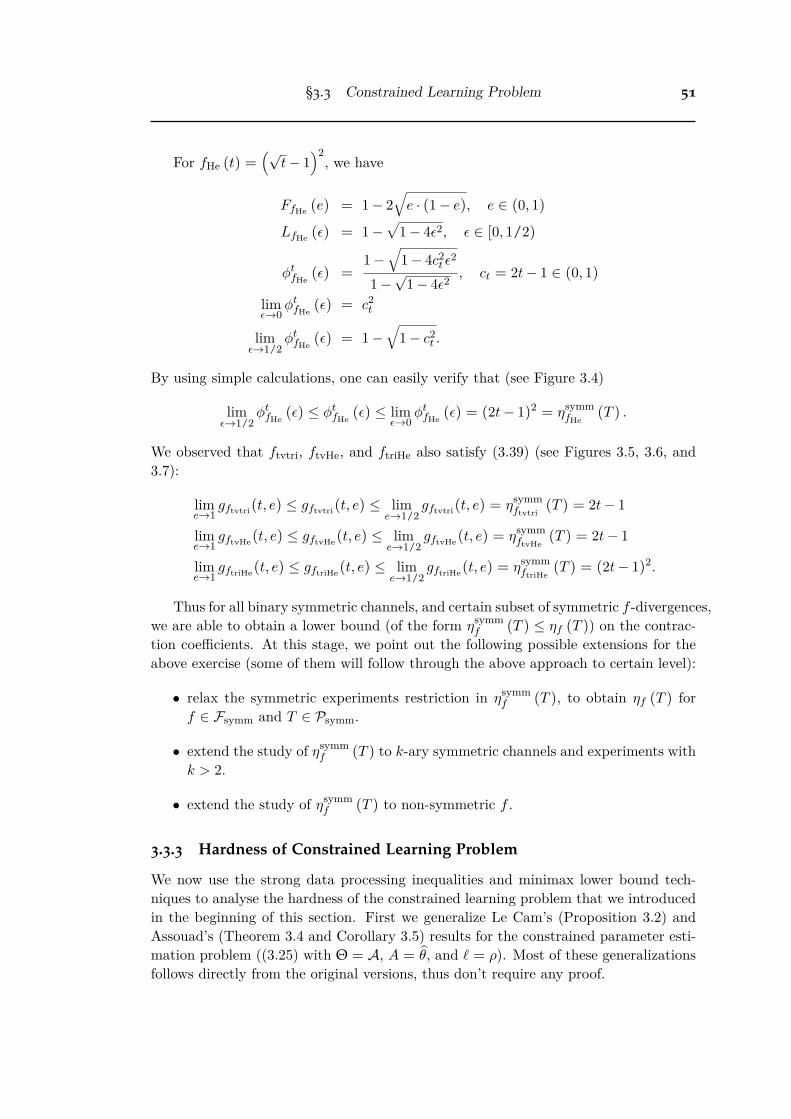
§3.3 Constrained Learning Problem 51
For fHe (t) =1Ô
t ≠ 122
, we have
FfHe (e) = 1 ≠ 2Ò
e · (1 ≠ e), e œ (0, 1)
LfHe (‘) = 1 ≠
1 ≠ 4‘2, ‘ œ [0, 1/2)
„tfHe (‘) =
1 ≠Ò
1 ≠ 4c2t ‘2
1 ≠ Ô1 ≠ 4‘2 , ct = 2t ≠ 1 œ (0, 1)
lim‘æ0
„tfHe (‘) = c2
t
lim‘æ1/2
„tfHe (‘) = 1 ≠
Ò
1 ≠ c2t .
By using simple calculations, one can easily verify that (see Figure 3.4)
lim‘æ1/2
„tfHe (‘) Æ „t
fHe (‘) Æ lim‘æ0
„tfHe (‘) = (2t ≠ 1)2
= ÷symmfHe
(
T)
.
We observed that ftvtri, ftvHe, and ftriHe also satisfy (3.39) (see Figures 3.5, 3.6, and3.7):
limeæ1
gftvtri(t, e) Æ gftvtri(t, e) Æ limeæ1/2
gftvtri(t, e) = ÷symmftvtri
(
T)
= 2t ≠ 1
limeæ1
gftvHe(t, e) Æ gftvHe(t, e) Æ limeæ1/2
gftvHe(t, e) = ÷symmftvHe
(
T)
= 2t ≠ 1
limeæ1
gftriHe(t, e) Æ gftriHe(t, e) Æ limeæ1/2
gftriHe(t, e) = ÷symmftriHe
(
T)
= (2t ≠ 1)2.
Thus for all binary symmetric channels, and certain subset of symmetric f -divergences,we are able to obtain a lower bound (of the form ÷symm
f (
T)
Æ ÷f (T )
) on the contrac-tion coe�cients. At this stage, we point out the following possible extensions for theabove exercise (some of them will follow through the above approach to certain level):
• relax the symmetric experiments restriction in ÷symmf (
T)
, to obtain ÷f (T )
forf œ Fsymm and T œ Psymm.
• extend the study of ÷symmf (
T)
to k-ary symmetric channels and experiments withk > 2.
• extend the study of ÷symmf (
T)
to non-symmetric f .
3.3.3 Hardness of Constrained Learning Problem
We now use the strong data processing inequalities and minimax lower bound tech-niques to analyse the hardness of the constrained learning problem that we introducedin the beginning of this section. First we generalize Le Cam’s (Proposition 3.2) andAssouad’s (Theorem 3.4 and Corollary 3.5) results for the constrained parameter esti-mation problem ((3.25) with Q = A, A =
‚◊, and ¸ = fl). Most of these generalizationsfollows directly from the original versions, thus don’t require any proof.

52 Asymmetric Learning Problems
Figure 3.2: gftv(t, e) of a binary symmetric channel w.r.t. total variation divergence.
Figure 3.3: gftri(t, e) of a binary symmetric channel w.r.t. triangular discriminationdivergence.

§3.3 Constrained Learning Problem 53
Figure 3.4: gfHe(t, e) of a binary symmetric channel w.r.t. symmetric squared Hellingerdivergence (sandwiched according to (3.39)).
Figure 3.5: gftvtri(t, e) of a binary symmetric channel w.r.t. Iftvtri (sandwiched accordingto (3.39)).

54 Asymmetric Learning Problems
Figure 3.6: gftvHe(t, e) of a binary symmetric channel w.r.t. IftvHe (sandwiched accord-ing to (3.39)).
Figure 3.7: gftriHe(t, e) of a binary symmetric channel w.r.t. IftriHe (sandwiched accord-ing to (3.39)).

§3.3 Constrained Learning Problem 55
Proposition 3.16. For any c œ(
0, 1)
, the minimax risk of the constrained parameterestimation problem ( (3.25) with Q = A, A =
‚◊, and ¸ = fl) is lower bounded as
Rıfl (Án) Ø sup
◊ ”=◊Õ
;
fl(
◊, ◊Õ)
·51
2 ≠ n31
2 ≠ c · c4
≠ Ëc (T )
n · Ifc (Á (◊) , Á(
◊Õ))
6<
.
Proof. From Proposition 3.2, we have that
Rıfl (Án) Ø sup
◊ ”=◊Õ
)
fl(
◊, ◊Õ)
·(
c · c ≠ ·Ifc (Án (◊) , Án (◊Õ)))
*
.
Further from Lemma 2.11, we have that
dTV (
cÁn (◊) , cÁn (◊Õ))
Æ ndTV (
cÁ(
◊)
, cÁ(
◊Õ))
.
Thus we have
Ifc (Án (◊) , Án (◊Õ))
Æ nIfc (Á (◊) , Á(
◊Õ))
+
3
c · c ≠ 12
4
· (1 ≠ n)
Æ Ëc (T )
nIfc (Á (◊) , Á(
◊Õ))
+
3
c · c ≠ 12
4
· (1 ≠ n).
Theorem 3.17. Let Q = {≠1, 1}d and fl = flHa (defined in (2.1)). Then for anyc œ
(
0, 1)
, the minimax risk of the constrained parameter estimation problem ( (3.25)with Q = A, A =
‚◊, and ¸ = fl) is lower bounded as
RıflHa (Án) Ø d
A
c · c ≠ max◊,◊Õ:flHa(◊,◊Õ
)=1Ifc (Án (◊) , Án (◊
Õ))
B
Corollary 3.18. Let O be some set and c œ(
0, 1)
. Define
PÁ (O)
:=Ó
Á(
◊)
œ P(
O)
: ◊ œ {≠1, 1}dÔ
be a class of probability measures induced by the transition Á : {≠1, 1}d O. Supposethat there exists some cost-dependent constant –
(
c)
> 0, such that
He2(
Á(
◊)
, Á(
◊Õ))
Æ –(
c)
, if flHa (◊, ◊Õ)
= 1.
The minimax risk of the constrained parameter estimation problem ( (3.25) with Q = A,A =
‚◊, and ¸ = flHa) is lower bounded as
RıflHa (Án) Ø d · (c · c) ·
3
1 ≠Ò
–(
c)
÷He2 (T )
n4
, (3.41)
where T is as per (3.25) and ÷He2 (T )
is the contraction coe�cient of T w.r.t. squaredHellinger distance.

56 Asymmetric Learning Problems
Proof. For any two ◊, ◊Õ œ Q with flHa (◊, ◊Õ)
= 1, we have
Ifc (Án (◊) , Án (◊Õ))
Æ(
c · c)
· He(
Án (◊) , Án (◊Õ))
Æ(
c · c)
·ˆ
ı
ı
Ù
nÿ
i=1He2
(
Á(
◊)
, Á(
◊Õ))
Æ(
c · c)
·ˆ
ı
ı
Ù
nÿ
i=1÷He2 (T )
He2(
Á(
◊)
, Á(
◊Õ))
Æ(
c · c)
·Ò
–(
c)
÷He2 (T )
n
Consider the corrupted cost-sensitive binary classification problem represented bythe following transition diagram:
Qh,F (
X ◊ {≠1, 1})
n(
X ◊ {≠1, 1})
n FÁn T1:n‚f
,(3.42)
and the minimax risk of it given by
RıD¸dc
(
Án) := inf‚f
sup◊œQh,F
E{(Xi,Yi)}n
i=1≥Án(◊)
S
U Ef≥‚f
(
{(Xi,Yi)}ni=1)
[
D¸dc (◊, f)]
T
V. (3.43)
Theorem 3.19. Let F be a VC class of binary-valued functions on X with VC dimen-sion V Ø 2. Then for any n Ø V and any h œ [0, c · c], the minimax risk (3.43) of thecorrupted cost-sensitive binary classification (3.42) is lower bounded as follows:
RıD¸dc
(
Án) Ø K · (c · c) · minA
Û
(c · c)V
÷He2 (T )
n, (c · c) · V
÷He2 (T )
nh
B
where K > 0 is some absolute constant.
The number of samples that appear in the minimax lower bound of the originallearning problem is scaled by the contraction coe�cient ÷f (T ) in the case of corruptedlearning problem. Hence the rate is una�ected, only the constants. However, a penaltyof factor ÷f (T ) is unavoidable no matter what learning algorithm is used, suggestingthat ÷f (T ) is a valid way of measuring the amount of corruption.
3.4 Cost-sensitive Privacy Notions
Suppose a trustworthy data curator gathers sensitive data from a large number of dataproviders, with the goal of learning statistical facts about the underlying population.

§3.4 Cost-sensitive Privacy Notions 57
A data analyst makes a statistical query on the sensitive dataset from the data curator.Thus the main challenge for the data curator is to send back a randomized response suchthat the utility of the task of the data analyst is increased while maintaining the privacyof the data providers. This requires a formal definition of privacy, and di�erentialprivacy has been put forth as such formalization (Dwork et al. [2006]). Di�erentialprivacy requires that the data analyst knows no more about any individual in thesensitive dataset after the analysis is completed, than she knew before the analysis wasbegun. That is the impact on the data provider is the same independent of whether ornot he was in the analysis. It is possible to reduce the problem of enforcing di�erentialprivacy to a statistical decision problem (Wasserman and Zhou [2010]). We exploit thisobservation and extend it further (see section 3.4.2).
In a more restrictive requirement than the di�erential privacy, called “local privacy”([Duchi et al., 2013; Warner, 1965]), the data providers don’t even trust the data curatorcollecting the data. When the sensitive data to be protected is other than the value of asingle individual, it is common to consider di�erent definitions for privacy requirements.
A privacy mechanism is an algorithm that takes as input a database, a universe V ofdata types (of the database), and optionally a set of queries, and produce a randomizedresponse. The privacy mechanism can be represented by a transition T : O ‚O. Belowwe represent some of the privacy enforced settings via transition diagrams:
• We need to protect an abstract set of secrets X (for example geographical lo-cations of army base points) from the data analyst, who wants to learn somesummary statistic about the probability distribution which generated the secretsi.e. something about the actual parameter ◊ from the parameter space Q. Thissetting is represented by the following transition diagram
Q X ZÁ T
, (3.44)
where T is the privacy mechanism and Z is the new outcome space observedby the data analyst. When the outcome space Z = X , the resulting transitiondiagram is
Q X XÁ T
. (3.45)
• We need to protect the entries of the database by releasing a sanitized database(this approach is also referred to as non-interactive method). Let the databaseuniverse be V. Then by repeatedly applying the privacy mechanism T in thetransition diagram (3.45) with X = V, over all the entries of the database, weget
Q Vn VnÁn T1:n
. (3.46)
• In comparison to the above non-interactive approach, it is possible to protectthe entries of the database by corrupting the response for the database query

58 Asymmetric Learning Problems
appropriately. This interactive (query dependent) method can be represented bythe following transition digram
Q X Y ZÁ f H
, (3.47)
where X = Vn is the database (with universe V) to be protected, f is a query onthe database, and H is the privacy mechanism over the query outcome space Y.We need to enforce restrictions on the composite mechanism T = H ¶ f in orderto protect the elements of X . By appropriate tailoring, these restrictions can bereduced to the restrictions on the mechanism H depending on f .
Based on the discussions above, without loss of generality, we only consider the privacydefinitions for the setting represented by the transition diagram (3.44), with finite Xand Z.
3.4.1 Symmetric Local Privacy
First we briefly review the (symmetric) local privacy notion which is well studied in theliterature ([Dwork, 2008; Duchi et al., 2013]). Consider the setting represented by thetransition diagram (3.44) with finite X and Z. The (symmetric) local privacy imposesindistinguishability between pairs of secrets and protects all of them equally:
Definition 3.20 ([Duchi et al., 2013]). Given ‘ > 0, let M(
X , Z; ‘)
™ M(
X , Z)
denote the set of all ‘-locally private mechanisms where
T œ M(
X , Z; ‘)
≈∆ T (z | xi)
T (z | xj)Æ e‘, ’xi, xj œ X , z œ Z. (3.48)
Below we provide a hypothesis testing based interpretation of the above definition,essentially noted by Wasserman and Zhou [2010].
Hypothesis Testing Interpretation: Based on the random outcome in Z from theprivacy mechanism T , we want determine whether it is generated by the secret xi orxj . Let the labels 1 and 0 correspond to the probability measures T
(
xi) and T(
xj)
respectively. Consider a statistical test (recall from section 2.4.1) rij : Z æ {0, 1}.Then the false negative and false positive rates of this test are given by
FNrij :=ÿ
zœZT(
z | xi) Jrij (z) = 0K, and (3.49)
FPrij :=ÿ
zœZT(
z | xj) Jrij (z) = 1K, (3.50)
respectively. The ‘-local privacy condition on a mechanism T is equivalent to thefollowing set of constraints on the false negative and false positive rates:

§3.4 Cost-sensitive Privacy Notions 59
1
1
tı
FP
FN
(a) tı=
! 1e‘+1 , 1
e‘+1
"
1
1
tı
FP
TP
(b) tı
=
! 1e‘+1 , e‘
e‘+1
"
Figure 3.8: Operational characteristic representation of ‘-local privacy mechanisms(with ‘ = 0.7).
Theorem 3.21 ([Kairouz et al., 2014]). For any ‘ > 0, a mechanism T œ M(
X , Z)
is‘-locally private if and only if the following conditions are satisfied for all xi, xj œ X ,and all statistical tests rij : Z æ {0, 1}:
FNrij + e‘ · FPrij Ø 1, (3.51)e‘ · FNrij + FPrij Ø 1. (3.52)
The above operational interpretation says that it is impossible to get both small falsenegative and false positive rates from data obtained via a ‘-locally private mechanism.The above characterization is graphically represented in Figure 3.8, where the shadedregion of the left side diagram (Figure 3.8(a)) can be mathematically written as follows
S(
‘)
:= {(
FP, FN)
: FN + e‘ · FP Ø 1, and e‘ · FN + FP Ø 1} . (3.53)
We define the privacy region of a mechanism T with respect to xi and xj as
S(
T , xi, xj) := conv1Ó1
FPrij , FNrij
2
: for all rij : Z æ {0, 1}Ô2
, (3.54)
where conv(
·)
is the convex hull of a set. The following corollary, which follows imme-diately from Theorem 3.21, gives a necessary and su�cient condition for a mechanismto be ‘-locally private.
Corollary 3.22. A mechanism T is ‘-locally private if and only if S(
T , xi, xj) ™ S(
‘)
for all xi, xj œ X .
3.4.2 Non-homogeneous Local Privacy
Now if we want to protect some secrets more than others we need to break the inherentsymmetry in the privacy definition of the previous section. Here we introduce an
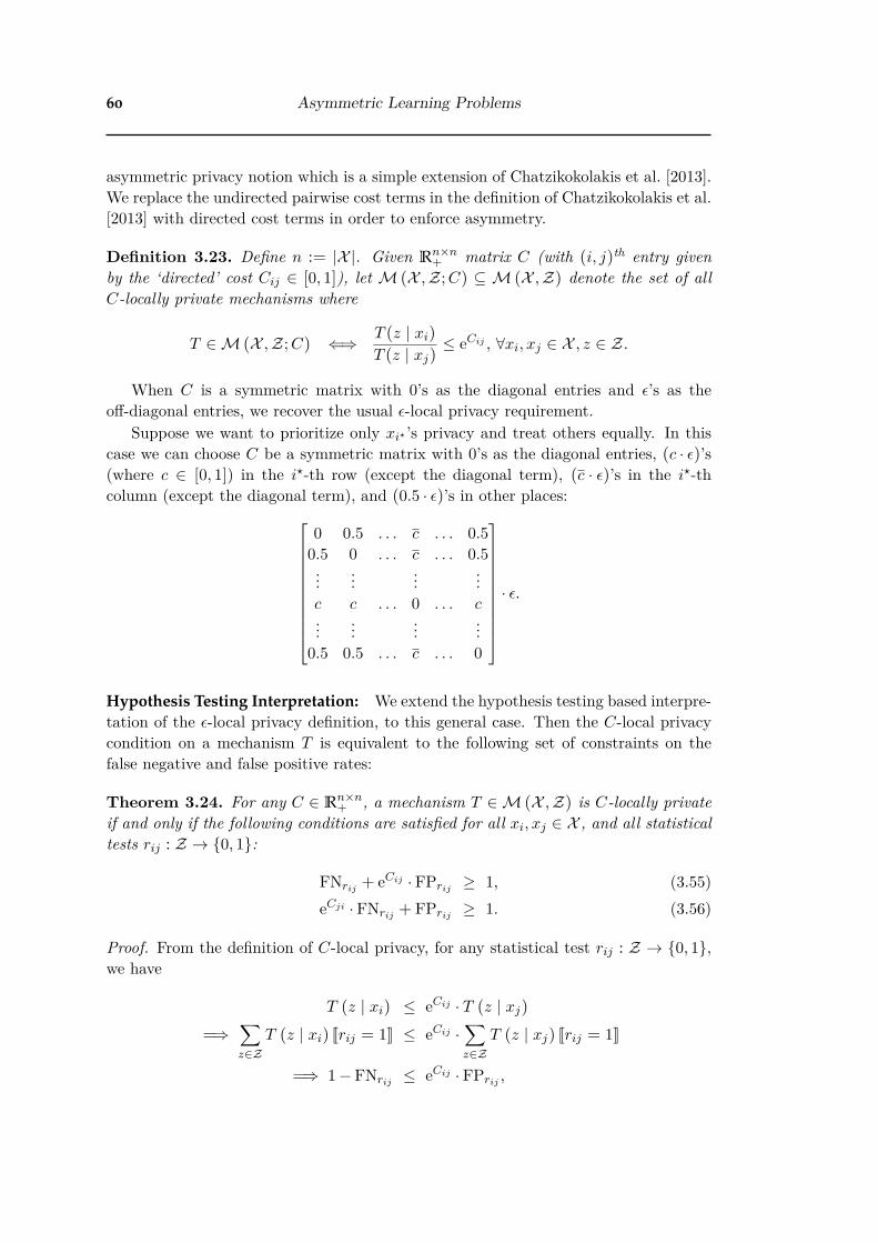
60 Asymmetric Learning Problems
asymmetric privacy notion which is a simple extension of Chatzikokolakis et al. [2013].We replace the undirected pairwise cost terms in the definition of Chatzikokolakis et al.[2013] with directed cost terms in order to enforce asymmetry.
Definition 3.23. Define n := |X |. Given Rn◊n+
matrix C (with (i, j)th entry givenby the ‘directed’ cost Cij œ
[
0, 1]
), let M(
X , Z; C)
™ M(
X , Z)
denote the set of allC-locally private mechanisms where
T œ M(
X , Z; C)
≈∆ T (z | xi)
T (z | xj)Æ eCij , ’xi, xj œ X , z œ Z.
When C is a symmetric matrix with 0’s as the diagonal entries and ‘’s as theo�-diagonal entries, we recover the usual ‘-local privacy requirement.
Suppose we want to prioritize only xiı ’s privacy and treat others equally. In thiscase we can choose C be a symmetric matrix with 0’s as the diagonal entries, (c · ‘)’s(where c œ
[
0, 1]
) in the iı-th row (except the diagonal term), (c · ‘)’s in the iı-thcolumn (except the diagonal term), and (0.5 · ‘)’s in other places:
S
W
W
W
W
W
W
W
W
W
W
U
0 0.5 . . . c . . . 0.50.5 0 . . . c . . . 0.5...
......
...c c . . . 0 . . . c...
......
...0.5 0.5 . . . c . . . 0
T
X
X
X
X
X
X
X
X
X
X
V
· ‘.
Hypothesis Testing Interpretation: We extend the hypothesis testing based interpre-tation of the ‘-local privacy definition, to this general case. Then the C-local privacycondition on a mechanism T is equivalent to the following set of constraints on thefalse negative and false positive rates:
Theorem 3.24. For any C œ Rn◊n+
, a mechanism T œ M(
X , Z)
is C-locally privateif and only if the following conditions are satisfied for all xi, xj œ X , and all statisticaltests rij : Z æ {0, 1}:
FNrij + eCij · FPrij Ø 1, (3.55)eCji · FNrij + FPrij Ø 1. (3.56)
Proof. From the definition of C-local privacy, for any statistical test rij : Z æ {0, 1},we have
T(
z | xi) Æ eCij · T(
z | xj)
=∆ÿ
zœZT(
z | xi) Jrij = 1K Æ eCij ·ÿ
zœZT(
z | xj) Jrij = 1K
=∆ 1 ≠ FNrij Æ eCij · FPrij ,

§3.4 Cost-sensitive Privacy Notions 61
1
1
tıij
FP
FN
(a) tıij = (–, —)
1
1
tıij
FP
TP
(b) tıij = (–, 1 ≠ —)
Figure 3.9: Operational characteristic representation of C-local privacy mechanisms(with Cij = 1.05 and Cji = 0.45). Note that Cij > Cji. Observe that – =
eCji ≠1e(Cij+Cji)≠1
and — =
eCij ≠1e(Cij+Cji)≠1
.
and
T(
z | xj) Æ eCji · T(
z | xi)
=∆ÿ
zœZT(
z | xj) Jrij = 0K Æ eCij ·ÿ
zœZT(
z | xi) Jrij = 0K
=∆ 1 ≠ FPrij Æ eCji · FNrij .
The above characterization is graphically represented in Figure 3.9, where theshaded region of the left side diagram (Figure 3.9(a)) can be mathematically writtenas follows
S(
C, xi, xj) :=Ó
(
FP, FN)
: FN + eCij · FP Ø 1, and eCji · FN + FP Ø 1Ô
. (3.57)
Note that unlike Figure 3.8 which holds ’i ”= j, here in general we get a di�erentpicture for each choice of i and j. The following corollary, which follows immediatelyfrom Theorem 3.24, gives a necessary and su�cient condition on the privacy region forC-local privacy.
Corollary 3.25. A mechanism T is C-locally private if and only if S(
T , xi, xj) ™S(
C, xi, xj) for all xi, xj œ X .
To facilitate the mechanism design, we define the following
S(
C, xi) :=‹
xjœX \xi
S(
C, xi, xj), (3.58)

62 Asymmetric Learning Problems
1
1
tıij
tıik
tıi
FP
FN
(a)
1
1
tıij
tıik
tıi
FP
TP
(b)
Figure 3.10: Feasible region for T(
· | xi) under C-local privacy. The point tıi will
impact the optimal privacy mechanism’s T(
· | xi).
using which we can design T(
· | xi). This is illustrated in Figure 3.10.Figure 3.11 is plotted for two di�erent C: one with Cij = 1.05 and Cji = 0.45, and
the other with Cij = Cji = 0.75. This diagram shows how much we lose by prioritizingsomeone’s privacy than others. It can be observed that the permissible ROC regionfor the privacy mechanism gets shrunk (compared to the equal privacy case) when weenforce prioritized privacy for someone.
3.5 Conclusion
The cost-sensitive classification problem plays a crucial role in mission critical machinelearning applications. We have studied the hardness of this problem and emphasizedthe impact of cost terms on the hardness.
Strong data processing inequalities (SDPI) are very useful in analysing the hard-ness of constrained learning problems. Despite extensive investigation, the geometricinsights of the SDPI are not fully understood. This chapter provides some direction.To this end, we have derived an explicit form for the contraction coe�cient of anychannel w.r.t. c-primitive f -divergence, and we have obtained e�ciently computablelower bound for the contraction coe�cient of any binary symmetric channel w.r.t. anysymmetric f -divergence.
We pose the following open problems as future directions:
• There are some divergences other than f -divergences which satisfy the weak dataprocessing inequality, such as Neyman-Pearson –-divergences ([Polyanskiy andVerdú, 2010; Raginsky, 2011]). Thus it would be interesting to study strong dataprocessing inequalities w.r.t. those divergences as well.
• Recently people have attempted to relate several types of channel ordering to thestrong data processing inequalities ([Makur and Polyanskiy, 2016; Polyanskiy

§3.6 Appendix 63
1
1
tıij
tıji
tı
FP
TP
Figure 3.11: Comparison between ‘-local privacy (with ‘ = 0.75) and C-local privacy(with Cij = 1.05, and Cji = 0.45).
and Wu, 2015]). It would be interesting to study the relationship between thestatistical deficiency based channel ordering (Raginsky [2011]) and the strongdata processing inequalities.
• Wider exploration of asymmetric privacy notions.
3.6 Appendix
3.6.1 VC Dimension
A measure of complexity in learning theory should reflect which learning problems areinherently easier than others. The standard approach in statistical theory is to definethe complexity of the learning problem through some notion of “richness”, “size”,“capacity” of the hypothesis class.
The complexity measure proposed in Vapnik and Chervonenkis [1971], the Vapnik-Chervonenkis (VC) dimension is a combinatorial measure of the richness of classes ofbinary-valued functions when evaluated on samples. VC-dimension is independent ofthe underlying probability measure and of the particular sample, and hence is worst-case estimate with regard to these quantities.
We use the notation xm1 for a sequence
(
x1, . . . , xm)
œ X m, and for a class ofbinary-valued functions F ™ {≠1, 1}X , we denote by F|xm
1the restriction of F to xm
1 :
F|xm1= {
(
f(
x1) , . . . , f(
xm))
| f œ F} .
Define the m-th shatter coe�cient of F as follows:
Sm (
F)
:= maxxm
1 œX m|F|xm
1|.

64 Asymmetric Learning Problems
Definition 3.26. Let F ™ {≠1, 1}X and let xm1 =
(
x1, . . . , xm)
œ X m. We say xm1 is
shattered by F if |F|xm1
| = 2m; i.e. if ’b œ {≠1, 1}m, ÷fb œ F s.t.(
fb (
x1) , . . . , fb (
xm))
=
b. The Vapnik-Chervonenkis (VC) dimension of F , denoted by VCdim(
F)
, is the car-dinality of the largest set of points in X that can be shattered by F :
VCdim(
F)
= max {m œ N | Sm (
F)
= 2m}.
If F shatters arbitrarily large sets of points in X , then VCdim(
F)
= Œ. If VCdim(
F)
<Œ, we say that F is a VC class.

Chapter 4
Exp-concavity of ProperComposite Losses
Loss functions are the means by which the quality of a prediction in learning problem isevaluated. A composite loss (the composition of a class probability estimation (CPE)loss with an invertible link function which is essentially just a re-parameterization) isproper if its risk is minimized when predicting the true underlying class probability (aformal definition is given later). In Williamson et al. [2016], there is an argument thatshows that there is no point in using losses that are neither proper nor proper compositeas they are inadmissible. Flexibility in the choice of loss function is important to tailorthe solution to a learning problem (Buja et al. [2005], Hand [1994], Hand and Vinciotti[2003]), and it could be attained by characterizing the set of loss functions using naturalparameterizations.
The goal of the learner in a game of prediction with expert advice (which is formallydescribed in section 4.1.5) is to predict as well as the best expert in the given poolof experts. The regret bound of the learner depends on the merging scheme usedto merge the experts’ predictions and the type of loss function used to measure theperformance. It has already been shown that constant regret bounds are achievable formixable losses when the Aggregating Algorithm is the merging scheme (Vovk [1995]),and for exp-concave losses when the Weighted Average Algorithm is the merging scheme(Kivinen and Warmuth [1999]). We can see that the exp-concavity trivially impliesmixability. Even though the converse implication is not true in general, under somere-parameterization we can make it possible. This chapter discusses general conditionson proper losses under which they can be transformed to an exp-concave loss through asuitable link function. In the binary case, these conditions give two concrete formulas(Proposition 4.1 and Corollary 4.8) for link functions that can transform —-mixableproper losses into —-exp-concave, proper, composite losses. The explicit form of thelink function given in Proposition 4.1 is derived using the same geometric constructionused in van Erven [2012].
Further we extend the work by Williamson et al. [2016], to provide a completecharacterization of the exp-concavity of the proper composite multi-class losses in termsof the Bayes risk associated with the underlying proper loss, and the link function.The mixability of proper losses (mixability of a proper composite loss is equivalent
65

66 Exp-concavity of Proper Composite Losses
to the mixability of its generating proper loss) is studied in Van Erven et al. [2012].Using these characterizations (for the binary case), in Corollary 4.8 we derive an exp-concavifying link function that can also transform any —-mixable proper loss into a—-exp-concave composite loss. Since for the multi-class losses these conditions do nothold in general, we propose a geometric approximation approach (Proposition 4.2)which takes a parameter ‘ and transforms the mixable loss function appropriately ona subset S‘ of the prediction space. When the prediction space is Dn, any predictionbelongs to the subset S‘ for su�ciently small ‘. In the conclusion we provide a wayto use the Weighted Average Algorithm with learning rate — for proper —-mixable butnon-exp-concave loss functions to achieve O(1) regret bound.
The exp-concave losses achieve O(log T ) regret bound in online convex optimizationalgorithms, which is a more general setting of online learning problems. Thus the exp-concavity characterization of composite losses could be helpful in constructing exp-concave losses for online learning problems.
The chapter is organized as follows. In Section 4.1 we formally introduce the lossfunction, several loss types, conditional risk, proper composite losses and a game of pre-diction with expert advice. In Section 4.2 we consider our main problem — whetherone can always find a link function to transform —-mixable losses into —-exp-concavelosses. Section 4.3 concludes with a brief discussion. The impact of the choice of sub-stitution function on the regret of the learner is explored via experiments in Appendix4.4.1. In Appendix 4.4.2, we discuss the mixability conditions of probability games withcontinuous outcome space. Detailed proofs are in Appendix 4.4.3.
4.1 Preliminaries and Background
This section provides the necessary background on loss functions, conditional risks,and the sequential prediction problem.
4.1.1 Notation
We use the following notation throughout this chapter. A superscript prime, AÕ denotestranspose of the matrix or vector A, except when applied to a real-valued functionwhere it denotes derivative (f Õ). We denote the matrix multiplication of compatiblematrices A and B by A · B, so the inner product of two vectors x, y œ Rn is xÕ · y.Let [n] := {1, ..., n}, R
+
:= [0, Œ) and the n-simplex Dn := {(p1, ..., pn)Õ : 0 Æ pi Æ
1, ’i œ [n], andq
iœ[n] pi = 1}. If x is a n-vector, A = diag(x) is the n ◊ n matrixwith entries Ai,i = xi , i œ [n] and Ai,j = 0 for i ”= j. If A ≠ B is positive definite(resp. semi-definite), then we write A º B (resp. A < B). We use en
i to denotethe ith n-dimensional unit vector, en
i = (0, ..., 0, 1, 0, ...0)Õ when i œ [n], and defineen
i = 0n when i > n. The n-vector 1n := (1, ..., 1)Õ. We write JP K = 1 if P is trueand JP K = 0 otherwise. Given a set S and a weight vector w, the convex combinationof the elements of the set w.r.t the weight vector is denoted by cowS, and the convexhull of the set which is the set of all possible convex combinations of the elements ofthe set is denoted by coS (Rockafellar [1970]). If S, T µ Rn, then the Minkowski sum
§4.1 Preliminaries and Background 67
S � T := {s + t : s œ S, t œ T}. YX represents the set of all functions f : X æ Y. Wesay f : C µ Rn æ Rn is monotone (resp. strictly monotone) on C when for all x andy in C,
(f(x) ≠ f(y))Õ · (x ≠ y) Ø 0 resp. (f(x) ≠ f(y))Õ · (x ≠ y) > 0;
confer Hiriart-Urruty and Lemaréchal [1993]. Other notation (the Kronecker product¢, the Jacobian D, and the Hessian H) is defined in Appendix A of Van Erven et al.[2012]. Df(v) and Hf(v) denote the Jacobian and Hessian of f(v) w.r.t. v respectively.When it is not clear from the context, we will explicitly mention the variable; forexample Dvf(v) where v = h(v).
4.1.2 Loss Functions
For a prediction problem with an instance space X , outcome space Y and predictionspace V, a loss function ¸ : Y ◊ V æ R
+
(bivariate function representation) can bedefined to assign a penalty ¸(y, v) for predicting v œ V when the actual outcome isy œ Y. When the outcome space Y = [n], n Ø 2, the loss function ¸ is called a multi-class loss and it can be expressed in terms of its partial losses ¸i := ¸(i, ·) for anyoutcome i œ [n], as
¸(y, v) =ÿ
iœ[n]Jy = iK¸i(v).
The vector representation of the multi-class loss is given by ¸ : V æ Rn+
, which assignsa vector ¸(v) = (¸1(v), ..., ¸n(v))Õ to each prediction v œ V. A loss is di�erentiable if allof its partial losses are di�erentiable. In this thesis, we will use the bivariate functionrepresentation (¸(y, v)) to denote a general loss function and the vector representationfor multi-class loss functions.
The super-prediction set of a binary loss ¸ is defined as
S¸ := {x œ Rn : ÷v œ V, x Ø ¸(v)},
where inequality is component-wise. For any dimension n and — Ø 0, the —-exponentialoperator E— : [0, Œ]
n æ [0, 1]n is defined by
E—(x) := (e≠—x1 , ..., e≠—xn)
Õ.
For — > 0 it is clearly invertible with inverse
E≠1— (z) = ≠—≠1
(ln z1, ..., ln zn)Õ.
The —-exponential transformation of the super-prediction set is given by
E—(S¸) := {(e≠—x1 , ..., e≠—xn)
Õ œ Rn : (x1, ..., xn)Õ œ S¸}, — > 0.
A multi-class loss ¸ is
• convex if f(v) = ¸y(v) is convex in v for all y œ [n],

68 Exp-concavity of Proper Composite Losses
• –-exp-concave (for – > 0) if f(v) = e≠–¸y(v) is concave in v for all y œ [n](Cesa-Bianchi and Lugosi [2006]),
• weakly mixable if the super-prediction set S¸ is convex (Kalnishkan and Vyugin[2005]), and
• —-mixable (for — > 0) if the set E—(S¸) is convex (Vovk and Zhdanov [2009]; Vovk[1995]).
The mixability constant —¸ of a loss ¸ is the largest — such that ¸ is —-mixable; i.e.
—¸ := sup {— > 0 : ¸ is —-mixable}.
If the loss function ¸ is –-exp-concave (resp. —-mixable) then it is –Õ-exp-concave forany 0 < –Õ Æ – (resp. —Õ-mixable for any 0 < —Õ Æ —), and its ⁄-scaled version (⁄¸) forsome ⁄ > 0 is –
⁄ -exp-concave (resp. —⁄ -mixable). If the loss ¸ is –-exp-concave, then it
is convex and –-mixable (Cesa-Bianchi and Lugosi [2006]).For a multi-class loss ¸, if the prediction space V = Dn then it is said to be multi-
class probability estimation (CPE) loss, where the predicted values are directly inter-preted as probability estimates: ¸ : Dn æ Rn
+
. We will say a multi-CPE loss is fairwhenever ¸i(en
i ) = 0, for all i œ [n]. That is, there is no loss incurred for perfectprediction. Examples of multi-CPE losses include
1. the square loss ¸sqi (q) :=
q
jœ[n](Ji = jK ≠ qj)2,
2. the log loss ¸logi (q) := ≠ log qi,
3. the absolute loss ¸absi (q) :=
q
jœ[n] |Ji = jK ≠ qj |, and
4. the 0-1 loss ¸01i (q) := Ji /œ arg maxjœ[n] qjK.
4.1.3 Conditional and Full Risks
Let X and Y be random variables taking values in the instance space X and the outcomespace Y = [n] respectively. Let D be the joint distribution of (X, Y) and for x œ X ,denote the conditional distribution by p(x) = (p1(x), ..., pn(x))Õ where pi(x) := P (Y =
i|X = x), ’i œ [n], and the marginal distribution by M (x) := P (X = x). For anymulti-CPE loss ¸, the conditional Bayes risk is defined as
L¸ : Dn ◊ Dn – (p, q) ‘æ L¸(p, q) = EY≥p[¸Y(q)] = pÕ · ¸(q) =ÿ
iœ[n]pi¸i(q) œ R
+
, (4.1)
where Y ≥ p represents a Multinomial distribution with parameter p œ Dn. The fullBayes risk of the estimator function q : X æ Dn is defined as
‚R¸(M , p, q) := E(X,Y)≥D[¸Y(q(X))] = EX≥M [L¸(p(X), q(X))].
§4.1 Preliminaries and Background 69
Furthermore the minimum full Bayes risk is defined as
‚R¸(M , p) := infqœ(Dn
)
X‚R¸(M , p, q) = EX≥M [L¸(p(X))],
where L¸(p) = infqœDn L¸(p, q) is the minimum conditional Bayes risk and is alwaysconcave (Gneiting and Raftery [2007]). If ¸ is fair, L¸(e
ni ) = ¸i(en
i ) = 0. One canunderstand the e�ect of choice of loss in terms of the conditional perspective (Reid andWilliamson [2011]), which allows one to ignore the marginal distribution M of X whichis typically unknown.
4.1.4 Proper and Composite Losses
A multi-CPE loss ¸ : Dn æ Rn+
is said to be proper if for all p œ Dn, L¸(p) =
L¸(p, p) = pÕ · ¸(p) (Buja et al. [2005], Gneiting and Raftery [2007]), and strictly properif L¸(p) < L¸(p, q) for all p, q œ Dn and p ”= q. It is easy to see that the log loss, squareloss, and 0-1 loss are proper while absolute loss is not. Furthermore, both log loss andsquare loss are strictly proper while 0-1 loss is proper but not strictly proper.
Given a proper loss ¸ : Dn æ Rn+
with di�erentiable Bayes conditional risk L¸ :Dn ‘æ R
+
, in order to be able to calculate derivatives easily, following Van Erven et al.[2012] we define
Dn :=I
(p1, . . . , pn≠1)Õ : pi Ø 0,
n≠1ÿ
i=1pi Æ 1
J
(4.2)
PD : Rn+
– p = (p1, . . . , pn)Õ ‘æ p = (p1, . . . , pn≠1)
Õ œ Rn≠1+
(4.3)
P≠1D : Dn – p = (p1, . . . , pn≠1)
Õ ‘æ p = (p1, . . . , pn≠1, 1 ≠ÿn≠1
i=1pi)
Õ œ Dn (4.4)
L¸ : Dn – p ‘æ L¸(P≠1D (p)) œ R
+
(4.5)˜ : Dn – p ‘æ PD(¸(P≠1
D (p))) œ Rn≠1+
. (4.6)
Let  : Dn æ V ™ Rn≠1+
be continuous and strictly monotone (hence invertible) forsome convex set V. It induces  : Dn æ V via
 :=  ¶ PD. (4.7)
Clearly  is continuous and invertible with Â≠1= P≠1
D ¶ Â≠1. We can now extendthe notion of properness to the prediction space V from Dn using this link function.Given a proper loss ¸ : Dn æ Rn
+
, a proper composite loss ¸Â : V æ Rn+
for multi-classprobability estimation is defined as ¸Â := ¸ ¶ Â≠1
= ¸ ¶ P≠1D ¶ Â≠1. We can easily see
that the conditional Bayes risks of the composite loss ¸Â and the underlying proper loss¸ are equal (L¸ = L¸Â ). Every continuous proper loss has a convex super-predictionset (Williamson et al. [2016]). Thus they are weakly mixable. Since by applying a linkfunction the super-prediction set won’t change (as it is just a re-parameterization), allproper composite losses are also weakly mixable.

70 Exp-concavity of Proper Composite Losses
4.1.5 Game of Prediction with Expert Advice
Let Y be the outcome space, V be the prediction space, and ¸ : Y ◊ V æ R+
be theloss function, then a game of prediction with expert advice represented by the tuple(Y, V, ¸) can be described as follows: for each trial t = 1, ..., T ,
• N experts make their prediction v1t , ..., vN
t œ V• the learner makes his own decision vt œ V• the environment reveals the actual outcome yt œ Y
Let S = (y1, ..., yT ) be the outcome sequence in T trials. Then the cumulative lossof the learner over S is given by LS,¸ :=
qTt=1 ¸(yt, vt), of the i-th expert is given by
LiS,¸ :=
qTt=1 ¸(yt, vi
t), and the regret of the learner is given by RS,¸ := LS,¸ ≠ mini LiS,¸.
The goal of the learner is to predict as well as the best expert; to which end the learnertries to minimize the regret.
When using the exponential weights algorithm (which is an important family ofalgorithms in game of prediction with expert advice), at the end of each trial, theweight of each expert is updated as wi
t+1 _ wit · e≠÷¸(yt,vi
t) for all i œ [N ], where ÷ isthe learning rate and wi
t is the weight of the ith expert at time t (the weight vectorof experts at time t is denoted by wt = (w1
t , ..., wNt )
Õ). Then based on the weightsof experts, their predictions are merged using di�erent merging schemes to make thelearner’s prediction. The Aggregating Algorithm and the Weighted Average Algorithmare two important algorithms in the family of exponential weights algorithm.
Consider multi-class games with outcome space Y = [n]. In the Aggregating Algo-rithm with learning rate —, first the loss vectors of the experts and their weights areused to make a generalized prediction gt = (gt(1), ..., gt(n))Õ which is given by
gt := E≠1—
1
cowt{E—
1
(¸1(vit), ..., ¸n(v
it))
Õ2}iœ[N ]
2
= E≠1—
Q
a
ÿ
iœ[N ]
wit(e
≠—¸1(vit), ..., e≠—¸n(vi
t))
ÕR
b .
Then this generalized prediction is mapped into a permitted prediction vt via a sub-stitution function such that (¸1(vt), ..., ¸n(vt))
Õ Æ c(—)(gt(1), ..., gt(n))Õ, where the in-equality is element-wise and the constant c(—) depends on the learning rate. If ¸ is—-mixable, then E—(S¸) is convex, so co{E— (¸(v)) : v œ V} ™ E—(S¸), and we can al-ways choose a substitution function with c(—) = 1. Consequently for —-mixable losses,the learner of the Aggregating Algorithm is guaranteed to have regret bounded by log N
—(Vovk [1995]).
In the Weighted Average Algorithm with learning rate –, the experts’ predic-tions are simply merged according to their weights to make the learner’s predictionvt = cowt{vi
t}iœ[N ]
, and this algorithm is guaranteed to have a log N– regret bound for
–-exp-concave losses (Kivinen and Warmuth [1999]). In either case it is preferred tohave bigger values for the constants — and – to have better regret bounds. Since an–-exp-concave loss is —-mixable for some — Ø –, the regret bound of the Weighted
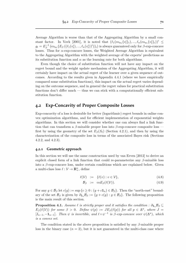
§4.2 Exp-Concavity of Proper Composite Losses 71
Average Algorithm is worse than that of the Aggregating Algorithm by a small con-stant factor. In Vovk [2001], it is noted that (¸1(cowt{vi
t}i), ..., ¸n(cowt{vit}i))
Õ Ægt = E≠1
—
!
cowt{E—!
(¸1(vit), ..., ¸n(vi
t))Õ"}i
"
is always guaranteed only for —-exp-concavelosses. Thus for –-exp-concave losses, the Weighted Average Algorithm is equivalentto the Aggregating Algorithm with the weighted average of the experts’ predictions asits substitution function and – as the learning rate for both algorithms.
Even though the choice of substitution function will not have any impact on theregret bound and the weight update mechanism of the Aggregating Algorithm, it willcertainly have impact on the actual regret of the learner over a given sequence of out-comes. According to the results given in Appendix 4.4.1 (where we have empiricallycompared some substitution functions), this impact on the actual regret varies depend-ing on the outcome sequence, and in general the regret values for practical substitutionfunctions don’t di�er much — thus we can stick with a computationally e�cient sub-stitution function.
4.2 Exp-Concavity of Proper Composite Losses
Exp-concavity of a loss is desirable for better (logarithmic) regret bounds in online con-vex optimization algorithms, and for e�cient implementation of exponential weightsalgorithms. In this section we will consider whether one can always find a link func-tion that can transform a —-mixable proper loss into —-exp-concave composite loss —first by using the geometry of the set E—(S¸) (Section 4.2.1), and then by using thecharacterization of the composite loss in terms of the associated Bayes risk (Sections4.2.2, and 4.2.3).
4.2.1 Geometric approach
In this section we will use the same construction used by van Erven [2012] to derive anexplicit closed form of a link function that could re-parameterize any —-mixable lossinto a —-exp-concave loss, under certain conditions which are explained below. Givena multi-class loss ¸ : V æ Rn
+
, define
¸(V) := {¸(v) : v œ V}, (4.8)B— := coE—(¸(V)). (4.9)
For any g œ B— let c(g) := sup {c Ø 0 : (g + c1n) œ B—}. Then the “north-east” bound-ary of the set B— is given by ˆ1nB— := {g + c(g) : g œ B—}. The following propositionis the main result of this section.Proposition 4.1. Assume ¸ is strictly proper and it satisfies the condition : ˆ1nB— ™E—(¸(V)) for some — > 0. Define Â(p) := JE—(¸(p)) for all p œ Dn, where J =
[In≠1, ≠1n≠1]. Then  is invertible, and ¸ ¶ Â≠1 is —-exp-concave over Â(Dn), which
is a convex set.The condition stated in the above proposition is satisfied by any —-mixable proper
loss in the binary case (n = 2), but it is not guaranteed in the multi-class case where

72 Exp-concavity of Proper Composite Losses
A
B
C
Figure 4.1: Ray “escaping”in 1n direction. More evi-dence in Figure 4.12 in Ap-pendix 4.4.4.
Figure 4.2: Adding “faces”to block rays in (almost)all positive directions.
1
1 O
Figure 4.3: Sub-exp-prediction set extended byremoving near axis-parallelsupporting hyperplanes.
n > 2. In the binary case the link function can be given as Â(p) = e≠—¸1(p) ≠ e≠—¸2(p)
for all p œ D2.Unfortunately, the condition that ˆ1nB— ™ E—(¸(V)) is generally not satisfied;
an example based on squared loss (— = 1 and n = 3 classes) is shown in Figure4.1, where for A and B in E—(¸(V)), the mid-point C can travel along the ray ofdirection 13 without hitting any point in the exp-prediction set E—(¸(V)). Thereforewe resort to approximating a given —-mixable loss by a sequence of —-exp-concave lossesparameterised by positive constant ‘, while the approximation approaches the originalloss in some appropriate sense as ‘ tends to 0. Without loss of generality, we assumeV = Dn.
Inspired by Proposition 4.1, a natural idea to construct the approximation is byadding “faces” to the exp-prediction set such that all rays in the 1n direction willbe blocked. Technically, it turns out more convenient to add faces that block raysin (almost) all directions of positive orthant. See Figure 4.2 for an illustration. Inparticular, we extend the “rim” of the exp-prediction set by hyperplanes that are ‘close to axis-parallel. The key challenge underlying this idea is to design an appropriateparameterisation of the surrogate loss ˜‘, which not only produces such an extendedexp-prediction set, but also ensures that ˜‘(p) = ¸(p) for almost all p œ Dn as ‘ ¿ 0.
Given a —-mixable loss ¸, its sub-exp-prediction set defined as follows must beconvex:
T¸ := E—(¸(Dn))� Rn
≠ = {E—(¸(p)) ≠ x : p œ Dn, x œ Rn+
}. (4.10)
Note T¸ extends infinitely in any direction p œ Rn≠. Therefore it can be written interms of supporting hyperplanes as
T¸ =‹
pœDn
H“p≠p, where “p = min
xœT¸
xÕ · (≠p), and H“p≠p := {x : xÕ · (≠p) Ø “p}. (4.11)
To extend the sub-exp-prediction set with “faces”, we remove some hyperplanes in-volved in (4.11) that correspond to the ‘ “rim” of the simplex (see Figure 4.3 for an

§4.2 Exp-Concavity of Proper Composite Losses 73
illustration in 2-D)
T ‘¸ :=
‹
pœDn‘
H“p≠p, where Dn
‘ := {p œ Dn : mini
pi > ‘}. (4.12)
Since ‘ > 0, for any p œ Dn‘ , E≠1
— (H“p≠p fl Rn
+
) is exactly the super-prediction setof a log-loss with appropriate scaling and shifting (see proof in Appendix 4.4.3). So itmust be convex. Therefore E≠1
— (T ‘¸ fl Rn
+
) =
u
pœDn‘
E≠1— (H
“p≠p fl Rn
+
) must be convex,and its recession cone is clearly Rn
+
. This guarantees that the following loss is properover p œ Dn [Williamson, 2014, Proposition 2]:
˜‘(p) = arg minzœE≠1
— (T ‘¸ flRn
+
)
pÕ · z, (4.13)
where the argmin must be attained uniquely (Appendix 4.4.3). Our next propositionstates that ˜‘ meets all the requirements of approximation suggested above.
Proposition 4.2. For any ‘ > 0, ˜‘ satisfies the condition ˆ1nB— ™ E—(¸(V)). Inaddition, ˜‘ = ¸ over a subset S‘ ™ Dn, where for any p in the relative interior of Dn,p œ S‘ for su�ciently small ‘ i.e. lim‘¿0 vol(Dn \ S‘) = 0.
Note Î ˜‘(p)≠ ¸(p)Î is not bounded for p /œ S‘. While the result does not show thatall —-mixable losses can be made —-exp-concave, it is suggestive that such a result maybe obtainable by a di�erent argument.
4.2.2 Calculus approach
Proper composite losses are defined by the proper loss ¸ and the link Â. In this sectionwe will characterize the exp-concave proper composite losses in terms of (HL¸(p), DÂ(p)).The following proposition provides the identities of the first and second derivatives ofthe proper composite losses (Williamson et al. [2016]).
Proposition 4.3. For all i œ [n], p œ ˚Dn (the interior of Dn), and v = Â(p) œ V ™Rn≠1
+
(so p = Â≠1(v)),
D¸Âi (v) = ≠(en≠1
i ≠ p)Õ · k(p), (4.14)H¸Â
i (v) = ≠1
(en≠1i ≠ p)Õ ¢ In≠1
2
· Dv[k(p)] + k(p)Õ · [DÂ(p)]≠1, (4.15)
wherek(p) := ≠HL¸(p) · [DÂ(p)]≠1. (4.16)
The term k(p) can be interpreted as the curvature of the Bayes risk function L¸
relative to the rate of change of the link function Â. In the binary case where n = 2,above proposition reduces to
(¸Â1 )
Õ(v) = ≠(1 ≠ p)k(p) ; (¸Â
2 )Õ(v) = pk(p), (4.17)
(¸Â1 )
ÕÕ(v) =
≠(1 ≠ p)kÕ(p) + k(p)
ÂÕ(p)
, (4.18)

74 Exp-concavity of Proper Composite Losses
(¸Â2 )
ÕÕ(v) =
pkÕ(p) + k(p)
ÂÕ(p)
, (4.19)
where k(p) =≠L
ÕÕ¸ (p)
ÂÕ(p)
Ø 0 and so ddv k(p) = d
dpk(p) · ddv p =
kÕ(p)
ÂÕ(p)
.A loss ¸ : Dn æ Rn
+
is –-exp-concave (i.e. Dn – q ‘æ ¸y(q) is –-exp-concave for ally œ [n]) if and only if the map Dn – q ‘æ L¸(p, q) = pÕ · ¸(q) is –-exp-concave for allp œ Dn. It can be easily shown that the maps v ‘æ ¸Â
y (v) are –-exp-concave if and onlyif H¸Â
y (v) < –D¸Ây (v)
Õ · D¸Ây (v). By applying Proposition 4.3 we obtain the following
characterization of the –-exp-concavity of the composite loss ¸Â.
Proposition 4.4. A proper composite loss ¸Â= ¸ ¶ Â≠1 is –-exp-concave (with – > 0
and v = Â(p)) if and only if for all p œ ˚Dn and for all i œ [n]
1
(en≠1i ≠ p)Õ ¢ In≠1
2
·Dv[k(p)] 4 k(p)Õ · [DÂ(p)]≠1 ≠–k(p)Õ · (en≠1i ≠ p) · (en≠1
i ≠ p)Õ ·k(p).(4.20)
Based on this characterization, we can determine which loss functions can be exp-concavified by a chosen link function and how much a link function can exp-concavifya given loss function. In the binary case (n = 2), the above proposition reduces to thefollowing.
Proposition 4.5. Let  : [0, 1] æ V ™ R be an invertible link and ¸ : D2 æ R2+
be astrictly proper binary loss with weight function w(p) := ≠HL¸(p) = ≠L
ÕÕ¸ (p). Then the
binary composite loss ¸Â := ¸ ¶ P≠1D ¶ Â≠1 is –-exp-concave (with – > 0) if and only if
≠ 1p+ –w(p)p Æ wÕ
(p)
w(p)≠ ÂÕÕ
(p)
ÂÕ(p)
Æ 11 ≠ p
≠ –w(p)(1 ≠ p), ’p œ (0, 1). (4.21)
The following proposition gives an easier to check necessary condition for the binaryproper losses that generate an –-exp-concave (with – > 0) binary composite loss givena particular link function. Since scaling a loss function will not a�ect what a sensiblelearning algorithm will do, it is possible to normalize the loss functions by normalizingtheir weight functions by setting w(
12 ) = 1. By this normalization we are scaling the
original loss function by 1w(
12 )
and the super-prediction set is scaled by the same factor.If the original loss function is —-mixable (resp. –-exp-concave), then the normalizedloss function is —w(
12 )-mixable (resp. –w(
12 )-exp-concave).
Proposition 4.6. Let  : [0, 1] æ V ™ R be an invertible link and ¸ : D2 æ R2+
be a strictly proper binary loss with weight function w(p) := ≠HL¸(p) = ≠LÕÕ¸ (p)
normalised such that w(
12 ) = 1. Then the binary composite loss ¸Â := ¸ ¶ P≠1
D ¶ Â≠1 is–-exp-concave (with – > 0) only if
ÂÕ(p)
p(2ÂÕ(
12 ) ≠ –(Â(p) ≠ Â( 1
2 )))Q w(p) Q ÂÕ
(p)
(1 ≠ p)(2ÂÕ(
12 ) + –(Â(p) ≠ Â( 1
2 ))), ’p œ (0, 1),
(4.22)where Q denotes Æ for p Ø 1
2 and denotes Ø for p Æ 12 .

§4.2 Exp-Concavity of Proper Composite Losses 75
Figure 4.4: Necessary but not su�cient region of normalised weight functions to ensure–-exp-concavity and convexity of proper losses (— – = 4; — – = 2; — convexity).
Proposition 4.5 provides necessary and su�cient conditions for the exp-concavityof binary composite losses, whereas Proposition 4.6 provides simple necessary but notsu�cient conditions. By setting – = 0 in all the above results we have obtained for exp-concavity, we recover the convexity conditions for proper and composite losses whichare already derived by Reid and Williamson [2010] for the binary case and Williamsonet al. [2016] for multi-class.
4.2.3 Link functions
A proper loss can be exp-concavified (– > 0) by some link function only if the loss ismixable (—¸ > 0) and the maximum possible value for exp-concavity constant is themixability constant of the loss (since the link function won’t change the super-predictionset and an –-exp-concave loss is always —-mixable for some — Ø –).
By applying the identity link Â(p) = p in (4.21) we obtain the necessary andsu�cient conditions for a binary proper loss to be –-exp-concave (with – > 0) as givenby,
≠ 1p+ –w(p)p Æ wÕ
(p)
w(p)Æ 1
1 ≠ p≠ –w(p)(1 ≠ p), ’p œ (0, 1). (4.23)
By substituting Â(p) = p in (4.22) we obtain the following necessary but not su�cient(simpler) constraints for a normalized binary proper loss to be –-exp-concave
1p(2 ≠ –(p ≠ 1
2 ))Q w(p) Q 1
(1 ≠ p)(2 + –(p ≠ 12 ))
, ’p œ (0, 1), (4.24)

76 Exp-concavity of Proper Composite Losses
Figure 4.5: Necessary and su�cient region of unnormalised weight functions to ensure–-exp-concavity of composite losses with canonical link (— – = 2; — – = 4; — – = 8).
which are illustrated as the shaded region in Figure 4.4 for di�erent values of –. Observethat normalized proper losses can be –-exp-concave only for 0 < – Æ 4. When – = 4,only the normalized weight function of log loss (w¸log(p) = 1
4p(1≠p) ) will satisfy (4.24),and when – > 4, the allowable (necessary) w(p) region to ensure –-exp-concavityvanishes. Thus normalized log loss is the most exp-concave normalized proper loss.Observe (from Figure 4.4) that normalized square loss (w¸sq
(p) = 1) is at most 2-exp-concave. Further from (4.24), if –Õ > –, then the allowable w(p) region to ensure–Õ-exp-concavity will be within the region for –-exp-concavity, and also any allowablew(p) region to ensure –-exp-concavity will be within the region for convexity, whichis obtained by setting – = 0 in (4.24). Here we recall the fact that, if the normalizedloss function is –-exp-concave, then the original loss function is –
w(
12 )
-exp-concave. Thefollowing theorem provides su�cient conditions for the exp-concavity of binary properlosses.
Theorem 4.7. A binary proper loss ¸ : D2 æ R2+
with the weight function w(p) =
≠LÕÕ¸ (p) normalized such that w(
12 ) = 1 is –-exp-concave (with – > 0) if
w(p) =
1p
1
2 ≠ s 1/2p a(t)dt
2 for a(p) s.t.
5
–(1 ≠ p)
p≠ 2
p(1 ≠ p)
6
+
1p(1 ≠ p)
⁄ 1/2
pa(t)dt Æ a(p) Æ ≠ –, ’p œ (0, 1/2],
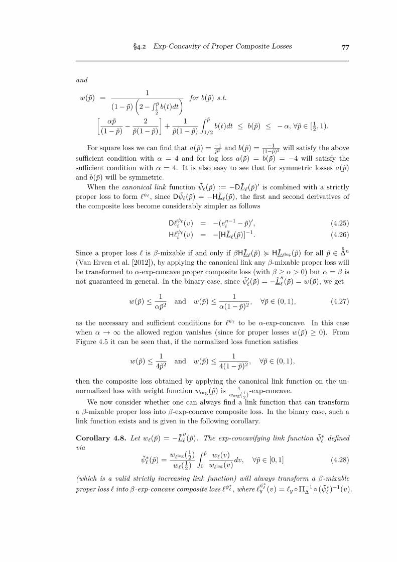
§4.2 Exp-Concavity of Proper Composite Losses 77
and
w(p) =
1
(1 ≠ p)3
2 ≠ s p12
b(t)dt4 for b(p) s.t.
5
–p
(1 ≠ p)≠ 2
p(1 ≠ p)
6
+
1p(1 ≠ p)
⁄ p
1/2b(t)dt Æ b(p) Æ ≠ –, ’p œ [
12 , 1).
For square loss we can find that a(p) = ≠1p2 and b(p) = ≠1
(1≠p)2 will satisfy the abovesu�cient condition with – = 4 and for log loss a(p) = b(p) = ≠4 will satisfy thesu�cient condition with – = 4. It is also easy to see that for symmetric losses a(p)and b(p) will be symmetric.
When the canonical link function ¸(p) := ≠DL¸(p)Õ is combined with a strictly
proper loss to form ¸Â¸ , since D¸(p) = ≠HL¸(p), the first and second derivatives ofthe composite loss become considerably simpler as follows
D¸Â¸i (v) = ≠(en≠1
i ≠ p)Õ, (4.25)H¸Â¸
i (v) = ≠[HL¸(p)]≠1. (4.26)
Since a proper loss ¸ is —-mixable if and only if —HL¸(p) < HL¸log(p) for all p œ ˚Dn
(Van Erven et al. [2012]), by applying the canonical link any —-mixable proper loss willbe transformed to –-exp-concave proper composite loss (with — Ø – > 0) but – = — isnot guaranteed in general. In the binary case, since ÂÕ
¸(p) = ≠LÕÕ¸ (p) = w(p), we get
w(p) Æ 1–p2 and w(p) Æ 1
–(1 ≠ p)2 , ’p œ (0, 1), (4.27)
as the necessary and su�cient conditions for ¸Â¸ to be –-exp-concave. In this casewhen – æ Œ the allowed region vanishes (since for proper losses w(p) Ø 0). FromFigure 4.5 it can be seen that, if the normalized loss function satisfies
w(p) Æ 14p2 and w(p) Æ 1
4(1 ≠ p)2 , ’p œ (0, 1),
then the composite loss obtained by applying the canonical link function on the un-normalized loss with weight function worg(p) is 4
worg(12 )
-exp-concave.We now consider whether one can always find a link function that can transform
a —-mixable proper loss into —-exp-concave composite loss. In the binary case, such alink function exists and is given in the following corollary.
Corollary 4.8. Let w¸(p) = ≠LÕÕ¸ (p). The exp-concavifying link function Âú
¸ definedvia
Âú¸ (p) =
w¸log(12 )
w¸(12 )
⁄ p
0
w¸(v)
w¸log(v)dv, ’p œ [0, 1] (4.28)
(which is a valid strictly increasing link function) will always transform a —-mixableproper loss ¸ into —-exp-concave composite loss ¸Âú
¸ , where ¸Âú
¸y (v) = ¸y ¶ P≠1
D ¶ (Âú¸ )
≠1(v).

78 Exp-concavity of Proper Composite Losses
For log loss, the exp-concavifying link is equal to the identity link and the canonicallink could be written as
s p0 w¸(v)dv. If ¸ is a binary proper loss with weight function
w¸(p), then we can define a new proper loss ¸mix with weight function w¸mix(p) =
w¸(p)w
¸log (p). Then applying the exp-concavifying link Âú
¸ on the original loss ¸ is equivalentto applying the canonical link ¸ on the new loss ¸mix.
The links constructed by the geometric and calculus approaches can be completelydi�erent (see Appendix 4.4.4, 4.4.5, and 4.4.6). The former can be further varied byreplacing 1n with any direction in the positive orthant, and the latter can be arbitrar-ily rescaled. Furthermore, as both links satisfy (4.21) with – = —, any appropriateinterpolation also works.
4.3 Conclusions
If a loss is —-mixable, one can run the Aggregating Algorithm with learning rate —and obtain a log N
— regret bound. Similarly a log N– regret bound can be attained by
the Weighted Average Algorithm with learning rate –, when the loss is –-exp-concave.Vovk [2001] observed that the weighted average of the expert predictions (Kivinenand Warmuth [1999]) will be a perfect (in the technical sense defined in Vovk [2001])substitution function for the Aggregating Algorithm if and only if the loss functionis exp-concave. Thus if we have to use a proper, mixable but non-exp-concave lossfunction ¸ for a sequential prediction (online learning) problem, an O(1) regret boundcould be achieved by the following two approaches:
• Use the Aggregating Algorithm (Vovk [1995]) with the inverse loss ¸≠1 (Williamson[2014]) as the universal substitution function.
• Apply the exp-concavifying link (Âú¸ ) on ¸, derive the —¸-exp-concave compos-
ite loss ¸Âú¸ . Then use the Weighted Average Algorithm (Kivinen and War-
muth [1999]) with ¸Âú¸ to obtain the learner’s prediction in the transformed do-
main (vavg œ Âú¸ (D
n)). Finally output the inverse link value of this prediction
((Âú¸ )
≠1(vavg)).
In either approach we are faced with a computational problem of evaluating an inversefunction. But in the binary class case the inverse of a strictly monotone functioncan be e�ciently evaluated using one sided bisection method (or lookup table). So inconclusion, the latter approach can be more convenient and e�cient in computationthan the former.
When n = 2, we have shown that one can always transform a beta-mixable properloss into beta-exp-concave proper composite loss using either geometric link function(Proposition 4.1) or calculus-based link function (Corollary 4.8). When n > 2, weobserved that the square loss (which is a mixable proper loss) cannot be exp-concavifiedvia the geometric link. And by the calculus approach, it is hard to obtain an explicitform for exp-concavifying link function when n > 2. Thus when n > 2, characterizationof proper mixable losses that are exp-concavifiable still remains an open problem. For

§4.4 Appendix 79
`�1
(v)
`+1
(v)
(`�1
(v1
), `1
(v1
))
(`�1
(v2
), `1
(v2
))
(`�1
(vinv
), `1
(vinv
))
(g(�1), g(1))
S`
Figure 4.6: Super-prediction set (S¸) of a binary game ({≠1, 1}, [0, 1], ¸), where ageneralized prediction is represented by (g(≠1), g(1)).
this, we may need to consider other possible ways to construct link functions Williamson[2014].
4.4 Appendix
4.4.1 Substitution Functions
We consider the following choices of substitution functions — Best look ahead, Worstlook ahead, Inverse loss (Williamson [2014]) and Weighted average (Kivinen and War-muth [1999]). The first two choices are just hypothetical ones as they look ahead theactual outcome first and then choose their predictions to incur low and high loss re-spectively, still they give us an idea about how well or worse the Aggregating Algorithmperforms over a given outcome sequence. The weighted average is a computationallye�cient and easily implementable substitution function, but it is applicable only forexp-concave losses.
For a binary game represented by(
{≠1, 1}, [0, 1], ¸)
and shown in the Figure 4.6,
• If the outcome y = ≠1, the Best look ahead and the Worst look ahead willchoose the predictions v2 and v1 and incur losses ¸≠1(v2) and ¸≠1(v1) = g(≠1)respectively; and if y = 1, they will choose v1 and v2 and su�er losses ¸1(v1) and¸1(v2) = g(1) respectively.
• The Inverse loss will choose the prediction vinv such that ¸1(vinv)¸≠1(vinv)
=
g(1)g(≠1) and will
incur a loss ¸(y, vinv), and the Weighted average will choose vavg =
q
i wivi (wherewi and vi are the weight and the prediction of the i-the expert respectively) andwill incur a loss ¸(y, vavg).
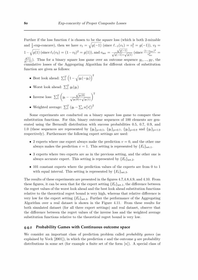
80 Exp-concavity of Proper Composite Losses
Further if the loss function ¸ is chosen to be the square loss (which is both 2-mixableand 1
2 -exp-concave), then we have v1 =
Ò
g(≠1) (since ¸≠1(v1) = v21 = g(≠1)), v2 =
1≠Ò
g(1) (since ¸1(v2) = (1≠v2)2= g(1)), and vinv =
Ôg(≠1)Ô
g(≠1)+Ô
g(1)(since (1≠vinv)2
v2inv
=
g(1)g(≠1) ). Thus for a binary square loss game over an outcome sequence y1, ..., yT , thecumulative losses of the Aggregating Algorithm for di�erent choices of substitutionfunction are given as follows:
• Best look ahead:qT
11
1 ≠Ò
gt(≠yt)
22
• Worst look ahead:qT
1 gt(yt)
• Inverse loss:qT
1
3
yt ≠Ô
gt(0)Ôgt(0)+
Ôgt(1)
42
• Weighted average:qT
1 (
yt ≠ q
i wtiv
ti)
2
Some experiments are conducted on a binary square loss game to compare thesesubstitution functions. For this, binary outcome sequences of 100 elements are gen-erated using the Bernoulli distribution with success probabilities 0.5, 0.7, 0.9, and1.0 (these sequences are represented by {yt}p=0.5, {yt}p=0.7, {yt}p=0.9 and {yt}p=1.0respectively). Furthermore the following expert settings are used:
• 2 experts where one expert always make the prediction v = 0, and the other onealways makes the prediction v = 1. This setting is represented by {Et}set.1.
• 3 experts where two experts are as in the previous setting, and the other one isalways accurate expert. This setting is represented by {Et}set.2.
• 101 constant experts where the prediction values of the experts are from 0 to 1with equal interval. This setting is represented by {Et}set.3.
The results of these experiments are presented in the figures 4.7,4.8,4.9, and 4.10. Fromthese figures, it can be seen that for the expert setting {Et}set.1, the di�erence betweenthe regret values of the worst look ahead and the best look ahead substitution functionsrelative to the theoretical regret bound is very high, whereas that relative di�erence isvery low for the expert setting {Et}set.3. Further the performance of the AggregatingAlgorithm over a real dataset is shown in the Figure 4.11. From these results forboth simulated dataset (for all three expert settings) and real dataset, observe thatthe di�erence between the regret values of the inverse loss and the weighted averagesubstitution functions relative to the theoretical regret bound is very low.
4.4.2 Probability Games with Continuous outcome space
We consider an important class of prediction problem called probability games (asexplained by Vovk [2001]), in which the prediction v and the outcome y are probabilitydistributions in some set (for example a finite set of the form [n]). A special class of
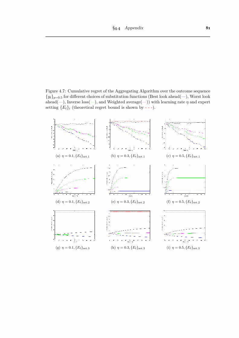
§4.4 Appendix 81
Figure 4.7: Cumulative regret of the Aggregating Algorithm over the outcome sequence{yt}p=0.5 for di�erent choices of substitution functions (Best look ahead(—), Worst lookahead(—), Inverse loss(—), and Weighted average(—)) with learning rate ÷ and expertsetting {Et}i (theoretical regret bound is shown by - - -).
(a) ÷ = 0.1, {Et}set.1 (b) ÷ = 0.3, {Et}set.1 (c) ÷ = 0.5, {Et}set.1
(d) ÷ = 0.1, {Et}set.2 (e) ÷ = 0.3, {Et}set.2 (f) ÷ = 0.5, {Et}set.2
(g) ÷ = 0.1, {Et}set.3 (h) ÷ = 0.3, {Et}set.3 (i) ÷ = 0.5, {Et}set.3

82 Exp-concavity of Proper Composite Losses
Figure 4.8: Cumulative regret of the Aggregating Algorithm over the outcome sequence{yt}p=0.7 for di�erent choices of substitution functions (Best look ahead(—), Worst lookahead(—), Inverse loss(—), and Weighted average(—)) with learning rate ÷ and expertsetting {Et}i (theoretical regret bound is shown by - - -).
(a) ÷ = 0.1, {Et}set.1 (b) ÷ = 0.3, {Et}set.1 (c) ÷ = 0.5, {Et}set.1
(d) ÷ = 0.1, {Et}set.2 (e) ÷ = 0.3, {Et}set.2 (f) ÷ = 0.5, {Et}set.2
(g) ÷ = 0.1, {Et}set.3 (h) ÷ = 0.3, {Et}set.3 (i) ÷ = 0.5, {Et}set.3

§4.4 Appendix 83
Figure 4.9: Cumulative regret of the Aggregating Algorithm over the outcome sequence{yt}p=0.9 for di�erent choices of substitution functions (Best look ahead(—), Worst lookahead(—), Inverse loss(—), and Weighted average(—)) with learning rate ÷ and expertsetting {Et}i (theoretical regret bound is shown by - - -).
(a) ÷ = 0.1, {Et}set.1 (b) ÷ = 0.3, {Et}set.1 (c) ÷ = 0.5, {Et}set.1
(d) ÷ = 0.1, {Et}set.2 (e) ÷ = 0.3, {Et}set.2 (f) ÷ = 0.5, {Et}set.2
(g) ÷ = 0.1, {Et}set.3 (h) ÷ = 0.3, {Et}set.3 (i) ÷ = 0.5, {Et}set.3

84 Exp-concavity of Proper Composite Losses
Figure 4.10: Cumulative regret of the Aggregating Algorithm over the outcome se-quence {yt}p=1.0 for di�erent choices of substitution functions (Best look ahead(—),Worst look ahead(—), Inverse loss(—), and Weighted average(—)) with learning rate÷ and expert setting {Et}i (theoretical regret bound is shown by - - -).
(a) ÷ = 0.1, {Et}set.1 (b) ÷ = 0.3, {Et}set.1 (c) ÷ = 0.5, {Et}set.1
(d) ÷ = 0.1, {Et}set.2 (e) ÷ = 0.3, {Et}set.2 (f) ÷ = 0.5, {Et}set.2
(g) ÷ = 0.1, {Et}set.3 (h) ÷ = 0.3, {Et}set.3 (i) ÷ = 0.5, {Et}set.3
Figure 4.11: Cumulative regret of the Aggregating Algorithm over the football datasetas used by Vovk and Zhdanov [2009], for di�erent choices of substitution functions (Bestlook ahead(—), Worst look ahead(—), Inverse loss(—), and Weighted average(—)) withlearning rate ÷ (theoretical regret bound is shown by - - -).
(a) ÷ = 0.1 (b) ÷ = 0.3 (c) ÷ = 0.5

§4.4 Appendix 85
loss functions called Bregman Loss Functions (defined below) would be an appropriatechoice for the probability games.
Given a di�erentiable convex function „ : S æ R defined on a convex set S µ Rd
and two points s0, s œ S the Bregman divergence of s from s0 is defined as
B„(s, s0) := „(s) ≠ „(s0) ≠ (s ≠ s0)Õ · D„(s0),
where D„(s0) is the gradient of „ at s0. For any strictly convex function „ : Dn æ R,di�erentiable over the interior of Dn, the Bregman Loss Function (BLF, Banerjee et al.[2005]) ¸„ : Dn ◊ Dn æ R
+
with generator „ is given by
¸„(y, v) := B„(y, v) = „(y) ≠ „(v) ≠ (y ≠ v)Õ · D„(v); y, v œ Dn, (4.29)
where y = PD(y), and v = PD(v). Since the conditional Bayes risk of a strictlyproper loss is strictly concave, any di�erentiable strictly proper loss ¸ : Dn æ Rn
+
willgenerate a BLF ¸„ with generator „ = ≠L¸. Further if ¸ is fair, ¸i(v) = ¸„(en
i , v); i.e.reconstruction is possible. For example the Kullback-Leibler loss given by ¸KL(y, v) :=qn
i=1 y(i) log y(i)v(i) , is a BLF generated by the log loss which is strictly proper.
The following lemma (multi-class extension of a result given by Haussler et al.[1998]) provides the mixability condition for probability games.
Lemma 4.9. For given ¸ : Dn ◊ Dn æ R+
, assume that for all y, v1, v2 œ Dn (lety = P≠1
D (y), v1 = P≠1D (v1), and v2 = P≠1
D (v2)), the function g defined by
g(y, v1, v2) =—
c(—)¸(y, v1) ≠ —¸(y, v2) (4.30)
satisfiesHyg(y, v1, v2) + Dyg(y, v1, v2) · (Dyg(y, v1, v2))
Õ < 0. (4.31)
If÷vú œ Dn s.t. ¸(y, vú
) Æ ≠c(—)
—log
⁄
e≠—¸(y,v)P (dv) (4.32)
holds for the vertices y = en≠1i , i œ [n], then it holds for all values y œ Dn (where
y = P≠1D (y), vú
= P≠1D (vú
) and v = P≠1D (v)).
Proof. From (4.32)
—
c(—)¸(y, vú
) + log⁄
e≠—¸(y,v)P (dv) Æ 0.
By exponentiating both sides we get
e—
c(—)
¸(y,vú) ·
⁄
e≠—¸(y,v)P (dv) Æ 1.

86 Exp-concavity of Proper Composite Losses
Denoting the left hand side of the above inequality by f(y) we have
f(y) =⁄
eg(y,vú,v)P (dv).
Since the Hessian of f w.r.t. y given by
Hyf(y) =⁄
eg(y,vú,v)(
Hyg(y, vú, v) + Dyg(y, vú, v) · (Dyg(y, vú, v))Õ)
P (dv)
is positive semi-definite (by (4.31)), f(y) is convex in y. So the maximum values of ffor y œ Dn occurs for some y = en≠1
i , i œ [n]. And by noting that, (4.32) is equivalentto f(y) Æ 1 for y = en≠1
i , i œ [n], the proof is completed.
The next proposition shows that the mixability and exp-concavity of a strictlyproper loss is carried over to the BLF generated by it.
Proposition 4.10. For a strictly proper fair loss ¸ : Dn æ Rn+
, and the BLF ¸„ :Dn ◊ Dn æ R
+
generated by ¸ with „ = ≠L¸ , if ¸ is —-mixable (resp. –-exp-concave),then ¸„ is also —-mixable (resp. –-exp-concave).
Proof. From (4.30) and (4.29), for the BLF ¸„ we have
g(y, v1, v2) =—
c(—){„(y) ≠ „(v1) ≠ (y ≠ v1)
Õ · D„(v1)}
≠ —{„(y) ≠ „(v2) ≠ (y ≠ v2)Õ · D„(v2)},
Dyg(y, v1, v2) =—
c(—){D„(y) ≠ D„(v1)} ≠ —{D„(y) ≠ D„(v2)},
Hyg(y, v1, v2) =—
c(—)H„(y) ≠ —H„(y).
And since x · xÕ < 0, ’x œ Rn, (4.31) is satisfied for all y, v1, v2 œ Dn when c(—) = 1,which is the mixability condition (in addition requiring vú
=
s
vP (dv) in (4.32) is theexp-concavity condition). Then by applying Lemma 4.9 proof is completed.
As an application of Proposition 4.10, we can see that both Kullback-Leibler lossand log loss are 1-mixable and 1-exp-concave.
4.4.3 Proofs
Proof. (Proposition 4.1) We first prove that the set Â(Dn) is convex. For any p, q œ
Dn, by assumption there exists c Ø 0 and r œ Dn such that 12 (E—(¸(p)) + E—(¸(q))) +
c1n = E—(¸(r)). Therefore 12 (Â(p) +Â(q)) = Â(r), which implies the convexity of the
set Â(Dn).
Let T : Rn≠1 – (e≠—z1 ≠ e≠—zn , ..., e≠—zn≠1 ≠ e≠—zn)
Õ æ (e≠—z1 , ..., e≠—zn)
Õ œ [0, 1]n.Note this mapping from low dimension to high dimension is well defined because ifthere are two di�erent z and z in ¸(V) such that JE—(z) = JE—(z), then there must

§4.4 Appendix 87
be c ”= 0 such that E—(z) + c1 = E—(z). This means z > z or z < z, which violatesthe strict properness of ¸.
Since for any v = Â(p) = JE—(¸(p)) we have p = ¸≠11
E≠1— (Tv)
2
, the link  isinvertible (¸ is invertible if it is strictly proper (Williamson et al. [2016]), and E— isinvertible for — > 0).
Now ¸ ¶ Â≠1 is —-exp-concave if for all p, q œ Dn
E—
3
¸ ¶ Â≠131
2 (Â(p) + Â(q))44
Ø 12E—
1
¸ ¶ Â≠1(Â(p))
2
+
12E—
1
¸ ¶ Â≠1(Â(q))
2
.(4.33)
The right-hand side is obviously 12 (E—(¸(p)) + E—(¸(q))). Let r = Â≠1
1
12 (Â(p) + Â(q))
2
œDn. Then
JE—(¸(r)) = Â(r) =12 (
JE—(¸(p)) + JE—(¸(q))) .
Therefore 12 (E—(¸(p)) + E—(¸(q))) = E—(¸(r)) + c1n for some c œ R. To establish
(4.33), it su�ces to show c Æ 0. But this is guaranteed by the condition assumed.
Proof. (Proposition 4.2) We first show that for a half space H“p≠p defined in (4.11)
with p œ Dn‘ , E≠1
— (H“p≠p fl Rn
+
) must be the super-prediction set of a scaled and shiftedlog loss. In fact, as pi > 0, clearly “p = minxœT¸ xÕ · (≠p) < 0. Define a new loss˜logi (q) = ≠ 1
— log(≠“p
piqi) over q œ Dn. Then S ˜log ™ E≠1
— (H“p≠p fl Rn
+
) can be seen from
ÿ
i
(≠pi) exp(≠— ˜logi (q)) =
ÿ
i
(≠pi)(≠“p
piqi) = “p. (4.34)
Conversely, for any u such that ui > 0 and (≠p)Õ · u = “p, simply choose qi = ≠uipi“p
.Then q œ Dn and E—(
˜log(q)) = u. In summary, E≠1
— (H“p≠p fl Rn
+
) is the super-predictionset of ˜log.
To prove Proposition 4.2, we first show that for any point a œ T ‘¸ and any direction
d from the relative interior of the positive orthant (which includes the 1n direction),the ray {a + rd : r Ø 0} will be blocked by a boundary point of T ‘
¸ . This is becauseby the definition of T ‘
¸ in (4.12), the largest value of r to guarantee a+ rd œ T ‘¸ can be
computed by
rú := sup{r Ø 0 : a + rd œ T ‘¸ } = sup{r Ø 0 : (a + rd)Õ · (≠p) Ø “p, ’p œ Dn
‘ } (4.35)
must be finite and attained. Denote x = a + rúd, which must be on the boundary ofT ‘
¸ because
≠xÕ · p Ø “p, for all p œ Dn‘ , (4.36)
and ≠ xÕ · pú= “pú for some pú œ Dn
‘ (not necessarily unique). (4.37)
In order to prove the first statement of Proposition 4.2, it su�ces to show that for anypoint x on the north-east boundary of T ‘
¸ , there exists a q œ Dn such that E—(˜‘(q)) = x.
Suppose x satisfies (4.36) and (4.37). Then consider the (shifted/scaled) log loss ˜log
that corresponds to H“púpú . Because log loss is strictly proper, there must be a unique

88 Exp-concavity of Proper Composite Losses
q œ Dn such that the hyperplane H0 := {z : qÕ · z = qÕ · E≠1— (x)} supports the super-
prediction set of ˜log (i.e., E≠1— (H
“pú≠pú fl Rn
+
)) at E≠1— (x). Since E≠1
— (T ‘¸ fl Rn
+
) is aconvex subset of E≠1
— (H“pú≠pú fl Rn
+
), this hyperplane also supports E≠1— (T ‘
¸ fl Rn+
) atE≠1
— (x). Therefore E≠1— (x) is an optimal solution to the problem in the definition of
˜‘(q) in (4.13). Finally observe that it must be the unique optimal solution, because ifthere were another solution which also lies on H0, then by the convexity of the super-prediction set of ˜‘, the line segment between them must also lie on the predictionset of ˜‘. This violates the mixability condition of ˜‘, because by construction itssub-exp-prediction set is convex.
In order to check where ¸(p) =
˜‘(p), a su�cient condition is that the normaldirection d on the exp-prediction set evaluated at E—(¸(p)) satisfies di/
q
j dj > ‘.Simple calculus shows that di à pi exp(—¸i(p)). Therefore as long as p is in the relativeinterior of Dn, di/
q
j dj > ‘ can always be satisfied by choosing a su�ciently small ‘.And for each fixed ‘, the set S‘ mentioned in the theorem consists exactly of all suchp that satisfies this condition.
Proof. (Proposition 4.5) When n = 2, (4.17), (4.18) and (4.19) and the positivity ofÂÕ simplify (4.20) to the two conditions:
(1 ≠ p) kÕ(p) Æ k(p) ≠ – ÂÕ
(p) k(p)2(1 ≠ p)2,
≠p kÕ(p) Æ k(p) ≠ – ÂÕ
(p) k(p)2 p2,
for all p œ (0, 1). These two conditions can be merged as follows
≠1p+ – ÂÕ
(p) k(p) p Æ kÕ(p)
k(p)Æ 1
1 ≠ p≠ – ÂÕ
(p) k(p) (1 ≠ p), ’p œ (0, 1).
By noting that k(p) = w(p)ÂÕ
(p)and kÕ
(p) = wÕ(p)ÂÕ
(p)≠w(p)ÂÕÕ(p)
ÂÕ(p)
2 completes the proof.
Proof. (Proposition 4.6) Let g(p) =
1w(p) and so gÕ
(p) = ≠ 1w(p)2 wÕ
(p), g(v) =
s v12
gÕ(p)dp + g( 1
2 ) and g( 12 ) =
1w(
12 )
= 1. By dividing all sides of (4.21) by ≠w(p)
and applying the substitution we get,
1p
g(p) ≠ –p Ø gÕ(p) ≠ FÂ(p)g(p) Ø ≠ 1
1 ≠ pg(p) + –(1 ≠ p), ’p œ (0, 1), (4.38)
where FÂ(p) := ≠ ÂÕÕ(p)
ÂÕ(p)
. If we take the first inequality of (4.38) and rearrange it weobtain,
≠ – Ø3
gÕ(p)
1p
≠ g(p)1p2
4
≠ FÂ(p)g(p)
p=
3
g(p)
p
4Õ≠ FÂ(p)
3
g(p)
p
4
, ’p œ (0, 1).(4.39)

§4.4 Appendix 89
Multiplying (4.39) by e≠s p
0 FÂ(t)dt will result in,
≠–e≠s p
0 FÂ(t)dt Ø3
g(p)
p
4Õe≠
s p
0 FÂ(t)dt+
3
g(p)
p
4
e≠s p
0 FÂ(t)dt(≠FÂ(p))
=
3
g(p)
pe≠
s p
0 FÂ(t)dt4Õ
, ’p œ (0, 1). (4.40)
Since≠
⁄ p
0FÂ(t)dt = ≠
⁄ p
0≠ ÂÕÕ
(t)
ÂÕ(t)
dt =⁄ p
0(log ÂÕ
(t))Õdt = log ÂÕ(p)
ÂÕ(0)
,
(4.40) is reduced to
≠–ÂÕ(p)
ÂÕ(0)
ØA
g(p)
p
ÂÕ(p)
ÂÕ(0)
BÕ, ’p œ (0, 1)
∆ ≠–ÂÕ(p) Ø
3
g(p)
pÂÕ(p)
4Õ, ’p œ (0, 1).
For v Ø 12 we thus have
≠–⁄ v
12
ÂÕ(p)dp Ø
⁄ v
12
3
g(p)
pÂÕ(p)
4Õdp, ’v œ [1/2, 1)
∆ ≠–(Â(v) ≠ Â(12 )) Ø
A
g(v)
vÂÕ(v) ≠ g( 1
2 )12
ÂÕ(
12 )
B
=
3 1w(v)v
ÂÕ(v) ≠ 2ÂÕ
(
12 )
4
, ’v œ [1/2, 1)
∆ w(v) Ø ÂÕ(v)
v(2ÂÕ(
12 ) ≠ –(Â(v) ≠ Â( 1
2 ))), ’v œ [1/2, 1).
Also by considering v Æ 12 case as above, we get
ÂÕ(v)
v(2ÂÕ(
12 ) ≠ –(Â(v) ≠ Â( 1
2 )))Q w(v), ’v œ (0, 1).
Finally by following the similar steps for the second inequality of (4.38), the proof willbe completed.
Here we provide an integral inequalities related result (without proof) due to Bee-sack and presented in Dragomir [2000].
Theorem 4.11. Let y and k be continuous and f and g Riemann integrable functionson J = [–, —] with g and k nonnegative on J . If
y(x) Ø f(x) + g(x)⁄ x
–y(t)k(t)dt, x œ J ,

90 Exp-concavity of Proper Composite Losses
theny(x) Ø f(x) + g(x)
⁄ x
–f(t)k(t) exp
3
⁄ x
tg(r)k(r)dr
4
dt, x œ J .
The result remains valid ifs x
– is replaced bys —
x ands x
t bys t
x throughout.
Using the above theorem, we get the following simplified test for the conditions inTheorem 4.7:
≠–+
–
2p2 ≠ 2p2 Æ a(p) =∆
5
–(1 ≠ p)
p≠ 2
p(1 ≠ p)
6
+
1p(1 ≠ p)
⁄ 1/2
pa(t)dt Æ a(p)
and
–p
(1 ≠ p)+
2–p≠–≠42(1 ≠ p)2 Æ b(p) =∆
5
–p
(1 ≠ p)≠ 2
p(1 ≠ p)
6
+
1p(1 ≠ p)
⁄ p
1/2b(t)dt Æ b(p).
Above two identities are proved in the following proof of Theorem 4.7.
Proof. (Theorem 4.7) The necessary and su�cient condition for the exp-concavityof proper losses is given by (4.23). But from (4.39), we can see that (4.23) is equivalentto
3
g(p)
p
4ÕÆ ≠–, ’p œ (0, 1), (4.41)
and≠
3
g(p)
1 ≠ p
4ÕÆ ≠–, ’p œ (0, 1), (4.42)
where g(p) = 1w(p) with w(
12 ) = 1; i.e. (4.23) if and only if (4.41) & (4.42).
Now if we choose the weight function w(p) as follows
w(p) =1
p1
2 +s p
1/2 a(t)dt2 , (4.43)
such that a(t) Æ ≠–, then (4.41) will be satisfied (since (4.43) =∆ 2 +s p
1/2 a(t)dt =1
w(p)p =
g(p)p =∆ a(p) =
1
g(p)p
2Õ). Similarly the weight function w(p) given by
w(p) =1
(1 ≠ p)1
2 ≠ s p1/2 b(t)dt
2 , (4.44)
with b(t) Æ ≠– will satisfy (4.42) (since (4.44) =∆ 2 ≠ s p1/2 b(t)dt =
1w(p)(1≠p) =
g(p)1≠p =∆ ≠b(p) =
1
g(p)1≠p
2Õ). To satisfy both (4.41) and (4.42) at the same time (then
obviously (4.23) will be satisfied), we can make the two forms of the weight function((4.43) and (4.44)) equivalent with the appropriate choice of a(t) and b(t). This canbe done in two cases.
In the first case, for p œ (0, 1/2] we can fix the weight function w(p) as given by(4.43) and choose a(t) such that,
§4.4 Appendix 91
• a(t) Æ ≠– (then (4.41) is satisfied) and
• (4.43) = (4.44) =∆ b(t) Æ ≠– (then (4.42) is satisfied).
But (4.43) = (4.44) for all p œ (0, 1/2] if and only if
p
A
2 ≠⁄ 1/2
pa(t)dt
B
= (1 ≠ p)
A
2 +⁄ 1/2
pb(t)dt
B
, p œ (0, 1/2]
≈∆ p
1 ≠ p
A
2 ≠⁄ 1/2
pa(t)dt
B
≠ 2 =
⁄ 1/2
pb(t)dt, p œ (0, 1/2]
≈∆ p
1 ≠ pa(p) +
1(1 ≠ p)2
A
2 ≠⁄ 1/2
pa(t)dt
B
= ≠b(p), p œ (0, 1/2],
where the last step is obtained by di�erentiating both sides w.r.t p. Thus the constraint(4.43) = (4.44) =∆ b(t) Æ ≠– can be given as
p
1 ≠ pa(p) +
1(1 ≠ p)2
A
2 ≠⁄ 1/2
pa(t)dt
B
Ø –, p œ (0, 1/2]
≈∆ a(p) Ø5
–(1 ≠ p)
p≠ 2
p(1 ≠ p)
6
+
1p(1 ≠ p)
⁄ 1/2
pa(t)dt, p œ (0, 1/2]
≈∆ a(p) Ø f(p) + g(p)⁄ 1/2
pa(t)k(t)dt, p œ (0, 1/2],
where f(p) =
Ë
–(1≠p)p ≠ 2
p(1≠p)
È
, g(p) =
1p(1≠p) =
1p +
1(1≠p) and k(t) = 1. Now by
applying Theorem 4.11 we have
a(p) Ø f(p) + g(p)⁄ 1/2
pf(t)k(t) exp
3
⁄ t
pg(r)k(r)dr
4
dt, p œ (0, 1/2].
Since⁄ t
pg(r)k(r)dr =
⁄ t
p
1r+
1(1 ≠ r)
dr = [ln r ≠ ln(1 ≠ r)]tp = ln3
t
(1 ≠ t)
(1 ≠ p)
p
4
,
⁄ 1/2
pf(t)k(t) exp
3
⁄ t
pg(r)k(r)dr
4
dt =
⁄ 1/2
pf(t)
t
(1 ≠ t)
(1 ≠ p)
pdt
=
(1 ≠ p)
p
⁄ 1/2
p
5
–(1 ≠ t)
t≠ 2
t(1 ≠ t)
6
t
(1 ≠ t)dt
=
(1 ≠ p)
p
⁄ 1/2
p– ≠ 2
(1 ≠ t)2 dt
=
(1 ≠ p)
p
5
–t ≠ 21 ≠ t
61/2
p
=
(1 ≠ p)
p
5
–
2 ≠ 4 ≠ –p +2
1 ≠ p
6
,

92 Exp-concavity of Proper Composite Losses
we get
a(p) Ø5
–(1 ≠ p)
p≠ 2
p(1 ≠ p)
6
+
1p(1 ≠ p)
(1 ≠ p)
p
5
–
2 ≠ 4 ≠ –p +2
1 ≠ p
6
, p œ (0, 1/2]
= ≠– +
–
2p2 ≠ 2p2 , p œ (0, 1/2].
Similarly in the second case, for p œ [1/2, 1) we can fix the weight function w(p)as given by (4.44) and choose b(t) such that,
• b(t) Æ ≠– (then (4.42) is satisfied) and
• (4.43) = (4.44) =∆ a(t) Æ ≠– (then (4.41) is satisfied).
But (4.43) = (4.44) for all p œ [1/2, 1) if and only if
p3
2 +⁄ p
1/2a(t)dt
4
= (1 ≠ p)3
2 ≠⁄ p
1/2b(t)dt
4
, p œ [1/2, 1)
≈∆⁄ 1/2
pa(t)dt =
1 ≠ p
p
3
2 ≠⁄ p
1/2b(t)dt
4
≠ 2, p œ [1/2, 1)
≈∆ a(p) = ≠1 ≠ p
pb(p) ≠ 1
p2
3
2 ≠⁄ p
1/2b(t)dt
4
, p œ [1/2, 1),
where the last step is obtained by di�erentiating both sides w.r.t p. Thus the constraint(4.43) = (4.44) =∆ a(t) Æ ≠– can be given as
1 ≠ p
pb(p) +
1p2
3
2 ≠⁄ p
1/2b(t)dt
4
Ø –, p œ [1/2, 1)
≈∆ b(p) Ø5
–p
(1 ≠ p)≠ 2
p(1 ≠ p)
6
+
1p(1 ≠ p)
⁄ p
1/2b(t)dt, p œ [1/2, 1)
≈∆ b(p) Ø f(p) + g(p)⁄ p
1/2b(t)k(t)dt, p œ [1/2, 1),
where f(p) =
Ë
–p(1≠p) ≠ 2
p(1≠p)
È
, g(p) =
1p(1≠p) =
1p +
1(1≠p) and k(t) = 1. Again by
applying Theorem 4.11 we have
b(p) Ø f(p) + g(p)⁄ p
1/2f(t)k(t) exp
3
⁄ p
tg(r)k(r)dr
4
dt, p œ [1/2, 1).
Since⁄ p
tg(r)k(r)dr =
⁄ p
t
1r+
1(1 ≠ r)
dr = [ln r ≠ ln(1 ≠ r)]pt = ln3
p
(1 ≠ p)
(1 ≠ t)
t
4
,
⁄ p
1/2f(t)k(t) exp
3
⁄ p
tg(r)k(r)dr
4
dt =
⁄ p
1/2f(t)
p
(1 ≠ p)
(1 ≠ t)
tdt
=
p
(1 ≠ p)
⁄ p
1/2
5
–t
(1 ≠ t)≠ 2
t(1 ≠ t)
6
(1 ≠ t)
tdt

§4.4 Appendix 93
=
p
(1 ≠ p)
⁄ p
1/2– ≠ 2
t2 dt
=
p
(1 ≠ p)
5
–t +2t
6p
1/2
=
p
(1 ≠ p)
5
–p +2p
≠ –
2 ≠ 46
,
we get
b(p) Ø5
–p
(1 ≠ p)≠ 2
p(1 ≠ p)
6
+
1p(1 ≠ p)
p
(1 ≠ p)
5
–p +2p
≠ –
2 ≠ 46
, p œ [1/2, 1)
=
–p
(1 ≠ p)+
–p
(1 ≠ p)2 ≠ –
2(1 ≠ p)2 ≠ 2(1 ≠ p)2 , p œ [1/2, 1).
Proof. (Corollary 4.8) We have to show that Âú¸ will satisfy (4.21) with – = —, for
all —-mixable proper loss functions. Since
(Âú¸ )
ÕÕ(p)
(Âú¸ )
Õ(p)
=
wÕ¸(p)w¸log (p)≠w¸(p)wÕ
¸log (p)
w¸log (p)
2
w¸(p)w
¸log (p)
=
wÕ¸(p)
w¸(p)≠ wÕ
¸log(p)
w¸log(p)=
wÕ¸(p)
w¸(p)≠ (log w¸log(p))Õ,
(4.45)by substituting  = Âú
¸ and – = — in (4.21) we have,
≠1p+ —w¸(p)p Æ wÕ
¸(p)
w¸(p)≠ (Âú
¸ )ÕÕ(p)
(Âú¸ )
Õ(p)
Æ 11 ≠ p
≠ —w¸(p)(1 ≠ p), ’p œ (0, 1)
≈∆ ≠1p+ —w¸(p)p Æ (log w¸log(p))Õ Æ 1
1 ≠ p≠ —w¸(p)(1 ≠ p), ’p œ (0, 1)
≈∆ ≠1p+ —w¸(p)p Æ ≠1
p+
11 ≠ p
Æ 11 ≠ p
≠ —w¸(p)(1 ≠ p), ’p œ (0, 1)
≈∆ — Æ 1p(1 ≠ p)w¸(p)
=
w¸log(p)
w¸(p), ’p œ (0, 1),
which is true for all —-mixable binary proper loss functions. From (4.45)
1
log (Âú¸ )
Õ(p)
2Õ= (log w¸(p))
Õ ≠ (log w¸log(p))Õ=
3
log w¸(p)
w¸log(p)
4Õ,
∆Ë
log (Âú¸ )
Õ(p)
Èp
1/2=
5
log w¸(p)
w¸log(p)
6p
1/2,
∆ log (Âú¸ )
Õ(p) ≠ log (Âú
¸ )Õ31
2
4
= log w¸(p)
w¸log(p)· w¸log(
12 )
w¸(12 )
,
it can be seen that a design choice of (Âú¸ )
Õ1
12
2
= 1 is made in the construction of thislink function.

94 Exp-concavity of Proper Composite Losses
4.4.4 Squared Loss
Figure 4.12: Projection of the exp-prediction set of square loss (— = 1) along the 13direction. By the apparent lack of convexity of the projection, the condition ˆ1nB— ™E—(¸(V)) in Proposition 4.1 does not hold in this case.
In this section we will consider the multi-class squared loss with partial losses givenby ¸sq
i (p) :=q
jœ[n](Ji = jK ≠ pj)2. The Bayes risk of this loss is L¸sq(p) = 1 ≠
qn≠1i=1 p2
i ≠ (1 ≠ qn≠1i=1 pi)
2. Thus the Hessian of the Bayes risk is given by
HL¸sq(p) = 2
Q
c
c
c
c
a
≠2 ≠1 · · · ≠1≠1 ≠2 · · · ≠1...
... . . . ...≠1 ≠1 · · · ≠2
R
d
d
d
d
b
.
For the identity link, from (4.16) we get kid(p) = ≠HL¸sq(p) and Dv[kid(p)] = 0 sinceDÂ(p) = In≠1. Thus from (4.20), the multi-class squared loss is –-exp-concave (with– > 0) if and only if for all p œ ˚Dn and for all i œ [n]
0 4 kid(p) ≠ –kid(p) · (en≠1i ≠ p) · (en≠1
i ≠ p)Õ · kid(p)
≈∆ kid(p)≠1 < –(en≠1
i ≠ p) · (en≠1i ≠ p)Õ. (4.46)
Similarly for the canonical link, from (4.25) and (4.26), the composite loss is –-exp-concave (with – > 0) if and only if for all p œ ˚Dn and for all i œ [n]
kid(p)≠1
= ≠[HL¸sq(p)]≠1 < –(en≠1i ≠ p) · (en≠1
i ≠ p)Õ. (4.47)
From (4.46) and (4.47), it can be seen that for the multi-class squared loss the level ofexp-concavification by identity link and canonical link are same. When n = 2, sincekid(p) = 4, the condition (4.46) is equivalent to
14 Ø –(en≠1
i ≠ p) · (en≠1i ≠ p)Õ, i œ [2], ’p œ (0, 1)

§4.4 Appendix 95
Figure 4.13: Exp-concavifying link functions for binary boosting loss constructed byProposition 4.1 (—) and Corollary 4.8 (—).
≈∆ – Æ 14p2 and – Æ 1
4(1 ≠ p)2 , ’p œ (0, 1)
≈∆ – Æ 14.
When n = 3, using the fact that a 2 ◊ 2 matrix is positive semi-definite if its trace anddeterminant are both non-negative, it can be easily verified that the condition (4.46)is equivalent to – Æ 1
12 .For binary squared loss, the link functions constructed by geometric (Proposition
4.1) and calculus (Corollary 4.8) approach are:
Â(p) = e≠2(1≠p)2 ≠ e≠2p2 and Âú¸ (p) =
44
⁄ p
0
w¸sq(v)
w¸log(v)dv = 4
A
p2
2 ≠ p3
3
B
,
respectively. By applying these link functions we can get 1-exp-concave compositesquared loss.
4.4.5 Boosting Loss
Consider the binary “boosting loss” (Buja et al. [2005]) with partial losses given by
¸boost1 (p) =
12
Û
1 ≠ p
pand ¸boost
2 (p) =12
Û
p
1 ≠ p, ’p œ (0, 1).
This loss has weight function
w¸boost(p) =1
4(p(1 ≠ p))3/2 , ’p œ (0, 1).

96 Exp-concavity of Proper Composite Losses
By applying the results of Van Erven et al. [2012], we can show that this loss is mixablewith mixability constant 2 (since —¸ = inf pœ(0,1)
w¸log (p)w¸(p)
).Now we can check the level of exp-concavification of this loss for di�erent choices
of link functions. By considering the identity link Â(p) = p, from (4.23)
≠1p+ –w¸boost(p)p Æ wÕ
¸boost(p)
w¸boost(p), ’p œ (0, 1)
∆ ≠1p+ –w¸boost(p)p Æ 6w¸boost(p)
Ò
p(1 ≠ p)(2p ≠ 1), ’p œ (0, 1)
∆ –p ≠ 6Ò
p(1 ≠ p)(2p ≠ 1) Æ 1w¸boost(p)p
, ’p œ (0, 1)
∆ – Æ 8Û
1 ≠ p
p(p ≠ 1/4), ’p œ (0, 1)
∆ – Æ 0,
we see that the boosting loss is non-exp-concave. Similarly from (4.27)
– Æ 1w¸boost(p)p2 = 4
Û
1 ≠ p
p(1 ≠ p), ’p œ (0, 1) (4.48)
it can be seen that the RHS of (4.48) approaches 0 as p æ 1, thus it is not possibleto exp-concavify (for some – > 0) this loss using the canonical link. For binary boost-ing loss, the link functions constructed by geometric (Proposition 4.1) and calculus(Corollary 4.8) approach are:
Â(p) = e≠
Ò
1≠pp ≠ e
≠Ò
p1≠p and Âú
¸ (p) =42
⁄ p
0
w¸boost(v)
w¸log(v)dv =
12 arcsin(≠1 + 2p),
respectively (as shown in Figure 4.13). By applying these link functions we can get2-exp-concave composite boosting loss.
4.4.6 Log Loss
By using the results from this paper and Van Erven et al. [2012] one can easily verifythat the multi-class log loss is both 1-mixable and 1-exp-concave. For binary log loss,the link functions constructed by geometric (Proposition 4.1) and calculus (Corollary4.8) approach are:
Â(p) = elog p ≠ elog 1≠p= 2p ≠ 1 and Âú
¸ (p) =44
⁄ p
0
w¸log(v)
w¸log(v)dv = p,
respectively.
Chapter 5
Accelerating Optimization forEasy Data
The Online Convex Optimization (OCO) problem plays a key role in machine learn-ing as it has interesting theoretical implications and important practical applicationsespecially in the large scale setting where computational e�ciency is the main con-cern. [Shalev-Shwartz, 2011] provides a detailed analysis of the OCO problem settingand discusses several applications of this paradigm - online regression, prediction withexpert advice, and online ranking.
Given a convex set W ™ Rn and a set F of convex functions, the OCO problemcan be formulated as a repeated game between a learner and an adversary. At eachtime step t œ [T ], the learner chooses a point xt œ W, then the adversary reveals theloss function ft œ F , and the learner su�ers a loss of ft(xt). The learner’s goal is tominimize the regret (w.r.t. any xú œ W) which is given by
R({ft}Tt=1 , xú
) :=T
ÿ
t=1ft(xt) ≠
Tÿ
t=1ft(x
ú).
For example, consider the online linear regression problem ([Shalev-Shwartz, 2011](Example 2.1)). At each time step t, the learner receives a feature vector xt œ Rd, andpredicts pt œ R. Then the adversary reveals the true value yt œ R, and the learnerpays the loss |yt ≠ pt|. When the learner’s prediction is of the form pt = Èwt, xtÍ, andshe needs to compete with the set of linear predictors, this problem can be cast in theOCO framework by setting ft (wt) = |Èwt, xtÍ ≠ yt|.
Abernethy et al. [2008] analyzed the OCO problem from a minimax perspective(where each player plays optimally for their benefit), and showed that R({ft}T
t=1 , xú) ¥
W1Ô
T2
for arbitrary sequence of convex losses {ft}Tt=1, and for any strategy of the
learner. But the adversary choosing ft need not to be malicious always, for examplethe ft might be drawn from a distribution.
There are two main classes of update rules which attain the above minimax regretbound O
1ÔT
2
(thus called minimax optimal updates), namely Follow The RegularizedLeader (FTRL) and Mirror Descent. In this work we consider the latter class. Given astrongly convex function (formally defined later) Â and a learning rate ÷ > 0, standard
97

98 Accelerating Optimization for Easy Data
mirror descent update is given by
xt+1 = arg minxœW
÷Ègt, xtÍ + BÂ(x, xt), (5.1)
where gt œ ˆft(xt) and BÂ(·, ·) is Bregman divergence (formally defined later). Shalev-Shwartz [2011] provides a comprehensive survey of analysis techniques for this non-adaptive algorithm family, where the learning rate is fixed for all rounds and chosenwith knowledge of T .
Easy Data Instances: It is well understood that the minimax optimal algorithmsachieve a regret bound of O(
ÔT ), which cannot be improved for arbitrary sequences
of convex losses [Zinkevich, 2003]. But in practice there are several easy data instancessuch as sparsity, predictable sequences and curved losses, in which much tighter regretbounds are achievable. These tighter bounds translate to much better performance inpractice, especially for high dimensional but sparse problems (McMahan [2014]). Eventhough minimax analysis gives robust algorithms, they are overly conservative on easydata. Now we consider some of the existing algorithms that automatically adapt to theeasy data to learn faster while being robust to worst case as well.
[Duchi et al., 2011] replaced the single static regularizer  in the standard mirrordescent update 5.1 by a data dependent sequence of regularizers. This is a fully adap-tive approach as it doesn’t require any prior knowledge about the bound on the termgiven by
qTt=1 ÎgtÎ2 to construct the regularizers. Further for a particular choice of
regularizer sequence they achieved a regret bound of the form
R({ft}Tt=1 , xú
) = O
Q
amaxt
Îxt ≠ xúÎŒn
ÿ
i=1
ˆ
ı
ı
Ù
Tÿ
t=1g2
t,i
R
b ,
which is better than the minimax optimal bound (O1
GÔ
T2
, where G is the worst casemagnitude of gradients) when the gradients of the losses are sparse and the predictionspace is box-shaped.
[Chiang et al., 2012; Rakhlin and Sridharan, 2012] have shown that an optimisticprediction gt+1 of the next gradient gt+1 at time t can be used to achieve tighter regretbounds in the case where the loss functions are generated by some predictable processe.g. i.i.d losses with small variance and slowly changing gradients. For the generalconvex losses, the regret bound of this optimistic approach is O
3
Ò
qTt=1 Îgt ≠ gtÎ2
ú
4
.But this is a non-adaptive approach since one requires knowledge of the upper boundon
qTt=1 Îgt ≠ gtÎ2
ú to set the optimal value for the learning rate. Instead we can employthe standard doubling trick to obtain similar bound with slightly worst constants.
Online optimization with curved losses (strong-convex, exp-concave, mixable etc.)is easier than linear losses. When the loss functions are uniformly exp-concave orstrongly convex, O(log T ) regret bounds are achieved with appropriate choice of regu-larizers [Hazan et al., 2007a,b]. But this bound will become worse when the uniformlower bound on the convexity parameters is much smaller. In that case [Hazan et al.,
§5.1 Notation and Background 99
2007b] proposed an algorithm that can adapt to the convexity of the loss functions, andachieves O(
ÔT ) regret bounds for arbitrary convex losses and O(log T ) for uniformly
strong-convex losses.
Chapter Outline: Even though [McMahan, 2014] has shown equivalence between mir-ror descent and a variant of FTRL (namely FTRL-Prox) algorithms with adaptive reg-ularizers, no such mapping is available between optimistic mirror descent and optimisticFTRL updates. Recently [Mohri and Yang, 2015] have combined adaptive FTRL andoptimistic FTRL updates to achieve tighter regret bounds for sparse and predictablesequences. In section 5.2 we extend this unification to obtain adaptive and optimisticmirror descent updates. We obtained a factor of
Ô2 improvement in the regret bound
compared to that of [Mohri and Yang, 2015], because in their regret analysis they couldnot apply the strong FTRL lemma from [McMahan, 2014].
In section 5.3 we consider the adaptive and optimistic mirror descent update withstrongly convex loss functions. In this case we achieve tighter logarithmic regret boundwithout a priori knowledge about the lower bound on the strong-convexity parameters,in similar spirit of [Hazan et al., 2007b]. We also present a curvature adaptive optimisticalgorithm that interpolates the results for general convex losses and strongly-convexlosses.
In practice the original convex optimization problem itself can have a regularizationterm associated with the constraints of the problem and generally it is not preferableto linearize those (possibly non-smooth) regularization terms. In section 5.4 we extendall our results to such composite objectives as well.
The main contributions of this chapter are:
• An adaptive and optimistic mirror descent update that achieves tighter regretbounds for sparse and predictable sequences (Section 5.2).
• Improved optimistic mirror descent algorithm that adapts to the curvature of theloss functions (Section 5.3).
• Extension of the unified update rules to the composite objectives (Section 5.4).
Omitted proofs are given in section 5.6.1.
5.1 Notation and Background
We use the following notation throughout. For n œ Z+, let [n] := {1, ..., n}. The ithelement of a vector x œ Rn is denoted by xi œ R, and for a time dependent vectorxt œ Rn, the ith element is xt,i œ R. The inner product between two vectors x, y œ Rn
is written as Èx, yÍ. The gradient of a di�erentiable function f at x œ Rn is denotedby Òf(x) or f Õ
(x). A superscript T , AT denotes transpose of the matrix or vectorA. Given x œ Rn, A = diag(x) is the n ◊ n matrix with entries Aii = xi , i œ [n]and Aij = 0 for i ”= j. Similarly given B œ Rn◊n, A = diag(B) is the n ◊ n matrixwith entries Aii = Bii , i œ [n] and Aij = 0 for i ”= j. For a symmetric positive

100 Accelerating Optimization for Easy Data
definite matrix A œ Sn++
, we have that ’x ”= 0, xT Ax > 0. If A ≠ B œ Sn++
, then wewrite A º B. The square root of A œ Sn
++
is the unique matrix X œ Sn++
such thatXX = A and it is denoted as A
12 . We use the compressed summation notation Ha:b as
shorthand forqb
s=a Hs, where Hs can be a scalar, vector, matrix, or function. Given anorm ηÎ, its dual norm is defined as follows ÎyÎú := sup
x:ÎxÎÆ1Èx, yÍ. For a time varying
norm ηÎ(t), its dual norm is written as ηÎ
(t),ú. The dual norm of the Mahalanobisnorm ÎxÎA :=
ÔxT Ax is given by ÎyÎA≠1 =
yT A≠1y.Given a convex set W ™ Rn and a convex function f : W æ R, ˆf(x) denotes
the sub-di�erential of f at x which is defined as ˆf(x) := {g : f(y) Ø f(x) + Èg, y ≠xÍ, ’y œ W}. A function f : W æ R is –-strongly convex with respect to a generalnorm ηΠif for all x, y œ W
f(x) Ø f(y) + Èg, x ≠ yÍ + –
2 Îx ≠ yÎ2 , g œ ˆf(y).
The Bregman divergence with respect to a di�erentiable function g is defined as follows
Bg(x, y) := g(x) ≠ g(y) ≠ ÈÒg(y), x ≠ yÍ.
Observe that the function g is –-strongly convex with respect to ηΠif and only if forall x, y œ W : Bg(x, y) Ø –
2 Îx ≠ yÎ2. In this chapter we use the following properties ofBregman divergences
• Linearity: B–Â+—„(x, y) = –BÂ(x, y) + —B„(x, y).
• Generalized triangle inequality: BÂ(x, y)+BÂ(y, z) = BÂ(x, z)+ Èx≠y, ÒÂ(z)≠ÒÂ(y)Í.
The following proposition [Srebro et al., 2011; Beck and Teboulle, 2003] is handyin deriving explicit update rules for mirror descent algorithms.
Proposition 5.1. Suppose  is strictly convex and di�erentiable, and y satisfies thecondition ÒÂ(y) = ÒÂ(u) ≠ g. Then
arg minxœW
{Èg, xÍ + BÂ(x, u)} = arg minxœW
BÂ(x, y).
5.2 Adaptive and Optimistic Mirror Descent
When the sequence of losses ft’s (in fact their sub-gradients gt’s) are predictable,many authors have recently considered variance (regret) bounds (Hazan and Kale[2010]) that depend only on the deviation of gt from its average, or path length (re-gret) bounds (Chiang et al. [2012]) in terms of gt ≠ gt≠1. Rakhlin and Sridharan [2012]present an optimistic learning framework that yields such bounds for any mirror descentalgorithm. In this framework, the learner is given a sequence of ‘hints’ gt+1(g1, ..., gt)
of what gt+1 might be. Then the learner chooses xt+1 based on the optimistically pre-dicted sub-gradient gt+1 along with already observed sub-gradients g1, ..., gt. For the

§5.2 Adaptive and Optimistic Mirror Descent 101
Algorithm 1 Adaptive and Optimistic Mirror DescentInput: regularizers r0, r1 Ø 0, scheme for selecting rt for t Ø 2.Initialize: x1, ‚x1 = 0 œ W.for t = 1 to T do
Predict ‚xt, observe ft, and incur loss ft(‚xt).Compute gt œ ˆft(‚xt) and gt+1(g1, ..., gt).Choose rt+1 s.t. r0:t+1 is 1-strongly convex w.r.t. ηÎ
(t+1).Update
xt+1 = arg minxœW
Ègt, xÍ + Br0:t(x, xt), (5.2)
‚xt+1 = arg minxœW
Ègt+1, xÍ + Br0:t+1(x, xt+1). (5.3)
end for
optimistic sub-gradient prediction choices of gt+1 =
1t
qts=1 gs (reasonable prediction
when the adversary is iid) and gt+1 = gt (reasonable prediction for slow varying data),we obtain the variance bound and the path length bound respectively.
Given a 1-strongly convex function Â, and a learning rate ÷ > 0, the optimisticmirror descent update is equivalent to the following two stage updates
xt+1 = arg minxœW
÷Ègt, xÍ + BÂ(x, xt)
‚xt+1 = arg minxœW
÷Ègt+1, xÍ + BÂ(x, xt+1).
Adaptive and Optimistic mirror descent update is obtained by replacing the static reg-ularizer  by a sequence of data dependent regularizers rt’s, which are chosen such thatr0:t is 1-strongly convex with respect to ηÎ
(t) (here we use the compressed summationnotation r0:t (x) =
qts=0 rs (x)). The unified update is given in Algorithm 1. Note that
the regularizer rt+1 is constructed at time t (based on the data observed only up totime t) and is used in the second stage update (5.3). Also observe that by setting gt = 0for all t in Algorithm 1 we recover a slightly modified adaptive mirror descent updategiven by xt+1 = arg min
xœWÈgt, xÍ + Br0:t(x, xt), where rt can depend only on g1, ..., gt≠1.
In order to obtain a regret bound for Algorithm 1, we first consider the instanta-neous linear regret (w.r.t. any xú œ W) of it given by È‚xt ≠ xú, gtÍ. The following lemmais a generalization of Lemma 5 from [Chiang et al., 2012] for time varying norms, whichgives a bound on the instantaneous linear regret of Algorithm 1.
Lemma 5.2. The instantaneous linear regret of Algorithm 1 w.r.t. any xú œ W isbounded from above as follows
È‚xt ≠ xú, gtÍ Æ Br0:t(xú, xt) ≠ Br0:t(x
ú, xt+1) +12 Îgt ≠ gtÎ2
(t),ú .
102 Accelerating Optimization for Easy Data
Proof. Consider
Ègt, ‚xt ≠ xúÍ = Ègt ≠ gt, ‚xt ≠ xt+1Í + Ègt, ‚xt ≠ xt+1Í + Ègt, xt+1 ≠ xúÍ. (5.4)
By the fact that Èa, bÍ Æ ÎaÎ ÎbÎú Æ 12 ÎaÎ2
+
12 ÎbÎ2
ú, we have
Ègt ≠ gt, ‚xt ≠ xt+1Í Æ 12 ΂xt ≠ xt+1Î2
(t) +12 Îgt ≠ gtÎ2
(t),ú .
The first-order optimality condition [Boyd and Vandenberghe, 2004] for
xú= arg min
xœWÈg, xÍ + BÂ(x, y)
is given by
Èxú ≠ z, gÍ Æ BÂ(z, y) ≠ BÂ(z, xú) ≠ BÂ(x
ú, y), ’z œ W.
By applying the above condition for (5.3) and (5.2) we have respectively
È‚xt ≠ xt+1, gtÍ Æ Br0:t(xt+1, xt) ≠ Br0:t(xt+1, ‚xt) ≠ Br0:t(‚xt, xt),Èxt+1 ≠ xú, gtÍ Æ Br0:t(x
ú, xt) ≠ Br0:t(xú, xt+1) ≠ Br0:t(xt+1, xt).
Thus by (5.4) we have
Ègt, ‚xt ≠ xúÍÆ 1
2 ΂xt ≠ xt+1Î2(t) +
12 Îgt ≠ gtÎ2
(t),ú + Br0:t(xú, xt) ≠ Br0:t(x
ú, xt+1) ≠ Br0:t(xt+1, ‚xt)
Æ 12 Îgt ≠ gtÎ2
(t),ú + Br0:t(xú, xt) ≠ Br0:t(x
ú, xt+1)
where the second inequality is due to 1-strong convexity of r0:t w.r.t. ηÎ(t).
The following lemma is already proven by [Chiang et al., 2012] and used in theproof of our Theorem 5.8.
Lemma 5.3. For Algorithm 1 we have, ΂xt ≠ xt+1Î(t) Æ Îgt ≠ gtÎ
(t),ú.
The following regret bound holds for Algorithm 1 with a sequence of general convexfunctions ft’s:
Theorem 5.4. The regret of Algorithm 1 w.r.t. any xú œ W is bounded by
Tÿ
t=1ft(‚xt) ≠ ft(x
ú) Æ 1
2
Tÿ
t=1Îgt ≠ gtÎ2
(t),ú +T
ÿ
t=1Brt(x
ú, xt)+Br0(xú, x1)≠Br0:T (x
ú, xT+1).
Proof. Consider
Tÿ
t=1ft(‚xt) ≠ ft(x
ú)
§5.2 Adaptive and Optimistic Mirror Descent 103
ÆT
ÿ
t=1Ègt, ‚xt ≠ xúÍ
ÆT
ÿ
t=1
12 Îgt ≠ gtÎ2
(t),ú + Br0:t(xú, xt) ≠ Br0:t(x
ú, xt+1),
where the first inequality is due to the convexity of ft and the second one is due toLemma 5.2. Then the following simplification of the sum of Bregman divergence termscompletes the proof.
Tÿ
t=1Br0:t(x
ú, xt) ≠ Br0:t(xú, xt+1)
= Br0(xú, x1) ≠ Br0:T (x
ú, xT+1) +T
ÿ
t=1Brt(x
ú, xt)
Now we analyse the performance of Algorithm 1 with specific choices of regularizersequences. First we recover the non-adaptive optimistic mirror descent [Chiang et al.,2012] and its regret bound as a corollary of Theorem 5.4.
Corollary 5.5. Given 1-strongly convex (w.r.t. ηÎ) function Â, define Rmax
(xú) :=
maxxœW BÂ(xú, x)≠minxœW BÂ(xú, x) = maxxœW BÂ(xú, x). If rt’s are given by r0(x) =1÷ Â(x) (for ÷ > 0) and rt(x) = 0, ’t Ø 1, then the regret of Algorithm 1 w.r.t. anyxú œ W is bounded as follows
Tÿ
t=1ft(‚xt) ≠ ft(x
ú) Æ ÷
2
Tÿ
t=1Îgt ≠ gtÎ2
ú +1÷
Rmax
(xú).
Further ifqT
t=1 Îgt ≠ gtÎ2ú Æ Q, then by choosing ÷ =
Ò
2Rmax
(xú)
Q , we have
Tÿ
t=1ft(‚xt) ≠ ft(x
ú) Æ
Ò
2Rmax
(xú)Q.
Proof. For the given choice of regularizers, we have r0:t(x) =1÷ Â(x) and Br0:t(x, y) =
1÷ BÂ(x, y). Since r0:t is 1-strongly convex w.r.t. 1Ô
÷ ηÎ, we have ηÎ(t) =
1Ô÷ ηΠand
ηÎ(t),ú =
Ô÷ ηÎú. Then the corollary directly follows from Theorem 5.4.
In this non-adaptive case we need to know an upper bound ofqT
t=1 Îgt ≠ gtÎ2ú in
advance to choose the optimal value for ÷. Instead we can employ the standard doublingtrick to obtain similar bounds with slightly worst constants.
By leveraging the techniques from [Duchi et al., 2011] we can adaptively constructregularizers based on the observed data. The following corollary describes a regularizerconstruction scheme for Algorithm 1 which is fully adaptive and achieves a regretguarantee that holds at anytime.

104 Accelerating Optimization for Easy Data
Corollary 5.6. Given W ™ ◊ni=1[≠Ri, Ri], let
G0 = 0 (5.5)G1 = “2I s.t. “2I < (gt ≠ gt)(gt ≠ gt)
T , ’t (5.6)Gt = (gt≠1 ≠ gt≠1)(gt≠1 ≠ gt≠1)
T , ’t Ø 2 (5.7)
Q1:t = diag3 1
R1, ..., 1
Rn
4
diag(
G1:t)12 .
If rt’s are given by r0 (x) = 0 and rt (x) =1
2Ô
2 ÎxÎ2Qt
, then the regret of Algorithm 1w.r.t. any xú œ W is bounded by
Tÿ
t=1ft(‚xt) ≠ ft(x
ú) Æ 2
Ô2
nÿ
i=1Ri
ˆ
ı
ı
Ù“2+
T ≠1ÿ
t=1(gt,i ≠ gt,i)
2.
Proof. By letting ÷ =
Ô2 for the given sequence of regularizers, we get r0:t (x) =
12÷ ÎxÎ2
Q1:t. Since r0:t is 1-strongly convex w.r.t. 1Ô
÷ ηÎQ1:t, we have ηÎ
(t) =1Ô÷ ηÎQ1:t
and ηÎ(t),ú =
Ô÷ ηÎQ≠1
1:t. By using the facts that diag
(
–1, ..., –n)12= diag
(
Ô–1, ..., Ô
–n)
and diag(
—1, ..., —n) · diag(
“1, ..., “n) = diag(
—1“1, ..., —n“n), the (i, i)-th entry of thediagonal matrix Q1:t can be given as
(
Q1:t)ii =1
Ri
ˆ
ı
ı
ÙdiagA
“2I +
t≠1ÿ
s=1(gs ≠ gs)(gs ≠ gs)
T
B
ii
=
1Ri
ˆ
ı
ı
Ù“2+
t≠1ÿ
s=1(gs,i ≠ gs,i)
2.
Now by Theorem 5.4 the regret bound of Algorithm 1 with this choice of regularizersequence can be given as follows
Tÿ
t=1ft(‚xt) ≠ ft(x
ú) Æ 1
2
Tÿ
t=1Îgt ≠ gtÎ2
(t),ú +T
ÿ
t=1Brt(x
ú, xt).
Consider
12
Tÿ
t=1Îgt ≠ gtÎ2
(t),ú
=
12
Tÿ
t=1÷ Îgt ≠ gtÎ2
Q≠11:t
=
÷
2
Tÿ
t=1
nÿ
i=1(
gt,i ≠ gt,i)2(
Q1:t)≠1ii
§5.2 Adaptive and Optimistic Mirror Descent 105
=
÷
2
Tÿ
t=1
nÿ
i=1(
gt,i ≠ gt,i)2 Ri
Ò
“2+
qt≠1s=1 (gs,i ≠ gs,i)
2
Æ ÷
2
nÿ
i=1Ri
Tÿ
t=1
(
gt,i ≠ gt,i)2
Ò
qts=1 (gs,i ≠ gs,i)
2
Æ ÷n
ÿ
i=1Ri
ˆ
ı
ı
Ù
Tÿ
t=1(gt,i ≠ gt,i)
2
Æ ÷n
ÿ
i=1Ri
ˆ
ı
ı
Ù“2+
T ≠1ÿ
t=1(gt,i ≠ gt,i)
2,
where the first and third inequalities are due to the fact that “2 Ø (gt,i ≠ gt,i)2 for all
t œ [T ], and the second inequality is due to the fact that for any non-negative realnumbers a1, a2, ..., an :
qni=1
aiÒ
qi
j=1 aj
Æ 2
qni=1 ai. Also observing that
Tÿ
t=1Brt(x
ú, xt)
=
Tÿ
t=1
12÷
Îxú ≠ xtÎ2Qt
=
12÷
Tÿ
t=1
nÿ
i=1(
xúi ≠ xt,i)
2(
Qt)ii
Æ 12÷
nÿ
i=1(
2Ri)2
Tÿ
t=1(
Qt)ii
=
2÷
nÿ
i=1R2
i (Q1:T )ii
=
2÷
nÿ
i=1Ri
ˆ
ı
ı
Ù“2+
T ≠1ÿ
t=1(gt,i ≠ gt,i)
2
completes the proof.
The regret bound obtained in the above corollary is much tighter than that of[Duchi et al., 2011] and [Chiang et al., 2012] when the sequence of loss functions aresparse and predictable. Consider an adversary that is benign and sparse (having non-zero components in fixed locations). In this case, the predictor can learn the non-zerolocations of the actual gradient after few iterations. Then gt will also be mostly zeroin the locations where gt is zero.
Since we are using per-coordinate learning rates implicitly we get better boundsfor the case where only certain coordinates of the gradients are accurately predictableas well. Even when the loss sequence is completely unpredictable, the above boundis not much worse than a constant factor of the bound in [Duchi et al., 2011]. For

106 Accelerating Optimization for Easy Data
constructive examples confer [Mohri and Yang, 2016, Section 2.2].By using Proposition 5.1 we can derive explicit forms of the update rules given by
(5.2) and (5.3) with regularizers constructed in Corollary 5.6. For yt+1 = xt ≠ Ô2Q≠1
1:t gt
and ‚yt+1 = xt+1 ≠ Ô2Q≠1
1:t+1gt+1, the updates (5.2) and (5.3) can be given as xt+1 =
arg minxœW
12 Îx ≠ yt+1Î2
Q1:tand ‚xt+1 = arg min
xœW
12 Îx ≠ ‚yt+1Î2
Q1:t+1respectively.
The next corollary explains a regularizer construction method with full matrixlearning rates, which is an extension of Corollary 5.6. But this approach is computa-tionally not preferable, especially in high dimensions, as it costs O(n2
) per round ofoperations.
Corollary 5.7. Define D := supx,yœW
Îx ≠ yÎ2. Let Q1:t = (
G1:t)12 , where Gt’s are given
by (5.5),(5.6) and (5.7). If rt’s are given by r0 (x) = 0 and rt (x) =1Ô2D
ÎxÎ2Qt
, thenthe regret of Algorithm 1 w.r.t. any xú œ W is bounded by
Tÿ
t=1ft(‚xt) ≠ ft(x
ú) Æ Ô
2D tr(
Q1:T ) .
The improvement is a bit more subtle in this case, and it is problem dependentas well. Since this method is not computationally e�cient we haven’t discussed it indetail. Please confer [Duchi et al., 2011, Section 1.3] for an example.
5.3 Optimistic Mirror Descent with Curved Losses
The following theorem provides a regret bound of Algorithm 1 for the case where ft
is Ht-strongly convex with respect to some general norm ηÎ. Since this theorem is anextension of Theorem 2.1 from [Hazan et al., 2007b] for the Optimistic Mirror Descent,this inherits the properties mentioned there such as : rt’s can be chosen without theknowledge of uniform lower bound on Ht’s, and O(log T ) bound can be achieved evenwhen some Ht Æ 0 as long as H1:t
t > 0.
Theorem 5.8. Let ft is Ht-strongly convex w.r.t. ηΠand Ht Æ “ for all t œ [T ]. Ifrt’s are given by r0(x) = 0, r1(x) =
“4 ÎxÎ2, and rt(x) =
Ht≠14 ÎxÎ2 for all t Ø 2, then
the regret of Algorithm 1 w.r.t. any xú œ W is bounded by
Tÿ
t=1ft(‚xt) ≠ ft(x
ú) Æ 3
Tÿ
t=1
Îgt ≠ gtÎ2ú
H1:t+
“
4 Îxú ≠ x1Î2 .
Proof. For the given choice of regularizers, we have r0:t(x) =H1:t≠1+“
4 ÎxÎ2 and
Br0:t(x, y) =H1:t≠1 + “
4 Îx ≠ yÎ2 .
Since r0:t is 1-strongly convex w.r.t.Ò
H1:t≠1+“2 ηÎ, we have ηÎ
(t) =
Ò
H1:t≠1+“2 ηΠand

§5.3 Optimistic Mirror Descent with Curved Losses 107
ηÎ(t),ú =
Ò
2H1:t≠1+“ ηÎú. Thus for any xú œ W we have
ft(‚xt) ≠ ft(xú)
Æ Ègt, ‚xt ≠ xúÍ ≠ Ht
2 ΂xt ≠ xúÎ2
Æ 12 Îgt ≠ gtÎ2
(t),ú + Br0:t(xú, xt) ≠ Br0:t(x
ú, xt+1) ≠ Ht
2 ΂xt ≠ xúÎ2
=
Îgt ≠ gtÎ2ú
H1:t≠1 + “+
H1:t≠1 + “
4 Îxú ≠ xtÎ2 ≠ H1:t≠1 + “
4 Îxú ≠ xt+1Î2 ≠ Ht
2 ΂xt ≠ xúÎ2 ,
where the first inequality is due to the strong convexity of ft, and the second inequalityis due to Lemma 5.2. Observe that
Tÿ
t=1
H1:t≠1 + “
4Ó
Îxú ≠ xtÎ2 ≠ Îxú ≠ xt+1Î2Ô
=
Tÿ
t=1Îxú ≠ xt+1Î2
;
H1:t + “
4 ≠ H1:t≠1 + “
4
<
+
“
4 Îxú ≠ x1Î2 ≠ H1:T + “
4 Îxú ≠ xT+1Î2
ÆT
ÿ
t=1
Ht
4 Îxú ≠ xt+1Î2+
“
4 Îxú ≠ x1Î2 ,
andT
ÿ
t=1
Ht
4 Îxú ≠ xt+1Î2 ≠ Ht
2 ΂xt ≠ xúÎ2
=
Tÿ
t=1
Ht
4Ó
Îxú ≠ ‚xt + ‚xt ≠ xt+1Î2 ≠ 2 Îxú ≠ ‚xtÎ2Ô
ÆT
ÿ
t=1
Ht
2 ΂xt ≠ xt+1Î2
ÆT
ÿ
t=1
H1:t≠1 + “
2 ΂xt ≠ xt+1Î2
Æ 2T
ÿ
t=1
Îgt ≠ gtÎ2ú
H1:t≠1 + “,
where the first inequality is obtained by applying the triangular inequality of normsthe fact that (a+ b)2 Æ 2a2
+ 2b2, the second inequality is due to the facts that Ht Æ “and H1:t≠1 Ø 0, and the third inequality is due to Lemma 5.3.
Now by summing up the instantaneous regrets and using the above observation weget
Tÿ
t=1ft(‚xt) ≠ ft(x
ú) Æ 3
Tÿ
t=1
Îgt ≠ gtÎ2ú
H1:t≠1 + “+
“
4 Îxú ≠ x1Î2

108 Accelerating Optimization for Easy Data
Æ 3T
ÿ
t=1
Îgt ≠ gtÎ2ú
H1:t+
“
4 Îxú ≠ x1Î2 ,
where the last inequality is due to the fact that Ht Æ “.
In the above theorem if Ht Ø H > 0 and Îgt ≠ gtÎú Æ 1 (w.l.o.g) for all t, thenit obtain a regret bound of the form O
1
logqT
t=1 Îgt ≠ gtÎ2ú2
, using the fact that ifat Æ 1 for all t œ [T ], then
qTt=1
att = O
1
logqT
t=1 at
2
. When H is small, however, thisguaranteed regret can still be large.
Now instead of running Algorithm 1 on the observed sequence of ft’s, we use themodified sequence of loss functions of the form
ft(x) := ft(x) +⁄t
2 Îx ≠ ‚xtÎ2 , ⁄t Ø 0, (5.8)
which is already considered in [Do et al., 2009] for the non-optimistic mirror descentcase. Given ft is Ht-strongly convex with respect to ηÎ, ft is (Ht +⁄t)-strongly convex.Also note that ˆft(‚xt) = ˆft(‚xt) because the gradient of Îx ≠ ‚xtÎ2 is 0 when evaluatedat ‚xt [Do et al., 2009]. Thus in the updates (5.2) and (5.3) the terms gt and gt+1remain unchanged, only the regularizers rt’s will change appropriately. By applyingTheorem 5.8 for the modified sequence of losses given by (5.8) we obtain the followingcorollary.
Corollary 5.9. Let 2R = supx,yœW
Îx ≠ yÎ. Also let ft be Ht-strongly convex w.r.t. ηÎ,
Ht Æ “, and ⁄t Æ ”, for all t œ [T ]. If Algorithm 1 is performed on the modifiedfunctions ft’s with the regularizers rt’s given by r0(x) = 0, r1(x) =
“+”4 ÎxÎ2, and
rt(x) =Ht≠1+⁄t≠1
4 ÎxÎ2 for all t Ø 2, then for any sequence ⁄1, ..., ⁄T Ø 0, we get
Tÿ
t=1ft(‚xt) ≠ ft(x
ú) Æ 2R2⁄1:T + 3
Tÿ
t=1
Îgt ≠ gtÎ2ú
H1:t + ⁄1:t+
“ + ”
4 Îxú ≠ x1Î2 .
In the above corollary if we consider the two terms that depend on ⁄t’s, the first termincreases and the second term deceases with the increase of ⁄t’s. Based on the onlinebalancing heuristic approach [Hazan et al., 2007b], the positive solution of 2R2⁄t =
3 Îgt≠gtÎ2ú
H1:t+⁄1:tis given by
⁄t =
Ú
(H1:t + ⁄1:t≠1)2+
6Îgt≠gtÎ2ú
R2 ≠ (H1:t + ⁄1:t≠1)
2 .
The resulting algorithm with the above choice of ⁄t is given in Algorithm 2. By usingthe Lemma 3.1 from [Hazan et al., 2007b] we obtain the following regret bound forAlgorithm 2.
Theorem 5.10. The regret of Algorithm 2 on the sequence of ft’s with curvature

§5.3 Optimistic Mirror Descent with Curved Losses 109
Algorithm 2 Curvature Adaptive and Optimistic Mirror DescentInput: r0(x) = 0 and r1(x) =
“+”4 ÎxÎ2.
Initialize: x1, ‚x1 = 0 œ W.for t = 1 to T do
Predict ‚xt, observe ft, and incur loss ft(‚xt).Compute gt œ ˆft(‚xt) and gt+1(g1, ..., gt).
Compute ⁄t =
Ò
(H1:t+⁄1:t≠1)2+
6Îgt≠gtÎ2úR2 ≠(H1:t+⁄1:t≠1)
2Define rt+1(x) =
Ht+⁄t4 ÎxÎ2.
Update
xt+1 = arg minxœW
Ègt, xÍ + Br0:t(x, xt),
‚xt+1 = arg minxœW
Ègt+1, xÍ + Br0:t+1(x, xt+1).
end for
Ht Ø 0 is bounded by
Tÿ
t=1ft(‚xt) ≠ ft(x
ú) Æ “ + ”
4 Îxú ≠ x1Î2+ 2 inf
⁄ú1,...,⁄ú
T
I
2R2⁄ú1:T + 3
Tÿ
t=1
Îgt ≠ gtÎ2ú
H1:t + ⁄ú1:t
J
.
Thus the Algorithm 2 achieves a regret bound which is competitive with the boundachievable by the best o�ine choice of parameters ⁄t’s. From the above theorem weobtain the following two corollaries which show that Algorithm 2 achieves intermediaterates between O
3
Ò
qTt=1 Îgt ≠ gtÎ2
ú
4
and O1
logqT
t=1 Îgt ≠ gtÎ2ú2
depending on thecurvature of the losses.
Corollary 5.11. For any sequence of convex loss functions ft’s, the bound on the regretof Algorithm 2 is O
3
Ò
qTt=1 Îgt ≠ gtÎ2
ú
4
.
Proof. Let ⁄ú1 =
Ò
qTt=1 Îgt ≠ gtÎ2
ú, and ⁄út = 0 for all t > 1.
2R2⁄ú1:T + 3
Tÿ
t=1
Îgt ≠ gtÎ2ú
H1:t + ⁄ú1:t
= 2R2
ˆ
ı
ı
Ù
Tÿ
t=1Îgt ≠ gtÎ2
ú + 3T
ÿ
t=1
Îgt ≠ gtÎ2ú
0 +Ò
qTt=1 Îgt ≠ gtÎ2
ú
=
1
2R2+ 3
2
ˆ
ı
ı
Ù
Tÿ
t=1Îgt ≠ gtÎ2
2.

110 Accelerating Optimization for Easy Data
Algorithm 3 Adaptive and Optimistic Mirror Descent with Composite LossesInput: regularizers r0, r1 Ø 0, composite losses {Ât}t where Ât Ø 0.Initialize: x1, ‚x1 = 0 œ W.for t = 1 to T do
Predict ‚xt, observe ft, and incur loss ft(‚xt) + Ât(‚xt).Compute gt œ ˆft(‚xt) and gt+1(g1, ..., gt).Construct rt+1 s.t. r0:t+1 is 1-strongly convex w.r.t. ηÎ
(t+1).Update
xt+1 = arg minxœW
Ègt, xÍ + Ât(x) + Br0:t(x, xt), (5.9)
‚xt+1 = arg minxœW
Ègt+1, xÍ + Ât+1(x) + Br0:t+1(x, xt+1). (5.10)
end for
Corollary 5.12. Suppose Îgt ≠ gtÎú Æ 1 (w.l.o.g) and Ht Ø H > 0 for all t œ [T ].Then the bound on the regret of Algorithm 2 is O
1
logqT
t=1 Îgt ≠ gtÎ2ú2
.
Proof. Set ⁄út = 0 for all t.
2R2⁄ú1:T + 3
Tÿ
t=1
Îgt ≠ gtÎ2ú
H1:t + ⁄ú1:t
= 0 + 3T
ÿ
t=1
Îgt ≠ gtÎ2ú
Ht + 0
= O
A
logT
ÿ
t=1Îgt ≠ gtÎ2
ú
B
,
where the last inequality is due to the fact that if at Æ 1 for all t œ [T ], thenqT
t=1att =
O1
logqT
t=1 at
2
.
The results obtained here can be extended to the applications discussed in [Doet al., 2009; Orabona et al., 2010] to obtain much tighter results.
5.4 Composite Losses
Here we consider the case when observed loss function ft is composed with some non-negative (possibly non-smooth) convex regularizer term Ât to impose certain constraintson the original problem. In this case we generally do not want to linearize the additionalregularizer term, thus in the update rules given by (5.2) and (5.3) we include Ât andÂt+1 respectively without linearizing them. This extension is presented in Algorithm 3.
The following lemma provides a bound on the instantaneous regret of Algorithm 3.
Lemma 5.13. The instantaneous regret of Algorithm 3 w.r.t. any xú œ W can bebounded as follows
{ft(‚xt) + Ât(‚xt)}≠{ft(xú) + Ât(x
ú)} Æ 1
2 Îgt ≠ gtÎ2(t),ú +Br0:t(x
ú, xt)≠Br0:t(xú, xt+1).

§5.4 Composite Losses 111
Proof. The instantaneous regret of the algorithm can be bounded as below using theconvexity of ft
{ft(‚xt) + Ât(‚xt)} ≠ {ft(xú) + Ât(x
ú)} Æ Ègt, ‚xt ≠ xúÍ + {Ât(‚xt) ≠ Ât(x
ú)} .
Now consider
Ègt, ‚xt ≠ xúÍ = Ègt ≠ gt, ‚xt ≠ xt+1Í + Ègt, ‚xt ≠ xt+1Í + Ègt, xt+1 ≠ xúÍ. (5.11)
By the fact that Èa, bÍ Æ ÎaÎ ÎbÎú Æ 12 ÎaÎ2
+
12 ÎbÎ2
ú, we have
Ègt ≠ gt, ‚xt ≠ xt+1Í Æ 12 Î ‚xt ≠ xt+1Î2
(t) +12 Îgt ≠ gtÎ2
(t),ú
The first-order optimality condition for xú= arg min
xœWÈg, xÍ + f(x) + BÂ(x, y) and for
z œ W,
Èxú ≠ z, gÍ Æ Èz ≠ xú, f Õ(xú
)Í + BÂ(z, y) ≠ BÂ(z, xú) ≠ BÂ(x
ú, y).
By applying the above condition for (5.10) and (5.9) we have respectively
È ‚xt ≠ xt+1, gtÍ Æ ÈÂÕt( ‚xt), xt+1 ≠ ‚xtÍ + Br0:t(xt+1, xt) ≠ Br0:t(xt+1, ‚xt) ≠ Br0:t( ‚xt, xt)
Èxt+1 ≠ xú, gtÍ Æ ÈÂÕt(xt+1), xú ≠ xt+1Í+Br0:t(x
ú, xt)≠ Br0:t(xú, xt+1)≠ Br0:t(xt+1, xt).
Thus by (5.11) we have
Ègt, ‚xt ≠ xúÍ + {Ât(‚xt) ≠ Ât(xú)}
Æ 12 Î ‚xt ≠ xt+1Î2
(t) +12 Îgt ≠ gtÎ2
(t),ú + Br0:t(xú, xt) ≠ Br0:t(x
ú, xt+1) ≠ Br0:t(xt+1, ‚xt)
+ Ât(‚xt) ≠ Ât(xú) + ÈÂÕ
t( ‚xt), xt+1 ≠ ‚xtÍ + ÈÂÕt(xt+1), xú ≠ xt+1Í
Æ 12 Îgt ≠ gtÎ2
(t),ú + Br0:t(xú, xt) ≠ Br0:t(x
ú, xt+1)
+ Ât(‚xt) + ÈÂÕt( ‚xt), xt+1 ≠ ‚xtÍ + ÈÂÕ
t(xt+1), xú ≠ xt+1Í ≠ Ât(xú)
Æ 12 Îgt ≠ gtÎ2
(t),ú + Br0:t(xú, xt) ≠ Br0:t(x
ú, xt+1)
+ Ât(xt+1) + ÈÂÕt(xt+1), xú ≠ xt+1Í ≠ Ât(x
ú)
Æ 12 Îgt ≠ gtÎ2
(t),ú + Br0:t(xú, xt) ≠ Br0:t(x
ú, xt+1) + Ât(xú) ≠ Ât(x
ú)
=
12 Îgt ≠ gtÎ2
(t),ú + Br0:t(xú, xt) ≠ Br0:t(x
ú, xt+1)
where the second inequality is due to 1-strong convexity of r0:t w.r.t. ηÎ(t), and the third
and fourth inequalities are due to the convexity of Ât at ‚xt and xt+1 respectively.
From the above lemma we can observe that the instantaneous regret of Algorithm 3is exactly equal to that of the non-composite version (Algorithm 1). Thus all theimprovements that we discussed in the previous sections for the non-composite caseare also applicable to composite losses as well.

112 Accelerating Optimization for Easy Data
5.5 Discussion
Early approaches to the OCO problem were conservative, in which the main focus wasprotection against the worst case scenario. But recently several algorithms have beendeveloped for tightening the regret bounds in easy data instances such as sparsity, pre-dictable sequences, and curved losses. We have unified some of these existing techniquesto obtain new update rules for the cases when these easy instances occur together. Firstwe have analysed an adaptive and optimistic update rule which achieves tighter regretbound when the loss sequence is sparse and predictable (Algorithm 1). Then we haveanalysed an update rule that dynamically adapts to the curvature of the loss functionand utilizes the predictable nature of the loss sequence as well (Algorithm 2). Finallywe have extended these results to composite losses (Algorithm 3).
We also note that the regret bounds given in this chapter can be converted intoconvergence bounds for batch stochastic problems using online-to-batch conversiontechniques [Cesa-Bianchi et al., 2004; Kakade and Tewari, 2009].
5.6 Appendix
5.6.1 Proofs
Proof. (Proposition 5.1) Observe that
arg minxœW
BÂ(x, y)
= arg minxœW
Â(x) ≠ Â(y) ≠ ÈÒÂ(y), x ≠ yÍ
= arg minxœW
Â(x) ≠ ÈÒÂ(y), xÍ
= arg minxœW
Â(x) ≠ ÈÒÂ(u) ≠ g, xÍ
= arg minxœW
Èg, xÍ + Â(x) ≠ Â(u) ≠ ÈÒÂ(u), x ≠ uÍ
= arg minxœW
Èg, xÍ + BÂ(x, u).
Proof. (Lemma 5.3) Since r0:t is 1-strongly convex w.r.t. ηÎ(t) we have
Br0:t(‚xt, xt+1)
= r0:t(‚xt) ≠ r0:t(xt+1) ≠ ÈÒr0:t(xt+1), ‚xt ≠ xt+1ÍØ 1
2 ΂xt ≠ xt+1Î2(t) ,
andBr0:t(xt+1, ‚xt)
= r0:t(xt+1) ≠ r0:t(‚xt) ≠ ÈÒr0:t(‚xt), xt+1 ≠ ‚xtÍ
§5.6 Appendix 113
Ø 12 Îxt+1 ≠ ‚xtÎ2
(t) .
Adding these two bounds, we obtain
΂xt ≠ xt+1Î2(t) Æ ÈÒr0:t(‚xt) ≠ Òr0:t(xt+1), ‚xt ≠ xt+1Í. (5.12)
Suppose yt+1 and ‚yt satisfy the conditions Òr0:t(yt+1) = Òr0:t(xt)≠gt and Òr0:t(‚yt) =
Òr0:t(xt) ≠ gt respectively. Then by applying Proposition 5.1 to the updates in (5.3)and (5.2) of Algorithm 1, we obtain
xt+1 = arg minxœW
Br0:t(x, yt+1)
‚xt = arg minxœW
Br0:t(x, ‚yt).
By applying the first order optimality condition for the above two optimization state-ments, we have
ÈÒr0:t(xt+1) ≠ Òr0:t(yt+1), ‚xt ≠ xt+1Í Ø 0ÈÒr0:t(‚xt) ≠ Òr0:t(‚yt), xt+1 ≠ ‚xtÍ Ø 0,
respectively. Combining these two bounds, we obtain
ÈÒr0:t(‚yt) ≠ Òr0:t(yt+1), ‚xt ≠ xt+1Í Ø ÈÒr0:t(‚xt) ≠ Òr0:t(xt+1), ‚xt ≠ xt+1Í.
By combining the above result with (5.12), we obtain
΂xt ≠ xt+1Î2(t)
Æ ÈÒr0:t(‚yt) ≠ Òr0:t(yt+1), ‚xt ≠ xt+1ÍÆ ÎÒr0:t(‚yt) ≠ Òr0:t(yt+1)Î
(t),ú ΂xt ≠ xt+1Î(t) ,
by a generalized Cauchy-Schwartz inequality. Dividing both sides by ΂xt ≠ xt+1Î(t), we
have
΂xt ≠ xt+1Î(t)
Æ ÎÒr0:t(‚yt) ≠ Òr0:t(yt+1)Î(t),ú
= Î(
Òr0:t(xt) ≠ gt) ≠(
Òr0:t(xt) ≠ gt)Î(t),ú
= Îgt ≠ gtÎ(t),ú .
Proof. (Corollary 5.7) By letting ÷ =
DÔ2 for the given sequence of regularizers,
we get r0:t (x) =
12÷ ÎxÎ2
Q1:t. Since r0:t is 1-strongly convex w.r.t. 1Ô
÷ ηÎQ1:t, we have
ηÎ(t) =
1Ô÷ ηÎQ1:t
and ηÎ(t),ú =
Ô÷ ηÎQ≠1
1:t. By Theorem 5.4 the regret bound of

114 Accelerating Optimization for Easy Data
Algorithm 1 with this choice of regularizer sequence can be given as follows
Tÿ
t=1ft(‚xt) ≠ ft(x
ú) Æ 1
2
Tÿ
t=1Îgt ≠ gtÎ2
(t),ú +T
ÿ
t=1Brt(x
ú, xt).
Consider
12
Tÿ
t=1Îgt ≠ gtÎ2
(t),ú
=
12
Tÿ
t=1÷ Îgt ≠ gtÎ2
Q≠11:t
=
÷
2
Tÿ
t=1(
gt ≠ gt)Q≠11:t (gt ≠ gt)
T
=
÷
2
Tÿ
t=1(
gt ≠ gt)
1
“2I + G2:t
2≠ 12(
gt ≠ gt)T
Æ ÷
2
Tÿ
t=1(
gt ≠ gt) (G2:t+1)≠ 1
2(
gt ≠ gt)T
Æ ÷ trA
G122:T+1
B
Æ ÷ trA
1
“2I + G2:T
2
12
B
= ÷ tr(
Q1:T ) ,
where the first inequality is due to the facts that “2I < Gt+1 and A < B < 0 ∆ A12 <
B12 and B≠1 < A≠1, the second inequality is due to the fact that
qTt=1 aT
t
1
qts=1 asaT
s
2≠ 12 at Æ
2 · tr3
1
qTt=1 ataT
t
2
124
(see Lemma 10 from [Duchi et al., 2011]), and the third inequal-
ity is due to the fact that “2I < GT+1. Also observing that
Tÿ
t=1Brt(x
ú, xt)
=
Tÿ
t=1
12÷
Îxú ≠ xtÎ2Qt
Æ 12÷
Tÿ
t=1Îxú ≠ xtÎ2
2 ⁄max (Qt)
Æ 12÷
Tÿ
t=1Îxú ≠ xtÎ2
2 tr(
Qt)
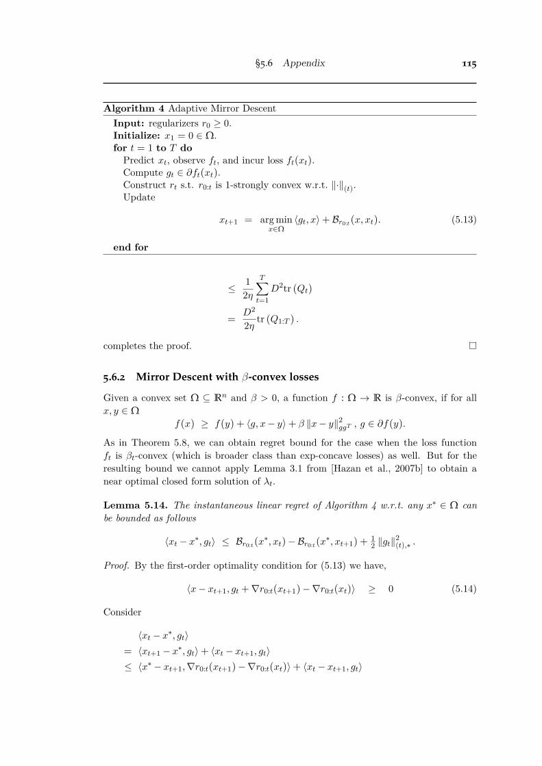
§5.6 Appendix 115
Algorithm 4 Adaptive Mirror DescentInput: regularizers r0 Ø 0.Initialize: x1 = 0 œ W.for t = 1 to T do
Predict xt, observe ft, and incur loss ft(xt).Compute gt œ ˆft(xt).Construct rt s.t. r0:t is 1-strongly convex w.r.t. ηÎ
(t).Update
xt+1 = arg minxœW
Ègt, xÍ + Br0:t(x, xt). (5.13)
end for
Æ 12÷
Tÿ
t=1D2tr
(
Qt)
=
D2
2÷tr(
Q1:T ) .
completes the proof.
5.6.2 Mirror Descent with —-convex losses
Given a convex set W ™ Rn and — > 0, a function f : W æ R is —-convex, if for allx, y œ W
f(x) Ø f(y) + Èg, x ≠ yÍ + — Îx ≠ yÎ2ggT , g œ ˆf(y).
As in Theorem 5.8, we can obtain regret bound for the case when the loss functionft is —t-convex (which is broader class than exp-concave losses) as well. But for theresulting bound we cannot apply Lemma 3.1 from [Hazan et al., 2007b] to obtain anear optimal closed form solution of ⁄t.
Lemma 5.14. The instantaneous linear regret of Algorithm 4 w.r.t. any xú œ W canbe bounded as follows
Èxt ≠ xú, gtÍ Æ Br0:t(xú, xt) ≠ Br0:t(x
ú, xt+1) +12 ÎgtÎ2
(t),ú .
Proof. By the first-order optimality condition for (5.13) we have,
Èx ≠ xt+1, gt + Òr0:t(xt+1) ≠ Òr0:t(xt)Í Ø 0 (5.14)
Consider
Èxt ≠ xú, gtÍ= Èxt+1 ≠ xú, gtÍ + Èxt ≠ xt+1, gtÍÆ Èxú ≠ xt+1, Òr0:t(xt+1) ≠ Òr0:t(xt)Í + Èxt ≠ xt+1, gtÍ

116 Accelerating Optimization for Easy Data
= Br0:t(xú, xt) ≠ Br0:t(x
ú, xt+1) ≠ Br0:t(xt+1, xt) + Èxt ≠ xt+1, gtÍÆ Br0:t(x
ú, xt) ≠ Br0:t(xú, xt+1) ≠ Br0:t(xt+1, xt) +
12 Îxt ≠ xt+1Î2
(t) +12 ÎgtÎ2
(t),úÆ Br0:t(x
ú, xt) ≠ Br0:t(xú, xt+1) +
12 ÎgtÎ2
(t),ú ,
where the first inequality is due to (5.14), the second equality is due to the fact thatÈÒÂ(a) ≠ ÒÂ(b), c ≠ aÍ = BÂ(c, b) ≠ BÂ(c, a) ≠ BÂ(a, b), the second inequality is dueto the fact that Èa, bÍ Æ ÎaÎ ÎbÎú Æ 1
2 ÎaÎ2+
12 ÎbÎ2
ú, and the third inequality is due tothe 1-strong convexity of r0:t w.r.t. ηÎ
(t).
Theorem 5.15. Let ft is —t-convex, ’t œ [T ]. If rt’s are given by
rt(x) = ÎxÎ2ht
, where h0 = In◊n and ht = —tgtgTt for t Ø 1, (5.15)
then the regret of Algorithm 4 w.r.t. any xú œ W is bounded by
Tÿ
t=1ft(xt) ≠ ft(x
ú) Æ 1
4
Tÿ
t=1ÎgtÎ2
h≠10:t
+ Îxú ≠ x1Î22 .
Proof. For the choice of regularizer sequence {rt} given by (5.15), we have r0:t(x) =
ÎxÎ2h0:t
and Br0:t(x, y) =
12
1Ô2 Îx ≠ yÎh0:t
22. Since r0:t is 1-strongly convex w.r.t.Ô
2 ηÎh0:t, we have ηÎ
(t) =Ô
2 ηÎh0:tand ηÎ
(t),ú =
1Ô2 ηÎh≠1
0:t.
For any xú œ W
ft(xt) ≠ ft(xú)
Æ Ègt, xt ≠ xúÍ ≠ —t Îxú ≠ xtÎ2gtgT
t
Æ Br0:t(xú, xt) ≠ Br0:t(x
ú, xt+1) +12 ÎgtÎ2
(t),ú ≠ Îxú ≠ xtÎ2—tgtgT
t
= Îxú ≠ xtÎ2h0:t
≠ Îxú ≠ xt+1Î2h0:t
≠ Îxú ≠ xtÎ2ht+
12 ÎgtÎ2
(t),ú ,
where the first inequality is due to the —t-convexity of ft(·), and the second inequalityis due to Lemma 5.14. By summing all the instantaneous regrets we get
Tÿ
t=1ft(xt) ≠
Tÿ
t=1ft(x
ú)
ÆT
ÿ
t=1
Ó
Îxú ≠ xtÎ2h0:t
≠ Îxú ≠ xtÎ2h0:t≠1
≠ Îxú ≠ xtÎ2ht
Ô
+ Îxú ≠ x1Î2h0
≠ Îxú ≠ xT+1Î2h0:T
+
12
Tÿ
t=1ÎgtÎ2
(t),ú
Æ Îxú ≠ x1Î22 +
14
Tÿ
t=1ÎgtÎ2
h≠10:t
.

§5.6 Appendix 117
Now instead of running Algorithm 4 on the observed sequence of ft’s, we use themodified sequence of loss functions of the form
ft(x) := ft(x) + ⁄tg(x), ⁄t Ø 0, (5.16)
where g(x) is 1-convex. By following the proof of Theorem 5.15 for the modifiedsequence of losses given by (5.16) we obtain the following corollary.Theorem 5.16. Let g(x) be a 1-convex function, A2
= supxœW
g(x) and
B = supxœW
.
.gÕ(x)
.
.
(
gÕ(x)gÕ
(x)T)
≠1 .
Also let ft be —t-convex (—t Ø 0), ’t œ [T ]. If Algorithm 4 is performed on the modifiedfunctions ft’s with the regularizers rt’s given by
rt(x) = ÎxÎ2ht
, where h0 = In◊n, and ht = —tgtgTt + ⁄tg
Õ(xt)g
Õ(xt)
T , for t Ø 1,(5.17)
then for any sequence ⁄1, ..., ⁄T Ø 0, we get
Tÿ
t=1ft(xt) ≠ ft(x
ú) Æ
A
A2+
B2
2
B
⁄1:T +
12
Tÿ
t=1ÎgtÎ2
h≠10:t
+ Îxú ≠ x1Î22 .
Proof. Since ft is —t-convex and g is 1-convex, for any xú œ W we have
{ft(xt) + ⁄tg(xt)} ≠ {ft(xú) + ⁄tg(x
ú)}
= ft(xt) ≠ ft(xú) + ⁄t {g(xt) ≠ g(xú
)}Æ Ègt, xt ≠ xúÍ ≠ —t Îxú ≠ xtÎ2
gtgTt+ ⁄t
Ó
ÈgÕ(xt), xt ≠ xúÍ ≠ Îxú ≠ xtÎ2
gÕ(xt)gÕ
(xt)T
Ô
= Ègt + ⁄tgÕ(xt), xt ≠ xúÍ ≠ Îxú ≠ xtÎ2
—tgtgTt +⁄tgÕ
(xt)gÕ(xt)
T .
By following the similar steps from the proof of Theorem 5.15 we get
Tÿ
t=1ft(xt) + ⁄tg(xt)≠
I
Tÿ
t=1ft(x
ú) + ⁄tg(x
ú)
J
Æ 14
Tÿ
t=1
.
.gt + ⁄tgÕ(xt)
.
.
2h≠1
0:t+ Îxú ≠ x1Î2
2 .
By using the facts that Îx + yÎ2A Æ 2 ÎxÎ2
A + 2 ÎyÎ2A, h0:t < ht < ⁄tgÕ
(xt)gÕ(xt)
T , andÎgÕ
(xt)Î(
gÕ(xt)gÕ
(xt)T)
≠1 Æ B, we have
Tÿ
t=1ft(xt) + ⁄tg(xt) ≠
I
Tÿ
t=1ft(x
ú) + ⁄tg(x
ú)
J
Æ 12
Tÿ
t=1
Ó
ÎgtÎ2h≠1
0:t+ ⁄2
t
.
.gÕ(xt)
.
.
2h≠1
0:t
Ô
+ Îxú ≠ x1Î22
Æ 12
Tÿ
t=1
;
ÎgtÎ2h≠1
0:t+ ⁄2
t
.
.gÕ(xt)
.
.
2(
⁄tgÕ(xt)gÕ
(xt)T)
≠1
<
+ Îxú ≠ x1Î22

118 Accelerating Optimization for Easy Data
Æ 12
Tÿ
t=1ÎgtÎ2
h≠10:t
+
B2
2 ⁄1:T + Îxú ≠ x1Î22 .
By neglecting the g(xt) terms in the L.H.S. and using the fact that g(xú) Æ A2 we get
Tÿ
t=1ft(xt) Æ
Tÿ
t=1ft(x
ú) + A2⁄1:T +
12
Tÿ
t=1ÎgtÎ2
h≠10:t
+ Îxú ≠ x1Î22 +
B2
2 ⁄1:T .
But we cannot apply Lemma 3.1 from [Hazan et al., 2007b] for the above regretbound to obtain a near optimal closed form solution to ⁄t. One could employ anoptimization algorithm to find the optimal ⁄t.

Chapter 6
Conclusion
This thesis studied the problem of bounding the performance of machine learningalgorithms in both statistical and adversarial setting, and designing computationallye�cient algorithms with strong theoretical guarantees.
The major contributions of this thesis are:
• An investigation of the influence of cost terms on the hardness of the cost-sensitiveclassification problem by extending the minimax lower bound analysis for bal-anced binary classification (Theorem 3.6).
• A relationship between the contraction coe�cient of a channel w.r.t. c-primitivef -divergence, and a generalized form of Dobrushin’s coe�cient (Theorem 3.10).
• An increased understanding of contraction coe�cients of binary symmetric chan-nels w.r.t. any symmetric f -divergence (Section 3.3.2).
• A complete characterization of the exp-concavity of any proper composite loss(Proposition 4.4). Using this characterization and the mixability condition ofproper losses (Van Erven et al. [2012]), we showed that it is possible to re-parameterize any —-mixable binary proper loss into a —-exp-concave compositeloss with the same — (Corollary 4.8).
• Analysis of unified update rules of the accelerated online convex optimizationalgorithms (Sections 5.2 and 5.3). Improved regret bounds were achieved byexploiting the easy nature of the sequence of outcomes.
By studying the geometry of prediction problems we have obtained insights intothe factors which conspire to make the problem hard. These insights have enabled usto place bounds on the learning algorithm’s ability to accurately predict the unseendata, and guided us in the design of better solutions.
Throughout the thesis, we have pointed out a number of open questions which wefeel are important. These include the following:
1. Extend the study of the contraction coe�cients of binary symmetric channels(Section 3.3.2) w.r.t. symmetric f -divergences to k-ary symmetric channels (withk > 2) and general f -divergences.
119

120 Conclusion
2. There are some divergences other than f -divergences which satisfy the weak dataprocessing inequality, such as Neyman-Pearson –-divergences ([Polyanskiy andVerdú, 2010; Raginsky, 2011]). Thus it would be interesting to study strong dataprocessing inequalities w.r.t. those divergences as well.
3. Recently people have attempted to relate several types of channel ordering to thestrong data processing inequalities ([Makur and Polyanskiy, 2016; Polyanskiy andWu, 2015]). It is worth to explore the relationship between the statistical defi-ciency based channel ordering (Raginsky [2011]) and the strong data processinginequalities.
4. It would be interesting to study the hardness of the cost-sensitive classifica-tion with example dependent costs ([Zadrozny and Elkan, 2001; Zadrozny et al.,2003]), and the binary classification problem w.r.t. generalized performance mea-sures (Koyejo et al. [2014]) such as arithmetic, geometric and harmonic means ofthe true positive and true negative rates.
5. Further study could be undertaken in applying the cost-sensitive privacy notionto some real-world problems.
6. We illustrated the impact of the choice of substitution function in AggregatingAlgorithm with experiments conducted on a synthetic dataset and a number ofdi�erent real-world data sets (Section 4.4.1). A theoretical understanding of thechoice of substitution functions would be very useful.
7. An e�ciently computable —-exp-concavifying link function for —-mixable multi-class proper losses, is still not known. At least showing a negative result would beworth, for example, showing that it is not possible to exp-concavify a multi-class(with n > 2) square loss with same mixability constant.
8. Develop adaptive and optimistic variants of second order online learning algo-rithms such as online Newton step (Hazan et al. [2007a]), e�ciently using sketch-ing methods (Woodru� [2014]).
Exploring and exploiting the geometric structure of the learning problem will serve asa guiding light in this future work.

Bibliography
Abe, N.; Zadrozny, B.; and Langford, J., 2004. An iterative method for multi-class cost-sensitive learning. In Proceedings of the tenth ACM SIGKDD internationalconference on Knowledge discovery and data mining, 3–11. ACM. (cited on page23)
Abernethy, J.; Bartlett, P. L.; Rakhlin, A.; and Tewari, A., 2008. Optimalstrategies and minimax lower bounds for online convex games. In Proceedings of theAnnual Conference on Learning Theory. (cited on page 97)
Ahlswede, R. and Gács, P., 1976. Spreading of sets in product spaces and hyper-contraction of the Markov operator. The annals of probability, 4 (1976), 925–939.(cited on page 41)
Ali, S. M. and Silvey, S. D., 1966. A general class of coe�cients of divergenceof one distribution from another. Journal of the Royal Statistical Society. Series B(Methodological), (1966), 131–142. (cited on page 15)
Assouad, P., 1983. Deux remarques sur l’estimation. Comptes rendus des séances del’Académie des sciences. Série 1, Mathématique, 296, 23 (1983), 1021–1024. (citedon pages 29, 31, and 33)
Banerjee, A.; Guo, X.; and Wang, H., 2005. On the optimality of conditionalexpectation as a Bregman predictor. IEEE Transactions on Information Theory, 51,7 (2005), 2664–2669. (cited on page 85)
Beck, A. and Teboulle, M., 2003. Mirror descent and nonlinear projected subgra-dient methods for convex optimization. Operations Research Letters, 31, 3 (2003),167–175. (cited on page 100)
Bhatia, K.; Jain, P.; Kamalaruban, P.; and Kar, P., 2016. E�cient and con-sistent robust time series analysis. arXiv preprint arXiv:1607.00146, (2016). (citedon page 3)
Blackwell, D., 1951. Comparison of experiments. In Proceedings of the secondBerkeley symposium on mathematical statistics and probability, vol. 1, 93–102. (citedon page 5)
Boyd, S. and Vandenberghe, L., 2004. Convex optimization. Cambridge universitypress. (cited on page 102)
121

122 BIBLIOGRAPHY
Buja, A.; Stuetzle, W.; and Shen, Y., 2005. Loss functions for binary classprobability estimation and classification: Structure and applications. (2005). (citedon pages 65, 69, and 95)
Cardie, C. and Nowe, N., 1997. Improving minority class prediction using case-specific feature weights. In Proceedings of the Fourteenth International Conferenceon Machine Learning, 57–65. (cited on page 40)
Cesa-Bianchi, N.; Conconi, A.; and Gentile, C., 2004. On the generalizationability of on-line learning algorithms. IEEE Transactions on Information Theory,50, 9 (2004), 2050–2057. (cited on page 112)
Cesa-Bianchi, N. and Lugosi, G., 2006. Prediction, learning, and games. Cam-bridge university press. (cited on pages 2 and 68)
Chatzikokolakis, K.; Andrés, M. E.; Bordenabe, N. E.; and Palamidessi,C., 2013. Broadening the scope of di�erential privacy using metrics. In InternationalSymposium on Privacy Enhancing Technologies Symposium, 82–102. Springer. (citedon page 60)
Chiang, C.-K.; Yang, T.; Lee, C.-J.; Mahdavi, M.; Lu, C.-J.; Jin, R.; andZhu, S., 2012. Online optimization with gradual variations. In Proceedings of theAnnual Conference on Learning Theory, 6.1–6.20. (cited on pages 3, 98, 100, 101,102, 103, and 105)
Cohen, J. E.; Iwasa, Y.; Rautu, G.; Ruskai, M. B.; Seneta, E.; and Zbaganu,G., 1993. Relative entropy under mappings by stochastic matrices. Linear algebraand its applications, 179 (1993), 211–235. (cited on pages 23, 41, and 43)
Csiszár, I., 1972. A class of measures of informativity of observation channels. Peri-odica Mathematica Hungarica, 2, 1-4 (1972), 191–213. (cited on page 15)
Dawid, A. P., 2007. The geometry of proper scoring rules. Annals of the Institute ofStatistical Mathematics, 59, 1 (2007), 77–93. (cited on page 5)
DeGroot, M. H., 1962. Uncertainty, information, and sequential experiments. TheAnnals of Mathematical Statistics, 33 (1962), 404–419. (cited on page 5)
Devroye, L.; Györfi, L.; and Lugosi, G., 2013. A probabilistic theory of patternrecognition, vol. 31. Springer Science & Business Media. (cited on page 25)
Do, C. B.; Le, Q. V.; and Foo, C.-S., 2009. Proximal regularization for onlineand batch learning. In Proceedings of the 26th Annual International Conference onMachine Learning, 257–264. ACM. (cited on pages 108 and 110)
Dobrushin, R. L., 1956a. Central limit theorem for nonstationary Markov chains. I.Theory of Probability & Its Applications, 1, 1 (1956), 65–80. (cited on page 41)

BIBLIOGRAPHY 123
Dobrushin, R. L., 1956b. Central limit theorem for nonstationary Markov chains. II.Theory of Probability & Its Applications, 1, 4 (1956), 329–383. (cited on page 41)
Dragomir, S. S., 2000. Some Gronwall type inequalities and applications. RGMIAMonographs, Victoria University, Australia, 19 (2000). (cited on page 89)
Duchi, J., 2016; accessed March 30, 2017. Statistics and information theory. https://stanford.edu/class/stats311/. (cited on page 29)
Duchi, J.; Hazan, E.; and Singer, Y., 2011. Adaptive subgradient methods foronline learning and stochastic optimization. The Journal of Machine Learning Re-search, 12 (2011), 2121–2159. (cited on pages 3, 98, 103, 105, 106, and 114)
Duchi, J.; Jordan, M.; and Wainwright, M., 2013. Local privacy and statisticalminimax rates. In 54th Annual Symposium on Foundations of Computer Science(FOCS), 429–438. IEEE. (cited on pages 57 and 58)
Dwork, C., 2008. Di�erential privacy: A survey of results. In International Conferenceon Theory and Applications of Models of Computation, 1–19. Springer. (cited onpage 58)
Dwork, C.; McSherry, F.; Nissim, K.; and Smith, A., 2006. Calibrating noise tosensitivity in private data analysis. In Theory of Cryptography Conference, 265–284.Springer. (cited on page 57)
Eguchi, S. and Copas, J., 2001. Recent developments in discriminant analysis froman information geometric point of view. Journal of the Korean Statistical Society, 30(2001), 247–264. (cited on page 15)
Elkan, C., 2001. The foundations of cost-sensitive learning. In International jointconference on artificial intelligence, vol. 17, 973–978. Lawrence Erlbaum AssociatesLtd. (cited on page 40)
Gneiting, T. and Raftery, A. E., 2007. Strictly proper scoring rules, prediction,and estimation. Journal of the American Statistical Association, 102, 477 (2007),359–378. (cited on page 69)
Grünwald, P. D. and Dawid, A. P., 2004. Game theory, maximum entropy, min-imum discrepancy and robust Bayesian decision theory. Annals of Statistics, 32(2004), 1367–1433. (cited on page 5)
Guntuboyina, A.; Saha, S.; and Schiebinger, G., 2014. Sharp inequalities forf -divergences. IEEE Transactions on Information Theory, 60, 1 (2014), 104–121.(cited on page 19)
Hand, D. J., 1994. Deconstructing statistical questions. Journal of the Royal Statis-tical Society, Series A (Statistics in Society), 157, 3 (1994), 317–356. (cited on page65)

124 BIBLIOGRAPHY
Hand, D. J. and Vinciotti, V., 2003. Local versus global models for classificationproblems: Fitting models where it matters. The American Statistician, 57, 2 (2003),124–131. (cited on page 65)
Harremoes, P. and Vajda, I., 2011. On pairs of f -divergences and their joint range.IEEE Transactions on Information Theory, 57, 6 (2011), 3230–3235. (cited on page19)
Haussler, D.; Kivinen, J.; and Warmuth, M. K., 1998. Sequential prediction ofindividual sequences under general loss functions. IEEE Transactions on InformationTheory, 44, 5 (1998), 1906–1925. (cited on page 85)
Hazan, E.; Agarwal, A.; and Kale, S., 2007a. Logarithmic regret algorithms foronline convex optimization. Machine Learning, 69, 2-3 (2007), 169–192. (cited onpages 2, 98, and 120)
Hazan, E. and Kale, S., 2010. Extracting certainty from uncertainty: Regretbounded by variation in costs. Machine Learning, 80, 2-3 (2010), 165–188. (citedon page 100)
Hazan, E.; Rakhlin, A.; and Bartlett, P. L., 2007b. Adaptive online gradientdescent. In Advances in Neural Information Processing Systems, vol. 20, 65–72.(cited on pages 3, 98, 99, 106, 108, 115, and 118)
Hiriart-Urruty, J.-B. and Lemaréchal, C., 1993. Convex analysis and mini-mization algorithms I: Fundamentals, vol. 305. Springer. (cited on pages 6 and 67)
Isaacson, D. L. and Madsen, R. W., 1976. Markov chains, theory and applications,vol. 4. Wiley New York. (cited on page 41)
Kairouz, P.; Oh, S.; and Viswanath, P., 2014. Extremal mechanisms for localdi�erential privacy. In Advances in neural information processing systems, vol. 27,2879–2887. (cited on page 59)
Kakade, S. M. and Tewari, A., 2009. On the generalization ability of onlinestrongly convex programming algorithms. In Advances in Neural Information Pro-cessing Systems, vol. 22, 801–808. (cited on page 112)
Kalnishkan, Y. and Vyugin, M. V., 2005. The weak aggregating algorithm andweak mixability. In Proceedings of the Annual Conference on Learning Theory, 188–203. Springer. (cited on page 68)
Kivinen, J. and Warmuth, M. K., 1999. Averaging expert predictions. In Proceed-ings of the Annual Conference on Learning Theory, 153–167. Springer. (cited onpages 3, 65, 70, 78, and 79)
Komiya, H., 1988. Elementary proof for Sion’s minimax theorem. Kodai MathematicalJournal, 11, 1 (1988), 5–7. (cited on page 12)

BIBLIOGRAPHY 125
Koyejo, O. O.; Natarajan, N.; Ravikumar, P. K.; and Dhillon, I. S., 2014.Consistent binary classification with generalized performance metrics. In Advancesin Neural Information Processing Systems, vol. 27, 2744–2752. (cited on pages 39and 120)
Le Cam, L., 1964. Su�ciency and approximate su�ciency. The Annals of Mathemat-ical Statistics, (1964), 1419–1455. (cited on page 5)
Le Cam, L., 2012. Asymptotic methods in statistical decision theory. Springer Science& Business Media. (cited on pages 5, 8, 29, and 31)
Liese, F. and Vajda, I., 2006. On divergences and informations in statistics andinformation theory. IEEE Transactions on Information Theory, 52, 10 (2006), 4394–4412. (cited on page 17)
Makur, A. and Polyanskiy, Y., 2016. Comparison of channels: criteria for domi-nation by a symmetric channel. ArXiv:1609.06877 (cs.IT). (cited on pages 45, 62,and 120)
Massart, P. and Nédélec, É., 2006. Risk bounds for statistical learning. TheAnnals of Statistics, (2006), 2326–2366. (cited on pages 23, 34, and 39)
McMahan, H. B., 2014. A survey of algorithms and analysis for adaptive onlinelearning. ArXiv:1403.3465 (cs.LG). (cited on pages 98 and 99)
Mitchell, T., 1997. Machine Learning. McGraw-Hill, Inc. (cited on page 1)
Mohri, M. and Yang, S., 2015. Accelerating optimization via adaptive prediction.arXiv preprint, (2015). ArXiv:1509.05760 (stat.ML). (cited on page 99)
Mohri, M. and Yang, S., 2016. Accelerating online convex optimization via adaptiveprediction. In Artificial Intelligence and Statistics, 848–856. (cited on page 106)
Neyman, J. and Pearson, E., 1933. On the problem of the most e�cient tests ofstatistical hypotheses. Philosophical Transactions of the Royal Society of LondonSeries A, 231 (1933), 289–337. (cited on page 15)
Orabona, F.; Jie, L.; and Caputo, B., 2010. Online-batch strongly convex multikernel learning. In Proceedings of IEEE Conference on Computer Vision and PatternRecognition (CVPR), 787–794. IEEE. (cited on page 110)
Paz, A., 1971. Introduction to probabilistic automata (Computer science and appliedmathematics). Academic Press, Inc. (cited on page 41)
Polyanskiy, Y. and Verdú, S., 2010. Arimoto channel coding converse and Rényidivergence. In 48th Annual Conference on Communication, Control, and Computing(Allerton), 1327–1333. IEEE. (cited on pages 62 and 120)
Polyanskiy, Y. and Wu, Y., 2015. Strong data-processing inequalities for channelsand Bayesian networks. ArXiv:1508.06025 (cs.IT). (cited on pages 62 and 120)

126 BIBLIOGRAPHY
Polyanskiy, Y. and Wu, Y., 2016; accessed March 30, 2017. Lecture notes oninformation theory. http://people.lids.mit.edu/yp/homepage/data/itlectures_v4.pdf.(cited on page 19)
Raginsky, M., 2011. Shannon meets Nlackwell and Le Cam: Channels, codes, andstatistical experiments. In International Symposium on Information Theory (ISIT),1220–1224. IEEE. (cited on pages 62, 63, and 120)
Raginsky, M., 2014. Strong data processing inequalities and „-Sobolev inequalitiesfor discrete channels. ArXiv:1411.3575 (cs.IT). (cited on pages 2, 41, 43, and 44)
Raginsky, M., 2015; accessed March 30, 2017. Minimax lower bounds (statisticallearning theory). http://maxim.ece.illinois.edu/teaching/fall15b/notes/minimax.pdf.(cited on page 30)
Rakhlin, A. and Sridharan, K., 2012. Online learning with predictable sequences.arXiv preprint, (2012). ArXiv:1208.3728 (stat.ML). (cited on pages 98 and 100)
Reid, M. D. and Williamson, R. C., 2010. Composite binary losses. Journal ofMachine Learning Research, 11 (2010), 2387–2422. (cited on page 75)
Reid, M. D. and Williamson, R. C., 2011. Information, divergence and risk forbinary experiments. Journal of Machine Learning Research, 12 (2011), 731–817.(cited on pages 1, 5, 17, 46, and 69)
Rockafellar, R. T., 1970. Convex analysis. Princeton University Press. (cited onpages 5, 6, and 66)
Scott, C. et al., 2012. Calibrated asymmetric surrogate losses. Electronic Journalof Statistics, 6 (2012), 958–992. (cited on page 28)
Shalev-Shwartz, S., 2011. Online learning and online convex optimization. Foun-dations and Trends in Machine Learning, 4, 2 (2011), 107–194. (cited on pages 3,97, and 98)
Srebro, N.; Sridharan, K.; and Tewari, A., 2011. On the universality of onlinemirror descent. In Advances in neural information processing systems, vol. 24, 2645–2653. (cited on page 100)
Torgersen, E., 1991. Comparison of statistical experiments. Cambridge UniversityPress. (cited on pages 5, 8, and 15)
Tsybakov, A. B., 2004. Optimal aggregation of classifiers in statistical learning.Annals of Statistics, 32 (2004), 135–166. (cited on page 34)
Tsybakov, A. B., 2009. Introduction to Nonparametric Estimation. Springer. (citedon pages 19 and 29)
van Erven, T., 2012. From exp-concavity to mixability. http://www.timvanerven.nl/blog/2012/12/from-exp-concavity-to-mixability/. (cited on pages 65 and 71)

BIBLIOGRAPHY 127
Van Erven, T.; Reid, M. D.; and Williamson, R. C., 2012. Mixability is Bayesrisk curvature relative to log loss. Journal of Machine Learning Research, 13, 1(2012), 1639–1663. (cited on pages 66, 67, 69, 77, 96, and 119)
Vapnik, V., 1998. Statistical learning theory. Wiley New York. (cited on page 1)
Vapnik, V. and Chervonenkis, A. Y., 1971. On the uniform convergence of relativefrequencies of events to their probabilities. Theory of Probability and its Applications,16, 2 (1971), 264. (cited on page 63)
Vapnik, V. N. and Chervonenkis, A. Y., 1974. Theory of Pattern Recognition [inRussian]. Nauka. (cited on page 34)
Von Neumann, J. and Morgenstern, O., 1944. Theory of games and economicbehavior. Princeton University Press. (cited on page 5)
Vovk, V., 1995. A game of prediction with expert advice. In Proceedings of theAnnual Conference on Learning Theory, 51–60. ACM. (cited on pages 2, 3, 65, 68,70, and 78)
Vovk, V., 2001. Competitive on-line statistics. International Statistical Review, 69, 2(2001), 213–248. (cited on pages 71, 78, and 80)
Vovk, V. and Zhdanov, F., 2009. Prediction with expert advice for the Brier game.Journal of Machine Learning Research, 10 (2009), 2445–2471. (cited on pages 68and 84)
Wald, A., 1949. Statistical decision functions. The Annals of Mathematical Statistics,11 (1949), 165–205. (cited on page 5)
Warner, S. L., 1965. Randomized response: A survey technique for eliminatingevasive answer bias. Journal of the American Statistical Association, 60, 309 (1965),63–69. (cited on page 57)
Wasserman, L. and Zhou, S., 2010. A statistical framework for di�erential privacy.Journal of the American Statistical Association, 105, 489 (2010), 375–389. (cited onpages 57 and 58)
Williamson, R. C., 2014. The geometry of losses. In Proceedings of the AnnualConference on Learning Theory, 1078–1108. (cited on pages 73, 78, and 79)
Williamson, R. C.; Vernet, E.; and Reid, M. D., 2016. Composite multiclasslosses. Journal of Machine Learning Research, 17, 223 (2016), 1–52. (cited on pages65, 69, 73, 75, and 87)
Woodruff, D. P., 2014. Sketching as a tool for numerical linear algebra. Foundationsand Trends in Theoretical Computer Science, 10, 1–2 (2014), 1–157. (cited on page120)

128 BIBLIOGRAPHY
Yang, Y. and Barron, A., 1999. Information-theoretic determination of minimaxrates of convergence. Annals of Statistics, 27 (1999), 1564–1599. (cited on page 29)
Yu, B., 1997. Assouad, Fano, and Le Cam. In Festschrift for Lucien Le Cam, 423–435.Springer. (cited on page 29)
Zadrozny, B. and Elkan, C., 2001. Learning and making decisions when costsand probabilities are both unknown. In Proceedings of the 7th International Confer-ence on Knowledge discovery and data mining, 204–213. ACM. (cited on pages 39and 120)
Zadrozny, B.; Langford, J.; and Abe, N., 2003. Cost-sensitive learning by cost-proportionate example weighting. In Proceedings of the Third IEEE InternationalConference on Data Mining, 435–442. IEEE. (cited on pages 39 and 120)
Zinkevich, M., 2003. Online convex programming and generalized infinitesimal gra-dient ascent. In Proceedings of the International Conference on Machine Learning,928–936. (cited on pages 2 and 98)