HAL Id: hal-03260357https://hal.inria.fr/hal-03260357

Preprint submitted on 14 Jun 2021

HAL is a multi-disciplinary open accessarchive for the deposit and dissemination of sci-entific research documents, whether they are pub-lished or not. The documents may come fromteaching and research institutions in France orabroad, or from public or private research centers.

L’archive ouverte pluridisciplinaire HAL, estdestinée au dépôt et à la diffusion de documentsscientifiques de niveau recherche, publiés ou non,émanant des établissements d’enseignement et derecherche français ou étrangers, des laboratoirespublics ou privés.

Towards Optimally Weighted Physics-Informed NeuralNetworks in Ocean Modelling

Taco de Wolff, Hugo Carrillo, Luis Martí, Nayat Sanchez-Pi

To cite this version:Taco de Wolff, Hugo Carrillo, Luis Martí, Nayat Sanchez-Pi. Towards Optimally Weighted Physics-Informed Neural Networks in Ocean Modelling. 2021. hal-03260357

Towards Optimally Weighted Physics-Informed NeuralNetworks in Ocean Modelling

Taco de Wolff, Hugo Carrillo, Luis Martí & Nayat Sánchez-PiInria Chile Research Center

Av. Apoquindo 2827, piso 12, Las Condes, Santiago, Chiletaco.dewolff,hugo.carrillo,luis.marti,nayat.sanchez-pi@inria.cl

Abstract

The carbon pump of the world’s ocean plays a vital role in the biosphere andclimate of the earth, urging improved understanding of the functions and influencesof the ocean for climate change analyses. State-of-the-art techniques are required todevelop models that can capture the complexity of ocean currents and temperatureflows. This work explores the benefits of using physics-informed neural networks(PINNs) for solving partial differential equations related to ocean modeling; suchas the Burgers, wave, and advection-diffusion equations. We explore the trade-offsof using data vs. physical models in PINNs for solving partial differential equations.PINNs account for the deviation from physical laws in order to improve learningand generalization. We observed how the relative weight between the data andphysical model in the loss function influence training results, where small data setsbenefit more from the added physics information.

1 Introduction

The ocean plays a key role in the biosphere [18]. It regulates the carbon cycle by absorbing emittedCO2 through the biological pump and dissipates a large part of the heat that is retained in theatmosphere by the remaining CO2 and other greenhouse gases. The biological pump is driven byphotosynthetic microalgae, herbivores, and decomposing bacteria. Understanding the drivers ofmicro- and macroorganisms in the ocean is of paramount importance to understand the functioning ofecosystems and the efficiency of the biological pump in sequestering carbon and thus abating climatechange.

Similarly, there is also a clear scientific consensus about the effects of climate change on the ocean.Changes like the shift in temperature, an increase of acidification, deoxygenation of water masses,perturbations in nutrient availability, and biomass productivity to mention a few, have a dramaticimpact on almost all forms of life in the ocean with further consequences on food security, ecosystemservices, and the well-being of coastal communities and humankind in general.

Consequently, we end up with a cyclic dependency: to understand and create strategies to mitigateclimate change it is of primordial importance to understand the ocean and to understand the ocean it isnecessary to understand how climate change is impacting it. Therefore, this is not only an urgent butalso a scientifically demanding task that must be addressed with a cohort approach involving differentscientific areas: state-of-the-art artificial intelligence, machine learning, applied math, modelling, andsimulation, and of course marine biology and oceanography.

That is why it can be hypothesized that it is necessary to develop new state-of-the-art artificialintelligence, machine learning, and mathematical modelling tools that will enable us to moveforward with the understanding of our ocean and to understand, predict, and hopefully mitigatethe consequences of climate change.

Preprint. Under review.

The ocean is mostly a fluid in almost permanent movement – subjected to currents, tides, waves andother interactions – where different where organisms, atmosphere, and continents interact. Modellingoceanic fluid dynamics is essential but also very expensive in the computational sense. Mathematicalmodels like the Navier-Stokes equations [21] can express most of the processes of interest [14].However, the high computational cost involved in applying them with the correct precision levelmakes their application intractable. Machine learning (ML) and, in particular, neural networks are acompetitive alternative. However, these approaches in general require a large amount of data to serveas examples for the learning process. In oceanographic research, obtaining data is challenging andexpensive. The approach of hybrid models seems to be a good alternative to tackle this problem.

Physics-informed neural networks (PINNs) [16] are a hybrid approach that take into account adata-based neural network model and a physics-informed mechanistic model, which are two differentparadigms. They offer a framework where existing knowledge about a physical phenomenon andempirical data gathered about it. This general concept has been previously explored and is knownas data assimilation [25], but PINNs bring a novel and sound approach to consolidate the existingmodels and sampled data. This feature makes PINNs particularly appealing for the above-describedproblems and has lead to some preliminary studies [5, 13].

Furthermore, it could be argued that by incorporating a rule that promotes the consistency of theneural with a priori existing knowledge, the internal representations created during the training phasecould be easier to understand and interpret by domain experts and, therefore, become not only amodelling but a research tool with a more broad impact.

This paper deals with the problem of predicting values of physical laws at given points in space andtime relying on PINNs with a focus on ocean modelling. Our main goal is provide a first attempt-to the best of our knowledge- at determining what is the importance and relevance of the physicalcomponent in PINNs in improving the predictive power of a neural network concerning the amountof data available. By answering this question we aim to find a procedure for efficient configuration ofparameters with numerical experiments inferred from the characteristics of the problem and the dataavailable.

The contributions of this papers are:

1. to study the influence of the physics information and the scenarios where using it is moreeffective,

2. a first step towards the automatic parameterization of PINNs using oceanographic modellingas test case, and

3. we study the effects of other hyperparameters as the length and width of the neural networkand activation functions on the optimal weight.

The rest of this paper is organized as follows. In Section 2 we present a brief rationale regardingthe context of the paper, PINNs, modelling ocean fluids and the particular equations that we want toaddress (see 2.1). After that, in Section 3, we deal with the theoretical aspects of our work. Then, inSection 4, we describe and analyze the experimental studies involving PINNs for the estimation ofthe solution and parameters of the PDEs. Finally, in Section 6 we put forward our conclusions ofoutline out future work.

2 Foundations

High-dimensional partial differential equations (PDEs) [17] are a common fixture in areas as diverseas physics, chemistry, engineering, finance, etc. Their enormous success has been hampered by itslimited computational viability. Numerical methods for solving PDEs such as finite difference orfinite element methods become infeasible in higher dimensions due to the explosion in the number ofgrid points and the demand for reduced time step sizes.

Addressing PDE scalability by approximating them by neural networks has been considered invarious forms either by creating a training data set by directly sampling from an a priori fixed meshor by directly sampling the solution in a random manner (see [19] for an overview). Consequently, adatabase of synthetic data coming from the numerical resolution of PDE-based models is generatedon a broad range of scenarios. These data sets are then used to train and validate deep neural networksas in [4, 6].

2

These approaches have the limitation of high computational costs for creating such data sets. Tosubvert the high computational costs, PINNs were recently proposed by [16] as a hybrid approachthat considers a process where a source of physical knowledge in the form of PDEs is available. Theyspecify the problem of training the neural networks as a multi-objective learning task, where wewant to minimize the error with the data as well as the error with a physical law. Now we have threeproblems instead of one: minimizing the error with the data, minimizing the error with the physicallaw, and the combination of training for both objectives. [16] solves this by incorporating a physicsloss term to the loss function, including a relative weight between both loss terms.

As it is a recent topic, there is not much literature about weighted PINNs. Having optimal weights forthe loss functions in PINNs could help us to improve the performance of deep learning solvers forPDEs and so make the computations cheaper than regular PINNs. In [23], the authors propose optimalweights for linear PDEs under the knowledge of boundary values and the differential equation. Theyuse the structure and properties of the PDEs studied.

In [26], the authors propose a self-adaptive loss balanced PINNs (lbPINNs) to solve the incompressibleNavier-Stokes equation by an empirical search of the weights. In [24], the authors also choseempirically the weights to the loss functions in PINNs for study myocardial perfusion in MRI. On theother hand, in [8] the authors evaluate the different results given by a few amount of weights in theloss functions for the advection-diffusion equation.

In this work, we study the influence of the weight on a validation quality metric, in particular therelative error of the neural network solution. In addition, we study the effects of other hyperparametersas the length and width of the neural network and activation functions on the optimal weight.

2.1 Model equations related to the Ocean

The ocean is characterized by its fluid nature. It is constituted mainly by water in different formsthat is subjected to the effects of waves created by wind, currents, tides, among others. Therefore, inorder to understand the ocean it is necessary to take into account this fundamental characteristic andto model it and the intervening phenomena. This gains particular relevance with the emergence of theclimate change phenomenon and, therefore, we need trying to model, forecast and device policies toattempt to mitigate its effects.

Modelling oceanic fluid dynamics is essential but also very expensive in the computational sense.Mathematical models like the Navier-Stokes equations [21] can express most of the processes ofinterest. However, the high computational cost involved in applying them with the correct precisionlevel makes their application intractable.

There are a number of equations that are of particular interest when modelling the ocean that are thefocus of this work. In particular,

• Burgers equation [3]: appears often as a simplification to understand the main properties ofthe Navier-Stokes equations. It is a one-dimensional equation where the pressure is neglectedbut the effects of the nonlinear and viscous terms remain, hence as in the Navier-Stokesequations a Reynolds number can be defined [15]. Hence, it is frequently used as a tool thatis used to understand some of the inside behavior of the general problem.

• Wave equation [20]: in this work we include the wave equation since, under certain suitableconditions, it can be seen as a reduced model of the shallow-water equation which modelsthe water height behavior in coasts and channels.

• Advection-diffusion equations [22]: models the behavior of temperature in a fluid, consider-ing its velocity in the advective term and a diffusion phenomenon of the temperature.

For the sake of briefness, a full description of these equations along with the details about how theyare used in our experiments is given on Section 4.

In this work we study the behavior of the relative error (validation loss) with respect to the weightin the physical part, for Burgers, wave, and advection-diffusion equations. In [8] the authors studyPINNs for advection-difussion equations, also considering different weights. On the other hand, itis very usual in the literature to find only the use of boundary and initial conditions as data, while alarge amount of interior data is considered for data driven discovery of PDEs.

3

Neural network Physics information

x

y

t...

...

u

v

I

∂/∂x

∂/∂y

∂2/∂x2

etc.

f

`data(u, u, v, v)

`physics(f)

` = (1− λ)`data + λ`physics

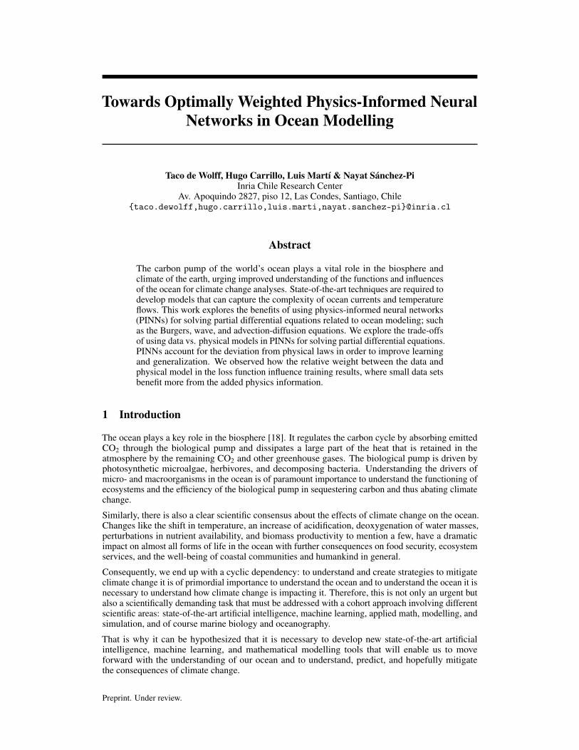
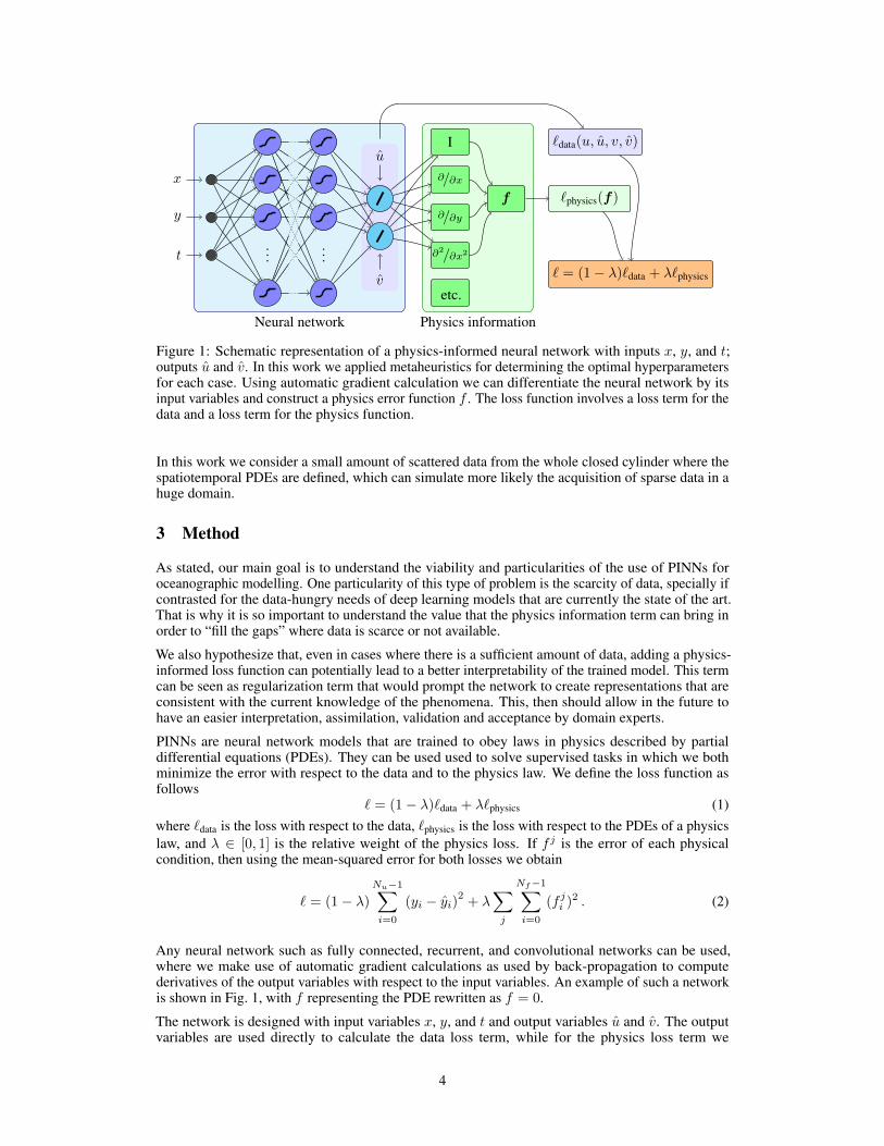
Figure 1: Schematic representation of a physics-informed neural network with inputs x, y, and t;outputs u and v. In this work we applied metaheuristics for determining the optimal hyperparametersfor each case. Using automatic gradient calculation we can differentiate the neural network by itsinput variables and construct a physics error function f . The loss function involves a loss term for thedata and a loss term for the physics function.

In this work we consider a small amount of scattered data from the whole closed cylinder where thespatiotemporal PDEs are defined, which can simulate more likely the acquisition of sparse data in ahuge domain.

3 Method

As stated, our main goal is to understand the viability and particularities of the use of PINNs foroceanographic modelling. One particularity of this type of problem is the scarcity of data, specially ifcontrasted for the data-hungry needs of deep learning models that are currently the state of the art.That is why it is so important to understand the value that the physics information term can bring inorder to “fill the gaps” where data is scarce or not available.

We also hypothesize that, even in cases where there is a sufficient amount of data, adding a physics-informed loss function can potentially lead to a better interpretability of the trained model. This termcan be seen as regularization term that would prompt the network to create representations that areconsistent with the current knowledge of the phenomena. This, then should allow in the future tohave an easier interpretation, assimilation, validation and acceptance by domain experts.

PINNs are neural network models that are trained to obey laws in physics described by partialdifferential equations (PDEs). They can be used used to solve supervised tasks in which we bothminimize the error with respect to the data and to the physics law. We define the loss function asfollows

` = (1− λ)`data + λ`physics (1)where `data is the loss with respect to the data, `physics is the loss with respect to the PDEs of a physicslaw, and λ ∈ [0, 1] is the relative weight of the physics loss. If f j is the error of each physicalcondition, then using the mean-squared error for both losses we obtain

` = (1− λ)

Nu−1∑i=0

(yi − yi)2 + λ∑j

Nf−1∑i=0

(f ji )2 . (2)

Any neural network such as fully connected, recurrent, and convolutional networks can be used,where we make use of automatic gradient calculations as used by back-propagation to computederivatives of the output variables with respect to the input variables. An example of such a networkis shown in Fig. 1, with f representing the PDE rewritten as f = 0.

The network is designed with input variables x, y, and t and output variables u and v. The outputvariables are used directly to calculate the data loss term, while for the physics loss term we

4

differentiate the variables with respect to the input variables as needed for the physics loss function.Observe that the neural network must have input variables that correspond to the physics law’sderivative terms. That is, if ∂u/∂x is part of our physics loss function, then x must be an input variableand u an output variable of our neural network.

The objective is to train both in a supervisory manner with measured or simulated data (i. e. `data),as well as training to minimize the departure from the physics law. The `physics term ensures thatthe neural network generalizes better for unseen data by preventing overfitting. The physics lossencourages that the output variables are not just trained to a local region around the input values ofthe given data, but that also their first and/or second-degree derivations (depending on the PDEs)match with our physical understanding of the model thus spurring better predictive power outside theregion of the training data.

We denote Nl ×Ml as a multi-layer perceptron (MLP) of Nl hidden layers and Ml neurons per layer.As part of the experimentation we assess different activation functions. As our optimization problemis non-convex, the stochastic gradient-descent Adam optimizer was used [10] with different learningrates depending on the problem. The weights of the neural network are initialized randomly usingXavier’s initialization method [7]. As we intend to analyze how activation functions play a role inlearning the derivations of PDEs the tanh, GELU, Softplus, LogSigmoid, Sigmoid, TanhShrink,CELU, Softsign, and ReLU activation functions.

We select a sample subset (Xi, Yi)∀i ∈ [0, Nu − 1] at random from the entire solution space fortraining the data loss, with Xi ∈ RD the D features and Yi ∈ RP the labels of dimension P . For thephysics loss we select a subset Xi∀i ∈ [0, Nf − 1] at random for which we evaluate the PDE error.Note that for the physics loss the solution is not needed, allowing applications to be able to train evenwhen few data are available of the solution. In general we pick Nu Nf .

4 Experiments

As stated in Section 2, we consider three models: the first ones, the Burgers equation, is a nonlinearone-dimensional and the other two, wave, and advection-diffusion equations, are linear and twodimensional PDEs.

4.1 Datasets preparation

In order to generate data for training, validation, and testing, we simulate the PDEs using a Fourierspectral method for the one dimensional model, finite element methods (FEM) for the wave equationand the explicit analytical solution for the advection-diffusion equation. Simulations for the two-dimensional problems were performed using FEniCS [1].

Burgers equation We consider the following Burgers equation

∂u

∂t+ u

∂u

∂x= ν

∂2u

∂x2, (3)

where ν is a diffusion coefficient. This equation usually appears in the context of fluid mechanics, andmore specifically models one-dimensional internal waves in deep ocean. It represents a hyperbolicconservation law as ν → 0 and it is the simplest model for analyzing the effect of nonlinear advectionand diffusion in a combined way. Notice that the Burgers equation can be written as a physics lossterm of (2) as fBurgers[u] = 0.

We simulated the Burgers equation in the spatiotemporal domain [0, L] × [0, T ], using a Fourierspectral method as described in [2].

The diffusion coefficient is taken as ν =

(0.01

π

).

We consider the initial condition

u(x, 0) = − sin(πx), with x ∈ (−1, 1) , (4)

and boundary conditions

u(1, t) = u(−1, t) = 0, with t ∈ (0, 1) , (5)

5

with N = 512 spatial points in a uniform grid in [−1, 1] and 100 points in time defined in a uniformgrid in [0, 1].

Wave equation In this case, we consider the wave equation

∂2η

∂t2−∇ · (H∇η) = 0 , (6)

where η : Ω× R+0 → R represents the superficial fluctuations of a water container or channel and

H : Ω → R+0 is the depth of the water from a reference level. This equation can be written as

fwaves[η,H] = 0. This is where the physics loss is taken from for this PDE.

We simulate the wave equation in a rectangular domain in the time interval ]0, Tf [, with Dirichletboundary conditions for η as

η = 0, on ∂Ω× ]0, Tf [ , (7)

and initial conditions on Ω

η(x, y, 0) = exp(−10 ·

((x− 0.5)2 + (y − 0.75)2

)),

∂η∂t (x, y, 0) = 0 .

(8)

On the other hand, the depth H is given by

H(x, y) = (1− x)(2− sin(3πy)) in Ω . (9)

We implement FEM in this equation considering Lagrange finite elements of degree 1. The timescheme is explicit and Tf = 1.0, n = 100.

Advection-diffusion equation We consider the advection-diffusion equation for heat transfer,assuming that the diffusion coefficient is constant, there are no sources nor sinks of heat, and thetemperature depends only on x, y, and t, that is,

∂T

∂t= D∇2T − u · ∇T , (10)

where T : Ω× R+0 → R is the temperature in K, D = 0.1 m2

s is the thermal diffusivity considered inthis work, and u : Ω× R+

0 → R2 the velocity field in ms . The equation can be written as a physics

loss term asfAD[u, v, T ] = 0 . (11)

We simulate the advection-diffusion equation in Ω× (0, Tf ) where Ω = (0, Lx)× (0, Ly), whereLx = Ly = 1.0 and Tf = 1.0. In addition, D = 0.02, u = (cos(φ) and v = sin(φ)), whereφ = 22.5. We consider the following initial conditions

T (x, y, 0) = exp

(−x

2 + y2

D

), inΩ , (12)

and boundary condition

T (x, y, t) =1

4t+ 1exp

[−x

2 + y2 + t2(u2 + v2)− 2t(xu+ yv)

D(4t+ 1)

]on ∂Ω . (13)

As the coefficients are constant and the domain is a square, we are able to solve this linear equationby known analytic methods. The explicit solution of this equation is

T (x, y, t) =1

4t+ 1exp

[−x

2 + y2 + t2(u2 + v2)− 2t(xu+ yv)

D(4t+ 1)

], (14)

so we generate this solution in a uniform unit square mesh with 40 points in each spatial dimension.

6

10 3

10 2

10 1

100

Valid

atio

n lo

ss

Burgers Nu = 500 AdvDif Nu = 2500

10 3

10 2

10 1

100Waves Nu = 500

10 3

10 2

10 1

100

Valid

atio

n lo

ss

Burgers Nu = 200 AdvDif Nu = 500

10 3

10 2

10 1

100Waves Nu = 200

0.0 0.2 0.4 0.6 0.8 1.0Lambda

10 3

10 2

10 1

100

Valid

atio

n lo

ss

Burgers Nu = 100

0.0 0.2 0.4 0.6 0.8 1.0Lambda

AdvDif Nu = 100

0.0 0.2 0.4 0.6 0.8 1.0Lambda

10 3

10 2

10 1

100Waves Nu = 100

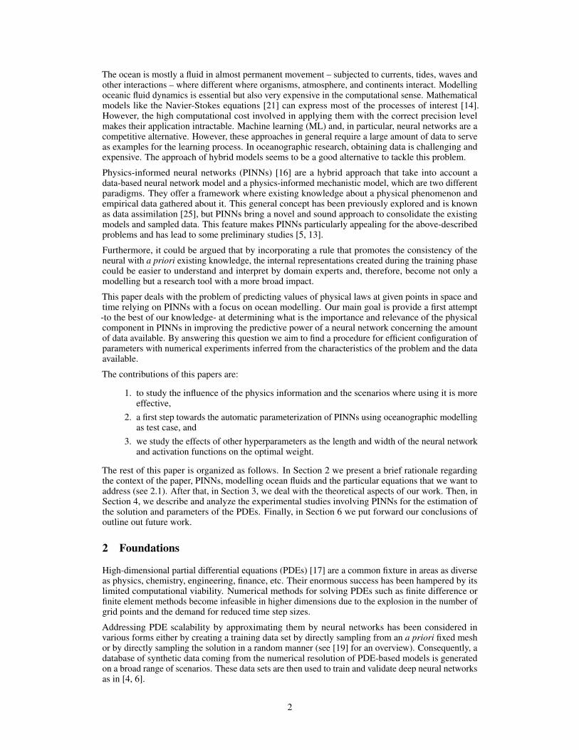
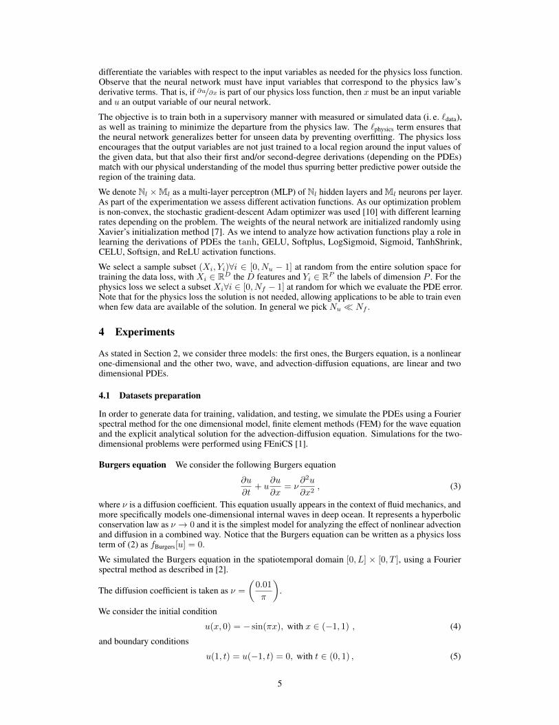
Figure 2: The relative error for different values of Nu and for different problems. Each dot representsthe final value of the relative error after training. We observe how the choice of λ affects trainingresults, and we observe a slight shift to higher λ values as Nu decreases. The dashed lines wereadded manually to aid in observing trends. For Burgers we note that the minimum shifts towards 1.0as Nu decreases, and for advection-diffusion the slope becomes more negative as Nu decreases. Thewave equation is more less evident, but it can be seen that for Nu = 500 and Nu = 200 the minimumlies around zero, while for Nu = 100 the trend has flattened and the results would be similar forλ ∈ [0.1, 0.9] roughly.

5 Results and discussion

See Table 1 for an overview of the used parameters for each of the models. The hyperparameters,such as the number and size of the hidden layers; the optimizer; and the number of epochs, werechosen either manually or by a grid search. All experiments were executed using Google Colab, aplatform to run notebooks on fast graphics processing units (GPUs). The ability of GPUs to runcalculations in parallel greatly enhances the speed of evaluating the neural network and calculatingthe gradients.1

1The data sets, source code, and results are available online at https://github.com/Inria-Chile/assessing-pinns-ocean-modelling and are released under the CeCILL license.

7

Table 1: Parameters for each of the models. Here epochs are the numbers of iterations over thetraining set, and Nu and Nf are the number of points used for the data loss and the physics lossrespectively. Nval

u is the number of data points used to for the validation data loss.

Model NN setup Optimizer Epochs Nu Nf Nvalu

Burgers 8× 20 Adam (lr=0.001) 25000 100, 200, 500 12800 25600Advec.-Diffusion 3× 40 Adam (lr=0.002) 20000 100, 500, 2500 5000 168100

Wave 5× 50 Adam (lr=0.001) 10000 100, 200, 500 10000 21800

Burgers AdvDif WavesModel

0.00

0.02

0.04

0.06

0.08

0.10

0.12

Rela

tive

erro

r

With physics lossWithout physics loss

(a) Errors with/without physics loss.

tanh GELU Softplus LogSigmoid Sigmoid TanhShrink CELU Softsign ReLUActivation function

10 2

10 1

Rela

tive

erro

r

BurgersAdvDifWaves

(b) Relative error using different activation functions.

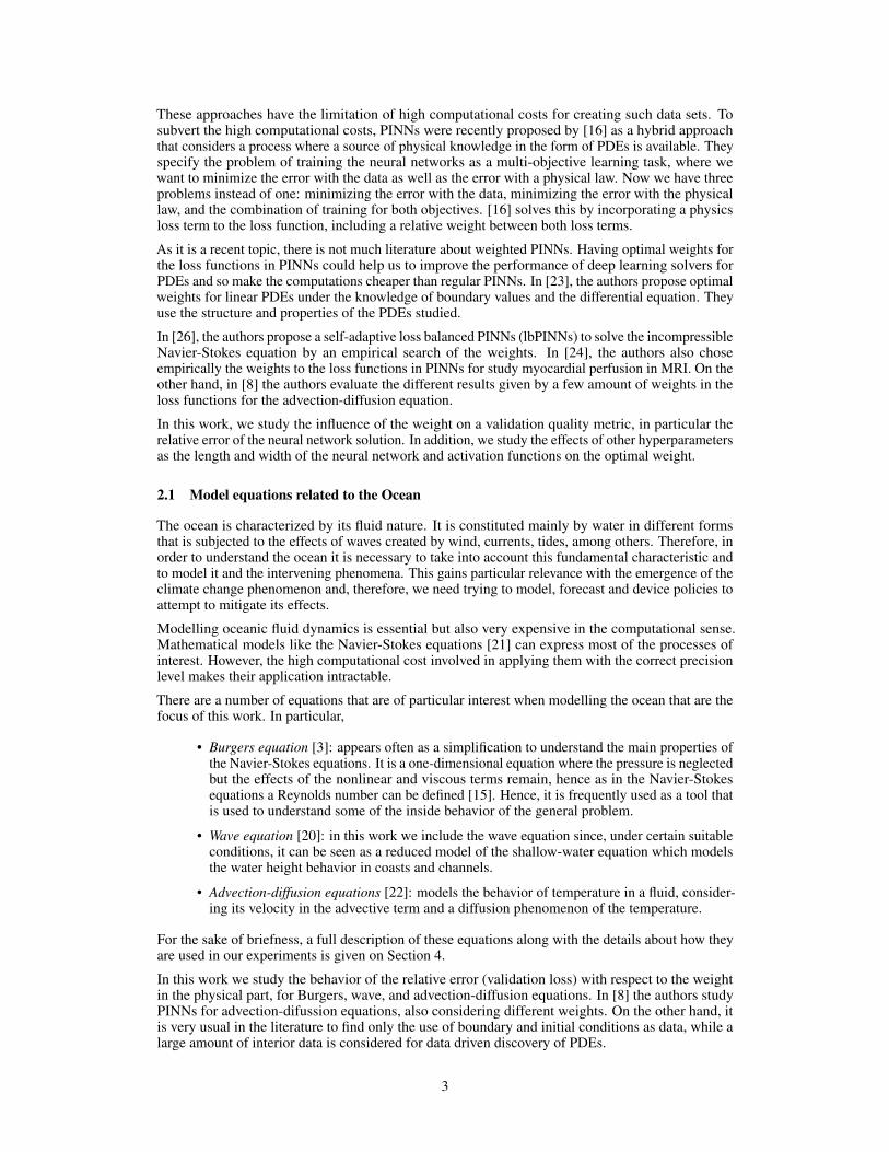
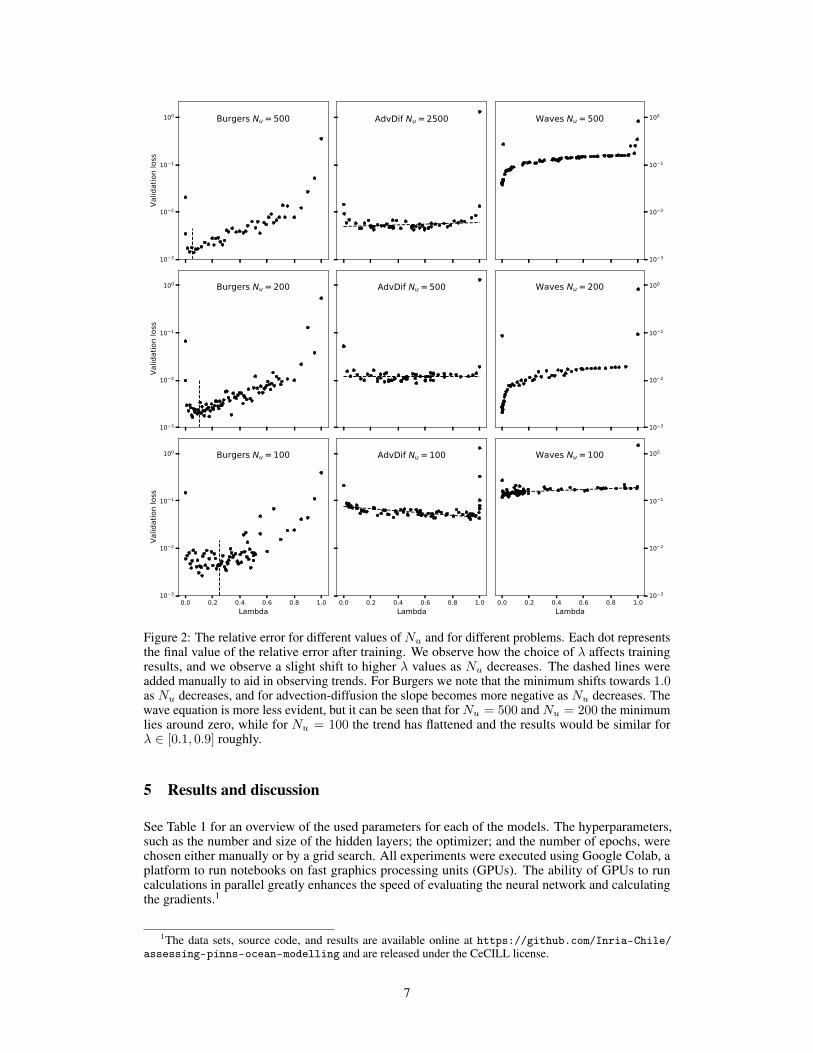
Figure 3: Summary of the experimental results. Fig. 3a shows results for 25 runs with and withoutphysics loss for each of the models. For Fig. 3b, Nu is 200, 500, and 200 and λ is 0.1, 0.5, and 0.002for the Burgers, advection-diffusion, and wave equations respectively.

To be able to compare the performance between models, the validation data loss is calculated overthe entire data set and then normalized as

Relative Error =

√MSE(Yval, Yval)

‖Yval‖2, (15)

where Yval are the labels of the validation data set, Yval the output of the neural network, and MSEthe mean squared error. In the case of advection-diffusion the labels Yi have been normalized to havezero mean and unit standard deviation to bring down the scale of the temperature, which is in Kelvin,to a range around zero. This obviates the need for the division when calculating the relative error.Additionally, to reduce the jitter in the loss while training, we use the lowest validation data loss ofthe last 250 epochs to calculate the relative error.

Learning the optimal value of λ, the relative weighting of the physics loss with respect to the dataloss is a metalearning objective in order to improve subsequent training of the same PINN. In Fig. 2we show the results of evaluating different problems using different values for Nu to find an optimalvalue of λ. A sharp rise in the relative error can be observed at λ = 0.0 and λ = 1.0, which areequivalent to training using solely the data loss or physics loss terms respectively. We note that theoptimal value for λ depends on the problem at hand and specifically on the scale of the data lossversus the physics loss. Normalizing the data set labels would in part solve the problem, but the scaleof the physics loss remains hard to normalize. In our experiments however, we note that for typicalvalues of λ the comparison of the data and physics loss remains roughly 0.1 < `data/`physics < 10.

Per problem we observe that at decreasing values for Nu, the optimal value of λ shifts slightlytowards 1.0. This trend suggests that as data become more sparse, the physics loss takes higherimportance. As less data are available, the information input from the physics loss helps trainingsignificantly, while the reverse holds as more data are available. At the limit where Nu is sufficientlylarge to be able to train the network autonomously, the optimal value of λ tends to zero.

In cases where few data points are known (i.e. Nu is small), the choice of the sample subset canhave a large influence on training results. In Fig. 3a the relative error is shown for 25 random datasubset selections with and without the physics loss. The added physics loss term reduces the relative

8

error, averaged over all three models, by 65% and reduces its standard deviation by 56%. PINNs thusimprove training results and reduce variability when the number of data points is low.

An analysis of how activation functions play a role in learning the derivations of PDEs, a comparisonis made with nine activation functions in Fig. 3b. Here we compare the tanh, GELU, Softplus,LogSigmoid, Sigmoid, TanhShrink, CELU, Softsign, ReLU activation function for their performance.It can be observed that especially the tanh and GELU activation functions and to a lesser extendSoftplus work well. The ReLU function produces poor results due to its inability to learn secondor higher derivatives. Due to the fact that a DNN using the ReLU activation function produces apiece-wise linear function [12], its second derivative is zero except at the points where the linearsegments meet, where it will be a Dirac function at x = 0, inhibiting learning second derivativesor higher. The Softsign and CELU functions have similar problems given their discontinuity of thesecond derivative at x = 0.

6 Final remarks

Information from the PDE serves in cases where data availability is limited to the extent that it wouldeither be unable to train the network satisfactorily using solely the data, or where results would varywidely depending on the selection of the data points. The addition of the physics loss term bothimproves training results and improves the stability of the training, even more so when the weight inthe loss function is optimal.

Finding the optimal weight of the loss function is a complex problem and this is, to the best of ourknowledge, the first study to understand the behavior of it with respect to different hyperparametersand PDEs. In the future, we expect to find the optimal weights using only the data available. Inaddition, it is also the first attempt at the study of PINNs for ocean modelling equations with verysimplified geometries. We expect to extend our results to more complex and realistic geometries inorder to use our results in real applications.

As λ has a dual role: the prior confidence in the training data vs. the PDE and the scaling of thesetwo terms, future work could understand each role of this parameter, which could be a possibleexplanation of why the optimal weight in some of our experiments are so different between differentmodels. In addition, as we observed for very small data sets, it would be interesting to find what“good” sample subsets of the problem for training are more stable under optimization. This would bethe first step to estimate the minimal amount of data required to train the neural networks in a robustway.

As the equations of interest are inherently wave-like, we propose to explore the benefits of Fouriertransformations for learning the equations more effectively, as was done by [11]. This would enablethe network to learn patterns of the data in the frequency space. Additionally, to generalize the modelbetter for unseen data, we propose the use of dropout by [9] to randomly turn off a percentage ofthe neurons. This forces the network to learn redundancies in case certain neurons are turned off,increasing the stability of the network, and the likelihood to generalize better for unseen data.

Future work on this topic is needed as it is required to develop better models for understanding theocean and integrate those models with others that explain the interaction between organisms and theenvironment. This is essential because of the constantly changing nature of the ocean.

We believe that PINNs have the potential of providing such tools, and therefore, serve as a buildingblock of a more comprehensive solution that addresses the ultimate issue of understanding andmitigating the climate change crisis. However, this potential also comes with important risks as usingan inadequate, biased, or non-transparent tool could lead instead to a deterioration. In this direction,as we already mentioned in the paper, we are interested in combining PINNs with explainable AI andpowerful visualization tools. Similarly, extended validation is necessary by domain experts.

Acknowledgments and Disclosure of Funding

This work is funded by project CORFO 10CEII-9157 Inria Chile and Inria Challenge project OcéanIA(desc. num 14500).

9

References[1] Alnæs, M. S., Blechta, J., Hake, J., Johansson, A., Kehlet, B., Logg, A., Richardson, C., Ring, J.,

Rognes, M. E., and Wells, G. N. (2015). The FEniCS project version 1.5. Archive of NumericalSoftware, 3(100).

[2] Basdevant, C., Deville, M., Haldenwang, P., Lacroix, J., Ouazzani, J., Peyret, R., Orlandi, P., andPatera, A. (1986). Spectral and finite difference solutions of the burgers equation. Computers &fluids, 14(1):23–41.

[3] Burgers, J. (1948). A mathematical model illustrating the theory of turbulence. In Von Mises, R.and Von Kármán, T., editors, Advances in Applied Mechanics, volume 1, pages 171–199. Elsevier.

[4] Chen, R. T., Rubanova, Y., Bettencourt, J., and Duvenaud, D. K. (2018). Neural ordinarydifferential equations. In Advances in neural information processing systems, pages 6571–6583.

[5] de Wolff, T., Carrillo Lincopi, H., Martí, L., and Sanchez-Pi, N. (2021). Assessing physicsinformed neural networks in ocean modelling and climate change applications. In Sanchez-Pi, N.and Martí, L., editors, AI: Modeling Oceans and Climate Change Workshop at ICLR 2021.

[6] Dupont, E., Doucet, A., and Teh, Y. W. (2019). Augmented neural ODEs. In Wallach, H.,Larochelle, H., Beygelzimer, A., d'Alché-Buc, F., Fox, E., and Garnett, R., editors, Advances inNeural Information Processing Systems 32, pages 3140–3150. Curran Associates, Inc.

[7] Glorot, X. and Bengio, Y. (2010). Understanding the difficulty of training deep feedforwardneural networks. In Teh, Y. W. and Titterington, M., editors, Proceedings of the ThirteenthInternational Conference on Artificial Intelligence and Statistics, volume 9 of Proceedings ofMachine Learning Research, pages 249–256, Chia Laguna Resort, Sardinia, Italy. PMLR.

[8] He, Q. and Tartakovsky, A. M. (2020). Physics-informed neural network method for forward andbackward advection-dispersion equations. arXiv preprint arXiv:2012.11658.

[9] Hinton, G. E., Srivastava, N., Krizhevsky, A., Sutskever, I., and Salakhutdinov, R. (2012).Improving neural networks by preventing co-adaptation of feature detectors. CoRR, abs/1207.0580.

[10] Kingma, D. P. and Ba, J. (2017). ADAM: A method for stochastic optimization.

[11] Li, Z., Kovachki, N., Azizzadenesheli, K., Liu, B., Bhattacharya, K., Stuart, A., and Anandku-mar, A. (2020). Fourier neural operator for parametric partial differential equations.

[12] Liu, B. and Liang, Y. (2021). Optimal function approximation with ReLU neural networks.Neurocomputing, 435:216–227.

[13] Lütjens, B., Crawford, C. H., Veillette, M., and Newman, D. (2021). PCE-PINNs: Physics-informed neural networks for uncertainty propagation in ocean modeling. In Sanchez-Pi, N. andMartí, L., editors, AI: Modeling Oceans and Climate Change Workshop at ICLR 2021.

[14] McLean, D. (2012). Understanding aerodynamics: arguing from the real physics. John Wiley& Sons.

[15] Orlandi, P. (2000). The Burgers equation, pages 40–50. Springer Netherlands, Dordrecht.

[16] Raissi, M., Perdikaris, P., and Karniadakis, G. (2019). Physics-informed neural networks: Adeep learning framework for solving forward and inverse problems involving nonlinear partialdifferential equations. Journal of Computational Physics, 378:686–707.

[17] Rao, K. S. (2010). Introduction to partial differential equations. PHI Learning Pvt. Ltd.

[18] Sánchez-Pi, N., Martí, L., Abreu, A., Bernard, O., de Vargas, C., Eveillard, D., Maass, A.,Marquet, P. A., Sainte-Marie, J., Salomon, J., Schoenauer, M., and Sebag, M. (2020). Artificialintelligence, machine learning and modeling for understanding the oceans and climate change.In Dao, D., Sherwin, E., Donti, P., Kaack, L., Kuntz, L., Yusuf, Y., Rolnick, D., Nakalembe,C., Monteleoni, C., and Bengio, Y., editors, Tackling Climate Change with Machine Learningworkshop at NeurIPS 2020.

10

[19] Sirignano, J. and Spiliopoulos, K. (2018). DGM: A deep learning algorithm for solving partialdifferential equations. Journal of Computational Physics, 375:339–1364.

[20] Stoker, J. J. (2011). Water waves: The mathematical theory with applications, volume 36. JohnWiley & Sons.

[21] Temam, R. (2001). Navier-Stokes equations: Theory and numerical analysis, volume 343.American Mathematical Soc.

[22] Union, J. I. G. (2013). Advection diffusion equation models in near-surface geophysical andenvironmental sciences. J. Ind. Geophys. Union (April 2013), 17(2):117–127.

[23] van der Meer, R., Oosterlee, C., and Borovykh, A. (2020). Optimally weighted loss functionsfor solving PDEs with neural networks. arXiv preprint arXiv:2002.06269.

[24] van Herten, R. L., Chiribiri, A., Breeuwer, M., Veta, M., and Scannell, C. M. (2020).Physics-informed neural networks for myocardial perfusion mri quantification. arXiv preprintarXiv:2011.12844.

[25] Vetra-Carvalho, S., van Leeuwen, P. J., Nerger, L., Barth, A., Altaf, M. U., Brasseur, P.,Kirchgessner, P., and Beckers, J.-M. (2018). State-of-the-art stochastic data assimilation methodsfor high-dimensional non-Gaussian problems. Tellus A: Dynamic Meteorology and Oceanography,70(1):1–43.

[26] Xiang, Z., Peng, W., Zheng, X., Zhao, X., and Yao, W. (2021). Self-adaptive loss balancedphysics-informed neural networks for the incompressible navier-stokes equations. arXiv preprintarXiv:2104.06217.

Checklist1. For all authors...

(a) Do the main claims made in the abstract and introduction accurately reflect the paper’scontributions and scope? [Yes]

(b) Did you describe the limitations of your work? [Yes](c) Did you discuss any potential negative societal impacts of your work? [Yes] See in

particular Section 6(d) Have you read the ethics review guidelines and ensured that your paper conforms to

them? [Yes]2. If you are including theoretical results...

(a) Did you state the full set of assumptions of all theoretical results? [Yes](b) Did you include complete proofs of all theoretical results? [N/A]

3. If you ran experiments...(a) Did you include the code, data, and instructions needed to reproduce the main experi-

mental results (either in the supplemental material or as a URL)? [Yes] See Section 5.(b) Did you specify all the training details (e.g., data splits, hyperparameters, how they

were chosen)? [Yes] See Section 5.(c) Did you report error bars (e.g., with respect to the random seed after running experi-

ments multiple times)? [Yes] See Section 5.(d) Did you include the total amount of compute and the type of resources used (e.g., type

of GPUs, internal cluster, or cloud provider)? [Yes] See Section 5.4. If you are using existing assets (e.g., code, data, models) or curating/releasing new assets...

(a) If your work uses existing assets, did you cite the creators? [N/A](b) Did you mention the license of the assets? [Yes] See Section 5.(c) Did you include any new assets either in the supplemental material or as a URL? [Yes]

See Section 5.(d) Did you discuss whether and how consent was obtained from people whose data you’re

using/curating? [N/A]

11

(e) Did you discuss whether the data you are using/curating contains personally identifiableinformation or offensive content? [N/A]

5. If you used crowdsourcing or conducted research with human subjects...(a) Did you include the full text of instructions given to participants and screenshots, if

applicable? [N/A](b) Did you describe any potential participant risks, with links to Institutional Review

Board (IRB) approvals, if applicable? [N/A](c) Did you include the estimated hourly wage paid to participants and the total amount

spent on participant compensation? [N/A]

12