Optimally Orienting Physical Networks

Optimally Orienting Physical Networks

*DANA SILVERBUSH,1 *MICHAEL ELBERFELD,2 and RODED SHARAN1

ABSTRACT

In a network orientation problem, one is given a mixed graph, consisting of directed andundirected edges, and a set of source-target vertex pairs. The goal is to orient the undirectededges so that a maximum number of pairs admit a directed path from the source to thetarget. This NP-complete problem arises in the context of analyzing physical networks ofprotein-protein and protein-DNA interactions. While the latter are naturally directed froma transcription factor to a gene, the direction of signal flow in protein-protein interactions isoften unknown or cannot be measured en masse. One then tries to infer this information byusing causality data on pairs of genes such that the perturbation of one gene changes theexpression level of the other gene. Here we provide a first polynomial-size ILP formulationfor this problem, which can be efficiently solved on current networks. We apply our algo-rithm to orient protein-protein interactions in yeast and measure our performance usingedges with known orientations. We find that our algorithm achieves high accuracy andcoverage in the orientation, outperforming simplified algorithmic variants that do not useinformation on edge directions. The obtained orientations can lead to a better understandingof the structure and function of the network.

Key words: integer linear program, mixed graph, network orientation, protein-DNA interaction,

protein-protein interaction.

1. INTRODUCTION

H igh-throughoutput technologies are routinely used nowadays to detect physical interac-

tions in the cell, including chromatin immuno-precipitation experiments for measuring protein-DNA

interactions (PDIs) (Lee et al., 2002), and yeast two-hybrid assays (Fields and Song, 1989) and co-

immunoprecipitation screens (Gavin et al., 2002) for measuring protein-protein interactions (PPIs). These

networks serve as the scaffold for signal processing in the cell and are, thus, key to understanding cellular

response to different genetic or environmental cues.

While PDIs are naturally directed (from a transcription factor to its regulated genes), PPIs are not.

Nevertheless, many PPIs transmit signals in a directional fashion, with kinase-substrate interactions (KPIs)

being one of the prime examples. These directions are vital to understanding signal flow in the cell, yet they

are not measured by most current techniques. Instead, one tries to infer these directions from perturbation

1Blavatnik School of Computer Science, Tel Aviv University, Tel Aviv, Israel.2Institute of Theoretical Computer Science, University of Lubeck, Lubeck, Germany.*These authors contributed equally to this work.

JOURNAL OF COMPUTATIONAL BIOLOGY

Volume 18, Number 11, 2011

# Mary Ann Liebert, Inc.

Pp. 1437–1448

DOI: 10.1089/cmb.2011.0163

1437

experiments. In these experiments, a gene (cause) is perturbed and as a result other genes change their

expression levels (effects). Assuming that each cause-effect pair should be connected by a directed pathway

in the physical network, one can predict an orientation (direction assignments) to the undirected part of the

network that will best agree with the cause-effect information.

The resulting combinatorial problem can be formalized by representing the network as a mixed graph,

where undirected edges model interactions with unknown causal direction, and directed edges represent

interactions with known directionality. The cause-effect pairs are modeled by a collection of source-target

vertex pairs. The goal is to orient (assign single directions to) the undirected edges so that a maximum

number of source-target pairs admit a directed path from the source to the target. We call this problem

MAXIMUM-MIXED-GRAPH-ORIENTATION.

Previous work on this and related problems can be classified into theoretical and applied work. On the

theoretical side, Arkin and Hassin (2002) studied the decision problem of orienting a mixed graph to admit

directed paths for a given set of source-target vertex pairs and showed that this problem is NP-complete.

The problem of finding strongly connected orientations of graphs can be solved in polynomial time (Boesch

and Tindell, 1980; Chung et al., 1985). Recently we proved that MAXIMUM-MIXED-GRAPH-OR-

IENTATION admits a sub-linear polynomial-time approximation (Elberfeld et al., 2011). For a compre-

hensive discussion of the various kinds of graph orientations, we refer to the textbook of Bang-Jensen and

Gutin (2008).

For the special case of an undirected network (with no pre-directed edges), the orientation problem was

shown to be NP-complete and hard to approximate to within a constant factor of 11/12 (Medvedovsky

et al., 2008). On the positive side, Medvedovsky et al. (2008) provided an ILP-based algorithm, and showed

that the problem is approximable to within a ratio of U(1/log n), where n is the number of vertices in the

network. The approximation ratio was later improved to U(log log n / log n) (Gamzu et al., 2010). Dorn

et al. (2011) studied the parameterized complexity of orienting undirected networks.

On the practical side, several authors studied the orientation problem and related annotation problems.

Yeang et al. (2004) were the first to use perturbation experiments to annotate protein networks. They

proposed a probabilistic model and an accompanying inference approach to predict edge directions and

signs of activation and repression from cause-effect data. Ourfali et al. (2007) provided an ILP formulation

for the problem of inferring edge signs that maximize the expected number of explained cause-effect pairs.

Gitter et al. (2011) used SATISFIABILITY-based approximations to tackle the orientation problem. The

main caveat of all these approaches is that they depend on enumerating all possible paths between a pair of

genes and, hence, they are limited to paths of very short length (3 for the first two works and 5 for the

latter).

Our main contribution in this article is a first efficient ILP formulation of the orientation problem on

mixed graphs, leading to an optimal solution of the problem on current networks. We implemented our

approach and applied it to a large data set of physical interactions and knockout pairs in yeast. We collected

interaction and cause-effect pair information from different publications and integrated them into a physical

network with 3,658 proteins, 2,639 PPIs, 4,095 PDIs, along with 53,809 knockout pairs among the mo-

lecular components of the network. We carried out a number of experiments to measure the accuracy of the

orientations produced by our method for different input scenarios. In particular, we studied how the portion

of undirected interactions and the number of cause-effect pairs affect the orientations. We further compared

our performance to that of two layman approaches that are based on orienting undirected networks,

ignoring the edge directionality information. We demonstrate that our method retains more information to

guide the search, achieving higher numbers of correctly oriented edges.

The article is organized as follows: In Section 2, we provide preliminaries and define the orientation

problem. In Section 3, we present an ILP-based algorithm to solve the orientation problem on mixed

graphs. In Section 4, we discuss our implementation of this algorithm, and in Section 5, we report on its

application to orient physical networks in yeast.

2. PRELIMINARIES

We focus on simple graphs with no loops or parallel edges. A mixed graph is a triple G = (V, EU, ED)

that consists of a set of vertices V, a set of undirected edges EU 4 {e 4 V r jej = 2}, and a set of directed

edges ED 4 V · V. We assume that every pair of vertices is either connected by a single edge of a specific

1438 SILVERBUSH ET AL.

type (directed or undirected) or not connected. For convenience, we also use the notations V(G), EU (G),

and ED (G) to refer to the sets V, EU, and ED, respectively. A mixed graph G is a directed graph if

EU (G) = ; (the empty set). It is an undirected graph if ED(G) = ;. A directed graph is strongly connected

if every vertex has a directed path to every other vertex.

Let G1 and G2 be two mixed graphs. The graph G1 is a subgraph of G2 if and only if the relations

V(G1) 4 V(G2), EU(G1) 4 EU(G2), and ED(G1) 4 ED(G2) hold; in this case we also write G1 4 G2. Si-

milarly, an induced subgraph G[V 0] is a subset V 04 V of the graph’s vertices and all their pairwise

relations (directed and undirected edges).

A path in a mixed graph G of length m is a sequence p¼ v1‚ v2‚ . . . ‚ vm‚ vmþ 1 of distinct vertices

vi 2 V(G) such that for every i 2 f1‚ . . . ‚ mg, we have fvi‚ viþ 1g 2 EU(G) or (vi‚ viþ 1) 2 ED(G). It is a

cycle if and only if v1 = vm + 1. A mixed graph with no cycles is called a mixed acyclic graph (MAG). Given

a pair of vertices s‚ t 2 V(G), we say that t is reachable from s if and only if there exists a path in G that goes

from s to t. We denote by C(G) the set of ordered pairs of vertices (s, t) such that t is reachable from s in G.

Let G be a mixed graph. An orientation of G is a directed graph G0 = (V(G),;,ED(G0)) over the same

vertex set whose edge set contains all the directed edges of G and a single directed instance of every

undirected edge, but nothing more. We are now ready to state the main optimization problem that we

tackle:

Problem 2.1 (MAXIMUM-MIXED-GRAPH-ORIENTATION).

Input: A mixed graph G, and a set of vertex pairs P 4 V(G) · V(G).

Output: An orientation G0 of G that satisfies a maximum number of pairs from P.

3. AN ILP ALGORITHM FOR ORIENTING MIXED GRAPHS

In this section, we present an integer linear program (ILP) for optimally orienting a mixed graph. The

inherent difficulty in developing such a program is that a direct approach, which represents every possible

path in the graph with a single variable (indicating whether, in a given orientation, this path exists or not),

leads to an exponential program. Below we will work toward a polynomial size program.

Many algorithms for problems on directed graphs first solve the problem for the graph’s strongly

connected components independently and, then, work along the directed acyclic graph (DAG) of strongly

connected components to produce a solution for the whole instance. Our ILP-based approach for orienting

mixed graphs has the same high level structure: In Section 3.1, we define a generalization of strongly

connected components to mixed graphs, called strongly orientable components, and show how the com-

putation of a solution for the orientation problem can be reduced to the mixed acyclic graph of strongly

orientable components. For MAGs, in turn, we present, in Section 3.2, a polynomial-size ILP that optimally

solves the orientation problem.

3.1. A reduction to a mixed acyclic graph

Let G be a mixed graph. The graph G is strongly orientable if and only if it can be oriented so that every

vertex is reachable from every other vertex (i.e., the resulting directed graph is strongly connected). The

strongly orientable components of G are its maximal strongly orientable subgraphs. It is straightforward to

prove that a graph can be partitioned into its strongly orientable components (by noting that if the vertex

sets of two strongly orientable graphs intersect, then their union is also strongly orientable). The strongly

orientable component graph, or component graph, GSOC of G is a mixed graph that is defined as follows: Its

vertices are the strongly orientable components C1‚ . . . ‚ Cn of G. Its edges are constructed as follows: For

every pair of distinct components Ci and Cj, there is a directed edge (Ci, Cj) in GSOC if and only if

(v‚ w) 2 ED(G) for some v 2 V(Ci) and w 2 V(Cj), and there is an undirected edge {Ci, Cj} in GSOC if and

only if fv‚ wg 2 EU(G) for some v 2 V(Ci) and w 2 V(Cj). Note that GSOC must be acyclic. The strongly

orientable components of a mixed graph G and, hence, the graph GSOC, can be computed in polynomial

time as follows: Repeatedly identify cycles in the graph and orient their undirected edges in a consistent

direction. After orienting all cycles the strongly connected components that are made up by the directed

edges are exactly the strongly orientable components of the initial graph.

OPTIMALLY ORIENTING PHYSICAL NETWORKS 1439

To complete the reduction we need to specify the new set of source-target pairs. This also involves a

slightly more general definition of the orientation problem where the collection of input pairs is allowed to

be a multi-set. Let P be the input multi-set for the original graph G. The multi-set PSOC for the reduced

graph is constructed as follows: for every pair (s‚ t) 2 P we insert a pair (C, C0) into PSOC, where C and C0

are the strongly orientable components that contain s and t, respectively. The following lemma establishes

the correctness for the reduction from instances (G, P) to (GSOC, PSOC).

Lemma 3.1. Let G be a mixed graph and P a set of vertex pairs from G. For every k 2 N there exists

an orientation G0 of G that satisfies k pairs from P if and only if there exists an orientation G0SOC of GSOC

that satisfies k pairs from PSOC.

Proof. For the ‘‘only if’’-direction, let G0 be an orientation of G that satisfies k pairs from P. Due to the

maximality of the components, there are no directed edges back and forth between different strongly

orientable components of G in G0. We can orient the edges of GSOC as follows: For every undirected edge

{Ci, Cj} of GSOC, we choose the orientation (Ci, Cj) if there exist vertices vi 2 Ci and vj 2 Cj with

(vi‚ vj) 2 ED(G0) and the orientation (Cj, Ci), otherwise. Let s and t be two vertices from G0 such that there

exists a path p from s to t in G0. The path p can be seen as an alternating sequence of (1) subpaths that lie

inside strongly orientable components of G and (2) edges that go from one strongly orientable component

to another. We build a path p0 out of the edges that connect components. The path p0 goes from Ci with

s 2 Ci to Cj with t 2 Cj.

For the ‘‘if’’-direction, we consider an orientation G0SOC of GSOC and extend it to an orientation G0 of G:

We choose a strongly connected orientation for every strongly orientable component of G and orient the

undirected edges between the components with respect to the orientation of the edges in GSOC. Since all

vertices in a strongly orientable component are reachable from each other we know that, whenever a pair

(Ci, Cj) is satisfied in G0SOC, then all pairs (s, t) with s 2 Ci and t 2 Cj are satisfied in G0. -

A mixed acyclic graph GSOC = (V, EU, ED) is, in general, neither a forest nor a directed acyclic graph. Its

structure inherits from both of these concepts: The undirected graph (V, EU, ;) is a forest whose trees are

connected by the directed edges ED without producing cycles. This observation gives rise to the following

definition of topological sortings for mixed graphs: A mixed graph G admits a topological sorting if (1) the

connected components of (V, EU, ;) are trees and (2) they can be arranged in a linear order T1‚ . . . ‚ Tn, such

that directed edges from ED can only go from a vertex in Ti to a vertex in Tj if i < j. Note that the definition

of topological sortings for MAGs also works for DAGs—with every tree being a single vertex. Moreover,

similar to DAGs, every MAG admits a topological sorting.

3.2. An ILP formulation for mixed acyclic graphs

Given an instance of a MAG G and a multiset of vertex pairs P, our ILP consists of a set of binary

orientation variables, describing the edge orientations, and binary closure variables, describing reachability

relations in the oriented graph. The objective of satisfying a maximum number of vertex pairs can then be

phrased as summing over closure variables for all pairs from P.

The ILP relies on a topological sorting T1‚ . . . ‚ Tn of the input MAG, which allows formulating con-

straints that force a consistent assignment of values to the orientation and closure variables. The formu-

lation is built iteratively on growing parts of the graph following the topological sorting. Specifically, for

every i 2 f1‚ . . . ‚ ng, we define Gi¼G[V(T1) [ � � � [ V(Ti)] and Pi = P X (V(Gi) · V(Gi)). Furthermore,

for every i 2 f2‚ . . . ‚ ng, we define Ei¼ED(G) \ (V(Gi� 1) · V(Ti)). The ILP I for G and P is made up by

the variable set variables(I) that is the union of the following binary variables:

o(v‚ w) j fv‚ wg 2 EU(G)� �

(1)

c(v‚ w) j (v‚ w) 2 V(G) · V(G)� �

(2)

fp(v‚ v0‚ w0‚ w) j 9 2pipn : (v‚ w) 2 V(Gi� 1) · V(Ti) ^ (v0‚ w0) 2 Eig (3)

The orientation variables in (1) are used to encode orientations of the edges: an assignment of 1 to o(v,w)

means that the undirected edge {v, w} is oriented from v to w. The closure variables in (2) are used to

represent which vertex pairs of the graph are satisfied: an assignment of 1 to c(v, w) will imply that there

exists a directed path from v to w in the orientation. During the construction we will set closure variables


c(v, w) with (v‚ w) 2 ED(G) to 1, and closure variables c(v, w) where w is not reachable from v to 0. Path

variables in (3) are used to describe the satisfaction of a vertex pair (v, w) by using an intermediate directed

edge (v0, w0): an assignment of 1 to p(v‚ v0‚ w0‚ w) will imply that there exists a directed path from v to w that

goes through the directed edge (v0, w0).The ILP contains the constraints

o(v‚ w)þ o(w‚ v)¼ 1 for all fv‚ wg 2 EU(G) (4)

c(v‚ w)po(x‚ y) for all v‚ w 2 V(Ti)‚ and all x‚ y 2 V(Ti)

where y comes directly after x on the

unique path from v to w in Ti‚ 1pipn (5)

c(v‚ w)p +(v0‚ w0)2Ei

p(v‚ v0‚ w0‚ w) for all (v‚ w) 2 V(Gi� 1) · V(Ti)‚ 2pipn (6)

p(v‚ v0‚ w0‚ w)pc(v‚ v0)‚ c(w0‚ w) for all(v‚ w) 2 V(Gi� 1) · V(Ti)‚ (v0‚ w0) 2 Ei‚ 2pipn (7)

and the objective

maximize +(s‚ t)2P

c(s‚ t) : (8)

Constraints in (4) force that each undirected edge is oriented in exactly one direction. The remaining

constraints in (5) to (7) are used to connect closure variables to the underlying orientation variables. They

force that a closure variable c(v, w) can only be set to 1 if the orientation variables describe a graph that

allows a directed path from v to w. Whenever v and w are in the same undirected component (which is a tree

since the whole graph is a MAG), they can only be connected via an orientation of the unique undirected

path between them. For vertex pairs of these kind constraint (5) ensures the above property. If v and w are

in different components Ti and Tj with i < j, we need to associate c(v, w) with all possible paths from v to w.

This is done by using the path variables: If there is a path from v to w, then it must visit a directed edge

(v0, w0) that starts in some component that precedes Tj and ends at T j (constraint (6)). Path variables are, in

turn, constrained by (7). The objective function maximizes the number of closure variables with assignment

1 that correspond to pairs from P. The following lemma formally establishes the correctness of the ILP.

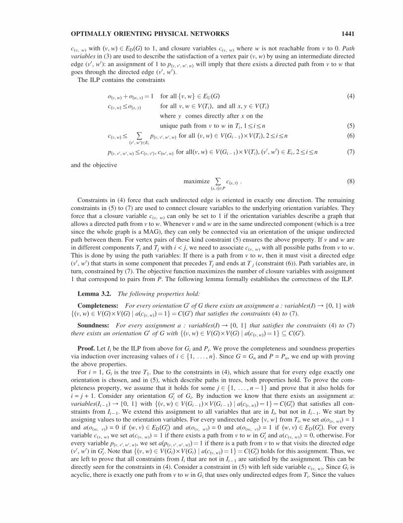
Lemma 3.2. The following properties hold:

Completeness: For every orientation G0 of G there exists an assignment a : variables(I) / {0, 1} with

f(v‚ w) 2 V(G) · V(G) j a(c(v‚ w))¼ 1g¼C(G0) that satisfies the constraints (4) to (7).

Soundness: For every assignment a : variables(I) / {0, 1} that satisfies the constraints (4) to (7)

there exists an orientation G0 of G with f(v‚ w) 2 V(G) · V(G) j a(c(v‚ w))¼ 1g � C(G0).

Proof. Let Ii be the ILP from above for Gi and Pi. We prove the completeness and soundness properties

via induction over increasing values of i 2 f1‚ . . . ‚ ng. Since G = Gn and P = Pn, we end up with proving

the above properties.

For i = 1, Gi is the tree T1. Due to the constraints in (4), which assure that for every edge exactly one

orientation is chosen, and in (5), which describe paths in trees, both properties hold. To prove the com-

pleteness property, we assume that it holds for some j 2 f1‚ . . . ‚ n� 1g and prove that it also holds for

i = j + 1. Consider any orientation G0i of Gi. By induction we know that there exists an assignment a:

variables(Ii - 1) / {0, 1} with f(v‚ w) 2 V(Gi� 1) · V(Gi� 1) j a(c(v‚ w))¼ 1g¼C(G0i) that satisfies all con-

straints from Ii - 1. We extend this assignment to all variables that are in Ii, but not in Ii - 1. We start by

assigning values to the orientation variables. For every undirected edge {v, w} from Ti, we set a(o(v, w)) = 1

and a(o(w, v)) = 0 if (w‚ v) 2 ED(G0i) and a(o(v, w)) = 0 and a(o(w, v)) = 1 if (w‚ v) 2 ED(G0i). For every

variable c(v, w) we set a(c(v, w)) = 1 if there exists a path from v to w in G0i and a(c(v, w)) = 0, otherwise. For

every variable p(v‚ v0‚ w0‚ w), we set a(p(v‚ v0‚ w0‚ w))¼ 1 if there is a path from v to w that visits the directed edge

(v0, w0) in G0i. Note that f(v‚ w) 2 V(Gi) · V(Gi) j a(c(v‚ w))¼ 1g¼C(G0i) holds for this assignment. Thus, we

are left to prove that all constraints from Ii that are not in Ii - 1 are satisfied by the assignment. This can be

directly seen for the constraints in (4). Consider a constraint in (5) with left side variable c(v, w). Since Gi is

acyclic, there is exactly one path from v to w in Gi that uses only undirected edges from Ti. Since the values


of the orientation variables correspond to the orientation of edges in G0i, the constraint is satisfied. Consider

a constraint in (6) with left side variable c(v, w). If a(c(v, w)) = 1, then there exists a path from the vertex

v 2 V(Gi� 1) to the vertex w 2 V(Ti) via some edge (v0, w0) with v0 2 V(Gi� 1) and w0 2 V(Ti). We assigned

the value 1 to the corresponding variable p(v‚ v0‚ w0‚ w). Thus, the constraint is satisfied. For a constraint in (7),

let p(v‚ v0‚ w0‚ w) be the left side variable of the inequations. If a(p(v‚ v0‚ w0‚ w))¼ 1, then there is a path from v to w

via the directed edge (v0, w0). By the induction hypothesis we know that a(c(v‚ v0))¼ 1 and, by our assignment

we know that a(c(w0‚ w))¼ 1. Thus, the constraint is satisfied.

To prove the induction step for the soundness property, let a : variables(Ii) / {0, 1} be an assignment

that satisfies all constraints from Ii. By the induction hypothesis, there exists an orientation G0i� 1 of Gi - 1

with f(v‚ w) 2 V(Gi� 1) · V(Gi� 1) j a(c(v‚ w))¼ 1g � C(G0i� 1). We extend this orientation to an orientation

G0i for Gi by orienting the edges {v, w} of Ti: If a(o(v, w)) = 1, we choose the orientation (v, w); otherwise,

we choose (w, v). We now prove that for every variable c(v, w) with a(c(v, w)) = 1, there exists a path from v

to w in G0i. The induction hypothesis implies that this holds if v‚ w 2 V(Gi� 1). We prove that this also holds

for all other vertex pairs: If v‚ w 2 Ti, the constraint in (5) with left side variable c(v, w) witnesses that there

exists a path from v to w through vertices from Ti. If (v‚ w) 2 V(Gi� 1) · V(Ti), the constraint in (6) with left

side variable c(c,w) witnesses that, for some directed edge (v0,w0) from Gi - 1 to Ti, we have a(p(v‚ v0‚ w0‚ w))¼ 1.

The constraint in (7) of p(v‚ v0‚ w0‚ w), in turn, witnesses that a(c(v‚ v0))¼ 1 and a(c(w0‚ w))¼ 1. By the induction

hypothesis, we know that there is a path from v to v0 in G0i, and as argued above, there is also a path from w0

to w in Ti. Together with the directed edge from v0 to w0, we conclude that there is a path from v to w in

G0i. -

The ILP has polynomial size and can be constructed in polynomial time. The construction starts by

sorting the MAG topologically. Constant length constraints in (4) are constructed for all undirected edges.

For every ordered pair (v, w) of vertices v and w that are inside the same undirected component Ti, we

construct at most jEUj constraints of type (5) using reachability queries to Ti. The sum constraints in (6) are

constructed for all ordered vertex pairs (v, w) where the undirected component of v comes before the

undirected component of w in the topological sorting of the MAG. Each sum iterates over the directed

edges that lead into the component of w. Thus, each sum’s length is bounded by O(jEDj) and it can be

written down in polynomial time. The constraints in (7) of constant length are constructed by iterating over

the same vertex pairs and directed edges. In total, the size of the ILP is at most O(jV(G)j2(jEDj + jEUj)).One may ask if it is possible to apply the ILP construction to general mixed graphs instead of MAGs. The

MAG-based construction explores a mixed acyclic graph G iteratively by using a topological sorting

T1‚ . . . ‚ Tn for it. It relies on the fact that the Ti’s are trees (which means that there is exactly one path

between any two vertices from the same tree Ti) and that directed edges can only go from a tree Ti to a tree

Tj if i < j. In a mixed cyclic graph, the undirected components are not necessarily trees and there may be

directed edges going back and forth between them. This prevents the iterative construction and implies a

construction that needs to revise already constructed parts of the formulation instead of just appending new

constraints at each step. We are not aware of any method that directly produces polynomial size ILP

formulations for general graphs.

4. IMPLEMENTATION DETAILS

Our implementation is written in C + + using BOOST C + + libraries (version number 1.43.0) and the

commercial IBM ILOG CPLEX optimizer (version number 12) to solve ILPs. The input of our program

consists of a mixed graph G = (V, EU, ED) and a collection P of vertex pairs from G. The program predicts

an orientation G0 for G that satisfies a maximum number of pairs from P.

The program starts by computing strongly connected orientations for all strongly orientable components

of the input graph. This can be done in polynomial time, as described in Section 3.1. Our program

implements a linear time approach for this step that is based on combined ideas from Tarjan (1972) and

Chung et al. (1985). Next, the program computes the acyclic component graph GSOC of G and transforms

the collection of pairs P into the collection of pairs PSOC. Finally, the program computes an optimal

orientation for the resulting instance (GSOC, PSOC) via the ILP approach from Section 3.2. This results in an

orientation for all undirected edges that are not inside strongly orientable components and the number of

satisfied pairs, which is optimal. Altogether, the program outputs an optimal orientation for the input


instance and, if desired, the satisfied pairs and their number. The resulting computational pipeline is shown

in Figure 1, and an example of it is provided in Figure 2.

Due to the combinatorial nature of our approach, there is possibly more than one orientation that results

in an optimal number of satisfied pairs. To determine if an undirected edge e = {v, w} has the same

orientation in all maximum solutions, one can utilize our computational pipeline as follows: First compute

the number sOPT of satisfied pairs in an optimal solution. Let (v, w) be the orientation of e in this solution.

Then run the experiment again, but this time with {v, w} replaced by the directed edge (w, v) in the input

network. After that set a confidence value ce = sOPT - se, where se is the maximum number of satisfied

pairs for the modified instance. The edge e is said to be oriented with confidence if and only if ce ‡ 1; in this

case its direction is the same in all optimal orientations of the input.

5. EXPERIMENTAL RESULTS

5.1. Data acquisition and integration

We gathered protein-protein interactions and cause-effect pair information for Saccharomyces cerevisiae

from different sources. We used the protein-protein interaction (PPI) data set ‘‘Y2H-union’’ from Yu et al.

(2008), which contains 2,930 highly-reliable undirected interactions between 2,018 proteins. The protein-

DNA interaction (PDI) data were taken from MacIsaac et al. (2006), an update of which can be found at

http://fraenkel.mit.edu/improved_map/. We used the collection of PDIs with

p < 0.001 conserved over at least two other yeast species, which consists of 4,113 unique PDIs spanning

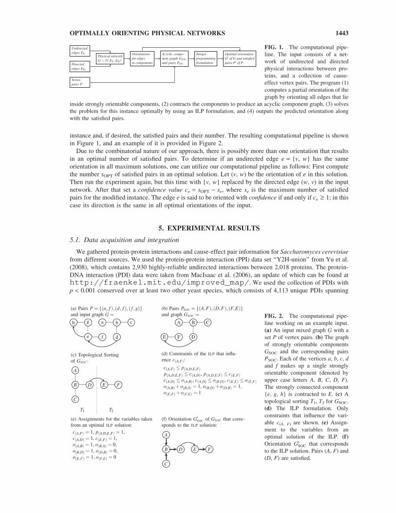
FIG. 1. The computational pipe-

line. The input consists of a net-

work of undirected and directed

physical interactions between pro-

teins, and a collection of cause-

effect vertex pairs. The program (1)

computes a partial orientation of the

graph by orienting all edges that lie

inside strongly orientable components, (2) contracts the components to produce an acyclic component graph, (3) solves

the problem for this instance optimally by using an ILP formulation, and (4) outputs the predicted orientation along

with the satisfied pairs.

FIG. 2. The computational pipe-

line working on an example input.

(a) An input mixed graph G with a

set P of vertex pairs. (b) The graph

of strongly orientable components

GSOC and the corresponding pairs

PSOC. Each of the vertices a, b, c, d

and f makes up a single strongly

orientable component (denoted by

upper case letters A, B, C, D, F).

The strongly connected component

{e, g, h} is contracted to E. (c) A

topological sorting T1, T2 for GSOC.

(d) The ILP formulation. Only

constraints that influence the vari-

able c(A, F) are shown. (e) Assign-

ment to the variables from an

optimal solution of the ILP. (f)

Orientation G0SOC that corresponds

to the ILP solution. Pairs (A, F) and

(D, F) are satisfied.


2,079 proteins. The kinase-substrate interactions (KPIs) were collected from Breitkreutz et al. (2010) by

taking the directed kinase-substrate interactions out of their data set. This results in 1,361 KPIs among 802

proteins. A set of 110,487 knockout pairs among 6,228 proteins were taken from Reimand et al. (2010).

We integrated the data to obtain a physical network of undirected and directed interactions. We removed

self loops and parallel interactions; for the latter, whenever both a directed and an undirected edge were

present between the same pair of vertices, we maintained the former only. Pairs of edges that are directed in

opposite directions were maintained, and will be contracted into single vertices in later phases of the

preprocessing. The resulting physical network, which we call the integrated network, spans 3,658 proteins,

2,639 PPIs, 4,095 PDIs, and 1,361 KPIs. For some of the following experiments, we wish to investigate the

contribution of the directed edges to the orientation in a purified manner. To this end, we will also use the

subnetwork of 2,579 proteins of the integrated network that is obtained by taking only the directed PDIs

and PKIs, leaving the PPIs out; we call it the refined network. To orient the physical networks, we use the

set of 110,487 knockout pairs and consider the subset of pairs with endpoints being in the physical network.

The integrated network contains 53,809 of the pairs; the refined network contains 34,372 of the pairs.

5.2. Application and performance evaluation

To study the behavior and properties of our algorithm, we apply it to the physical networks and monitor

properties of the instance from the intermediate steps and the resulting orientations. For the former, we

examine the contraction step, monitoring the size of the component graph obtained (numbers of vertices,

directed edges, and undirected edges), and the number of cause-effect pairs after the contraction. For the

latter, we run the algorithm in a cross-validation setting, hiding the directions of some of the edges and

testing our success in orienting them.

The component graph for the integrated network contains 763 undirected edges and 2,910 directed edges

among 2,569 vertices. We filter from the corresponding set of pairs PSOC those pairs that have the same

source and target vertices; these pairs lie inside strongly orientable components and are already satisfied.

About 85% (44,825) of the initial pairs remain in the contracted graph and can be used to guide the

orientation produced by our ILP.

Measuring runtime. The algorithm is relatively fast and, depending on the input instance, computes

an orientation in about a minute. In detail, on the integrated network, the preprocessing step takes 3 seconds

and the solution of the ILP takes 70 seconds. Considering only the refined network, the preprocessing takes

5 seconds, as there are eventually more components in the contracted graph, and the ILP is solved in 57

seconds, as there are less choices to be made.

Investigating the runtime further, we found that while the preprocessing time is approximately constant

(a few seconds), the ILP solution time is variable. It is influenced by a number of factors, among which are

the amount of undirected edges to which the solver assigns a direction, and the number of undirected

components in the contracted graph, which directly influences the number of constraints in the ILP. The

dominant factor was the number of pairs that have a source to target path, which constitutes the objective of

the program.

The computational intensive part is the computation of confidence scores. These entail rerunning the

steps of the computational pipeline for each of the oriented edges, resulting in about 3.4 hours for the

integrated network and 5 hours for the refined network (in which more test edges remain after the cycle

contraction).

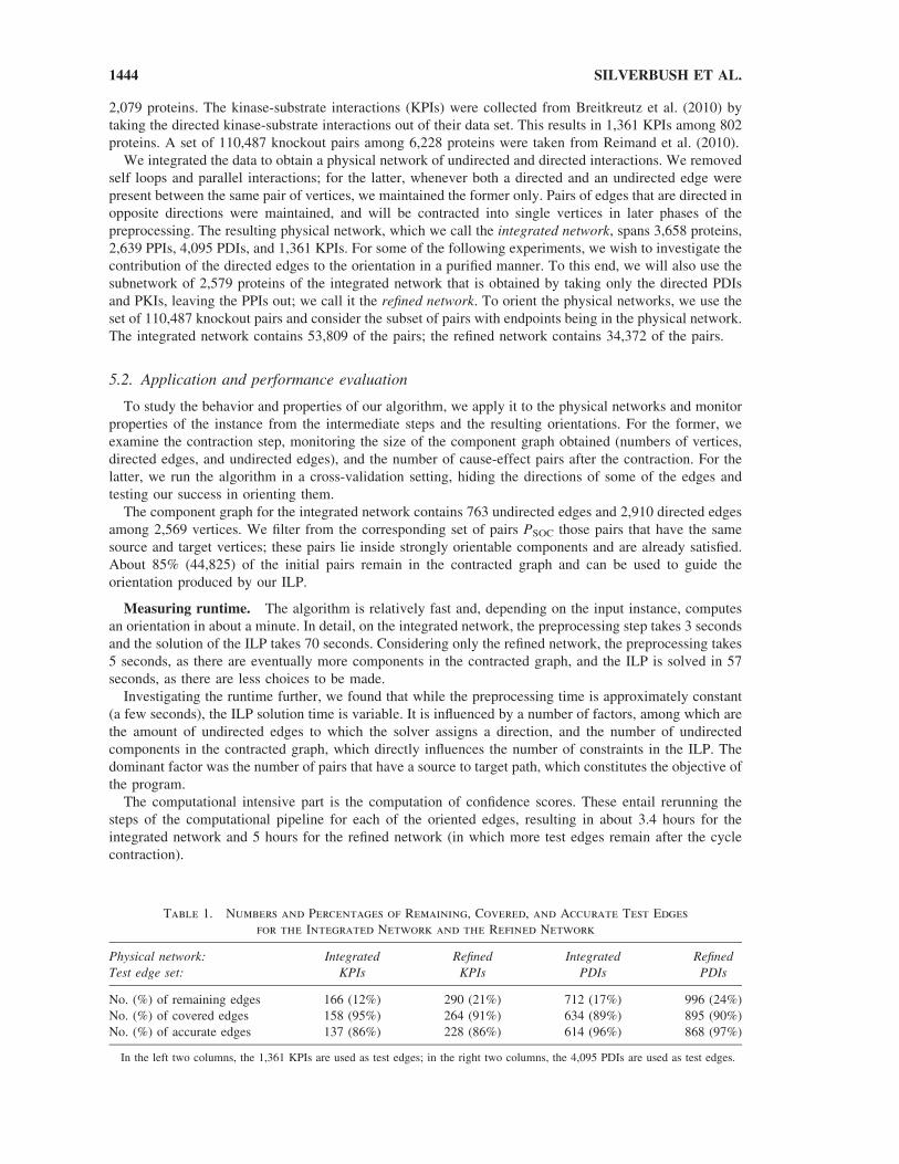
Table 1. Numbers and Percentages of Remaining, Covered, and Accurate Test Edges

for the Integrated Network and the Refined Network

Physical network: Integrated Refined Integrated Refined

Test edge set: KPIs KPIs PDIs PDIs

No. (%) of remaining edges 166 (12%) 290 (21%) 712 (17%) 996 (24%)

No. (%) of covered edges 158 (95%) 264 (91%) 634 (89%) 895 (90%)

No. (%) of accurate edges 137 (86%) 228 (86%) 614 (96%) 868 (97%)

In the left two columns, the 1,361 KPIs are used as test edges; in the right two columns, the 4,095 PDIs are used as test edges.


Measuring accuracy and coverage. To evaluate the orientations suggested by our algorithm, we

defined a subset of the directed edges in the input graph (KPIs or PDIs) as undirected test edges. Guided by

the set of knockout pairs, our program computes orientations for all undirected edges, including the test edges.

In the evaluation of the orientation, we focus on test edges that survive the contraction and remain in the

component graph, as the orientation of the other test edges depends only on the cycles they lie in and not on

the input cause-effect pairs. We further focus on confident orientations, as other orientations are arbitrary. We

define the coverage of an orientation as the percent of remaining test edges that are oriented with confidence.

The accuracy of an orientation is the percent of confidently oriented test edges whose orientation is correct.

Table 1 shows the number of remaining, covered, and accurate test edges for the integrated network and the

refined network where either the KPIs or the PDIs are used as test edges. Expectedly, more test edges remain

in the refined network; coverage and accuracy are high in all experiments.

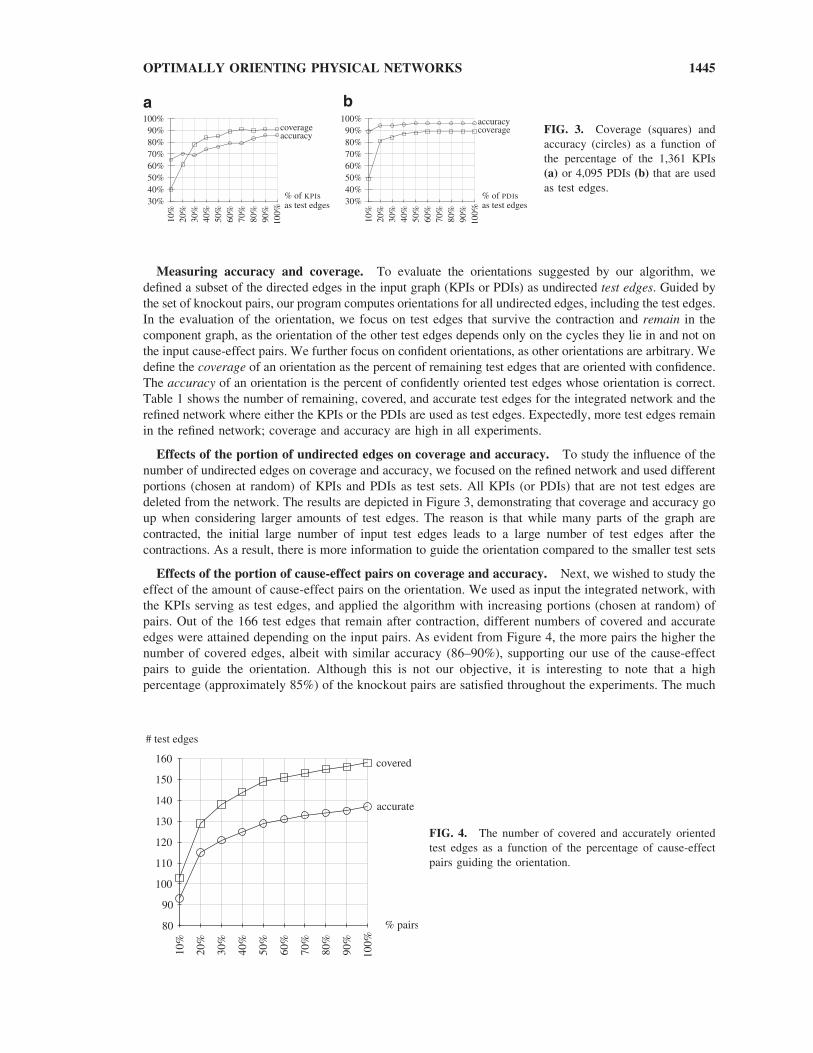
Effects of the portion of undirected edges on coverage and accuracy. To study the influence of the

number of undirected edges on coverage and accuracy, we focused on the refined network and used different

portions (chosen at random) of KPIs and PDIs as test sets. All KPIs (or PDIs) that are not test edges are

deleted from the network. The results are depicted in Figure 3, demonstrating that coverage and accuracy go

up when considering larger amounts of test edges. The reason is that while many parts of the graph are

contracted, the initial large number of input test edges leads to a large number of test edges after the

contractions. As a result, there is more information to guide the orientation compared to the smaller test sets

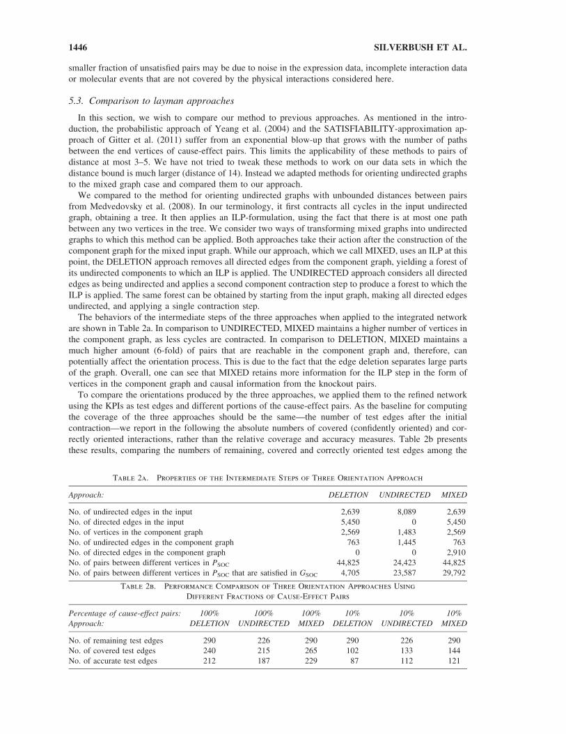
Effects of the portion of cause-effect pairs on coverage and accuracy. Next, we wished to study the

effect of the amount of cause-effect pairs on the orientation. We used as input the integrated network, with

the KPIs serving as test edges, and applied the algorithm with increasing portions (chosen at random) of

pairs. Out of the 166 test edges that remain after contraction, different numbers of covered and accurate

edges were attained depending on the input pairs. As evident from Figure 4, the more pairs the higher the

number of covered edges, albeit with similar accuracy (86–90%), supporting our use of the cause-effect

pairs to guide the orientation. Although this is not our objective, it is interesting to note that a high

percentage (approximately 85%) of the knockout pairs are satisfied throughout the experiments. The much

ba

FIG. 3. Coverage (squares) and

accuracy (circles) as a function of

the percentage of the 1,361 KPIs

(a) or 4,095 PDIs (b) that are used

as test edges.

FIG. 4. The number of covered and accurately oriented

test edges as a function of the percentage of cause-effect

pairs guiding the orientation.


smaller fraction of unsatisfied pairs may be due to noise in the expression data, incomplete interaction data

or molecular events that are not covered by the physical interactions considered here.

5.3. Comparison to layman approaches

In this section, we wish to compare our method to previous approaches. As mentioned in the intro-

duction, the probabilistic approach of Yeang et al. (2004) and the SATISFIABILITY-approximation ap-

proach of Gitter et al. (2011) suffer from an exponential blow-up that grows with the number of paths

between the end vertices of cause-effect pairs. This limits the applicability of these methods to pairs of

distance at most 3–5. We have not tried to tweak these methods to work on our data sets in which the

distance bound is much larger (distance of 14). Instead we adapted methods for orienting undirected graphs

to the mixed graph case and compared them to our approach.

We compared to the method for orienting undirected graphs with unbounded distances between pairs

from Medvedovsky et al. (2008). In our terminology, it first contracts all cycles in the input undirected

graph, obtaining a tree. It then applies an ILP-formulation, using the fact that there is at most one path

between any two vertices in the tree. We consider two ways of transforming mixed graphs into undirected

graphs to which this method can be applied. Both approaches take their action after the construction of the

component graph for the mixed input graph. While our approach, which we call MIXED, uses an ILP at this

point, the DELETION approach removes all directed edges from the component graph, yielding a forest of

its undirected components to which an ILP is applied. The UNDIRECTED approach considers all directed

edges as being undirected and applies a second component contraction step to produce a forest to which the

ILP is applied. The same forest can be obtained by starting from the input graph, making all directed edges

undirected, and applying a single contraction step.

The behaviors of the intermediate steps of the three approaches when applied to the integrated network

are shown in Table 2a. In comparison to UNDIRECTED, MIXED maintains a higher number of vertices in

the component graph, as less cycles are contracted. In comparison to DELETION, MIXED maintains a

much higher amount (6-fold) of pairs that are reachable in the component graph and, therefore, can

potentially affect the orientation process. This is due to the fact that the edge deletion separates large parts

of the graph. Overall, one can see that MIXED retains more information for the ILP step in the form of

vertices in the component graph and causal information from the knockout pairs.

To compare the orientations produced by the three approaches, we applied them to the refined network

using the KPIs as test edges and different portions of the cause-effect pairs. As the baseline for computing

the coverage of the three approaches should be the same—the number of test edges after the initial

contraction—we report in the following the absolute numbers of covered (confidently oriented) and cor-

rectly oriented interactions, rather than the relative coverage and accuracy measures. Table 2b presents

these results, comparing the numbers of remaining, covered and correctly oriented test edges among the

Table 2a. Properties of the Intermediate Steps of Three Orientation Approach

Approach: DELETION UNDIRECTED MIXED

No. of undirected edges in the input 2,639 8,089 2,639

No. of directed edges in the input 5,450 0 5,450

No. of vertices in the component graph 2,569 1,483 2,569

No. of undirected edges in the component graph 763 1,445 763

No. of directed edges in the component graph 0 0 2,910

No. of pairs between different vertices in PSOC 44,825 24,423 44,825

No. of pairs between different vertices in PSOC that are satisfied in GSOC 4,705 23,587 29,792

Table 2b. Performance Comparison of Three Orientation Approaches Using

Different Fractions of Cause-Effect Pairs

Percentage of cause-effect pairs: 100% 100% 100% 10% 10% 10%

Approach: DELETION UNDIRECTED MIXED DELETION UNDIRECTED MIXED

No. of remaining test edges 290 226 290 290 226 290

No. of covered test edges 240 215 265 102 133 144

No. of accurate test edges 212 187 229 87 112 121


three approaches. Evidently, MIXED yields higher numbers of test edges, covered edges, and correctly

oriented edges. The differences between DELETION and MIXED are more pronounced when the input set

of cause-effect pairs is smaller. This nicely corresponds to the dramatic difference between the numbers of

pairs that are reachable in the corresponding component graphs.

6. CONCLUSION

We presented an ILP algorithm that efficiently computes optimal orientations for mixed graph inputs.

We implemented the method and applied it to the orientation of physical interaction networks in yeast.

Depending on the input, the method yields very high coverage and accuracy in the orientation. Our

experiments further show that the algorithm works very fast in practice and produces orientations that cover

(accurately) larger portions of the network compared to the ones produced by previous approaches that

ignore the directionality information and operate on undirected versions of the networks. Nevertheless, all

these methods suffer from the ambiguity of direction assignment to edges on cycles; as a result, only 12–

22% of the undirected edges in the network are confidently oriented in our experiments.

While in this article we concentrated on the computational challenges in network orientation, the use of

the obtained orientations to gain biological insights on the pertaining networks is of great importance. As

demonstrated by Gitter et al. (2011), the directionality information facilitates pathway inference. It may

also contribute to module detection; in particular, it is intriguing in this context to map the correspondence

between contracted edges (under our method) and known protein complexes.

ACKNOWLEDGMENTS

A preliminary version of this paper was presented at RECOMB 2011 (Silverbush et al., 2011). M.E. was

supported by a research grant from the Dr. Alexander und Rita Besser-Stiftung. R.S. was supported by a

research grant from the Israel Science Foundation (grant 385/06).

DISCLOSURE STATEMENT

No competing financial interests exist.

REFERENCES

Arkin, E.M., and Hassin, R. 2002. A note on orientations of mixed graphs. Discrete Appl. Math. 116, 271–278.

Bang-Jensen, J., and Gutin, G. 2008. Digraphs: Theory, Algorithms and Applications, 2nd ed. Springer, New York.

Boesch, F., and Tindell, R. 1980. Robbins’s theorem for mixed multigraphs. Am. Math. Monthly 87, 716–719.

Breitkreutz, A., Choi, H., Sharom, J.R., et al. 2010. A global protein kinase and phosphatase interaction network in

yeast. Science 328, 1043–1046.

Chung, F.R.K., Garey, M.R., and Tarjan, R.E. 1985. Strongly connected orientations of mixed multigraphs. Networks

15, 477–484.

Dorn, B., Huffner, F., Kruger, D., et al. 2011. Exploiting bounded signal flow for graph orientation based on cause-

effect pairs. Lect. Notes Comput. Sci. 6595, 104–115.

Elberfeld, M., Segev, D., Davidson, C.R., et al. 2011. Approximation algorithms for orienting mixed graphs. Lect.

Notes Comput. Sci. 6661.

Fields, S., and Song, O. 1989. A novel genetic system to detect protein-protein interactions. Nature 340, 245–246.

Gamzu, I., Segev, D., and Sharan, R. 2010. Improved orientations of physical networks. Lect. Notes Comput. Sci. 6293,

215–225.

Gavin, A., Bosche, M., Krause, R., et al. 2002. Functional organization of the yeast proteome by systematic analysis of

protein complexes. Nature 415, 141–147.

Gitter, A., Klein-Seetharaman, J., Gupta, A., et al. 2011. Discovering pathways by orienting edges in protein interaction

networks. Nucleic Acids Res. 39, e22.

Lee, T.I., Rinaldi, N.J., Robert, F., et al. 2002. Transcriptional regulatory networks in Saccharomyces cerevisiae.

Science 298, 799–804.


MacIsaac, K., Wang, T., Gordon, D.B., et al. 2006. An improved map of conserved regulatory sites for Saccharomyces

cerevisiae. BMC Bioinform. 7, 113.

Medvedovsky, A., Bafna, V., Zwick, U., et al. 2008. An algorithm for orienting graphs based on cause-effect pairs and

its applications to orienting protein networks. Lect. Notes Comput. Sci. 5251, 222–232.

Ourfali, O., Shlomi, T., Ideker, T., et al. 2007. SPINE: a framework for signaling-regulatory pathway inference from

cause-effect experiments. Bioinformatics 23, i359–i366.

Reimand, J., Vaquerizas, J.M., Todd, A.E., et al. 2010. Comprehensive reanalysis of transcription factor knockout

expression data in Saccharomyces cerevisiae reveals many new targets. Nucleic Acids Res. 38, 4768–4777.

Silverbush, D., Elberfeld, M., and Sharan, R. 2011. Optimally orienting physical networks. Lect. Notes Comput. Sci.

6577, 424–436.

Tarjan, R. 1972. Depth-first search and linear graph algorithms. SIAM J. Comput. 1, 146–160.

Yeang, C., Ideker, T., and Jaakkola, T. 2004. Physical network models. J. Comput. Biol. 11, 243–262.

Yu, H., Braun, P., Yildirim, M.A., et al. 2008. High-quality binary protein interaction map of the yeast interactome

network. Science 322, 104–110.

Address correspondence to:

Dr. Roded Sharan

Blavatnik School of Computer Science

Tel Aviv University

Tel Aviv 69978, Israel

E-mail: [email protected]


Optimally Orienting Physical Networks

Documents

Transcript of Optimally Orienting Physical Networks