Final Report

Title: Investigation of Unsteady Flow Physics around Blunt

Shaped MAV using CFD

AFOSR/AOARD Reference Number: AOARD-09-4097

AFOSR/AOARD Program Manager: John Seo, Lt Col, USAF, Ph.D.

Period of Performance: JUL09 – JUL10

Submission Date: 24 September 2010

PI: Moon-Sang Kim, Korea Aerospace University, Goyang, 412-791, KOREA

Report Documentation Page Form ApprovedOMB No. 0704-0188

Public reporting burden for the collection of information is estimated to average 1 hour per response, including the time for reviewing instructions, searching existing data sources, gathering andmaintaining the data needed, and completing and reviewing the collection of information. Send comments regarding this burden estimate or any other aspect of this collection of information,including suggestions for reducing this burden, to Washington Headquarters Services, Directorate for Information Operations and Reports, 1215 Jefferson Davis Highway, Suite 1204, ArlingtonVA 22202-4302. Respondents should be aware that notwithstanding any other provision of law, no person shall be subject to a penalty for failing to comply with a collection of information if itdoes not display a currently valid OMB control number.

1. REPORT DATE 04 OCT 2010

2. REPORT TYPE Final

3. DATES COVERED 22-07-2009 to 21-06-2010

4. TITLE AND SUBTITLE Investigation of Unsteady Flow Physics around Blunt Shaped MAV using CFD

5a. CONTRACT NUMBER FA23860914097

5b. GRANT NUMBER

5c. PROGRAM ELEMENT NUMBER

6. AUTHOR(S) Moon Sang Kim

5d. PROJECT NUMBER

5e. TASK NUMBER

5f. WORK UNIT NUMBER

7. PERFORMING ORGANIZATION NAME(S) AND ADDRESS(ES) Korea Aerospace University,100 Hanggongdae gil, Kwajeon-Dong,,deogyang-Gu,Goyang-City, Gyunggi-Do 412-791,NA,NA

8. PERFORMING ORGANIZATIONREPORT NUMBER N/A

9. SPONSORING/MONITORING AGENCY NAME(S) AND ADDRESS(ES) AOARD, UNIT 45002, APO, AP, 96337-5002

10. SPONSOR/MONITOR’S ACRONYM(S) AOARD

11. SPONSOR/MONITOR’S REPORT NUMBER(S) AOARD-094097

12. DISTRIBUTION/AVAILABILITY STATEMENT Approved for public release; distribution unlimited

13. SUPPLEMENTARY NOTES

14. ABSTRACT Unsteady flow past three-dimensional blunt bodies such as sphere, rectangular parallelepiped, and circularcylinder has been numerically analyzed using Fluent to offer a design guideline for Micro Air Vehicle.Three-dimensional Navier-Stokes equations are solved with Large Eddy Simulation turbulence model.Three different aspect ratios of 1.0, 1.5, and 2.0 were selected to determine the effect of geometric shape onthe unsteady flow physics in the Reynolds numbers ranging from 1000 to 10000. The mechanism of vortexshedding formation, the frequency and amplitude of the oscillating unsteady force coefficients includingdrag, lift, and side forces were investigated in this research. There are some differences in the vortexshedding patterns depending on the blunt body shapes. The frequency and the amplitude of the oscillatingunsteady forces strongly depend on the blunt body shape, aspect ratio of the blunt body, and Reynolds number.

15. SUBJECT TERMS Computational Aerodynamics, low Reynolds Number, unsteady aerodynamics, Turbulence, micro air vehicle

16. SECURITY CLASSIFICATION OF: 17. LIMITATION OF ABSTRACT Same as

Report (SAR)

18. NUMBEROF PAGES

121

19a. NAME OFRESPONSIBLE PERSON

a. REPORT unclassified

b. ABSTRACT unclassified

c. THIS PAGE unclassified

- 1 -

ABSTRACT

Unsteady flow past three-dimensional blunt bodies such as sphere, rectangular parallelepiped, and

circular cylinder has been numerically analyzed using commercial code, Fluent, to offer a design

guideline for Micro Air Vehicle. Three-dimensional Navier-Stokes equations are solved with Large Eddy

Simulation turbulence model. Three different aspect ratios of 1.0, 1.5, and 2.0 are selected to figure out

the effect of geometric shape on the unsteady flow physics in the range of Reynolds numbers from

to . The mechanism of vortex shedding formation, the frequency and amplitude of

the oscillating unsteady force coefficients including drag, lift and side forces are investigated through this

research. There are some differences in the vortex shedding patterns depending on the blunt body shapes.

The frequency and the amplitude of the oscillating unsteady forces strongly depend on the blunt body

shape, aspect ratio of the blunt body, and Reynolds number.

- 2 -

STATEMENT OF WORK

The objective of the present research is to study the effects of three-dimensional geometric shapes

and Reynolds numbers on the unsteady flow physics around blunt body, which is flying through the air,

concentrating on the vortex shedding mechanism, oscillating force frequency and its amplitude exerted on

the body to prepare a design guideline for MAV. This kind of research will give the design baseline to

cope with the wind-induced vibration which may cause out of control or destruction of MAV. A sphere, a

rectangular parallelepiped, and a circular cylinder are selected as geometrically simplified MAVs and

numerical analysis of the unsteady flowfield around these blunt bodies have been accomplished at the

Reynolds numbers of , , , and . Three different aspect ratios of

1.0, 1.5, and 2.0 are considered for a rectangular parallelepiped and a circular cylinder.

- 3 -

AUTHORS

Moon-Sang Kim

School of Aerospace and Mechanical Engineering

Korea Aerospace University, Goyang, 412-791, KOREA

Dr. Moon-Sang Kim is a professor of School of Aerospace and Mechanical Engineering. He has

involved in the present research to lead his student to accomplish the present research goals. He has

written three papers with his graduate student, Mr. Ji-Woong Kim, at the two international

conferences and one domestic conference.

Ji-Woong Kim

Department of Aerospace and Mechanical Engineering

Graduate School

Korea Aerospace University, Goyang, 412-791, KOREA

Mr. Ji-Woong Kim is a graduate student in master program. His major is a fluid mechanics and he

is going to earn a Master of Science degree on February 2011. He has accomplished the present

research with his advisor. He has written three papers with his advisor, Dr. Moon-Sang Kim, at the

two international conferences and one domestic conference.

- 4 -

CONTENTS

I. INTRODUCTION ···························································································································· 5

II. FLOW SOLVER ··························································································································· 11

II-1. Solver Overview ················································································································ 11

II-2. Turbulence Model Overview ····························································································· 11

II-3. Solver Selection ················································································································· 13

II-4. Turbulence Model Selection ······························································································ 15

II-5. Solver Validation ················································································································ 17

III. NUMERICAL RESULTS AND DISCUSSIONS ········································································ 25

III-1. Analysis of Flowfield Past a Sphere ················································································· 26

III-2. Analysis of Flowfield Past a Rectangular Parallelepiped ················································· 35

III-3. Analysis of Flowfield Past a Circular Cylinder ································································ 48

III-4. Overall Analysis ················································································································ 65

IV. CONCLUSIONS ·························································································································· 70

REFERENCES ····································································································································· 71

APPENDIX A Sphere ······················································································································ 75

APPENDIX B Rectangular Parallelepiped ······················································································ 80

APPENDIX C Circular Cylinder ··································································································· 100

INTERACTIONS ······························································································································· 120

- 5 -

I. INTRODUCTION

The periodicity of the wake of a blunt body is associated with the formation of a stable street of

staggered vortices. Kármán[1] analyzed the stability of vortex street configurations and established a

theoretical link between the vortex street structure and the drag on the body. Jordan and Fromm[2]

investigated oscillatory drag, lift, and torque on a circular cylinder in a uniform flow at Reynolds numbers

of 100, 400, and 1,000 by solving vorticity-stream function formulation. They showed the dramatic rise of

the drag force coefficient during the development of the Kármán vortex street. A detailed study of the

wake structures and flow dynamics associated with two-dimensional flows past a circular cylinder is

performed by Blackburn and Henderson[3].

It would be very valuable attempts to study the flows past elliptic cylinders because engineering

applications often involve flows over complex bodies like wings, submarines, missiles, and rotor blades,

which can hardly be modeled as a flow over a circular cylinder. In such flows, cylinder thickness and

angle of attack can greatly influence the nature of separation and the wake structure[4].

In 1987, Ota et al.[5] investigated a flow around an elliptic cylinder of axis ratio 1:3 in the critical

Reynolds number regime, which extends from about to , on the basis of

mean static pressure measurements along the cylinder surface and of hot-wire velocity measurements in

the near wake. Nair and Sengupta[6] solved Navier-Stokes equations in order to study the onset of

computed asymmetry around elliptic cylinders at a Reynolds number of . They found that the

ellipses developed asymmetry much earlier than the circular cylinder. Kim and Sengupta[7] studied

unsteady flow past an elliptic cylinder whose axis ratios are 0.6, 0.8, 1.0, and 1.2 at different Reynolds

numbers of 200, 400, and 1,000 to investigate the unsteady lift and drag forces. They found that the

elliptic cylinder thickness and Reynolds number could affect significantly the frequencies of the force

oscillations as well as the mean values and the amplitudes of the drag and lift forces.

Many people also investigated effect of incident angles. Patel[8] investigated the incompressible

viscous flow around an impulsively started elliptic cylinder at 0°, 30°, 45° and 90° incidences and at the

Reynolds numbers of 100 and 200. Chou and Huang[9] studied the unsteady two-dimensional

incompressible flow past a blunt body at high Reynolds numbers up to . They considered the

aspect ratio and angle of attack as controlled parameters. In 2001, Badr et al.[10] used a series truncation

method based on Fourier series to reduce the Navier-Stokes equations. The Reynolds number range was

up to and axis ratios of the elliptic cylinder were between 0.5 and 0.6, and angle of attack

range between 0° and 90°. They showed an unusual phenomenon of negative lift occurring shortly after

the start of motion. Kim and Park[11] studied numerically to figure out the effects of elliptic cylinder

thickness (thickness to chord ratios of 0.2, 0.4, and 0.6), angle of attack (10°, 20°, and 30°), and Reynolds

number (400 and 600) on the unsteady lift and drag forces exerted on the elliptic cylinder. Through this

- 6 -

study, they observed that the elliptic cylinder thickness, angle of attack, and Reynolds number are very

important parameters to decide the unsteady characteristics of the lift and drag forces.

Since many engineering structures have rectangular shaped cross sections, many researchers have

carried unsteady flow investigations around rectangular cylinders experimentally or numerically in view

of Reynolds number, angle of attack, and blockage ratio effect. Davis and Moore[12] solved two-

dimensional incompressible Navier-Stokes equations to investigate the vortex shedding phenomenon

around a rectangle at the Reynolds numbers of 100 to 2,800 with different angle of attacks and rectangle

dimensions. They found that the properties of vortices, lift, drag, and Strouhal number are strongly

dependent on the Reynolds numbers. Okajima[13] investigated experimentally vortex shedding

frequencies of various rectangular cylinders in a wind tunnel and in a water tank. He found that there was

a certain range of Reynolds number for the cylinders with the width-to-height ratios of two and three

where flow pattern abruptly changed with a sudden discontinuity in Strouhal number. In 1993,

Norberg[14] measured the pressure distributions along the rectangular cylinder surface at angles of attack

0° to 90° with side ratios of 1.0, 1.62, 2.5, and 3.0. He also obtained Strouhal numbers using hot-wire in

the near wake regions. He found that the flow showed a large influence of both angle of attack and side

ratio due to reattachment and shear layer / edge interactions. Sohankar et al.[15] calculated unsteady two-

dimensional flow around a square cylinder at incidences between 0° to 45° and Reynolds numbers of 45

to 200. They used an SIMPLEC algorithm with a non-staggered grid arrangement. They found that the

onset of vortex shedding occurred within the interval 40 < Re < 55, with a decrease in Reynolds number

with increasing angle of attack.

Most real engineering structures have three-dimensional geometric shapes and the flow around a

three-dimensional bluff body is of great interest in engineering practice. Therefore, many investigators

have also studied three-dimensional flowfield around blunt bodies to have better understanding of the

flow physics.

Mittal[16] simulated unsteady flow around a sphere to observe vortex dynamics in the wake of a

sphere in the Reynolds number range from 350 to 650 using Fourier-Chebyshev spectral collocation

method. He found that the sphere wake at these transitional Reynolds numbers exhibits multiple dominant

frequencies and the non-linear interaction between these frequencies leads to a complex evolution of

vortex structures in the near wake. Jones and Clarke[17] simulated flow around a sphere in several

different flow regimes such as steady-state laminar flow at a Reynolds number of , unsteady

laminar flow at a Reynolds number of , turbulent flow with laminar boundary layers at a

Reynolds number of , and turbulent flow with turbulent boundary layers at a Reynolds number

of by using Fluent commercial code. Through this study, it is found that Fluent is able to

accurately simulate the flow behavior in each of the above flow regimes. Johnson and Patel[18]

- 7 -

investigated the flow past a sphere numerically and experimentally at Reynolds numbers of up to 300.

Steady axisymmetric flow occurred at the Reynolds number of up to 200. For Reynolds numbers of 210

to 270, a steady non-axisymmetric flowfield was observed whereas unsteady flowfields were observed at

the Reynolds numbers greater than 270. At the Reynolds number of 300, a highly organized periodic flow

pattern was obtained due to dominant vortex shedding like hairpin-shaped vortices. Tomboulides et al.[19]

had a Direct Numerical Simulation (DNS) at the Reynolds numbers from 25 to 1,000 and a Large Eddy

Simulation (LES) at 20,000 for flow past a sphere. They found two early bifurcations of the sphere wake,

the first at Reynolds number of 212 leading to a three-dimensional steady-state, and the second at

Reynolds numbers between 250 and 285 resulting in a unsteady periodic flow. A shear layer instability is

also resolved accurately at Reynolds number of 1,000. Their LES showed a good agreement with

experimental results both in terms of frequency spectrum and drag force coefficient. Tomboulides and

Orszag[20] studied transitions that occur with increasing Reynolds number in the flow past a sphere by

using mixed spectral element / Fourier spectral method. They found that the first transition of the flow

past a sphere is a linear one and leads to a three-dimensional steady flowfield with planar symmetry. The

second transition leads to a single frequency periodic flow with vortex shedding, which maintains the

planar symmetry observed at low Reynolds number. As the Reynolds number increases further, the planar

symmetry is lost and flow reaches a chaotic state. Constantinescu[21] simulated a flowfield around a

sphere for the conditions of subcritical and supercritical regimes at the Reynolds numbers from

to . They devoted their attention to assess pressure distribution, skin friction, and

drag as well as to understand the vortex dynamics with the Reynolds number using Detached Eddy

Simulation (DES). Taneda[22] had a visual observation of the flow past a sphere at Reynolds numbers

between to by means of the surface oil flow method, the smoke method and the

tuft grid method in the wind tunnel. They found that the wake performs a progressive wave motion at

Reynolds numbers between and and forms a pair of streamwise line vortices at

Reynolds numbers between and . Sakamoto and Haniu[23] experimentally

investigated vortex shedding from spheres at Reynolds numbers from to in a

uniform flow using hot-wire technique in a low speed wind tunnel. Also, flow visualization was carried

out in a water channel. They classified the variation of the Strouhal number with the Reynolds number

into four regions and found that the higher and lower frequency modes of the Strouhal number coexisted

at Reynolds numbers ranging from to . Constantinescu et al.[24,25] numerically

simulated the subcritical flow at a Reynolds number of over a sphere to compare prediction of

some of the main physics and flow parameters from solutions of the unsteady Reynolds-averaged Navier-

Stokes equations (URANS), LES, and DES. URANS used and Spalart-Allmaras

model and LES used dynamic eddy viscosity model. DES is a hybrid method which hires Reynolds-

- 8 -

averaged Navier-Stokes equations (RANS) near the wall and LES in the wake. DES and LES showed

better agreement with measurements than URANS although all of the techniques showed very similar

profiles of the mean velocity and turbulent kinetic energy in the near wake. Sakamoto and Haniu[26]

experimentally investigated the formation mechanism and frequency of vortex shedding from a sphere in

uniform shear flow in a water channel using flow visualization and velocity measurement at the Reynolds

numbers of to . The shear parameter defined as the transverse velocity gradient of

the shear flow was varied from 0 to 0.25. They found that the critical Reynolds number beyond which

vortex shedding occurred was lower than that for uniform flow and decreased approximately linearly with

increasing shear parameter. Also, they found that the Strouhal number of the hairpin-shaped vortex loops

became larger than that for uniform flow and increased as the shear parameter increased. Unlike the

detachment point of vortex loops in uniform flow, which was irregularly located along the circumference

of the sphere, the detachment point in shear flow was always on the high-velocity side. Achenbach[27]

had an experimental study of vortex shedding from spheres in the Reynolds number range to

. Strong periodic fluctuations in the wake were observed from Reynolds number to

whereas periodic vortex shedding could not be detected by his measurement techniques

beyond the Reynolds number of . Taneda[28] photographically investigated wakes produced by

a sphere in a water tank at Reynolds numbers from 5 to 300. The permanent vortex-ring began to form in

the rear of a sphere at Reynolds number of 24 and to oscillate when Reynolds number reached about 130.

Bakic et al.[29] experimentally investigated turbulent structures of flow around a sphere. The mean

velocity field and turbulence quantities were obtained at Reynolds number of by using laser-

Doppler anemometry in a small low speed wind tunnel. Also, flow visualization at Reynolds numbers

between and were performed in the bigger wind tunnel and water channel.

Understanding of the flow physics around a rectangular parallelepiped is very helpful to design

buildings, vehicles, and bridges, etc. Krajnovic and Davidson[30] analyzed the flowfield around a surface

mounted cube at the Reynolds number of using LES to obtain drag, lift, and vortex shedding

frequency. Also, they studied coherent structures and flow features. Krajnovic and Davidson[31] had a

feasibility study of use of LES in external vehicle aerodynamics. LES of the flow around simplified car-

like shapes at the Reynolds number of could give the knowledge of the flow around a car.

They simulated the flow around a cube and the other of the flow around a simplified bus. Iaccarino and

Durbin[32] performed unsteady three-dimensional RANS simulations with turbulence model to

the solution of the flow around a surface mounted cube at the Reynolds number of . The flow

around a cube exhibited a strong horseshoe vortex and arch-shaped vortex in the near wake. Vengadesan

and Nakayama[33] evaluated three different sub-grid scale stresses (SGS) closure LES models for

turbulent flow over a square cylinder at the Reynolds number of . They were conventional

- 9 -

Smagorinsky model, Dynamic model, and one-equation model. It was concluded that a one-equation

model for subgrid kinetic energy was the best choice from the viewpoint of affordable computer resources

and reasonable turnaround times. Murakami and Mochida[34] analyzed unsteady flowfields past a two-

dimensional square cylinder at the Reynolds number of and compared two-dimensional and

three-dimensional LES results. Three-dimensional LES results agreed very well with the experimental

results, but the results based on two-dimensional computation were different from the experimental

results. Also, they compared various turbulent models such as standard , modified , and

Reynolds stress model. Modified turbulent model succeeded in reproducing vortex shedding very

well. In general, LES showed the best agreement with the experimental results although it took a great

deal of CPU time.

Luo et al.[35] simulated particle-laden wakes of a circular cylinder with Reynolds number ranging

from 140 to 260 to understand three-dimensional dispersion of particles in the flow around a bluff body.

They developed a Lagrangian tracking solver to trace the trajectories of each particle in the non-uniform

grid system and observed coherent structure and vortex dislocation frequency. Karlo and Tezduyar[36]

performed parallel three-dimensional computation of unsteady flows around circular cylinders at

Reynolds numbers of 300 and 800. The three-dimensional features were weak at Reynolds number of 300

whereas three-dimensional features were stronger at Reynolds number of 800. Strong three-dimensional

features arose from the instability of the columnar vortices forming the Kármán street. They also

simulated the flowfield at the Reynolds number of with LES turbulence model. The features

were very similar to those from Reynolds number of 800, however, the structures were more diffuse due

to the increased turbulence. Zhao et al.[37] studied the transition of the flow from 2-D to 3-D for the flow

past a stationary circular cylinder at yaw angles in the range of 0° to 60° at the Reynolds number of

using DNS technique. The streamwise vortices, the vortex dislocation and the instability of the

shear layer were observed in the flow visualization as well as by the numerical analysis. The effects of the

yaw angle on wake structures, vortex shedding frequency and hydrodynamic forces were investigated.

Yeo and Jones[38] investigated the three-dimensional characteristics of the fully developed flow past a

yawed and inclined circular cylinder at the Reynolds number of using DES. Axial lengths of

10, 20 and 30 times of circular diameter were simulated. They found that the swirling flow with low

pressure on the cylinder played an important role in generating multiple moving forces and the flow was

highly three-dimensional. Persillon and Braza[39] studied the transition to turbulence of the flow around a

circular cylinder by a three-dimensional numerical simulation of the Navier-Stokes equations system in

the Reynolds number range 100-300. Wissink and Rodi[40] performed a DNS of incompressible flow

around a circular cylinder at Reynolds number of . A significant production of turbulence

kinetic energy was observed inside the rolls of recirculating flow as the shear layers rolled-up.

- 10 -

Micro Air Vehicle (MAV) is a small sized light autonomous flying machine and is operating at low

Reynolds numbers of to . At such Reynolds number ranges, MAV’s performance

strongly depends on the laminar-to-turbulent transition and unsteady characteristics. Many unresolved

research areas remain in the low Reynolds number aerodynamics[41-42].

In the present research, three-dimensional unsteady flow simulations past blunt bodies such as sphere,

rectangular parallelepiped, and circular cylinder have been performed using Fluent which is very well

known commercial flow solver developed by Fluent, Inc.

Most researchers who have performed three-dimensional unsteady flowfield analysis around a

rectangular parallelepiped or a circular cylinder have blunt bodied which are fixed on the plate or have

long span. In other words, they have three-dimensional blunt bodies but they do not have perfect three-

dimensional flowfield. The present research, however, analyzes the three-dimensional flowfield around a

blunt body which is flying through the air so that the flowfield is thoroughly three-dimensional flowfield.

- 11 -

II. FLOW SOLVER

II-1. Solver Overview

In this research, a commercial code will be used to simulate the flowfield around a blunt body. There

are many commercial CFD codes in the market including PHOENICS, Fluent, FLOW3D, STAR-CD,

ANSYS CFX, etc. In this research, Fluent and CFX are considered as candidate CFD tools and one of

them will be selected as a flow solver by personal decision based on the accuracy and computational

efficiency.

ANSYS Fluent[43] is a computational fluid dynamics computer code developed by Fluent Inc.

Navier-Stokes equations are solved using cell-centered finite-volume method. Fluent offers several

options such as coupled explicit, coupled implicit, and segregate method to solve the governing equations.

The grid generation module called Gambit is available to generate two-dimensional or three-dimensional

grid structures by using several types of computational cells including triangular, quadrilateral,

hexahedral, tetrahedral, pyramidal, prismatic, and hybrid meshes. Although Gambit is a useful tool to

generate surface meshes as well as volume meshes, it is preferred to use Tgrid to make a three-

dimensional volume meshes because it can handle domains with a large number of computational cells.

Tgrid is also developed by Fluent Inc. and has similar interface and graphical structure to that of Fluent.

All the numerical results are plotted using built-in post module or CFX-Post.

ANSYS CFX[44] is a general purpose CFD code, which combines an solver with pre and post

processors. CFX-Solver solves unsteady Navier-Stokes equations in conservation form using coupled

method. It uses second order numerics by default, ensuring users always get the most accurate predictions

possible. CFX-Pre can import mesh files produced by other grid generation packages. In addition, flow

physics, boundary conditions, initial values and solver parameters are specified in CFX-Pre. Once the

solver runs, CFX-Post generates a variety of graphical objectives through interactive post-processing job.

II-2. Turbulence Model Overview

Unsteady flow past a blunt body including sphere, rectangular parallelepiped, and circular cylinder is

turbulent flow in the Reynolds number range of to [17,23,27,30,31,32,33,36,37,40].

Turbulence is time-dependent, three-dimensional, highly non-linear flow phenomena. Turbulence

theory states that the eddies vary in size; larger eddies break down into smaller eddies. This process of

eddy breakdown transfers kinetic energy from the mean flow to progressively smaller scales of motion,

which is known as the energy cascade. At the smallest scales of turbulent motion, the kinetic energy is

converted to the heat by means of viscous dissipation.

The simplest and most straight forward way to describe a flow is to solve the Navier-Stokes

equations directly without any approximations applied in the calculation. This method is known as the

- 12 -

DNS. DNS resolves all the significant scales of turbulent flow down to the Kolmogorov scales, which

mean scales responsible for the viscous dissipation of energy in the flow. However, DNS requires a lot of

computation time as well as huge size of grid especially large Reynolds number flows. Thus it is still not

practical to resolve turbulent flows at high speed flow region using DNS with the currently available

computer capability.

In the late 1980’s and up to the beginning of 1990’s, RANS type modeling is mostly used to simulate

turbulent flows with the advent of increasing power of digital computers. In developing the governing

equations to describe turbulent flow, there exist fluctuations in the flow. In the Reynolds Averaged

approach all flow variables are divided into mean values and fluctuations and then are averaged by time

so that fluctuating components are removed. In the Navier-Stokes equations the time averaging yields

new terms which are known as Reynolds stresses and involve mean values of products of fluctuations.

Unfortunately, the Reynolds stresses are unknown because the velocity fluctuations are not computed

directly. Therefore turbulence models are necessary and the most widely used turbulence models are

Spalart-Allmaras model[45], model[46], and model. During the last few years URANS

type of approach has been also attempted with some success[47].

The alternative to Reynolds averaging is filtering. The filtering process is to spatially filter out the

turbulent eddies whose scales are smaller than the filter width, which is usually mesh size. This type of

approach is known as a LES. This filtering process also yields new terms which are known as SGS and

must be modeled to provide closure to the set of governing equations. Namely, large eddies are resolved

and the sub-grid scale eddies are modeled. The simplest and the most commonly used model for the SGS

is proposed by Smagorinsky[48 ] based on gradient-diffusion concept for meteorological application. The

eddy viscosity, which represents the effects of turbulence, is calculated from an algebraic expression

which includes a model constant, the modulus of the rate of strain tensor, and an filter width.

Another approach is DES proposed by Spalart[49]. DES employs the RANS models near to the wall

and LES in the wake region of a flow where unsteady and chaotic motion of flow is usually found.

Namely, RANS model is used away from the wake region of the flow to save computational time

compared to the usage of LES, and LES is used to compute the eddies and vortices to maintain the

dynamic features of the flow in the wake region. DES has been studied by various research groups

including Boeing Commercial Airplane group and ANSYS CFX group. Boeing Commercial Airplane

group employs one-equation turbulence model, which is Spalart-Allmaras model[49],while ANSYS CFX

group employs Shear Stress Transport (SST) model[50] in the RNAS models in DES. Here, SST model

combines the positive features of and models. In other words, SST employs the

model near wall and model near the boundary layer edge.

- 13 -

II-3. Solver Selection

Numerical accuracy and computational efficiency are the key criteria to select the flow solver.

Unsteady flow simulation is performed at the Reynolds number of for the flow past a sphere

to decide the flow solver. Table 1 summarizes Strouhal numbers and drag force coefficients (positive

axis direction) for the flow past a sphere at a Reynolds number of . Strouhal number and

drag force coefficient are defined as and respectively. Here,

and A are frequency of oscillating drag force coefficient, diameter of a sphere, drag

force, free-stream velocity, air density, and cross-sectional area of a sphere, respectively.

Table 1. Strouhal number and drag force coefficient at

Researcher [Ref.] Tools Strouhal Number Mean

Constantinescu

and Squires [25]

Calculation (LES model) 0.20 0.393

Calculation (DES model) 0.20 0.397

Jones and Clarke [17] Calculation (LES model) 0.19 0.387

Constantinescu, ,Chapelet,

and Squires [24]

Calculation (LES model) 0.20 0.393

Calculation (DES model) 0.20 0.397

Achenbach [27] Experiment N/A 0.40

Present

Fluent (LES model) 0.20 0.451

CFX (LES model) 0.17 0.445

Table 1 compares the Strouhal numbers and time averaged drag force coefficients. In general, the

Strouhal numbers for the flow past a sphere exist between 0.19 and 0.20. Fluent gives 0.2, on the other

hand CFX does 0.17 as shown in Fig. II−1. In Fig. II−1, the amplitude and Strouhal number of

oscillating drag force coefficient are obtained through the FFT (Fast Fourier Transform) in Fluent.

- 14 -

(a) Fluent (b) CFX

Fig. II−1 Power spectrum of the drag force coefficient at

Generally, the drag force coefficient lies between 0.39 and 0.40 for the flow past a sphere. Both

Fluent and CFX, however, give larger drag force coefficient. Figure II−2 shows the time history of the

drag force coefficient. Here represents a non-dimensional time which is defined as

and

is a real time in second.

Fig. II−2 Time history of the drag force coefficient at

Table 2 compares the computational speed. Two Intel Quad-Core Xeon E5450, 3.0 GHz CPU are

used to simulate the unsteady flowfield around a sphere with the grid size of 2.2 million cells. It seems

that Fluent is more efficient than CFX from the capability of parallel computation point of view in our

simulations.

- 15 -

Table 2. Comparisons of computational speed

Flow solver Number of time steps per day

Fluent 890 steps (22,250 iterations)

CFX 266 steps (3,993 iterations)

Fluent shows reasonable numerical results and is well adapted in our hardware resources so that

Fluent is selected to simulate flowfield. Here, we have to mention that even though we select Fluent as

our flow solver for the present research, it does not mean that Fluent is better flow solver than CFX

officially. Other people may select CFX as their flow solver.

II-4. Turbulence Model Selection

There are many kinds of different turbulence models including zero equation model, one-equation

model, two-equation models, which are related with RANS, LES, and DES.

Jones and Clarke[17] states that numerical simulations of the flow past a sphere have been

performed mainly using LES or DES in the range of Reynolds numbers greater than . They

simulated unsteady flow around a sphere using LES at the Reynolds numbers of and

. Constantinescu and Squires[25] also says that DES and LES showed better agreement with

measurements than URANS.

Therefore, LES and DES are considered as candidate turbulence models in the present research.

Numerical simulations using LES and DES are performed for the flowfield around a sphere at the

Reynolds number of .

(a) LES (b) DES-SA

Fig. II−3 Grid structures near the surface ( )

- 16 -

Figure II−3 shows the grid structures near the solid wall, which are used for the current LES and

DES-SA(Spalart-Allmaras) simulations. The grid density near the solid wall for a given Reynolds number

should be fine enough to resolve the smaller scale eddies that arise via shear layer instabilities. Here, the

grid Reynolds number of is used for the very first grid point from the wall to have the best

prediction of the flowfield. Here the grid Reynolds number is defined as

and , and

represents the distance from the wall to the very first grid point, friction velocity, and kinematic viscosity

respectively. In addition, friction velocity is defined as

where is wall shear stress.

When the skin friction coefficient is taken as

from the empirical correlations,

becomes

. Grid for LES is prepared using Gambit and DES-SA grid is generated

based on the Ref. [25].

Fig. II−4 Time history of drag force coefficient at

Figure II−4 shows time history of drag force coefficient. DES hires Spalart-Allmaras model[49] in

RANS equations and seems to have a lot of noise signal compared with LES.

Figure II−5 shows Strouhal number of drag force oscillations. LES shows better acceptable

numerical result than DES.

- 17 -

(a) LES (b) DES-SA

Fig. II−5 Power spectrum of the drag force coefficient at

(a) LES (b) DES-SA

Fig. II−6 Visualization of vortex structures using Q-criterion at

Figure II−6 plots vortex structures near the sphere using the second invariant of the velocity

gradient[51] called Q-criterion on a plane out of the three-dimensional domain. LES shows small size

eddies near the surface which is related with shear layer instability. However DES with Spalart-Allmaras

turbulence model does not show small size eddies like LES. Actually, the flowfield around a sphere at

has turbulent boundary layer on the surface and turbulent wake region in the base region[23].

LES, therefore, gives better numerical results than DES and is selected as a turbulence model in the

present research.

II-5. Solver Validation

Numerical validation for Fluent has been performed for the flow past a sphere at the Reynolds

- 18 -

numbers of , and . Sakamoto and Haniu[23] states that the

flow structure behind a sphere is turbulent wake and the flow along the surface is laminar at the Reynolds

numbers between 800 and . When the Reynolds number exceeds , the vortex sheet

which separates from the sphere surface changes from laminar to turbulent flow. In addition, the vortex

sheet separating from the surface of the sphere becomes completely turbulent when the Reynolds number

exceeds . At the Reynolds number ranging from to , higher and lower

frequency modes are coexisted because periodic fluctuation in the vortex tube formed by the pulsation of

the vortex sheet separated from the surface of the sphere and in the turbulent waving wake.

Steady-state flows past a sphere of diameter are obtained by solving RANS equations

with Spalart-Allmaras turbulence model in the following computational domain whose far-field size is 50

times of sphere diameter as shown in Fig. II−7. The density and viscosity of the free-stream is

and , respectively. The free-stream velocity can be

calculated by Reynolds number, for example at . The computational

domain has the velocity-inlet with 0.1% of turbulent intensity, pressure-outlet, and no-slip boundary

condition on the surface of a sphere. The number of grid cells is 2,212,656 to 2,263,845. Two CPUs of

Intel Zeon X5450 3.0 GHz are used to compute the steady-state flow solutions.

(a) Shape of computational domain (b) Far-field size of computational domain

Fig. II−7 Computational domain of flowfield past a sphere

Unsteady flowfield for LES simulation is initialized using steady-state flow condition. A physical

time step is chosen as [24], which insures approximately 250 time steps per cycle,

corresponding to the main shedding frequency, for example, in case of . Each physical

time step has 25 sub-iterations to have fully converged solution. Two CPUs of Intel Zeon X5450 3.0 GHz

- 19 -

spend about 2 to 2.3 minutes per time step and each LES simulation has 10,000 to 13,000 time steps.

Usually, 15 to 20 days are required to finish one unsteady flow simulation.

Fig. II−8 Time histories of drag force coefficients at different Reynolds numbers

Figure II−8 compares time history of drag force coefficients at different Reynolds numbers of

, and . Table 3 summarizes drag force coefficients again.

Here, mean drag force coefficient for unsteady flow is obtained by taking time average of unsteady drag

force coefficients and drag force coefficient for steady-state flow is obtained by solving steady-state flows.

Unsteady flows using LES predict less drag force coefficient than steady-state flows using RANS with

Spalart-Allmaras turbulence model. Figure II−9 plots the drag force coefficient along a smooth sphere as

a function of Reynolds number and confirms that the present numerical results are very reasonable. Jones

and Clarke[17] also states that the drag force coefficients are close to 0.5 in the Reynolds number range of

800 to .

Table 3. Mean drag force coefficients for a sphere at different Reynolds numbers

Reynolds Number Mean Cd (Unsteady) Cd (Steady-state)

1,000 0.513 0.515

2,000 0.468 0.486

4.000 0.444 0.470

10,000 0.451 0.454

- 20 -

Fig. II−9 Drag force coefficient of a smooth sphere as a function of Reynolds number

(a) (b)

(c) (d)

Fig. II−10 Power spectrum of the drag force coefficient

- 21 -

(a) Present numerical data

(b) Available numerical/experimental data (Ref.[23], pp.388, Fig. 3)

Fig. II−11 Various data for Strouhal number of sphere

103

104

105

0.1

1

10

Str

ou

ha

l N

um

be

r

Reynolds Number

Sphere(Low)

Sphere(High)

- 22 -

Figure II−10 plots the power spectrum of the drag force coefficient in association with Fig. II−8 at

different Reynolds numbers. High frequency mode due to vortex sheet separating from the surface, which

is called Kelvin-Helmholtz instability, as well as low frequency mode due to large scale vortex shedding

is observed although high frequency mode is not detected at the Reynolds number of in the

present simulation. Sakamoto and Haniu[23] also states that Cometta obtained high frequency mode only

up to in their paper. Even though the Strouhal numbers differ from researcher to

researcher in the range of [23], the present Strouhal numbers look very reasonable

compared to Fig. II−11.

(a) flow visualization past a sphere using particle trace

(b) patterns of vortex shedding in the wake region using Q-criterion

Fig. II−12 Flow visualization past a sphere at

Figure II−12 visualizes the flow patterns past a sphere at the Reynolds number of using

particle trace technique and Q-criterion. The pattern of vortex shedding in the wake region is very similar

to the pattern of the particle trace in that region so that the flow visualization technique using Q-criterion

can replace the flow visualization using particle trace.

Figure II−13 plots mean skin friction coefficient, , distributions along the surface of a sphere in

the streamwise direction. There is a reverse flow in the streamwise direction and flow separation occurs

where the positive skin friction coefficient changes to the negative skin friction coefficient or vice versa.

Table 4 tabulates the separation locations according to the Fig. II−13. Lower polar angles represent the

locations of separation on the top surface and higher ones represent the locations of separation on the

bottom surface.

Jones and Clarke[17] estimated that separation occurs at a polar angle of at the

- 23 -

Reynolds number of . At the same Reynolds number, Constantinescu et al.[24] obtained

using LES. The present simulation using LES obtained on the top surface and

on the bottom surface at the Reynolds number of as summarized in Table 4

and has a good agreement with other numerical results.

Fig. II−13 Mean skin friction coefficient distributions along the streamwise direction

Table 4. Location of flow separation line as polar angles

Reynolds Number Flow Separation Angle (degree)

1,000 99.0~100.8 257.4~259.2

2,000 93.6~95.4 264.6~266.4

4,000 90.0~91.8 268.2~270.0

10,000 86.4~88.2 270.0~271.8

Figure II−14 plots the oil flows on the top and bottom surface of the sphere at different Reynolds

numbers with the different legend of skin friction coefficient.

As mentioned in Ref. [23], the vortex sheet which separates from the sphere surface is laminar flow

as shown in Fig. II−14(a)&(b). At the Reynolds number of , the vortex sheet changes from

laminar to turbulent flow as shown in Fig. II−14(c). Finally, the vortex sheet becomes completely

turbulent flow as shown in Fig. II−14(d) so that the band shape of flood type contours for skin friction

coefficient becomes wiggled along the latitude of a sphere. The flow separation lines are also observed

along the surface.

- 24 -

(a)

(b)

(c)

(d)

Fig. II−14 Oil flow on the top and bottom surface at certain instantaneous time

- 25 -

III. NUMERICAL RESULTS AND DISCUSSIONS

As mentioned in the statement of work, the objective of this research is to figure out the effects of

geometric shapes and Reynolds numbers on the unsteady flow physics including vortex shedding

formation, drag, lift, and side forces exerted on the body to prepare a design guideline for MAV.

Rectangular parallelepipeds and circular cylinders are ,therefore, prepared as shown in Fig. III−1. Each

geometry has three different aspect ratios of 1.0, 1.5, and 2.0 as shown in Fig. III-1. Sphere has always

one aspect ratio of 1.0. Analysis of unsteady flowfield around these blunt bodies including a sphere have

been accomplished at the Reynolds numbers of and .

Rectangular parallelepiped ( )

W/H=1.0 W/H=1.5 W/H=2.0

Circular cylinder ( )

W/D=1.0 W/D=1.5 W/D=2.0

Fig. III−1 Blunt body geometries for unsteady flow simulation

The present simulations are performed in the rectangular parallelepiped type computational domain

whose size is as shown in Fig. III−2, which has the velocity-inlet, pressure-outlet,

and symmetry conditions on the top, bottom, and two lateral sides. In Figs. III-2(b)&(c), the right side

- 26 -

view means the view from the positive -direction to the negative -direction. No-slip boundary

condition is imposed on the surface of the body. On the other hand, the computational domain and

boundary conditions shown in Fig. II−7 are applied to the simulation of the flowfield past a sphere.

Steady-state flow condition is used as an initial flow condition for unsteady flow simulations. The

density and viscosity of the free-stream are and ,

respectively. The free-stream velocity can be calculated by Reynolds number definition. A physical time

step is chosen as and each time step has 25 sub-iterations to make converged status.

(a) Bird’s-eye view of computational domain (b) Right side view of rectangular parallelepiped

(c) Right side view of circular cylinder (c) Top view of rectangular parallelepiped/circular cylinder

Fig. III−2 Computational domain

III-1. Analysis of Flowfield Past a Sphere

1. Vortex shedding formation

Figure III−3 shows the vortex distributions around a sphere using Q-criterion at the Reynolds

number of after the vortex sheds from the top surface.

- 27 -

(a) Right side view

(b) Top view

Fig. III−3 Visualization of a hairpin-shaped vortex shedding around a sphere at

(a) Vortex distributions (Right side view) (c) Vortex distribution (Top view)

(b) Velocity distributions (Right side view) (d) Velocity distributions (Top view)

Fig. III−4 Flow features at

- 28 -

Figure III−4 plots the detailed flow features near a sphere at the Reynolds number of to

understand the vortex formation process. The detached vortex loop from the surface flows to the

downstream direction. The upper part of the vortex loop flows faster than the lower part of the vortex loop

and spreads out while making a hairpin-shaped vortex tube. The lower part of the vortex loop flows

slowly to the downstream direction while making two long legs because of recirculating flow to the body

as shown in Fig. III−4(b) and inward directional flow to the center of the body as shown in Fig. III− 4(d).

Fig. III−5 Flow visualization near a sphere at

Figure III−5 repeats the above description again at a different Reynolds number. The vortex loop

detached from the body flows to the downstream direction with different flow speed conditions; upper

part of the vortex loop flows faster and lower part of the vortex loop flows slower, so that the vortex loop

leans as shown in Fig. III−5. The structure of the lower part of the vortex loop is very well demonstrated

by the stream lines.

(a) Velocity distributions of -component (right side view)

- 29 -

(b) Velocity distributions of -component (bottom view)

Fig. III−6 Velocity component distributions on the vortex structure at

The streamwise directional velocity components ( -component) and the transverse directional

velocity components ( -component) are distributed on the vortex structures as shown in Fig. III-6. As

explained above, the upper part of the vortex loop (hairpin-shaped vortex tube colored by orange) flows

to the downstream direction faster than the lower part of the vortex loop (two long legs colored by green)

as shown in Fig. III-6(a). The distance between two long legs becomes narrow while fluid flows to the

downstream direction because there are inward directional flows (green and sky blue) to the center of the

sphere as shown in Fig. III-6(b).

The vortex shedding occurs from one position to another position along the circumference of a

sphere and results in the oscillating drag, lift, and side forces as shown in Fig. III−7. Here, , , and

represent the drag, lift, and side force coefficient, respectively.

Fig. III−7 Time history of unsteady force coefficient at

60 80 100 120 140-0.2

-0.1

0.0

0.1

0.2

0.3

0.4

0.5

Cd

, C

l, C

s

Time (T*)

Cd

Cl

Cs

- 30 -

The location of the vortex shedding changes from time to time. Figure III−8 illustrates the irregular

rotation of the vortex shedding location about streamwise axis through the center of the sphere. Pressure

contours are plotted on the plane at different time status shown in Fig. III-7, where it locates at

from the center of the sphere. The lower and higher pressure region is rotating as time elapses.

(a) plane location (b)

(c) (d)

Fig. III−8 Pressure contours at the location of at

Fig. III−9 Separation of vortex sheet from the body surface at

- 31 -

Figure III−9 shows vortex sheets separating from the surface of a sphere at the Reynolds number of

The high mode Strouhal number of oscillating force coefficient comes from the vortex sheet

separation from the surface.

Taneda[22] sketched vortex sheet separating from a sphere in the range of Reynolds numbers

between and as shown in Fig. III−10(a). He described that “the vortex sheet shed

from the sphere rolls up to form a pair of streamwise vortices.” Figure III−10(b) plots the vortex sheet

separating from the surface using Q-criterion and agrees well with the Taneda’s sketch.

(a) sketch of the vortex sheet [ref. 22] (b) vortex sheet using Q-criterion

Fig. III−10 Vortex sheet separating from the surface

2. Parametric study

Fig. III−11 Strouhal number versus Reynolds number

103

2x103

4x103

6x103

8x103

104

0.0

0.1

0.2

0.3

0.4

0.5

0.6

0.7

0.8

0.9

1.0

Str

ou

ha

l N

um

be

r

Reynolds Number

Drag(low-mode)

Drag(high-mode)

Lift

Side Force

- 32 -

Figure III−11 plots the Strouhal number versus Reynolds number for the sphere. The present

numerical result shows that the Strouhal number of drag force coefficient is 0.2 more or less over the

entire range of Reynolds numbers and agrees very well with the available numerical or experimental

results[17, 23]. The high mode Strouhal number, which is associated with the small scale instability of the

separating shear layer on the surface is also very reasonable. However, the high mode Strouhal number at

was not able to obtain in the present simulation.

The Strouhal number of the lift or side force coefficient is less than that of drag force coefficient.

Actually, the Strouhal number of the lift force is half of Strouhal number of the drag force in a two-

dimension circular cylinder problem. The existence of Strouhal number for the lift and side force

coefficient means that the vortex loops continuously shed into the streamwise direction in an irregularly

rotating manner with respect to the axis parallel to the downstream through the center of the sphere.

The high mode Strouhal number exists only in the streamwise direction and strongly depends on the

Reynolds number. All the low mode Strouhal numbers, however, almost do not dependent on the

Reynolds numbers.

Fig. III−12 Amplitude versus Reynolds number

Figure III−12 plots the amplitude variations according to the variations of Reynolds numbers. The

amplitude of drag force coefficient is very small compared with that of the lift or side force coefficient. In

the case of vortex shedding from a sphere, Figs. III−3 and III−4 state that the vortex loop detaches from a

103

2x103

4x103

6x103

8x103

104

0.0

4.0x10-3

8.0x10-3

1.2x10-2

1.6x10-2

2.0x10-2

2.4x10-2

2.8x10-2

3.2x10-2

3.6x10-2

4.0x10-2

Am

plit

ud

e

Reynolds Number

Drag(low mode)

Drag(high mode)

Lift

Side Force

- 33 -

sphere rotates irregularly at the Reynolds numbers of , 2 , , and .

The amplitude of lift and side force coefficient increases as Reynolds number increases although the

oscillating frequency is almost same. The amplitude of the drag force coefficient of high frequency mode

is nearly zero even though the oscillating frequency is very high.

In general, the amplitude of the lift force or side force coefficient of the low frequency mode is much

greater than that of drag force coefficient of the low frequency mode as shown in Fig. III−12. In addition,

the amplitude of the drag force coefficient of low frequency mode is greater than that of the drag force

coefficient of high frequency mode . If there exists a high frequency mode of lift or side force coefficient,

the amplitude of the lift force or side force coefficient of high frequency mode, which is directly related

with the amplitude of the drag force coefficient of high frequency mode, is much smaller than that of the

lift force or side force coefficient of low frequency mode so that the high mode Strouhal number of the lift

force or side force coefficient cannot be observed in FFT. In other words, the high mode Strouhal number

of the lift force or side force coefficient can not be plotted in Fig. III−11.

Fig. III−13 Mean force coefficient versus Reynolds number

Figure III−13 plots the mean force coefficient versus Reynolds number. As already mentioned in

section II-5, the mean drag force coefficient is about 0.5 at the Reynolds numbers from to

. The vortex shedding from a sphere does not occur in an axisymmetric pattern. Actually, the

vortex sheds form the body in randomly rotating pattern about an axis parallel to the downstream through

103

2x103

4x103

6x103

8x103

104

-0.1

0.0

0.1

0.2

0.3

0.4

0.5

0.6

Me

an

Fo

rce

Co

effic

ien

t

Reynolds Number

Drag

Lift

Side Force

- 34 -

the center of a sphere so that mean lift force coefficient and side force coefficient for the flow past a

sphere may not be zero as shown in Fig. III−13 even though they are almost zero values.

Fig. III−14 Velocity profiles of time averaged streamwise velocity component

Figure III−14 plots the time averaged streamwise velocity profiles at several different distances from

the body. The time averaged streamwise velocity component is normalized based on the free-stream

velocity and plotted along the z-direction at the middle section of the height. The recirculation region

disappears faster as the Reynolds number increases.

3. Summary

The formation mechanism of the hairpin-shaped vortex shedding and the unsteady oscillating flow

phenomena are numerically investigated.

There are two mode Strouhal numbers in the range of Reynolds numbers from to

; one is the low mode Strouhal number which comes from the large scale vortex shedding and

the other is high mode Strouhal number which comes from the Kelvin-Helmholtz instability due to vortex

sheet separating from the body surface. The high mode Strouhal number exists only in the streamwise

direction and strongly depends on the Reynolds number. The low mode Strouhal numbers, however,

almost do not depend on the Reynolds numbers. The vortex sheds from the body in randomly rotating

pattern about an axis parallel to the downstream direction through the center of a sphere.

The Strouhal number of the drag force coefficient is greater than that of lift or side force coefficient.

The amplitude of the drag force coefficient is very small compared with that of the lift or side force

coefficient. The amplitude of the drag force coefficient of high frequency mode is nearly zero even

though the oscillating frequency is very high.

The amplitude of lift and side force coefficient increases as Reynolds number increases although the

0.0 0.5 1.0

0

1

2

3

Vu /

z/D

Re=1,000

Re=2,000

Re=4,000

Re=10,000

x=0.6D

0.0 0.5 1.0

0

1

2

3

Vu /

z/D

x=0.8D

0.0 0.5 1.0

0

1

2

3

Vu /

z/D

x=1.6D

0.0 0.5 1.0

0

1

2

3

Vu /

z/D

x=3.2D

0.0 0.5 1.0

0

1

2

3

Vu /

z/D

x=6.4D

- 35 -

oscillating frequency is almost same.

Finally, we can conclude that there are two frequency modes of Strouhal numbers for the drag force

coefficient; one is the low mode Strouhal number and the other is the high mode Strouhal number. In

addition, the location of the vortex shedding rotates irregularly about an axis through the center of the

sphere. The Reynolds number strongly affects the high mode Strouhal number of the drag force

coefficient and the amplitudes of the lift and side force coefficient.

III-2. Analysis of Flowfield Past a Rectangular Parallelepiped

1. Vortex shedding formation

The formation process of the hairpin-shaped vortex loop is investigated using Q-criterion at the

Reynolds number of Figure III−15 shows the feature of vortex shedding from a cube whose

aspect ratio is equal to 1.0. Figure III−16 shows the instantaneous screen shot right after a top vortex

shedding and at the very beginning stage of bottom vortex shedding.

Fig. III−15 Visualization of hairpin-shaped vortex shedding using Q-criterion

( =1.0, )

Fig. III−16 Right side view of vortex shedding near the body ( =1.0, )

The stage in Fig. III−16 can be explained in detail as follows: The separated flows at the front edge

on the top surface flow over the surface to the downstream direction and part of them recirculate toward

- 36 -

the front edge along the surface then they flow to the downstream direction with the separated flows at the

front edge together and are detached from the body. Figure III−17 shows the detailed flow patterns near

the surface when vortex sheds from the top surface.

(a) Recirculation flows along the surface (b) Vortex flows on and near the surface

(c) Vortex distributions (front view) (d) Vortex distributions (rear view)

(e) Streamlines near the top surface

Fig. III−17 Vortex shedding on the top surface ( =1.0, )

After the vortex loop sheds from the body, the high-velocity side of vortex shedding (upper part)

flows faster than the low-velocity side of vortex shedding (lower part) and spreads out while making

round tube shape like a hairpin as shown in Fig. III−18. The low-velocity side of detached vortex loop

- 37 -

flows to the downstream direction slower than the high-velocity side of vortex shedding with the shape of

two long legs.

(a) Vortex distribution near the body

(b) Velocity distributions near the body

Fig. III−18 Flow features near the body (right side view at middle section)

( =1.0, )

Fig. III−19 Top view of hairpin-shaped vortex ( =1.0, )

- 38 -

Figure III−19 shows the vortex shedding patterns in the top view. While the upper part of the vortex

shedding spreads out, the distance between the two long legs, which is the lower part of the vortex

shedding, becomes narrow because of inward directional flow as shown in Fig. III−20.

(a) Velocity distributions near the body

(b) Vortex distributions near the body

(c) Vortex distributions near the body (transparency mode)

Fig. III−20 Flow features near the body (top view at middle section) ( =1.0, )

- 39 -

(a) Velocity distributions of -component (left side view)

(b) Velocity distributions of -component (top view)

Fig. III−21 Velocity component distributions on the vortex structure ( =1.0, )

Figure III-21 demonstrates the mechanism of vortex shedding formation in another way using Q-

criterion after the vortex sheds from the bottom surface. Two velocity components of and are

distributed on the vortex structures. The hairpin-shaped vortex tube (lower part of the vortex loop colored

by orange) flows faster to the downstream direction whereas the two long legs-shaped vortex tube (upper

part of the vortex loop colored by light green) flows slowly to the downstream direction as shown in Fig.

III-21(a). Figure III-21(b) demonstrates that the distance between the two long legs (colored by sky blue

and yellow) decreases because of inward directional flows to the center of the body.

- 40 -

(a) Velocity distributions of -component (right side view)

(b) Velocity distributions of -component (bottom view)

Fig. III−22 Velocity component distributions on the vortex structure ( =2.0, )

Figure III-22 shows another simulation result. Figure III-22(b) explains that the hairpin-shaped

vortex tube (left circle in the figure) spreads out and the two long legs (right circle in the figure) approach

to each other.

Fig. III−23 Time history of unsteady force coefficient ( =1.0, )

60 80 100 120 140

-0.2

0.0

0.2

0.4

0.6

0.8

1.0

1.2

Cd

, C

l, C

s

Time (T*)

Cd

Cl

Cs

- 41 -

(a) plane location (b)

(c) (d)

Fig. III-24 Pressure contours at the location of ( =1.0, )

Figure III-24 explains the rotating tendency using the pressure contours on the plane at

different time status shown in Fig. III-23 at the aspect ratio of 1.0. The pressure contours changes about

an axis through the center of the body from time to time, which means that the location of vortex

shedding rotates about an axis. Figures III-25&III-26 explain the same phenomena at the aspect ratio of

2.0.

Fig. III−25 Time history of unsteady force coefficient ( =2.0, )

60 80 100 120 140

-0.2

0.0

0.2

0.4

0.6

0.8

1.0

1.2

Cd

, C

l, C

s

Time (T*)

Cd

Cl

Cs

- 42 -

(a) plane location (b)

(c) (d)

Fig. III-26 Pressure contours at the location of x ( =2.0, )

Fig. III−27 Sequence of hairpin-shaped vortex formation

- 43 -

Figure III−27 shows the sequence of hairpin-shaped vortex formation in certain time period and

states that the hairpin-shaped vortex rotates as time elapses.

2. Parametric study

Fig. III−28 Strouhal number versus Reynolds number

Figure III−28 plots the Strouhal number versus Reynolds number for the rectangular parallelepiped

with different aspect ratios. The variation of Strouhal number according to the variation of Reynolds

number and aspect ratio looks quite complicated. As might be expected, the Strouhal number of drag

force coefficient is higher than that of lift force coefficient or side force coefficient for the three different

aspect ratios. The lift and side force coefficients are defined as the same manner as the drag force

coefficient whose reference area is . In addition, the Strouhal number of drag force coefficient

strongly depends on the Reynolds number as well as the aspect ratio. In case of aspect ratio of 1.0, the

Strouhal numbers for lift and side force coefficient can be interchangeable because of geometric shape. In

other words, the Strouhal number of lift force coefficient can be regarded as the Strouhal number of side

force coefficient or vice versa. However, the Strouhal numbers for the lift and side force coefficient

cannot be interchangeable when the aspect ratio is 1.5 or 2.0 because the front section of the geometry is

not a square anymore. The Strouhal number of the lift force coefficient is higher than the Strouhal number

of the side force coefficient in cases of the aspect ratios of 1.5 and 2.0 because the vortex shedding from

103

2x103

4x103

6x103

8x103

104

0.06

0.08

0.10

0.12

0.14

0.16

0.18

0.20

Str

ou

ha

l N

um

be

r

Reynolds Number

Drag(AR=1.0) Drag(AR=1.5) Drag(AR=2.0)

Lift(AR=1.0) Lift(AR=1.5) Lift(AR=2.0)

Side Force(AR=1.0) Side Force(AR=1.5) Side Force(AR=2.0)

- 44 -

edge of the width is more dominant than the vortex shedding from the edge of the height. In other words,

vortex loop detaches more frequently from the edge of the width than from the edge of the height. In case

of aspect ratio of 1.0, vortex loop almost evenly detaches from the edge of the width and edge of the

height.

Fig. III−29 Amplitude versus Reynolds number

Figure III−29 plots the amplitude variations of the force coefficients according to the variations of

Reynolds numbers. The amplitude of drag force coefficient is very small compared with that of the lift or

side force coefficient. The amplitudes of both lift and side force coefficients increase as Reynolds number

increases at the aspect ratio of 1.0. The amplitude of lift force coefficient is almost same magnitude

except at the Reynolds number of meanwhile the amplitude of side force coefficient decreases

as Reynolds number increases when the aspect ratio is 1.5. At the aspect ratio of 2.0, the amplitude of lift

force coefficient increases as Reynolds number increases while the amplitude of side force coefficient is

almost same magnitude as Reynolds number increases.

In the range of Reynolds numbers , , and , the amplitude of lift force

coefficient as well as the amplitude of side force coefficient is scattered at the same Reynolds number for

the different aspect ratios. However, the amplitude of lift force coefficient is almost same magnitude at

the Reynolds number of no matter what the aspect ratio is and the amplitude of side force

coefficient is also almost same magnitude at this Reynolds number except the case of aspect ratio of 1.0.

103

2x103

4x103

6x103

8x103

104

0.0

5.0x10-3

1.0x10-2

1.5x10-2

2.0x10-2

2.5x10-2

3.0x10-2

3.5x10-2

4.0x10-2

4.5x10-2

5.0x10-2

5.5x10-2

Am

plit

ud

e

Reynolds Number

Drag(AR=1.0) Drag(AR=1.5) Drag(AR=2.0)

Lift(AR=1.0) Lift(AR=1.5) Lift(AR=2.0)

Side Force(AR=1.0) Side Force(AR=1.5) Side Force(AR=2.0)

- 45 -

Figures III−28 and III−29 can deduce that the vortex shedding at the aspect ratio of 1.0 equally

affects the lift force coefficient oscillation and side force coefficient oscillation, and sheds in an irregular

rotating manner, which means the location of the vortex shedding rotates about an axis through the center

of the body. In cases of aspect ratios of 1.5 and 2.0, the rotating tendency becomes weaker as the

Reynolds number increases as shown in Fig. III−30 whereas it becomes stronger at the ratio of 1.0. In

addition, rotating tendency becomes weaker as the aspect ratio increases as shown in Fig. III−31.

(a) Right side view ( ) (c) Right side view ( )

(b) Top view ( ) (d) Top view ( )

Fig. III−30 Vortex shedding patterns at different Reynolds numbers

(a) Right side view ( ) (c) Right side view ( )

(b) Top view ( ) (d) Top view (

Fig. III−31 Vortex shedding patterns at different aspect ratios ( )

Time averaged drag force coefficient is about 1.07 to 1.15 and increases a little bit as Reynolds

- 46 -

number increases as shown in Fig. III−32. To be expected, time averaged lift or side force coefficient is

almost zero. Finally, it is observed that the time averaged force coefficients do not strongly depend on the

aspect ratio of the geometry or the Reynolds number.

Fig. III−32 Time averaged force coefficient versus Reynolds number at different aspect ratios

Fig. III−33 Velocity profiles of time averaged streamwise velocity component at

The plots in Figs. III−33 and III−34 demonstrate the time averaged streamwise velocity component

profiles at several different distances from the body. The time averaged streamwise velocity component is

normalized based on the free-stream velocity and plotted along the positive z-direction at the middle

103

2x103

4x103

6x103

8x103

104

-0.2

0.0

0.2

0.4

0.6

0.8

1.0

1.2M

ea

n F

orc

e C

oe

ffic

ien

t

Reynolds Number

Drag(AR=1.0) Drag(AR=1.5) Drag(AR=2.0)

Lift(AR=1.0) Lift(AR=1.5) Lift(AR=2.0)

Side Force(AR=1.0) Side Force(AR=1.5) Side Force(AR=2.0)

0.0 0.5 1.0

0

1

2

3

Vu /

z/D

A/R=1.0

A/R=1.5

A/R=2.0

x=0.6D

0.0 0.5 1.0

0

1

2

3

Vu /

x=0.8D

z/D

0.0 0.5 1.0

0

1

2

3

Vu /

x=1.6D

z/D

0.0 0.5 1.0

0

1

2

3

Vu /

x=3.2D

z/D

- 47 -

section of the height, i.e. plane. As we expected, the wake region behind a rectangular

parallelepiped is larger when the aspect ratio is larger as shown in Fig. III−33. Different Reynolds

numbers make no difference in the velocity profiles as shown in Fig. III−34. Namely, the wake region

behind a rectangular parallelepiped is hardly affected by the Reynolds number.

Fig. III−34 Velocity profiles of time averaged streamwise velocity component at

3. Summary

The formation mechanism of the hairpin-shaped vortex shedding and the unsteady oscillating flow

phenomena are numerically investigated.

In general, the location of the vortex shedding is changed from time to time and rotates slowly and

irregularly along the circumference of the body. This irregular rotating manner strongly depends on the

aspect ratio and Reynolds number, and becomes weaker as the aspect ratio increases or as the Reynolds

number increases even though it becomes stronger as the Reynolds number increases when the aspect

ratio is 1.0.

The drag force coefficient has the highest frequency and the least amplitude. Frequency of the drag

force coefficient strongly depend on the aspect ratio or Reynolds number, whereas the amplitude of the

drag force coefficient does not strongly depend on the aspect ratio or Reynolds number.

The lift force coefficient has the largest amplitude no matter what the aspect ratio and the Reynolds

number are. The amplitude of the lift force coefficient strongly depends on the aspect ratio and Reynolds

number. The frequency of the lift force coefficient, however, does not strongly depend on the aspect ratio

or Reynolds number.

The amplitude of the side force coefficient becomes weaker as the aspect ratio increases or as the

Reynolds number increases. The frequency of the side force coefficient is less than that of the lift force

coefficient no matter what the aspect ratio and the Reynolds number are, and does not strongly depend on

0.0 0.5 1.0

0

1

2

3

Vu /

z/D

Re=1,000

Re=2,000

Re=4,000

Re=10,000

x=0.6D

0.0 0.5 1.0

0

1

2

3

Vu /

z/D

x=0.8D

0.0 0.5 1.0

0

1

2

3

Vu /

z/D

x=1.6D

0.0 0.5 1.0

0

1

2

3

Vu /

z/D

x=3.2D

- 48 -

the aspect ratio or Reynolds number.

The size of wake region depends on the aspect ratio of the rectangular parallelepiped. However, the

Reynolds number does not affect the size of wake region.

Finally, we can conclude that the aspect ratio and Reynolds number do not strongly affect the

oscillating lift or side force coefficient frequency although they strongly affect the drag force coefficient

frequency. In addition, they strongly affect the amplitude of oscillating lift and side force coefficient

although they do not strongly affect the amplitude of drag force coefficient. They also affect the vortex

shedding location, which rotates slowly and irregularly about an axis through the center of the rectangular

parallelepiped. However, they do not affect the time averaged force coefficients such as drag, lift, and side

forces. The wake region is hardly affected by the Reynolds number.

III-3. Analysis of Flowfield Past a Circular Cylinder

1. Vortex shedding formation

The vortex shedding patterns behind a circular cylinder strongly depend on the aspect ratio of the

geometry. Here, the aspect ratio of a circular cylinder is defined as the ratio of width(W) to diameter(D)

of a circular cylinder. Two different vortex shedding patterns are observed; one is the symmetric-pair

vortex shedding pattern shown in Fig. III−35 and the other is the alternating vortex shedding pattern

shown in Fig. III−36.

(a)Right side view (c) Right side view

(b) Top view (d) Top view

Fig. III−35 Vortex shedding pattern at

- 49 -

(a) Right side view (c) Right side view

(b) Top view (d) Top view

Fig. III−36 Vortex shedding pattern at

(a) Hairpin-shaped vortex ( ) (c) Velocity distributions ( )

(b) Hairpin-shaped vortex ( ) (d) Velocity distributions ( )

Fig. III−37 Flow features near the body (right side view at middle of section, )

- 50 -

(a) Hairpin-shaped vortex ( ) (c) Velocity distributions ( )

(b) Hairpin-shaped vortex ( ) (d) Velocity distributions ( )

Fig. III−38 Flow features near the body (top view at middle of section, )

When the aspect ratio is 1.0, the vortex shedding at the top and bottom surface occurs almost

symmetrically with respect to the horizontal plane i.e. plane, meanwhile the vortex shedding

occurs alternately at the top and bottom surface when the aspect ratio is 2.0. Figures III−37 and III−38

show the vortex distributions and velocity distributions after the top vortex sheds from the body. The

upper part and lower part of the wake region are asymmetric velocity distributions with respect to the

horizontal plane as shown in Fig. III−37(d) when the aspect ratio is 2.0. Namely, the upper part of

the flow region flows faster to the downstream direction than the lower part of the flow region so that the

upper part of the vortex loop, which has detached from the body surface, flows faster to the downstream

direction in spreading out. On the other hand, the lower part of the vortex loop flows to the downstream

direction slowly by forming the two long legs shape of vortex because of inward flow direction as shown

in Fig. III− 38(d). When the aspect ratio is 1.0, the upper part and lower part of the wake region have

almost symmetric velocity distributions with respect to the horizontal plane as shown in Fig.

III−37(c) so that the upper and lower part of the vortex loop flow to the downstream direction at the

almost same velocity magnitude, which means a symmetric-pair vortex shedding pattern has occurred

- 51 -

with respect to the horizontal plane.

The reason why there exist two different vortex shedding patterns is that the side flow effect. Here,

the side flow effect means the geometrically three-dimensional effect and becomes weaker as the aspect

ratio increases. In other words, the alternating vortex shedding at the top and bottom surface occurs more

easily and stably when the most fluid flow to the downstream direction instead of flowing to the z-

direction.

(a) Velocity distributions of -component (right side view)

(b) Velocity distributions of -component (right side view)

(c) Velocity distributions of -component (left side view)

- 52 -

(d) Velocity distributions of -component (slightly tilted right side view)

(e) Velocity distributions of -component (slightly tilted left side view)

Fig. III−39 Velocity component distributions on the vortex structure ( , )

Figures III-39 explains the mechanism of vortex shedding formation in a different way using Q-

criterion with the velocity component distributions on the vortex structures when the aspect ratio is 1.0

and Reynolds number is . Here, we can understand the mechanism of symmetric-pair vortex

shedding formation more clearly. The vortex loop simultaneously detached from the top and bottom

surfaces sheds to the downstream direction as a hairpin-shaped vortex pair. At the same time, the vortex

tubes located near the horizontal plane approach to each other because of the inward directional

velocity distributions as shown in Fig. III-39(b)&(c). Finally, two symmetric vortex loops are formed and

flow to the downstream direction independently as shown in Fig. III-39(a). Two vortex loops become

asymmetry as they flow to the downstream.

Figure III-40 explains the mechanism of the vortex shedding formation at the aspect ratio of 2.0 at

. The upper part of the vortex loop (colored by orange) flows faster to the downstream

- 53 -

direction than the lower part of the vortex loop (colored by green) as shown in Fig. III-40(a). Figure III-

40(b) explains the reason for the decreasing of the distance between two long legs by -velocity

component distributions.

(a) Velocity distributions of -component (right side view)

(b) Velocity distributions of -component (bottom view)

Fig. III−40 Velocity component distributions on the vortex structure ( , )

(a)Time history of lift force coefficient (b) Oil flow pattern at

- 54 -

(c) Oil flow pattern at (d) Oil flow pattern at

Fig. III−41 Oil flow patterns at different time steps ( =1.0, )

(a)Time history of lift force coefficient (b) Oil flow pattern at

(c) Oil flow pattern at (d) Oil flow pattern at

Fig. III−42 Oil flow patterns at different time steps ( =2.0, )

Figures III−41 and III−42 show oil flow patterns on the body surface at different time steps. When

the vortex shedding occurs symmetrically with respect to the horizontal plane, the oil flow pattern on the

side wall surface also shows symmetric pattern even though the time elapse as shown in Fig. III−41.

When the vortex shedding occurs alternately at the top and bottom surface, the oil flow pattern also

shows asymmetric pattern as time elapses as shown in Fig. III−42.

- 55 -

In general, the location of the vortex shedding rotates irregularly about an axis parallel to the

downstream direction through the center of the body. However, no rotating tendency is observed for the

flow past a circular cylinder no matter what the aspect ratios or Reynolds numbers are.

Fig. III−43 Time history of the unsteady force coefficient ( =1.0, )

(a) plane location (b)

(c) (d)

Fig. III−44 Pressure contours at the location of ( =1.0, )

60 80 100 120-0.2

0.0

0.2

0.4

0.6

0.8

Cd

, C

l, C

s

Time (T*)

Cd

Cl

Cs

- 56 -

Figure III−44 plots the pressure contours on the plane, where it locates at from

the center of the body, at different time shown in Fig. III−43. The pressures are distributed evenly on the

plane at all the different time and are distributed symmetrically with respect to the horizontal plane.

Therefore, we can say that the location of the vortex shedding does not rotate about an axis parallel to the

downstream through the center of the body and the vortex shedding occurs at the top and bottom surface

simultaneously as a pair vortex.

Fig. III−45 Time history of unsteady force coefficient ( =2.0, )

(a) plane location (b)

(c) (d)

60 80 100 120-0.2

0.0

0.2

0.4

0.6

0.8C

d,

Cl, C

s

Time (T*)

Cd

Cl

Cs

- 57 -

Fig. III−46 Pressure contours at the location of ( =2.0, )

On the other hand, the pressure distributions on the plane at the aspect ratio of 2.0 are

symmetry with respect to the vertical plane at each different time shown in Fig. III−45 so that there

is no symptom which demonstrates the rotation of vortex shedding location. Therefore, we can say that

there is no rotating tendency of vortex shedding location and the vortex shedding occurs alternately from

the top and bottom surface.

The flow pattern near a circular cylinder is somewhat different with the flow pattern near a sphere or

near a rectangular parallelepiped. The flow pattern near a circular cylinder has a flow pattern near a

curved surface plus a flow pattern near a flat surface. The flow separation occurs on the curved surface as

well as the front edge of the side wall. Figure III−47 shows the various flow patterns occurred near a

circular cylinder.

(a) Recirculation flows along the surface (b) Vortex flows on and near the surface (right side view)

(c) Vortex distributions (front view) (d) Vortex flows on and near the surface (top view)

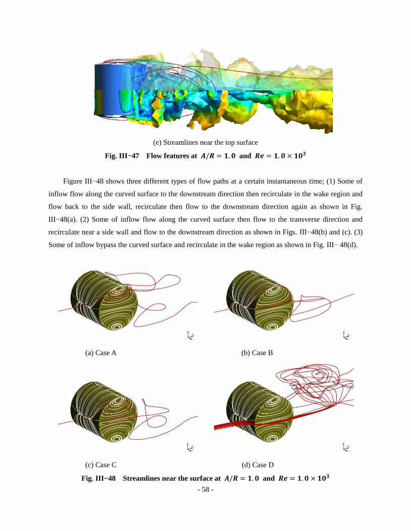
- 58 -

(e) Streamlines near the top surface

Fig. III−47 Flow features at and

Figure III−48 shows three different types of flow paths at a certain instantaneous time; (1) Some of

inflow flow along the curved surface to the downstream direction then recirculate in the wake region and

flow back to the side wall, recirculate then flow to the downstream direction again as shown in Fig.

III−48(a). (2) Some of inflow flow along the curved surface then flow to the transverse direction and

recirculate near a side wall and flow to the downstream direction as shown in Figs. III−48(b) and (c). (3)

Some of inflow bypass the curved surface and recirculate in the wake region as shown in Fig. III− 48(d).

(a) Case A (b) Case B

(c) Case C (d) Case D

Fig. III−48 Streamlines near the surface at and

- 59 -

Figure III−49 plots the velocity distributions on the x-y plane at different distances from the side

wall at the Reynolds number of and aspect ratio of 1.0. There is no more recirculating zone at

.

(a) Velocity distributions at (b) Velocity distributions at

(c) Velocity distributions at (d) Velocity distributions at

Fig. III−49 Velocity distributions at different locations ( and )

2. Parametric study

Figure III−50 shows the Strouhal number variations according to the variations of Reynolds numbers

at different aspect ratios. The Strouhal number of the drag force coefficient is higher than that of the lift

force coefficient or side force coefficient for all the aspect ratios and Reynolds numbers. In additions, the

Strouhal number of the lift force coefficient is higher than that of the side force coefficient. The Strouhal

number of the side force coefficient decreases as the aspect ratio increases at all the Reynolds numbers

because the side flow effect becomes weaker.

- 60 -

Fig. III−50 Strouhal number versus Reynolds number at different aspect ratios

The high mode Strouhal number for the drag force coefficient is observed at the Reynolds number of

for all the aspect ratios as shown in Fig. III−51. However, it is not observed at the lower

Reynolds number ranges including .

The high mode Strouhal number for the lift and side force coefficient is not observed at all the

Reynolds numbers and all the aspect ratios.

In general, the amplitude of the lift force coefficient of low frequency mode is much greater than that

of the drag force coefficient of low frequency mode as shown in Figure III−52. In addition, the amplitude

of the drag force coefficient of low frequency mode is greater than that of the drag force coefficient of

high frequency mode as shown in Figure III−51. If there exists a high frequency mode of the lift force

coefficient, the amplitude of the lift force coefficient of high frequency mode, which is directly related

with the amplitude of the drag force coefficient of high frequency mode , is much smaller than that of the

lift force coefficient of low frequency mode so that the high mode Strouhal number of the lift force

coefficient cannot be observed in FFT.

Unlike the streamwise directional flow or the upward / downward directional flow, the transverse

directional flow does not include any vortex sheet, which is detached from the curved body surface and

causes the high mode Strouhal number, so that no high mode Strouhal number of the side force coefficient

is observed in FFT.

From now on, we call the “low mode Strouhal number” for the drag force coefficient as simply

“Strouhal number”.

103

2x103

4x103

6x103

8x103

104

0.06

0.08

0.10

0.12

0.14

0.16

0.18

0.20

0.22

0.24

Str

ou

ha

l N

um

be

r

Reynolds Number

Drag(AR=1.0) Drag(AR=1.5) Drag(AR=2.0)

Lift(AR=1.0) Lift(AR=1.5) Lift(AR=2.0)

Side Force(AR=1.0) Side Force(AR=1.5) Side Force(AR=2.0)

- 61 -

(a) (b)

(c)

Fig. III−51 Fast Fourier Transform of oscillating drag force coefficient at

Figure III−52 plots the amplitude of force coefficient versus the Reynolds number at the different

aspect ratios. The amplitude of drag force coefficient has the minimum magnitude among the three

directional force coefficients no matter what the aspect ratios and Reynolds numbers are as might be

expected. The amplitude of the lift force coefficient is larger than that of the side force coefficient at the

same Reynolds number when the aspect ratios are 1.5 and 2.0, whereas the amplitude of the side force

coefficient is larger than that of the lift force coefficient at the aspect ratio of 1.0 because the vortex

shedding at the top and bottom surface occurs almost symmetrically with respect to the horizontal plane,

which means the amplitude of lift force coefficient becomes weaker. As the aspect ratio increases, the

amplitude of side force coefficient decreases at the Reynolds numbers of

because the side flow effect becomes weaker.

0.0 0.5 1.0 1.5 2.00.000

0.001

0.002

0.003

0.004

0.005

0.870Am

plit

ude

Strouhal Number

0.183

0.0 0.5 1.0 1.5 2.00.000

0.001

0.002

0.003

0.004

0.005

0.006

0.8240.664

Am

plit

ude

Strouhal Number

0.160

0.0 0.5 1.0 1.5 2.00.000

0.001

0.002

0.003

0.004

0.005

0.006

0.710

Am

plit

ude

Strouhal Number

0.137

- 62 -

Fig. III−52 Amplitude versus Reynolds number at different aspect ratios

Fig. III−53 Time averaged force coefficient versus Reynolds number at different aspect ratios

Figure III−53 compares the time averaged force coefficient. Time averaged drag force coefficient is

about 0.61 to 0.70 and increases as the aspect ratio increases at the same Reynolds number. On the other

hand, time averaged lift and side force coefficients are almost zero values at all the Reynolds numbers and

103

2x103

4x103

6x103

8x103

104

0.0

5.0x10-3

1.0x10-2

1.5x10-2

2.0x10-2

2.5x10-2

3.0x10-2

3.5x10-2

4.0x10-2

Am

plit

ud

e

Reynolds Number

Drag(AR=1.0) Drag(AR=1.5) Drag(AR=2.0)

Lift(AR=1.0) Lift(AR=1.5) Lift(AR=2.0)

Side Force(AR=1.0) Side Force(AR=1.5) Side Force(AR=2.0)

103

2x103

4x103

6x103

8x103

104

-0.2

0.0

0.2

0.4

0.6

0.8

Me

an

Fo

rce

Co

effic

ien

t

Reynolds Number

Drag(AR=1.0) Drag(AR=1.5) Drag(AR=2.0)

Lift(AR=1.0) Lift(AR=1.5) Lift(AR=2.0)

Side Force(AR=1.0) Side Force(AR=1.5) Side Force(AR=2.0)

- 63 -

all the aspect ratios.

Fig. III−54 Velocity profiles of time averaged streamwise velocity component at

Figure III−54 plots the velocity profiles of time averaged streamwise velocity component along the

z-direction at different distances from the body at the Reynolds number of . The recirculation

area on the plane becomes larger as the aspect ratio increases.

Fig. III−55 Velocity profiles of time averaged streamwise velocity component at

Figure III−55 plots the velocity profiles of time averaged streamwise velocity component along the

z-direction at different distances from the body at the aspect ratio of 2.0. The velocity profiles hardly

depend on the Reynolds numbers.

Figure III−56 plots the velocity profiles of time averaged streamwise velocity component along the

y-direction at different distances from the body at the Reynolds number of . The recirculation

region on the plane disappears faster as the aspect ratio decreases.

0.0 0.5 1.0

0

1

2

3

Vu /

z/D

A/R=1.0

A/R=1.5

A/R=2.0

x=0.6D

0.0 0.5 1.0

0

1

2

3

Vu /

z/D

x=0.8D

0.0 0.5 1.0

0

1

2

3

Vu /

z/D

x=1.6D

0.0 0.5 1.0

0

1

2

3

Vu /

z/D

x=3.2D

0.0 0.5 1.0

0

1

2

3

Vu /

z/D

x=6.4D

0.0 0.5 1.0

0

1

2

3

Vu /

z/D

Re=1,000

Re=2,000

Re=4,000

Re=10,000

x=0.6D

0.0 0.5 1.0

0

1

2

3

Vu /

z/D

x=0.8D

0.0 0.5 1.0

0

1

2

3

Vu /

z/D

x=1.6D

0.0 0.5 1.0

0

1

2

3

Vu /

z/D

x=3.2D

0.0 0.5 1.0

0

1

2

3

Vu /

z/D

x=6.4D

- 64 -

Fig. III−56 Velocity profiles of time averaged streamwise velocity component at

Figure III−57 plots the velocity profiles of time averaged streamwise velocity component along the

y-direction at different distances from the body at the aspect ratio of 2.0. The velocity profiles almost does

not depend on the Reynolds numbers.

Fig. III−57 Velocity profiles of time averaged streamwise velocity component at

3. Summary

The formation mechanism of the hairpin-shaped vortex shedding and the unsteady oscillating flow

phenomena are numerically investigated.

In general, the location of the vortex shedding is changed from time to time and rotates slowly and

irregularly about an axis through the center of the body. However, no rotating manner is observed for the

unsteady flow past a circular cylinder.

Unlike the vortex shedding behind a sphere or a rectangular parallelepiped, two different vortex

0.0 0.5 1.0

0

1

2

3

Vu /

y/D

A/R=1.0

A/R=1.5

A/R=2.0

x=0.6D

0.0 0.5 1.0

0

1

2

3

Vu /

y/D

x=0.8D

0.0 0.5 1.0

0

1

2

3

Vu /

y/D

x=1.6D

0.0 0.5 1.0

0

1

2

3

Vu /

y/D

x=3.2D

0.0 0.5 1.0

0

1

2

3

Vu /

y/D

x=6.4D

0.0 0.5 1.0

0

1

2

3

Vu /

y/D

Re=1,000

Re=2,000

Re=4,000

Re=10,000

x=0.6D

0.0 0.5 1.0

0

1

2

3

Vu /

y/D

x=0.8D

0.0 0.5 1.0

0

1

2

3

Vu /

y/D

x=1.6D

0.0 0.5 1.0

0

1

2

3

Vu /

y/D

x=3.2D

0.0 0.5 1.0

0

1

2

3

Vu /

y/D

x=6.4D

- 65 -

shedding patterns are observed depending on the aspect ratio of geometry; one is the symmetric-pair

vortex shedding pattern at the aspect ratio of 1.0 and the other is the alternating vortex shedding pattern at

the aspect ratio of 1.5 and 2.0 no matter what the Reynolds number is.

The drag force coefficient has high mode Strouhal number as well as low mode Strouhal number.

The high mode Strouhal number is observed only when the Reynolds number is for all the

aspect ratios. The (low mode) Strouhal number of the drag force coefficient is higher than that of lift force

coefficient or side force coefficient for all the aspect ratios and Reynolds numbers. The amplitude of the

drag force coefficient has the minimum magnitude among the three directional force coefficients no

matter what the aspect ratio and Reynolds number are. Time averaged drag force coefficient is about 0.61

to 0.70 and increases as the aspect ratio increases at the same Reynolds number.

The lift force coefficient has only low mode Strouhal number. The Strouhal number of the lift force

coefficient is higher than that of side force coefficient. The amplitude of lift force coefficient is larger than

that of the side force coefficient at the same Reynolds numbers when the aspect ratios are 1.5 and 2.0,

whereas the amplitude of lift force coefficient is smaller than that of the side force coefficient at the

aspect ratio of 1.0. Time averaged lift force coefficient is almost zero value at all the Reynolds numbers

and all the aspect ratios.

The side force coefficient has only low mode Strouhal number. The Strouhal number of the side

force coefficient is the lowest no matter what the aspect ratios and the Reynolds numbers are. The

Strouhal number of the side force coefficient decreases as the aspect ratio increases at all the Reynolds

numbers. The amplitude of the side force coefficient is smaller than that of the lift force coefficient except

at the aspect ratio of 1.0 for all the Reynolds numbers. As the aspect ratio increases, the amplitude of side

force coefficient decreases at the Reynolds numbers of . Time

averaged side force coefficient is almost zero value at all the Reynolds numbers and all the aspect ratios.

The size of recirculation region becomes larger as the aspect ratio increases. In addition, it disappears

faster along the downstream direction as the aspect ratio decreases. The Reynolds number does not affect

the size of recirculation region.

Finally, we can conclude that there are two different vortex shedding patterns depending on the

aspect ratio of the geometry and there is no rotating manner in the vortex shedding. The aspect ratio of

geometry affects the amplitude and Strouhal number of the side force coefficient, and the size of wake

region. The Reynolds number affects the existence of the high mode Strouhal number of the drag force

coefficient.

III-4. Overall Analysis

In this section, the Strouhal number and the amplitude of the oscillating forces, and time averaged

- 66 -

drag force coefficient are compared for the three different geometries such as sphere, rectangular

parallelepiped, and circular cylinder.

The shape of a sphere is approximately similar to the shape of a circular cylinder whose aspect ratio

is 1.0 so that the tendency of the numerical results is similar to each other as shown in Fig. III−58.

A sphere has the highest Strouhal number for the drag force, lift force, and side force coefficients.

The Strouhal number of the lift force coefficient for a circular cylinder whose aspect ratio is 1.0 is as high

as the Strouhal number of the lift force coefficient for a sphere.

(a) Drag force coefficient

(b) Lift force coefficient

Sphere Rec1.0 Rec1.5 Rec2.0 Cir1.0 Cir1.5 Cir2.00.00

0.04

0.08

0.12

0.16

0.20

0.24

Str

ouhal N

um

ber

Geometries

Re=1,000

Re=2,000

Re=4,000

Re=10,000

Sphere Rec1.0 Rec1.5 Rec2.0 Cir1.0 Cir1.5 Cir2.00.00

0.04

0.08

0.12

0.16

0.20

Str

ouhal N

um

ber

Geometries

Re=1,000

Re=2,000

Re=4,000

Re=10,000

- 67 -

(c) Side force coefficient

Fig. III−58 Strouhal number versus geometry

A rectangular parallelepiped has the lowest Strouhal number for the lift force and side force

coefficients. Namely, a sphere is the geometric shape which oscillates most frequently and a rectangular

parallelepiped is the geometric shape which oscillates most infrequently.

(a) Drag force coefficient

Sphere Rec1.0 Rec1.5 Rec2.0 Cir1.0 Cir1.5 Cir2.00.00

0.04

0.08

0.12

0.16

0.20

Str

ou

hal N

um

be

r

Geometries

Re=1,000

Re=2,000

Re=4,000

Re=10,000

Sphere Rec1.0 Rec1.5 Rec2.0 Cir1.0 Cir1.5 Cir2.00.000

0.002

0.004

0.006

0.008

0.010

Am

plit

ude

Geometries

Re=1,000

Re=2,000

Re=4,000

Re=10,000

- 68 -

(b) Lift force coefficient

(c) Side force coefficient

Fig. III−59 Amplitude versus geometry

Figure III−59 compares the amplitude versus geometry. The amplitude of the drag force coefficient

is generally very small so that it may be useless to investigate which geometry has the largest amplitude

even though a rectangular parallelepiped has the largest amplitude.

A rectangular parallelepiped has the largest amplitude of the lift force coefficient. The amplitude of

the side force coefficient decreases as the aspect ratio increases. If we confine the case which has the

aspect ratio of 1.0, a rectangular parallelepiped has the largest amplitude of the side force coefficient. And,

Sphere Rec1.0 Rec1.5 Rec2.0 Cir1.0 Cir1.5 Cir2.00.00

0.01

0.02

0.03

0.04

Am

plit

ude

Geometries

Re=1,000

Re=2,000

Re=4,000

Re=10,000

Sphere Rec1.0 Rec1.5 Rec2.0 Cir1.0 Cir1.5 Cir2.00.00

0.01

0.02

0.03

0.04

Am

plit

ude

Geometries

Re=1,000

Re=2,000

Re=4,000

Re=10,000

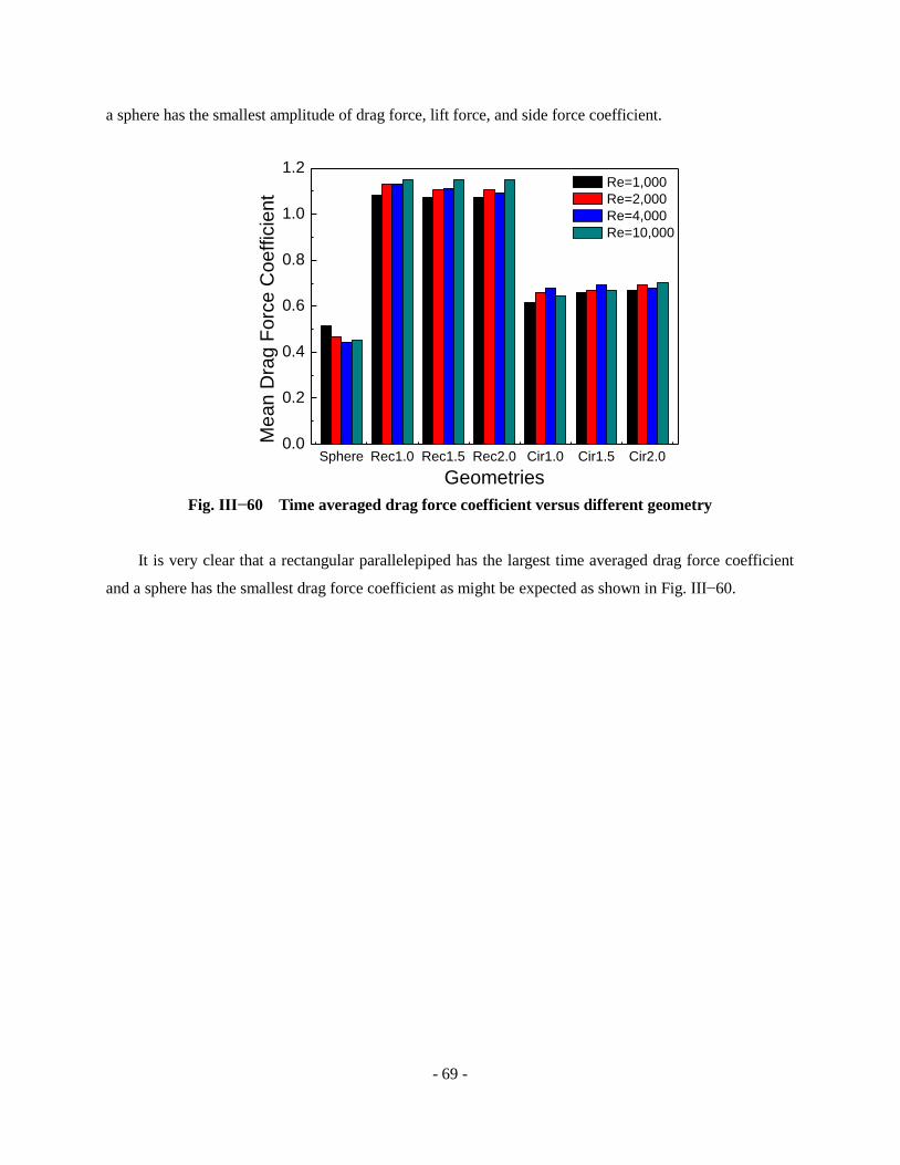
- 69 -

a sphere has the smallest amplitude of drag force, lift force, and side force coefficient.

Fig. III−60 Time averaged drag force coefficient versus different geometry

It is very clear that a rectangular parallelepiped has the largest time averaged drag force coefficient

and a sphere has the smallest drag force coefficient as might be expected as shown in Fig. III−60.

Sphere Rec1.0 Rec1.5 Rec2.0 Cir1.0 Cir1.5 Cir2.00.0

0.2

0.4

0.6

0.8

1.0

1.2

Mean D

rag F

orc

e C

oeffic

ient

Geometries

Re=1,000

Re=2,000

Re=4,000

Re=10,000

- 70 -

IV. CONCLUSIONS

The unsteady flowfield past a simplified MAV shaped geometry such as sphere, rectangular

parallelepiped, and circular cylinder has been analyzed numerically using Fluent to prepare a design

guideline for MAV. The mechanism of vortex shedding, the Strouhal number and the amplitude of the

oscillating drag, lift, and side force coefficient are studied in the range of Reynolds numbers from

to with three different aspect ratios of 1.0, 1.5, and 2.0.

Even though the mechanism of vortex shedding formation is very similar to each other, the vortex

shedding pattern has some differences. There exists a high mode Strouhal number of the drag force

coefficient for the flow past a sphere. However. there is no high mode Strouhal number for the flow past a

rectangular parallelepiped. In case of flow past a circular cylinder, there is a high mode Strouhal number

for the drag force coefficient only at the Reynolds number of . Actually, the amplitude of high

frequency mode is very tiny compared with other force coefficient amplitudes even though it has very

highly oscillating frequency.

In general, the vortex sheds form the body in randomly rotating pattern about an axis parallel to the

downstream direction through the center of the body. However, no rotating manner is observed for the

flow past a circular cylinder.

The vortex sheds alternately from the top and bottom surface for the flow past a sphere and a

rectangular parallelepiped. It also sheds alternately from the top and bottom surface for the flow past a

circular cylinder when the aspect ratios are 1.5 and 2.0. However, a symmetric-pair vortex shedding

occurs at the flow past a circular cylinder when the aspect ratio is 1.0 in the range of Reynolds numbers

from to .

Generally, the drag force coefficient has the highest Strouhal number meanwhile it has the least

amplitude. The amplitude of the lift force coefficient is the largest except for the flow past a circular

cylinder at the aspect ratio of 1.0. The amplitude of the side force coefficient decrease as the aspect ratio

increases for the flows past a rectangular parallelepiped and a circular cylinder. The Strouhal number of

the side force coefficient is the lowest in general.

A sphere has the highest Strouhal number for the drag force, lift force, and side force coefficients

where as a rectangular parallelepiped has the lowest Strouhal number for the drag force, lift force, and

side force coefficients. A rectangular parallelepiped has the largest amplitudes of the drag force, lift force,

and side force coefficient whereas a sphere has the smallest amplitudes of the drag force, lift force, and

side force coefficient. A rectangular parallelepiped also has the largest drag force coefficient.

As an additional remark, a very careful investigation is recommended for the flowfield analysis past

a geometry such as a rectangular parallelepiped or a circular cylinder whose aspect ratio is 1.0 because it

has strong three-dimensional geometric characters.

- 71 -

REFERENCES

[1] T. von Kármán, Uber den Mechanismus des Widerstandes den ein bewegter Korper in einer

Flussigkeit Erfahrt, Nachr. Ges. Wiss. Gottingen, Math-Phys Klasse, 12 (1912) 509-517.

[2] S. K. Jordan and J. E. Fromm, Oscillatory Drag, Lift, and Torque on a Circular Cylinder in a Uniform

Flow, Physics of Fluids, 15 (3) (1972) 371-376.

[3] H. M. Blackburn and R. D. Henderson, A study of two-dimensional flow past an oscillating cylinder,

Journal of Fluid Mechanics, 385 (1999) 255-286.

[4] R. Mittal and S. Balachandar, Direct Numerical Simulation of Flow Past Elliptic Cylinders, Journal of

Computational Physics, 124 (1996) 351-367.

[5] T. Ota, H. Nishiyama, and Y. Taoka, Flow Around an Elliptic Cylinder in the Critical Reynolds

Number Regime, Journal of Fluids Engineering, 109 (1987) 149-155.

[6] M. T. Nair and T. K. Sengupta, Onset of Asymmetry: Flow Past Circular and Elliptic Cylinders,

International Journal for Numerical Methods in Fluids, 23 (1996) 1327-1345.

[7] M. S. Kim and A. Sengupta, Unsteady Viscous Flow over Elliptic Cylinders at Various Thickness with

Different Reynolds Numbers, Journal of Mechanical Science and Technology, 19 (3) (2005) 877-886.

[8] V. A. Patel, Flow Around the Impulsively Started Elliptic Cylinder at Various Angles of Attack,

Computers and Fluids, 9 (4) (1981) 435-462.

[9] M. H. Chou and W. Huang, Numerical Study of High-Reynolds-Number Flow Past a Blunt Object,

International Journal for Numerical Methods in Fluids, 23 (1996) 711-732.

[10] H. M. Badr, S. C. R. Dennis, and S. Kocabiyik, Numerical simulation of the unsteady flow over an

elliptic cylinder at different orientations, International Journal for Numerical Methods in Fluids, 37

(2001) 905-931.

[11] M. S. Kim and Y. B. Park, Unsteady Lift and Drag Forces Acting on the Elliptic Cylinder, Journal of

Mechanical Science and Technology, 20 (1) (2006) 167-175.

[12] R. W. Davis and E. F. Moore, A numerical study of vortex shedding from rectangles, Journal of

Mechanics, 116 (1982) 475-506.

[13] A. Okajima, Strouhal numbers of rectangular cylinders, Journal of Fluid Mechanics, 123 (1982) 379-

398.

[14] C. Norberg, Flow around rectangular cylinders: Pressure forces and wake frequencies, Journal of

Wind Engineering and Industrial Aerodynamics, 49 (1993) 187-196.

[15] A. Sohankar, C. Norberg, and L. Davidson, LOW-REYNOLDS-NUMBER FLOW AROUND A

SQUARE CYLINDER AT INCIDENCE: STUDY OF BLOCKAGE, ONSET OF VORTEX SHEDDING

AND OUTLET BOUNDARY CONDITION, International Journal for numerical methods in fluids, 26

(1998) 39-56.

- 72 -

[16] R. Mittal & F. M. Najjar, Vortex Dynamics in the Sphere Wake, AIAA-99-3806.

[17] D. A. Jones and D. B. Clarke, Simulation of Flow Past a Sphere using the Fluent Code, DSTO-TR-

2232 (2008) 1-35.

[18] T. A. Johnson and V. C. Patel, Flow past a sphere up to a Reynolds number of 300, Journal of Fluid

Mechanics , 378 (1999) 19-70.

[19] A. G. Tomboulides, S. A. Orszag, and G. E. Karniadakis, Direct and Large-Eddy Simulation of

Axisymmetric Wakes, AIAA-93-0546.

[20] A. G. Tomboulides and S. A. Orszag, Numerical investigation of transitional and weak turbulent flow

past a sphere, Journal of Fluid Mechanics, 416 (2000) 45-73.

[21] G. Constantinescu and K. Squires, Numerical investigations of flow over a sphere in the subcritical

and supercritical regimes, Physics of Fluids, 16 (5) (2004) 1449-1466.

[22] S. Taneda, Visual observations of the flow past a sphere at Reynolds numbers between

and , Journal of Fluid Mechanics, 85 (1978) 187-192.

[23] H. Sakamoto and H. Haniu, A Study on Vortex Shedding From Spheres in a Uniform Flow, Journal

of Fluids Engineering, 112 (1990) 386-392.

[24] G. Constantinescu, M. Chapelet, and K. Squires, Turbulence Modeling Applied to Flow over a

Sphere, AIAA Journal, 41 (9) (2003) 1733-1742.

[25] G. Constantinescu and K. Squires, LES and DES Investigations of Turbulent Flow over a Sphere at

Re=10,000, Flow, Turbulence and Combustion, 70 (2003) 267-298.

[26] H. Sakamoto and H. Haniu, The formation mechanism and shedding frequency of vortices from a

sphere in uniform shear flow, Journal of Fluid Mechanics, 287 (1995) 151-171.

[27] E. Achenbach, Vortex shedding from spheres, Journal of Fluid Mechanics, 62 (1974) 209-221.

[28] S. Taneda, Experimental Investigation of the Wake behind a Sphere at Low Reynolds Numbers,

Journal of the Physical Society of Japan, 11 (10) (1956) 1104-1108.

[29] V. Bakic, M. Schmid, and B. Stankovic, EXPERIMENTAL INVESTIGATION OF TURBULENT

STRUCTURES OF FLOW AROUND A SPHERE, Thermal Science, 10 (2) (2006) 97-112.

[30] S. Krajnovic and L. Davison, Large-Eddy Simulation of the Flow Around a Bluff Body, AIAA

Journal, 40 (5) (2002) 927-936.

[31] S. Krajnovic and L. Davison, DEVELOPMENT OF LARGE-EDDY SIMULATION FOR VEHICLE

AERODYNAMICS, ASME International Mechanical Engineering Congress & Exposition, IMECE2002-

32833.

[32] G. Iaccarino and P. Durbin, Unsteady 3D RANS simulations using the model, Center for

Turbulence Research, Anual Research Briefs 2000 263-269.

[33] S. Vengadesan and A. Nakayama, Evaluation of LES models for flow over bluff body from

- 73 -

engineering application perspective, Sadhana, 30 (2005) 11-20.

[34] S. Murakami and A. Mochida, On turbulent vortex shedding flow past 2D square cylinder predicted

by CFD, Journal of Wind Engineering and Industrial Aerodynamics, 54/55 (1995) 191-211.

[35] K Luo, J. Fan, W. Li, and K. Cen, Transient, three-dimensional simulation of particle dispersion in

flows around a circular cylinder ( ), Fuel, 88 (2009) 1294-1301.

[36] V. Karlo and T. Tezduyar, Parallel 3D computation of unsteady flows around circular cylinders,

Parallel Computing, 23 (1997) 1235-1248.

[37] M. Zhao, L. Cheng, and T. Zhou, Direct numerical simulation of three-dimensional flow past a

yawed circular cylinder of infinite length, Journal of Fluids and Structures, (2009)

doi:10.1016/j.jfluidstructs.2009.02.004.

[38] D. Yeo and N. P. Jones, Investigation on 3-D characteristics of flow around a yawed and inclined

circular cylinder, Journal of Wind Engineering and Industrial Aerodynamics, 96 (2008) 1947-1960.

[39] H. Persillon and M. Braza, Physical analysis of the transition to turbulence in the wake of a circular

cylinder by three-dimensional Navier-Stokes simulation, Journal of Fluid Mechanics, 365 (1998) 23-88.

[40] J. G. Wissink and W. Rodi, Numerical study of the near wake of a circular cylinder, International

Journal of Heat and Fluid Flow, 29 (2008) 1060-1070.

[41] J. M. McMichael and M. S. Francis, Micro Air Vehicle – Toward a New Dimension in Flight,

http://www.fas.org/irp/program/collect/docs/mav_auvsi.htm

[42] D. J. Patil, I. M. Khan, and B. K. Gupta, Numerical Simulations of Low Reynolds Number Flow

Around Micro Air Vehicle, Proceedings of the International Conference on Aerospace Science and

Technology, INCAST 2008-054.

[43] Fluent, http://www.fluent.com/

[44] CFX, http://www.ansys.com/products/fluid-dynamics/cfx/yy

[45] P. R. Spalart and S. R. Allmaras, A ONE-EQUATION TURBULENCE MODEL FOR

AERODYNAMIC FLOWS, Boring Commercial Airplane Group.

[46] W. P. Jones and B. E. Launder, THE PREDICTION OF LAMINARIZATION WITH A TWO-

EQUATION MODEL OF TURBULENCE, International Journal of Heat and Mass Transfer, 15 (1972)

301-314.

[47] G. Iaccarino, A. Ooi, P. A. Durbin, and M. Behnia, Reynolds averaged simulation of unsteady

separated flow, International Journal of Heat and Fluid Flow, 24 (2003) 147-156.

[48] J. Smagorinsky, GENERAL CIRCULATION EXPERIMENTS WITH THE PRIMITIVE

EQUATIONS, Monthly Weather Review, 91 (3) (1963) 99-164.

[49] P. R. Spalart, Strategies for turbulence modeling and simulations, International Journal of Heat and

Fluid Flow, 21 (2000) 252-263.

- 74 -

[50] F. R. Menter, Two-Equation Eddy-Viscosity Turbulence Models for Engineering Applications, AIAA

Journal, 32 (8) (1994) 1598-1605.

[51] J. C. R. Hunt, A. A. Wary, and P. Moin, Eddies, Streams, and Convergence Zones in Turbulent Flows,

Proceedings for the summer program 1988, (1988) 193-208.

- 75 -

APPENDIX A - Sphere

Fig. A1 Time history of unsteady drag force coefficient

(a) (b)

(c) (d)

Fig. A2 Power spectrum of drag force coefficient

0 10 20 30 400.35

0.40

0.45

0.50

0.55

0.60

0.65

Cd

Time(T*)

Re=1,000

Re=2,000

Re=4,000

Re=10,000

0.0 0.5 1.0 1.5 2.00.000

0.001

0.002

0.003

0.004

0.005

0.35

Am

plit

ude

Strouhal Number

0.18

0.0 0.5 1.0 1.5 2.00.000

0.001

0.002

0.003

0.004

0.005

0.50

0.19

Am

plit

ude

Strouhal Number

0.0 0.5 1.0 1.5 2.00.000

0.001

0.002

0.003

0.004

0.005

0.81

0.19

Am

plit

ude

Strouhal Number

0.0 0.5 1.0 1.5 2.00.000

0.001

0.002

0.003

0.004

0.0050.20

Am

plit

ude

Strouhal Number

- 76 -

Fig. A3 Time history of unsteady lift force coefficient

(a) (b)

(c) (d)

Fig. A4 Power spectrum of lift force coefficient

0 10 20 30 40-0.4

-0.3

-0.2

-0.1

0.0

0.1

0.2

0.3

0.4

Cl

Time(T*)

Re=1,000

Re=2,000

Re=4,000

Re=10,000

0.0 0.5 1.0 1.5 2.00.000

0.005

0.010

0.015

0.020

0.025

0.030

0.140

Am

plit

ude

Strouhal Number

0.0 0.5 1.0 1.5 2.00.000

0.005

0.010

0.015

0.020

0.025

0.030

0.114

Am

plit

ude

Strouhal Number

0.0 0.5 1.0 1.5 2.00.000

0.005

0.010

0.015

0.020

0.025

0.030

0.160

Am

plit

ude

Strouhal Number

0.0 0.5 1.0 1.5 2.00.000

0.005

0.010

0.015

0.020

0.025

0.030

Am

plit

ude

Strouhal Number

0.15

- 77 -

Fig. A5 Time history of unsteady side force coefficient

(a) (b)

(c) Re (d)

Fig. A6 Power spectrum of side force coefficient

0 10 20 30 40-0.4

-0.3

-0.2

-0.1

0.0

0.1

0.2

0.3

0.4

Cs

Time(T*)

Re=1,000

Re=2,000

Re=4,000

Re=10,000

0.0 0.5 1.0 1.5 2.00.000

0.005

0.010

0.015

0.020

0.025

0.030

0.157Am

plit

ude

Strouhal Number

0.0 0.5 1.0 1.5 2.00.000

0.005

0.010

0.015

0.020

0.025

0.030

0.157

Am

plit

ude

Strouhal Number

0.0 0.5 1.0 1.5 2.00.000

0.005

0.010

0.015

0.020

0.025

0.030

Am

plit

ude

Strouhal Number

0.144

0.0 0.5 1.0 1.5 2.00.000

0.005

0.010

0.015

0.020

0.025

0.030

0.175

Am

plit

ude

Strouhal Number

- 78 -

(a) (T*=20)

(b) (T*=20)

(c) (T*=15)

(d) (T*=20)

Fig. A7 Oil flows on the top and bottom surface with same legend of skin friction coefficient

- 79 -

(a)

(b)

(c)

(d)

Fig.A8 Vortex structure (side view and top view)

- 80 -

APPENDIX B – Rectangular Parallelepiped

(a) Drag force coefficient

(b) Lift force coefficient

(c) Side force coefficient

Fig. B1 Time history of unsteady force coefficient at

0 10 20 30 401.00

1.05

1.10

1.15

1.20

1.25

1.30

Cd

Time(T*)

A/R = 1.0

A/R = 1.5

A/R = 2.0

0 10 20 30 40

-0.1

0.0

0.1

0.2

0.3

Cl

Time(T*)

A/R = 1.0

A/R = 1.5

A/R = 2.0

0 10 20 30 40

-0.1

0.0

0.1

0.2

0.3

Cs

Time(T*)

A/R = 1.0

A/R = 1.5

A/R = 2.0

- 81 -

(a) Drag force coefficient (b)

(c) (d)

Fig. B2 Power spectrum of drag force coefficient at

0 10 20 30 401.00

1.05

1.10

1.15

1.20

1.25

1.30

Cd

Time(T*)

A/R = 1.0

A/R = 1.5

A/R = 2.0

0.0 0.5 1.0 1.5 2.00.000

0.001

0.002

0.003

0.004

0.005

0.006

0.007

Am

plit

ude

Strouhal Number

0.149

0.0 0.5 1.0 1.5 2.00.000

0.001

0.002

0.003

0.004

0.005

0.006

0.007

Am

plit

ude

Strouhal Number

0.128

0.0 0.5 1.0 1.5 2.00.000

0.001

0.002

0.003

0.004

0.005

0.006

0.007

Am

plit

ude

Strouhal Number

0.101

- 82 -

(a) Lift force coefficient (b)

(c) (d)

Fig. B3 Power spectrum of lift force coefficient at

0 10 20 30 40

-0.1

0.0

0.1

0.2

0.3

Cl

Time(T*)

A/R = 1.0

A/R = 1.5

A/R = 2.0

0.0 0.5 1.0 1.5 2.00.000

0.005

0.010

0.015

0.020

0.025

0.030

0.035

0.040

Am

plit

ude

Strouhal Number

0.117

0.0 0.5 1.0 1.5 2.00.000

0.005

0.010

0.015

0.020

0.025

0.030

0.035

0.040

Am

plit

ude

Strouhal Number

0.085

0.0 0.5 1.0 1.5 2.00.000

0.005

0.010

0.015

0.020

0.025

0.030

0.035

0.040

Am

plit

ude

Strouhal Number

0.089

- 83 -

(a) Side force coefficient (b)

(c) (d)

Fig. B4 Power spectrum of side force coefficient at

0 10 20 30 40

-0.1

0.0

0.1

0.2

0.3

Cs

Time(T*)

A/R = 1.0

A/R = 1.5

A/R = 2.0

0.0 0.5 1.0 1.5 2.00.000

0.005

0.010

0.015

0.020

0.025

0.030

0.035

0.040

Am

plit

ude

Strouhal Number

0.097

0.0 0.5 1.0 1.5 2.00.000

0.005

0.010

0.015

0.020

0.025

0.030

0.035

0.040

Am

plit

ude

Strouhal Number

0.064

0.0 0.5 1.0 1.5 2.00.000

0.005

0.010

0.015

0.020

0.025

0.030

0.035

0.040

Am

plit

ude

Strouhal Number

0.068

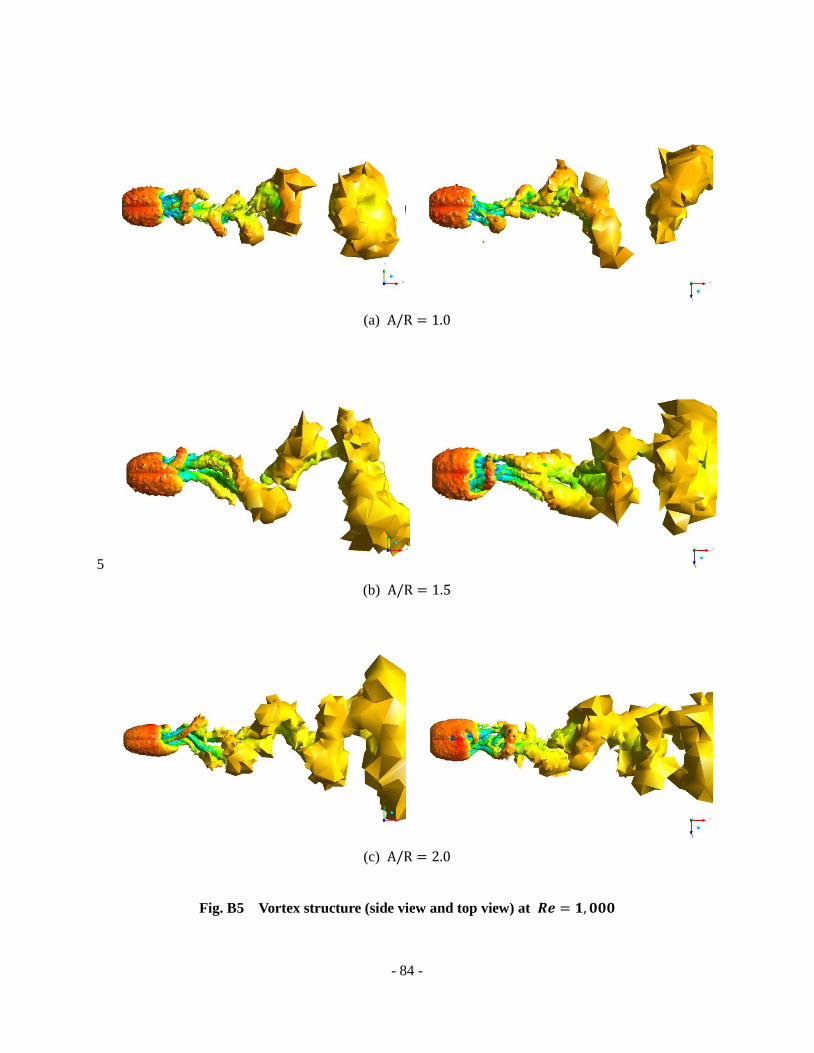
- 84 -

(a)

5

(b)

(c)

Fig. B5 Vortex structure (side view and top view) at

- 85 -

(a) Drag force coefficient

(b) Lift force coefficient

(c) Side force coefficient

Fig. B6 Time history of unsteady force coefficient at

0 10 20 30 401.00

1.05

1.10

1.15

1.20

1.25

1.30

Cd

Time(T*)

A/R = 1.0

A/R = 1.5

A/R = 2.0

0 10 20 30 40

-0.1

0.0

0.1

0.2

0.3

Cl

Time(T*)

A/R = 1.0

A/R = 1.5

A/R = 2.0

0 10 20 30 40

-0.1

0.0

0.1

0.2

0.3

Cs

Time(T*)

A/R = 1.0

A/R = 1.5

A/R = 2.0

- 86 -

(a) Drag force coefficient (b)

(c) (d)

Fig. B7 Power spectrum of drag force coefficient at

0 10 20 30 401.00

1.05

1.10

1.15

1.20

1.25

1.30

Cd

Time(T*)

A/R = 1.0

A/R = 1.5

A/R = 2.0

0.0 0.5 1.0 1.5 2.00.000

0.001

0.002

0.003

0.004

0.005

0.006

0.007

0.146

Am

plit

ude

Strouhal Number

0.0 0.5 1.0 1.5 2.00.000

0.001

0.002

0.003

0.004

0.005

0.006

0.007

0.126

Am

plit

ude

Strouhal Number

- 87 -

(a) Lift force coefficient (b)

(c) (d)

Fig. B8 Power spectrum of lift force coefficient at

0 10 20 30 40

-0.1

0.0

0.1

0.2

0.3

Cl

Time(T*)

A/R = 1.0

A/R = 1.5

A/R = 2.0

0.0 0.5 1.0 1.5 2.00.000

0.005

0.010

0.015

0.020

0.025

0.030

0.035

0.040

Am

plit

ude

Strouhal Number

0.117

0.0 0.5 1.0 1.5 2.00.000

0.005

0.010

0.015

0.020

0.025

0.030

0.035

0.040

Am

plit

ude

Strouhal Number

0.086

0.0 0.5 1.0 1.5 2.00.000

0.005

0.010

0.015

0.020

0.025

0.030

0.035

0.040

Am

plit

ude

Strouhal Number

0.101

- 88 -

(a) Side force coefficient (b)

(c) (d) .

Fig. B9 Power spectrum of side force coefficient at

0 10 20 30 40

-0.1

0.0

0.1

0.2

0.3

Cs

Time(T*)

A/R = 1.0

A/R = 1.5

A/R = 2.0

0.0 0.5 1.0 1.5 2.00.000

0.005

0.010

0.015

0.020

0.025

0.030

0.035

0.040

Am

plit

ude

Strouhal Number

0.087

0.0 0.5 1.0 1.5 2.00.000

0.005

0.010

0.015

0.020

0.025

0.030

0.035

0.040

Am

plit

ude

Strouhal Number

0.058

0.0 0.5 1.0 1.5 2.00.000

0.005

0.010

0.015

0.020

0.025

0.030

0.035

0.040

Am

plit

ude

Strouhal Number

0.076

- 89 -

(a)

(b)

(c)

Fig. B10 Vortex structure (side view and top view) at

- 90 -

(a) Drag force coefficient

(b) Lift force coefficient

(c) Side force coefficient

Fig. B11 Time history of unsteady force coefficient at

0 10 20 30 401.00

1.05

1.10

1.15

1.20

1.25

1.30

Cd

Time(T*)

A/R = 1.0

A/R = 1.5

A/R = 2.0

0 10 20 30 40

-0.1

0.0

0.1

0.2

0.3

Cl

Time(T*)

A/R = 1.0

A/R = 1.5

A/R = 2.0

0 10 20 30 40

-0.1

0.0

0.1

0.2

0.3

Cs

Time(T*)

A/R = 1.0

A/R = 1.5

A/R = 2.0

- 91 -

(a) Drag force coefficient (b)

(c) (d)

Fig. B12 Power spectrum of drag force coefficient at

0 10 20 30 401.00

1.05

1.10

1.15

1.20

1.25

1.30

Cd

Time(T*)

A/R = 1.0

A/R = 1.5

A/R = 2.0

0.0 0.5 1.0 1.5 2.00.000

0.001

0.002

0.003

0.004

0.005

0.006

0.0070.150

Am

plit

ude

Strouhal Number

0.0 0.5 1.0 1.5 2.00.000

0.001

0.002

0.003

0.004

0.005

0.006

0.0070.162

Am

plit

ude

Strouhal Number

0.0 0.5 1.0 1.5 2.00.000

0.001

0.002

0.003

0.004

0.005

0.006

0.007

0.146

Am

plit

ude

Strouhal Number

- 92 -

(a) Lift force coefficient (b)

(c) (d)

Fig. B13 Power spectrum of Lift force coefficient at

0 10 20 30 40

-0.1

0.0

0.1

0.2

0.3

Cl

Time(T*)

A/R = 1.0

A/R = 1.5

A/R = 2.0

0.0 0.5 1.0 1.5 2.00.000

0.005

0.010

0.015

0.020

0.025

0.030

0.035

0.040

Am

plit

ude

Strouhal Number

0.1

0.0 0.5 1.0 1.5 2.00.000

0.005

0.010

0.015

0.020

0.025

0.030

0.035

0.040

Am

plit

ude

Strouhal Number

0.081

0.0 0.5 1.0 1.5 2.00.000

0.005

0.010

0.015

0.020

0.025

0.030

0.035

0.040

Am

plit

ude

Strouhal Number

0.087

- 93 -

(a) Side force coefficient (b)

(c) (d)

Fig. B14 Power spectrum of Side force coefficient at

0 10 20 30 40

-0.1

0.0

0.1

0.2

0.3

Cs

Time(T*)

A/R = 1.0

A/R = 1.5

A/R = 2.0

0.0 0.5 1.0 1.5 2.00.000

0.005

0.010

0.015

0.020

0.025

0.030

0.035

0.040

Am

plit

ude

Strouhal Number

0.1

0.0 0.5 1.0 1.5 2.00.000

0.005

0.010

0.015

0.020

0.025

0.030

0.035

0.040

Am

plit

ude

Strouhal Number

0.069

0.0 0.5 1.0 1.5 2.00.000

0.005

0.010

0.015

0.020

0.025

0.030

0.035

0.040

Am

plit

ude

Strouhal Number

0.058

- 94 -

(a)

(b)

(c)

Fig. B15 Vortex structure (side view and top view) at

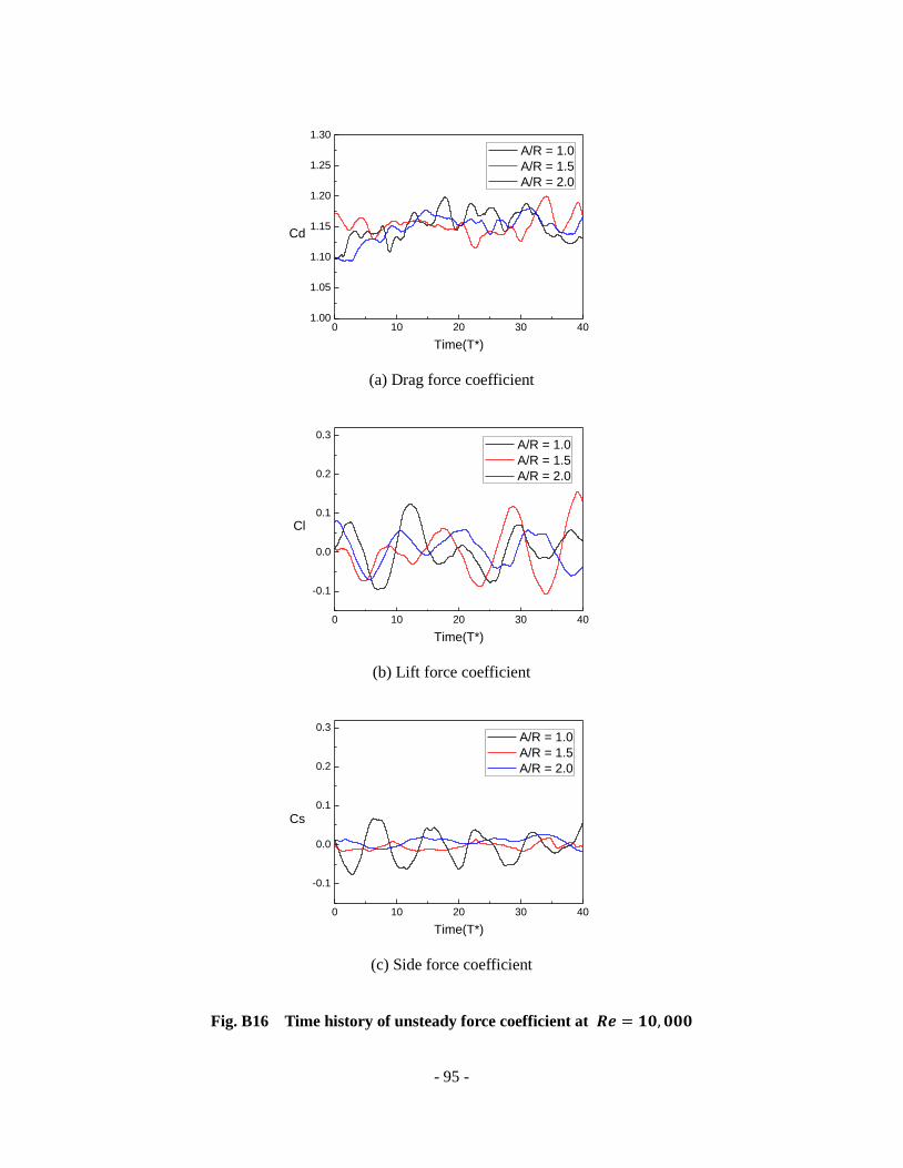
- 95 -

(a) Drag force coefficient

(b) Lift force coefficient

(c) Side force coefficient

Fig. B16 Time history of unsteady force coefficient at

0 10 20 30 401.00

1.05

1.10

1.15

1.20

1.25

1.30

Cd

Time(T*)

A/R = 1.0

A/R = 1.5

A/R = 2.0

0 10 20 30 40

-0.1

0.0

0.1

0.2

0.3

Cl

Time(T*)

A/R = 1.0

A/R = 1.5

A/R = 2.0

0 10 20 30 40

-0.1

0.0

0.1

0.2

0.3

Cs

Time(T*)

A/R = 1.0

A/R = 1.5

A/R = 2.0

- 96 -

(a) Drag force coefficient (b)

(c) (d)

Fig. B17 Power spectrum of drag force coefficient at

0 10 20 30 401.00

1.05

1.10

1.15

1.20

1.25

1.30

Cd

Time(T*)

A/R = 1.0

A/R = 1.5

A/R = 2.0

0.0 0.5 1.0 1.5 2.00.000

0.001

0.002

0.003

0.004

0.005

0.006

0.007

0.149

Am

plit

ude

Strouhal Number

0.0 0.5 1.0 1.5 2.00.000

0.001

0.002

0.003

0.004

0.005

0.006

0.007

0.137

Am

plit

ude

Strouhal Number

0.0 0.5 1.0 1.5 2.00.000

0.001

0.002

0.003

0.004

0.005

0.006

0.007

0.125A

mplit

ude

Strouhal Number

- 97 -

(a) Side force coefficient (b)

(c) (d)

Fig. B18 Power spectrum of lift force coefficient at

0 10 20 30 40

-0.1

0.0

0.1

0.2

0.3

Cl

Time(T*)

A/R = 1.0

A/R = 1.5

A/R = 2.0

0.0 0.5 1.0 1.5 2.00.000

0.005

0.010

0.015

0.020

0.025

0.030

0.035

0.040

Am

plit

ude

Strouhal Number

0.1

0.0 0.5 1.0 1.5 2.00.000

0.005

0.010

0.015

0.020

0.025

0.030

0.035

0.040

Am

plit

ude

Strouhal Number

0.11

0.0 0.5 1.0 1.5 2.00.000

0.005

0.010

0.015

0.020

0.025

0.030

0.035

0.040

Am

plit

ude

Strouhal Number

0.1

- 98 -

(a) Side force coefficient (b)

(c) (d)

Fig. B19 Power spectrum of side force coefficient at

0 10 20 30 40

-0.1

0.0

0.1

0.2

0.3

Cs

Time(T*)

A/R = 1.0

A/R = 1.5

A/R = 2.0

0.0 0.5 1.0 1.5 2.00.000

0.005

0.010

0.015

0.020

0.025

0.030

0.035

0.040

Am

plit

ude

Strouhal Number

0.125

0.0 0.5 1.0 1.5 2.00.000

0.005

0.010

0.015

0.020

0.025

0.030

0.035

0.040

Am

plit

ude

Strouhal Number

0.082

0.0 0.5 1.0 1.5 2.00.000

0.005

0.010

0.015

0.020

0.025

0.030

0.035

0.040

Am

plit

ude

Strouhal Number

0.10

- 99 -

(a)

(b)

(c)

Fig. B20 Vortex structure (side view and top view) at

- 100 -

APPENDIX C – Circular Cylinder

(a) Drag force coefficient

(b) Lift force coefficient

(c) Side force coefficient

Fig. C1 Time history of unsteady force coefficient at

0 10 20 30 40 500.55

0.60

0.65

0.70

0.75

Cd

Time(T*)

A/R = 1.0

A/R = 1.5

A/R = 2.0

0 10 20 30 40 50-0.15

-0.10

-0.05

0.00

0.05

0.10

0.15

Cl

Time(T*)

A/R = 1.0

A/R = 1.5

A/R = 2.0

0 10 20 30 40 50-0.15

-0.10

-0.05

0.00

0.05

0.10

0.15

Cs

Time(T*)

A/R = 1.0

A/R = 1.5

A/R = 2.0

- 101 -

(a) Drag force coefficient (b)

(c) (d)

Fig. C2 Power spectrum of drag force coefficient at

0 10 20 30 40 500.55

0.60

0.65

0.70

0.75

Cd

Time(T*)

A/R = 1.0

A/R = 1.5

A/R = 2.0

0.0 0.5 1.0 1.5 2.00.000

0.001

0.002

0.003

0.004

0.005

0.006

Am

plit

ude

Strouhal Number

0.139

0.0 0.5 1.0 1.5 2.00.000

0.001

0.002

0.003

0.004

0.005

Am

plit

ude

Strouhal Number

0.160

0.0 0.5 1.0 1.5 2.00.000

0.001

0.002

0.003

0.004

0.005

Am

plit

ude

Strouhal Number

0.137

- 102 -

(a) Lift force coefficient (b)

(c) (d)

Fig. C3 Power spectrum of lift force coefficient at

0 10 20 30 40 50-0.15

-0.10

-0.05

0.00

0.05

0.10

0.15

Cl

Time(T*)

A/R = 1.0

A/R = 1.5

A/R = 2.0

0.0 0.5 1.0 1.5 2.00.000

0.005

0.010

0.015

0.020

0.025

0.030

Am

plit

ude

Strouhal Number

0.110

0.0 0.5 1.0 1.5 2.00.000

0.005

0.010

0.015

0.020

0.025

0.030

Am

plit

ude

Strouhal Number

0.119

0.0 0.5 1.0 1.5 2.00.000

0.005

0.010

0.015

0.020

0.025

0.030

Am

plit

ude

Strouhal Number

0.080

- 103 -

(a) Side force coefficient (b)

(c) (d)

Fig. C4 Power spectrum of side force coefficient at

0 10 20 30 40 50-0.15

-0.10

-0.05

0.00

0.05

0.10

0.15

Cs

Time(T*)

A/R = 1.0

A/R = 1.5

A/R = 2.0

0.0 0.5 1.0 1.5 2.00.000

0.005

0.010

0.015

0.020

0.025

0.030

Am

plit

ude

Strouhal Number

0.110

0.0 0.5 1.0 1.5 2.00.000

0.005

0.010

0.015

0.020

0.025

0.030

Am

plit

ude

Strouhal Number

0.092

0.0 0.5 1.0 1.5 2.00.000

0.005

0.010

0.015

0.020

0.025

0.030

Am

plit

ude

Strouhal Number

0.079

- 104 -

(a)

(b)

(c)

Fig. C5 Vortex structure (side view and top view) at

- 105 -

(a) Drag force coefficient

(b) Lift force coefficient

(c) Side force coefficient

Fig. C6 Time history of unsteady force coefficient at

0 10 20 30 40 500.60

0.65

0.70

0.75

Cd

Time(T*)

A/R = 1.0

A/R = 1.5

A/R = 2.0

0 10 20 30 40 50-0.15

-0.10

-0.05

0.00

0.05

0.10

0.15

Cl

Time(T*)

A/R = 1.0

A/R = 1.5

A/R = 2.0

0 10 20 30 40 50-0.15

-0.10

-0.05

0.00

0.05

0.10

0.15

0.20

0.25

Cs

Time(T*)

A/R = 1.0

A/R = 1.5

A/R = 2.0

- 106 -

(a) Drag force coefficient (b)

(c) (d)

Fig. C7 Power spectrum of drag force coefficient at

0 10 20 30 40 500.60

0.65

0.70

0.75

Cd

Time(T*)

A/R = 1.0

A/R = 1.5

A/R = 2.0

0.0 0.5 1.0 1.5 2.00.000

0.001

0.002

0.003

0.004

0.005

Am

plit

ude

Strouhal Number

0.139

0.0 0.5 1.0 1.5 2.00.000

0.001

0.002

0.003

0.004

0.005

0.006

Am

plit

ude

Strouhal Number

0.125

0.0 0.5 1.0 1.5 2.00.000

0.001

0.002

0.003

0.004

0.005

Am

plit

ude

Strouhal Number

0.117

- 107 -

(a) Lift force coefficient (b)

(c) (d)

Fig. C8 Power spectrum of lift force coefficient at

0 10 20 30 40 50-0.15

-0.10

-0.05

0.00

0.05

0.10

0.15

Cl

Time(T*)

A/R = 1.0

A/R = 1.5

A/R = 2.0

0.0 0.5 1.0 1.5 2.00.000

0.005

0.010

0.015

0.020

0.025

0.030

Am

plit

ude

Strouhal Number

0.128

0.0 0.5 1.0 1.5 2.00.000

0.005

0.010

0.015

0.020

0.025

0.030

Am

plit

ude

Strouhal Number

0.137

0.0 0.5 1.0 1.5 2.00.000

0.005

0.010

0.015

0.020

0.025

0.030

Am

plit

ude

Strouhal Number

0.122

- 108 -

(a) Side force coefficient (b)

(c) (d)

Fig. C9 Power spectrum of side force coefficient at

0 10 20 30 40 50-0.15

-0.10

-0.05

0.00

0.05

0.10

0.15

0.20

0.25

Cs

Time(T*)

A/R = 1.0

A/R = 1.5

A/R = 2.0

0.0 0.5 1.0 1.5 2.00.000

0.005

0.010

0.015

0.020

0.025

0.030

Am

plit

ude

Strouhal Number

0.105

0.0 0.5 1.0 1.5 2.00.000

0.005

0.010

0.015

0.020

0.025

0.030

Am

plit

ude

Strouhal Number

0.075

0.0 0.5 1.0 1.5 2.00.000

0.005

0.010

0.015

0.020

0.025

0.030

Am

plit

ude

Strouhal Number

0.078

- 109 -

(a)

(b)

(c)

Fig. C10 Vortex structure (side view and top view) at

- 110 -

(a) Drag force coefficient

(b) Lift force coefficient

(c) Side force coefficient

Fig. C11 Time history of unsteady force coefficient at

0 10 20 30 40 500.60

0.65

0.70

0.75

0.80

Cd

Time(T*)

A/R = 1.0

A/R = 1.5

A/R = 2.0

0 10 20 30 40 50-0.20

-0.15

-0.10

-0.05

0.00

0.05

0.10

0.15

0.20

Cl

Time(T*)

A/R = 1.0

A/R = 1.5

A/R = 2.0

0 10 20 30 40 50-0.20

-0.15

-0.10

-0.05

0.00

0.05

0.10

0.15

0.20

Cs

Time(T*)

A/R = 1.0

A/R = 1.5

A/R = 2.0

- 111 -

(a) Drag force coefficient (b)

(c) (d)

Fig. C12 Power spectrum of drag force coefficient at

0 10 20 30 40 500.60

0.65

0.70

0.75

0.80

Cd

Time(T*)

A/R = 1.0

A/R = 1.5

A/R = 2.0

0.0 0.5 1.0 1.5 2.00.000

0.001

0.002

0.003

0.004

0.005

Am

plit

ude

Strouhal Number

0.20

0.0 0.5 1.0 1.5 2.00.000

0.001

0.002

0.003

0.004

0.005

0.006

Am

plit

ude

Strouhal Number

0.157

0.0 0.5 1.0 1.5 2.00.000

0.001

0.002

0.003

0.004

0.005

Am

plit

ude

Strouhal Number

0.157

- 112 -

(a) Lift force coefficient (b)

(c) (d)

Fig. C13 Power spectrum of lift force coefficient at

0 10 20 30 40 50-0.20

-0.15

-0.10

-0.05

0.00

0.05

0.10

0.15

0.20

Cl

Time(T*)

A/R = 1.0

A/R = 1.5

A/R = 2.0

0.0 0.5 1.0 1.5 2.00.000

0.005

0.010

0.015

0.020

0.025

0.030

Am

plit

ude

Strouhal Number

0.150

0.0 0.5 1.0 1.5 2.00.000

0.005

0.010

0.015

0.020

0.025

0.030

Am

plit

ude

Strouhal Number

0.140

0.0 0.5 1.0 1.5 2.00.000

0.005

0.010

0.015

0.020

0.025

0.030

Am

plit

ude

Strouhal Number

0.097

- 113 -

(a) Side force coefficient (b)

(c) (d)

Fig. C14 Power spectrum of side force coefficient at

0 10 20 30 40 50-0.20

-0.15

-0.10

-0.05

0.00

0.05

0.10

0.15

0.20

Cs

Time(T*)

A/R = 1.0

A/R = 1.5

A/R = 2.0

0.0 0.5 1.0 1.5 2.00.000

0.005

0.010

0.015

0.020

0.025

0.030

Am

plit

ude

Strouhal Number

0.108

0.0 0.5 1.0 1.5 2.00.000

0.005

0.010

0.015

0.020

0.025

0.030

0.035

Am

plit

ude

Strouhal Number

0.087

0.0 0.5 1.0 1.5 2.00.000

0.005

0.010

0.015

0.020

0.025

0.030

Am

plit

ude

Strouhal Number

0.070

- 114 -

(a)

(b)

(c)

Fig. C15 Vortex structure (side view and top view) at

- 115 -

(a) Drag force coefficient

(b) Lift force coefficient

(c) Side force coefficient

Fig. C16 Time history of unsteady force coefficient at

0 10 20 30 40 500.55

0.60

0.65

0.70

0.75

0.80

Cd

Time(T*)

A/R = 1.0

A/R = 1.5

A/R = 2.0

0 10 20 30 40 50-0.15

-0.10

-0.05

0.00

0.05

0.10

0.15

Cl

Time(T*)

A/R = 1.0

A/R = 1.5

A/R = 2.0

0 10 20 30 40 50-0.10

-0.05

0.00

0.05

0.10

Cs

Time(T*)

A/R = 1.0

A/R = 1.5

A/R = 2.0

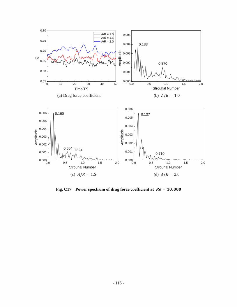
- 116 -

(a) Drag force coefficient (b)

(c) (d)

Fig. C17 Power spectrum of drag force coefficient at

0 10 20 30 40 500.55

0.60

0.65

0.70

0.75

0.80

Cd

Time(T*)

A/R = 1.0

A/R = 1.5

A/R = 2.0

0.0 0.5 1.0 1.5 2.00.000

0.001

0.002

0.003

0.004

0.005

0.870Am

plit

ude

Strouhal Number

0.183

0.0 0.5 1.0 1.5 2.00.000

0.001

0.002

0.003

0.004

0.005

0.006

0.8240.664

Am

plit

ude

Strouhal Number

0.160

0.0 0.5 1.0 1.5 2.00.000

0.001

0.002

0.003

0.004

0.005

0.006

0.710

Am

plit

ude

Strouhal Number

0.137

- 117 -

(a) Lift force coefficient (b)

(c) (d)

Fig. C18 Power spectrum of lift force coefficient at

0 10 20 30 40 50-0.15

-0.10

-0.05

0.00

0.05

0.10

0.15

Cl

Time(T*)

A/R = 1.0

A/R = 1.5

A/R = 2.0

0.0 0.5 1.0 1.5 2.00.000

0.005

0.010

0.015

0.020

0.025

0.030

Am

plit

ude

Strouhal Number

0.159

0.0 0.5 1.0 1.5 2.00.000

0.005

0.010

0.015

0.020

0.025

0.030

Am

plit

ude

Strouhal Number

0.139

0.0 0.5 1.0 1.5 2.00.000

0.005

0.010

0.015

0.020

0.025

0.030

Am

plit

ude

Strouhal Number

0.137

- 118 -

(a) Side force coefficient (b)

(c) (d)

Fig. C19 Power spectrum of side force coefficient at

0 10 20 30 40 50-0.10

-0.05

0.00

0.05

0.10

Cs

Time(T*)

A/R = 1.0

A/R = 1.5

A/R = 2.0

0.0 0.5 1.0 1.5 2.00.000

0.005

0.010

0.015

0.020

0.025

0.030

Am

plit

ude

Strouhal Number

0.160

0.0 0.5 1.0 1.5 2.00.000

0.005

0.010

0.015

0.020

0.025

0.030

Am

plit

ude

Strouhal Number

0.119

0.0 0.5 1.0 1.5 2.00.000

0.005

0.010

0.015

0.020

0.025

0.030

Am

plit

ude

Strouhal Number

0.092

- 119 -

(a)

(b)

(c)

Fig. C20 Vortex structure (side view and top view) at

- 120 -

INTERACTIONS

1. M.S. Kim and J.W. Kim, Effect of Reynolds Numbers and Aspect Ratio of Geometry on the Unsteady

Flow Physics around a Rectangular Parallelepiped, 28th AIAA Applied Aerodynamics Conference, 28

June – 1 July 2010, Chicago, Illinois, AIAA 2010-4700.

2. J.W. Kim and M.S. Kim, Analysis of Unsteady Flowfield around a MAV Using Fluent, 2010 ANSYS

Korea User Conference, 9 September – 10 September 2010, GyeongJoo, Korea.

3. M.S. Kim and J.W. Kim, Numerical Study of Unsteady Flow past a Circular Cylinder, International

Conference on Intelligent Unmanned Systems, 3 November – 5 November 2010, Bali, Indonesia, ICIUS-

2010-0131.