An Investigation of Unsteady Aerodynamic Multi-axis State ...mason/Mason_f/PedroJDeONPhD.pdf · An...
145
An Investigation of Unsteady Aerodynamic Multi-axis State-Space Formulations as a Tool for Wing Rock Representation Pedro Jose de Oliveira Neto Dissertation submitted to the Faculty of the Virginia Polytechnic Institute and State University in partial fulfillment of the requirements for the degree of Doctor of Philosophy In Aerospace Engineering Dr. William H. Mason, Advisor, Chair Dr. Eugene M. Cliff Dr. Wayne C. Durham Dr. Christopher D. Hall Dr. Craig Woolsey August 2007 Blacksburg, Virginia Keywords: High Angle of Attack, Nonlinear Dynamics, Stability Derivatives, Unsteady Aerodynamics, Wing Rock Copyright © 2007, Pedro J. de Oliveira Neto
-
Upload
truongminh -
Category
Documents
-
view
222 -
download
0
Transcript of An Investigation of Unsteady Aerodynamic Multi-axis State ...mason/Mason_f/PedroJDeONPhD.pdf · An...

An Investigation of Unsteady Aerodynamic Multi-axis
State-Space Formulations as a Tool for Wing Rock
Representation
Pedro Jose de Oliveira Neto
Dissertation submitted to the Faculty of the Virginia Polytechnic Institute
and State University in partial fulfillment of the requirements for the degree
of
Doctor of Philosophy
In
Aerospace Engineering
Dr. William H. Mason, Advisor, Chair
Dr. Eugene M. Cliff
Dr. Wayne C. Durham
Dr. Christopher D. Hall
Dr. Craig Woolsey
August 2007
Blacksburg, Virginia
Keywords: High Angle of Attack, Nonlinear Dynamics, Stability Derivatives, Unsteady
Aerodynamics, Wing Rock
Copyright © 2007, Pedro J. de Oliveira Neto

An Investigation of Unsteady Aerodynamic Multi-axis
State-Space Formulations as a Tool for Wing Rock
Representation By
Pedro J. de Oliveira Neto
Committee Chairman: Dr. William H. Mason
Aerospace Engineering
(ABSTRACT)
The objective of the present research is to investigate unsteady aerodynamic models with
state equation representations that are valid up to the high angle of attack regime with the
purpose of evaluating them as computationally affordable models that can be used in
conjunction with the equations of motion to simulate wing rock. The unsteady
aerodynamic models with state equation representations investigated are functional
approaches to modeling aerodynamic phenomena, not directly derived from the physical
principles of the problem. They are thought to have advantages with respect to the
physical modeling methods mainly because of the lower computational cost involved in
the calculations. The unsteady aerodynamic multi-axis models with state equation
representations investigated in this report assume the decomposition of the airplane into
lifting surfaces or panels that have their particular aerodynamic force coefficients
modeled as dynamic state-space models. These coefficients are summed up to find the
total aircraft force coefficients. The products of the panel force coefficients and their
moment arms with reference to a given axis are summed up to find the global aircraft
moment coefficients. Two proposed variations of the state space representation of the
basic unsteady aerodynamic model are identified using experimental aerodynamic data
available in the open literature for slender delta wings, and tested in order to investigate
their ability to represent the wing rock phenomenon. The identifications for the second
proposed formulation are found to match the experimental data well. The simulations
revealed that even though it was constructed with scarce data, the model presented the
expected qualitative behavior and that the concept is able to simulate wing rock.

i
Acknowledgments
All that I struggled to accomplish in my academic life was also part of a tentative effort
to honor all of my former teachers. The first of them was my retired uncle Dermeval, who
taught me how to read by patiently reading comics for me. Among the others, I would
like to mention the devoted Chemistry Professor Adauto de Oliveira, my father, who was
the first person to bring the beauty of Science to my attention. Another person that I
should mention my gratitude to is schoolteacher Laudelina, my mother, who took her
own life as an example and taught me to persevere and never give up, no matter how
adverse the situation could be.
The times that I spent working on this research certainly are among the most challenging
of my life in many ways. During these tough times of my Ph.D. program, I certainly
received support from God, Who helped me through several individuals. Very important
support came from the remaining members of my family, especially from Aurea, the two
Estellas, Maria, and Priscila. They helped me in so many ways that it is impossible to list
everything here. I would like at least to thank them for always keeping my positive
attitude toward the end of this program. Fundamental support gave me the late Dr.
Frederick Lutze, my first advisor in this research. He introduced me to this problem and
gave me the initial guidelines to solve it. He also provided the grant that funded most of
my stay in Blacksburg and made it possible for me to pursue the Ph.D. program. Very
important guidelines were also given to me by my committee Chair, Dr. William Mason,
who kindly lent me his multidisciplinary experience and advised me since Dr. Lutze
passed away. I would like to thank all the committee members for the revision of this
dissertation and valuable suggestions. I shall acknowledge the excellent job that the
Graduate Program Coordinator in the Aerospace and Ocean Engineering Department,
Ms. Hannah Swiger, did when she put everything together for my final examination. My
stays in Blacksburg were possible also because of the leaves of absence granted by my
employer, the Brazilian Air Force’s Institute of Aeronautics and Space (IAE), after the
ii
kind intercessions of Lt. Col. Paulo Garcia Soares, and of Col. Olympio Achilles de Faria
Mello, Ph.D., to whom I am also indebted. Dr. Mello also helped me to get the grant that
funded the last part of this research. This grant came from the Brazilian research agency
FUNCATE, and from the IAE.

iii
To all my teachers.

iv
Contents
Acknowledgments............................................................................................. i List of Figures ................................................................................................ vi List of Symbols ............................................................................................... ix List of Tables.................................................................................................. xi 1 INTRODUCTION..................................................................................................... 1
1.1 PREVIOUS WORK IN AERODYNAMIC FUNCTIONAL MODELLING .......................... 2 1.1.1 Stability Derivatives Approach................................................................... 5 1.1.2 Indicial Approach ....................................................................................... 6 1.1.3 State-Space Representation – The First Ideas ............................................ 7 1.1.4 Nonlinear Internal State Equation Model................................................. 12 1.1.5 State-Space Representation – One More Idea.......................................... 16 1.1.6 Aircraft Multi-Axis State-Space Formulation........................................... 20
1.2 THE WING ROCK PHENOMENON ........................................................................ 28 1.2.1 The Energy Exchange Concept................................................................. 34 1.2.2 Experimental Investigations on the Slender Delta Wings......................... 39 1.2.3 Analytical and Computational Investigations on the Wing Rock ............. 45
1.3 OVERVIEW OF THE THESIS ................................................................................. 47
2 THE INVESTIGATED UNSTEADY AERODYNAMIC MODELS................. 52
2.1 THE FIRST UNSTEADY AERODYNAMIC MODEL INVESTIGATED ......................... 53 2.2 THE SECOND UNSTEADY AERODYNAMIC MODEL INVESTIGATED ..................... 59
3 MODEL PARAMETERS IDENTIFICATIONS................................................. 70
3.1 PARAMETER IDENTIFICATION METHOD ............................................................. 70 3.2 SIMULATED EXPERIMENTAL DATA USED IN PARAMETER IDENTIFICATION ....... 72 3.3 IDENTIFICATION RESULTS.................................................................................. 74
3.3.1 Parameter Identification for the First Investigated Model....................... 74 3.3.2 Parameter Identification for the Second Investigated Model ................... 86
4 NUMERICAL SIMULATIONS IN ROLL ........................................................ 108
4.1 RIGID BODY DYNAMICS................................................................................... 108 4.2 COMPLETE DYNAMIC SYSTEM ......................................................................... 109 4.3 RESULTS OF THE SIMULATIONS........................................................................ 111
5 CONCLUSIONS ................................................................................................... 120
REFERENCES.............................................................................................................. 122
APPENDICES............................................................................................................... 129 APPENDIX A................................................................................................................. 129
A.1 The Convolution Integral Theorem .................................................................. 129 A.2 Angle of attack and sideslip variation during rolling motion at fixed pitch angle................................................................................................................................. 130

v
VITA............................................................................................................................... 132

vi
List of Figures
Figure 1-1 Internal state space variable in predominantly two-dimensional flows. ........... 8 Figure 1-2 Internal state-space variable in predominantly vortical flows. ......................... 9 Figure 1-3 Influence of the parameters and *α σ in the sigmoid shape for the cases
where (a) ξ = -1; (b) ξ = 1. ........................................................................................ 15 Figure 1-4 Example of the internal state equation driving function. ................................ 18 Figure 1-5 Experimental and model responses static pitching moment for a rectangular
wing with NACA 0018 airfoil. Experimental data were taken from [31]. ............... 20 Figure 1-6 Experimental and predicted CN responses for large amplitude pitch oscillations
of a rectangular wing with NACA 0018 airfoil. Experimental data were taken from [31]............................................................................................................................ 22
Figure 1-7 Crossflow streamlines and pressure distribution (dot line) for zero roll angle and positive roll rate. Figure reproduced from [46] with permission of the author.. 32
Figure 1-8 Crossflow streamlines and pressure distribution (dot line) for zero roll angle and negative roll rate. Figure reproduced from [46] with permission of the author. 33
Figure 1-9 Conceptual drawings of the rolling moment coefficient versus roll angle. Figure reprinted from [52] by permission of the author. .......................................... 36
Figure 1-10 Roll angle time-history for wing pitch angle where there is no wing rock. Figure reprinted from [46] by permission of the author. .......................................... 37
Figure 1-11 Rolling moment coefficient vs. roll angle cycle for a wing pitch angle where there is no wing rock. Figure reprinted from [46] by permission of the author. ...... 37
Figure 1-12 Time history of wing rock buildup in free to roll tests at wing pitch angle equal 30 deg. Figure reproduced from [46] by permission of the author. ................ 38
Figure 1-13 Rolling moment coefficient for a cycle of wing rock buildup. Figure reproduced from [46] by permission of the author. .................................................. 38
Figure 1-14 Rolling moment coefficient for a steady state cycle of wing rock. Figure reprinted from [46] by permission of the author....................................................... 39
Figure 1-15 Cl vs. roll angle histogram for one cycle of wing rock at θ0 = 27 degree . Data extracted from [45]. .................................................................................................. 41
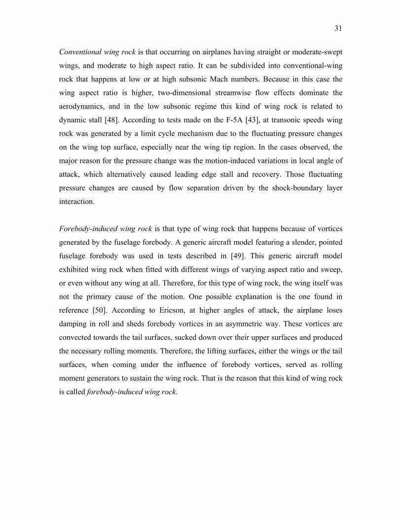
Figure 1-16 Cl vs. roll angle histogram for one cycle of wing rock at θ0 = 32 degree. Data extracted from [45]. .................................................................................................. 42
Figure 1-17 Normal force coefficient in balance coordinates vs. pitch angle – results from static tests. Data extracted from [47]. ....................................................................... 42
Figure 1-18 Rolling moment vs. pitch angle – results from static tests. Data extracted from [47]. .................................................................................................................. 43
Figure 1-19 Vertical and spanwise vortex positions during wing rock. Data extracted from [46]. (a) Vertical position. (b) Spanwise position. ........................................... 48
Figure 1-20 Sketch of asymmetric vortex position – rear view. Figure reprinted from [46] by permission of the author....................................................................................... 49
Figure 1-21 Free to roll apparatus used by Nguyen, Yip, and Chambers. Figure reprinted from [45] by permission of the American Institute of Aeronautics and Astronautics, Inc. ............................................................................................................................ 50

vii
Figure 1-22 Free to roll apparatus used by Levin and Katz [47]. Figure reprinted by permission of the American Institute of Aeronautics and Astronautics, Inc. ........... 51
Figure 2-1 Roll coeficient versus sideslip angle for the F-18........................................... 54 Figure 2-2 Static model responses vs experimental data for the normal force of the
slender delta wing, static values in balance coordinates for the improved Stagg’s model......................................................................................................................... 67
Figure 2-3 Model responses vs experimental data for the rolling moment coefficient of the slender delta wing, static values for the improved Stagg’s model...................... 68
Figure 2-4 Variation of the normal force non-dimensional arms with the roll angle, static values for the improved Stagg’s model. ................................................................... 69
Figure 3-1 Static normal force coefficient in balance coordinates vs sting pitch angle. Model responses (lines) and experimental data (geometric figures) for the improved Stagg’s model – the first investigated model............................................................ 77
Figure 3-2 Static experimental values of the rolling moment coefficients (geometric figures) and model responses (lines) vs. wing pitch angle for the first investigated model......................................................................................................................... 78
Figure 3-3 Identified static values of the normal forces non-dimensional arms vs. the roll angles for the first investigated model ...................................................................... 79
Figure 3-4 Rolling moment coefficient time histories for the first investigated model at θ0 = 20 deg. ................................................................................................................... 80
Figure 3-5 Rolling moment coefficient vs. roll angle for the first investigated model at θ0 = 20 deg. ................................................................................................................... 81
Figure 3-6 Rolling moment coefficient time histories for the first investigated model at θ0 = 27 deg. ................................................................................................................... 82
Figure 3-7 Rolling moment coefficient vs. roll angle for the first investigated model at θ0 = 27 deg. ................................................................................................................... 83
Figure 3-8 Rolling moment coefficient time histories for the first investigated model at θ0 = 45 deg. ................................................................................................................... 84
Figure 3-9 Rolling moment coefficient vs. roll angle for the first investigated model at θ0 = 45 deg. ................................................................................................................... 85
Figure 3-10 Roll angle time history for θ0 = 20 deg (above), and corresponding angle of attack time history for each half-wing (below)......................................................... 88
Figure 3-11 Rolling moment coefficient time-history at θ0 = 20 deg, second investigated model......................................................................................................................... 89
Figure 3-12 Rolling moment coefficient vs. roll angle loops at θ0 = 20 deg, second investigated model. ................................................................................................... 90
Figure 3-13 Roll angle time history for θ0 = 27 deg (above), and corresponding angle of attack time history for each half-wing (below)......................................................... 91
Figure 3-14 Rolling moment coefficient time-history at θ0 = 27 deg, second investigated model......................................................................................................................... 92
Figure 3-15 Rolling moment coefficient vs. roll angle loops at θ0 = 27 deg.................... 93 Figure 3-16 Roll angle time history for θ0 = 38 deg (above), and corresponding angle of
attack time history for each half-wing (below)......................................................... 94 Figure 3-17 Rolling moment coefficient time-history at θ0 = 38 deg............................... 95 Figure 3-18 Rolling moment coefficient vs. roll angle loops at θ0 = 38 deg.................... 96

viii
Figure 3-19 Roll angle time history for θ0 = 45 deg (above), and corresponding angle of attack time history for each half-wing (below)......................................................... 97
Figure 3-20 Rolling moment coefficient time-history at θ0 = 45 deg............................... 98 Figure 3-21 Rolling moment coefficient vs. roll angle loops at θ0 = 45 deg.................... 99 Figure 3-22 Time histories at θ0 = 27 deg of the internal state variables related to the
spanwise and vertical positions of the vortices cores. ............................................ 100 Figure 4-1 Free to roll simulations at wing pitch angle equal 30 deg, starting at roll angle
equal 5 degree. ........................................................................................................ 112 Figure 4-2 Phase-plane of the simulation response at pitch angle equal 30 deg, initial roll
angle of 5 degree..................................................................................................... 113 Figure 4-3 Free to roll simulations at wing pitch angle equal 30 deg, starting at roll angle
equal -5 degree........................................................................................................ 114 Figure 4-4 Phase-plane of the simulation response at pitch angle equal 30 deg, initial roll
angle of -5 degree.................................................................................................... 115 Figure 4-5 Free to roll simulations at wing pitch angle equal 30 deg, starting at roll angle
equal -12 degree...................................................................................................... 116 Figure 4-6 Phase-plane of the simulation response at pitch angle equal 30 deg, initial roll
angle of -12 degree.................................................................................................. 117 Figure 4-7 Free to roll simulations at wing pitch angle equal 25 deg, starting at roll angle
equal -10 degree...................................................................................................... 118 Figure 4-8 Phase-plane of the simulation response at pitch angle equal 25 deg, initial roll
angle of -10 degree.................................................................................................. 119

ix
List of Symbols
Latin Alphabet
ai, bi, ci coefficients of the quadratic polynomials that represent the stability
derivatives in function of the internal state variables.
b wing span.
CN normal force coefficient.
Cl rolling moment coefficient
maxLC maximum lift coefficient
D switching function for the right hand side of the internal state equations. It
assumes value 0 when the airplane motion variable is going up, and 1
when is going down. It also stands for drag force.
Ixx, Iyy, Izz airplane moments of inertia with respect to the body axes
Ixy, Ixz, Iyz airplane products of inertia with respect to the body axes
L, M, N components of the airplane aerodynamic resulting moment along body
axes. L also stands for lift force.
p, q, r components of the airplane angular velocity vector along body axes.
q , dynamic pressure of the undisturbed flowfield. ∞q
u, v, w components of the airplane linear velocity vector along body axes.
U switching function for the right hand side of the internal state equations. It
assumes value 1 when the airplane motion variable is going up, 0 when is
going down.
V, VT airspeed of the undisturbed flowfield.
X, Y, Z components of the airplane aerodynamic resulting force along body axes.
x internal state variable that represents the non-dimensional distance from
the trailing edge to either the position of the separation point or the
position of the vortex breakdown, measured from the trailing edge and
divided by the chord.

x
( )α0x static dependence function between the position of the point where the
flow separates and the angle of attack.
y internal state variable related to the non-dimensional spanwise position of
the leading edge vortex core.
( )φ0y function that represents the static dependence function between the
spanwise position of the leading edge vortex core and the roll angle.
t̂ convective time
Greek Alphabet
α angle of attack ∗α angle of attack value at which the separation reaches half of the chord, and
used to position the logistic function that represents the static dependence
of the separation point coordinate with the angle of attack.
β sideslip angle
θ pitch angle
v internal state variable related to both the vortex core vertical position and
vortex strength.
( )φ0v function that represents the static dependence between the internal state
variable v and the roll angle.
φ roll angle ∗φ roll angle value that gives the position of the logistic function that
represents the static dependence of either the vortex core spanwise
position or the combination of vertical position and vortex strength.
σ slope of the logistic function
1τ transient time of flow adjustment
2τ time-delay for flow adjustment
ξ airplane side of the lifting surface panel considered.
ψ head angle

xi
List of Tables
Table 1-1 Geometrical and physical parameters of some tested slender delta wings....... 49 Table 3-1 Model parameters for the first investigated model......................................... 101 Table 3-2 Model parameters for the second investigated model. ................................... 102 Table 3-3 Continuation of Table 3-2 ............................................................................ 103 Table 3-4 Parameters related to the internal state driving equation location and slope in
function of the roll angle for the first investigated model. ..................................... 103 Table 3-5 Identified values of the second investigated model parameters stored as xCN 104 Table 3-6 Continuation of Table 3-5. ............................................................................. 105 Table 3-7 Identified values of the second investigated model parameters stored as xCl. 105 Table 3-8 Identified values of the second investigated model parameters stored as xdyn 106 Table 3-9 Continuation of Table 3-8 .............................................................................. 107

1
1 Introduction
The atmospheric flight dynamics study of a vehicle is the study of the interaction of the
equations of motion and the equations of the airflow around the vehicle. The equations of
motion are given by Newton’s laws and depend on the forces and moments acting on the
vehicle. Among these forces are the aerodynamic ones that are functions of the airflow
around the vehicle, which in turn depend on the previous motion history. The
aerodynamic forces can be fully described by a set of nonlinear partial differential
equations known as the Navier-Stokes equations. At the present time computational
methodology and computer power are not adequate to provide time accurate solutions to
the Navier-Stokes equations in the flight dynamics simulation environment. Even if the
methodology existed, the cost of the computations would be very high. Recently,
computational fluid dynamics methods based on Navier-Stokes equations have been
increasingly used to predict control and stability derivatives in the early phase of the
aircraft design, but a lot has yet to be done [1]. For this reason, more practical and
simpler methods for the determination of the aerodynamic forces that could be used in
conjunction with the equations of motion have been constantly sought. These methods
can be divided into physical and functional modeling methods. Physical modeling
methods for the aerodynamic forces are those directly derived from the very first physical
principles. One example of a physical method is the unsteady vortex lattice method and
its reduced order model [2]. The physical methods may have the advantage of not being
derived from test data, but they usually are too computationally expensive for use either
in simulation or in global stability analysis. The functional modeling methods are those
that use mathematical expressions or equations to reproduce input/output response. In this
work, we evaluate functional modeling methods that in previous research have shown the
ability to reproduce the dynamic behavior of unsteady aerodynamics in longitudinal
motion.

2
The conventional quasi-steady functional modeling techniques – the idea of making the
equations linear by taking Taylor series expansion of the aerodynamic forces in terms of
the vehicular velocity, angular rates, and their derivatives with respect to time - has been
used for most flight dynamics studies since 1911 [3]. For the years that followed, the
aerodynamic functions were approximated by linear expressions leading to a concept of
stability and control derivatives. As modern fighters reached high angles of attack and
performed maneuvers at high angular rates, the linearized methods became insufficiently
accurate for analysis. The addition of nonlinear terms, expressing, for example, changes
in stability derivatives with the angle of attack, extended the range of flight conditions to
high-angle-of-attack regions and/or high-amplitude maneuvers. In both approaches, using
either linear or nonlinear aerodynamics, it is assumed that the parameters appearing in
polynomial or spline approximations are time invariant. However, high-performance
fighters have the capability to operate not only at high angles-of-attack but also with high
angular rates, situations where severely separated flow conditions prevail. Under these
conditions, the aerodynamic loads may be not only highly nonlinear but also time
dependent. We shall remember that future combat air vehicles will probably be
uninhabited. Without the pilot’s physiological limitations, they will be capable of
performing more agile maneuvers, also will take advantage of dynamic lift, and
experience higher load factors, thus increasing the importance of capturing nonlinear
unsteady aerodynamic phenomena and performing nonlinear stability analyses.
Some of the functional models that have been previously proposed to simulate unsteady
aerodynamic behavior are described in this chapter. Also reviewed is the previous work
done in the research of the phenomenon called wing rock.
1.1 Previous Work in Aerodynamic Functional Modelling
Bryan [3], who published the first complete analysis of the pitch stability of an aircraft at
the very beginning of heavier-than-air flight, was probably the first to introduce modeling
of the aerodynamic forces acting on the aircraft, and his model was linear. Since then, the
idea of making the equations linear by taking Taylor series expansions of the

3
aerodynamic forces in terms of the vehicular velocity, aerodynamic angles, angular rates,
and their time-derivatives has been used for most flight conditions. The linear terms
associated with these expansions are known as aerodynamic stability derivatives [4] and
an important fraction of the total effort in aerodynamic research in the past has been
dedicated to find a methodology for their determination, by theoretical, semi-empirical
and experimental means. The range of usefulness of this method can be extended to
higher angles of attack by adding higher order nonlinear terms. However, the parameters
appearing in conventional applications are assumed to be time-invariant.
This time-invariance does not correspond to results of studies in unsteady aerodynamics
that started in the nineteen-twenties with Wagner [5]. He studied the unsteady lift on an
airfoil due to abrupt changes in the angle of attack. His work was extended by
Theodorsen [6] to compute forces and moments on an oscillating airfoil, whereas
Kussner [7] studied the lift on an airfoil as it penetrates a sharp-edge gust. Cicala [8] and
Jones [9] started to investigate the unsteady aerodynamics of finite wings.
The concern with modeling the unsteady aerodynamic effects is present in other works of
Jones [9]-[12], who introduced the concept of the indicial functions approach. In [12], he
extended the work in unsteady aerodynamics from wings to airplanes, by studying the
effect of the wing wake on the lift of the horizontal tail. The formulation of linear,
unsteady aerodynamics in the aircraft longitudinal equations in terms of indicial functions
was further developed by Tobak in [13]. Later, in [14]-[17], Tobak et al expressed the
longitudinal aerodynamic forces and moment as functionals of the angle of attack and the
dimensionless pitch angular rate, free of the dependence on a linearity assumption. The
indicial functions approach is considered the most systematic and rigorous functional
way of representing unsteady aerodynamics, and it is currently applied [18]-
[21],[22],[23],[24], but it is more difficult to combine this functional representation with
the equations of an aircraft motion, which are written in the form of differential
equations.

4
A nonlinear, lifting line procedure with unsteady wake effects was developed and studied
for predicting wing-body aerodynamic characteristics up to and beyond stall by Levinsky
[25] and Hreha [26]. In this nonlinear lifting line formulation, a discrete vortex lattice
representation is used for the time-dependent wake, whereas the wing load distribution is
assumed concentrated along the 25% chord line. Each chordwise section is assumed to
act aerodynamically (including stall) like a 2D airfoil in steady flow at effective angle of
attack, which may also be time dependent. Three-dimensional unsteady aerodynamic
effects were included by allowing shed vortices in the wake to vary in strength with
distance and time. The strengths of the shed vortices are related to those of the
corresponding bound elements at an earlier time, based on the convective time delay at
free stream velocity between the bound vortex and the particular wake station. Although
the theory is unsteady from the point of view of wake-induced effects, it is assumed that
the two-dimensional airfoil chordwise loadings and sectional characteristics in stall are
steady state. The method is also limited to incompressible flow, and to wings of moderate
sweep and from moderate to large aspect ratio. Some further applications of this
formulation are shown in [27].
A functional approach to include unsteady aerodynamics in aircraft equations of motion
was introduced by Goman et al in [28],[29], which consisted of a state-space
representation of additional internal state variables that are used in the functional
relationships for the aerodynamic forces and moments. Fan and Lutze [30] took their idea
and combined it with the idea of extending the range of applicability to higher angles of
attack by adding higher order nonlinear terms in the Taylor’s series expansion. In
addition to that, they defined the aerodynamic coefficients and derivatives as quadratic
polynomials of an internal state variable related to the flow separation point position. The
state-space representation is convenient for solving problems of flight dynamics because
the inclusion of unsteady aerodynamics in the above form leads only to an increase in
problem dimension and retains the possibility of investigating motion stability by means
of classical methods. Nevertheless, this model, as it was originally proposed, is not
capable of simulating multi-valued aerodynamic characteristics for quasi-static motion
(static hysteresis). Later, Abramov, Goman, Khrabrov, and Kolinko [31] presented
5
another state-space representation of aerodynamic characteristics that included nonlinear
terms and that was capable of describing static hysteresis. An additional state-space
approach that could do this with fewer model parameters is the one presented by De
Oliveira and Lutze [32].
Next, some functional unsteady aerodynamic models of more interest, selected among the
ones mentioned before, are described in more detail.
1.1.1 Stability Derivatives Approach
In this method, the problem of airplane dynamics is formulated and the equations for six-
degree-of-freedom motion are derived through Newton’s laws. Because these equations
are coupled and nonlinear, it is difficult to obtain analytical solutions. In view of this, it is
assumed that the motion following a disturbance has small amplitudes in all the disturbed
variables. With this assumption, it is possible to linearize the equations of motion about
the chosen flight condition. If the airplane configuration allows the definition of a vertical
plane of symmetry, it is possible to decouple the equations of motion into two sets: one
for the longitudinal motion and another for lateral-directional motion. Nevertheless, there
are cases where the decoupling is not possible, like for example, those whose mass
distribution is not symmetric. Even in such cases, the linear equations of motion can be
used in the stability analysis [33]. After linearization, it is assumed that the aerodynamic
forces and moments in the disturbed state depend only on the instantaneous values of
motion variables. This allows them to be evaluated by using the method of Taylor series
expansion. With these approximations, the equations of motion become linear in all the
motion variables. The aerodynamic coefficients appearing in the Taylor series expansion
are called stability and control derivatives.
For flight conditions where massively separated flow conditions prevail, the linearized
methods become insufficiently accurate for the analysis and more accurate aerodynamic
models are required.

6
1.1.2 Indicial Approach
The concept of indicial aerodynamic functions may be defined briefly as “the
aerodynamic response of the airfoil as a function of time to an instantaneous change in
one of the conditions determining the aerodynamic properties of the airfoil in a steady
flow” [13]. Recent developments and applications of the indicial approach to the
representation of unsteady aerodynamics can be found in references [18], [19], and [22].
A short summary based on these references follows.
In this approach, the combined vector of the total aerodynamic coefficients
of an aircraft undergoing an arbitrary motion is the
indicial response obtained in conjunction with the superposition principle
Cr
[ TnmlLYD CCCCCC= ]
[15], [16] or
Duhamel’s integral theorem (Appendix A.1). This indicial response is given by
( )∫ −=t
dhtC0
ττ &rrA (1-1)
Where { }i
j
hCA=A is a matrix of indicial response functions for stepwise variations of
kinematic parameters and control surfaces deflections combined in the vector
. That means that, in this approach, the variations
with time of the aircraft kinematic variables such as angle of attack and angular velocity
are replaced by a large number of small instantaneous step changes. The transient
aerodynamic reactions to these step changes are named “indicial functions”, and the total
response is obtained by their superposition.
hr
[ Trearqp δδδβα= ]
Even though this approach is considered a good representation of unsteady aerodynamics,
it is difficult to combine it with the differential equations of motion. The indicial concept
was originally conceived for linear time-invariant systems, but it has been generalized to
7
a nonlinear indicial response theory [22], leading to a much more complicated
description.
1.1.3 State-Space Representation – The First Ideas
In the indicial approach, the aerodynamic coefficients are represented by integral-
differential equations, which are neither easy nor suitable to combine with the airplane
differential equations of motion. To overcome this difficulty, a state-space approach to
represent unsteady aerodynamics was proposed in 1990 [28],[29], which added internal
variables describing the state flow in the functional relationships for the aerodynamic
coefficients for forces and moments. The values of the total aerodynamic force and
moment depend on the kinematic parameters of the motion and on either the position of
the flow separation or the position of the vortex breakdown. Thus the separation point
position and the vortex burst point position were taken as internal dynamical variables in
the original formulation of this type of representation. In this approach, an internal state
variable associated with the state of the flow was used to represent the unsteady
aerodynamic effect. It can be associated either with the distance between the airfoil
trailing edge and the position of the point of separation, in predominantly two-
dimensional type of flows (
( )tx
Figure 1-1 ), or to the position along the chord of the vortex
burst point, in predominantly vortical type of flows ( Figure 1-2 ).

8
Figure 1-1 Internal state space variable in predominantly two-dimensional flows.
This internal state-space variable is then made non-dimensional by divison either by
M.A.C. ( wing mean aerodynamic chord ), in case of wings with moderate to large aspect
ratio, or by cr ( chord in the plane of symmetry ), in case of wings with low aspect ratio.
Therefore, the non-dimensional variable ( )tx associated with ( )tx is ( ) ( ) .../ CAMtxtx =
or ( ) ( ) rctxtx /= . Consequently, ( )tx [ ]1,0∈ . As shown in figures 1-1 and 1-2, the value
0=x corresponds either to attached flow or to the absence of vortex breakdown over the
wing, while 1=x corresponds to leading-edge separation or vortex burst at the apex. We
take the wing trailing edge as the origin for ( )tx because it is consistent with the second-
order polynomial model (equations (1-8)) adopted here for the stability derivatives, after
the work of Fan & Lutze [30],[34]. This is in contrast to the reference system taken by
Goman & Khrabrov [29], where the leading edge is adopted as the origin of . ( )tx

9
Figure 1-2 Internal state-space variable in predominantly vortical flows.
Taking into account the above features, a mathematical model was proposed [28],[29]
where the internal dynamical variables (vector xr ) approximately describes the state of
separated and vortex flow about an aircraft. These variables are additional information
required at a given instant of time to calculate the outputs (aerodynamic forces and
moments, given by the vector Cr
[ ]TnmlLYD CCCCCC= ) from the system
inputs (motion variables and surfaces deflections, given by the vector
). The unsteady aerodynamic state-space approach
is then given by a dynamical system
hr
[ Trearqp δδδβα= ]
(1-2)
( )hxfdtxd rrr
,=
( )hxgCrrr
,= (1-2)
To obtain the simplest mathematical model of this kind, Goman and Khrabrov [29] first
considered the flow about a wing in pitching motion only. Then, the first equation of the
dynamical system (1-2) was defined as:

10
( ) ( ) ( ) ( )( )ttxtxtx ατατ && 201 −=+ (1-3)
This definition was taken with two groups of unsteady fluid mechanics processes in
mind. The first group concerns the different quasi-steady aerodynamic effects that have
time-delays, such as circulation and boundary-layer convection lags. Since the resulting
delay is approximately proportional to the variation of the angle of attack α& , the quasi-
steady value of the internal state variable can be expressed through the function ( )α0x by
means of argument shift ( )ατα &20 −x , where 2τ defines the total time delay associated
with the above-mentioned effects. The second group of fluid mechanics processes defines
transient aerodynamic effects such as the dynamics of the flow adjustment to any change
in the angle of attack. This dynamics can be described by the first-order differential
equation (1-3), where 1τ is the transient time-constant.
The steady state position ( )α0x of the separation point is generally a nonlinear function
of the angle of attack. It can be obtained from static wind tunnel measurements, but, in
order to be applicable for identification purposes, a mathematical relation would be more
suitable.
In references [30],[34], Fan and Lutze started from the state-space model as proposed by
Goman and Khrabrov [29], and further developed it to facilitate the identification
process. Their first improvement was to propose the logistic or sigmoid function (1-4)
shown below as the representation of ( )α0x .
( )( )( )( )( )∗
Δ
−+=
αασα
ttx
effeff exp1
10
(1-4)
where ( ) ( ) ( )ttteff αταα &2−= , is the angle of attack at which the flow separation is at
the mid-chord point, and
∗α
σ is the slope factor. Parameters and ∗α σ are expected to be
identified from wind tunnel experimental data. Figure 1-3 shows the influence of these
parameters in the shape of the sigmoids for negative (a) and positive (b) values of σ .
Because in the current work the sign of σ plays such an important role for the wing rock

11
representation, we write it explicitly, as it is shown in equation (1-5), and assume that
σσ = .
( )( )( )( )( )∗−+
=ααξσ
αt
txeff
eff exp11
0 (1-5)
with =ξ -1 or +1 for sigmoid functions that respectively increase or decrease with
increasing values of α .
By considering the symmetrical motion in the longitudinal plane, the output equations
were written as functionals of the kinematic variables involved in this kind of motion,
that is,
(1-6) ( ) ( ) ( ) ( ) ( )( )txtqttCtC aa ,,,αα &=
where is the aerodynamic coefficient, like, for example, a mLDa ,,=
Since these functions are not known, practical schemes were developed [30],[34] to have
them easily identified with the help of experimental data. In order to achieve that, Taylor
series expansions of (1-6) in terms of the motion variables α and q were used, and the
terms up to second order were retained. These expansions were taken around
( 0,0 == q )α , while holding the state x fixed.
Taking the lift coefficient output equation as example (a = L), we have:
(1-7) ( ) ( ) ( ) LqLLLL CqxCxCCtC 2ˆ0 ˆ Δ+++= αα
Where represents the second-order terms, that is LC2Δ
( ) ( ) ( ) qxCqxCxCC qLqLLL ˆˆ ˆ2
ˆ22
22 αα αα ++=Δ
Here, is the nondimensional pitch rate, and tqq ˆˆ =Vct
2ˆ = is the characteristic time of
the flow, sometimes called convective time.

12
In the above equations (1-6) and (1-7), the stability derivatives are no longer constant as
in the conventional approach, but assumed as functions of the internal state variable x .
To allow for parameter identification, they were defined in references [30],[34] as
quadratic polynomials of the internal state variable x , that is,
( ) 2111 xcxbaxCL ++=α
( ) 2222ˆ xcxbaxC qL ++=
( ) 23332 xcxbaxCL ++=α (1-8)
( ) 2444ˆ 2 xcxbaxC qL ++=
( ) 2++= 555ˆ xcxbaxC qLα
Where , and , j = 1,2,…,5 are constants to be determined from experimental
data. Similar expressions were derived for drag and pitching moment coefficients
and .
ja jb jc
DC
mC
Developments made in references [18] and [22] show that, for the linear domain, the
indicial function approach is equivalent to the state-space representation.
1.1.4 Nonlinear Internal State Equation Model
The state-space approach described in the preceding section is not capable of representing
some nonlinear phenomena like, e.g., static hysteresis. In [31], Abramov et al introduced
a more comprehensive variation of this approach that is capable of making up for these
shortcomings. They developed a nonlinear model that naturally describes static hysteresis
and critical state crossings [35], by connecting them to the mathematical phenomenon
known as the Riemann-Hugoniot catastrophe [36]. Their model is built based on the
assumption that the contributions from potential or attached (pt) and separated (sp) flows
have different time scales and must be represented separately, as shown in Eq. (1-9):

13
( ) ( ) ( )tCV
cCCtC spNptNptNN ++= αα
α
&&
(1-9)
where ( )αptNC , are the static dependency and aerodynamic derivative for attached
flow. The term defines the separated flow contribution that accounts for all the
nonlinear unsteady effects. To describe the transition from an attached to a fully stalled
flow, they introduced an internal state variable,
α&ptNC
( )tC spN
10 ≤≤ x , associated with the size of the
separated region of the wing, such that
( ) ( )( ) ( ) ⎥⎦⎤
⎢⎣⎡ Δ+Δ=
VcCCtxgtC
fsfssp NNNαα
α
&&
(1-10)
where is the weight function, equal to zero for fully attached flow and to 1 for
fully separated conditions. The terms
( )( txg )( ) ( ) ( )ααα
ptfs NNfsN CCC −=Δ ,
are the aerodynamic contributions due to fully separated or stalled
(fs) conditions.
ααα &&& ptfsfs NNN CCC −=Δ
To allow the model to describe static hysteresis and critical states, the following
nonlinear dynamic equation for the internal state variable x was introduced:
( )xFdtdx ,*α=
(1-11)
where ( ) ( ) ( ) ( ) 3*3
2*2*1*0 xkxkxkkF αααα +++= and
Vck ααα α&
&−=* . This third order
polynomial defined as the right hand side of Eq. (1-11) allows the representation of the
two stable branches in static hysteresis. Since each set of coefficients
( ) ( ) ( ) ( )*3*2*1*0 ,,, αααα kkkk define a different set of equilibrium points
( ){ 0, s.t. =ee xFx }α for each angle of attack, the model can represent flows with one or
two stable branches, being able of naturally identify models with static hysteresis.
When this model is used for parameter identification, we can see that it is necessary to
identify one set of coefficients ( ) ( ) ( ) ( )*3*2*1*0 ,,, αααα kkkk for each angle of attack

14
chosen for the calculations, and this can make the number of required parameters too
large to be identified.

15
(a)
(b)
Figure 1-3 Influence of the parameters and *α σ in the sigmoid shape for the cases where (a) ξ = -1; (b) ξ = 1.
16
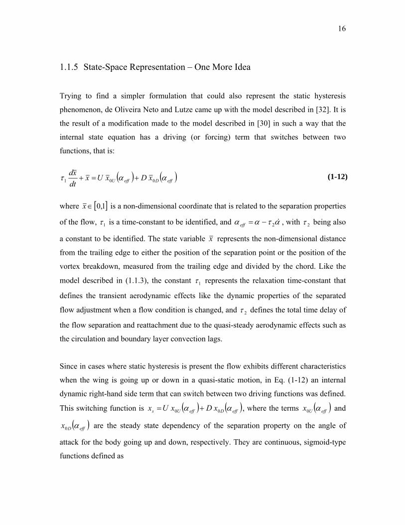
1.1.5 State-Space Representation – One More Idea
Trying to find a simpler formulation that could also represent the static hysteresis
phenomenon, de Oliveira Neto and Lutze came up with the model described in [32]. It is
the result of a modification made to the model described in [30] in such a way that the
internal state equation has a driving (or forcing) term that switches between two
functions, that is:
( ) ( )effDeffU xDxUxdtxd αατ 001 +=+ (1-12)
where [ ]1,0∈x is a non-dimensional coordinate that is related to the separation properties
of the flow, 1τ is a time-constant to be identified, and αταα &2−=eff , with 2τ being also
a constant to be identified. The state variable x represents the non-dimensional distance
from the trailing edge to either the position of the separation point or the position of the
vortex breakdown, measured from the trailing edge and divided by the chord. Like the
model described in (1.1.3), the constant 1τ represents the relaxation time-constant that
defines the transient aerodynamic effects like the dynamic properties of the separated
flow adjustment when a flow condition is changed, and 2τ defines the total time delay of
the flow separation and reattachment due to the quasi-steady aerodynamic effects such as
the circulation and boundary layer convection lags.
Since in cases where static hysteresis is present the flow exhibits different characteristics
when the wing is going up or down in a quasi-static motion, in Eq. (1-12) an internal
dynamic right-hand side term that can switch between two driving functions was defined.
This switching function is ( ) ( )effDeffUs xDxUx αα 00 += , where the terms ( )effUx α0 and
( )effDx α0 are the steady state dependency of the separation property on the angle of
attack for the body going up and down, respectively. They are continuous, sigmoid-type
functions defined as

17
( ) ( )[ ]∗−−+=
UeffUeffUx
αασα
exp11
0 (1-13)
( ) ( )[ ]∗−−+=
DeffDeffDx
αασα
exp101
(1-14)
where is the angle of attack at which the flow separation or the vortex burst position
is at the mid-chord point, and
( )∗•α
( )•σ is the slope factor. An example of the flow separation
functions for up and down motions with the parameters ( deg, 15.7=∗Uα ,deg 20.1=∗
Dα
,31.7=Uσ )14.5=Dσ is shown in Figure 1-4. We can observe in this figure the
influence of ( )•Sα and ( )•σ on the shape of the sigmoids. The parameters U and D on the
right-hand side of Eq. (1-12) are respectively defined as
( )2
1 αΔ+=Δ signU
(1-15) ( )2
1 αΔ−Δ sign=D
where ii ααα −=Δ +1 for the given sequence of the static angles of attack iα , i = 1,2,…,l
correspond to the wind tunnel measurements of the aerodynamic coefficients
( ){ }liC ia ,...,2,1,ˆ =α , and where ( ) ( )ii tt ααα −=Δ +1 for the given time histories of
angles of attack ( ){ nii ttt ≤≤0, }α correspond to the wind tunnel measurements of the
aerodynamic coefficient time histories ( ){ }nitC ia ,...,2,1,ˆ = . The subscript a represents
the type of coefficient being modeled, for example a = D, L or m.

18
0 5 10 15 20 25 30 35 40 45 500
0.2
0.4
0.6
0.8
1
α , deg
xdriving
Up Down
Figure 1-4 Example of the internal state equation driving function.
The output equations for the aerodynamic coefficients are defined to be functions of the
internal state ( )tx , the angle of attack ( )tα , the pitch rate ( )tq , and are, as in [34], written
in the following form:
( ) ( ) aqaaaa CqxCxCCC 2ˆ0 ˆ Δ+++= αα (1-16)
with
( ) ( ) ( ) qxCqxCxCC qaqaaa ˆˆ ˆ2
ˆ22
22 αα αα ++=ΔΔ
being the nonlinear part of the equation, where a represents the aerodynamic coefficient
modeled.
tqq ˆˆ = is the non-dimensional pitch rate and t is the characteristic time of the flow,
defined as
ˆ

19
Vct
2ˆ = , (1-17)
c being a characteristic length, and V the airspeed. It is worthwhile noting that the
convective time Vc is related to the time it takes for an air molecule to travel along the
wing mean aerodynamic chord. The factor ½ is included in Eq. (1-17) because it was
used to determine the non-dimensional pitch rate in most of the references related to
unsteady aerodynamics and flight dynamics. The reason for that is probably just tradition.
The mid-chord was historically taken as the coordinate origin for a pitching airfoil in
unsteady aerodynamics analysis and, as a natural consequence, the semi-chord was
introduced as the characteristic length [37],[38].
The stability derivatives in Eq. (1-16) are defined as quadratic polynomials of the non-
dimensional state variable x , that is
2)( xcxbaxC aaaa χχχχ ++= ,
where a is the type of aerodynamic coefficient, and χ represents the motion variables
with respect to which the partial derivatives were taken. In this case, =χ qqq ˆ,ˆ,,ˆ, 22 ααα .
In [32] this formulation was used to represent the static hysteresis of an NACA 0018
airfoil, reported in [31]. The comparison between wind tunnel data and model responses
for pitching moment and normal force coefficients can be seen in Figure 1-5 and Figure
1-6, respectively. They show that this formulation matches very well experimental
results.

20
Figure 1-5 Experimental and model responses static pitching moment for a
rectangular wing with NACA 0018 airfoil. Experimental data were taken from [31].
1.1.6 Aircraft Multi-Axis State-Space Formulation
The method presented in the section 1.1.5 can be used to represent only symmetrical
longitudinal motion of wings and airplanes. Trying to find some formulation that could
represent more general types of motion, we composed this method with the formulation
originally described by Lutze, Fan and Stagg in [39] and [40] to build the models that
have the ability to represent wing rock investigated in their research. This later
formulation is briefly reproduced in this section for the convenience of the reader. The
primary idea behind this method is the decomposition of the aircraft into several elements
that contribute to the resulting aerodynamic force. These elements are small lifting
surfaces that are referred to as panels. The approach taken is one of modeling the local
forces and moments associated with the contributing lifting surfaces of the aircraft such
as left and right wings, left and right horizontal tails, vertical tail, and surfaces

21
representing forward and aft fuselage. When an airplane rotates in the air, the air velocity
is different at each surface, making the local angles of attack also different. Since the
state-space model is based upon characterizing flow separation as a function of angle of
attack, the work in this model is done using the local angle of attack and its time
derivative. The local forces and moments can be calculated on each panel and, when
combined with the forces and moments on the remaining panels, the total forces and
moments for the whole aircraft are obtained. The goal is not only to characterize the
rolling moment, but also the forces and moments along and about the other axes. The
idea is to have one model capable of the prediction of lateral/directional characteristics as
well as the longitudinal ones, even in the high angle of attack, unsteady aerodynamic
region.
Next, the description of the basic model for each of the single lifting surfaces in this
formulation is reproduced with its original notation.
► Normal Force on Left and Right Wings
The aerodynamic normal force acting on the left and right wing is represented in this
model by the following state-space formulation [30],[34],[39],[40] :
( )wiwwiwwiwi
w xxdt
dx ατατ &201 −=+ (1-18)
( ) ( )xCxCCC wiwiiNwwiwiiNwiNwNwi α αα &0 α&++=
where subscript “w” represents quantities of the wing or the forward group of lifting
surfaces, and i = l or r, respectively, standing for the left or right panel. In the state
equation of (1-18) 1wτ is the wing panel relaxation time constant defining the transient
aerodynamic effects and 2wτ quantifies the time delay due to the quasi-steady
aerodynamic effects about the wing panel. The variable is the wing panel state
variable associated with the nonlinear flow effects, and
wix
( )wiwx α0 is the static dependency

22
of the state variable on the local angle of attack, given by the sigmoid-type function
defined by
( ) ( )( )wwiwwiwx ∗−−+
=αασ
αexp1
10 (1-19)
Figure 1-6 Experimental and predicted CN responses for large amplitude pitch
oscillations of a rectangular wing with NACA 0018 airfoil. Experimental data were
taken from [31]

23
In equation (1-19) describes the location of this function, ∗wα wσ is the slope factor, and
wiα is the local angle of attack of the wing panel at a location along the wing span at a
distance from the axis of the fuselage. In this work the primary concern is with pure
rolling oscillatory motions. For this kind of motion the local velocity components at that
location can be expressed in the body-axis system as (see Appendix A.2),
wl
0cosθTw Vu =
(1-20) θ φsinsinVv =
&
Tw 0
φφθ m wTw lsinVw cos0=
where the negative sign corresponds to the left wing panel while the plus sign to the right
wing panel. The angle of attack and the sideslip angle are defined as,
uw1tan −=α
(1-21)
222
1
wvusin
++= −β v
Subtituting (1-20) into (1-21), the local angle of attack values for the left and right wing
panels can be calculated through
⎟⎟⎠
⎞⎜⎜⎝
⎛−= −
00
1
coscostantan
θφφθα
T
wwl V
l &
(1-22) ⎟⎟⎠
⎞⎜⎜⎝
⎛+= −
00
1
coscostantan
θφφθα
T
wwr V
l &
The output of the system (1-18) is , the normal force coefficient on the left or right
wing panel. The derivatives
iNwC
( )wiiNw xC α and ( )wiiNw xC α& are modeled as,

24
( ) 21111 wiwiwwwiiNw xcxbaxC ++=α
(1-23) ( ) 2222 wiwwiwwwiiNw xcxbaxC ++=α&
where , , and are constants to be identified from experimental results. wja wjb wjc
► Normal Force on Left and Right Horizontal Tails
The horizontal tail is modeled in a similar way to the wing, by
( )tittittiti
t xxdt
dx ατατ &201 −=+
( ) (( ))*20 exp1 ttittitititx
αασατα
−−+=− &
1
( )
(1-24)
( ) ( )2titiNtititiNtititiNtiNtiNti xCxCxCCC ααα ααα &
&+++= 0 2
Subscript “t” stands for horizontal tail, and the left and right horizontal tails are
represented respectively by i = l, r.
Not considering the aerodynamic interference from the wing, the local angle of attack at
the left and right horizontal tail panels is written as,
⎟⎟⎠
⎞⎜⎜⎝
⎛−= −
00
1
coscostantan
θφφθα
T
tlt V
l &
(1-25)
⎟⎟⎠
⎞⎜⎜⎝
⎛+= −
00
1
coscostantan
θφφθα
T
trt V
l &
where lt is the distance of the selected location on the horizontal tail panel from the
aircraft longitudinal axis, also another parameter to be identified.
The aerodynamic derivatives in Eq. (1-24) are, like the wing, modeled by quadratic
polynomials of the internal flow state variable as

25
( ) 2111 tittitttiNti xcxbaxC ++=α
( ) 2
( ) 2
2222 tittitttiNti xcxbxC ++=αα (1-26)
333 tittitttiNti xcxbxC ++= αα&
► Side Force on Vertical Tail
The sideslip angle values were relatively small in the wind-tunnel tests reported in Refs.
[39], [40]. Because of that, the classic stability derivative approach was used to model the
aerodynamic side force acting on the vertical tail, that is,
vYtvYtvY CCC ββ ββ&
&+= (1-27)
Where and are constant parameters. In Eq. βYtC β&YtC (1-27), vβ and are,
respectively, local sideslip angle and its time-derivative at a selected location on the
vertical tail. The distance of this location from the longitudinal body axis is represented
by parameter . For the pure rolling oscillatory motion,
vβ&
3l vβ can be obtained as
⎟⎟⎠
⎞⎜⎜⎝
⎛+= −
Tv V
lsinsinsin φφθβ&
30
1
(1-28)
In case of larger values of the sideslip angle, parameters and could also be
defined as quadratic polynomials of some local, internal flow state variable.
βYvC β&YvC
► Side Force on the Fuselage
In this formulation, the only fuselage contribution to appear explicitly is that related to
the lateral force. The fuselage contribution to the normal force is assumed to be lumped
into those from the wing and the horizontal tail. For the same reason as in the case of the
vertical tail, the side force acting on the fuselage is modeled as,

26
(1-29) ββ ββ&
&YbYbbY CCC +=
where β and are, respectively, the aircraft sideslip angle and its time-derivative. β&
The panel contributions are then summed up in an appropriate way to give the
approximate aerodynamic characteristics of the whole aircraft, as shown below for a
conventional airplane configuration.
► Normal Force Coefficient
The normal force coefficient of the aircraft is obtained by adding up the wing and
horizontal tail contributions, that is
( ) ( NtrNtlNwrNwlN CCCCC +++= ) (1-30)
► Side Force Coefficient
The contributors to the side force are the vertical tail and the fuselage. Thus,
bYvYY CCC += (1-31)
► Pitching Moment Coefficient
Two components contribute to this coefficient: wing and horizontal tail. Adding the
normal forces of these components multiplied by their corresponding arms about the
transversal body axis y , the pitching moment coefficient is given by
( ) ( )cxCC
cxCCC t
NtrNtlw
NwrNwlm +−+=
(1-32)
where and are, respectively, the distances of the wing and horizontal tail
aerodynamic centers to the aircraft C.G., and c is the aerodynamic chord length.
wx tx
► Rolling Moment Coefficient
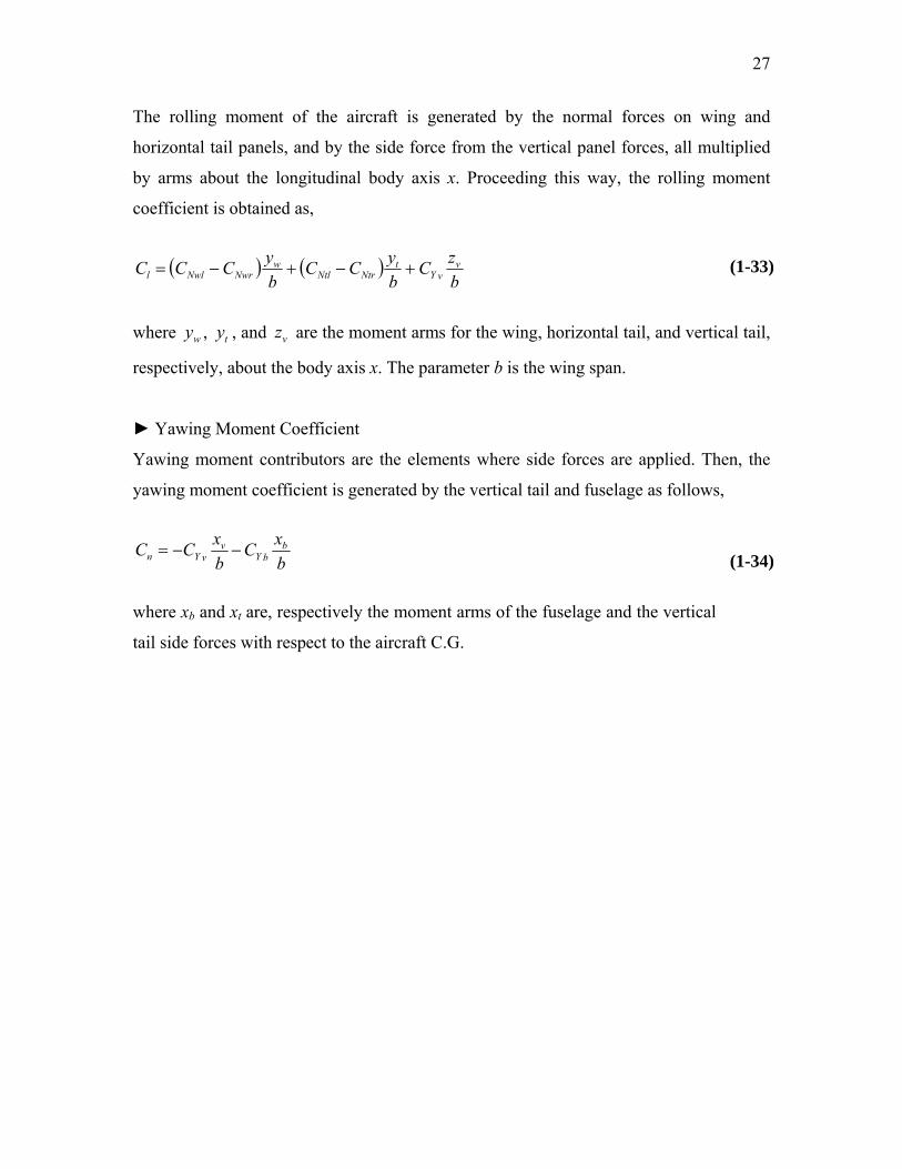
27
The rolling moment of the aircraft is generated by the normal forces on wing and
horizontal tail panels, and by the side force from the vertical panel forces, all multiplied
by arms about the longitudinal body axis x. Proceeding this way, the rolling moment
coefficient is obtained as,
( ) ( )bzC
byCC
byCCC v
vYt
NtrNtlw
NwrNwll +−+−=
(1-33)
where , , and are the moment arms for the wing, horizontal tail, and vertical tail,
respectively, about the body axis x. The parameter b is the wing span.
wy ty vz
► Yawing Moment Coefficient
Yawing moment contributors are the elements where side forces are applied. Then, the
yawing moment coefficient is generated by the vertical tail and fuselage as follows,
bxC
bxCC b
bYv
vYn −−= (1-34)
where xb and xt are, respectively the moment arms of the fuselage and the vertical
tail side forces with respect to the aircraft C.G.

28
1.2 The Wing Rock Phenomenon
Wing rock is defined in reference [41] as “uncommanded lateral-directional motion,
viewed by the pilot primarily as a roll oscillation.” For some types of aircraft
configurations, as the angle of attack further increases up to some critical value around 20
degrees a roll oscillation starts to grow in amplitude until it reaches a maximum value. At
this point, the airplane continues to rock in a classic limit cycle behavior. This behavior
occurs up to a higher critical value of the angle of attack (typically around 50 degrees).
After that higher critical value of the angle of attack value, the roll oscillations are
damped out.
This kind of phenomenon was first observed at NASA´s Langley Research Center around
1980 [42]. Wing rock can be described as a Dutch roll type of motion, during which the
aircraft has sustained rigid body oscillations predominantly in roll, but also in yaw. It can
appear in the subsonic flight regime and high angle of attack, or at transonic speeds and
more moderate values of angle of attack [43]. When any perturbation in roll happens at
higher values of the angle of attack, such as landing in crosswind or high load factor non-
coordinated maneuvers, wing rock can develop. A variety of aircraft exhibited this
phenomenon, but the most susceptible configurations have highly swept planforms or
strakes and long slender forebodies that produce vortical flows during excursions into the
high angle-of-attack regime. In general, it may adversely affect the whole flight envelope,
but it can be particularly dangerous if it happens during landing, when it limits the
approach angles of attack of military, commercial high-speed civil transport aircraft
configurations or orbital space shuttles. At higher speeds, it can also pose serious
limitation to combat effectiveness both in subsonic and in transonic flow regimes, and
severely limits the pilot’s ability to perform a tracking task.
Wing rock has been encountered during the development of many military aircraft in
service today. Some of the aircraft which have been documented to experience wing rock

29
are the A-4 Skyhawk, F-4 Phantom, F-5 Tiger, T-38 Talon, F-14 Tomcat, F-16 Fighting
Falcon, F-18 Hornet, X-29, X-31, HP-115 [44], Gnat trainer, Tornado, and Harrier.
We can see wing rock from two perspectives: from the global perspective of the flight
dynamics or the particular perspective of the physical mechanisms that happens on each
case. From the flight dynamics perspective, wing rock can be explained by the behavior
of the stability derivatives and the energy exchange concept [45], summarized in Section
(1.2.1) of this report. When it comes to the behavior of the stability derivatives, under a
certain critical value of the angle of attack, the airplane exhibits stable dynamic lateral
stability and roll motions following a disturbance damp out. This stable dynamic lateral
stability is equivalent to positive roll damping, which means negative . At a certain
angle of attack, roll damping becomes negative. As shown by Nguyen et al
plC
[45], a loss of
damping in roll at high angles of attack makes a configuration susceptible to wing rock
but does not necessarily generate a sustained wing rock. To generate a sustained wing
rock motion, an additional aerodynamic cause is necessary. For wing rock to occur, there
must be a nonlinear variation of roll damping such that negative damping (destabilizing)
exists at low values of sideslip/roll angle and positive damping (stabilizing) at higher
values of sideslip/roll angle.
The flow mechanism of the wing rock at high angles of attack depends on the aircraft
configuration, but the principal source of wing rock is the lifting surfaces. Thin, low-
aspect ratio, highly swept delta wings are prone to develop wing rock at high angles of
attack. However, aircraft configurations not having highly swept delta wings but
featuring fuselages with long, slender forebodies are also known to exhibit wing rock.
This latter type of wing rock is called wing-body wing rock or forebody-induced wing
rock and it is known to occur even when the main lifting surface - the wing - is removed.
For the configuration without the wing, the horizontal and vertical tail surfaces coming
under the influence of the forebody vortex system produce the necessary rolling
moments. From the published results on wing rock phenomenon, a good way to organize
ideas is to classify wing rock occurrences according to three main types: slender-wing
rock, conventional-wing rock, and wing-body rock, explained as follows.

30
Slender-wing rock is the occurrence of wing rock on highly swept-back, sharp leading
edge delta wings, alone or with blended bodies, at sufficiently high angle of attack. It is
triggered by some initial disturbance that initiates roll. Studies of the wing rock motion
on flat plate, slender delta wings have provided interesting insights on the importance of
unsteady aerodynamics to the wing rock motion [45], [46], [47]. At high angles of attack,
slender wing flow separates right at the leading edge and generates vortices (the leading
edge vortices). To describe the flow mechanism acting on this type of wing rock,
consider a delta wing with sweep angle equal or larger than 76 degrees at an angle of
attack between 20 and 50 degrees. Consider also a view from the trailing edge toward the
leading edge. Now, let us suppose that a disturbance causes the wing to initially roll in
the positive direction of the body axis. As the roll angle increases at a constant pitch
angle, angle of attack and sideslip are related to the roll angle through Eqs. (A.2-6) in
Appendix A.2. Because of these relations, the effective angle of attack on the wing
decreases and the effective sideslip angle increases as the roll angle grows. The increased
sideslip on the wing during roll causes the windward vortex on the down-going wing to
move inboard and toward the upper surface, and the leeward vortex to move outboard
and be lifted off. At a certain point, the rolling moment due to the vortex on the down-
going wing takes over the moment associated with the “lifted-off” vortex, and the
movement first stops and then reverts. When the roll angle is back to zero, the dynamic
hysteresis associated with the vertical location of the two leading edge vortices results in
a residual rolling moment that keeps the oscillations going on. It appears as if the vortices
have a sort of “inertia”: their vertical positions during oscillation have a delay when
compared to the static ones. We extracted from [46] figures 1-4 and 1-5 that show the
non-dimensional vertical and spanwise body coordinates of the vortices core, in addition
to the crossflow streamlines and pressure distribution curves, obtained from
computational simulations by using a discrete vortex potential model. It can be observed
that the lag in vortex position makes the upgoing wing closer to its corresponding vortex
core, and that these different positions results in the wing residual rolling moment at zero
roll angle.
31
Conventional wing rock is that occurring on airplanes having straight or moderate-swept
wings, and moderate to high aspect ratio. It can be subdivided into conventional-wing
rock that happens at low or at high subsonic Mach numbers. Because in this case the
wing aspect ratio is higher, two-dimensional streamwise flow effects dominate the
aerodynamics, and in the low subsonic regime this kind of wing rock is related to
dynamic stall [48]. According to tests made on the F-5A [43], at transonic speeds wing
rock was generated by a limit cycle mechanism due to the fluctuating pressure changes
on the wing top surface, especially near the wing tip region. In the cases observed, the
major reason for the pressure change was the motion-induced variations in local angle of
attack, which alternatively caused leading edge stall and recovery. Those fluctuating
pressure changes are caused by flow separation driven by the shock-boundary layer
interaction.
Forebody-induced wing rock is that type of wing rock that happens because of vortices
generated by the fuselage forebody. A generic aircraft model featuring a slender, pointed
fuselage forebody was used in tests described in [49]. This generic aircraft model
exhibited wing rock when fitted with different wings of varying aspect ratio and sweep,
or even without any wing at all. Therefore, for this type of wing rock, the wing itself was
not the primary cause of the motion. One possible explanation is the one found in
reference [50]. According to Ericson, at higher angles of attack, the airplane loses
damping in roll and sheds forebody vortices in an asymmetric way. These vortices are
convected towards the tail surfaces, sucked down over their upper surfaces and produced
the necessary rolling moments. Therefore, the lifting surfaces, either the wings or the tail
surfaces, when coming under the influence of forebody vortices, served as rolling
moment generators to sustain the wing rock. That is the reason that this kind of wing rock
is called forebody-induced wing rock.

32
Figure 1-7 Crossflow streamlines and pressure distribution (dot line) for zero roll
angle and positive roll rate. Figure reproduced from [46] with permission of the
author.

33
Figure 1-8 Crossflow streamlines and pressure distribution (dot line) for zero roll
angle and negative roll rate. Figure reproduced from [46] with permission of the
author.

34
1.2.1 The Energy Exchange Concept
When the model rolling moment coefficient as a function of the roll angle ( )φlC can be
determined for a wing undergoing wing rock, the energy exchange technique used by
Nguyen et al [45] is very helpful in analyzing the physical mechanisms driving the limit-
cycle oscillation. If we consider the case where the model is constrained to one degree of
freedom, the equation of motion for the system is
( ) ( )∑≈
+==876
&&0
frictionaeroRxx LLtLtI φ ( )tSbCq l∞=
(1-35) ( )
SbqI
tC xxl
∞
=⇒φ&&
Thus, when the model geometry, inertia, wind tunnel test conditions and roll angle time
history are known, the rolling moment coefficient time-history ( )tCl can be determined.
The energy added to or extracted from the system during the motion for a specific time
interval can be expressed as
( )∫∞=Δ2
1
t
tl dttCbSqE φ& (1-36)
Eq. (1-36) may be rewritten in terms of the instantaneous roll angle ( )tφ as the following
line integral:
( )[ ]∫∞=Δφ
φφC
l dtCbSqE (1-37)
where is the curve obtained by plotting as a function of the instantaneous roll
angle
φC lC
( )tφ for the interval [ . Therefore, the energy exchanged in a cycle of motion is
directly related to the area enclosed by .
]21,tt
φC Figure 1-9 shows the conceptual drawings of

35
possible cases for , where the arrows indicate the direction in time. When the loop
encloses an area in a clockwise sense, energy is being added to the system (
φC
Figure 1-9a),
whereas counterclockwise loops indicate energy dissipation from the system (Figure
1-9b). If a limit cycle occurs, the net energy exchange is zero (Figure 1-9c). Figure 1-10
shows the actual roll angle time-history of a slender delta wing at an angle of attack
where the roll oscillations damp out. It was obtained from wind tunnel tests by Arena,
and reported in [46] and [51]. The corresponding φ×lC loop is shown in Figure 1-11.
Figure 1-12 presents a time history of wing rock buildup at °= 300θ for tests reported in
[51]. The dynamic rolling moment characteristics of the buildup cycle A are shown in
Figure 1-13, where the clockwise loop in the plot indicates a dynamic instability. Notice
that the restoring moment is roughly linear with roll angle. Since energy is being fed to
the system, the roll angle amplitude is increasing. When the loop is very thin like the one
shown, it accounts for the fact that the buildup happens very slowly. The analogous plot
of the rolling moment coefficient after the system has reached steady state (cycle B) can
be seen on Figure 1-14. There still is an unstable region between -20° and 20°, but two
stable damping “lobes” have formed for the larger roll angles. The limit cycle oscillation
is sustained because the area of the lobes equals the area of the unstable portion of the
plot such that the net energy exchange is zero.

36
Figure 1-9 Conceptual drawings of the rolling moment coefficient versus roll angle.
Figure reprinted from [52] by permission of the author.

37
Figure 1-10 Roll angle time-history for wing pitch angle where there is no wing
rock. Figure reprinted from [46] by permission of the author.
Figure 1-11 Rolling moment coefficient vs. roll angle cycle for a wing pitch angle
where there is no wing rock. Figure reprinted from [46] by permission of the author.

38
Figure 1-12 Time history of wing rock buildup in free to roll tests at wing pitch
angle equal 30 deg. Figure reproduced from [46] by permission of the author.
Figure 1-13 Rolling moment coefficient for a cycle of wing rock buildup. Figure
reproduced from [46] by permission of the author.

39
Figure 1-14 Rolling moment coefficient for a steady state cycle of wing rock. Figure
reprinted from [46] by permission of the author.
1.2.2 Experimental Investigations on the Slender Delta Wings
This is a brief review of the references where unsteady aerodynamic measurements and
wing rock motion data were taken and used to identify unsteady aerodynamic models
investigated along the same lines as this research. As previously mentioned, the principal
source of wing rock is the lifting surfaces. Furthermore, some of the aircraft unsteady
aerodynamic models investigated here are a composition of basic aerodynamic models
that represent the unsteady aerodynamic behavior of each of the lifting surfaces. Since
these models include internal state variables that describe the flow characteristics, their
construction is heavily based on observations made on the available experimental data.
Most of the published experimental data is for slender delta wings. Also, because the
most susceptible configurations to wing rock have highly swept planforms or strakes that
produce vortical flows during excursions into the high angle-of-attack regime, it is

40
thought that the mechanisms which are present in the wing rock of slender delta wings
will also be the dominant effects in the wing rock of complete aircraft configurations.
Thus we focus our attention on this kind of lifting surface.
The experimental work done by Nguyen, Yip, and Chambers [45] at NASA Langley
provides data that helps us understand the fundamental flow mechanisms causing wing
rock for slender delta wing configurations. This experimental work also led to the Energy
Exchange Concept, described in Section 1.2.1, which is important to the current work.
The data published in that reference for the slender delta wing free-to-roll dynamic tests
are used here to identify the model parameters of the investigated formulations. As
discussed in Section 1.2.1, analysis of the motions obtained in the free-to-roll tests were
made by the analysis of the measured roll angle data. Nguyen et al. were able to derive an
estimate of the roll acceleration by fitting a smoothing cubic spline to the roll angle time
history data points, thus eliminating high frequency noise. With the roll acceleration
determined, an estimate of the total aerodynamic rolling-moment coefficient was derived
through Eq. (1-35). With the roll angle and the total aerodynamic time-histories, Nguyen
et al were able to plot the φ×lC loops for the angles of attack equal to 27 and 32
degrees, as shown in Figures 1-15 and 1-16 and used in this research to identify
parameters associated with the dynamic behavior.
Levin and Katz [47] have also conducted free to roll tests on 76 and 80 degree swept
delta wings. Only the delta wing with a sweep angle equal to 80 degrees and an aspect
ratio of 0.71 (root chord = 0.4285 m, span = 0.150 m) demonstrated wing rock in the free
to roll tests documented in that reference. In their experiments, static force and moment
data were obtained. The corresponding experimental results for the static tests, shown in
Figure 1-17 and Figure 1-18 for roll angles of 0, 10, 20 and 30 degrees, and for an
airspeed of 14 m/s, helped to identify the unsteady aerodynamic model parameters
associated with the static behavior of the model investigated in this research. Concerning
the dynamic data, Levin and Katz obtained time histories of the roll angle, and of the
lateral and normal force coefficients. However, they were not able to acquire
experimental values for the rolling moment coefficients.

41
Figure 1-15 Cl vs. roll angle histogram for one cycle of wing rock at θ0 = 27 degree .
Data extracted from [45].
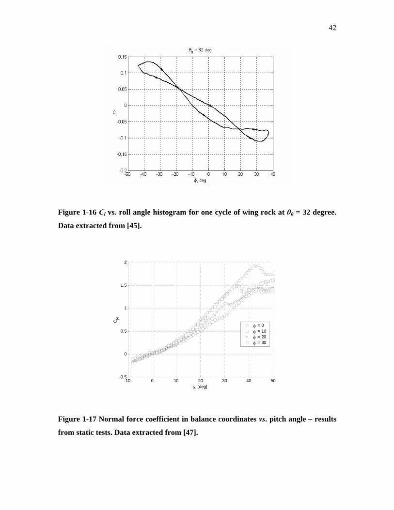
42
Figure 1-16 Cl vs. roll angle histogram for one cycle of wing rock at θ0 = 32 degree.
Data extracted from [45].
-10 0 10 20 30 40 50-0.5
0
0.5
1
1.5
2
α [deg]
CN
φ = 0φ = 10φ = 20φ = 30
Figure 1-17 Normal force coefficient in balance coordinates vs. pitch angle – results
from static tests. Data extracted from [47].

43
-10 0 10 20 30 40 50-0.1
-0.08
-0.06
-0.04
-0.02
0
0.02
α [deg]
Cl
φ = 0φ = 10φ = 20φ = 30
Figure 1-18 Rolling moment vs. pitch angle – results from static tests. Data
extracted from [47].
Another reference that contains experimental data useful in the identification of the basic
unsteady aerodynamic models investigated here is the one written by Arena [46]. The
primary goal of that experimental investigation was to document motion history and flow
field behavior on a slender delta wing undergoing wing rock to identify mechanisms that
may be responsible for wing rock. Two delta wing models with a leading edge sweep
angle of 80 degree were used. One of them was used for flow visualization and free-to-
roll time histories determination. The other was instrumented for the steady and unsteady
measurement of surface pressure. The main features of the experimental apparatus were
the air bearings and the modular optical encoder, installed with the purpose of having a
single degree of freedom motion with little friction from the bearing or from roll angle
acquisition. The work documented the angle of attack range where wing rock exists for
this particular wing, at a Reynolds number of 400,000. Inside that range, initial angles of
attack were chosen to represent damped motion ( °= 20α ) and limit cycle wing rock
( °= 30α ). The corresponding rolling moment coefficient vs. roll angle loops are

44
reproduced here in Figure 1-11 and Figure 1-14, respectively. The measurement of the
rolling moment acting on the wing was possible by finite differencing the motion history
of the wing. In order to have further insight into how the surface pressure creates the
rolling moment, a motion control system was developed to guide the model through the
wing rock time histories obtained in the free to roll experiments. The steady and unsteady
flow visualization of vortex trajectories allowed measurements of the vortex core location
for the wing undergoing wing rock, reproduced in Figure 1-19 for the chord location of
75%, providing the vortex positions above a slender delta wing as a function of the roll
angle during wing rock motion, and helped to shape the internal state equations of some
of the unsteady aerodynamic models proposed and investigated here. The coordinate
system used to give the positions of the vortex cores is shown in Figure 1-20. It was
found that vortex breakdown is not a primary mechanism involved in the slender-wing
rock motion, since it is not seen on the wing over a large range of angles of attack at
which wing rock occurs. But when it occurs over the model, additional damping is added
which results both in an overall reduction in the wing rock amplitude and in a jump in the
reduced frequency. However the author stated that it is just an additional contribution to
the damping and not one of the primary mechanisms responsible for the occurrence of the
wing rock.
The geometrical and physical differences between the wing models and experimental
apparatus used in the tests published in [45], [46], and [47] are summarized in Table 1-1.
The wings were fixed to the sting in different ways. The free to roll apparatus used by
Nguyen, Yip, and Chambers [45] had its bearings and the potentiometer used to measure
the roll angle located beneath the wing. This caused the center of rotation of the model to
be two inches below the longitudinal axis of the wing. A sketch of this apparatus is
shown on Figure 1-21. Levin and Katz managed to mount the bearings and potentiometer
on the wing centerline. This caused the wing to have a relatively large center body hump,
as shown in Figure 1-22.

45
1.2.3 Analytical and Computational Investigations on the Wing Rock
Konstadinopoulos, Mook, and Nayfeh [53] numerically reproduced the slender delta
wing wind tunnel tests whose results were published in [45], [47]. They used an unsteady
vortex-lattice method (UVLM) to provide the aerodynamic loads and integrated the
single degree-of-freedom equation of motion using a predictor-corrector scheme. The
UVLM was coupled with the equation of motion and both the motion and the flow field
were predicted interactively. Their simulations considered the geometrical and physical
differences between the experimental apparatus used in both tests, as well as the damping
due to the friction in the bearings of the stings. Simulations were done for the case where
the axis of rotation was below the centerline of the wing, reproducing the arrangement
used by Nguyen et al [45] in their tests, and also for the case where the axis of rotation
was on the centerline, as in the experiments reported in [47]. An analytical representation
of the rolling moment was developed to help the understanding of the wing rock
dynamics. In this representation, the rolling moment is represented by the expansion in
terms of angle of roll φ and roll rate given by Eq. φ& (1-38).
( ) 57
36
25
24
3321, φφφφφφφφφφφ aaaaaaaCl ++++++= &&&&&
(1-38)
5432324 &&&&&12111098 φφφφφφφφφ aaaaa +++++
In Eq. (1-38), the coefficients were determined by a least-squares fit with the
numerical results found with the help of the UVLM. Since the curves of the rolling
moment coefficient vs. angle of roll
ia
lC φ change with the angle of attack, so do their
coefficients. It was observed that some of the terms in Eq. (1-38) make virtually no
contribution and their coefficients can be set equal to zero. This is the case for the
coefficients . The simulations showed that when the angle of attack
exceeds a critical value, the limit cycle develops after a small perturbation in roll. The
UVLM is limited to angles of attack for which vortex bursting does not occur and to
situations in which separation occurs only along the edges.
12111098 ,,,, aaaaa

46
Later, the nonlinear analysis of Eq. (1-38) was carried out in [54]. The analytical result
was used to construct phase planes by using the method of multiple scales, and the global
nature of the wing rock was revealed through stable limit cycles, unstable foci, saddle
points, and domains of initial conditions that lead either to sustained oscillatory motion,
divergence or damping.
In addition to his experimental work, summarized here in Section 1.2.2, Arena [46]
investigated the steady and unsteady behavior of delta wings in roll also with the
development of a computational model since there were certain aspects of the flow field
that could not be revealed with the experimental apparatus. For example, it was not
possible to measure the unsteady behavior of vortex strength during wing rock. His
computational model represented the separated flow field above the wing as a system of
two discrete vortices in an inviscid flow. The position and strength of each vortex was
captured by the formulation of specific boundary conditions. The idea was to use this
computational model to capture the primary mechanisms responsible for wing rock that
had not been captured during the wind tunnel tests, such as the vortex strength influence.
According to Arena’s conclusions in [46], vortex strength hysteresis on the downward
wing contributes with a rolling moment that opposes the direction of rotation and helps to
stabilize the wing at the higher values of the roll angle.
Saad [55] numerically simulated three degree of freedom wing rock motion through the
flow solver code fdl3di: roll, sideslip and vertical motion. The results were obtained for a
generic fighter model consisting of fore-body, cropped delta wing and vertical fin. Until
then, wing rock numerical simulations had been limited to a single degree of freedom in
roll and applied to simple delta-wing configurations. He studied the additional effects of
sideslip and vertical motion, as well the effect of adding the vertical fin. The effect of
adding the sideslip and vertical motion degrees of freedom to the simulations of the wing-
body configuration were found to delay the onset and to reduce the amplitude of wing
rock by about 50% with no change in frequency. The aerodynamic effect of the fin was
found to delay the vortex burst on the upper surface of the wing. As a net result of the
47
vertical fin inclusion, the oscillations were more damped, with significant increase in
frequency.
1.3 Overview of the Thesis
The goal of the current research is to investigate functional, unsteady aerodynamic
models with a state-space representation that could be coupled to the equations of motion
to simulate wing rock. To achieve these goals, we insert modifications into an existing
basic unsteady aerodynamic formulation and identify its parameters using published
experimental data for slender delta wings. Since the identification results obtained with
the pre-existing formulation are not satisfactory, we first develop a basic unsteady
aerodynamic model that is capable of accounting for the static hysteresis phenomenon.
Then, we add additional internal state variables representing both the spanwise and
vertical motion of the vortex core, which account for the sideslip and roll angle on the
lifting surface normal force. Next, we apply this model to each one of the lifting surfaces
or panels in which the aircraft is split, and investigate its ability to represent the wing
rock phenomenon. The unsteady aerodynamic model is finally coupled to the equations
of motion to perform simulations of the wing rock phenomenon.
The proposed models are described in Ch. 2. The identifications of their model
parameters are shown in Ch. 3. Chapter 4 presents the simulations done with the models
that were identified. Some final comments and conclusions are presented in Chapter 5.

48
Figure 1-19 Vertical and spanwise vortex positions during wing rock. Data extracted
from [46]. (a) Vertical position. (b) Spanwise position.

49
Table 1-1 Geometrical and physical parameters of some tested slender delta wings.
Wing 1 Wing 2 Wing 3
[45] [47] [46]
root chord cr, m 1.765 0.4285 0.422
planform area S, m2 0.5491 0.0321 0.0314
span b, m 0.622 0.150 0.149
rolling moment of inertia , xxI
kg m2
9.18 210−× 2.7 410−× 1.13 310−×
ρ , kg/m3 1.187 1.2 1.2
∞V , m/s 9.266 15 13.8
Figure 1-20 Sketch of asymmetric vortex position – rear view. Figure reprinted
from [46] by permission of the author.

50
Figure 1-21 Free to roll apparatus used by Nguyen, Yip, and Chambers. Figure
reprinted from [45] by permission of the American Institute of Aeronautics and
Astronautics, Inc.

51
Figure 1-22 Free to roll apparatus used by Levin and Katz [47]. Figure
reprinted by permission of the American Institute of Aeronautics and
Astronautics, Inc.

52
2 The Investigated Unsteady Aerodynamic Models
Unsteady aerodynamic effects at high angles of attack resulting from separated and
vortex flow development can significantly alter the aerodynamic loads with respect to
their conventional representation. In the conventional approach, the unsteady effects are
described using linear terms with unsteady aerodynamic derivatives. Nevertheless, there
are special regions of incidence, e.g. , where the conventional representation is not
valid. Since in unsteady flight conditions the aerodynamic forces and moments are time
and motion history dependent, a dynamic model is needed for the development of a valid
description. The special approaches using the differential equations that have been
proposed can improve the aerodynamic model and take into account the nonlinear
unsteady aerodynamic effects due to separated and vortex flow dynamics. A basic state-
space model with state-space representation was studied in refs.
maxLC
[30], [32], [34], after the
ideas of Goman and Khrabrov proposed in [29]. This general concept was described in
Section 1.1.3. Fan and Lutze proposed in [30], [34] a variation of this model, and some of
their contributions are mentioned in Section 1.1.3, as well. As a difference to the Goman
and Khrabrov version, the variation proposed by Fan and Lutze uses the distance between
the wing trailing edge and the separation point as the internal state variable, instead of the
distance between wing leading edge and the separation point used by the Russian authors.
The reason behind this choice was to have aerodynamic coefficients at low angles of
attack independent of the internal state variable. That made this model more consistent
with the conventional approach. De Oliveira and Lutze [32] added to this formulation an
improvement that allows it to represent static hysteresis. The description of this
improvement was described in Section 1.1.5.
The application of the exact original state-space model to the rolling delta wing has some
problems. One of them is that the separation point has different values for each of the
side of the wing, and consequently so does the internal state variable. Another problem is
that the angles of attack are different for each side of the wing when the wing is rolling.

53
Both of these problems make it difficult to use only one output equation to determine
each aerodynamic coefficient. In a tentative approach to address the unsteady
aerodynamic characteristics in multiple axes, Stagg and Lutze [39],[40] proposed
dividing the airplane lifting surfaces into separate panels, and applied the basic state-
space model to characterize the unsteady aerodynamics of each one of them in the way
described on Section 1.1.6. Here this panel formulation describing the unsteady
aerodynamic characteristics of the aircraft in multiple axes is composed with some
proposed basic unsteady aerodynamic models and investigated. The investigation starts
with a model whose improvements over the original Stagg and Lutze model allows it to
match some influences of the roll (or the sideslip) angle. Also, the basic unsteady
aerodynamic model used in each panel is that described in Section 1.1.5, which is
improved to represent static hysteresis. The second model investigated has some further
modifications, for example, the addition of both the roll angle as an input variable, and of
two internal state variables.
Since the acquisition of wind tunnel experimental data was not part of this research, all
the investigated models have their parameters identified with data available for slender
delta wings taken from published references. The slender delta wing geometries and the
data used to identify the model parameters are described in Section 3.2.
2.1 The First Unsteady Aerodynamic Model Investigated
The original state-space model was found to have good performance in describing the
unsteady aerodynamics of the airplane when considered as a single lifting surface up to
high angles of attack [29], [30], [34]. Nevertheless, this good performance was observed
only for longitudinal motion, in which the only motion variable was the angle of attack.
Trying to take advantage of the state-space formulation to find the simplest model that
could describe the unsteady aerodynamics of the whole airplane in multiple axis, Stagg
and Lutze [39],[40] proposed dividing the airplane into panels that represent lifting
surfaces, and applied the basic state-space model presented in [30], [34] to characterize
the unsteady aerodynamics of each one of them in the way described in Section 1.1.6.
When the rolling moment coefficient was plotted against the sideslip angle in [39] for the

54
F-18 forced to oscillate in roll at pitch angle equal to 30 degrees with amplitude of 20
degrees and a frequency of 1 Hz, the result is shown in Figure 2-1, where the arrows
indicate direction in time. Comparing it to Figure 1-9, we can see that, according to the
Energy Exchange Concept [45] described in Section 1.2.1, this model would not undergo
limit cycle oscillations if the F-18 model was left free to rotate. Another try was made
here to verify if a model based on this formulation could simulate wing rock by adding
some improvements and identifying its parameters with the help of simulated
experimental data.
-15 -10 -5 0 5 10 15-0.04
-0.03
-0.02
-0.01
0
0.01
0.02
0.03
0.04
Cl
β, degree
Figure 2-1 Roll coeficient versus sideslip angle for the F-18
Considering Figure 1-17, we notice that there is a different CN vs. α curve for each value
of the roll angle, and they have not only different slopes but also different angles of stall.
One of the reasons for the different slopes is because the wing normal coefficient CN
values shown in Figure 1-17 are represented in balance coordinates. That means that,
because the wind tunnel balance used to take the experimental values of the delta wing
normal coefficient recorded only the vertical component, then to be compared to the NC

55
experimental results the values of the wing normal coefficient in body axes have to
be converted to the normal coefficient in balance coordinates
NC
( )balNC through Eq. (2-1)
below:
( ) φcosNbalN CC = (2-1)
where φ is the roll angle and is the wing total normal coefficient in body axes. NC
Another possible reason for the slopes of the CN vs. α curve being different for each
value of the roll angle could be the wing aerodynamic characteristics variation with the
sideslip angle.
When the multi-axis state-space representation (see Section 1.1.6) is applied to the
slender delta wing configuration, it is split into two lifting panels: left and right semi-
wings, so we drop the subscript “w”. Since this type of configuration has not tails, the
number of parameters to be identified is less than the one corresponding to a conventional
aircraft. In the present case, we have four unknowns: the left and right normal force
coefficients and moment arms. Also reduced in number are the equations used: in the
static case we have just one normal force equation like the first term of (1-30), and the
rolling moment equation (1-33). There still is the dynamic relationship that we assumed
between the normal forces on left and right wings (1-18), and the number of unknowns is
reduced to three.
Comparing Eq. (1-33) with Figure 1-18 one can notice that, when applied to that wing-
alone configuration, the original Stagg formulation does not have flexibility to account
for the variation of the rolling moment coefficient static values with the angle of attack
and with the roll angle variations. This happens because, in the multi-axis original
formulation, the lateral arm yw has the same value for left and right wings. Also, in the
static case, the normal force coefficient static values on both wings are the same because
the angles of attack on both left and right wings have the same values. Consequently, if it
was calculated through that formulation, the static responses of the rolling moment
coefficient would be zero for all values of the roll angle and the original model will never

56
match the experimental data. To add more flexibility to Stagg’s formulation, we define,
as additional model parameters, the set containing one different parameter for each of the
left and right wing lateral arms ywl, ywr , free to vary with the roll angle (see Table 3-1).
The results of the identification done for this first improvement to the Stagg’s
formulation only using static experimental values, and are shown on Figure 2-2 and
Figure 2-3. This parameter identification was done by a least –squares fit between the
calculated values of the normal force and rolling moment coefficients and the
experimental data taken from reference [47]. More details about the parameter
identification can be seen in Chapter 3. Figure 2-4 shows the variation of the identified
wing lateral arms with the roll angle. We see in Figure 2-2 and Figure 2-3 that the
experimental values of the angle of stall change with the roll angle. The original
formulation does not have the flexibility to account for that either. Trying to improve still
further the match between the model responses and the experimental data, we let the
parameters and ∗α σ vary with the roll angle such that there is one different identified
value of each parameter per roll angle value (see Table 3-1). Finally, the series expansion
of in NC α and α& in Eq. (1-18) is also increased to a higher order in Eq. (2-5), due to
the high nonlinearity exhibited by the experimental data. After adding these
modifications, the first unsteady aerodynamic model for the slender delta wing to be
investigated is obtained and summarized through Eqs. 2-2 to 2-7. The notation used is
similar to that of Section 1.1.6.

57
► State equations:
( )iiii
x xxdtxd
ατατ α &,20,1 −=+ (2-2)
► Output equations:
(2-3) rNlNN CCC ,, +=
rrNllNr
rNl
lNl yCyCby
Cby
CC −=−= , (2-4)
where
( ) ( ) ( ) ( ) ( ) iiiNiiNiiNiiNiiNNiN xCxCxCxCxCCC αααααααααααα
ˆˆˆˆ
2ˆˆ
20 22 &&&
&&&+++++=
(2-5)
with i = l (left), r (right) panel, and . t̂ ˆ αα && =
The spanwise positions ly , ry of the normal force point of application, the sigmoid
location angle of attack and the slope ∗α σ are made functions of the roll angle. The
remaining functions and parameters for this formulation are:
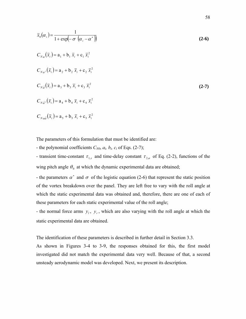
58
( ) ( )( )∗−−+=
αασα
iix
exp11
0 (2-6)
( ) 2111 c ba iiiN xxxC ++=α
( ) 2222 c ba2 iiiN xxxC ++=α
( ) 2333ˆ c ba iiiN xxxC ++=α& (2-7)
( ) 2444ˆ c ba2 iiiN xxxC ++=α&
( ) 2555ˆ c ba iiiN xxxC ++=αα &
The parameters of this formulation that must be identified are:
- the polynomial coefficients CN0, ai, bi, ci of Eqs. (2-7);
- transient time-constant x,1τ and time-delay constant ατ ,2 of Eq. (2-2), functions of the
wing pitch angle 0θ at which the dynamic experimental data are obtained;
- the parameters and ∗α σ of the logistic equation (2-6) that represent the static position
of the vortex breakdown over the panel. They are left free to vary with the roll angle at
which the static experimental data was obtained and, therefore, there are one of each of
these parameters for each static experimental value of the roll angle;
- the normal force arms , , which are also varying with the roll angle at which the
static experimental data are obtained.
ly ry
The identification of these parameters is described in further detail in Section 3.3.
As shown in Figures 3-4 to 3-9, the responses obtained for this, the first model
investigated did not match the experimental data very well. Because of that, a second
unsteady aerodynamic model was developed. Next, we present its description.
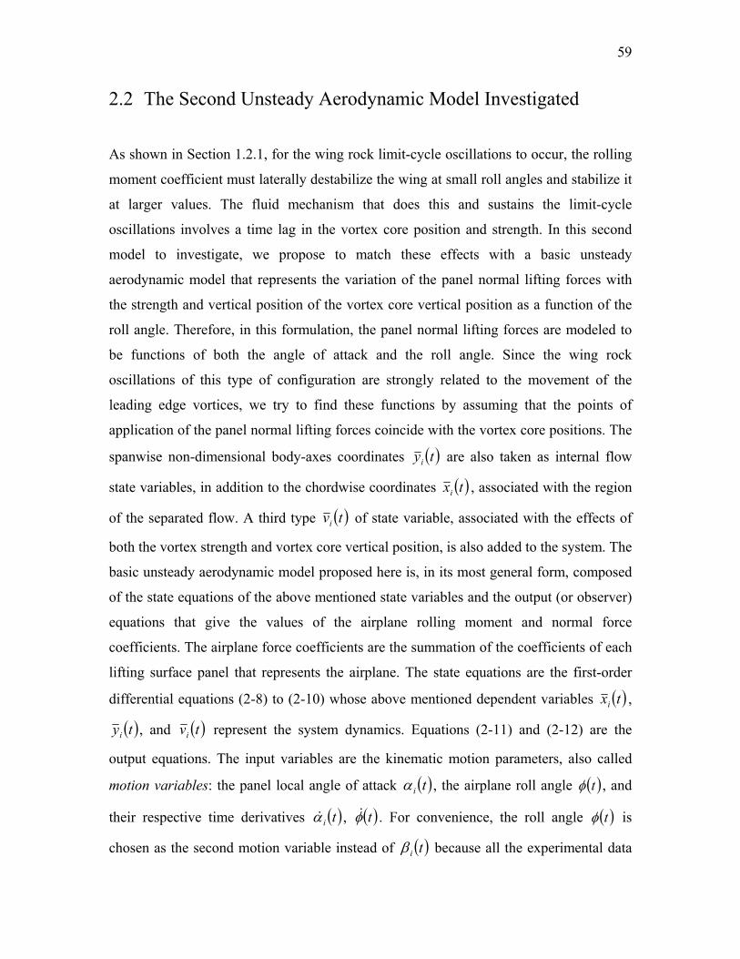
59
2.2 The Second Unsteady Aerodynamic Model Investigated
As shown in Section 1.2.1, for the wing rock limit-cycle oscillations to occur, the rolling
moment coefficient must laterally destabilize the wing at small roll angles and stabilize it
at larger values. The fluid mechanism that does this and sustains the limit-cycle
oscillations involves a time lag in the vortex core position and strength. In this second
model to investigate, we propose to match these effects with a basic unsteady
aerodynamic model that represents the variation of the panel normal lifting forces with
the strength and vertical position of the vortex core vertical position as a function of the
roll angle. Therefore, in this formulation, the panel normal lifting forces are modeled to
be functions of both the angle of attack and the roll angle. Since the wing rock
oscillations of this type of configuration are strongly related to the movement of the
leading edge vortices, we try to find these functions by assuming that the points of
application of the panel normal lifting forces coincide with the vortex core positions. The
spanwise non-dimensional body-axes coordinates ( )tyi are also taken as internal flow
state variables, in addition to the chordwise coordinates ( )txi , associated with the region
of the separated flow. A third type ( )tvi of state variable, associated with the effects of
both the vortex strength and vortex core vertical position, is also added to the system. The
basic unsteady aerodynamic model proposed here is, in its most general form, composed
of the state equations of the above mentioned state variables and the output (or observer)
equations that give the values of the airplane rolling moment and normal force
coefficients. The airplane force coefficients are the summation of the coefficients of each
lifting surface panel that represents the airplane. The state equations are the first-order
differential equations (2-8) to (2-10) whose above mentioned dependent variables ( )txi ,
( )tyi , and ( )tvi represent the system dynamics. Equations (2-11) and (2-12) are the
output equations. The input variables are the kinematic motion parameters, also called
motion variables: the panel local angle of attack ( )tiα , the airplane roll angle ( )tφ , and
their respective time derivatives ( )tiα& , ( )tφ& . For convenience, the roll angle ( )tφ is
chosen as the second motion variable instead of ( )tiβ because all the experimental data

60
used to find the model parameters were published as a function of ( )tφ . For each fixed
value of the wing pitch angle 0θ , the local sideslip angle time history ( )tiβ can be
determined through ( )tφ and ( )tiα time-histories by using Eqs. (1-22) and (1-28),
derived in Appendix A.2. However, for a general type of motion where the pitch angle is
not fixed, those relations are no longer valid.
In this postulated model, the equations used to represent the unsteady aerodynamics for
general flight conditions in each panel of the airplane are:
( ) ( )iiii f
dttxd
αα &,,1= (2-8)
( ) ( )φφ &,,2 ii f
dt=
tyd (2-9)
( ) ( )φφ &,,3 ii f
dttvd= (2-10)
( )φφαα && ,,,,,, iiiiiN yxgC = (2-11)
where the subscript i stands for each lifting panel, i.e., i = l (left) , r (right).
The value of the normal force coefficient for the whole slender delta wing is found also
through Eq. (2-3).
As shown in Section 1.1.6, we can calculate the rolling moment coefficient for the
aircraft through Eq. (1-33), which in the particular case of the slender delta wing reduces
to:
( ) ( )φφ rrNllNl yCyCC −= (2-12)
where ( )•y are the non-dimensional arms of the normal force coefficient with respect to
the longitudinal body axis, given by Eq. (2-9).

61
With the help of the formulation described in Section 1.1.5, the system composed by the
Eqs. (2-8), (2-9), (2-10), and (2-11) results in the following equations:
( ) ( )ieffDieffUii
x xDxUxdtxd
,,0,,01 αατ αα +=+ (2-13)
( ) ( )effDieffUiii
y yDyUydt
φφτ φφ ,,0,,01 +=+yd
(2-14)
( ) ( )effDieffUiii
v vDvUvdtvd
φφτ φφ ,,0,,01 +=+ (2-15)
( ) ( )φα ,, ,,, iiNiiiNiN vCxCC Δ+= (2-16)
We do this because we want this model to be capable of representing static hysteresis,
whenever it occurs. Equation (2-13) is the same as Eq. (1-12), that is,
( )2
1 αα
Δ+=Δ signU
(2-17)
( )2
1 αα =D Δ−Δ sign
(2-18)
with jj ααα −=Δ +1 for the given sequence of the static angles of attack jα , j = 1,2,…,l,
or ( ) ( )jj tt ααα −=Δ +1 for the given time histories of angles of attack ( ){ }njj ttt ≤≤0,α
in the considered panel. The static dependence between the internal state variable ix and
the angle of attack are determined for the up (U) and down (D) direction by
( )[ ]∗−−+=
UieffUxUx
αασ ,,0 exp1
1
(2-19)
( )[ ]∗−−+=
DieffDxDx
αασ ,,0 exp1
1 (2-20)

62
Since all the effects due to the sideslip or to the roll angle are now included in the term
( )φiNC ,Δ of Eq. (2-16), the parameters and ∗•)(α )(, •xσ related to the localization and
shape of the sigmoids given by Eqs. (2-19) and (2-20) are not let free to vary with the roll
angle in this case. The values of effα are determined through the equation
(2-21) iiieff αταα α &,2, −=
with ατ ,2 being a time-delay constant related to the vortex burst location. Equation (2-14)
is similar in structure to (2-13), and its nomenclature is given as follows,
y1τ = the transient time-constant related to the vortices core spanwise displacement.
by
y ii = = non-dimensional distance between the panel normal lifting force point of
application and the longitudinal axis.
( )2
1 φφ
Δ+=Δ signU
(2-22)
( )2
1 φφ =D Δ−Δ sign
(2-23)
with jj φφφ −=Δ +1 or ( ) ( )jj tt φφφ −=Δ +1 respectively in the quasi-static and in the
dynamic cases, where, in the quasi-static case, the given sequence of the static roll angles
is jφ , j = 1,2,…,l, and where ( ) ( )ii tt φφφ −=Δ +1 for the given time histories of roll angles
( ){ nii ttt ≤≤0, }φ . The time-delay effects on the vortex movements due to the roll angle
are taken into account through
φτφφ φ&
,2−=eff , (2-24)
where φτ ,2 is a time-delay constant related to the vortex core position, to be found from
wind tunnel data.
Since the vortex strength and vertical core position effects are considered to be lumped
into Eq. (2-15), we want the state variables iy to behave qualitatively like the wind

63
tunnel tests results shown in Figure 1-19. That means that iy must get smaller for the
panel that is going down. Because of that, the logistic functions that compose the right-
hand-side of (2-14) are built as follows,
( ) ( )[ ]∗−+=
UiyUiyiUiy
,,,,,,0 exp1
1φφσξ
φ (2-25)
( ) ( )[ ]∗−+=
DiyDiyiDiy
,,,,,,0 exp1 φφσξφ 1
(2-26)
where 1−=lξ and 1=rξ respectively for left (i = l) and right (i = r) panels. Symbols
( )•,,iyσ and stand respectively for the slope and roll angle location of the logistic
functions that represent the static variation of the vortex spanwise position with the roll
angle.
( )∗
•,,iyφ
The state variable v is defined to represent the increase in panel lift due to both the
increase in vortex strength and the approximation of the vortex core to the panel upper
surface, as the wing rolls. Because of that, the forcing terms of on the right-hand side of
Eq. (2-15) are modeled to be
( ) ( )[ ]∗−−+=
UivUiviUiv
,,,,,,0 exp1
1φφσξ
φ (2-27)
( ) ( )[ ]∗−−+=
DivDiviDiv
,,,,,,0 exp1 φφσξφ 1
(2-28)
In these last equations, the symbols ( )•,,ivσ and stand respectively for the slope and
roll angle location of the logistic functions that represent the static variation of the effects
of vortex vertical position and strength with the roll angle.
( )∗
•,,ivφ
In Eq. (2-16), the first parcel ( )iiN xC α,, is taken as it was developed in [34], that is, as
the following expansion in terms of the angle of attack α and its non-dimensional time-
derivative , for the roll angle equal zero: α̂&

64
(2-29) ( ) ( ) ( ) ( ) iiiNiNiiNiiNiiNNiN xCCxCxCxCCC αααααα αααααα
ˆˆˆˆ
2ˆˆ
20, 22 &&&
&&&+++++=
where
(2-30)2)( ijijjiN xcxbaxC ++=χ
with , and ααααααχ ˆ,ˆ,ˆ,, 22 &&&= 5,4,3,2,1=j , respectively. The motion variable is
the non-dimensional angle of attack rate and t is the characteristic time of the flow
defined as in Eq.
αα && t̂ˆ =
ˆ
(1-17).
In Eq. (2-16), ( )φiNC ,Δ is the parcel that accounts for the effects of the roll angle at a
fixed pitch angle value 0θ . It is this normal force term that accounts for the effects due to
both vortex vertical position and strength. The normal lifting force on a panel gets bigger
as the roll angle changes in a way that makes the panel go down. Also, it was shown in
[46] that the limit-cycle oscillations are sustained by a time lag in vortex core position
and strength. To make this model capable of handling these variations in a nonlinear way,
the panel normal force ( )φiNC ,Δ is built according to the following dependence of the
roll angle φ and of the non-dimensional roll rate : φ̂&
( ) ( ) ( ) ( ) 53, 53, φφφφ φφφ iNiNiNiiN vCvCvCvC ++=Δ ( ) ( ) 3ˆˆ
3 φφ φφ&&
&& iNiN vCvC ++
( ) ( ) 2222 φφφφ φφφφ
&&&& iNiN vCvC ++ ˆˆ
(2-31) where
Vb
2ˆ φφ && = (2-32)

65
( ) 2666 iiiN cbaC νννφ ++=
2777)(3 iiiN vcvbavC ++=φ
2888)(5 iiiN vcvbavC ++=φ
2999)( iiiN vcvbavC ++=φ&
(2-33)
2101010)(3 iiiN vcvbavC ++=φ&
2111111)(2 iiiN vcvbavC ++=φφ &
2121212)(2 iiiN vcvbavC ++=φφ &
V = free stream airspeed.
The coefficients , are functions of the angle of attack, and are determined by a
least-squares fit with the experimental data. The expansion terms in Eq.
jjj cba ,,
(2-31) were
picked in order to match the expansion developed by Konstadinopoulos, Mook, and
Nayfeh for ( )φlC in [53].
The parameters to be identified using wind tunnel data for this postulated model are
dependent on the pitch angle 0θ at which the identification is done. They are:
- the polynomial coefficients CN0, aj, bj, cj, 5,4,3,2,1=j of Eqs. (2-29) and (2-30);
- the polynomial coefficients aj, bj, cj , 8,7,6=j ,9,10,11,12 of Eqs. (2-31) and (2-33);
- transient time-constants x1τ , y1τ , v1τ appearing respectively in Eqs. (2-13), (2-14), and
(2-15);
- time-delay constants ατ ,2 , φτ ,2 from Eqs. (2-21) and (2-24);

66
- parameters , , and ( )∗•α ( )
∗•φ ( )•σ of logistic equations (2-19), (2-20), (2-25), (2-26),
(2-27), and (2-28).
Later on this report, it is shown in Figures 3-10 through 3-17 that the model responses
obtained for this unsteady aerodynamics model described above results in good
agreement with the experimental data. Also, it is shown in Chapter 4 that this second
model is able to simulate wing rock.
Next, we describe some details of the model parameters identifications.
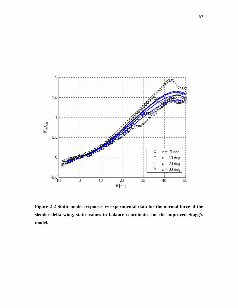
67
Figure 2-2 Static model responses vs experimental data for the normal force of the
slender delta wing, static values in balance coordinates for the improved Stagg’s
model.

68
Figure 2-3 Model responses vs experimental data for the rolling moment coefficient
of the slender delta wing, static values for the improved Stagg’s model.

69
Figure 2-4 Variation of the normal force non-dimensional arms with the roll angle,
static values for the improved Stagg’s model.

70
3 Model Parameters Identifications
3.1 Parameter Identification Method
The identification method used here is the minimum mean-square error approach. The
models have their parameters identified using experimental data in three phases and the
squared error is minimized through an unconstrained optimization process. In the first
two phases, the parameter identification is done using static experimental data. First, we
identify the parameters involved with the determination of the static terms of the normal
lifting forces ( CNxr ). These parameters are those related to the quadratic polynomials that
determine the stability derivatives with respect to the motion variables ( ), and
those that are used to determine the static values of the internal state variables
jjj cba ,,
ix for each
panel i, namely ,∗•)(α )(•σ . Next, we identify only the parameters associated with the arms
of the rolling moment coefficients ( Clxr ) using the experimental static values of the rolling
moment coefficient. In those first two phases of the parameter identification, the
parameters related to the dynamic behavior of the model are kept out of the optimization
process. These dynamic parameters are the coefficients ( ) of the quadratic
polynomials that represent the stability derivatives with respect to the time-rate of the
motion variables, and the time-constant and time-delay parameters, stored in vector
jjj cba ,,
dynxr .
We then take the parameter values previously determined in the two identification phases
described above and use them as initial guess for the third identification phase. In this
third phase, the model parameters are determined when the mean squared error with
respect to dynamic experimental data is minimized for each value of the sting pitch angle.
The dynamic phase of the identification is done using the experimental values of the
rolling moment time histories obtained as described in Section 3.2. Table 3-1 and Table
3-2 show the elements of vectors CNxr , Clxr , and dynxr for the first and the second
investigated models, respectively.

71
When the quasi-static sequences of experimental data are considered, the error cost-
functions to be minimized are as follows,
( ) ( ) ([ ]2
1 100 ,,,ˆ
*1 ∑∑
= =
−=N
j
M
iNCjiNjiNNCCN xCC
NMx rr φθφθε ) (3-1)
( ) ( ) ([ ]∑∑= =
−=j i
lCjiljillCCl xCCNM
x1 1
00 ,,,ˆ*1 rr φθφθε )
N M 2
(3-2)
where each value of the roll angle in the sequence jφ , j = 1,2, ... , N has a corresponding
sequence of values for the wind tunnel sting pitch angle i0θ , i = 1,2, ... , M, as shown in
Figures 1-17 and 1-18. At these points, the wind tunnel measurements are
( ) ( ){ }NjMiCC jiljiN ,...,2,1;,...,2,1;,ˆ,,ˆ00 ==φθφθ , while the model responses determined
at the same points for a given sets NCxr , lCxr of model parameters are
( ) ( ){ }NjMixCxC lCjilNCjiN ,...,2,1;,...,2,1;,,,,, 00 ==rr φθφθ .
When the published values of wind tunnel dynamic measurements at unsteady flow
conditions are used to identify parameters, one roll angle time history ( ){ }Fii Ttt ≤≤0,φ ,
such that FLii Tttttt =<<<<<<= + ......0 121 , is taken for each fixed value of the sting
pitch angle 0θ in the sequence k0θ , k = 1, 2, ... , K . If the corresponding dynamic wind
tunnel measurements of the rolling moment coefficient can be represented by
( )( ){ }KkLitC il ,...,2,1;,...,2,1;,ˆ0 ==θφ and the values of the model responses calculated
at the same points for given set dynxr of model parameters are
( )( ){ KkLixtC il ,...,2,1;,...,2,1;,, 0 == }rθφ , the error cost-function for the dynamic phase
of the identification is
72
( ) ( )( ) ( )( )[ ]2
100 ,,,ˆ1∑
=
−=L
idynilildyndyn xtCtC
Lx rr θφθφε (3-3)
For known sequences of experimental data at each fixed pitch angle 0θ , the design
variables in the cost-functions (3-1) to (3-3) are the model parameters stored in CNxr , Clxr ,
and dynxr . Representing the cost-functions in terms of these model parameters, we have
( )CNCN xrε , ( ClCl xr )ε , and ( )dyndyn xrε . In this particular case, these individual cost-functions
are controlled by different sets of variables, that is, ∗CNxr , ∗
Clxr , ∗dynxr are the solutions to
individual objectives, shown as follows
( ) ( )CNCNCNCN xfx rr ε min, =∗∗
( ) ( )ClClClCl xfxr ε min, =r∗∗
(3-4)
( ) ( )dyndyndyndyn xfxr ε min, =r∗∗
In this research, MATLAB™ scripts have been used to find the values of ( )∗∗CNCNx ε,r ,
( )∗∗ClClx ε,r , and ( )∗∗
dyndynx ε,r . These scripts call the built-in function fminsearch, a
multidimensional unconstrained nonlinear minimization based on the Nelder-Mead
algorithm [56].
Next, we show the experimental data used to identify the model parameters and present
some of the results of the identification.
3.2 Simulated Experimental Data Used in Parameter Identification
Since wind tunnel tests are not part of this research, previously published experimental
data are used to identify the parameters of the investigated models. Because not all the
needed data could be found in just one reference, data from several references are
combined to form the set of simulated experimental data used in the parameter

73
identification. The static data used for the parameter identification are those obtained by
Levin and Katz [47] for the slender delta wing whose geometry is shown in Figure 1-22.
These static experimental data are reproduced in Figure 1-17 and Figure 1-18. Here, it is
assumed that this wing undergoes wing rock for pitch angles between 22 and 45 degrees
of angle of attack. It is also assumed that this wing has a dynamic behavior during steady
state limit cycles similar to the experimental data obtained by Nguyen, Yip, and
Chambers [45] for 0θ = 27 (Figure 1-15) and 32 deg (Figure 1-16). The rolling moment
coefficient experimental histogram for 0θ = 27 deg is also used to identify the model
parameters for 0θ = 38 deg. The rolling moment coefficient experimental histogram for
0θ = 20 deg is also used to identify model parameters for 0θ = 45 deg. All these data are
multiplied by correction factors, to make the maximum absolute values of the rolling
moment coefficient in the cycle consistent with the static value at the same pitch and roll
angles shown in Figure 1-18. For the wing pitch angles at which the oscillations in roll
damp out, the experimental data used to identify the parameters are assumed to have the
same qualitative behavior exhibited in Figure 1-11. At these values of the pitch angle, the
model parameters are identified on the first cycle in roll.
The simulated dynamic experimental data set was extracted from [45] as described next.
The roll angle time history used at angles of attack equal to 27 deg and 38 deg is obtained
from reference [45], and shown in figures 3-13 and 3-16. This roll angle time history was
originally obtained in [45] for the angle of attack equal to 27 deg, where the wing
undergoes wing rock, but it is assumed here to be valid also for an angle of attack of 38
deg. The roll angle time history used for the angles of attack equal to 20 and 45 deg is
shown in figures 3-10 and 3-13. The values of the roll angle φ corresponding to chosen
discrete values of time were taken from these time histories. The corresponding values of
the rolling moment coefficients were taken from the φ×lC plots for each discrete value
of φ . The resulting simulated experimental time histories are shown in figures 3-4, 3-
6, 3-8, 3-11, 3-14, 3-17, and 3-20.
lC

74
3.3 Identification Results
The whole set of model parameters involved in the previously discussed aerodynamic
formulations is stored as vector xr . In order to merge the slender delta wing unsteady
aerodynamic model with the equations of motion and proceed with further analyses, the
models corresponding to the formulations described in Chapter 2 are identified using the
slender delta wing experimental data described in Section 3.2, and the results are
presented in the next Section.
3.3.1 Parameter Identification for the First Investigated Model
The results of the parameter identification of the first investigated model using the static
experimental data are shown from Figure 3-1 to Figure 3-3. Comparing Figure 1-19 and
Figure 3-3, we see that the values of the rolling moment arms vary with the roll angle in
the opposite direction from expectations. The reason for that is that this formulation does
not include the representation of vortex strength and vertical position, which would be
responsible for the pressure distribution surfaces over the wing panels. Therefore, the
restoring rolling moment increases for larger roll angle values is simulated in this
formulation by a bigger moment arm. The remaining parameters identified using static
experimental data are shown on Eqs. (3-5) to (3-7), and in Table 3-4.
Next, the model parameters found for the first investigated model are shown in Equations
(3-5) to (3-22).
( ) ( ) 22-0.005288 iiNiiNNi xCxCC αα
αα ++=
( ) ( ) (3-5) ( ) ˆˆˆ 2iiiNiiNiiN xCxCxC αααα
αααα ˆˆˆ 2 &&&&&&
+++
where:
75
( ) 2 5.427- 7.293-0.6703 iiiN xxxC =α (3-6)
( ) 2 1.838 3.261-1.4532 iiiN xxxC +=α (3-7)
i = left, right panel.
The terms of Eq. (3-5) which are dependent on unsteady aerodynamics have parameters
identified using the rolling moment coefficient experimental time-histories, for one value
of the wing pitch angle at a time. The results of this phase of the identification for the
first investigated model are presented in Figures 3-4 to 3-9. The identified parameters of
the first investigated model at some selected values of the pitch angle θ0 are shown as
follows on Eqs. (3-8) to (3-22):
► 200 =θ deg:
( ) 2 0.005699 761.9-9.656 iiiN xxxC ++=α& (3-8)
( ) 2 0.53422 iiN xxC =α& (3-9)
( ) 0=xC
ˆ
ˆ
(3-10) iN αα &
tx 0.1995,1 =τ (3-11)
t 0.7952,2 =ατ (3-12)
► 270 =θ deg:
( ) 2 0.005660 785.8-10.94 iiiN xxxC ++=α& (3-13)
( ) 2 0.37572 iiN xxC =α& (3-14)
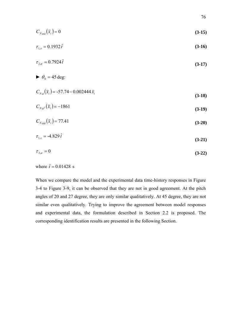
76
( ) 0=xC
ˆ=τ
ˆ
(3-15) iN αα &
(3-16) tx 0.1932,1
t 0.7924,2 =ατ (3-17)
► 450 =θ deg:
( ) iiN xxC 002444.0-57.74−=α& (3-18)
( ) 1861−=xC 2 iNα& (3-19)
( ) =
ˆ
=
41.77iN xC αα & (3-20)
tx 829.4-,1 =τ (3-21)
0,2 ατ (3-22)
where s 01428.0ˆ =t
When we compare the model and the experimental data time-history responses in Figure
3-4 to Figure 3-9, it can be observed that they are not in good agreement. At the pitch
angles of 20 and 27 degree, they are only similar qualitatively. At 45 degree, they are not
similar even qualitatively. Trying to improve the agreement between model responses
and experimental data, the formulation described in Section 2.2 is proposed. The
corresponding identification results are presented in the following Section.

77
Figure 3-1 Static normal force coefficient in balance coordinates vs sting pitch angle.
Model responses (lines) and experimental data (geometric figures) for the improved
Stagg’s model – the first investigated model.
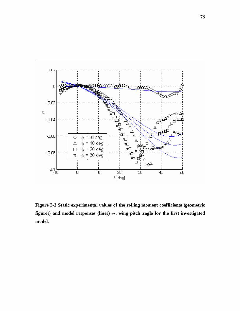
78
Figure 3-2 Static experimental values of the rolling moment coefficients (geometric
figures) and model responses (lines) vs. wing pitch angle for the first investigated
model.
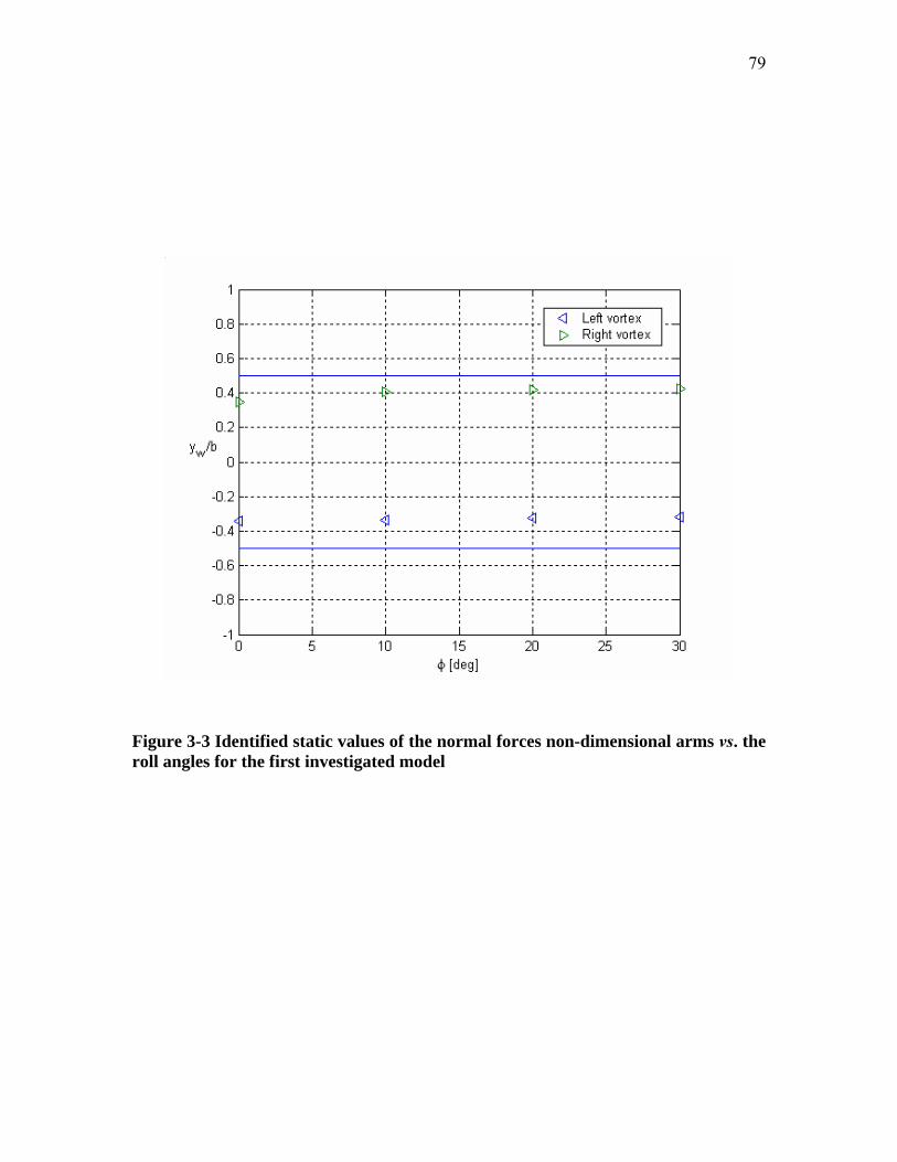
79
Figure 3-3 Identified static values of the normal forces non-dimensional arms vs. the roll angles for the first investigated model

80
Figure 3-4 Rolling moment coefficient time histories for the first investigated model at θ0 = 20 deg.

81
Figure 3-5 Rolling moment coefficient vs. roll angle for the first investigated model at θ0 = 20 deg.

82
Figure 3-6 Rolling moment coefficient time histories for the first investigated model at θ0 = 27 deg.

83
Figure 3-7 Rolling moment coefficient vs. roll angle for the first investigated model at θ0 = 27 deg.

84
Figure 3-8 Rolling moment coefficient time histories for the first investigated model at θ0 = 45 deg.

85
Figure 3-9 Rolling moment coefficient vs. roll angle for the first investigated model at θ0 = 45 deg.

86
3.3.2 Parameter Identification for the Second Investigated Model
In this Section, we present the identification results for the unsteady aerodynamic
formulation described in Section 2.2, when applied to a slender delta wing at angle of
attack and with a degree of freedom only in roll. The identification is done with the help
of the same experimental data set already described on Section 3.2. The sub-sets of
design variables considered in the identification are shown on Table 3-2.
The first try to identify the parameters of the second proposed and investigated
formulation is done by using the procedure exactly as described in Section 3.1 for the
wing at θ0 = 27 degrees, that means that the parameters related to the rolling moment
arms identified using the static experimental data were kept fixed when the dynamic
phase of the identification was made. The results of this first try were not good enough,
probably because the static and dynamic experimental data used in the identifications
come from different sources. In a second try, we left the parameters of the model
parameters vector ∗Clxr free to vary in the dynamic phase of the identification. The results
thus obtained match the experimental data quite well, as can be seen in figures 3-10 to 3-
17. The fact that in this second proposed and investigated unsteady aerodynamic model
we choose internal state variables that are related to physical characteristics of the flow
allows for better insight. Some of the plots of the internal state variables for the wing
pitch angle θ0 = 27 deg are shown in Figure 3-22. According to the identification results
shown in this figure, the vortex breakdown barely goes ahead of the trailing edge. This is
consistent with the experimental observations [46] that show that slender wing rock
happens even when vortex breakdown is not seen over the wing. Figure 3-22 is also
consistent with what is expected for both the y and v internal state variables. We can
see on that figure that the internal state variable y , related to the spanwise positions of
the vortex core, oscillates between the centerline and the half-span. Also on that figure,
the internal state variable related to the vortex strength and vertical position is in phase

87
with the roll angle, and attains its maximum and minimum values at the extreme values
of the roll angle in such a way that the restoring moments keep the oscillations going.
The second model has 62 parameters to be identified, that makes it more capable of
fitting the data. Nevertheless, to find the right set of model parameters is far from
straightforward. If the unconstrained optimization process is carried out for the complete
roll angle time history since the beginning, a good match is hard to achieve. The best
approach is to proceed with the identification starting with a part of the time history, say
one fifth of the whole time history. After good agreement between model response and
simulated experimental data was obtained for that part of the time history, another
fraction was added, and so on. That procedure was used to get the results shown in
figures 3-11 to 3-21. The identified values of the second investigated model parameters
are shown in tables 3-5 to 3-9.

88
0 0.1 0.2 0.3 0.4 0.5 0.6 0.7 0.8 0.9 1-100
-50
0
50
100θ = 20 deg
φ, d
eg
0 0.1 0.2 0.3 0.4 0.5 0.6 0.7 0.8 0.9 110
15
20
25
α, d
eg
time, s
Left wingRight wing
Figure 3-10 Roll angle time history for θ0 = 20 deg (above), and corresponding angle of attack time history for each half-wing (below).

89
0 0.2 0.4 0.6 0.8 1-0.06
-0.04
-0.02
0
0.02
0.04
0.06θ = 20 deg
time, s
Cl
Model responseExperimental data
Figure 3-11 Rolling moment coefficient time-history at θ0 = 20 deg, second investigated model.

90
-60 -40 -20 0 20 40 60-0.06
-0.04
-0.02
0
0.02
0.04
0.06θ = 20 deg
φ, deg
ClModel responseExperimental data
Figure 3-12 Rolling moment coefficient vs. roll angle loops at θ0 = 20 deg, second investigated model.

91
15.6 15.8 16 16.2 16.4 16.6 16.8-40
-20
0
20
40θ = 27 deg
φ, d
eg
15.6 15.8 16 16.2 16.4 16.6 16.822
24
26
28
α, d
eg
time, s
Left wingRight wing
Figure 3-13 Roll angle time history for θ0 = 27 deg (above), and corresponding angle of attack time history for each half-wing (below).

92
15.6 15.8 16 16.2 16.4 16.6 16.8-0.1
-0.05
0
0.05
0.1
0.15θ = 27 deg
time, s
Cl
Model responseExperimental data
Figure 3-14 Rolling moment coefficient time-history at θ0 = 27 deg, second investigated model.

93
-40 -30 -20 -10 0 10 20 30 40-0.1
-0.05
0
0.05
0.1
0.15θ = 27 deg
φ, deg
Cl
Model responseExperimental data
Figure 3-15 Rolling moment coefficient vs. roll angle loops at θ0 = 27 deg.

94
15.6 15.8 16 16.2 16.4 16.6 16.8-40
-20
0
20
40θ = 38 deg
φ, d
eg
15.6 15.8 16 16.2 16.4 16.6 16.832
34
36
38
40
α, d
eg
time, s
Left wingRight wing
Figure 3-16 Roll angle time history for θ0 = 38 deg (above), and corresponding angle of attack time history for each half-wing (below).

95
15.6 15.8 16 16.2 16.4 16.6 16.8-0.1
-0.05
0
0.05
0.1
0.15θ = 38 deg
time, s
Cl
Model responseExperimental data
Figure 3-17 Rolling moment coefficient time-history at θ0 = 38 deg.

96
-40 -30 -20 -10 0 10 20 30 40-0.1
-0.05
0
0.05
0.1
0.15θ = 38 deg
φ, deg
Cl
Model responseExperimental data
Figure 3-18 Rolling moment coefficient vs. roll angle loops at θ0 = 38 deg.
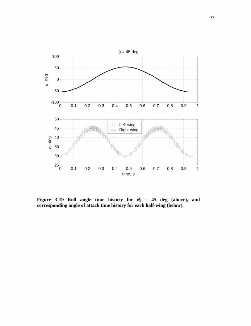
97
0 0.1 0.2 0.3 0.4 0.5 0.6 0.7 0.8 0.9 1-100
-50
0
50
100θ = 45 deg
φ, d
eg
0 0.1 0.2 0.3 0.4 0.5 0.6 0.7 0.8 0.9 125
30
35
40
45
50
α, d
eg
time, s
Left wingRight wing
Figure 3-19 Roll angle time history for θ0 = 45 deg (above), and corresponding angle of attack time history for each half-wing (below).

98
0 0.2 0.4 0.6 0.8 1-0.08
-0.06
-0.04
-0.02
0
0.02
0.04
0.06θ = 45 deg
time, s
Cl
Model responseExperimental data
Figure 3-20 Rolling moment coefficient time-history at θ0 = 45 deg.

99
-60 -40 -20 0 20 40 60-0.08
-0.06
-0.04
-0.02
0
0.02
0.04
0.06θ = 45 deg
φ, deg
Cl
Model responseExperimental data
Figure 3-21 Rolling moment coefficient vs. roll angle loops at θ0 = 45 deg

100
Figure 3-22 Time histories at θ0 = 27 deg of the internal state variables related to the spanwise and vertical positions of the vortices cores.

101
Table 3-1 Model parameters for the first investigated model.
i xCN(i) xCl(i) xdyn(i)
1 CN0 yl @ °= 0φ a3
2 a1 yl @ °= 10φ b3
3 b1 yl @ °= 20φ c3
4 c1 yl @ °= 30φ a4
5 a2 yr @ °= 0φ b4
6 b2 yr @ °= 10φ c4
7 c2 yr @ °= 20φ a5
8 °=∗ 0 @ φαD yr @ °= 30φ b5
9 °=∗ 01 @ φαD - c5
10 °=∗ 02 @ φαD- 1τ
11 °=∗ 03 @ φαD- 2τ
12 °=∗ 0 @ φαU - -
13 °=∗ 01 @ φαU - -
14 °=∗ 02 @ φαU- -
15 °=∗ 03 @ φαU - -
16 °= 0 @ φσ D - -
17 °= 01 @ φσ D - -
18 °= 02 @ φσ D - -
19 °= 03 @ φσ D - -
20 °= 0 @ φσU - -
21 °= 01 @ φσU - -
22 °= 02 @ φσU - -
23 °= 03 @ φσU - -

102
Table 3-2 Model parameters for the second investigated model.
i xCN(i) xCl(i) xdyn(i)
1 CN0 ∗Dly ,,φ a3
2 a1 ∗Uly ,,φ b3
3 b1 Dly ,,σ c3
4 c1 Uly ,,σ a4
5 a2 ∗Dry ,,φ b4
6 b2 ∗Ury ,,φ c4
7 c2 Dry ,,σ a5
8 a6 Ury ,,σ b5
9 b6 - c5
10 c6 - a9
11 a7 - b9
12 b7 - c9
13 c7 - a10
14 a8 - b10
15 b8 - c10
16 c8 - a11
17 ∗Dα - b11
18 ∗Uα - c11
19 Dσ - a12
20 Uσ - b12

103
Table 3-3 Continuation of Table 3-2
i xCN(i) xCl(i) xdyn(i)
21 ∗Dlv ,,φ - c12
22 ∗Ulv ,,φ - x,1τ
23 Dlv ,,σ - y,1τ
24 Ulv ,,σ - v,1τ
25 ∗Drv ,,φ - ατ ,2
26 ∗Urv ,,φ - φτ ,2
27 Drv ,,σ -
28 Urv ,,σ -
Table 3-4 Parameters related to the internal state driving equation location and
slope in function of the roll angle for the first investigated model.
φ
[deg]
∗α σ
0 1.354 4.775
10 1.465 3.660
20 1.543 3.205
30 1.454 3.724

104
Table 3-5 Identified values of the second investigated model parameters stored as xCN
i xCN(i) θ0 = 20 deg θ0 = 27 deg θ0 = 38 deg θ0 = 45 deg
1 CN0 2.7404e-002 2.1850e-002 2.1850e-002 2.7404e-002
2 a1 6.8707e-001 6.8711e-001 6.8711e-001 6.8707e-001
3 b1 -7.0906e+000 -7.0919e+000 -7.0919e+000 -7.0906e+000
4 c1 -5.2137 e+000 -5.2155e+000 -5.2155e+000 -5.2137e+000
5 a2 1.6909 e+000 1.6872e+000 1.6872e+000 1.6909e+000
6 b2 -3.0125 e+000 -3.0145e+000 -3.0145e+000 -3.0125e+000
7 c2 2.1221 e+000 2.1195e+000 2.1195e+000 2.1221e+000
8 a6 -2.6740e-001 -2.2958e-001 -2.2958e-001 -2.6740e-001
9 b6 -2.6043e-002 5.9983e-002 5.9983e-002 -2.6043e-002
10 c6 1.4537e-001 1.7257e-001 1.7257e-001 1.4537e-001
11 a7 8.9613e-003 2.6163e-001 2.6163e-001 8.9613e-003
12 b7 1.2309e-001 1.1374e-001 1.1374e-001 1.2309e-001
13 c7 7.9218e-002 7.9529e-002 7.9529e-002 7.9218e-002
14 a8 1.4662 e+000 9.9747e-002 9.9747e-002 1.4662e+000
15 b8 4.2017e-002 3.9816e-002 3.9816e-002 4.2017e-002
16 c8 2.3602e-002 2.4769e-002 2.4769e-002 2.3602e-002
17 ∗Dα 1.4160e+000 2.8554e+000 3.3317e+000 2.1722e+000
18 ∗Uα 1.4160e+000 2.8554e+000 3.3317e+000 2.1722e+000
19 Dσ 2.0682e+000 1.0377e+001 1.1598e+001 2.8981e+000
20 Uσ 2.0682e+000 1.0377e+001 1.1598e+001 2.8981e+000
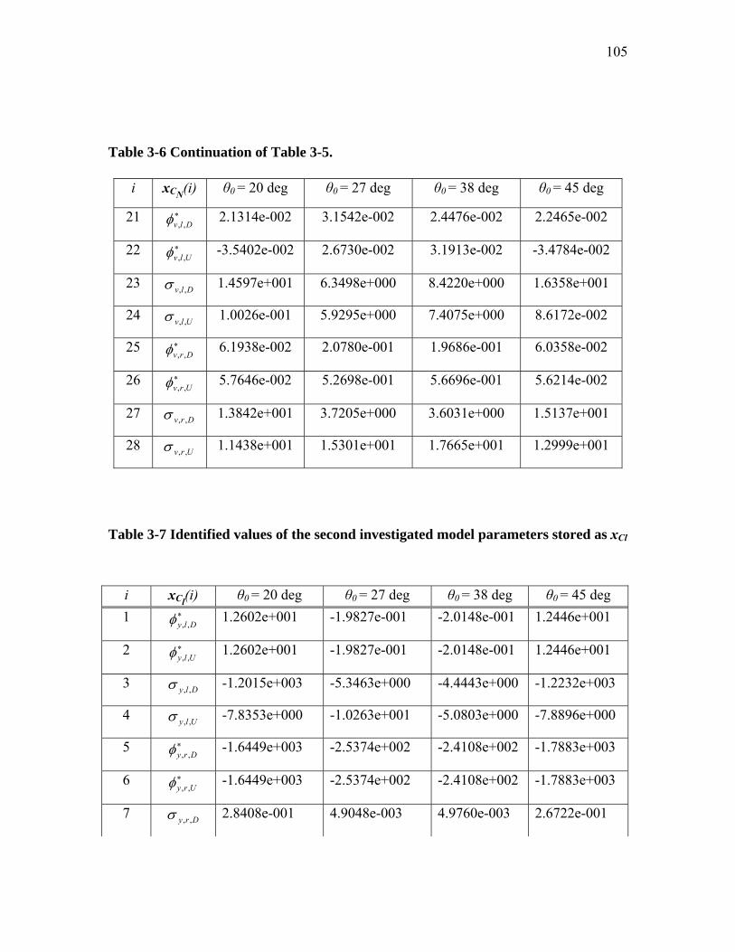
105
Table 3-6 Continuation of Table 3-5.
i xCN(i) θ0 = 20 deg θ0 = 27 deg θ0 = 38 deg θ0 = 45 deg
21 ∗Dlv ,,φ 2.1314e-002 3.1542e-002 2.4476e-002 2.2465e-002
22 ∗Ulv ,,φ -3.5402e-002 2.6730e-002 3.1913e-002 -3.4784e-002
23 Dlv ,,σ 1.4597e+001 6.3498e+000 8.4220e+000 1.6358e+001
24 Ulv ,,σ 1.0026e-001 5.9295e+000 7.4075e+000 8.6172e-002
25 ∗Drv ,,φ 6.1938e-002 2.0780e-001 1.9686e-001 6.0358e-002
26 ∗Urv ,,φ 5.7646e-002 5.2698e-001 5.6696e-001 5.6214e-002
27 Drv ,,σ 1.3842e+001 3.7205e+000 3.6031e+000 1.5137e+001
28 Urv ,,σ 1.1438e+001 1.5301e+001 1.7665e+001 1.2999e+001
Table 3-7 Identified values of the second investigated model parameters stored as xCl
i xCl(i) θ0 = 20 deg θ0 = 27 deg θ0 = 38 deg θ0 = 45 deg 1 ∗
Dly ,,φ 1.2602e+001 -1.9827e-001 -2.0148e-001 1.2446e+001
2 ∗Uly ,,φ 1.2602e+001 -1.9827e-001 -2.0148e-001 1.2446e+001
3 Dly ,,σ -1.2015e+003 -5.3463e+000 -4.4443e+000 -1.2232e+003
4 Uly ,,σ -7.8353e+000 -1.0263e+001 -5.0803e+000 -7.8896e+000
5 ∗Dry ,,φ -1.6449e+003 -2.5374e+002 -2.4108e+002 -1.7883e+003
6 ∗Ury ,,φ -1.6449e+003 -2.5374e+002 -2.4108e+002 -1.7883e+003
7 Dry ,,σ 2.8408e-001 4.9048e-003 4.9760e-003 2.6722e-001

106
8 Ury ,,σ 3.6123e-003 1.3593e-003 1.2434e-003 3.6795e-003
Table 3-8 Identified values of the second investigated model parameters stored as xdyn
i xdyn(i) θ0 = 20 deg θ0 = 27 deg θ0 = 38 deg θ0 = 45 deg
1 a3 -7.1836e-001 -2.6355e+000 -2.3342e+000 -7.2887e-001
2 b3 -1.7830e+002 -8.3922e+001 -7.7390e+001 -1.7330e+002
3 c3 -3.5270e+001 -3.5080e+003 -2.2559e+003 -3.7521e+001
4 a4 2.7081e+002 9.1614e+002 1.3472e+003 2.4691e+002
5 b4 -2.2916e+003 -3.0140e+004 -3.5954e+004 -4.2587e+003
6 c4 -1.6381e+003 -3.5130e+003 -4.8785e+003 -1.7617e+003
7 a5 -4.8981e+002 -2.5102e+001 -1.9191e+001 -1.3918e+002
8 b5 -1.9642e+003 -3.3407e+002 -2.2134e+002 -2.3841e+003
9 c5 -3.2078e+002 -5.9000e+003 -3.8720e+003 -3.3461e+002
10 a9 6.0626e-002 -1.3660e-010 -1.5806e-010 6.3042e-002
11 b9 -6.9690e-011 -1.3880e-010 -1.5829e-010 -7.2307e-011
12 c9 -1.0345e-010 -1.2464e-010 -1.1902e-010 -1.1695e-010
13 a10 -1.8674e+001 -1.2404e-010 -1.4855e-010 -1.9274e+001
14 b10 -1.9758e-011 -6.7498e-011 -9.1097e-011 -1.9740e-011
15 c10 -5.7676e-011 -8.6019e-011 -9.4511e-011 -5.9421e-011
16 a11 6.0378e+001 -1.6238e-010 -1.4520e-010 8.0884e+001
17 b11 -5.5131e-011 -1.0544e-010 -9.6867e-011 -5.5152e-011
18 c11 -8.2905e-011 -1.0210e-010 -1.1436e-010 -9.1052e-011
19 a12 3.4144e-002 -1.3602e-010 -1.7319e-010 3.6664e-002
20 b12 -1.3943e-011 -1.5217e-010 -1.8883e-010 -1.6742e-011

107
Table 3-9 Continuation of Table 3-8
i xdyn(i) θ0 = 20 deg θ0 = 27 deg θ0 = 38 deg θ0 = 45 deg
21 c12 -2.8514e-011 -1.3321e-010 -1.3431e-010 -2.7301e-011
22 x,1τ 2.4910e+001 8.8934e+000 9.4968e+000 3.0446e+001
23 y,1τ 2.4684e+003 4.2317e+001 6.8737e+001 6.1722e+003
24 v,1τ 1.3224e+000 1.0958e+002 1.6284e+002 1.1687e+000
25 ατ ,2 3.0909e+001 4.4349e+001 8.7504e+000 1.6491e+001
26 φτ ,2 1.8651e+000 1.2740e+001 1.1641e+001 1.9255e+000

108
4 Numerical Simulations in Roll
In this Chapter, the single degree of freedom numerical simulation in roll of the slender
delta wing shown on Figure 1-22 is carried out using the second proposed unsteady
aerodynamic model, defined in Section 2.2.
We start by reducing the set of six degree of freedom rigid body equations of motion in
body axes to the simple single degree of freedom pure roll case. Then, we add to the
equations of motion the state and output equations of the unsteady aerodynamic model
and perform some simulations. The six degree of freedom rigid body equations of motion
in body axes are [57]
mXgrvqwu /sin =+−+ θ&
mYgpwruv /sincos =−−+ φθ&
mZgqupvw /coscos =−−+ φθ& (4-1)
( ) ( ) ( ) ( ) LpqrIqprIqrIqrIIpI xzxyyzyyzzxx =+−−+−+−+ &&& 22
( ) ( ) ( ) ( ) MrpIqrpIrpqIprIIqI xzxyyzzzxxyy =−++−−+−+ 22&&&
( ) ( ) ( ) ( ) NpqrIprqIpqIpqIIrI xzyzxyxxyyzz =−+−−−+−+ &&& 22
θψφ sin&& −=p
φθψφθ sincoscos && +=q
φθφθψ sincoscos && −=r
4.1 Rigid Body Dynamics The derivation of the six degree of freedom equations of motion for a rigid body can be
found in several references, for example [4], [58] and [59]. When in body axes
coordinates, they are written as shown in (4-1).
In the case of sting-mounted wind tunnel tests, only the roll degree of freedom is
considered. Then, the body axes components of linear velocity u, v, w, of angular velocity

109
q, r, the Euler angles time rates , θ& ψ& , and their time derivatives are zero. As a
consequence, the general aircraft equations of motion (4-1) are reduced to
LpI xx =& (4-2)
φ&=p
which is a two variable state space system. Here, L stands for the rolling moment
component in body axes.
4.2 Complete Dynamic System
To describe the complete dynamic system, the rigid body system of equations must be
coupled to the unsteady aerodynamic model equations. The aerodynamic model appears
in the rigid body equations (4-1) through the rolling moment coefficient in the system
(4-2), that is:
lxx
CISbqp == φ&&&
As described in Chapter 2 for the second proposed aircraft unsteady aerodynamic model,
the moment coefficients are obtained by multiplying left and right wing force coefficients
by their arms along the corresponding body axis. The complete description of the
functional unsteady aerodynamic formulation (4-2) used is in Section 2.2. In order to
determine the delta wing motion, equations (4-2) must be coupled to equations (2-13),
(2-14), (2-15). The resulting dynamic system built in this way is given by the eight first-
order differential equations (4-3)

110
p=φ&
lxx
CISbqp =&
( ) ( )leffDleffUll
x xDxUxdtxd
,,0,,01 αατ αα +=+
( ) ( )reffDreffUrr
x xDxUxdtxd
,,0,,01 αατ αα +=+
( ) ( )effDleffUlll
y yDyUydtyd
φφτ φφ ,,0,,01 +=+ (4-3)
( ) ( )effDreffUrrr
y yDyUydtyd
φφτ φφ ,,0,,01 +=+
( ) ( )effDleffUlll
v vDvUvdtvd
φφτ φφ ,,0,,01 +=+
( ) ( )effDreffUrrr
v vDvUvdtvd
φφτ φφ ,,0,,01 +=+
The dynamic equations (4-3) must be integrated simultaneously to simulate the slender
delta wing single degree-of-freedom roll motion. The internal state variables ix , iy , iv
are coupled to the two first equations of motion through the rolling moment coefficient
Cl, which is determined by Eq. (2-12), reproduced below for the convenience of the
reader:
( ) ( )φφ rrNllNl yCyCC −= (4-4)
In that equation, the left and right panel normal force coefficients are multiplied by their
arms iy . The normal force coefficients are calculated from the remaining internal state
variables through Eqs. (2-16), (2-29), (2-30), (2-31), and (2-33).

111
4.3 Results of the Simulations
The slender delta wing used in the simulations is wing 2 of Table 1-1. Nevertheless, since
part of the aerodynamic experimental data used to identify the parameters were originally
obtained for wing 1, we took the value of its moment of inertia. Therefore, the mixed
characteristics of the wing used in the simulations are span =b 0.150 m, root chord =rc
0.4285 m, sweep angle at the leading edge 80 degrees, and rolling moment of inertia
= 9.18 kg m
xxI
210−× 2. The air density value adopted for the simulations is =ρ 1.2 kg/m3,
and the airspeed is VT = 9.27 m/s. The first simulation is done for the wing starting from
rest at =0φ 5 deg, =0θ 30 deg. At these conditions, the wing is expected to exhibit wing
rock, and occurs, as Figures 4-1 and 4-2 show. The roll attractor is not located at null roll
angle, as expected from wind tunnel tests like the one whose results are shown on Figure
1-12. Also, the amplitude is much smaller in the present simulations. We attribute this
and other differences between these simulations and the classical wing rock behavior to
the scarcity of the experimental data available to identify the parameters. Figures 4-4 and
4-5 show the results of the simulation starting at =0θ 30 deg, =0φ -5 deg, and 0
deg/s, and we can see that the roll attractor at
=0φ&
=φ -12 deg is confirmed. To better
compare our results to those shown in Figure 1-12, we simulate wing rock with the wing
departing from the roll attractor position. This result shows that the build up time is much
shorter in the present case. Finally, a simulation is started at =0θ 25 deg, and the results
are presented in Figures 4-7 and 4-8. At this pitch angle, wing rock is not supposed to
occur. Results show that it does not in the simulations either, but since the area enclosed
by the loop in Figure 3-12 is so small, the lateral stability of the wing is found to be
practically neutral, and it slowly diverges from the initial position.

112
Figure 4-1 Free to roll simulations at wing pitch angle equal 30 deg, starting at roll angle equal 5 degree.

113
Figure 4-2 Phase-plane of the simulation response at pitch angle equal 30 deg, initial roll angle of 5 degree.

114
Figure 4-3 Free to roll simulations at wing pitch angle equal 30 deg, starting at roll angle equal -5 degree.
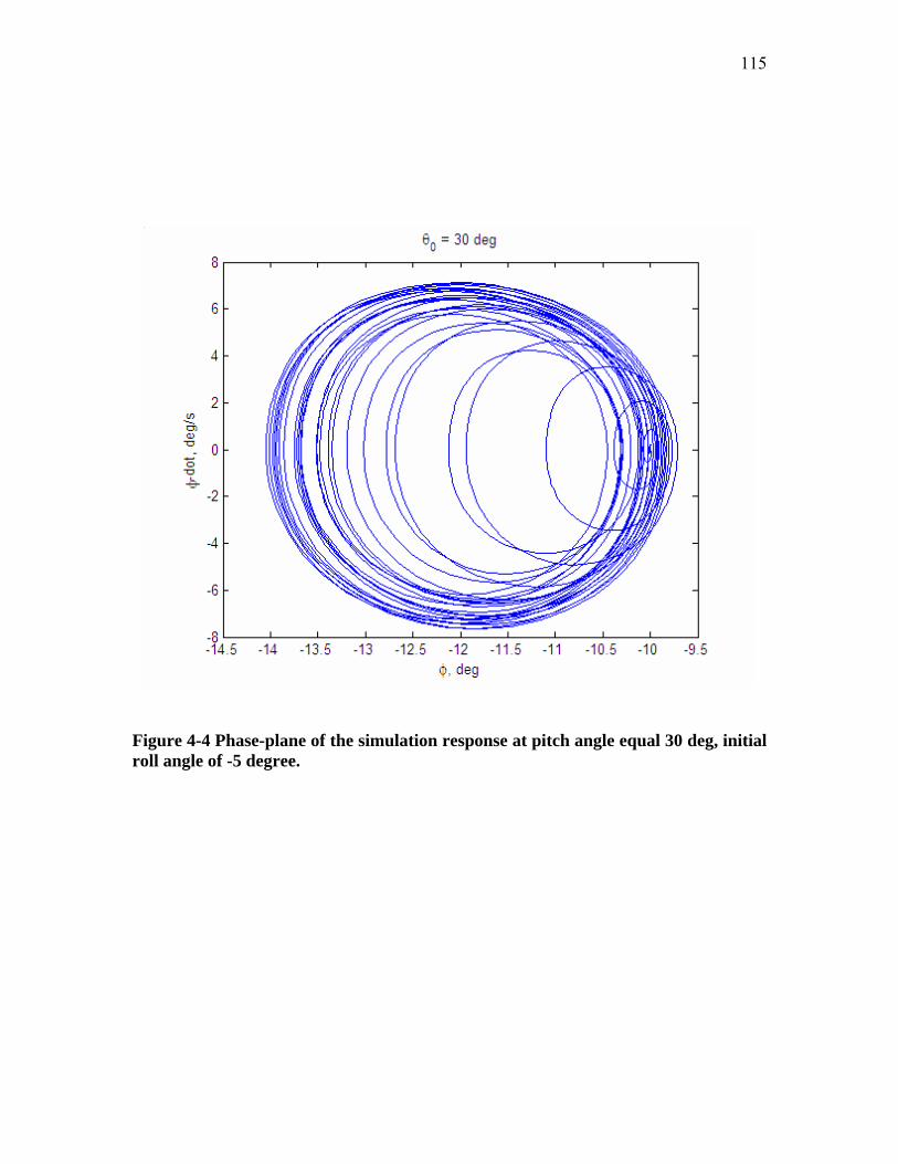
115
Figure 4-4 Phase-plane of the simulation response at pitch angle equal 30 deg, initial roll angle of -5 degree.

116
Figure 4-5 Free to roll simulations at wing pitch angle equal 30 deg, starting at roll angle equal -12 degree.

117
Figure 4-6 Phase-plane of the simulation response at pitch angle equal 30 deg, initial roll angle of -12 degree.
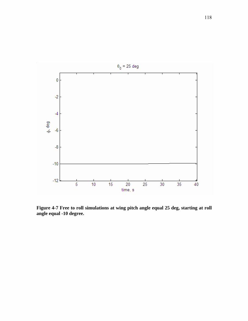
118
Figure 4-7 Free to roll simulations at wing pitch angle equal 25 deg, starting at roll angle equal -10 degree.

119
Figure 4-8 Phase-plane of the simulation response at pitch angle equal 25 deg, initial roll angle of -10 degree.

120
5 Conclusions
Physical models may have a higher computational cost than the functional ones, but their
derivation follows a rationale that is dictated by the physical laws that, like a roadmap,
lead to a logical result. Otherwise, there are theoretically lots of functional models
capable of representing a certain physical phenomenon and this research has shown that
the job of figuring out the one that fits can be daunting. Here, the job of finding one
dynamic functional model with a state-space formulation that represents wing rock was
made a little bit less daunting by following the guidance of physical properties of the
flow observed in previous work. As a result, the second proposed and investigated model
was shown to be capable of representing wing rock even when used with sparse
experimental data. We believe that, with the help of a better set of experimental data,
obtained from the wind tunnel or from computational fluid dynamic programs, far better
results can be reached.
It is opportune to remember that the slender delta wing configuration simulated here was
split into just two panels, and that the simulation is carried out for just one degree of
freedom. According to the results shown in Section 4.2, the application of the proposed
formulation to this kind of problem gives as a result a dynamic system containing two
equations of motion plus six internal state equations for the unsteady aerodynamic model,
making a total of eight first-order differential equations to be simultaneously integrated.
Notice that, if we had a conventional airplane configuration split into six panels to be
simulated in a six degree of freedom motion, the total number of state equations would be
thirty.
In system identification, an appropriate model should have the following characteristics:
(a) to reproduce well enough the plant behavior in the range where the data used to
identify parameters were gathered;
(b) the parameter identification should be easy;
(c) have good ability for generalization.
121
Considering these characteristics, the second model investigated can be considered to be
promising. Its formulation represents the wing rock phenomenon while allowing good
insight into some of the physical properties of the flow. Even though the simultaneous
integration of up to thirty state equations can not be considered low-cost computational
work, it is lower than the computational cost of any physical method.
As future work in this subject is considered, we suggest the use of a physical numerical
method like, for example, the UVLM as a sort of virtual wind tunnel, to get more
consistent simulated experimental data to better identify the proposed model.

122
REFERENCES
[1] Mason, William H., “Stability and Control in Computational Simulations for
Conceptual and Preliminary Design: the Past, Today, and Future?”,
NASA/CP-2004-213028/PT1, Proceedings of a Symposium held in Hampton,
VA, Sept. 23-25, 2003
[2] Juang, J. N., Kholodar, D., and Dowell, E. H., “System Identification of a
Vortex Lattice Aerodynamic Model”, NASA TM-2001-211229, October
2001.
[3] Bryan, G. H., Stability in Aviation, MacMillan, London, 1911.
[4] Etkin, B., Dynamics of Flight – Stability and Control, John Wiley and Sons,
Inc., New York, 1959.
[5] Wagner, H., “Uber die Enstehung des dynamishen Auftriebs von Tragflugen,
Zangew”, Math. U. Mech. 5, pp 17-35., 1925
[6] Theodorsen, T., “General Theory of Aerodynamic Instability and the
Mechanism of Flutter”, NACA TR 496, 1935.
[7] Kussner, H. G., “Zusammenfassender Bericht uber den instationaren Auftrieb
von Flugeln”, Luftfahrtforschung, Bd. 13, Nr. 12, pp 410-424, Dec. 20, 1936.
[8] Cicala, P., “Sul moto non stazionario di un’ala di alungamento finito”, Report
No. 107, Laboratorio di Aeronautica, R. Politecnico di Torino, August 1937.
[9] Jones, R. T., “Operational Treatment of the Non-uniform Lift Theory in
Airplane Dynamics”, NACA TN 667, 1938.

123
[10] Jones, R. T., “The Unsteady Lift of a Wing of Finite Aspect Ratio”, NACA
Rep. 681, June 1939.
[11] Jones, R. T., “The Unsteady Lift of a Finite Wing”, NACA TN 682,
Washington, D.C., January 1939.
[12] Jones, R. T., Fehlner, L. F., “Transient Effects of the Wing Wake on the
Horizontal Tail”, NACA TN 771, 1940.
[13] Tobak, M., “On the Use of the Indicial Function Concept in the Analysis of
Unsteady Motions of Wings and Wing-Tail Combinations”, NACA Report
1188, 1954.
[14] Tobak, M., and Pearson, W. E., “A Study of Nonlinear Longitudinal
Dynamic Stability”, NASA TR R-209, September 1964.
[15] Tobak, M., and Schiff, L. B., “On the Formulation of the Aerodynamic
Characteristics in Aircraft Dynamics”, NASA TR-R-456, 1976.
[16] Tobak, M., Chapman, G. T., Schiff, L. B., “Mathematical Modeling of the
Aerodynamic Characteristics in Flight Dynamics”. NASA TM-85880, Jan.
1984.
[17] Tobak, M., Chapman, G. T., “Nonlinear Problems in Flight Dynamics
Involving Aerodynamic Bifurcations”, NASA-TM-86706, March 1985.
[18] Klein, V., and Noderer, K. D., “Modeling of Aircraft Unsteady Aerodynamic
Characteristics, Part 1 – Postulated Models”, NASA TM 109120, May 1994.

124
[19] Klein, V., and Noderer, K. D., “Modeling of Aircraft Unsteady Aerodynamic
Characteristics, Part 2 – Parameters Estimated From Wind Tunnel Data”,
NASA TM 110161, April 1995.
[20] Klein, V., and Noderer, K. D., “Modeling of Aircraft Unsteady Aerodynamic
Characteristics, Part 3 – Parameters Estimated From Flight Data”, NASA TM
110259, May 1996.
[21] Klein, V., “Modeling of Longitudinal Unsteady Aerodynamics of a Wing-
Tail Combination”, NASA CR-1999-209547, September 1999.
[22] Reisenthel, P. H., “Development of a Nonlinear Indicial Model for
Maneuvering Fighter Aircraft”, AIAA Paper 96-0896, 1996.
[23] Reisenthel, P. H., Bettencourt, M. T., “Data-Based Aerodynamic Modeling
using Nonlinear Indicial Theory”, AIAA Paper 99-0763, 1999.
[24] Reisenthel, P. H., Bettencourt, M. T., “Extraction of Nonlinear Indicial and
Critical States Responses from Experimental Data”, AIAA Paper 99-0764,
1999.
[25] Levinsky, E. S., “Theory of the Wing Span Loading Instabilities Near Stall”,
Paper No. 25, AGARD CP 204, Prediction of Aerodynamic Loading, 1976.
[26] Hreha, M. A., “A Dynamic Model for Aircraft Post-stall Departure”, Ph. D.
Dissertation in Aerospace Engineering, Virginia Polytechnic Institute and
State University, Blacksburg, Virginia, May 1982.
[27] Anderson, M. K., “Aerodynamic Modeling for Global Stability Analysis”,
AIAA Paper 2002-4805, 2002.

125
[28] Goman, M. G., Stolyarov, G. I., Tyrtyshnikov, S. L., Usoltev, S. P., and
Khrabrov, A. N., “Mathematical Description of Aircraft Longitudinal
Aerodynamic Characteristics at High Angles of Attack Accounting for
Dynamic Effects of Separated Flow”, TsAGI Preprint No. 9, 1990 (in
Russian).
[29] Goman, M. and Khrabrov, A., “State-Space Representation of Aerodynamic
Characteristics of an Aircraft at High Angles of Attack”, Journal of Aircraft,
Vol. 31, No. 5, pp. 1109-1115, Sept.-Oct., 1994.
[30] Fan, Y., Lutze, F. H., Identification of an Unsteady Aerodynamic Model at
High Angles of Attack, AIAA Paper 96-3407, 1996.
[31] Abramov, N. B., Goman, M. G., Khrabrov, A. N., Kolinko, K. A., “Simple
Wings Unsteady Aerodynamics at High Angles of Attack: Experimental and
Modeling Results”, AIAA Paper 99-4013, 1999.
[32] De Oliveira Neto, P. J., Lutze, F. H., “First-Order Unsteady Aerodynamic
Model that Includes the Static Hysteresis Penomenon”, AIAA-2002-4083,
Monterey, CA, 2002.
[33] De Oliveira Neto, P. J.; De Almeida, A. R.; Nogueira, S. L.; Verderio, L.; Da
Silva, M. G., “G-Jump Simulations for a Fighter Airplane”, AIAA-2005-
6028, San Francisco, CA, 2005.
[34] Fan, Y., “Identification of an Unsteady Aerodynamic Model up to the High
Angle of Attack Regime”, Ph.D. Dissertation in Aerospace Engineering,
Virginia Polytechnic Institute and State University, Blacksburg, VA, 1994.
[35] Myatt, J. H., “Modeling the Rolling 65-Degree Delta Wing with Critical State
Encounters”, AIAA Paper 97-3646, 1997.
126
[36] Guicheteau, P., “Bifurcation Theory Applied to the Study of Control Losses
on Combat Aircraft”, La Recherche Aerospatiale, 2, pp. 61-73, 1982.
[37] Durham, W., “AOE 3134 Course Notes and Problems Solutions”, Virginia
Polytechnic Institute and State University, Blacksburg, VA, 2004.
[38] von Kárman, T., Sears, W. R., “Airfoil Theory for Non-Uniform Motion”,
Journal of the Aeronautical Sciences, 5(10), 1938
[39] Lutze, F. H., Fan, Y. G., Stagg, G., “Multiaxis Unsteady Aerodynamic
Characteristcs of an Aircraft”, AIAA Paper 99-4011-CP, 1999.
[40] Stagg, G. A., “An Unsteady Aerodynamic Model for Use in the High Angle
of Attack Regime”, M. Sc. Thesis in Aerospace and Ocean Engineering,
Virginia Polytechnic Institute and State University, Blacksburg, Virginia,
Dec., 1998.
[41] USAF Military Specification, “MIL-S-83691A: Stall/Post-Stall/Spin Flight
Test Demonstration Requirements For Airplanes”, April 1972
[42] Abzug, M. J., Larrabee, E. E., Airplane Stability and Control: A History of
the Technologies that made Aviation Possible, Cambridge University Press,
New York, NY, 1997
[43] Hwang, C., Pi, W.S., “Some Observations on the Mechanism of Aircraft
Wing Rock”, Journal of Aircraft, 16(6), 1979
[44] Ross, J. A., Beecham, L. J., “An Approximate Analysis of Nonlinear Lateral
Motion of a Slender Aircraft (HP115) at Low Speed”, ARC&M 3674, 1971.

127
[45] Nguyen, L. T., Yip L., Chambers J. R., “Self-Induced Wing Rock of Slender
Delta Wings”, AIAA Paper 81-1883, AIAA AFM Conference, Albuquerque,
New Mexico, August 1981.
[46] Arena Jr. A., “An Experimental and Computational Investigation of Slender
Wings undergoing Wing Rock”, Ph.D. dissertation, University of Notre
Dame, April 1992.
[47] Levin, D., Katz, J., “Dynamic Load Measurements with Delta Wings
Undergoing Self-Induced Roll Oscillations”, Journal of Aircraft, Vol. 21, No.
1, pp. 30-36, 1984.
[48] Ericson, L. E., “The Various Sources or Wing Rock”, AIAA Paper 88-4370,
August, 1988.
[49] Nguyen, L. T., Whipple, R. D. , and Brandon, J. M., “Recent Experiences of
Unsteady Aerodynamic Effects on Aircraft Flight Dynamics at High-Angles-
of-Attack”, Paper 28, AGARD CP 386, 1985.
[50] Ericson, L. E., “Wing Rock Generated by Forebody Vortices”, AIAA Paper
87-0268, 1987.
[51] Arena Jr., A., “An Experimental Study of the Nonlinear Wing Rock
Phenomenon”, Master´s Thesis, University of Notre Dame, April 1990.
[52] Nelson, R. C., Pelletier, A., “The unsteady aerodynamics of slender wings
and aircraft undergoing large amplitude maneuvers”, Progress in Aerospace
Sciences 39 (2003) 185-248, Elsevier, 2003.
[53] Konstadinopoulos, P., Mook, D. T., Nayfeh, A. H., “Subsonic Wing Rock of
Slender Delta Wings”, Journal of Aircraft, 22(3), pp. 223-228, March 1985.

128
[54] Nayfeh, A. H., Elzebda, J. M., Mook, D. T., “Analytical Study of the
Subsonic Wing-Rock Phenomenon for Slender Delta Wings”, Journal of
Aircraft, Vol. 6, No. 9, September, 1989.
[55] Saad, A. A., “Simulation and Analysis of Wing Rock Physics for a Generic
Fighter Model with Three Degrees-of-Freedom”, Ph.D. Dissertation, Air
Force Institute of Technology, Dayton, Ohio, 2000.
[56] Lagarias, J.C., J. A. Reeds, M. H. Wright, and P. E. Wright, “Convergence
Properties of the Nelder-Mead Simplex Method in Low Dimensions”, SIAM
Journal of Optimization, Vol. 9 Number 1, pp. 112-147, 1998.
[57] Etkin, B., Dynamics of Atmospheric Flight, John Wiley and Sons, Inc. New
York, 1972
[58] Gainer, T.G., and Hoffman, S., “Summary of transformation equations and
equations of motion used in free flight and wind tunnel data reduction and
analysis”, NASA-SP-3070, January 1972
[59] Nelson, R. C., Flight Stability and Automatic Control, 2nd Edition, Mc Graw-
Hill, 1998
[60] Durham, W., “AOE 5214 Course Notes and Problems Solutions”, Virginia
Polytechnic Institute and State University, Blacksburg, VA, 1997.

129
Appendices
Appendix A
A.1 The Convolution Integral Theorem
Also called the Superposition Theorem or Duhamel’s integral theorem [57].
Let to be the Laplace transform of ( )sX1 ( )tx1 , and ( )sX 2 be the transform of ( )tx2 .
Then the function whose transform is the product ( )tx3 ( ) ( ) (sXsXsX 213 )= is
( ) ( ) ( ) ττττ
dtxxtxt
20
13 −= ∫=
The theorem of this section helps with the calculation of transient responses of linear
systems to complicated forcing functions. The general response appears as the
superposition of responses to a sequence of steps or impulses that represent the actual
forcing function.

130
A.2 Angle of attack and sideslip variation during rolling motion at fixed
pitch angle
In a wind tunnel working in steady state conditions, the free stream velocity vector is
constant and horizontal. We therefore choose the X axis of the local horizontal reference
system to be coincident with the velocity vector. When the airplane model rolls around
the sting, the effective angle of attack ( )tα and sideslip ( )tβ in a given time t are related
to the model roll angle ( )tφ at that moment.
The definitions for the angle of attack and sideslip angle as a function of the body-axes
components u, v, and w of the air velocity are [57], [59], [60]:
( )uwt 1tan−=α (A.2-1)
( )222
11
wvuvsin
Vvsint
++== −−β (A.2-2)
The u, v, and w velocity body-axes components can be related to the air velocity through
a local horizontal to the body axis reference systems transformation matrix TB,H, such
that, in the particular case where the heading angle ψ is zero, we have
⎪⎭
⎪⎬
⎫
⎪⎩
⎪⎨
⎧=
⎪⎭
⎪⎬
⎫
⎪⎩
⎪⎨
⎧
00,
VT
wvu
HB (A.2-3)
( ) ( )( ) ( ) ⎥
⎥⎥
⎦
⎤
⎢⎢⎢
⎣
⎡ −
⎥⎥⎥
⎦
⎤
⎢⎢⎢
⎣
⎡=
00
00
,
cos0sin010
sin0cos
cossin-0sincos0
001
θθ
θθ
φφφφ
ttttT HB
( ) ( ) ( )( ) ( ) ( )⎥
⎥⎥
⎦
⎤
⎢⎢⎢
⎣
⎡
−
−=
tttttt
φθφφθφθφφθθθ
coscossincossinsincoscossinsin
sin0cos
00
00
00
(A.2-4)
Therefore,

131
0cosθVu =
φθ sinVsinv 0=
φθ cos0Vsinw = (A.2-5)
Substituting the Eqs. (A.2-5) into the definitions (A.2-1) and (A.2-2), we get
( ) ( )[ ]tt φθα costantan 01−=
( ) ( )[ tt φθβ sin sinsin 01−= ] (A.2-6)
Figure A.2-1 shows the variations of ( )tα and ( )tβ with ( )tφ for °= 200θ . At °= 0φ ,
the model sideslip angle is zero, and its angle of attack is equal 0θ . As the roll angle
grows from 0 to 90 degree, the model angle of attack is reduced to zero and its sideslip
angle grows to the value of the pitch angle.
0 10 20 30 40 50 60 70 80 900
2
4
6
8
10
12
14
16
18
20θ0 = 20 [deg]
Aer
odyn
amic
ang
les,
deg
φ(t), deg
α(t)β(t)
Fig. A.2-1 Variation of the aerodynamic angles with the roll angle for a pure rolling
motion in wind tunnel for pitch angle equal 20 deg.

132
Vita
Pedro Jose de Oliveira Neto was born on February 3rd, 1957 in the small town of
Igarapava - SP, in Brazil. He is the oldest of the three children that Adauto and Laudelina
de Oliveira brought to this world where they no longer live. Since about that time, he has
been fascinated with vehicles, are they traveling in land, sea, air or outer space. This
fascination led him to his Mechanical Engineering B.S. graduation at the Sao Paulo State
University (UNESP), at the Guaratingueta Campus. It also led him to his airplane and
glider pilot licenses. Trying to understand better how these wonderful machines are
conceived, in 1981 he got an internship at the Institute of Aeronautics and Space (IAE),
in Sao Jose dos Campos – SP. Next year, this internship became a full-time job in which
he works since then. As a part of his quest for information, in 1982 he also joined the
Ecole Nationale Superieure de L’Aeronautique et de L’Espace (ENSAE) in Toulouse,
France, where in 1983 he got a Master of Engineering equivalent degree. Trying to
understand how better the aircrafts can be operated, in December of 1996 he got his
Master of Science degree in Flight Dynamics at the Aeronautics Institute of Technology
(ITA), in Sao Jose dos Campos. Trying to know better how to predict and simulate the
behavior of the aircrafts, he joined the Flight Dynamics Group at Virginia Tech, where at
that time people were concerned about traveling to the “left side of the dog’s house”.
Upon receiving his Ph.D. degree in Aerospace in the Fall term of 2007, he will go back to
his work at the Aerodynamics Division of the IAE, in the Aerospace Technology General
Command (CTA). At that time, he is married to Maria, has two children and one
grandchild.