Time Series - CMU Statisticsstat.cmu.edu/~cshalizi/uADA/12/lectures/ch26.pdf · · 2012-05-02Time...

Chapter 26

Time Series

So far, we have assumed that all data points are pretty much independent of eachother. In the chapters on regression, we assumed that each Yi was independent ofevery other, given its Xi , and we often assumed that the Xi were themselves indepen-dent. In the chapters on multivariate distributions and even on causal inference, weallowed for arbitrarily complicated dependence between the variables, but each data-point was assumed to be generated independently. We will now relax this assumption,and see what sense we can make of dependent data.

26.1 Time Series, What They AreThe simplest form of dependent data are time series, which are just what they soundlike: a series of values recorded over time. The most common version of this, instatistical applications, is to have measurements of a variable or variables X at equally-spaced time-points starting from t , written say Xt ,Xt+h ,Xt+2h , . . ., or X (t ),X (t +h),X (t + 2h), . . .. Here h, the amount of time between observations, is called the“sampling interval”, and 1/h is the “sampling frequency” or “sampling rate”.

Figure 26.1 shows two fairly typical time series. One of them is actual data (thenumber of lynxes trapped each year in a particular region of Canada); the other isthe output of a purely artificial model. (Without the labels, it might not be obviouswhich one was which.) The basic idea of all of time series analysis is one which we’realready familiar with from the rest of statistics: we regard the actual time series we seeas one realization of some underlying, partially-random (“stochastic”) process, whichgenerated the data. We use the data to make guesses (“inferences”) about the process,and want to make reliable guesses while being clear about the uncertainty involved.The complication is that each observation is dependent on all the other observations;in fact it’s usually this dependence that we want to draw inferences about.

Other kinds of time series One sometimes encounters irregularly-sampled timeseries, X (t1),X (t2), . . ., where ti − ti−1 �= ti+1 − ti . This is mostly an annoyance,unless the observation times are somehow dependent on the values. Continuously-

495

496 CHAPTER 26. TIME SERIES

Time

lynx

1820 1840 1860 1880 1900 1920

01000

2000

3000

4000

5000

6000

7000

0 20 40 60 80 100

0.0

0.2

0.4

0.6

0.8

1.0

t

y

data(lynx); plot(lynx)

Figure 26.1: Above: annual number of trapped lynxes in the Mackenzie River regionof Canada. Below: a toy dynamical model. (See code online for the toy.)

26.2. STATIONARITY 497

observed processes are rarer — especially now that digital sampling has replaced ana-log measurement in so many applications. (It is more common to model the processas evolving continuously in time, but observe it at discrete times.) We skip both ofthese in the interest of space.

Regular, irregular or continuous time series all record the same variable at everymoment of time. An alternative is to just record the sequence of times at which someevent happened; this is called a “point process”. More refined data might record thetime of each event and its type — a “marked point process”. Point processes includevery important kinds of data (e.g., earthquakes), but they need special techniques,and we’ll skip them.

Notation For a regularly-sampled time series, it’s convenient not to have to keepwriting the actual time, but just the position in the series, as X1,X2, . . ., or X (1),X (2), . . ..This leads to a useful short-hand, that X j

i = (Xi ,Xi+1, . . .Xj−1,Xj ), a whole block oftime; some people write Xi : j with the same meaning.

26.2 Stationarity

In our old IID world, the distribution of each observation is the same as the distribu-tion of every other data point. It would be nice to have something like this for timeseries. The property is called stationarity, which doesn’t mean that the time seriesnever changes, but that its distribution doesn’t.

More precisely, a time series is strictly stationary or strongly stationary whenX k

1 and X t+k−1t have the same distribution, for all k and t — the distribution of

blocks of length k is time-invariant. Again, this doesn’t mean that every block oflength k has the same value, just that it has the same distribution of values.

If there is strong or strict stationarity, there should be weak or loose (or wide-sense) stationarity, and there is. All it requires is that E[X1] = E

�Xt�

, and thatCov�

X1,Xk�= Cov�

Xt ,Xt+k−1�

. (Notice that it’s not dealing with whole blocksof time any more, just single time-points.) Clearly (exercise!), strong stationarityimplies weak stationarity, but not, in general, the other way around, hence the names.It may not surprise you to learn that strong and weak stationarity coincide when Xtis a Gaussian process, but not,in general, otherwise.

You should convince yourself that an IID sequence is strongly stationary.

26.2.1 Autocorrelation

Time series are serially dependent: Xt is in general dependent on all earlier valuesin time, and on all later ones. Typically, however, there is decay of dependence(sometimes called decay of correlations): Xt and Xt+h become more and more nearlyindependent as h→∞. The oldest way of measuring this is the autocovariance,

γ (h) =Cov�

Xt ,Xt+h�

(26.1)


which is well-defined just when the process is weakly stationary. We could equallywell use the autocorrelation,

ρ(h) =Cov�

Xt ,Xt+h�

Var�

Xt� =

γ (h)γ (0)

(26.2)

again using stationarity to simplify the denominator.As I said, for most time series γ (h) → 0 as h grows. Of course, γ (h) could be

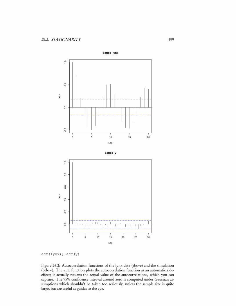
exactly zero while Xt and Xt+h are strongly dependent. Figure 26.2 shows the auto-correlation functions (ACFs) of the lynx data and the simulation model; the correla-tion for the latter is basically never distinguishable from zero, which doesn’t accordat all with the visual impression of the series. Indeed, we can confirm that some-thing is going on the series by the simple device of plotting Xt+1 against Xt (Figure26.3). More general measures of dependence would include looking at the Spearmanrank-correlation of Xt and Xt+h , or quantities like mutual information.

Autocorrelation is important for four reasons, however. First, because it is theoldest measure of serial dependence, it has a “large installed base”: everybody knowsabout it, they use it to communicate, and they’ll ask you about it. Second, in therather special case of Gaussian processes, it really does tell us everything we needto know. Third, in the somewhat less special case of linear prediction, it tells useverything we need to know. Fourth and finally, it plays an important role in acrucial theoretical result, which we’ll go over next.


0 5 10 15 20

-0.5

0.0

0.5

1.0

Lag

ACF

Series lynx

0 5 10 15 20 25 30

0.0

0.2

0.4

0.6

0.8

1.0

Lag

ACF

Series y

acf(lynx); acf(y)

Figure 26.2: Autocorrelation functions of the lynx data (above) and the simulation(below). The acf function plots the autocorrelation function as an automatic side-effect; it actually returns the actual value of the autocorrelations, which you cancapture. The 95% confidence interval around zero is computed under Gaussian as-sumptions which shouldn’t be taken too seriously, unless the sample size is quitelarge, but are useful as guides to the eye.


0 1000 2000 3000 4000 5000 6000 7000

01000

2000

3000

4000

5000

6000

7000

lynxt

lynx

t+1

0.0 0.2 0.4 0.6 0.8 1.0

0.0

0.2

0.4

0.6

0.8

1.0

yt

y t+1

Figure 26.3: Plots of Xt+1 versus Xt , for the lynx (above) and the simulation (below).(See code online.) Note that even though the correlation between successive iteratesis next to zero for the simulation, there is clearly a lot of dependence.


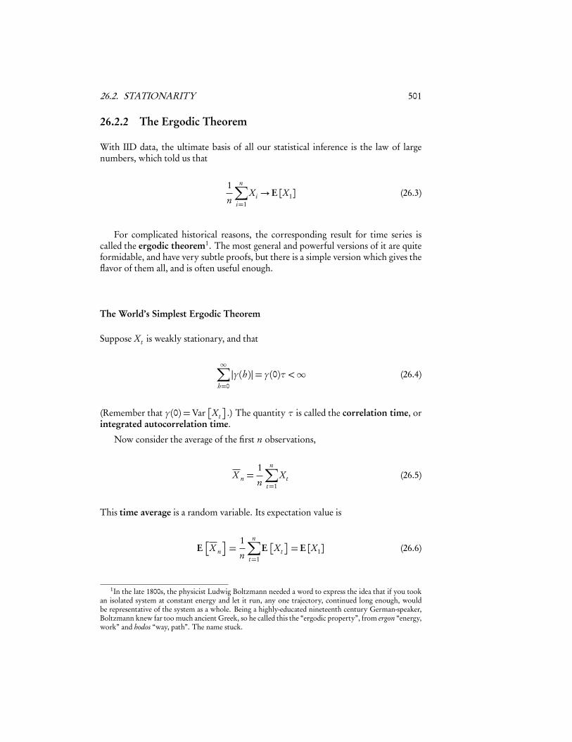
26.2.2 The Ergodic Theorem

With IID data, the ultimate basis of all our statistical inference is the law of largenumbers, which told us that

1n

n�i=1

Xi → E[X1] (26.3)

For complicated historical reasons, the corresponding result for time series iscalled the ergodic theorem1. The most general and powerful versions of it are quiteformidable, and have very subtle proofs, but there is a simple version which gives theflavor of them all, and is often useful enough.

The World’s Simplest Ergodic Theorem

Suppose Xt is weakly stationary, and that

∞�h=0

|γ (h)|= γ (0)τ <∞ (26.4)

(Remember that γ (0) =Var�

Xt�

.) The quantity τ is called the correlation time, orintegrated autocorrelation time.

Now consider the average of the first n observations,

X n =1n

n�t=1

Xt (26.5)

This time average is a random variable. Its expectation value is

E�

X n

�=

1n

n�t=1

E�

Xt�= E[X1] (26.6)

1In the late 1800s, the physicist Ludwig Boltzmann needed a word to express the idea that if you tookan isolated system at constant energy and let it run, any one trajectory, continued long enough, wouldbe representative of the system as a whole. Being a highly-educated nineteenth century German-speaker,Boltzmann knew far too much ancient Greek, so he called this the “ergodic property”, from ergon “energy,work” and hodos “way, path”. The name stuck.


because the mean is stationary. What about its variance?

Var�

X n

�= Var

1

n

n�t=1

Xt

(26.7)

=1

n2

n�t=1

Var�

Xt�+ 2

n�t=1

n�s=t+1

Cov�

Xt ,Xs� (26.8)

=1

n2

nVar[X1]+ 2

n�t=1

n�s=t+1

γ (s − t )

(26.9)

≤ 1

n2

nγ (0)+ 2

n�t=1

n�s=t+1|γ (s − t )| (26.10)

≤ 1

n2

nγ (0)+ 2

n�t=1

n�h=1

|γ (h)| (26.11)

≤ 1

n2

nγ (0)+ 2

n�t=1

∞�h=1

|γ (h)| (26.12)

=nγ (0)(1+ 2τ)

n2 (26.13)

=γ (0)(1+ 2τ)

n(26.14)

Eq. 26.9 uses stationarity again, and then Eq. 26.13 uses the assumption that thecorrelation time τ is finite.

Since E�

Xn

�= E[X1], and Var

�X n

�→ 0, we have that Xn→ E[X1], exactly as

in the IID case. (“Time averages converge on expected values.”) In fact, we can say abit more. Remember Chebyshev’s inequality: for any random variable Z ,

Pr (|Z −E[Z] |> ε)≤ Var[Z]ε2 (26.15)

so

Pr�|X n −E[X1] |> ε

�≤ γ (0)(1+ 2τ)

nε2 (26.16)

which goes to zero as n grows for any given ε.You may wonder whether the condition that

�∞h=0 |γ (h)|<∞ is as weak as pos-

sible. It turns out that it can in fact be weakened to just limn→∞1n

�nh=0 γ (h) = 0, as

indeed the proof above might suggest.

Rate of Convergence

If the Xt were all IID, or even just uncorrelated, we would have Var�

X n

�= γ (0)/n

exactly. Our bound on the variance is larger by a factor of (1+ 2τ), which reflectsthe influence of the correlations. Said another way, we can more or less pretend


that instead of having n correlated data points, we have n/(1+ 2τ) independent datapoints, that n/(1+ 2τ) is our effective sample size2

Generally speaking, dependence between observations reduces the effective sam-ple size, and the stronger the dependence, the greater the reduction. (For an extreme,consider the situation where X1 is randomly drawn, but thereafter Xt+1 = Xt .) Inmore complicated situations, finding the effective sample size is itself a tricky under-taking, but it’s often got this general flavor.

Why Ergodicity Matters

The ergodic theorem is important, because it tells us that a single long time seriesbecomes representative of the whole data-generating process, just the same way thata large IID sample becomes representative of the whole population or distribution.We can therefore actually learn about the process from empirical data.

Strictly speaking, we have established that time-averages converge on expectationsonly for Xt itself, not even for f (Xt ) where the function f is non-linear. It might bethat f (Xt ) doesn’t have a finite correlation time even though Xt does, or indeed viceversa. This is annoying; we don’t want to have to go through the analysis of the lastsection for every different function we might want to calculate.

When people say that the whole process is ergodic, they roughly speaking meanthat

1n

n�t=1

f (X t+k−1t )→ E�

f (X k1 )�

(26.17)

for any reasonable function f . This is (again very roughly) equivalent to

1n

n�t=1

Pr�

X k1 ∈A,X t+l−1

t ∈ B�→ Pr�

X k1 ∈A�

Pr�

X l1 ∈ B�

(26.18)

which is a kind of asymptotic independence-on-average3

If our data source is ergodic, then what Eq. 26.17 tells us is that sample averagesof any reasonable function are representative of expectation values, which is what weneed to be in business statistically. This in turn is basically implied by stationarity.4What does this let us do?

2Some people like to define the correlation time as, in this notation, 1+ 2τ for just this reason.3It’s worth sketching a less rough statement. Instead of working with Xt , work with the whole future

trajectory Yt = (Xt ,Xt+1,Xt+2, . . .). Now the dynamics, the rule which moves us into the future, can besummed up in a very simple, and deterministic, operation T : Yt+1 = T Yt = (Xt+1,Xt+2,Xt+3, . . .). Aset of trajectories is invariant if it is left unchanged by T : for every y ∈ A, there is another y � in A whereT y � = y. A process is ergodic if every invariant set either has probability 0 or probability 1. What thismeans is that (almost) all trajectories generated by an ergodic process belong to a single invariant set, andthey all wander from every part of that set to every other part — they are metrically transitive. (Because:no smaller set with any probability is invariant.) Metric transitivity, in turn, is equivalent, assumingstationarity, to n−1�n−1

t=0 Pr (Y ∈A,T t Y ∈ B)→ Pr (Y ∈A)Pr (Y ∈ B). From metric transitivity followsBirkhoff’s “individual” ergodic theorem, that n−1�n−1

t=0 f (T t Y )→ E[ f (Y )], with probability 1. Since afunction of the trajectory can be a function of a block of length k, we get Eq. 26.17.

4Again, a sketch of a less rough statement. Use Y again for whole trajectories. Every stationarydistribution for Y can be written as a mixture of stationary and ergodic distributions, rather as we wrotecomplicated distributions as mixtures of simple Gaussians in Chapter 20. (This is called the “ergodic


26.3 Markov ModelsFor this section, we’ll assume that Xt comes from a stationary, ergodic time series.So for any reasonable function f , the time-average of f (Xt ) converges on E[ f (X1)].Among the “reasonable” functions are the indicators, so

1n

n�t=1

1A(Xt )→ Pr (X1 ∈A) (26.19)

Since this also applies to functions of blocks,

1n

n�t=1

1A,B (Xt ,Xt+1)→ Pr (X1 ∈A,X2 ∈ B) (26.20)

and so on. If we can learn joint and marginal probabilities, and we remember how todivide, then we can learn conditional probabilities.

It turns out that pretty much any density estimation method which works forIID data will also work for getting the marginal and conditional distributions of timeseries (though, again, the effective sample size depends on how quickly dependencedecays). So if we want to know p(xt ), or p(xt+1|xt ), we can estimate it just as welearned how to do in Chapter 15.

Now, the conditional pdf p(xt+1|xt ) always exists, and we can always estimateit. But why stop just one step back into the past? Why not look at p(xt+1|xt , xt−1),or for that matter p(xt+1|x t

t−999)? There are three reasons, in decreasing order ofpragmatism.

• Estimating p(xt+1|x tt−999) means estimating a thousand-and-one-dimensional

distribution. The curse of dimensionality will crush us.

• Because of the decay of dependence, there shouldn’t be much difference, muchof the time, between p(xt+1|x t

t−999) and p(xt+1|x tt−998), etc. Even if we could

go very far back into the past, it shouldn’t, usually, change our predictions verymuch.

• Sometimes, a finite, short block of the past completely screens off the remotepast.

You will remember the Markov property from your previous probability classes:

Xt+1 |= X t−11 |Xt (26.21)

decomposition” of the process.) We can think of this as first picking an ergodic process according tosome fixed distribution, and then generating Y from that process. Time averages computed along any onetrajectory thus converge according to Eq. 26.17. If we have only a single trajectory, it looks just like astationary and ergodic process. If we have multiple trajectories from the same source, each one may beconverging to a different ergodic component. It is common, and only rarely a problem, to assume that thedata source is not only stationary but also ergodic.

26.3. MARKOV MODELS 505

When the Markov property holds, there is simply no point in looking at p(xt+1|xt , xt−1),because it’s got to be just the same as p(xt+1|xt ). If the process isn’t a simple Markovchain but has a higher-order Markov property,

Xt+1 |= X t−k1 |X t

t−k+1 (26.22)

then we never have to condition on more than the last k steps to learn all that thereis to know. The Markov property means that the current state screens off the futurefrom the past.

It is always an option to model Xt as a Markov process, or a higher-order Markovprocess. If it isn’t exactly Markov, if there’s really some dependence between the pastand the future even given the current state, then we’re introducing some bias, but itcan be small, and dominated by the reduced variance of not having to worry abouthigher-order dependencies.

26.3.1 Meaning of the Markov PropertyThe Markov property is a weakening of both being strictly IID and being strictlydeterministic.

That being Markov is weaker than being IID is obvious: an IID sequence satisfiesthe Markov property, because everything is independent of everything else no matterwhat we condition on.

In a deterministic dynamical system, on the other hand, we have Xt+1 = g (Xt )for some fixed function g . Iterating this equation, the current state Xt fixes thewhole future trajectory Xt+1,Xt+2, . . .. In a Markov chain, we weaken this to Xt+1 =g (Xt , Ut ), where the Ut are IID noise variables (which we can take to be uniform forsimplicity). The current state of a Markov chain doesn’t fix the exact future trajec-tory, but it does fix the distribution over trajectories.

The real meaning of the Markov property, then, is about information flow: thecurrent state is the only channel through which the past can affect the future.


t x1821 2691822 3211823 5851824 8711825 14751826 28211827 39281828 59431829 4950. . .

⇒

lag0 lag1 lag2 lag3871 585 321 2691475 871 585 3212821 1475 871 5853928 2821 1475 8715943 3928 2821 14754950 5943 3928 2821. . .

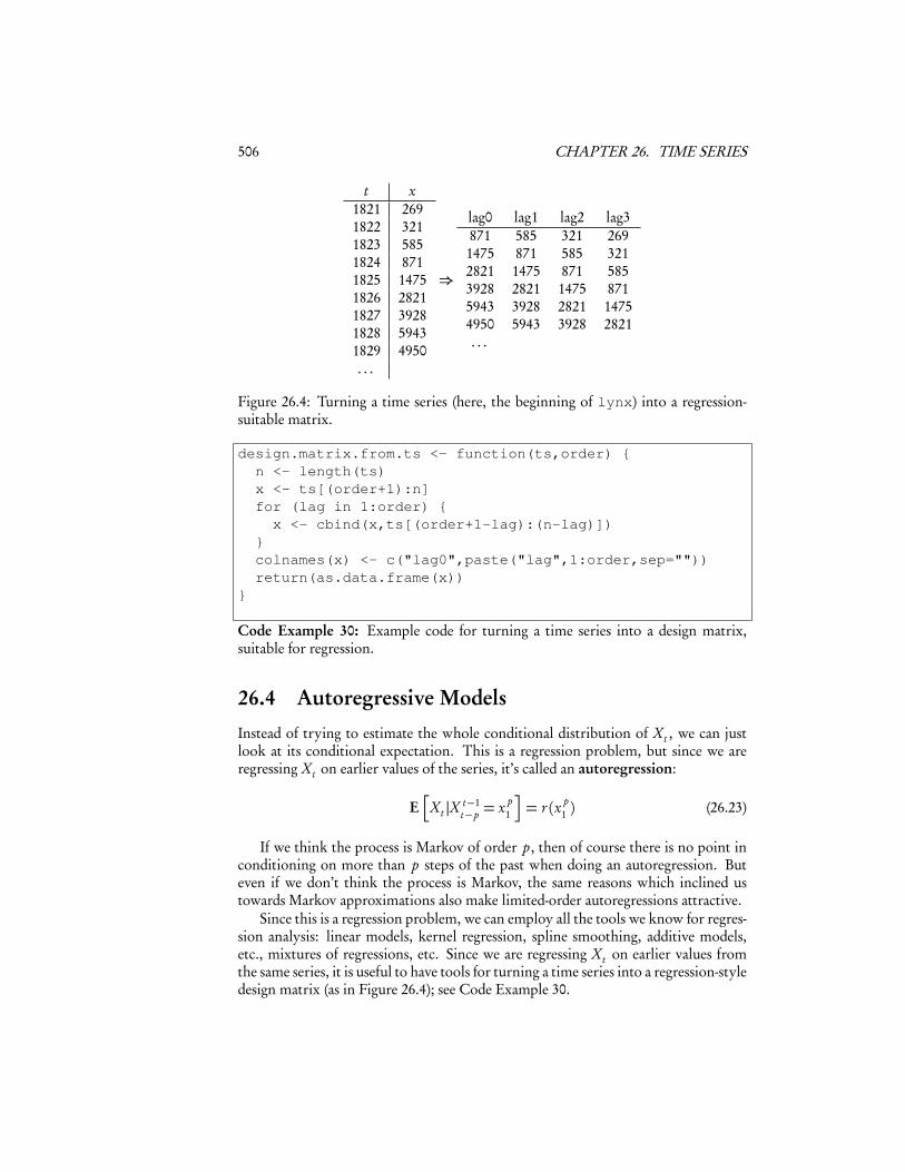
Figure 26.4: Turning a time series (here, the beginning of lynx) into a regression-suitable matrix.

design.matrix.from.ts <- function(ts,order) {n <- length(ts)x <- ts[(order+1):n]for (lag in 1:order) {x <- cbind(x,ts[(order+1-lag):(n-lag)])

}colnames(x) <- c("lag0",paste("lag",1:order,sep=""))return(as.data.frame(x))

}

Code Example 30: Example code for turning a time series into a design matrix,suitable for regression.

26.4 Autoregressive ModelsInstead of trying to estimate the whole conditional distribution of Xt , we can justlook at its conditional expectation. This is a regression problem, but since we areregressing Xt on earlier values of the series, it’s called an autoregression:

E�

Xt |X t−1t−p = x p

1

�= r (x p

1 ) (26.23)

If we think the process is Markov of order p, then of course there is no point inconditioning on more than p steps of the past when doing an autoregression. Buteven if we don’t think the process is Markov, the same reasons which inclined ustowards Markov approximations also make limited-order autoregressions attractive.

Since this is a regression problem, we can employ all the tools we know for regres-sion analysis: linear models, kernel regression, spline smoothing, additive models,etc., mixtures of regressions, etc. Since we are regressing Xt on earlier values fromthe same series, it is useful to have tools for turning a time series into a regression-styledesign matrix (as in Figure 26.4); see Code Example 30.

26.4. AUTOREGRESSIVE MODELS 507

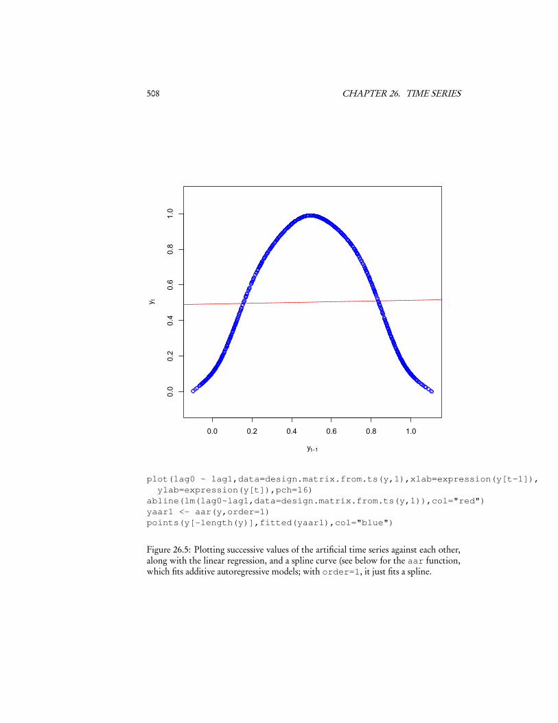
Suppose p = 1. Then we essentially want to draw regression curves through plotslike those in Figure 26.3. Figure 26.5 shows an example for the artificial series.

26.4.1 Autoregressions with CovariatesNothing keeps us from adding a variable other than the past of Xt to the regression:

E�

Xt+1|X tt−k+1,Z�

(26.24)

or even another time series:

E�

Xt+1|X tt−k+1,Z t

t−l+1

�(26.25)

These are perfectly well-defined conditional expectations, and quite estimable in prin-ciple. Of course, adding more variables to a regression means having to estimatemore, so again the curse of dimensionality comes up, but our methods are very muchthe same as in the basic regression analyses.

26.4.2 Additive AutoregressionsAs before, if we want some of the flexibility of non-parametric smoothing, withoutthe curse of dimensionality, we can try to approximate the conditional expectationas an additive function:

E�

Xt |X t−1t−p

�≈ α0+

p�j=1

gj (Xt− j ) (26.26)

Example: The lynx Let’s try fitting an additive model for the lynx. Code Example31 shows some code for doing this. (Most of the work is re-shaping the time seriesinto a data frame, and then automatically generating the right formula for gam.) Let’stry out p = 2.

lynx.aar2 <- aar(lynx,2)

This inherits everything we can do with a GAM, so we can do things like plotthe partial response functions (Figure 26.6), plot the fitted values against the actual(Figure 26.7), etc. To get a sense of how well it can actually extrapolate, Figure 26.8re-fits the model to just the first 80 data points, and then predicts the remaining 34.

26.4.3 Linear AutoregressionWhen people talk about autoregressive models, they usually (alas) just mean linearautoregressions. There is almost never any justification in scientific theory for thispreference, but we can always ask for the best linear approximation to the true au-toregression, if only because it’s fast to compute and fast to converge.


0.0 0.2 0.4 0.6 0.8 1.0

0.0

0.2

0.4

0.6

0.8

1.0

yt!1

y t

plot(lag0 ~ lag1,data=design.matrix.from.ts(y,1),xlab=expression(y[t-1]),ylab=expression(y[t]),pch=16)

abline(lm(lag0~lag1,data=design.matrix.from.ts(y,1)),col="red")yaar1 <- aar(y,order=1)points(y[-length(y)],fitted(yaar1),col="blue")

Figure 26.5: Plotting successive values of the artificial time series against each other,along with the linear regression, and a spline curve (see below for the aar function,which fits additive autoregressive models; with order=1, it just fits a spline.


0 2000 4000 6000

-2000

02000

4000

6000

lag1

0 2000 4000 6000

-2000

02000

4000

6000

lag2

plot(lynx.aar2,pages=1)

Figure 26.6: Partial response functions for the second-order additive autoregressionmodel of the lynx. Notice that a high count last year predicts a higher count thisyear, but a high count two years ago predicts a lower count this year. This is the sortof alternation which will tend to drive oscillations.


Time

lynx

1820 1840 1860 1880 1900 1920

01000

2000

3000

4000

5000

6000

7000

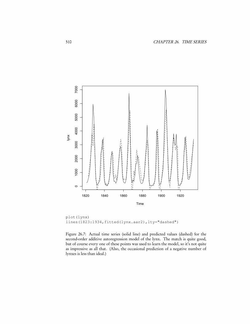
plot(lynx)lines(1823:1934,fitted(lynx.aar2),lty="dashed")

Figure 26.7: Actual time series (solid line) and predicted values (dashed) for thesecond-order additive autoregression model of the lynx. The match is quite good,but of course every one of these points was used to learn the model, so it’s not quiteas impressive as all that. (Also, the occasional prediction of a negative number oflynxes is less than ideal.)


Time

lynx

1820 1840 1860 1880 1900 1920

01000

2000

3000

4000

5000

6000

7000

lynx.aar2b <- aar(lynx[1:80],2)out.of.sample <- design.matrix.from.ts(lynx[-(1:78)],2)lynx.preds <- predict(lynx.aar2b,newdata=out.of.sample)plot(lynx)lines(1823:1900,fitted(lynx.aar2b),lty="dashed")lines(1901:1934,lynx.preds,col="grey")

Figure 26.8: Out-of-sample forecasting. The same model specification as before isestimated on the first 80 years of the lynx data, then used to predict the remaining34 years. Solid black line, data; dashed line, the in-sample prediction on the trainingdata; grey lines, predictions on the testing data. The RMS errors are 723 lynxes/yearin-sample, 922 lynxes/year out-of-sample.


aar <- function(ts,order) {stopifnot(require(mgcv))fit <- gam(as.formula(auto.formula(order)),data=design.matrix.from.ts(ts,order))

return(fit)}

auto.formula <- function(order) {inputs <- paste("s(lag",1:order,")",sep="",collapse="+")form <- paste("lag0 ~ ",inputs)return(form)

}

Code Example 31: Fitting an additive autoregression of arbitrary order to a timeseries. See online for comments.

The analysis we did in Chapter 2 of how to find the optimal linear predictor car-ries over with no change whatsoever. If we want to predict Xt as a linear combinationof the last k observations, Xt−1,Xt−2, . . .Xt−p , then the ideal coefficients β are

β=�

Var�

X t−1t−p

��−1Cov�

X t−1t−p ,Xt

�(26.27)

where Var�

X tt−p

�is the variance-covariance matrix of (Xt−1, . . .Xt−p ) and similarly

Cov�

X t−1t−p ,Xt

�is a vector of covariances. Assume stationarity, Var

�Xt�

is constantin t , and so the common factor of the over-all variance goes away, and β could bewritten entirely in terms of the correlation function ρ. Stationarity also lets us esti-mate these covariances, by taking time-averages.

A huge amount of effort is given over to using linear AR models, which in myopinion is out of all proportion to their utility — but very reflective of what wascomputationally feasible up to about 1980. My experience is that results like Figure26.9 is pretty typical.

“Unit Roots” and Stationary Solutions

Suppose we really believed a first-order linear autoregression,

Xt+1 = α+βXt + εt (26.28)

with εt some IID noise sequence. Let’s suppose that the mean is zero for simplicity,so α= 0. Then

Xt+2 = β2Xt +βεt + εt+1 (26.29)

Xt+3 = β3Xt +β2εt +βεt+1+ εt+2 , (26.30)

etc. If this is going to be stationary, it’d better be the case that what happened attime t doesn’t go on to dominate what happens at all later times, but clearly that


0.0 0.2 0.4 0.6 0.8 1.0

0.0

0.2

0.4

0.6

0.8

1.0

yt!1

y t

library(tseries)yar8 <- arma(y,order=c(8,0))points(y[-length(y)],fitted(yar8)[-1],col="red")

Figure 26.9: Adding the predictions of an eighth-order linear AR model (red dots)to Figure 26.5. We will see the arma function in more detail next time; for now,it’s enough to know that when the second component of its order argument is 0, itestimates and fits a linear AR model.


will happen if |β|> 1, whereas if |β|< 1, eventually all memory of Xt (and εt ) fadesaway. The linear AR(1) model in fact can only produce stationary distributions when|β|< 1.

For higher-order linear AR models, with parameters β1,β2, . . .βp , the corre-sponding condition is that all the roots of the polynomial

p�j=1β j z j − 1 (26.31)

must be outside the unit circle. When this fails, when there is a “unit root”, the linearAR model cannot generate a stationary process.

There is a fairly elaborate machinery for testing for unit roots, which is sometimesalso used to test for non-stationarity. It is not clear how much this really matters. Anon-stationary but truly linear AR model can certainly be estimated5; a linear ARmodel can be non-stationary even if it has no unit roots6; and if the linear model isjust an approximation to a non-linear one, the unit-root criterion doesn’t apply tothe true model anyway.

26.4.4 Conditional VarianceHaving estimated the conditional expectation, we can estimate the conditional vari-ance Var�

Xt |X t−1t−p

�just as we estimated other conditional variances, in Chapter 6.

Example: lynx The lynx series seems ripe for fitting conditional variance functions— presumably when there are a few thousand lynxes, the noise is going to be largerthan when there are only a few hundred.

sq.res <- residuals(lynx.aar2)^2lynx.condvar1 <- gam(sq.res ~ s(lynx[-(1:2)]))lynx.condvar2 <- gam(sq.res ~ s(lag1)+s(lag2),data=design.matrix.from.ts(lynx,2))

I have fit two different models for the conditional variance here, just because.Figure 26.10 shows the data, and the predictions of the second-order additive ARmodel, but with just the standard deviation bands corresponding to the first of thesetwo models; you can try making the analogous plot for lynx.condvar2.

26.4.5 Regression with Correlated Noise; Generalized Least SquaresSuppose we have an old-fashioned regression problem

Yt = r (Xt )+ εt (26.32)

5Because the correlation structure stays the same, even as the means and variances can change. ConsiderXt =Xt−1+ εt , with εt IID.

6Start it with X1 very far from the expected value.


Time

lynx

1820 1840 1860 1880 1900 1920

02000

4000

6000

8000

10000

plot(lynx,ylim=c(-500,10000))sd1 <- sqrt(fitted(lynx.condvar1))lines(1823:1934,fitted(lynx.aar2)+2*sd1,col="grey")lines(1823:1934,fitted(lynx.aar2)-2*sd1,col="grey")lines(1823:1934,sd1,lty="dotted")

Figure 26.10: The lynx data (black line), together with the predictions of the additiveautoregression ±2 conditional standard deviations. The dotted line shows how theconditional standard deviation changes over time; notice how it ticks upwards aroundthe big spikes in population.


only now the noise terms εt are themselves a dependent time series. Ignoring thisdependence, and trying to estimate m by minimizing the mean squared error, is verymuch like ignoring heteroskedasticity. (In fact, heteroskedastic εt are a special case.)What we saw in Chapter 6 is that ignoring heteroskedasticity doesn’t lead to bias,but it does mess up our understanding of the uncertainty of our estimates, and isgenerally inefficient. The solution was to weight observations, with weights inverselyproportional to the variance of the noise.

With correlated noise, we do something very similar. Suppose we knew the co-variance function γ (h) of the noise. From this , we could construct the variance-covariance matrix Γ of the εt (since Γi j = γ (i − j ), of course).

We can use this as follows. Say that our guess about the regression function is m.Stacking y1, y2, . . . yn into a matrix y as usual in regression, and likewise creating m(x),the Gauss-Markov theorem (Appendix C) tells us that the most efficient estimate isthe solution to the generalized least squares problem,

�mGLS = argminm

1n(y−m(x))TΓ−1(y−m(x)) (26.33)

as opposed to just minimizing the mean-squared error,

�mOLS = argminm

1n(y−m(x))T (y−m(x)) (26.34)

Multiplying by the inverse of Γ appropriately discounts for observations which arevery noisy, and discounts for correlations between observations introduced by thenoise.7

This raises the question of how to get γ (h) in the first place. If we knew the trueregression function r , we could use the covariance of Yt − r (Xt ) across different t .Since we don’t know r , but have only an estimate m̂, we can try alternating betweenusing a guess at γ to estimate m̂, and using m̂ to improve our guess at γ . We used thissort of iterative approximation for weighted least squares, and it can work here, too.

7If you want to use a linear model for m, this can be carried through to an explicit modification of theusual ordinary-least-squares estimate — Exercise 1.

26.5. BOOTSTRAPPING TIME SERIES 517

26.5 Bootstrapping Time SeriesThe big picture of bootstrapping doesn’t change: simulate a distribution which isclose to the true one, repeat our estimate (or test or whatever) on the simulation, andthen look at the distribution of this statistic over many simulations. The catch is thatthe surrogate data from the simulation has to have the same sort of dependence as theoriginal time series. This means that simple resampling is just wrong (unless the dataare independent), and our simulations will have to be more complicated.

26.5.1 Parametric or Model-Based BootstrapConceptually, the simplest situation is when we fit a full, generative model — some-thing which we could step through to generate a new time series. If we are confidentin the model specification, then we can bootstrap by, in fact, simulating from thefitted model. This is the parametric bootstrap we saw in Chapter 5.

26.5.2 Block BootstrapsSimple resampling won’t work, because it destroys the dependence between succes-sive values in the time series. There is, however, a clever trick which does work, andis almost as simple. Take the full time series xn

1 and divide it up into overlappingblocks of length k, so xk

1 , xk+12 , . . . xn

n−k+1. Now draw m = n/k of these blocks withreplacement8, and set them down in order. Call the new time series x̃n

1 .Within each block, we have preserved all of the dependence between observa-

tions. It’s true that successive observations are now completely independent, whichgenerally wasn’t true of the original data, so we’re introducing some inaccuracy, butwe’re certainly coming closer than just resampling individual observations (whichwould be k = 1). Moreover, we can make this inaccuracy smaller and smaller byletting k grow as n grows. One can show9 that the optimal k =O(n1/3); this gives agrowing number (O(n2/3)) of increasingly long blocks, capturing more and more ofthe dependence. (We will consider how exactly to pick k in the next chapter.)

The block bootstrap scheme is extremely clever, and has led to a great many vari-ants. Three in particular are worth mentioning.

1. In the circular block bootstrap (or circular bootstrap), we “wrap the time se-ries around a circle”, so that it goes x1, x2, . . . xn1

, xn , x1, x2, . . .. We then samplethe n blocks of length k this gives us, rather than the merely n − k blocks ofthe simple block bootstrap. This makes better use of the information we haveabout dependence on distances < k.

2. In the block-of-blocks bootstrap, we first divide the series into blocks of lengthk2, and then subdivide each of those into sub-blocks of length k1 < k2. Togenerate a new series, we sample blocks with replacement, and then sample

8If n/k isn’t a whole number, round.9I.e., I will not show.


t x1821 2691822 3211823 5851824 8711825 14751826 28211827 39281828 5943

⇒

lag2 lag1 lag0269 321 585321 585 871585 871 1475871 1475 28211475 2821 39282821 3928 5943

⇒lag2 lag1 lag0269 321 585871 1475 2821585 871 1475

⇒

t x̃1821 2691822 3211823 5851824 8711825 14751826 28211827 5851828 871

Figure 26.11: Scheme for block bootstrapping: turn the time series (here, the firsteight years of lynx) into blocks of consecutive values; randomly resample enough ofthese blocks to get a series as long as the original; then string the blocks together inorder. See rblockboot online for code.

sub-blocks within each block with replacement. This gives a somewhat betteridea of longer-range dependence, though we have to pick two block-lengths.

3. In the stationary bootstrap, the length of each block is random, chosen froma geometric distribution of mean k. Once we have chosen a sequence of blocklengths, we sample the appropriate blocks with replacement. The advantageof this is that the ordinary block bootstrap doesn’t quite give us a stationarytime series. (The distribution of X k

k−1 is not the same as the distribution ofX k+1

k.) Averaging over the random choices of block lengths, the stationary

bootstrap does. It tends to be slightly slower to converge that the block orcircular bootstrap, but there are some applications where the surrogate datareally needs to be strictly stationary.

26.5.3 Sieve Bootstrap

A compromise between model-based and non-parametric bootstraps is to use a sievebootstrap. This also simulates from models, but we don’t really believe in them;rather, we just want them to be reasonable easy to fit and simulate, yet flexible enoughthat they can capture a wide range of processes if we just give them enough capacity.

26.5. BOOTSTRAPPING TIME SERIES 519

Time

lynx

1820 1840 1860 1880 1900 1920

01000

2000

3000

4000

5000

6000

7000

plot(lynx)lines(1821:1934, rblockboot(lynx,4),col="grey")

Figure 26.12: The lynx time series, and one run of resampling it with a block boot-strap, block length = 4. (See online for the code to rblockboot.)


We then (slowly) let them get more complicated as we get more data10. One popularchoice is to use linear AR( p) models, and let p grow with n — but there is nothingspecial about linear AR models, other than that they are very easy to fit and simulatefrom. Additive autoregressive models, for instance, would often work at least as well.

26.6 Trends and De-TrendingThe sad fact is that a lot of important real time series are not even approximatelystationary. For instance, Figure 26.13 shows US national income per person (adjustedfor inflation) over the period from 1952 (when the data begins) until now. It is possiblethat this is sample from a stationary process. But in that case, the correlation time isevidently much longer than 50 years, on the order of centuries, and so the theoreticalstationarity is irrelevant for anyone but a very ambitious quantitative historian.

More sensibly, we should try to treat data like this as a non-stationary time series.The conventional approach is o try to separate time series like this into a persistenttrend, and stationary fluctuations (or deviations) around the trend,

Yt = Xt +Zt (26.35)series = fluctuations+ trend

Since we could add or subtract a constant to each Xt without changing whether theyare stationary, we’ll stipulate that E

�Xt�= 0, so E�

Yt�= E�

Zt�

. (In other sit-uations, the decomposition might be multiplicative instead of additive, etc.) Howmight we find such a decomposition?

If we have multiple independent realizations Yi ,t of the same process, say m ofthem, and they all have the same trend Zt , then we can try to find the common trendby averaging the time series:

Zt = E�

Y·,t�≈

m�i=1

Yi ,t (26.36)

Multiple time series with the same trend do exist, especially in the experimental sci-ences. Yi ,t might be the measurement of some chemical in a reactor at time t in the i th

repetition of the experiment, and then it would make sense to average the Yi ,t to getthe common Zt trend, the average trajectory of the chemical concentration. One cantell similar stories about experiments in biology or even psychology, though thoseare complicated by the tendency of animals to get tired and to learn11.

For better or for worse, however, we have only one realization of the post-WWIIUS economy, so we can’t average multiple runs of the experiment together. If wehave a theoretical model of the trend, we can try to fit that model. For instance,

10This is where the metaphor of the “sieve” comes in: the idea is that the mesh of the sieve gets finer andfiner, catching more and more subtle features of the data.

11Even if we do have multiple independent experimental runs, it is very important to get them aligned intime, so that Yi ,t and Yj ,t refer to the same point in time relative to the start of the experiment; otherwise,averaging them is just mush. It can also be important to ensure that the initial state, before the experiment,is the same for every run.

26.6. TRENDS AND DE-TRENDING 521

1950 1960 1970 1980 1990 2000 2010

15000

20000

25000

30000

35000

45000

year

GD

P p

er c

apita

gdppc <- read.csv("gdp-pc.csv")gdppc$y <- gdppc$y*1e6plot(gdppc,log="y",type="l",ylab="GDP per capita")

Figure 26.13: US GDP per capita, constant dollars (consumer price index deflator).Note logarithmic scale of vertical axis. (The values were initially recorded in the filein millions of dollars per person per year, hence the correction.)


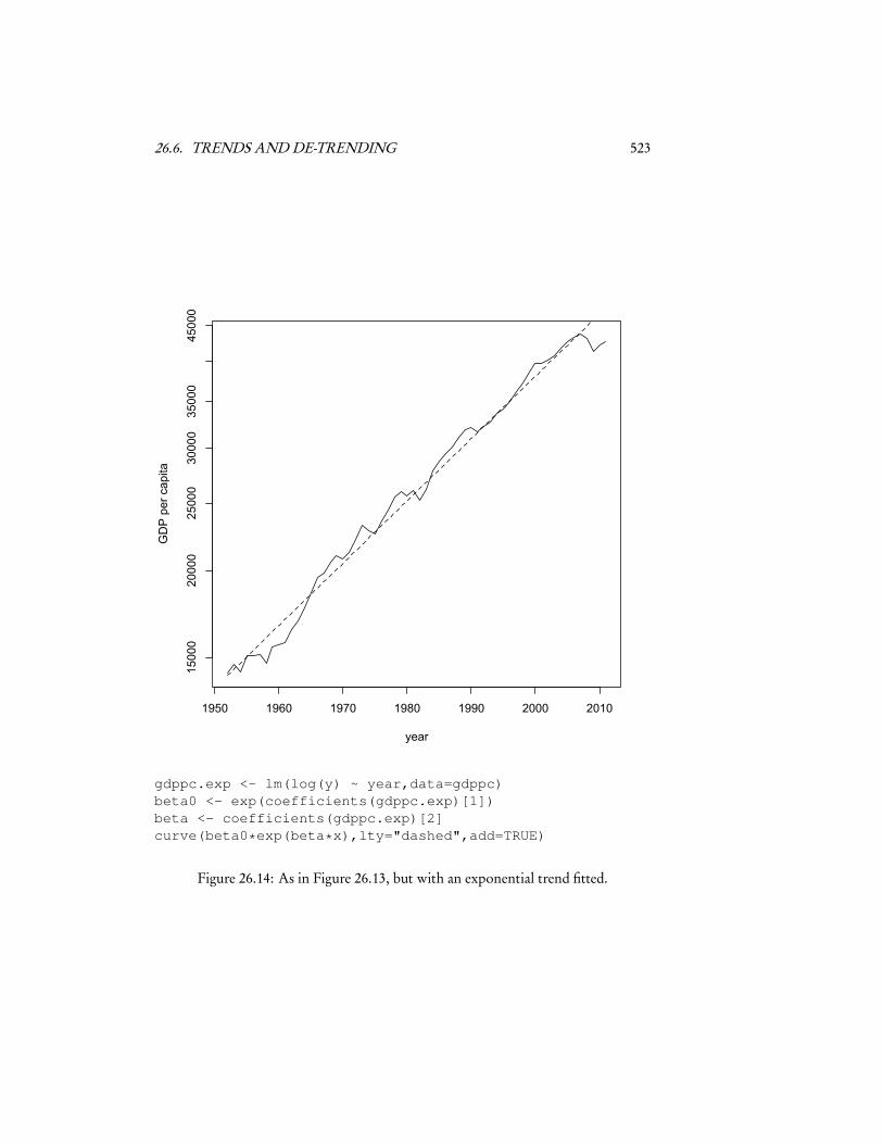
some (simple) models of economic growth predict that series like the one in Figure26.13 should, on average, grow at a steady exponential rate12. We could then estimateZt by fitting a model to Yt of the formβ0eβt , or even by doing a linear regression oflogYt on t . The fluctuations Xt are then taken to be the residuals of this model.

If we only have one time series (no replicates), and we don’t have a good theorywhich tells us what the trend should be, we fall back on curve fitting. In other words,we regress Yt on t , call the fitted values Zt , and call the residuals Xt . This is franklyrests more on hope than on theorems. The hope is that the characteristic time-scalefor the fluctuations Xt (say, their correlation time τ) is short compared to the charac-teristic time-scale for the trend Zt

13. Then if we average Yt over a band-width whichis large compared to τ, but small compared to the scale of Zt , we should get some-thing which is mostly Zt — there won’t be too much bias from averaging, and thefluctuations should mostly cancel out.

Once we have the fluctuations, and are reasonably satisfied that they’re stationary,we can model them like any other stationary time series. Of course, to actually makepredictions, we need to extrapolate the trend, which is a harder business.

26.6.1 Forecasting TrendsThe problem with making predictions when there is a substantial trend is that it isusually hard to know how to continue or extrapolate the trend beyond the last datapoint. If we are in the situation where we have multiple runs of the same process,we can at least extrapolate up to the limits of the different runs. If we have an actualmodel which tells us that the trend should follow a certain functional form, andwe’ve estimated that model, we can use it to extrapolate. But if we have found thetrend purely through curve-fitting, we have a problem.

Suppose that we’ve found the trend by spline smoothing, as in Figure 26.16. Thefitted spline model will cheerfully make predictions for the what the trend of GDPper capita will be in, say, 2252, far outside the data. This will be a simple linear ex-trapolation, because splines are always linear outside the data range (Chapter 7, p.143). This is just because of the way splines are set up, not because linear extrapola-tion is such a good idea. Had we used kernel regression, or any of many other waysof fitting the curve, we’d get different extrapolations. People in 2252 could look backand see whether the spline had fit well, or some other curve would have done better.(But why would they want to?) Right now, if all we have is curve-fitting, we are in adubious position even as regards 2013, never mind 225214

12This is not quite what is claimed by Solow (1970), which you should read anyway if this kind ofquestion is at all interesting to you.

13I am being deliberately vague about what “the characteristic time scale of Zt ” means. Intuitively,it’s the amount of time required for Zt to change substantially. You might think of it as something liken−1�n−1

t=1 1/|Zt+1−Zt |, if you promise not to treat that too seriously. Trying to get an exact statement ofwhat’s involved in identifying trends requires being very precise, and getting into topics at the intersectionof statistics and functional analysis which are beyond the scope of this class.

14Yet again, we hit a basic philosophical obstacle, which is the problem of induction. We have so farevaded it, by assuming that we’re dealing with IID or a stationary probability distribution; these assump-tions let us deductively extrapolate from past data to future observations, with more or less confidence.(For more on this line of thought, see Hacking (2001); Spanos (2011); Gelman and Shalizi (2012).) If we


1950 1960 1970 1980 1990 2000 2010

15000

20000

25000

30000

35000

45000

year

GD

P p

er c

apita

gdppc.exp <- lm(log(y) ~ year,data=gdppc)beta0 <- exp(coefficients(gdppc.exp)[1])beta <- coefficients(gdppc.exp)[2]curve(beta0*exp(beta*x),lty="dashed",add=TRUE)

Figure 26.14: As in Figure 26.13, but with an exponential trend fitted.


1950 1960 1970 1980 1990 2000 2010

-0.10

-0.05

0.00

0.05

year

logg

ed fl

uctu

atio

n ar

ound

tren

d

plot(gdppc$year,residuals(gdppc.exp),xlab="year",ylab="logged fluctuation around trend",type="l",lty="dashed")

Figure 26.15: The hopefully-stationary fluctuations around the exponential growthtrend in Figure 26.14. Note that these are log Yt

β̂0e β̂t, and so unitless.


1950 1960 1970 1980 1990 2000 2010

15000

20000

25000

30000

35000

45000

year

GD

P p

er c

apita

gdp.spline <- fitted(gam(y~s(year),data=gdppc))lines(gdppc$year,gdp.spline,lty="dotted")

Figure 26.16: Figure 26.14, but with the addition of a spline curve for the time trend(dotted line). This is, perhaps unsurprisingly, not all that different from the simpleexponential-growth trend.


1950 1960 1970 1980 1990 2000 2010

-0.10

-0.05

0.00

0.05

year

logg

ed fl

uctu

atio

n ar

ound

tren

d

lines(gdppc$year,log(gdppc$y/gdp.spline),xlab="year",ylab="logged fluctuations around trend",lty="dotted")

Figure 26.17: Adding the logged deviations from the spline trend (dotted) to Figure26.15.


26.6.2 Seasonal ComponentsSometimes we know that time series contain components which repeat, pretty ex-actly, over regular periods. These are called seasonal components, after the obviousexample of trends which cycle each year with the season. But they could cycle overmonths, weeks, days, etc.

The decomposition of the process is thus

Yt =Xt +Zt + St (26.37)

where Xt handles the stationary fluctuations, Zt the long-term trends, and St therepeating seasonal component.

If Zt = 0, or equivalently if we have a good estimate of it and can subtract it out,we can find St by averaging over multiple cycles of the seasonal trend. Suppose thatwe know the period of the cycle is T , and we can observe m = n/T full cycles. Then

St ≈1m

m−1�j=0

Yt+ j T (26.38)

This works because, with Zt out of the picture, Yt = Xt + St , and St is periodic,St = St+T . Averaging over multiple cycles, the stationary fluctuations tend to cancelout (by the ergodic theorem), but the seasonal component does not.

For this trick to work, we need to know the period. If the true T = 355, but weuse T = 365 without thinking15, we can get mush.

We also need to know the over-all trend. Of course, if there are seasonal compo-nents, we really ought to subtract them out before trying to find Zt . So we have yetanother vicious cycle, or, more optimistically, another case for iterative approxima-tion.

26.6.3 Detrending by DifferencingSuppose that Yt has a linear time trend:

Yt =β0+βt +Xt (26.39)

with Xt stationary. Then if we take the difference between successive values of Yt ,the trend goes away:

Yt −Yt−1 =β+Xt −Xt−1 (26.40)

Since Xt is stationary,β+Xt−Xt−1 is also stationary. Taking differences has removedthe trend.

Differencing will not only get rid of linear time trends. Suppose that

Zt = Zt−1+ εt (26.41)

assume a certain form or model for the trend, then again we can deduce future behavior on that basis. Butif we have neither probabilistic nor mechanistic assumptions, we are, to use a technical term, stuck withinduction. Whether there is some principle which might help — perhaps a form of Occam’s Razor (Kelly,2007)? — is a nice question.

15Exercise: come up with an example of a time series where the periodicity should be 355 days.


where the “innovations” or “shocks” εt are IID, and that

Yt = Zt +Xt (26.42)

with Xt stationary, and independent of the εt . It is easy to check that (i) Zt is notstationary (Exercise 2), but that (ii) the first difference

Yt −Yt−1 = εt +Xt −Xt−1 (26.43)

is stationary. So differencing can get rid of trends which are built out of the summa-tion of persistent random shocks.

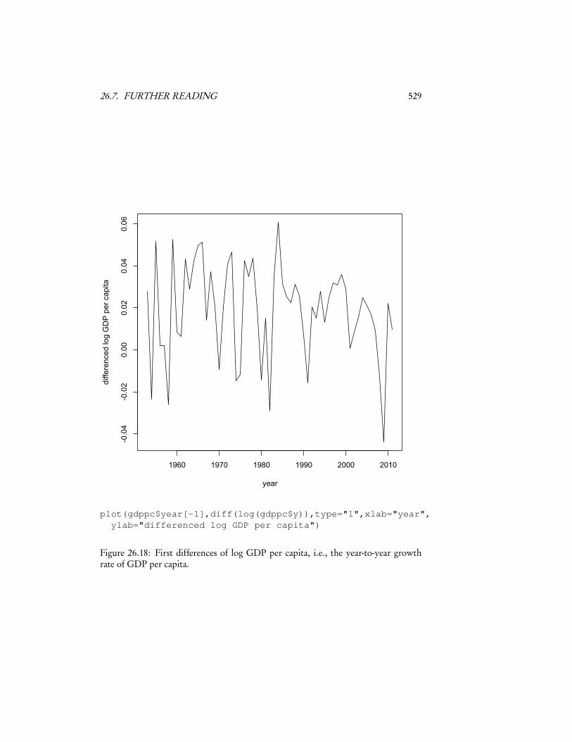
This gives us another way of making a time series stationary: instead of trying tomodel the time trend, take the difference between successive values, and see if that isstationary. (The diff() function in R does this; see Figure 26.18.) If such “first dif-ferences” don’t look stationary, take differences among differences, third differences,etc., until you have something satisfying.

Notice that now we can continue to the trend: once we predict Yt+1−Yt , we addit on to Yt (which we observed) to get Yt+1.

Differencing is like taking the discrete version of a derivative. It will eventuallyget rid of trends if they correspond to curves (e.g., polynomials) with only finitelymany non-zero derivatives. It fails for trends which aren’t like that, like exponentialsor sinusoids, though you can hope that eventually the higher differences are smallenough that they don’t matter much.

26.7 Further ReadingShumway and Stoffer (2000) is a good introduction to conventional time series anal-ysis, covering R practicalities. Lindsey (2004) surveys a broader range of situations inless depth; it is readable, but opinionated, and I don’t always agree with the opinions.Fan and Yao (2003) is a deservedly-standard reference on nonparametric time seriesmodels. The theoretical portions would be challenging for most readers of this book,but the methodology isn’t, and it devotes about the right amount of space (no morethan a quarter of the book) to the usual linear-model theory.

The block bootstrap was introduced by Künsch (1989). Davison and Hinkley(1997, §8.2) has a characteristically-clear treatment of the main flavors of bootstrapfor time series; Lahiri (2003) is a thorough but theoretical. Bühlmann (2002) is alsouseful.

The best introduction to stochastic processes I know of, by a very wide mar-gin, is Grimmett and Stirzaker (1992). However, like most textbooks on stochasticprocesses, it says next to nothing about how to use them as models of data. Two ex-ceptions I can recommend are the old but insightful Bartlett (1955), and the excellentGuttorp (1995).

The basic ergodic theorem in §26.2.2 follows a continuous-time argument inFrisch (1995). My general treatment of ergodicity is heavily shaped by Gray (1988)and Shields (1996).

In parallel to the treatment of time series by statisticians, physicists and mathe-maticians developed their own tradition of time-series analysis (Packard et al., 1980),

26.7. FURTHER READING 529

1960 1970 1980 1990 2000 2010

-0.04

-0.02

0.00

0.02

0.04

0.06

year

diffe

renc

ed lo

g G

DP

per

cap

ita

plot(gdppc$year[-1],diff(log(gdppc$y)),type="l",xlab="year",ylab="differenced log GDP per capita")

Figure 26.18: First differences of log GDP per capita, i.e., the year-to-year growthrate of GDP per capita.


where the basic models are not stochastic processes but deterministic, yet unstable,dynamical systems. Perhaps the best treatment of this are Abarbanel (1996); Kantzand Schreiber (2004). There are in fact very deep connections between this approachand the question of why probability theory works in the first place (Ruelle, 1991),but that’s not a subject for data analysis.

26.8 Exercises1. In Eq. 26.33, assume that m(x) has to be a linear function, m(x) =β · x. Solve

for the optimalβ in terms of y, x, and Γ. This “generalized least squares” (GLS)solution should reduce to ordinary least squares when Γ= σ2I.

2. If Zt = Zt−1 + εt , with εt IID, prove that Zt is not stationary. Hint: considerVar�

Zt�

.

Time Series - CMU Statisticsstat.cmu.edu/~cshalizi/uADA/12/lectures/ch26.pdf · · 2012-05-02Time...

Documents

Transcript of Time Series - CMU Statisticsstat.cmu.edu/~cshalizi/uADA/12/lectures/ch26.pdf · · 2012-05-02Time...