Midterm Examination

36-350, Data Mining

14 October 2009

No notes or calculators are allowed. All calculations can be done by hand,possibly (but not necessarily) using the facts on this page. SHOW YOURWORK: partial credit will be based on work; correct answers without workwill receive minimal or no credit. If you suspect you have made a mistake butcannot find it, say so, and say why you think there is an error.

Problem Points1 152 353 254 25

Possibly Helpful Facts

here, x is an m× 1 matrix and A and B are m×m

dxT xdx

= 2x

dxT Axdx

= Ax + AT x

Ax = vx ⇔ x is an eigenvector of A with eigenvalue v

(AB)T = BT AT

1

1. (15 points in all) Briefly define the following terms (2 pt each). Formulasare OK, but explain what the symbols in them mean.

(a) Ward’s method (of clustering)

(b) Entropy

(c) Inverse document frequency

(d) Cross-validation

(e) Nearest neighbor classifier

(f) Dendrogram

(g) Confusion matrix

2

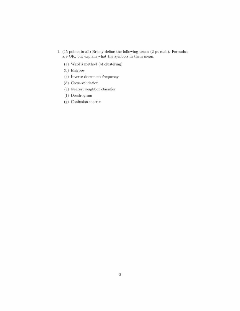
2. Finding reviewers (35 pts total) Scientific papers submitted to a journal orconference are “peer-reviewed”, meaning that they are evaluated by otherscientists familiar with work in the area. Journal editors and conferenceorganizers spend a lot of time selecting reviewers, and authors worry aboutgetting good referees.

Suppose that a journal has a database of the full text of all papers previ-ously published in the journal, along with their authors.

(a) (3 pts) Explain what the bag-of-words representation for an individ-ual paper would be.

(b) (2 pts) Explain how to combine the representations of all papers bya given author to get a bag-of-words for that author.

(c) (15 pts) Describe an algorithm for finding the three authors whosework is most relevant to a given paper, and are not authors of thepaper. (You do not have to write code, but be clear about whatneeds to be done.)

(d) (5 pts) How could you use principal components analysis of bags ofwords to simplify and improve this system?

(e) (5 pts) Describe how to use the bags-of-words to hierarchically clusterauthors.

(f) (5 pts) Describe another algorithm for finding peer reviewers of apaper, using the hierarchical clustering of authors.

3

3. (25 points in all) state.x77 is a data set about the United States in 1977,using figures taken from the Census’s Statistical Abstract. (You will seethis again in the homework.) The variables are:

Population in thousandsIncome dollars per capitaIlliteracy Percent of the adult population unable to read and writeLife Exp Average years of life expectancy at birthMurder Number of murders and non-negligent manslaughters per 100,000 peopleHS Grad Percent of adults who were high-school graduatesFrost Mean number of days per year with low temperatures below freezingArea In square miles

The summary statistics for these variables will be helpful.

> summary(state.x77)Population Income Illiteracy Life Exp

Min. : 365 Min. :3098 Min. :0.500 Min. :67.961st Qu.: 1080 1st Qu.:3993 1st Qu.:0.625 1st Qu.:70.12Median : 2838 Median :4519 Median :0.950 Median :70.67Mean : 4246 Mean :4436 Mean :1.170 Mean :70.883rd Qu.: 4968 3rd Qu.:4814 3rd Qu.:1.575 3rd Qu.:71.89Max. :21198 Max. :6315 Max. :2.800 Max. :73.60

Murder HS Grad Frost AreaMin. : 1.400 Min. :37.80 Min. : 0.00 Min. : 10491st Qu.: 4.350 1st Qu.:48.05 1st Qu.: 66.25 1st Qu.: 36985Median : 6.850 Median :53.25 Median :114.50 Median : 54277Mean : 7.378 Mean :53.11 Mean :104.46 Mean : 707363rd Qu.:10.675 3rd Qu.:59.15 3rd Qu.:139.75 3rd Qu.: 81162Max. :15.100 Max. :67.30 Max. :188.00 Max. :566432

We will do two different principal component analyses of this data.

> states.pca.1 = prcomp(state.x77,scale.=FALSE)> states.pca.2 = prcomp(state.x77,scale.=TRUE)

The figures following show some displays for these two PCAs, which youwill need to use to answer the questions.

4

-0.4 -0.2 0.0 0.2 0.4 0.6 0.8

-0.4

-0.2

0.0

0.2

0.4

0.6

0.8

PC1

PC2

Alabama

AlaskaArizonaArkansas

California

ColoradoConnecticut

Delaware

Florida

Georgia

HawaiiIdaho

Illinois

IndianaIowaKansasKentuckyLouisiana

Maine

MarylandMassachusetts

Michigan

MinnesotaMississippi

Missouri

MontanaNebraskaNevadaNew Hampshire

New Jersey

New Mexico

New York

North Carolina

North Dakota

Ohio

OklahomaOregon

Pennsylvania

Rhode IslandSouth Carolina

South Dakota

Tennessee

Texas

UtahVermont

VirginiaWashington

West Virginia

Wisconsin

Wyoming

-4e+05 -2e+05 0e+00 2e+05 4e+05 6e+05

-4e+05

-2e+05

0e+00

2e+05

4e+05

6e+05

PopulationIncomeIlliteracyLife ExpMurderHS GradFrost Area

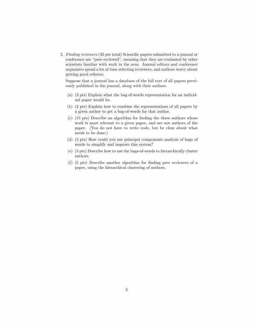
Figure 1: Biplot for states.pca.1.

PC1 PC2Population 1.18× 10−03 −1.00Income 2.62× 10−3 −2.80× 10−2

Illiteracy 5.52× 10−7 −1.42× 10−5

Life Exp −1.69× 10−6 1.93× 10−5

Murder 9.88× 10−6 −2.79× 10−4

HS Grad 3.16× 10−5 1.88× 10−4

Frost 3.61× 10−5 3.87× 10−3

Area 1.00 1.26× 10−3

Table 1: Projections of the features on to the first two principal components ofstates.pca.1.

5

0e+00 1e+05 2e+05 3e+05 4e+05 5e+05

-15000

-10000

-5000

05000

PC1

PC2

AL

AK

AZAR

CA

COCT

DE

FL

GA

HI ID

IL

IN

IAKS

KYLA

ME

MD

MA

MI

MN

MS

MO

MTNE

NVNH

NJ

NM

NY

NC

ND

OH

OKOR

PA

RI

SC

SD

TN

TX

UTVT

VA

WA

WV

WI

WY

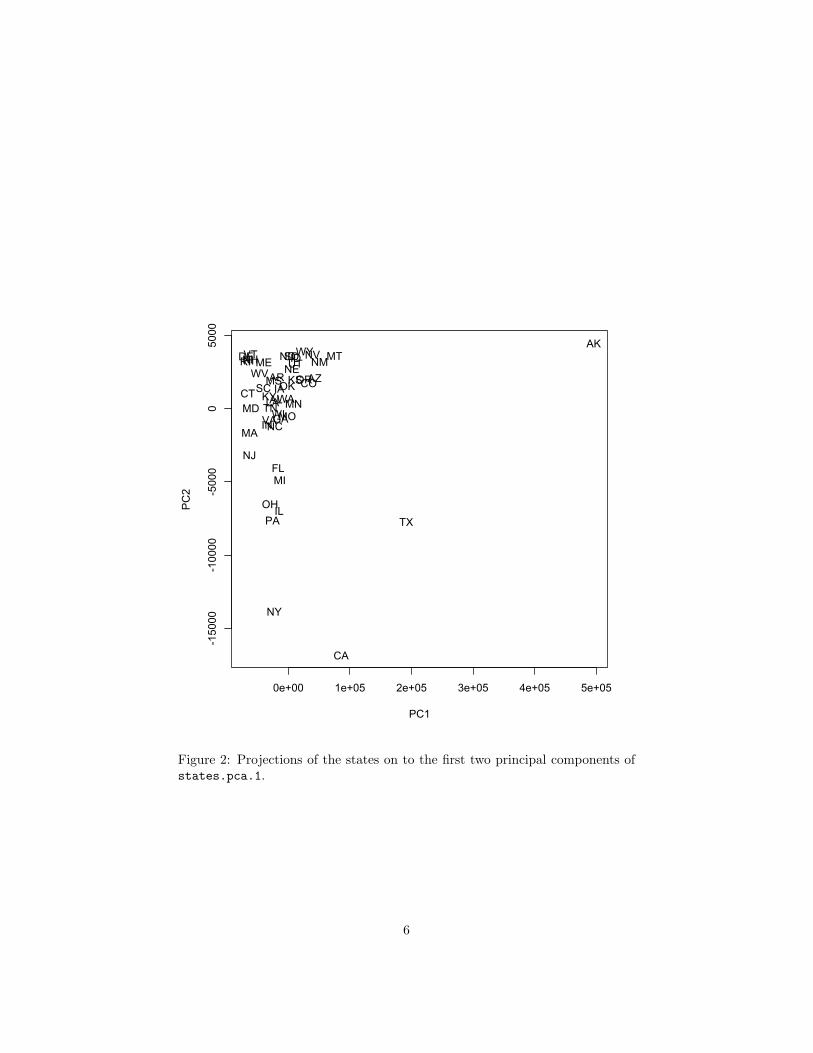
Figure 2: Projections of the states on to the first two principal components ofstates.pca.1.

6

states.pca.1

scree plot

Variances

0e+00

2e+09

4e+09

6e+09

1 2 3 4 5 6 7 8

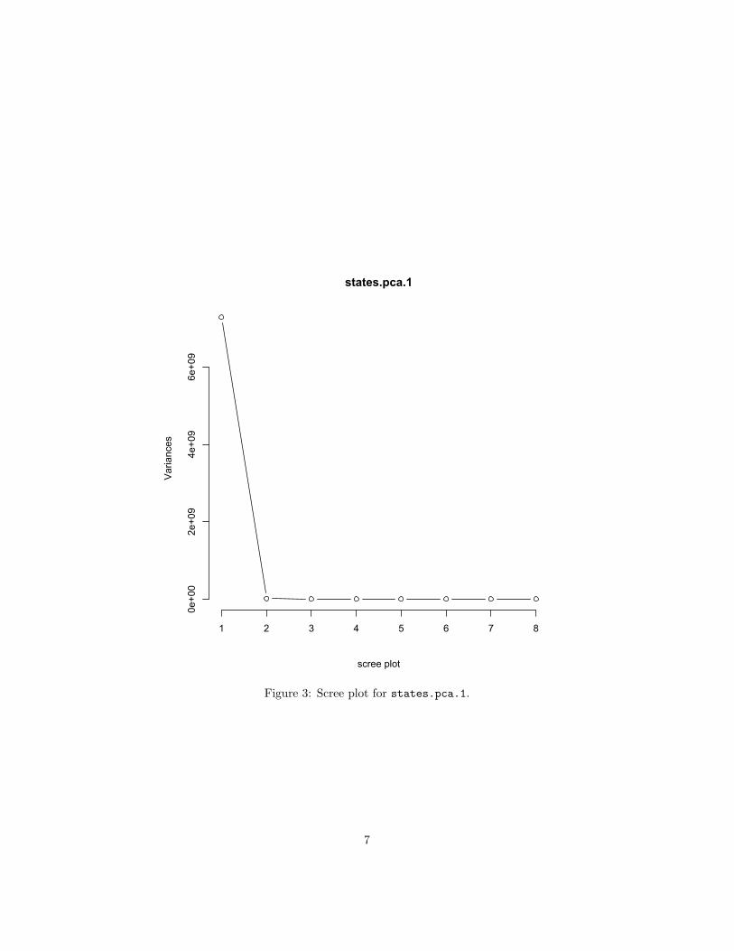
Figure 3: Scree plot for states.pca.1.

7

-0.2 0.0 0.2 0.4 0.6

-0.2

0.0

0.2

0.4

0.6

PC1

PC2

Alabama

Alaska

Arizona

Arkansas

California

Colorado

ConnecticutDelaware

Florida

GeorgiaHawaii

Idaho

Illinois

IndianaIowa

Kansas

Kentucky

Louisiana

Maine

Maryland

Massachusetts

Michigan

Minnesota

Mississippi

MissouriMontana

Nebraska

Nevada

New Hampshire

New Jersey

New Mexico

New York

North CarolinaNorth Dakota

Ohio

Oklahoma

OregonPennsylvania

Rhode Island

South CarolinaSouth Dakota

Tennessee

Texas

Utah

Vermont

VirginiaWashington

West Virginia

Wisconsin

Wyoming

-5 0 5 10 15

-50

510

15

PopulationIncome

IlliteracyLife Exp

MurderHS Grad

Frost

Area

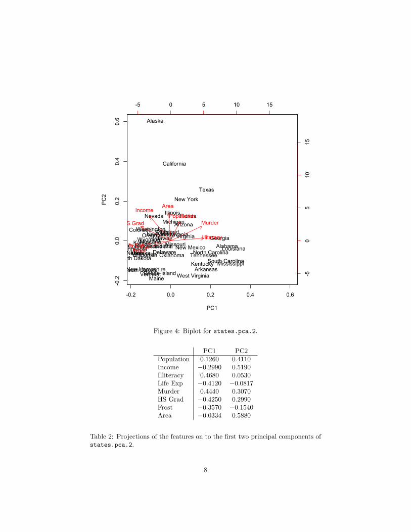
Figure 4: Biplot for states.pca.2.

PC1 PC2Population 0.1260 0.4110Income −0.2990 0.5190Illiteracy 0.4680 0.0530Life Exp −0.4120 −0.0817Murder 0.4440 0.3070HS Grad −0.4250 0.2990Frost −0.3570 −0.1540Area −0.0334 0.5880

Table 2: Projections of the features on to the first two principal components ofstates.pca.2.

8

-2 -1 0 1 2 3 4

-10

12

34

5

PC1

PC2

AL

AK

AZ

AR

CA

CO

CTDE

FL

GAHI

ID

IL

INIA

KS

KY

LA

ME

MD

MA

MI

MN

MS

MOMT

NE

NV

NH

NJ

NM

NY

NCND

OH

OK

OR PA

RI

SCSD

TN

TX

UT

VT

VAWA

WV

WI

WY

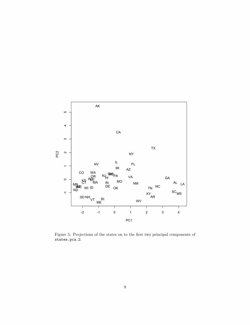
Figure 5: Projections of the states on to the first two principal components ofstates.pca.2.

9

states.pca.2

scree plot

Variances

0.0

0.5

1.0

1.5

2.0

2.5

3.0

3.5

1 2 3 4 5 6 7 8

Figure 6: Scree plot for states.pca.2.

10

-120 -110 -100 -90 -80 -70

3035

4045

50

longitude

latitude

AL

AK

AZAR

CA

CO

CT

DE

FL

GAHI

ID

IL IN

IA

KS

KY

LA

ME

MD

MA

MI

MN

MS

MO

MT

NE

NV

NH

NJ

NM

NY

NC

ND

OH

OK

OR

PARI

SC

SD

TN

TX

UT

VT

VA

WA

WV

WI

WY

Figure 7: States in their geographic locations, with name size being proportionalto the projection on to the first component of states.pca.2.

11

-120 -110 -100 -90 -80 -70

3035

4045

50

longitude

latitude

Alabama

Alaska

ArizonaArkansas

California

Colorado

Connecticut

Delaware

Florida

GeorgiaHawaii

Idaho

IllinoisIndiana

Iowa

KansasKentucky

Louisiana

Maine

Maryland

MassachusettsMichigan

Minnesota

Mississippi

Missouri

Montana

Nebraska

Nevada

New Hampshire

New Jersey

New Mexico

New York

North Carolina

North Dakota

Ohio

Oklahoma

Oregon

PennsylvaniaRhode Island

South Carolina

South Dakota

Tennessee

Texas

Utah

Vermont

Virginia

Washington

West Virginia

Wisconsin

Wyoming

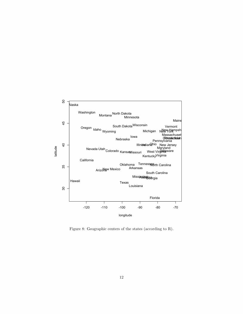
Figure 8: Geographic centers of the states (according to R).

12

(a) (3 pts) How does the command to create states.pca.1 differ fromthat creating states.pca.2? What do they do differently?

(b) (6 pts) Describe, in words, the first two principal components ofstates.pca.1

(c) (6 pts) Describe, in words, the first two principal components ofstates.pca.2

(d) (5 pts) Would you rather use states.pca.1 or states.pca.2 forfurther analysis? Pick one and explain your choice. (A choice withno or inadequate reasoning will get little or no credit.)

(e) (5 pts) Figure 7 shows the states in their geographic locations, withthe size of the label being proportional to the projection on to thefirst component (as per states.pca.2). What does this suggestabout the interpretation of that component?

(f) (5 pts extra credit) Figure 8 shows where R thinks the states arelocated (using states.centers). Does anything look odd about thefigure? Would you add these latitude and longitude values as fea-tures?

13

4. (25 points in all) In local linear embedding, we obtain an n×n matrix w,where wij is the weight on ~xj we use to reconstruct ~xi. Each row of wsums to one. We then try to find coordinates y1, y2, . . . yn which minimize

Φ(Y) =n∑

i=1

yi −n∑

j=1

wijyj

2

where Y is the n × 1 matrix of yi values (this is the q = 1 case, forsimplicity). In the notes, we showed that this is the same as minimizing

Φ(Y) = YT MY

whereM = ((I−w)T (I−w))

(a) (2 pts) Show that M is a symmetric matrix.

(b) (5 pts) Show that 1 is an eigenvector of M, and that its eigenvalueis zero.

(c) (3 pts) Show that Φ(Y) = Φ(Y + c1), where c is any constant and 1is the n× 1 matrix whose entries are all 1s. (Hint: one way is to usethe previous two parts.)

(d) (2 pts) Show that Φ(Y) is minimized by Y = 0.

(e) (3 pts) To avoid the trivial solution of setting all the yi to zero, we im-pose the constraint that n−1

∑ni=1 y2

i = 1. We use a Lagrange multi-plier to enforce this constraint; write down the Lagrangian (modifiedobjective function) for the constrained minimization problem.

(f) (10 pts) Show that a solution Y to the constrained minimizationproblem must be an eigenvector of M.

14