Principal Components Analysis - CMU Statisticscshalizi/uADA/12/lectures/ch18.pdf · Chapter 18...

Chapter 18

Principal Components Analysis

Principal components analysis (PCA) is one of a family of techniques for takinghigh-dimensional data, and using the dependencies between the variables to representit in a more tractable, lower-dimensional form, without losing too much information.PCA is one of the simplest and most robust ways of doing such dimensionalityreduction. It is also one of the oldest, and has been rediscovered many times inmany fields, so it is also known as the Karhunen-Loève transformation, the Hotellingtransformation, the method of empirical orthogonal functions, and singular valuedecomposition1. We will call it PCA.

18.1 Mathematics of Principal ComponentsWe start with p-dimensional vectors, and want to summarize them by projectingdown into a q -dimensional subspace. Our summary will be the projection of theoriginal vectors on to q directions, the principal components, which span the sub-space.

There are several equivalent ways of deriving the principal components mathe-matically. The simplest one is by finding the projections which maximize the vari-ance. The first principal component is the direction in space along which projectionshave the largest variance. The second principal component is the direction whichmaximizes variance among all directions orthogonal to the first. The k th componentis the variance-maximizing direction orthogonal to the previous k − 1 components.There are p principal components in all.

Rather than maximizing variance, it might sound more plausible to look for theprojection with the smallest average (mean-squared) distance between the originalvectors and their projections on to the principal components; this turns out to beequivalent to maximizing the variance.

Throughout, assume that the data have been “centered”, so that every variablehas mean 0. If we write the centered data in a matrix x, where rows are objects and

1Strictly speaking, singular value decomposition is a matrix algebra trick which is used in the mostcommon algorithm for PCA.

351

352 CHAPTER 18. PRINCIPAL COMPONENTS ANALYSIS

columns are variables, then xT x = nv, where v is the covariance matrix of the data.(You should check that last statement!)

18.1.1 Minimizing Projection ResidualsWe’ll start by looking for a one-dimensional projection. That is, we have p-dimensionalvectors, and we want to project them on to a line through the origin. We can specifythe line by a unit vector along it, �w, and then the projection of a data vector �xi on tothe line is �xi · �w, which is a scalar. (Sanity check: this gives us the right answer whenwe project on to one of the coordinate axes.) This is the distance of the projectionfrom the origin; the actual coordinate in p-dimensional space is (�xi · �w) �w. The meanof the projections will be zero, because the mean of the vectors �xi is zero:

1n

n�i=1(�xi · �w) �w =��

1n

n�i=1

xi

�· �w��w (18.1)

If we try to use our projected or image vectors instead of our original vectors,there will be some error, because (in general) the images do not coincide with theoriginal vectors. (When do they coincide?) The difference is the error or residual ofthe projection. How big is it? For any one vector, say �xi , it’s

��xi − ( �w · �xi ) �w�2 =��xi − ( �w · �xi ) �w� · ��xi − ( �w · �xi ) �w

�(18.2)

= �xi · �xi − �xi · ( �w · �xi ) �w (18.3)−( �w · �xi ) �w · �xi + ( �w · �xi ) �w · ( �w · �xi ) �w

= ��xi�2− 2( �w · �xi )2+ ( �w · �xi )

2 �w · �w (18.4)= �xi · �xi − ( �w · �xi )

2 (18.5)

since �w · �w = � �w�2 = 1. Add those residuals up across all the vectors:

M SE( �w) =1n

n�i=1��xi�2− ( �w · �xi )

2 (18.6)

=1n

�n�

i=1��xi�2−

n�i=1( �w · �xi )

2

�(18.7)

The first summation doesn’t depend on �w, so it doesn’t matter for trying to minimizethe mean squared residual. To make the MSE small, what we must do is make thesecond sum big, i.e., we want to maximize

1n

n�i=1( �w · �xi )

2 (18.8)

which we can see is the sample mean of ( �w · �xi )2. The mean of a square is always equal

to the square of the mean plus the variance:

1n

n�i=1( �w · �xi )

2 =

�1n

n�i=1

�xi · �w�2+Var��w · �xi�

(18.9)

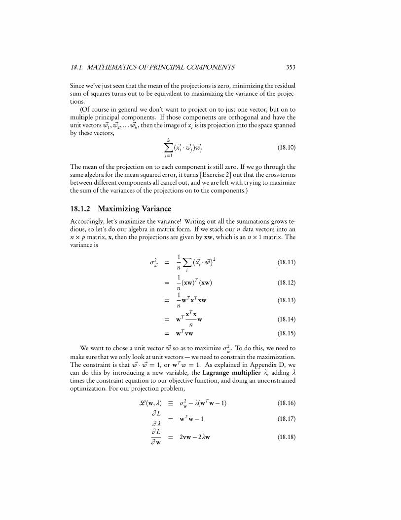
18.1. MATHEMATICS OF PRINCIPAL COMPONENTS 353

Since we’ve just seen that the mean of the projections is zero, minimizing the residualsum of squares turns out to be equivalent to maximizing the variance of the projec-tions.

(Of course in general we don’t want to project on to just one vector, but on tomultiple principal components. If those components are orthogonal and have theunit vectors �w1, �w2, . . . �wk , then the image of xi is its projection into the space spannedby these vectors,

k�j=1(�xi · �wj ) �wj (18.10)

The mean of the projection on to each component is still zero. If we go through thesame algebra for the mean squared error, it turns [Exercise 2] out that the cross-termsbetween different components all cancel out, and we are left with trying to maximizethe sum of the variances of the projections on to the components.)

18.1.2 Maximizing VarianceAccordingly, let’s maximize the variance! Writing out all the summations grows te-dious, so let’s do our algebra in matrix form. If we stack our n data vectors into ann× p matrix, x, then the projections are given by xw, which is an n× 1 matrix. Thevariance is

σ2�w =

1n

�i

��xi · �w�2 (18.11)

=1n(xw)T (xw) (18.12)

=1n

wT xT xw (18.13)

= wT xT xn

w (18.14)

= wT vw (18.15)

We want to chose a unit vector �w so as to maximize σ2�w . To do this, we need to

make sure that we only look at unit vectors — we need to constrain the maximization.The constraint is that �w · �w = 1, or wT w = 1. As explained in Appendix D, wecan do this by introducing a new variable, the Lagrange multiplier λ, adding λtimes the constraint equation to our objective function, and doing an unconstrainedoptimization. For our projection problem,

� (w,λ) ≡ σ2w−λ(wT w− 1) (18.16)

∂ L∂ λ

= wT w− 1 (18.17)

∂ L∂ w

= 2vw− 2λw (18.18)


Setting the derivatives to zero at the optimum, we get

wT w = 1 (18.19)vw = λw (18.20)

Thus, desired vector w is an eigenvector of the covariance matrix v, and the maxi-mizing vector will be the one associated with the largest eigenvalue λ. This is goodnews, because finding eigenvectors is something which can be done comparativelyrapidly, and because eigenvectors have many nice mathematical properties, which wecan use as follows.

We know that v is a p × p matrix, so it will have p different eigenvectors.2 Weknow that v is a covariance matrix, so it is symmetric, and then linear algebra tellsus that the eigenvectors must be orthogonal to one another. Again because v is acovariance matrix, it is a positive matrix, in the sense that �x · v�x ≥ 0 for any �x. Thistells us that the eigenvalues of v must all be ≥ 0.

The eigenvectors of v are the principal components of the data. We know thatthey are all orthogonal top each other from the previous paragraph, so together theyspan the whole p-dimensional space. The first principal component, i.e. the eigen-vector which goes the largest value of λ, is the direction along which the data havethe most variance. The second principal component, i.e. the second eigenvector, isthe direction orthogonal to the first component with the most variance. Because itis orthogonal to the first eigenvector, their projections will be uncorrelated. In fact,projections on to all the principal components are uncorrelated with each other. Ifwe use q principal components, our weight matrix w will be a p × q matrix, whereeach column will be a different eigenvector of the covariance matrix v. The eigen-values will give the total variance described by each component. The variance of theprojections on to the first q principal components is then

�qi=1 λi .

18.1.3 More Geometry; Back to the ResidualsSuppose that the data really are q -dimensional. Then v will have only q positiveeigenvalues, and p−q zero eigenvalues. If the data fall near a q -dimensional subspace,then p − q of the eigenvalues will be nearly zero.

If we pick the top q components, we can define a projection operator Pq . Theimages of the data are then xPq . The projection residuals are x− xPq or x(I−Pq ).(Notice that the residuals here are vectors, not just magnitudes.) If the data reallyare q -dimensional, then the residuals will be zero. If the data are approximately q -dimensional, then the residuals will be small. In any case, we can define the R2 of theprojection as the fraction of the original variance kept by the image vectors,

R2 ≡�q

i=1 λi�pj=1 λ j

(18.21)

just as the R2 of a linear regression is the fraction of the original variance of thedependent variable kept by the fitted values.

2Exception: if n < p, there are only n distinct eigenvectors and eigenvalues.

18.1. MATHEMATICS OF PRINCIPAL COMPONENTS 355

The q = 1 case is especially instructive. We know that the residual vectors are allorthogonal to the projections. Suppose we ask for the first principal component ofthe residuals. This will be the direction of largest variance which is perpendicular tothe first principal component. In other words, it will be the second principal com-ponent of the data. This suggests a recursive algorithm for finding all the principalcomponents: the k th principal component is the leading component of the residu-als after subtracting off the first k − 1 components. In practice, it is faster to useeigenvector-solvers to get all the components at once from v, but this idea is correctin principle.

This is a good place to remark that if the data really fall in a q -dimensional sub-space, then v will have only q positive eigenvalues, because after subtracting off thosecomponents there will be no residuals. The other p − q eigenvectors will all haveeigenvalue 0. If the data cluster around a q -dimensional subspace, then p − q of theeigenvalues will be very small, though how small they need to be before we can ne-glect them is a tricky question.3

Projections on to the first two or three principal components can be visualized;however they may not be enough to really give a good summary of the data. Usually,to get an R2 of 1, you need to use all p principal components.4 How many principalcomponents you should use depends on your data, and how big an R2 you need. Insome fields, you can get better than 80% of the variance described with just two orthree components. A sometimes-useful device is to plot 1−R2 versus the number ofcomponents, and keep extending the curve it until it flattens out.

18.1.4 Statistical Inference, or NotYou may have noticed, and even been troubled by, the fact that I have said nothingat all yet like “assume the data are drawn at random from some distribution”, or“assume the different rows of the data frame are statistically independent”. This isbecause no such assumption is required for principal components. All it does is say“these data can be summarized using projections along these directions”. It says noth-ing about the larger population or stochastic process the data came from; it doesn’teven suppose the latter exist.

However, we could add a statistical assumption and see how PCA behaves underthose conditions. The simplest one is to suppose that the data are IID draws froma distribution with covariance matrix V0. Then the sample covariance matrix V ≡1n XT X will converge on V0 as n →∞. Since the principal components are smoothfunctions of V (namely its eigenvectors), they will tend to converge as n grows5. So,

3Be careful when n < p. Any two points define a line, and three points define a plane, etc., so if thereare fewer data points than variables, it is necessarily true that the fall on a low-dimensional subspace. In§18.3.1, we represent stories in the New York Times as vectors with p ≈ 440, but n = 102. Finding thatonly 102 principal components keep all the variance is not an empirical discovery but a mathematicalartifact.

4The exceptions are when some of your variables are linear combinations of the others, so that youdon’t really have p different variables, or when n < p.

5There is a wrinkle if V0 has “degenerate” eigenvalues, i.e., two or more eigenvectors with the sameeigenvalue. Then any linear combination of those vectors is also an eigenvector, with the same eigenvalue(Exercise 3.) For instance, if V0 is the identity matrix, then every vector is an eigenvector, and PCA


Variable MeaningSports Binary indicator for being a sports carSUV Indicator for sports utility vehicleWagon IndicatorMinivan IndicatorPickup IndicatorAWD Indicator for all-wheel driveRWD Indicator for rear-wheel driveRetail Suggested retail price (US$)Dealer Price to dealer (US$)Engine Engine size (liters)Cylinders Number of engine cylindersHorsepower Engine horsepowerCityMPG City gas mileageHighwayMPG Highway gas mileageWeight Weight (pounds)Wheelbase Wheelbase (inches)Length Length (inches)Width Width (inches)

Table 18.1: Features for the 2004 cars data.

along with that additional assumption about the data-generating process, PCA doesmake a prediction: in the future, the principal components will look like they donow.

18.2 Example: CarsLet’s work an example. The data6 consists of 388 cars from the 2004 model year, with18 features. Eight features are binary indicators; the other 11 features are numerical(Table 18.1). All of the features except Type are numerical. Table 18.2 shows the firstfew lines from the data set. PCA only works with numerical variables, so we haveten of them to play with.

There are two R functions for doing PCA, princomp and prcomp, which differin how they do the actual calculation.7 The latter is generally more robust, so we’lljust use it.

cars04 = read.csv("cars-fixed04.dat")cars04.pca = prcomp(cars04[,8:18], scale.=TRUE)

routines will return an essentially arbitrary collection of mutually perpendicular vectors. Generically,however, any arbitrarily small tweak to V0 will break the degeneracy.

6On the course website; from http://www.amstat.org/publications/jse/datasets/04cars.txt, with incomplete records removed.

7princomp actually calculates the covariance matrix and takes its eigenvalues. prcomp uses a differenttechnique called “singular value decomposition”.

18.2. EXAMPLE: CARS 357

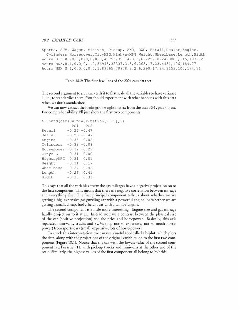
Sports, SUV, Wagon, Minivan, Pickup, AWD, RWD, Retail,Dealer,Engine,Cylinders,Horsepower,CityMPG,HighwayMPG,Weight,Wheelbase,Length,Width

Acura 3.5 RL,0,0,0,0,0,0,0,43755,39014,3.5,6,225,18,24,3880,115,197,72Acura MDX,0,1,0,0,0,1,0,36945,33337,3.5,6,265,17,23,4451,106,189,77Acura NSX S,1,0,0,0,0,0,1,89765,79978,3.2,6,290,17,24,3153,100,174,71

Table 18.2: The first few lines of the 2004 cars data set.

The second argument to prcomp tells it to first scale all the variables to have variance1, i.e., to standardize them. You should experiment with what happens with this datawhen we don’t standardize.

We can now extract the loadings or weight matrix from the cars04.pca object.For comprehensibility I’ll just show the first two components.

> round(cars04.pca$rotation[,1:2],2)PC1 PC2

Retail -0.26 -0.47Dealer -0.26 -0.47Engine -0.35 0.02Cylinders -0.33 -0.08Horsepower -0.32 -0.29CityMPG 0.31 0.00HighwayMPG 0.31 0.01Weight -0.34 0.17Wheelbase -0.27 0.42Length -0.26 0.41Width -0.30 0.31

This says that all the variables except the gas-mileages have a negative projection on tothe first component. This means that there is a negative correlation between mileageand everything else. The first principal component tells us about whether we aregetting a big, expensive gas-guzzling car with a powerful engine, or whether we aregetting a small, cheap, fuel-efficient car with a wimpy engine.

The second component is a little more interesting. Engine size and gas mileagehardly project on to it at all. Instead we have a contrast between the physical sizeof the car (positive projection) and the price and horsepower. Basically, this axisseparates mini-vans, trucks and SUVs (big, not so expensive, not so much horse-power) from sports-cars (small, expensive, lots of horse-power).

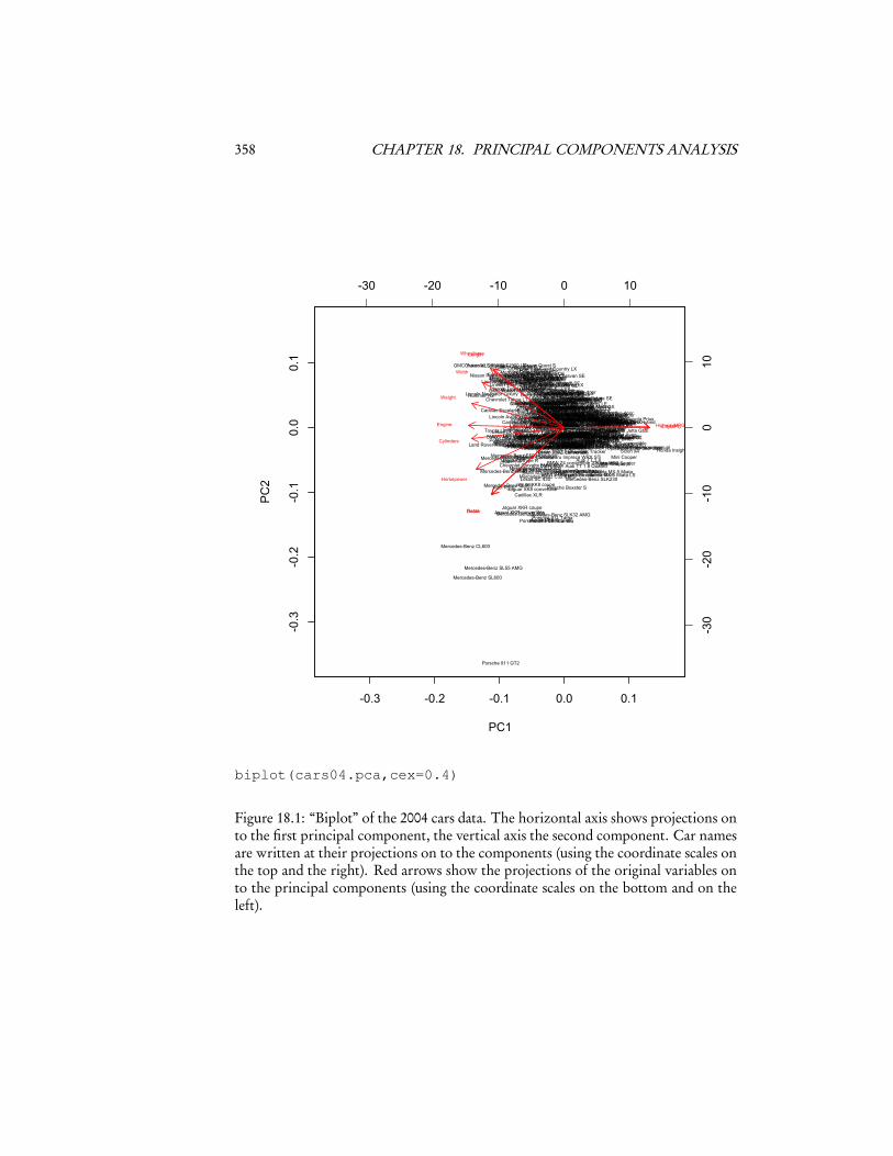
To check this interpretation, we can use a useful tool called a biplot, which plotsthe data, along with the projections of the original variables, on to the first two com-ponents (Figure 18.1). Notice that the car with the lowest value of the second com-ponent is a Porsche 911, with pick-up trucks and mini-vans at the other end of thescale. Similarly, the highest values of the first component all belong to hybrids.


-0.3 -0.2 -0.1 0.0 0.1

-0.3

-0.2

-0.1

0.0

0.1

PC1

PC2

Acura 3.5 RLAcura 3.5 RL NavigationAcura MDX

Acura NSX S

Acura RSX

Acura TL Acura TSXAudi A4 1.8TAudi A4 1.8T convertible

Audi A4 3.0 convertible

Audi A4 3.0Audi A4 3.0 Quattro manualAudi A4 3.0 Quattro autoAudi A4 3.0 Quattro convertible

Audi A6 2.7 Turbo Quattro four-door

Audi A6 3.0Audi A6 3.0 Avant QuattroAudi A6 3.0 Quattro

Audi A6 4.2 Quattro

Audi A8 L Quattro

Audi S4 Avant QuattroAudi S4 Quattro

Audi RS 6

Audi TT 1.8Audi TT 1.8 Quattro

Audi TT 3.2

BMW 325iBMW 325CiBMW 325Ci convertible

BMW 325xiBMW 325xi Sport

BMW 330CiBMW 330Ci convertible

BMW 330iBMW 330xi

BMW 525i four-door

BMW 530i four-door

BMW 545iA four-doorBMW 745i four-doorBMW 745Li four-door

BMW M3BMW M3 convertible

BMW X3 3.0i

BMW X5 4.4i

BMW Z4 convertible 2.5i two-door

BMW Z4 convertible 3.0i two-door

Buick Century CustomBuick LeSabre Custom four-door

Buick LeSabre LimitedBuick Park Avenue

Buick Park Avenue Ultra

Buick RainierBuick Regal GSBuick Regal LSBuick Rendezvous CX

Cadillac CTS VVTCadillac Deville

Cadillac Deville DTS

Cadillac Escaladet

Cadillac SevilleCadillac SRX V8

Cadillac XLR

Chevrolet Aveo

Chevrolet Astro

Chevrolet Aveo LS

Chevrolet Cavalier two-doorChevrolet Cavalier four-doorChevrolet Cavalier LS

Chevrolet Corvette

Chevrolet Corvette convertible

Chevrolet ImpalaChevrolet Impala LS

Chevrolet Impala SSChevrolet Malibu

Chevrolet Malibu LSChevrolet Malibu LT

Chevrolet Malibu Maxx

Chevrolet Monte Carlo LSChevrolet Monte Carlo SS

Chevrolet Suburban 1500 LT

Chevrolet Tahoe LT

Chevrolet Tracker

Chevrolet TrailBlazer LTChevrolet Venture LS

Chrysler 300MChrysler 300M Special Edition

Chrysler Concorde LXChrysler Concorde LXi

Chrysler Crossfire

Chrysler Pacifica

Chrysler PT Cruiser

Chrysler PT Cruiser GT

Chrysler PT Cruiser Limited

Chrysler Sebring

Chrysler Sebring Touring

Chrysler Sebring convertibleChrysler Sebring Limited convertible

Chrysler Town and Country LX

Chrysler Town and Country LimitedDodge Caravan SE

Dodge Durango SLTDodge Grand Caravan SXT

Dodge Intrepid ESDodge Intrepid SE

Dodge Neon SEDodge Neon SXT

Dodge Stratus SXTDodge Stratus SE

Ford Crown VictoriaFord Crown Victoria LX

Ford Crown Victoria LX Sport

Ford Escape XLS

Ford Expedition 4.6 XLT

Ford Explorer XLT V6

Ford Focus LXFord Focus SE

Ford Focus SVT

Ford Focus ZTWFord Focus ZX5Ford Focus ZX3

Ford Freestar SE

Ford Mustang

Ford Mustang GT Premium

Ford Taurus LXFord Taurus SEFord Taurus SES Duratec

Ford Thunderbird Deluxe

GMC Envoy XUV SLE

GMC Safari SLEGMC Yukon 1500 SLE

GMC Yukon XL 2500 SLT

Honda Accord EX

Honda Accord EX V6

Honda Accord LXHonda Accord LX V6

Honda Civic EXHonda Civic DXHonda Civic HXHonda Civic LX

Honda Civic Si

Honda Civic HybridHonda CR-V LXHonda Element LX

Honda Insight

Honda Odyssey EXHonda Odyssey LX

Honda Pilot LX

Honda S2000

Hummer H2

Hyundai AccentHyundai Accent GLHyundai Accent GT

Hyundai Elantra GLSHyundai Elantra GTHyundai Elantra GT hatchHyundai Santa Fe GLS

Hyundai Sonata GLSHyundai Sonata LX

Hyundai Tiburon GT V6

Hyundai XG350Hyundai XG350 LInfiniti FX35

Infiniti FX45Infiniti G35Infiniti G35 Sport CoupeInfiniti G35 AWDInfiniti I35

Infiniti M45Infiniti Q45 Luxury

Isuzu Ascender S

Isuzu Rodeo SJaguar S-Type 3.0

Jaguar S-Type 4.2

Jaguar S-Type R

Jaguar Vanden Plas

Jaguar X-Type 2.5Jaguar X-Type 3.0Jaguar XJ8

Jaguar XJR

Jaguar XK8 coupeJaguar XK8 convertible

Jaguar XKR coupeJaguar XKR convertible

Jeep Grand Cherokee Laredo

Jeep Liberty Sport

Jeep Wrangler Sahara

Kia Optima LX

Kia Optima LX V6

Kia Rio autoKia Rio manualKia Rio Cinco

Kia Sedona LX

Kia Sorento LX

Kia SpectraKia Spectra GSKia Spectra GSX

Land Rover Discovery SELand Rover Freelander SE

Land Rover Range Rover HSE

Lexus ES 330Lexus GS 300

Lexus GS 430

Lexus GX 470

Lexus IS 300 manualLexus IS 300 autoLexus IS 300 SportCrossLexus LS 430

Lexus LX 470

Lexus SC 430

Lexus RX 330

Lincoln Aviator Ultimate

Lincoln LS V6 LuxuryLincoln LS V6 Premium

Lincoln LS V8 SportLincoln LS V8 Ultimate

Lincoln Navigator Luxury

Lincoln Town Car SignatureLincoln Town Car Ultimate

Lincoln Town Car Ultimate L

Mazda6 iMazda MPV ES

Mazda MX-5 MiataMazda MX-5 Miata LS

Mazda Tribute DX 2.0

Mercedes-Benz C32 AMG

Mercedes-Benz C230 Sport

Mercedes-Benz C240Mercedes-Benz C240 RWDMercedes-Benz C240 AWD

Mercedes-Benz C320

Mercedes-Benz C320 Sport two-door

Mercedes-Benz C320 Sport four-door

Mercedes-Benz CL500

Mercedes-Benz CL600

Mercedes-Benz CLK320

Mercedes-Benz CLK500

Mercedes-Benz E320Mercedes-Benz E320 four-door

Mercedes-Benz E500Mercedes-Benz E500 four-door

Mercedes-Benz G500

Mercedes-Benz ML500Mercedes-Benz S430

Mercedes-Benz S500

Mercedes-Benz SL500

Mercedes-Benz SL55 AMG

Mercedes-Benz SL600

Mercedes-Benz SLK230

Mercedes-Benz SLK32 AMG

Mercury Grand Marquis GSMercury Grand Marquis LS PremiumMercury Grand Marquis LS Ultimate

Mercury Marauder

Mercury Monterey Luxury

Mercury Mountaineer

Mercury Sable GSMercury Sable GS four-doorMercury Sable LS Premium

Mini CooperMini Cooper S

Mitsubishi Diamante LS

Mitsubishi Eclipse GTSMitsubishi Eclipse Spyder GT

Mitsubishi EndeavorMitsubishi Galant

Mitsubishi Lancer Evolution

Mitsubishi Montero

Mitsubishi Outlander

Nissan 350ZNissan 350Z Enthusiast

Nissan Altima S

Nissan Altima SENissan Maxima SENissan Maxima SLNissan Murano

Nissan Pathfinder SE

Nissan Pathfinder Armada SE

Nissan Quest S

Nissan Quest SE

Nissan Sentra 1.8Nissan Sentra 1.8 SNissan Sentra SE-R

Nissan Xterra XEOldsmobile Alero GLS

Oldsmobile Alero GX

Oldsmobile Silhouette GL

Pontiac Aztekt

Porsche Cayenne S

Pontiac Grand Am GT

Pontiac Grand Prix GT1Pontiac Grand Prix GT2

Pontiac Montana

Pontiac Montana EWB

Pontiac Sunfire 1SAPontiac Sunfire 1SCPontiac Vibe

Porsche 911 CarreraPorsche 911 Carrera 4SPorsche 911 Targa

Porsche 911 GT2

Porsche Boxster

Porsche Boxster S

Saab 9-3 Arc

Saab 9-3 Arc SportSaab 9-3 Aero

Saab 9-3 Aero convertible

Saab 9-5 Arc

Saab 9-5 AeroSaab 9-5 Aero four-door

Saturn Ion1Saturn Ion2Saturn Ion2 quad coupeSaturn Ion3Saturn Ion3 quad coupe

Saturn L300Saturn L300-2

Saturn VUE

Scion xAScion xB

Subaru ForesterSubaru Impreza 2.5 RS

Subaru Impreza WRX

Subaru Impreza WRX STi

Subaru Legacy GTSubaru Legacy LSubaru Outback

Subaru Outback Limited Sedan

Subaru Outback H6Subaru Outback H-6 VDCSuzuki Aeno SSuzuki Aerio LXSuzuki Aerio SX

Suzuki Forenza SSuzuki Forenza EX

Suzuki Verona LX

Suzuki Vitara LX

Suzuki XL-7 EXToyota 4Runner SR5 V6

Toyota Avalon XLToyota Avalon XLS

Toyota Camry LE

Toyota Camry LE V6Toyota Camry XLE V6

Toyota Camry Solara SE

Toyota Camry Solara SE V6Toyota Camry Solara SLE V6 two-door

Toyota Celica

Toyota Corolla CEToyota Corolla SToyota Corolla LE

Toyota Echo two-door manualToyota Echo two-door autoToyota Echo four-door

Toyota Highlander V6

Toyota Land Cruiser

Toyota Matrix

Toyota MR2 Spyder

Toyota Prius

Toyota RAV4

Toyota Sequoia SR5Toyota Sienna CE

Toyota Sienna XLE

Volkswagen GolfVolkswagen GTI

Volkswagen Jetta GL

Volkswagen Jetta GLI

Volkswagen Jetta GLS

Volkswagen New Beetle GLS 1.8TVolkswagen New Beetle GLS convertible

Volkswagen Passat GLSVolkswagen Passat GLS four-door

Volkswagen Passat GLX V6 4MOTION four-door

Volkswagen Passat W8Volkswagen Passat W8 4MOTION

Volkswagen Touareg V6

Volvo C70 LPTVolvo C70 HPT

Volvo S40

Volvo S60 2.5

Volvo S60 T5

Volvo S60 R

Volvo S80 2.5TVolvo S80 2.9

Volvo S80 T6 Volvo V40

Volvo XC70Volvo XC90 T6

-30 -20 -10 0 10

-30

-20

-10

010

RetailDealer

Engine

Cylinders

Horsepower

CityMPGHighwayMPG

Weight

WheelbaseLength

Width

biplot(cars04.pca,cex=0.4)

Figure 18.1: “Biplot” of the 2004 cars data. The horizontal axis shows projections onto the first principal component, the vertical axis the second component. Car namesare written at their projections on to the components (using the coordinate scales onthe top and the right). Red arrows show the projections of the original variables onto the principal components (using the coordinate scales on the bottom and on theleft).

18.3. LATENT SEMANTIC ANALYSIS 359

18.3 Latent Semantic AnalysisInformation retrieval systems (like search engines) and people doing computationaltext analysis often represent documents as what are called bags of words: documentsare represented as vectors, where each component counts how many times each wordin the dictionary appears in the text. This throws away information about word or-der, but gives us something we can work with mathematically. Part of the represen-tation of one document might look like:

a abandoned abc ability able about above abroad absorbed absorbing abstract43 0 0 0 0 10 0 0 0 0 1

and so on through to “zebra”, “zoology”, “zygote”, etc. to the end of the dictionary.These vectors are very, very large! At least in English and similar languages, thesebag-of-word vectors have three outstanding properties:

1. Most words do not appear in most documents; the bag-of-words vectors arevery sparse (most entries are zero).

2. A small number of words appear many times in almost all documents; thesewords tell us almost nothing about what the document is about. (Examples:“the”, “is”, “of”, “for”, “at”, “a”, “and”, “here”, “was”, etc.)

3. Apart from those hyper-common words, most words’ counts are correlatedwith some but not all other words; words tend to come in bunches whichappear together.

Taken together, this suggests that we do not really get a lot of value from keepingaround all the words. We would be better off if we could project down a smallernumber of new variables, which we can think of as combinations of words that tendto appear together in the documents, or not at all. But this tendency needn’t be abso-lute — it can be partial because the words mean slightly different things, or becauseof stylistic differences, etc. This is exactly what principal components analysis does.

To see how this can be useful, imagine we have a collection of documents (a cor-pus), which we want to search for documents about agriculture. It’s entirely possiblethat many documents on this topic don’t actually contain the word “agriculture”, justclosely related words like “farming”. A simple search on “agriculture” will miss them.But it’s very likely that the occurrence of these related words is well-correlated withthe occurrence of “agriculture”. This means that all these words will have similar pro-jections on to the principal components, and will be easy to find documents whoseprincipal components projection is like that for a query about agriculture. This iscalled latent semantic indexing.

To see why this is indexing, think about what goes into coming up with an indexfor a book by hand. Someone draws up a list of topics and then goes through thebook noting all the passages which refer to the topic, and maybe a little bit of whatthey say there. For example, here’s the start of the entry for “Agriculture” in theindex to Adam Smith’s The Wealth of Nations:


AGRICULTURE, the labour of, does not admit of such subdivisionsas manufactures, 6; this impossibility of separation, prevents agricul-ture from improving equally with manufactures, 6; natural state of, ina new colony, 92; requires more knowledge and experience than mostmechanical professions, and yet is carried on without any restrictions,127; the terms of rent, how adjusted between landlord and tenant, 144;is extended by good roads and navigable canals, 147; under what circum-stances pasture land is more valuable than arable, 149; gardening not avery gainful employment, 152–3; vines the most profitable article of cul-ture, 154; estimates of profit from projects, very fallacious, ib.; cattle andtillage mutually improve each other, 220; . . .

and so on. (Agriculture is an important topic in The Wealth of Nations.) It’s askinga lot to hope for a computer to be able to do something like this, but we could atleast hope for a list of pages like “6,92,126,144,147,152 − −3,154,220, . . .”. Onecould imagine doing this by treating each page as its own document, forming itsbag-of-words vector, and then returning the list of pages with a non-zero entry for“agriculture”. This will fail: only two of those nine pages actually contains thatword, and this is pretty typical. On the other hand, they are full of words stronglycorrelated with “agriculture”, so asking for the pages which are most similar in theirprincipal components projection to that word will work great.8

At first glance, and maybe even second, this seems like a wonderful trick forextracting meaning, or semantics, from pure correlations. Of course there are also allsorts of ways it can fail, not least from spurious correlations. If our training corpushappens to contain lots of documents which mention “farming” and “Kansas”, aswell as “farming” and “agriculture”, latent semantic indexing will not make a bigdistinction between the relationship between “agriculture” and “farming” (which isgenuinely semantic) and that between “Kansas” and “farming” (which is accidental,and probably wouldn’t show up in, say, a corpus collected from Europe).

Despite this susceptibility to spurious correlations, latent semantic indexing is anextremely useful technique in practice, and the foundational papers (Deerwester et al.,1990; Landauer and Dumais, 1997) are worth reading.

18.3.1 Principal Components of the New York Times

To get a more concrete sense of how latent semantic analysis works, and how it re-veals semantic information, let’s apply it to some data. The accompanying R file andR workspace contains some news stories taken from the New York Times AnnotatedCorpus (Sandhaus, 2008), which consists of about 1.8 million stories from the Times,from 1987 to 2007, which have been hand-annotated by actual human beings withstandardized machine-readable information about their contents. From this corpus,I have randomly selected 57 stories about art and 45 stories about music, and turnedthem into a bag-of-words data frame, one row per story, one column per word; plusan indicator in the first column of whether the story is one about art or one about

8Or it should anyway; I haven’t actually done the experiment with this book.

18.3. LATENT SEMANTIC ANALYSIS 361

music.9 The original data frame thus has 102 rows, and 4432 columns: the categoricallabel, and 4431 columns with counts for every distinct word that appears in at leastone of the stories.10

The PCA is done as it would be for any other data:

nyt.pca <- prcomp(nyt.frame[,-1])nyt.latent.sem <- nyt.pca$rotation

We need to omit the first column in the first command because it contains categor-ical variables, and PCA doesn’t apply to them. The second command just picksout the matrix of projections of the variables on to the components — this is calledrotation because it can be thought of as rotating the coordinate axes in feature-vector space.

Now that we’ve done this, let’s look at what the leading components are.

> signif(sort(nyt.latent.sem[,1],decreasing=TRUE)[1:30],2)music trio theater orchestra composers opera0.110 0.084 0.083 0.067 0.059 0.058

theaters m festival east program y0.055 0.054 0.051 0.049 0.048 0.048

jersey players committee sunday june concert0.047 0.047 0.046 0.045 0.045 0.045

symphony organ matinee misstated instruments p0.044 0.044 0.043 0.042 0.041 0.041

X.d april samuel jazz pianist society0.041 0.040 0.040 0.039 0.038 0.038

> signif(sort(nyt.latent.sem[,1],decreasing=FALSE)[1:30],2)she her ms i said mother cooper

-0.260 -0.240 -0.200 -0.150 -0.130 -0.110 -0.100my painting process paintings im he mrs

-0.094 -0.088 -0.071 -0.070 -0.068 -0.065 -0.065me gagosian was picasso image sculpture baby

-0.063 -0.062 -0.058 -0.057 -0.056 -0.056 -0.055artists work photos you nature studio out-0.055 -0.054 -0.051 -0.051 -0.050 -0.050 -0.050says like

-0.050 -0.049

These are the thirty words with the largest positive and negative projections on to thefirst component.11 The words with positive projections are mostly associated with

9Actually, following standard practice in language processing, I’ve normalized the bag-of-word vectorsso that documents of different lengths are comparable, and used “inverse document-frequency weighting”to de-emphasize hyper-common words like “the” and emphasize more informative words. See the lecturenotes for data mining if you’re interested.

10If we were trying to work with the complete corpus, we should expect at least 50000 words, andperhaps more.

11Which direction is positive and which negative is of course arbitrary; basically it depends on internalchoices in the algorithm.


music, those with negative components with the visual arts. The letters “m” and “p”show up with msuic because of the combination “p.m”, which our parsing breaksinto two single-letter words, and because stories about music give show-times moreoften than do stories about art. Personal pronouns appear with art stories becausemore of those quote people, such as artists or collectors.12

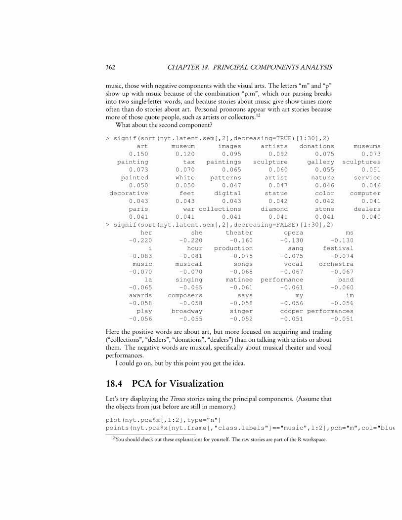
What about the second component?

> signif(sort(nyt.latent.sem[,2],decreasing=TRUE)[1:30],2)art museum images artists donations museums

0.150 0.120 0.095 0.092 0.075 0.073painting tax paintings sculpture gallery sculptures

0.073 0.070 0.065 0.060 0.055 0.051painted white patterns artist nature service

0.050 0.050 0.047 0.047 0.046 0.046decorative feet digital statue color computer

0.043 0.043 0.043 0.042 0.042 0.041paris war collections diamond stone dealers0.041 0.041 0.041 0.041 0.041 0.040

> signif(sort(nyt.latent.sem[,2],decreasing=FALSE)[1:30],2)her she theater opera ms

-0.220 -0.220 -0.160 -0.130 -0.130i hour production sang festival

-0.083 -0.081 -0.075 -0.075 -0.074music musical songs vocal orchestra-0.070 -0.070 -0.068 -0.067 -0.067

la singing matinee performance band-0.065 -0.065 -0.061 -0.061 -0.060awards composers says my im-0.058 -0.058 -0.058 -0.056 -0.056play broadway singer cooper performances

-0.056 -0.055 -0.052 -0.051 -0.051

Here the positive words are about art, but more focused on acquiring and trading(“collections”, “dealers”, “donations”, “dealers”) than on talking with artists or aboutthem. The negative words are musical, specifically about musical theater and vocalperformances.

I could go on, but by this point you get the idea.

18.4 PCA for VisualizationLet’s try displaying the Times stories using the principal components. (Assume thatthe objects from just before are still in memory.)

plot(nyt.pca$x[,1:2],type="n")points(nyt.pca$x[nyt.frame[,"class.labels"]=="music",1:2],pch="m",col="blue")

12You should check out these explanations for yourself. The raw stories are part of the R workspace.

18.4. PCA FOR VISUALIZATION 363

-0.4 -0.3 -0.2 -0.1 0.0 0.1 0.2

-0.3

-0.2

-0.1

0.0

0.1

0.2

PC1

PC2

mm

m

m

mm

m

mm

m

m

m

m

m

m

m

m

m

m

m

m mm

m

m

m

m

m

m

m

m

m

m

mm

m

m

m

m

m

mm

m

mm

a

a

a

a

a

a

a

a

a

a

aaa

a

a

aa

a a

a

aa

a

a

aaa

a

a a

aa

a

a

a

a

aa

a

a

a

a

aa

a

aa

a

aa

a

a

a

a

a

a

a

Figure 18.2: Projection of the Times stories on to the first two principal components.Labels: “a” for art stories, “m” for music.

points(nyt.pca$x[nyt.frame[,"class.labels"]=="art",1:2],pch="a",col="red")

The first command makes an empty plot — I do this just to set up the axes nicelyfor the data which will actually be displayed. The second and third commands plot ablue “m” at the location of each music story, and a red “a” at the location of each artstory. The result is Figure 18.2.

Notice that even though we have gone from 4431 dimensions to 2, and so thrownaway a lot of information, we could draw a line across this plot and have most ofthe art stories on one side of it and all the music stories on the other. If we letourselves use the first four or five principal components, we’d still have a thousand-fold savings in dimensions, but we’d be able to get almost-perfect separation betweenthe two classes. This is a sign that PCA is really doing a good job at summarizing theinformation in the word-count vectors, and in turn that the bags of words give us a


lot of information about the meaning of the stories.The figure also illustrates the idea of multidimensional scaling, which means

finding low-dimensional points to represent high-dimensional data by preserving thedistances between the points. If we write the original vectors as �x1,�x2, . . .�xn , and theirimages as �y1,�y2, . . .�yn , then the MDS problem is to pick the images to minimize thedifference in distances:

�i

�j �=i

��yi −�yj�−��xi −�xj�

�2(18.22)

This will be small if distances between the image points are all close to the distancesbetween the original points. PCA accomplishes this precisely because �yi is itself closeto �xi (on average).

18.5 PCA CautionsTrying to guess at what the components might mean is a good idea, but like many godideas it’s easy to go overboard. Specifically, once you attach an idea in your mind toa component, and especially once you attach a name to it, it’s very easy to forget thatthose are names and ideas you made up; to reify them, as you might reify clusters.Sometimes the components actually do measure real variables, but sometimes theyjust reflect patterns of covariance which have many different causes. If I did a PCAof the same variables but for, say, European cars, I might well get a similar first com-ponent, but the second component would probably be rather different, since SUVsare much less common there than here.

A more important example comes from population genetics. Starting in the late1960s, L. L. Cavalli-Sforza and collaborators began a huge project of mapping hu-man genetic variation — of determining the frequencies of different genes in differentpopulations throughout the world. (Cavalli-Sforza et al. (1994) is the main summary;Cavalli-Sforza has also written several excellent popularizations.) For each point inspace, there are a very large number of variables, which are the frequencies of the var-ious genes among the people living there. Plotted over space, this gives a map of thatgene’s frequency. What they noticed (unsurprisingly) is that many genes had simi-lar, but not identical, maps. This led them to use PCA, reducing the huge numberof variables (genes) to a few components. Results look like Figure 18.3. They inter-preted these components, very reasonably, as signs of large population movements.The first principal component for Europe and the Near East, for example, was sup-posed to show the expansion of agriculture out of the Fertile Crescent. The third,centered in steppes just north of the Caucasus, was supposed to reflect the expansionof Indo-European speakers towards the end of the Bronze Age. Similar stories weretold of other components elsewhere.

Unfortunately, as Novembre and Stephens (2008) showed, spatial patterns likethis are what one should expect to get when doing PCA of any kind of spatial datawith local correlations, because that essentially amounts to taking a Fourier trans-form, and picking out the low-frequency components.13 They simulated genetic dif-

13Remember that PCA re-writes the original vectors as a weighted sum of new, orthogonal vectors, just

18.6. EXERCISES 365

fusion processes, without any migration or population expansion, and got results thatlooked very like the real maps (Figure 18.4). This doesn’t mean that the stories of themaps must be wrong, but it does undercut the principal components as evidence forthose stories.

18.6 Exercises1. Step through the pca.R file on the class website. Then replicate the analysis

of the cars data given above.

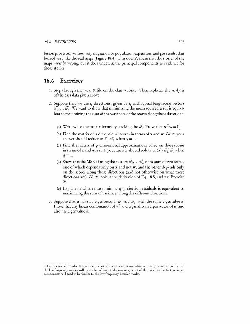
2. Suppose that we use q directions, given by q orthogonal length-one vectors�w1, . . . �wq . We want to show that minimizing the mean squared error is equiva-lent to maximizing the sum of the variances of the scores along these directions.

(a) Write w for the matrix forms by stacking the �wi . Prove that wT w= Iq .

(b) Find the matrix of q -dimensional scores in terms of x and w. Hint: youranswer should reduce to �xi · �w1 when q = 1.

(c) Find the matrix of p-dimensional approximations based on these scoresin terms of x and w. Hint: your answer should reduce to (�xi · �w1) �w1 whenq = 1.

(d) Show that the MSE of using the vectors �w1, . . . �wq is the sum of two terms,one of which depends only on x and not w, and the other depends onlyon the scores along those directions (and not otherwise on what thosedirections are). Hint: look at the derivation of Eq. 18.5, and use Exercise2a.

(e) Explain in what sense minimizing projection residuals is equivalent tomaximizing the sum of variances along the different directions.

3. Suppose that u has two eigenvectors, �w1 and �w2, with the same eigenvalue a.Prove that any linear combination of �w1 and �w2 is also an eigenvector of u, andalso has eigenvalue a.

as Fourier transforms do. When there is a lot of spatial correlation, values at nearby points are similar, sothe low-frequency modes will have a lot of amplitude, i.e., carry a lot of the variance. So first principalcomponents will tend to be similar to the low-frequency Fourier modes.


Figure 18.3: Principal components of genetic variation in the old world, according toCavalli-Sforza et al. (1994), as re-drawn by Novembre and Stephens (2008).

18.6. EXERCISES 367

Figure 18.4: How the PCA patterns can arise as numerical artifacts (far left column)or through simple genetic diffusion (next column). From Novembre and Stephens(2008).

Principal Components Analysis - CMU Statisticscshalizi/uADA/12/lectures/ch18.pdf · Chapter 18...

Documents

Transcript of Principal Components Analysis - CMU Statisticscshalizi/uADA/12/lectures/ch18.pdf · Chapter 18...