Time-Series Analysis and Forecasting – Part V To read at home.
32
Time-Series Analysis and Forecasting – Part V To read at home
-
Upload
laura-ward -
Category
Documents
-
view
218 -
download
1
Transcript of Time-Series Analysis and Forecasting – Part V To read at home.
Time-Series Analysis and Forecasting – Part V
To read at home
Analytical smoothing of time series (continued)
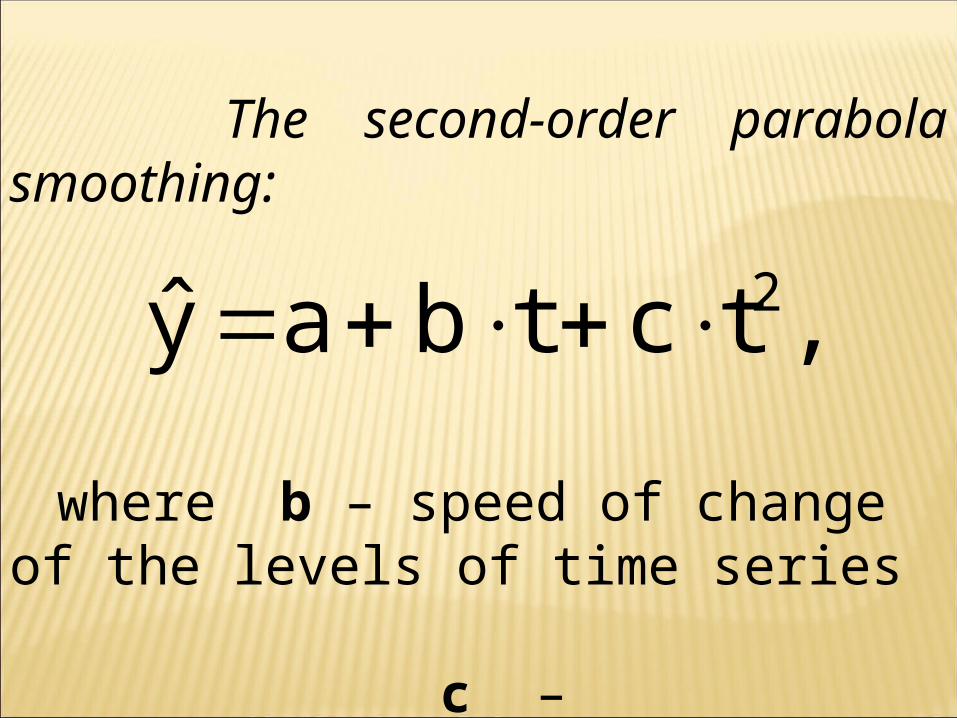
The second-order parabola smoothing:
where b – speed of change of the levels of time series
c – acceleration
2y a b t c t ,
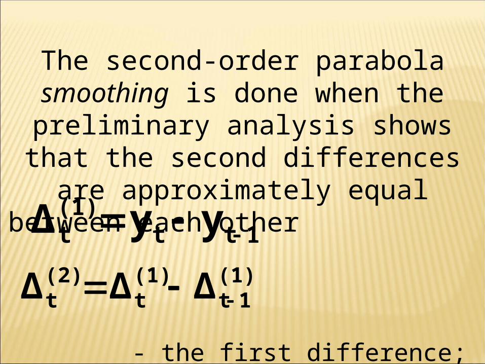
The second-order parabola smoothing is done when the preliminary analysis shows
that the second differences are approximately equal between each other
- the first difference;
- the second difference
1tt(1)t yyΔ
(1)1t
(1)t
(2)t ΔΔΔ
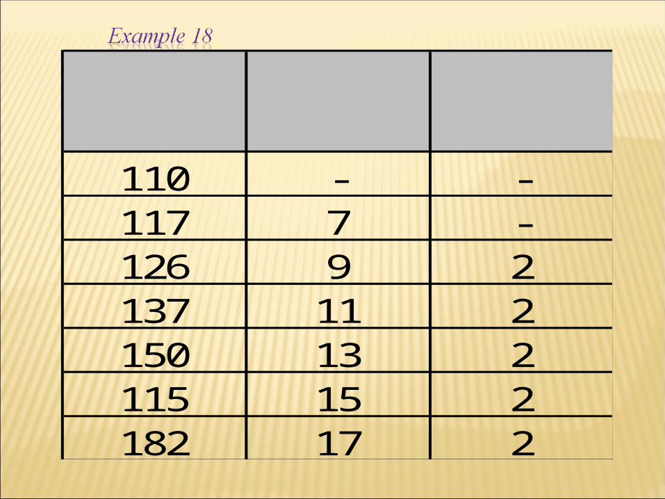
110 - -117 7 -126 9 2137 11 2150 13 2115 15 2182 17 2
ty (1)tΔ
(2)tΔ
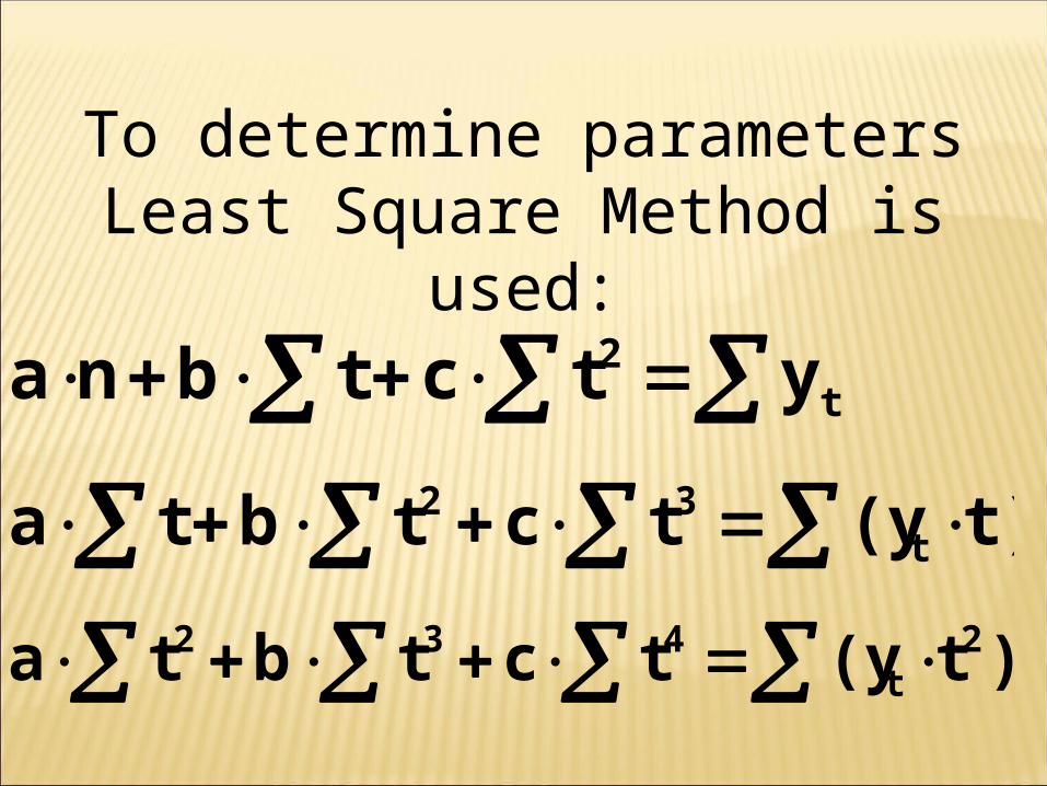
To determine parameters Least Square Method is used:
t2 ytctbna
t)(ytctbta t32
)t(ytctbta 2t
432
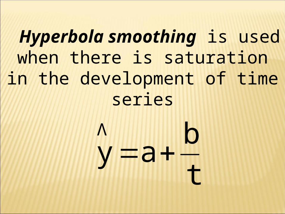
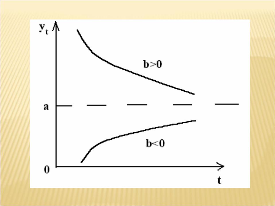
Hyperbola smoothing is used when there is saturation in the development
of time series
t
bay
Λ
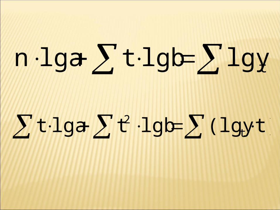
tlgylgbtlgan
t)(lgylgbtlgat t2
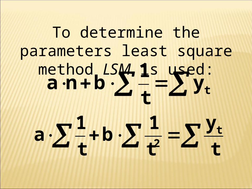
To determine the parameters least square method LSM is used:
tyt
1bna
t
y
t
1b
t
1a t
2
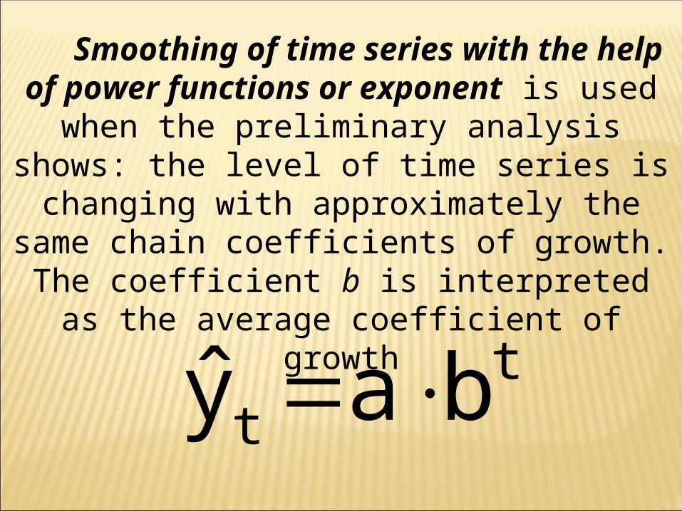
Smoothing of time series with the help of power functions or exponent is used when the
preliminary analysis shows: the level of time series is changing with approximately the same chain
coefficients of growth. The coefficient b is interpreted as the average coefficient of growth
tty a b
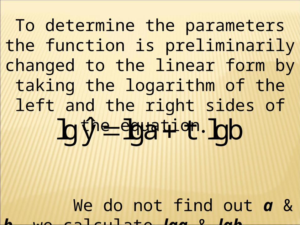
To determine the parameters the function is preliminarily changed to the linear form by taking the logarithm of the left and the right
sides of the equation
We do not find out a & b, we calculate lga & lgb
ˆlg y lga t lgb
Statistics for Business and Economics, 6e © 2007 Pearson Education, Inc. Chap 19-13
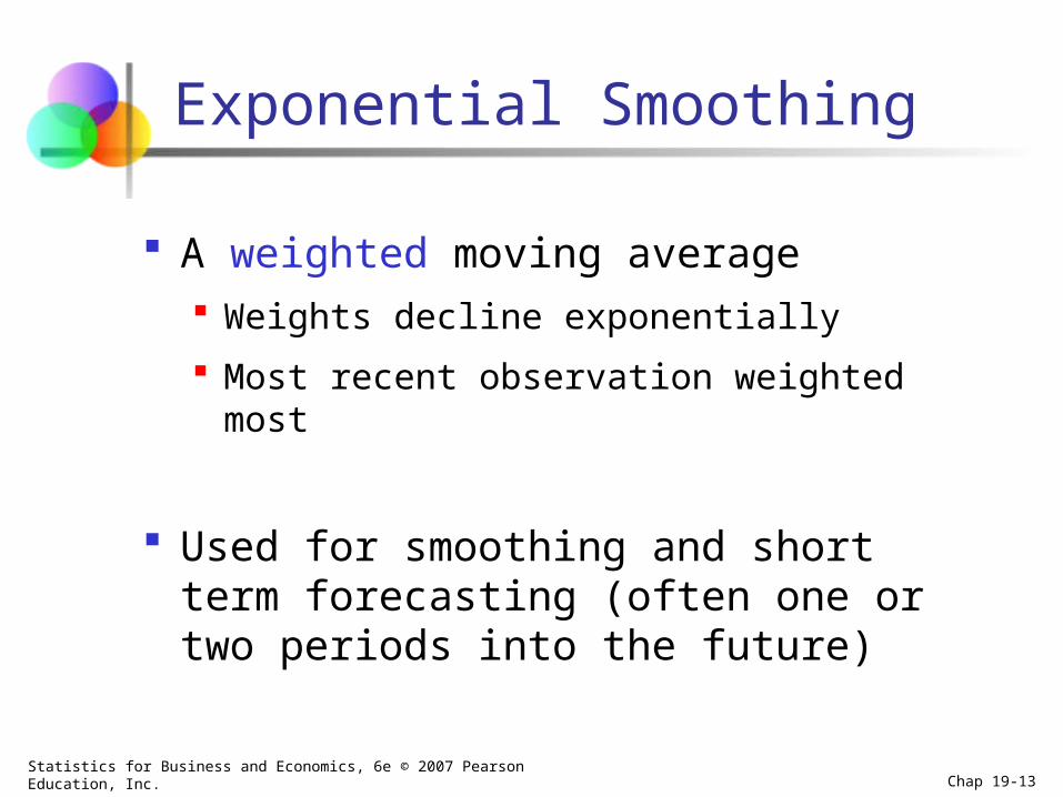
Exponential Smoothing
A weighted moving average Weights decline exponentially
Most recent observation weighted most
Used for smoothing and short term forecasting (often one or two periods into the future)
Statistics for Business and Economics, 6e © 2007 Pearson Education, Inc. Chap 19-14
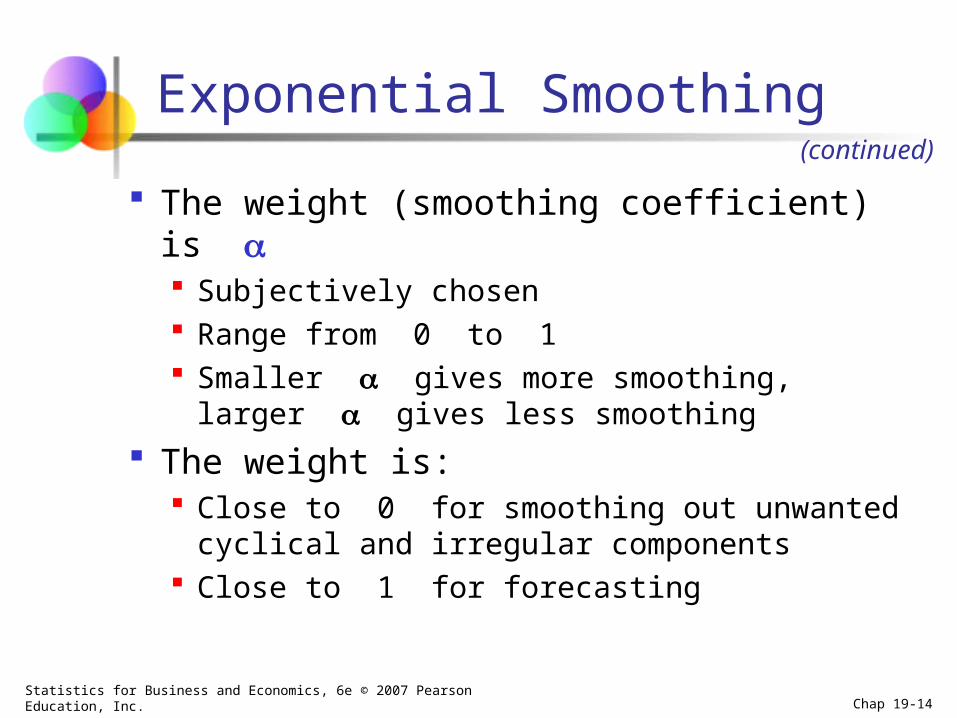
Exponential Smoothing
The weight (smoothing coefficient) is Subjectively chosen Range from 0 to 1 Smaller gives more smoothing, larger
gives less smoothing
The weight is: Close to 0 for smoothing out unwanted cyclical
and irregular components Close to 1 for forecasting
(continued)
Statistics for Business and Economics, 6e © 2007 Pearson Education, Inc. Chap 19-15
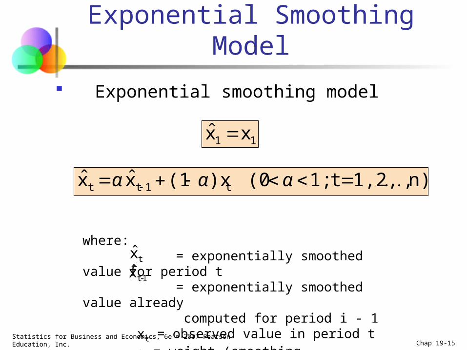
Exponential Smoothing Model
Exponential smoothing model
where: = exponentially smoothed value for period t = exponentially smoothed value already
computed for period i - 1 xt = observed value in period t = weight (smoothing coefficient), 0 < < 1
11 xx ˆ
n),1,2,t1;(0)x(1xx t1tt ααα ˆˆ
tx
1-tx
Statistics for Business and Economics, 6e © 2007 Pearson Education, Inc. Chap 19-16
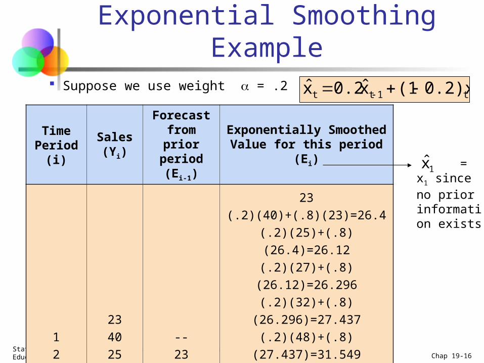
Exponential Smoothing Example Suppose we use weight = .2
Time Period
(i)
Sales(Yi)
Forecast from prior
period (Ei-1)
Exponentially Smoothed Value for this period (Ei)
1
2
3
4
5
6
7
8
9
10
etc.
23
40
25
27
32
48
33
37
37
50
etc.
--
23
26.4
26.12
26.296
27.437
31.549
31.840
32.872
33.697
etc.
23
(.2)(40)+(.8)(23)=26.4
(.2)(25)+(.8)(26.4)=26.12
(.2)(27)+(.8)(26.12)=26.296
(.2)(32)+(.8)(26.296)=27.437
(.2)(48)+(.8)(27.437)=31.549
(.2)(48)+(.8)(31.549)=31.840
(.2)(33)+(.8)(31.840)=32.872
(.2)(37)+(.8)(32.872)=33.697
(.2)(50)+(.8)(33.697)=36.958
etc.
= x1 since no prior information exists
1x
t1tt 0.2)x(1x0.2x ˆˆ
Statistics for Business and Economics, 6e © 2007 Pearson Education, Inc. Chap 19-17
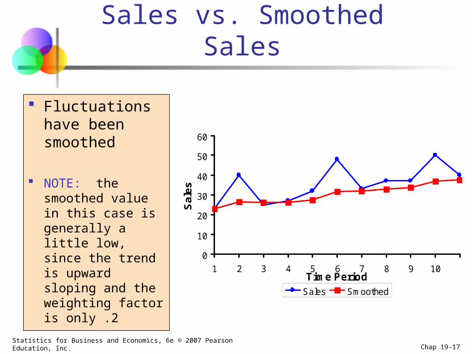
Sales vs. Smoothed Sales
Fluctuations have been smoothed
NOTE: the smoothed value in this case is generally a little low, since the trend is upward sloping and the weighting factor is only .2
0
10
20
30
40
50
60
1 2 3 4 5 6 7 8 9 10Time Period
Sa
les
Sales Smoothed
Statistics for Business and Economics, 6e © 2007 Pearson Education, Inc. Chap 19-18
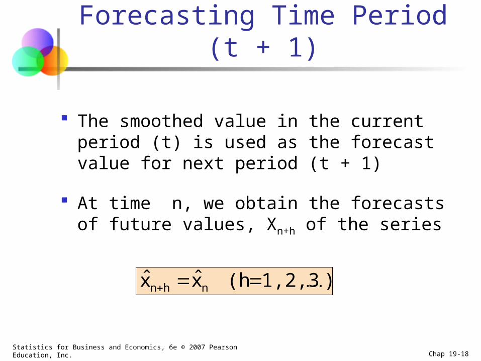
Forecasting Time Period (t + 1)
The smoothed value in the current period (t) is used as the forecast value for next period (t + 1)
At time n, we obtain the forecasts of future values, Xn+h of the series
)1,2,3(hxx nhn ˆˆ
Statistics for Business and Economics, 6e © 2007 Pearson Education, Inc. Chap 19-19
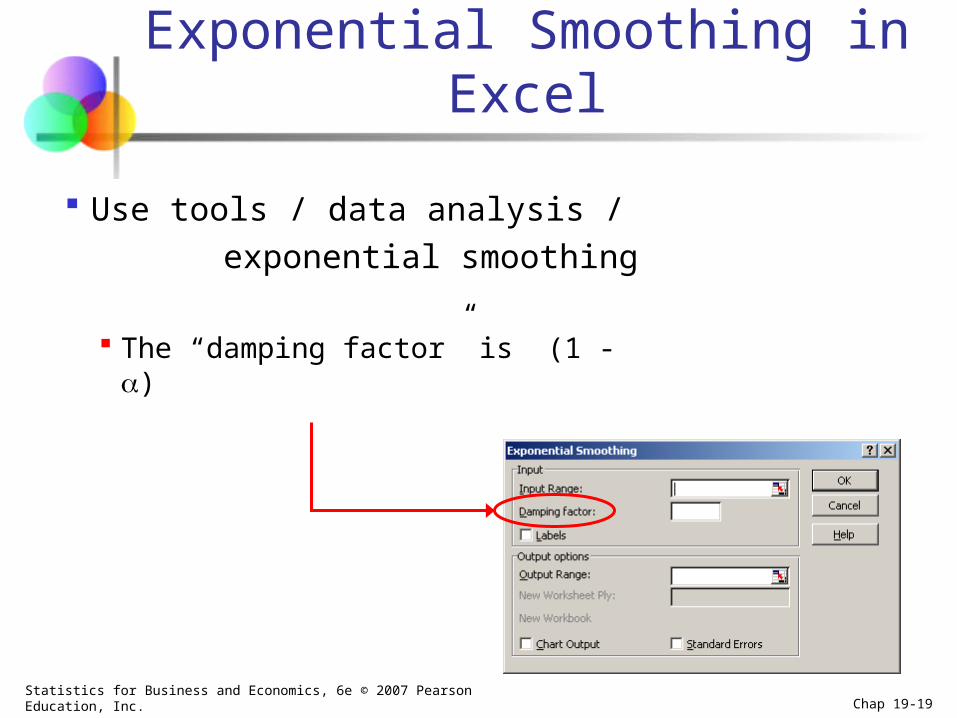
Exponential Smoothing in Excel
Use tools / data analysis /
exponential smoothing
The “damping factor” is (1 - )
Statistics for Business and Economics, 6e © 2007 Pearson Education, Inc. Chap 19-20
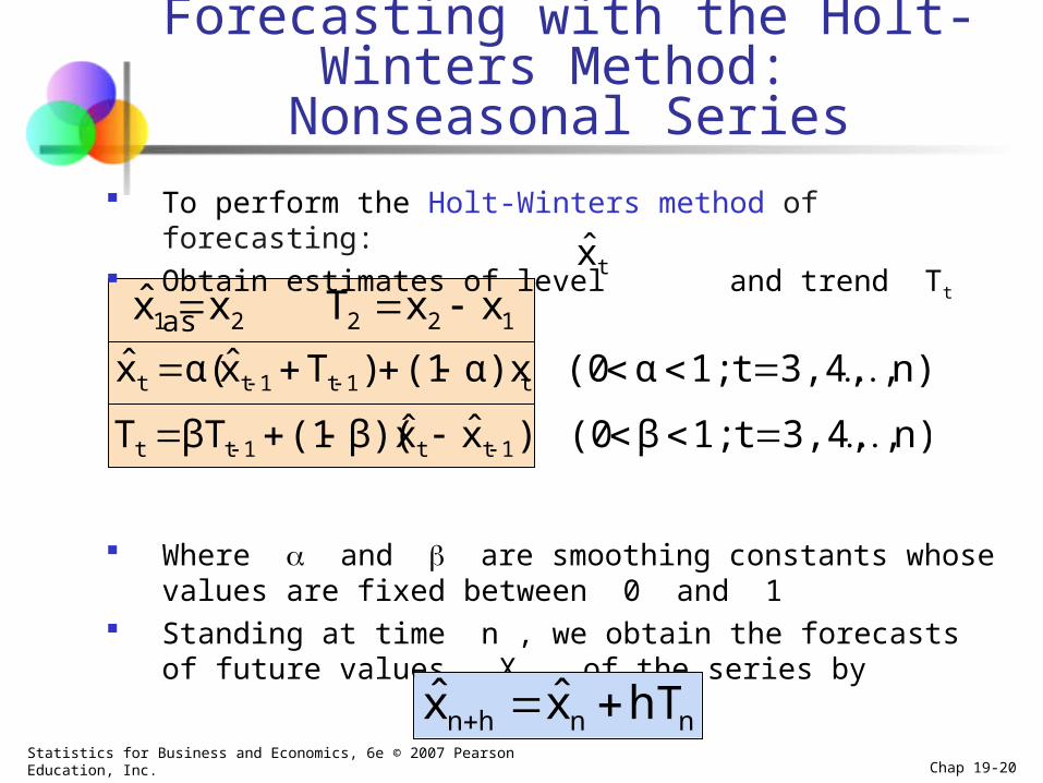
To perform the Holt-Winters method of forecasting: Obtain estimates of level and trend Tt as
Where and are smoothing constants whose values are fixed between 0 and 1
Standing at time n , we obtain the forecasts of future values, Xn+h of the series by
Forecasting with the Holt-Winters Method: Nonseasonal Series
tx
12221 xxTxx ˆ
n),3,4,t1;α(0α)x(1)Txα(x t1t1tt ˆˆ
nnhn hTxx ˆˆ
n),3,4,t1;β(0)xxβ)((1βTT 1tt1tt ˆˆ
Statistics for Business and Economics, 6e © 2007 Pearson Education, Inc. Chap 19-21
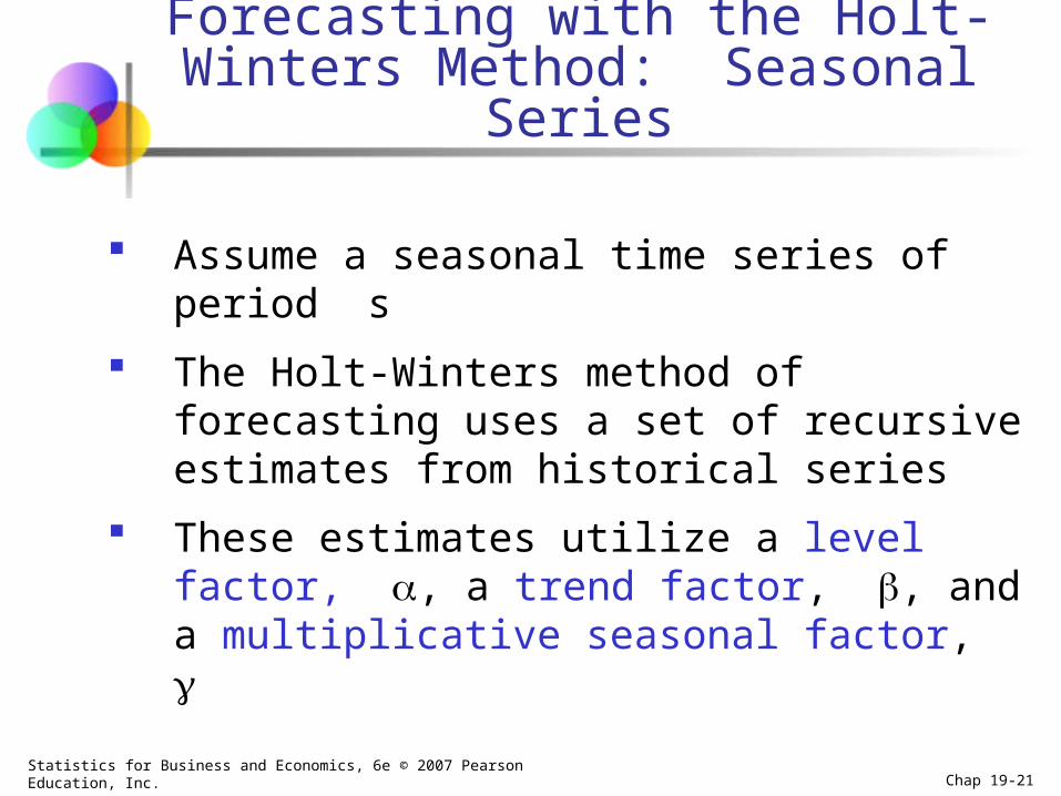
Assume a seasonal time series of period s
The Holt-Winters method of forecasting uses a set of recursive estimates from historical series
These estimates utilize a level factor, , a trend factor, , and a multiplicative seasonal factor,
Forecasting with the Holt-Winters Method: Seasonal Series
Statistics for Business and Economics, 6e © 2007 Pearson Education, Inc. Chap 19-22
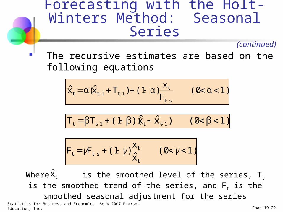
The recursive estimates are based on the following equations
Forecasting with the Holt-Winters Method: Seasonal Series
1)α(0F
xα)(1)Txα(x
st
t1t1tt
ˆˆ
1)(0x
x)(1FF
t
tstt γγγ
ˆ
1)β(0)xxβ)((1βTT 1tt1tt ˆˆ
Where is the smoothed level of the series, Tt is the smoothed trend of the series, and Ft is the smoothed seasonal adjustment for the series
tx
(continued)
Statistics for Business and Economics, 6e © 2007 Pearson Education, Inc. Chap 19-23
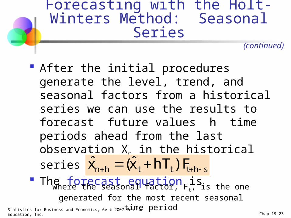
After the initial procedures generate the level, trend, and seasonal factors from a historical series we can use the results to forecast future values h time periods ahead from the last observation Xn in the historical series
The forecast equation is
shttthn )FhTx(x ˆˆ
where the seasonal factor, Ft, is the one generated for the most recent seasonal time period
Forecasting with the Holt-Winters Method: Seasonal Series
(continued)
Statistics for Business and Economics, 6e © 2007 Pearson Education, Inc. Chap 19-24
Autoregressive Models
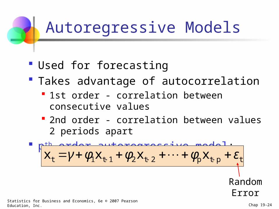
Used for forecasting Takes advantage of autocorrelation
1st order - correlation between consecutive values 2nd order - correlation between values 2 periods
apart
pth order autoregressive model:
Random Error
tptp2t21t1t xxxx εφφφγ
Statistics for Business and Economics, 6e © 2007 Pearson Education, Inc. Chap 19-25
Autoregressive Models
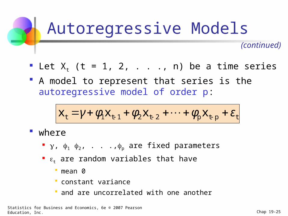
Let Xt (t = 1, 2, . . ., n) be a time series
A model to represent that series is the autoregressive model of order p:
where , 1 2, . . .,p are fixed parameters
t are random variables that have
mean 0
constant variance
and are uncorrelated with one another
tptp2t21t1t xxxx εφφφγ
(continued)
Statistics for Business and Economics, 6e © 2007 Pearson Education, Inc. Chap 19-26
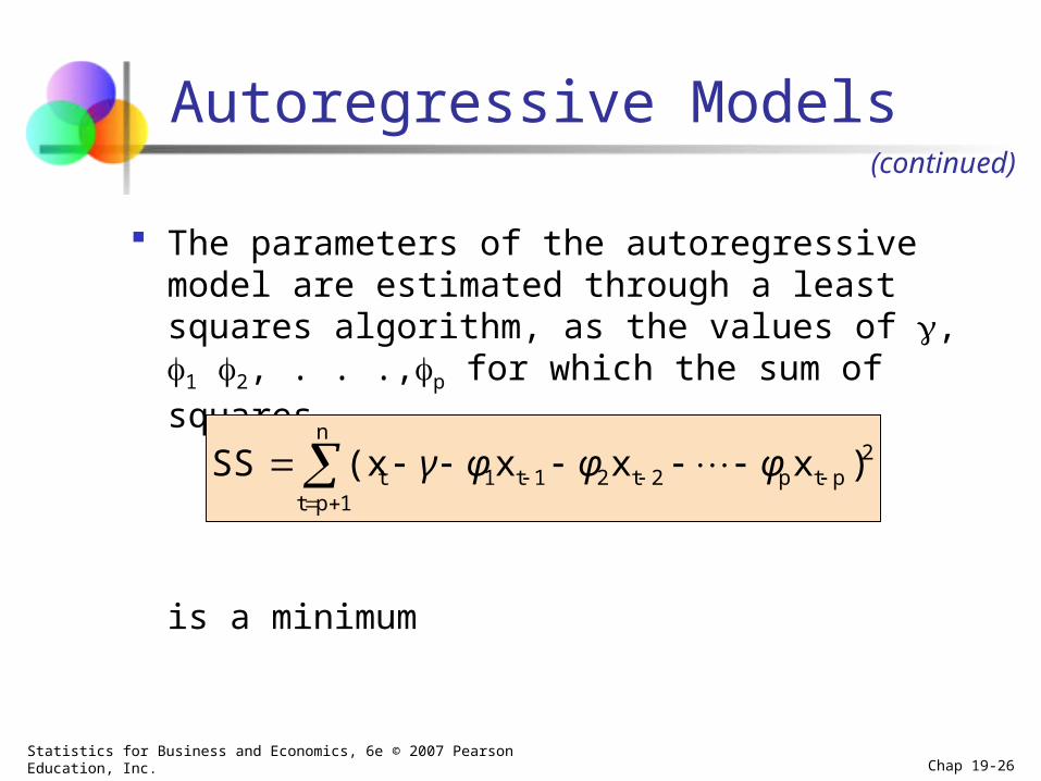
Autoregressive Models
The parameters of the autoregressive model are estimated through a least squares algorithm, as the values of , 1 2, . . .,p for which the sum of squares
is a minimum
2ptp2t21t1
n
1ptt )xxx(xSS
φφφγ
(continued)
Statistics for Business and Economics, 6e © 2007 Pearson Education, Inc. Chap 19-27
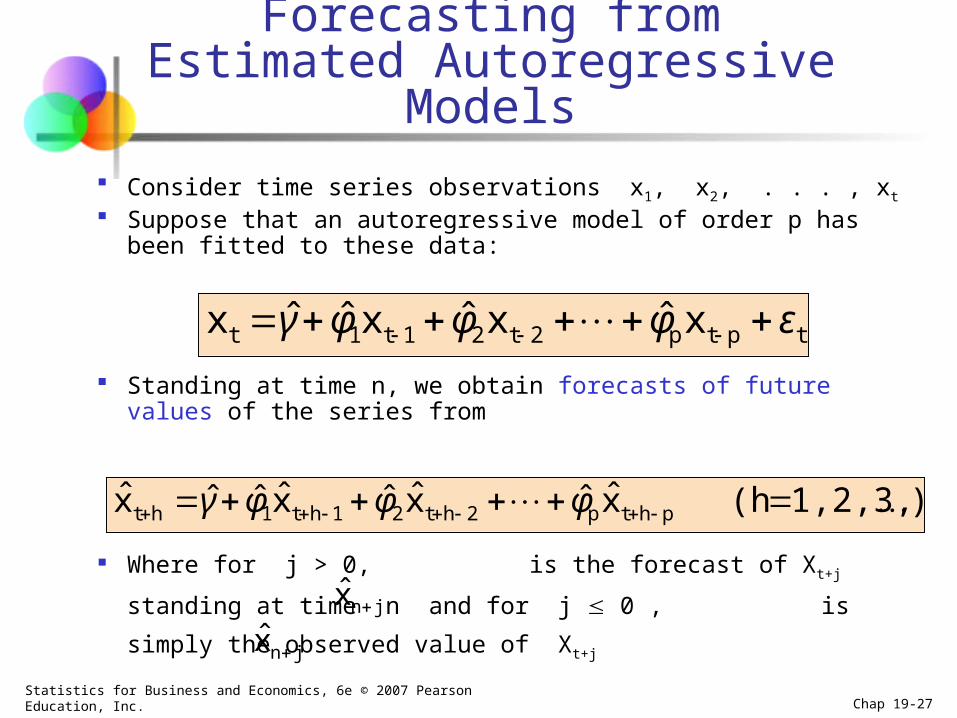
Forecasting from Estimated Autoregressive Models
Consider time series observations x1, x2, . . . , xt Suppose that an autoregressive model of order p has been fitted to
these data:
Standing at time n, we obtain forecasts of future values of the series from
Where for j > 0, is the forecast of Xt+j standing at time n and
for j 0 , is simply the observed value of Xt+j
tptp2t21t1t xxxx εφφφγ ˆˆˆˆ
)1,2,3,(hxxxx phtp2ht21ht1ht ˆˆˆˆˆˆˆˆ φφφγ
jnx ˆ
jnx ˆ
Statistics for Business and Economics, 6e © 2007 Pearson Education, Inc. Chap 19-28
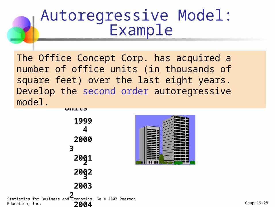
Autoregressive Model: Example
Year Units
1999 4 2000 3 2001 2 2002 3 2003 2 2004 2 2005 4 2006 6
The Office Concept Corp. has acquired a number of office units (in thousands of square feet) over the last eight years. Develop the second order autoregressive model.
Statistics for Business and Economics, 6e © 2007 Pearson Education, Inc. Chap 19-29
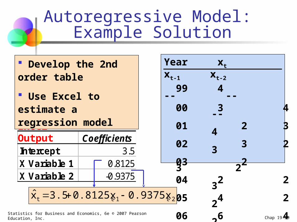
Autoregressive Model: Example Solution
Year xt xt-1 xt-2
99 4 -- -- 00 3 4 -- 01 2 3 4 02 3 2 3 03 2 3 2 04 2 2 3 05 4 2 2 06 6 4 2
CoefficientsIntercept 3.5X Variable 1 0.8125X Variable 2 -0.9375
Excel Output
Develop the 2nd order table
Use Excel to estimate a regression model
2t1tt 0.9375x0.8125x3.5x ˆ
Statistics for Business and Economics, 6e © 2007 Pearson Education, Inc. Chap 19-30
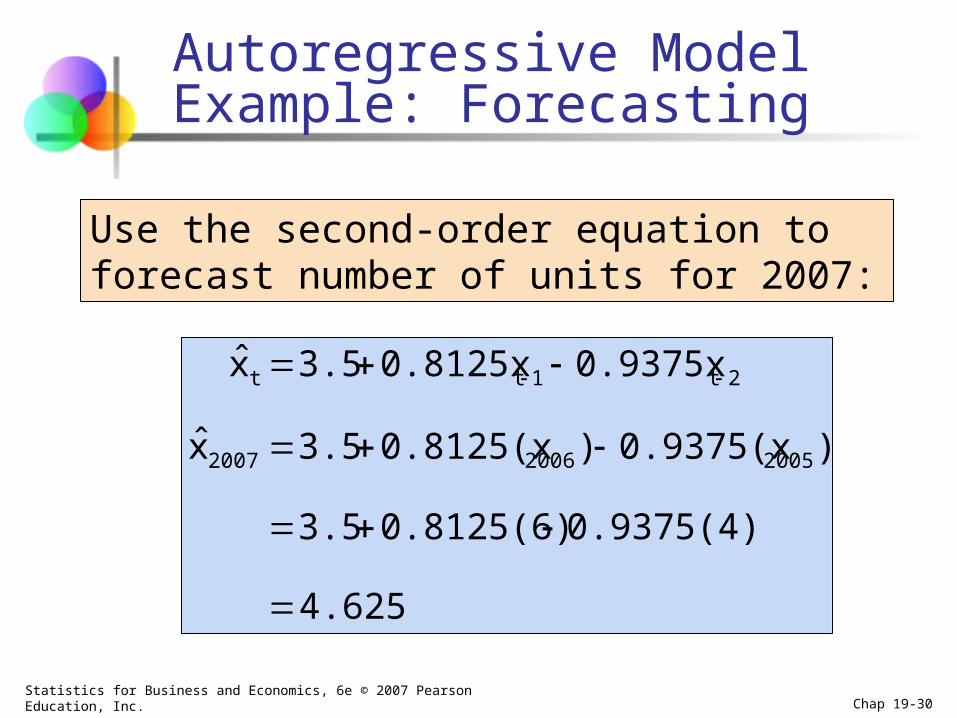
Autoregressive Model Example: Forecasting
Use the second-order equation to forecast number of units for 2007:
4.625
0.9375(4)0.8125(6)3.5
)0.9375(x)0.8125(x3.5x
0.9375x0.8125x3.5x
200520062007
2t1tt
ˆ
ˆ
Statistics for Business and Economics, 6e © 2007 Pearson Education, Inc. Chap 19-31
Autoregressive Modeling Steps
Choose p
Form a series of “lagged predictor” variables xt-1 , xt-2 , … ,xt-p
Run a regression model using all p variables
Test model for significance
Use model for forecasting

Merci beaucoup!