Automatic Time Series Forecasting: The forecast Package · PDF fileAutomatic Time Series...
22
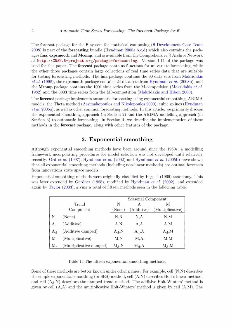
JSS Journal of Statistical Software July 2008, Volume 27, Issue 3. http://www.jstatsoft.org/ Automatic Time Series Forecasting: The forecast Package for R Rob J. Hyndman Monash University Yeasmin Khandakar Monash University Abstract Automatic forecasts of large numbers of univariate time series are often needed in business and other contexts. We describe two automatic forecasting algorithms that have been implemented in the forecast package for R. The first is based on innovations state space models that underly exponential smoothing methods. The second is a step-wise algorithm for forecasting with ARIMA models. The algorithms are applicable to both seasonal and non-seasonal data, and are compared and illustrated using four real time series. We also briefly describe some of the other functionality available in the forecast package. Keywords : ARIMA models, automatic forecasting, exponential smoothing, prediction inter- vals, state space models, time series, R. 1. Introduction Automatic forecasts of large numbers of univariate time series are often needed in business. It is common to have over one thousand product lines that need forecasting at least monthly. Even when a smaller number of forecasts are required, there may be nobody suitably trained in the use of time series models to produce them. In these circumstances, an automatic forecasting algorithm is an essential tool. Automatic forecasting algorithms must determine an appropriate time series model, estimate the parameters and compute the forecasts. They must be robust to unusual time series patterns, and applicable to large numbers of series without user intervention. The most popular automatic forecasting algorithms are based on either exponential smoothing or ARIMA models. In this article, we discuss the implementation of two automatic univariate forecasting methods in the forecast package for R. We also briefly describe some univariate forecasting methods that are part of the forecast package.
Transcript of Automatic Time Series Forecasting: The forecast Package · PDF fileAutomatic Time Series...
JSS Journal of Statistical SoftwareJuly 2008, Volume 27, Issue 3. http://www.jstatsoft.org/
Automatic Time Series Forecasting: The forecast
Package for R
Rob J. HyndmanMonash University
Yeasmin KhandakarMonash University
Abstract
Automatic forecasts of large numbers of univariate time series are often needed inbusiness and other contexts. We describe two automatic forecasting algorithms that havebeen implemented in the forecast package for R. The first is based on innovations statespace models that underly exponential smoothing methods. The second is a step-wisealgorithm for forecasting with ARIMA models. The algorithms are applicable to bothseasonal and non-seasonal data, and are compared and illustrated using four real timeseries. We also briefly describe some of the other functionality available in the forecastpackage.
Keywords: ARIMA models, automatic forecasting, exponential smoothing, prediction inter-vals, state space models, time series, R.
1. Introduction
Automatic forecasts of large numbers of univariate time series are often needed in business.It is common to have over one thousand product lines that need forecasting at least monthly.Even when a smaller number of forecasts are required, there may be nobody suitably trainedin the use of time series models to produce them. In these circumstances, an automaticforecasting algorithm is an essential tool. Automatic forecasting algorithms must determinean appropriate time series model, estimate the parameters and compute the forecasts. Theymust be robust to unusual time series patterns, and applicable to large numbers of serieswithout user intervention. The most popular automatic forecasting algorithms are based oneither exponential smoothing or ARIMA models.
In this article, we discuss the implementation of two automatic univariate forecasting methodsin the forecast package for R. We also briefly describe some univariate forecasting methodsthat are part of the forecast package.
2 Automatic Time Series Forecasting: The forecast Package for R
The forecast package for the R system for statistical computing (R Development Core Team2008) is part of the forecasting bundle (Hyndman 2008a,b,c,d) which also contains the pack-ages fma, expsmooth and Mcomp, and is available from the Comprehensive R Archive Networkat http://CRAN.R-project.org/package=forecasting. Version 1.11 of the package wasused for this paper. The forecast package contains functions for univariate forecasting, whilethe other three packages contain large collections of real time series data that are suitablefor testing forecasting methods. The fma package contains the 90 data sets from Makridakiset al. (1998), the expsmooth package contains 24 data sets from Hyndman et al. (2008b), andthe Mcomp package contains the 1001 time series from the M-competition (Makridakis et al.1982) and the 3003 time series from the M3-competition (Makridakis and Hibon 2000).
The forecast package implements automatic forecasting using exponential smoothing, ARIMAmodels, the Theta method (Assimakopoulos and Nikolopoulos 2000), cubic splines (Hyndmanet al. 2005a), as well as other common forecasting methods. In this article, we primarily discussthe exponential smoothing approach (in Section 2) and the ARIMA modelling approach (inSection 3) to automatic forecasting. In Section 4, we describe the implementation of thesemethods in the forecast package, along with other features of the package.
2. Exponential smoothing
Although exponential smoothing methods have been around since the 1950s, a modellingframework incorporating procedures for model selection was not developed until relativelyrecently. Ord et al. (1997), Hyndman et al. (2002) and Hyndman et al. (2005b) have shownthat all exponential smoothing methods (including non-linear methods) are optimal forecastsfrom innovations state space models.
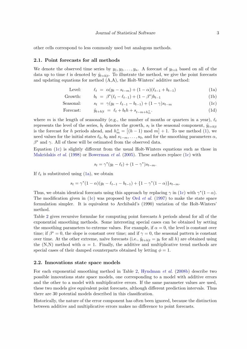
Exponential smoothing methods were originally classified by Pegels’ (1969) taxonomy. Thiswas later extended by Gardner (1985), modified by Hyndman et al. (2002), and extendedagain by Taylor (2003), giving a total of fifteen methods seen in the following table.
Seasonal ComponentTrend N A M
Component (None) (Additive) (Multiplicative)
N (None) N,N N,A N,M
A (Additive) A,N A,A A,M
Ad (Additive damped) Ad,N Ad,A Ad,M
M (Multiplicative) M,N M,A M,M
Md (Multiplicative damped) Md,N Md,A Md,M
Table 1: The fifteen exponential smoothing methods.
Some of these methods are better known under other names. For example, cell (N,N) describesthe simple exponential smoothing (or SES) method, cell (A,N) describes Holt’s linear method,and cell (Ad,N) describes the damped trend method. The additive Holt-Winters’ method isgiven by cell (A,A) and the multiplicative Holt-Winters’ method is given by cell (A,M). The
Journal of Statistical Software 3
other cells correspond to less commonly used but analogous methods.
2.1. Point forecasts for all methods
We denote the observed time series by y1, y2, . . . , yn. A forecast of yt+h based on all of thedata up to time t is denoted by yt+h|t. To illustrate the method, we give the point forecastsand updating equations for method (A,A), the Holt-Winters’ additive method:
Level: `t = α(yt − st−m) + (1− α)(`t−1 + bt−1) (1a)Growth: bt = β∗(`t − `t−1) + (1− β∗)bt−1 (1b)
Seasonal: st = γ(yt − `t−1 − bt−1) + (1− γ)st−m (1c)Forecast: yt+h|t = `t + bth+ st−m+h+
m. (1d)
where m is the length of seasonality (e.g., the number of months or quarters in a year), `trepresents the level of the series, bt denotes the growth, st is the seasonal component, yt+h|tis the forecast for h periods ahead, and h+
m =[(h − 1) mod m
]+ 1. To use method (1), we
need values for the initial states `0, b0 and s1−m, . . . , s0, and for the smoothing parameters α,β∗ and γ. All of these will be estimated from the observed data.
Equation (1c) is slightly different from the usual Holt-Winters equations such as those inMakridakis et al. (1998) or Bowerman et al. (2005). These authors replace (1c) with
st = γ∗(yt − `t) + (1− γ∗)st−m.
If `t is substituted using (1a), we obtain
st = γ∗(1− α)(yt − `t−1 − bt−1) + {1− γ∗(1− α)}st−m.
Thus, we obtain identical forecasts using this approach by replacing γ in (1c) with γ∗(1−α).The modification given in (1c) was proposed by Ord et al. (1997) to make the state spaceformulation simpler. It is equivalent to Archibald’s (1990) variation of the Holt-Winters’method.
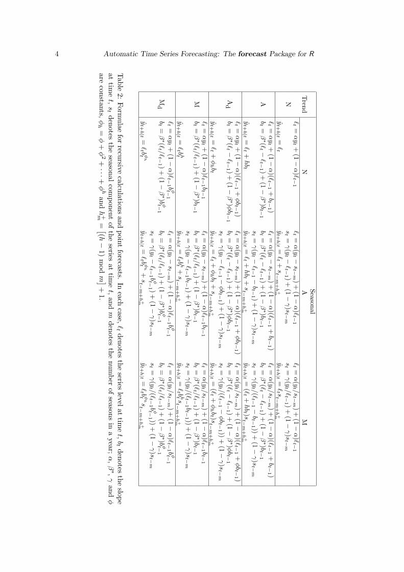
Table 2 gives recursive formulae for computing point forecasts h periods ahead for all of theexponential smoothing methods. Some interesting special cases can be obtained by settingthe smoothing parameters to extreme values. For example, if α = 0, the level is constant overtime; if β∗ = 0, the slope is constant over time; and if γ = 0, the seasonal pattern is constantover time. At the other extreme, naıve forecasts (i.e., yt+h|t = yt for all h) are obtained usingthe (N,N) method with α = 1. Finally, the additive and multiplicative trend methods arespecial cases of their damped counterparts obtained by letting φ = 1.
2.2. Innovations state space models
For each exponential smoothing method in Table 2, Hyndman et al. (2008b) describe twopossible innovations state space models, one corresponding to a model with additive errorsand the other to a model with multiplicative errors. If the same parameter values are used,these two models give equivalent point forecasts, although different prediction intervals. Thusthere are 30 potential models described in this classification.
Historically, the nature of the error component has often been ignored, because the distinctionbetween additive and multiplicative errors makes no difference to point forecasts.
4 Automatic Time Series Forecasting: The forecast Package for R
SeasonalT
rendN
AM
`t
=αyt +
(1−α
)`t−
1`t
=α
(yt −
st−m
)+
(1−α
)`t−
1`t
=α
(yt /s
t−m
)+
(1−α
)`t−
1
Nst
=γ(y
t −`t−
1 )+
(1−γ)s
t−m
st
=γ(y
t /`t−
1 )+
(1−γ)s
t−m
yt+h|t
=`t
yt+h|t
=`t +
st−m
+h+m
yt+h|t
=`t st−m
+h+m
`t
=αyt +
(1−α
)(`t−
1+bt−
1 )`t
=α
(yt −
st−m
)+
(1−α
)(`t−
1+bt−
1 )`t
=α
(yt /s
t−m
)+
(1−α
)(`t−
1+bt−
1 )A
bt
=β∗(`
t −`t−
1 )+
(1−β∗)b
t−1
bt
=β∗(`
t −`t−
1 )+
(1−β∗)b
t−1
bt
=β∗(`
t −`t−
1 )+
(1−β∗)b
t−1
st
=γ(y
t −`t−
1 −bt−
1 )+
(1−γ)s
t−m
st
=γ(y
t /(`t−
1 −bt−
1 ))+
(1−γ)s
t−m
yt+h|t
=`t +
hbt
yt+h|t
=`t +
hbt +
st−m
+h+m
yt+h|t
=(`t +
hbt )s
t−m
+h+m
`t
=αyt +
(1−α
)(`t−
1+φbt−
1 )`t
=α
(yt −
st−m
)+
(1−α
)(`t−
1+φbt−
1 )`t
=α
(yt /s
t−m
)+
(1−α
)(`t−
1+φbt−
1 )A
dbt
=β∗(`
t −`t−
1 )+
(1−β∗)φ
bt−
1bt
=β∗(`
t −`t−
1 )+
(1−β∗)φ
bt−
1bt
=β∗(`
t −`t−
1 )+
(1−β∗)φ
bt−
1
st
=γ(y
t −`t−
1 −φbt−
1 )+
(1−γ)s
t−m
st
=γ(y
t /(`t−
1 −φbt−
1 ))+
(1−γ)s
t−m
yt+h|t
=`t +
φhbt
yt+h|t
=`t +
φhbt +
st−m
+h+m
yt+h|t
=(`t +
φhbt )s
t−m
+h+m
`t
=αyt +
(1−α
)`t−
1 bt−
1`t
=α
(yt −
st−m
)+
(1−α
)`t−
1 bt−
1`t
=α
(yt /s
t−m
)+
(1−α
)`t−
1 bt−
1
Mbt
=β∗(`
t /`t−
1 )+
(1−β∗)b
t−1
bt
=β∗(`
t /`t−
1 )+
(1−β∗)b
t−1
bt
=β∗(`
t /`t−
1 )+
(1−β∗)b
t−1
st
=γ(y
t −`t−
1 bt−
1 )+
(1−γ)s
t−m
st
=γ(y
t /(`t−
1 bt−
1 ))+
(1−γ)s
t−m
yt+h|t
=`t bht
yt+h|t
=`t bht
+st−m
+h+m
yt+h|t
=`t bhtst−m
+h+m
`t
=αyt +
(1−α
)`t−
1 bφt−
1`t
=α
(yt −
st−m
)+
(1−α
)`t−
1 bφt−
1`t
=α
(yt /s
t−m
)+
(1−α
)`t−
1 bφt−
1
Md
bt
=β∗(`
t /`t−
1 )+
(1−β∗)b
φt−1
bt
=β∗(`
t /`t−
1 )+
(1−β∗)b
φt−1
bt
=β∗(`
t /`t−
1 )+
(1−β∗)b
φt−1
st
=γ(y
t −`t−
1 bφt−
1 )+
(1−γ)s
t−m
st
=γ(y
t /(`t−
1 bφt−
1 ))+
(1−γ)s
t−m
yt+h|t
=`t bφ
ht
yt+h|t
=`t bφ
ht
+st−m
+h+m
yt+h|t
=`t bφ
htst−m
+h+m
Table
2:Form
ulaefor
recursivecalculations
andpoint
forecasts.In
eachcase,
`t
denotesthe
serieslevelat
timet,bt
denotesthe
slopeat
timet,st
denotesthe
seasonalcom
ponentof
theseries
attim
et,
andm
denotesthe
number
ofseasons
ina
year;α
,β∗,γ
andφ
areconstants,
φh
=φ
+φ
2+···+
φh
andh
+m= [(h
−1)
mod
m ]+
1.
Journal of Statistical Software 5
We are careful to distinguish exponential smoothing methods from the underlying state spacemodels. An exponential smoothing method is an algorithm for producing point forecasts only.The underlying stochastic state space model gives the same point forecasts, but also providesa framework for computing prediction intervals and other properties.To distinguish the models with additive and multiplicative errors, we add an extra letter tothe front of the method notation. The triplet (E,T,S) refers to the three components: error,trend and seasonality. So the model ETS(A,A,N) has additive errors, additive trend andno seasonality—in other words, this is Holt’s linear method with additive errors. Similarly,ETS(M,Md,M) refers to a model with multiplicative errors, a damped multiplicative trendand multiplicative seasonality. The notation ETS(·,·,·) helps in remembering the order inwhich the components are specified.Once a model is specified, we can study the probability distribution of future values of theseries and find, for example, the conditional mean of a future observation given knowledgeof the past. We denote this as µt+h|t = E(yt+h | xt), where xt contains the unobservedcomponents such as `t, bt and st. For h = 1 we use µt ≡ µt+1|t as a shorthand notation.For many models, these conditional means will be identical to the point forecasts given inTable 2, so that µt+h|t = yt+h|t. However, for other models (those with multiplicative trendor multiplicative seasonality), the conditional mean and the point forecast will differ slightlyfor h ≥ 2.We illustrate these ideas using the damped trend method of Gardner and McKenzie (1985).
Additive error model: ETS(A,Ad,N)
Let µt = yt = `t−1 + bt−1 denote the one-step forecast of yt assuming that we know the valuesof all parameters. Also, let εt = yt − µt denote the one-step forecast error at time t. Fromthe equations in Table 2, we find that
yt = `t−1 + φbt−1 + εt (2)`t = `t−1 + φbt−1 + αεt (3)bt = φbt−1 + β∗(`t − `t−1 − φbt−1) = φbt−1 + αβ∗εt. (4)
We simplify the last expression by setting β = αβ∗. The three equations above constitute astate space model underlying the damped Holt’s method. Note that it is an innovations statespace model (Anderson and Moore 1979; Aoki 1987) because the same error term appears ineach equation. We can write it in standard state space notation by defining the state vectoras xt = (`t, bt)′ and expressing (2)–(4) as
yt = [1 φ]xt−1 + εt (5a)
xt =[
1 φ0 φ
]xt−1 +
[αβ
]εt. (5b)
The model is fully specified once we state the distribution of the error term εt. Usually weassume that these are independent and identically distributed, following a normal distributionwith mean 0 and variance σ2, which we write as εt ∼ NID(0, σ2).
Multiplicative error model: ETS(M,Ad,N)
A model with multiplicative error can be derived similarly, by first setting εt = (yt − µt)/µt,so that εt is the relative error. Then, following a similar approach to that for additive errors,
6 Automatic Time Series Forecasting: The forecast Package for R
we find
yt = (`t−1 + φbt−1)(1 + εt)`t = (`t−1 + φbt−1)(1 + αεt)bt = φbt−1 + β(`t−1 + φbt−1)εt,
or
yt = [1 φ]xt−1(1 + εt)
xt =[
1 φ0 φ
]xt−1 + [1 φ]xt−1
[αβ
]εt.
Again we assume that εt ∼ NID(0, σ2).
Of course, this is a nonlinear state space model, which is usually considered difficult to handlein estimating and forecasting. However, that is one of the many advantages of the innovationsform of state space models — we can still compute forecasts, the likelihood and predictionintervals for this nonlinear model with no more effort than is required for the additive errormodel.
2.3. State space models for all exponential smoothing methods
There are similar state space models for all 30 exponential smoothing variations. The generalmodel involves a state vector xt = (`t, bt, st, st−1, . . . , st−m+1)′ and state space equations ofthe form
yt = w(xt−1) + r(xt−1)εt (6a)xt = f(xt−1) + g(xt−1)εt (6b)
where {εt} is a Gaussian white noise process with mean zero and variance σ2, and µt =w(xt−1). The model with additive errors has r(xt−1) = 1, so that yt = µt + εt. The modelwith multiplicative errors has r(xt−1) = µt, so that yt = µt(1 + εt). Thus, εt = (yt − µt)/µt
is the relative error for the multiplicative model. The models are not unique. Clearly, anyvalue of r(xt−1) will lead to identical point forecasts for yt.
All of the methods in Table 2 can be written in the form (6a) and (6b). The specific form foreach model is given in Hyndman et al. (2008b).
Some of the combinations of trend, seasonality and error can occasionally lead to numeri-cal difficulties; specifically, any model equation that requires division by a state componentcould involve division by zero. This is a problem for models with additive errors and eithermultiplicative trend or multiplicative seasonality, as well as for the model with multiplicativeerrors, multiplicative trend and additive seasonality. These models should therefore be usedwith caution.
The multiplicative error models are useful when the data are strictly positive, but are notnumerically stable when the data contain zeros or negative values. So when the time series isnot strictly positive, only the six fully additive models may be applied.
The point forecasts given in Table 2 are easily obtained from these models by iterating equa-tions (6a) and (6b) for t = n + 1, n + 2, . . . , n + h, setting εn+j = 0 for j = 1, . . . , h. In

Journal of Statistical Software 7
most cases (notable exceptions being models with multiplicative seasonality or multiplicativetrend for h ≥ 2), the point forecasts can be shown to be equal to µt+h|t = E(yt+h | xt), theconditional expectation of the corresponding state space model.The models also provide a means of obtaining prediction intervals. In the case of the linearmodels, where the forecast distributions are normal, we can derive the conditional variancevt+h|t = VAR(yt+h | xt) and obtain prediction intervals accordingly. This approach also worksfor many of the nonlinear models. Detailed derivations of the results for many models aregiven in Hyndman et al. (2005b).A more direct approach that works for all of the models is to simply simulate many futuresample paths conditional on the last estimate of the state vector, xt. Then prediction intervalscan be obtained from the percentiles of the simulated sample paths. Point forecasts can alsobe obtained in this way by taking the average of the simulated values at each future timeperiod. An advantage of this approach is that we generate an estimate of the completepredictive distribution, which is especially useful in applications such as inventory planning,where expected costs depend on the whole distribution.
2.4. Estimation
In order to use these models for forecasting, we need to know the values of x0 and theparameters α, β, γ and φ. It is easy to compute the likelihood of the innovations state spacemodel (6), and so obtain maximum likelihood estimates. Ord et al. (1997) show that
L∗(θ,x0) = n log( n∑
t=1
ε2t
)+ 2
n∑t=1
log |r(xt−1)| (7)
is equal to twice the negative logarithm of the likelihood function (with constant termseliminated), conditional on the parameters θ = (α, β, γ, φ)′ and the initial states x0 =(`0, b0, s0, s−1, . . . , s−m+1)′, where n is the number of observations. This is easily computedby simply using the recursive equations in Table 2. Unlike state space models with multiplesources of error, we do not need to use the Kalman filter to compute the likelihood.The parameters θ and the initial states x0 can be estimated by minimizing L∗. Most imple-mentations of exponential smoothing use an ad hoc heuristic scheme to estimate x0. However,with modern computers, there is no reason why we cannot estimate x0 along with θ, and theresulting forecasts are often substantially better when we do.We constrain the initial states x0 so that the seasonal indices add to zero for additive sea-sonality, and add to m for multiplicative seasonality. There have been several suggestions forrestricting the parameter space for α, β and γ. The traditional approach is to ensure thatthe various equations can be interpreted as weighted averages, thus requiring α, β∗ = β/α,γ∗ = γ/(1− α) and φ to all lie within (0, 1). This suggests
0 < α < 1, 0 < β < α, 0 < γ < 1− α, and 0 < φ < 1.
However, Hyndman et al. (2008a) show that these restrictions are usually stricter than nec-essary (although in a few cases they are not restrictive enough).
2.5. Model selection
Forecast accuracy measures such as mean squared error (MSE) can be used for selecting amodel for a given set of data, provided the errors are computed from data in a hold-out set
8 Automatic Time Series Forecasting: The forecast Package for R
and not from the same data as were used for model estimation. However, there are oftentoo few out-of-sample errors to draw reliable conclusions. Consequently, a penalized methodbased on the in-sample fit is usually better.
One such approach uses a penalized likelihood such as Akaike’s Information Criterion:
AIC = L∗(θ, x0) + 2q,
where q is the number of parameters in θ plus the number of free states in x0, and θ and x0
denote the estimates of θ and x0. We select the model that minimizes the AIC amongst allof the models that are appropriate for the data.
The AIC also provides a method for selecting between the additive and multiplicative errormodels. The point forecasts from the two models are identical so that standard forecastaccuracy measures such as the MSE or mean absolute percentage error (MAPE) are unableto select between the error types. The AIC is able to select between the error types becauseit is based on likelihood rather than one-step forecasts.
Obviously, other model selection criteria (such as the BIC) could also be used in a similarmanner.
2.6. Automatic forecasting
We combine the preceding ideas to obtain a robust and widely applicable automatic forecastingalgorithm. The steps involved are summarized below.
1. For each series, apply all models that are appropriate, optimizing the parameters (bothsmoothing parameters and the initial state variable) of the model in each case.
2. Select the best of the models according to the AIC.3. Produce point forecasts using the best model (with optimized parameters) for as many
steps ahead as required.4. Obtain prediction intervals for the best model either using the analytical results of
Hyndman et al. (2005b), or by simulating future sample paths for {yn+1, . . . , yn+h} andfinding the α/2 and 1−α/2 percentiles of the simulated data at each forecasting horizon.If simulation is used, the sample paths may be generated using the normal distributionfor errors (parametric bootstrap) or using the resampled errors (ordinary bootstrap).
Hyndman et al. (2002) applied this automatic forecasting strategy to the M-competition data(Makridakis et al. 1982) and the IJF-M3 competition data (Makridakis and Hibon 2000) usinga restricted set of exponential smoothing models, and demonstrated that the methodology isparticularly good at short term forecasts (up to about 6 periods ahead), and especially forseasonal short-term series (beating all other methods in the competitions for these series).
3. ARIMA models
A common obstacle for many people in using Autoregressive Integrated Moving Average(ARIMA) models for forecasting is that the order selection process is usually consideredsubjective and difficult to apply. But it does not have to be. There have been severalattempts to automate ARIMA modelling in the last 25 years.
Hannan and Rissanen (1982) proposed a method to identify the order of an ARMA modelfor a stationary series. In their method the innovations can be obtained by fitting a long
Journal of Statistical Software 9
autoregressive model to the data, and then the likelihood of potential models is computed viaa series of standard regressions. They established the asymptotic properties of the procedureunder very general conditions.
Gomez (1998) extended the Hannan-Rissanen identification method to include multiplicativeseasonal ARIMA model identification. Gomez and Maravall (1998) implemented this auto-matic identification procedure in the software TRAMO and SEATS. For a given series, thealgorithm attempts to find the model with the minimum BIC.
Liu (1989) proposed a method for identification of seasonal ARIMA models using a filteringmethod and certain heuristic rules; this algorithm is used in the SCA-Expert software. An-other approach is described by Melard and Pasteels (2000) whose algorithm for univariateARIMA models also allows intervention analysis. It is implemented in the software package“Time Series Expert” (TSE-AX).
Other algorithms are in use in commercial software, although they are not documented inthe public domain literature. In particular, Forecast Pro (Goodrich 2000) is well-known forits excellent automatic ARIMA algorithm which was used in the M3-forecasting competition(Makridakis and Hibon 2000). Another proprietary algorithm is implemented in Autobox(Reilly 2000). Ord and Lowe (1996) provide an early review of some of the commercialsoftware that implement automatic ARIMA forecasting.
3.1. Choosing the model order using unit root tests and the AIC
A non-seasonal ARIMA(p, d, q) process is given by
φ(B)(1−Bd)yt = c+ θ(B)εt
where {εt} is a white noise process with mean zero and variance σ2, B is the backshiftoperator, and φ(z) and θ(z) are polynomials of order p and q respectively. To ensure causalityand invertibility, it is assumed that φ(z) and θ(z) have no roots for |z| < 1 (Brockwell andDavis 1991). If c 6= 0, there is an implied polynomial of order d in the forecast function.
The seasonal ARIMA(p, d, q)(P,D,Q)m process is given by
Φ(Bm)φ(B)(1−Bm)D(1−B)dyt = c+ Θ(Bm)θ(B)εt
where Φ(z) and Θ(z) are polynomials of orders P and Q respectively, each containing no rootsinside the unit circle. If c 6= 0, there is an implied polynomial of order d+D in the forecastfunction.
The main task in automatic ARIMA forecasting is selecting an appropriate model order, thatis the values p, q, P , Q, D, d. If d and D are known, we can select the orders p, q, P and Qvia an information criterion such as the AIC:
AIC = −2 log(L) + 2(p+ q + P +Q+ k)
where k = 1 if c 6= 0 and 0 otherwise, and L is the maximized likelihood of the model fitted tothe differenced data (1−Bm)D(1−B)dyt. The likelihood of the full model for yt is not actuallydefined and so the value of the AIC for different levels of differencing are not comparable.
One solution to this difficulty is the “diffuse prior” approach which is outlined in Durbinand Koopman (2001) and implemented in the arima() function (Ripley 2002) in R. In this
10 Automatic Time Series Forecasting: The forecast Package for R
approach, the initial values of the time series (before the observed values) are assumed tohave mean zero and a large variance. However, choosing d and D by minimizing the AICusing this approach tends to lead to over-differencing. For forecasting purposes, we believeit is better to make as few differences as possible because over-differencing harms forecasts(Smith and Yadav 1994) and widens prediction intervals. (Although, see Hendry 1997, for acontrary view.)Consequently, we need some other approach to choose d and D. We prefer unit-root tests.However, most unit-root tests are based on a null hypothesis that a unit root exists whichbiases results towards more differences rather than fewer differences. For example, variationson the Dickey-Fuller test (Dickey and Fuller 1981) all assume there is a unit root at lag 1, andthe HEGY test of Hylleberg et al. (1990) is based on a null hypothesis that there is a seasonalunit root. Instead, we prefer unit-root tests based on a null hypothesis of no unit-root.For non-seasonal data, we consider ARIMA(p, d, q) models where d is selected based on suc-cessive KPSS unit-root tests (Kwiatkowski et al. 1992). That is, we test the data for a unitroot; if the test result is significant, we test the differenced data for a unit root; and so on.We stop this procedure when we obtain our first insignificant result.For seasonal data, we consider ARIMA(p, d, q)(P,D,Q)m models where m is the seasonalfrequency and D = 0 or D = 1 depending on an extended Canova-Hansen test (Canova andHansen 1995). Canova and Hansen only provide critical values for 2 < m < 13. In ourimplementation of their test, we allow any value of m > 1. Let Cm be the critical value forseasonal period m. We plotted Cm against m for values of m up to 365 and noted that theyfit the line Cm = 0.269m0.928 almost exactly. So for m > 12, we use this simple expression toobtain the critical value.We note in passing that the null hypothesis for the Canova-Hansen test is not an ARIMAmodel as it includes seasonal dummy terms. It is a test for whether the seasonal patternchanges sufficiently over time to warrant a seasonal unit root, or whether a stable seasonalpattern modelled using fixed dummy variables is more appropriate. Nevertheless, we havefound that the test is still useful for choosing D in a strictly ARIMA framework (i.e., withoutseasonal dummy variables). If a stable seasonal pattern is selected (i.e., the null hypothesis isnot rejected), the seasonality is effectively handled by stationary seasonal AR and MA terms.After D is selected, we choose d by applying successive KPSS unit-root tests to the seasonallydifferenced data (if D = 1) or the original data (if D = 0). Once d (and possibly D) areselected, we proceed to select the values of p, q, P and Q by minimizing the AIC. We allowc 6= 0 for models where d+D < 2.
3.2. A step-wise procedure for traversing the model space
Suppose we have seasonal data and we consider ARIMA(p, d, q)(P,D,Q)m models where pand q can take values from 0 to 3, and P and Q can take values from 0 to 1. When c = 0there is a total of 288 possible models, and when c 6= 0 there is a total of 192 possible models,giving 480 models altogether. If the values of p, d, q, P , D and Q are allowed to range morewidely, the number of possible models increases rapidly. Consequently, it is often not feasibleto simply fit every potential model and choose the one with the lowest AIC. Instead, we needa way of traversing the space of models efficiently in order to arrive at the model with thelowest AIC value.We propose a step-wise algorithm as follows.

Journal of Statistical Software 11
Step 1: We try four possible models to start with.
� ARIMA(2, d, 2) if m = 1 and ARIMA(2, d, 2)(1, D, 1) if m > 1.
� ARIMA(0, d, 0) if m = 1 and ARIMA(0, d, 0)(0, D, 0) if m > 1.
� ARIMA(1, d, 0) if m = 1 and ARIMA(1, d, 0)(1, D, 0) if m > 1.
� ARIMA(0, d, 1) if m = 1 and ARIMA(0, d, 1)(0, D, 1) if m > 1.
If d+D ≤ 1, these models are fitted with c 6= 0. Otherwise, we set c = 0. Of these fourmodels, we select the one with the smallest AIC value. This is called the“current”modeland is denoted by ARIMA(p, d, q) if m = 1 or ARIMA(p, d, q)(P,D,Q)m if m > 1.
Step 2: We consider up to thirteen variations on the current model:
� where one of p, q, P and Q is allowed to vary by ±1 from the current model;
� where p and q both vary by ±1 from the current model;
� where P and Q both vary by ±1 from the current model;
� where the constant c is included if the current model has c = 0 or excluded if thecurrent model has c 6= 0.
Whenever a model with lower AIC is found, it becomes the new “current” model andthe procedure is repeated. This process finishes when we cannot find a model close tothe current model with lower AIC.
There are several constraints on the fitted models to avoid problems with convergence or nearunit-roots. The constraints are outlined below.
� The values of p and q are not allowed to exceed specified upper bounds (with defaultvalues of 5 in each case).
� The values of P and Q are not allowed to exceed specified upper bounds (with defaultvalues of 2 in each case).
� We reject any model which is “close” to non-invertible or non-causal. Specifically, wecompute the roots of φ(B)Φ(B) and θ(B)Θ(B). If either have a root that is smallerthan 1.001 in absolute value, the model is rejected.
� If there are any errors arising in the non-linear optimization routine used for estimation,the model is rejected. The rationale here is that any model that is difficult to fit isprobably not a good model for the data.
The algorithm is guaranteed to return a valid model because the model space is finite and atleast one of the starting models will be accepted (the model with no AR or MA parameters).The selected model is used to produce forecasts.
3.3. Comparisons with exponential smoothing
There is a widespread myth that ARIMA models are more general than exponential smooth-ing. This is not true. The two classes of models overlap. The linear exponential smoothingmodels are all special cases of ARIMA models—the equivalences are discussed in Hyndman
12 Automatic Time Series Forecasting: The forecast Package for R
et al. (2008a). However, the non-linear exponential smoothing models have no equivalentARIMA counterpart. On the other hand, there are many ARIMA models which have noexponential smoothing counterpart. Thus, the two model classes overlap and are complimen-tary; each has its strengths and weaknesses.
The exponential smoothing state space models are all non-stationary. Models with seasonalityor non-damped trend (or both) have two unit roots; all other models—that is, non-seasonalmodels with either no trend or damped trend—have one unit root. It is possible to definea stationary model with similar characteristics to exponential smoothing, but this is notnormally done. The philosophy of exponential smoothing is that the world is non-stationary.So if a stationary model is required, ARIMA models are better.
One advantage of the exponential smoothing models is that they can be non-linear. Sotime series that exhibit non-linear characteristics including heteroscedasticity may be bettermodelled using exponential smoothing state space models.
For seasonal data, there are many more ARIMA models than the 30 possible models in theexponential smoothing class of Section 2. It may be thought that the larger model classis advantageous. However, the results in Hyndman et al. (2002) show that the exponentialsmoothing models performed better than the ARIMA models for the seasonal M3 competitiondata. (For the annual M3 data, the ARIMA models performed better.) In a discussion ofthese results, Hyndman (2001) speculates that the larger model space of ARIMA modelsactually harms forecasting performance because it introduces additional uncertainty. Thesmaller exponential smoothing class is sufficiently rich to capture the dynamics of almost allreal business and economic time series.
4. The forecast package
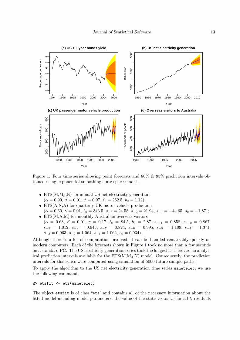
The algorithms and modelling frameworks for automatic univariate time series forecasting areimplemented in the forecast package in R. We illustrate the methods using the following fourreal time series shown in Figure 1.
� Figure 1(a) shows 125 monthly US government bond yields (percent per annum) fromJanuary 1994 to May 2004.
� Figure 1(b) displays 55 observations of annual US net electricity generation (billionkwh) for 1949 through 2003.
� Figure 1(c) presents 113 quarterly observations of passenger motor vehicle productionin the U.K. (thousands of cars) for the first quarter of 1977 through the first quarter of2005.
� Figure 1(d) shows 240 monthly observations of the number of short term overseas visitorsto Australia from May 1985 to April 2005.
4.1. Implementation of the automatic exponential smoothing algorithm
The innovations state space modelling framework described in Section 2 is implemented viathe ets() function in the forecast package. The models chosen via the algorithm for the fourdata sets were:
� ETS(A,Ad,N) for monthly US 10-year bonds yield(α = 0.99, β = 0.12, φ = 0.80, `0 = 5.30, b0 = 0.71);
Journal of Statistical Software 13
(a) US 10−year bonds yield
Year
Per
cent
age
per
annu
m
1994 1996 1998 2000 2002 2004 2006
23
45
67
8(b) US net electricity generation
Year
Bill
ion
kwh
1950 1960 1970 1980 1990 2000 2010
1000
3000
5000
(c) UK passenger motor vehicle production
Year
Tho
usan
ds o
f car
s
1980 1985 1990 1995 2000 2005
200
300
400
500
(d) Overseas visitors to Australia
Year
Tho
usan
ds o
f peo
ple
1985 1990 1995 2000 2005
200
400
600
800
Figure 1: Four time series showing point forecasts and 80% & 95% prediction intervals ob-tained using exponential smoothing state space models.
� ETS(M,Md,N) for annual US net electricity generation(α = 0.99, β = 0.01, φ = 0.97, `0 = 262.5, b0 = 1.12);
� ETS(A,N,A) for quarterly UK motor vehicle production(α = 0.60, γ = 0.01, `0 = 343.5, s−3 = 24.58, s−2 = 21.94, s−1 = −44.65, s0 = −1.87);
� ETS(M,A,M) for monthly Australian overseas visitors(α = 0.68, β = 0.01, γ = 0.17, `0 = 84.5, b0 = 2.87, s−11 = 0.858, s−10 = 0.867,s−9 = 1.012, s−8 = 0.943, s−7 = 0.824, s−6 = 0.995, s−5 = 1.109, s−4 = 1.371,s−3 = 0.963, s−2 = 1.064, s−1 = 1.062, s0 = 0.934).
Although there is a lot of computation involved, it can be handled remarkably quickly onmodern computers. Each of the forecasts shown in Figure 1 took no more than a few secondson a standard PC. The US electricity generation series took the longest as there are no analyt-ical prediction intervals available for the ETS(M,Md,N) model. Consequently, the predictionintervals for this series were computed using simulation of 5000 future sample paths.
To apply the algorithm to the US net electricity generation time series usnetelec, we usethe following command.
R> etsfit <- ets(usnetelec)
The object etsfit is of class “ets” and contains all of the necessary information about thefitted model including model parameters, the value of the state vector xt for all t, residuals

14 Automatic Time Series Forecasting: The forecast Package for R
and so on. Printing the etsfit object shows the main items of interest.
R> etsfitETS(M,Md,N)
Call:ets(y = usnetelec)
Smoothing parameters:alpha = 0.99beta = 0.01phi = 0.965
Initial states:l = 262.5316b = 1.1207
sigma: 0.0239
AIC AICc BIC628.82 630.05 638.86
Some goodness-of-fit measures (defined in Hyndman and Koehler 2006) are obtained usingaccuracy().
R> accuracy(etsfit)ME RMSE MAE MPE MAPE MASE
-1.3934 49.5024 33.7931 -0.0572 1.8129 0.4788
There are also coef(), plot(), summary(), residuals(), fitted() and simulate() meth-ods for objects of class “ets”. The plot() function shows time plots of the original time seriesalong with the extracted components (level, growth and seasonal).
The forecast() function computes the required forecasts which are then plotted as in Fig-ure 1(b).
R> fcast <- forecast(etsfit)R> plot(fcast)
Printing the fcast object gives a table showing the prediction intervals.
R> fcastPoint Forecast Lo 80 Hi 80 Lo 95 Hi 95
2004 3909 3784 4032 3721 40902005 3969 3793 4142 3707 42282006 4029 3808 4241 3695 43592007 4087 3828 4336 3705 44912008 4144 3842 4425 3709 46052009 4200 3870 4515 3718 4712
Journal of Statistical Software 15
2010 4254 3893 4602 3729 48112011 4308 3908 4684 3728 49092012 4360 3938 4765 3738 50072013 4410 3955 4843 3759 5096
The ets() function also provides the useful feature of applying a fitted model to a new dataset. For example, we could withhold 10 observations from the usnetelec data set whenfitting, then compute the one-step forecast errors for the out-of-sample data.
R> fit <- ets(usnetelec[1:45])R> test <- ets(usnetelec[46:55], model = fit)R> accuracy(test)
We can also look at the measures of forecast accuracy where the forecasts are based on onlythe fitting data.
R> accuracy(forecast(fit,10), usnetelec[46:55])
4.2. The HoltWinters() function
There is another implementation of exponential smoothing in R via the HoltWinters() func-tion (Meyer 2002) in the stats package. It implements only the (N,N), (A,N), (A,A) and(A,M) methods. The initial states x0 are fixed using a heuristic algorithm. Because of theway the initial states are estimated, a full three years of seasonal data are required to imple-ment the seasonal forecasts using HoltWinters(). (See Hyndman and Kostenko (2007) forthe minimal sample size required.) The smoothing parameters are optimized by minimizingthe average squared prediction errors, which is equivalent to minimizing (7) in the case ofadditive errors.There is a predict() method for the resulting object which can produce point forecasts andprediction intervals. Although it is nowhere documented, it appears that the prediction inter-vals produced by predict() for an object of class HoltWinters are based on an equivalentARIMA model in the case of the (N,N), (A,N) and (A,A) methods, assuming additive er-rors. These prediction intervals are equivalent to the prediction intervals that arise from the(A,N,N), (A,A,N) and (A,A,A) state space models. For the (A,M) method, the predictioninterval provided by predict() appears to be based on Chatfield and Yar (1991) which isan approximation to the true prediction interval arising from the (A,A,M) model. Predictionintervals with multiplicative errors are not possible using the HoltWinters() function.
4.3. Implementation of the automatic ARIMA algorithm
The algorithm of Section 3 is applied to the same four time series. Unlike the exponentialsmoothing algorithm, the ARIMA class of models assumes homoscedasticity, which is notalways appropriate. Consequently, transformations are sometimes necessary. For these fourtime series, we model the raw data for series (a)–(c), but the logged data for series (d). Theprediction intervals are back-transformed with the point forecasts to preserve the probabilitycoverage.To apply this algorithm to the US net electricity generation time series usnetelec, we usethe following commands.
16 Automatic Time Series Forecasting: The forecast Package for R
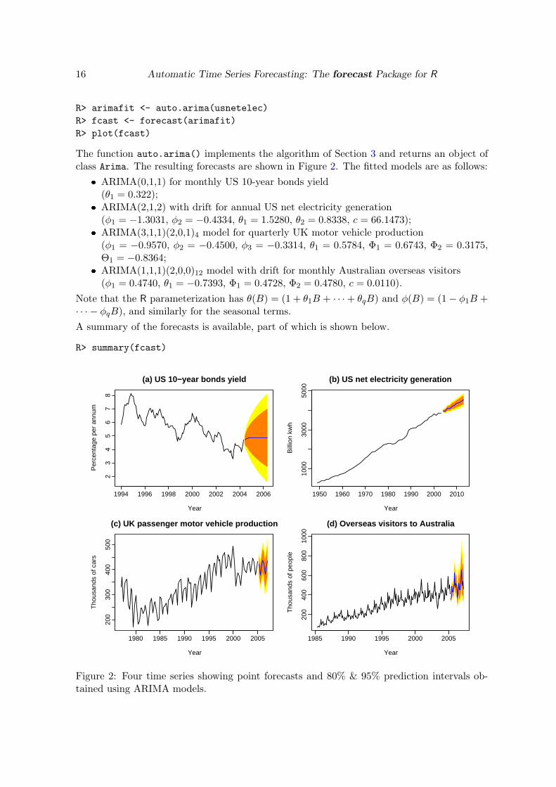
R> arimafit <- auto.arima(usnetelec)R> fcast <- forecast(arimafit)R> plot(fcast)
The function auto.arima() implements the algorithm of Section 3 and returns an object ofclass Arima. The resulting forecasts are shown in Figure 2. The fitted models are as follows:
� ARIMA(0,1,1) for monthly US 10-year bonds yield(θ1 = 0.322);
� ARIMA(2,1,2) with drift for annual US net electricity generation(φ1 = −1.3031, φ2 = −0.4334, θ1 = 1.5280, θ2 = 0.8338, c = 66.1473);
� ARIMA(3,1,1)(2,0,1)4 model for quarterly UK motor vehicle production(φ1 = −0.9570, φ2 = −0.4500, φ3 = −0.3314, θ1 = 0.5784, Φ1 = 0.6743, Φ2 = 0.3175,Θ1 = −0.8364;
� ARIMA(1,1,1)(2,0,0)12 model with drift for monthly Australian overseas visitors(φ1 = 0.4740, θ1 = −0.7393, Φ1 = 0.4728, Φ2 = 0.4780, c = 0.0110).
Note that the R parameterization has θ(B) = (1 + θ1B + · · ·+ θqB) and φ(B) = (1− φ1B +· · · − φqB), and similarly for the seasonal terms.A summary of the forecasts is available, part of which is shown below.
R> summary(fcast)
(a) US 10−year bonds yield
Year
Per
cent
age
per
annu
m
1994 1996 1998 2000 2002 2004 2006
23
45
67
8
(b) US net electricity generation
Year
Bill
ion
kwh
1950 1960 1970 1980 1990 2000 2010
1000
3000
5000
(c) UK passenger motor vehicle production
Year
Tho
usan
ds o
f car
s
1980 1985 1990 1995 2000 2005
200
300
400
500
(d) Overseas visitors to Australia
Year
Tho
usan
ds o
f peo
ple
1985 1990 1995 2000 2005
200
400
600
800
1000
Figure 2: Four time series showing point forecasts and 80% & 95% prediction intervals ob-tained using ARIMA models.
Journal of Statistical Software 17
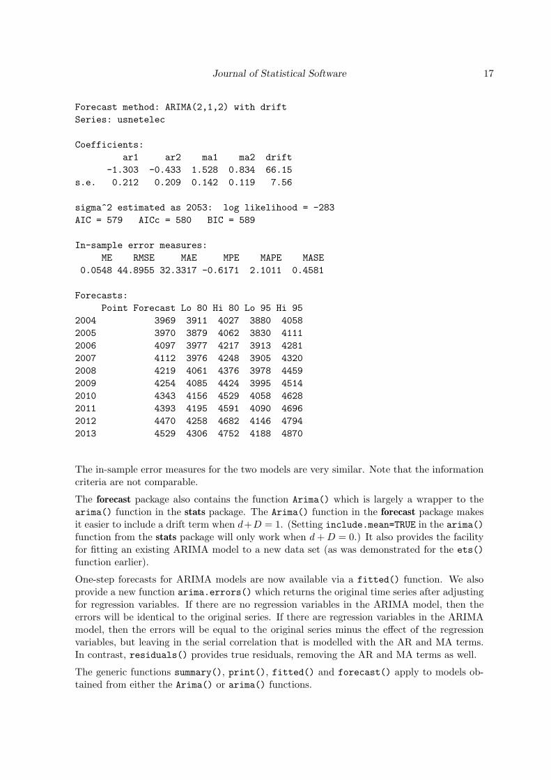
Forecast method: ARIMA(2,1,2) with driftSeries: usnetelec
Coefficients:ar1 ar2 ma1 ma2 drift
-1.303 -0.433 1.528 0.834 66.15s.e. 0.212 0.209 0.142 0.119 7.56
sigma^2 estimated as 2053: log likelihood = -283AIC = 579 AICc = 580 BIC = 589
In-sample error measures:ME RMSE MAE MPE MAPE MASE
0.0548 44.8955 32.3317 -0.6171 2.1011 0.4581
Forecasts:Point Forecast Lo 80 Hi 80 Lo 95 Hi 95
2004 3969 3911 4027 3880 40582005 3970 3879 4062 3830 41112006 4097 3977 4217 3913 42812007 4112 3976 4248 3905 43202008 4219 4061 4376 3978 44592009 4254 4085 4424 3995 45142010 4343 4156 4529 4058 46282011 4393 4195 4591 4090 46962012 4470 4258 4682 4146 47942013 4529 4306 4752 4188 4870
The in-sample error measures for the two models are very similar. Note that the informationcriteria are not comparable.
The forecast package also contains the function Arima() which is largely a wrapper to thearima() function in the stats package. The Arima() function in the forecast package makesit easier to include a drift term when d+D = 1. (Setting include.mean=TRUE in the arima()function from the stats package will only work when d+D = 0.) It also provides the facilityfor fitting an existing ARIMA model to a new data set (as was demonstrated for the ets()function earlier).
One-step forecasts for ARIMA models are now available via a fitted() function. We alsoprovide a new function arima.errors() which returns the original time series after adjustingfor regression variables. If there are no regression variables in the ARIMA model, then theerrors will be identical to the original series. If there are regression variables in the ARIMAmodel, then the errors will be equal to the original series minus the effect of the regressionvariables, but leaving in the serial correlation that is modelled with the AR and MA terms.In contrast, residuals() provides true residuals, removing the AR and MA terms as well.
The generic functions summary(), print(), fitted() and forecast() apply to models ob-tained from either the Arima() or arima() functions.
18 Automatic Time Series Forecasting: The forecast Package for R
4.4. The forecast() function
The forecast() function is generic and has S3 methods for a wide range of time series models.It computes point forecasts and prediction intervals from the time series model. Methods existfor models fitted using ets(), auto.arima(), Arima(), arima(), ar(), HoltWinters() andStructTS().
There is also a method for a ts object. If a time series object is passed as the first argument toforecast(), the function will produce forecasts based on the exponential smoothing algorithmof Section 2.
In most cases, there is an existing predict() function which is intended to do much the samething. Unfortunately, the resulting objects from the predict() function contain differentinformation in each case and so it is not possible to build generic functions (such as plot()and summary()) for the results. So, instead, forecast() acts as a wrapper to predict(),and packages the information obtained in a common format (the forecast class). We alsodefine a default predict() method which is used when no existing predict() function exists,and calls the relevant forecast() function. Thus, predict() methods parallel forecast()methods, but the latter provide consistent output that is more useable.
4.5. The forecast class
The output from the forecast() function is an object of class “forecast” and includes atleast the following information:
� the original series;� point forecasts;� prediction intervals of specified coverage;� the forecasting method used and information about the fitted model;� residuals from the fitted model;� one-step forecasts from the fitted model for the period of the observed data.
There are print(), plot() and summary() methods for the“forecast”class. Figures 1 and 2were produced using the plot() method.
The prediction intervals are, by default, computed for 80% and 95% coverage, although othervalues are possible if requested. Fan charts (Wallis 1999) are possible using the combinationplot(forecast(model.object, fan = TRUE)).
4.6. Other functions
We now briefly describe some of the other features of the forecast package. Each of thefollowing functions produces an object of class “forecast”.
croston() implements Croston’s (1972) method for intermittent demand forecasting. Inthis method, the time series is decomposed into two separate sequences: the non-zerovalues and the time intervals between non-zero values. These are then independentlyforecast using simple exponential smoothing and the forecasts of the original series areobtained as ratios of the two sets of forecasts. No prediction intervals are providedbecause there is no underlying stochastic model (Shenstone and Hyndman 2005).
theta() provides forecasts from the Theta method (Assimakopoulos and Nikolopoulos 2000).
Journal of Statistical Software 19
Hyndman and Billah (2003) showed that these were equivalent to a special case of simpleexponential smoothing with drift.
splinef() gives cubic-spline forecasts, based on fitting a cubic spline to the historical dataand extrapolating it linearly. The details of this method, and the associated predictionintervals, are discussed in Hyndman et al. (2005a).
meanf() returns forecasts based on the historical mean.
rwf() gives “naıve” forecasts equal to the most recent observation assuming a random walkmodel. This function also allows forecasting using a random walk with drift.
In addition, there are some new plotting functions for time series.
tsdisplay() provides a time plot along with an ACF and PACF.
seasonplot() produces a seasonal plot as described in Makridakis et al. (1998).
References
Anderson BDO, Moore JB (1979). Optimal Filtering. Prentice-Hall, Englewood Cliffs.
Aoki M (1987). State Space Modeling of Time Series. Springer-Verlag, Berlin.
Archibald BC (1990). “Parameter Space of the Holt-Winters’ Model.” International Journalof Forecasting, 6, 199–209.
Assimakopoulos V, Nikolopoulos K (2000). “The Theta Model: A Decomposition Approachto Forecasting.” International Journal of Forecasting, 16, 521–530.
Bowerman BL, O’Connell RT, Koehler AB (2005). Forecasting, Time Series and Regression:An Applied Approach. Thomson Brooks/Cole, Belmont CA.
Brockwell PJ, Davis RA (1991). Time Series: Theory and Methods. 2nd edition. Springer-Verlag, New York.
Canova F, Hansen BE (1995). “Are Seasonal Patterns Constant Over Time? A Test forSeasonal Stability.” Journal of Business and Economic Statistics, 13, 237–252.
Chatfield C, Yar M (1991). “Prediction Intervals for Multiplicative Holt-Winters.” Interna-tional Journal of Forecasting, 7, 31–37.
Croston JD (1972). “Forecasting and Stock Control for Intermittent Demands.” OperationalResearch Quarterly, 23(3), 289–304.
Dickey DA, Fuller WA (1981). “Likelihood Ratio Statistics for Autoregressive Time Serieswith a Unit Root.” Econometrica, 49, 1057–1071.
Durbin J, Koopman SJ (2001). Time Series Analysis by State Space Methods. Oxford Uni-versity Press, Oxford.
20 Automatic Time Series Forecasting: The forecast Package for R
Gardner Jr ES (1985). “Exponential Smoothing: The State of the Art.” Journal of Forecasting,4, 1–28.
Gardner Jr ES, McKenzie E (1985). “Forecasting Trends in Time Series.” ManagementScience, 31(10), 1237–1246.
Gomez V (1998). “Automatic Model Identification in the Presence of Missing Observationsand Outliers.” Working paper D-98009, Ministerio de Economıa y Hacienda, DireccionGeneral de Analisis y Programacion Presupuestaria.
Gomez V, Maravall A (1998). “Programs TRAMO and SEATS, Instructions for the Users.”Working paper 97001, Ministerio de Economıa y Hacienda, Direccion General de Analisisy Programacion Presupuestaria.
Goodrich RL (2000). “The Forecast Pro Methodology.” International Journal of Forecasting,16(4), 533–535.
Hannan EJ, Rissanen J (1982). “Recursive Estimation of Mixed Autoregressive-Moving Av-erage Order.” Biometrika, 69(1), 81–94.
Hendry DF (1997). “The Econometrics of Macroeconomic Forecasting.” The Economic Jour-nal, 107(444), 1330–1357.
Hylleberg S, Engle R, Granger C, Yoo B (1990). “Seasonal Integration and Cointegration.”Journal of Econometrics, 44, 215–238.
Hyndman RJ (2001). “It’s Time To Move from ‘What’ To ‘Why’—Comments on the M3-Competition.” International Journal of Forecasting, 17(4), 567–570.
Hyndman RJ (2008a). expsmooth: Data Sets from “Forecasting with Exponential Smoothing”by Hyndman, Koehler, Ord & Snyder (2008). R package version 1.11, URL http://CRAN.R-project.org/package=forecasting.
Hyndman RJ (2008b). fma: Data Sets from “Forecasting: Methods and Applications” ByMakridakis, Wheelwright & Hyndman (1998). R package version 1.11, URL http://CRAN.R-project.org/package=forecasting.
Hyndman RJ (2008c). forecast: Forecasting Functions for Time Series. R package ver-sion 1.11, URL http://CRAN.R-project.org/package=forecasting.
Hyndman RJ (2008d). Mcomp: Data from the M-Competitions. R package version 1.11,URL http://CRAN.R-project.org/package=forecasting.
Hyndman RJ, Akram M, Archibald BC (2008a). “The Admissible Parameter Space for Ex-ponential Smoothing Models.” Annals of the Institute of Statistical Mathematics, 60(2),407–426.
Hyndman RJ, Billah B (2003). “Unmasking the Theta Method.” International Journal ofForecasting, 19(2), 287–290.
Hyndman RJ, King ML, Pitrun I, Billah B (2005a). “Local Linear Forecasts Using CubicSmoothing Splines.” Australian & New Zealand Journal of Statistics, 47(1), 87–99.
Journal of Statistical Software 21
Hyndman RJ, Koehler AB (2006). “Another Look at Measures of Forecast Accuracy.” Inter-national Journal of Forecasting, 22, 679–688.
Hyndman RJ, Koehler AB, Ord JK, Snyder RD (2005b). “Prediction Intervals for ExponentialSmoothing Using Two New Classes of State Space Models.” Journal of Forecasting, 24,17–37.
Hyndman RJ, Koehler AB, Ord JK, Snyder RD (2008b). Forecasting with Exponen-tial Smoothing: The State Space Approach. Springer-Verlag. URL http://www.exponentialsmoothing.net/.
Hyndman RJ, Koehler AB, Snyder RD, Grose S (2002). “A State Space Framework forAutomatic Forecasting Using Exponential Smoothing Methods.” International Journal ofForecasting, 18(3), 439–454.
Hyndman RJ, Kostenko AV (2007). “Minimum Sample Size Requirements for Seasonal Fore-casting Models.” Foresight: The International Journal of Applied Forecasting, 6, 12–15.
Kwiatkowski D, Phillips PC, Schmidt P, Shin Y (1992). “Testing the Null Hypothesis ofStationarity Against the Alternative of a Unit Root.” Journal of Econometrics, 54, 159–178.
Liu LM (1989). “Identification of Seasonal Arima Models Using a Filtering Method.” Com-munications in Statistics: Theory & Methods, 18, 2279–2288.
Makridakis S, Anderson A, Carbone R, Fildes R, Hibon M, Lewandowski R, Newton J, ParzenE, Winkler R (1982). “The Accuracy of Extrapolation (Time Series) Methods: Results ofa Forecasting Competition.” Journal of Forecasting, 1, 111–153.
Makridakis S, Hibon M (2000). “The M3-Competition: Results, Conclusions and Implica-tions.” International Journal of Forecasting, 16, 451–476.
Makridakis S, Wheelwright SC, Hyndman RJ (1998). Forecasting: Methods and Applica-tions. 3rd edition. John Wiley & Sons, New York. URL http://www.robhyndman.info/forecasting/.
Melard G, Pasteels JM (2000). “Automatic ARIMA Modeling Including Intervention, UsingTime Series Expert Software.” International Journal of Forecasting, 16, 497–508.
Meyer D (2002). “Naive Time Series Forecasting Methods.” R News, 2(2), 7–10. URLhttp://CRAN.R-project.org/doc/Rnews/.
Ord JK, Koehler AB, Snyder RD (1997). “Estimation and Prediction for a Class of DynamicNonlinear Statistical Models.” Journal of the American Statistical Association, 92, 1621–1629.
Ord K, Lowe S (1996). “Automatic Forecasting.” The American Statistician, 50(1), 88–94.
Pegels CC (1969). “Exponential Forecasting: Some New Variations.” Management Science,15(5), 311–315.
22 Automatic Time Series Forecasting: The forecast Package for R
R Development Core Team (2008). R: A Language and Environment for Statistical Computing.R Foundation for Statistical Computing, Vienna, Austria. ISBN 3-900051-07-0, URL http://www.R-project.org/.
Reilly D (2000). “The Autobox System.” International Journal of Forecasting, 16(4), 531–533.
Ripley BD (2002). “Time Series in R 1.5.0.” R News, 2(2), 2–7. URL http://CRAN.R-project.org/doc/Rnews/.
Shenstone L, Hyndman RJ (2005). “Stochastic Models Underlying Croston’s Method forIntermittent Demand Forecasting.” Journal of Forecasting, 24, 389–402.
Smith J, Yadav S (1994). “Forecasting Costs Incurred from Unit Differencing FractionallyIntegrated Processes.” International Journal of Forecasting, 10(4), 507–514.
Taylor JW (2003). “Exponential Smoothing with a Damped Multiplicative Trend.” Interna-tional Journal of Forecasting, 19, 715–725.
Wallis KF (1999). “Asymmetric Density Forecasts of Inflation and the Bank of England’s FanChart.” National Institute Economic Review, 167(1), 106–112.
Affiliation:
Rob J. HyndmanDepartment of Econometrics & Business StatisticsMonash UniversityClayton VIC 3800, AustraliaE-mail: [email protected]: http://www.robhyndman.info
Yeasmin KhandakarDepartment of Econometrics & Business StatisticsMonash UniversityClayton VIC 3800, AustraliaE-mail: [email protected]
Journal of Statistical Software http://www.jstatsoft.org/published by the American Statistical Association http://www.amstat.org/
Volume 27, Issue 3 Submitted: 2007-05-29July 2008 Accepted: 2008-03-22