Sales Forecasting of an Airline Company

(Time Series Analysis)

Submitted By:-

Ankush Roy

Ashitha VS

Koushik Rakshit

Krishna B

Roma Agrawal

Agenda

3/19/2015Time Series Analysis Using SAS

2

Introduction Objective Data Preparation

Check for Volatility Check for Non-Stationarity Check for Seasonality

Creation of Test and Training Datasets Building Model and Validation Forecasting Graphical Representation Appendix

Introduction

3/19/2015Time Series Analysis Using SAS

3

What is Time Series Analysis?Time series analysis comprises methods for analyzing time series data in order to extractmeaningful statistics and other characteristics of the data.

Time series forecasting is the use of a model to predict future values based onpreviously observed values.

Component of Time Series:1. Seasonal variations: repeats over a specific period such as a day, week, month,

season, etc.2. Trend variations: up or down movement in a reasonably predictable pattern3. Cyclical variations: that correspond with business or economic 'boom-bust'

cycles or follow their own peculiar cycles4. Random variations: Irregular erratic fluctuations

Objective

3/19/2015Time Series Analysis Using SAS

4

Data Description:

The dataset contains two variables: DATE and AIR.1. DATE: contains sorted SAS date values recorded from Jan 1949 to Dec 1960.2. AIR: contains the sales value in that month

Objective:On the basis of given data, predict the sales for next 12 months (Jan 1961 to Dec 1961)

3/19/2015Time Series Analysis Using SAS

5

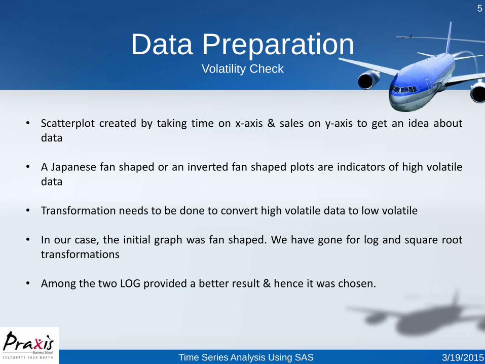
• Scatterplot created by taking time on x-axis & sales on y-axis to get an idea aboutdata

• A Japanese fan shaped or an inverted fan shaped plots are indicators of high volatiledata

• Transformation needs to be done to convert high volatile data to low volatile

• In our case, the initial graph was fan shaped. We have gone for log and square roottransformations

• Among the two LOG provided a better result & hence it was chosen.

Data PreparationVolatility Check

3/19/2015Time Series Analysis Using SAS

6

• A non stationary data is completely memory less with no fixed patterns.Such a datacan’t be used for forecasting

• Non-Stationarity is checked by using Augmented Dickey Fuller Test (ADF).

• Non-Stationarity can be removed by differencing

• In our case, data was found to be non-stationary

• Hence, differencing was done to make data stationary

Data PreparationNon-Stationarity Check

Note: Differencing was done on LOG transformed data

3/19/2015Time Series Analysis Using SAS

7

• Autocorrelation function(ACF) gives the correlation between Y(t) & Y(t-s); S is the period of lag

• If ACF gives high values at fixed interval, then it can be considered as period of seasonality

• A differencing of same order would be done to de-seasonalize the data

• In our case,it was found that ACF gave high values at fixed intervals of 12 (so, S=12)

• Hence differencing was done at an interval of 12

Data PreparationSeasonality Check

Creation of Test and Training Dataset

3/19/2015Time Series Analysis Using SAS

8

Training Dataset:Part of dataset which is used to build a model

Test Dataset:Part of dataset used to validate the model built

Forecasting needs to be done for 1 year(12 months), therefore we will keep last oneyear of data (year 1960) as the test dataset and rest of the data will be used to builtthe model as a training dataset.

Building Model and Validation

3/19/2015Time Series Analysis Using SAS

9

MINIC (Minimum Information Criteria) option under PROC ARIMA generates theminimum BIC (Bayesian Information Criteria) Model after exploring all the possiblecombinations of ‘p’ (Auto Regressive) and ‘q’ (Moving Average) lags from 0 to 5 (default).

3/19/2015Time Series Analysis Using SAS

10

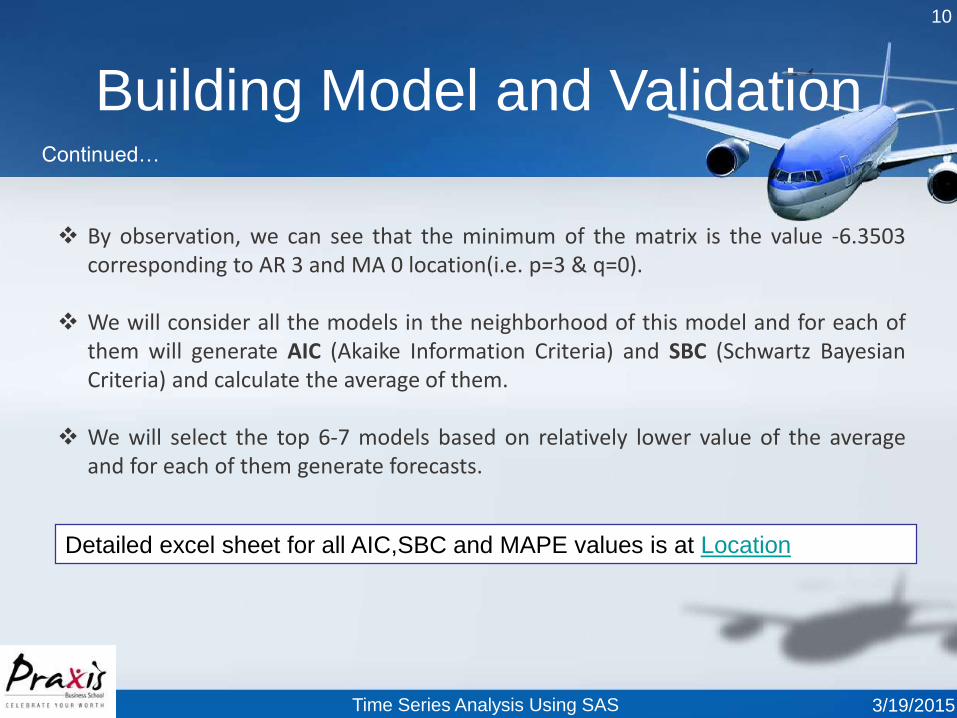
By observation, we can see that the minimum of the matrix is the value -6.3503corresponding to AR 3 and MA 0 location(i.e. p=3 & q=0).

We will consider all the models in the neighborhood of this model and for each ofthem will generate AIC (Akaike Information Criteria) and SBC (Schwartz BayesianCriteria) and calculate the average of them.

We will select the top 6-7 models based on relatively lower value of the averageand for each of them generate forecasts.

Detailed excel sheet for all AIC,SBC and MAPE values is at Location

Building Model and ValidationContinued…

Forecasting

3/19/2015Time Series Analysis Using SAS

11

The forecasts generated (for the year 1960) for each of the 6 combination selectedfrom AIC & SBC separately compared with the actual values of the same time pointstored in the test dataset

‘MAPE’ (Mean Absolute Percentage Error) is calculated for above 6 forecastedvalues for the year 1960

Lowest MAPE value comes out to be for P=0 and Q=3, hence final forecasting will bedone using this model.

Forecasted Values

3/19/2015Time Series Analysis Using SAS

12

Graphical Representation

3/19/2015Time Series Analysis Using SAS

13

50

100

150

200

250

300

350

400

450

500

550

600

650

700

Jan

-49

Ma

y-4

9

Se

p-4

9

Jan

-50

Ma

y-5

0

Se

p-5

0

Jan

-51

Ma

y-5

1

Se

p-5

1

Jan

-52

Ma

y-5

2

Se

p-5

2

Jan

-53

Ma

y-5

3

Se

p-5

3

Jan

-54

Ma

y-5

4

Se

p-5

4

Jan

-55

Ma

y-5

5

Se

p-5

5

Jan

-56

Ma

y-5

6

Se

p-5

6

Jan

-57

Ma

y-5

7

Se

p-5

7

Jan

-58

Ma

y-5

8

Se

p-5

8

Jan

-59

Ma

y-5

9

Se

p-5

9

Jan

-60

Ma

y-6

0

Se

p-6

0

Jan

-61

Ma

y-6

1

Se

p-6

1

Sa

les

Va

lue

s

Date

Actual Vs Forecast

Actual Sales Values Forecasted Sales Values

Appendix

3/19/2015Time Series Analysis Using SAS

14

Full Code is at “SAS code for forecasting”

15

3/19/2015Time Series Analysis Using SAS