THE USE OF EARNED VALUE IN FORCASTING … USE OF EARNED VALUE IN FORCASTING PROJECT DURATIONS Osama...
5
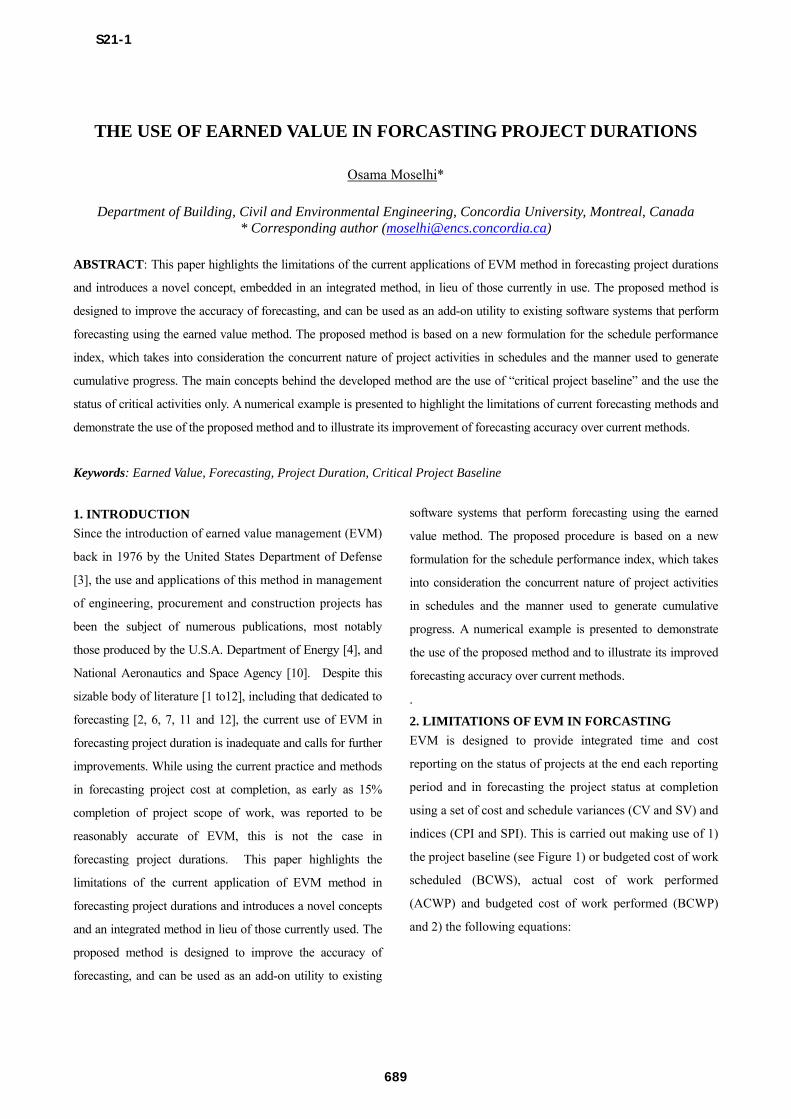
THE USE OF EARNED VALUE IN FORCASTING PROJECT DURATIONS Osama Moselhi * Department of Building, Civil and Environmental Engineering, Concordia University, Montreal, Canada * Corresponding author ([email protected] ) ABSTRACT: This paper highlights the limitations of the current applications of EVM method in forecasting project durations and introduces a novel concept, embedded in an integrated method, in lieu of those currently in use. The proposed method is designed to improve the accuracy of forecasting, and can be used as an add-on utility to existing software systems that perform forecasting using the earned value method. The proposed method is based on a new formulation for the schedule performance index, which takes into consideration the concurrent nature of project activities in schedules and the manner used to generate cumulative progress. The main concepts behind the developed method are the use of “critical project baseline” and the use the status of critical activities only. A numerical example is presented to highlight the limitations of current forecasting methods and demonstrate the use of the proposed method and to illustrate its improvement of forecasting accuracy over current methods. Keywords: Earned Value, Forecasting, Project Duration, Critical Project Baseline 1. INTRODUCTION Since the introduction of earned value management (EVM) back in 1976 by the United States Department of Defense [3], the use and applications of this method in management of engineering, procurement and construction projects has been the subject of numerous publications, most notably those produced by the U.S.A. Department of Energy [4], and National Aeronautics and Space Agency [10]. Despite this sizable body of literature [1 to12], including that dedicated to forecasting [2, 6, 7, 11 and 12], the current use of EVM in forecasting project duration is inadequate and calls for further improvements. While using the current practice and methods in forecasting project cost at completion, as early as 15% completion of project scope of work, was reported to be reasonably accurate of EVM, this is not the case in forecasting project durations. This paper highlights the limitations of the current application of EVM method in forecasting project durations and introduces a novel concepts and an integrated method in lieu of those currently used. The proposed method is designed to improve the accuracy of forecasting, and can be used as an add-on utility to existing software systems that perform forecasting using the earned value method. The proposed procedure is based on a new formulation for the schedule performance index, which takes into consideration the concurrent nature of project activities in schedules and the manner used to generate cumulative progress. A numerical example is presented to demonstrate the use of the proposed method and to illustrate its improved forecasting accuracy over current methods. . 2. LIMITATIONS OF EVM IN FORCASTING EVM is designed to provide integrated time and cost reporting on the status of projects at the end each reporting period and in forecasting the project status at completion using a set of cost and schedule variances (CV and SV) and indices (CPI and SPI). This is carried out making use of 1) the project baseline (see Figure 1) or budgeted cost of work scheduled (BCWS), actual cost of work performed (ACWP) and budgeted cost of work performed (BCWP) and 2) the following equations: S21-1 689
Transcript of THE USE OF EARNED VALUE IN FORCASTING … USE OF EARNED VALUE IN FORCASTING PROJECT DURATIONS Osama...
THE USE OF EARNED VALUE IN FORCASTING PROJECT DURATIONS
Osama Moselhi*
Department of Building, Civil and Environmental Engineering, Concordia University, Montreal, Canada
* Corresponding author ([email protected])
ABSTRACT: This paper highlights the limitations of the current applications of EVM method in forecasting project durations
and introduces a novel concept, embedded in an integrated method, in lieu of those currently in use. The proposed method is
designed to improve the accuracy of forecasting, and can be used as an add-on utility to existing software systems that perform
forecasting using the earned value method. The proposed method is based on a new formulation for the schedule performance
index, which takes into consideration the concurrent nature of project activities in schedules and the manner used to generate
cumulative progress. The main concepts behind the developed method are the use of “critical project baseline” and the use the
status of critical activities only. A numerical example is presented to highlight the limitations of current forecasting methods and
demonstrate the use of the proposed method and to illustrate its improvement of forecasting accuracy over current methods.
Keywords: Earned Value, Forecasting, Project Duration, Critical Project Baseline
1. INTRODUCTION
Since the introduction of earned value management (EVM)
back in 1976 by the United States Department of Defense
[3], the use and applications of this method in management
of engineering, procurement and construction projects has
been the subject of numerous publications, most notably
those produced by the U.S.A. Department of Energy [4], and
National Aeronautics and Space Agency [10]. Despite this
sizable body of literature [1 to12], including that dedicated to
forecasting [2, 6, 7, 11 and 12], the current use of EVM in
forecasting project duration is inadequate and calls for further
improvements. While using the current practice and methods
in forecasting project cost at completion, as early as 15%
completion of project scope of work, was reported to be
reasonably accurate of EVM, this is not the case in
forecasting project durations. This paper highlights the
limitations of the current application of EVM method in
forecasting project durations and introduces a novel concepts
and an integrated method in lieu of those currently used. The
proposed method is designed to improve the accuracy of
forecasting, and can be used as an add-on utility to existing
software systems that perform forecasting using the earned
value method. The proposed procedure is based on a new
formulation for the schedule performance index, which takes
into consideration the concurrent nature of project activities
in schedules and the manner used to generate cumulative
progress. A numerical example is presented to demonstrate
the use of the proposed method and to illustrate its improved
forecasting accuracy over current methods.
.
2. LIMITATIONS OF EVM IN FORCASTING
EVM is designed to provide integrated time and cost
reporting on the status of projects at the end each reporting
period and in forecasting the project status at completion
using a set of cost and schedule variances (CV and SV) and
indices (CPI and SPI). This is carried out making use of 1)
the project baseline (see Figure 1) or budgeted cost of work
scheduled (BCWS), actual cost of work performed
(ACWP) and budgeted cost of work performed (BCWP)
and 2) the following equations:
S21-1
689

Figure 1: EVM Parameters
CV = ACWP – BCWP ……………………………... (1)
SV = BCWP - BCWS………………………….……... (2)
CPI = BCWP/ACWP………………..………………... (3)
SPI = BCWP/BCWS………………….…..…………... (4)
While CV and CPI (Equations 1 and 3) represent
reasonably the cost status of a project, SV and SPI do not
equally represent its schedule status. Consider, for example,
a scenario where at the end of a reporting period it was
found that a number of critical activates are experiencing
considerable delays while non critical activities are way
ahead of planned progress such that the resulting SPI is
equal to1.0. Clearly such SPI erroneously indicates that the
project is on target schedule without any delay while in
actuality the project is behind schedule. In other words,
Equation 4 can mask the actual schedule performance as
the inclusion of noncritical activities could distort and
misrepresent the status of the project schedule.
In addition, while the above variances and indices provide
time and cost status reporting at the end of each reporting
period, forecasting the project status at completion in
current methods are based either on:
a) assuming the performance attained so far will
continue in the future all the way to project
completion, or
b) assuming that the project performance will be as
planned in the future all the way to project
completion
Accordingly, the forecasted project duration (Df) is
calculated respectively, based on its planned original
duration (Do) by:
Df = Do/SPI .....................................................................(5)
or
Df = Do + SVt …………………….……………………(6)
Others may ignore the application of EVM in such
forecasting and resort to updating/revising the project
schedule, focusing primarily on the remaining work to
completion. This, however, is costly and time consuming in
comparison to the direct application of EVM.
.
3. PROPSED METHOD
The proposed method considers:
(1) Critical activities to generate C-BCWS (critical project
baseline) and C-BCWP (earned value of critical activities)
to generate more realistic schedule variance (R-SV) and
schedule performance index (R-SPI) as follows:
R-SV = C-BCWP – C-WCWS ……….……………….. (7)
R-SPI = C-BCWP/ C-BCWS ……..……………………(8)
The time variance in units of time (SVt) is calculated as
depicted diagrammatically in Figure 1.
(2) The impact of performance unrepresentative periods,
which experienced unexpected weather conditions or
accidents, by either revising the performance or by
dropping such periods when generating the cumulative
performance.
(3) Incremental adaptive learning by forecasting C-BCWP
at the end of each remaining periods and comparing it with
actual when reaching that time. As such, adjustment factors
(AFs) at the end of each reporting period are generated:
AF = R-SPI actual/ R-SPI forecasted ……………..… (9)
The AF is then used to calculate adjusted R-SPI (A-R-SPI)
as:
A-R-SPI = AF * R-SPI .............................................. (10)
S21-1
690

The forecasted project duration (Df) is then calculated as:
Df = Do / (A-R-SPI) ..................................................... (11)
or
Df = Do + SVt ……………...……………………. .. (12)
or
Df = De + SVt + (Do- De) / (A-R-SPI)......................... (13)
In which De is the elapsed duration
4. NUMERICAL EXAMPLE
The PDM network of this project example is shown in
Figure 1. The project has duration of 8 month and the latest
progress period is at half way of its planned original
duration. This example is used here to highlight the
limitations of current methods, to demonstrate the use of
the proposed method and to illustrate its improvement in
the accuracy of forecasting project duration at completion.
The data used in the analysis is included in Table 1.
Fig.1 PDM Diagram
Table 1 Activities durations and direct cost
Act
ivit
y
Du
rati
on
ES
EF
LS
LF
TF
Tot
al
Dir
ect
Cos
t D
irec
t
Cos
t /
Mon
th
A 1 0 1 0 1 0 $1,000 $1,000
B 3 0 3 2 5 2 $12,000 $4,000
C 1 1 2 4 5 3 $4,000 $4,000
D 6 1 7 1 7 0 $6,000 $1,000
E 2 3 5 5 7 2 $16,000 $8,000
F 1 7 8 7 8 0 $1,000 $1,000
The project baseline under three different scenarios was
generated as shown in Table 2 and in Figure 2. The
cumulative progress at the end of month 4 was calculated
as shown in Table 3.
Table 2: Project baseline (BCWS)
Early start Late start Critical Activities
Tim
e (m
onth
)
Per
iod
BC
WS
(E
S)*
Per
iod
BC
WS
(L
S)*
Per
iod
BC
WS
(C
ri.)
*
1 5 5 1 1 1 1
2 11 16 3 4 3 4
3 7 23 7 11 3 7
4 11 34 7 18 3 1
5 11 45 11 29 3 13
6 3 48 11 4 3 16
7 3 51 11 51 3 19
8 1 52 1 52 1 20
*Cost is in thousands of dollars
Fig. 2 Project baseline (BCWS)
The earned value analyses were performed using current
methods, i.e. Equations 1 to 6, and the proposed method as
described in Section 3 above. Three scenarios were
considered; 1) current EVM methods based on early start
S21-1
691
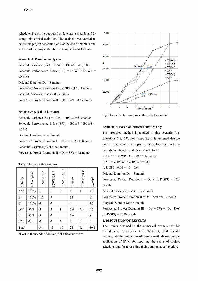
schedule, 2) as in 1) but based on late start schedule and 3)
using only critical activities. The analysis was carried to
determine project schedule status at the end of month 4 and
to forecast the project duration at completion as follows:
Scenario-1: Based on early start
Schedule Variance (SV) = BCWP − BCWS= -$6,000.0
Schedule Performance Index (SPI) = BCWP / BCWS =
0.82352
Original Duration Do = 8 month
Forecasted Project Duration-I = Do/SPI = 9.7142 month
Schedule Variance (SVt) = 0.55 month
Forecasted Project Duration-II = Do + SVt = 8.55 month
Senario-2: Based on late start
Schedule Variance (SV) = BCWP − BCWS= $10,000.0
Schedule Performance Index (SPI) = BCWP / BCWS =
1.5556
Original Duration Do = 8 month
Forecasted Project Duration-I = Do / SPI = 5.1428month
Schedule Variance (SVt) = -0.9 month
Forecasted Project Duration-II = Do + SVt = 7.1 month
Table 3 Earned value analysis
Act
ivity
% C
ompl
ete
BC
WS
(ES
)*
BC
WS
(LS
)*
BC
WS
(C
ri.)
*
BC
WP
*
BC
WP
(cr
i.)*
AC
WP
*
A** 100% 1 1 1 1 1 1.1
B 100% 1.2 8 12 11
C 100% 4 0 4 3.5
D** 30% 9 9 9 5.4 5.4 6.5
E 35% 8 0 5.6 8
F** 0% 0 0 0 0 0 0
Total 34 18 10 28 6.4 30.1
*Cost in thousands of dollars, **Critical activities
Fig.3 Earned value analysis at the end of month 4
Scenario-3: Based on critical activities only
The proposed method is applied in this scenario (i.e.
Equations 7 to 13). For simplicity it is assumed that no
unusual incidents have impacted the performance in the 4
periods and therefore AF is set equals to 1.0.
R-SV = C-BCWP − C-BCWS= -$3,600.0
R-SPI = C-BCWP / C-BCWS = 0.64
A-R-SPI = 0.64 x 1.0 = 0.64
Original Duration Do = 8 month
Forecasted Project Duration-I = Do / (A-R-SPI) = 12.5
month
Schedule Variance (SVt) = 1.25 month
Forecasted Project Duration-II = Do + SVt = 9.25 month
Elapsed Duration De = 4 month
Forecasted Project Duration-III = De + SVt + (Do- De)/
(A-R-SPI) = 11.50 month
5. DISCUSSION OF RESULTS
The results obtained in the numerical example exhibit
considerable differences (see Table 4) and clearly
demonstrate the limitations of current methods used in the
application of EVM for reporting the status of project
schedules and for forecasting their duration at completion.
S21-1
692

Table 4 Forecasted project durations (month)
D
ura
tion
Sce
nar
io 1
Sce
nar
io 2
Ave
rage
1&
2
Sce
nar
io 3
I 9.71 5.14 7.42 12.50
II 8.55 7.10 7.82 9.25
III --- --- 11.50
Clearly the differences between scenarios 1 and 2 may not
be encountered in practice as the schedule will be that
approved by the owner and/or its agent and it commonly
leans toward early start schedule. It is included in this
example to demonstrate its impact on earned value analysis.
It is important here to compare scenario 1, or the average
of scenarios 1 and 2, to scenario 3. We see in this example
how current methods (used in scenarios 1 and 2)
underestimate the forecasted project duration at completion.
6. SUMMARY AND CONCLUDING REMARKS
The use the two the widely used two methods, described
above in Section 2, for forecasting may produce to
inaccurate results, which leads to unrealistic forecasting of
the project status at completion. This is of considerable
importance, particularly in forecasting project durations. In
this case it is recommended to use only critical activities in
generating project baseline and subsequently in generating
schedule variances and indices as outlined in the proposed
method. The results obtained from the numerical example
demonstrate how erroneous forecasting project duration
can be when applying the current EVM methods.
ACKNOWLEDGMENTS
The author would like to thanks Mr. Ali Montaser for his
assistance in generating the results of the numerical
example and the preparation of its related tables and
figures.
REFERENCES
[1] Alshibani, A., “A computerized cost and schedule
control system for construction projects”, Master’s thesis,
Civil, Building, and Environmental Engineering,
Concordia University, Montreal, Canada, 1999.
[2] Christensen, D.S, Antolini, R.C. and Mckinney, J.W.,
“A review of EAC Research”, Journal of Cost Analysis and
Management, Spring Issue, pp. 41-62, 1995.
[3] Department of Defense, 1967. Performance
Measurement for Selected Acquisitions, DODI 7000.2.
[4] Department of Energy, 1980. Cost/Schedule Control
Systems Criteria for Contract Performance Measurement:
Implementation Guide, DOE/CR-0015, Office of the
Controller.
[5] Fleming, Q. W. and Koppelman, J.M., Earned Value
Project Management, 3rd Ed., Newton Square, Pa., USA:
Project Management Institute, 2005.
[6] Hassanein A., and Moselhi O., “Tracking and Control
of Linear Infrastructure Projects”, 5th Construction
Specialty Conference of the Canadian Society for Civil
Engineering, Moncton, Nouveau-Brunswick, Canada, 2003.
[7] Ji, Li. “Web-based integrated project control”, PhD’s
thesis, Civil, Building, and Environmental Engineering,
Concordia University, Montreal, Canada, 2004.
[8] Moselhi, O.,. Applied Earned Value for Project Control,
proc. of the CIB W-65 7th International Symposium on
Organization and Management of Construction, Port of Spain,
Trinidad. 1993
[9] Moselhi, O., Ji,li, and Alkass, Sabah,“Web-based
integrated project control System.” Construction
Management and Economics. Vol. 1, pp. 35-46, 2004.
[10] NASA, “Integrated Baseline Review (IBR) Handbook,
SP-2010-3406.
[11] Paul Teicholz, “Forecasting final cost and budget of
construction projects”, Journal of Computing in Civil
Engineering, Vol. 7, No. 4, October, 1993.
[12] Xiao hui, Xiao, “Trending and forecasting in
construction operations”, Master’s thesis, Civil, Building,
and Environmental Engineering, Concordia University,
Montreal, Canada. 2009.
S21-1
693