College of the Holy CrossCrossWorks

Honors Theses Honors Projects

2009

The Use of a Lock-In Amplifier to Stabilize theFrequency of a Laser DiodeJose M. JuarezCollege of the Holy Cross, jose.miguel.juarez87@gmail.com

Follow this and additional works at: https://crossworks.holycross.edu/honors

Part of the Atomic, Molecular and Optical Physics Commons

This Thesis is brought to you for free and open access by the Honors Projects at CrossWorks. It has been accepted for inclusion in Honors Theses by anauthorized administrator of CrossWorks.

Recommended CitationJuarez, Jose M., "The Use of a Lock-In Amplifier to Stabilize the Frequency of a Laser Diode" (2009). Honors Theses. 9.https://crossworks.holycross.edu/honors/9

The Use of a Lock-In Amplifier to Stabilize the Frequency of a Diode Laser

Miguel Juarez ‘09 and Professor Paul Oxley

Department of Physics College of the Holy Cross

Acknowledgements

We would like to express our appreciation to our readers, Professor Timothy Roach and

Professor Robert Garvey, for their time and valuable contributions to this thesis. We would also

like to thank Professor Roach for his generosity in allowing us to work in his lab and for

allowing us to use some pieces of his laboratory equipment. Without these contributions this

thesis would not have been possible.

We also owe thanks to Professor Janine Shertzer for contributing to the editing of this

thesis and to Professor De-Ping Yang for his invaluable assistance in the construction of our

lock-in amplifier. We are very grateful for the help that we have received from Dick Miller, the

college machinist, in constructing some of the parts for our laser. Also, we thank Diane Jepson,

the Physics Department Administrative Assistant, for helping us with ordering the parts for our

experiment.

We are especially grateful to the Richard B. Fisher Summer Student Research Fellowship

Fund, the Research Corporation, the College Honors Program, the Summer Research Program,

and the Physics Department for their generous support.

Abstract

We have designed, constructed, and tested a lock-in amplifier with readily available electronic

components and homebuilt analog circuits. Its performance is comparable to that of a

commercial unit, but it costs significantly less and is much more compact. The various

components of our lock-in amplifier are discussed and the basic principles behind the function

and operation of this versatile device are explained. We have also assembled a laser system and

used the output signal of our lock-in amplifier in a negative feedback loop to stabilize the

frequency of our laser to an atomic reference frequency.

Contents 1 Introduction 1

1.1 The Laser …………………………………………………………………………...……. 1

1.2 Our Lock-In Amplifier ...………………………………………………………………… 2

1.3 Our Laser Setup …………………………………………………………………………. 2

1.4 Stabilizing the Frequency of Our Laser ………………………….……………………… 3

1.5 Project Overview ………………………………………………………………………... 5

2 Our Lock-In Amplifier 7

2.1 Introduction …………………………………………………………………………....… 7

2.2 Dither and Input Signals ………………………………….……………………………... 8

2.3 Differential AC Amplifier ……………………………...………………………………... 8

2.4 Phase Shifter ………………………...………………………………………………….. 10

2.5 Mixer ………….……………………………………..…………………………………. 14

2.6 Low-Pass Filter ……………………...……………………………..…………………… 16

2.7 DC Amplifier ……………………...……………………………..………………...…… 18

3 Our Laser Setup and Frequency Tuning Parameters 23

3.1 Introduction …………………………………………………………………………….. 23

3.2 The Laser Diode ……………………………………………………….……………….. 24

3.3 Our Mechanical Setup ……………………………………………...………………….. 26

3.4 First Tuning Parameter: Laser Temperature …………………………………………… 27

3.5 Second Tuning Parameter: Injection Current ……………………………….…………. 27

3.6 Third Tuning Parameter: Grating Optical Feedback …………………………………... 28

3.7 Closing Remarks …………………………………………………………………..….... 30

4 Our Optical Setup and Saturated Absorption Spectroscopy 31

4.1 Introduction …………………………………………………………………………….. 31

4.2 Monitoring the Laser Frequency ……………………………………………………….. 33

4.3 Rubidium Vapor Cell …………………………………………………………………... 35

4.4 Doppler-Broadened Absorption Spectrum ……………………………………….…….. 36

4.5 Probe and Pump Beams ……………………………………………………….……….. 38

4.6 Saturated Absorption Spectroscopy ................................................................................. 39

4.7 Improving the Saturated Absorption Signal ………………………………………......... 41

4.8 Closing Remarks ……………………………………………………………………….. 42

5 Stabilizing the Frequency of Our Laser 43

5.1 Introduction …………………………………………………………………………..… 43

5.2 Dither and Input Signals ………………………………………….…………………….. 43

5.3 The Error Signal ……………………………………………….……………………….. 44

5.4 Stabilizing the Frequency of Our Laser …………………………….………………..… 49

A Conclusion 51

B References 52

1

Chapter 1

Introduction

1.1 The Laser

The laser is an extremely useful device that is utilized in a wide variety of scientific, industrial,

commercial, and medical applications. In a remarkably short report of only two pages, the first

working laser was introduced by Theodore Maiman on 16 May 1960 at the Hughes Research

Laboratory in California [1]. Since then, the laser has not only created a multi-billion dollar

industry, but it has also revolutionized science and technology in countless and significant ways

[2]. For instance, today the laser is being used to investigate the properties of atoms to an

unprecedented level of precision. Lasers are integral components of the technology used in nano-

and atomic-scale length metrology, optical communications, and precision spectroscopy, all

cutting-edge areas of research in physics [3].

Dramatic new developments have been made and are still being made using lasers, such

as their use in slowing down atoms to extraordinarily low temperatures that have never before

been achieved. This new level of control of atomic motion is allowing researchers today to better

observe and understand the behavior of atoms [4]. However, such applications are only possible

with a laser which emits light with a single, exceptionally stable frequency. In this thesis, we

show how this precise level of frequency stability can be attained using a lock-in amplifier and a

fixed reference frequency against which the laser frequency can be stabilized.

2

1.2 Our Lock-In Amplifier

A lock-in amplifier is a very sensitive electronic device used to detect, isolate, and amplify very

small AC signals that may be buried in substantial amounts of unwanted noise. The lock-in

amplifier is extremely versatile and is used in many fields of physics, including atomic physics.

For instance, in solid-states physics, it is used to measure the temperature dependence of the

resistance of metals and superconductors, study the Hall Effect in semiconductors, and detect

small temperature changes by means of a thermistor bridge [5]. The lock-in technique is also

used in some astrophysical experiments involving the measurement of cosmic radiation [6].

In this thesis, we describe the construction of a lock-in amplifier using readily available

electronic components. Our lock-in amplifier consists of five different types of circuits, which

we have designed and built. They include the following: a differential AC amplifier, a phase

shifter, a mixer, a low-pass filter, and a DC amplifier. These circuit components have been tested

both individually and collectively, and they have met our design goals. In our experiment, our

lock-in amplifier is used to detect a laser frequency change and produce a signal voltage which

can be fed back to our laser to correct this change, thereby stabilizing the laser frequency.

1.3 Our Laser Setup

In our experiment, we wish to stabilize the frequency of a diode laser. In comparison to many

other laser sources, the output power of a diode laser is very stable, allowing for easier

measurements of absorption or fluorescence [7]. These lasers are also inexpensive, very

compact, and available in many wavelengths which can be tuned over a few nanometers.

Diode lasers emit light over a narrow range of frequencies. However, the laser

frequency varies with small fluctuations in the laser current and temperature. These fluctuations

3

are undesirable in precision experiments. By stabilizing the laser frequency to a stable external

optical reference, it is possible to narrow the range of wavelengths that are emitted by the laser

over time [8]. For a reference frequency, we use a specific atomic transition. The frequency of

light needed to excite such a transition is fixed by the atomic properties of the reference gas and

is therefore very stable.

A diffraction grating is included in our laser setup to allow us to control the frequency

of our laser. The grating allows for passive stabilization as well as external control. When the

output beam of the laser strikes the grating, the first-order diffracted beam is directed back into

the laser, providing frequency-selective optical feedback [9]. This feedback keeps the laser

producing light at the same frequency as that of the optical feedback. Different lasing

frequencies may therefore be selected by adjusting the grating angle. This control allows us to

keep the laser frequency the same as the frequency of the external reference.

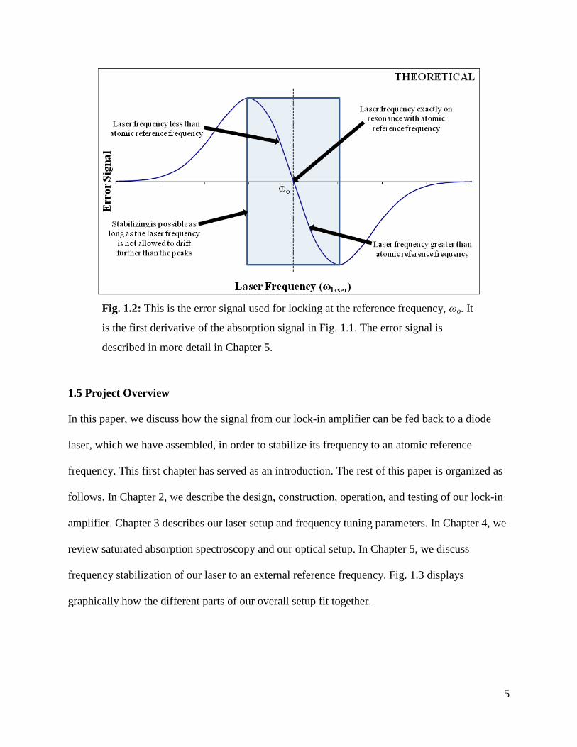
1.4 Stabilizing the Frequency of Our Laser

We wish to generate a control signal, commonly called an error signal, that we can use to

stabilize the frequency of our laser. In order to do this, we impose a dither (a small modulation)

on the laser frequency by repeatedly changing the grating angle back and forth at ωd. An

absorption signal is acquired by measuring the laser light passing through the atomic reference

gas with transition frequency ωo. The absorption signal is fed into our lock-in amplifier, which

provides an output signal that is directly proportional to the amount of 1ωd (dither frequency)

signal present in the absorption signal, while ignoring all other frequency components. The

output signal of our lock-in amplifier serves as an error signal that is proportional to the first

derivative of the absorption signal. Therefore, when the laser frequency ωlaser exactly matches

4

the external reference frequency ωo, no error signal is generated [10]. However, a drift towards

higher or lower laser frequency results in an error signal that is directly proportional to the

amount of frequency drift. The error signal therefore provides a continuous restoring signal that

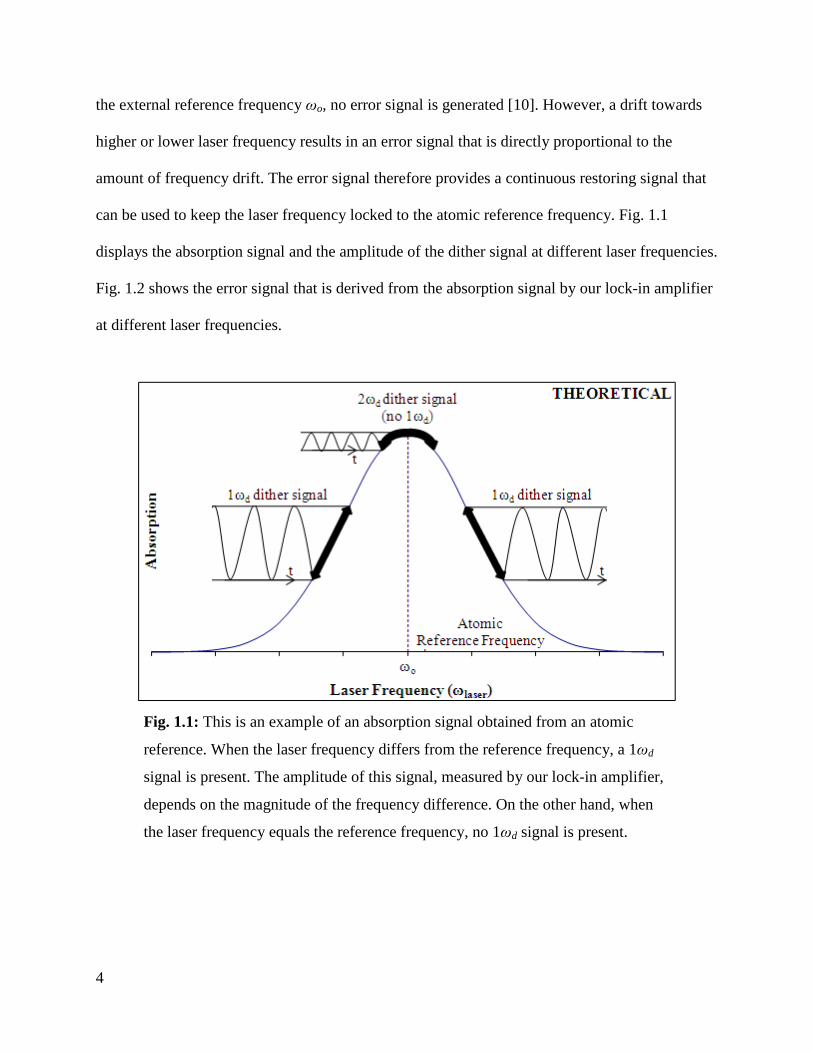
can be used to keep the laser frequency locked to the atomic reference frequency. Fig. 1.1

displays the absorption signal and the amplitude of the dither signal at different laser frequencies.

Fig. 1.2 shows the error signal that is derived from the absorption signal by our lock-in amplifier

at different laser frequencies.

Fig. 1.1: This is an example of an absorption signal obtained from an atomic

reference. When the laser frequency differs from the reference frequency, a 1ωd

signal is present. The amplitude of this signal, measured by our lock-in amplifier,

depends on the magnitude of the frequency difference. On the other hand, when

the laser frequency equals the reference frequency, no 1ωd signal is present.

5

Fig. 1.2: This is the error signal used for locking at the reference frequency, ωo. It

is the first derivative of the absorption signal in Fig. 1.1. The error signal is

described in more detail in Chapter 5.

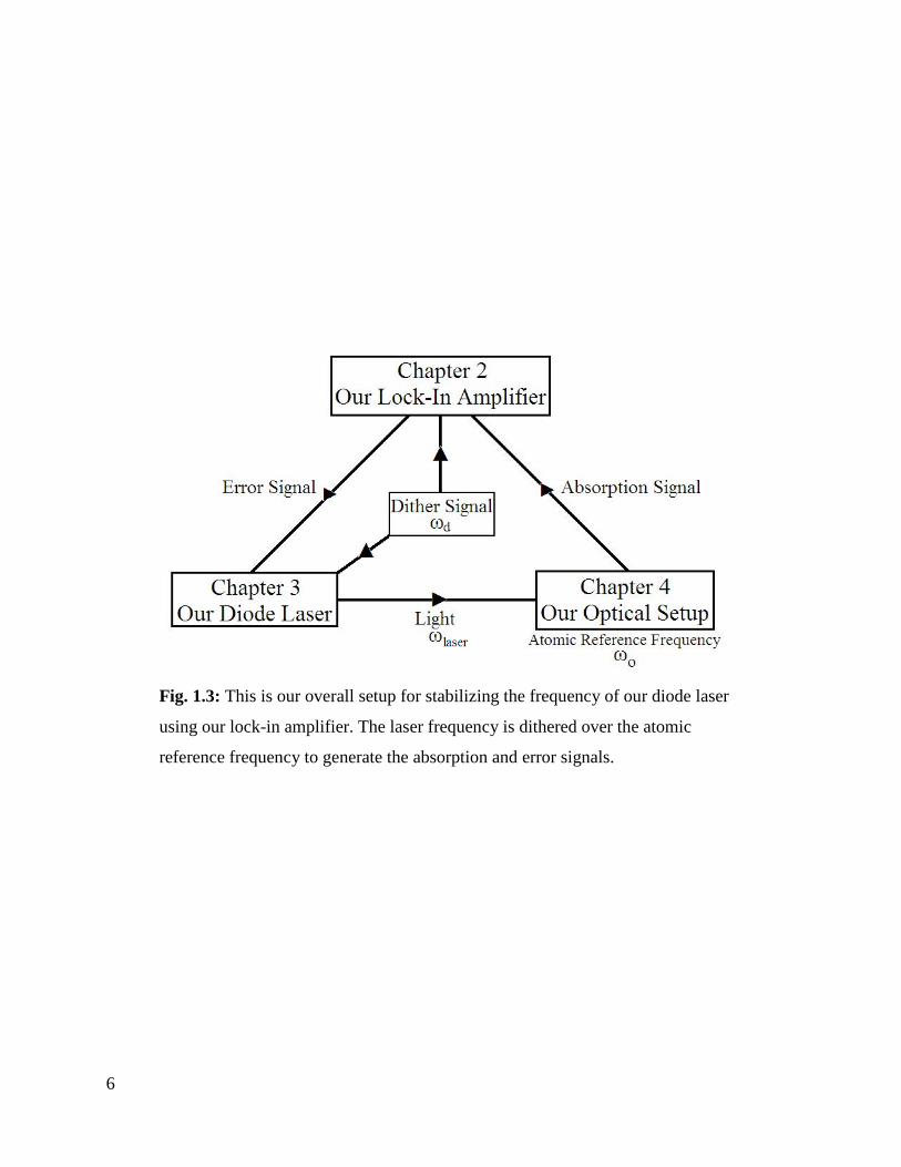
1.5 Project Overview

In this paper, we discuss how the signal from our lock-in amplifier can be fed back to a diode

laser, which we have assembled, in order to stabilize its frequency to an atomic reference

frequency. This first chapter has served as an introduction. The rest of this paper is organized as

follows. In Chapter 2, we describe the design, construction, operation, and testing of our lock-in

amplifier. Chapter 3 describes our laser setup and frequency tuning parameters. In Chapter 4, we

review saturated absorption spectroscopy and our optical setup. In Chapter 5, we discuss

frequency stabilization of our laser to an external reference frequency. Fig. 1.3 displays

graphically how the different parts of our overall setup fit together.

6

Fig. 1.3: This is our overall setup for stabilizing the frequency of our diode laser

using our lock-in amplifier. The laser frequency is dithered over the atomic

reference frequency to generate the absorption and error signals.

7

Chapter 2

Our Lock-In Amplifier

2.1 Introduction

The lock-in amplifier is an extremely useful device with applications in many scientific

disciplines. For instance, in spectroscopy and studies of fluorescence and luminescence, it is used

to recover very small optical signals. In electronics and cryogenics, the lock-in amplifier can be

used in component characterization, bridge networks, and measurements of the resistance of

superconductors. This versatile device can also be used as an AC signal recovery instrument, a

vector voltmeter, a phase meter, a spectrum analyzer, and a noise measurement unit. Evidently,

the lock-in amplifier is an invaluable addition to any physics laboratory.

As noted in Chapter 1, the purpose of our lock-in amplifier is to provide a DC output

voltage, the “error signal,” proportional to the amount of 1ωd signal present in the lock-in input

signal. In this chapter we describe how this is accomplished with our lock-in amplifier.

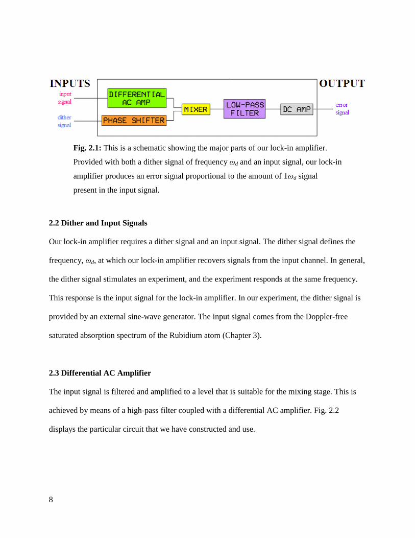
Our lock-in amplifier is based on a design by M. Weel and A. Kumarakrishnan [10]. It is

composed of five major parts: a differential AC amplifier, a phase shifter, a mixer, a low-pass

filter, and a DC amplifier. Fig. 2.1 displays the overall setup of our lock-in amplifier, which is

discussed in this chapter.

8

Fig. 2.1: This is a schematic showing the major parts of our lock-in amplifier.

Provided with both a dither signal of frequency ωd and an input signal, our lock-in

amplifier produces an error signal proportional to the amount of 1ωd signal

present in the input signal.

2.2 Dither and Input Signals

Our lock-in amplifier requires a dither signal and an input signal. The dither signal defines the

frequency, ωd, at which our lock-in amplifier recovers signals from the input channel. In general,

the dither signal stimulates an experiment, and the experiment responds at the same frequency.

This response is the input signal for the lock-in amplifier. In our experiment, the dither signal is

provided by an external sine-wave generator. The input signal comes from the Doppler-free

saturated absorption spectrum of the Rubidium atom (Chapter 3).

2.3 Differential AC Amplifier

The input signal is filtered and amplified to a level that is suitable for the mixing stage. This is

achieved by means of a high-pass filter coupled with a differential AC amplifier. Fig. 2.2

displays the particular circuit that we have constructed and use.

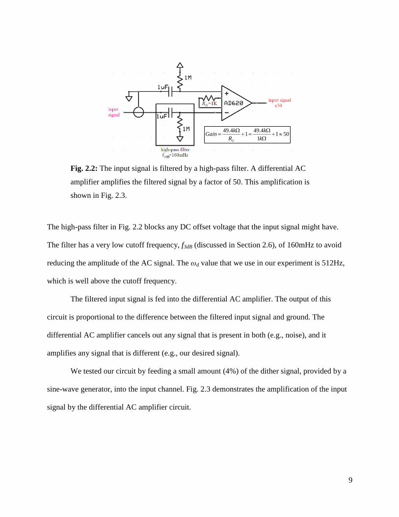
9

Fig. 2.2: The input signal is filtered by a high-pass filter. A differential AC

amplifier amplifies the filtered signal by a factor of 50. This amplification is

shown in Fig. 2.3.

The high-pass filter in Fig. 2.2 blocks any DC offset voltage that the input signal might have.

The filter has a very low cutoff frequency, f3dB (discussed in Section 2.6), of 160mHz to avoid

reducing the amplitude of the AC signal. The ωd value that we use in our experiment is 512Hz,

which is well above the cutoff frequency.

The filtered input signal is fed into the differential AC amplifier. The output of this

circuit is proportional to the difference between the filtered input signal and ground. The

differential AC amplifier cancels out any signal that is present in both (e.g., noise), and it

amplifies any signal that is different (e.g., our desired signal).

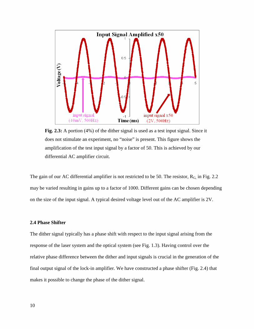
We tested our circuit by feeding a small amount (4%) of the dither signal, provided by a

sine-wave generator, into the input channel. Fig. 2.3 demonstrates the amplification of the input

signal by the differential AC amplifier circuit.

5011

4.4914.49≈+

ΩΩ

=+Ω

=k

kR

kGainG

10

Fig. 2.3: A portion (4%) of the dither signal is used as a test input signal. Since it

does not stimulate an experiment, no “noise” is present. This figure shows the

amplification of the test input signal by a factor of 50. This is achieved by our

differential AC amplifier circuit.

The gain of our AC differential amplifier is not restricted to be 50. The resistor, RG, in Fig. 2.2

may be varied resulting in gains up to a factor of 1000. Different gains can be chosen depending

on the size of the input signal. A typical desired voltage level out of the AC amplifier is 2V.

2.4 Phase Shifter

The dither signal typically has a phase shift with respect to the input signal arising from the

response of the laser system and the optical system (see Fig. 1.3). Having control over the

relative phase difference between the dither and input signals is crucial in the generation of the

final output signal of the lock-in amplifier. We have constructed a phase shifter (Fig. 2.4) that

makes it possible to change the phase of the dither signal.

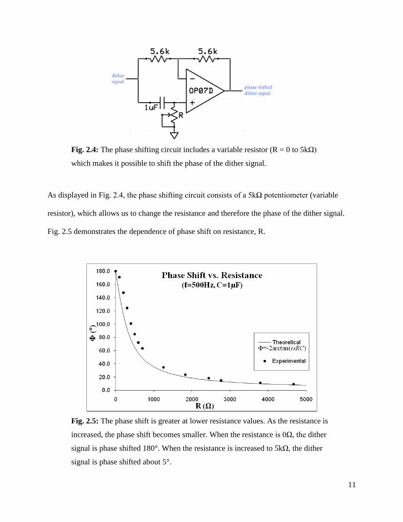
11

Fig. 2.4: The phase shifting circuit includes a variable resistor (R = 0 to 5kΩ)

which makes it possible to shift the phase of the dither signal.

As displayed in Fig. 2.4, the phase shifting circuit consists of a 5kΩ potentiometer (variable

resistor), which allows us to change the resistance and therefore the phase of the dither signal.

Fig. 2.5 demonstrates the dependence of phase shift on resistance, R.

Fig. 2.5: The phase shift is greater at lower resistance values. As the resistance is

increased, the phase shift becomes smaller. When the resistance is 0Ω, the dither

signal is phase shifted 180°. When the resistance is increased to 5kΩ, the dither

signal is phase shifted about 5°.

12

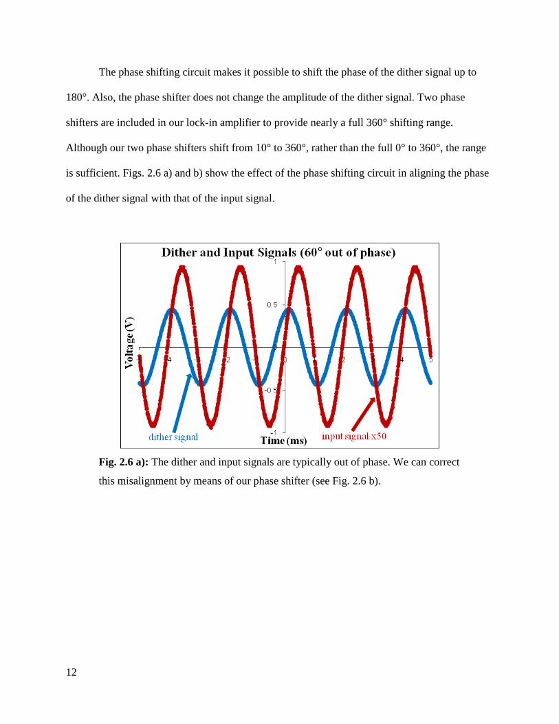
The phase shifting circuit makes it possible to shift the phase of the dither signal up to

180°. Also, the phase shifter does not change the amplitude of the dither signal. Two phase

shifters are included in our lock-in amplifier to provide nearly a full 360° shifting range.

Although our two phase shifters shift from 10° to 360°, rather than the full 0° to 360°, the range

is sufficient. Figs. 2.6 a) and b) show the effect of the phase shifting circuit in aligning the phase

of the dither signal with that of the input signal.

Fig. 2.6 a): The dither and input signals are typically out of phase. We can correct

this misalignment by means of our phase shifter (see Fig. 2.6 b).

13

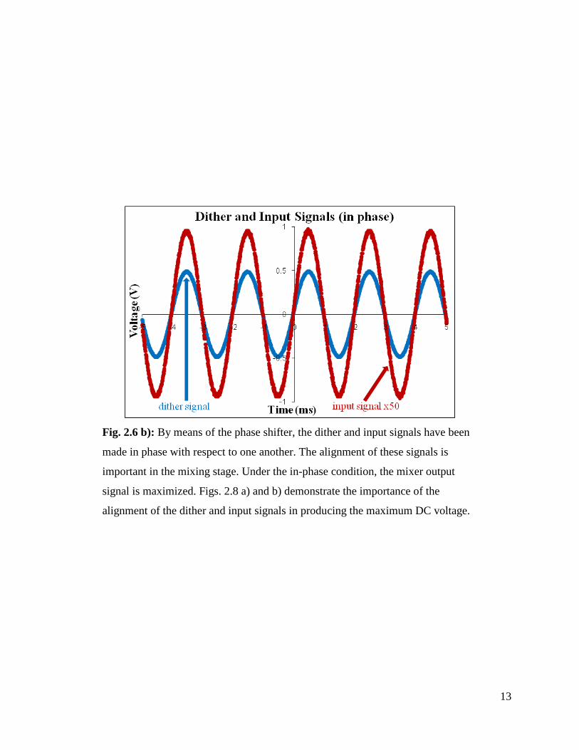
Fig. 2.6 b): By means of the phase shifter, the dither and input signals have been

made in phase with respect to one another. The alignment of these signals is

important in the mixing stage. Under the in-phase condition, the mixer output

signal is maximized. Figs. 2.8 a) and b) demonstrate the importance of the

alignment of the dither and input signals in producing the maximum DC voltage.

14

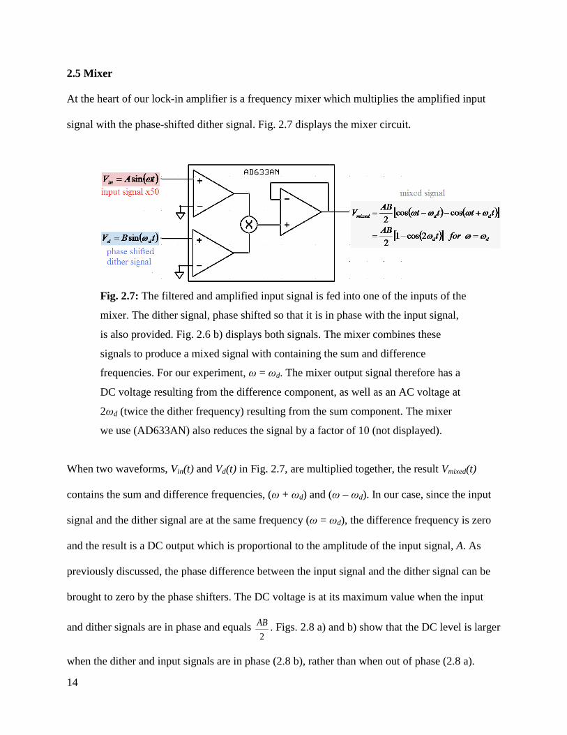
2.5 Mixer

At the heart of our lock-in amplifier is a frequency mixer which multiplies the amplified input

signal with the phase-shifted dither signal. Fig. 2.7 displays the mixer circuit.

Fig. 2.7: The filtered and amplified input signal is fed into one of the inputs of the

mixer. The dither signal, phase shifted so that it is in phase with the input signal,

is also provided. Fig. 2.6 b) displays both signals. The mixer combines these

signals to produce a mixed signal with containing the sum and difference

frequencies. For our experiment, ω = ωd. The mixer output signal therefore has a

DC voltage resulting from the difference component, as well as an AC voltage at

2ωd (twice the dither frequency) resulting from the sum component. The mixer

we use (AD633AN) also reduces the signal by a factor of 10 (not displayed).

When two waveforms, Vin(t) and Vd(t) in Fig. 2.7, are multiplied together, the result Vmixed(t)

contains the sum and difference frequencies, (ω + ωd) and (ω – ωd). In our case, since the input

signal and the dither signal are at the same frequency (ω = ωd), the difference frequency is zero

and the result is a DC output which is proportional to the amplitude of the input signal, A. As

previously discussed, the phase difference between the input signal and the dither signal can be

brought to zero by the phase shifters. The DC voltage is at its maximum value when the input

and dither signals are in phase and equals 2

AB . Figs. 2.8 a) and b) show that the DC level is larger

when the dither and input signals are in phase (2.8 b), rather than when out of phase (2.8 a).

15

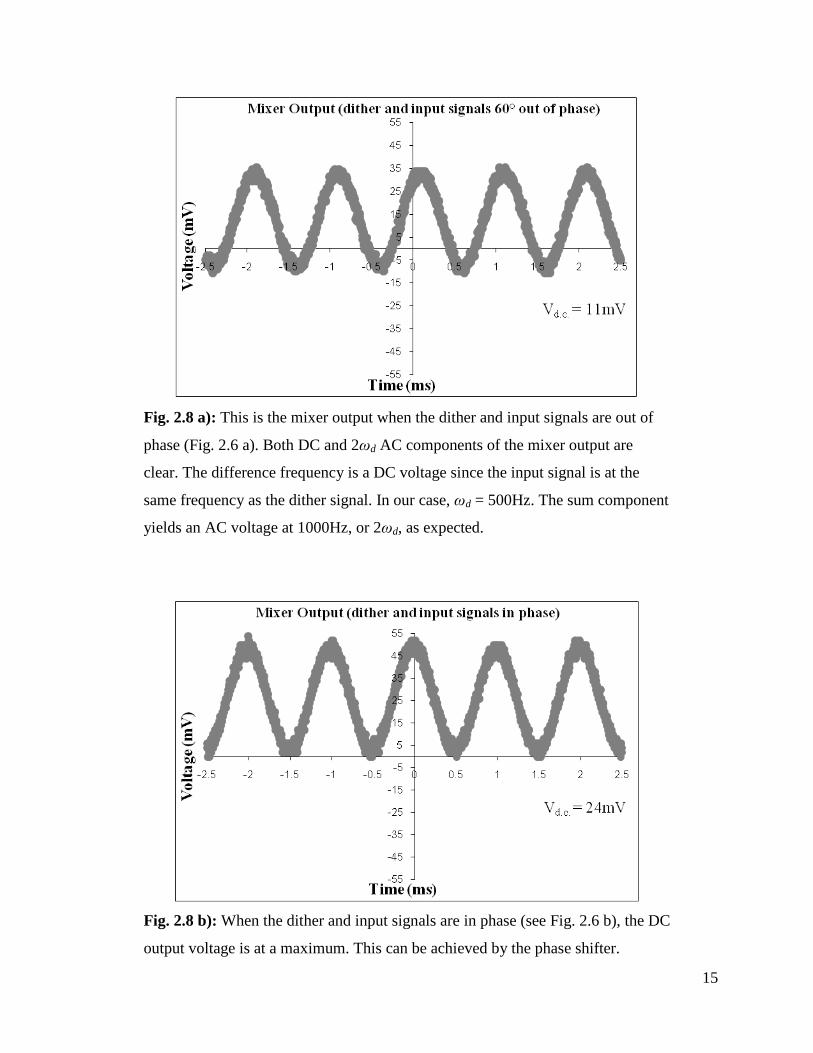
Fig. 2.8 a): This is the mixer output when the dither and input signals are out of

phase (Fig. 2.6 a). Both DC and 2ωd AC components of the mixer output are

clear. The difference frequency is a DC voltage since the input signal is at the

same frequency as the dither signal. In our case, ωd = 500Hz. The sum component

yields an AC voltage at 1000Hz, or 2ωd, as expected.

Fig. 2.8 b): When the dither and input signals are in phase (see Fig. 2.6 b), the DC

output voltage is at a maximum. This can be achieved by the phase shifter.

16

As indicated in Figs. 2.8 a) and b), in addition to the DC component another component at twice

the frequency of the dither signal (2ωd) results from the mixing. This is the sum frequency. This

component is eliminated so that the output of our lock-in amplifier is only the DC voltage.

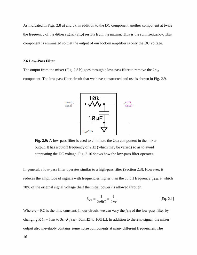
2.6 Low-Pass Filter

The output from the mixer (Fig. 2.8 b) goes through a low-pass filter to remove the 2ωd

component. The low-pass filter circuit that we have constructed and use is shown in Fig. 2.9.

Fig. 2.9: A low-pass filter is used to eliminate the 2ωd component in the mixer

output. It has a cutoff frequency of 2Hz (which may be varied) so as to avoid

attenuating the DC voltage. Fig. 2.10 shows how the low-pass filter operates.

In general, a low-pass filter operates similar to a high-pass filter (Section 2.3). However, it

reduces the amplitude of signals with frequencies higher than the cutoff frequency, f3dB, at which

70% of the original signal voltage (half the initial power) is allowed through.

πτπ 21

21

3 ==RC

f dB [Eq. 2.1]

Where τ = RC is the time constant. In our circuit, we can vary the f3dB of the low-pass filter by

changing R (τ = 1ms to 3s f3dB = 50mHZ to 160Hz). In addition to the 2ωd signal, the mixer

output also inevitably contains some noise components at many different frequencies. The

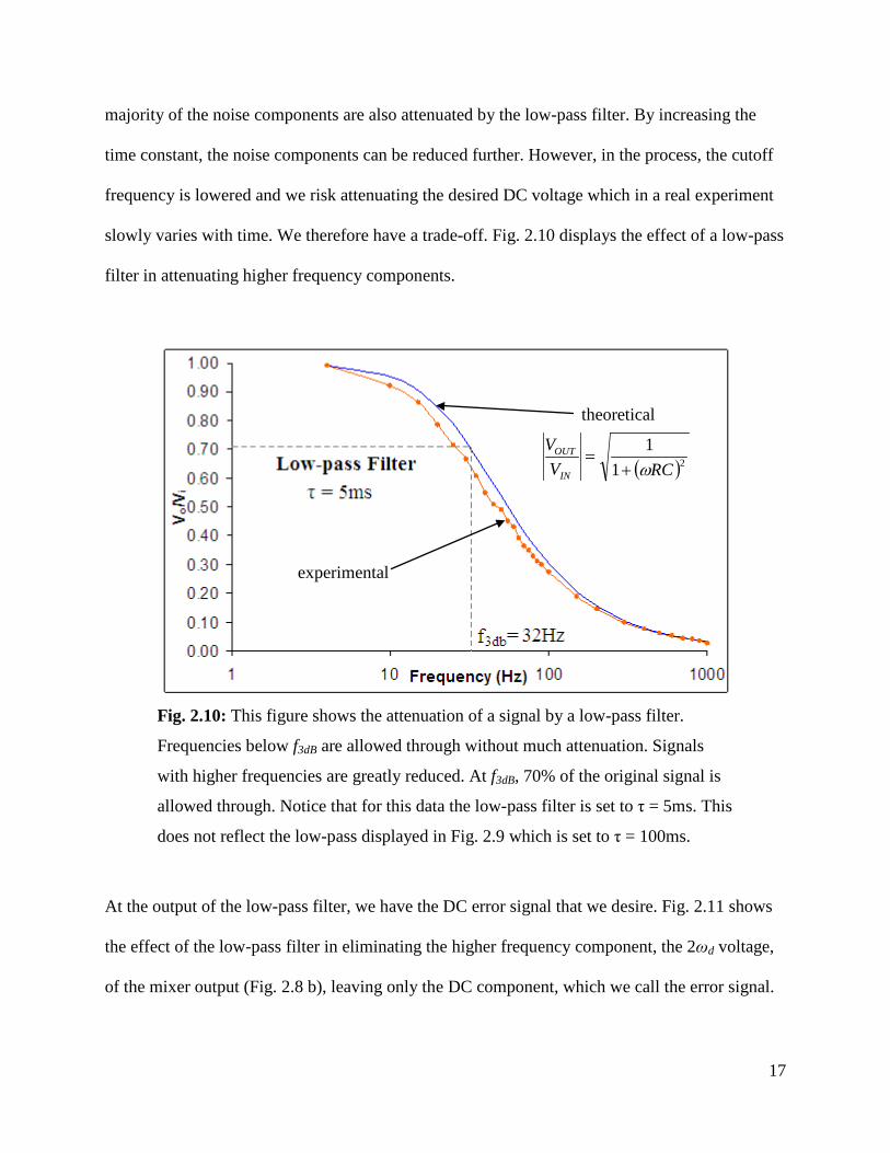
17

majority of the noise components are also attenuated by the low-pass filter. By increasing the

time constant, the noise components can be reduced further. However, in the process, the cutoff

frequency is lowered and we risk attenuating the desired DC voltage which in a real experiment

slowly varies with time. We therefore have a trade-off. Fig. 2.10 displays the effect of a low-pass

filter in attenuating higher frequency components.

Fig. 2.10: This figure shows the attenuation of a signal by a low-pass filter.

Frequencies below f3dB are allowed through without much attenuation. Signals

with higher frequencies are greatly reduced. At f3dB, 70% of the original signal is

allowed through. Notice that for this data the low-pass filter is set to τ = 5ms. This

does not reflect the low-pass displayed in Fig. 2.9 which is set to τ = 100ms.

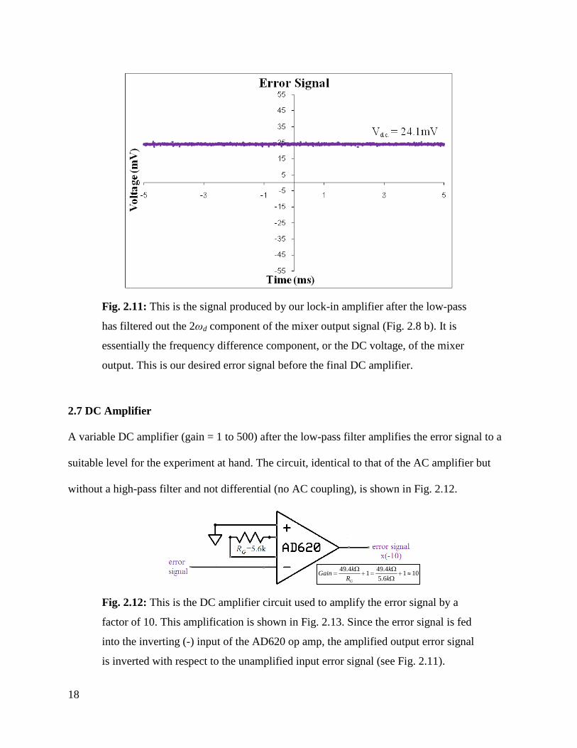
At the output of the low-pass filter, we have the DC error signal that we desire. Fig. 2.11 shows

the effect of the low-pass filter in eliminating the higher frequency component, the 2ωd voltage,

of the mixer output (Fig. 2.8 b), leaving only the DC component, which we call the error signal.

( )211RCV

VIN

OUT

ω+=

theoretical

experimental

18

Fig. 2.11: This is the signal produced by our lock-in amplifier after the low-pass

has filtered out the 2ωd component of the mixer output signal (Fig. 2.8 b). It is

essentially the frequency difference component, or the DC voltage, of the mixer

output. This is our desired error signal before the final DC amplifier.

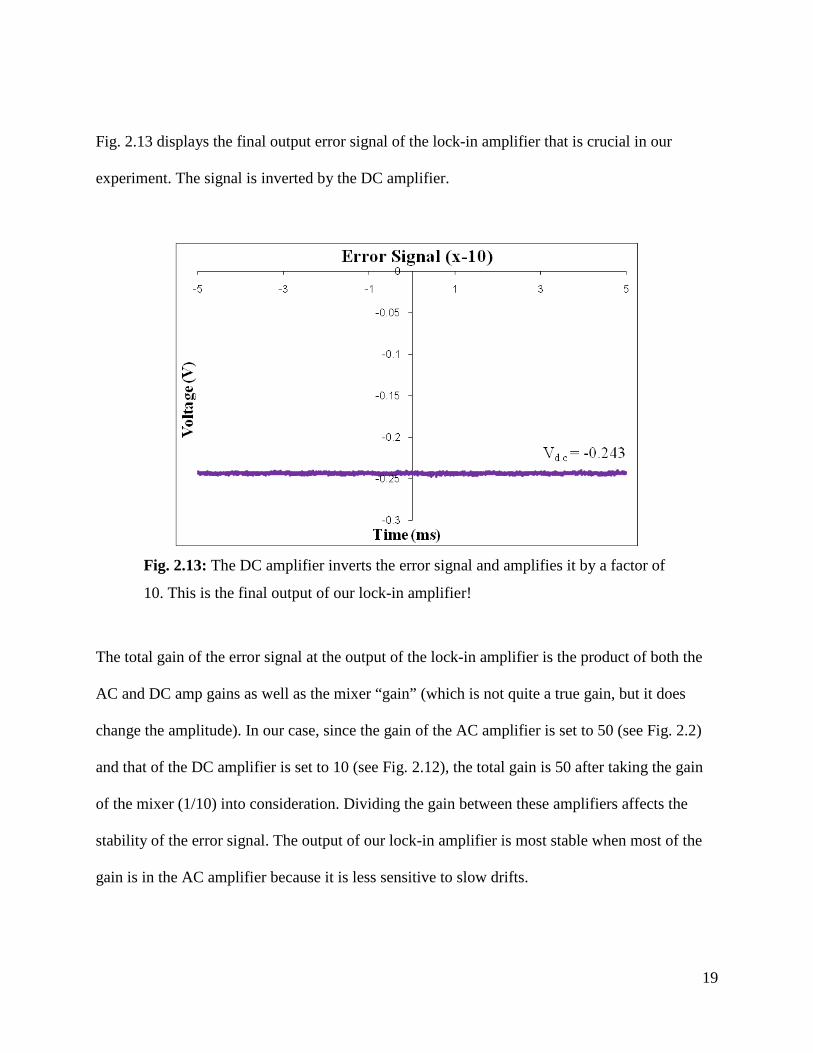
2.7 DC Amplifier

A variable DC amplifier (gain = 1 to 500) after the low-pass filter amplifies the error signal to a

suitable level for the experiment at hand. The circuit, identical to that of the AC amplifier but

without a high-pass filter and not differential (no AC coupling), is shown in Fig. 2.12.

Fig. 2.12: This is the DC amplifier circuit used to amplify the error signal by a

factor of 10. This amplification is shown in Fig. 2.13. Since the error signal is fed

into the inverting (-) input of the AD620 op amp, the amplified output error signal

is inverted with respect to the unamplified input error signal (see Fig. 2.11).

1016.54.4914.49

≈+ΩΩ

=+Ω

=kk

RkGain

G

19

Fig. 2.13 displays the final output error signal of the lock-in amplifier that is crucial in our

experiment. The signal is inverted by the DC amplifier.

Fig. 2.13: The DC amplifier inverts the error signal and amplifies it by a factor of

10. This is the final output of our lock-in amplifier!

The total gain of the error signal at the output of the lock-in amplifier is the product of both the

AC and DC amp gains as well as the mixer “gain” (which is not quite a true gain, but it does

change the amplitude). In our case, since the gain of the AC amplifier is set to 50 (see Fig. 2.2)

and that of the DC amplifier is set to 10 (see Fig. 2.12), the total gain is 50 after taking the gain

of the mixer (1/10) into consideration. Dividing the gain between these amplifiers affects the

stability of the error signal. The output of our lock-in amplifier is most stable when most of the

gain is in the AC amplifier because it is less sensitive to slow drifts.

20

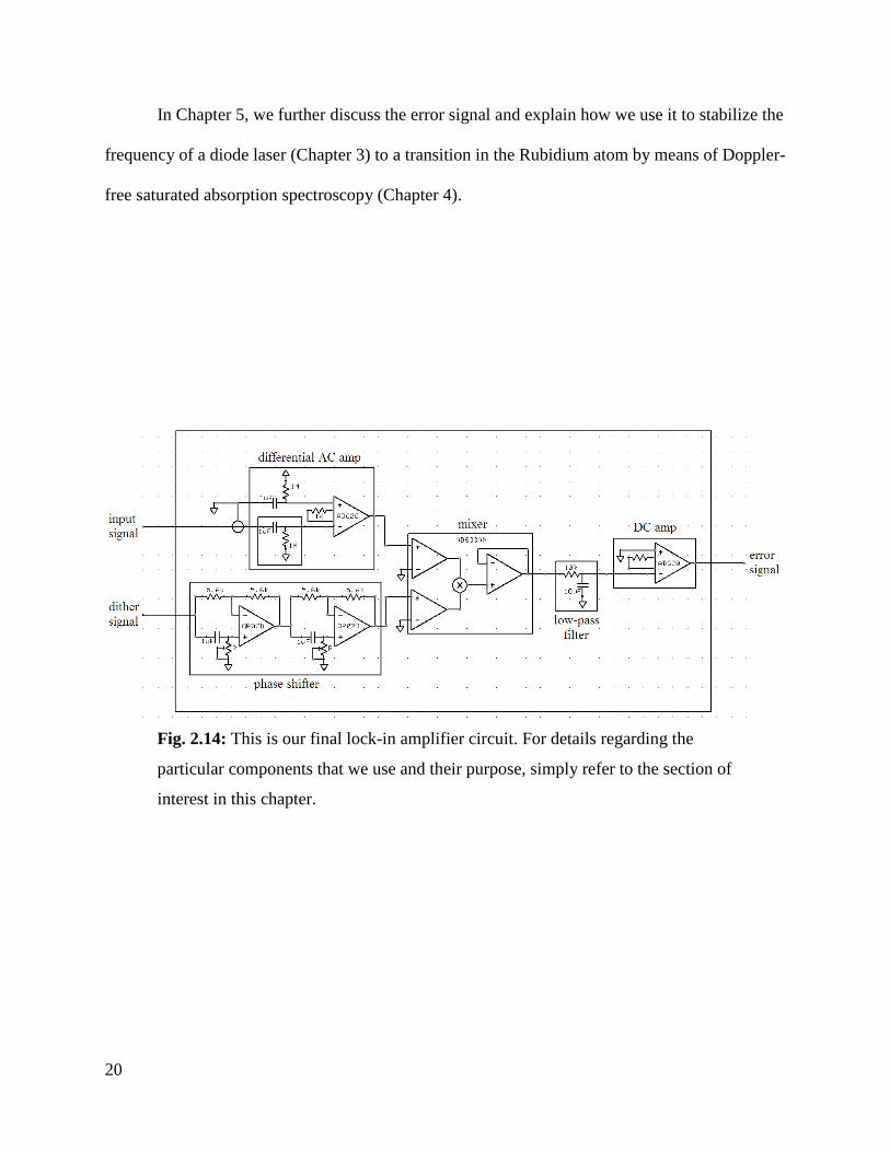
In Chapter 5, we further discuss the error signal and explain how we use it to stabilize the

frequency of a diode laser (Chapter 3) to a transition in the Rubidium atom by means of Doppler-

free saturated absorption spectroscopy (Chapter 4).

Fig. 2.14: This is our final lock-in amplifier circuit. For details regarding the

particular components that we use and their purpose, simply refer to the section of

interest in this chapter.

21

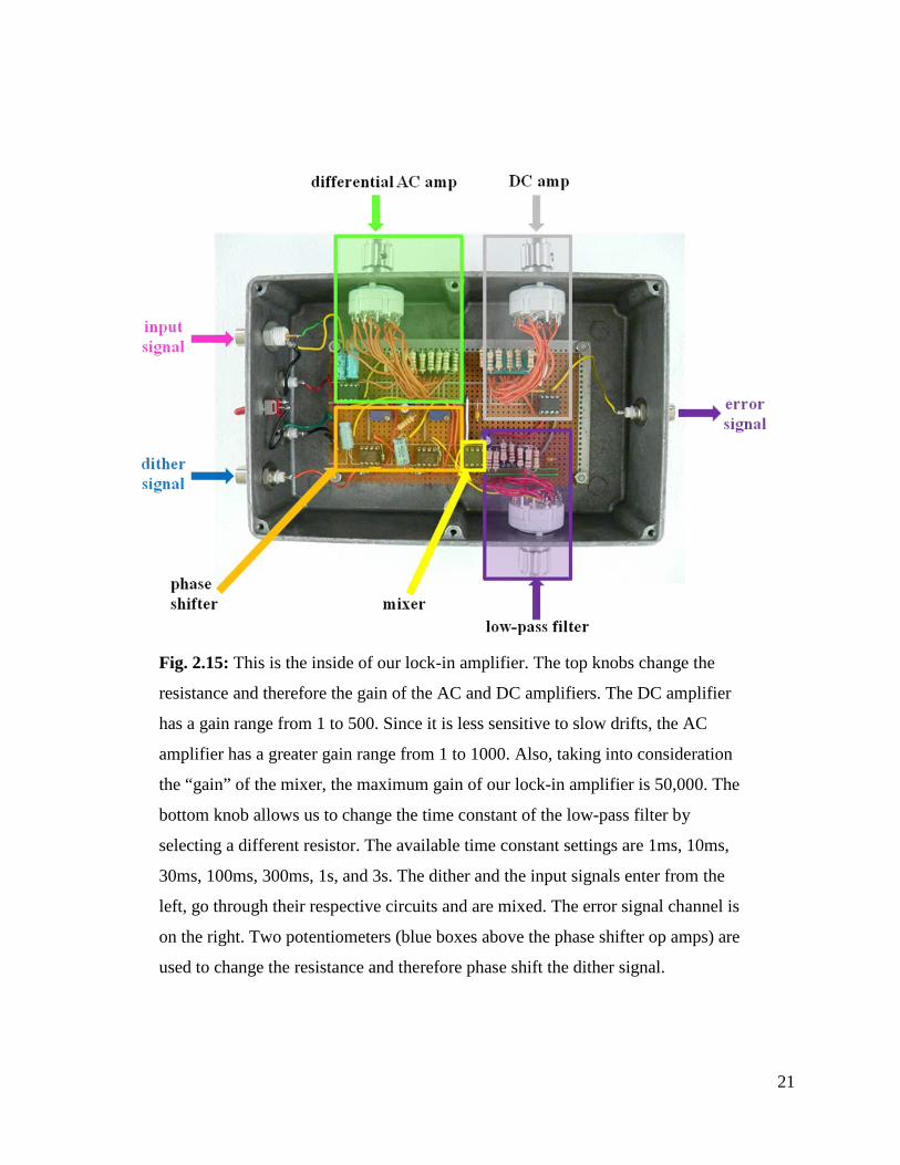
Fig. 2.15: This is the inside of our lock-in amplifier. The top knobs change the

resistance and therefore the gain of the AC and DC amplifiers. The DC amplifier

has a gain range from 1 to 500. Since it is less sensitive to slow drifts, the AC

amplifier has a greater gain range from 1 to 1000. Also, taking into consideration

the “gain” of the mixer, the maximum gain of our lock-in amplifier is 50,000. The

bottom knob allows us to change the time constant of the low-pass filter by

selecting a different resistor. The available time constant settings are 1ms, 10ms,

30ms, 100ms, 300ms, 1s, and 3s. The dither and the input signals enter from the

left, go through their respective circuits and are mixed. The error signal channel is

on the right. Two potentiometers (blue boxes above the phase shifter op amps) are

used to change the resistance and therefore phase shift the dither signal.

22

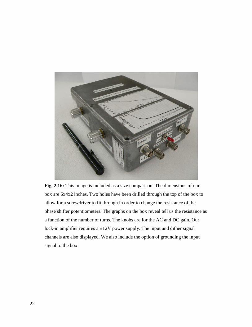
Fig. 2.16: This image is included as a size comparison. The dimensions of our

box are 6x4x2 inches. Two holes have been drilled through the top of the box to

allow for a screwdriver to fit through in order to change the resistance of the

phase shifter potentiometers. The graphs on the box reveal tell us the resistance as

a function of the number of turns. The knobs are for the AC and DC gain. Our

lock-in amplifier requires a ±12V power supply. The input and dither signal

channels are also displayed. We also include the option of grounding the input

signal to the box.

23

Chapter 3

Our Laser Setup and Frequency Tuning Parameters

3.1 Introduction

A laser diode emits a narrow range of frequencies. However, drifts in frequency occur over time

due, for example, to changes in laser temperature and current, as well as mechanical vibrations in

the apparatus. These frequency drifts make the laser unsuitable for experiments that require high

frequency stability. We want to make our laser operate at a specific frequency and keep it lasing

at that frequency for a long period of time (several hours) with very little or no drift.

There exist three important ways of adjusting the frequency of our laser. These are the

laser temperature, the electrical current (injection current) provided to the laser diode, and optical

feedback from a diffraction grating. By adjusting these parameters, the output frequency of our

laser diode can be tuned.

In this chapter, we describe the laser system that we assembled. Our laser setup consists

of five main parts: the laser diode, our mechanical setup, temperature control, injection current

control, and grating optical feedback control. The apparatus is shown in Fig. 3.1.

24

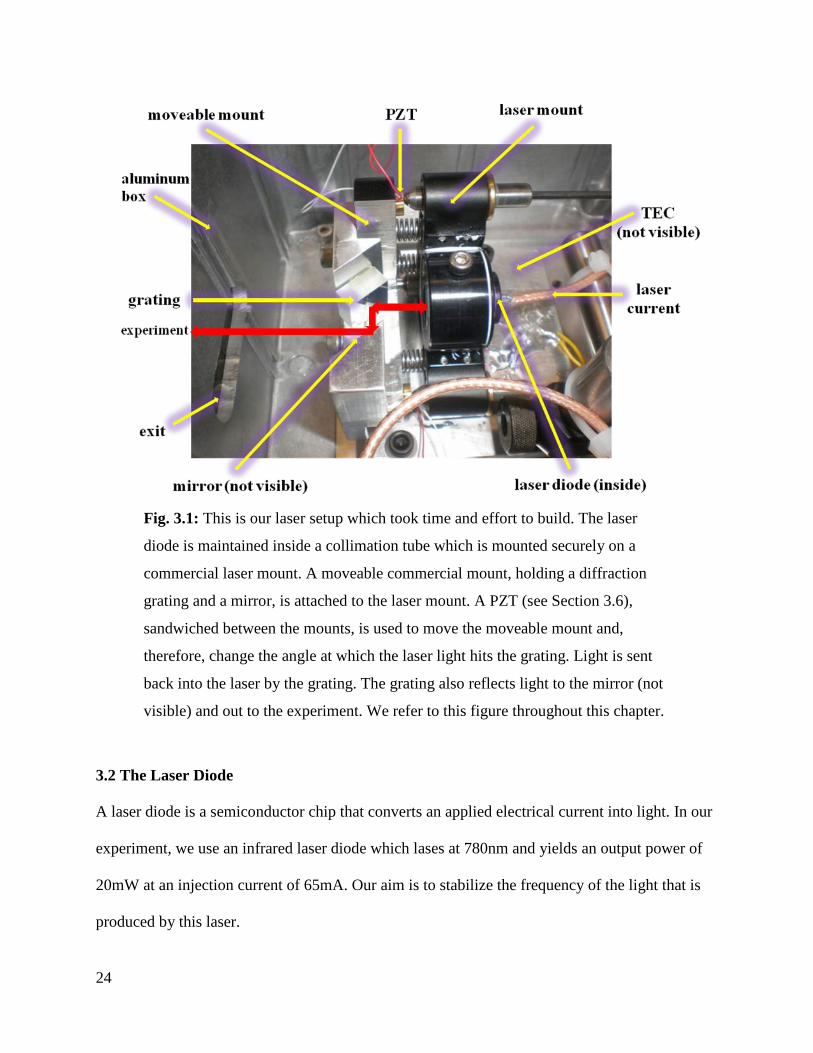
Fig. 3.1: This is our laser setup which took time and effort to build. The laser

diode is maintained inside a collimation tube which is mounted securely on a

commercial laser mount. A moveable commercial mount, holding a diffraction

grating and a mirror, is attached to the laser mount. A PZT (see Section 3.6),

sandwiched between the mounts, is used to move the moveable mount and,

therefore, change the angle at which the laser light hits the grating. Light is sent

back into the laser by the grating. The grating also reflects light to the mirror (not

visible) and out to the experiment. We refer to this figure throughout this chapter.

3.2 The Laser Diode

A laser diode is a semiconductor chip that converts an applied electrical current into light. In our

experiment, we use an infrared laser diode which lases at 780nm and yields an output power of

20mW at an injection current of 65mA. Our aim is to stabilize the frequency of the light that is

produced by this laser.

25

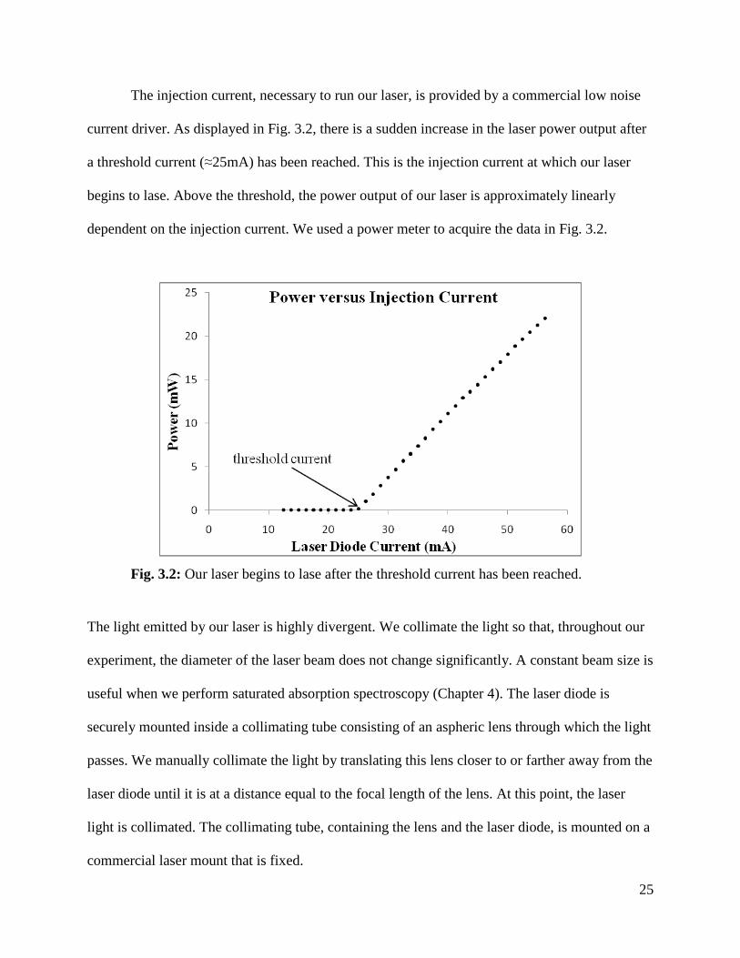
The injection current, necessary to run our laser, is provided by a commercial low noise

current driver. As displayed in Fig. 3.2, there is a sudden increase in the laser power output after

a threshold current (≈25mA) has been reached. This is the injection current at which our laser

begins to lase. Above the threshold, the power output of our laser is approximately linearly

dependent on the injection current. We used a power meter to acquire the data in Fig. 3.2.

Fig. 3.2: Our laser begins to lase after the threshold current has been reached.

The light emitted by our laser is highly divergent. We collimate the light so that, throughout our

experiment, the diameter of the laser beam does not change significantly. A constant beam size is

useful when we perform saturated absorption spectroscopy (Chapter 4). The laser diode is

securely mounted inside a collimating tube consisting of an aspheric lens through which the light

passes. We manually collimate the light by translating this lens closer to or farther away from the

laser diode until it is at a distance equal to the focal length of the lens. At this point, the laser

light is collimated. The collimating tube, containing the lens and the laser diode, is mounted on a

commercial laser mount that is fixed.

26

3.3 Our Mechanical Setup

A thermoelectric cooler (TEC) maintains the laser diode at a set temperature by actively cooling

or heating the entire mechanical setup. In order to ensure that the entire laser setup is at the same

temperature, all parts have been polished to ensure maximum surface contact between adjacent

surfaces. We also use heat-conducting thermal paste to optimize thermal conductivity.

The TEC is driven by a commercial temperature controller which stabilizes the

temperature of the laser to the set temperature within approximately 0.005°C. The TEC is

sandwiched between two conductive aluminum plates at the base of the laser mount and is

coupled to a thermistor: a resistor whose resistance varies with temperature. The thermistor,

buried inside the laser mount (not visible in Fig. 3.1), serves as a laser temperature sensor for the

controller.

The entire laser setup is mounted on an aluminum block which serves as a large heat

sink. The block is mounted stably on the optical table which provides vibrational and mechanical

stability and dampening. Our laser is covered with an aluminum box which blocks out any

unwanted light and air currents which interfere with the laser. The box has an opening just large

enough to allow the laser beam out. Lastly, to further block out any air currents and moisture, our

laser is also encased in a larger plexiglass box covered with material that absorbs sound waves

and keep out any light from the environment. The hole in this box is also just large enough to let

the laser light out.

27

3.4 First Tuning Parameter: Laser Temperature

Thermal expansion changes the cavity length of the semiconductor chip in the laser diode. An

increase in temperature increases the cavity length and increases the resonant wavelength. It also

shifts the semiconductor gain peak toward longer wavelengths (shorter frequencies). The laser

frequency can be changed by changing the temperature of the laser.

The temperature of the laser diode may be adjusted externally. We can vary the

temperature from 15 to 40°C, and a typical temperature tuning is 0.03 nm/°C, or 15GHz/°C. The

advantage of using this tuning parameter is that large changes in frequency are possible.

However, there are disadvantages. First of all, it can take up to half an hour for the temperature

of the laser to stabilize completely. Also, with this tuning parameter it is very difficult to make

small changes in laser frequency, and so the tuning that can be achieved is very coarse.

3.5 Second Tuning Parameter: Injection Current

Unlike direct temperature control, the injection current raises the laser temperature internally by

means of joule heating. Increased electron density also changes the refractive index. As a result,

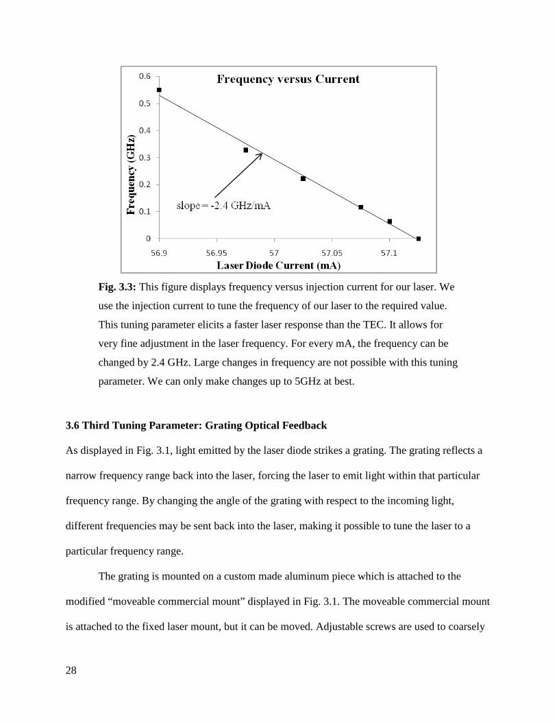
the response from laser current tuning is faster than from external heating. We measured the

variation of laser frequency with injection current as shown in Fig. 3.3. There is a linear

dependence of laser frequency on current. For every mA change in the injection current, the laser

frequency changes by 2.4GHz. We use this tuning parameter extensively to tune the frequency of

our laser.

28

Fig. 3.3: This figure displays frequency versus injection current for our laser. We

use the injection current to tune the frequency of our laser to the required value.

This tuning parameter elicits a faster laser response than the TEC. It allows for

very fine adjustment in the laser frequency. For every mA, the frequency can be

changed by 2.4 GHz. Large changes in frequency are not possible with this tuning

parameter. We can only make changes up to 5GHz at best.

3.6 Third Tuning Parameter: Grating Optical Feedback

As displayed in Fig. 3.1, light emitted by the laser diode strikes a grating. The grating reflects a

narrow frequency range back into the laser, forcing the laser to emit light within that particular

frequency range. By changing the angle of the grating with respect to the incoming light,

different frequencies may be sent back into the laser, making it possible to tune the laser to a

particular frequency range.

The grating is mounted on a custom made aluminum piece which is attached to the

modified “moveable commercial mount” displayed in Fig. 3.1. The moveable commercial mount

is attached to the fixed laser mount, but it can be moved. Adjustable screws are used to coarsely

29

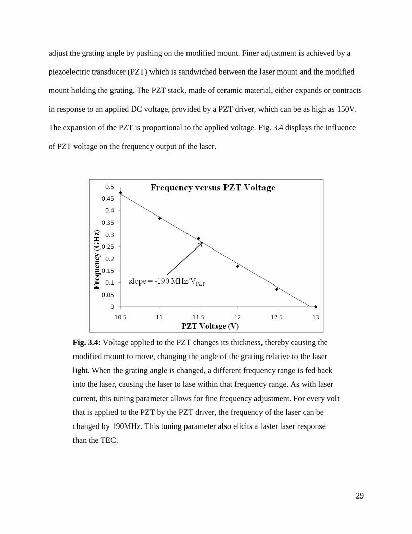
adjust the grating angle by pushing on the modified mount. Finer adjustment is achieved by a

piezoelectric transducer (PZT) which is sandwiched between the laser mount and the modified

mount holding the grating. The PZT stack, made of ceramic material, either expands or contracts

in response to an applied DC voltage, provided by a PZT driver, which can be as high as 150V.

The expansion of the PZT is proportional to the applied voltage. Fig. 3.4 displays the influence

of PZT voltage on the frequency output of the laser.

Fig. 3.4: Voltage applied to the PZT changes its thickness, thereby causing the

modified mount to move, changing the angle of the grating relative to the laser

light. When the grating angle is changed, a different frequency range is fed back

into the laser, causing the laser to lase within that frequency range. As with laser

current, this tuning parameter allows for fine frequency adjustment. For every volt

that is applied to the PZT by the PZT driver, the frequency of the laser can be

changed by 190MHz. This tuning parameter also elicits a faster laser response

than the TEC.

30

3.7 Closing Remarks

The tuning parameters presented in this chapter make it possible to control the frequency output

of our laser. At the level of precision that we need for our experiment, however, the laser is not

adequately stabilized by simply adjusting these parameters and holding them constant.

Therefore, we need a way of continuously adjusting these parameters so that the laser frequency

does not deviate from a stable reference frequency. We discuss in Chapter 5 how the signal from

our lock-in amplifier can be used in a negative feedback loop to stabilize the frequency of our

laser. However, we must first establish a reference frequency. This is covered in Chapter 4.

31

Chapter 4

Our Optical Setup and Saturated Absorption Spectroscopy 4.1 Introduction

In order to stabilize the frequency of our laser, we need a highly stable optical reference

frequency. The hyperfine atomic transitions of the Rubidium-85 isotope provide the level of

stability that we need. We use a technique known as Doppler-free saturated absorption

spectroscopy to produce a spectrum of narrow peaks to which we can lock the frequency of our

laser by means of feedback from our lock-in amplifier. These peaks correspond to different

hyperfine transitions of 85Rb. By carefully adjusting the laser temperature, injection current, and

grating angle, as described in Chapter 3, our laser can be tuned to one of these hyperfine atomic

transitions.

Our optical setup is divided into two main parts: a laser frequency monitoring section and

the Doppler-free saturated absorption apparatus. Fig. 4.1 displays our overall setup.

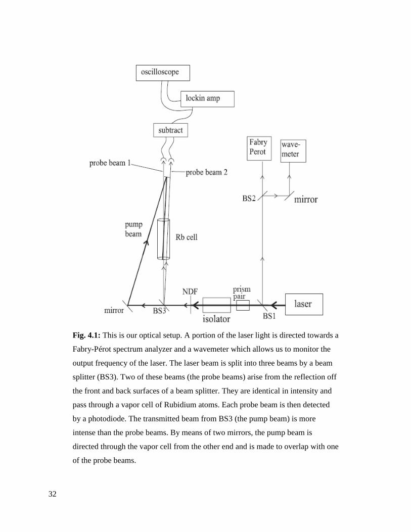
32

Fig. 4.1: This is our optical setup. A portion of the laser light is directed towards a

Fabry-Pérot spectrum analyzer and a wavemeter which allows us to monitor the

output frequency of the laser. The laser beam is split into three beams by a beam

splitter (BS3). Two of these beams (the probe beams) arise from the reflection off

the front and back surfaces of a beam splitter. They are identical in intensity and

pass through a vapor cell of Rubidium atoms. Each probe beam is then detected

by a photodiode. The transmitted beam from BS3 (the pump beam) is more

intense than the probe beams. By means of two mirrors, the pump beam is

directed through the vapor cell from the other end and is made to overlap with one

of the probe beams.

33

4.2 Monitoring the Laser Frequency

Before entering the setup for saturation absorption spectroscopy, a small portion of the laser light

is immediately deflected aside by BS1 for monitoring purposes. In order to tune the laser

frequency to the precise level of an atomic reference frequency, it is important to constantly

know the characteristics of the laser light.

A Fabry-Pérot spectrum analyzer makes it possible to determine if the laser is emitting a

single or multiple wavelengths of light. This device is made up of two mirrors facing one another

that are spaced in such a way that only light with a certain wavelength resonates in the space (the

cavity) between the mirrors. One of these mirrors is fixed, while the other is moved (or scanned)

back and forth, changing the cavity length. Typically, at two points in the scan, resonance is

achieved. A photodiode behind the mirror cavity monitors the resonant transmission and displays

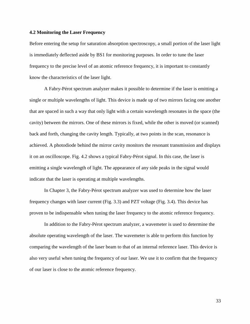
it on an oscilloscope. Fig. 4.2 shows a typical Fabry-Pérot signal. In this case, the laser is

emitting a single wavelength of light. The appearance of any side peaks in the signal would

indicate that the laser is operating at multiple wavelengths.

In Chapter 3, the Fabry-Pérot spectrum analyzer was used to determine how the laser

frequency changes with laser current (Fig. 3.3) and PZT voltage (Fig. 3.4). This device has

proven to be indispensable when tuning the laser frequency to the atomic reference frequency.

In addition to the Fabry-Pérot spectrum analyzer, a wavemeter is used to determine the

absolute operating wavelength of the laser. The wavemeter is able to perform this function by

comparing the wavelength of the laser beam to that of an internal reference laser. This device is

also very useful when tuning the frequency of our laser. We use it to confirm that the frequency

of our laser is close to the atomic reference frequency.

34

Fig. 4.2: The Fabry-Pérot spectrum analyzer, composed of two mirrors and a

photodiode, allows us to ensure that the laser is operating at a single wavelength

of light. One mirror is fixed and the other one is moved back and forth. As

described in the text, two signals are detected, and for our particular Fabry-Pérot

cavity these two peaks are 1500MHz apart.

Backscattered light from any of the components in our optical setup could very easily destabilize

the frequency of our laser. Unwanted optical feedback adds frequencies that would compete with

the frequency being fed back to the laser by the grating. In order to deal with this problem, an

isolator is included in our setup. This optical element helps to prevent unwanted optical feedback

by allowing the transmission of the laser light in only one direction. We also keep track of

harmful reflections and slightly misalign, on purpose, some of our optical elements, such as the

Fabry-Pérot spectrum analyzer, so that the light it reflects is directed to a point where it cannot

get into our laser. Apertures are also used, where necessary and where they do not cause

backscattering, to block unwanted beams.

35

4.3 Rubidium Vapor Cell

Our saturation absorption spectroscopy setup includes a vapor cell of Rubidium atoms

maintained at room temperature. The atomic transition of 85Rb, occurring at a very specific

wavelength of 780.245nm, provides a highly stable reference frequency for locking our laser.

When the laser is tuned precisely to the atomic transition frequency, absorption of the laser light

by atoms in the 5s ground state takes place (see Fig. 4.3). These atoms become excited as their

electrons are promoted to the 5p excited state. When these excited atoms eventually decay back

into the ground state, fluorescence occurs as the absorbed light is re-emitted in all directions.

Along with the wavemeter, we can use an observation of fluorescence to confirm that the laser is

at the correct frequency to excite 85Rb. The atomic transition of 85Rb, in fact, branches off into

three hyperfine atomic transitions each of which occurs at a unique frequency. These transitions

are the F=3 to F’=2, 3, or 4 transitions displayed in Fig. 4.3.

Since the Rubidium atoms in the cell are in a gaseous phase, they are in constant motion

because of their thermal energy. These atoms are characterized by different velocity classes

according to the magnitude of their speed and direction of motion. The zero velocity class, in

particular, refers to those atoms that are not moving.

36

Fig. 4.3: This is the 85Rb level diagram. Transitions from a ground state to an

excited state must follow quantum mechanical selection rules. In the case of the

transitions from the F=3 ground state energy level for 85Rb to the four F’ excited

state energy levels, there can only be three possible transitions, as illustrated.

4.4 Doppler-Broadened Absorption Spectrum

When the laser frequency is on resonance with the atomic transition frequency of 85Rb, some of

the laser light is absorbed by the atoms. As a result, the photodiodes detect less light from the

probe beams. By scanning the frequency of our laser back and forth across the atomic transition

frequency of 85Rb, we produce an absorption spectrum (see Fig. 1.1). Intuitively, this spectrum

should consist of narrow dips which correspond to the hyperfine transition frequencies of 85Rb.

However, these dips are broadened due to a phenomenon called Doppler-broadening.

37

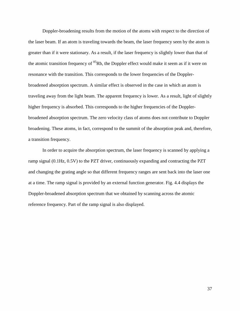
Doppler-broadening results from the motion of the atoms with respect to the direction of

the laser beam. If an atom is traveling towards the beam, the laser frequency seen by the atom is

greater than if it were stationary. As a result, if the laser frequency is slightly lower than that of

the atomic transition frequency of 85Rb, the Doppler effect would make it seem as if it were on

resonance with the transition. This corresponds to the lower frequencies of the Doppler-

broadened absorption spectrum. A similar effect is observed in the case in which an atom is

traveling away from the light beam. The apparent frequency is lower. As a result, light of slightly

higher frequency is absorbed. This corresponds to the higher frequencies of the Doppler-

broadened absorption spectrum. The zero velocity class of atoms does not contribute to Doppler

broadening. These atoms, in fact, correspond to the summit of the absorption peak and, therefore,

a transition frequency.

In order to acquire the absorption spectrum, the laser frequency is scanned by applying a

ramp signal (0.1Hz, 0.5V) to the PZT driver, continuously expanding and contracting the PZT

and changing the grating angle so that different frequency ranges are sent back into the laser one

at a time. The ramp signal is provided by an external function generator. Fig. 4.4 displays the

Doppler-broadened absorption spectrum that we obtained by scanning across the atomic

reference frequency. Part of the ramp signal is also displayed.

38

Fig. 4.4: This is a portion of the Doppler-broadened saturated absorption

spectrum obtained by scanning the laser frequency across the atomic transition of 85Rb. We observe a dip instead of a peak (as in Fig 1.1) because absorption of

light results in a decrease in light to the photodiodes. The theoretical Doppler-

broadened absorption spectrum has a full width half maximum of about 500MHz.

Limited by our scanning range, we were only able to observe a portion of the dip.

4.5 Probe and Pump Beams

As displayed in Fig. 4.1, The main laser beam is split into three less intense beams: two probe

beams and a pump beam. All three beams go through the Rubidium cell and are at the same

frequency, but differ in intensity and direction of travel.

Two weak probe beams of approximately equal intensity (7% of the main beam intensity)

are formed by the reflection of the laser beam off the front and back surfaces of BS3. As these

identical beams pass through the 85Rb vapor cell, they interact with the same velocity class of

atoms. After the cell, each is detected by a photodiode which is sensitive to the infrared light.

39

Since it is transmitted through BS-3, the pump beam is much more intense (93% of the

main beam intensity) than the probe beams. By means of two carefully-placed adjustable

mirrors, the pump beam enters the Rubidium cell from the opposite end and is overlapped with

one of the probe beams. Since the pump beam is at the same frequency as the probe beams, it

interacts with a similar velocity class of atoms, but which travel in the opposite direction.

When the laser frequency is not on resonance with the atomic transition frequency of

85Rb, the pump and the probe beams interact with different atoms traveling at the same speed,

but in opposite directions. On the other hand, when the pump and the probe beams are on

resonance with the atomic transition, they excite the same zero velocity class of atoms, which

correspond to the transitions. When this happens, the pump and the probe beams compete for

atoms to excite. Since the pump beam is much more intense than the probe beams, it has a

greater probability of exciting these atoms. The pump beam significantly “saturates” the

transition, reducing (by up to 50%) the number of atoms in the ground state available to the

probe beam to excite. This phenomenon between the pump and the probe beams forms the basis

of a technique for determining the hyperfine atomic transition frequencies of an atom. This

technique is called saturated absorption spectroscopy.

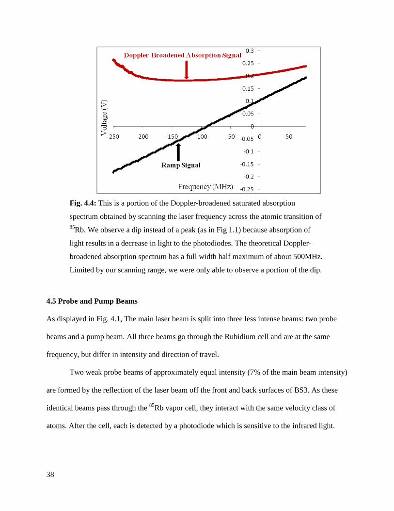
4.6 Saturated Absorption Spectroscopy

The reduction by the pump beam of the number of atoms in the ground state when the laser is on

resonance results in a reduction of the absorption of probe beam 1. More light is therefore

detected by the photodiode and peaks form in the Doppler-broadened absorption spectrum (see

Fig. 4.5). These narrow features correspond to each of the hyperfine atomic transitions of 85Rb,

as indicated in the figure.

40

Additional peaks (labeled “X” in Fig. 2.5), called “crossovers,” occur when the frequency

of our laser falls exactly halfway between a pair of atomic transition frequencies. Both the pump

and the probe beams excite atoms from the ground state, but to different excited states at the

same time. In this case, the pump and the probe beams interact with the same nonzero velocity

class of atoms. As a result, as in the case of the zero velocity class of atoms, there is a reduction

in the absorption of the probe beam and consequently a detected absorption peak.

Fig. 4.5: This is the saturated absorption spectrum formed when the frequency of

our laser is scanned across the atomic transitions. The saturated absorption

spectrum consists of a sequence of peaks superimposed on the Doppler-broadened

spectrum. These peaks occur when the pump and probe beam 1 are resonant with

each of the three hyperfine atomic transitions of 85Rb. Crossovers occurs when the

laser frequency is halfway between two transitions. Since three hyperfine atomic

transitions are possible, there exist three crossovers between: F’= 23, 34, and

24. We maximize the amplitude of all of these peaks by having the pump beam

and probe beam 1 overlap as much as possible (forming an angle of about 1°).

41

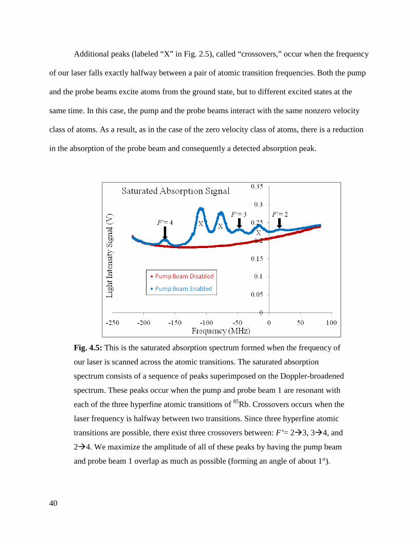
Probe beam 2, unaffected by the pump beam, reports the Doppler-broadened absorption

spectrum (Fig. 4.4). The Doppler background is eliminated by subtracting the signals from probe

beams 1 and 2 (see Fig. 4.6). The resulting Doppler-free saturated absorption signal consists of

spectral peaks that correspond to regions of decreased absorption, or increased light to PD1.

Fig. 4.6: This is the Doppler-free saturated absorption spectrum obtained by

taking the difference between the signals (Fig. 4.5) from probe beams 1 and 2.

4.7 Improving the Saturated Absorption Signal

For the hyperfine atomic transitions of 85Rb, the intensity required for saturation, Is, is

1.6mW/cm2. After the optical isolator, we include a 20dB neutral density filter (NDF) which

transmits 1% of the laser light. Without affecting the laser frequency, the NDF attenuates the

light, providing a suitable pump beam intensity (2.7mW/cm2 ≈ Is) and probe beam intensity

(0.6mW/cm2 < Is) for observing the saturated absorption spectrum with well-defined peaks. Fig.

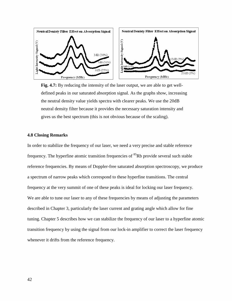
4.7 shows the effects of varying the pump and probe beam intensities by using different NDFs.

42

Fig. 4.7: By reducing the intensity of the laser output, we are able to get well-

defined peaks in our saturated absorption signal. As the graphs show, increasing

the neutral density value yields spectra with clearer peaks. We use the 20dB

neutral density filter because it provides the necessary saturation intensity and

gives us the best spectrum (this is not obvious because of the scaling).

4.8 Closing Remarks

In order to stabilize the frequency of our laser, we need a very precise and stable reference

frequency. The hyperfine atomic transition frequencies of 85Rb provide several such stable

reference frequencies. By means of Doppler-free saturated absorption spectroscopy, we produce

a spectrum of narrow peaks which correspond to these hyperfine transitions. The central

frequency at the very summit of one of these peaks is ideal for locking our laser frequency.

We are able to tune our laser to any of these frequencies by means of adjusting the parameters

described in Chapter 3, particularly the laser current and grating angle which allow for fine

tuning. Chapter 5 describes how we can stabilize the frequency of our laser to a hyperfine atomic

transition frequency by using the signal from our lock-in amplifier to correct the laser frequency

whenever it drifts from the reference frequency.

43

Chapter 5

Stabilizing the Frequency of Our Laser

5.1 Introduction

The key to stabilizing the frequency of our laser is using a negative feedback signal, produced by

our lock-in amplifier, that continuously forces the laser back onto the peak of a hyperfine atomic

transition as the laser frequency naturally drifts in one direction or the other, away from the peak.

In locking the frequency of our laser to a hyperfine atomic transition frequency in 85Rb,

the only tuning parameter that we manipulate is the grating angle. The error signal, fed to the

PZT, continuously changes the grating angle so the laser frequency stays locked onto the point

where there is no 1ωd signal as measured by the lock-in amplifier. This will keep our laser stable

at a hyperfine atomic transition of 85Rb.

5.2 Dither and Input Signals

A dither signal (2V, ωd = 512Hz) is provided to our lock-in amplifier by an external sine wave

generator. After being attenuated by -40dB, this dither signal (now 0.2mV) also goes to the PZT

driver. The dither signal causes the PZT to expand and contract, dithering the grating angle and

therefore the laser frequency. The dithered laser light is sent through the cell. Our experiment

responds at the same frequency ωd, providing the input signal for our lock-in amplifier. The

input signal is the Doppler-free saturated absorption signal as described in Chapter 4.

44

5.3 The Error Signal

When our lock-in amplifier is provided with both the input signal (Eq. 5.1) and the dither signal

(Eq. 5.2), it generates a DC error signal that is proportional to the amplitude of 1ωd signal

present in the input signal, A. The mixer in our lock-in amplifier multiplies the dither and input

signals together to produce a mixed signal (Eq. 5.3) with the sum and difference frequency

components. Assuming that these signals have been made in phase by the phase shifters of our

lock-in amplifier, the output of the mixer is given by Eq. 5.3.

( )tAVin ωsin= [Eq. 5.1]

( )tBV dd ωsin= [Eq. 5.2]

( ) ( )[ ]ttttABV ddmixed ωωωω +−−= coscos

2 [Eq. 5.3]

As displayed in Fig. 5.1, when the laser frequency is on resonance with the atomic

transition frequency, one dither cycle passes twice over the absorption peak, producing a 2ωd

absorption signal. This signal is detected by the photodiodes and is fed into the input channel of

our lock-in amplifier. In this case ω = 2ωd. So, Eq. 5.1 becomes

( )tAV din ω2sin= [Eq. 5.4]

This input signal is multiplied with the dither signal (Eq. 5.2). The resulting mixed signal

contains a 1ωd difference frequency component and a 3ωd sum frequency component,

( ) ( )[ ]ttABV ddmixed ωω 3cos1cos

2−=

[Eq. 5.5]

The amplitudes of both of these frequency components are reduced by the low-pass filter in our

lock-in amplifier. Hence, no DC error signal is produced when the laser frequency is on

resonance with the atomic transition frequency, as desired.

45

On the other hand, when the laser frequency is not on resonance with the atomic

transition frequency, one dither cycle produces a 1ωd absorption signal. In this case, the input

becomes a 1ωd signal (i.e. ω = ωd) as displayed in Fig. 5.1, and so,

( )tAV din ωsin= [Eq. 5.6]

This input signal is multiplied with the dither signal (Eq. 5.2). The resulting mixed signal

contains a 0ωd (i.e. DC) difference frequency component and a 2ωd sum frequency component,

( ) ( )[ ] ( )[ ]tABttABV dddmixed ωωω 2cos1

22cos0cos

2−=−=

[Eq. 5.7]

The 2ωd sum component is eliminated by means of the low-pass filter, leaving only the DC

voltage, which is the error signal. Hence, an error signal is produced whenever the laser

frequency is not on resonance with the atomic transition frequency. As displayed in Fig. 5.2, the

magnitude and sign of this error signal depend on how far off and in what direction the laser

frequency is with respect to the atomic reference frequency.

46

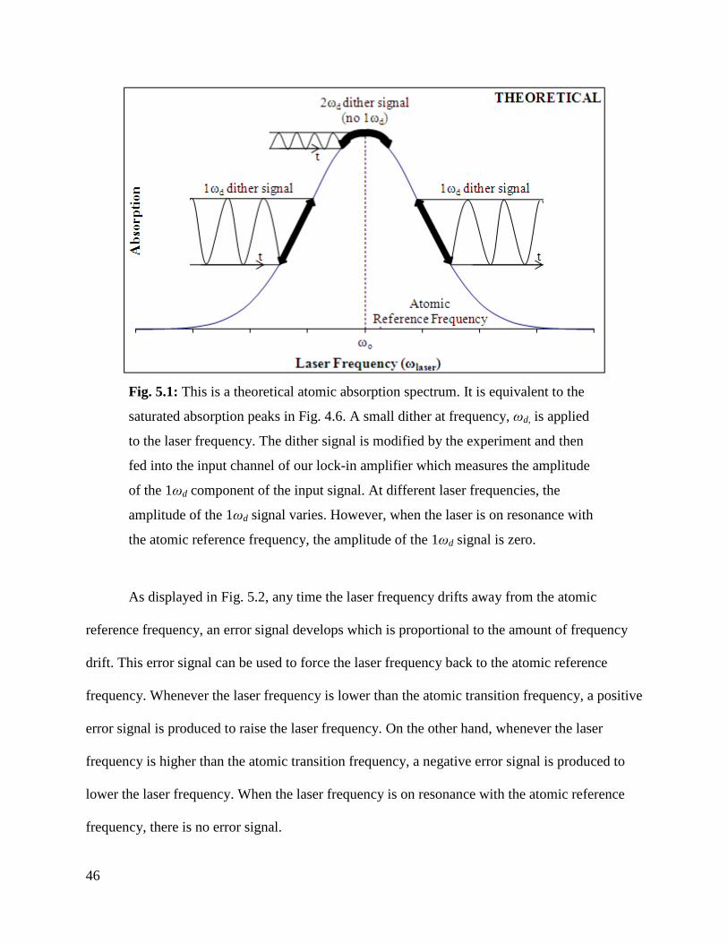
Fig. 5.1: This is a theoretical atomic absorption spectrum. It is equivalent to the

saturated absorption peaks in Fig. 4.6. A small dither at frequency, ωd, is applied

to the laser frequency. The dither signal is modified by the experiment and then

fed into the input channel of our lock-in amplifier which measures the amplitude

of the 1ωd component of the input signal. At different laser frequencies, the

amplitude of the 1ωd signal varies. However, when the laser is on resonance with

the atomic reference frequency, the amplitude of the 1ωd signal is zero.

As displayed in Fig. 5.2, any time the laser frequency drifts away from the atomic

reference frequency, an error signal develops which is proportional to the amount of frequency

drift. This error signal can be used to force the laser frequency back to the atomic reference

frequency. Whenever the laser frequency is lower than the atomic transition frequency, a positive

error signal is produced to raise the laser frequency. On the other hand, whenever the laser

frequency is higher than the atomic transition frequency, a negative error signal is produced to

lower the laser frequency. When the laser frequency is on resonance with the atomic reference

frequency, there is no error signal.

47

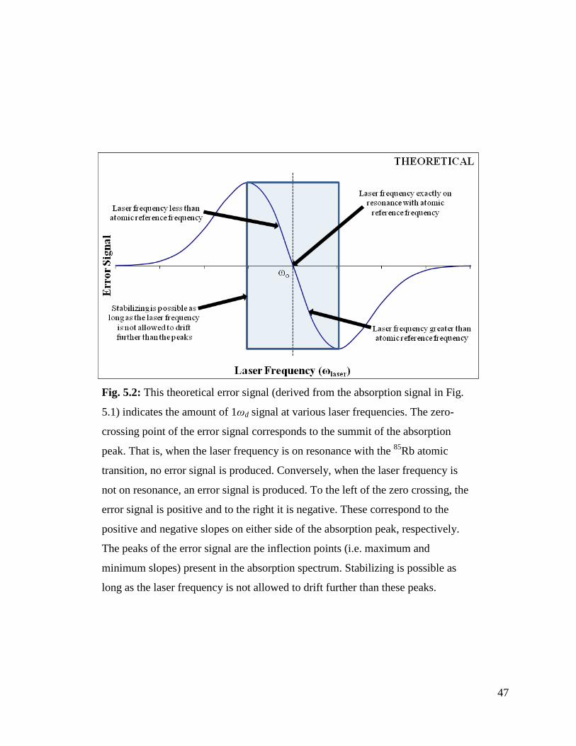
Fig. 5.2: This theoretical error signal (derived from the absorption signal in Fig.

5.1) indicates the amount of 1ωd signal at various laser frequencies. The zero-

crossing point of the error signal corresponds to the summit of the absorption

peak. That is, when the laser frequency is on resonance with the 85Rb atomic

transition, no error signal is produced. Conversely, when the laser frequency is

not on resonance, an error signal is produced. To the left of the zero crossing, the

error signal is positive and to the right it is negative. These correspond to the

positive and negative slopes on either side of the absorption peak, respectively.

The peaks of the error signal are the inflection points (i.e. maximum and

minimum slopes) present in the absorption spectrum. Stabilizing is possible as

long as the laser frequency is not allowed to drift further than these peaks.

48

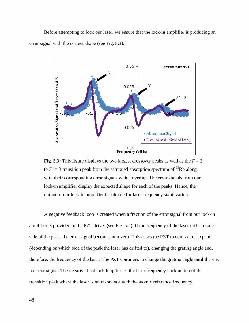
Before attempting to lock our laser, we ensure that the lock-in amplifier is producing an

error signal with the correct shape (see Fig. 5.3).

Fig. 5.3: This figure displays the two largest crossover peaks as well as the F = 3

to F’ = 3 transition peak from the saturated absorption spectrum of 85Rb along

with their corresponding error signals which overlap. The error signals from our

lock-in amplifier display the expected shape for each of the peaks. Hence, the

output of our lock-in amplifier is suitable for laser frequency stabilization.

A negative feedback loop is created when a fraction of the error signal from our lock-in

amplifier is provided to the PZT driver (see Fig. 5.4). If the frequency of the laser drifts to one

side of the peak, the error signal becomes non-zero. This cases the PZT to contract or expand

(depending on which side of the peak the laser has drifted to), changing the grating angle and,

therefore, the frequency of the laser. The PZT continues to change the grating angle until there is

no error signal. The negative feedback loop forces the laser frequency back on top of the

transition peak where the laser is on resonance with the atomic reference frequency.

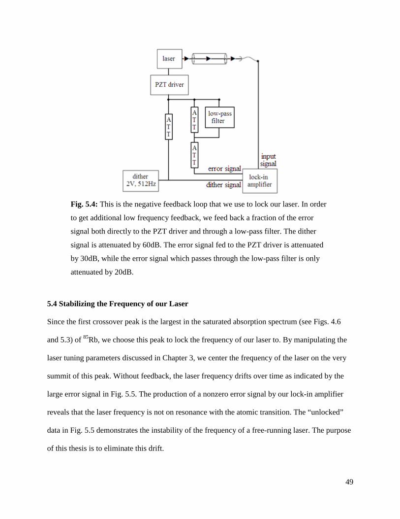
49

Fig. 5.4: This is the negative feedback loop that we use to lock our laser. In order

to get additional low frequency feedback, we feed back a fraction of the error

signal both directly to the PZT driver and through a low-pass filter. The dither

signal is attenuated by 60dB. The error signal fed to the PZT driver is attenuated

by 30dB, while the error signal which passes through the low-pass filter is only

attenuated by 20dB.

5.4 Stabilizing the Frequency of our Laser

Since the first crossover peak is the largest in the saturated absorption spectrum (see Figs. 4.6

and 5.3) of 85Rb, we choose this peak to lock the frequency of our laser to. By manipulating the

laser tuning parameters discussed in Chapter 3, we center the frequency of the laser on the very

summit of this peak. Without feedback, the laser frequency drifts over time as indicated by the

large error signal in Fig. 5.5. The production of a nonzero error signal by our lock-in amplifier

reveals that the laser frequency is not on resonance with the atomic transition. The “unlocked”

data in Fig. 5.5 demonstrates the instability of the frequency of a free-running laser. The purpose

of this thesis is to eliminate this drift.

50

When the feedback loop is enabled, however, we see that the error signal is nearly zero,

meaning that the laser frequency is locked on the atomic transition. Without feedback, the laser

frequency drifts away from the transition peak in less than 1 minute, producing a large error

signal. On the other hand, with feedback, the laser frequency stays locked on the atomic

transition for 40 minutes, producing a very small error signal. The data shows that the error

signal from our lock-in amplifier was able to maintain our laser stable at a specific frequency for

a very reasonable amount of time.

Fig. 5.5: Without feedback from our lock-in amplifier, the frequency of our laser

drifts away from the transition peak in less than 1 minute, producing a large error

signal. However, when the feedback is enabled, our lock-in amplifier is able to

lock the laser to the atomic transition of 85Rb as displayed by the nearly zero error

signal. A jump in the laser frequency occurred around t = 18min, but the lock-in

amplifier was able to regain the lock. The frequency of our laser became unstable

shortly after the 40 minutes that it took to record this data.

Since the largest crossover peak that we locked to is 5MHz wide at half maximum (see Fig. 5.3)

and we stay locked on top, our laser frequency is certainly stabilized to less than 5MHz. This

represents a fractional frequency stability of better than 10-8 over the 40 minute period.

51

Conclusion

The locked data in Fig. 5.5 represents the achievement of our goal of stabilizing the frequency of

our laser. We have reached this goal by building and assembling every part of the system

ourselves, from the lock-in amplifier to the laser system, and saturated absorption spectroscopy

setup. After a lot of time and effort, we have also gained a valuable understanding about the

operation and function of every component in our experiment.

The stability of the lock in Fig. 5.5 is affected by the total gain (product of AC and DC

amplifier gains) of the error signal from our lock-in amplifier, the fraction of the error signal fed

back to the laser via attenuators, and the time constant of the low-pass filter in our lock-in

amplifier. Adjusting all of these variables to obtain a stable lock requires time and patience. We

have been able to show that our lock-in amplifier is able to produce an error signal that can keep

our laser stabilized for a reasonable length of time. We believe that under the right settings, the

laser frequency can remain locked on the atomic transition for a much longer time. Having stabilized the frequency of our laser, it is possible to run experiments which

require a highly stable frequency, such as laser cooling of Rubidium atoms. This technique slows

Rubidium atoms down to extraordinarily low temperatures, allowing one to better observe and

understand the behavior of these atoms and their interactions with each other. The locking

technique discussed in this thesis will also be used to stabilize lasers for excitation of Lithium

atoms in Professor Oxley’s atomic beam experiments.

52

References

[1] T.H. Maiman. Nature. 6 Aug. 1960; 187(4736): 493-4.

[2] S. Weinberg. “A Century of Nature: Twenty-One Discoveries that Changed Science and

the World.” University of Chicago Press, 2003. 107-12.

[3] Richard W. Fox, et al. Experimental Methods in the Physical Sciences. 40: 1-46.

[4] “Laser Cooling and Trapping.” Nov. 2005. Ben-Gurion University Department of Physics.

27 Mar. 2008. http://physweb.bgu.ac.il/COURSES/LAB_C/Laser%20Cooling%20and%20

trapping/colorado%20mot.pdf.

[5] K. G. Libbrecht, et al. Am. J. Phys. Nov. 2003; 71(11): 1208-13.

[6] B. R. Johnson, et al. The Astrophysical Journal. Aug. 2007; 665: 42-54.

[7] Carl E. Wieman. Rev. Sci. Instrum. Jan. 1991; 62(1): 1-20.

[8] M. Breinig. “Diode Laser Frequency Stabilization.” 2008. The University of Tennessee

Department of Physics and Astronomy. 15 Feb. 2008. http://electron9.phys.utk.edu/

optics507/modules/m10/diode_laser_frequency_stabilizat.htm.

[9] B. Azmoun, et al. “Recipe for Locking an Extended Cavity Diode Laser from the Ground

Up.” Oct. 2000. Stony Brook University, Laser Teaching Center, Department of Physics &

Astronomy. 15 Feb. 2008. http://laser.physics.sunysb.edu/~bazmoun/RbSpectroscopy/.

[10] M. Weel, et al. Can. J. Phys. Dec. 2002; 80: 1449-58.