The Regional Greenhouse Gas Initiative:

Emission Leakage and the Effectiveness

of Interstate Border Adjustments

Ian Sue Wing∗ Marek Kolodziej

Dept. of Geography & Environment, Boston University

Abstract

We use theoretical and numerical general equilibrium models to analyze the Re-

gional Greenhouse Gas Emission Initiative (RGGI), a cap-and-trade scheme to limit

carbon dioxide emissions from electricity generators across ten states in the northeast

U.S. Although RGGI’s economic impacts are small, they induce substantial increases

in power exports from unconstrained states which result in emission leakage rates of

more than 50%. Harmonized taxes of 2-7% on electricity sales in participating states

can neutralize leakage and increase aggregate abatement without significant adverse

income effects. These results suggest that setting electricity tariffs in conjunction with

the emission cap might improve RGGI’s environmental performance.

Keywords: Computable general equilibrium models, Tradable permits, Regional cli-

mate change policy, Interstate electricity trade

JEL Codes: C68, F18, Q41, Q54, R13

∗Corresponding author. Rm. 461, 675 Commonwealth Ave., Boston, MA 02215. Email: isw@bu.eduPh.: (617) 353-5741. Fax: (617) 353-8399. This research was supported by U.S. Dept. of Energy Office ofScience (BER) grant no. DE-FG02-06ER64204.

1 Introduction

In the context of climate change mitigation, the phenomenon of emission “leakage” arises

where there are multiple sources of greenhouse gases (GHGs), and limits on the GHGs

emitted by a subset of these entities causes emissions from uncontrolled sources to increase,

wholly or partially offsetting the former’s intended abatement.

Leakage arises as a consequence of trade among the jurisdictions in which sources reside.

The key initiating factors in regions facing emission limits are the rising costs of produc-

ing energy- and emission-intensive goods, coupled with the falling demand for fossil-fuel

precursors of GHGs. Each factor is associated with a different propagating mechanism:

• An output-shifting or “pollution haven” effect, whereby abating regions import larger

quantities of relatively cheaper GHG-intensive goods manufactured by their uncon-

strained trade partners, who, in the face of increased demand for their products, expand

production activity, energy use and emissions.1

• An input substitution or “rebound” effect, whereby the contraction in abating regions’

energy demand depresses the traded price of fossil fuels and the relative price of energy

in unconstrained jurisdictions, who substitute energy for other inputs to production,

increasing the emission intensity of their manufactured goods.

Emissions thus appear to “leak out” from the constrained regions, offsetting the abatement

there.

Investigations of leakage have been almost exclusively focused at the international level.

The aim of this literature has been to characterize how global trade in fossil fuels and energy-

intensive commodities interacts with the effects of the Kyoto Protocol, whose near-term

targets cap rich nations’ GHGs while allowing developing countries’ emissions to continue

1Over the long run, firms’ incentives to invest in plant and equipment where the inputs to production arerelatively cheaper would also induce physical relocation of production capacity in energy-intensive industriesto unconstrained regions.

1

essentially unabated.2 However, U.S. domestic climate change policy has seen the emergence

of a similar architecture of differentiated state-level GHG targets, with unilateral limits being

adopted by California in 2020 and by ten New-England and Mid-Atlantic states in the electric

power sector from 2009 onward. In this paper we focus on the latter policy, known as the

Regional Greenhouse Gas Initiative (RGGI).

RGGI is a supply-side cap-and-trade scheme to reduce carbon dioxide (CO2) emissions

from electric power plants in Connecticut, Delaware, Maine, Maryland, Massachusetts, New

Hampshire, New Jersey, New York and Vermont,3 with the goal of returning generators’

CO2 emissions to their average levels in 2002-2004 over the period 2009-2014, and abating

emissions by a further 10% over the period 2015-2019. To moderate compliance costs, the

policy also includes a “safety valve” provision, which allows generators to purchase allowances

at $10/ton CO2 in the event that the traded price of permits rises above this level.4

In the context of this policy, leakage arises because inter-regional price differentials in

electricity markets may be arbitraged by bulk power flows on a near real-time basis. Higher

electricity generating costs and power prices in states participating in RGGI will therefore

induce electricity imports from unconstrained states. In turn, the incentive facing uncon-

strained generators is to respond to this demand by generating additional electricity from

low-cost GHG-intensive fuels such as coal, increasing their emissions of CO2. Consequently,

there is concern that electric utilities operating within the RGGI region who also own genera-

tion assets in neighboring states face strong financial incentives to avoid the emissions cap by

importing power (Burtraw et al., 2006), which has led to a variety of proposals for addressing

2See, e.g., Felder and Rutherford (1993), Babiker (2001), Copeland and Taylor (2005), Babiker (2005),Babiker and Rutherford (2005).

3As of this writing Pennsylvania, Washington DC and Canada’s Atlantic provinces are participating asobservers in RGGI without undertaking formal emission reduction commitments.

4Jacoby and Ellerman (2004) provide an introduction to the safety valve, while Stavins (2006) discussesits application in the RGGI context. We will not say much more about this instrument because of thecomplicated nature of its provisions (e.g., rather than issue the necessary allowances, RGGI states will simplyallow generators to purchase European Union Emission Trading Scheme or Clean Development Mechanismcredits, which presumably will be available at lower cost), and the fact that its rules of operation have yetto be formally promulgated.

2

leakage through demand-side mandates.5 The serious problem with all these measures is the

implicit assumption that leakage will be confined to the electric power sector, which we shall

see is unlikely to be fulfilled in practice.

Prerequisite to the analysis and selection of effective regulatory countermeasures is a

thorough understanding of the magnitude of emission leakage, its origins within the economy,

and the manner in which it is influenced by its precursors. The quantity of leakage is currently

a matter of debate, with Burtraw et al. (2006) reporting a substantial rise in the revenues of

non-RGGI generators due to increases in power exports to RGGI states under hypothetical

scenarios for the year 2025, Farnsworth et al. (2007) concluding that leakage in 2015 is likely

to be on the order of 18-25% of abatement, and the American Council for an Energy-Efficient

Economy claiming leakage rates of 60-90%.6 The contributions of this paper are to narrow

the range of estimates, elucidate the strength of the forces that drive them, and characterize

how these mechanisms depend on key uncertain parameters of the economy.

An important limitation of prior analyses of leakage is their reliance on partial equi-

librium simulation models of the U.S. electricity sector, which do not adequately capture

the interrelated effects of the household and interindustry demands for electricity and fossil

fuels. To address this shortcoming we adopt the analytical approach employed by previous

studies at the international level—computable general equilibrium (CGE) modeling. We

use an updated version of the inter-regional CGE (ICGE) model introduced by Sue Wing

(2007), which divides the U.S. economy into ten industries and the 50 states and the District

of Columbia, and simulates the inter-industry and interstate interactions in the year 2015.

The key feature of the model is its representation of trade in electricity, fossil fuels, and

other goods and services through the use of an Armington scheme, which, following Babiker

and Rutherford (2005), allows us to capture the effects of leakage-neutralizing border ad-

5These include further reducing electricity demand through end-use efficiency standards, mandating powerpurchases from low-carbon sources by load-serving entities (LSEs—i.e., power distributors), and a comple-mentary demand-side allowance trading system which would cap the CO2 associated with all electricitydelivered by LSEs based on the growth of system load (Farnsworth et al., 2007).

6“The Magnificent Seven: States Take The Lead On Global Warming”, Grapevine Online, Jan. 17, 2006(http://www.aceee.org/about/0601rggi.htm).

3

justments using the simple device of harmonized tariffs on electricity consumption in RGGI

states.

The quantity of leakage generated by RGGI and the effectiveness of border measures in

countervailing these emissions fundamentally depend on the magnitude of abatement costs

imposed by the RGGI cap. Table 1 presents the emission targets adopted by participating

states, along with recent statistics on their electricity imports and power sector emissions

(columns 1-3). Column 4 of the table presents a naive univariate time series projection

of emissions in 2015. Comparison of these numbers with the CO2 allowance allocations in

column 5 reveals that the aggregate RGGI cap is only slightly lower than the projected

emission baseline, which renders caps non-binding in many states, and leads to substantial

excess allocation of allowances (so called “hot air”). The implication is that the aggregate

RGGI cap binds only lightly on the economies of its participating states, a result which is

borne out by our more sophisticated theoretical and numerical analyses.

We find that while the quantity of abatement induced by the RGGI emission target is

small, its impact on electricity trade is large enough to generate leakage rates on the order

of 50%. In our base-case scenario two thirds of these additional emissions emanate from the

electric power sector in unconstrained states, while the remaining third is accounted for by

non-electric sectors, in which firms and households substitute fossil fuels for electricity as

the latter becomes relatively expensive. This effect manifests itself in unconstrained states

(“external” leakage), and to a lesser extent within RGGI states as well (“internal” leakage).

We show that modest border adjustments in the form of harmonized 2-7% tariffs on the

electricity consumed in RGGI states are sufficient to entirely neutralize leakage. Despite

questions about the constitutionality of such measures,7 their efficacy indicates that RGGI’s

environmental objectives might be better served by taxing electricity use in conjunction with

limits on generators’ emissions.

The rest of the paper is organized as follows. In Section 2 we begin by illustrating the

7See Bolster (2006), Weiner (2007), Farnsworth et al. (2007).

4

phenomenon of leakage and conducting a preliminary numerical analysis using a simple the-

oretical model of the output-shifting effect. Section 3 describes the structure and calibration

of the ICGE model, whose numerical results are presented and discussed in section 4. Section

5 offers policy implications and concluding remarks.

2 Some Simple Illustrative Theory

We begin with a simple theoretical elaboration of the leakage issue. Electricity is by nature

a homogeneous commodity which can flow rapidly to among states to equalize interregional

price differentials. By contrast, fossil fuels are much less geographically mobile, due both

to the time and cost required to ship them and regulatory impediments to trade (e.g., air

quality mandates for coal sulfur content or reformulated gasoline). For this reason, and to be

able to characterize the influence of border measures, we focus on the output-shifting effect

described in the introduction.

Inspired by the pollution haven model of Gerlagh and Kuik (2007), we partition the U.S.

into two regions, one which decides to pursue emissions abatement (A) and another which

does not (N), and identify these jurisdictions using the index r = A,N. Each region

uses CO2-emitting fossil energy (εr) to produce electricity (qr), which is then traded. We

use this framework to investigate how a mandated reduction in A’s use of carbon-energy in

the presence of electricity imports (t) results in leakage of emissions to N , and to examine

how A’s decision to impose a countervailing tariff on electricity (τ qA) may serve to alleviate

leakage. In line with our focus on the market for electricity, we model carbon-energy as a non-

traded good with region-specific prices (ξr), and model electricity as a perfectly homogeneous

commodity with a single market-clearing price (π). We model the regions’ carbon-energy

supplies and electricity demands very simply, using identical upward-sloping isoelastic supply

curves (with elasticity η), and downward-sloping isoelastic demand curves (with elasticity

δ).

5

Both regions have the same electric power production technology, which uses inputs of εr

and a generic composite factor ζr, whose price is ψ. Carbon-energy is a necessary input to

electricity production, so the elasticity of substitution between ε and ζ is given by σ ∈ (0, 1],

and ε’s cost share is given by α ∈ (0, 1). The production and cost functions and energy

demands are then:

qr = F (εr, ζr;σ), π = G(ξr, ψ;σ) and εr = H(ξr, π, qr;σ).

To simplify the analysis we ignore general equilibrium influences on factor reallocation, and

assume that the electricity sector makes up a sufficiently small share of the regions’ output

that ψ remains unaffected by the emission limit.

The centerpiece of our model is inter-regional trade in electric power. We assume a

closed national electricity market in which demand exceeds supply in A and supply exceeds

demand in N , with generators in A producing power solely for domestic use and generators

in N exporting t units of power to satisfy A’s demand. The quantities of electricity consumed

in the regions are thus qA+t and qN−t. To keep the algebra simple we assume that these two

quantities are initially the same. Trade therefore makes up the same share of each region’s

consumption:

t

qA + t=

t

qN − t= β ∈ (0, 1),

which enables us to express regional generation as qA = t(1−β)/β and qN = t(1+β)/β. The

additional assumption of initially identical thermodynamic efficiencies in electricity genera-

tion leads to the following useful expression for the baseline ratio of energy use and emissions:

εN

εA

=qNqA

=1 + β

1− β> 1.

The implication is that A has cleaner production but dirtier consumption, which is charac-

teristic of RGGI signatory states as a group.

6

Border adjustments are the final element in the model. Our simple assumption is that the

abating region attempts to neutralize leakage by implementing a tariff on foreign electricity,

but faces the fundamental limitation of being unable to discriminate between domestically

produced and imported power.8 The upshot is that A imposes a tax τ qA on all electricity

consumed within its borders, so that the price of electricity seen by producers and consumers

alike is the gross-of-tariff price, which we specify in ad-valorem terms as (1 + τ qA)π.

We formulate the model in log-differential form, using a “hat” over a variable to denote

its logarithmic or fractional change—e.g., π = d log π = dπ/π (Fullerton and Metcalf, 2002).

A’s gross-of-tax electricity price is approximated by π + τ qA. The regional carbon-energy

supply curves are given by

εA = ηξA, (1a)

εN = ηξN , (1b)

while the definition of β allows the regional electricity demands to be specified as:

(1− β)qA + βt = −δ(π + τ qA), (2a)

(1 + β)qN − βt = −δπ. (2b)

Logarithmically differentiating the cost function, setting ψ = 0, and incorporating A’s tariff

8This assumption is admittedly simplistic. System operators and power marketers not only know theidentity of the generating units bidding power onto the grid, they are able to infer their fuel mix as well.Thus, as a technical matter it is feasible to implement a tariff or a portfolio standard that would discriminatebetween constrained and unconstrained or high- and low-carbon generating units (Farnsworth et al., 2007).A key problem is that the intentionally discriminatory character of such instruments would likely violate thecommerce clause of the U.S. constitution, and trigger legal challenges. For further discussion, see Bolster(2006), Farnsworth et al. (2007) and Weiner (2007).

7

on electricity, we have:

π + τ qA = αξA, (3a)

π = αξN . (3b)

Assuming a constant elasticity of substitution (CES) form for the functions F , G and H

allows us to close the model by expressing the differential regional demands for carbon-

energy as follows:

εA = qA + σ(π + τ qA − ξA), (4a)

εN = qN + σ(π − ξN). (4b)

Our theoretical model is made up of the eight linear equations (1)-(4) in the eight un-

known variables εA, ξA, εN , ξN , qA, qN , π and t. We represent the RGGI targets as a

mandated reduction in A’s use of carbon-energy, and designate εA < 0 as an exogenous

policy variable. Doing this makes the system under-determined, so we drop the redundant

carbon-energy supply function (1a) and solve the remaining equations for the seven un-

knowns in terms of the parameters α, β, δ, η, σ, the limit εA and the tax τ qA. The results

elucidate the impacts of the electricity tax on leakage. To provide a clearer picture of the

tariff’s influence, we also examine the response of the economy to the tax alone without an

emission limit. Our approach is to solve the full model for εA along with the other unknowns

as functions of the parameters and τ qA.

Table 2(a) summarizes the solution to the model, which for every variable is linear in the

emission limit and the tariff. The table gives the elasticities of each unknown with respect

these parameters. The emission limit reduces A’s domestic production of electricity, while

the tariff has the opposite effect of stimulating generation, giving rise to an overall impact

whose sign is ambiguous. In turn, the elasticities for N ’s electricity exports, generation,

emissions and energy price all have the same signs, which are the opposite of those for qA.

8

The results capture our description of the output-shifting effect, indicating that leakage arises

through A’s electricity imports, which expand to substitute for the shortfall in its domestic

generation, and thereby induce a larger quantity of generation, energy use and emissions in

N .

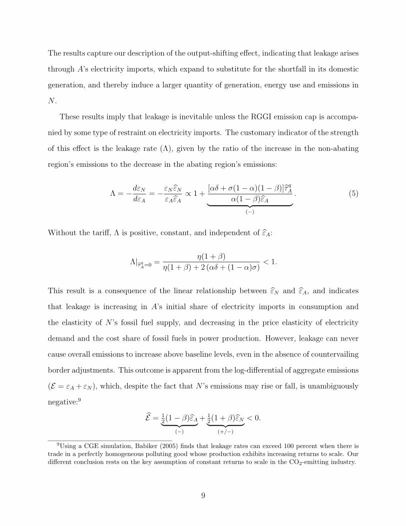
These results imply that leakage is inevitable unless the RGGI emission cap is accompa-

nied by some type of restraint on electricity imports. The customary indicator of the strength

of this effect is the leakage rate (Λ), given by the ratio of the increase in the non-abating

region’s emissions to the decrease in the abating region’s emissions:

Λ = −dεN

dεA

= −εN εN

εAεA

∝ 1 +[αδ + σ(1− α)(1− β)]τ q

A

α(1− β)εA︸ ︷︷ ︸(−)

. (5)

Without the tariff, Λ is positive, constant, and independent of εA:

Λ|bτqA=0 =

η(1 + β)

η(1 + β) + 2 (αδ + (1− α)σ)< 1.

This result is a consequence of the linear relationship between εN and εA, and indicates

that leakage is increasing in A’s initial share of electricity imports in consumption and

the elasticity of N ’s fossil fuel supply, and decreasing in the price elasticity of electricity

demand and the cost share of fossil fuels in power production. However, leakage can never

cause overall emissions to increase above baseline levels, even in the absence of countervailing

border adjustments. This outcome is apparent from the log-differential of aggregate emissions

(E = εA + εN), which, despite the fact that N ’s emissions may rise or fall, is unambiguously

negative:9

E = 12(1− β)εA︸ ︷︷ ︸

(−)

+ 12(1 + β)εN︸ ︷︷ ︸

(+/−)

< 0.

9Using a CGE simulation, Babiker (2005) finds that leakage rates can exceed 100 percent when there istrade in a perfectly homogeneous polluting good whose production exhibits increasing returns to scale. Ourdifferent conclusion rests on the key assumption of constant returns to scale in the CO2-emitting industry.

9

Turning to the impact of border adjustments, the tariff limits leakage by stimulating

import substitution via an increase in A’s domestic electricity supply, while simultaneously

attenuating demand. Table 2(a) is inconclusive as to whether the elasticities of the variables

with respect to the limit are smaller than those with respect to the tariff, whether the

results are more sensitive to the latter depends on the values of the parameters. Even so, Λ

is decreasing in the tariff, which completely neutralizes leakage if

τ qA,0 = − α(1− β)

αδ + σ(1− α)(1− β)εA > 0. (6)

For a given emission limit, the zero-leakage level of the tariff is increasing in the elasticity of

electricity demand, and decreasing in both A’s electricity import intensity as well as power

generator’s fossil fuel cost share and elasticity of substitution. The implication is that for

any value of εA, a sufficiently high electricity tariff can reverse leakage by limiting demand

for N ’s exports to the point where its production shrinks, inducing de facto reductions in

emissions.

Lastly, we consider the effect of the cap on the emission intensity of generation, which

falls in both regions in response to the emission limit.10 The additional influence of the tariff

is to amplify A’s intensity decline by stimulating its generators to produce more electricity

(implicitly, by substituting larger amounts of the clean generic factor for dirty carbon energy),

and attenuate N ’s intensity decline by inhibiting the export supply response of its power

sector.

To gain insight into RGGI’s impacts we use develop preliminary numerical estimates

based on the foregoing results. We parameterize the model by setting α = 0.3 (NEA/IEA,

2005), β = 3% and ε = −7.6% (following the statistics in Table 1), and assuming elasticity

values that are broadly consistent with the empirical literature: δ = 0.5, η = 1 and σ = 0.8.

Our findings, summarized in Table 2(b), indicate that RGGI’s environmental impact is likely

to be small. In the absence of border adjustments the price of carbon-energy in both regions

10A and N experience identical declines, which is an artifact of the model’s simplifying assumptions.

10

rises by 3%, and the quantity of carbon-energy used by the unconstrained region rises by

the same amount. A’s electricity output declines by 5.9% while N ’s output rises by 4.7%,

precipitating a neligible increase in power prices. Even so, electricity trade increases by

more than one and a half times, resulting in a leakage rate of 42% and a decline in aggregate

emissions of just over 2%. The zero-leakage electricity tariff implied by eq. (6) is small: 3.2%.

Imposing this tax on A’s electricity output generates a larger increase in the carbon-energy

price (10.7%), a smaller decline in power output (1.7%) and a more than 50% increase in

aggregate abatement.

Further insights can be obtained by looking at the consequences of imposing the no-

leakage electricity tariff on A in the absence of an emission target. The analytical solution

to the tax-only model is uninformative,11 but applying the parameter values above yields

the results in the last column of Table 2(b). Consistent with the elasticities in part (a) of

the table, the tax pushes electric power production, and the price and quantity of carbon-

energy inputs, upward in A and downward in N . Regions’ emission intensities respond

in the opposite manner due to the more elastic response of electricity output to the tax.

The price of electricity declines slightly while trade is sharply curtailed, resulting in 100%

leakage and unchanged overall emissions. This outcome suggests that, by itself, a tax on the

emission-intensive good cannot reduce overall pollution because of the increased production

stimulated by import substitution, and with it, demand for emission precursors. The key to

the improvement in environmental performance is therefore the joint impact of the tariff’s

attenuation of production and emissions in the exporting region in conjunction with the

emission limit’s restraint on the additional pollution induced by import substitution.

We conclude this section by noting the caveats to our findings thus far. First, the

prediction that RGGI’s effect on the emission intensity of generation will be everywhere

the same is an artifact of the two regions’ identical market size and fuel mix. Relaxing

these assumptions would certainly afford a more realistic characterization of RGGI’s impact,

11The complete results are available from the authors upon request.

11

but at a cost of much greater algebraic complexity.12 A second, related issue is that our

analytical model is incomplete because it ignores the rebound effect. Taking account of this

phenomenon would likely amplify the positive response of unconstrained states’ emission

intensities to abatement in RGGI states. Most importantly, the model’s narrow focus on

electric power also belies the fact that RGGI’s influence on the relative price of electricity

vis-a-vis fossil fuels will likely induce interfuel and energy-material substitution responses in

other sectors of the economy, whose net impact cannot be precisely forecast. If the rise in

electricity prices which attends the expansion of generation in unconstrained states results in

substitution of material inputs for energy, then the leakage to non-electric sectors will likely

be small. Conversely, leakage is likely to be large if the dominant response is substitution of

CO2-intensive fossil fuels for clean electricity.

Incorporating these factors into our analysis necessitates the use of a more detailed com-

putational model, to which we now turn.

3 The ICGE Model

3.1 Model structure

We employ an updated version of the ICGE model introduced by Sue Wing (2007). The

model is a static spatial price equilibrium simulation which divides the U.S. economy into 50

states and the District of Columbia (indexed by s = 1, . . . , S), and ten profit-maximizing

industry sectors (indexed by j = 1, . . . , N). The model’s sectoral disaggregation is

shown in Table 3. Each sector produces a single homogeneous commodity, indexed by

i = 1, . . . , N, and the set of commodities is partitioned into non-energy material goods

(m) and energy goods (e), a subset of which is associated with emissions of CO2.

In each industry and state, firms produce output (yj,s) from capital (kj,s), labor (lj,s)

12Regionally distinguishing the trade weights (βA = t/(qA + t) < βN = t/(qN − t) ∈ (0, 1)) and carbon-energy shares (αA < αN ) generates a complicated analytical solution which defies simple interpretation.

12

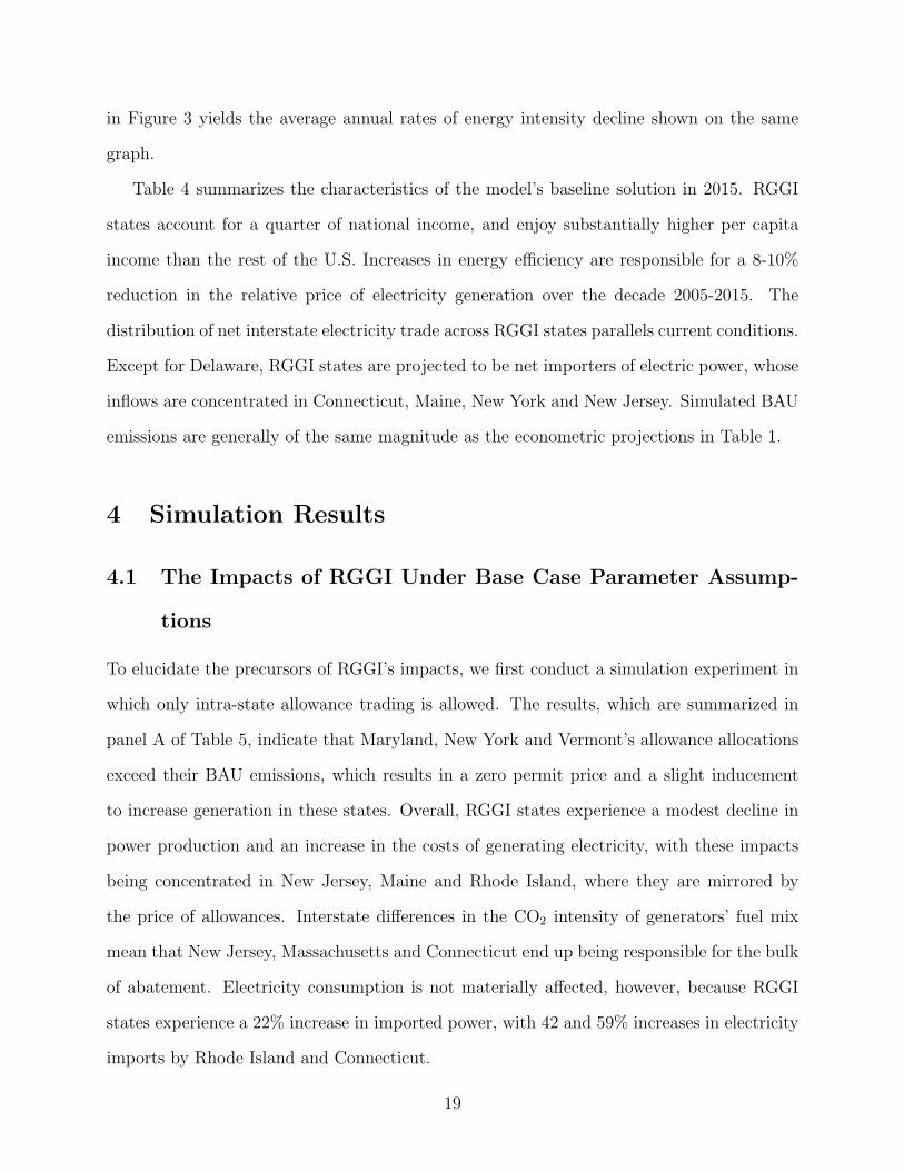
and an N -vector of intermediate inputs (xi,j,s), according to the simple bi-level production

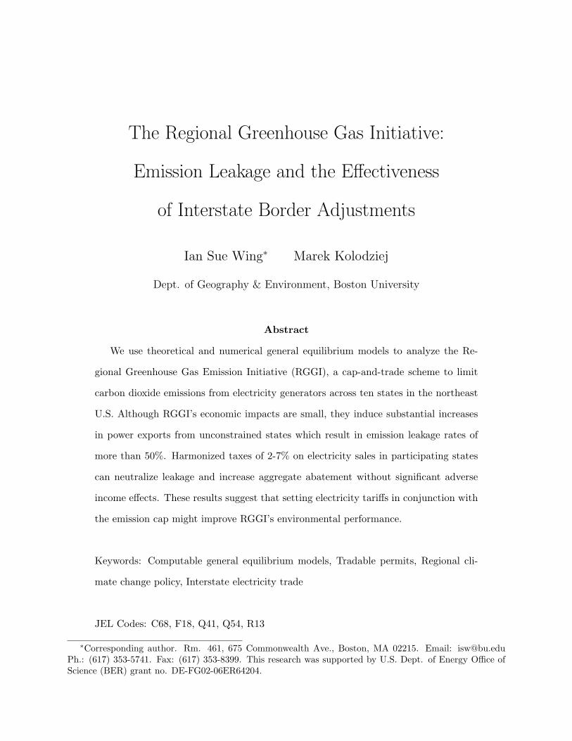
function shown schematically in Figure 1(a). Each node of the tree represents the output of a

sub-production function, the inputs to which are represented by the branches. Thus, output

is a Leontief function of three inputs: a CES aggregate of energy intermediate goods, a CES

aggregate of non-energy intermediate goods, and a Cobb-Douglas value-added composite of

capital and labor. The dual of output is the producer price (pj,s), defined as the unit cost of

production gross of taxes on output.

Households in each state are modeled as a utility-maximizing representative agent with

CES preferences over her consumption of commodities (ci,s). Consumption is financed out

of the income which each state agent receives from the rental of her endowments of labor

(Ls) and capital (Ks) to industries. To proxy for the interactions between the price system

and international trade in commodities, each state agent is endowed with a quantity of net

exports of goods and services (ni,s), which for simplicity is kept fixed throughout the analysis.

Interstate trade is modeled very simply, using the Armington (1969) assumption. Aggre-

gate supply of the ith good (Yi) is specified as an Armington CES composite of the 51 state

varieties. Consequently, the demands for each commodity by industries and households in all

states are fulfilled at a single, national market-clearing price (Pi) which is a weighted average

of the s state-level producer prices. In terms of the leakage problem, a key limitation of this

construct is its inability to represent the constraint of transmission capacity on bulk power

flows. To capture the balance between this effect and the fluid character of electric power

as a traded commodity, the base-case value of the Armington elasticity of substitution for

electricity was set at 4. As we go on to show, large variations in this parameter had only a

slight impact on the simulation results.

The model captures the imperfect mobility of factors across states and among industries

through the use of transformation functions which are shown schematically in Figure 1(b).

Imperfect factor mobility creates a divergence between each state’s total demand for labor

and capital and its corresponding endowments (Ls and Ks, respectively), so that Ls 6=∑

j lj,s

13

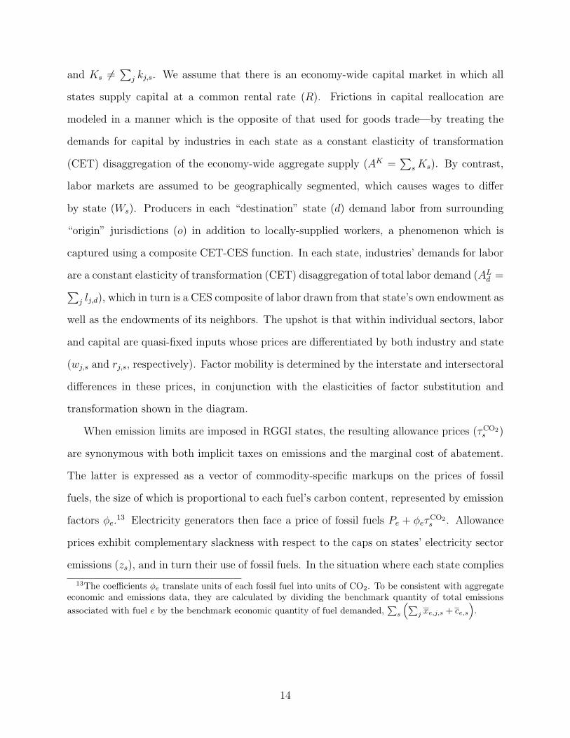
and Ks 6=∑

j kj,s. We assume that there is an economy-wide capital market in which all

states supply capital at a common rental rate (R). Frictions in capital reallocation are

modeled in a manner which is the opposite of that used for goods trade—by treating the

demands for capital by industries in each state as a constant elasticity of transformation

(CET) disaggregation of the economy-wide aggregate supply (AK =∑

sKs). By contrast,

labor markets are assumed to be geographically segmented, which causes wages to differ

by state (Ws). Producers in each “destination” state (d) demand labor from surrounding

“origin” jurisdictions (o) in addition to locally-supplied workers, a phenomenon which is

captured using a composite CET-CES function. In each state, industries’ demands for labor

are a constant elasticity of transformation (CET) disaggregation of total labor demand (ALd =∑

j lj,d), which in turn is a CES composite of labor drawn from that state’s own endowment as

well as the endowments of its neighbors. The upshot is that within individual sectors, labor

and capital are quasi-fixed inputs whose prices are differentiated by both industry and state

(wj,s and rj,s, respectively). Factor mobility is determined by the interstate and intersectoral

differences in these prices, in conjunction with the elasticities of factor substitution and

transformation shown in the diagram.

When emission limits are imposed in RGGI states, the resulting allowance prices (τCO2s )

are synonymous with both implicit taxes on emissions and the marginal cost of abatement.

The latter is expressed as a vector of commodity-specific markups on the prices of fossil

fuels, the size of which is proportional to each fuel’s carbon content, represented by emission

factors φe.13 Electricity generators then face a price of fossil fuels Pe + φeτ

CO2s . Allowance

prices exhibit complementary slackness with respect to the caps on states’ electricity sector

emissions (zs), and in turn their use of fossil fuels. In the situation where each state complies

13The coefficients φe translate units of each fossil fuel into units of CO2. To be consistent with aggregateeconomic and emissions data, they are calculated by dividing the benchmark quantity of total emissionsassociated with fuel e by the benchmark economic quantity of fuel demanded,

∑s

(∑j xe,j,s + ce,s

).

14

with its own target in autarkic fashion, we write this symbolically as

εs ≤ zs ⊥ τCO2s , s ∈ RGGI,

where εs =∑

e φexe,Ele.,s is the CO2 emitted in the course of the electric power sector’s

combustion of each type of fossil fuel. This expression represents intra-state emission trading,

where generators in a particular state trade allowances only amongst themselves to equalize

their marginal costs of CO2 control. To simulate interstate emission trading we solve the

model for the common market-clearing price of permits across states (τCO2s = τCO2) which

is consistent with the aggregate RGGI cap, Z =∑

s∈RGGI zs:

∑s∈RGGI

εs ≤ Z ⊥ τCO2 .

Now, generators across RGGI states choose their levels of emissions optimally by setting their

marginal cost of abatement equal to common market-clearing price of allowances, whose value

is determined by the difference between Z and the business as usual (BAU) emission level.

The geographic pattern of welfare impacts depends on states’ allowance allocations, zs,

given in Table 1. This may be seen by examining the definition of annual state personal

income (ASPI) in the model:

ASPIs = (WsLs +RKs) + TRSs + FEs +NFAs ∀s

+

τCO2s εs Intra-state Permit Trade

τCO2(zs − εs) Interstate Permit Trades ∈ RGGI

+ τEle.PEle.

(cEle.,s +

∑j

xEle.,j,s

)s ∈ RGGI (7)

Here, FEs denotes federal government expenditures within each state, which indicate each

state’s receipts of recycled revenue from federal labor, capital and production taxes. The

15

variable TRSs denotes recycled revenue from state labor, capital and production taxes,

NFAs =∑

i Pini,s indicates each state’s net foreign asset position, and the term in paren-

theses is each state’s factor income.14

The last two terms in eq. (7) represent the impacts of CO2 allowance trading and

recycled revenue from electricity tariffs. In the model, grandfathering of allowances to firms is

equivalent to defining a new factor of production which is owned by households, the returns to

which redound to each state representative agent. Auctioning allowances generates additional

revenue to state governments which is then recycled to the corresponding representative

agent. In both cases the simulated income effects are the same. With intra-state allowance

trading the electric power sector is assumed to just comply with its emission target (εs = zs).

With interstate trading, if a state over-complies with its abatement target, or is allocated

allowances in excess of its BAU level of emissions, its revenue rises due to permit sales.

Conversely, a state which emits CO2 in excess of its allocation will find it necessary to

purchase allowances to stay in compliance, and will see its income decrease.

For transparency we represent border measures in the same way as our theoretical model.

Our simple assumption is that RGGI states levy harmonized tariffs (τ ele.) on electricity

consumed within their borders, which allows us to boil the effects of more complicated

schemes described in Farnsworth et al. (2007) down to a single metric—the RGGI-wide

premium on the consumer price of electricity. Doing so allows us to search over values of

this instrument to find the level of the tariff which just neutralizes the sum of internal and

external leakage. An algebraic summary of the model is given in an appendix to the paper.

One final point bears mentioning. Because of the pre-existing distortionary taxes in the

no-abatement equilibrium, the ultimate welfare impact in a given state depends on adverse

effect of the primary burden of that jurisdiction’s abatement on factor returns on one hand,

14The model is closed by imposing budgetary balance at the federal level∑

s FEs =∑

s TRFs where TRF

s

is the revenue from the sum of federal taxes on labor, capital and production raised in each state. The basisfor our closure rule is the assumption that the pattern of federal spending is invariant to climate policy, sothat the ratio $s = FEs/

∑s FEs remains the same, with or without RGGI. The value of $s is set equal

to the state share of federal government spending in the benchmark dataset used to calibrate the model.

16

and benefits of recycled funds from pre-existing taxes, allowance allocations, and electricity

tariffs on the other. We shall see that with policies such as RGGI which bind lightly on the

economy, the first effect is sufficiently small that it is dominated by the second. The theory

of the second best is the key to this result, as the general equilibrium effects of distorting

production decisions in an initially tariff-ridden economy give rise to a net welfare gain.

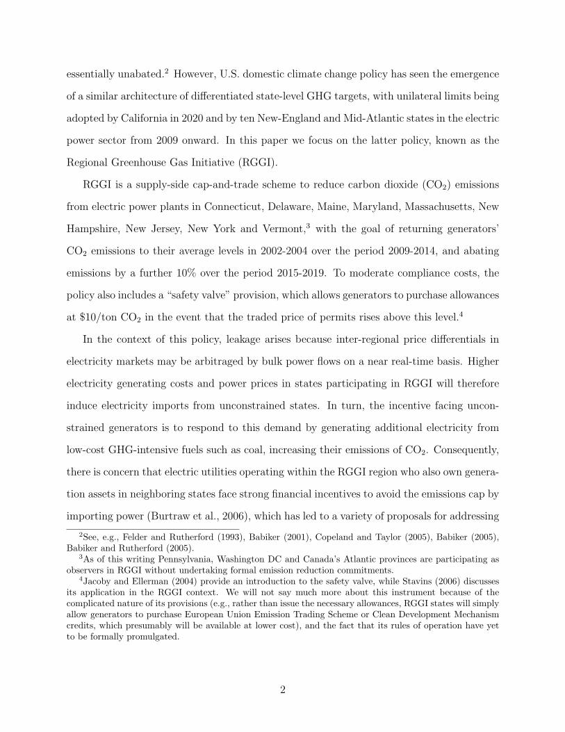
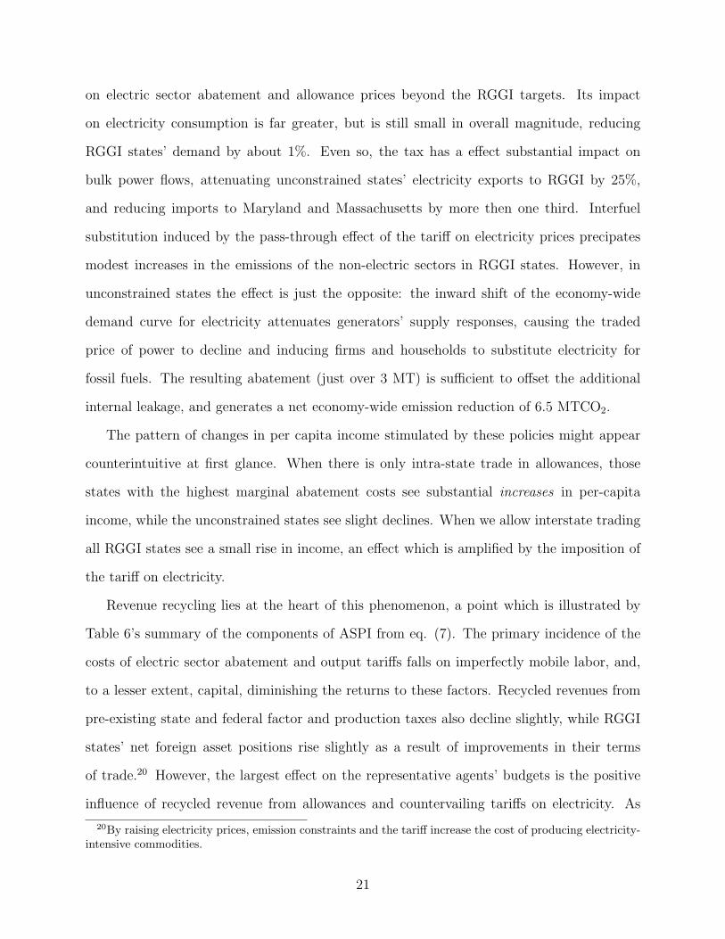
3.2 Data, Parameters and Calibration

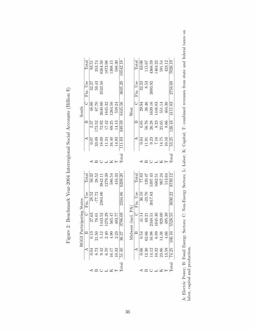
The model was calibrated on an inter-regional social accounting matrix (SAM) constructed

from Bureau of Labor Statistics (BLS) nominal input-output data for the aggregate U.S.

economy in 2004. Intermediate energy uses were adjusted using statistics from the Energy

Information Administration’s (EIA) Electric Power Annual. The resulting aggregate SAM

was regionalized using Bureau of Economic Analysis (BEA) data on the components of state

GDP and annual state personal income, as well as information on state energy consumption

by fuel and sector from EIA’s State Energy Data System. States’ benchmark labor endow-

ments were imputed using Journey to Work data from the 2000 Census, which allowed us

to estimate benchmark capital earnings as residual value-added after taxes. We calibrated

benchmark state and federal tax burdens by industry, as well as interstate revenue flows us-

ing data on state and federal tax revenues and expenditures from the Census Consolidated

Federal Funds Report, Internal Revenue Service Databooks and supplemental state data

files.15 The final benchmark dataset is shown in Figure 2.

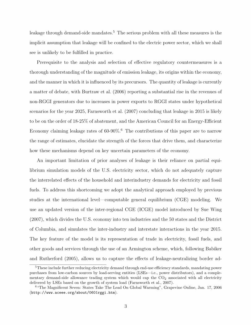
We construct our base-case projection of the economy in 2015 by scaling each state’s

benchmark endowments of labor and capital according to the historical average annual

growth rates of state GDP, shown in Figure 3. To project BAU CO2 emissions we eschew

the customary use of a secular autonomous energy efficiency improvement (AEEI) factor to

down-scale the coefficient on energy in the model’s cost and expenditure functions (θe,j,s and

αe,s).16 Instead, we base our approach on Metcalf’s (2007) recent finding that the growth of

15The procedures employed are described in detail by Sue Wing (2007).16For discussion see, e.g., Sue Wing and Eckaus (2007).

17

states’ incomes induces substantial declines in their energy-GDP ratios. We econometrically

estimate the long-run income elasticity of energy intensity (Ω), which we use to compute

state-specific average rates of energy intensity decline as a function of the growth of states’

GDP. Our final step is to replace the AEEI index by compounding these declines into an

energy-intensity scale factor, which we then use to down-scale θe,j,s and αe,s.

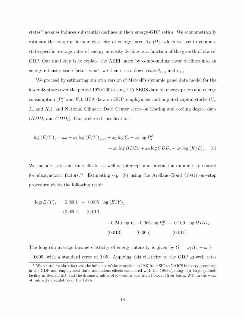
We proceed by estimating our own version of Metcalf’s dynamic panel data model for the

lower 48 states over the period 1970-2004 using EIA SEDS data on energy prices and energy

consumption (PEs and Es), BEA data on GDP, employment and imputed capital stocks (Ys,

Ls and Ks), and National Climatic Data Center series on heating and cooling degree days

(HDDs and CDDs). Our preferred specification is:

log (E/Y )s = ω0 + ω1 log (E/Y )s,−1 + ω2 log Ys + ω3 logPEs

+ ω4 logHDDs + ω5 logCDDs + ω6 log (K/L)s . (8)

We include state and time effects, as well as intercept and interaction dummies to control

for idiosyncratic factors.17 Estimating eq. (8) using the Arellano-Bond (1991) one-step

procedure yields the following result:

log(E/Y )s = 0.0001 + 0.605 log (E/Y )s,−1

(0.0004) (0.016)

−0.240 log Ys −0.066 logPEs + 0.109 logHDDs.

(0.013) (0.005) (0.011)

The long-run average income elasticity of energy intensity is given by Ω = ω2/(1 − ω1) =

−0.605, with a standard error of 0.05. Applying this elasticity to the GDP growth rates

17We control for three factors: the influence of the transition in 1997 from SIC to NAICS industry groupingsin the GDP and employment data, anomalous effects associated with the 1984 opening of a large synfuelsfacility in Beulah, SD, and the dramatic influx of low-sulfur coal from Powder River basin, WY, in the wakeof railroad deregulation in the 1980s.

18

in Figure 3 yields the average annual rates of energy intensity decline shown on the same

graph.

Table 4 summarizes the characteristics of the model’s baseline solution in 2015. RGGI

states account for a quarter of national income, and enjoy substantially higher per capita

income than the rest of the U.S. Increases in energy efficiency are responsible for a 8-10%

reduction in the relative price of electricity generation over the decade 2005-2015. The

distribution of net interstate electricity trade across RGGI states parallels current conditions.

Except for Delaware, RGGI states are projected to be net importers of electric power, whose

inflows are concentrated in Connecticut, Maine, New York and New Jersey. Simulated BAU

emissions are generally of the same magnitude as the econometric projections in Table 1.

4 Simulation Results

4.1 The Impacts of RGGI Under Base Case Parameter Assump-

tions

To elucidate the precursors of RGGI’s impacts, we first conduct a simulation experiment in

which only intra-state allowance trading is allowed. The results, which are summarized in

panel A of Table 5, indicate that Maryland, New York and Vermont’s allowance allocations

exceed their BAU emissions, which results in a zero permit price and a slight inducement

to increase generation in these states. Overall, RGGI states experience a modest decline in

power production and an increase in the costs of generating electricity, with these impacts

being concentrated in New Jersey, Maine and Rhode Island, where they are mirrored by

the price of allowances. Interstate differences in the CO2 intensity of generators’ fuel mix

mean that New Jersey, Massachusetts and Connecticut end up being responsible for the bulk

of abatement. Electricity consumption is not materially affected, however, because RGGI

states experience a 22% increase in imported power, with 42 and 59% increases in electricity

imports by Rhode Island and Connecticut.

19

The RGGI caps reduce electric sector emissions by 17 MTCO2, but half this amount is

offset by increased emissions from outside RGGI—more than 8 MT from electric power and

just under 3 MT from other industries.18 As well, within RGGI, substitution of fossil fuels

for electricity as the latter’s price increases generates just under 1 MT of internal leakage.

These results imply a net abatement of just under 5 MTCO2, with an overall leakage rate of

71%.

Panel B summarizes the different set of impacts which arise when trade in allowances

is permitted among generators in different states. Electricity consumption is virtually un-

changed, and there is only a slight increase in the cost and attenuation in the quantity of

electric power production. The expansion of electricity trade is also much smaller than oc-

curs under autarkic state compliance, and is concentrated in Connecticut and New York.

Allowance prices are in the $2-3/ton range (in agreement with Farnsworth et al., 2007, p. 5)

and abatement activity is less vigorous and more evenly distributed among the states. The

reason is of course that Maryland, New York and Vermont sell their excess allowances, which

then play the role of “hot air” in the trading system, relaxing the aggregate emission con-

straint by 10 MT. The consequent smaller increase in generation costs results in less leakage:

3.2 MT, relative to a base of 6.5 MT of gross electric sector CO2 abatement. However, this

still translates into a leakage rate of approximately 50%, which, although an improvement

over intra-state allowance trading, comes at the cost of lower net abatement (3.3 MT).19

Not surprisingly, the level of the harmonized tariff required to neutralize leakage is quite

low (2.5%), echoing the results of Section 2. As indicated in panel C, the tax imposes a slight

additional adverse effect on electricity production, but has a neglibible additional impact

18The Armington trade structure does not permit us to pinpoint the origins of the additional electric powerconsumed by RGGI states, or the precise quantity of emissions associated therewith (i.e., separate from theconfounding effects of general equilibrium adjustments in fuel markets). Nevertheless, in the simulationresults Texas, Florida and Pennsylvania experience the largest expansion of electric generation.

19This figure represents 3.5% of baseline electric sector emissions (in excellent agreement with our theo-retical model), but only 0.4% of the CO2 emitted by RGGI states and 0.05% of aggregate U.S. emissions.Moreover, the ICGE model’s Armington trade structure, general equilibrium interactions, and ability to ac-count for the fact that RGGI states make up less than 15% of aggregate electricity consumption give rise toa modest increase in electricity trade (3.3%), a far cry from the more dramatic predictions of the theoreticalmodel.

20

on electric sector abatement and allowance prices beyond the RGGI targets. Its impact

on electricity consumption is far greater, but is still small in overall magnitude, reducing

RGGI states’ demand by about 1%. Even so, the tax has a effect substantial impact on

bulk power flows, attenuating unconstrained states’ electricity exports to RGGI by 25%,

and reducing imports to Maryland and Massachusetts by more then one third. Interfuel

substitution induced by the pass-through effect of the tariff on electricity prices precipates

modest increases in the emissions of the non-electric sectors in RGGI states. However, in

unconstrained states the effect is just the opposite: the inward shift of the economy-wide

demand curve for electricity attenuates generators’ supply responses, causing the traded

price of power to decline and inducing firms and households to substitute electricity for

fossil fuels. The resulting abatement (just over 3 MT) is sufficient to offset the additional

internal leakage, and generates a net economy-wide emission reduction of 6.5 MTCO2.

The pattern of changes in per capita income stimulated by these policies might appear

counterintuitive at first glance. When there is only intra-state trade in allowances, those

states with the highest marginal abatement costs see substantial increases in per-capita

income, while the unconstrained states see slight declines. When we allow interstate trading

all RGGI states see a small rise in income, an effect which is amplified by the imposition of

the tariff on electricity.

Revenue recycling lies at the heart of this phenomenon, a point which is illustrated by

Table 6’s summary of the components of ASPI from eq. (7). The primary incidence of the

costs of electric sector abatement and output tariffs falls on imperfectly mobile labor, and,

to a lesser extent, capital, diminishing the returns to these factors. Recycled revenues from

pre-existing state and federal factor and production taxes also decline slightly, while RGGI

states’ net foreign asset positions rise slightly as a result of improvements in their terms

of trade.20 However, the largest effect on the representative agents’ budgets is the positive

influence of recycled revenue from allowances and countervailing tariffs on electricity. As

20By raising electricity prices, emission constraints and the tariff increase the cost of producing electricity-intensive commodities.

21

alluded to above, this is a second-best result which arises because the RGGI emission targets

bind lightly on their respective economies, which has a small distortionary impact that is

easily mitigated by the additional income from recycled revenue. Similar gains in net income

would likely not be experienced with more stringent targets that require substantial emission

reductions and incur significant abatement costs.

4.2 Sensitivity Analysis

We now investigate the robustness of our findings to key uncertain economic processes rep-

resented by the model parameters. Specifically, we examine the influence of four factors: the

assumed rates of state energy intensity decline, our projections of future economic growth

based on recent trends in state GDP, and the assumed values for interfuel and interstate

Armington energy elasticities of substitution. We proceed by perturbing each of the relevant

parameters in a sequential fashion. The results are shown in Table 7. For each set of pa-

rameter changes we also run the model with the computed value of the leakage-neutralizing

RGGI tariff, and summarize the results in Table 8.

Our base case (A) assumes default values for the income elasticity of energy intensity (Ω

= -0.606), the interfuel elasticity of substitution (σE =0.7) and the Armington elasticities

of substitution representing interstate trade in fossil fuels (σACoal, σ

ACrude Oil/Gas, σ

AGas = 0.8;

σAPetroleum = 1.4) and electricity (σA

Ele. = 4). Case B tests the impact of uncertainty in the

evolution of state energy intensity, first by varying Ω by ± 2 standard deviations relative

to its mean (-0.71 and -0.51), and second by directly imposing slower growth rates for the

energy-GDP ratio (1% and 0.5% p.a.) which understate historical trends but lie in the

range of values of the AEEI parameter routinely employed by CGE models (Sue Wing and

Eckaus, 2007). Case C examines the impact of our economic growth projections by varying

the projected rates of growth of states’ GDP in Figure 3 by ±1 standard deviation relative

to their respective means. Cases D and E examine the influence of our choice of substitution

elasticities, testing the substitutability among fuels in production and among geographic

22

sources of electricity and fossil fuels (respectively) by doubling and halving σE and σA.

The impact of these parameters in order of increasing influence is as follows: Armington

elasticities, interfuel substitution elasticities, economic growth and energy-intensity decline.

The Armington elasticities of substitution have an negligibly small impact on the simulation

results. The interfuel elasticity of substitution has a nonlinear effect—abatement and leakage

rise when σE is doubled as well as when it is halved, with the latter effect being very slight.

In contrast with the predictions of our analytical model, when the rebound effect is ac-

counted for, the aggregate emission intensity of electricity generation declines significantly

within RGGI while rising slightly in unconstrained states. Except for the 0.5% and 1% AEEI

cases where energy intensity declines more slowly than in the past—which would likely trigger

RGGI’s safety valve provision—aggregate electricity prices turn out to be largely unaffected

by RGGI. Nonetheless, abating states increase their net imports of electric power, which,

out of all the variables we examine, ends up being the most sensitive to variations in the

parameters. The consequence for CO2 abatement is that RGGI generators make modest

emission reductions which are largely unaffected by internal leakage, slightly attenuated by

the expansion of generation in unconstrained states, and substantially offset by interfuel

substitution in non-electric industries outside the RGGI region. The result is that net aggre-

gate emission reductions range from 0.5-24 MT, with corresponding leakage rates of 47-57%.

Allowance prices are generally in the $2-10 range, and recycled permit revenues, combined

with the caps’ small primary abatement burden, lead to slight increases in RGGI states’

average per capita income.

Table 8 illustrates that the foregoing picture changes significantly once electricity taxes

are imposed. The tariffs necessary to neutralize leakage are generally modest, in the range

of 2-7% of the BAU electricity price. The combined costs of electricity taxes and emission

abatement lead to higher power prices within RGGI states, which induce reductions in

electricity demand and imports that are sufficiently large that the aggregate Armington

electricity price experiences a slight decline, indicating an inward shift in the aggregate

23

electricity demand curve. The emission intensity of RGGI generators remains the same, but

that of power producers in unconstrained states now falls instead of expanding. Electric

sector CO2 abatement and allowance prices in RGGI are unaffected, but the overall cuts

in emissions made by RGGI states are much smaller because their non-electric industries

substitute away from more costly electricity toward now-cheaper toward fossil fuel inputs.

The latter effect is more pronounced in RGGI states, but is offset by the dramatic reversal

in the sign of leakage in the electricity sector in unconstrained states, where the attenuating

effect of the tariff on exports of electricity to RGGI states induces generators to reduce their

output, fossil fuel use, and emissions. Finally, the income effects of the cap-and-trade scheme

and the tax and are twice as large those without the tax, as the tariff’s beneficial revenue

recycling effect outweighs its distortionary effect on factor returns. Notwithstanding this,

the economic impact on RGGI states remains small.

5 Summary and concluding remarks

We have used a analytical and numerical models to analyze the economic and environmental

impacts of the Regional Greenhouse Gas Initiative. Both of these effects are small due to the

generous allocation of CO2 emission allowances to electricity generators under RGGI’s cap-

and-trade system. The initiative’s environmental effectiveness is further diminished by the

ability of consumers within RGGI to import electricity from states not subject to emission

limits, increasing the likelihood of larger inflows of bulk power and with them substantial

leakage of emissions. Simulations indicate that 49-57% of the CO2 abated by RGGI electric

generators will be offset by unconstrained sources, with two-thirds of these emissions coming

from the expansion of power production and export by generators in non-RGGI states, and

the remainder from increases in the demand for fossil fuels by non-electric industries both

outside and—to a lesser extent—inside of the RGGI umbrella.

More optimistically, we find that border measures—which we have modeled simply as

24

harmonized tariffs on electricity consumed in RGGI states—can be an effective instrument

to neutralize leakage when used in conjunction with a cap-and-trade system. Our numerical

results show that taxes of 2-7% on electricity depress RGGI states’ demand for power and

cause an inward shift in the aggregate U.S. demand curve for electric power, which simulta-

neously attenuates the export response of generators in unconstrained states, reduces power

prices, and induces household and industrial energy consumers to substitute electricity for

fossil fuels. This last effect is dominant in unconstrained states, where its magnitude is large

enough to offset the impact of the reverse (i.e., fossil fuel for electricity) substitution effect

in RGGI’s non-electric sectors as a result of higher power prices there. The upshot is that

while cap on CO2 induces RGGI states to export emissions to unconstrained counterparts,

harmonized tariffs have the opposite effect of inducing exports of abatement, which can be

thought of as “negative” or “reverse” leakage.

A key contribution of this paper has been to highlight the feedback mechanism whereby

electricity taxes affect interfuel substitution in non-electric sectors, an effect which makes a

sizable contribution to the overall quantity of emission leakage. But, as with any simulation

study, our results are sensitive to the parameter values and structural assumptions of our

numerical model. Our sensitivity analysis is an attempt to shed light on the implications of

the former, but some aspects of the latter remain problematic, as we go on to elaborate.

Perhaps the most serious limitation of our ICGE model is the lack of data on state-to-

state electric power flows and the consequent use of an Armington structure to model trade

in electricity, which prevent us from simulating the effect of transmission constraints RGGI

states’ power imports. An attempt to capture the influence of these constraints by halving

the benchmark value of the Armington elasticity of substitution had a negligible impact on

the simulation results. However, given the admittedly heuristic character of this workaround,

we prefer to interpret our finding as the upper bound on the true magnitude of leakage.

Lack of data on the components of income at the state level gives rise to a further

shortcoming, namely, the inability of the model to distinguish between consumption and

25

investment. Our characterization of RGGI’s economic impacts is therefore restricted to

near-term income effects, and resolves neither short-run consumption-based welfare impacts

nor the influence of changes in investment on capital accumulation and long-run income

growth.

A third issue involves the simple production function used to characterize producer be-

havior, which in the electric power sector glosses over the response of different generation

technologies to the emission limit, particularly the inducement of renewables such as wind.

While the ability to explicitly represent the expansion of low-cost electricity supply options

within the model would likely lower our estimates of RGGI’s costs, it should be noted that

replacing a smooth production function with an array of discrete Leontief activities may have

the opposite effect because of the diminished substitutability among inputs to the sector as a

whole (Sue Wing, 2005). The implications for abatement costs and leakage therefore depend

on the relative importance of these two influences.

Finally, we have entirely sidestepped the issue of volatility in RGGI states’ baseline

emissions, and its implications for whether the cap binds. Over the decade 1995-2004 CO2

emitted by RGGI electric generators fluctuated markedly, so much so that the mean of

the annual growth rates of emissions was less than one third of their standard deviation! To

understand the sources of such volatility and their consequences for the expected magnitudes

of RGGI’s environmental and economic impacts, we would need to conduct a parametric

uncertainty analysis, which is a separate undertaking that is beyond the scope of the present

study.

The development of data and modeling techniques to address these issues is the focus of

ongoing research by the authors.

26

Appendix: Algebraic Summary of the Model (Can be

deleted in proof)

Prices

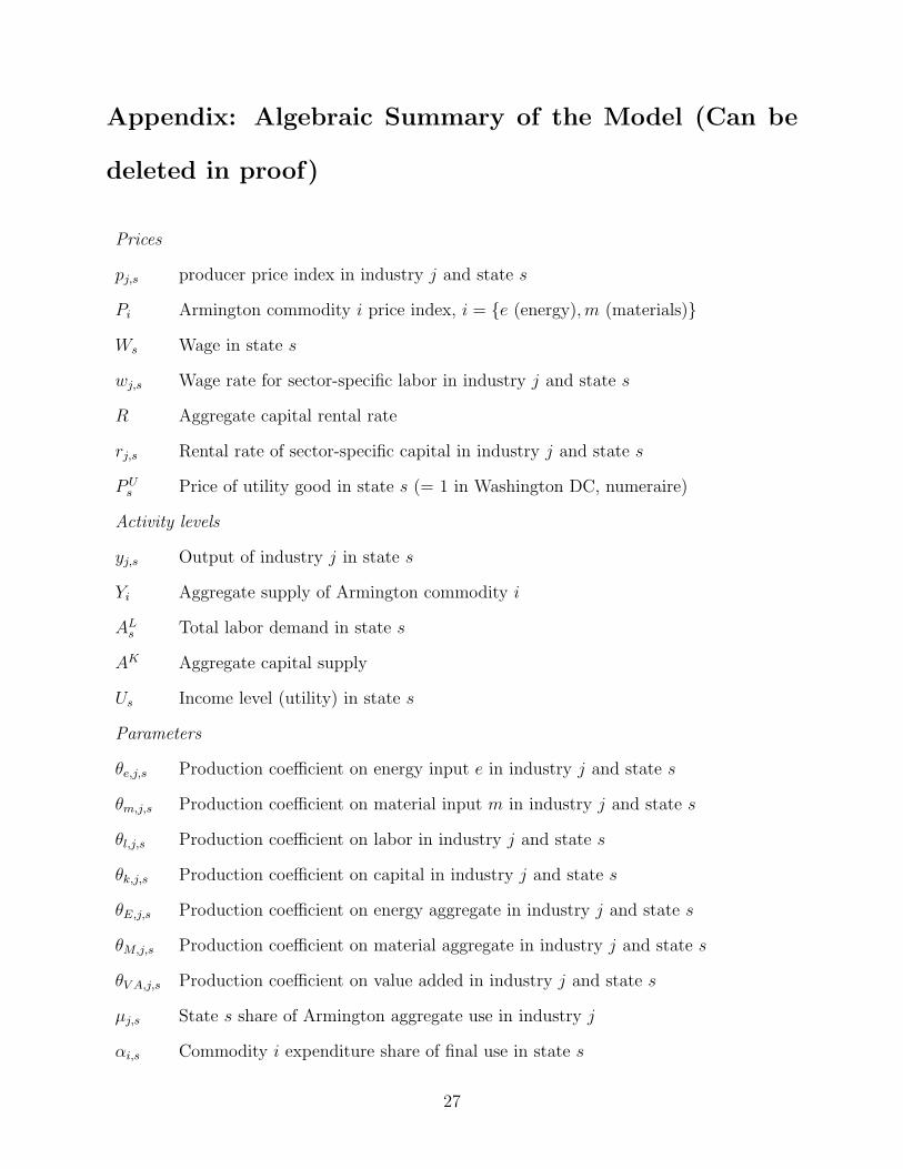
pj,s producer price index in industry j and state s

Pi Armington commodity i price index, i = e (energy),m (materials)

Ws Wage in state s

wj,s Wage rate for sector-specific labor in industry j and state s

R Aggregate capital rental rate

rj,s Rental rate of sector-specific capital in industry j and state s

PUs Price of utility good in state s (= 1 in Washington DC, numeraire)

Activity levels

yj,s Output of industry j in state s

Yi Aggregate supply of Armington commodity i

ALs Total labor demand in state s

AK Aggregate capital supply

Us Income level (utility) in state s

Parameters

θe,j,s Production coefficient on energy input e in industry j and state s

θm,j,s Production coefficient on material input m in industry j and state s

θl,j,s Production coefficient on labor in industry j and state s

θk,j,s Production coefficient on capital in industry j and state s

θE,j,s Production coefficient on energy aggregate in industry j and state s

θM,j,s Production coefficient on material aggregate in industry j and state s

θV A,j,s Production coefficient on value added in industry j and state s

µj,s State s share of Armington aggregate use in industry j

αi,s Commodity i expenditure share of final use in state s

27

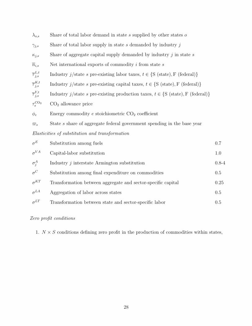
λo,s Share of total labor demand in state s supplied by other states o

γj,s Share of total labor supply in state s demanded by industry j

κj,s Share of aggregate capital supply demanded by industry j in state s

ni,s Net international exports of commodity i from state s

τL,tj,s Industry j/state s pre-existing labor taxes, t ∈ S (state),F (federal)

τK,tj,s Industry j/state s pre-existing capital taxes, t ∈ S (state),F (federal)

τY,tj,s Industry j/state s pre-existing production taxes, t ∈ S (state),F (federal)

τCO2s CO2 allowance price

φe Energy commodity e stoichiometric CO2 coefficient

$s State s share of aggregate federal government spending in the base year

Elasticities of substitution and transformation

σE Substitution among fuels 0.7

σV A Capital-labor substitution 1.0

σAj Industry j interstate Armington substitution 0.8-4

σC Substitution among final expenditure on commodities 0.5

σKT Transformation between aggregate and sector-specific capital 0.25

σLA Aggregation of labor across states 0.5

σLT Transformation between state and sector-specific labor 0.5

Zero profit conditions

1. N × S conditions defining zero profit in the production of commodities within states,

28

complementary to the N × S activity levels of industries within states:

pj,s = (1 + τY,Sj,s + τY,F

j,s )

×

1

θE,j,s

∑e6=Ele.

θσE

e,j,s(Pe + φeτCO2)1−σE

+ θσE

Ele.,j,s(PEle.(1 + τEle.))1−σE

1/(1−σE)

+1

θV A,j,s

(1 + τL,S

j,s + τL,Fj,s )wj,s

θL,j,s

(1 + τK,Sj,s + τK,F

j,s )rj,s

θK,j,s

+1

θM,j,s

∑m

Pm/θm,j,s

]⊥ yj,s, j = Ele., s ∈ RGGI

pj,s = (1 + τY,Sj,s + τY,F

j,s )

×

1

θE,j,s

∑e6=Ele.

θσE

e,j,sP1−σE

e + θσE

Ele.,j,s(PEle.(1 + τEle.))1−σE

1/(1−σE)

+1

θV A,j,s

(1 + τL,S

j,s + τL,Fj,s )wj,s

θL,j,s

(1 + τK,Sj,s + τK,F

j,s )rj,s

θK,j,s

+1

θM,j,s

∑m

Pm/θm,j,s

]⊥ yj,s, j 6= Ele., s ∈ RGGI

pj,s = (1 + τY,Sj,s + τY,F

j,s )

1

θE,j,s

∑e

θσE

e,j,sP1−σE

e

1/(1−σE)

+1

θV A,j,s

(1 + τL,S

j,s + τL,Fj,s )wj,s

θL,j,s

(1 + τK,Sj,s + τK,F

j,s )rj,s

θK,j,s

+1

θM,j,s

∑m

Pm/θm,j,s

]⊥ yj,s, s 6∈ RGGI (ZP1)

2. N conditions defining zero profit in interstate trade in commodities, complementary

to the N Armington aggregate commodity supply activity levels:

Pj =

(∑s

µσA

j

j,s p1−σA

j

j,s

)1/(1−σAj )

⊥ Yj (ZP2)

29

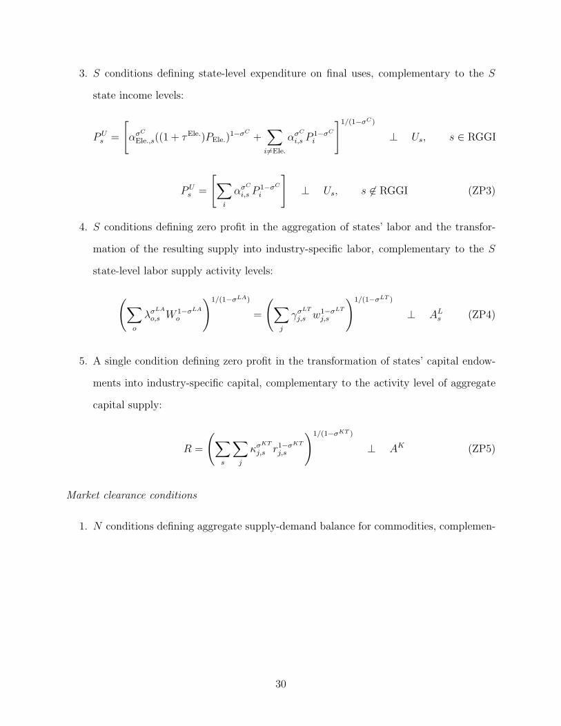
3. S conditions defining state-level expenditure on final uses, complementary to the S

state income levels:

PUs =

[ασC

Ele.,s((1 + τEle.)PEle.)1−σC

+∑

i6=Ele.

ασC

i,s P1−σC

i

]1/(1−σC)

⊥ Us, s ∈ RGGI

PUs =

[∑i

ασC

i,s P1−σC

i

]⊥ Us, s 6∈ RGGI (ZP3)

4. S conditions defining zero profit in the aggregation of states’ labor and the transfor-

mation of the resulting supply into industry-specific labor, complementary to the S

state-level labor supply activity levels:

(∑o

λσLA

o,s W 1−σLA

o

)1/(1−σLA)

=

(∑j

γσLT

j,s w1−σLT

j,s

)1/(1−σLT )

⊥ ALs (ZP4)

5. A single condition defining zero profit in the transformation of states’ capital endow-

ments into industry-specific capital, complementary to the activity level of aggregate

capital supply:

R =

(∑s

∑j

κσKT

j,s r1−σKT

j,s

)1/(1−σKT )

⊥ AK (ZP5)

Market clearance conditions

1. N conditions defining aggregate supply-demand balance for commodities, complemen-

30

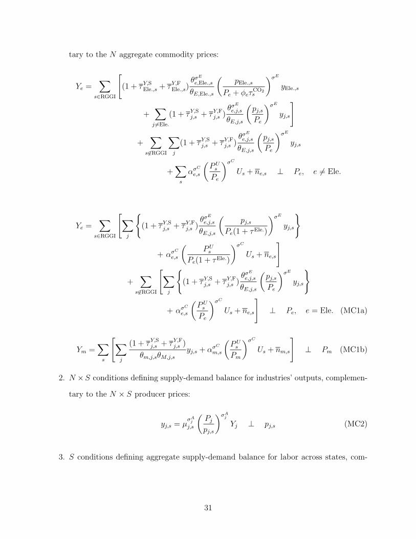
tary to the N aggregate commodity prices:

Ye =∑

s∈RGGI

[(1 + τY,S

Ele.,s + τY,FEle.,s)

θσE

e,Ele.,s

θE,Ele.,s

(pEle.,s

Pe + φeτCO2s

)σE

yEle.,s

+∑

j 6=Ele.

(1 + τY,Sj,s + τY,F

j,s )θσE

e,j,s

θE,j,s

(pj,s

Pe

)σE

yj,s

]

+∑

s 6∈RGGI

∑j

(1 + τY,Sj,s + τY,F

j,s )θσE

e,j,s

θE,j,s

(pj,s

Pe

)σE

yj,s

+∑

s

ασC

e,s

(PU

s

Pe

)σC

Us + ne,s ⊥ Pe, e 6= Ele.

Ye =∑

s∈RGGI

[∑j

(1 + τY,S

j,s + τY,Fj,s )

θσE

e,j,s

θE,j,s

(pj,s

Pe(1 + τEle.)

)σE

yj,s

+ ασC

e,s

(PU

s

Pe(1 + τEle.)

)σC

Us + ne,s

]

+∑

s 6∈RGGI

[∑j

(1 + τY,S

j,s + τY,Fj,s )

θσE

e,j,s

θE,j,s

(pj,s

Pe

)σE

yj,s

+ ασC

e,s

(PU

s

Pe

)σC

Us + ne,s

]⊥ Pe, e = Ele. (MC1a)

Ym =∑

s

[∑j

(1 + τY,Sj,s + τY,F

j,s )

θm,j,sθM,j,s

yj,s + ασC

m,s

(PU

s

Pm

)σC

Us + nm,s

]⊥ Pm (MC1b)

2. N ×S conditions defining supply-demand balance for industries’ outputs, complemen-

tary to the N × S producer prices:

yj,s = µσA

j

j,s

(Pj

pj,s

)σAj

Yj ⊥ pj,s (MC2)

3. S conditions defining aggregate supply-demand balance for labor across states, com-

31

plementary to the S average state wage levels:

Ls =∑

d

λσLA

s,d

(∑

o λσLA

o,d W 1−σLA

o

)1/(1−σLA)

Ws

σLA

ALd ⊥ Ws (MC3)

4. N×S conditions defining the supply-demand balance for industry-specific labor within

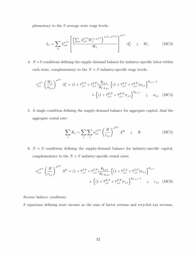
each state, complementary to the N × S industry-specific wage levels:

γσLT

j,s

(Ws

wj,s

)σLT

ALs = (1 + τY,S

j,s + τY,Fj,s )

θl,j,s

θV A,j,s

(1 + τL,S

j,s + τL,Fj,s )wj,s

θl,j,s−1

×

(1 + τK,Sj,s + τK,F

j,s )rj,s

θK,j,s

⊥ wj,s (MC4)

5. A single condition defining the supply-demand balance for aggregate capital, dual the

aggregate rental rate:

∑s

Ks =∑

j

∑s

κσKT

j,s

(R

rj,s

)σKT

AK ⊥ R (MC5)

6. N × S conditions defining the supply-demand balance for industry-specific capital,

complementary to the N × S industry-specific rental rates:

κσKT

j,s

(R

rj,s

)σKT

AK = (1 + τY,Sj,s + τY,F

j,s )θk,j,s

θV A,j,s

(1 + τL,S

j,s + τL,Fj,s )wj,s

θl,j,s

×

(1 + τK,Sj,s + τK,F

j,s )rj,s

θK,j,s−1

⊥ rj,s (MC6)

Income balance conditions

S equations defining state income as the sum of factor returns and recycled tax revenue,

32

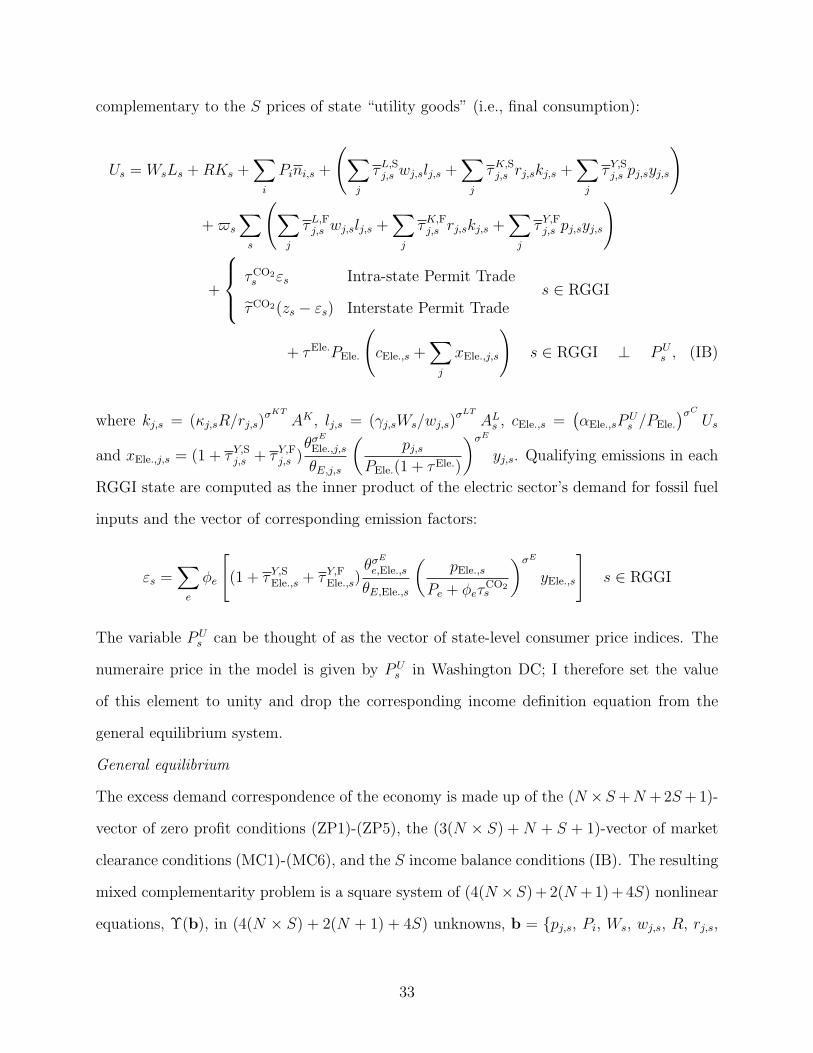
complementary to the S prices of state “utility goods” (i.e., final consumption):

Us = WsLs +RKs +∑

i

Pini,s +

(∑j

τL,Sj,s wj,slj,s +

∑j

τK,Sj,s rj,skj,s +

∑j

τY,Sj,s pj,syj,s

)

+$s

∑s

(∑j

τL,Fj,s wj,slj,s +

∑j

τK,Fj,s rj,skj,s +

∑j

τY,Fj,s pj,syj,s

)

+

τCO2s εs Intra-state Permit Trade

τCO2(zs − εs) Interstate Permit Trades ∈ RGGI

+ τEle.PEle.

(cEle.,s +

∑j

xEle.,j,s

)s ∈ RGGI ⊥ PU

s , (IB)

where kj,s = (κj,sR/rj,s)σKT

AK , lj,s = (γj,sWs/wj,s)σLT

ALs , cEle.,s =

(αEle.,sP

Us /PEle.

)σC

Us

and xEle.,j,s = (1 + τY,Sj,s + τY,F

j,s )θσE

Ele.,j,s

θE,j,s

(pj,s

PEle.(1 + τEle.)

)σE

yj,s. Qualifying emissions in each

RGGI state are computed as the inner product of the electric sector’s demand for fossil fuel

inputs and the vector of corresponding emission factors:

εs =∑

e

φe

[(1 + τY,S

Ele.,s + τY,FEle.,s)

θσE

e,Ele.,s

θE,Ele.,s

(pEle.,s

Pe + φeτCO2s

)σE

yEle.,s

]s ∈ RGGI

The variable PUs can be thought of as the vector of state-level consumer price indices. The

numeraire price in the model is given by PUs in Washington DC; I therefore set the value

of this element to unity and drop the corresponding income definition equation from the

general equilibrium system.

General equilibrium

The excess demand correspondence of the economy is made up of the (N ×S+N +2S+1)-

vector of zero profit conditions (ZP1)-(ZP5), the (3(N × S) +N + S + 1)-vector of market

clearance conditions (MC1)-(MC6), and the S income balance conditions (IB). The resulting

mixed complementarity problem is a square system of (4(N ×S)+2(N +1)+4S) nonlinear

equations, Υ(b), in (4(N × S) + 2(N + 1) + 4S) unknowns, b = pj,s, Pi, Ws, wj,s, R, rj,s,

33

PUs , yj,s, Yi, A

Ls , AK , Us.

34

Figure 1: The Representation of Production and Imperfect Factor Mobility in the Model

yj,s

σY = 0

Intermediate Materials

Energy Value-Added

σM = 0

xm,j,s

σE = 0.7

xe,j,s

σVA = 1 kj,s lj,s σM = Elasticity of substitution among intermediate material inputs (xm,j,s); σE = Elasticity of

substitution among intermediate energy inputs (xe,j,s); σV A = Elasticity of substitution betweenlabor (lj,s) and capital (kj,s); σY = Elasticity of substitution among energy, materials and

value-added.

(a) Industries’ nested production functions

σLT = 0.5

lj,d

σKT = 0.25

kj,d AKL

dA

σLA = 0.5

Lo

σKA = ∞

Ko

ALd = aggregate labor supply in destination state d; σLA = Elasticity of substitution among laborendowments of origin states o (Ko); σLT = Elasticity of transformation between aggregate andsector-specific labor at d (lj,d); AK = aggregate capital supply; σKA = Elasticity of substitution

among origin states’ capital endowments (Ko); σKT = Elasticity of transformation betweenaggregate and sector-specific capital (kj,d).

(b) Imperfect interstate and intersectoral factor mobility

35

Fig

ure

2:B

ench

mar

kYea

r-20

04In

terr

egio

nal

Soci

alA

ccou

nts

(Billion

$)

RG

GI

Par

tici

pati

ngSt

ates

Sout

hA

BC

Fin

.U

seTot

alA

BC

Fin

.U

seTot

alA

0.04

0.13

27.6

328

.52

56.3

2A

0.07

2.37

48.8

042

.27

93.5

1B

8.73

21.5

076

.01

-77.

7228

.52

B33

.09

173.

5287

.70

59.4

335

3.74

C9.

425.

1214

43.5

223

84.0

638

42.1

1C

18.0

972

.92

2640

.00

3533

.50

6264

.50

L6.

702.

4012

70.2

912

79.3

9L

11.2

417

.42

1845

.32

1873

.98

K16

.17

4.90

565.

4758

6.54

K34

.40

69.2

512

64.5

013

68.1

5T

10.3

32.

2340

3.77

416.

33T

14.9

314

.13

559.

2458

8.30

Tot

al51

.40

36.2

737

86.6

923

34.8

662

09.2

0Tot

al11

1.83

349.

5964

45.5

636

35.2

010

542.

18

Mid

wes

t(i

ncl.

PA)

Wes

tA

BC

Fin

.U

seTot

alA

BC

Fin

.U

seTot

alA

0.06

0.54

41.1

436

.10

77.8

3A

0.04

0.85

29.9

432

.23

63.0

6B

12.3

062

.66

69.2

1-2

3.70

120.

47B

11.9

156

.76

38.4

68.

5311

5.67

C14

.12

16.9

823

48.5

130

17.8

353

97.4

3C

9.23

26.2

816

39.1

626

93.9

243

68.5

9L

10.3

26.

8916

45.3

016

62.5

1L

7.16

8.23

1448

.83

1464

.22

K23

.86

14.3

892

9.00

967.

24K

14.7

525

.65

551.

1459

1.54

T13

.59

4.66

495.

3951

3.64

T10

.16

8.66

404.

3042

3.12

Tot

al74

.25

106.

1055

28.5

530

30.2

287

39.1

2Tot

al53

.25

126.

4341

11.8

327

34.6

870

26.1

9

A:

Ele

ctri

cPow

er;

B:

Foss

ilE

nerg

ySe

ctor

s;C

:N

on-E

nerg

ySe

ctor

s;L:

Lab

or;

K:

Cap

ital

;T

:co

mbi

ned

reve

nues

from

stat

ean

dfe

dera

lta

xes

onla

bor,

capi

talan

dpr

oduc

tion

.

36

Figure 3: Average Annual Growth Rates of State GDP and Energy Intensity, 2005-2015

-4%

-2%

0%

2%

4%

6%

8%

Ala

ska

Min

neso

taM

aine

Wes

t Virg

inia

Loui

sian

aO

klah

oma

Mis

sour

iM

onta

naIn

dian

aR

hode

Isla

ndM

aryl

and

Idah

oIo

wa

Con

nect

icut

Nev

ada

Wis

cons

inN

ew M

exic

oS

outh

Dak

ota

Kan

sas

Ken

tuck

yA

rkan

sas

Wyo

min

gA

laba

ma

Texa

sS

outh

Car

olin

aO

rego

nO

hio

Mis

siss

ippi

Neb

rask

aH

awai

iD

elaw

are

Flor

ida

Mic

higa

nN

orth

Car

olin

aD

ist.

of C

olum

bia

Nor

th D

akot

aM

assa

chus

etts

New

Jer

sey

New

Yor

kV

erm

ont

Uta

hV

irgin

iaTe

nnes

see

Was

hing

ton

Col

orad

oC

alifo

rnia

Pen

nsyl

vani

aG

eorg

iaN

ew H

amps

hire

Illin

ois

Ariz

ona

Pro

ject

ed A

vg. A

nnua

l Gro

wth

Rat

e

GDP GDP +/- 1 S.D. E/Y E/Y +/- 2 S.D. RGGI Participating States

37

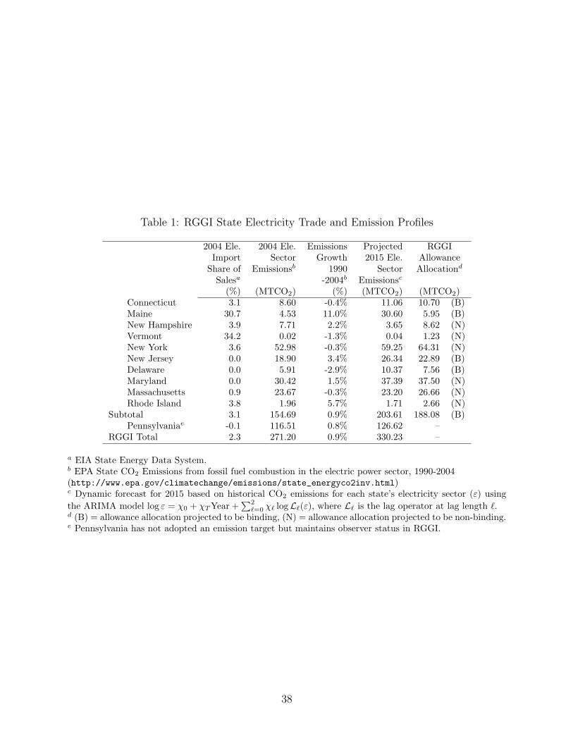
Table 1: RGGI State Electricity Trade and Emission Profiles

2004 Ele. 2004 Ele. Emissions Projected RGGIImport Sector Growth 2015 Ele. Allowance

Share of Emissionsb 1990 Sector Allocationd

Salesa -2004b Emissionsc

(%) (MTCO2) (%) (MTCO2) (MTCO2)Connecticut 3.1 8.60 -0.4% 11.06 10.70 (B)Maine 30.7 4.53 11.0% 30.60 5.95 (B)New Hampshire 3.9 7.71 2.2% 3.65 8.62 (N)Vermont 34.2 0.02 -1.3% 0.04 1.23 (N)New York 3.6 52.98 -0.3% 59.25 64.31 (N)New Jersey 0.0 18.90 3.4% 26.34 22.89 (B)Delaware 0.0 5.91 -2.9% 10.37 7.56 (B)Maryland 0.0 30.42 1.5% 37.39 37.50 (N)Massachusetts 0.9 23.67 -0.3% 23.20 26.66 (N)Rhode Island 3.8 1.96 5.7% 1.71 2.66 (N)

Subtotal 3.1 154.69 0.9% 203.61 188.08 (B)Pennsylvaniae -0.1 116.51 0.8% 126.62 –

RGGI Total 2.3 271.20 0.9% 330.23 –

a EIA State Energy Data System.b EPA State CO2 Emissions from fossil fuel combustion in the electric power sector, 1990-2004(http://www.epa.gov/climatechange/emissions/state_energyco2inv.html)c Dynamic forecast for 2015 based on historical CO2 emissions for each state’s electricity sector (ε) usingthe ARIMA model log ε = χ0 + χT Year +

∑2`=0 χ` logL`(ε), where L` is the lag operator at lag length `.

d (B) = allowance allocation projected to be binding, (N) = allowance allocation projected to be non-binding.e Pennsylvania has not adopted an emission target but maintains observer status in RGGI.

38

Tab

le2:

Res

ults

ofth

eA

nal

yti

calM

odel

(a)

Alg

ebra

icR

esul

ts

Ela

stic

ity

wit

hre

spec

tto

:ε A

τq A

1.C

arbo

n-en

ergy

ξ A−

(1−

β)/

∆(–

)[α

δ+

(1+

β)(

η+

σ(1−

α))

]/(α

∆)

(+)

pric

eξ N

−(1−

β)/

∆(–

)−

[αδ

+σ(1−

α)(

1−

β)]

/(α

∆)

(–)

2.E

lect

rici

tyq A

[2αδ

+(1

+β)(

η+

σ(1−

α))

]/∆

(+)

σ(1−

α)[

αδ

+(1

+β)(

η+

σ(1−

α))

]/(α

∆)

(+)

outp

utq N

−(1−

β)[

η+

σ(1−

α)]

/∆(–

)−

[η+

σ(1−

α)]

[αδ

+σ(1−

α)(

1−

β)]

/(α

∆)

(–)

3.E

lect

rici

typr

ice

π−

(1−

β)/

∆(–

)−

[αδ

+σ(1−

α)(

1−

β)]

/∆(–

)4.

Ele

ctri

city

t−

(1−

β)[

αδ

+(1

+β)(

η+

σ(1−

α))

]/(β

∆)

(–)

−[α

δ+

σ(1−

α)(

1−

β)]

(–)

trad

e×

[αδ

+(1

+β)(

η+

σ(1−

α))

]/(α

β∆

)5.

Car

bon-

ener

gyε N

−η(1−

β)/

∆(–

)−

η[α

δ+

σ(1−

α)(

1−

β)]

/(α

∆)

(–)

dem

and

E(1−

β)[

αδ

+σ(1−

α)]

/∆(+

)−

η(1−

β)[

αδ

+(1

+β)(

η+

σ(1−

α))

]/(2

α∆

)(–

)6.

Em

issi

onε A

−q A

σ(1−

α)(

1−

β)/

∆(+

)−

σ(1−

α)[

αδ

+(1

+β)(

η+

σ(1−

α))

]/(α

∆)

(–)

inte

nsity

ε N−

q Nσ(1−

α)(

1−

β)/

∆(+

)σ(1−

α)[

αδ

+σ(1−

α)(

1−

β)]

/(α

∆)

(+)

∆=

2αδ

+η(1

+β)+

2σ(1−

α)

>0

(b)

Num

eric

alR

esul

ts(α

=0.

3,β

=0.

03,δ

=0.

5,η

=1,

σ=

0.8)

RG

GI

RG

GI

Wit

hB

orde

rO

nly

Bor

der

Mea

sure

sM

easu

res

Onl

y(τ

q A=

0)(τ

q A=

τq A

,0)

(τq A

=τ

q A,0

)1.

Car

bon-

ener

gyξ A

0.03

00.

107

0.05

5pr

ice

ξ N0.

030

–-0

.052

2.E

lect

rici

tyq A

-0.0

59-0

.017

0.08

6ou

tput

q N0.

047

–-0

.081

3.E

lect

rici

typr

ice

π0.

009

–-0

.016

4.E

lect

rici

tytr

ade

t1.

768

–-3

.040

5.C

arbo

n-ε A

-0.0

76a

-0.0

76a

0.05

5en

ergy

ε N0.

030

–-0

.052

dem

and

E-0

.021

-0.0

37–

6.E

mis

sion

ε A−

q A-0

.017

-0.0

60-0

.031

inte

nsity

ε N−

q N-0

.017

–0.

029

7.Lea

kage

Λ0.

420

–1.

005

8.N

o-le

akag

eta

xτ

q A,0

0.03

20.

032a

0.03

2a

aE

xoge

nous

lyim

pose

dva

lues

.

39

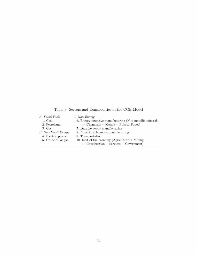
Table 3: Sectors and Commodities in the CGE Model

A. Fossil Fuels C. Non-Energy1. Coal 6. Energy-intensive manufacturing (Non-metallic minerals2. Petroleum + Chemicals + Metals + Pulp & Paper)3. Gas 7. Durable goods manufacturing

B. Non-Fossil Energy 8. Non-Durable goods manufacturing4. Electric power 9. Transportation5. Crude oil & gas 10. Rest of the economy (Agriculture + Mining

+ Construction + Services + Government)

40

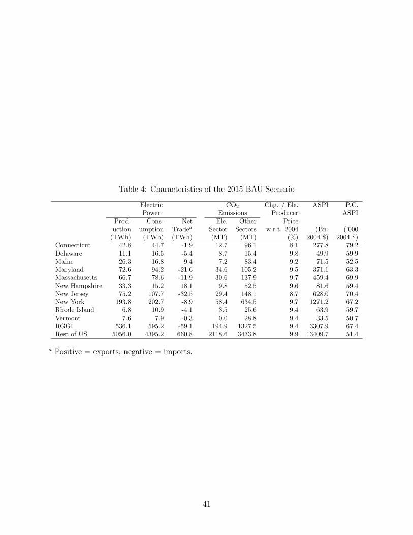
Table 4: Characteristics of the 2015 BAU Scenario

Electric CO2 Chg. / Ele. ASPI P.C.Power Emissions Producer ASPI

Prod- Cons- Net Ele. Other Priceuction umption Tradea Sector Sectors w.r.t. 2004 (Bn. (’000

(TWh) (TWh) (TWh) (MT) (MT) (%) 2004 $) 2004 $)Connecticut 42.8 44.7 -1.9 12.7 96.1 8.1 277.8 79.2Delaware 11.1 16.5 -5.4 8.7 15.4 9.8 49.9 59.9Maine 26.3 16.8 9.4 7.2 83.4 9.2 71.5 52.5Maryland 72.6 94.2 -21.6 34.6 105.2 9.5 371.1 63.3Massachusetts 66.7 78.6 -11.9 30.6 137.9 9.7 459.4 69.9New Hampshire 33.3 15.2 18.1 9.8 52.5 9.6 81.6 59.4New Jersey 75.2 107.7 -32.5 29.4 148.1 8.7 628.0 70.4New York 193.8 202.7 -8.9 58.4 634.5 9.7 1271.2 67.2Rhode Island 6.8 10.9 -4.1 3.5 25.6 9.4 63.9 59.7Vermont 7.6 7.9 -0.3 0.0 28.8 9.4 33.5 50.7RGGI 536.1 595.2 -59.1 194.9 1327.5 9.4 3307.9 67.4Rest of US 5056.0 4395.2 660.8 2118.6 3433.8 9.9 13409.7 51.4

a Positive = exports; negative = imports.

41

Table 5: Impacts of RGGI Emission Targets

Change in Electricity Chg. / CO2 Chg. / Ele. Chg. / Allow-Market w.r.t. BAU Emissions Producer P.C. ance

Prod- Cons- Net Ele. Other Price ASPI Priceuction umption Tradea Sector Sectors w.r.t. BAU

(%) (%) (%) (MT) (MT) (%) ($) ($)A. Intra-state Allowance Trading

Connecticut -2.9 -0.2 58.5 -2.0 0.1 1.3 20.9 24Delaware -3.0 -0.2 5.7 -1.1 0.0 1.3 57.1 12Maine -13.3 -0.1 -36.9 -1.2 0.0 4.2 164.5 55Maryland 0.2 -0.2 -1.8 0.1 0.1 0.5 -8.5 0Massachusetts -3.1 -0.2 16.2 -4.0 0.1 1.4 24.0 16New Hampshire -1.6 -0.2 -2.8 -1.2 0.0 1.0 49.5 13New Jersey -7.3 -0.1 16.5 -6.5 0.1 2.5 83.0 60New York 0.3 -0.3 -11.7 0.2 0.3 0.5 -7.3 0Rhode Island -24.8 0.0 41.7 -0.9 0.0 8.0 265.9 147Vermont 0.3 -0.3 -12.9 0.0 0.0 0.5 -3.3 0RGGI -2.7 -0.2 21.9 -16.6 0.8 1.2 28.6 –Rest of US 0.3 -0.2 3.8 8.3 2.7 0.5 -6.8 –

B. Interstate Allowance TradingConnecticut -0.3 0.0 7.1 -0.5 0.0 0.2 1.8 2.8Delaware -0.7 0.0 1.5 -0.4 0.0 0.3 13.1 2.8Maine -0.6 0.0 -1.6 -0.1 0.0 0.2 7.8 2.8Maryland -0.5 0.0 1.5 -1.1 0.0 0.2 12.0 2.8Massachusetts -0.6 0.0 3.0 -1.1 0.0 0.2 4.2 2.8New Hampshire -0.4 0.0 -0.7 -0.4 0.0 0.2 11.4 2.8New Jersey -0.3 0.0 0.7 -1.1 0.0 0.2 2.1 2.8New York -0.3 0.0 6.2 -2.1 0.0 0.2 4.4 2.8Rhode Island -0.3 0.0 0.5 0.0 0.0 0.2 3.5 2.8Vermont 0.0 0.0 -1.4 0.0 0.0 0.1 4.8 2.8RGGI -0.4 0.0 3.3 -6.8 0.1 0.2 5.1 2.8Rest of US 0.1 0.0 0.6 2.2 1.0 0.1 -1.1 –

C. Interstate Allowance Trading+ Harmonized Zero-Leakage (2.5%) Electricity Tariff

Connecticut -0.5 -1.1 -14.6 -0.5 0.2 -0.1 8.0 2.7Delaware -0.8 -1.0 -1.2 -0.4 0.1 0.0 22.4 2.7Maine -0.7 -1.2 0.1 -0.1 0.1 0.0 13.7 2.7Maryland -0.6 -0.9 -2.1 -1.1 0.3 0.0 20.5 2.7Massachusetts -0.7 -1.0 -3.0 -1.1 0.4 0.0 9.9 2.7New Hampshire -0.5 -1.1 0.0 -0.4 0.1 -0.1 21.0 2.7New Jersey -0.4 -1.0 -2.2 -1.1 0.5 -0.1 8.1 2.7New York -0.4 -1.1 -15.7 -2.1 1.4 -0.1 11.1 2.7Rhode Island -0.4 -1.1 -2.1 0.0 0.1 -0.1 9.1 2.7Vermont -0.1 -1.1 -26.1 0.0 0.0 -0.2 10.3 2.7RGGI -0.5 -1.0 -5.8 -6.8 3.3 -0.1 11.8 2.7Rest of US -0.1 0.1 -0.9 0.1 -3.5 -0.2 -2.5 –

a Positive = exports; negative = imports.

42

Table 6: Impact of RGGI on Components of ASPI (% Change)

Factor Income Net Recycled Revenue TotalLabor Capital Foreign Federal State Allow- Electricity

Assets Taxes Taxes ancesa Tariffsa

A. Intra-state Allowance TradingConnecticut -0.10 -0.03 0.16 -0.03 -0.07 1.04 – 0.03Delaware -0.11 -0.03 -0.45 -0.03 -0.09 1.84 – 0.09Maine -0.23 -0.03 0.15 -0.03 -0.35 9.07 – 0.31Maryland -0.01 -0.03 0.14 -0.03 0.02 0.00 – -0.01Massachusetts -0.08 -0.03 0.16 -0.03 -0.09 1.66 – 0.03New Hampshire -0.07 -0.03 0.14 -0.03 -0.05 1.53 – 0.08New Jersey -0.14 -0.03 0.18 -0.03 -0.20 3.65 – 0.12New York -0.01 -0.03 0.16 -0.03 0.02 0.00 – -0.01Rhode Island -0.24 -0.03 0.16 -0.03 -0.65 15.92 – 0.44Vermont -0.01 -0.03 0.15 -0.03 0.02 0.00 – -0.01RGGI Total -0.07 -0.03 0.16 -0.03 -0.06 1.32 – 0.04

B. Interstate Allowance TradingConnecticut -0.01 0.00 0.04 -0.01 -0.02 0.13 – 0.00Delaware -0.03 -0.01 -0.36 -0.01 -0.07 0.46 – 0.02Maine -0.01 0.00 0.03 -0.01 -0.10 0.52 – 0.01Maryland -0.01 0.00 0.02 -0.01 0.04 0.40 – 0.02Massachusetts -0.01 0.00 0.04 -0.01 -0.05 0.31 – 0.01New Hampshire -0.02 0.00 0.03 -0.01 -0.04 0.36 – 0.02New Jersey -0.01 -0.01 0.04 -0.01 -0.05 0.20 – 0.00New York -0.01 0.00 0.04 -0.01 0.02 0.16 – 0.01Rhode Island -0.01 0.00 0.04 -0.01 -0.10 0.38 – 0.01Vermont 0.00 0.00 0.03 -0.01 0.09 0.00 – 0.01RGGI Total -0.01 0.00 0.03 -0.01 -0.01 0.22 – 0.01

C. Interstate Allowance Trading+ Harmonized Zero-Leakage (2.5%) Electricity Tariff

Connecticut -0.06 -0.04 0.08 -0.04 -0.06 0.13 0.51 0.01Delaware -0.07 -0.04 -0.34 -0.04 -0.10 0.45 0.57 0.04Maine -0.06 -0.04 0.07 -0.04 -0.13 0.51 0.93 0.02Maryland -0.05 -0.04 0.06 -0.04 0.00 0.39 0.83 0.03Massachusetts -0.06 -0.04 0.07 -0.04 -0.08 0.30 0.83 0.01New Hampshire -0.06 -0.04 0.06 -0.04 -0.08 0.35 0.63 0.03New Jersey -0.05 -0.04 0.09 -0.04 -0.08 0.20 0.78 0.01New York -0.06 -0.04 0.07 -0.04 -0.02 0.16 0.66 0.02Rhode Island -0.05 -0.04 0.07 -0.04 -0.13 0.37 1.19 0.01Vermont -0.05 -0.04 0.07 -0.04 0.05 0.00 0.45 0.02RGGI Total -0.06 -0.04 0.07 -0.04 -0.04 0.22 0.71 0.02

a Value of allowances expressed as a fraction of recycled revenue from pre-existing state taxes.b Revenue generated by countervailing tariff on electric power in each state, recycled to the correspondingrepresentative agent.

43

Tab

le7:

Res

ults

ofSen

siti

vity

Anal

ysi

s:R

GG

IW

ithou

tB

order

Mea

sure

s

Chg.

/C

hg.

/E

le.

Chg.

/C

hange

inLea

kage

Allow

-C

hg.

/E

le.

CO

2In

tensi

tyA

rm-

CO

2E

mis

sions

ance

P.C

.N

etR

GG

IR

est

ingto

nU

.S.

RG

GI

RG

GI

Inte

rnal

Exte

rnal

Exte

rnal

U.S

.Λ

Pri

ceA

SP

ITra

dea

ofU

.S.

Ele

.N

etE

le.

Tota

lE

le.

Non-E

le.

Net

Pri

ceSec

tor

Sec

tor

Sec

tor

(%)

(%)

(%)

(%)

(MT

)(M

T)

(MT

)(M

T)

(MT

)(M

T)

(MT

)(%

)($

/to

n)

($)

A.B

ase

Case

3.3

-3.1

0.0

50.0

8-3

.4-6

.8-6

.70.1

2.2

1.0

3.4

49

2.8

5.1

B.E

ner

gy

Inte

nsi

tyΩ

=-0

.51

(+2

S.D

.)7.6

-5.5

0.1

00.1

9-6

.1-1

2.8

-12.6

0.2

4.6

1.9

6.7

53

6.2

11.2

Ω=

-0.7

1(-

2S.D

.)0.4

-0.5

0.0

10.0

1-0

.5-1

.0-1

.00.0

0.3

0.2

0.5

47

0.3

0.6

1%

p.a

.A

EE

I20.1

-9.0

0.1

70.4

9-9

.4-2

3.2

-22.7

0.6

10.0

3.2

13.9

60

15.3

26.6

0.5

%p.a

.A

EE

I42.2

-11.4

0.2

21.0

0-1

0.5

-34.4

-33.2

1.2

18.1

4.6

24.0

70

29.8

50.7

C.A

vg.

GSP

Gro

wth

Rate

s+

1S.D

.10.6

-8.8

0.1

50.2

9-1

0.3

-20.8

-20.5

0.4

6.9

3.3

10.6

51

10.1

17.6

-1S.D

.0.0

0.0

0.0

00.0

00.0

0.0

0.0

0.0

0.0

0.0

0.0

0.0

0.0

D.In

terf

uel

Ela

stic

itie

sofSubst

itution

σE

=1.4

(2×

)2.0

-3.6

0.0

90.0

4-3

.2-7

.5-7

.40.1

2.7

1.5

4.3

57

1.6

3.0

σE

=0.3

5(0

.5×

)6.0

-2.7

0.0

30.1

7-3

.3-6

.6-6

.50.1

2.5

0.7

3.3

50

5.3

9.4

E.A

rmin

gto

nE

last

icitie

sofSubst

itution

σA Ele

c.=

8(2×

)3.4

-3.0

0.0

50.0

8-3

.3-6

.6-6

.50.1

2.2

1.0

3.3

50

2.7

4.6

σA Ele

c.=

2(0

.5×

)3.3

-3.3

0.0

60.0

9-3

.7-7

.1-7

.00.1

2.2

1.1

3.4

48

3.0

6.0

2×

σA e6=

Ele

c.

3.4

-3.1

0.0

50.0

8-3

.5-6

.9-6

.80.1

2.2

1.1

3.4

49

2.8

5.1

0.5×

σA e6=

Ele

c.

3.3

-3.1

0.0

50.0

8-3

.4-6

.7-6

.60.1

2.2

1.0

3.3

49

2.8

5.1

aPos

itiv

e=

expo

rts;

nega

tive

=im

port

s.

44

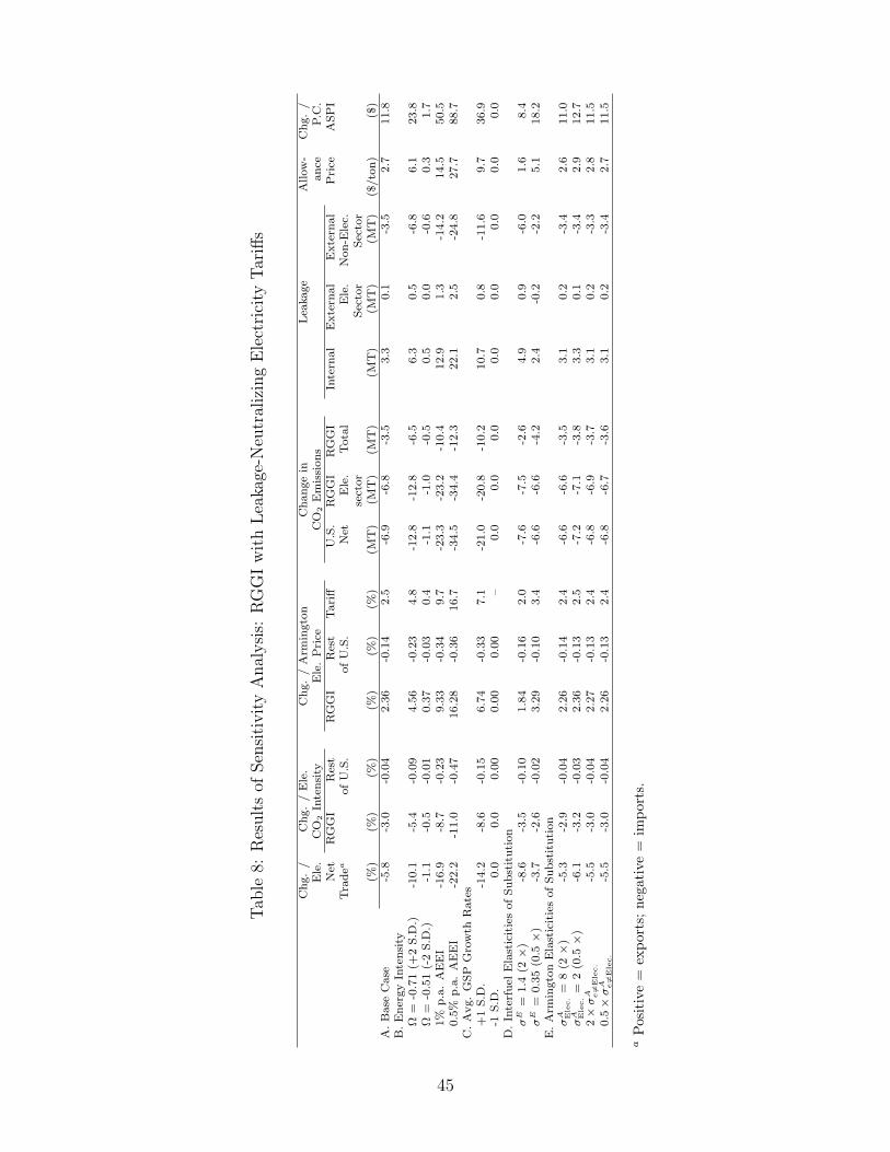
Tab

le8:

Res

ult

sof

Sen

siti

vity

Anal

ysi

s:R

GG

Iw

ith

Lea

kage

-Neu

tral

izin

gE

lect

rici

tyTar

iffs

Chg.

/C

hg.

/E

le.

Chg.

/A

rmin

gto

nC

hange

inLea

kage

Allow

-C

hg.

/E

le.

CO

2In

tensi

tyE

le.

Pri

ceC

O2

Em

issi

ons

ance

P.C

.N

etR

GG

IR

est

RG

GI

Res

tTari

ffU

.S.

RG

GI

RG

GI

Inte

rnal

Exte

rnal

Exte

rnal

Pri

ceA

SP

ITra

dea

ofU

.S.

ofU

.S.

Net

Ele

.Tota

lE

le.

Non-E

lec.

sect

or

Sec

tor

Sec

tor

(%)

(%)

(%)

(%)

(%)

(%)

(MT

)(M

T)

(MT

)(M

T)

(MT

)(M

T)

($/to

n)

($)

A.B

ase

Case

-5.8

-3.0

-0.0

42.3

6-0

.14

2.5

-6.9

-6.8

-3.5

3.3

0.1

-3.5

2.7

11.8

B.E

ner

gy

Inte

nsi

tyΩ

=-0

.71

(+2

S.D

.)-1

0.1

-5.4

-0.0

94.5

6-0

.23

4.8

-12.8

-12.8

-6.5

6.3

0.5

-6.8

6.1

23.8

Ω=

-0.5

1(-

2S.D

.)-1

.1-0

.5-0

.01

0.3

7-0

.03

0.4

-1.1

-1.0

-0.5

0.5

0.0

-0.6

0.3

1.7

1%

p.a

.A

EE

I-1

6.9

-8.7

-0.2

39.3

3-0

.34

9.7

-23.3

-23.2

-10.4

12.9

1.3

-14.2

14.5

50.5

0.5

%p.a

.A

EE

I-2

2.2

-11.0

-0.4

716.2

8-0

.36

16.7

-34.5

-34.4

-12.3

22.1

2.5

-24.8

27.7

88.7

C.A

vg.

GSP

Gro

wth

Rate

s+

1S.D

.-1

4.2

-8.6

-0.1

56.7

4-0

.33

7.1

-21.0

-20.8

-10.2

10.7

0.8

-11.6

9.7

36.9

-1S.D

.0.0

0.0

0.0

00.0

00.0

0–

0.0

0.0

0.0

0.0

0.0

0.0

0.0

0.0

D.In

terf

uel

Ela

stic

itie

sofSubst

itution

σE

=1.4

(2×

)-8

.6-3

.5-0

.10

1.8

4-0

.16

2.0

-7.6

-7.5

-2.6

4.9

0.9

-6.0

1.6

8.4

σE

=0.3

5(0

.5×

)-3

.7-2

.6-0

.02

3.2

9-0

.10

3.4

-6.6

-6.6

-4.2

2.4

-0.2

-2.2

5.1

18.2

E.A

rmin

gto

nE

last

icitie

sofSubst

itution

σA Ele

c.=

8(2×

)-5

.3-2

.9-0

.04

2.2

6-0

.14

2.4

-6.6

-6.6

-3.5

3.1

0.2

-3.4

2.6

11.0

σA Ele

c.=

2(0

.5×

)-6

.1-3

.2-0

.03

2.3

6-0

.13

2.5

-7.2

-7.1

-3.8

3.3

0.1

-3.4

2.9

12.7

2×

σA e6=

Ele

c.

-5.5

-3.0

-0.0

42.2

7-0

.13

2.4

-6.8

-6.9

-3.7

3.1

0.2

-3.3

2.8

11.5

0.5×

σA e6=

Ele

c.

-5.5

-3.0

-0.0

42.2

6-0

.13

2.4

-6.8

-6.7

-3.6

3.1

0.2

-3.4

2.7

11.5

aPos

itiv

e=

expo

rts;

nega

tive

=im

port

s.

45

References

Arellano, M. and S. Bond (1991). Some tests of specification for panel data: Monte Carlo

evidence and an application to employment equations. Review of Economic Studies 58,

277–197.

Armington, P. S. (1969). A theory of demand for products distinguished by place of produc-

tion. IMF Staff Papers 16, 159–176.

Babiker, M. H. (2001). Subglobal climate-change actions and carbon leakage: The implica-

tion of international capital flows. Energy Economics 23, 121–139.

Babiker, M. H. (2005). Climate change policy, market structure, and carbon leakage. Journal

of International Economics 65, 421–445.

Babiker, M. H. and T. F. Rutherford (2005). The economic effects of border measures in

subglobal climate agreements. Energy Journal 26, 101–128.

Bolster, H. D. (2006). The commerce clause meets environmental protection: The compen-

satory tax doctrine as a defense of potential regional carbon dioxide regulation. Boston

College Law Review 47, 772–737.

Burtraw, D., D. Kahn, and K. Palmer (2006). CO2 allowance allocation in the Regional

Greenhouse Gas Initiative and the effect on electricity investors. Electricity Journal 19,

79–90.

Copeland, B. R. and M. S. Taylor (2005). Free trade and global warming: a trade theory

view of the Kyoto Protocol. Journal of Environmental Economics and Management 49,

205–234.

Farnsworth, D., C. Palmero, and C. Sherry (2007). Potential emissions leakage and the

Regional Greenhouse Gas Initiative (RGGI): Evaluating market dynamics, monitoring op-

46

tions, and possible mitigation mechanisms—initial report of the RGGI Emissions Leakage

Multi-State Staff Working Group. Technical report, Regional Greenhouse Gas Initiative.

Felder, S. and T. F. Rutherford (1993). Unilateral CO2 reductions and carbon leakage: The

consequences of international trade in oil and basic materials. Journal of Environmental

Economics and Management 25, 162–176.

Fullerton, D. and G. E. Metcalf (2002). Tax incidence. In A. Auerbach and M. Feldstein

(Eds.), Handbook of Public Economics, vol. 4, pp. 1787–1872. Elsevier.

Gerlagh, R. and O. Kuik (2007). Carbon leakage with international technology spillovers.

Working Paper No. 2007-48, Fondazione Eni Enrico Mattei.

Jacoby, H. D. and A. D. Ellerman (2004). The safety valve and climate policy. Energy

Policy 32, 481–491.

Metcalf, G. E. (2007). An empirical analysis of energy intensity and its determinants at the

state level. Energy Journal forthcoming.

Nuclear Energy Agency/International Energy Agency (2005). Projected Costs of Generating

Electricity: 2005 Update. Paris: OECD.

Stavins, R. N. (2006). A utility safety valve for cutting CO2. The Environmental Forum 23,

14.

Sue Wing, I. (2005). The synthesis of bottom-up and top-down approaches to climate policy

modeling: Electric power technologies and the cost of limiting U.S. CO2 emissions. Energy

Policy 34, 3847–3869.

Sue Wing, I. (2007). The regional impacts of U.S. climate change policy: A general equilib-

rium analysis. mimeo, Boston University.

Sue Wing, I. and R. S. Eckaus (2007). The decline in U.S. energy intensity: Its origins and

implications for long-run co2 emission projections. Energy Policy 35, 5267–5286.

47

Weiner, J. B. (2007). Think globally, act globally: The limits of local climate policies.

University of Pennsylvania Law Review 155, 1961–1979.

48