Regional economic impacts of greenhouse gas emission mitigation policies in brazilian

agriculture: the role of the degraded paste recovery program

Géssica C. P. Souza1

Edson Paulo Domingues2

Aline Magalhães3

ABSTRACT

This paper estimates the regional economic impacts of a Brazilian public policy aimed at mitigating

greenhouse gases on agriculture. More specifically the Degraded Pasture Recovery Program (RPD)

of the ABC Plan during the period from 2015 to 2018 and the projected period (2019 to 2025). A

computable general equilibrium (EGC) model is constructed and regionalized especially for this

simulation, in order to differentiate geographical spaces according to their geomorphological, climatic

and pedological characteristics. Results indicate different impacts between regions and sectors. The

greater the representativeness of the ABC plan financing in relation to the value of production in the

livestock sectors, the greater the accumulated decrease of the region's GDP. The policy is essential for

the economic growth of regions that do not necessarily have large livestock production but have a high

ratio between production and value financed by the program. In addition, the impact on production

goes beyond the livestock sectors and may interfere with the production of a range of sectors that are

important to the economy, both agriculturally and industrially.

Keywords: mitigation policy; environmental; degraded pasture; computable general equilibrium

model

1 INTRODUCTION

Climate change, mainly caused by anthropic interference, has been shown to be one of

humanity's greatest current challenges (MCTI, 2015). The entire planet earth is vulnerable to climate

change and may present significant socioeconomic and environmental problems. Thus, a schedule

global aimed at minimizing global environmental problems was consolidated in 1992 along with the

elaboration of the United Nations Framework Convention on Climate Change (UNFCCC). Aiming at

economic and social growth combined with environmental preservation and climate balance, countries

have been implementing policies to significantly reduce emissions and increase sinks of greenhouse

gases.

Brazil, at the 15th Conference of the Parties - COP15, in 2009, pledged to reduce greenhouse

gas (GHG) emissions by 36.1% to 38.9% by 2020. Among the policies implemented by Brazil aimed

at Fulfilling its international commitments is the Sectoral Climate Change Mitigation and Adaptation

Plan for the Consolidation of a Low Carbon Economy in Agriculture - Plan ABC.

1 Federal Univeristy of Minas Gerias. Email: gessicacardoso@cedeplar.ufmg.br 2 Federal Univeristy of Minas Gerias. Email: epdomin@cedeplar.ufmg.br 3 Federal Univeristy of Minas Gerias. Email: alinesm@cedeplar.ufmg.br

Agriculture and livestock activities, as well as the land use and forestry change sector are the

main GHG emitters in Brazil. Together they account for a quarter of gross national emissions

(considering all emission sources) (MCTI, 2015). In addition to contributing significantly to carbon

emissions in the atmosphere, the agricultural sector is also extremely climate sensitive, making

production vulnerable to likely climate change. As Brazil is among the world's largest producers and

exporters of agricultural products, stimulating industry growth and reducing greenhouse gas emissions

are two challenges to be overcome.

Thus, according to the Ministry of Agriculture, Livestock and Supply - MAPA (2012), the

ABC Plan is a sectoral public policy whose general objective is to promote the reduction of GHG

emissions in agriculture, improving the efficiency of the use of natural resources and increasing the

resilience of production systems and rural communities, enabling the adaptation of the agricultural

sector to climate change, ensuring productivity.

The ABC Plan, approved in 2011, is nationwide with a period of validity up to 2020. The Plan's

goal is to reduce GHG emissions in agriculture by 134 to 163 million tons of CO2 through seven

programs, six of them referring to mitigation technologies and the last one with actions to adapt to

climate change. One of the mitigation programs, called Degraded Pasture Recovery (RPD), aims to

recover 15 million of the country's current 63 million hectares of degraded pasture (LAPIG, 2017).

For the execution of the ABC Plan, the then Program for the Reduction of Greenhouse Gas

Emissions in Agriculture (ABC Program) was prepared, a credit program associated with Rural Credit,

with subsidized interest rates. The amount of funds made available, the credit limits to the producer,

the maximum repayment period, the grace period and the interest rates are adjusted annually. For the

2018/2019 crop year, there was an increase in the credit limit for all purposes financed by the Program,

as well as an interest rate drop from 7.5% to 6% to 5.25%, depending on the purpose of the financing

( MAP, 2012).

Initially, an estimated amount of R $ 152.3 billion (OBSERVATORIO ABC, 2017b) was

required to implement the ABC Plan objectives from 2010 to 2020. However, according to data

released by the Central Bank, the amounts financed by the Plan in january 2013 to December 2019 are

equivalent to only R $ 14.4 billion, or 9.5% of the initial estimate. The reports released by the ABC

Observatory (2013, 2014) cite, mainly, bureaucratic difficulties on the part of farmers to obtain credit.

The ABC Plan requires a technical project attesting the potential for GHG productivity and mitigation

against other less bureaucratic and fast rural credit lines.

Historically, among all programs, RPD has the highest demand for funding, which is justified

by its ease of implementation, unlike, for example, the more complex implementation of Crop-

Livestock-Forest (iLPF) program. , resulting in lower adherence by small and medium farmers.

Between 2016 and 2019 (focus period of this research) the RPD program received R $ 3.1 billion of

funding, which is equivalent to 49% of the total funded by the ABC Plan during this period. The

Brazilian states that most received funding for RPD were Goiás, Minas Gerais and Tocantins, totaling

R $ 1.3 billion, which is equivalent to 43% of the national total.

Regarding the goals achieved by the ABC Plan over the ten years of implementation, the ABC

Platform Periodic Estimates Technical Note (MAPA, 2018)) produced estimates of expansion of

adoption (in hectares) and mitigation (million Mg CO2 eq) of the Plan. According to the report,

mitigation technologies were adopted over a total area of 27.65 Mha, corresponding to 77% of the

target set and mitigating a total of 100.21 million Mg CO2 eq., 68% of the target. Regarding the RPD

program, 4.46 Mha of pastures were recovered by 2018, corresponding to 30% of the target range.

Thus, there was a mitigation of 16.9 million Mg CO2 eq, reaching 18% of the established target.

As the ABC Plan expires in 2020, policy revisions and updates are planned, adjusting it to

societal demands, new technologies and incorporating new actions and goals. The new Brazilian

challenge set in Paris during the 2015 United Nations Conference on Climate Change (COP 21) is to

reduce greenhouse gas emissions by 37% by 2025 and 43% by 2030, compared to 2005 levels. Thus,

the challenge is to expand the area of iLPF and RDP by 20 Mha by 2030.

Therefore, understanding the economic and not only environmental impacts achieved during

the last years and projecting the possible compensations for a policy renewal is extremely important.

Thus, the main objective of this research is to estimate the regional economic impacts of the degraded

pasture recovery (RPD) program of the ABC Plan during the period from 2015 to 2018 and the

projected period (2019 to 2025). As this is a financing policy that has already been implemented and

is in its final stage, a fall in livestock activity will be simulated in proportion to the amount financed

by the program from 2015 to 2018. Thus, the impacts resulting from the absence of the policy will

allow an assessment of its regional, sectoral and macroeconomic importance.

This article is further subdivided into 4 sections in addition to this introduction. The second

section presents a brief literature review that analyzes the economic impacts of climate change and

mitigation policies. Section 3 then details the computable general equilibrium model developed for the

analysis in question. Following, section 4 details the scenarios and closure adopted. In section 5 the

results found are reported and discussed. And the final section weaves the main conclusions of the

study.

2 ECONOMIC IMPACTS OF CLIMATE CHANGE AND MITIGATION POLICIES

According to Fischer et al. (2002), climate change may impact not only environmental but also

social and economic systems. Using ecological-economic integration models, these authors assessed

the agroecological impact of climate change and concluded that developing regions will suffer a loss

in grain yield in all scenarios analyzed. The overall decrease in cereal production may range from –

0.7% to –1.2% in 2080. And African countries' GDP may fall by 7 to 9%, although overall GDP may

grow to 2, 6% in the period analyzed.

For Brazil, Domingues et al. (2008) analyze the impacts of climate change in the Northeast.

The authors use an interregional Computable General Equilibrium (EGC) model that considers the

availability of unsuitable land for agricultural activity according to Embrapa estimates (2008) and

considers the global warming scenarios of the International Panel of Climate. Change (IPCC). The

results indicate a loss of -13.1% of GDP and -5.95% of employment in the region in 2050, compared

to the reference scenario, with Pernambuco, Piauí, Paraíba and Ceará being the most affected Brazilian

states. The agricultural activity presents a fall of 70.6% and the economic effects on employment, can

generate significant impacts on migratory flows.

Moraes (2010) also uses an EGC model to measure the effects of climate change on Brazilian

agricultural production. Similarly to Domingues et al. (2008), land was considered a factor of

agricultural production according to the suitability of Embrapa (2008). According to the results, in the

scenario of less severe and more severe climate change, the Northeast and the Midwest are the regions

most affected. There is a drop in overall economic activity of 0.29% of GDP in 2020 and 1.09% in

2070 and a drop in agricultural activities at the national level, most significantly in soybean and coffee

production.

Using a dynamic, recursive and interregional ECG model, Ferreira Filho and Horridge (2010)

analyze the potential impacts of climate change scenarios on Brazilian agriculture on internal

migrations in Brazil. The authors find modest results of cumulative GDP variation and real investment,

falling by -0.82% and -0.5% respectively by 2070. Soybean and coffee production would be the most

affected by climate change and unlike other studies, the Northeast region would not be the most

affected but the state of Mato Grosso do Sul, with a reduction in GDP of -4.13%.

The study Economics of Climate Change in Brazil (MARGULIS AND DUBEUX, 2010) also

sought to measure the impacts of climate change on the Brazilian economy by integrating different

models, including the EFES general equilibrium model. The results indicate a cumulative GDP loss of

-0.5%, considering IPCC scenario A2, and -2.3% in scenario B2, from 2008 to 2050. In both scenarios,

poverty increases, but of almost negligible way and the reductions in consumption of Brazilians,

accumulated until 2050, would represent a fall of 60% to 180% of the per capita annual consumption

of 2010.

Several types of mitigation policies have been adopted by countries, but little is known about

the possible economic and social impacts of such mechanisms. As noted by Magalhães and Domingues

(2013), aggressive GHG emission reduction policies may be an obstacle to growth or may be regressive

from a distributive point of view. In this sense, using a dynamic-recursive general equilibrium model,

the authors analyze alternative policies to reduce price-induced emissions, such as carbon taxation.

Regarding the share of emissions related to fuel use, the authors conclude that ambitious emission

reduction targets must be associated with long periods of time, as the Brazilian energy matrix is

intensive in “clean” sources. Otherwise, a very high cost would be imposed on the Brazilian economy.

Regarding the effects on income classes, the results indicated that carbon taxation has a regressive

effect both in terms of consumption and changes in the Gini coefficient.

The study Economics of Climate Change in Brazil (MARGULIS AND DUBEUX, 2010) also

sought to measure the impacts of climate change on the Brazilian economy by integrating different

models, including the EFES general equilibrium model. The results indicate a cumulative GDP loss of

-0.5%, considering IPCC scenario A2, and -2.3% in scenario B2, from 2008 to 2050. In both scenarios,

poverty increases, but of almost negligible way and the reductions in consumption of Brazilians,

accumulated until 2050, would represent a fall of 60% to 180% of the per capita annual consumption

of 2010.

Several types of mitigation policies have been adopted by countries, but little is known about

the possible economic and social impacts of such mechanisms. As noted by Magalhães and Domingues

(2013), aggressive GHG emission reduction policies may be an obstacle to growth or may be regressive

from a distributive point of view. In this sense, using a dynamic-recursive general equilibrium model,

the authors analyze alternative policies to reduce price-induced emissions, such as carbon taxation.

Regarding the share of emissions related to fuel use, the authors conclude that ambitious emission

reduction targets must be associated with long periods of time, as the Brazilian energy matrix is

intensive in “clean” sources. Otherwise, a very high cost would be imposed on the Brazilian economy.

Regarding the effects on income classes, the results indicated that carbon taxation has a regressive

effect both in terms of consumption and changes in the Gini coefficient.

Gurgel (2012), using the Emissions Prediction and Policy Analysis (EPPA) model (PALTSEV

et al., 2005), seeks to evaluate how the adoption of new low carbon technologies and the introduction

of restrictions on GHG emissions can change the structure. relative prices and the competitiveness of

Brazilian products and sectors. The results indicate that mitigation via deforestation reduction in Brazil

produces a slight decrease of -0.3% of GDP, however, intensification of the policy can generate losses

that reach -4% of GDP in 2050. In addition, the author concludes that adopting global climate policies

would reduce mitigation costs in developed countries through carbon trading, as well as achieving a

steady and satisfactory level of emissions.

Carvalho (2014) seeks to analyze the economic losses resulting from deforestation control

policies in the Legal Amazon through the REGIA model, of the interregional and dynamic type.

Among the simulations a control policy aimed at reducing deforestation by 80% by 2020, followed by

a 100% reduction target for the period between 2021 and 2030 indicated a cumulative fall in Legal

Amazon GDP of -1.06%, in relation to the reference scenario. The Brazilian states that would lose the

most with the control of deforestation would be: Mato Grosso (-1.88%), Rondônia (-1.55%), Acre (-

1.35%) and Pará (-0.95%). Employment also declines, as do household income and consumption,

indicating that the policy causes a loss of well-being.

Regarding the ABC Plan, there are few studies that evaluate the economic impacts of the policy.

There are studies in the literature of the ABC Observatory (2017b) and Lima (2017). Both sought to

quantify the economic and environmental impacts of the policy, but specifically the Degraded Pasture

Recovery (RPD) and Crop-Livestock-Forest Integration (iLPF) programs. They use an EGC model

calibrated for 2009, representing the five Brazilian macroregions plus the MATOPIBA region

(Maranhão, Tocantins, Piauí and Bahia states). Two scenarios are analyzed, in the first the RPD is

implemented in the most degraded pastures and in the second, the recovery is made by free allocation.

This second scenario simulates how the program actually occurs, since there is no pre-definition of

priority areas for the program.

The results show that investment expenditures to meet the plan's targets are lower than

originally planned and that the ABC Program's level of resource adoption is well below the amount

that would be required to meet the mitigation targets. There is also a “land-saving effect” with the

implementation of the programs, allowing an increase of at least 4.8 Mha in forest and secondary

vegetation areas.

Regarding welfare, the results indicate a loss and R $ 3.71 of consumption per inhabitant in the

first scenario and a gain of R $ 41.18 in the second. Regarding environmental impacts, the potential

accumulation in the carbon stock of forest formations and natural vegetation would be greater if pasture

recovery occurred in the priority areas. In addition, if the RPD and iLPF targets were achieved,

between 32% and 39% of the total emission reduction target for the entire ABC Plan would be achieve

(ABC OBSERVATORY, 2017b). In this sense, Assad (2015) considers that the ABC Plan would have

the capacity to reduce between 133 and 166 million tons of CO2 equivalent, that is, for this author, the

plan would be able to meet and even exceed the mitigation target.

3 METHODOLOGY

Computable General Equilibrium (EGC) models are capable of dealing with policy shocks and

answering complex questions that involve multiple agents. Moreover, in this type of modeling, sectors

are interrelated and the productive structure of economies or regions is explicitly addressed. As Brazil

is a world leader in the production and export of agricultural products, emissions mitigation policies

in this sector can directly or indirectly impact the other sectors and the general price structure of the

economy. There may be changes to the economic and regional scenario that must be analyzed and even

projected. Therefore, the EGC models are suitable for this research.

The EGC model constructed for this study is the BBGEM (Brazilian Biomes General

Equilibrium Model). BBGEM is interregional with recursive dynamics, following the Australian /

Johansen tradition and has its origin in the TERM (The Enormous Regional Model), elaborated by

Horridge, Madden and Wittwer (2005) and in the models developed in Cedeplar-UFMG (IMAGEM-

B in DOMINGUES et al (2009), BRIDGE DOMINGUES et al (2010), REGIA in CARVALHO

(2014), IMAGEM-MG in SIMONATO (2016)). BBGEM's base year is 2015 and its mathematical

structure is represented by a set of linearized equations with solutions obtained in the form of growth

rates.

BBGEM is built and regionalized from the Brazilian Recursive Dynamic General Equilibrium

Model (BRIDGE) database (DOMINGUES et al, 2010), which in turn is part of the specification

elements of the MONASH and ORANI models (DIXON and RIMMER). , 1998; Dixon et al, 1982).

BRIDGE is configured for 2015, according to the sectoral and product classification of IBGE's input-

output matrix: 127 sectors / products, five components of final demand (household consumption,

government consumption, investment, exports and stocks), two elements of primary factors (capital

and labor), two margin sectors (trade and transport), imports per product for each of the 127 sectors

and five components of final demand, one indirect tax aggregate and one tax aggregate about the

production.

The main differential of the BBGEM model is its regionalization. As the main objective of the

research involves the impacts of degraded pasture recovery, it is necessary that the regionalization of

the model differentiates the geographical spaces according to their geomorphological, climatic and

pedological characteristics, which makes regionalization by biomes the most important. appropriate to

address the issue. Thus, the regionalization of BBGEM was carried out according to the six Brazilian

biomes, namely Atlantic Forest, Caatinga, Cerrado, Pampa, Pantanal and Amazon and considering the

27 Brazilian states. The first step towards this regionalization was to classify the 5570 Brazilian

municipalities according to their predominant biomes. The next step aggregated these municipalities

within each federation unit according to specific biomes, resulting in 48 different regions, as shown in

the map in Figure 1.

For regionalization, the procedure developed by Horridge (2006) adapted to the Brazilian case

was used. The procedure consists of building a database for a bottom-up multiregional EGC model

from the region's share data in sectoral production and components of final demand. Following the

regionalization procedure, the national database, composed of 127 sectors, was aggregated into 52

sectors and opened to 48 regions. The sectors follow in Table 4 of Annex I.

Region Estate

1 AC_Amazonia Acre

2 AL_Caatinga Alagoas

3 AL_Mata Atlant. Alagoas

4 AM_Amazonia Amazonas

5 AP_Amazonia Amapá

6 BA_Caatinga Bahia

7 BA_Cerrado Bahia

8 BA_Mata Atlant. Bahia

9 CE_Caatinga Ceará

10 DF_Cerrado Destrito Federal

11 ES_Mata Atlant. Espírito Santo

12 GO_Cerrado Goiás

13 GO_Mata Atlant. Goias

14 MA_Amazonia Maranhão

15 MA_Caatinga Maranhão

16 MA_Cerrado Maranhão

17 MG_Caatinga Minas Gerais

18 MG_Cerrado Minas Gerais

19 MG_Mata Atlant. Minas Gerais

20 MS_Cerrado Mato Grosso do Sul

21 MS_Mata Atlant. Mato Grosso do Sul

22 MS_Pantanal Mato Grosso do Sul

23 MT_Amazonia Mato Grosso

24 MT_Cerrado Mato Grosso

25 MT_Pantanal Mato Grosso

26 PA_Amazonia Pará

27 PB_Caatinga Paraíba

28 PB_Mata Atlant. Paraíba

29 PE_Caatinga Pernambuco

30 PE_Mata Atlant. Pernambuco

31 PI_Caatinga Piauí

32 PI_Cerrado Piauí

33 PR_Cerrado Paraná

34 PR_Mata Atlant. Paraná

35 RJ_Mata Atlant. Rio de Janeiro

36 RN_Caatinga Rio Grande do Norte

37 RN_Mata Atlant. Rio Grande do Norte

38 RO_Amazonia Rondônia

39 RR_Amazonia Roraima

40 RS_Mata Atlant. Rio Grande do Sul

41 RS_Pampa Rio Grande do Sul

42 SC_Mata Atlant. Santa Catarina

43 SE_Caatinga Sergipe

44 SE_Mata Atlant. Sergipe

45 SP_Cerrado São Paulo

46 SP_Mata Atlant. São Paulo

47 TO_Amazonia Tocantins

48 TO_Cerrado Tocantins

Figure 1: Regions of model

The theoretical model specification follows the standard in national and regional EGC

models. Productive sectors minimize production costs subject to a technology of constant

returns to scale, where the combination of intermediate inputs and primary (aggregate) factor

is determined by fixed coefficients (Leontief). In the composition of inputs there is substitution

via prices between domestic and imported products, through constant substitution elasticity

(CES) functions. In the composition of the primary factor there is also substitution via price

between capital and labor for CES functions. Although all sectors have the same theoretical

specification, substitution effects via prices differ according to the domestic / imported

composition of the sector inputs (present in the database) (DOMINGUES et al. 2019).

Household demand is specified from a nonhomothetic utility function of Stone-Geary

(PETER et al. 1996), in which the composition of consumption by product between domestic

and imported is controlled through substitution elasticity functions. constant (CES). Sectoral

exports respond to demand curves negatively associated with domestic production costs and

positively affected by the exogenous expansion of international income, adopting the small

country hypothesis in international trade. Government consumption is typically endogenous

and may or may not be associated with household consumption or tax collection. Inventories

accumulate according to production variation (DOMINGUES et al. 2019).

Investment and capital stock follow mechanisms of accumulation and intersectoral

displacement based on pre-established rules associated with the depreciation and return rate.

The labor market also has an element of intertemporal adjustment, which involves variables

such as real wage, current employment and trend employment (DOMINGUES et al. 2019).

The operationalization of an EGC model consists of two parts. The first is the

specification, which consists in determining the functional forms, based on the traditional

consolidated microeconomic theory. The second part is called calibration, and consists of

determining an initial solution. To perform these two steps two types of data are required: those

from the absorption matrix (core of the model database), which depict the flows of the economy,

and also the behavioral parameters related to the adopted functional forms (as per export

elasticities, substitution elasticities) (DOMINGUES et al. 2019). The core structure of the

model database is detailed in Annex II.

4 SIMULATION AND CLOSURE

In the historical simulation, the behavior of the main observed macroeconomic

aggregates of the economy is represented, making them exogenous. The historical simulation

updates the model to the period for which data exist, incorporating the observed changes in the

components of the macroeconomic dynamics in relation to the base scenario. That is, it

incorporates observed changes in real GDP, household consumption, government spending,

investment and export. In addition to the macroeconomic variables, the observed data on

agricultural exports and population growth are incorporated. Changes in these observed

exogenous variables allow changes in endogenous variables to be measured.

The macroeconomic aggregates observed between 2016-2018 and which received

shocks in the historical simulation were: Household consumption; Government consumption;

Real investment; Real GDP; Export volume. Each of these variables has its endogenous

counterpart, respectively: National rate of real household consumption in relation to real GDP;

Variation in government demand; Displacement of normal gross rate of return; Productivity of

primary factors; Variation in quantity exported.

The exogenous variables “fqexp” (Variation in exported quantity) and “nhou”

(Population quantity) also receive shocks in the historical simulation. The variable “nhou”

incorporates the population growth observed in the period and “fqexp” changes in exports from

the agricultural and livestock sectors.

The base scenario includes the period from 2016 to 2025. From 2016 to 2018 the

historical simulation is incorporated and from 2019 to 2025 the projections of economic growth,

agricultural exports and population growth are considered. In the projections, macroeconomic

aggregates grow by 2% a.a., agricultural exports evolve further according to the MAPA (2019)

and OECD-FAO (2015) projections and the population grows according to IBGE projection

estimates.

The policy simulation of this illustrative experiment refers to the elimination of funding

for Plan ABC's degraded pasture recovery, which obviously means the absence of public policy.

The option to keep the term “policy scenario” is justified to maintain the term established in the

literature for this exercise, “policy simulations”.

In this simulation, two variables were changed in their endogenous / exogenous status,

xtot (total product quantity) and xcap (quantity of capital use). This swap occurred only in

sectors 15 and 16, Cattle and Other Animals respectively, as these sectors are directly impacted

by the policy analyzed. The objective of this swap was to endogenize the sectoral production

quantity variables through the productivity variable.

The policy simulation considered the amounts financed from the ABC Plan for pasture

recovery in relation to annual production, from 2016 to 2019, in the Cattle and Other Animals

sectors. This shock is negative since it is intended to evaluate a scenario without policy

implementation. Thus, the simulation aims to estimate regional economic costs in a scenario

without funding for degraded pasture recovery.

Table 1 shows the amount financed for RPD between 2016-2019 and the production of

the Cattle and Other Animals sectors for each region of the model. The amount destined for the

recovery of degraded pasture represented 41.01% of livestock production in the TO_Cerrado

region during this period. This suggests that the ABC Plan Financing could significantly impact

livestock sectors in this region. In contrast, the regions AP_Amazonia, MA_Caatinga,

RN_Mata Atlant. and SE_Mata Atlant did not present amounts financed for the RPD, being

also the regions with the lowest sectorial production. It is interesting to note that not necessarily

the regions with the largest amount of funding are those with the highest livestock production

in monetary terms. Although the RS_Pampa region has a high production value of the sector,

the ABC Plan funding represents only 1.39% of this value. The GO_Cerrado region, on the

other hand, obtained the largest funding for RPD, which represents 8.97% of the value of

production in the region.

Finally, the values calculated in the annual shock were attributed to the model as a

decrease in annual production in the period 2016-19, by swapping the productivity (atot) with

the production (xtot) variable for both livestock sectors. The capital stock of these sectors

becomes exogenous and assumes that same cut-off value. Thus, a decrease in production and

capital is simulated, consistent with a withdrawal of financing from the economy. Thus, both

the use of primary and intermediate inputs fall back at the same rate, representing the fall in

livestock activity in the regions due to the absence of RPD financing.

Table 1: ABC financing, livestock production and shock implemented

Regions

Sum of funding for

RPD 2016-2019

(R$ millions)

Sum of Cattle and Other Animal

Production (MAKE)

(R$ millions)

RPD financing

variation in relation to

sectoral production

(var. %)

Annual shock

(var. %)

TO_Cerrado 367.80 896.77 41.01% -8.23

RR_Amazonia 36.54 92.96 39.31% -7.95

TO_Amazonia 43.41 321.81 13.49% -3.11

AC_Amazonia 41.12 319.69 12.86% -2.98

MG_Cerrado 296.39 2747.01 10.79% -2.53

MA_Cerrado 82.87 785.48 10.55% -2.48

ES_Mata Atlant. 45.58 436.83 10.43% -2.45

BA_Mata Atlant. 127.07 1283.54 9.90% -2.33

BA_Cerrado 57.82 599.30 9.65% -2.28

PA_Amazonia 272.09 2828.26 9.62% -2.27

MA_Amazonia 67.48 719.88 9.37% -2.22

GO_Cerrado 409.67 4568.78 8.97% -2.12

PI_Cerrado 20.72 241.81 8.57% -2.03

PR_Cerrado 5.00 61.94 8.07% -1.92

RO_Amazonia 115.27 1637.33 7.04% -1.69

MG_Mata

Atlant.

103.47 1684.73 6.14% -1.48

MT_Cerrado 118.40 2028.21 5.84% -1.41

MT_Amazonia 165.39 2866.05 5.77% -1.39

GO_Mata Atlant. 8.64 153.88 5.61% -1.36

MG_Caatinga 4.65 110.75 4.20% -1.02

MT_Pantanal 10.09 254.08 3.97% -0.97

RJ_Mata Atlant. 13.30 368.01 3.62% -0.88

MS_Cerrado 154.94 4941.75 3.14% -0.77

SP_Cerrado 43.49 1685.88 2.58% -0.63

RN_Caatinga 26.08 1109.43 2.35% -0.58

AL_Mata Atlant. 3.91 175.54 2.23% -0.55

PR_Mata Atlant. 89.92 4384.97 2.05% -0.51

SP_Mata Atlant. 86.21 4399.36 1.96% -0.48

MS_Mata Atlant. 27.66 1479.00 1.87% -0.46

MS_Pantanal 10.42 599.61 1.74% -0.43

PB_Caatinga 27.28 1723.79 1.58% -0.39

RS_Pampa 89.40 6432.31 1.39% -0.34

BA_Caatinga 68.22 5722.40 1.19% -0.30

AL_Caatinga 4.76 401.24 1.19% -0.29

PE_Mata Atlant. 6.09 560.59 1.09% -0.27

SC_Mata Atlant. 12.92 1507.71 0.86% -0.21

RS_Mata Atlant. 14.32 1744.87 0.82% -0.20

AM_Amazonia 1.94 263.50 0.74% -0.18

PB_Mata Atlant. 0.37 61.90 0.60% -0.15

PI_Caatinga 8.76 1647.97 0.53% -0.13

PE_Caatinga 10.21 2317.05 0.44% -0.11

CE_Caatinga 9.71 2969.69 0.33% -0.08

DF_Cerrado 0.16 105.04 0.15% -0.04

SE_Caatinga 0.30 487.85 0.06% -0.02

AP_Amazonia 0.00 9.08 0.00% 0.00

MA_Caatinga 0.00 17.17 0.00% 0.00

RN_Mata Atlant. 0.00 18.02 0.00% 0.00

SE_Mata Atlant. 0.00 217.24 0.00% 0.00

5 ANALYSIS AND DISCUSSION OF RESULTS

As much as the policy analyzed involves land use change, it is important to note that the

reported results do not consider the possible changes and reallocations of this factor of

production or changes in its productivity, which will be considered in future developments of

this research. Ahead, follow the regional, sectoral and national results.

5.1 Regional and sectoral

Regional results for the policy scenario are reported as the cumulative percentage

deviation (2016-2025) from the base scenario. According to the mechanisms of the model, the

policy analyzed implies a reduction in the production of livestock sectors in a scenario where

financing for pasture recovery does not occur. Thus, it is intended to verify if the absence of the

policy would generate regional economic losses and the size of this impact.

Table 2 presents the results of the main aggregate indicators, by regions of the model.

In general, there is a negative impact on regional GDP, most notably in the TO_Amazonia

region (-3.11%) followed by TO_Cerrado (-1.02%). These values indicate that the

TO_Amazonia region, for example, would have a cumulative growth between 2016 and 2025

lower by 3.11% if the financing policy did not occur. Even though it is a region with one of the

smallest shares of national GDP and low participation of the land factor among the regions,

these locations are among the ones that received the most resources for Plan ABC's pasture

recovery, which represents an important portion in relation to the level region's production In

this case, the negative variations on the production of livestock sectors in the regions are

significant, which justifies the relevant impact on GDP. The region with the lowest GDP drop

is MT_Pantanal (-0.17%), a region with low production value in the livestock sectors and,

consequently, low financing.

Table 2: Aggregate indicators by model region.

Regions Real GDP Consumption

of families Government Investment Employment Export Import

AC_Amazonia -0.56 -0.37 0.15 -0.81 -0.26 -0.07 -0.12

AP_Amazonia -0.43 -0.50 0.16 -0.87 -0.39 -0.07 -0.16

AM_Amazonia -0.34 -0.44 0.14 -0.88 -0.33 -0.11 -0.25

MA_Amazonia -0.44 -0.42 0.15 -0.86 -0.30 -0.05 -0.16

MT_Amazonia -0.86 -0.21 0.11 -0.48 -0.09 -0.13 0.28

PA_Amazonia -0.52 -0.44 0.18 -0.81 -0.33 -0.31 -0.09

RO_Amazonia -0.59 -0.39 0.13 -0.83 -0.27 -0.08 -0.06

RR_Amazonia -0.41 -0.39 0.13 -0.66 -0.28 -0.19 -0.09

TO_Amazonia -3.11 0.74 0.14 -0.39 0.85 -0.13 0.57

AL_Caatinga -0.46 -0.33 0.14 -0.79 -0.22 -0.12 -0.01

BA_Caatinga -0.59 -0.21 0.14 -0.71 -0.09 -0.11 0.10

CE_Caatinga -0.38 -0.45 0.15 -0.95 -0.34 -0.62 -0.18

MA_Caatinga -0.32 -0.32 0.14 -0.94 -0.21 -0.10 0.04

MG_Caatinga -0.30 -0.20 0.12 -0.84 -0.08 -0.12 0.08

PB_Caatinga -0.44 -0.32 0.14 -0.91 -0.20 -0.12 0.01

PE_Caatinga -0.44 -0.30 0.15 -0.77 -0.19 -0.12 0.05

PI_Caatinga -0.30 -0.24 0.12 -0.91 -0.12 -0.15 0.08

RN_Caatinga -0.42 -0.39 0.15 -0.88 -0.28 -0.09 -0.12

SE_Caatinga -0.31 -0.28 0.11 -0.95 -0.17 -0.09 0.04

BA_Cerrado -0.43 -0.26 0.14 -0.48 -0.15 -0.05 0.05

DF_Cerrado -0.29 -0.39 0.11 -0.84 -0.27 -0.09 -0.15

GO_Cerrado -0.46 -0.40 0.12 -0.74 -0.28 -0.13 -0.07

MA_Cerrado -0.65 -0.35 0.17 -0.65 -0.24 -0.14 -0.07

MT_Cerrado -0.35 -0.36 0.11 -0.56 -0.24 -0.06 0.00

MS_Cerrado -0.43 -0.25 0.11 -0.47 -0.14 -0.07 0.21

MG_Cerrado -0.46 -0.41 0.14 -0.77 -0.29 -0.14 -0.10

PR_Cerrado -0.38 -0.39 0.12 -0.70 -0.27 -0.06 -0.05

PI_Cerrado -0.34 -0.39 0.13 -0.85 -0.27 -0.13 -0.19

SP_Cerrado -0.35 -0.47 0.15 -0.88 -0.35 -0.12 -0.21

TO_Cerrado -1.02 -0.41 0.18 -0.72 -0.29 -0.16 -0.19

AL_Mata Atlant. -0.36 -0.45 0.14 -0.88 -0.33 -0.09 -0.17

BA_Mata Atlant. -0.40 -0.46 0.14 -0.92 -0.34 -0.08 -0.18

ES_Mata Atlant. -0.33 -0.41 0.11 -0.78 -0.30 -0.05 -0.13

GO_Mata Atlant. -0.54 -0.33 0.11 -0.67 -0.21 -0.12 0.06

MS_Mata Atlant. -0.43 -0.21 0.11 -0.50 -0.10 -0.05 0.28

MG_Mata Atlant. -0.34 -0.44 0.13 -0.87 -0.33 -0.12 -0.19

PB_Mata Atlant. -0.35 -0.43 0.14 -0.97 -0.32 -0.06 -0.18

PR_Mata Atlant. -0.34 -0.42 0.12 -0.84 -0.31 -0.12 -0.18

PE_Mata Atlant. -0.37 -0.47 0.16 -0.95 -0.35 -0.13 -0.21

RJ_Mata Atlant. -0.31 -0.41 0.09 -0.88 -0.30 -0.07 -0.21

RN_Mata Atlant. -0.35 -0.45 0.16 -0.92 -0.34 -0.31 -0.17

RS_Mata Atlant. -0.32 -0.41 0.12 -0.79 -0.30 -0.38 -0.13

SC_Mata Atlant. -0.35 -0.45 0.11 -0.91 -0.34 -0.43 -0.21

SP_Mata Atlant. -0.36 -0.49 0.15 -0.95 -0.38 -0.12 -0.28

SE_Mata Atlant. -0.35 -0.38 0.11 -0.84 -0.27 -0.07 -0.07

RS_Pampa -0.31 -0.37 0.13 -0.74 -0.26 -0.07 -0.16

MT_Pantanal -0.17 -0.15 0.11 -0.67 -0.04 -0.06 0.14

MS_Pantanal -0.52 -0.17 0.11 -0.83 -0.06 -0.11 0.25

The regions MS_Cerrado and GO_Cerrado are the largest cattle producers and would

have a cumulative fall of GDP in the period of -0.43% and -0.46%, respectively. This drop is

explained by the low representativeness of the ABC plan financing compared to the production

value in the livestock sectors of these regions, accounting for 3.14% and 8.97% of the total

amount, respectively.

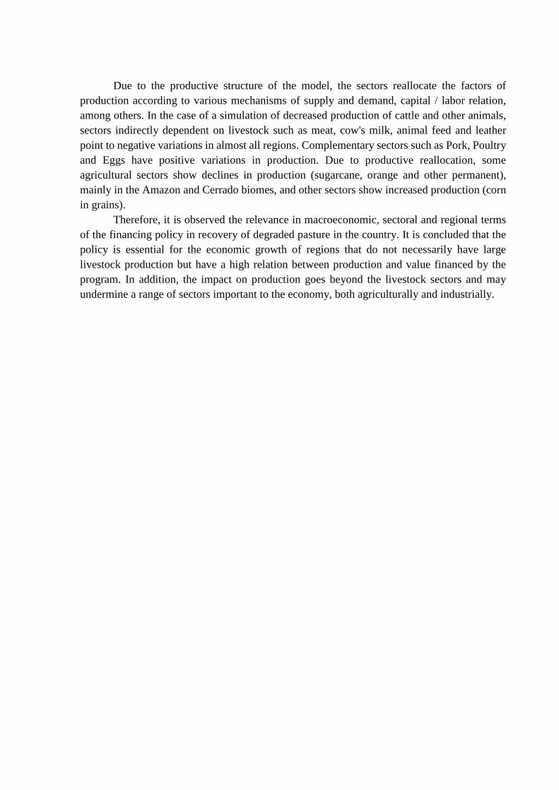
It is also noteworthy that the fall in investment is the biggest driver of the fall in GDP,

followed by the fall in household consumption and exports. The drop in investment is greater

in the Caatinga (SE_Caatinga) and Atlantic Forest (PB_Mata Atlant.) Biomes and is justified

by the low return on capital in these regions. Also noteworthy are the regions of the state of São

Paulo, with significant drops in investment. The regional representation of GDP and investment

follows in the maps of Figures 2 and 3 respectively

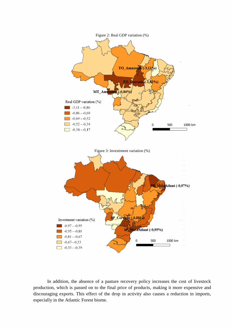
Figure 2: Real GDP variation (%)

Figure 3: Investiment variation (%)

In addition, the absence of a pasture recovery policy increases the cost of livestock

production, which is passed on to the final price of products, making it more expensive and

discouraging exports. This effect of the drop in activity also causes a reduction in imports,

especially in the Atlantic Forest biome.

Employment would also decrease in most regions, suggesting that primary factors of

production (land, capital and labor) become more costly. The fall in employment leads to a

consequent reduction in household income and consumption, indicating that the absence of

policy causes a loss of well-being, especially in the Amazon and Atlantic Forest biome regions.

With the exception of the TO_Amazonia region, which despite the largest drop in GDP pointed

to a positive variation in employment (0.85%), household consumption (0.74%) and imports

(0.57%). This is explained by the reallocation of the factors of production.

Regarding the sectoral results, as expected, the sectoral production of Cattle and Other

Animals was the most affected in all regions, especially TO_Cerrado (-17.9% and -14.3%) and

RR_Amazônia (- 16.2% and -13.3%), the two regions with the largest share of financing for

pasture recovery compared to the production value of the livestock sectors. The Amazon and

Cerrado biomes are the ones that would present the biggest falls in livestock production. Due

to the reallocation of factors of production between sectors and regions, there is an increase in

production in some sectors, especially the Pork, Poultry and Eggs sectors. The swine sector

shows an increase in almost all regions, most significantly in the state of Mato Grosso do Sul,

reaching 0.23% increase in the cerrado biome (MS_Cerrado). The same is true for the Poultry

and Eggs sectors, with increases of 0.28% and 0.26% respectively in the MS_Cerrado region.

Such results can be seen in Table 3 and in the maps of Figures 4 and 5.

Table 3: Result of variation in sectoral output by model region

Regions Cattle Other Animals Swine Poultry Eggs

AC_Amazonia -9.10 -7.84 0.00 -0.03 -0.02

AP_Amazonia -0.28 -1.30 0.03 0.02 -0.02

AM_Amazonia -2.07 -1.16 0.07 0.07 0.03

MA_Amazonia -5.73 -4.31 0.01 -0.05 -0.03

MT_Amazonia -3.52 -3.28 0.17 0.13 0.16

PA_Amazonia -5.80 -5.13 -0.01 -0.11 -0.08

RO_Amazonia -5.77 -4.16 0.06 0.04 0.04

RR_Amazonia -16.20 -13.29 0.00 0.01 0.00

TO_Amazonia -6.80 -6.73 0.03 0.02 0.01

AL_Caatinga -3.08 -1.55 0.10 0.01 0.02

BA_Caatinga -2.80 -1.47 0.17 0.14 0.08

CE_Caatinga -2.23 -0.68 0.03 -0.02 -0.04

MA_Caatinga -2.17 -0.69 0.06 0.07 0.02

MG_Caatinga -2.90 -3.20 0.10 0.10 0.04

PB_Caatinga -3.22 -1.20 0.07 0.03 0.02

PE_Caatinga -2.56 -0.98 0.13 0.06 0.01

PI_Caatinga -2.66 -1.00 0.05 0.03 0.00

RN_Caatinga -3.64 -1.68 0.07 0.00 -0.01

SE_Caatinga -2.18 -0.43 0.11 0.08 0.01

BA_Cerrado -7.23 -4.60 0.02 0.00 -0.02

DF_Cerrado 0.05 0.03 0.15 0.02 -0.01

GO_Cerrado -4.27 -3.70 0.14 0.06 0.06

MA_Cerrado -7.56 -6.38 -0.07 -0.15 -0.08

MT_Cerrado -2.70 -2.32 0.21 0.14 0.09

MS_Cerrado -0.58 -0.99 0.23 0.28 0.27

MG_Cerrado -6.22 -4.26 0.07 -0.03 -0.01

PR_Cerrado -4.95 -3.91 0.16 0.10 0.06

PI_Cerrado -7.54 -5.63 0.00 -0.09 -0.06

SP_Cerrado -1.47 -0.91 0.12 0.05 0.04

TO_Cerrado -17.93 -14.26 -0.18 -0.43 -0.27

AL_Mata Atlant. -2.31 -1.54 0.05 -0.02 -0.06

BA_Mata Atlant. -5.72 -4.58 0.02 -0.10 -0.07

ES_Mata Atlant. -5.91 -4.61 0.13 0.04 0.01

GO_Mata Atlant. -2.00 -1.51 0.16 0.11 0.08

MS_Mata Atlant. -0.34 -0.93 0.22 0.33 0.19

MG_Mata Atlant. -4.52 -2.58 0.14 0.05 0.06

PB_Mata Atlant. -2.06 -1.06 0.02 -0.06 -0.06

PR_Mata Atlant. -2.18 -1.24 0.16 0.14 0.09

PE_Mata Atlant. -2.61 -1.28 -0.03 -0.09 -0.05

RJ_Mata Atlant. -3.14 -1.88 0.09 -0.04 0.02

RN_Mata Atlant. -1.48 -0.70 0.02 -0.03 -0.02

RS_Mata Atlant. -2.50 -0.90 0.15 0.15 0.13

SC_Mata Atlant. -2.54 -0.79 0.12 0.11 0.06

SP_Mata Atlant. -1.61 -1.80 0.08 0.02 0.01

SE_Mata Atlant. -1.34 -0.18 0.05 0.00 -0.02

RS_Pampa -0.93 -0.40 0.20 0.23 0.21

MT_Pantanal -2.07 -3.20 0.12 0.14 0.10

MS_Pantanal 0.32 -0.93 0.20 0.17 0.17

Figure 4: Cattle production variation (%)

Figure 1: Swine production variation (%)

Table 5 in Annex I shows the results of the variation in production across all sectors. In

relation to the agricultural sectors, there is a decrease in production in most sectors and regions,

except for the Corn in Grains sector, which increased mainly in the RS_Pampa (0.14%) and

MS_Cerrado (0.11%) regions. The sectors with the largest production declines were Sugarcane,

Orange and Other Perm. The region with the largest drop in sugarcane production was

TO_Cerrado (-0.41%). In Orange production there is AM_Amazonia (-0.32%) and in

Production of Other Permanent Products in the TO_Cerrado region (-0.42%).

Some industrial sectors also pointed out significant variations. These are the Meat, Cow

Milk, Animal Feed and Leather sectors, all indirectly dependent on livestock or related to

production. It is worth mentioning that the main variations are found in the Amazon and

Cerrado biomes, which are those that received the largest amount of funding in RPD.

5.2 Nationals

Regarding the national results, Chart 2 shows the effects on the main macroeconomic

aggregates. It is possible to see an accumulated fall in almost all households. Investment is

likely to decline most (by almost 1% from the base scenario) due to the fall in capital stock and

consequently low rates of return. The fall in investment and capital stock, coupled with the fall

in household consumption, has a negative impact on GDP of around -0.4% accumulated until

2025. Aggregate employment follows the same trajectory as GDP. Economic growth or decline

implies a greater or lesser use of primary factors in production and there is labor mobility,

reallocating this input sectorally and regionally.

Exports maintain a negative trajectory, with an increase between 2020 and 2022. The

national result is justified by the increase in the cost of livestock production after a shock of

lack of financing for pasture recovery. Such prices are passed on to the final price of the

products, making it more expensive, discouraging exports. Imports follow negative variations,

due to the fall in the activity level, with a slight increase from 2023. Overall, the results point

to relevant economic variations provided by the financing policy of recovering degraded pasture

in the country.

Graph 1: Trajectory of national macroeconomic variables from 2016 to 2025 in the policy scenario

6 CONCLUSION

The main objective of this research was to estimate the regional economic impact of

funding for Plan ABC degraded pasture recovery. For this, a scenario of non-existence of the

policy was simulated between 2016 and 2019 through the fall in livestock activity proportional

to the amount financed by the program during this period. A decrease in production and capital

of livestock sectors is expected to lead to a decrease in the utilization of productive factors and

a reallocation of these factors among other sectors and regions. In addition, the activity level of

some regions and the national economy is expected to decline.

Thus, due to factor reallocation and regional and sectoral interdependence. The results

indicate different impacts between regions and sectors. The greater the representativeness of

the ABC plan financing in relation to the value of production in the livestock sectors, the greater

the accumulated decrease of the region's GDP. Therefore, the absence of financing would cause

a cumulative fall in GDP more sharply in the Amazon and Cerrado biomes, with emphasis on

the TO_Amazonia region, and less markedly in the Pampa, Pantanal and Mata Atlantica

biomes, especially in the MT_Pantanal region.

The reduction in livestock production also causes a decrease in the use of productive

factors and an increase in the production cost of the sector. This mechanism is passed on to the

final price of products, making them more expensive, discouraging exports and causing a

reduction in imports, especially in the Atlantic Forest biome. In addition, there is a decrease in

employment, especially in the regions of the Amazon and Atlantic Forest biome. The

reallocation of labor favors only the TO_Amazonia region. Therefore, the absence of RPD

policy would cause a loss of well-being mainly in the Amazon and Mata Atlantica biomes.

Due to the productive structure of the model, the sectors reallocate the factors of

production according to various mechanisms of supply and demand, capital / labor relation,

among others. In the case of a simulation of decreased production of cattle and other animals,

sectors indirectly dependent on livestock such as meat, cow's milk, animal feed and leather

point to negative variations in almost all regions. Complementary sectors such as Pork, Poultry

and Eggs have positive variations in production. Due to productive reallocation, some

agricultural sectors show declines in production (sugarcane, orange and other permanent),

mainly in the Amazon and Cerrado biomes, and other sectors show increased production (corn

in grains).

Therefore, it is observed the relevance in macroeconomic, sectoral and regional terms

of the financing policy in recovery of degraded pasture in the country. It is concluded that the

policy is essential for the economic growth of regions that do not necessarily have large

livestock production but have a high relation between production and value financed by the

program. In addition, the impact on production goes beyond the livestock sectors and may

undermine a range of sectors important to the economy, both agriculturally and industrially.

ANNEX I

Table 4:BBGEM Model Database Sectors

Sectors

1 Rice 27 Pigmeat 2 Wheat and other cereals 28 Meat Birds 3 Corn grain 29 Industrial Fishing 4 Cotton and other fibers 30 Cold Milk/Pasteurized 5 Sugarcane 31 Other Dairy Products 6 Soybean grain 32 Animal Rations 7 Cassava 33 Food & Beverages 8 Smoke in Leaf 34 Clothing and Textiles 9 Citrus Fruits 35 Footwear and Leather

10 Beans in Grain 36 Wood Product 11 Other Temporary 37 Pulp 12 Orange 38 Diverse Industry 13 Coffee beans 39 Ethanol and Biofuel 14 Other Permanent 40 Chemical 15 Cattle 41 Fertilizer and Fertilizer 16 Other Animals 42 Agricultural And Disinfectant Defensive 17 Cow's Milk 43 Electronic 18 Other Animal Milk 44 Automotive Machines and Equipment 19 Pigs 45 Services 20 Birds 46 Electricity, Gas and Other 21 Eggs 47 Construction 22 Forestry 48 Trade, Wholesale and Retail 23 Plant Extraction 49 Cargo Transport 24 Agricultural Fishing 50 Transportation of Others 25 Extractive Industry 51 Financial and Insurance Institution 26 Beef and Other Animals 52 Public Sector

Fonte: Elaboração própria

Table 5: Result of sectoral output variation by model region (xtot) (%)

Source: Own elaboration based on the research results.

* Caption of sectors according to Table 4 and caption of regions according to Figure 1

Bioma Regiões 1 2 3 4 5 6 7 8 9 10 11 12 13 14 15 16 17 18 19 20 21 22 23 24 25 26 27 28 29 30 31 32 33 34 35 36 37 38 39 40 41 42 43 44 45 46 47 48 49 50 51 52

AC_AM -0.2 -0.2 -0.1 -0.2 -0.4 -0.1 -0.2 -0.1 -0.1 -0.1 -0.1 -0.3 -0.1 -0.3 -9.1 -7.8 -0.1 0.0 0.0 0.0 0.0 -0.2 -0.2 -0.1 -0.2 -1.1 -0.9 -1.0 -3.1 -0.8 -1.3 -0.1 -0.3 -0.4 -0.4 -0.3 -0.1 -0.4 -0.3 -0.3 0.0 -0.1 -0.5 -0.3 -0.3 -0.3 -0.7 -0.4 -0.3 -0.4 -0.5 0.0

AP_AM -0.2 -0.2 0.0 -0.2 -0.4 -0.1 -0.1 -0.1 -0.1 -0.1 -0.1 -0.3 -0.1 -0.4 -0.3 -1.3 0.0 0.0 0.0 0.0 0.0 -0.2 -0.2 -0.1 -0.2 -0.8 -0.7 -0.9 -2.6 -0.4 -0.9 0.0 -0.3 -0.4 -0.4 -0.3 -0.1 -0.4 -0.3 -0.2 -0.1 -0.2 -0.5 -0.4 -0.4 -0.4 -0.7 -0.4 -0.3 -0.5 -0.5 0.0

AM_AM -0.2 -0.2 0.0 -0.2 -0.3 -0.1 -0.1 -0.1 0.0 -0.1 -0.1 -0.3 -0.1 -0.3 -2.1 -1.2 0.1 0.1 0.1 0.1 0.0 -0.2 -0.2 -0.1 -0.3 -0.8 -0.6 -0.7 -2.4 -0.3 -0.8 0.1 -0.3 -0.4 -0.4 -0.2 -0.1 -0.3 -0.3 -0.3 0.0 -0.1 -0.5 -0.3 -0.3 -0.3 -0.8 -0.4 -0.3 -0.4 -0.4 0.0

MA_AM -0.2 -0.2 0.0 -0.2 -0.3 -0.1 -0.1 -0.1 -0.1 -0.1 -0.1 -0.3 -0.1 -0.3 -5.7 -4.3 -0.1 -0.1 0.0 -0.1 0.0 -0.2 -0.2 -0.1 -0.2 -1.0 -0.9 -1.1 -2.8 -0.7 -1.2 0.0 -0.3 -0.4 -0.4 -0.2 -0.1 -0.3 -0.3 -0.3 0.0 -0.1 -0.5 -0.4 -0.3 -0.3 -0.7 -0.3 -0.3 -0.4 -0.4 0.0

MT_AM -0.1 -0.2 0.0 -0.2 -0.3 -0.1 0.0 -0.1 0.0 -0.1 -0.1 -0.2 -0.1 -0.3 -3.5 -3.3 0.1 0.1 0.2 0.1 0.2 -0.1 -0.1 0.1 -0.2 -0.8 -0.6 -0.7 -2.5 -0.4 -0.9 0.3 -0.2 -0.3 -0.4 -0.2 -0.1 -0.2 -0.3 -0.1 0.0 -0.1 -0.4 -0.4 -0.2 0.0 -0.5 -0.4 -0.1 -0.3 -0.3 0.0

PA_AM -0.3 -0.2 -0.1 -0.2 -0.4 -0.1 -0.2 -0.1 -0.1 -0.1 -0.1 -0.3 -0.1 -0.4 -5.8 -5.1 -0.1 0.0 0.0 -0.1 -0.1 -0.2 -0.2 -0.1 -0.1 -1.0 -0.9 -0.9 -3.0 -0.8 -1.2 0.0 -0.4 -0.4 -0.4 -0.3 -0.1 -0.3 -0.4 -0.2 -0.1 -0.2 -0.5 -0.4 -0.4 -0.3 -0.7 -0.4 -0.3 -0.5 -0.5 0.0

RO_AM -0.2 -0.2 0.0 -0.2 -0.3 -0.1 -0.1 -0.1 0.0 -0.1 0.0 -0.2 -0.1 -0.3 -5.8 -4.2 0.0 0.0 0.1 0.0 0.0 -0.2 -0.2 0.0 -0.2 -0.9 -0.7 -0.8 -2.6 -0.5 -1.0 0.0 -0.3 -0.4 -0.4 -0.2 -0.1 -0.3 -0.3 -0.2 0.0 -0.1 -0.4 -0.3 -0.3 -0.3 -0.6 -0.4 -0.2 -0.4 -0.5 0.0

RR_AM -0.2 -0.2 0.0 -0.2 -0.3 -0.1 -0.1 -0.1 0.0 -0.1 -0.1 -0.3 -0.1 -0.4 -16.2 -13.3 -0.1 0.0 0.0 0.0 0.0 -0.2 -0.2 -0.1 -0.2 -1.2 -0.9 -1.0 -2.9 -0.8 -1.3 -0.1 -0.3 -0.4 -0.4 -0.2 -0.1 -0.3 -0.3 -0.3 0.0 -0.1 -0.5 -0.4 -0.4 -0.4 -0.5 -0.3 -0.2 -0.4 -0.5 0.0

TO_AM -0.2 -0.2 0.0 -0.2 -0.3 -0.1 -0.2 -0.1 -0.1 -0.1 -0.1 -0.3 -0.1 -0.3 -6.8 -6.7 0.0 0.0 0.0 0.0 0.0 -0.2 -0.1 -0.1 -0.3 -1.0 -0.9 -1.1 -2.8 -0.7 -1.1 -0.1 -0.3 -0.4 -0.4 -0.2 -0.1 -0.3 -0.3 -0.3 -0.1 -0.2 -0.5 -0.4 -0.1 -0.2 0.0 -0.3 -0.3 -0.4 -0.2 0.0

AL_CA -0.2 -0.2 0.0 -0.1 -0.3 -0.1 -0.1 -0.1 0.0 -0.1 -0.1 -0.3 -0.1 -0.3 -3.1 -1.5 0.0 0.0 0.1 0.0 0.0 -0.2 -0.2 -0.1 -0.3 -0.6 -0.6 -0.5 -2.3 -0.3 -0.8 0.0 -0.3 -0.4 -0.4 -0.2 -0.1 -0.3 -0.3 -0.3 0.0 -0.2 -0.4 -0.3 -0.3 -0.3 -0.7 -0.3 -0.3 -0.4 -0.5 0.0

BA_CA -0.2 -0.2 0.1 -0.1 -0.3 -0.1 -0.1 -0.1 0.0 -0.1 0.0 -0.2 -0.1 -0.3 -2.8 -1.5 0.0 0.0 0.2 0.1 0.1 0.0 -0.1 -0.1 -0.2 -0.6 -0.6 -0.6 -2.3 -0.3 -0.7 0.3 -0.2 -0.4 -0.4 -0.2 -0.1 -0.2 -0.3 -0.1 0.1 0.0 -0.4 -0.3 -0.2 -0.1 -0.5 -0.3 -0.2 -0.3 -0.3 0.0

CE_CA -0.2 -0.2 0.0 -0.2 -0.3 -0.1 -0.1 -0.1 0.0 -0.1 0.0 -0.3 -0.1 -0.3 -2.2 -0.7 -0.1 0.0 0.0 0.0 0.0 -0.2 -0.2 -0.1 -0.3 -0.6 -0.7 -0.5 -2.4 -0.3 -0.7 0.3 -0.3 -0.4 -0.4 -0.3 -0.1 -0.4 -0.3 -0.3 0.0 -0.1 -0.5 -0.4 -0.3 -0.3 -0.8 -0.4 -0.3 -0.4 -0.5 0.0

MA_CA -0.2 -0.2 0.0 -0.1 -0.3 -0.1 -0.1 -0.1 -0.1 -0.1 0.0 -0.2 -0.1 -0.2 -2.2 -0.7 0.0 0.1 0.1 0.1 0.0 -0.2 -0.2 -0.1 -0.1 -0.5 -0.6 -0.5 -2.0 -0.1 -0.6 0.1 -0.3 -0.4 -0.4 -0.2 -0.1 -0.3 -0.3 -0.2 0.0 -0.1 -0.5 -0.4 -0.3 -0.3 -0.7 -0.3 -0.2 -0.4 -0.4 0.0

MG_CA -0.2 -0.2 0.0 -0.2 -0.3 -0.1 -0.1 -0.1 0.0 -0.1 0.0 -0.2 -0.1 -0.3 -2.9 -3.2 0.0 0.1 0.1 0.1 0.0 -0.2 -0.1 -0.1 -0.2 -0.6 -0.6 -0.6 -2.2 -0.2 -0.7 0.0 -0.3 -0.4 -0.4 -0.2 -0.1 -0.3 -0.3 -0.3 0.0 -0.1 -0.5 -0.4 -0.3 -0.3 -0.6 -0.3 -0.3 -0.4 -0.4 0.0

PB_CA -0.2 -0.2 0.0 -0.2 -0.3 -0.1 -0.1 -0.1 0.0 -0.1 0.0 -0.3 -0.1 -0.3 -3.2 -1.2 0.0 0.0 0.1 0.0 0.0 -0.1 -0.2 -0.1 -0.3 -0.7 -0.6 -0.5 -2.3 -0.3 -0.8 0.1 -0.3 -0.4 -0.4 -0.3 -0.1 -0.3 -0.3 -0.3 0.0 -0.2 -0.5 -0.5 -0.3 -0.2 -0.6 -0.3 -0.2 -0.4 -0.4 0.0

PE_CA -0.2 -0.2 0.1 -0.2 -0.3 -0.1 -0.1 -0.1 0.0 -0.1 0.0 -0.2 -0.1 -0.3 -2.6 -1.0 0.0 0.0 0.1 0.1 0.0 0.0 -0.1 -0.1 -0.3 -0.6 -0.6 -0.4 -2.3 -0.3 -0.7 0.5 -0.3 -0.4 -0.4 -0.2 -0.1 -0.3 -0.3 -0.2 0.1 0.0 -0.5 -0.4 -0.3 -0.1 -0.6 -0.3 -0.2 -0.4 -0.4 0.0

PI_CA -0.2 -0.2 0.0 -0.1 -0.3 -0.1 -0.1 -0.1 0.0 -0.1 0.0 -0.2 -0.1 -0.2 -2.7 -1.0 -0.1 0.0 0.1 0.0 0.0 -0.2 -0.2 -0.1 -0.2 -0.7 -0.5 -0.7 -2.3 -0.3 -0.8 0.0 -0.3 -0.4 -0.4 -0.2 -0.1 -0.3 -0.3 -0.3 0.0 -0.1 -0.5 -0.4 -0.2 -0.2 -0.4 -0.3 -0.2 -0.4 -0.4 0.0

RN_CA -0.2 -0.2 0.0 -0.2 -0.3 -0.1 -0.1 -0.1 0.0 -0.1 0.0 -0.2 -0.1 -0.3 -3.6 -1.7 0.0 0.0 0.1 0.0 0.0 -0.2 -0.2 -0.1 -0.3 -0.7 -0.7 -0.8 -2.4 -0.4 -0.8 0.1 -0.3 -0.4 -0.4 -0.3 -0.1 -0.3 -0.3 -0.3 0.0 -0.1 -0.5 -0.5 -0.3 -0.3 -0.7 -0.3 -0.3 -0.4 -0.4 0.0

SE_CA -0.2 -0.2 0.0 -0.1 -0.3 -0.1 -0.1 -0.1 0.0 -0.1 0.0 -0.2 -0.1 -0.3 -2.2 -0.4 -0.1 0.0 0.1 0.1 0.0 -0.2 -0.2 0.0 -0.2 -0.5 -0.5 -0.3 -2.0 -0.2 -0.6 -0.2 -0.3 -0.4 -0.4 -0.1 -0.1 -0.3 -0.3 -0.3 0.0 -0.1 -0.3 -0.3 -0.3 -0.3 -0.5 -0.3 -0.2 -0.4 -0.5 0.0

BA_CE -0.2 -0.2 0.0 -0.2 -0.3 -0.1 -0.2 -0.1 0.0 -0.1 -0.1 -0.3 -0.1 -0.4 -7.2 -4.6 -0.1 0.1 0.0 0.0 0.0 -0.2 -0.2 -0.1 -0.3 -1.0 -0.9 -0.9 -2.9 -0.7 -1.2 -0.1 -0.3 -0.4 -0.4 -0.2 -0.1 -0.3 -0.3 -0.2 0.0 -0.1 -0.5 -0.4 -0.3 -0.3 -0.6 -0.3 -0.2 -0.4 -0.4 0.0

DF_CE -0.2 -0.2 0.0 -0.2 -0.3 -0.1 -0.1 -0.1 0.0 -0.1 0.0 -0.2 -0.1 -0.3 0.0 0.0 0.1 0.1 0.1 0.0 0.0 -0.1 -0.2 -0.1 -0.3 -0.7 -0.6 -0.5 -2.5 -0.4 -0.8 0.0 -0.3 -0.4 -0.4 -0.3 -0.1 -0.4 -0.3 -0.3 0.0 -0.1 -0.5 -0.4 -0.2 -0.3 -0.7 -0.4 -0.3 -0.4 -0.4 0.0

GO_CE -0.2 -0.2 0.0 -0.2 -0.3 -0.1 -0.1 -0.1 0.0 -0.1 -0.1 -0.2 -0.1 -0.4 -4.3 -3.7 0.1 0.0 0.1 0.1 0.1 -0.1 -0.1 0.0 -0.3 -0.9 -0.6 -0.7 -2.7 -0.5 -0.9 0.2 -0.3 -0.4 -0.4 -0.3 -0.1 -0.3 -0.3 -0.3 0.0 -0.1 -0.5 -0.5 -0.3 -0.3 -0.6 -0.4 -0.2 -0.4 -0.4 0.0

MA_CE -0.2 -0.2 -0.1 -0.2 -0.3 -0.1 -0.2 -0.1 -0.1 -0.1 -0.1 -0.3 -0.1 -0.3 -7.6 -6.4 -0.1 -0.1 -0.1 -0.2 -0.1 -0.2 -0.2 -0.1 -0.4 -1.2 -1.0 -1.3 -3.1 -1.0 -1.5 -0.3 -0.3 -0.4 -0.5 -0.3 -0.1 -0.4 -0.3 -0.3 -0.1 -0.2 -0.5 -0.4 -0.3 -0.3 -0.6 -0.4 -0.3 -0.4 -0.4 -0.1

MT_CE -0.1 -0.2 0.0 -0.2 -0.3 -0.1 -0.1 -0.1 0.0 -0.1 0.0 -0.2 -0.1 -0.3 -2.7 -2.3 0.0 0.0 0.2 0.1 0.1 -0.1 -0.2 0.0 -0.3 -0.7 -0.5 -0.4 -2.4 -0.3 -0.7 0.3 -0.3 -0.4 -0.4 -0.2 -0.1 -0.3 -0.3 -0.2 0.0 -0.1 -0.4 -0.4 -0.3 -0.2 -0.5 -0.3 -0.2 -0.3 -0.4 0.0

MS_CE -0.1 0.0 0.1 -0.2 -0.3 -0.1 0.0 -0.1 0.0 -0.1 0.0 -0.2 -0.1 -0.3 -0.6 -1.0 0.2 0.1 0.2 0.3 0.3 0.1 0.0 0.0 -0.2 -0.6 -0.4 -0.4 -2.1 -0.1 -0.5 0.9 -0.2 -0.3 -0.3 -0.1 -0.1 -0.2 -0.3 0.0 0.0 -0.1 -0.4 -0.4 -0.2 0.0 -0.3 -0.2 -0.1 -0.3 -0.3 0.0

MG_CE -0.2 -0.2 0.0 -0.2 -0.3 -0.1 -0.2 -0.1 0.0 -0.1 -0.1 -0.2 -0.1 -0.3 -6.2 -4.3 0.0 0.0 0.1 0.0 0.0 -0.2 -0.2 0.0 -0.3 -1.1 -0.8 -0.9 -2.8 -0.7 -1.1 0.1 -0.3 -0.4 -0.4 -0.3 -0.1 -0.3 -0.3 -0.3 0.0 -0.2 -0.5 -0.5 -0.3 -0.3 -0.7 -0.4 -0.3 -0.4 -0.4 0.0

PR_CE -0.2 -0.1 0.0 -0.2 -0.3 -0.1 -0.1 -0.1 0.0 -0.1 -0.1 -0.2 -0.1 -0.4 -4.9 -3.9 0.1 0.0 0.2 0.1 0.1 -0.2 -0.1 -0.1 -0.3 -0.9 -0.6 -0.6 -2.3 -0.3 -0.8 0.1 -0.3 -0.4 -0.4 -0.3 -0.1 -0.3 -0.3 -0.3 0.0 -0.1 -0.5 -0.5 -0.3 -0.3 -0.8 -0.3 -0.3 -0.4 -0.4 0.0

PI_CE -0.2 -0.2 -0.1 -0.1 -0.3 -0.1 -0.1 -0.1 0.0 -0.1 -0.1 -0.2 -0.1 -0.3 -7.5 -5.6 -0.1 0.0 0.0 -0.1 -0.1 -0.2 -0.2 -0.1 -0.4 -0.9 -0.9 -0.9 -2.7 -0.7 -1.1 -0.1 -0.3 -0.4 -0.4 -0.2 -0.1 -0.4 -0.3 -0.3 0.0 -0.1 -0.5 -0.4 -0.3 -0.3 -0.7 -0.3 -0.3 -0.4 -0.4 0.0

SP_CE -0.2 -0.2 0.0 -0.2 -0.3 -0.1 -0.1 -0.1 0.0 -0.1 0.0 -0.2 -0.1 -0.3 -1.5 -0.9 0.1 0.1 0.1 0.0 0.0 -0.2 -0.1 0.0 -0.4 -0.8 -0.6 -0.6 -2.3 -0.3 -0.8 0.2 -0.3 -0.4 -0.4 -0.3 -0.1 -0.3 -0.3 -0.3 -0.1 -0.2 -0.6 -0.6 -0.3 -0.3 -0.8 -0.4 -0.3 -0.4 -0.4 0.0

TO_CE -0.3 -0.2 -0.4 -0.2 -0.4 -0.2 -0.3 -0.2 -0.1 -0.2 -0.1 -0.3 -0.2 -0.4 -17.9 -14.3 -0.3 -0.1 -0.2 -0.4 -0.3 -0.6 -0.3 -0.2 -0.4 -1.9 -1.5 -1.6 -4.3 -1.9 -2.3 -0.9 -0.4 -0.4 -0.5 -0.4 -0.1 -0.5 -0.4 -0.6 -0.1 -0.2 -0.5 -0.4 -0.4 -0.6 -0.6 -0.6 -0.5 -0.5 -0.6 -0.1

AL_MA -0.2 -0.2 0.0 -0.1 -0.3 -0.1 -0.1 -0.1 -0.1 -0.1 -0.1 -0.3 -0.1 -0.3 -2.3 -1.5 -0.1 0.0 0.1 0.0 -0.1 -0.2 -0.2 -0.1 -0.2 -0.7 -0.6 -0.5 -2.3 -0.3 -0.8 -0.1 -0.3 -0.4 -0.4 -0.2 -0.1 -0.3 -0.3 -0.3 0.0 -0.1 -0.5 -0.4 -0.3 -0.3 -0.8 -0.3 -0.3 -0.4 -0.5 0.0

BA_MA -0.2 -0.2 0.0 -0.1 -0.3 -0.1 -0.1 -0.1 0.0 -0.1 -0.1 -0.3 -0.1 -0.3 -5.7 -4.6 -0.1 0.0 0.0 -0.1 -0.1 -0.2 -0.2 -0.1 -0.2 -1.0 -0.8 -0.8 -2.8 -0.7 -1.2 -0.1 -0.3 -0.4 -0.5 -0.2 -0.1 -0.3 -0.3 -0.3 0.0 -0.2 -0.5 -0.4 -0.3 -0.3 -0.8 -0.4 -0.3 -0.4 -0.5 0.0

ES_MA -0.2 -0.2 0.0 -0.2 -0.3 -0.1 -0.1 -0.1 0.0 -0.1 0.0 -0.3 -0.1 -0.3 -5.9 -4.6 0.0 0.1 0.1 0.0 0.0 -0.2 -0.2 0.0 -0.1 -0.8 -0.6 -0.5 -2.5 -0.4 -0.9 0.0 -0.3 -0.4 -0.4 -0.2 -0.1 -0.3 -0.3 -0.3 0.0 -0.1 -0.5 -0.5 -0.3 -0.3 -0.7 -0.3 -0.3 -0.4 -0.4 0.0

GO_MA -0.2 -0.2 0.0 -0.2 -0.3 -0.1 -0.1 -0.1 0.0 -0.1 0.0 -0.2 -0.1 -0.3 -2.0 -1.5 0.1 0.1 0.2 0.1 0.1 -0.2 -0.1 0.0 -0.2 -0.7 -0.6 -0.6 -2.3 -0.3 -0.7 0.2 -0.3 -0.4 -0.4 -0.2 -0.1 -0.3 -0.3 -0.3 0.0 -0.1 -0.5 -0.4 -0.3 -0.2 -0.6 -0.3 -0.2 -0.3 -0.4 0.0

MS_MA -0.1 -0.1 0.1 -0.2 -0.2 -0.1 0.0 -0.1 0.0 0.0 0.0 -0.2 0.0 -0.3 -0.3 -0.9 0.2 0.1 0.2 0.3 0.2 0.0 0.0 0.0 -0.2 -0.6 -0.4 -0.4 -2.1 -0.1 -0.6 1.0 -0.2 -0.3 -0.3 -0.1 -0.1 -0.2 -0.3 0.0 0.0 -0.1 -0.5 -0.4 -0.2 0.1 -0.5 -0.2 -0.1 -0.3 -0.3 0.0

MG_MA -0.2 -0.2 0.0 -0.2 -0.3 -0.1 -0.1 -0.1 0.0 -0.1 -0.1 -0.2 -0.1 -0.3 -4.5 -2.6 0.1 0.1 0.1 0.1 0.1 -0.2 -0.2 0.0 -0.1 -0.9 -0.7 -0.7 -2.5 -0.4 -0.9 0.1 -0.3 -0.4 -0.4 -0.3 -0.1 -0.3 -0.3 -0.3 0.0 -0.1 -0.6 -0.5 -0.3 -0.3 -0.8 -0.4 -0.3 -0.4 -0.4 0.0

PB_MA -0.2 -0.2 0.0 -0.1 -0.3 -0.1 -0.1 -0.1 0.0 -0.1 0.0 -0.2 -0.1 -0.4 -2.1 -1.1 0.0 -0.1 0.0 -0.1 -0.1 -0.2 -0.2 -0.1 -0.3 -0.7 -0.6 -0.6 -2.3 -0.3 -0.8 0.0 -0.3 -0.4 -0.5 -0.3 -0.1 -0.4 -0.3 -0.3 0.0 -0.1 -0.5 -0.5 -0.3 -0.3 -0.8 -0.4 -0.3 -0.4 -0.5 0.0

PR_MA -0.1 -0.1 0.0 -0.2 -0.3 -0.1 -0.1 -0.1 0.0 -0.1 0.0 -0.2 -0.1 -0.3 -2.2 -1.2 0.1 0.1 0.2 0.1 0.1 -0.1 -0.2 0.0 -0.3 -0.8 -0.6 -0.5 -2.3 -0.3 -0.8 0.3 -0.3 -0.4 -0.4 -0.3 -0.1 -0.3 -0.3 -0.3 0.0 -0.1 -0.5 -0.5 -0.3 -0.2 -0.7 -0.3 -0.3 -0.4 -0.4 0.0

PE_MA -0.2 -0.2 0.0 -0.1 -0.3 -0.1 -0.1 -0.1 0.0 -0.1 0.0 -0.3 -0.1 -0.3 -2.6 -1.3 -0.1 0.0 0.0 -0.1 -0.1 -0.2 -0.2 -0.1 -0.4 -0.7 -0.6 -0.6 -2.3 -0.4 -0.9 0.0 -0.3 -0.4 -0.5 -0.3 -0.1 -0.4 -0.3 -0.4 -0.1 -0.2 -0.6 -0.5 -0.3 -0.3 -0.8 -0.4 -0.3 -0.4 -0.4 0.0

RJ_MA -0.2 -0.2 0.0 -0.2 -0.2 -0.1 -0.1 -0.1 0.0 -0.1 0.0 -0.2 -0.1 -0.3 -3.1 -1.9 0.0 0.0 0.1 0.0 0.0 -0.1 -0.1 0.0 -0.2 -0.8 -0.6 -0.6 -2.4 -0.3 -0.8 0.0 -0.3 -0.4 -0.4 -0.2 -0.1 -0.3 -0.3 -0.3 0.0 -0.1 -0.5 -0.4 -0.3 -0.3 -0.8 -0.3 -0.3 -0.4 -0.4 0.0

RN_MA -0.2 -0.2 0.0 -0.1 -0.3 -0.1 -0.1 -0.1 0.0 -0.1 0.0 -0.3 -0.1 -0.3 -1.5 -0.7 0.0 0.0 0.0 0.0 0.0 -0.1 -0.2 -0.1 -0.2 -0.7 -0.7 -0.7 -2.4 -0.4 -0.8 0.0 -0.3 -0.4 -0.4 -0.3 -0.1 -0.4 -0.3 -0.3 0.0 -0.1 -0.5 -0.5 -0.3 -0.3 -0.8 -0.4 -0.3 -0.4 -0.5 0.0

RS_MA -0.2 -0.1 0.0 -0.2 -0.3 -0.1 -0.2 -0.1 0.0 -0.1 -0.1 -0.2 -0.1 -0.3 -2.5 -0.9 0.1 0.1 0.1 0.2 0.1 -0.2 -0.2 0.0 -0.3 -0.8 -0.5 -0.5 -2.0 -0.2 -0.7 0.3 -0.2 -0.4 -0.4 -0.3 -0.1 -0.3 -0.3 -0.2 0.0 -0.1 -0.6 -0.5 -0.3 -0.2 -0.7 -0.3 -0.2 -0.4 -0.3 0.0

SC_MA -0.2 -0.1 0.0 -0.2 -0.3 -0.1 -0.1 -0.1 0.0 -0.1 0.0 -0.2 -0.1 -0.3 -2.5 -0.8 0.0 0.1 0.1 0.1 0.1 -0.2 -0.2 0.0 -0.3 -0.9 -0.8 -0.6 -2.3 -0.3 -0.8 0.1 -0.3 -0.4 -0.4 -0.2 -0.1 -0.3 -0.3 -0.3 0.0 -0.1 -0.5 -0.5 -0.3 -0.3 -0.8 -0.4 -0.3 -0.4 -0.4 0.0

SP_MA -0.2 -0.2 0.0 -0.2 -0.3 -0.1 -0.1 -0.1 0.0 -0.1 0.0 -0.2 -0.1 -0.4 -1.6 -1.8 0.1 0.1 0.1 0.0 0.0 -0.2 -0.2 0.0 -0.4 -0.9 -0.7 -0.6 -2.3 -0.4 -0.8 0.2 -0.3 -0.4 -0.4 -0.4 -0.1 -0.4 -0.3 -0.3 0.0 -0.2 -0.6 -0.6 -0.3 -0.3 -0.9 -0.4 -0.4 -0.4 -0.4 0.0

SE_MA -0.2 -0.2 0.0 -0.3 -0.3 -0.2 -0.1 -0.1 0.0 -0.1 0.0 -0.3 -0.1 -0.3 -1.3 -0.2 0.0 0.0 0.0 0.0 0.0 -0.2 -0.2 -0.1 -0.2 -0.6 -0.6 -0.5 -2.4 -0.3 -0.8 0.1 -0.3 -0.4 -0.4 -0.2 -0.1 -0.3 -0.3 -0.1 0.0 -0.1 -0.4 -0.4 -0.3 -0.3 -0.6 -0.3 -0.2 -0.3 -0.4 0.0

Pampa RS_PP -0.1 -0.1 0.1 -0.2 -0.3 -0.1 -0.1 -0.1 0.0 -0.1 0.0 -0.2 -0.1 -0.3 -0.9 -0.4 0.2 0.3 0.2 0.2 0.2 -0.1 -0.1 0.0 -0.3 -0.6 -0.5 -0.4 -1.8 -0.2 -0.6 0.9 -0.2 -0.4 -0.4 -0.3 -0.1 -0.3 -0.3 -0.2 0.0 -0.1 -0.6 -0.5 -0.3 -0.2 -0.6 -0.3 -0.2 -0.3 -0.3 0.0

MT_PT -0.1 -0.2 0.0 -0.2 -0.3 -0.1 -0.1 -0.1 0.0 -0.1 0.0 -0.2 -0.1 -0.3 -2.1 -3.2 0.1 0.1 0.1 0.1 0.1 -0.1 -0.1 0.0 -0.2 -0.6 -0.5 -0.5 -2.1 -0.1 -0.6 0.2 -0.2 -0.4 -0.4 -0.2 -0.1 -0.3 -0.3 -0.2 0.0 -0.1 -0.5 -0.3 -0.3 -0.2 -0.5 -0.3 -0.2 -0.4 -0.4 0.0

MS_PT 0.1 -0.2 0.0 -0.2 -0.3 -0.1 -0.1 -0.1 0.0 -0.1 0.0 -0.2 -0.1 -0.3 0.3 -0.9 0.1 0.1 0.2 0.2 0.2 -0.1 -0.1 0.0 -0.1 -0.5 -0.5 -0.4 -2.0 -0.1 -0.5 0.5 -0.3 -0.3 -0.4 -0.2 -0.1 -0.3 -0.3 -0.2 0.0 -0.1 -0.4 -0.3 -0.3 0.0 -0.5 -0.2 -0.1 -0.3 -0.4 0.0

Amazonia

Caatinga

Cerrado

Mata Atlant.

Pantanal

ANNEX II

The core structure of the model database is shown in Figure 2. As in (MAGALHÃES, 2009),

(CARVALHO, 2014), (SOUZA, 2015), (RIBEIRO, 2015), (CARDOSO, 2016) and ( SESSA, 2018),

four final plaintiffs are considered in each region of the model: the representative family (HOU);

capital formation (INV); government demand (GOV), corresponding to the federal, state and

municipal levels; and demand for exports (EXP). In the USE matrix, the values are measured at sales

prices, assuming the possibility that the goods may be re-exported. USE represents product use ratios

(domestic and imported) for 56 users in each of 48 regions: 52 sectors and 4 final plaintiffs

(households, investment, exports, government). The TAX matrix shows the tax revenue per product,

containing elements corresponding to those of the USE matrix.

HOUPUR (c,d)

Valor de compra do produto c usado

pela família representativa em d

Preço: phou(c,d)

Quantidade:xhou_s(c,d)

USER x DST DST ORG x DST

IND FINDEM

COM (HOU,INV,GOV,EXP)

x USE USE_U(c,s,d) DELIVRD(c,s,r,d)

SCR (c,s,u,d) Quantidades: = =

Valor de entrada das semandas : básico + margens xhou(c,s,d) + DELIVRD_R(c,s,d) = CES TRADE(c,s,r,d)

Quantidade: xint(c,s,i,d) xinv(c,s,d) Preço: pdelivrd_r(c,s,d) +

Preço: puse(c,s,d) xgov(c,s,d) Quantidade: xtrad_r(c,s,d) sum{m,MAR,TRADMAR(c,s,m,r,d)

xexp(c,s,d)

Preço: pdelivrd (c,s,r,d)

Demanda final por 4 usuários Quantidade: xtrad (c,s,r,d)

ao preço de entrega puse(c,s,d)

+ = Leontief

COM TAX TRADE

x (c,s,u,d) (c,s,r,d)

SCR Imposto por commodity Produto c,s de r para d a preços básicos

+ Quantidade: xtrad (c,s,r,d)

FACTORS Preço: pbasic(c,s,r)

LAB(i,o,d) salários +

CAP(i,d) aluguel do capital TRADMAR

LND(i,d) remuneração da terra (c,s,m,r,d)

PRODTAX(i,d) produção de impostos Margem m sobre o produto c,s de r para d

= Quantidade: xtradmar (c,s,m,r,d)

Produto da Indústria Preço: psuppmar_p(m,r,d)

VTOT(i,d) Soma sobre COM e SRC

= TRADMAR_CS(m,r,d)

Estoques=STOCKS(i,d) =

+ SUPPMAR_P(m,r,d)

CES soma sobre p em REGPRD

SUPPMAR

MAKE (m,r,d,p)

COM (c,i,d) Soma sobre i em IND = MAKE_I Margem ofertada por p sobre produtos

Produção do bem c pela indústria i em d (c,d) de r para d

Atualização: Oferta de Atualização

xmake(c,i,d)*pdom(c,d) Commodities xsuppmar(m,r,d,p)*pdom(m,p)

domésticas MAKE_I(m,p)=SUPPMAR_RD(m,p)+

TRADE_D(m,"dom",p)

IND x DST DST ORG x DST

MAKE_I

(c,r)

TRADE_D

(c,"dom,r)

These two matrices (USE and TAX), together with the primary factor cost and production tax

matrices, form the production costs (or product value) of each regional industry. In accounting, the

value of each regional industry's product also equals the sum of inventories with the value of each

product's production by each industry in each region (MAKE). Although the production of different

goods by different sectors is possible, the model will be used with the correspondence that each sector

produces only one good, so the MAKE matrix becomes square and diagonal in each region. The

MAKE byproduct, MAKE_I, shows the total output of each product in each target region. This whole

structure is similar to the conventional input-output databases for each region.

The rest of the structure represents the regional supply mechanism. The regional origin of the

goods is informed by the TRADE matrix, which represents the flow of trade between the regions for

each of the 52 products in the model, both domestic and imported. The diagonal of this matrix shows

the value of local usage that is offered locally. In the case of imported products, regional origin is the

port of entry into the country. And the IMPORT matrix lists the total imports by each port, simply

being an aggregation of the TRADE matrix import share. The TRADMAR matrix presents the margin

value required to carry out the trade flows of each TRADE matrix element, but without any inference

as to where the margin flow is produced. The sum of the TRADE and TRADMAR matrices gives rise

to the “delivery” price of all product flows (DELIVRD).

The origin of margins is presented in the SUPPMAR matrix, regardless of the products or their

origin, domestic or imported, so that the total use of margins to market or transport any product from

one region to another follows the same proportion. The sum of the regional margins forms the matrix

SUPPMAR_P, which has the same value as TRADMAR_CS, derived from the TRADMAR matrix

from the margins of domestic and imported products. In this structure, TRADMAR_CS is an

aggregation of SUPPMAR from a constant substitution elasticity (CES) function, and thus the margins

for a given product on a given route are set according to the price of that margin in the various regions.

In the model, all users of a given good in a region have the same source mix, adopting the

Armington substitution, where the DELIVRD_R matrix is a CES compound of the DELIVRD matrix.

The existence of equilibrium depends on the sum of USE (USE_U) being equal to the sum of

DELIVRD (DELIVRD_R).

Compatibility between supply and demand for household goods occurs between the MAKE_I

matrix and the TRADE and SUPPMAR matrices. For non-margin products, the domestic elements

contained in the TRADE matrix are added to the corresponding elements in the MAKE_I commodity

supply matrix. And in the case of margin assets, the margin requirements of matrix SUPPMAR_RD

and the direct demand presented in matrix TRADE_D are considered.

Investments are divided according to the destination industry or import entry point in the

INVEST matrix.

In addition to the data presented so far, the BBGEM model needs behavioral parameters and

elasticities, which are usually found in other studies in the literature. The main parameters of the model

are: intermediate goods substitution elasticity (ARMSIGMA), substitution elasticity between regions

(SIGMADOMDOM), household spending elasticity (EPS), export demand elasticities

(EXP_ELAST). CET transformation elasticities (SIGMAOUT) and CES substitution elasticity for

primary factors (SIGMA1PRIM). For the elasticity calibration, the estimates of (FARIA and

HADDAD, 2014), (KUME and PIANI, 2013), (TOURINHO, KUME and PEDROSO, 2007) and

(HOFFMANN, 2010) were used. These estimates are the most recent found in the literature. It is

noteworthy that the elasticity values had to be adjusted according to BBGEM's sectoral and regional

structure.

REFERENCES

BARROS, A. M. DE. Avaliação do uso estratégico das áreas prioritárias do Programa ABC. [s.l.]

Observatório ABC, 2017.

BRASIL. MINISTÉRIO DA AGRICULTURA, PECUÁRIA E ABASTECIMENTO (MAPA). Plano

setorial de mitigação e de adaptação às mudanças climáticas para a consolidação de uma economia

de baixa emissão de carbono na agricultura : plano ABC (Agricultura de Baixa Emissão de

Carbono). Brasília, 2012.

BRASIL. MINISTÉRIO DA AGRICULTURA, PECUÁRIA E ABASTECIMENTO (MAPA).

Projeções do Agronegócio : Brasil 2018/19 a 2028/29 projeções de longo prazo. Secretaria de

Política Agrícola. – Brasília, 2019. 126 p.

CARVALHO, L. R., JUNIOR, A. A. B., DO AMARAL, P. V. M., & DOMINGUES, E. P. Matrizes

de distâncias entre os distritos municipais no Brasil: um procedimento metodológico. Texto para

Discussão, (532). 2016.

CARVALHO, T. S. Uso do Solo e Desmatamento nas Regiões da Amazônia Legal Brasileira:

condicionantes econômicos e impactos de políticas públicas. Universidade Federal de Minas Gerais

(UFMG) - Tese de Doutorado. Belo Horizonte, p. 219. 2014.

CARDOSO, D. F. Capital e Trabalho no Brasil no Século XXI: Impacto de Políticas de

Transferência e de Tributação sobre a Desigualdade, Consumo e Estrutura Produtiva. Universidade

Federal de Minas Gerais. Belo Horizonte, p. 274. 2016

DIXON, P. B. et al. ORANI: A Multisectoral Model of the Australian Economy. Amsterdam: North-

Holland, 1982.

DIXON, P.B.; PARMENTER, B.R.; RYLAND, G.J.; SUTTON, J.M. ORANI: A General

Equilibrium Model of the Australian Economy, Contributions to Economic Analysis, North-Holland

Publishing Company. 1982.

DIXON, P.; RIMMER, M. Dynamic general equilibrium modelling for forecasting and policy. A

practical guide and documentation of MONASH. Cayton: Emerald, 2002.

DIXON, P.B.; KOOPMAN, R. B.; RIMMER, M. T. The MONASH Style of Computable General

Equilibrium Modeling: A Framework for Practical Policy Analysis. In: DIXON, P.B.; JORGESON,

D (Ed). W. Handbook of CGE modeling. Oxford: Elsevier, 2013, v.1.

DOMINGUES, E. P. Dimensão regional e setorial da integração brasileira na Área de Livre

Comércio das Américas. São Paulo: Universidade de São Paulo, 2002. Tese de Doutorado. 223p.

DOMINGUES, E. P.; BETARELLI A. A. J.; MAGALHÃES, A. S.; OLIVEIRA, H. C.;

VALLADARES, L.M.. Calibragem do Modelo ORANIG para os Dados da Matriz InsumoProduto

Nacional (2005). Relatório Técnico de Pesquisa. CEDEPLAR/UFMG, 2009, 33 p.

FARIA, W. R.; HADDAD, E. A. Estimação das elasticidades de substituição do comércio regional

do Brasil. Nova Economia, Belo Horizonte, v. 24, n. 1, p. 141-168, Janeiro-Abril 2014

FOCHEZATTO, A. Construção de um modelo de equilíbrio geral computável regional: aplicação ao

Rio Grande do Sul. Instituto de Pesquisa Econômica Aplicada (IPEA). Brasília, p. 29. 2003.

HADDAD, E. A. Retornos crescentes, custos de transporte e crescimento regional. – Faculdade de

Economia, Administração e Contabilidade da Universidade de São Paulo (FEA/ USP), São Paulo,

2004. (Tese de Livre-Docência em Economia).

HARRISON, W. J.; PEARSON, K. R. Computing solutions for large general equilibrium models

using GEMPACK. Computational Economics, v. 9, n. 2, p. 83–127, Agosto 1996.

HASEGAWA, M. M. Políticas Públicas na Economia Brasileira: uma aplicação do modelo MIBRA,

um modelo interregional aplicado de equilíbrio geral. Escola Superior de Agricultura Luis de

Queiroz (ESALQ/USP) - Tese de Doutorado. Piracicaba, p. 300. 2003

HOFFMANN, R. Estimativas das Elasticidades-Renda de Várias Categorias de Despesa e de

Consumo, Especialmente Alimentos, no Brasil, com base na POF 2008-2009. Revista de Economia

Agrícola, São Paulo, v. 57, n. 2, p. 49-62, Julho-Dezembro 2010.

HORRIDGE, J. M. Preparing a TERM bottom-up regional database. Centre of Policy Studies. [S.l.].

2006.

HORRIDGE, J. M.; MADDEN, J. R.; WITTWER, G. The impact of the 2002-03 drought on

Australia. Journal of Policy Modeling, v. 27, n. 3, p. 285–308, 2005.

HORRIDGE J.M., JERIE M., MUSTAKINOV D. & SCHIFFMANN F. GEMPACK manual,

GEMPACK Software, ISBN 978-1-921654-34-3. 2018.

INSTITUTO BRASILEIRO DE GEOGRAFIA (IBGE). Matriz de insumo-produto – Brasil - 2015.

Coordenação de Contas Nacionais. -Rio de Janeiro, 2018. 60p. – (Contas nacionais, ISSN 1415-9813

; n. 62)

INSTITUTO BRASILEIRO DE GEOGRAFIA (IBGE). Censo agropecuário 2006.. IBGE, 2006.

KUME, H.; PIANI, G. Elasticidades de Substituição das Importações no Brasil. Revista de

Economia Contemporânea, Rio de Janeiro, v. 17, n. 3, p. 423-451, Setembro-Dezembro 2013.

MAGALHÃES, A. S. O comércio por vias internas e seu papel sobre crescimento e desigualdade

regional no Brasil. Universidade Federal de Minas Gerais (UFMG) - Dissertação de Mestrado. Belo

Horizonte, p. 134. 2009.

MAGALHÃES, A. S. Economia de baixo carbono no Brasil: alternativas de políticas e custos de

redução de emissões de gases de efeito estufa. Universidade Federal de Minas Gerais (UFMG) - Tese

de Doutorado. Belo Horizonte, p. 290. 2013.

OBSERVATÓRIO ABC. Análise dos Recursos do Programa ABC Safra 2016 / 17 Observatório do

Plano ABC ( Contribuição para a NDC e Capacita ABC ). p. 1–36, 2017a.

OBSERVATÓRIO ABC. Impactos econômicos e ambientais do Plano ABC. p. 1–28, 2017b.

OCDE‐FAO. Agricultural Outlook 2015-2024. OECD Publishing, 2015.

PEREIRA, S., E., M., et al. Análise multicritério para planejamento em sistemas de integração

lavoura, pecuária e floresta. Jaguariúna: Embrapa Meio Ambiente, 2018.

PETER, W. W. HORRIDGE, M.; MEGUER, G.A. NAVQUI, F.; PARMENTER, B. R. The

theoretical structure of MONASH-MRF. Cayton: Center of Policy Studies, 1996. 121 p. (Preliminary

working paper, OP-85)

RIBEIRO, L. C. D. S. Investimentos Estruturantes e Desigualdades Regionais na Região Nordeste.

Universidade Federal de Minas Gerais (UFMG) - Tese de Doutorado. Belo Horizonte, p. 205. 2015

SESSA, C. B. Comércio exterior, guerra fiscal e dinâmica regional assimétrica no brasil e no espírito

santo. Universidade Federal de Minas Gerais (UFMG) – Tese de doutorado. Belo Horizonte, p. 237.

2018.

SIMONATO, T. C.. Avaliação dos Impactos economicos do desastre minerário de MarianaMG.

Dissertação (Economia) - Universidade Federal de Minas Gerais. 2016.

SOUZA, K. B. Impactos econômicos da participação da mulher no mercado de trabalho brasileiro:

uma análise de equilíbrio geral. Universidade Federal de Minas Gerais. Belo Horizonte, p. 160. 2015.

TOURINHO, O. A. F.; KUME, H.; PEDROSO, A. C. D. S. Elasticidades de Armington para o

Brasil: 1986-2002. Revista Brasileira de Economia, Rio de Janeiro, v. 61, n. 2, p. 245–267, Abril-

Junho 2007