The Perth Photochemical Smog Study monitoring network · 2016-01-21 · The Perth Photochemical...

The Perth Photochemical Smog Study monitoring network

Arthur Grieco, Peter Mountford and Robert Kleinfelder

Department of Environmental Protection Perth, Western Australia

Technical Series 82 May 1996

ISBN. 0 7309 5783 7 ISSN. 1030 –0600

i

Contents

Figures ...................................................................................................................................... iv

Tables......................................................................................................................................... v

1. Introduction .......................................................................................................................... 1

2. Location of monitoring stations........................................................................................... 1

3. Overview of air quality monitoring stations ...................................................................... 1

4. Logging and telemetry instrumentation ............................................................................. 5

4.1. Data logger....................................................................................................................... 5 4.2. Telemetry system............................................................................................................. 6

5. Air quality instrumentation................................................................................................. 7

5.1. Chart recorder .................................................................................................................. 7 5.2. Sample inlet system ......................................................................................................... 7 5.3. Ozone monitor ................................................................................................................. 9

5.3.1. Nature and sources................................................................................................. 9 5.3.2. Monitor type ........................................................................................................ 10 5.3.3. Measurement principle ........................................................................................ 10

5.4. Oxides of nitrogen ......................................................................................................... 10

5.4.1. Nature and sources............................................................................................... 10 5.4.2. Monitor type ........................................................................................................ 10 5.4.3. Measurement principle ........................................................................................ 10

5.5. Carbon monoxide .......................................................................................................... 11

5.5.1. Nature and sources............................................................................................... 11 5.5.2. Monitor used........................................................................................................ 11 5.5.3. Measurement principle ........................................................................................ 11

5.6. Sulphur dioxide ............................................................................................................. 12


5.7. Particulates..................................................................................................................... 13


ii

5.8. Hydrocarbons................................................................................................................. 15


5.9. Photochemical smog...................................................................................................... 16

6. Meteorological instrumentation ........................................................................................ 16

6.1. Wind speed and direction .............................................................................................. 16 6.2. Air temperature.............................................................................................................. 17 6.3. Temperature lapse rate................................................................................................... 17 6.4. Relative humidity........................................................................................................... 17 6.5. Radiation........................................................................................................................ 17 6.6. Air pressure.................................................................................................................... 18 6.7. Rainfall .......................................................................................................................... 18

7. Upper air profiling instrumentation ................................................................................. 18

7.1. Remote sensing.............................................................................................................. 18 7.1.1. Rass radar ............................................................................................................ 18 7.1.2. Sodars .................................................................................................................. 20

7.2. Radiosonde program...................................................................................................... 22

8. Calibration and maintenance procedures ........................................................................ 23

8.1. Australian & US standards ............................................................................................ 23 8.1.1. Air quality measurement standards...................................................................... 23 8.1.2. Meteorological measurement standards .............................................................. 24

8.2. Calibration procedures................................................................................................... 24

8.2.1. Air quality monitor calibration procedures.......................................................... 24 8.2.2. Meteorological measurement calibration procedures .......................................... 24

8.3. Preventative maintenance .............................................................................................. 25

8.3.1. Air quality monitoring equipment ....................................................................... 26 8.3.2. Meteorological equipment ................................................................................... 26

8.4 Control charts ................................................................................................................. 27

9. Data processing ................................................................................................................... 28

9.1. Chemical data processing .............................................................................................. 28 9.2. Meteorological data processing ..................................................................................... 29

iii

9.3. Daily data validation...................................................................................................... 30 9.4. Data storage and access ................................................................................................. 31

9.4.1. Description of data bases ..................................................................................... 31 9.4.2. Accessing the data bases...................................................................................... 31 9.4.3. Data report ........................................................................................................... 31

10. References.......................................................................................................................... 34

iv

Figures

Figure 2.1 - Locations of measurement sites used for the Perth Photochemical Smog Study.... 2

Figure 3.1 - Air quality monitoring shed at Caversham. ............................................................ 5

Figure 4.1 - Shed interior showing IBM compatible PC, strip chart recorder and logger. ......... 6

Figure 4.2 - Monitoring shed data flow diagram. ....................................................................... 7

Figure 5.1 - Equipment sample line schematic........................................................................... 8

Figure 5.2 - Shed interior showing an ozone monitor with the site log book............................. 9

Figure 5.3 - General schematic of an ultraviolet photometric ozone monitor. ........................... 9

Figure 5.4 - General schematic of a NOx monitor. .................................................................. 11

Figure 5.5 - General schematic of a CO monitor...................................................................... 12

Figure 5.6 - Energy diagram of an excited SO2 molecule........................................................ 13

Figure 5.7 - Nephelometer mounting........................................................................................ 13

Figure 5.8 - TEOM on a metal base. ........................................................................................ 13

Figure 5.9 - High volume sampler with a TSP head................................................................. 14

Figure 5.10 - High volume sampler with a PM10 head............................................................ 14

Figure 5.11 - General schematic of an integrating nephelometer optical chamber. ................. 15

Figure 6.1 - Meteorological equipment on a 10 metre guyed tower........................................ 17

Figure 7.1 - Radian LAP3000 model RASS located at Cullacabardee. ................................... 19

Figure 7.2 - Sodar compound located at Cullacabardee. .......................................................... 20

Figure 7.3 - Sodar equipment located at Gidgegannup. ........................................................... 21

Figure 7.4 - Frequency of valid wind velocity measurements made by the Cullacabardee sodar, for both 10 minute and 30 minute averaging intervals. ......................................... 21

Figure 7.5 - Releasing a sonde balloon..................................................................................... 23

Figure 8.1 - Control chart for the ozone monitor at Swanbourne............................................. 27

Figure 9.1 - Sample raw data file.............................................................................................. 28

Figure 9.2 - Sample calibration file. ......................................................................................... 28

Figure 9.3 - Sample plot showing an elevated baseline, calibration and power failure. .......... 30

Figure 9.4 - Sample data base plot............................................................................................ 32

Figure 9.5 - Sample monthly report.......................................................................................... 33

v

Tables 3.1 - Parameters measured at each site in the Perth Photochemical Smog Study................... 3

3.2 - Periods of operation of Perth Photochemical Smog Study sites..................................... 4

8.1 - Air quality monitoring preventative maintenance schedule.......................................... 26

9.1 - Flag definitions as used in the calibration files............................................................. 30

1

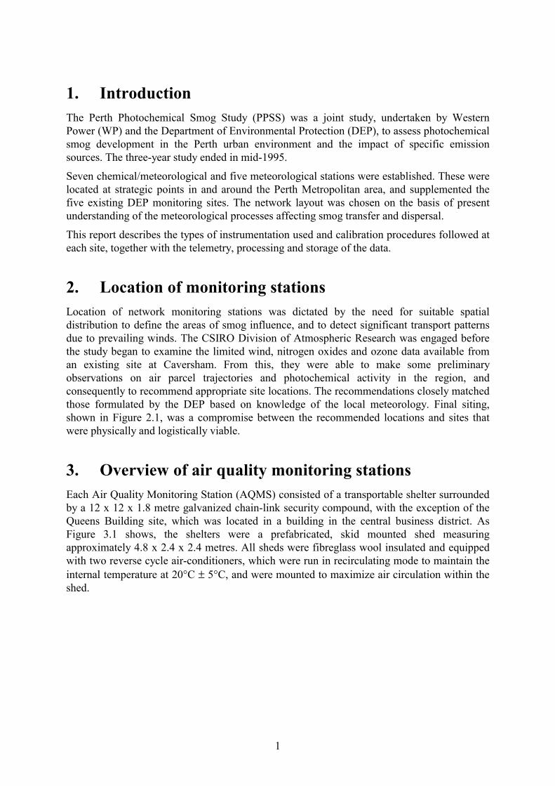
1. Introduction The Perth Photochemical Smog Study (PPSS) was a joint study, undertaken by Western Power (WP) and the Department of Environmental Protection (DEP), to assess photochemical smog development in the Perth urban environment and the impact of specific emission sources. The three-year study ended in mid-1995.

Seven chemical/meteorological and five meteorological stations were established. These were located at strategic points in and around the Perth Metropolitan area, and supplemented the five existing DEP monitoring sites. The network layout was chosen on the basis of present understanding of the meteorological processes affecting smog transfer and dispersal.

This report describes the types of instrumentation used and calibration procedures followed at each site, together with the telemetry, processing and storage of the data.

2. Location of monitoring stations Location of network monitoring stations was dictated by the need for suitable spatial distribution to define the areas of smog influence, and to detect significant transport patterns due to prevailing winds. The CSIRO Division of Atmospheric Research was engaged before the study began to examine the limited wind, nitrogen oxides and ozone data available from an existing site at Caversham. From this, they were able to make some preliminary observations on air parcel trajectories and photochemical activity in the region, and consequently to recommend appropriate site locations. The recommendations closely matched those formulated by the DEP based on knowledge of the local meteorology. Final siting, shown in Figure 2.1, was a compromise between the recommended locations and sites that were physically and logistically viable.

3. Overview of air quality monitoring stations Each Air Quality Monitoring Station (AQMS) consisted of a transportable shelter surrounded by a 12 x 12 x 1.8 metre galvanized chain-link security compound, with the exception of the Queens Building site, which was located in a building in the central business district. As Figure 3.1 shows, the shelters were a prefabricated, skid mounted shed measuring approximately 4.8 x 2.4 x 2.4 metres. All sheds were fibreglass wool insulated and equipped with two reverse cycle air-conditioners, which were run in recirculating mode to maintain the internal temperature at 20°C ± 5°C, and were mounted to maximize air circulation within the shed.

2

Monitoring equipment, together with an IBM compatible 386SX personal computer and a strip chart recorder, was arranged along benches in each shed. Pollutants monitored included one or more of ozone, nitric oxide, nitrogen dioxide, carbon monoxide, sulphur dioxide and hydrocarbons. A typical shed interior is shown in Figures 4.2 and Figure 5.3.

At selected sites a nephelometer, used for measuring the visibility reduction attributable to airborne particulates, was fixed to an internal wall of the shed as shown in Figure 5.7. In addition a tapered element oscillating microbalance (TEOM) monitor was mounted on a metal based stand passing through the shed floor into a buried concrete block to isolate it from vibrations (see Figure 5.8). Most sites also included a 10 metre tall tower to support the wind speed and direction and temperature sensors (Figure 6.1), with Caversham and Hope Valley having 18 metre and 27 metre towers respectively.

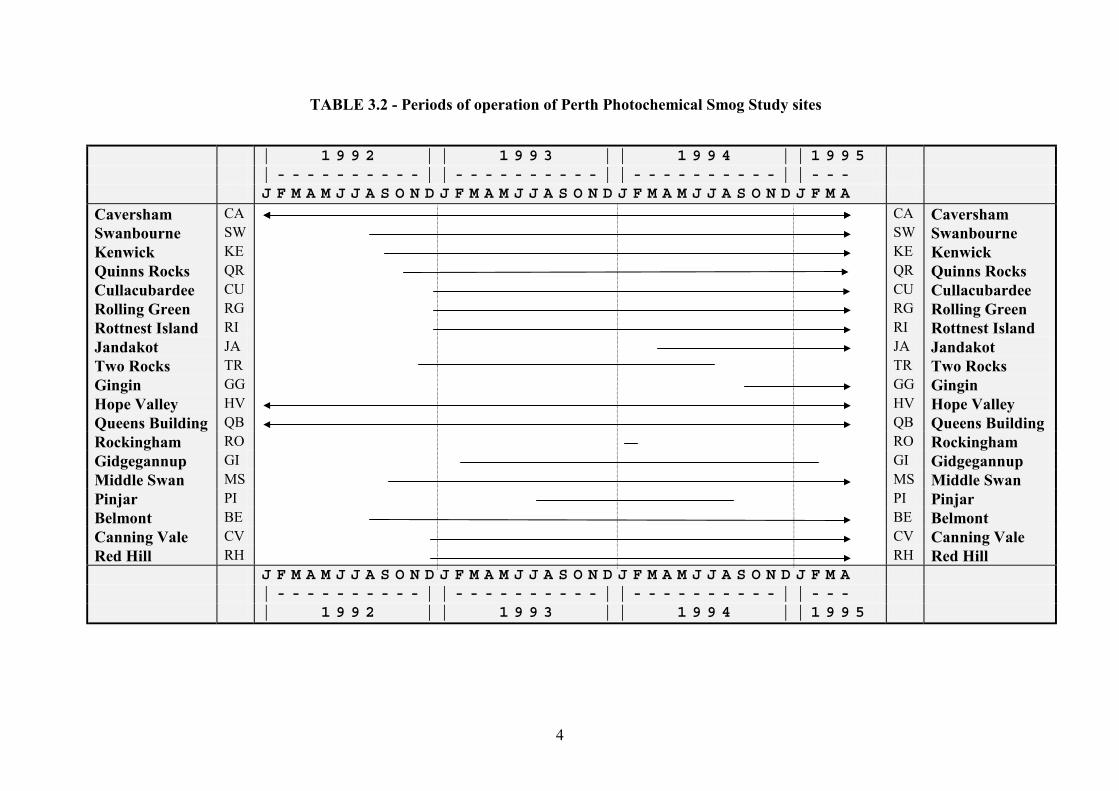
Table 3.1 shows the variables measured at each site and the date operations began and Table 3.2 summarises the periods of operation of each site.

Rottnest Island

Swanbourne

Quinns Rocks

Two Rocks

Queens Buildings

Caversham

Kenwick

Rolling Green

Hope Valley

Cullacabardee

North Rockingham

Belmont

Canning Vale

Gidgegannup

Middle Swan Red Hill

Jandakot

PinjarTiwest Chandala

Ocean Reef

Mount Lawley

0 5 10 15 20Scale (km)

KEYAQMS Sites

Meteorology only

Bureau of Met.

RadarSodar

Gingin

Duncraig

Figure 2.1 - Locations of measurement sites used for the Perth Photochemical Smog Study.

3

TABLE 3.1 - Parameters measured at each site in the Perth Photochemical Smog Study

SITE site Parameters Measured

code year O3 NOx SO2 CO H/C TSP VISI PM25 PM10 WS10 WD10 AT10 DELT NR SR UV RAIN PRES RH10 ATRK SODR RASS

Caversham CA 10/89 • • • • • • • • • • • • • • • • •Swanbourne SW 08/92 • • • • • • • • • • • Kenwick KE 09/92 • • • • • • • • • Quinns Rocks QR 10/92 • • • • • Cullacubardee CU 12/92 • • • • • • • • • •Rolling Green RG 12/92 • • • • • Rottnest Island RI 12/92 • • • • • • Jandakot JA 03/94 • • • • • • Two Rocks TR 11/92 • • • • • Gingin GG 08/94 • • • • • Hope Valley HV 01/89 • • • • • • • • • • • • Queens Building QB 07/89 • • • • • • Rockingham RO 10/91 • • • Gidgegannup GI 02/93 • • • • Middle Swan MS 09/92 • • • Pinjar PI 07/93 • • • Belmont BE 08/92 • • • Canning Vale CV 12/92 • • • Red Hill RH 12/92 • • •

Note : Symbols used are:

PARAMETER PARAMETER DESCRIPTION MANUFACTURER MODEL METHOD O3 ozone Thermo Environmental Instruments TE 49 Ultraviolet absorption NOx nitric oxide and nitrogen dioxide Thermo Environmental Instruments TE 42 Chemiluminescence SO2 sulphur dioxide Monitor Labs 8850S Ultraviolet fluorescence CO carbon monoxide Thermo Electron Corporation TE 48 Gas filter correlation H/C hydrocarbons Horiba Ltd. APHA-350E Flame ionization TSP total suspended particulates Cairns Instrument Services Mk3 High volume sampler VISI visibility Belfort Instrument Company 1591 Integrating nephelometer PM2.5 sub 2.5 micron particles Rupprecht & Patashnick 1400a Tapered element oscillating microbalance (TEOM) PM10 sub 10 micron particles Cairns Instrument Services Mk3 High volume sampler with size selective head WS10 wind speed at 10 metres Climatronics WMIII 3 cup anemometer WD10 wind direction at 10 metres Climatronics WMIII Wind vane with single potentiometer AT10 air temperature at 10 metres Unidata 6507 Thermistor, non-aspirated DELT delta temperature DEP - Electronic subtraction NR net radiation Middleton CN1 Net pyrradiometer SR solar radiation Eppley 8-48 Black and white pyranometer UV ultra violet radiation Eppley TUVR Selenium PE cell RAIN rain Rimco 491001 Tipping bucket RH10 relative humidity Rotronics MP100 Hygromer PRES atmospheric pressure Vaisala PTA427 Barocap silicon capacitive gauge ATRK smog monitor Mineral Control Instrumentation Airtrak 2000 Chemiluminescence SODR wind profile Australian Defence Academy Mk4 Doppler acoustic sounder RASS wind and temperature profile Radian Lap3000 915MHz doppler radar and RASS

4

TABLE 3.2 - Periods of operation of Perth Photochemical Smog Study sites

| 1 9 9 2 | | 1 9 9 3 | | 1 9 9 4 | | 1 9 9 5 | - - - - - - - - - - | | - - - - - - - - - - | | - - - - - - - - - - | | - - - J F M A M J J A S O N D J F M A M J J A S O N D J F M A M J J A S O N D J F M A Caversham CA CA Caversham Swanbourne SW SW Swanbourne Kenwick KE KE Kenwick Quinns Rocks QR QR Quinns Rocks Cullacubardee CU CU Cullacubardee Rolling Green RG RG Rolling Green Rottnest Island RI RI Rottnest Island Jandakot JA JA Jandakot Two Rocks TR TR Two Rocks Gingin GG GG Gingin Hope Valley HV HV Hope Valley Queens Building QB QB Queens Building Rockingham RO RO Rockingham Gidgegannup GI GI Gidgegannup Middle Swan MS MS Middle Swan Pinjar PI PI Pinjar Belmont BE BE Belmont Canning Vale CV CV Canning Vale Red Hill RH RH Red Hill J F M A M J J A S O N D J F M A M J J A S O N D J F M A M J J A S O N D J F M A | - - - - - - - - - - | | - - - - - - - - - - | | - - - - - - - - - - | | - - - | 1 9 9 2 | | 1 9 9 3 | | 1 9 9 4 | | 1 9 9 5

5

4. Logging and telemetry instrumentation

4.1. Data logger Data logging at each site was done by a Unidata STARLOG Macro data logger with a memory capacity of 64 kilobytes. Once a second, the data acquisition read the voltages generated by the air quality and meteorological equipment at the site. Internal processing by the logger generated a ten minute average for each parameter. This value was then stored in the logger's memory. Depending on the number of parameters measured at each site, a logger's memory filled within a period ranging from two weeks to two months. Any new data collected after the logger’s memory has been filled overwrite the oldest data in the logger’s memory.

Figure 3.1 - Air quality monitoring shed at Caversham.

6

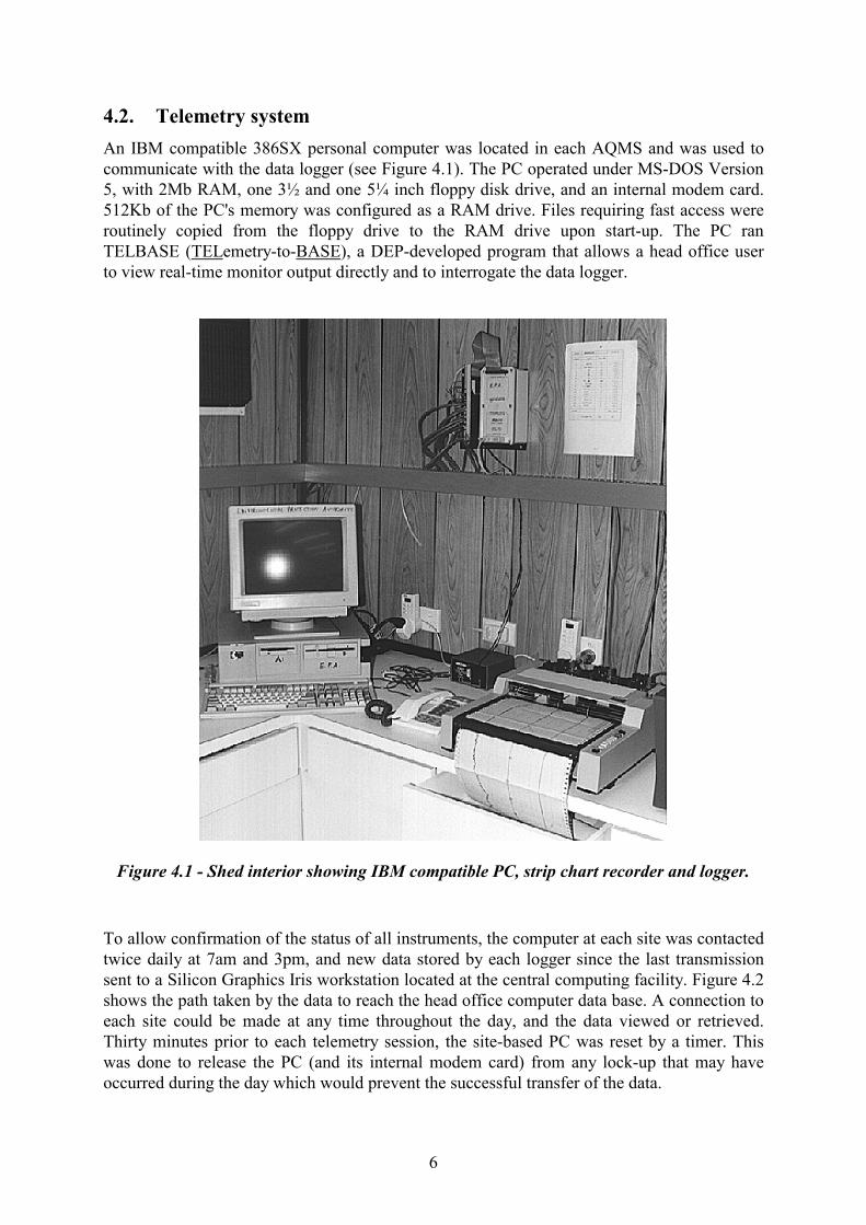
4.2. Telemetry system An IBM compatible 386SX personal computer was located in each AQMS and was used to communicate with the data logger (see Figure 4.1). The PC operated under MS-DOS Version 5, with 2Mb RAM, one 3½ and one 5¼ inch floppy disk drive, and an internal modem card. 512Kb of the PC's memory was configured as a RAM drive. Files requiring fast access were routinely copied from the floppy drive to the RAM drive upon start-up. The PC ran TELBASE (TELemetry-to-BASE), a DEP-developed program that allows a head office user to view real-time monitor output directly and to interrogate the data logger.

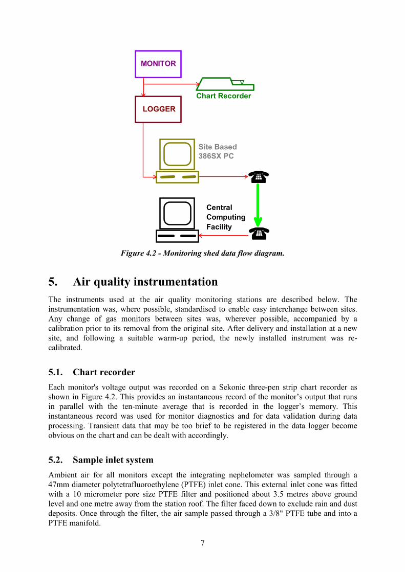
To allow confirmation of the status of all instruments, the computer at each site was contacted twice daily at 7am and 3pm, and new data stored by each logger since the last transmission sent to a Silicon Graphics Iris workstation located at the central computing facility. Figure 4.2 shows the path taken by the data to reach the head office computer data base. A connection to each site could be made at any time throughout the day, and the data viewed or retrieved. Thirty minutes prior to each telemetry session, the site-based PC was reset by a timer. This was done to release the PC (and its internal modem card) from any lock-up that may have occurred during the day which would prevent the successful transfer of the data.

Figure 4.1 - Shed interior showing IBM compatible PC, strip chart recorder and logger.

7

5. Air quality instrumentation The instruments used at the air quality monitoring stations are described below. The instrumentation was, where possible, standardised to enable easy interchange between sites. Any change of gas monitors between sites was, wherever possible, accompanied by a calibration prior to its removal from the original site. After delivery and installation at a new site, and following a suitable warm-up period, the newly installed instrument was re-calibrated.

5.1. Chart recorder Each monitor's voltage output was recorded on a Sekonic three-pen strip chart recorder as shown in Figure 4.2. This provides an instantaneous record of the monitor’s output that runs in parallel with the ten-minute average that is recorded in the logger’s memory. This instantaneous record was used for monitor diagnostics and for data validation during data processing. Transient data that may be too brief to be registered in the data logger become obvious on the chart and can be dealt with accordingly.

5.2. Sample inlet system

Ambient air for all monitors except the integrating nephelometer was sampled through a 47mm diameter polytetrafluoroethylene (PTFE) inlet cone. This external inlet cone was fitted with a 10 micrometer pore size PTFE filter and positioned about 3.5 metres above ground level and one metre away from the station roof. The filter faced down to exclude rain and dust deposits. Once through the filter, the air sample passed through a 3/8" PTFE tube and into a PTFE manifold.

MONITOR

LOGGER

Site Based386SX PC

CentralComputingFacility

Chart Recorder

Figure 4.2 - Monitoring shed data flow diagram.

8

As shown in Figure 5.1, the O3 monitor draws its air directly from this internal manifold through a short length of 1/4" polyfluoroacetate (PFA) tube. The remaining instruments (NOx, CO and SO2) draw their sample air from the internal manifold via 1/4" PTFE tubing with stainless steel fittings. All gas analyser inlet lines were fitted with individual 5 micrometer pore size PTFE in-line particulate filters at the point of entry to each monitor. The O3, CO and SO2 analyser exhaust lines were vented directly into a common 3/8" nylon tube. The NOx analyser exhaust was first passed through a charcoal scrubber to remove excess O3 that was generated as part of the detection process. The exhaust line leads outside the shed and was vented at ground level at a point furthest from the sample inlet.

The integrating nephelometer was mounted vertically on an internal wall of the station. Its inlet tube passed through the ceiling to approximately two metres above the shed roof. To prevent insects and other large objects entering the nephelometer, the intake line was capped with an external 0.9mm pore size stainless steel mesh overlaying internal 150 micrometer pore size stainless steel mesh.

Manifold

Exhaust Line3/8” Nylon

NOx

O3

SO2

CharcoalScrubber

Nephelometer150umgauzefilter

CO

N2 Air R22

1/4”PTFE

tubing

.

PFA

Inlet with10 micrometer PTFE filter

Figure 5.1 - Equipment sample line schematic.

9

5.3. Ozone monitor

5.3.1. Nature and sources

Ozone (O3) is a highly reactive photochemical oxidant formed by the reaction of nitrogen oxides and hydrocarbons in the presence of ultraviolet radiation from sunlight. The presence of these hydrocarbons and nitrogen dioxide in the morning of a hot summer day permit the creation of potentially high ozone levels and its associated health problems, such as eye irritation and impairment of pulmonary function. Due to its high reactivity, it also has the potential to cause crop losses by damaging leaves and reducing plant growth.

Figure 5.2 - Shed interior showing an ozone monitor with the site log book.

AMBIENT

AIR SAMPLE

LINE

CONVERTER

EXHAUST PUMP

DIGITAL DISPLAY

254nm SOURCE

ABSORPTION CELL

DETECTOR

Figure 5.3 - General schematic of an ultraviolet photometric ozone monitor.

10

5.3.2. Monitor type

A UV Photometric O3 Analyser (Thermo Environmental Instruments Model 49, see Figure 5.2) was set to measure ozone in the 0-200 ppb range.

5.3.3. Measurement principle

Measurement of ozone concentration in air utilises the principle of absorption of ultraviolet light by ozone. The schematic in Figure 5.3 shows how an ultraviolet photometer determines ozone concentration by measuring the attenuation of light at 254 nanometers by ozone in a continuous sample being drawn through an absorption cell. The concentration of is directly related to the magnitude of the attenuation. Reference (ozone-free) air is generated by passing sampled air through an ozone removing converter before it is passed into the absorption cell where the intensity of the light reaching the detector is measured (Io). Ambient air is then drawn through the cell and the intensity of light at the detector measured again (I). The analyser cycles between these two states every 10 seconds. The concentration of ozone in the sample is governed by the Beer-Lambert law.

II

eo

KlC= −

where K = 308 cm-1 at 0oC and 1013.25hPa

l = length of cell in centimetres

C = ozone concentration in parts per million

5.4. Oxides of nitrogen


The major sources of nitrogen oxides in urban air are fuel combustion sources such as motor vehicle engine emissions. Nitric oxide is a relatively harmless gas, however it can be easily converted to nitrogen dioxide by an atmospheric oxidant such as ozone. Nitrogen dioxide is a brown, acidic, corrosive gas that attacks bronchial and lung tissues. In low concentrations, as can be found in an urban environment, irritation of the mucous membrane may be experienced.

5.4.2. Monitor type

A chemiluminescent NO-NO2-NOx Analyser (Thermo Electron Corporation Model 42) was set to measure NO and NOx in the 0-500 ppb range.


The technique for monitoring nitrogen oxides is known as chemiluminescence and is shown in Figure 5.4. Detection of nitrogen oxides is based on the gas-phase reaction between nitric oxide (NO) and ozone (O3) which emits light with an intensity linearly proportional to the concentration of nitric oxide.

NO + O3 � NO2 + O2 + hυ

11

Light emission results when the electronically excited NO2 molecules decay to lower energy states. Nitrogen dioxide (NO2) must first be transformed into nitric oxide (NO) before it can be measured using this technique. A molybdenum converter heated to 325o C converts NO2 to NO via the reaction:

3NO2 + Mo � 3NO + MoO3

When the sample pathway flows through the NO2-to-NO converter, the chemiluminescence measured within the reaction chamber represents the total NOx (NO2 + NO) concentration. Bypassing the converter allows the measurement of the NO concentration only. The difference between the two signals is the value for NO2.

5.5. Carbon monoxide


Carbon monoxide is produced by the incomplete combustion of any carbon-based fuel. Motor vehicle exhaust emissions tend to be one of the greatest contributors of CO to the urban environment. Carbon monoxide has the ability to combine with blood haemoglobin in humans, displacing essential oxygen. In low concentrations, it may cause lethargy and dizziness. Continued exposure to high concentrations may lead to brain damage and eventually death.

5.5.2. Monitor used

A Gas Filter Correlation (GFC) CO Analyser (Thermo Electron Corporation Model 48) was set to measure carbon monoxide in the 0-10 ppm range.


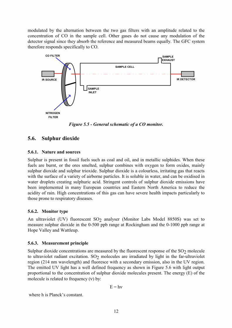
Radiation from an infrared (IR) source is passed through rotating gas filters containing CO in one and N2 in the other (see Figure 5.5). The CO gas filter acts to produce a reference beam which cannot be further attenuated by any CO that may be present in the sample cell. The N2 side of the filter wheel is transparent to the IR radiation and therefore produces a measured beam which can be absorbed by any CO present in the cell. The chopped detector signal is

(a + b)NO

aNO + bNO2

MOLYBDENUMCONVERTER

aNO + bNO2

OZONEGENERATOR

EXCESS OZONE

PHOTOMULTIPLIERTUBE

AMBIENTAIR SAMPLEINLET

VACUUMPUMP

REACTIONCHAMBER

Figure 5.4 - General schematic of a NOx monitor.

12

modulated by the alternation between the two gas filters with an amplitude related to the concentration of CO in the sample cell. Other gases do not cause any modulation of the detector signal since they absorb the reference and measured beams equally. The GFC system therefore responds specifically to CO.

5.6. Sulphur dioxide


Sulphur is present in fossil fuels such as coal and oil, and in metallic sulphides. When these fuels are burnt, or the ores smelted, sulphur combines with oxygen to form oxides, mainly sulphur dioxide and sulphur trioxide. Sulphur dioxide is a colourless, irritating gas that reacts with the surface of a variety of airborne particles. It is soluble in water, and can be oxidised in water droplets creating sulphuric acid. Stringent controls of sulphur dioxide emissions have been implemented in many European countries and Eastern North America to reduce the acidity of rain. High concentrations of this gas can have severe health impacts particularly to those prone to respiratory diseases.

5.6.2. Monitor type

An ultraviolet (UV) fluorescent SO2 analyser (Monitor Labs Model 8850S) was set to measure sulphur dioxide in the 0-500 ppb range at Rockingham and the 0-1000 ppb range at Hope Valley and Wattleup.


Sulphur dioxide concentrations are measured by the fluorescent response of the SO2 molecule to ultraviolet radiant excitation. SO2 molecules are irradiated by light in the far-ultraviolet region (214 nm wavelength) and fluoresce with a secondary emission, also in the UV region. The emitted UV light has a well defined frequency as shown in Figure 5.6 with light output proportional to the concentration of sulphur dioxide molecules present. The energy (E) of the molecule is related to frequency (ν) by:

E = hν

where h is Planck’s constant.

IR SOURCE

CO FILTER

NITROGENFILTER

IR DETECTOR

SAMPLEEXHAUST

SAMPLEINLET

SAMPLE CELL

Figure 5.5 - General schematic of a CO monitor.

13

5.7. Particulates


Particulates comprise small solid matter such as dust and smoke ranging from 10-9m to 10-4m in diameter. Inhaled particles with diameters less than 10µm (10x10-6m) can remain in the lungs and may cause health problems. Damage may result due to infection or to the toxicity of the particles themselves. Smaller particles, i.e. those less than 2.5µm (2.5x10-6m) in diameter, may lodge in the alveolar tissue of the lung where absorption into the blood must occur for removal. Inert particles may therefore remain trapped in the alveoli, decreasing the efficiency of respiration at that site.

5.7.2. Monitor type

(1) Visibility

An Integrating Nephelometer (Belfort Instrument Company Model 1591) set to measure the Scattering Coefficient in the 0 to 10x10-4m-1 range was used. (Refer to Figure 5.7).

SO2**

SO2*

SO2SO2

EnergyofMolecule UV Light absorption

heat liberated

light emitted

Figure 5.6 - Energy diagram of an excited SO2 molecule.

Figure 5.7 - Nephelometer mounting.

Figure 5.8 - TEOM on a metal base.

14

(2) Suspended particulates (integrating), TSP and PM10)

A High Volume Air Sampler (Cairns Instrument Services Mk 3) with either a Total Suspended Particulates (TSP) or a 10µm diameter or less (PM10) size selective head was used. (See Figures 5.9 and 5.10 respectively).

(3) Suspended particulates (continuous), PM2.5)

A Tapered Element Oscillating Microbalance (TEOM) ambient particulate monitor (Rupprecht & Patashnick Co., Inc. Model 1400a as shown in Figure 5.11) with a 2.5µm size selective head was used to measure particles less than 2.5µm in diameter. The monitor was set to measure in the range 0 to 400µg/m3.


(1) Visibility

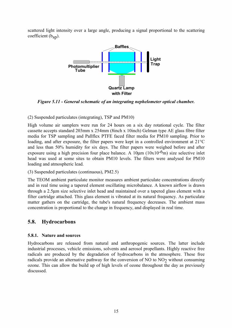
The Integrating Nephelometer measures the light scattering characteristics of the air. The ambient air sample is continuously drawn through an optical chamber illuminated by a diffuse light source with an effective wavelength centered on 530 nm. Figure 5.7 shows the arrangement of the light source and photomultiplier tube so that only scattered light is seen by the photomultiplier tube. The light received at the photomultiplier tube is therefore proportional to the total light scattered in all directions. The nephelometer integrates the

Figure 5.9 - High volume sampler with a TSP head.

Figure 5.10 - High volume sampler with PM10 head.

15

scattered light intensity over a large angle, producing a signal proportional to the scattering coefficient (bsp).

(2) Suspended particulates (integrating), TSP and PM10)

High volume air samplers were run for 24 hours on a six day rotational cycle. The filter cassette accepts standard 203mm x 254mm (8inch x 10inch) Gelman type AE glass fibre filter media for TSP sampling and Pallflex PTFE faced filter media for PM10 sampling. Prior to loading, and after exposure, the filter papers were kept in a controlled environment at 21°C and less than 50% humidity for six days. The filter papers were weighed before and after exposure using a high precision four place balance. A 10µm (10x10-6m) size selective inlet head was used at some sites to obtain PM10 levels. The filters were analysed for PM10 loading and atmospheric lead.

(3) Suspended particulates (continuous), PM2.5)

The TEOM ambient particulate monitor measures ambient particulate concentrations directly and in real time using a tapered element oscillating microbalance. A known airflow is drawn through a 2.5µm size selective inlet head and maintained over a tapered glass element with a filter cartridge attached. This glass element is vibrated at its natural frequency. As particulate matter gathers on the cartridge, the tube's natural frequency decreases. The ambient mass concentration is proportional to the change in frequency, and displayed in real time.

5.8. Hydrocarbons


Hydrocarbons are released from natural and anthropogenic sources. The latter include industrial processes, vehicle emissions, solvents and aerosol propellants. Highly reactive free radicals are produced by the degradation of hydrocarbons in the atmosphere. These free radicals provide an alternative pathway for the conversion of NO to NO2 without consuming ozone. This can allow the build up of high levels of ozone throughout the day as previously discussed.

LightTrap

Quartz Lampwith Filter

PhotomultiplierTube

Baffles

Figure 5.11 - General schematic of an integrating nephelometer optical chamber.

16

5.8.2. Monitor type

A Flame ionization THC-CH4-NMHC analyser (Horiba Model APHA-350E) is used and set to measure total hydrocarbon, methane and non-methane hydrocarbons in the range 0-10 ppmC.


The principle used to detect hydrocarbons is flame ionization detection (FID). There are two gas streams. The first stream passes directly into the detector for analysis. The second passes through a cutter, which burns heavier hydrocarbons leaving only methane. An electrode produces current proportional to the hydrocarbon concentration in both streams and hence provides the total hydrocarbon (THC) and CH4 levels. The difference between the two signals therefore becomes the non methane hydrocarbon (NMHC) level.

5.9. Photochemical Smog Two Airtrak 2000 instruments were purchased for the study and installed at Caversham and Swanbourne respectively. These instruments were designed by the CSIRO to measure the constituents of photochemical smog and to measure the photochemical reactivity of air, i.e. the rate at which smog is formed in the air under the influence of sunlight and temperature. Given this information it is possible to predict how much smog will be present in the air later in the day, or altenatively, determine the likely source of emissions reaching the Airtrak location.

Unfortunately the Airtrak instruments did not operate reliably for any useful length of time throughout the study due to a range of technical problems. It may be possible with further effort to extract some useful results. If this occurs, a technical report describing the instrument and its operation during the study will be prepared.

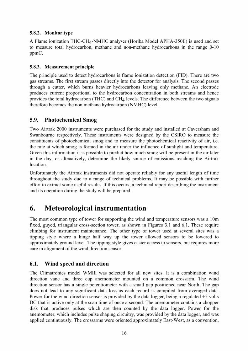
6. Meteorological instrumentation The most common type of tower for supporting the wind and temperature sensors was a 10m fixed, guyed, triangular cross-section tower, as shown in Figures 3.1 and 6.1. These require climbing for instrument maintenance. The other type of tower used at several sites was a tipping style where a hinge half way up the tower allowed sensors to be lowered to approximately ground level. The tipping style gives easier access to sensors, but requires more care in alignment of the wind direction sensor.

6.1. Wind speed and direction The Climatronics model WMIII was selected for all new sites. It is a combination wind direction vane and three cup anemometer mounted on a common crossarm. The wind direction sensor has a single potentiometer with a small gap positioned near North. The gap does not lead to any significant data loss as each record is compiled from averaged data. Power for the wind direction sensor is provided by the data logger, being a regulated +5 volts DC that is active only at the scan time of once a second. The anemometer contains a chopper disk that produces pulses which are then counted by the data logger. Power for the anemometer, which includes pulse shaping circuitry, was provided by the data logger, and was applied continuously. The crossarms were oriented approximately East-West, as a convention,

17

with the anemometer at the western end (refer Figure 6.1). This placed the wind direction potentiometer gap in the less important northerly sector. The standard height for measurement was 10m.

6.2. Air temperature The sensor selected for use at the new sites was a shielded but unaspirated thermistor made by Unidata. The thermistor, which has a logarithmic negative temperature coefficient, was connected in series with an accurate reference resistor. The regulated voltage from the data logger was applied across the resistor plus thermistor in series, with the voltage across the thermistor being the signal which was logged. The standard height for measurement was approximately 10m, being slightly below the anemometer.

6.3. Temperature lapse rate The differential air temperature near the ground, delta T, was measured at Caversham and Hope Valley using a linked pair of AD590 transducers manufactured in house. The sensors were positioned on the tower at six and 18 metres, and like the 10 metre air temperature measurements, were radiation shielded but not aspirated.

6.4. Relative humidity A Rotronics MP100F sensor was used for measurement of relative humidity. This is a capacitive style sensor, with high performance characteristics of low short-term drift and high long-term stability.

6.5. Radiation Solar and net radiation were measured at Caversham and Hope Valley. The sensors were placed in the northern sector of the fenced compound at a height of 1.5 metres. This placement minimised the amount of light lost due to shadows.

Global, or total solar radiation, was measured using an Eppley 7-48 black and white pyranometer. The millivolt level signal from the sensor was amplified to a 0-5 volt range for logging.

Net radiation was measured using a Middleton CN1 pyrradiometer. This sensor employs soft polythene domes which are kept inflated using bottled dry nitrogen. The sensor generated signal is bipolar, being negative for net outward radiation. The signal was translated and amplified to a monopolar 0-5 volt range.

Ultraviolet solar radiation was measured using an Eppley TUVR sensor, which measures in the range 295-385 nanometres. Amplification was similar to the global radiation signal.

Figure 6.1 - Meteorological equipment on a 10 metre guyed tower.

18

6.6. Air pressure A Vaisala model PTA427 barometric pressure transmitter was used at the Cullacabardee station, mounted on an inside wall of the monitoring shed. The interior mounting of the sensor did not cause any discernible errors in signal.

6.7. Rainfall Tipping bucket rain gauges made by Rimco were installed at Caversham and Kenwick in addition to the gauges existing at Hope Valley and Wattleup. These gauges have buckets which hold the equivalent of either 0.1 mm or 0.2 mm of rain before tipping. The tip event is noted by the data logger as a pulse and totalled during the data record period of 10 minutes.

7. Upper air profiling instrumentation Meteorological parameters of the upper air were sampled using three remote sensing instruments: a RASS (Radio Acoustic Sounding System) radar, two SODARS (Sound Detection and Ranging), and also a program of radiosonde releases.

7.1. Remote sensing The RASS radar and one of the SODARS were installed at Cullacabardee, a mid coastal plain location, with the other SODAR being sited initially on the escarpment at Gidgegannup, and later relocated to Rottnest Island. The two instruments at Cullacabardee were to some degree complementary in their height-range capabilities.

The operating characteristics of the RASS radar and two Sodars are summarised below. The quoted “Highest Level” reached by the instruments are manufacturer specifications which may not be achieved in each situation.

Characteristic Sodar winds

Cullacabardee Sodar winds Gidgegannup

Radar winds Cullacabardee

RASS temps Cullacabardee

Averaging time (mins) 30 30 30 30 Lowest level (m) 30 30 110 120 Highest level (m) 870 620 25001

42002 1500

Level resolution (m) 30 30 601 1052

60

NOTES : 1 - Operating in high resolution mode. 2 - Operating in low resolution mode.

7.1.1. RASS radar

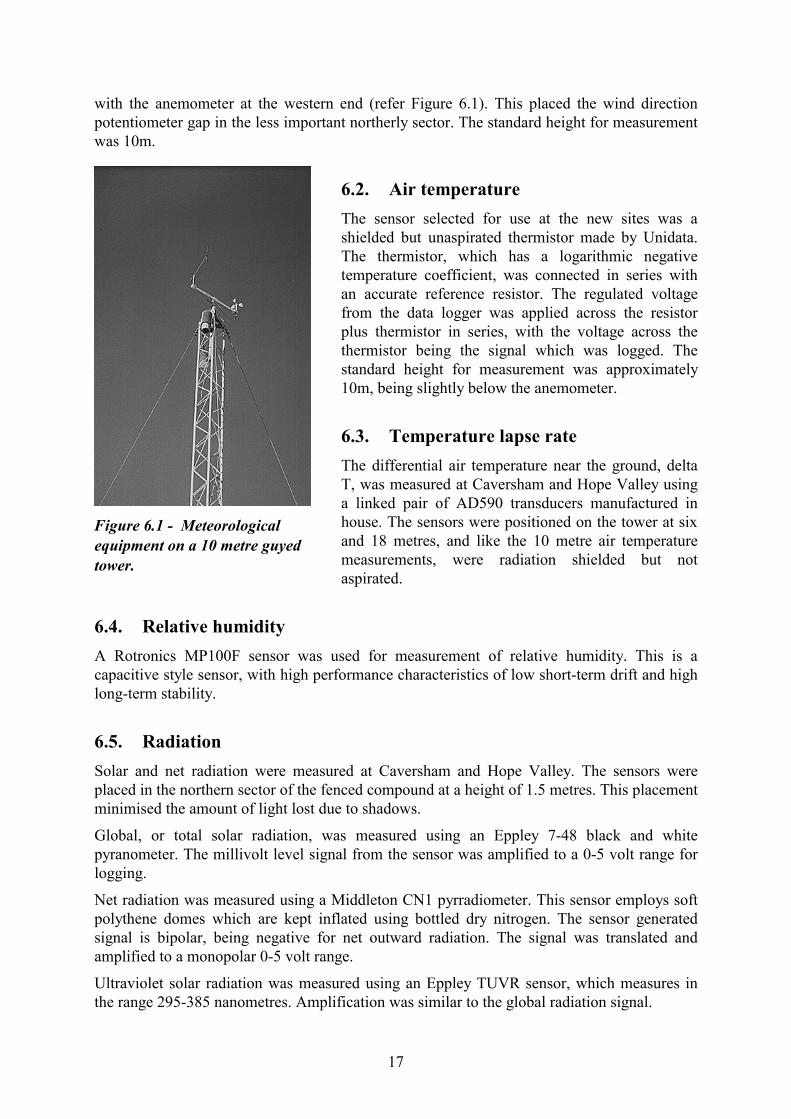
The RASS radar was used to determine the wind and temperature profile of the lower atmosphere. It uses a combination of techniques. Firstly a doppler radar of 915 MHz determines wind profiles up to approximately 4 km altitude. Secondly, an acoustic noise signal in combination with the electromagnetic radar is used to determine a temperature profile up to approximately 1.5 km. The RASS radar, a Radian LAP3000 model, is pictured in Figure 7.1 at the site of Cullacabardee. The central feature is the electromagnetic antenna which can configure itself electronically to point in one of three different directions; vertical,

19

plus two directions 15 degrees off vertical having horizontal directions that subtend a right angle. The ability of the antenna to act in three directions is achieved with the antenna maintaining a fixed physical position, using electronic phasing of the signal to simulate an angled antenna. The surrounding four enclosures are concrete pipes housing the acoustic loudspeakers. The speakers are directed downwards to an upwards facing parabolic dish. The acoustic signal is a continuous sounding band of frequencies centred around approximately 2KHz at a level of approximately 80 dB at close range. The site was chosen to be representative of the coastal plain, and is remote from nearby residences due to noise considerations.

The principles of operation are as follows. For wind profile measurement, the electromagnetic antenna operates in its three component mode to measure radial velocities in the three directions by the doppler shift method. Horizontal and vertical velocities at altitudes of interest are then calculated by resolving the vector velocities of the measured signals.

To measure the temperature profile, the electromagnetic radar goes into a vertical beam only mode, and the acoustic speakers are switched on to provide a continuous sound. The acoustic signal provides perturbations in the atmosphere travelling at a speed of sound governed by the temperature at each height. The radar measures the speed of sound at that height using the doppler shift technique, specifically utilising the strongest part of the return signal which occurs at the Bragg frequency, defined by the condition where the wavelength of the acoustic signal is exactly half of the radio signal wavelength. The speed of sound is calculated using the Bragg frequency part of the signal as other frequencies yield inaccurate values. The acoustic frequencies are spread over a band wide enough to include the Bragg frequency for all temperatures likely to be encountered. Calculating the speed of sound at each level then leads to the derivation of a corresponding virtual temperature.

Figure 7.1 - Radian LAP3000 model RASS located at Cullacabardee.

20

7.1.2. SODARS

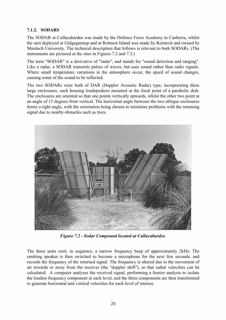
The SODAR at Cullacabardee was made by the Defence Force Academy in Canberra, whilst the unit deployed at Gidgegannup and at Rottnest Island was made by Remtech and owned by Murdoch University. The technical description that follows is relevant to both SODARs. (The instruments are pictured at the sites in Figures 7.2 and 7.3.)

The term "SODAR" is a derivative of "radar", and stands for "sound detection and ranging". Like a radar, a SODAR transmits pulses of waves, but uses sound rather than radio signals. Where small temperature variations in the atmosphere occur, the speed of sound changes, causing some of the sound to be reflected.

The two SODARs were both of DAR (Doppler Acoustic Radar) type, incorporating three large enclosures, each housing loudspeakers mounted at the focal point of a parabolic dish. The enclosures are oriented so that one points vertically upwards, whilst the other two point at an angle of 15 degrees from vertical. The horizontal angle between the two oblique enclosures forms a right angle, with the orientation being chosen to minimise problems with the returning signal due to nearby obstacles such as trees.

The three units emit, in sequence, a narrow frequency beep of approximately 2kHz. The emitting speaker is then switched to become a microphone for the next few seconds, and records the frequency of the returned signal. The frequency is altered due to the movement of air towards or away from the receiver (the "doppler shift"), so that radial velocities can be calculated. A computer analyses the received signal, performing a fourier analysis to isolate the loudest frequency component at each level, and the three components are then transformed to generate horizontal and vertical velocities for each level of interest.

Figure 7.2 - Sodar Compound located at Cullacabardee.

21

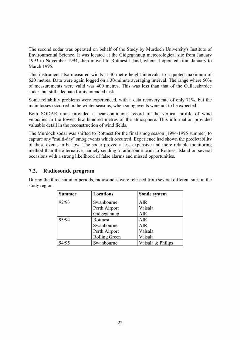
The Cullacabardee sodar operated from September 1992 onwards. It measured 30-minute average winds at 30 metre height intervals, with a quoted maximum range of 900 metres. In practice, 500 metres proved to be the effective upper limit for reliable data - considered to be good performance. The data recovery rate was fairly good through 1993, at over 85%, and better in 1994, at about 95%.

Data were initially recorded on a 10-minute averaging interval. This period was chosen for compatibility with the rest of the DEP's data logging, but was extended to 30 minutes on 18th February 1993, in the interests of improving the range of the instrument. The benefit of the change was seen as an increase in range by 50-100 metres (See Figure 7.4).

0

20

40

60

80

100

0 100 200 300 400 500 600HEIGHT (M)

Percent Frequencyof Maximum Range

30-minute averages

10-minute averages

Figure 7.4 - Frequency of valid wind velocity measurements made by the Cullacabardee sodar, for both 10 minute and 30 minute averaging intervals.

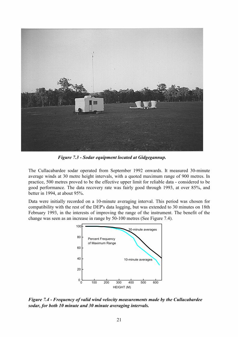
Figure 7.3 - Sodar equipment located at Gidgegannup.

22

The second sodar was operated on behalf of the Study by Murdoch University's Institute of Environmental Science. It was located at the Gidgegannup meteorological site from January 1993 to November 1994, then moved to Rottnest Island, where it operated from January to March 1995.

This instrument also measured winds at 30-metre height intervals, to a quoted maximum of 620 metres. Data were again logged on a 30-minute averaging interval. The range where 50% of measurements were valid was 400 metres. This was less than that of the Cullacabardee sodar, but still adequate for its intended task.

Some reliability problems were experienced, with a data recovery rate of only 71%, but the main losses occurred in the winter seasons, when smog events were not to be expected.

Both SODAR units provided a near-continuous record of the vertical profile of wind velocities in the lowest few hundred metres of the atmosphere. This information provided valuable detail in the reconstruction of wind fields.

The Murdoch sodar was shifted to Rottnest for the final smog season (1994-1995 summer) to capture any "multi-day" smog events which occurred. Experience had shown the predictability of these events to be low. The sodar proved a less expensive and more reliable monitoring method than the alternative, namely sending a radiosonde team to Rottnest Island on several occasions with a strong likelihood of false alarms and missed opportunities.

7.2. Radiosonde program During the three summer periods, radiosondes were released from several different sites in the study region.

Summer Locations Sonde system

92/93 Swanbourne Perth Airport Gidgegannup

AIR Vaisala AIR

93/94 Rottnest Swanbourne Perth Airport Rolling Green

AIR AIR Vaisala Vaisala

94/95 Swanbourne Vaisala & Philips

23

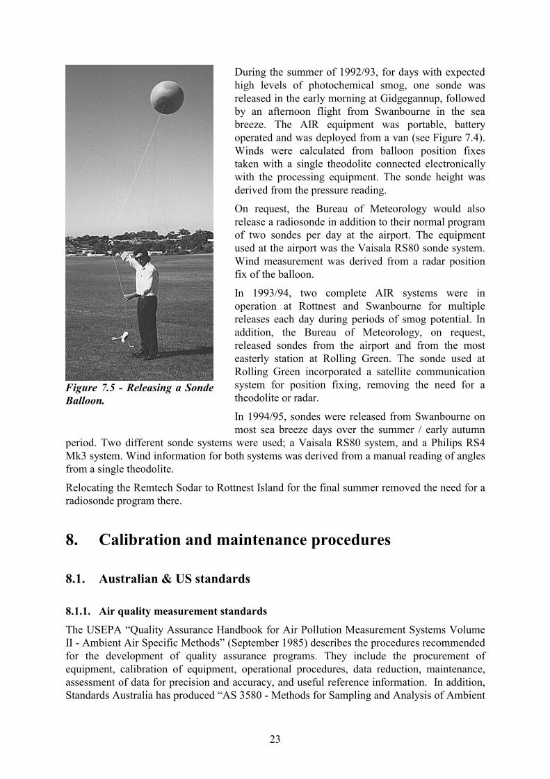
During the summer of 1992/93, for days with expected high levels of photochemical smog, one sonde was released in the early morning at Gidgegannup, followed by an afternoon flight from Swanbourne in the sea breeze. The AIR equipment was portable, battery operated and was deployed from a van (see Figure 7.4). Winds were calculated from balloon position fixes taken with a single theodolite connected electronically with the processing equipment. The sonde height was derived from the pressure reading.

On request, the Bureau of Meteorology would also release a radiosonde in addition to their normal program of two sondes per day at the airport. The equipment used at the airport was the Vaisala RS80 sonde system. Wind measurement was derived from a radar position fix of the balloon.

In 1993/94, two complete AIR systems were in operation at Rottnest and Swanbourne for multiple releases each day during periods of smog potential. In addition, the Bureau of Meteorology, on request, released sondes from the airport and from the most easterly station at Rolling Green. The sonde used at Rolling Green incorporated a satellite communication system for position fixing, removing the need for a theodolite or radar.

In 1994/95, sondes were released from Swanbourne on most sea breeze days over the summer / early autumn

period. Two different sonde systems were used; a Vaisala RS80 system, and a Philips RS4 Mk3 system. Wind information for both systems was derived from a manual reading of angles from a single theodolite.

Relocating the Remtech Sodar to Rottnest Island for the final summer removed the need for a radiosonde program there.

8. Calibration and maintenance procedures

8.1. Australian & US standards

8.1.1. Air quality measurement standards

The USEPA “Quality Assurance Handbook for Air Pollution Measurement Systems Volume II - Ambient Air Specific Methods” (September 1985) describes the procedures recommended for the development of quality assurance programs. They include the procurement of equipment, calibration of equipment, operational procedures, data reduction, maintenance, assessment of data for precision and accuracy, and useful reference information. In addition, Standards Australia has produced “AS 3580 - Methods for Sampling and Analysis of Ambient

Figure 7.5 - Releasing a Sonde Balloon.

24

Air”. Each method discusses the measurement principle, apparatus, sampling requirements, and operational procedures for each type of air quality monitoring equipment.

8.1.2. Meteorological measurement standards

The “USEPA Measurement Systems: Volume IV - Meteorological Measurements (revised August 1989)” describes the recommendations for standards of meteorological sensors used in pollution studies. Recommendations for wind instruments are well covered in Australian Standard AS2923. Regular maintenance and calibration of sensors, described later, led to accuracies that satisfy the documents quoted.

8.2. Calibration procedures

8.2.1. Air quality monitor calibration procedures

The O3, NOx, CO, HC, and SO2 analysers were calibrated using three span points and a zero once a month during non-summer months, with the SO2 monitor also receiving a mid-month calibration. During summer, all monitors were calibrated twice monthly. Integrating nephelometers were calibrated with one span point and a zero twice monthly throughout the year .

Calibrations for all gas monitoring equipment were performed on-site using certified span gases and calibrated gas blending equipment (GBE). Calibration of GBE was performed at the central workshop facility. The Unit Instruments UCS-200 GBE span channel was calibrated every three months at 90%, 70%, 50% and 30% of its full scale output while the Ecotech 8370 GBE span channel was calibrated at 75%, 50% and 25% of its full scale output.

All diluent gas flows were converted to their correct standard temperature (0°C) and pressure (1013.25 hPa) (STP) flow values by multiplying the measured flow by a Flow Correction Factor (FCF) calculated on site.

Pa-PH20-Palt 273.15(K) FCF = ------------- x -------- 1013.25(hPa) Ta(K)

• Pa ambient pressure at sea level • Ta ambient temperature • PH2O saturated water vapour pressure @ Ta • Palt altitude correction factor

The span gas flows used in all gas monitor calibrations were those determined at the three monthly GBE calibrations and were assumed to remain constant throughout the three month period between calibrations. The flow at each selected span point was calculated to reflect its value at STP.

The calibration formula was determined using the method of least squares. If the calculated correlation coefficient squared (r2) was less than 0.9998, the slopes of each individual span point and the zero point was calculated. Any point that showed a significant deviation from the median value of all the individual slopes was re-done.

8.2.2. Meteorological measurement calibration procedures

Compared to air quality instrumentation, the sensitivities of meteorological instrumentation are inherently more stable, allowing for a less intense program of calibrations.

25

Wind direction sensors were calibrated every six months. A measurement of the orientation of the crossarm formed the first part of the calibration, the method depending on the type of tower in use. Fixed towers, which have wind sensors installed with the crossarm pointing at a landmark were checked to see that there had not been any displacement. Any displacement was measured by a theodolite. The crossarm alignment measurement for other types of tower was performed by aligning a theodolite with the crossarm and taking a sunshot. Both methods were checked using a compass. The second part of the calibration used a custom made clamp to hold the wind vane parallel to the crossarm thereby producing a two point calibration to convert the logged voltage to an angle.

The calibration of wind sensors was performed using methods which removed the need to wind tunnel test every sensor on a regular basis. Initially, two of the anemometers were wind tunnel tested by the manufacturer to confirm the applicability of the standard calibration provided with the particular model of anemometer. One of these anemometers was further tested in the CSIRO wind tunnel in Melbourne. Confidence in the standard calibration was maintained by data checking procedures and by replacing the bearings. The data checking procedures for anemometers included inter-station comparisons and also identification of problems such as increases in the stall speed. Cups were checked during every visual inspection for any deterioration of surfaces which might affect aerodynamics. When data from an anemometer were suspect calibrations were checked by comparison with a co-located anemometer.

Air temperature sensors were checked every six months using a psychrometer, the thermometers of which had been calibrated by the Bureau of Meteorology in Melbourne. Any discrepancies were incorporated in the instrument calibration file rather than an adjustment of the sensor electronics.

Temperature difference, or delta T, was calibrated once a year using a dual water bath technique for the two sensors. One bath would be gradually heated to provide a temperature difference. The sensors were exchanged to provide a temperature difference of opposite polarity.

Relative humidity sensors were calibrated every six months using a small enclosing chamber with a standard salt solution enclosed. The electronics were adjusted to align with the two levels of 35% and 80% humidity.

Radiation sensors were calibrated annually by the Bureau of Meteorology in Melbourne. The DC amplifier which boosted each radiometer signal up to a level preferred by the logger was calibrated every six months.

Rain gauges were calibrated once each year by dripping a known amount (one litre) of water into the gauge. An over sampling indicated a need to clean the bucket.

8.3. Preventative maintenance Preventative maintenance is an orderly program of positive actions taken to minimise the failure of equipment. Good preventative maintenance will increase the amount of time the equipment is operational. When equipment is operating well, it also leads to improved quality. Both air quality instrumentation and meteorology equipment were subject to preventative maintenance programs.

26

8.3.1. Air quality monitoring equipment

A weekly service check was conducted at all monitoring locations to check those items the daily telemetry data was not capable of including. This included the state of the sample filters, level of compressed gas supplies, chart recorder paper and ink, and various monitor diagnostic test procedures.

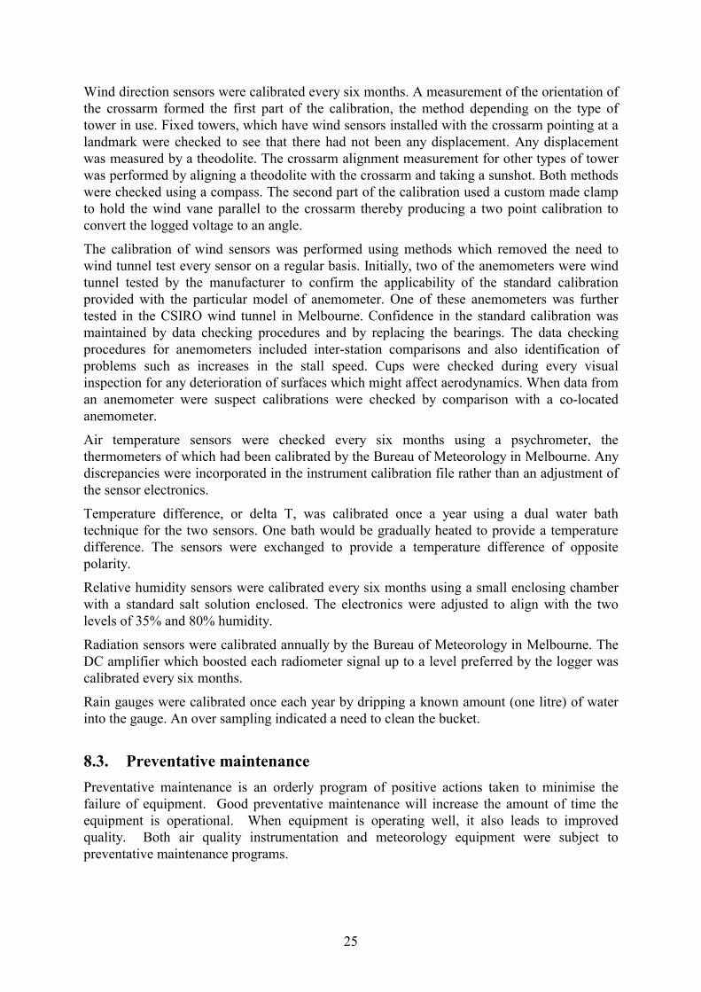
A schedule of preventative maintenance was drawn up for each item of air quality monitoring equipment, which is summarised in Table 8.1.

8.3.2. Meteorological equipment

The maintenance of instrument performance was achieved in a program containing three main elements. The related matter of instrument calibration is covered in Section 8.2.2. Data quality was checked daily (weekdays only) at the central computing facility in head office by inspecting the data retrieved by telemetry. This practice allows for comparisons between stations to easily identify instrument problems at one of the stations.

Field sites were visited between one and four times per month depending on the site instrumentation. A visual check of meteorological sensors can reveal an instrument problem that may not readily show up in a data inspection. Potential problems may also be averted by timely visual checks of instruments. Examples of these types of problems would be where deterioration may be gradual in nature such as the shading of a radiation sensor due to a fast growing bush or the gradual bending of a wind vane due to a perching bird.

The third element was a routine program of cleaning and parts replacement specific to each instrument. For some instruments, such as radiation sensors, this cleaning would occur with every visit. The polythene domes of net radiometers were replaced as necessary, several times per year. Rain gauges were cleaned once each year. Wind sensors were exchanged annually with a spare instrument, allowing for a general service of bearings and other components.

TABLE 8.1 : Air quality monitor preventative maintenance schedule.

MONITOR MAINTENANCE GOALS MONTHLY 3 6 12 Ozone/CO Clean optical bench � Recalibrate p&t transducers � Test d/a converter � Clean chassis, fan filter � Clean pneumatic system � NOX Check and clean capillaries � Inspect and/or clean cooler fins � Check NO2 to NO converter � SO2 Inspect chopper assembly � Replace charcoal scrubber � Clean pneumatic system � Clean exhaust orifice & filter � Inspect/replace uv lamp � Replace zero/span filter � Replace chopper belt � Rebuild vacuum pump � Nephelometer Clean optical assembly � Hydrocarbon Replace sample pump diaphragm � Replace suction pump diaphragm �

27

Some coastal sites received more frequent servicing due to the corrosive nature of the marine atmosphere. Radiation shields of temperature sensors were cleaned of dust as required, especially during summer when rain was infrequent.

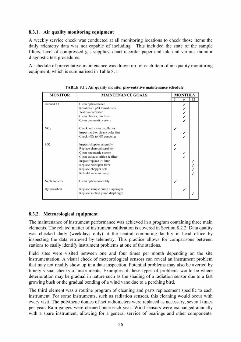
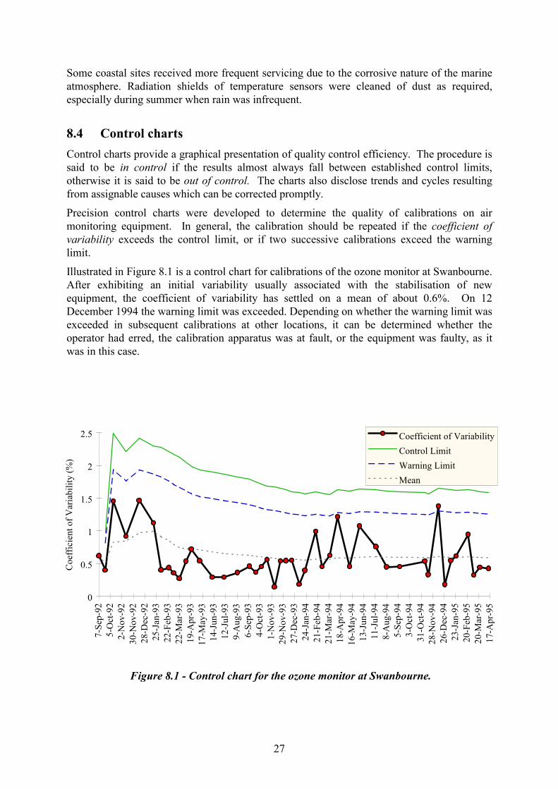
8.4 Control charts Control charts provide a graphical presentation of quality control efficiency. The procedure is said to be in control if the results almost always fall between established control limits, otherwise it is said to be out of control. The charts also disclose trends and cycles resulting from assignable causes which can be corrected promptly.

Precision control charts were developed to determine the quality of calibrations on air monitoring equipment. In general, the calibration should be repeated if the coefficient of variability exceeds the control limit, or if two successive calibrations exceed the warning limit.

Illustrated in Figure 8.1 is a control chart for calibrations of the ozone monitor at Swanbourne. After exhibiting an initial variability usually associated with the stabilisation of new equipment, the coefficient of variability has settled on a mean of about 0.6%. On 12 December 1994 the warning limit was exceeded. Depending on whether the warning limit was exceeded in subsequent calibrations at other locations, it can be determined whether the operator had erred, the calibration apparatus was at fault, or the equipment was faulty, as it was in this case.

0

0.5

1

1.5

2

2.5

7-Se

p-92

5-O

ct-9

22-

Nov

-92

30-N

ov-9

228

-Dec

-92

25-J

an-9

322

-Feb

-93

22-M

ar-9

319

-Apr

-93

17-M

ay-9

314

-Jun

-93

12-J

ul-9

39-

Aug

-93

6-Se

p-93

4-O

ct-9

31-

Nov

-93

29-N

ov-9

327

-Dec

-93

24-J

an-9

421

-Feb

-94

21-M

ar-9

418

-Apr

-94

16-M

ay-9

413

-Jun

-94

11-J

ul-9

48-

Aug

-94

5-Se

p-94

3-O

ct-9

431

-Oct

-94

28-N

ov-9

426

-Dec

-94

23-J

an-9

520

-Feb

-95

20-M

ar-9

517

-Apr

-95

Coe

ffic

ient

of V

aria

bilit

y (%

)

Coefficient of VariabilityControl LimitWarning LimitMean

Figure 8.1 - Control chart for the ozone monitor at Swanbourne.

28

9. Data processing

9.1. Chemical data processing The 12 bit analogue-to-digital converter in each logger provides a resolution of 212 or 4096 levels from zero to the full scale output of each monitor. As the full scale output for most gas monitors is set at 0.50 Volts, the maximum resolution possible is therefore approximately 0.12mV (500mV/4096).

Data from each site was returned to the central computing facility in hexadecimal format and kept in a raw data file. Each line of raw data represents a 10 minute averaged output from all the monitors at a specific site. A sample of a raw data file is shown in Figure 9.1.

Figure 9.2 shows a site specific calibration file. This file lists the full scale output for each monitor, together with the location in the hex string of the byte numbers associated with each monitor's output. This is used to convert the raw data into voltages.

Software written by DEP staff and running on a Silicon Graphics Iris workstation calculated what fraction of the monitor's full scale output each byte represented, and then used this, together with the known full scale voltage output of the monitor, to determine the original output voltage. Using the most current calibration equation available for that piece of equipment, the voltage was converted to the relevant units and placed into the data base for that site.

Site: Kenwick A.Q.M.S. Logger Sampling time: 1.00 seconds Logging interval: 600 seconds Number of bytes per log: 27 The first record commences at 15:10:00 on the 04 07 1994 EC0E8B7A8FDF0056036302EF002601F2000400F60748038C031000 F30FF7401CFF003E03170230013F011A010400DE0716038C031C00 E40E4AF0C9DE004B03430213013501FA000400E00734038C032300

Figure 9.1 - Sample raw data file.

Site: Kenwick A.Q.M.S. First date for processing: 280892 Logging interval (seconds): 0600 Number of variables per log: 13 PARAMETER INFORMATION: param param chan zero full error min val byte numbers name units no. scale code (-9 = no min) xH xL yH yL WSPD10 m/s 1 0.000 2.55 -99.0 0.0 26 WDIR10 DEGS 2 0.000 5.00 -99.0 0.0 2 1 3 D SIGMA10 DEGS 3 0.000 5.00 -99.0 0.0 7 6 5 4 S ATEMP10 DEG C 4 0.000 5.00 -99.0 0.0 9 8 T O3 PPHM 5 0.000 0.50 -99.0 0.0 11 10 NO PPHM 6 0.000 0.50 -99.0 0.0 13 12 NO2 PPHM 7 0.000 0.50 -99.0 0.0 15 14 VISI Bsp 8 0.000 0.50 -99.0 0.0 17 16 Spare none 9 0.000 0.50 -99.0 0.0 19 18 VAN TEMP Deg C 10 0.000 5.00 -99.0 0.0 21 20 ATEMP01 Deg C 11 0.000 5.00 -99.0 0.0 23 22 T Soil T Deg C 12 0.000 5.00 -99.0 0.0 25 24 Rainfall mm 13 0.000 2.55 -99.0 0.0 27

Figure 9.2 - Sample calibration file.

29

Once a month, all the data that had entered each site's data base for the previous month were reprocessed to replace any unwanted or incorrect data with error codes. The data removed included erroneous values due to calibrations, power failures, monitor repairs, monitor baseline drifts, and other spurious occurrences that were not representative or incorrectly reflected the conditions prevailing at the time. The site log-book contains the dates and times of calibrations, monitor repairs, etc. performed by maintenance staff. Remaining problems, such as power failures and instrument failures, were found by checking a computer plot of the monitor's voltage output. As the logger stores 10 minute averaged data, it is sometimes quite difficult to differentiate real data from invalid data. A situation may arise, for example, where there is a power failure for, say, two or three minutes. The 10 minute averaged data recorded by the logger will then be a combination of seven or eight minutes of valid data, and two to three minutes of invalid data. On the plot of the monitor's voltage output this may look real, but a check of the monitor's chart recorder trace, which records the monitor's instantaneous voltage output, will show that the monitor's output reduced to zero volts. As each monitor runs with an elevated baseline (typically 5%), an output of zero volts indicates a power failure or monitor fault. It can therefore be seen which data need to be removed from the data base.

When reprocessing the data, any drift in the monitor's response during the period between any two calibrations is assumed to be linear. A linear interpolation is consequently performed over time, from one calibration equation to the next, and an individual calibration equation generated from the interpolation for every 10 minute average. The newly calculated 10 minute average value is then re-entered into the data base, overwriting the original interim value. This method varies from the USEPA method of keeping the initial calibration slope fixed for the total period between calibrations.

9.2. Meteorological data processing The initial stages of data processing as described above are equally valid for the data from meteorological equipment. Data processing for the two types of equipment is different to the extent that there is no need for secondary processing of meteorological data; the calibrations of meteorological equipment being inherently more stable.

Meteorological data in the database are edited monthly for errors that occur due to power failures, instrument problems, and occasional unexplained transient data which are clearly incorrect.

The calibration file used to convert hexadecimal data to relevant S.I. units also contains information about certain meteorological channels which act as flags to allow for specialised data conversion to take place. These can be seen on the far right of each line in Figure 9.2. The meaning of each flag is shown below in Table 9.1.

30

Table 9.1 - Flag definitions as used in calibration files.

Flag used in Calibration

File

Used For

Meaning

D Wind Direction

To cope with the voltage jump at the potentiometer gap at north, the logger averaging allows for averages up to 720 degrees. The D flag converts the value to less than 360 degrees.

S Sigma Theta Signifies the need to use the extra bytes of averaging involved in the calculation of standard deviation.

T Air Temperature

Sensors which use a thermistor have a logarithmic output and so need a special logarithmic conversion, compared to the standard linear regression.

9.3. Daily data validation Each morning, time series plots of all 10 minute averaged data for the previous seven days were examined to determine whether any faults or breakdowns had occurred. Plots generated by software running on the Silicon Graphics Iris workstation are displayed on an IBM compatible 486DX personal computer running X terminal emulation software. These plots can be either the raw voltage data or the data base values, and can be any of the listed parameters in Table 2.1. Any monitor irregularities such as baseline drift or any power cuts that occurred were recognised and attended to. Figure 9.3 shows an example of the type of plot available. A calibration spike can be seen at midday on the 8th, and a power failure for 30 minutes in the early hours of the morning of the 12th.

8/8 9/8 10/8 11/8 12/8 13/8 14/8 0

50

100

150

200

O3mVOLTS

0

50

100

150

200

NOmVOLTS

0

50

100

150

200

NO2mVOLTS

Swanbourne A.Q.M.S, 1994

Figure 9.3 - Sample plot showing an elevated baseline, calibration and power failure.

31

9.4. Data Storage and access

9.4.1. Description of the data bases

Monitoring data recorded by the DEP are stored in a data base in fixed 10 minute time intervals using a random accessed, packed binary format (Rye,1983). Data are stored as one or two eight-bit bytes giving resolutions of 1/256 or 1/65,536 respectively. When the data are read, a linear transformation is performed to convert the stored integer number to the required values, e.g.,

wind speed (ms-1) = 0.1 * (stored number), gives a range of 0 - 25.5 ms-1, and

wind direction (deg) = 1.420 * stored number, gives a range of 0 - 360 deg.

9.4.2. Accessing the data

Various FORTRAN routines have been developed to write to, and access information from, each data base. Information in any data base can be accessed in various ways depending on its intended use e.g.

• data may be output to a sequential ASCII file to allow easy transfer to other users;

• data may be plotted to screen or a hard copy produced (see example in Figure 9.4);

• data bases may be directly accessed by computer models;

• monthly and annual statistics of data may be generated (see the example in Figure 9.5).

In the course of accessing the data, the desired unit of measurement and averaging time can be stipulated within most applications.

9.4.3. Data report

Limited numbers of a data summary report (graphical representations) will be made available for loan from the DEP to interested groups. More detailed data will be made available from Western Power and the DEP subject to the possibility that a charge may be applied when data is to be used for commercial purposes.

32

00 06 12 18 24 0

3

6

9

12

1500 06 12 18 24

0

90

180

270

36000 06 12 18 24

0 2 4 6 81012 Quinns Rocks A.Q.M.S., 8-Jan-1993

Figure 9.4 - Sample data base plot.

33

AIR QUALITY MONITORING STATION DATA =================================== SITE: Quinns Rocks A.Q.M.S. OZONE CONTINUOUS MONITOR STATISTICS VALUES QUOTED ARE PARTS PER BILLION TIMES QUOTED ARE AT THE END TIME OF THE AVERAGING PERIOD JANUARY 1993 DATE 8 HOUR 4 HOUR 1 HOUR 10 MIN. 1 HOUR %AGE MAX (TIME) MAX (TIME) MAX (TIME) MAX (TIME) PERIODS > 80 DATA 1 1 93 15.2 0010 15.3 0030 15.8 0810 16.0 0720 100. 2 1 93 18.9 1630 20.1 1400 21.5 1140 23.0 1140 100. 3 1 93 26.4 1940 31.0 1550 37.8 1400 39.0 1310 100. 4 1 93 34.6 2030 40.6 1630 57.7 1340 60.0 1310 100. 5 1 93 41.0 2050 52.2 1700 68.5 1440 71.0 1410 100. 6 1 93 42.7 2020 50.8 1630 68.0 1350 75.0 1320 100. 7 1 93 55.9 2130 65.4 1800 72.8 1520 76.0 1440 100. 8 1 93 57.9 1600 73.3 1250 91.3 1140 97.0 1050 2 100. 9 1 93 35.5 1840 36.0 1440 39.8 1140 45.0 1050 100. 10 1 93 34.0 1640 38.8 1330 46.8 1250 49.0 1250 100. 11 1 93 29.7 1740 30.3 1440 33.2 1050 38.0 1000 100. 12 1 93 39.1 1730 47.5 1420 56.3 1250 67.0 1210 100. 13 1 93 25.2 1510 29.5 1300 34.8 1150 36.0 1120 100. 14 1 93 11.1 0010 12.5 1310 13.8 1130 14.0 1030 100. 15 1 93 16.4 2400 21.0 2350 21.7 2340 22.0 2310 100. 16 1 93 19.7 0300 21.0 0010 21.8 1100 23.0 1040 100. 17 1 93 27.5 1650 32.9 1400 36.7 1240 38.0 1240 100. 18 1 93 19.6 1630 24.0 1310 27.0 1110 28.0 1110 100. 19 1 93 14.9 2240 16.2 2110 17.7 1050 19.0 1030 100. 20 1 93 24.3 1900 27.2 1700 28.8 1410 30.0 1400 100. 21 1 93 28.5 1420 41.4 1420 60.3 1330 62.0 1300 95. 22 1 93 30.8 1510 41.7 1340 49.0 1210 51.0 1130 100. 23 1 93 14.5 1010 15.0 0910 15.0 0610 15.0 0520 100. 24 1 93 35.2 2030 43.0 1750 45.7 1600 47.0 1520 100. 25 1 93 28.9 1550 35.2 1340 40.5 1310 41.0 1240 100. 26 1 93 20.7 1830 21.6 1500 23.0 1150 24.0 1120 100. 27 1 93 33.2 1750 35.4 1400 40.5 1110 47.0 1100 100. 28 1 93 29.5 1640 35.7 1320 40.3 1230 43.0 1210 100. 29 1 93 36.8 1900 40.0 1530 46.8 1230 51.0 1220 100. 30 1 93 26.2 1620 32.2 1220 44.3 0940 52.0 0920 100. 31 1 93 28.5 1820 33.7 1500 36.2 1310 41.0 1240 100. MONTHLY AVERAGE: 18.1 MAXIMUM 8 HOUR AVERAGE: 57.9 MAXIMUM 4 HOUR AVERAGE: 73.3 MAXIMUM 1 HOUR AVERAGE: 91.3 MAXIMUM 10 MIN. AVERAGE: 97.0 8 HR PERIODS> 50: 2, 80: 0 4 HR PERIODS> 50: 6, 60: 2 1 HR PERIODS> 80: 2, 120: 0 10 MN PERIODS> 80: 6, 120: 0 DATA RECOVERY FOR MONTH: 99.8%

Figure 9.5 - Sample monthly report.

34

10. References Rye, P.J., 1983. “Digitising and Processing Anemometer Chart Data”, Western Australian Institute of Technology, School of Physics and Geosciences, Report No.SPG 324/1983/AP60, August 1983.

The Perth Photochemical Smog Study monitoring network · 2016-01-21 · The Perth Photochemical...

Documents

Transcript of The Perth Photochemical Smog Study monitoring network · 2016-01-21 · The Perth Photochemical...