The Performance of Drag Embedment Anchors (DEA)

by

Charles Aubeny, Texas A&M University

Robert Gilbert, The University of Texas at Austin

Robert Randall, Texas A&M University

Evan Zimmerman, Delmar

Katelyn McCarthy, The University of Texas at Austin

Ching-Hsiang Chen, The University of Texas at Austin

Aaron, Drake, Texas A&M University

Po Yeh, Texas A&M University

Chao-Ming Chi, Texas A&M University

Ryan Beemer, Texas A&M University

Final Project Report

Prepared for Minerals Management Service Under Contract Number M09PC00028

MMS Project Number 645 OTRC Project 32558-A6960

March 2011

OTRC Library Number: 12/10C201

For more information contact:

Offshore Technology Research Center Texas A&M University

1200 Mariner Drive College Station, Texas 77845-3400

(979) 845-6000

or

Offshore Technology Research Center The University of Texas at Austin

1 University Station C3700 Austin, Texas 78712-0318

(512) 471-6989

A National Science Foundation Graduated Engineering Research Center

“The views and conclusions contained in this document are those of the authors and should not be interpreted as representing the opinions or policies of Minerals Management Service. Mention of trade names or commercial products does not constitute their endorsement by Minerals Management Service.

i

TableofContentsTable of Contents ............................................................................................................................. i 

List of Tables ................................................................................................................................. iv 

List of Figures ................................................................................................................................. v 

Executive Summary ........................................................................................................................ x 

1.0  Introduction ......................................................................................................................... 1 

1.1  Objective .......................................................................................................................... 1 

1.2  Background ...................................................................................................................... 3 

1.3  Scope of Work .................................................................................................................. 4 

1.4  Structure of Report ........................................................................................................... 5 

2.0  Small (1:30) Scale Model Tests .......................................................................................... 7 

2.1  Introduction ...................................................................................................................... 7 

2.2  Experimental Equipment and Facility .............................................................................. 8 

2.2.1  Experiment Facility ................................................................................................... 8 

2.2.2  Kaolinite Clay ......................................................................................................... 11 

2.2.2.1  T-Bar ................................................................................................................... 13 

2.2.2.2  Thermo-Plastic Tank ........................................................................................... 14 

2.2.2.3  Metal Tank .......................................................................................................... 15 

2.2.3  Magnetometer for Tracking ........................................................................................... 16 

2.3  Small (1:30) Scale Model Anchor .................................................................................. 17 

2.4  Pure Loading Tests ......................................................................................................... 20 

2.4.1  Pure Translation Tests ............................................................................................. 20 

2.4.1.1  Procedure ............................................................................................................. 20 

2.4.1.2  Results ................................................................................................................. 22 

2.4.1.3  Analysis ............................................................................................................... 22 

2.4.2  Pure Rotation Tests ................................................................................................. 27 

2.5  Drag Tests ...................................................................................................................... 29 

2.5.1  In-plane drag embedment tests ............................................................................... 30 

2.5.2  Out-of-plane Drag Embedment Tests ..................................................................... 45 

3.0  Large-Scale Tests .............................................................................................................. 50 

ii

3.1  Introduction .................................................................................................................... 50 

3.2  Experimental Test Arrangements ................................................................................... 50 

3.2.1  Carriage and Tow Tank Test Arrangements ........................................................... 51 

3.2.2  Sediment Pit Layout and Global Coordinates ......................................................... 54 

3.2.3  Sediment (Mud) Mixing Device ............................................................................. 56 

3.2.4  Anchor and towline characteristics ......................................................................... 57 

3.3  Instrumentation and Data Collection .............................................................................. 59 

3.3.1  Pressure Transducer ................................................................................................ 60 

3.3.2  Anchor Force Transducer ....................................................................................... 61 

3.3.3  Anchor 2-Axis Inclination Sensor .......................................................................... 62 

3.3.4  Carriage and Breakout Force Transducer ............................................................... 62 

3.3.5  T-bar and Rotational Breakout Tests Force Transducers ....................................... 63 

3.3.6  Towline and Chaser Angle Position Sensors .......................................................... 63 

3.3.7  Chaser Line Displacement Sensor .......................................................................... 63 

3.3.8  Towline and Chaser Cable Apparatus ..................................................................... 64 

3.4  Sediment Strength Testing ............................................................................................. 65 

3.5  Breakout Devices and Procedures .................................................................................. 67 

3.5.1  Normal Breakout Test Apparatus and Procedures .................................................. 67 

3.5.2  Transverse Breakout Test Apparatus and Procedures ............................................ 67 

3.5.3  Rotational Breakout Test and Procedures ............................................................... 69 

3.6  In-plane Towing Test Procedures .................................................................................. 70 

3.7  Out-of-Plane Towing Test Procedures ........................................................................... 71 

3.7.1  Case 1. Initial Surface and Sub-surface Out-of-Plane ............................................ 71 

3.7.2  Case 2. Main Pull Line Out-of-Plane Tests ............................................................ 72 

3.7.3  Case 3. Carriage Ladder Mounted Out-of-Plane Tests .......................................... 75 

3.8  Dredge/Tow Carriage Operation .................................................................................... 76 

3.9  Results of Testing Drag Embedment Anchors ............................................................... 79 

3.9.1  In-Plane Results ...................................................................................................... 79 

3.9.2  Out-of-Plane Results ............................................................................................... 91 

3.9.3  Break-out Results ................................................................................................... 99 

iii

3.10  Summary and Conclusions ........................................................................................... 100 

4.0  Model Development and Evaluation .............................................................................. 103 

4.1  In-Plane Behavior ......................................................................................................... 103 

4.1.1  Load Capacity ....................................................................................................... 103 

4.1.2  Anchor Line Behavior ........................................................................................... 110 

4.1.3  Trajectory during Drag Embedment ..................................................................... 112 

4.1.4  Adjustments to In-Plane Behavior Model ............................................................. 116 

4.1.5  Comparison of 1:30 Scale Model Tests with Model ............................................ 119 

4.2  Out-of-Plane Trajectory Behavior ................................................................................ 138 

4.2.1  Theoretical Considerations ................................................................................... 138 

4.2.2  Experimental Data ................................................................................................ 145 

4.2.3  Example Out-of-Plane Behavior ........................................................................... 158 

5.0  Recommended Capacity Curves for Generic Anchor ..................................................... 164 

6.  Conclusions and Recommended Future Work ................................................................... 171 

References ................................................................................................................................... 178 

Appendix I. Large Scale Testing Project Data ............................................................................ 179 

Appendix II. Tests in Kaolinite Bed .......................................................................................... 183 

Appendix III: Engineering Interpretation of Large-Scale Test Data ......................................... 267 

Appendix IV: Delmar DEA Investigation ................................................................................. 291 

Appendix V – Tests in Laponite Test Bed .................................................................................. 328 

iv

ListofTablesTable 2.1. Physical properties for 1:30 model anchor ................................................................. 19 Table 2.2. Areas of different surfaces for 1:30 scale model anchor ............................................ 19 Table 2.3. Results and analysis of pure translation loading tests for 1:30 scale model .............. 22 Table 2.4. Summary of Theoretical and Experimental Bearing Capacity Factors for Pure Translational Loading ................................................................................................................... 24 Table 2.5. Table of Bearing Capacity Calculations: In-Plane Shear – Plugged, In-Plane Shear Unplugged, Normal and Out-of-Plane Shear ................................................................................ 25 Table 2.5a. In-Plane Shear ........................................................................................................... 25 Table 2.5b. Normal ...................................................................................................................... 26 Table 2.5c. Out-of-Plane Shear ..................................................................................................... 26 Table 2.6. Results and Analysis of Pure Rotational Loading Tests ............................................ 29 Table 2.7. Comparison of Ta and Ne ............................................................................................ 42 Table 2.8. Calculated Ne* Values for tests Performed ................................................................ 43 Table 2.9. Out of Plane Ne Values for Tests Performed .............................................................. 49 Table 3.1. Definitions and characteristics of generic model anchor and instrumentation. ......... 54 Table 3.2. Sediment pit sand, bentonite, and water percentages and bulk density. ..................... 56 Table 3.3. Case 2 out-of-plane pull distance. ............................................................................... 73 Table 3.4. Case 2 out-of-plane offset distances. ......................................................................... 75 Table 3.5. Performance of model drag embedment anchor in-plane test plan. ........................... 80 Table 3.6. Model drag embedment anchor out-of-plane test plan. .............................................. 92 Table 3.7. Model drag embedment anchor breakout test plan. .................................................... 99 Table 4.1. Significant Features of Large and Small Scale Laboratory Model Tests ................. 108 Table 4.2. Comparison of Large and Small Scale In-Plane Test Results .................................. 110 Table 4.3. Anchor Parameters used in Small-Scale Test Comparisons to Model ...................... 119 Table 4.4. Test bed Parameters used in Small-Scale Test Comparisons to Model .................... 123 

Table 4.5 Tilt v of Plane of Trajectory: Model Predictions versus Measurement ..................... 159 Table 5.1. Generic Anchor Holding Capacity Relations, Af/b

2 = 1500, 50-degree fluke-shank angle with Bearing Factor Ne=4 .................................................................................................. 166 Table 5.2. Generic Anchor Holding Capacity Relations, Af/b

2 = 1500, 50-degree fluke-shank angle with Bearing Factor Ne=5 .................................................................................................. 167 Table 5.3. Generic anchor holding capacity relations for wire anchor lines with 100-m drag distance, 50-degree fluke-shank angle with Ne=4 ....................................................................... 169 Table 5.4. Generic Anchor Holding Capacity Relations, Af/b

2 = 1500, 36-degree fluke-shank angle ............................................................................................................................................ 170 

v

ListofFiguresFigure 2.1. Loading frame ............................................................................................................. 8 Figure 2.2. Loading device ............................................................................................................ 9 Figure 2.3. Load cell ................................................................................................................... 10 Figure 2.4. Data acquisition and control system .......................................................................... 11 Figure 2.5. Water Content vs. Undrained Shear Strength (Lee 2008) .......................................... 12 Figure 2.6. T-Bar test .................................................................................................................... 13 Figure 2.7. Drill with steel paddle and mixing process in the thermoplastic tub ........................ 14 Figure 2.8. Thermo Plastic Tank on Elevated Platform ............................................................... 15 Figure 2.9 - Testing Facility.......................................................................................................... 16 Figure 2.10. Testing Facility for use of the Magnetometer .......................................................... 17 Figure 2.11. 1:30 Scale Model Anchor ......................................................................................... 18 Figure 2.12. Area 1 through 7 presented in Table 2.2 ................................................................. 19 Figure 2.13. Magnetometer attached to 1:30 scale model ........................................................... 20 Figure 2.14. In-plane Shear Test Orientation (Left: Just Anchor and Right: With Magnetometer Sensor) .......................................................................................................................................... 21 Figure 2.15. Out-of-plane Shear Orientation  Figure 2.16. Normal Orientation. ..................... 21 Figure 2.17. Test setup for pure rotational loading test ............................................................... 27 Figure 2.18. Attachment of the Anchor to the Threaded Rod for each Orientation .................... 28 Figure 2.19. Testing Tracks in Metal Tank .................................................................................. 30 Figure 2.20. Example Test Configuration for In-Plane Drag Embedment Test .......................... 31 Figure 2.21. Trajectory of an In-Plane Drag Embedment Tests .................................................. 32 Figure 2.22. Illustration of In-plane Drag test with Steep Anchor Line ...................................... 34 Figure 2.23. Illustration of In-plane Drag Test with Magnetometer ............................................ 35 Figure 2.24. Out-of-plane drag test data with the Magnetometer ................................................ 36 Figure 2.25. Effect of Initial Pitch Angle on Pitch and the Trajectory ....................................... 37 Figure 2.26. Line Displacement vs. Load cell readings and Interpolated Trajectory ................. 39 Figure 2.27. Example of Undrained Shear Strength Profile ........................................................ 41 Figure 2.28. Ne vs. Line Displacement and Embedment Depth ................................................. 44 Figure 2.29. Variation in dn/ds throughout Drag Distance .......................................................... 44 Figure 2.30. Trajectory for Out-of-plane Test ............................................................................. 47 Figure 2.28. Out-of-plane drag test data with the Magnetometer. ............................................... 48 Figure 3.1. Schematic of the Dredge/Tow Tank in the Haynes Coastal Engineering Laboratory at Texas A&M University. ................................................................................................................ 51 Figure 3.2. General test configuration with the main pull line (grey) and data acquisition chaser line (dashed). ................................................................................................................................. 52 Figure 3.3. Pull angle adjustments ............................................................................................... 52 Figure 3.4. Instrumentation used for drag embedment testing. ................................................... 53 Figure 3.5. Bracket detail. ............................................................................................................ 53 

vi

Figure 3.6. Sediment mixture operation outside and discharging sediment into sediment pit in the towing flume. .......................................................................................................................... 55 Figure 3.7. Sediment pit global coordinates and profile. ............................................................. 55 Figure 3.8. Support structure and sediment pit. ........................................................................... 56 Figure 3.9. Sediment mixing device. ........................................................................................... 57 Figure 3.10. S ediment surface after recent mixing. ..................................................................... 57 Figure 3.11. Anchor fluke angle settings. .................................................................................... 58 Figure 3.12. Anchor dimensions and centroid. ............................................................................ 59 Figure 3.13. Anchor instruments layout. ..................................................................................... 60 Figure 3.14. Pressure transducer mounted on bottom side of model anchor. .............................. 61 Figure 3.15. Anchor force transducer attached to shank of model anchor. ................................. 61 Figure 3.16. Anchor pitch and roll sign convention. ................................................................... 62 Figure 3.17. Chaser line displacement sensor. ............................................................................. 64 Figure 3.18. Towline pulley apparatus (right) and chaser cable apparatus. ................................ 65 Figure 3.19. Tow and chaser line angle convention. ................................................................... 65 Figure 3.20. T-bar sediment strength measurement device. ........................................................ 66 Figure 3.21. T-bar test locations. ................................................................................................. 67 Figure 3.22. Transverse breakout test apparatus. ......................................................................... 68 Figure 3.23. Model anchor rotational coordinates. ...................................................................... 69 Figure 3.24. Rotational breakout setup pictures. ......................................................................... 70 Figure 3.25. In-plane initial anchor placement. ........................................................................... 71 Figure 3.26. Case 1 surface out-of-plane. .................................................................................... 72 Figure 3.27. Example paths for 15° out-of-plane. ....................................................................... 74 

Figure 3.28. Pull paths for 30° and 45° out-of-plane. ................................................................. 74 

Figure 3.29. Ladder mounted out-of-plane pull path example ................................................... 76 Figure 3.30. Dredge/tow carriage and sediment pit (left) and model anchor being lifted out of the mud after a test (right). ............................................................................................................ 77 Figure 3.31. Dredge/tow carriage control console (left) and sediment pit with mud mixer (right)........................................................................................................................................................ 77 Figure 3.32. Manual control system (left) and PC control system and horizontal position laser mounted on the dredge/tow carriage (right). ................................................................................. 78 Figure 3.33. Computer screen for tow carriage operation during model drag embedment anchor testing. ........................................................................................................................................... 79 Figure 3.34. In-plane anchor measurements for test number 10. ................................................ 82 Figure 3.35. In-plane measurements for chaser, anchor, displacement, and pitch and roll for test 10................................................................................................................................................... 83 Figure 3.36. In-plane anchor measurements for test 13. .............................................................. 84 Figure 3.37. In-plane angle measurements for test 13. ................................................................ 85 Figure 3.38. Six locations sediment strength profile for March 25, 2010. ................................. 86 Figure 3.39. Test 10 (0.42ft/s) and test 13 (0.62 ft/s) in-plane 50° sample results. ..................... 87 

vii

Figure 3.40. In-Plane 0.42 ft/s Test 10 (50°) and Test 2 (36°). .................................................... 89 

Figure 3.41. Effect of towing angle, tow speed, and fluke angle on the force measured at the shank pad eye and the towing line. ............................................................................................... 90 .Figure 3.42. Effect of tow angle, fluke angle, and tow speed on anchor penetration depth as measured by pressure sensor mounted on bottom of model anchor fluke. ................................... 91 Figure 3.43. Example Test 98 Out-of-Plane Data Time Delay .................................................... 94 Figure 3.44. Out-of-Plane Test 98 and 100 Comparisons ........................................................... 95 Figure 3.45. Effect out of plane pull angle on maximum penetration increase after initial embedment for the model anchor with 36o and 50o fluke angles. ................................................ 97 Figure 3.46. Maximum force at the model anchor shank padeye for three out of plane pull angles after initial embedment. ..................................................................................................... 98 Figure 3.47. Model anchor roll angle as a result of out of plane pull angle. ............................... 98 Figure 4.1. Definition Sketch of Anchor and Anchor Line System ........................................... 104 Figure 4.2. Definition Sketch of Force System on Anchor ........................................................ 104 Figure 4.3. Measured Anchor Bearing Factors, Large-Scale Anchor ........................................ 107 with 50-degree Fluke-Shank Angle ............................................................................................ 107 Figure 4.3. Anchor Line Geometry for Various Soil Strength Profiles; the soil strength

parameter *= kz/su0, where k=strength gradient, z=pad-eye depth, su0=mudline undrained shear strength ........................................................................................................................................ 112 Figure 4.4. Measured Anchor Trajectory ................................................................................... 115 Figure 4.5. Measured Anchor Line-Fluke Angle, Large-Scale Anchor with 50-degree Fluke-shank Angle ................................................................................................................................ 117 Figure 4.6. Trajectory Model Corrected for Effect of Initial Anchor Orientation ..................... 118 Figure 4.7. Comparison of Trajectory at Shackle and Fluke ...................................................... 120 Figure 4.8. Tension Ratio through Drag Embedment Test ........................................................ 121 Figure 4.9. Values of θaf throughout Drag Distance .................................................................. 122 Figure 4.10. Test A. 7/12/2010_IP_Track 2_2, in soil with linearly increasing undrained shear strength profile ............................................................................................................................ 124 Figure 4.11. Test B. 10/20/2010_IP_Black Tub_2 in soil with constant, remolded undrained shear strength profile ................................................................................................................... 126 Figure 4.11. Test B (cont.). 10/20/2010_IP_Black Tub_2 in soil with constant, remolded undrained shear strength profile .................................................................................................. 127 Figure 4.12. Comparison of Test A and Test B ......................................................................... 128 Figure 4.13. Comparison of Model and Measured results with different anchor lines .............. 130 Figure 4.14. Varying Su gradient, k ............................................................................................ 131 Figure 4.15. Varying the Shear Strength at the mudline, Su0 ..................................................... 133 Figure 4.16. Comparison of Linearly Increasing Su and Constant Su ........................................ 134 Figure 4.17. Varying the Initial Tow Angle of the Anchor Line ................................................ 135 Figure 4.18. Varying the Distance from the Start of the test to the Pulley ................................. 136 

viii

Figure 4.19. Comparison of the 1:30 scale model acrylic anchor and an equivalent 1:30 scale model steel anchor ...................................................................................................................... 137 Figure 4.20. Definition sketch for out-of-plane loading ............................................................ 139 Figure 4.21. Illustration of Oblique Plane Containing Anchor Chain ....................................... 140 Figure 4.22. Transformed Coordinate System for Out-of-Plane Loading .................................. 142 Figure 4.23. Anchor in plane of chain ........................................................................................ 143 Figure 4.24. Horizontal and Vertical Tow Line Angles during 15-Degree Out-of-Plane Loading, Haynes Test 96 ............................................................................................................................ 147 Figure 4.25. Measured x-z Trajectory during 15-Degree Out-of-Plane Loading, Haynes Test 96..................................................................................................................................................... 147 Figure 4.26. Measured x-y Trajectory during 15-Degree Out-of-Plane Loading, ..................... 148 Haynes Test 96 ............................................................................................................................ 148 Figure 4.27. Measured y-z Trajectory during 15-Degree Out-of-Plane Loading, ..................... 148 Haynes Test 96. ........................................................................................................................... 148 Figure 4.28. Horizontal and Vertical Tow Line Angles during 30-Degree Out-of-Plane Loading, Haynes Test 98 ............................................................................................................................ 149 Haynes Test 98 ............................................................................................................................ 149 Figure 4.30. Measured x-y Trajectory during 30-Degree Out-of-Plane Loading, ..................... 150 Haynes Test 98 ............................................................................................................................ 150 Figure 4.31. Measured y-z Trajectory during 30-Degree Out-of-Plane Loading, ..................... 150 Haynes Test 98 ............................................................................................................................ 150 Figure 4.32. Measured Orientation of Oblique Plane Relative to Original Plane of Loading for 15-Degree Out-of-Plane Loading, Haynes Test 96 ..................................................................... 153 Figure 4.33. Measured Orientation of Oblique Plane Relative to Original Plane of Loading for 30-Degree Out-of-Plane Loading, Haynes Test 98 ..................................................................... 153 Figure 4.34. Definition Sketch for Anchor Roll and Anchor Line Tilt ..................................... 154 Figure 4.35. Measurement of Anchor Roll and Oblique Plane Tilt during 15-Degree Out-of-Plane Loading, Haynes Test 96 .................................................................................................. 154 Figure 4.36. Measurement of Anchor Roll and Oblique Plane Tilt during 30-Degree Out-of-Plane Loading, Haynes Test 98 .................................................................................................. 155 Figure 4.37. Measured Effective Bearing Factor during 15-Degree Out-of-Plane Loading, .... 157 Haynes Test 96 ............................................................................................................................ 157 Figure 4.38. Measured Effective Bearing Factor during 30-Degree Out-of-Plane Loading, .... 157 Haynes Test 98 ............................................................................................................................ 157 Figure 4.39. Predicted effect of 18-degree out-of-plane loading on anchor trajectory .............. 160 Figure 4.40. Predicted effect of 18-degree out-of-plane loading on anchor load capacity ........ 160 Figure 4.41. Predicted effect of 30-degree out-of-plane loading on anchor trajectory .............. 161 Figure 4.42. Predicted effect of 30-degree out-of-plane loading on anchor load capacity ........ 161 Figure 4.43. Predicted effect of increase in bearing factor on anchor trajectory during 15-degree out-of-plane loading .................................................................................................................... 162 

ix

Figure 5.1. Predicted anchor capacity curves for generic anchor used in study, wire thickness ratio Af/b

2 = 1500, 50-degree fluke-shank angle with Bearing Factor Ne=4 ............................... 166 Figure 5.2. Predicted anchor capacity curves for generic anchor used in study, wire thickness ratio Af/b

2 = 1500, 50-degree fluke-shank angle with bearing factor Ne=5 ................................. 167 Figure 5.3. Predicted effect of wire line diameter on anchor holding capacity for 100-m drag distance, 50-degree fluke-shank angle ........................................................................................ 169 Figure 5.4. Predicted anchor capacity curves for generic anchor used in study, wire thickness ratio Af/b

2 = 1500, 36-degree fluke-shank angle ......................................................................... 170 

x

ExecutiveSummary

The goal of this project was to increase the understanding of DEA performance, and improve the

design and application practices, so as to increase the overall reliability of their application for

moored MODUs. The research methodology included experimental investigations, data

analysis, and engineering interpretations that can be used to develop recommendations for

regulatory assessment and engineering design practices. The investigations covered anchor

behavior under so-called “in-plane loading” that occurs when anchor loads act within the plane

intended by the designers (i.e., the plane of symmetry of the anchor), and under “out-of-plane”

loading that can occur when partial failure of the mooring system occur.

Large-scale Test Findings:

1. The in-plane results show the tow angle did not have a significant effect on the magnitude of

the force. The largest effect on the force was due to the fluke angles.

2. The major effect on penetration depth was the fluke angle with the larger fluke angle resulting

in the largest penetration depth.

3. The out of plane tests generally showed the 50 degree fluke angle produced a larger

maximum increase in penetration depth, a higher force at the shank pad eye, and larger roll

angles that those measured for the 36 degree fluke angle.

4. Detailed measurements of the anchor line direction and anchor trajectory indicated that the

anchor line under out-of-plane loading can orient itself into a reverse catenary in an oblique

(non-vertical) plane. Accompanying this effect was an apparent increase in the anchor

bearing factor Ne. Analytical modeling of the behavior leads to two counteracting trends. If

the anchor line lies in an inclined plane, the anchor embedment depth under continued

dragging will be reduced. In contrast, a higher bearing factor Ne. will lead to both deeper

anchor embedment and greater holding capacity. This finding was in fact supported by some

of the small-scale tests, where the anchor can actually dive more deeply under out-of-plane

loading than for in-plane loading.

xi

Small-scale Test Findings:

1. The small-scale tests include drag embedment tests using thick and thin anchor lines. The use

of a thin anchor line led to significantly (50%) greater embedment than that for a thick line.

This observed behavior is consistent with theory.

2. The initial orientation of the anchor can affect the anchor trajectory during the early stages of

embedment, but as drag embedment continues the anchor trajectory converges to a unique

path, regardless of initial orientation. A unique trajectory occurs after about 1 fluke length of

drag.

3. The bearing factor of the small-scale anchor exceeded that of the large-scale anchor by about

10%. This difference is attributed largely to the larger relative fluke thickness of the small-

scale anchor. Overall, the scale effect did not appear to be a significant factor in DEA

behavior.

Overall Findings:

1. In some tests, after the out-of-plane load was applied, the anchor simply turned into the new

direction of applied loading and exhibited behavior similar in all respects to a trajectory

typical of in-plane loading.

2. Neither the experimental data nor the model simulations indicate (at least for out-of-plane

angles up to 30 degrees) a reduction in the initial installation capacity. Model predictions

under even the most conservative assumptions indicated continued embedment and

increasing holding capacity under out-of-plane loading conditions.

3. In spite of this generally positive assessment regarding the effects of out-of-plane loading, it is

pointed out that this research is the first attempt both experimentally and analytically to

investigate the process. In spite of the insights gained in this research, many questions

remain. At this point it is considered reasonable to assume that there will be no reduction of

initial installation holding capacity under out-of-plane loading. Additional reserve capacity

likely exists, but further studies are recommended before reliable quantitative estimates could

be made.

xii

Recommended Future Work:

This research has highlighted a number of areas that merit further investigation. Particularly

pressing needs are as follows:

Effect of Anchor Geometry on Load Capacity. One outcome of this research was to

quantify the bearing factor for a generic anchor for various fluke-shank angle settings. In

addition, a widened-fluke variant of the original design was tested. The findings indicated

that anchor geometry – i.e., fluke-shank angle, fluke thickness, fluke width, shank

configuration – all have significant influence on the anchor bearing factor, which controls

both anchor trajectory and anchor capacity. Although some variations in anchor geometry

were considered in this study, a test matrix encompassing the full range of geometries for

anchors used in practice is still needed. Since drag anchors used in practice typically have

complex three-dimensional geometries, the most reliable and cost-effective means for

evaluating their load capacity characteristics; i.e., bearing factor. A study for evaluating

anchor load capacity as a function of anchor geometry would have two main thrusts as

outlined in this study: (1) load tests under “pure” loading (translation normal and parallel

to fluke, and rotation), and (2) drag embedment tests to evaluate the effective bearing

factor during drag embedment.

Effect of Taut Line Conditions. During a number of tests in this study, particularly the

out-of-plane tests, the anchor line transitioned from a “reverse catenary” configuration to

a “taut” state for which the anchor line exhibits essentially no curvature. The anchor

trajectory model developed and refined in this research implicitly assumes that the anchor

line is a reverse catenary; therefore, the model needs to be expanded to accommodate the

possibility of a taut anchor line condition. It is important to note that a taut anchor line

will affect both anchor trajectory and the effective bearing factor of the anchor. In

addition, while the formation of a taut line is relatively uncommon for drag embedment

anchors, it can be much more common for vertically loaded anchors (VLAs). Indeed,

conventional installation procedures for VLAs involve shortening the mooring line to

trigger the shear pin, so taut anchor line conditions may be likely to develop during this

process. Therefore, improving our understanding of anchor behavior under taut anchor

xiii

line condition will be an important step in extending the DEA trajectory-capacity model

developed in this study to VLAs. The main thrusts of this recommended research effort

would be: (1) analytical studies to formulate a theoretical framework for predicting

anchor behavior under taut line conditions, and (2) laboratory model tests of anchor

behavior under taut line conditions.

Effect of Initial Anchor Orientation. The model tests in this study shed a great deal of

light on the effect of the initial anchor orientation on DEA trajectory and, very

significantly, how a unique trajectory appears to develop that is essentially independent

of the initial anchor orientation. The DEA trajectory-capacity model was modified to

simulate this behavior, but two tasks remain: evaluating and modifying as necessary the

exact form of the equation used to modify the original program, and establishing a

reliable means for selecting the model parameters ( and in the current version)

required for this equation. The main thrusts of this recommended research effort would

be: (1) additional laboratory model tests where the initial anchor orientation is

systematically varied, and (2) analytical studies to support the validation and

modification of the model.

1

1.0 Introduction

Reliable deepwater anchor performance is critical for mooring floating Mobile Offshore Drilling

Units (MODUs). Anchor failure can result in MODU’s going adrift and colliding with

production structures and/or dragging anchors and damaging oil and gas pipelines or subsea

production systems.

Drag embedment anchors (DEAs) are the most utilized anchor for mooring floating

MODUs in the Gulf of Mexico. There have been a number of anchor failures in recent

hurricanes (Ivan, Katrina, Rita, and Ike). During hurricane Ike there were at least four failures in

MODU mooring systems that caused MODUS to leave station. During hurricanes Ivan, Katrina,

and Rita, 24 MODUs experienced mooring system failures. Anchors were dragged during some

of these MODU mooring failures and are suspected to have caused several instances of pipeline

damage, which in turn led to delays in restoring oil and gas production after the hurricanes.

This report presents the findings of a series of experimental investigations that are

evaluated in light of a proposed analytical framework for understanding and predicting the

behavior of drag embedment anchors.

1.1 Objective

The goal of this project was to increase the understanding of DEA performance, and improve the

design and application practices, so as to increase the overall reliability of their application for

moored MODUs. The research methodology included experimental investigations, data

analysis, and engineering interpretations that can be used to develop recommendations for

regulatory assessment and engineering design practices.

Two specific areas of focus included: (1) to measure the behavior of 1:30 and 1:10 model scale

anchors in in-plane and out-of-plane loading conditions and (2) to develop the techniques

required to make these types of measurements. Specific objectives in understanding the behavior

were the following:

1. Measure the anchor resistance under pure translation and rotational loading conditions.

2

2. Measure the holding capacity and anchor trajectory when dragged in with the line parallel

to the fluke (in-plane loading) and assess the effect of the following factors on this

behavior:

a. The undrained shear strength profile of the test bed

b. The line diameter of the anchor line

c. The initial pitch orientation of the anchor

d. The anchor line-mudline angle (tow angle)

e. The angle between the fluke and shank

f. The scale of the model (1:30 versus 1:10)

3. Measure the holding capacity and anchor trajectory when dragged in initially under in-

plane loading conditions and then subsequently loaded out of plane and assess the effect

of the following factors on this behavior:

a. Out of plane angle

b. In-plane drag distance before out-of-plane loading

4. Evaluate, calibrate and update an existing simplified predictive model based on these

measurements

Specific objectives in developing testing techniques were the following:

1. Develop techniques to conduct pure loading tests to characterize the anchor’s resistance

to motion in each of the six degrees or freedom: normal, in-plane shear, out-of-plane

shear, yaw, pitch, and roll

2. Develop techniques to conduct in-plane drag embedment tests on models that resemble

field drag embedment conditions for full-scale anchors. In the 1:30 scale tests, the anchor

line-mudline angle was constrained by the distance between the start of the test and the

fixed pulley. In the 1:10 scale tests, the maximum depth of embedment was constrained

by the depth of the tank.

3. Develop techniques to conduct out-of-plane drag embedment tests by initially embedding

the anchor with an in-plane drag and then subsequently changing the direction of the pull

to out of plane.

4. Develop tracking devices in order to measure the trajectory of the anchor under in-plane

and out-of-plane loading conditions. In the 1:30 scale testing, a magnetometer-based

tracking device was implemented to track all six degrees of freedom (x, y, z, pitch, yaw,

3

roll) versus time during drag. In the 1:10 scale tests, a series of pressure transducers,

chaser lines, inclination sensors, and angle position sensors were used to track four

degrees of freedom (x, z, pitch, roll) during drag.

1.2 Background

Prediction of DEA performance involves two inter-related tasks. First, one must predict the

anchor trajectory; i.e., the relationship between drag distance and anchor embedment depth.

Since soil strength, and therefore anchor pullout capacity, typically increase with increasing

anchor embedment, accurate prediction of anchor trajectory during dragging is critical to

obtaining a realistic estimate of load capacity. Secondly, one must predict the load capacity of

the anchor in terms of known or estimated soil strength. While DEA’s can be deployed in a

variety of soil types ranging from soft clays to stiff clays and sands, the focus of the present

study is on relatively soft normally to lightly overconsolidated clay seabed soils.

Drag anchors are designed for the anchor line force to lie within an intended plane of

loading, typically a plane passing through the centerline of the anchor fluke. So long as the

mooring system remains intact, it is reasonable to assume that the anchor line force actually acts

within this intended plane of loading. However, in the event of a partial failure of a mooring

system where one or more mooring lines fail, the MODU can drift off station and the remaining

mooring lines will be subjected to an out-of-plane loading condition; i.e., the anchor line force

acts in a plane of loading that was not intended by the anchor designer. The investigations

presented in this report address anchor performance under both in-plane and out-of-plane loading

conditions.

The current state of applied practice for anchors largely relies upon empirical design

charts. While such charts are useful, they are limited to the soil, anchor, and loading conditions

on which the empirical relationships were based. One motivation for this research is to obtain an

improved understanding of anchor behavior to overcome the inherent limitations of a purely

empirical design approach. It should be noted that existing design charts cover only in-plane

loading conditions.

4

1.3 Scope of Work

The work scope for this project involved the tasks described below for test preparation,

executing the experimental program, and data analysis and interpretation.

Test Preparations

1. Design of a generic DEA model for large and small-scale testing. Based on typical

anchor configurations typically used in practice, Delmar developed a generic model

anchor for use in the model tests. In the case of the large-scale tests (Section 2 of this

report), the original generic anchor design was used throughout the program. In the case

of the small scale tests (Section 3), the original anchor tended to experience excessive

roll, so the design was subsequently modified to provide for a wider fluke that was less

susceptible to roll.

2. Developing test matrices for large and small-scale tests. The small-scale test matrix

entailed a total of 75 in-plane tests and 12 out-of-plane tests. The large-scale test matrix

entailed a total of 37 in-plane tests and 68 out-of-plane tests.

3. Selection of material for large-scale tests. Based on considerations for achieving a

reasonable target undrained shear strength and achieving a mixture that could be readily

re-worked for repeated testing, a sand-bentonite-water mixture was adopted for the large-

scale tests.

Experimental Program

1. Small Scale Experiments. The sub-tasks for the small-scale tests included devising a

pulley system for in-plane and out-of-plane tests, preparing a kaolin test bed, obtaining

reliable strength measurements of soil strength in the test bed, and measuring the line

tension and anchor trajectory in the tests. A magnetometer-based monitoring system was

developed for tracking anchor trajectory, and the system was successfully implemented

for a number of the tests. In addition to the small-scale tests in a kaolin test, a series of

small-scale tests in laponite were conducted to provide a qualitative assessment as to

whether the model anchor could perform adequately; i.e., if it could follow an

embedment trajectory consistent with actual DEAs.

2. Large Scale Experiments. The sub-tasks for the large-scale tests included fabricating a

steel anchor; designing and batching a Bentonite-sand test bed; fabricating and

5

calibrating a T-bar test probe for measuring shear strength of the test bed; designing and

fabricating a tow cable and chaser line system; and installing an instrumentation system

comprising inclinometers for measuring anchor pitch and roll, a pressure sensor for

estimating anchor depth, and angular measurement transducers for measuring tow line

and chaser line orientation; and finally conducting a series of in-plane and out-of-plane

drag tests.

Analytical Studies

1. In-plane Behavior. An analytical model for trajectory and capacity of a DEA under

in-plane loading was previously proposed by Aubeny and Chi (2010a). Data from the

in-plane experiments discussed above were used to evaluate the analytical model.

Several adjustments were made to the analytical model to improve the fit between

model and measurements.

2. Out-of-plane Behavior. As part of this investigation, an analytical model was

formulated for describing anchor response under out-of-plane loading conditions.

This model was then evaluated in light of out-of-plane experimental drag embedment

test data. In contrast to in-plane DEA behavior, the understanding of out-of-plane

DEA behavior has received very limited attention prior to undertaking this research.

Therefore, the primary focus of the data comparisons to analytical model predictions

was to shed light on the basic mechanisms of DEA behavior under out-of-plane

loading, as opposed to developing are relatively refined calibrated predictive model as

was done for the case of in-plane DEA behavior.

1.4 Structure of Report

This report presents the research program and findings as follows:

Section 2 describes the small-scale (1:30) tests conducted at the University of Texas.

Section 3 describes the large-scale (1:10) tests conducted at the Haynes Coastal

Engineering Laboratory (Haynes Laboratory).

Section 4 presents additional data analysis and an engineering interpretation of the data.

Section 5 presents capacity prediction curves for the generic anchors used in this study.

Section 6 presents conclusions and recommendations.

6

Supporting data and analysis are contained in the following appendices:

Appendix I. Large Scale Testing Project Data

Appendix II. Supplemental Small Scale Test Data

Appendix III. Engineering Interpretation of Large Scale Data

Appendix IV. Delmar DEA Investigations

Appendix V. Laponite Test Bed Results

7

2.0 Small (1:30) Scale Model Tests

2.1 Introduction

Small scale tests were conducted in two test beds of Kaolinite clay, one test bed with a constant,

remolded undrained shear strength (Su) profile and one test bed with a normally consolidated

undrained shear strength profile. Two 1:30 model scale anchors were fabricated for these tests,

an “original” model and an updated model with a slightly wider fluke. Tests with the original

anchor were performed in a Laponite Test Bed and are included in Appendix V. The tests in the

Laponite test bed indicated that an acrylic anchor with a 30-degree fluke shank anchor would not

embed itself and the original anchor, with a 50-degree fluke-shank angle, would embed itself.

However, the original model rolled excessively during preliminary in-plane drag embedment

tests in the kaolinite test bed, so a model with a slightly wider fluke was designed and fabricated.

This updated or “wider fluke” model performed well in preliminary tests, and the testing

program described here focused on this version of the model. The test data for both the updated

model and the original model are included in Appendix II. However, the main text of the report

only includes the results and analysis for the updated or “wider fluke” model, and this model will

be consistently referred to as the 1:30 scale model.

A total of 145 tests were performed as part of this research including pure translation and

rotation loading tests, in-plane drag tests, and out-of-plane drag tests. Sixty-five pure translation

and rotation loading tests were conducted to measure the resistance to motion in all six degrees

of freedom in order to measure the basic characteristics of each model anchor. Sixty-six in-plane

drag embedment tests were conducted to measure the maximum holding capacity and observe

the trajectory. For the in-plane drag embedment tests, two anchor line thicknesses were used.

Thirteen out-of-plane drag embedment tests were conducted to measure the holding capacity and

trajectory when the anchor was dragged in partially in plane and then subsequently loaded out of

plane. A subset of in-plane and out-of-plane tests were conducted with a magnetometer attached

to the anchor in order to precisely track the trajectory and orientation of the anchor during a drag

test.

8

2.2 Experimental Equipment and Facility

2.2.1 Experiment Facility

2.2.1.1 Loading Frame

A loading frame was developed to sit on top of the metal tank that is 4 ft wide (Figure 2.1). The

loading frame consists of 4 in wide aluminum channels forming a square structure that is 5 ft

wide and 4.7 ft tall, and a channel located in the middle of the square. Aluminum was chosen

because it is lightweight. The frame was bolted onto two 40 in long 3×3×⅜ inch aluminum

angles. The angles allow the frame to sit on top of a 4 ft wide steel tank. The angles also

provide a guide for sliding the frame on top of the tank and stability against overturning moment

of the frame. A portion of the square structure was cantilevered off of the angle alignment to

allow placement of the motor along the side of the tank. A moveable structure was built in order

to locate a pulley just above the mudline for the drag embedment tests. The structure consists of

two 4-in channels spaced 5 in apart and attached to a 14-in channel. The 14-in channel can then

be bolted at several different locations along the frame’s middle horizontal channel section to run

the tests. A pulley is located at the bottom and between the two 4-inch channels. The frame

construction and modifications are documented by Coffman (2003) and Kroncke (2009).

Figure 2.1. Loading frame

9

2.2.1.2 Loading System

The loading device was used for many of the tests noted in this report. The device has been

previously used for similar tests by El-Gharbawy (1998) and El-Sherbiny (2005). The loading

device consisted of four main components shown in Figure 2.2: two linear actuators, two stepper

motors, two translator drivers, and a computer controller card but only the actuator and the motor

providing vertical motion were used. The loading device was controlled through the data

acquisition system using a National Instruments (NI) motion controller card. The motion

controller card transmitted a signal through a wiring box to the translator drives, which generated

a current driving the stepper motor. The linear actuator was used to transform the rotational

motion of the motors into linear translational motion (Aubeny et al 2008).

Figure 2.2. Loading device

The loading device was mounted on an aluminum plate suspended from the side of the

steel tank underneath the loading frame. An eyebolt was connected to the loading device and

10

provided for the transfer of the load to the loading cable. The loading cable was either 160-lb

rated nylon coated wire rope manufactured by McMaster Carr or 250-lb rated galvanized steel

cable manufactured by Sava Industries. The loading cable was cut according to specific

dimensions depending on the type of test in order to minimize the slack in the system. The

loading cable was tensioned across two pulleys, one positioned over the stepper motor and one

directly over the location of the pure loading tests or the pulley for a drag test. A load cell was

then attached to the loading cable using a screw lock carabineer. Two different Lebow model

load cells rated for 25 and 100 lb were calibrated and utilized for testing procedures documented

in this report. The individual load cells shown in Figure 2.3 were subsequently connected to the

anchor by an anchor line, rod or cable (Aubeny et al 2008).

Figure 2.3. Load cell

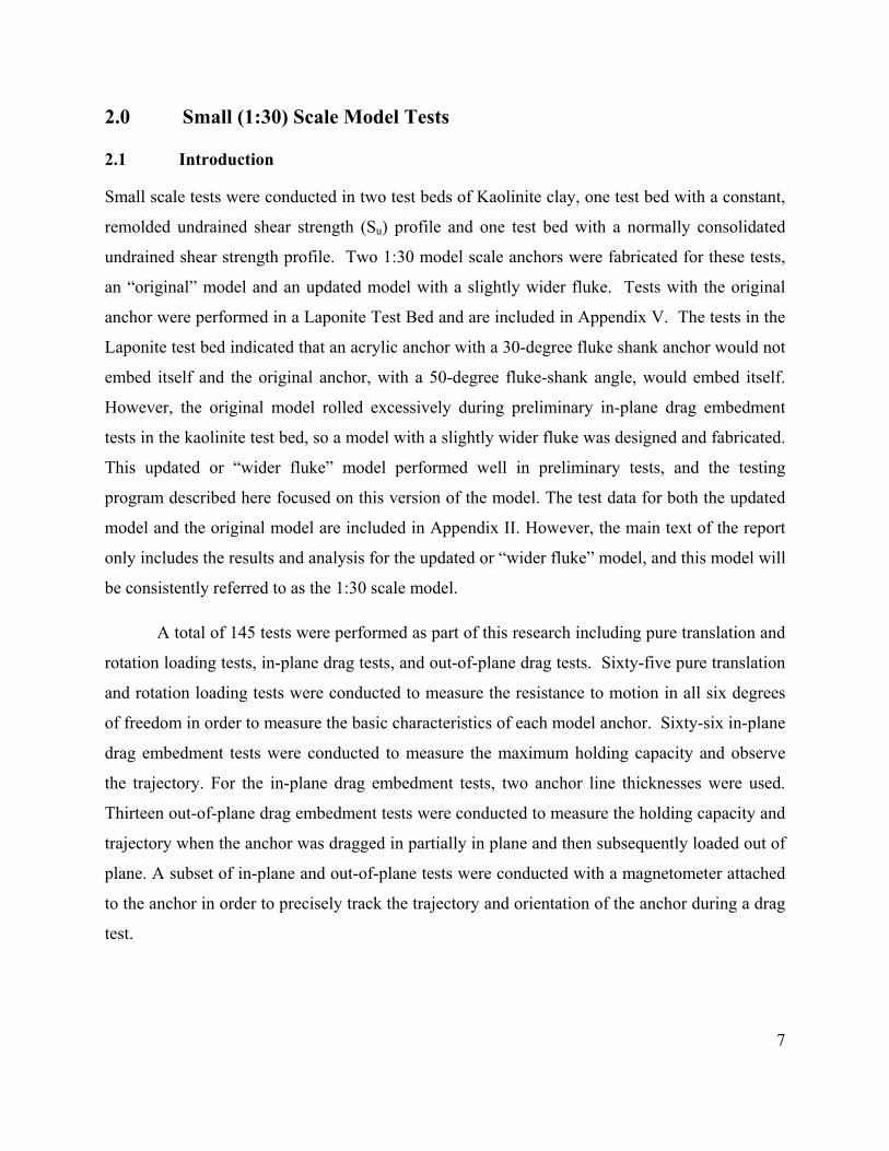
2.2.1.3 Data Acquisition and Control System

The data acquisition and control system was utilized in order to control the test through the

displacement rate of the stepper motor (0.8 in/sec) and to record the output of the motor and load

cell. The system illustrated in Figure 2.4 was composed of two signal conditioning units, a data

acquisition card, a cable adapter between the signal conditioning units and the data acquisition

card, measurement instrumentation, a stepper motor control card with an external wiring and

connection box, and a personal computer. The data acquisition and control system was used to

control the test through the loading device and to acquire and record data from all

instrumentation using a custom-written Labview program named OTRC-SC.VII. Data acquired

11

during the tests was recorded in tab-delimited text files for further analyses. All the electrical

components of the data acquisition system were connected to an Uninterruptible Power Supply

(UPS) system (Model APC Back-UPS 500) to protect the instrumentation and ensure a stable

current. The signal-conditioning boxes and the cable adapter card were grounded to minimize

noise in the measurements (Aubeny et al 2008).

MotorY-axis

Pressure transducersLoad cells

Temperature sensor

LVDTsLMT

Tilt meter

Strain gages

Bridge completion and balance box

Personal computer

Signal conditioning Box 1(Analog Devices 3B Series)

Signal conditioning Box 2(Analog Devices 5B Series)

Cable adapterNI SC 2056

2 Axis stepper/servo motor controller card

NI PCI-7242

DAQ cardNI AT-MIO-64E-3, 6061E

Wiring and connection box for motor control

NI UMI-7764

Two translator drivesSuperior ElectricP/N:SS2000D6

MotorX-axis

Figure 2.4. Data acquisition and control system

2.2.2 Kaolinite Clay

The two soil beds were prepared with water-washed Hydrite T Kaolinite from Dry Branch

Kaolin Company (now IMERYS Kaolin Inc). The soil was prepared by adding water and

12

mixing to achieve the desired water content. The use of kaolinite in laboratory model scale

testing and prototype offshore-foundation tests has been repeatedly reported, due to its

workability, high coefficient of consolidation, and low compressibility (Larsen, 1989; Fuglsang

and Steensen-Bach, 1991; Clukey and Morrison, 1993; El-Gharbawy and Olson, 1999; House

and Randolph, 2001; Clukey and Philips, 2002; Andersen et al., 2003; and Chen and Randolph,

2004). Documentation from the distributor indicates that the specific gravity of the Kaolinite is

2.58 and the mean particle size is 0.7 μm. Index tests indicate that the liquid limit of the clay

ranges between 54% and 58% and the plasticity index ranges between 20% and 26%.

The test beds were prepared by mixing the kaolinite with water to a specific water

content in order to produce a target undrained shear strength (Figure 2.5). The water content of

the test soils ranged from 170% to 60% and corresponded to remolded undrained strength

strengths between 1 psf and 25 psf. A test bed with a constant undrained shear strength versus

depth was created by mixing the soil to the same water content. A test bed of linearly increasing

undrained shear strength with depth was created by placing the soil in layers so that the water

content decreased with depth based on the water content profile for a normally consolidated clay

(e.g., Lee 2008) (Figure 2.5). Immediately after placement, the sensitivity of the soil is one.

Over a period of days to weeks, the undisturbed undrained shear strength increases (Lee 2008).

After several months, the sensitivity of the soil ranges from 1.5 to 2 (El-Sherbiny 2005).

Figure 2.5. Water Content vs. Undrained Shear Strength (Lee 2008)

13

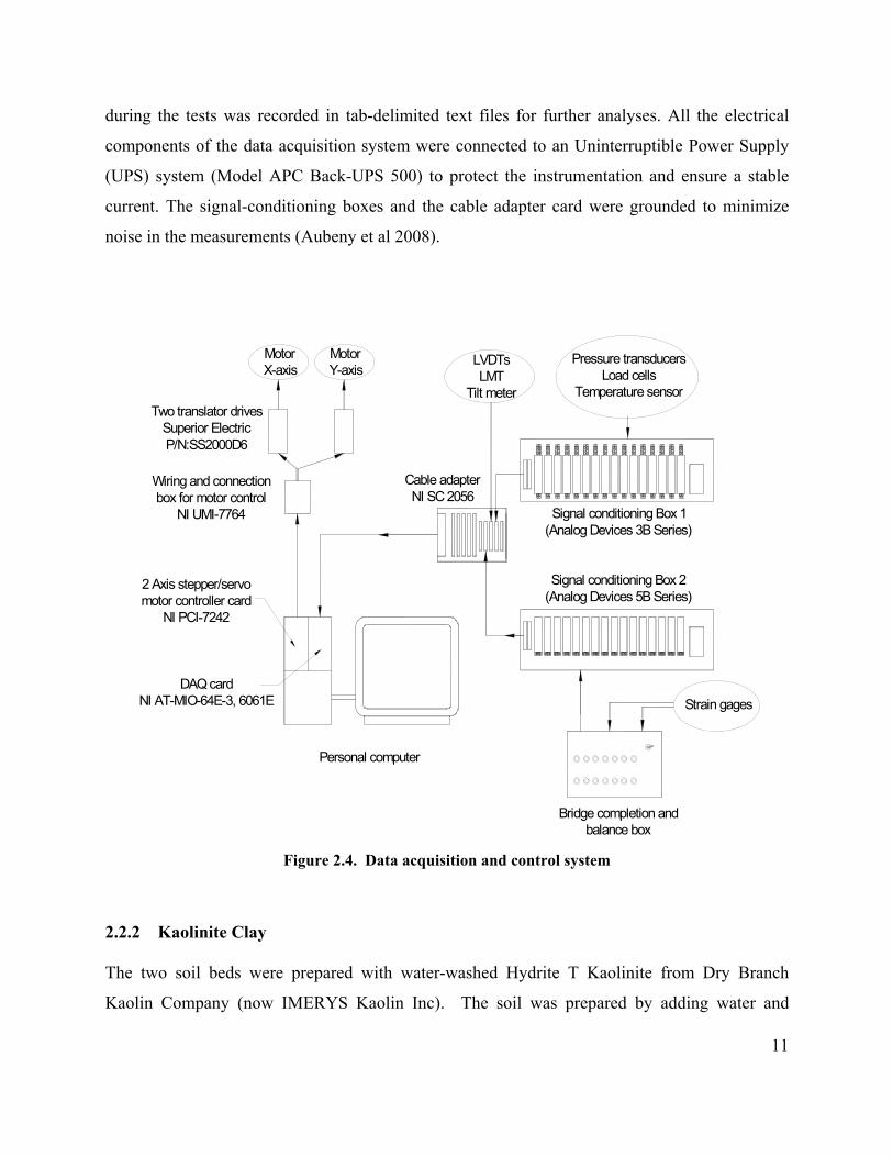
2.2.2.1 T-Bar

The shear strength of the test beds was measured using an in-situ T-bar test. The T-bar is a 1-

inch diameter by 4-inch long acrylic rod (Figure 2.6). The acrylic rod was mounted transversely

on a 3/8 in (9.5 mm) insertion rod that was pushed down into the soil bed at a rate of about 0.8

in/sec (20 mm/s). The measured resistance of the T-bar was corrected for the friction and

bearing of the insertion rod by measuring the resistance of only the insertion rod in a separate

penetration. The undrained shear strength, su, was calculated using the following equation (El-

Sherbiny 2005):

AN

FFs

c

rodtotalu

)( (2.21)

where Ftotal is the total measured resistance during T-bar insertion, Frod is the measured resistance

during separate penetration of the insertion-rod, A is the projected area of the T-bar (4in2 =

2580mm2), and Nc is the bearing capacity factor. The bearing factor, Nc, was used as 10.5

(Stewart & Randolph, 1994), which is the convention in practice at present.

Figure 2.6. T-Bar test

14

2.2.2.2 Thermo-Plastic Tank

The thermo-plastic tank (Figure 2.8) was used for the pure translation and rotation loading tests,

and for in-plane and out-of-plane drag embedment tests with the magnetometer. The thermo-

plastic tank is a Rubbermaid, black, 100-gallon stock tank. The approximate dimensions of the

tank are 4 feet in length, 2 feet in width and 2 feet in height. The Kaolinite in this tank was

mixed and completely remolded each day testing was performed. The mixing was performed

with a steel paddle attached to a drill (Figure 2.7). The undrained shear strength was measured

with the T-bar test and was typically between 10 and 22 psf. For the drag embedment tests

using the magnetometer, the thermo-plastic tank was placed on a wooden platform elevated 40

inches (Figure 2.8) off the reinforced concrete floor and a minimum distance of 42 inches away

from any significant source of metal.

Figure 2.7. Drill with steel paddle and mixing process in the thermoplastic tub

15

Figure 2.8. Thermo Plastic Tank on Elevated Platform

2.2.2.3 Metal Tank

The experimental facility (Figure 2.9) used for in-plane and out-of-plane drag embedment tests

consists of 8-foot wide by 4-foot long by 6-foot deep steel tank. The test bed consisted of a

normally consolidated soil that has an undrained shear strength that increases linearly at 7 to 11

psf/ft. The test bed was placed in layers with water contents that were controlled with depth to

create the normally consolidated clay. For each anchor test, the undrained shear strength of the

test bed was measured using a t-bar test.

16

Figure 2.9 - Testing Facility

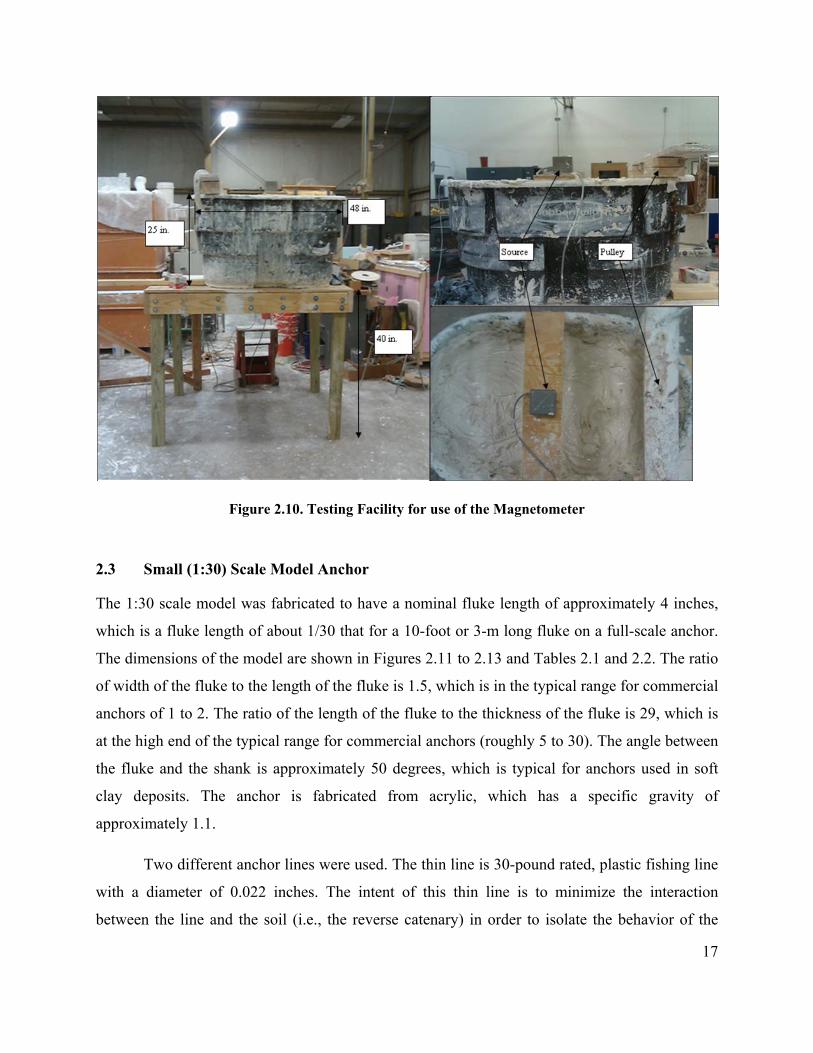
2.2.3 Magnetometer for Tracking In-plane and out-of-plane drag embedment tests were performed with a magnetometer to track

the location and orientation of the anchor. The magnetometer consists essentially of a source and

a sensor. The source emits magnetic fields and the sensor detects the strength and direction of

these magnetic fields. For our tests, the source is stationary and the sensor is attached to the

anchor (at the base of the shank) to track its six degrees of freedom versus time. For testing in

the thermo-plastic tank, the tank was placed on a wooden platform elevated 40 inches off the

reinforced concrete floor and a minimum distance of 42 inches away from any significant source

of metal. Figure 2.10 is a collection of pictures that shows the thermo-plastic tank on the

elevated platform and the location of the source during the test.

17

Figure 2.10. Testing Facility for use of the Magnetometer

2.3 Small (1:30) Scale Model Anchor

The 1:30 scale model was fabricated to have a nominal fluke length of approximately 4 inches,

which is a fluke length of about 1/30 that for a 10-foot or 3-m long fluke on a full-scale anchor.

The dimensions of the model are shown in Figures 2.11 to 2.13 and Tables 2.1 and 2.2. The ratio

of width of the fluke to the length of the fluke is 1.5, which is in the typical range for commercial

anchors of 1 to 2. The ratio of the length of the fluke to the thickness of the fluke is 29, which is

at the high end of the typical range for commercial anchors (roughly 5 to 30). The angle between

the fluke and the shank is approximately 50 degrees, which is typical for anchors used in soft

clay deposits. The anchor is fabricated from acrylic, which has a specific gravity of

approximately 1.1.

Two different anchor lines were used. The thin line is 30-pound rated, plastic fishing line

with a diameter of 0.022 inches. The intent of this thin line is to minimize the interaction

between the line and the soil (i.e., the reverse catenary) in order to isolate the behavior of the

18

anchor alone. The ratio of area of the fluke divided by the square of the line diameter is 21,000.

The thick line is a vinyl-coated galvanized steel wire rope with a diameter of 0.09 inches. This

line thickness is more representative of a typical chain in a field application. For the thick line,

the ratio of area of the fluke to the square of the line diameter is 1,300, which is closer to field

applications where this ratio is on the order of 30 to 150.

Figure 2.11. 1:30 Scale Model Anchor

19

Table 2.1. Physical properties for 1:30 model anchor

Fluke  length 

(longer 

dimension) 

(in.) 

Fluke  length 

(shorter 

dimension) 

(in.) 

Shank 

length 

(in.) 

Fluke‐

Shank 

angle 

(degrees) 

Shank 

height 

(in.) 

Weight 

in  air 

(lbs) 

Volume 

(in.3) 

Thickness 

(in.) 

5.31  3.63  4.31  50 2.38 0.072  1.76  0.13 

Table 2.2. Areas of different surfaces for 1:30 scale model anchor

Area 1 (in2)  Area 2 (in2)  Area 3 (in2) Area 4 (in2) Area 5 (in2) Area 6 (in2)  Area 7 (in2)

0.66  1.03  2.22  0.30 0.80 10.37 2.99 

Figure 2.12. Area 1 through 7 presented in Table 2.2

20

Figure 2.13. Magnetometer attached to 1:30 scale model

2.4 Pure Loading Tests

The pure loading tests characterized the anchor’s resistance to motion in each of the six degrees

of freedom and provide information for the calculation of pure loading bearing capacity factors.

The testing was performed in the thermo-plastic tank which has a constant, remolded undrained

shear strength. Pure loading tests were performed a minimum 12 inches away from the walls of

the thermo-plastic tank so that the anchor and loaded soil around it do not interact with the walls

of the tub and cause boundary problems. Details for these tests are contained in Ganjoo (2010).

2.4.1 Pure Translation Tests

2.4.1.1 Procedure

Pure translation loading test were performed to measure the anchor’s resistance to normal, in-

plane shear, and out-of-plane shear loading. The normal pure loading direction represents a

force being applied perpendicular to the fluke (Figure 2.16). The in-plane shear loading

direction represents a force being applied in the intended loading direction of the anchor (Figure

2.14) (Note: the anchor was inserted down into the soil). The out-of-plane shear loading

direction represents a force applied 90° from in plane loading direction (Figure 2.15). The

undrained shear strength of the tank was measured after the soil was thoroughly mixed and

before the tests began. The anchor was attached to a loading wire or loading rod at one end and

to the load cell at the other end. A loading line was used for the normal test. The loading rod

21

was used for the in-plane and out-of-plane shear test. When the loading rod was used, a separate

test was performed to measure the frictional resistance of the rod. For the in-plane shear loading

test, the anchor was mounted on the loading rod and inserted in to the soil in the manner as the

T-bar test and at a constant rate of 0.8 in/sec. The in-plane shear test with repeated with the

magnetometer sensor attached. For the out-of-plane and normal tests, the soil was removed to a

depth of approximately 10 inches, the anchor was placed at that depth in the desired orientation

and then the soil that was removed was replaced back on top of the anchor (Ganjoo, 2010). The

anchor was pulled out at a constant rate of 0.8 in/sec. The motor displacement and the load cell

readings were recorded throughout the test.

Figure 2.14. In-plane Shear Test Orientation (Left: Just Anchor and Right: With Magnetometer Sensor)

Figure 2.15. Out-of-plane Shear Orientation Figure 2.16. Normal Orientation.

22

2.4.1.2 Results

Twenty-nine pure translational loading tests were performed and the results from the pure

loading test are presented in Appendix II, Tables 1 and 2. The T-Bar Data and Load Cell

Readings versus Motor Line Displacement for each individual test are also presented in

Appendix II. For the 1:30 scale model anchor, nine normal, three in-plane shear, and five out-of-

plane shear loading tests were conducted. For the normal and out-of-plane shear tests, the

resistance listed in the table is the maximum line/rod tension measured. For the in-plane shear

tests, the load recorded was constant with depth, so the resistance recorded is an average of the

load recorded. When the loading rod was used, the friction of the rod was subtracted from the

Load measured during the test. The average undrained shear strength, Su, and the average

resistance of all the tests are presented in Table 2.3.

Table 2.3. Results and analysis of pure translation loading tests for 1:30 scale model

Loading Direction

Average su Average Resistance Bearing Factor

(psf) (lbs) Average Standard Deviation

Range (number of tests)

Normal 10.58 10.65 10.93 0.53 10.42 to 12.02 (9 tests)

In-plane Shear 12.96 3.94 4.22 0.005 4.22 to 4.23 (3 tests)

In-plane Shear with magnetometer sensor attached

12.96 4.19 4.49

0.12 4.35 to 4.57 (3 tests)

Out-of-plane shear 12.03 5.19 6 0.22 5.80 to 6.36 (5 tests)

2.4.1.3 Analysis

The bearing capacity factor accounts for the undrained shear strength (Su) and the anchor

resistance, which facilitates comparison of results from test to test. The following equation was

used to calculate the bearing factor for each pure translation loading direction:

23

(2.1)

where: N = Bearing factor Fmax = Maximum force recorded by the load cell (psf)

Wanchor = Weight of the Anchor (lbs.) Frod = the measured resistance during separate pullout test of the rod (lbs.)

Su = Undrained shear strength (psf) Af = Area of Fluke (ft2)

The bearing factor was calculated for each test performed. The results were consistent

and repeatable as indicated by the average, standard deviation and range of calculated bearing

factor values presented in Table 2.3.

The theoretical bearing capacity was also calculated for each direction. The bearing

capacity was calculated by accounting for the parts on the anchor acting in bearing resistance and

those acting in shear resistance. The irregular geometry of the anchor makes it challenging to

determine whether the area is acting is bearing or shear. This calculation provides an estimate

for comparison with the measured values but should be considered very approximate. In this

calculation, if the area was oriented from 0 to 45° from the loading direction it was considered to

be contributing to the bearing resistance and if it was oriented from 45 to 90° from the loading

direction it was considered to be contributing to the shear resistance. The bearing factor for a

square plate subjected to normal loading is approximately 13 (Aubeny et al 2008). For the side

of fluke (i.e. the thickness) the width of the side is small relative to the length of the bearing area,

so the bearing capacity factor for a buried strip footing of 7.5 is used. The shear resistance is

calculated as the product of an alpha (α) factor, the undrained shear strength, and the area acting

in shear. An α of 1 was used because the soil is completely remolded. There is an opening

between the two legs of the shank; if this area becomes plugged (or clogged) with soil during the

in-plane shear test the plugged zone between the shank legs will act as a normal bearing surface.

For the in-plane shear direction, the calculation was done considering the area between the shank

legs is either unplugged, so the soil passes through that zone during the test, or becomes plugged.

Table 2.4 is a summary of the theoretical and experimental results. Considering the

challenging geometry of the anchor, the theoretical and experimental values are relatively close

(less than 25% difference). The theoretical values tend to be higher than the measured values,

because some areas that are consider to be contributing to the bearing resistance are actually

24

experiencing a combination of shear and bearing resistance. The calculations are shown in Table

2.5.

Table 2.4. Summary of Theoretical and Experimental Bearing Capacity Factors for Pure Translational Loading

Theoretical Bearing Factor Average Experimental Bearing Factor

Normal 13.69 10.93

In-plane Shear 4.68 (unplugged) to 5.91 (plugged)

4.22

Out of Plane Shear 6.02 6.00

25

Table 2.5. Table of Bearing Capacity Calculations: In-Plane Shear – Plugged, In-Plane Shear

Unplugged, Normal and Out-of-Plane Shear

NOTE: For the following table of calculations, Af is the Area of the Fluke and Q(Su) indicates the capacity multiplied by the undrained shear strength, Su. Since the bearing factor is calculated by divided by the Su, the capacity was presented as a function of Su.

Table 2.5a. In-Plane Shear

  Unplugged Shank Plugged Shank 

Bearing Capacity 

Contribution  

Area, A  Nc  Qi (Su) = A*Nc  Area, A  Nc  Qi (Su) = A*Nc 

in2     ft2  in2     ft2 

Area 1  0.66  7.5  0.034 0.66 7.5  0.034

Area 4  0.3  7.5  0.016 0.3 7.5  0.016

Area 5  0.8  13  0.072 2.083984 13  0.188

Shear Contribution  

Area  Nc  Qi (Su) = A*α  Area  Nc  Qi (Su) = A*α 

in2     ft2  in2     ft2 

Area 2  1.03  1  0.007 1.03 1  0.007

Area 2  1.03  1  0.007 1.03 1  0.007

Area 3‐Outside Of Shank 

2.22  1  0.015  2.22  1  0.015 

Area 3‐Outside Of Shank 

2.22  1  0.015  2.22  1  0.015 

Area 3‐In‐side Of Shank 

1.94  1  0.013  ‐  ‐  ‐ 

Area 3‐In‐side Of Shank 

1.94  1  0.013  ‐  ‐  ‐ 

Area 6 ‐Fluke (Bottom) 

10.37  1  0.072  10.37  1  0.072 

Area 6 minus Shank Legs Width(Top) 

10.2  1  0.071  10.2  1  0.071 

 QTotal (Su) = ƩQi 

(Su) 0.337  QTotal (Su) = ƩQi (Su)  0.426 

  N = QTotal(Su)/Su*Af  4.68  N = QTotal(Su)/Su*Af  5.91 

26

Table 2.5b. Normal

Bearing Capacity Contribution  

Area, A  Nc  Qi (Su) = A*Nc 

in2     ft2 

Area 6 (Bottom)  10.37 13 0.936180556 

Shear Contribution  Area  Nc  Qi (Su) = A*α 

in2     ft2 

Area 1  0.66 1 0.005 Area 2  1.03 1 0.007 Area 2  1.03 1 0.007 Area 3  2.22 1 0.015 Area 3  2.22 1 0.015 Area 4  0.3 1 0.002 

Area 5  0.8 1 0.006 

  QTotal (Su) = ƩQi (Su)  0.986 

  N = QTotal(Su)/Su*Af  13.69 

Table 2.5c. Out-of-Plane Shear

Bearing Capacity 

Contribution Area, A  Nc  Qi (Su) = A*Nc 

in2    ft2 

Area 2  1.03 7.5 0.054 Area 2  1.03 7.5 0.054 Area 3  2.22 13 0.200 

Shear Contribution Area  Nc  Qi (Su) = A*α 

in2     ft2 

Area 1  0.66 1 0.005 Area 4  0.3 1 0.002 Area 5  0.8 1 0.006 Area 5  0.8 1 0.006 

Area 6 (Bottom)  10.37 1 0.072 Area 6 (Top‐estimate 2/3 of top fluke is in 

shear) 5.185  1  0.036 

  QTotal (Su) = ƩQi (Su)  0.434 

  N = QTotal(Su)/Su*Af  6.02 

27

2.4.2 Pure Rotation Tests

2.4.2.1 Procedure

A testing apparatus was built to aid the measurement of the rotational resistance of the anchor in

the pitch, yaw, and roll directions (Figure 2.17). A loading line is connected to the stepper motor

and the load cell. Fishing wire is attached to the other side of the load cell, passes through an

aluminum pulley and is connected an acrylic pulley. The acrylic pulley is mounted on top of a

threaded bar and the anchor is attached to the bottom of the threaded rod. The anchor is oriented

differently on the threaded rod depending which degree of rotation was being measured. Figure

2.18 illustrates how the anchor was attached to the threaded rod for each orientation. As the

motor pulls the loading line, the fishing wire makes the acrylic pulley and the anchor rotate. As

the anchor rotates the force is recorded by the load cell. The undrained shear strength was

measured with the T-bar test before each set of rotational tests was performed.

Figure 2.17. Test setup for pure rotational loading test

28

Figure 2.18. Attachment of the Anchor to the Threaded Rod for each Orientation

2.4.2.2 Results

The results from the pure loading test are presented in Appendix II, Tables 1 and 2. The T-Bar

Data and Load Cell Readings versus Motor Line Displacement for each individual test are also

presented in Appendix II. The fishing line tension was measured by the load cell. The average

moment resistance and the undrained shear strength, Su, are presented in Table 2.6 for each type

of rotation.

2.4.2.3 Analysis

In order to analyze the pure rotation motion, the moment needed to rotate the anchor and the

bearing capacity factor was calculated. The moment acting on the anchor is the same as the

moment required to rotate the acrylic pulley. This moment is calculated by taking the product of

the force registered on the load cell and the radius of the acrylic pulley. For calculating the

bearing factor for pure rotation, the equation requires that the Nm value be normalized by the

length of fluke. As the anchors do not have a simple geometry, it is difficult to choose an

equivalent rectangular fluke, so an equivalent square fluke was assumed. An equivalent square

was considered so the calculation would be repeatability. The length of the fluke assuming an

equivalent square was calculated by taking the square root of the area of the fluke. The results

were consistent and repeatable as indicated by the average, standard deviation and range of

moment resistances (Table 2.6). The bearing factor for pure rotation was calculated by the

following equation:

29

(2.2)

where: Nm = Bearing factor for pure rotation M = Moment applied on the anchor, where: M = Favg*r F= the average force recorded by the load cell r = radius of the pulley Su = Undrained shear strength L = Length of fluke, assuming the anchor fluke is an equivalent square

= Af = Area of Fluke

Table 2.6. Results and Analysis of Pure Rotational Loading Tests

Rotational Loading Direction

Undrained Shear Strength, Su (psf)

Moment Resistance (in-lb) Average Bearing Factor (Assuming Square Fluke)

Average Standard Deviation Range

Pitch 9.97 5.54 0.11 5.48 to 5.75 2.4

Roll 10.86 3.25 0.04 6.45 to 6.57 2.58

yaw 9.67 2.25 0.07 4.22 to 4.38 1.92

2.5 Drag Tests

In-plane and out-of plane drag tests were performed in the metal tank, which has a normally

consolidated undrained shear strength profile. The tests were performed on one of three tracks in

the metal tank (Figure 2.19). The track locations were determined by the pulley locations on the

loading frame. The soil in the metal tank has a sensitivity of 1.5 to 2. Several tests were

performed on the same track in the same day, so it is expected that soil along the track remolded

during the various tests.

Select in-plane and out-of-plane drag tests were performed in thermo-plastic tank, which has

a constant, remolded undrained shear strength. These tests were performed to demonstrate the

use of the magnetometer and confirm the general trajectory that was observed in the metal tank

drag tests.

30

Figure 2.19. Testing Tracks in Metal Tank

2.5.1 In-plane drag embedment tests

2.5.1.1 Procedure

For the drag embedment tests, the model anchor was placed at the mudline with the shank

oriented horizontally. The anchor line was attached at the shackle point on the anchor, and then

loaded by the motor. In-plane drag embedment tests with the 1:30 scale model were performed

with one of two anchor loading lines. The thick loading line has a diameter, b, of 0.09 in

(Af/b2=1300) and the thin anchor line has a diameter, b, of 0.022 in (Af/b

2=21,000). The anchor

line passes through a pulley located approximately 72 inches in away from the starting point and

approximately inches 6 inches above the mudline, such that the load angle is initially about 5°

and then gradually becomes steeper as the anchor becomes embedded (Figure 2.20). The

maximum embedment was typically noted approximately 40 inches from the start of the test or

approximately 30 inches from the pulley, which indicates that the anchor line angle was

approximately 25° (Figure 2.20). The tension in the anchor line is measured by a load cell that is

31

located on the anchor line after it passes through the pulley. The motor displacement and the

anchor line tension are measured and recorded as the anchor moved through the soil. In order to

better understand the trajectory, tests were conducted run where the anchor was stopped

periodically throughout the drag distance and a rod was used to measure the depth of embedment

and its horizontal location. In most tests, the test was stopped just after the maximum load cell

reading was reached, and the maximum load and the depth of embedment were recorded.

Additional in-plane drag test were conducted where the anchor line was significantly

steeper than in the procedure noted above. The starting point is approximately 37 inches away

from the pulley, so that the load angle is initially about 10° and then becomes steeper as the

anchor becomes embedded (Figure 2.22). The thick loading line was used for these tests.

In-plane drag embedment tests with the magnetometer were conducted in the thermo-

plastic tank, which has a constant, remolded shear strength. The magnetometer sensor was

attached to the anchor during the test (Figure 2.13). The anchor line was pulled by the stepper

motor or by hand. The tension in the anchor line was measured and trajectory orientation data

was collected.

Figure 2.20. Example Test Configuration for In-Plane Drag Embedment Test

32

2.5.1.2 Results

The anchor line tension, the motor displacement and the maximum embedment is recorded

during each test. The holding capacity is noted as the maximum anchor line tension.

Corrections to the holding capacity are discussed in the Analysis Section 2.5.1.3. When the

maximum is presented as a function of the length of the fluke, the shorter dimension of the fluke

length is used: 3.625 for the 1:30 scale model anchor (see Table 2.1).

The tests performed with the 1:30 scale model anchor include the use of a thick loading

line, a thin loading line, steep loading angles, and the magnetometer. All the results for the T-bar

tests and the load cell readings versus motor line displacement are presented in Appendix II. The

data is also summarized in Appendix II in Tables 3 through 6. The trajectory data for these tests

is presented in Figure 2.21.

Figure 2.21. Trajectory of an In-Plane Drag Embedment Tests

33

2.5.1.2.1 Thick Loading Line

The T-bar data and load cell readings versus motor line displacement for each individual test are

presented in Appendix II, and the results are summarized in Appendix II, Table 2. Twenty-one

tests were performed with the 1:30 scale model anchor and a thick loading line. With the thicker

loading line, the 1:30 scale model anchor tended to dive down to a depth of about 2.7 times the

length of fluke (approximately 9.3 inches) and achieve a holding capacity that was 40 to 60 times

its weight in air (note that the specific gravity of the acrylic is about seven times smaller than that

for steel, so these holding capacities are the equivalent of 6 to 9 times its weight for a steel

anchor, neglecting the effect of its weight on the holding capacity). The trajectory of the anchor

was measured in three tests with the thick loading line is shown in Figure 2.21.

2.5.1.2.2 Thin Loading Line

The T-bar data and load cell readings versus motor line displacement for each individual test are

presented in Appendix II, and the results are summarized in Appendix II, Table 4. Four tests

were performed with the 1:30 scale model anchor and a thin loading line. With the thin loading

line, the 1:30 scale model anchor tended to dive down to a depth of about 3.6 times the length of

fluke (approximately 13 inches) and achieve a holding capacity that was 50 to 60 times its

weight (these holding capacities are the equivalent of 7 to 9 times its weight for a steel anchor).

The measured trajectory of the anchor with the thin line is shown in Figure 2.21.

2.5.1.2.3 Steep Loading Angles

The T-bar data and load cell readings versus motor line displacement for each individual test are

presented in Appendix II, and the results are summarized in Appendix II, Table 5. Three tests

were performed with the 1:30 scale model anchor and steep loading angles. With the loading line

relatively steep, the 1:30 scale model anchor tended to dive down to a depth of about 1.4 times

the length of fluke (approximately 6.5 inches) and achieve a holding capacity that was on 38 to

50 times its weight (these holding capacities are the equivalent of 5 to 7 times its weight for a

steel anchor). The trajectory of the anchor was measured in the first test to determine point of

maximum embedment (Figure 2.21). In Figure 2.22, the trajectory is illustrated for both the

embedment and for the anchor pullout in order to observe what anchor line angle would cause

the anchor to pull out.

34

Figure 2.22. Illustration of In-plane Drag test with Steep Anchor Line

2.5.1.2.4 Results with Magnetometer

Testing with the magnetometer has provided valuable information on the trajectory of the anchor

and how it is affected by the initial pitch orientation of the anchor. The T-bar data and load cell

readings versus motor line displacement for each individual test are presented in Appendix II,

and the results are summarized in Appendix II, Table 6. An illustration of the in-plane drag tests

with the magnetometer is presented in Figure 2.23. There were 10 tests conducted with the

magnetometer with the 1:30 scale model anchor. The test results from a representative in-plane

drag test are presented in Figure 2.24. The anchor embedded itself from the starting point 1.4 in

to 5.6 in (1.2 fluke lengths) at the maximum embedment, after which it began to pullout. The

distance between the start of the test and the pulley is approximately 40 inches in the thermo-

plastic tank, as compared with 72 in. in the metal tank, such that the anchor line angle increases

faster in the thermo-plastic tank which reduces the embedment of the anchor. In the thermo-

plastic tank, the anchor started to reduced embedment and pullout at a distance of approximately

15 inches from the pulley or at an anchor line angle of approximately 25°. In the metal tank, the

35

maximum embedment was typically noted approximately 40 inches from the start of the test or

approximately 30 inches from the pulley, which would indicate that line angle was

approximately 25°; the geometry in the two test beds is consistent. The pitch of anchor was

approximately -35° (diving) at the start of the test and was approximately -10° (diving) at the

maximum embedment. The anchor rolled from 0° at the start of the test to about -10° (to the

right) at the maximum embedment. When the anchor was being pulled out, the anchor continued

to roll up to -20° (to the right). The anchor yawed from 0° at the start of the rest to 5° at the

maximum embedment. The anchor line angle is estimated to be 25° when the anchor began to

pull out. The load is relatively constant after 10 inches of drag distance (X), which is expected

since the soil strength is constant.

Figure 2.23. Illustration of In-plane Drag Test with Magnetometer

36

Figure 2.24. Out-of-plane drag test data with the Magnetometer

37

Preliminary testing with the magnetometer has been conducted on the effect of the initial

pitch angle on the trajectory of the anchor. The testing indicates that regardless of the initial

pitch angle, θf, the anchor adjusts to a similar path after a relatively short drag distance. Figure

2.25 shows tests that were conducted with an initial pitch angle of 30, 40, 60, and 80°. This plot

indicates that after 5 inches (1.4 fluke lengths) of drag distance (X) that the general pitch trend of

all the tests converges and the trajectory is becomes very similar for all the tests. Figure 2.25

shows that trajectory (drag distance vs. embedment) is very similar for all the tests conducted.

Figure 2.25. Effect of Initial Pitch Angle on Pitch and the Trajectory

38

2.5.1.3 Analysis

The following is a discussion of the corrected holding capacity, the uncertainty in the measured

and calculated values, and the calculation of the bearing capacity factor (Ne).

The tension in the anchor line is measured at the load cell which is oriented vertically and

located after the anchor line passes through a pulley (Figure 2.20). The vertical tension

measured by the load cell, Tv, is less than the anchor line tension at the mudline, To due to the

resistance introduced be the pulley. The measurements comparing the two values indicate that

To = 0.8 Tv for the thick line and To = 0.9 Tv for the thin line. The holding capacity was corrected

using this factor.

The holding capacity is defined as the maximum load cell reading registered during the

drag embedment test. Figure 2.26 displays two graphs of load cell readings versus line

displacement of the motor. The trajectory was not measured for these particular tests, but it was

measured for another test on the same day. The trajectory measurements were interpolated to be

presented on the graphs below. Typically, the maximum load cell reading corresponded very

closely with the final embedment measured at the end of the test, as seen in the plot from

2010/07/12_IP_Track2_3. In some tests, the maximum load cell reading occurred at a shallower

depth than the final embedment, as seen in the plot from 2010/06/24_IP_Track3_4. Since there

is very limited data on the trajectory for in-plane drag tests and interpolating the results is

unreliable, the final embedment is noted as the depth of the anchor recorded at the end of the test

and the holding capacity is noted as the maximum load cell reading.

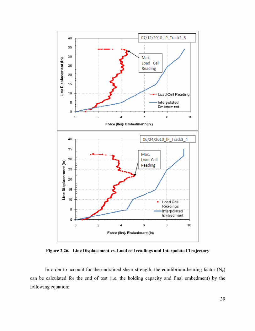
39

Figure 2.26. Line Displacement vs. Load cell readings and Interpolated Trajectory

In order to account for the undrained shear strength, the equilibrium bearing factor (Ne)

can be calculated for the end of test (i.e. the holding capacity and final embedment) by the

following equation:

40

(2.3)

where Ne = Equilibrium bearing factor Ta = Tension of the anchor line at the shackle point Su = Undrained shear strength at the Fluke Af = Area of Fluke

There is uncertainty in the value of the undrained shear strength (Su) at the final

embedment of the fluke since the Su in the test bed varies spatially along the test track, it varies

irregularly with depth, and it varies from test to test on the same day. The undrained shear

strength profiles for the same track on the same day were used to establish an average shear

strength gradient (k) and strength at the mudline (Su0) (Figure 2.27). The final embedment of the

anchor was measured at the end of the test with a ruler, which is not a precise measurement and

does not consider the orientation of the anchor. The undrained shear strength of the test bed was

measured before the in-plane drag embedment tests were conducted on a given day, and the soil

shear strength likely decreased with additional pulls along the track during that day. Therefore,

the estimated values for Su are approximate for all tests; the estimated values used for the first

pull on a track for a given day are likely the most representative of what existed at the time of the

drag test.

41

Figure 2.27. Example of Undrained Shear Strength Profile

In order to calculate Ne, the tension at the shackle, Ta, was estimated from the tension at

the mudline To using the Nuebecker and Randolph (1995) model for reverse catenary. An

example in-plane drag embedment test from the metal tank, Test 7/12/2010_IP_Track2_2, is

used here to illustrate this analysis. The undrained shear strength was 0.8 psf at the mudline and

was increasing at 8 psf/ft and the line was the thick line. The tension at the shackle point, Ta, is a

function of the geometry of the anchor line at the shackle point. From the geometry of the test,

shown in Figure 2.20, it can be estimated that if the anchor line was completely taut that the

anchor line angle with the mudline, θo and the anchor line angle at the shackle, θa, would be 24°.

The final embedment from the mudline to the fluke was 9 inches and from the geometry of the

anchor it is estimated that the depth to the shackle point was 6.625 inches. The load cell reading,

TV, at the final embedment was 3.80 lbs, which makes To=3.04 lbs. If we consider the reverse

catenary forming between the anchor line at the shackle and the anchor line where it exits the

42

soil, when θo is 24°, θa would be 28°. The pitch of the fluke, θf, can be calculated using the

following equation and the results are display in Table 2.7.

θf = θaf - θa =cos-1 (Nsmax / Ne) - θa (2.4)

where Nsmax = Bearing factor for in-plane shear Ne = Equilibrium Bearing factor θf = Pitch of the Fluke

θa = anchor line angle at the shackle θaf = Sum of the pitch of the fluke and the anchor line angle at the shackle

The estimated pitch, θf is 17.9° (indicating the anchor still in a diving position).

Table 2.7. Comparison of Ta and Ne

It is important to note that whether To=Ta or Ta is adjusted for the reverse catenary of the

anchor line that the change in Ne is less than 5%. Since the difference between To and Ta is

small, and many assumptions need to be made to calculate Ta, the “Line Load at Mudline (Final

Embedment)” reported in the Tables 3 through 7 of Appendix II is To. For the calculation of the

equilibrium bearing capacity factor, Ne, the tension used in that equation is To instead of Ta.

When To is used to calculate Ne, it is designated as Ne* and indicates that value is an

overestimation of the value of Ne.

The data obtained from the magnetometer in the thermo-plastic tank indicates that the

pitch of the anchor at the maximum embedment is approximately 10 to 15° (in a diving position).

This observation is generally consistent with the calculations discussed above, where the pitch is

calculated to be 17.9°. Though there are differences in the testing geometry and the undrained

shear strength profile, the angle of the anchor line (assuming the line is taut) at the maximum

embedment is approximately 26°, which is close the calculated angle of 24° for the in-plane tests

Condition θo (deg) θa (deg) θaf (deg) θf (deg) Tension in

line, T (lbs) Ne

(Eqn. 2.3)

Anchor line completely taut

24 24 47.4 23.4 To=Ta=3.04 6.21

Anchor line forming a reverse

catenary 24 28.0 45.9 17.9 Ta=2.96 6.04

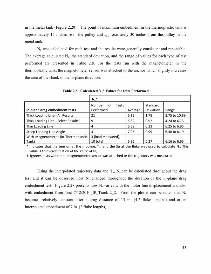
43

in the metal tank (Figure 2.20). The point of maximum embedment in the thermoplastic tank is

approximately 15 inches from the pulley and approximately 30 inches from the pulley in the

metal tank.

Ne was calculated for each test and the results were generally consistent and repeatable.

The average calculated Ne, the standard deviation, and the range of values for each type of test

performed are presented in Table 2.8. For the tests run with the magnetometer in the

thermoplastic tank, the magnetometer sensor was attached to the anchor which slightly increases

the area of the shank in the in-plane direction.

Table 2.8. Calculated Ne* Values for tests Performed

   Ne*

In‐plane drag embedment tests Number  of  Tests Performed Average

Standard Deviation  Range 

Thick Loading Line ‐ All Results  21 6.19 1.78  3.75 to 10.89

Thick Loading Line ‐ Select Results1  9 5.82 0.92  4.24 to 6.73

Thin Loading Line  4 6.58 0.33  6.25 to 6.95

Steep Loading Line Angle  3 7.05 0.99  6.48 to 8.19

With Magnetometer  (in Thermoplastic Tank) 

3 (load measured), 10 total 6.35 0.27  6.16 to 6.65

*  Indicates  that  the  tension at  the mudline, To, and  the Su at  the  fluke was used  to calculate Ne. This value is an overestimation of the value of Ne 

1. Ignores tests where the magnetometer sensor was attached or the trajectory was measured

Using the interpolated trajectory data and To, Ne can be calculated throughout the drag

test and it can be observed how Ne changed throughout the duration of the in-plane drag

embedment test. Figure 2.28 presents how Ne varies with the motor line displacement and also

with embedment from Test 7/12/2010_IP_Track 2_2. From the plot it can be noted that Ne

becomes relatively constant after a drag distance of 15 in. (4.2 fluke lengths) and at an

interpolated embedment of 7 in. (2 fluke lengths).

44

Figure 2.28. Ne vs. Line Displacement and Embedment Depth

The ratio of the change in displacement normal to the fluke (dn) to the change in

displacement parallel to the fluke (ds) is usually small for DEA (Aubeny 2010a). Testing with

the magnetometer indicated that the value of dn/ds for this testing is approximately 0.2 after 1-3

fluke length of drag distance (Figure 2.29). Since dn/ds is greater than 0, the embedment in these

tests is reduced compared to a typical DEA.

Figure 2.29. Variation in dn/ds throughout Drag Distance

45

2.5.2 Out-of-plane Drag Embedment Tests

2.5.2.1 Procedure

Out-of-plane drag embedment tests were run by initially embedding the anchor with an in-plane

drag, then changing the angle of the anchor line and dragging the anchor out-of-plane. The out

of plane angle was either 15° or 25°. For the out-of-plane angle of 15°, the in-plane test was run

on Track 1 and then the pulley was re-located to Track 2 for the out-of-plane portion of the test

(Figure 2.20). For the out-of-plane angle of 25°, the in-plane test was run on Track 1 and then

the pulley was re-located to Track 3 for the out-of-plane portion of the test (Figure 2.20). The

undrained shear strength, Su, in the metal tank differs between the track locations and in between

the track locations because the track locations are regularly disturbed by in-plane drag

embedment tests. The changes in Su affected the results of the out-of-plane tests. During the in-

plane portion of the test, the anchor was embedded either one fluke length or to the maximum

embedment depth observed in previous in-plane tests. The motor displacement and tension in

the line were measured as the anchor moved through the soil. In order to better understand the

trajectory, a test was run where the anchor was stopped periodically throughout the drag and a

rod was used to measure the depth of embedment and its horizontal location. The anchor line

was 0.09 in. in diameter and appeared to be close to taut in both in-plane and out-of-plane

portions of the tests.

Out-of plane tests with the magnetometer were conducted in the thermo-plastic tank,

which has a constant, remolded undrained shear strength. The magnetometer was attached to the

anchor during the test. Due to the size restraint of the tank the anchor was not “installed” with an

in-plane drag test. The anchor was embedded by hand approximately 1 fluke length and was

oriented out-of-plane of the line of action. The tension in the anchor line was measured and

orientation data was collected.

2.5.2.2 Results

Generally, the anchor with the 1:30 scale model aligned with line of action when it was pulled

out of plane. There was some rolling observed in the out of plane tests, but despite the rolling

the anchor tended to continue to embed into the soil. All the results for the T-bar tests and the

load cell readings versus motor line displacement are presented in Appendix II. The data also

summarized in Appendix II in Tables 8 through 10.

46

2.5.2.2.1 “Installed” to the Expected Maximum Embedment

The T-bar data and load cell readings versus motor line displacement for each individual test are

presented in Appendix II, and the results are summarized in Appendix II, Table 8. Seven tests

were performed where the anchor was installed to the expected maximum embedment and then

the anchor line was oriented 25° out of plane. When anchor line direction changed, the angle of

the anchor line with the mudline changed from 14° at the end of in-plane to 12° at the beginning

of the out of plane, which could have caused the anchor to dive deeper and impacted the

trajectory of the anchor. The maximum embedment at the end of the out-of-plane test was

approximately 2.4 times the length of fluke (8.6 inches) and achieved a holding capacity that was

80 to 100 times its weight in air (these holding capacities are the equivalent of 11 to 14 times its

weight for a steel anchor).

2.5.2.2.2 “Installed” One-Fluke Length

The T-bar data and load cell readings versus motor line displacement for each individual test are

presented in Appendix II, and the results are summarized in Appendix II, Table 9. Three tests

were performed where the anchor was installed to one fluke length and then the anchor line was

oriented 25° out of plane. When anchor line direction changed, the angle of the anchor line with

the mudline changed from 10° at the end of in-plane to 9° at the beginning of the out of plane,

which caused the anchor to dive slightly more than in a typical in-plane test. The maximum

embedment at the end of the out-of-plane test was approximately 3 times the length of fluke

(10.8 inches) and achieved a holding capacity that was 70 to 90 times its weight in air (these

holding capacities are the equivalent of 11 to 13 times its weight for a steel anchor). An example

of the trajectory presented below in Figure 2.30.

47

Figure 2.30. Trajectory for Out-of-plane Test

2.5.2.2.3 Results with Magnetometer

The T-bar data and load cell readings versus motor line displacement for each individual test are

presented in Appendix II, and the results are summarized in Appendix II, Table 10. Figure

2.30presents the load cell readings and the orientation data for an out-of-plane load test. The

anchor was oriented 30° out-of-plane at the start of the test. Initially, the anchor was embedded

approximately 1 fluke length, oriented with a pitch of -20° and a yaw of 30° (out-of-plane angle).

The yaw angle starts at approximately 30° and approaches 0° after 5-10 inches of drag,

indicating that the anchor aligned with the line of action. Three tests were conducted with the

magnetometer at out-of-plane angles for demonstration.

48

Figure 2.28. Out-of-plane drag test data with the Magnetometer.

2.5.2.3 Analysis

The load cell readings were corrected for the pulley resistance to yield the anchor line tension at

the mudline (To = 0.8 Tv). The bearing capacity factor was calculated in the same manner as the

in-plane drag tests. The undrained shear strength, Su, of the soil in the metal tank differs

49

between the track locations and in between the track locations because the track locations are

regularly disturbed to run in-plane drag embedment tests. The uncertainty in the value of Su

throughout the trajectory affected the load cell readings and the selection of the appropriate Su to

use in the Ne calculation. One observation that should be noted is that the anchor line appeared

to be taut in the out-of-plane portion of the test. The anchor tended to turn very quickly into the

line of action of the anchor line. The average calculated Ne, the standard deviation, and the

range of values for each type of test performed are presented in Table 2.9. The calculated values

of Ne tend to be 5 to 10% higher than the in-plane drag embedment tests, which may be due to

the variation in Su throughout the tank. The tests with the magnetometer were performed for

demonstration and only one test was conducted at each out of plane orientation: 30°, 60°, and

90°.

Table 2.9. Out of Plane Ne Values for Tests Performed

  Ne* 

Out‐of‐plane drag embedment tests Number  of  Tests Performed Average

Standard Deviation  Range 

"Installed"  to  Expected  Maximum Embedment ‐ All Tests  6 6.3 1.02  5.30 to 8.08

"Installed"  to  Expected  Maximum Embedment ‐ Select Test1  3 6.05 0.65  5.57 to 6.79

"Installed" to One Fluke Length  3 5.9 0.84  5.10 to 6.78

*Indicates that the tension at the mudline, To, and the Su at the fluke was used to calculate Ne. This value is an overestimation of the value of Ne  

1. Ignores tests where the anchor line slipped off pulley 

50

3.0 Large-Scale Tests

3.1 Introduction

Drag embedment anchors (DEAs) are the most utilized anchor for mooring floating

mobile offshore drilling units (MODUs) in the Gulf of Mexico. During hurricane Ike in 2009

there were several failures in MODU mooring systems that caused MODUS to leave station.

During hurricanes Ivan (2004), Katrina (2006), and Rita (2006), seventeen MODUs lost station

keeping. Anchors were dragged during some of these MODU mooring failures and are

suspected to have caused several instances of pipeline damage.

The objective of large scale testing is to better understand the performance of drag

embedment anchors and improve the design and increase the overall reliability of DEAs for

mooring MODUs. A generic DEA model was constructed by Delmar Systems and was used for

all the in-plane, out-of-plane, and break-out tests in the large scale testing conducted in the

towing tank at the Haynes Laboratory at Texas A&M University.

3.2 Experimental Test Arrangements

Large-scale tests (scale ~ 1:10) of the performance of the drag embedment anchor (DEA)

were conducted in the dredge/tow tank in the Haynes Coastal Engineering Laboratory at Texas

A&M University. Both in-plane and out-of-plane performance of DEAs were investigated. The

dredge/tow tank is 45.6 m (149.5 ft) long, 3.66 m (12 ft) wide, and a maximum water depth of

3.05 m (10 ft). The dredge/tow tank has a sediment pit that is 7.6 m (25 ft) long, 3.7 m (12 ft)

wide, and 1.5 m (5 ft) deep as shown in Figure 3.1. The dredge/tow carriage is capable of speeds

up to 2 m/s (4 kts) and has a vertical ladder that can move vertically and horizontally. The ladder

is instrumented to measure the load on the ladder up to 1364 kg (3000 lb) or it can be fixed such

that it doesn’t move and carry a much greater weight. There are also windows located in the

region of the sediment pit that are useful in flow visualization studies in the vicinity of the

sediment pit. A suitable material was selected to be placed in the sediment pit to represent the

seafloor. The dredge/tow carriage was in place in the tank to provide the forces needed to drag

the anchors. The size of the facility allowed testing of models that were ~ 1-2 feet wide.

Procedures were developed and instrumentation acquired to measure the anchor location (x, y

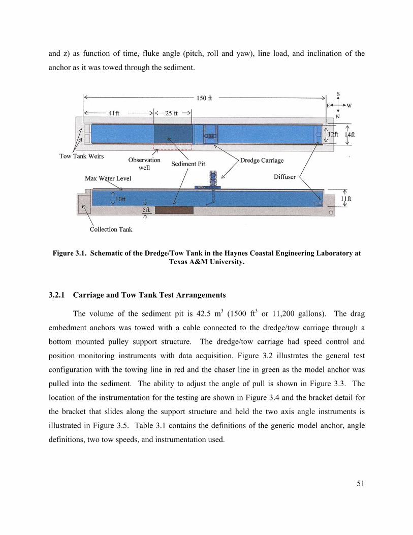
51

and z) as function of time, fluke angle (pitch, roll and yaw), line load, and inclination of the

anchor as it was towed through the sediment.

Figure 3.1. Schematic of the Dredge/Tow Tank in the Haynes Coastal Engineering Laboratory at Texas A&M University.

3.2.1 Carriage and Tow Tank Test Arrangements

The volume of the sediment pit is 42.5 m3 (1500 ft3 or 11,200 gallons). The drag

embedment anchors was towed with a cable connected to the dredge/tow carriage through a

bottom mounted pulley support structure. The dredge/tow carriage had speed control and

position monitoring instruments with data acquisition. Figure 3.2 illustrates the general test

configuration with the towing line in red and the chaser line in green as the model anchor was

pulled into the sediment. The ability to adjust the angle of pull is shown in Figure 3.3. The

location of the instrumentation for the testing are shown in Figure 3.4 and the bracket detail for

the bracket that slides along the support structure and held the two axis angle instruments is

illustrated in Figure 3.5. Table 3.1 contains the definitions of the generic model anchor, angle

definitions, two tow speeds, and instrumentation used.

52

Figure 3.2. General test configuration with the main pull line (grey) and data acquisition chaser line (dashed).

Figure 3.3. Pull angle adjustments

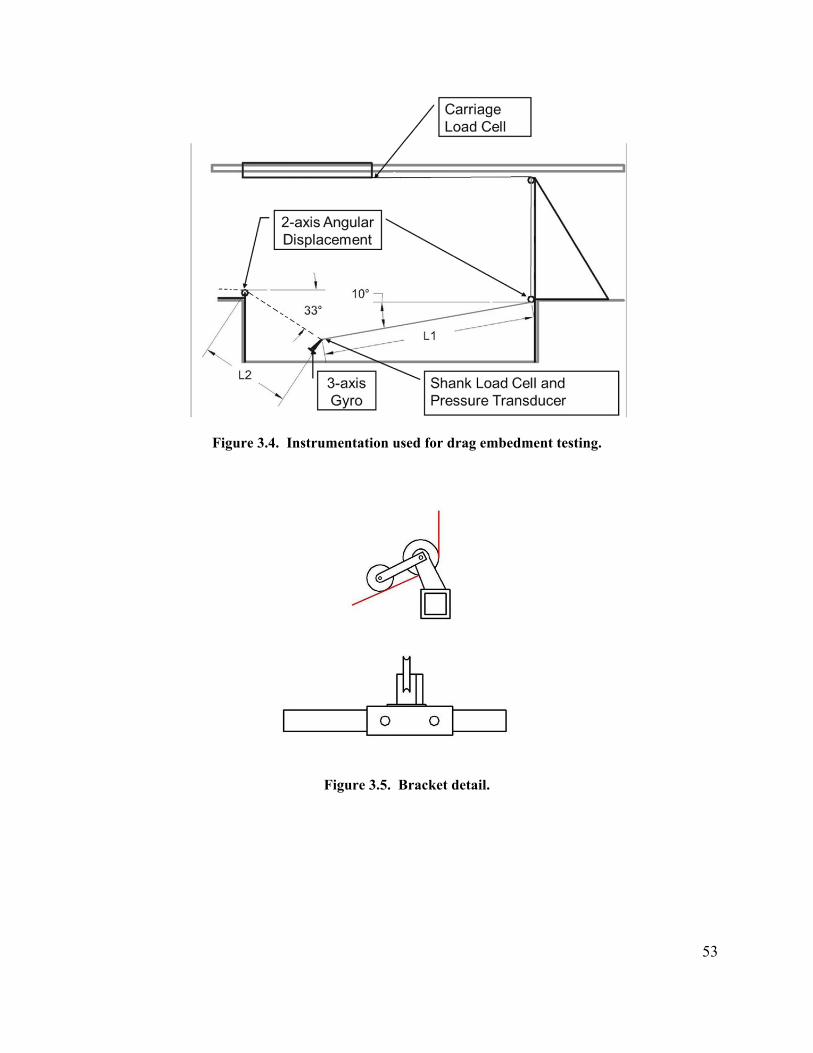
53

Figure 3.4. Instrumentation used for drag embedment testing.

Figure 3.5. Bracket detail.

54

Table 3.1. Definitions and characteristics of generic model anchor and instrumentation.

Chaser angle V – vertical angle of chaser wire Chaser angle H – horizontal angle of chaser wire Chaser displacement – displacement of chaser line connected to anchor shank Anchor angle V – vertical angle of tow line at pulley Anchor angle H – horizontal angle of tow line at pulley Diameter of tow line, data cable, chain bundle is 0.75 inches Speed – 0.42 ft/s; 0.13 m/s (equivalent prototype speed of 2 fluke lengths/min) Speed – 0.62 ft/s; 0.19 m/s (equivalent prototype speed of 3 fluke lengths/min) Pressure – depth of anchor in ft of mud measured by pressure gauge mounted on underside of fluke. Inclinometer Pitch – measured by inclinometer on underside of fluke Inclinometer Roll – measured by inclinometer on underside of fluke Anchor force – force measured by load cell attached between tow line and anchor shank (lb) Carriage force - force measured by load cell attached between tow line and carriage (lb) Vertical distance between mud line and chaser pulley is 2.7 ft

3.2.2 Sediment Pit Layout and Global Coordinates

An initial 6 inch layer of sand was placed in the bottom of pit. The sand layer was used

as a safety depth gauge, it was predicted that as the anchor transitioned into the sand layer the

force transducers would spike indicating to the operators to shut down the system, thus

preventing damage to the anchor and the instrumentation. The mud test mixture was made on

site using a motorized cement mixer and standard 5 gallon buckets to measure the desired

amounts of sand, bentonite and water and the setup is shown in Figure 3.6. The desired sediment

mixture was 50% sand, 50% bentonite, and 125% water that resulted in 2.2 buckets of sand, 2.5

buckets of bentonite, and 7.7 buckets of water. The ¾ cubic yard dump bucket via the overhead

crane placed the mud mixture into the sediment pit until it reached a depth of 6 inches below the

flume to pit transition line.

55

Figure 3.6. Sediment mixture operation outside and discharging sediment into sediment pit in the

towing flume.

There is a shadow zone to note, existing in the western most edge of the sediment pit,

where the mixer was unable to reach as illustrated in the right hand side of Figure 3.7. However,

this area was expected and therefore used as the anchor initial placement site, which being on the

surface has little effect on the tests. The sediment pit layout and support structure for the towing

line and chaser line are shown in Figure 3.8. The geotechnical characteristics of the mud mixture

in the sediment pit are tabulated Table 3.2 and show the mixture was close to the 50% sand, 50%

bentonite, and 125% water goal.

Figure 3.7. Sediment pit global coordinates and profile.

56

Table 3.2. Sediment pit sand, bentonite, and water percentages and bulk density.

Date Sand (%) Bentonite (%) Water (%) Bulk density (lb/ft3) March 10, 2010 East End of Pit

48.4 51.6 128.2 86.17

March 10, 2010 West End of Pit

50.2 49.8 120/7 87.30

May 27, 2010 51.6 48.4 112.7 88.07

Figure 3.8. Support structure and sediment pit.

3.2.3 Sediment (Mud) Mixing Device

A mud mixing device was constructed and replaced the original dredge cutter head on the

ladder’s articulating arm. The mixer operates at a 40° angle to horizontal to a depth of 4 ft. The

2-foot diameter mixer was operated at approximately 12 RPM. The mixer as shown in Figure

3.9 was used extensively to unify the mud matrix and break up any clumps and had an additional

benefit of leveling the mud surface. It produced only minor peaks and valleys after optimizing

and semi-automating the mixing procedure. The overlapping paths after a recent mixing are

shown in Figure 3.10.

57

After a period of approximately one week of daily mixing and soil strength tests, trial

runs of in-plane tests were conducted. This determined that between four to six anchor tows

would be utilized without their paths crossing into disturbed zones. After which, the mixer was

used to uniformly disturb the mud pit in preparation for additional tows. This procedure carried

on throughout the testing.

Figure 3.9. Sediment mixing device.

Figure 3.10. S sediment surface after recent mixing.

3.2.4 Anchor and towline characteristics

The 1:10 length scale generic anchor was constructed and provided by Delmar. Figure

3.12 lists the overall geometry, in addition to the fluke plate centroid. The centroid location was

used to determine the three adjustable fluke to shank angle settings of 22°, 36° and 50°

58

respectively as shown in Figure 3.11. The 0.25 inch thick mild steel anchor has a weight of 15.8

lbs and a total weight with all attached sensors of 17.34 lbs.

The primary towline was 3/16 inch diameter galvanized wire rope. The connection to the

anchor was made through a series of swivels and shackles to a 2.83 ft length 3/16 inch open link

chain with a projected cross sectional area of 0.75 in2). The unit weight of the chain per foot was

0.348 lbs/ft, combined with the unit weight of the three data cables for the anchor mounted

sensors of 0.09 lbs/ft gives a total of 0.528 lbs/ft. The anchor force transducer terminates the link

to the anchor shank as shown in Figure 3.13. The seven strand stainless steel chaser cable with a

diameter of 0.021 inches was connected to the anchor shank pad eye. The cable was sized

accordingly to impart minimal resistance and elongation while providing the triangulation data

for measuring the real time trajectory of the anchor path.

Figure 3.11. Anchor fluke angle settings.

59

Figure 3.12. Anchor dimensions and centroid.

3.3 Instrumentation and Data Collection

A total of ten individual sensors were used to complete the test schedule. The sensor

parameters, location and calibration procedures are listed below. The calibration data is

provided in Appendix I, from which the physical parameter equations were derived and used in

LabView to record the real-time data for each experiment. The sampling rate for data collection

was 25 Hz. The sensor locations on the model anchor are shown in Figure 3.13 that include the

anchor force transducer, the pressure transducer, and the pitch and roll inclinometers.

60

Figure 3.13. Anchor instruments layout.

3.3.1 Pressure Transducer

A Stellar Technology Inc. (STI) FT-2900 analog internally amplified, submersible open

diaphragm 0-150 psig transducer was mounted in-line with the x-axis on the bottom of the

anchor fluke as shown in Figure 3.14. The transducer has an accuracy of 0.25% FSO or 0.375

psig. The pressure face was positioned to prevent shielding and reduce exposure to recently

disturbed sediment due to the chain and shank’s path. The data cable was routed out the back

and over to the chain with enough slack to allow for a wide range of unhindered anchor motion.

The transducer was calibrated by mounting it vertically to a pole which an operator lowered into

the sediment pit in measured increments from the surface to a depth of 4 ft. Further calibration

involved lowering the transducer into a fresh water basin to a depth of 16 ft and converting the

values from feet of water to feet of mud by using the specific weight of 85 lb/ft3 for mud. The

data are found in Appendix I. The weight of the transducer was 1.33 lbs.

61

Figure 3.14. Pressure transducer mounted on bottom side of model anchor.

3.3.2 Anchor Force Transducer

A tension only, 0-500 lbs analog, internally amplified, submersible STI RDE900-

500LBTL-141 force transducer was mounted as the last link between the anchor and the chain as

shown in Figure 3.15. The transducer has a static accuracy of 0.022% of full scale output (FSO)

or 0.11 lbs and a repeatability of 0.011% FSO or 0.055 lbs. The data cable was placed behind the

anchor chain and cable ties were used to secure it. The sensor weighs 1.18 lbs. The calibration

method used precisely measured lead weights incrementally placed into a bucket connected to

the force transducer which was suspended from the overhead crane. The readings were recorded

and are located in Appendix I

Figure 3.15. Anchor force transducer attached to shank of model anchor.

62

3.3.3 Anchor 2-Axis Inclination Sensor

The ASM POSITILT/PTAM 2-axis analog inclination angle sensor was positioned to

measure the anchor’s pitch and roll. The measurement range was ± 60°  from the horizontal with

the resolution of 0.05° and linearity of 0.5°.    It was placed directly behind the pressure transducer

on the bottom side of the fluke. The data cable routing followed the pressure transducers cable.

The weight of the sensor is 0.21 lbs. The calibration process consisted of careful alignment of

the sensor axis to the anchor axis. After which a digital level and shims were used to vary the

inclination along an isolated axis. The digital level’s value and the sensor’s voltage were

recorded and are located in Appendix I. This process was repeated for the second axis. The

output angle sign convention is illustrated below in Figure 3.16. The angle between the fluke

with respect to the horizontal “surface” plane is defined as the pitch angle and should not be

confused with the fluke angle setting that is the angle between the fluke and the shank.

Figure 3.16. Anchor pitch and roll sign convention.

3.3.4 Carriage and Breakout Force Transducer

An Omega LCCD 500 lb rated load cell with a linearity of 0.03% FSO or 0.15 lbs was

used as a redundant instrument for measuring the anchor’s force. It was placed at the last link

between the tow carriage and the main tow line. It was predicted to show a higher force due to

63

the added resistance of the towline in the mud as well as the frictional resistance of the pulleys.

Hemispherical ball joints were used to prevent torsion from acting on the sensor due to the

inherent twisting found in wire rope cable. Prior to installation the load cell was calibrated in

tension and compression using a dead weight method similar to the one used for the anchor force

transducer. The data are found in Appendix I. This load cell was also used during the normal

and transverse breakout tests.

3.3.5 T-bar and Rotational Breakout Tests Force Transducers

Two additional Omega LCCD load cells were used in the T-bar sediment strength testing

device. Initially a 50 lb rated cell was used but was replaced with a 100 lb unit due to an

overload condition. The sensors have a linearity of 0.03% FSO or 0.015 lbs and 0.03 lbs,

respectively. Each was calibrated in both tension and compression using a dead weight method

the data are shown in Appendix I. Only the 100 lbs cell was used for the rotational breakout

testing apparatus.

3.3.6 Towline and Chaser Angle Position Sensors

A total of 4 ASM POSIROT/PRAS analog magnetic angle sensors were used to measure

the horizontal and vertical angles produced by the towline and chaser cables. These sensors

impart minimal rotational resistance and allow for a full 360° range of motion, with a resolution

of 0.03% FSO or 0.10° and a linearity of ± 0.3 % FSO or 1.08°. The sensors were calibrated

using the digital level the data is shown in Appendix I. The vertical angle sensors were zeroed

in-situ so that the 0° position was aligned with the horizontal plane. The horizontal sensors were

aligned perpendicular to the support bar so that the 0° position ran parallel to the sediment pit’s

x–axis.

3.3.7 Chaser Line Displacement Sensor

The ASM WS17KT position sensor (Figure 3.17) was used to record the real time

displacement of the chaser cable with a measurement range up to 48.2 ft. The sensor’s best

description is that of a digital tape measure. It has a linearity of ± 0.10% FS or 0.59 in.

Calibration data are located in Appendix I, and was obtained by using a tape measure and

64

extending the sensor cable to fixed points and recording the voltage readings. The internal spring

used to rewind the cable produced a constant 4.4 lbs of tension in the chaser line.

Figure 3.17. Chaser line displacement sensor.

3.3.8 Towline and Chaser Cable Apparatus

These two devices were built to track the angles of the corresponding cables produced as

the anchor was towed for the various tests as illustrated in Figure 3.18. Grooved bearing

mounted pulleys were used to minimize friction. The follower arms that the cables threaded

though were twin opposing split hard rubber sheets with a hole sized according to the cable

diameter. This method removed excess mud and allowed for adjustments as the holes were

enlarged due to the abrasive nature of the mud. In addition, the chaser follower arm was counter

balanced to prevent distortion and corresponding angle deflection of the thin low tensioned

cable. A counter balance was not needed for the main towline due to the magnitude of tension

applied by the anchor and no imposed deflection from the follower arm’s weight was observed.

Figure 3.19 illustrates the angle definitions.

65

Figure 3.18. Towline pulley apparatus (right) and chaser cable apparatus.

Figure 3.19. Tow and chaser line angle convention.

3.4 Sediment Strength Testing

To properly determine the sediment strength a testing apparatus aptly named the T-bar

was built and is shown in Figure 3.20. The device used a cylindrical steel head that is 3.5 inches

in diameter and 12 inches in length, giving a total projected area of 0.292 ft2. The dimensions

follow Stewart and Randolph (1994) for a length to width ratio ≥ 4. The 1.5 inch square steel

tube which connected the head to a load cell was polished and fitted to a slip joint. This

prevented binding and rotational movement of the head and insured consistent measurement as

66

the device was lowered into the sediment by the automated carriage ladder. The strength profile

was recorded to a depth of 36 inches at a travel rate of 0.3 in/s. A remolded profile was also

recorded as the T-bar was lifted out after reaching the final depth. The strength was given by

AN

FUS 2.1

where F equals the measured force from the load cell in lbs, N equals the constant bearing factor

with a value of 10, and A equals the constant projected area of the T-bar head (0.292 ft2).

Figure 3.20. T-bar sediment strength measurement device.

Before anchor drag tests were performed, the strength profile was tested at nine locations

across the sediment pit for a measure of uniformity. The locations are illustrated in Figure 3.21.

67

Throughout the test schedule two strength profiles were taken from locations five and six. The

complied strength profiles are shown in Appendix I.

Figure 3.21. T-bar test locations.

3.5 Breakout Devices and Procedures

3.5.1 Normal Breakout Test Apparatus and Procedures

A modified version of the T-bar was used to perform the normal breakout tests. The

original LCCD 100 lb cell was replaced with the 500 lb version. The cylindrical head was

unbolted and new mounts were welded to the anchor fluke centroid. The anchor was then

lowered to a depth of 32 inches, moved forward two fluke lengths into less disturbed mud and

allowed to rest for 5 minutes. The anchor was raised vertically at a rate of 3 in/s to the surface

while recording the data. Two tests were performed for each fluke angle setting of 22°, 36° and

50° for a total of six tests.

3.5.2 Transverse Breakout Test Apparatus and Procedures

In order to isolate the pure transverse breakout strength a moment arm device was built as

shown in Figure 3.22. The LCCD 500 lb cell was used in a compression only connection. The

connection to the anchor was made again through the fluke plate centroid. A total of twelve tests

were performed, two tests for each fluke angle setting in x-axis direction, and an additional six,

68

two per fluke angle in the y-axis direction, after the anchor was unbolted and rotated 90°. The

procedure for each test was to lower the anchor to a depth of 24 inches as measured from the

mud surface to the fluke plate. The anchor was then moved forward 2 ft into less disturbed mud,

after a short pause of approximately10s the data collection began and the anchor was moved

forward 3 ft at a rate of 0.42 ft/s. Due to the moment arm geometry, a 6.526 amplification ratio

was applied to the load cell and was back calculated to provide the moment at the fluke base.

Two additional correction factors were applied to these tests, a moment arm soil resistance factor

and a center of pressure factor. The moment arm soil resistance factor was based on the 1.5 inch

width square steel bar. The center of pressure term moved the moment upwards from the fluke

base to a distance of half the space between the fluke plate and the shank pad eye. This term was

unique to the respective fluke angle setting and is listed as follows in inches above the fluke

base: 22° + 2.06, 36° +3.18, and 50°+4.44.

Figure 3.22. Transverse breakout test apparatus.

69

3.5.3 Rotational Breakout Test and Procedures

The model anchor rotational coordinates are shown in Figure 3.23. The device used to

measure the breakout moment around the anchor’s x, y and z axis is shown in Figure 3.24. A

bearing mounted shaft was fixed to the carriage ladder with an adjustable moment arm

connection for the 100 lb load cell. The anchor fluke base was directly welded to the shaft at

points coincident with the respective axis of rotation about the fluke plate’s centroid. The anchor

was lowered into the mud to a depth of 24 inches measured from the point of initial mud contact.

A waiting period of 5 minutes was applied before the anchor was rotated and data recorded. One

single operator was chosen to manually rotate the device for every experiment in this category to

support consistency. He was directed to maintain a constant rate of rotation through 90° or ¼ of a

turn. Two tests were performed for each fluke angle setting about the z and x –axis for a total of

12 tests. Rotation about the y-axis involved four tests per fluke angle, two in down- pitch and

two in an up-pitch rotation direction. The adjustable moment connection was used to optimize

the force applied to the load cell with a midpoint of approximately 50 lbs as a target. Trial runs

were performed for each axis of rotation giving the final moment arm connection distance of

3.25 inches for the z-axis and 6.25 inches for the x and y-axis tests. These values were applied to

the raw data to produce the moment around the fluke plate.

Figure 3.23. Model anchor rotational coordinates.

70

Rotational breakout apparatus (before installation) with anchor positioned for roll tests

Test in progress as operator rotates the lever arm at a constant rate

Changing of the fluke angle setting for another yaw breakout test

Figure 3.24. Rotational breakout setup pictures.

3.6 In-plane Towing Test Procedures

The in-plane tow tests began by aligning the main tow line and the chaser angle devices.

An operator placed the anchor on the surface of the mud embedding the shank parallel to the

mud line, as shown in Figure 3.25. The slack was removed from the main tow line by moving

the carriage. The data cables leading to the anchor were lifted by the overhead crane to reduce

the influence of the cables on the anchor trajectory. Previous trial runs indicated that any slack

in the data lines would be pulled into the mud and in front of the on-coming anchor resulting in a

71

ball of cable in the shank opening. To avoid this problem an additional operator managed the

crane’s position and took up the slack throughout the run, trying to maintain the shape and

tension of the data cables as shown in the right hand side picture of Figure 3.25. The anchor was

pulled a minimum of 15 ft horizontally in the x-direction for each test. A total of 37 tests (test

numbers 1 – 37) were performed with two tests per variable to validate repeatability.

Figure 3.25. In-plane initial anchor placement.

3.7 Out-of-Plane Towing Test Procedures

The out-of-plane tests were broken into three categories, all the aforementioned

instrumentation was used as described for the in-plane tests, with the exception of the third case

as described in the following sections.

3.7.1 Case 1. Initial Surface and Sub-surface Out-of-Plane

This test was developed to determine the reaction of the anchor during the initial phase of

embedment. The anchor’s heading was aligned on the surface to an angle of 45° or 90° to the

direction of the main pull line as illustrated in Figure 3.26. Each fluke angle setting was pulled

four times, two per speed setting and initial degree heading of 45° and 90°. The uplift pull angle

remained at the lowest setting of 5° for all tests in this case. The sub-surface tests repeated the

above parameters; however the anchor and chain were manually embedded to an approximate

depth of 14 inches to the pad eye at either 45° or 90° to the main pull line direction. The anchors

72

were pulled approximately 16 ft and the data cables leading to the anchor were supported by the

crane as described for the in-plane tests. The test numbers for this case were 42-81.

Figure 3.26. Case 1 surface out-of-plane.

3.7.2 Case 2. Main Pull Line Out-of-Plane Tests

These out of plane tests involved placing the anchor on the surface, as was done for the

in-plane tests, pre-tensioning the main cable and then pulling for a short preset distance of either

18 inches or 40 inches which represents an approximation of one and three fluke lengths

respectively. The anchor angle measuring apparatus with the main pull line was then re-

positioned by sliding the rig across the support bar and locked into place. The cable was again

pre-tensioned before completing the pull to a final distance along the new main pull line heading.

The change in headings were designed to produce three different out-of-plane pull angles of

15°, 30° and 45°. Figure 3.27 shows a 15° test where the dashed line indicates the first pull

heading and solid line the position of the final heading. The motion of the carriage was stopped

and reversed to allow for enough slack in the main pull line to reposition the gear without

73

disturbing the anchor. The chaser cable angle measuring apparatus remained in position and data

collection was continuously running. The time to reset the gear was approximately 5 minutes. In

order to obtain the 30° pull angle, it was necessary to install one of the 5 ft wide floor plates over

the western edge of the pit. The 45° angle required a total of two floor plates installed to achieve

the desired heading as illustrated in Figure 3.28. The total pull distance varied by the initial

heading length of 1 or 3 fluke lengths and by the out-of-plane angle as listed in Table 3.3. Each

fluke angle setting was pulled twice per initial displacement per out-of-plane angle for a total of

24 pulls. The velocity remained fixed at 0.42 ft/s as well as the anchor vertical initial pull angle

at 5°. These tests are numbers 82-105.

Table 3.3. Case 2 out-of-plane pull distance.

Out of Plane Pull 

Angle (°)

1st Pull Distance 

(Fluke length)

2st Pull 

Distance (ft)

Total Pull 

Distance (ft)

15 1 14.5 16

15 3 12.66 16

30 1 9.66 11.16

30 3 7.66 11

45 1 9.5 11

45 3 4.5 7.83

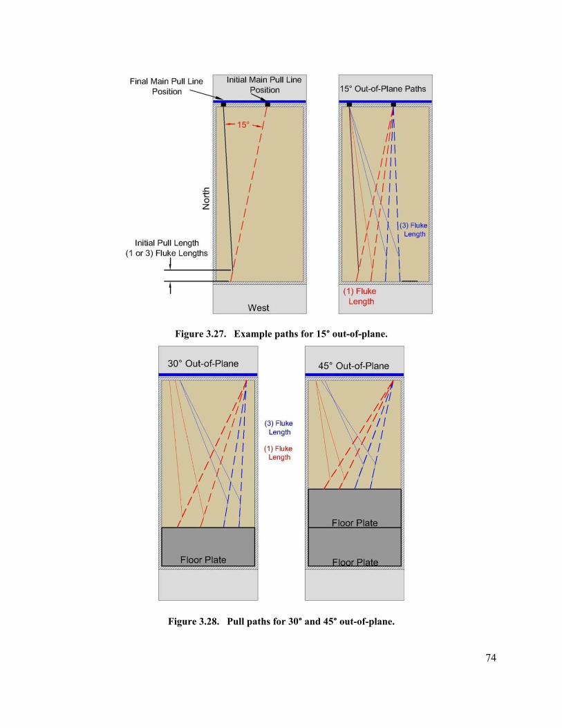
74

Figure 3.27. Example paths for 15° out-of-plane.

Figure 3.28. Pull paths for 30° and 45° out-of-plane.

75

Table 3.4. Case 2 out-of-plane offset distances.

3.7.3 Case 3. Carriage Ladder Mounted Out-of-Plane Tests

These out of plane tests involved mounting the anchor angle apparatus directly to the

lower carriage ladder frame. The vertical anchor angle zero position remained the same, however

the horizontal zero position was changed to 45° off the sediment pit’s x-axis directed to the

north. This was to accommodate the potentially large range of angular displacement. The main

pull cable was reduced in length to approximately 2 ft before connecting to the original chain

with a length of 34 inches. The anchor instrumentation remained as previous. The chaser angle

apparatus was move to the east end of the pit and functioned in the same manner as the previous

tests. The anchor was placed on the surface in the same way as the in-plane tests but oriented

Test #

Offset 

Angle (°)

Fluke 

Angle (°)

First Displacment 

(Fluke lengths)

Anchor dist. from 

north wall (ft)

First Pull Line dist. 

from north wall (ft)

Second Pull Line dist. 

from north wall (ft)

82 15 36 1 2 7 1

83 15 36 1 4 7 1

84 15 36 3 6 7 1

85 15 36 3 8 7 1

94 15 50 1 2 7 1

95 15 50 1 4 7 1

96 15 50 3 6 7 1

97 15 50 3 8 7 1

86 30 36 1 2 11 1

87 30 36 1 5 11 1‐'9"

88 30 36 3 8 11 2'‐5"

89 30 36 3 10 11 2'‐5"

98 30 50 1 2 11 1

99 30 50 1 5 11 1‐'9"

100 30 50 3 8 11 2'‐5"

101 30 50 3 10 11 2'‐5"

91 45 36 1 2 11 1

92 45 36 1 4 11 1

93 45 36 3 6 11 2'‐3"

94 45 36 3 8 11 1'‐9"

102 45 50 1 2 11 1

103 45 50 1 4 11 1

104 45 50 3 6 11 2'‐3"

105 45 50 3 8 11 1'‐9"

Add one floor plate

Add 2nd floor plate

Mix Sediment

Mix Sediment

Mix Sediment

76

due south. The carriage’s y-axis velocity was programmed to 0.42 ft/s to match the x axis

velocity. As illustrated in Figure 3.29 the short main pull cable and anchor were position due

south on the eastern most end of the sediment pit attached to the carriage ladder. The ladder

moved south for an initial embedment of 1 or 3 fluke lengths depending on the tests schedule.

Immediately after reaching position 2, the carriage ladder moved west at the fixed rate of 0.42

ft/s for a distance of 15 ft. The ladder path is labeled in blue and the observed approximated

example path of the anchor is represented by the black line. A total of four tests, numbers 145-

148, were conducted.

Figure 3.29. Ladder mounted out-of-plane pull path example

3.8 Dredge/Tow Carriage Operation

The dredge/tow carriage is shown in Figure 3.30 (left) with the sediment (mud) pit on the

right showing the model anchor being lifted out of the mud. A wash tank is shown in the front of

the mud pit that was used to wash off the model anchor after each test. The control console is

shown in Figure 3.31 (left) and was used to control the distance and speed of the tow carriage.

The sediment pit and mud mixer are shown on the right side of Figure 3.31.

77

Figure 3.30. Dredge/tow carriage and sediment pit (left) and model anchor being lifted out of the mud after a test (right).

Figure 3.31. Dredge/tow carriage control console (left) and sediment pit with mud mixer (right).

The data acquisition system was run through a graphical user interface on a standard

personal computer (PC) and was able to access a manual operating station as well as all of the

necessary drives needed to run the Dredge/Tow Carriage. A picture of the manual operating

station alongside the dredge automation PC can be viewed in Figure 3.32. The PC was also able

78

to record data from the installed gauges. The graphical user interface (GUI) was located in the

personal computer (PC), but the control of the carriage could be manually controlled from the

operator station location. In manual or GUI controlled modes, data are relayed to and from the

servo and vector programmable logic computers (PLC). The servo PLC’s control and obtain

data for the tower, cradle, and ladder movements. The vector PLC controls and obtains data for

the movement of the carriage movements. Data for the horizontal position of the carriage along

the tow flume was obtained through the vector PLC using the laser shown in Figure 3.32.

Figure 3.32. Manual control system (left) and PC control system and horizontal position laser

mounted on the dredge/tow carriage (right).

The anchor was attached to the tow line that was then attached to the carriage. Three

directions of motions (along the tank, across the tank and vertical direction) were accomplished

by moving the carriage and the ladder. A graphical user interface program was written in

Lookout Direct, as shown in the Figure 3.33, was used to control both the carriage and the

ladder. Current coordinates were read from the digital meters on the carriage. Before each test,

target positions were set into the GUI program to move the carriage/ladder. The speeds were set

on the three motors controlling the motion in each direction. Among the three speeds, the

carriage speed along the tank can also be varied on the GUI program panel.

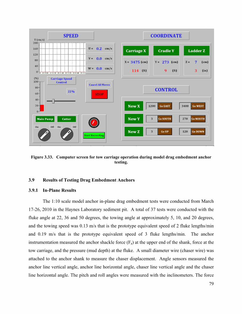
79

Figure 3.33. Computer screen for tow carriage operation during model drag embedment anchor testing.

3.9 Results of Testing Drag Embedment Anchors

3.9.1 In-Plane Results

The 1:10 scale model anchor in-plane drag embedment tests were conducted from March

17-26, 2010 in the Haynes Laboratory sediment pit. A total of 37 tests were conducted with the

fluke angle at 22, 36 and 50 degrees, the towing angle at approximately 5, 10, and 20 degrees,

and the towing speed was 0.13 m/s that is the prototype equivalent speed of 2 fluke lengths/min

and 0.19 m/s that is the prototype equivalent speed of 3 fluke lengths/min. The anchor

instrumentation measured the anchor shackle force (Fa) at the upper end of the shank, force at the

tow carriage, and the pressure (mud depth) at the fluke. A small diameter wire (chaser wire) was

attached to the anchor shank to measure the chaser displacement. Angle sensors measured the

anchor line vertical angle, anchor line horizontal angle, chaser line vertical angle and the chaser

line horizontal angle. The pitch and roll angles were measured with the inclinometers. The force

80

between the tow line and connection to the tow carriage was also measured. The test plan for the

in-plane tests is shown in Table 3.5. Grouping was done in fours based on the fluke angle

setting. A comparison sheet is provided in each workbook with plot overlays showing the

repeated parameters for comparison. The calculated data for the anchor trajectory includes shank

pad eye depth (z) as a function of the horizontal displacement (x) and displacement across the

sediment pit (y) as a function of the horizontal distance along the sediment pit longitudinal axis

(x). The results of all in-plane tests were placed on a CD and attached with this report in

Appendix I.

Table 3.5. Performance of model drag embedment anchor in-plane test plan.

Date Test Fluke angle () deg Initial Tow angle () deg Tow speed (V) m/s 3/17/10 1 36 5 0.13 3/22/10 2 36 5 0.13 3/22/10 3 36 5 0.19 3/22/10 4 36 5 0.13 3/22/10 5 36 5 0.19 3/23/10 6 22 5 0.13 3/23/10 7 22 5 0.19 3/23/10 8 22 5 0.13 3/23/10 9 22 5 0.19 3/24/10 10 50 5 0.13 3/24/10 11 50 5 0.19 3/24/10 12 50 5 0.13 3/24/10 13 50 5 0.19 3/24/10 14 50 10 0.13 3/24/10 15 50 10 0.19 3/24/10 16 50 10 0.13 3/24/10 17 50 10 0.19 3/25/10 18 36 10 0.13 3/25/10 19 36 10 0.19 3/25/10 20 36 10 0.13 3/25/10 21 36 10 0.19 3/25/10 22 22 10 0.13 3/25/10 23 22 10 0.19 3/25/10 24 22 10 0.13 3/25/10 25 22 10 0.19 3/25/10 26 22 20 0.13 3/25/10 27 22 20 0.19 3/26/10 28 22 20 0.13 3/26/10 29 22 20 0.19 3/26/10 30 36 20 0.13 3/26/10 31 36 20 0.19 3/26/10 32 36 20 0.13 3/26/10 33 36 20 0.19 3/26/10 34 50 20 0.13 3/26/10 35 50 20 0.19 3/26/10 36 50 20 0.13 3/26/10 37 50 20 0.19

Examples of the results for test 10 are shown in Figure 3.34 and Figure 3.35. For this test

the fluke angle was 50 degrees, the initial tow angle was approximately 5 degrees, and the tow

81

speed was 0.13 m/s. The pressure transducer data show the anchor continued to penetrate the

sediment to a depth of 4 ft at 40 seconds. The anchor was pulled at a speed of 0.13 m/s over a

distance of 16 ft. The anchor was initially placed in the sediment with the shank parallel to the

top of the sediment and the fluke submerged in the mud at the 50o fluke angle. The force

measured at the fluke pad eye increased to a maximum value of 70 lb at 40 s. The inclinometer

measurements show the anchor rolled less than 10 degrees. The pitch angle decrease from

approximately 36o to zero degrees at 40 s. The anchor and chaser angle sensors show the anchor

pulled straight across the sediment pit. The pad eye depth trajectory was computed from the

chaser displacement, geometry of the support pulleys, and chaser angle measurements. The

results show the pad eye reached a depth of 2 ft at the end of the pull, or 40 s.

The in-plane test 13 was the same as test 10 except the pull speed was increased to 0.19

m/s. Figure 3.36 and Figure 3.37 show the results for this test. The pressure sensor indicates the

anchor penetrated to 3.8 ft which is lightly less than that found in test 10. The anchor force was

the same at 70 lb at the end of the pull (28 s). The pad eye penetration reached approximately 2

ft. The inclinometer measurements for roll showed the anchor roll reached 18o which was

double that of the 0.13 m/s pull. The pitch angle flattened to zero degrees as was measured in

test 10. The anchor again pulled very straight as shown by the angle sensors.

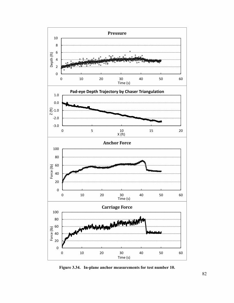
82

Figure 3.34. In-plane anchor measurements for test number 10.

0

2

4

6

8

10

0 10 20 30 40 50 60

Dep

th (ft)

Time (s)

Pressure

‐3.0

‐2.0

‐1.0

0.0

1.0

0 5 10 15 20

Z (ft)

X (ft)

Pad‐eye Depth Trajectory by Chaser Triangulation

0

20

40

60

80

100

0 10 20 30 40 50 60

Force (lb)

Time (s)

AnchorForce

0

20

40

60

80

100

0 10 20 30 40 50 60

Force (lb)

Time (s)

CarriageForce

83

Figure 3.35. In-plane measurements for chaser, anchor, displacement, and pitch and roll for test 10.

0

5

10

15

20

25

30

0 10 20 30 40 50 60

Displacemen

t (ft)

Time (s)

ChaserDisplacement

‐60

‐40

‐20

0

20

40

60

0 10 20 30 40 50 60

Angle (°)

Time (s)

Inclinometer

Inclinometer RollInclinometer Pitch

0

10

20

30

40

0 10 20 30 40 50 60

Angle (°)

Time (s)

AnchorAngle

Anchor Angle HAnchor Angle V

0

60

120

180

240

300

360

0 10 20 30 40 50 60

Angle (°)

Time (s)

ChaserAngle

Chaser Angle H

Chaser Angle V

84

Figure 3.36. In-plane anchor measurements for test 13.

0

2

4

6

8

10

0 10 20 30 40 50 60

Dep

th (ft)

Time (s)

Pressure

‐4.5

‐3.5

‐2.5

‐1.5

‐0.5

0 5 10 15 20

Z (ft)

X (ft)

Pad‐eye Depth Trajectory by Chaser Triangulation

0

20

40

60

80

100

0 10 20 30 40 50 60

Force (lb)

Time (s)

AnchorForce

0

20

40

60

80

100

0 10 20 30 40 50 60

Force (lb)

Time (s)

CarriageForce

85

Figure 3.37. In-plane angle measurements for test 13.

0

5

10

15

20

25

30

0 10 20 30 40 50 60Displacemen

t (ft)

Time (s)

ChaserDisplacement

‐60

‐40

‐20

0

20

40

60

0 10 20 30 40 50 60

Angle (°)

Time (s)

Inclinometer

Inclinometer Roll

Inclinometer Pitch

0

5

10

15

20

0 10 20 30 40 50 60

Angle (°)

Time (s)

AnchorAngle

Anchor Angle H

Anchor Angle V

0

60

120

180

240

300

360

0 10 20 30 40 50 60

Angle (°)

Time (s)

ChaserAngle

Chaser Angle HChaser Angle V

86

The calculated trajectory was measured using spherical coordinates with the origin

starting at the chaser line lower pulley edge from which the line exits. The assumption used was

treating the chaser cable as a straight line. The initial positions for Xo,Yo,Zo and chaser line

length from pulley to anchor (r) was determined by using the constant height of 2.7 ft from the

mud line to chaser pulley apparatus and the initial vertical and horizontal chaser line angles. The

origin was then transformed to the anchor’s starting position at the mud line by subtracting Xo,

Yo, Zo and r. A six location strength profile was obtained on 3/25/2010 (reference T-bar excel

file 0325) as shown in Figure 3.38.

Figure 3.38. Six locations sediment strength profile for March 25, 2010.

Figure 3.39 is a comparison of test number 10 (50° fluke angle, 5° tow angle, 0.13 m/s

tow speed) and test 13 which is a duplicate, however towed at the faster 0.19 m/s speed. The

scatter in the pressure data is consistent throughout all of the tests. It is important to note that the

pressure reading was from the fluke plate and has not been transformed to the shackle pad eye.

The chaser displacement was used for identifying the start and end of the runs, and the slope was

used for verifying the towing speed. The carriage force was consistently noisy with minor

oscillations that were attributed to the vibration observed in the long horizontal span of the main

pull line wire rope from the upper support frame pulley to the carriage connection point.

87

Figure 3.39. Test 10 (0.42ft/s) and test 13 (0.62 ft/s) in-plane 50° sample results.

88

The Z and Y trajectory curves show reasonable agreement and differ by approximately 6

inches by the end of the respective run. The Y variation was thought to be attributed to a slight

misalignment of the anchor initial placement to the anchor towline apparatus position across the

tank (not exactly perpendicular). The variation in the depth and anchor force (not attributed to

tow speed) may be caused by the sediment strength distribution across the tank, since the tests

were not repeated in the exact same location (or lane) in the tank.

Further comparison of in-plane test data is shown in Figure 3.40. Test number 10 with a

50° fluke angle is compared with test 2 with a 36° fluke angle with a tow speed of 0.13 m/s and

initial tow angle of 5°. The resolution of the measuring system clearly records the change of the

anchors response to fluke angle setting. The inclinometer pitch, pressure, and depth trajectory

are appropriate examples. The 22° fluke angle was not used for comparison due to the observed

inability to embed well with the current chain and data cable configuration.

89

Figure 3.40. In-Plane 0.42 ft/s Test 10 (50°) and Test 2 (36°).

The effect of towing angle, tow speed, and fluke angle on the anchor force measured at

the shank pad eye are summarized in Figure 3.41 for the 37 in-plane tests. These results show

the tow angle didn’t have a significant effect on the magnitude of the force. Generally, the tow

speed increase from 0.13 m/s to 0.19 m/s resulted in a small increase in force of 1 to 8 lbs. The

largest effect on the force was due to the fluke angles that were set at 22, 36, and 50 degrees. The

force was measured between 36 and 46 lb for the 22o fluke angle. The force increased to

between 49 and 60 lb for the 36o fluke angle. The largest force was measured for the 50o fluke

angle and the forces were between 60 and 70 lb.

90

The penetration depth as measured by the pressure sensor and the effect of the towing

angle, tow speed, and fluke angle are shown in Figure 3.42. The major effect on penetration

depth was the fluke angle with the larger fluke angle resulting in the largest penetration depth.

For the 50o shank angle the penetration depth reached as deep as 4 ft, and the variation for the

50o fluke angle was 3.0 to 4.1 ft. The penetration depth decreased to between 3.5 and 2.2 ft for

the 36o fluke angle. For the 22o fluke angle, the penetration depth was very close to 2 ft with a

range of between 2.1 and 1.9 ft. As previously found for the force measurements, the effect of

tow speed was very small as shown by the linear trend lines where the dashed line is 0.13 m/s

tow speed and the solid line is 0.19 m/s. As the tow angle increased, the penetration depth tended

to decrease by approximately 2 ft except for the 50o fluke angle at the higher tow speed.

Figure 3.41. Effect of towing angle, tow speed, and fluke angle on the force measured at the shank pad eye and the towing line.

0

10

20

30

40

50

60

70

80

0 5 10 15 20 25

Anchor Force (lb)

Towing Angle (deg)

22 deg, 0.13 m/s

36 deg, 0.13 m/s

50 deg, 0.13 m/s

22 deg, 0.19 m/s

36 deg, 0.19 m/s

50 deg, 0.19 m/s

Linear (22 deg, 0.13 m/s)

Linear (36 deg, 0.13 m/s)

Linear (50 deg, 0.13 m/s)

Linear (22 deg, 0.19 m/s)

Linear (36 deg, 0.19 m/s)

Linear (50 deg, 0.19 m/s)

91

.Figure 3.42. Effect of tow angle, fluke angle, and tow speed on anchor penetration depth as measured by pressure sensor mounted on bottom of model anchor fluke.

3.9.2 Out-of-Plane Results

The 1:10 scale model anchor out-of-plane drag embedment tests were conducted from

March 30-May 2, 2010 in the Haynes Laboratory sediment pit. A total of 68 tests were

conducted with the fluke angle at 22, 36 and 50 degrees, the towing angle at approximately 5, 10,

and 20 degrees, and the towing speed was 0.13 m/s that is the prototype equivalent speed of 2

fluke lengths/min and 0.19 m/s that is the prototype equivalent speed of 3 fluke lengths/min. The

anchor instrumentation measured the force (Fa) at the upper end of the shank, chaser depth at the

upper end of the fluke, and the pressure (mud depth) at the fluke. The pitch and roll angles were

measured with two inclinometers and chaser line angles were measured with angle sensors. The

force between the tow line and connection to the tow carriage was also measured. The test plan

for the in-plane tests is shown in Table 3.6. The data, results, videos and pictures of all the out-

of-plane tests were placed on a CD and attached with this report in Appendix I.

0

0.5

1

1.5

2

2.5

3

3.5

4

4.5

0 5 10 15 20 25

Penetration Depth (ft)

Towing Angle (deg)

 22 deg, 0.13 m/s

 36 deg, 0.13 m/s

 50 deg, 0.13 m/s

22 deg, 0.19 m/s

36 deg, 0.19 m/s

50 deg, 0.19 m/s

Linear ( 22 deg, 0.13 m/s)

Linear ( 36 deg, 0.13 m/s)

Linear ( 50 deg, 0.13 m/s)

Linear (22 deg, 0.19 m/s)

Linear (36 deg, 0.19 m/s)

Linear (50 deg, 0.19 m/s)

92

Table 3.6. Model drag embedment anchor out-of-plane test plan.

Date Test Fluke angle () deg

Tow angle () deg

Tow speed (V) m/s

Out of plane angle () deg

Comments

3/30/10 42 36 5 0.13 45 3/30/10 43 36 5 0.19 45 3/30/10 44 36 5 0.13 45 3/30/10 45 36 5 0.19 45 3/31/10 46 22 5 0.13 45 3/31/10 47 22 5 0.19 45 3/31/10 48 22 5 0.13 45 3/31/10 49 22 5 0.19 45 3/31/10 50 50 5 0.13 45 3/31/10 51 50 5 0.19 45 3/31/10 52 50 5 0.13 45 3/31/10 53 50 5 0.19 45 3/31/10 54 50 5 0.13 90 3/31/10 55 50 5 0.19 90 3/31/10 56 50 5 0.13 90 3/31/10 57 50 5 0.19 90 3/31/10 58 36 5 0.13 90 3/31/10 59 36 5 0.19 90 3/31/10 60 36 5 0.13 90 3/31/10 61 36 5 0.19 90 3/31/10 62 22 5 0.13 90 3/31/10 63 22 5 0.19 90 4/1/10 64 22 5 0.13 90 4/1/10 65 22 5 0.19 90 4/1/10 66 50 5 0.13 90 imbed 4/2/10 67 50 5 0.19 90 imbed 4/2/10 68 50 5 0.13 90 imbed 4/2/10 69 50 5 0.19 90 imbed 4/2/10 70 50 5 0.13 45 imbed 4/2/10 71 50 5 0.19 45 imbed 4/2/10 72 50 5 0.13 45 imbed 4/2/10 73 50 5 0.19 45 imbed 4/7/10 74 36 5 0.13 90 imbed 4/7/10 75 36 5 0.19 90 imbed 4/7/10 76 36 5 0.13 90 imbed 4/7/10 77 36 5 0.19 90 imbed 4/7/10 78 36 5 0.13 45 imbed 4/7/10 79 36 5 0.19 45 imbed 4/7/10 80 36 5 0.13 45 imbed 4/7/10 81 36 5 0.19 45 imbed 4/8/10 82 36 5 0.13 15 Imbed 1 fluke length initial pull, then pull at out of plane angle 4/8/10 83 36 5 0.13 15 Imbed 1 fluke length initial pull, then pull at out of plane angle 4/8/10 84 36 5 0.13 15 Imbed 3 fluke length initial pull, then pull at out of plane angle 4/8/10 85 36 5 0.13 15 Imbed 3 fluke length initial pull, then pull at out of plane angle 4/9/10 86 36 5 0.13 30 Imbed 1 fluke length initial pull, then pull at out of plane angle 4/9/10 87 36 5 0.13 30 Imbed 1 fluke length initial pull, then pull at out of plane angle 4/9/10 88 36 5 0.13 30 Imbed 3 fluke length initial pull, then pull at out of plane angle 4/9/10 89 36 5 0.13 30 Imbed 3 fluke length initial pull, then pull at out of plane angle 4/8/10 90 36 5 0.13 45 Imbed 3 fluke length initial pull, then pull at out of plane angle 4/8/10 91 36 5 0.13 45 Imbed 3 fluke length initial pull, then pull at out of plane angle 4/8/10 92 36 5 0.13 45 Imbed 3 fluke length initial pull, then pull at out of plane angle 4/8/10 93 36 5 0.13 45 Imbed 3 fluke length initial pull, then pull at out of plane angle 4/8/10 94 50 5 0.13 15 Imbed 1 fluke length initial pull, then pull at out of plane angle 4/8/10 95 50 5 0.13 15 Imbed 1 fluke length initial pull, then pull at out of plane angle 4/8/10 96 50 5 0.13 15 Imbed 3 fluke length initial pull, then pull at out of plane angle 4/8/10 97 50 5 0.13 15 Imbed 3 fluke length initial pull, then pull at out of plane angle 4/8/10 98 50 5 0.13 30 Imbed 1 fluke length initial pull, then pull at out of plane angle 4/8/10 99 50 5 0.13 30 Imbed 1 fluke length initial pull, then pull at out of plane angle 4/8/10 100 50 5 0.13 30 Imbed 3 fluke length initial pull, then pull at out of plane angle 4/8/10 101 50 5 0.13 30 Imbed 3 fluke length initial pull, then pull at out of plane angle 4/9/10 102 50 5 0.13 45 Imbed 3 fluke length initial pull, then pull at out of plane angle 4/9/10 103 50 5 0.13 45 Imbed 3 fluke length initial pull, then pull at out of plane angle 4/9/10 104 50 5 0.13 45 Imbed 3 fluke length initial pull, then pull at out of plane angle 4/9/10 105 50 5 0.13 45 Imbed 3 fluke length initial pull, then pull at out of plane angle 5/2/10 145 50 5 0.13 15,30,45 Imbed 1 fluke length initial pull, then pull at out of plane angle 5/2/10 146 50 5 0.13 15, 30, 45 Imbed 1 fluke length initial pull, then pull at out of plane angle 5/2/10 147 50 5 0.13 15,30,45 Imbed 3 fluke length initial pull, then pull at out of plane angle 5/2/10 148 50 5 0.13 15, 30, 45 Imbed 3 fluke length initial pull, then pull at out of plane angle

93

The out of plane measured and calculated data was obtained by using the same methods

as described for the in-plane results. For comparison purpose of test 98 and test 100 as shown in

Figure 3.44 the X-axis for all but the trajectory plots were converted from time to X

displacement in feet. The purpose of the conversion was to clarify and better illustrate the data

during the anchor’s motion. As described previously for out-of-plane procedures, there was a

necessary delay in the test after the initial embedment distance to stop and reposition the running

gear for the new heading. Figure 3.43 is an example of test 98 with a time series axis. The delay

time to reset the gear is shown by the zero slope sections in the chaser displacement plot. For

this test there was approximately a 130 second delay starting at 15 s to 145 s; during the delay

the anchor force shows a considerable drop with modulations attributed to the motion of the

anchor line from one of the operators moving the gear. This section of data should not be

interpreted as data attributed to normal embedment properties. Compare test 98 anchor force

profile from Figure 3.43 to that shown in Figure 3.44 where the delay is collapsed by converting

the time series to x displacement motion and the result is a better visual depiction.

94

Figure 3.43. Example Test 98 Out-of-Plane Data Time Delay

The parameters for test 98 and 100 were 30° out-of-plane heading change, 0.13 m/s tow

speed and a fluke angle of 50°. Test 98 was a 1 fluke length initial embedment distance and test

100 was for 3 fluke lengths. The spikes found in the plots of Figure 3.44 at approximately 1.7 ft

and 3.2 ft correspond to the time delay collapse as described above.

The profiles of the plots in Figure 3.44 show reasonable agreement. The anchor angle H

(horizontal) indicates the heading change after the initial embedment length. For test 98 the

heading angle started at 120° and after resetting the gear, arrived at 153° for an out-of-plane

angle of 33° for a 3° overage of the target 30° anchor line heading. Test 100 however shows a

heading change of nearly 41°, or 11° over the target. This overage may be attributed to the

inconsistent ability to remove the excess slack in the main tow line after resetting the gear.

The reduction of depth shown in the pressure profiles of Figure 3.44 at the 1.7 ft and 3.2

ft locations where the anchor movement was stopped for resetting suggests that the pressure

gauge may be reading a dynamic force in addition to the hydrostatic. This would explain the

95

consistently higher depth readings of the pressure gauge over and above the physical offset of the

pressure gauge location with respect to the shackle depth trajectory.

Figure 3.44. Out-of-Plane Test 98 and 100 Comparisons

96

The test number 100 lower anchor force may also be attributed to the physical location of

the path in the sediment tank and the corresponding variation of soil strength. The 3 fluke length

30° out-of-plane tests were performed in the southwestern section of the tank as shown in Figure

3.28. The soil strength test point corresponding to this location was T-bar test number 3 as

shown in the previous Figure 3.21. The soil strength profile for test point 3 verses test point 6

where test number 98 was performed from Figure 3.38 shows a 1.5 psf lower reading, indicating

that test 100 passed through weaker soil. The differences in the Y trajectories are related to the

predetermined path location for the 1 and 3 fluke length 30° out-of-plane paths as shown in

Figure 3.28. It is apparent that although the anchor line heading change was at least 30° the

anchors heading change was as expected much less.

The out of plane tests 82 through 105 are analyzed to evaluate the effect of the out of

plane pull angle on the maximum increase penetration depth, maximum force at the model

anchor shank pad eye, and the roll angle when the force is maximum. First, the model anchor

was embedded by pulling the anchor one or three fluke lengths and then the model anchor was

pull at the out of plane pull angle of 15o, 30o and 45o. The fluke angle was set at 36o and 50o and

the towing angle between the sediment bed and the tow line was set at 5o. The maximum

penetration increase after the initial embedment was determined. The results of the maximum

increase in the penetration depth are shown in Figure 3.45 for the out of plane pull angles. The

50o fluke penetration increase is 0.4 ft for the out of plane pull angles of 15o and 45o and 0.2 ft

for the 30o angle. The polynomial curve fits to the data indicate a slight increase of 0.2 ft for the

30 out of plane pull angle. Figure 3.46 illustrates the effect of the out of plane pull angle on the

maximum force measured at the shank pad eye. The largest forces for the 50o and 36o fluke

angles were 86 lb and 65 lb for the 15o pull angle, respectively. The forces generally decreased

as the pull angle increased to 30o and 45o. The 50o fluke angle showed a larger force decrease

that the 36 o fluke angle. The roll angle measured by the inclinometers on the bottom of the

anchor fluke are shown in Figure 3.47. The roll angle data show significant scatter, but the

general trend is for the largest roll angle to occur with the 50o fluke angle for the 15o pull angle

and the roll angle generally decreased with increasing pull angle of 30o and 45o. The largest roll

97

angle measured was 20o when pulling at an angle of 15o, but all the other roll angles were

measured between 0 and 10o.

Figure 3.45. Effect out of plane pull angle on maximum penetration increase after initial embedment for the model anchor with 36o and 50o fluke angles.

R² = 0.57

R² = 0.0618

0

0.5

1

1.5

2

2.5

0 10 20 30 40 50

Maxim

um Penetration In

crease after initial embedment (ft of mud)

Out of Plane Angle (degree)

36 degree fluke angle

50 degree fluke angle

Poly. (36 degree fluke angle)

Poly. (50 degree fluke angle)

98

Figure 3.46. Maximum force at the model anchor shank padeye for three out of plane pull angles after initial embedment.

Figure 3.47. Model anchor roll angle as a result of out of plane pull angle.

R² = 0.4438

R² = 0.5693

50

60

70

80

90

100

0 10 20 30 40 50

Maxim

um Force at shan

k pad

eye

 (lb)

Out of Plane Angle (degree)

36 deg fluke angle

50 deg fluke angle

Linear (36 deg flukeangle)

Poly. (50 deg flukeangle)

R² = 0.0425

R² = 0.797

0.0

5.0

10.0

15.0

20.0

25.0

0 10 20 30 40 50

Roll Angle at Maxim

um Force (deg)

Out of Plane Angle (deg)

Roll angle for 36 degfluke angle

Roll angle for 50 degfluke angle

Poly. (Roll angle for 36deg fluke angle)

Poly. (Roll angle for 50deg fluke angle)

99

3.9.3 Break-out Results

The 1:10 scale model anchor in-plane drag embedment tests were conducted from April

20-April 22, 2010 in the Haynes Laboratory sediment pit. A total of 36 tests were conducted

with the fluke angle at 22, 36 and 50 degrees. The test plan for the in-plane tests is shown in

Table 3.7. The results of all breakout tests were placed on a CD and attached with this report in

Appendix I. The break-out results are interpreted in Chapter 4.

Table 3.7. Model drag embedment anchor breakout test plan.

Date Test Fluke angle () deg

Breakout degree of freedom

Comments

4/20/10 109 50 heave Imbed 3 fluke length initial pull, then conduct break out 4/20/10 110 50 Heave Imbed 3 fluke length initial pull, then conduct break out

4/23/10 111 112

50 Pitch Down Imbed 3 fluke length initial pull, then conduct break out

4/23/10 111B 112B

50 Pitch Up Imbed 3 fluke length initial pull, then conduct break out

4/23/10 113 50 roll Imbed 3 fluke length initial pull, then conduct break out 4/23/10 114 50 roll Imbed 3 fluke length initial pull, then conduct break out 4/21/10 115 50 Fwd trans Imbed 3 fluke length initial pull, then conduct break out 4/21/10 116 50 Fwd trans Imbed 3 fluke length initial pull, then conduct break out 4/21/10 117 50 Side trans Imbed 3 fluke length initial pull, then conduct break out 4/21/10 118 50 Side trans Imbed 3 fluke length initial pull, then conduct break out 4/22/10 119 50 Rotation Imbed 3 fluke length initial pull, then conduct break out 4/22/10 120 50 rotation Imbed 3 fluke length initial pull, then conduct break out 4/20/10 121 36 heave Imbed 3 fluke length initial pull, then conduct break out 4/20/10 122 36 heave Imbed 3 fluke length initial pull, then conduct break out

4/23/10 123 124

36 Pitch Down Imbed 3 fluke length initial pull, then conduct break out

4/23/10 123B 124B

36 Pitch Up Imbed 3 fluke length initial pull, then conduct break out

4/23/10 125 36 roll Imbed 3 fluke length initial pull, then conduct break out 4/23/10 126 36 roll Imbed 3 fluke length initial pull, then conduct break out 4/21/10 127 36 Fwd trans Imbed 3 fluke length initial pull, then conduct break out 4/21/10 128 36 Fwd trans Imbed 3 fluke length initial pull, then conduct break out 4/21/10 129 36 Side trans Imbed 3 fluke length initial pull, then conduct break out 4/21/10 130 36 Side trans Imbed 3 fluke length initial pull, then conduct break out 4/22/10 131 36 Rotation Imbed 3 fluke length initial pull, then conduct break out 4/22/10 132 36 rotation Imbed 3 fluke length initial pull, then conduct break out 4/21/10 133 22 heave Imbed 3 fluke length initial pull, then conduct break out 4/21/10 134 22 heave Imbed 3 fluke length initial pull, then conduct break out

4/23/10 135 136

22 Pitch Down Imbed 3 fluke length initial pull, then conduct break out

4/23/10 135B 136B

22 Pitch Up Imbed 3 fluke length initial pull, then conduct break out

4/23/10 137 22 roll Imbed 3 fluke length initial pull, then conduct break out 4/23/10 138 22 roll Imbed 3 fluke length initial pull, then conduct break out 4/21/10 139 22 Fwd trans Imbed 3 fluke length initial pull, then conduct break out 4/21/10 140 22 Fwd trans Imbed 3 fluke length initial pull, then conduct break out 4/21/10 141 22 Side trans Imbed 3 fluke length initial pull, then conduct break out 4/21/10 142 22 Side trans Imbed 3 fluke length initial pull, then conduct break out 4/22/10 143 22 Rotation Imbed 3 fluke length initial pull, then conduct break out 4/22/10 144 22 rotation Imbed 3 fluke length initial pull, then conduct break out

100

3.10 Summary and Conclusions

A 1:10 generic scale model of a drag embedment anchor was tested in the dredge/tow

tank in the Haynes Laboratory at Texas A&M University. Both in-plane and out-of-plane

performance of DEAs were investigated. The dredge/tow tank is 45.6 m (149.5 ft) long 3.66 m

(12 ft) wide, with a maximum water depth of 3.05 m (10 ft). The dredge/tow tank has a sediment

pit that is 7.6 m (25 ft) long, 3.7 m (12 ft) wide, and 1.5 m (5 ft) deep, and the volume of the

sediment pit is 1500 ft3 or 11,200 gallons. The dredge/tow carriage is capable of speeds up to 2

m/s (4 kts) and has a vertical ladder that can move vertically and horizontally. A sand-bentonite-

water mixture was mixed on site and placed in the sediment pit. Procedures were developed and

instrumentation acquired to measure the anchor location (x, y and z) as function of time, fluke

angle (pitch, roll and yaw), line load, and inclination of the anchor as it is towed through the

sediment. The model drag embedment anchor was towed with a cable connected to the

dredge/tow carriage through a bottom mounted pulley support structure. The dredge tow

carriage has speed control and position monitoring instruments with data acquisition.

For test number 10, the fluke angle was 50 degrees, the tow angle was approximately 5

degrees, and the tow speed was 0.13 m/s. The pressure transducer data show the anchor

continued to penetrate the sediment to a depth of 4 ft at 40 seconds. The force measured at the

fluke pad eye increased to a maximum value of 70 lb at 40 s. The anchor rolled less than 10

degrees, and the pitch angle decrease from approximately 36o to zero degrees at 40 s. The pad

eye depth trajectory computed from the chaser displacement, geometry of the support pulleys,

and chaser angle measurements shows the pad eye reached a depth of 2 ft at the end of the pull,

or 40 s. The Z and Y trajectory curves show reasonable agreement and differ by approximately 6

inches by the end of the respective run. The Y variation was attributed to a slight misalignment

of the anchor initial placement to the anchor towline apparatus position across the tank (not

exactly perpendicular). The variation in the depth and anchor force (not attributed to tow speed)

may be caused by the sediment strength distribution across the tank, since the tests were not

repeated in the exact same location (or lane) in the tank.

The in-plane results show the tow angle didn’t have a significant effect on the magnitude

of the force. Generally, the tow speed increase from 0.13 m/s to 0.19 m/s resulted in a small

101

increase in force of 1 to 8 lbs. The largest effect on the force was due to the fluke angles that

were set at 22, 36, and 50 degrees. The force was measured between 36 and 46 lb for the 22o

fluke angle. The force increased to between 49 and 60 lb for the 36o angle. The largest force

was measured for the 50o fluke angle and the forces were between 60 and 70 lb.

The major effect on penetration depth was the fluke angle with the larger fluke angle

resulting in the largest penetration depth. For the 50o shank angle the penetration depth reached

as deep as 4 ft, and the variation for the 50o fluke angle was 3.0 to 4.1 ft. The penetration depth

decreased to between 3.5 and 2.2 ft for the 36o fluke angle. For the 22o fluke angle, the

penetration depth was very close to 2 ft with a range of between 2.1 and 1.9 ft. As the tow angle

increased, the penetration depth tended to decrease by approximately 2 ft except for the 50o fluke

angle at the higher tow speed.

For out-of-plane test number 98 the heading angle started at 120° and after resetting the

gear, arrived at 153° for an out-of-plane angle of 33° for a 3° overage of the target 30° anchor

line heading. Test 100 however shows a heading change of nearly 41°, or 11° over the target.

This overage may be attributed to the inconsistent ability to remove the excess slack in the main

tow line after resetting the gear.

The reduction of depth shown in the pressure profiles at the 1.7 ft and 3.2 ft locations

where the anchor movement was stopped for resetting suggests that the pressure gauge may be

reading a dynamic force in addition to the hydrostatic. This would explain the consistently

higher depth readings of the pressure gauge over and above the physical offset of the pressure

gauge location with respect to the shackle depth trajectory.

The test 100 lower anchor force may also be attributed to the physical location of the path

in the sediment tank and the corresponding variation of soil strength. The 3 fluke length 30° out-

of-plane tests were performed in the southwestern section of the tank. The soil strength profile

for test point 3 vs. test point 6 (where Test 98 was performed) shows a 1.5 psf lower reading,

indicating that test 100 passed through weaker soil. The differences in the Y trajectories are

related to the predetermined path location for the 1 and 3 fluke length 30° out-of-plane paths. It

102

is apparent that although the anchor line heading change was at least 30° the anchors heading

change was much less.

The out of plane tests generally showed the 50o fluke angle produced a larger maximum

increase in penetration depth, a higher force at the shank pad eye, and larger roll angles that

those measured for the 36o fluke angle. The maximum increase in penetration depth was slightly

larger by 0.2 ft for the 30o pull angle than that measured for the 15o and 45o pull angles. The

maximum force at the shank pad eye generally showed a decrease as the pull angle increased

from 15o to 45o, and the 50 fluke angle had larger values of force that those measured with the 36

fluke angle. The out of plane roll angle data showed significant scatter, but on the average the

50o fluke angle showed larger roll angles than the 36o. The roll angles decreased slightly and the

out of plane pull angle increased from 15o to 45o.

103

4.0 Model Development and Evaluation

This section presents theoretical formulations for in-plane and out-of-plane drag embedment

anchor behavior (Figure 4.1), and evaluates the models in light of the experimental data

generated in this research.

4.1 In-Plane Behavior

Two aspects of drag anchor performance must be considered when formulating a predictive

model for drag embedment: load capacity and trajectory, the trajectory being the embedment

depth versus drag distance. The discussion below will show that these two aspects of behavior

are in fact inter-related. Load capacity generally increases with anchor embedment depth.

However, the depth to which a drag anchor will penetrate depends on the load resistance

characteristics of the anchor. For this reason, the two aspects of behavior must be considered in a

single unified model.

4.1.1 Load Capacity

4.1.1.1 Theoretical Considerations

At a given embedment depth the load capacity Ta (Figure 4.2) of a drag anchor can be expressed

in terms of a bearing factor Ne, the soil undrained shear strength su, and the fluke area Af.

Ta = Ne su Af (Eq. 4.1)

Aubeny and Chi (2010) discuss how Ne is governed by a complex interaction of

combined loads acting on the anchor fluke that involve soil resistance forces acting normal and

parallel (tangential) to the fluke, and a soil resisting moment also acting on the fluke. In general,

Ne will depend on the relative magnitudes of these forces and moments. However, Aubeny and

Chi (2010a) show that during drag embedment anchor rotations, and therefore soil resisting

moments are negligible. Further, the dominant “collapse mechanism” involves translation of the

anchor parallel to the fluke. A normal force does act on the anchor fluke, which will tend to

reduce tangential soil resistance force parallel to the fluke (Eq. 4.2):

Ft = Ntmax su Af (Eq. 4.2)

104

za= Shackle depth

a

Shackle(pad-eye)

Mudline

Anchor Line,b = diameter

x

z

o

f

FlukeArea = Af

Shank

Mudline Tension, T0

Figure 4.1. Definition Sketch of Anchor and Anchor Line System

4.1.1.2 Experimental Evaluation

The definition sketch in Figure 4.2 defines the variables used in the large-scale drag embedment

test interpretation calculations. The anchor bearing factor during drag embedment Ne was

computed by the two methods described in the following paragraphs.

a

Ta = Ne su Af

f Fs = Nsmax su Af

Constant during drag embedment:‐Equilibrium Bearing Factor, Ne

‐Anchor line‐fluke angle:af = a + f

W'

Figure 4.2. Definition Sketch of Force System on Anchor

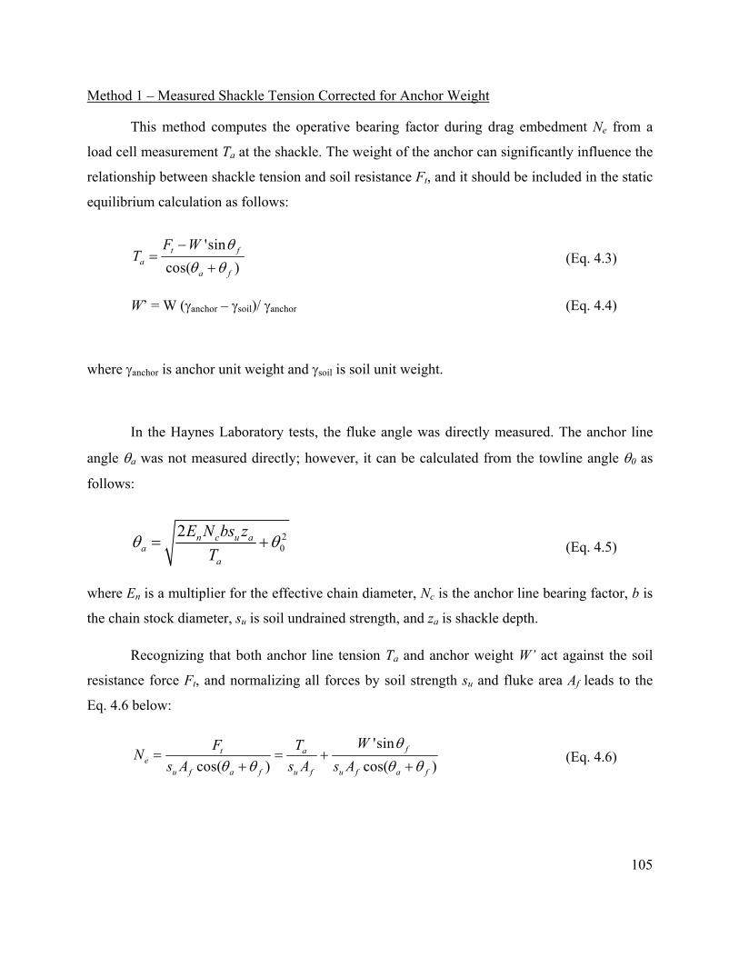
105

Method 1 – Measured Shackle Tension Corrected for Anchor Weight

This method computes the operative bearing factor during drag embedment Ne from a

load cell measurement Ta at the shackle. The weight of the anchor can significantly influence the

relationship between shackle tension and soil resistance Ft, and it should be included in the static

equilibrium calculation as follows:

'sin

cos( )t f

aa f

F WT

(Eq. 4.3)

W’ = W (anchor – soil)/ anchor (Eq. 4.4)

where anchor is anchor unit weight and soil is soil unit weight.

In the Haynes Laboratory tests, the fluke angle was directly measured. The anchor line

angle a was not measured directly; however, it can be calculated from the towline angle 0 as

follows:

20

2 n c u aa

a

E N bs z

T (Eq. 4.5)

where En is a multiplier for the effective chain diameter, Nc is the anchor line bearing factor, b is

the chain stock diameter, su is soil undrained strength, and za is shackle depth.

Recognizing that both anchor line tension Ta and anchor weight W’ act against the soil

resistance force Ft, and normalizing all forces by soil strength su and fluke area Af leads to the

Eq. 4.6 below:

'sin

cos( ) cos( )ft a

eu f a f u f u f a f

WF TN

s A s A s A

(Eq. 4.6)

106

Method 2 – Measured Angle Data with Breakout Test Data

By an alternative procedure, Ne can be computed based on the tangential soil resistance,

the measured pitch angle f and the anchor line angle at the shackle a computed as described

above. In this procedure the following Eq. 4.7 applies:

Ne = Ntmax /cos(f + a) (Eq. 4.7)

The bearing factor for loading of the anchor parallel to the fluke Ntmax was measured in the

breakout tests described earlier.

Example Comparisons of Embedment Bearing Factor Estimates

Data interpretations for Haynes Laboratory Tests 10 and 13 (both 50-degree anchor fluke-

shank angles) are shown in Figure 4.3, where “Series 1” and “Series 2” correspond to Methods 1

and 2, respectively. The bearing factors calculated by the two methods tend to agree during the

early stages of drag embedment as well as at large (>15 ft) drag distances. The maximum

discrepancy between the two methods tends to occur at intermediate drag distances, on the order

of 10 ft. A plausible source of the differences could be that the actual anchor line angle a differs

from that assumed in the calculations. These differences notwithstanding, the general agreement

between the estimates of Ne obtained by essentially independent methods suggests that the data

sets can be used with confidence.

It should be noted that Method 2 relies entirely on a computed estimate of the anchor line

shackle angle a. By contrast, Method 1 relies on a only for the weight correction to the load

cell measurement Ta, which diminishes in significance as the fluke rotates towards f = 0.

Accordingly, when the two methods give conflicting results, greater weight should be given to

Method 1.

107

Figure 4.3. Measured Anchor Bearing Factors, Large-Scale Anchor

with 50-degree Fluke-Shank Angle

108

4.1.1.3 Comparisons between Test Beds

The example analyses summarized in Figure 4.3 were based on 1:10 scale model test data

from Haynes Laboratory, which were performed in a sand-bentonite test bed. The parallel small

(1:30) scale tests were conducted in a kaolinite test bed. In addition, the 1:30 scale tests used a

model anchor that satisfied similitude in all respects with regard to 1:10 scale anchor except one:

the relative thickness of the fluke for the 1:30 scale tests was twice that for the 1:10 scale test.

This deviation from full similitude was unavoidable. The 1:30 scale model anchor (plastic) fluke

could not have been made significantly thinner without introducing excessive flexibility into the

anchor. By contrast, doubling the thickness of the 1:10 scale anchor would have doubled the

anchor weight; conceivably such a heavy anchor could self-penetrate into the mud, which would

invalidate the entire test. Table 4.1 summarizes the major differences between the 1:10 scale and

the 1:30 scale model tests.

Table 4.1. Significant Features of Large and Small Scale Laboratory Model Tests

Feature 1:10 Scale Model

1:30 Scale Model Tests

Drag Embedment Tests in Metal Tank

Pure Loading Test and Drag Embedment

Tests with the Magnetometer

Soil Type Sand-bentonite Kaolinite Kaolinite

Undrained Shear Strength ConstantLinearly Increasing

with depth. Constant

Soil Sensitivity Remolded,

1-1.2 1.5 to 2 Remolded, 1Length of fluke to thickness of fluke (Lf/tf) 60 30 30

Wire line diameter ratio (Af/b2) 150

1300 (thick line) and 21,000 (thin line)

1300 (thick line) and 21,000 (thin line)

Unit Weight of Anchor (pounds per cubic foot) 490 70 70

Observed Rolling During test yes, moderate yes, moderate yes, moderate

Recognizing these differences, Table 4.2 presents a summary comparison of bearing

factors from the large and 1:30 scale tests. The comparisons are presented for the original 1:30

109

scale anchor. Values reported in Table 4.2 correspond to ultimate (large-drag distance)

conditions and bearing factors were computed using Method 1 described above.

Observations from Table 4.2 include the following:

The 1:10 scale tests indicate that a larger fluke-shank angle leads to higher

capacity, in this case the higher fluke-shank angle setting produced an increase in anchor

capacity that exceeded 25%.

The pure shear bearing factors for the original 1:30 scale model anchor exceeded

that of the 1:10 scale model anchor. This difference can largely be attributed to the larger

relative thickness of the fluke in the 1:30 scale model tests.

The equilibrium bearing factor during drag for the 1:30 scale anchor model with a

50-degree fluke-shank angle was about 6 with an associated equilibrium line-fluke angle

of about 45 degrees. In comparison, the equilibrium bearing factor during drag for the

1:10 scale anchor model with a 50-degree fluke-shank angle was about 4 with an

associated equilibrium line-fluke angle of about 55 degrees. These results are consistent

with the different geometries for the two model anchors. The 1:30 scale anchor has a

thicker fluke, a larger resistance to pure shear, a larger resistance to drag once the

equilibrium condition is reached and therefore a flatter equilibrium angle between the line

and the fluke during drag. The 1:10 scale anchor has a thinner fluke, a smaller resistance

to pure shear, a smaller resistance to drag once the equilibrium condition is reached and

therefore a steeper equilibrium angle between the line and the fluke during drag.

Both the 1:30 and the 1:10 scale model anchor experienced some rolling during

in-plane drag embedment tests, but generally it was less than about 20 degrees and did not

seem to affect the trajectory or the line load.

110

Table 4.2. Comparison of Large and Small Scale In-Plane Test Results

Test Type Undrained Shear Strength, su (psf)

Fluke Width

Fluke-Shank Angle (degrees)

Pure Normal Bearing Factor Nnmax

Pure Shear Bearing Factor Ntmax

Bearing FactorNe During Drag

1:10 scale 16-20 Original 36 11.2-11.6 2.1 3.19

Original 50 11-11.6 2.6 4.070.56

1:30 scale 10-12 for pure loading; 8-10 psf/ft for In-plane drag embedment

Wide 50 10.580.09 4.20.01 5.80.921

6.580.332

1Thick loading line. 2Thin loading line.

4.1.2 Anchor Line Behavior

Neubecker and Randolph (1995) also provide equations for the anchor line geometry in

the soil column for two limiting strength profiles: uniform strength (k=0) and strength

proportionate to depth (su0 = 0). Typically, even normally consolidated soil deposits have a non-

zero strength intercept with strength increasing with depth; therefore, an anchor line equation

that describes a range of strength profiles intermediate between the limiting cases derived by

Neubecker and Randolph is desirable. Re-visiting the development of the Neubecker-Randolph

equations showed that the following closed-form solution (Eq. 4.8) for anchor line geometry in

the soil column is applicable to the general case of a linear strength profile with non-zero values

of strength intercept su0 and gradient k.

2 22 1 2 1 2 2 0

2 2 22 2 1 2 1 2 2 0

/ 2 / 21* ln

2 * / 2 ( *) * / 2

Q Q Q Q Q Qx

Q Q z Q Q z Q Q z Q

(Eq. 4.8)

where x* = normalized horizontal coordinate = x/za

z* = normalized vertical coordinate = z/za

111

Q1 = normalized soil resistance due to mudline strength = En Nc b su0 za /Ta

Q2 = normalized soil resistance due to strength gradient = En Nc b k 2az /2Ta

za = depth of pad-eye

su0 = soil strength at mudline

k = soil strength gradient

En = area multiplier for chains

Nc = bearing factor for anchor line

b = anchor line diameter

Ta = anchor line tension at pad-eye

0 = anchor line angle at mudline

For the special limiting case of strength being proportionate to depth (su0 = 0), Q1 is zero

and Eq. 4.8 can be shown to be equivalent to the solution given by Neubecker and Randolph

(1995). Similarly, for the case of a uniform strength profile Q2 is zero, and invoking L’Hopital’s

rule to Eq. 4.8 leads to the other special case derived by Neubecker and Randolph for a uniform

strength profile.

Previous solutions existed only for the special cases of a perfectly uniform strength

profile and a linearly varying strength profile with zero mudline strength. These solutions were

fairly restrictive, since real strength profiles are typically intermediate between these limiting

cases. Figure 4.3 shows anchor line configurations for general strength conditions. The expanded

solutions are very useful in predicting the length of anchor line that will be embedded in the soil

during drag embedment, which in turn affects the solution for the catenary line in the water

column. The improved solution for anchor line configuration has been incorporated as a

subroutine into the anchor trajectory prediction model.

Trajectory and load predictions from the improved analytical predictive model were

utilized to guide the planning and development of the anchor model test program in the Haynes

Laboratory test bed.

112

0

0.2

0.4

0.6

0.8

10 5 10 15 20

z-co

ordi

nate

, z/ z

a

x-coordinate, x/ za

30

* = 100

10

3

T* = 20

0 = 0 degrees

Figure 4.3. Anchor Line Geometry for Various Soil Strength Profiles; the soil strength parameter *= kz/su0, where k=strength gradient, z=pad-eye depth, su0=mudline undrained shear strength

4.1.3 Trajectory during Drag Embedment

Since anchor pullout capacity is proportional to soil strength (Eq. 4.1) and since soil strength

generally increases with depth, realistic prediction of anchor embedment depth, or anchor

trajectory, is an essential component of an overall anchor pullout capacity model. The discussion

below centers on a predictive model for drag embedment trajectory and the experimental

evaluation of the model.

4.1.3.1 Theoretical Considerations

Based on the anchor line equations developed by Neubecker and Randolph (1995) and the

kinematic characteristics of a drag anchor, Aubeny and Chi (2010) present a model for drag

anchor trajectory based on the equation below:

2 2

0

0

0

ˆ ˆ2(1 / )

ˆ

n c a

a a

a

a

E N

d T z

ddz

d

(Eq. 4.9)

where z = normalized depth of shackle = z/b

113

ˆa

T = normalized tension at shackle = Ta / Sua b2 = Neq Af / b

2

b = anchor line diameter Sua = soil shear strength at the shackle

a = anchor line angle at the shackle

0 = anchor line angle at the mudline

= strength gradient parameter = bk/ su0 su0 = soil shear strength at mudline Nc = bearing factor for anchor line En = multiplier for anchor lines comprised of chains k = soil shear strength increase per unit increase in depth

Eq. 4.9 is a recursive equation describing how the anchor line angle at the shackle a

(Figure 4.2) changes as embedment progresses. After an initial transient stage of embedment,

theoretical considerations indicate that the fluke angle f (Figure 4.2) changes at the rate df/dt =

da /dt. From Figure 4.2, it is evident that f will eventually approach horizontal, such that no

further embedment is possible. Thus, Eq. 4.9 provides a means of both predicting embedment as

a function of drag distance, as well as predicting the ultimate possible embedment depth of the

anchor.

Both theory and observation indicate that the angle between anchor line and the anchor

fluke (af =a+f, Figure 4.2) tends toward a constant equilibrium value. This behavior leads to

the relatively simple model of drag anchor trajectory described by Eq. 4.9. However,

experimental evidence (see Figure 4.3 Series 2 data based on Eq. 4.7) indicates that a state of

constant af does not establish itself immediately, but requires some minimal drag distance for

this equilibrium condition to develop. The experiments presented herein provided quantitative

data on the duration of this transient stage.

4.1.3.2 Experimental Evaluation

Anchor trajectory from the large-scale model tests was tracked by the two methods described

below.

114

Method 1 – From Chaser Measurements

With this method, a thin chaser line was attached to the anchor shackle. Continuous

measurements of the chaser line length and inclination angle provided a basis for tracking the

shackle throughout drag embedment. Additionally, inclinometer measurements of pitch (f)

permit tracking of any point on the anchor, most importantly the location of the pressure sensor

on the fluke, which is the basis for Method 2.

Method 2 – From Pressure Sensor Data

A pressure sensor mounted to the fluke provided a second basis for tracking embedment

depth. In a static situation, the pressure sensor can provide depth measurements based on a

simple hydrostatic principle. However, when the anchor is moving the shearing resistance of the

soil will exert an additional component of resistance. The sensor depth estimated from a

hydrostatic calculation must therefore be corrected for shearing resistance. The correction used

herein is as follows:

z = zhydrostatic - Nn su / soil (Eq. 4.9)

where zhydrostatic is the uncorrected depth reading, su is soil undrained shear strength, and soil

is soil unit weight. A bearing factor for the sensor Nn = 6 was selected for the calculations.

It should be noted that the pressure sensor method of estimating anchor depth assumes

that vertical stress equals horizontal stress in the soil. This is not likely to be strictly true.

Accordingly, Method 1 should be given greater weight in the data interpretation when there are

discrepancies between the two methods.

Example Comparisons of Anchor Trajectory Estimates

Figure 4.4 compares anchor trajectories computed by the two methods for Haynes

Laboratory Tests 10 and 13. The “Shackle Trajectory” is calculated by Method 1 directly from

chaser measurements. The “Load Cell Trajectory” uses fluke angle measurements to project

down from the shackle to the load cell. The symbols denoted “Load Cell Pressure” refer to

depths calculated using Method 2. Overall, reasonable agreement was obtained between the two

methods, particularly for the case of Test 13.

115

0.00

0.50

1.00

1.50

2.00

2.50

3.00

3.50

4.00

0.00 5.00 10.00 15.00 20.00 25.00

X (ft)

Z(ft)

Load Cell Trajectory

Load Cell Pressure

Shackle Trajectory

Trajectory Curves – Test 13

Figure 4.4. Measured Anchor Trajectory

116

4.1.4 Adjustments to In-Plane Behavior Model

Figure 4.5 illustrates a typical trend of how the anchor line-fluke angle af varies during drag

embedment. Initially, the fluke is oriented at a fluke angle af0; in this case it is about 25 degrees.

It is noted that the initial fluke angle af0 is essentially a random value that depends on how the

anchor happens to set on the seabed. As drag embedment progresses af evolves to an essentially

constant equilibrium value, in this case about af-eq=55 degrees. This latter state is an equilibrium

state in which both af and the anchor bearing factor Ne are essentially constant.

The original version of the drag embedment trajectory model was based on a rigid-plastic

model of soil behavior which indicates that af increases from af0 to af-eq almost instantly.

Figure 4.5 indicates that the transition from af0 to af-eq actually occurs over about 12 feet (or 10

fluke lengths) of dragging. The observed gradual transition from af0 to af-eq is likely a

consequence of quasi-elastic sub-yield soil behavior that is not considered in the rigid-plastic

model.

The original model was therefore adjusted to more closely simulate the gradual transition

shown in Figure 4.5. Specifically, Figure 4.5 indicates that upon initiation of dragging af

experiences a step increase equal to about 2/3 of the difference between af0 and af-eq.

Afterwards, af asymptotically trends toward af-eq. The revised version of the model takes af to

be the greater of the following two equations:

af = af0 + (af-eq - af0) (Eq. 4.9)

af = af0 + [1- exp(-x/Lf) ] (af-eq - af0) (Eq. 4.10)

The coefficient characterizes the nearly instantaneous increase in af upon initiation of

drag ( = 0.67 in this case), and the exponential factor controls the rate at which the asymptote

is approached. The dashed line in Figure 4.5 shows a curve fit for = 0.24.

To assess the effect of the initial anchor orientation and the gradual transition to the

equilibrium condition under typical field conditions, a case study was performed an anchor

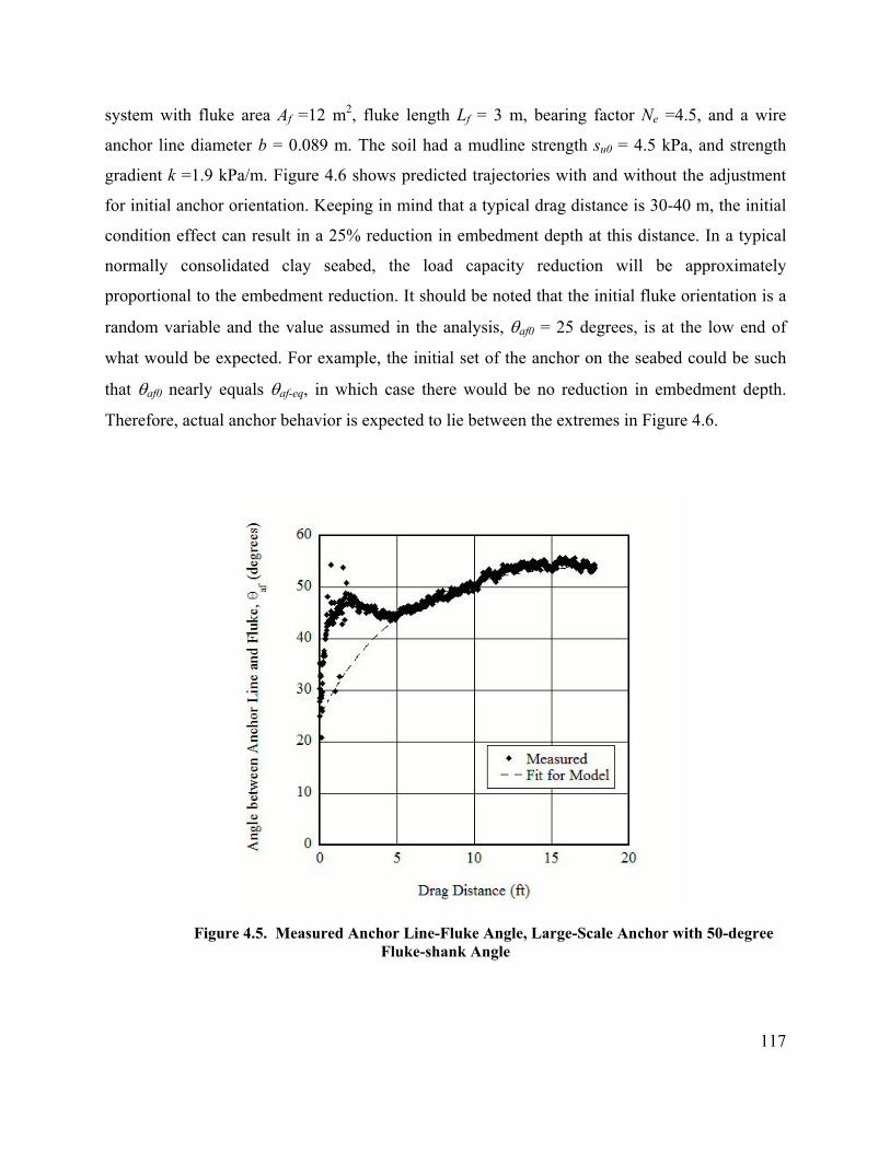
117

system with fluke area Af =12 m2, fluke length Lf = 3 m, bearing factor Ne =4.5, and a wire

anchor line diameter b = 0.089 m. The soil had a mudline strength su0 = 4.5 kPa, and strength

gradient k =1.9 kPa/m. Figure 4.6 shows predicted trajectories with and without the adjustment

for initial anchor orientation. Keeping in mind that a typical drag distance is 30-40 m, the initial

condition effect can result in a 25% reduction in embedment depth at this distance. In a typical

normally consolidated clay seabed, the load capacity reduction will be approximately

proportional to the embedment reduction. It should be noted that the initial fluke orientation is a

random variable and the value assumed in the analysis, af0 = 25 degrees, is at the low end of

what would be expected. For example, the initial set of the anchor on the seabed could be such

that af0 nearly equals af-eq, in which case there would be no reduction in embedment depth.

Therefore, actual anchor behavior is expected to lie between the extremes in Figure 4.6.

Figure 4.5. Measured Anchor Line-Fluke Angle, Large-Scale Anchor with 50-degree Fluke-shank Angle

118

It is noted that during the drag embedment tests three stages of behavior can be

considered to occur. In the first stage, the angle af between the anchor line and the fluke

transitions between its initial value and the equilibrium value as illustrated by Figure 4.5. In the

second stage, an equilibrium condition occurs in which the rate of rotation of the fluke f equals

the rate of increase in the line angle a . Under normal conditions of drag embedment, namely a

constant mudline angle 0 , this equilibrium condition maintains itself indefinitely. However, a

rapidly increasing mudline angle 0 can create a condition where the anchor line angle increases

at a faster rate than the fluke rotation, a > f . In this case the angle af will continue to increase

and apparent bearing factor Ne will correspondingly increase by virtue or Eq. 4.7. It is important

to point out that this third stage requires a rapidly increasing mudline angle that can be created

by a laboratory pulley system, but rarely occurs in the field. Accordingly, the elevated bearing

factors during the third stage should be regarded as an artifice of the laboratory setup and not

relied upon for design.

Figure 4.6. Trajectory Model Corrected for Effect of Initial Anchor Orientation

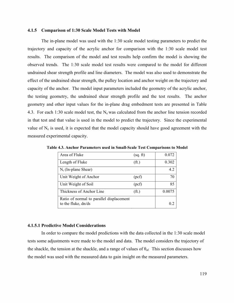
119

4.1.5 Comparison of 1:30 Scale Model Tests with Model

The in-plane model was used with the 1:30 scale model testing parameters to predict the

trajectory and capacity of the acrylic anchor for comparison with the 1:30 scale model test

results. The comparison of the model and test results help confirm the model is showing the

observed trends. The 1:30 scale model test results were compared to the model for different

undrained shear strength profile and line diameters. The model was also used to demonstrate the

effect of the undrained shear strength, the pulley location and anchor weight on the trajectory and

capacity of the anchor. The model input parameters included the geometry of the acrylic anchor,

the testing geometry, the undrained shear strength profile and the test results. The anchor

geometry and other input values for the in-plane drag embedment tests are presented in Table

4.3. For each 1:30 scale model test, the Ne was calculated from the anchor line tension recorded

in that test and that value is used in the model to predict the trajectory. Since the experimental

value of Ne is used, it is expected that the model capacity should have good agreement with the

measured experimental capacity.

Table 4.3. Anchor Parameters used in Small-Scale Test Comparisons to Model

Area of Fluke (sq. ft) 0.072

Length of Fluke (ft.) 0.302

Nt (In-plane Shear) 4.2

Unit Weight of Anchor (pcf) 70

Unit Weight of Soil (pcf) 85

Thickness of Anchor Line (ft.) 0.0075

Ratio of normal to parallel displacement to the fluke, dn/ds 0.2

4.1.5.1 Predictive Model Considerations

In order to compare the model predictions with the data collected in the 1:30 scale model

tests some adjustments were made to the model and data. The model considers the trajectory of

the shackle, the tension at the shackle, and a range of values of θaf. This section discusses how

the model was used with the measured data to gain insight on the measured parameters.

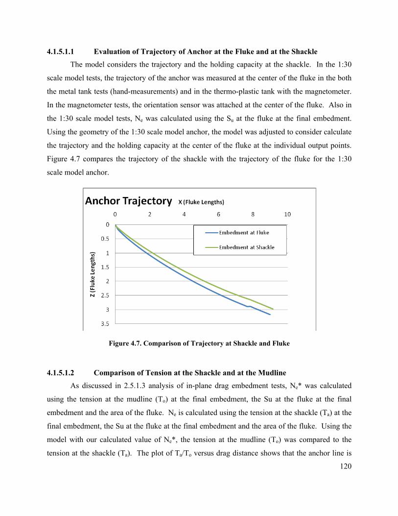
120

4.1.5.1.1 Evaluation of Trajectory of Anchor at the Fluke and at the Shackle

The model considers the trajectory and the holding capacity at the shackle. In the 1:30

scale model tests, the trajectory of the anchor was measured at the center of the fluke in the both

the metal tank tests (hand-measurements) and in the thermo-plastic tank with the magnetometer.

In the magnetometer tests, the orientation sensor was attached at the center of the fluke. Also in

the 1:30 scale model tests, Ne was calculated using the Su at the fluke at the final embedment.

Using the geometry of the 1:30 scale model anchor, the model was adjusted to consider calculate

the trajectory and the holding capacity at the center of the fluke at the individual output points.

Figure 4.7 compares the trajectory of the shackle with the trajectory of the fluke for the 1:30

scale model anchor.

Figure 4.7. Comparison of Trajectory at Shackle and Fluke

4.1.5.1.2 Comparison of Tension at the Shackle and at the Mudline

As discussed in 2.5.1.3 analysis of in-plane drag embedment tests, Ne* was calculated

using the tension at the mudline (To) at the final embedment, the Su at the fluke at the final

embedment and the area of the fluke. Ne is calculated using the tension at the shackle (Ta) at the

final embedment, the Su at the fluke at the final embedment and the area of the fluke. Using the

model with our calculated value of Ne*, the tension at the mudline (To) was compared to the

tension at the shackle (Ta). The plot of Ta/To versus drag distance shows that the anchor line is

121

becomes taut after 4 to 6 fluke lengths of drag distance (Figure 4.8). The simplified assumption

of the model that the anchor motion is governed by sliding starts to become invalid when the

anchor line becomes taut at 4 to 6 fluke lengths. It is expected that the trajectory and the holding

capacity will match the measured data within the first 4-6 fluke lengths of drag distance. Figure

4.8 also indicates that the value of To is approximately 5% greater than Ta at before the anchor

line becomes taut. Using this data, Ne*, calculated with To, can be reduced by 5% to reflect Ne

which considers that value of the tension at the shackle, Ta. When the anchor line becomes

complete taut Ta/To is approximately 1 and the model terminate the prediction. The model

terminates the output at the point when the anchor line becomes complete taut. The anchor line

is complete taut then θa=θo and Ta/To is 1.

Figure 4.8. Tension Ratio through Drag Embedment Test

4.1.5.1.3 Assessment of Anchor Line-Fluke Angle, θaf Model

The model for θaf presented in Sections 4.1.4 was adjusted to reflect the data. Equations

4.9 and 4.10 describe how the anchor transitions from θaf0 to θaf-eq. For a sample 1:30 scale

model tests in the thermo-plastic tank with the magnetometer, it was observed that θaf0

approached the equilibrium value within 1-2 fluke lengths. The χ parameter from Equation 4.9

and the λ parameter from 4.10 were adjusted to reflect the rapid change from θaf0 to θaf-eq. The

following equations were used to predict the capacity and trajectory in the 1:30 scale model tests.

122

af = af0 + 0.2 (af-eq - af0) (Revised Eq. 4.9)

af = af0 + [1- exp(-x/Lf) ] (af-eq - af0) (Revised Eq. 4.10)

where

Figure 4.9 shows the calculate values. The angle line-fluke angle, θaf –Considering a Taut

Anchor Line, was calculated by adding the pitch measurement, θf, from the magnetometer to the

anchor line angle, θa, calculated from the geometry of the testing, assuming the anchor line was

taut. The angle line-fluke angle, “θaf –Considering Reverse Catenary from Model”, was

calculated by adding the pitch measurement, θf, from the magnetometer to the anchor line angle,

θa, calculated from the model, considering the reserve catenary. The angle line-fluke angle, “θaf

–Fit to model”, shows how the Revised Eq. 4.9 and 4.10 fit the data.

Figure 4.9. Values of θaf throughout Drag Distance

4.1.5.2 Comparison of Model with Measured Data

The measured 1:30 scale model test results were compared with the model for a linearly

increasing undrained shear strength (Su) profile, for a constant Su profile, and for different anchor

line diameters. The 1:30 scale model tests were conducted in one of two test beds: a linearly

increasing undrained shear strength test bed and a constant, remolded undrained shear strength

123

test bed. Two sets of results are presented in this section are Test A from the metal tank with the

linearly increasing undrained shear strength profile and Test B test using the magnetometer in the

thermo-plastic tank with a constant, remolded undrained shear strength. Both tests were

conducted with the thick anchor line that is 0.09 in. in diameter. The input parameters are

outlined in the table below.

Table 4.4. Test bed Parameters used in Small-Scale Test Comparisons to Model

Parameter UnitsTest A - Linearly

Increasing su

Test B -Constant su with Magnetometer

Ne, equilibrium bearing capacity factor 6.21 6.22Nt (In-plane Shear) 4.2 4.5Mudline Undrained Shear Strength (psf) 0.8 25.5Shear Strength Gradient (psf/ft) 8 0.000001Initial Fluke Angle (Degrees) 35 35Horizontal Distance to Pulley (ft.) 6.25 3.33Initial Pulley Line Angle (Degrees) 5 5

4.1.5.2.1 Test A: Example Test with Linearly Increasing Su Profile

The predicted and measured anchor trajectory and holding capacity for Test A is presented in

Figure 4.10. Both the Ne* and Ne were used the model. These graphs indicate that using the Ne,

taking the tension at the shackle into account, provides a slightly better fit to the measured data.

The measured and predicted data generally match up within the first 4 fluke lengths.

124

Figure 4.10. Test A. 7/12/2010_IP_Track 2_2, in soil with linearly increasing undrained shear strength profile

125

4.1.5.2.2 Test B: Example Test with Constant Su Profile

The anchor trajectory and capacity for Test B is shown in Figure 4.11. The measured and

predicted data generally match up within the first 4 fluke lengths. The anchor capacity is very

close to the measured capacity, which is expected since the undrained shear strength is constant.

Both the Ne* and Ne were used the model. These graphs indicate that using the Ne, taking the

tension at the shackle into account, provides a slightly better fit to the measured data. The last

plot presents model and measured values of pitch (θf), the anchor line angle (θa), and the angle

between the anchor line and the fluke (θaf ). The model provides the anchor line angle (qa-model)

taking the reverse catenary into account, the angle between the anchor line and the fluke (qaf -

model) using Revised Eqn 4.9 and 4.10, and the pitch of the anchor (qf-model) from subtracting

the qa-model from qaf-model. The pitch (θf) is measured directly with the magnetometer. The θaf

is the sum of the qa-model and the measured pitch (θf). The results indicate that the model fit the

angle data better when Ne was used in the predictive model.

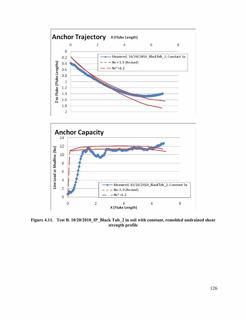
126

Figure 4.11. Test B. 10/20/2010_IP_Black Tub_2 in soil with constant, remolded undrained shear strength profile

127

Figure 4.11. Test B (cont.). 10/20/2010_IP_Black Tub_2 in soil with constant, remolded undrained shear strength profile

4.1.5.3 Comparison of Test A and B

Figure 4.12 compares the results from Test A and Test B the Ne results. The trajectory for Test

B is shorter than Test A because the pulley is located closer to the start of the test so the anchor

128

line becomes taut at a shorter drag distance, which is reflected in both the model predicted

trajectory and the testing results. Though the value of Ne was very close for these two tests, the

load capacity plot is different because of the undrained shear strength of the soil. For Test A the

undrained shear strength increases with depth, so even when Ne has reached equilibrium the load

capacity will increase as the anchor embeds itself into stiffer soils. For Test B, the soil was a

constant strength and was significant stiffer than Test A, see Table 4.4. The load capacity in Test

B is a function of Ne throughout the test, which varies slightly with θaf.

Figure 4.12. Comparison of Test A and Test B

129

4.1.5.3.1 Anchor Line Thickness

The thickness of the anchor line has an effect on the trajectory and capacity of the anchor system.

It was observed in the 1:30 scale model tests that a thinner anchor line causes the anchor to dive

deeper and the load cell readings to increase slightly. The tests were performed in the metal tank

with a linearly increasing undrained shear strength profile and the general test parameters are

listed in Table 4.4 under Test A. Figure 4.13 presents the model predicted trajectory for a thick

line (0.09 in. or Af/b2=1300) and a thin line (0.022 in. or Af/b

2=21,000). The model indicates

that the anchor’s rate of embedment is higher for the thinner anchor line, which agrees with the

measured results from the 1:30 scale model testing. Due to the testing geometry, the model

terminates the trajectory at the point where the anchor line angle (θa) is equal to the mudline

angle (θo). There will not be a significant reverse catenary developed with the thin line, so the

condition where the anchor line angle and the mudline angle are equal will be approached

quickly. Since the anchor becomes embeds quicker with a thin anchor line compared to a thick

anchor line, at the same drag distance (X) the anchor with the thin anchor line will be embedded

deeper and the undrained shear strength will be higher due to the linearly increasing Su. The two

tests had similar Ne values, 6.21 for the thick line and 6.25 for the thin line, so the increase in

load capacity is due to the higher undrained shear strength of the soil. The model fits the

measured trajectory and capacity reasonably well and indicates the trends observed in the 1:30

scale model testing.

130

Figure 4.13. Comparison of Model and Measured results with different anchor lines

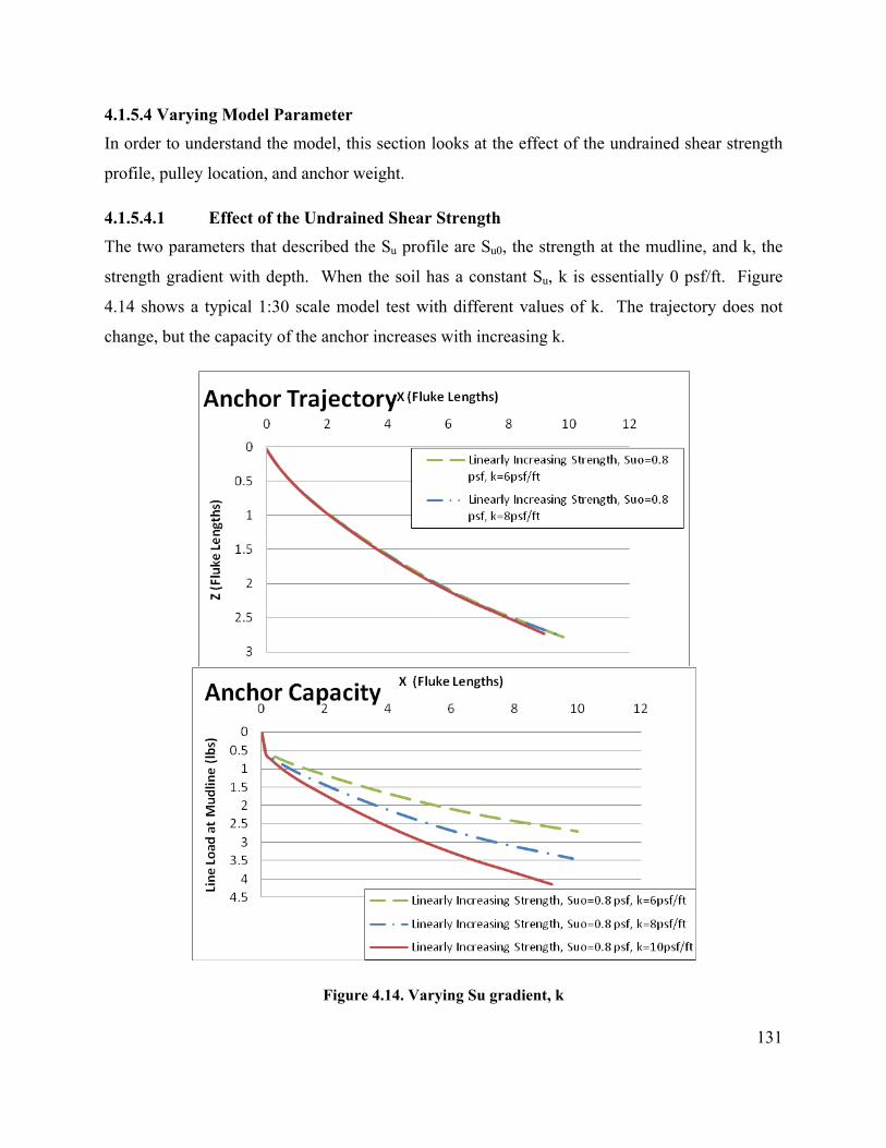
131

4.1.5.4 Varying Model Parameter

In order to understand the model, this section looks at the effect of the undrained shear strength

profile, pulley location, and anchor weight.

4.1.5.4.1 Effect of the Undrained Shear Strength

The two parameters that described the Su profile are Su0, the strength at the mudline, and k, the

strength gradient with depth. When the soil has a constant Su, k is essentially 0 psf/ft. Figure

4.14 shows a typical 1:30 scale model test with different values of k. The trajectory does not

change, but the capacity of the anchor increases with increasing k.

Figure 4.14. Varying Su gradient, k

132

Figure 4.15 shows a typical 1:30 scale model test with different values of Su0. The

general trend of the trajectory does not change, but the length of the trajectory is shorter for

higher values of Su0. When Su0 is greater, there is more effect of the reverse catenary at from the

start of the test. The model terminates the trajectory at the point when the anchor line becomes

complete taut (i.e. θa=θo). The Angle at the Mudline plot shows that θo (or qa) is increasing more

rapid when Su0 is greater. The general trend of the capacity is the same for the three tests since k

is the same, but the capacity plots are offset from each other because of the different values of

Su0.

133

Figure 4.15. Varying the Shear Strength at the mudline, Su0

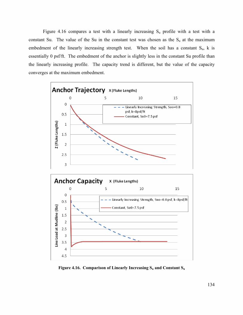
134

Figure 4.16 compares a test with a linearly increasing Su profile with a test with a

constant Su. The value of the Su in the constant test was chosen as the Su at the maximum

embedment of the linearly increasing strength test. When the soil has a constant Su, k is

essentially 0 psf/ft. The embedment of the anchor is slightly less in the constant Su profile than

the linearly increasing profile. The capacity trend is different, but the value of the capacity

converges at the maximum embedment.

Figure 4.16. Comparison of Linearly Increasing Su and Constant Su

135

4.1.5.4.2 Pulley Geometry

As discussed in Chapter 2 and 3, the in-plane drag embedment testing involves the anchor line

being pulled through a pulley. The location of the pulley affects the angle of the anchor line at

both the mudline and at the shackle, and the anchor line angle ultimately affects the embedment

of the anchor. As seen in Figure 4.17, increasing the initial tow angle (the anchor line angle

from the anchor shackle to the pulley at the start of the test) has little effect on the trajectory or

capacity of the anchor. The length of the trajectory is different, since condition where θa=θo will

be approached quicker when the tow line is steeper and the model terminates the trajectory at the

point when the anchor line becomes complete taut (i.e. θa=θo).

Figure 4.17. Varying the Initial Tow Angle of the Anchor Line

136

The location of the pulley in relation to the start of the test varied from the 1:30 scale

model test in the linearly increasing Su, 1:30 scale model test with the magnetometer in constant

Su, and the 1:10 scale model tests. Figure 4.18 compares 3 generic tests that show that pulley at

different points from the start of the test. The trajectory and capacity are essentially the same in

all the test, but the trajectory is longer for the test where the pulley is further away from the start

of the test.

Figure 4.18. Varying the Distance from the Start of the test to the Pulley

137

4.1.5.4.3 Anchor Weight

The 1:30 scale model testing was performed with an acrylic anchor, where the large scale

tests were performed with a steel anchor. Using the model we considered how the trajectory and

anchor capacity would change if the 1:30 scale model anchor was made of steel. The 1:30 scale

model anchor would weigh 0.5 pounds if it was made of steel instead of acrylic. As seen in

Figure 4.19, the results of model indicate that there would be little difference in the trajectory.

The capacity would differ slightly at the beginning of the test, but would converge later in the

drag. For the equivalent steel anchor, part of the tension in the line is used to counteract the

weight of the anchor, so the capacity is slightly less initially. For the acrylic anchor, the unit

weight of the acrylic is essentially the same as the soil, so the tension is dominated by the soil

resistance.

Figure 4.19. Comparison of the 1:30 scale model acrylic anchor and an equivalent 1:30 scale model steel anchor

138

4.2 Out-of-Plane Trajectory Behavior

Drag embedment anchors are designed assuming that the line of anchor of the anchor line force

Ta acts in the plane of symmetry of the anchor; i.e., the plane of intended loading. Under normal

conditions this assumption is reasonable. However, in the event of a partial failure of a mooring

line system; i.e., failure of one or more mooring lines in the spread, the floater can drift off

station and the anchor line force will act outside the plane of intended loading. The performance

of the remaining intact anchors under this unintended out-of-plane loading now becomes an

issue. Aubeny and Chi (2010b) present a theoretical analysis of the anticipated performance of

drag anchors under out-of-plane loading conditions, which is summarized in Section 4.2.1.

Section 4.2.2 presents an interpretation of the out-of-plane load tests conducted in this research

program that was used to evaluate the Aubeny-Chi model. Section 4.2.3 uses the model to

predict the impact of out-of-plane loading for typical field conditions.

4.2.1 Theoretical Considerations

Figure 4.20 shows a plan view of the problem under consideration. A global coordinate system,

xg- yg -zg, may be established such that zg is the vertical coordinate, xg is in the plane of intended

loading, and yg is normal to the plane of intended loading. Prior to the storm event, an in-plane

condition of loading exists, ag = 0g = 0, where the angle denotes the departure of the anchor

chain from an in-plane condition. The angles ag and 0g denote the direction of the anchor chain

measured from a horizontal plane at the pad-eye and mudline, respectively. The mudline angles

0g and 0g are arbitrarily prescribed boundary conditions for the problem. The pad-eye angles

ag and ag will be computed by a procedure to be described subsequently, but for the present we

will assume they have been defined.

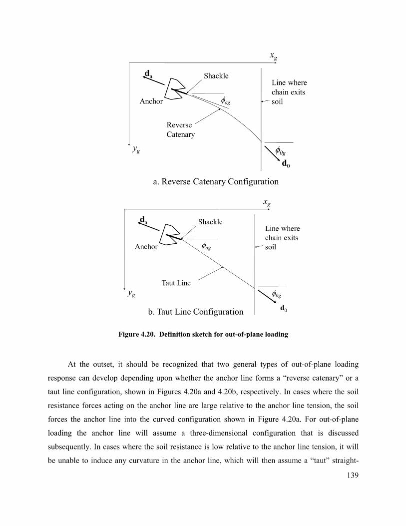
139

ShackleLine wherechain exitssoil

da

d0

xg

yg 0g

agAnchor

ReverseCatenary

a. Reverse Catenary Configuration

ShackleLine wherechain exitssoil

da

d0

xg

yg 0g

agAnchor

Taut Line

b. Taut Line Configuration

Figure 4.20. Definition sketch for out-of-plane loading

At the outset, it should be recognized that two general types of out-of-plane loading

response can develop depending upon whether the anchor line forms a “reverse catenary” or a

taut line configuration, shown in Figures 4.20a and 4.20b, respectively. In cases where the soil

resistance forces acting on the anchor line are large relative to the anchor line tension, the soil

forces the anchor line into the curved configuration shown in Figure 4.20a. For out-of-plane

loading the anchor line will assume a three-dimensional configuration that is discussed

subsequently. In cases where the soil resistance is low relative to the anchor line tension, it will

be unable to induce any curvature in the anchor line, which will then assume a “taut” straight-

140

line configuration. In cases where a taut configuration develops, the anchor response is

anticipated to simply turn into the direction of the anchor line and follow a new path in a vertical

plane oriented at 0g from the original.

Unit vectors describing the direction of the anchor chain at the shackle and mudline can then

be computed using Equations 4.11 and 4.12, respectively, as shown below:

d

ag = - [cosag cosag, cosag sinag, sinag] (Eq. 4.11)

0d

g = [cos0g cos0g, cos0g sin0g, sin0g] (Eq. 4.12)

Further, a plane containing the direction vectors d

ag and 0d

g , which shall be termed the ‘c-

plane’, can be defined in terms of the following cross product:

0 0d d / d d [ ]g ag g ag xg yg zgn n n n (Eq. 4.13)

where n is a unit vector normal to the c-plane (Figure 4.21).

Intended Loading

Out-of-PlaneVertical

MudlineDirectionVector, d0

AnchorDirectionVector, da

Oblique Plane

Normal to Oblique Planen =d0 x da

AnchorLine

Figure 4.21. Illustration of Oblique Plane Containing Anchor Chain

141

A coordinate system (xc, yc, zc) can now be defined for which the chain lies in the xc-zc

plane, subsequently termed the c-frame. It should be noted that the unit normal n to the plane of

the chain acts in the yc direction in c-frame system. The transformation is accomplished by first

rotating the xg -yg axes an angle h about the zg axis, and then rotating an angle v about the xc

axis to create an xc-yc-zc frame. The appropriate matrix relating the global g-frame to the plane

of the chain c-frame is then as follows:

cos sin 0

cos sin cos cos sin

sin sin sin cos cos

h h

gc v h v h v

v h v h v

R

(4.14)

The angles h and v are defined in term of the unit normal vector n (components nxg, nyg, nzg in the global frame) as follows:

tan h = -nxg / nyg (4.15)

sin v = nzg (4.16)

Subsequent subscripts “g” and “c” in this report refer to the global frame and the frame

oriented about the plane of the chain, respectively.

A coordinate system (xc, yc, zc in Figure 4.22) can now be defined for which the chain lies

in the xc-zc plane, subsequently termed the c-frame. It should be noted that the unit normal n to

the plane of the chain acts in the yc direction in c-frame system. The transformation is

accomplished by first rotating the xg -yg axes an angle h about the zg axis, and then rotating an

angle v about the xc axis to create an xc-yc-zc frame. The appropriate matrix relating the global

g-frame to the plane of the chain c-frame is then as follows:

142

cos sin 0

cos sin cos cos sin

sin sin sin cos cos

h h

gc v h v h v

v h v h v

R

(4.17)

The angles h and v are defined in term of the unit normal vector n (components nxg, nyg, nzg in the global frame) as follows:

tan h = -nxg / nyg (4.18)

sin v = nzg (4.19)

xglobal

yglobalzglobal

yc

xc

zc

h

v

Anchor Linein xc-zc Plane

h, vfunctions of n

Figure 4.22. Transformed Coordinate System for Out-of-Plane Loading

Subsequent subscripts “g” and “c” in this report refer to the global frame and the frame

oriented about the plane of the chain, respectively. It should be noted that the direction of the

angles follow the right-hand rule.

Having defined the frame rotation angles [Rgc], transformations of key variables from the

g-frame to the c-frame can proceed. The anchor line angle at the pad-eye ac measured in the c-

plane can be evaluated by using Equations 4.17-4.19 to determine the vector components of da

in

the c-frame, dac

= - [daxc dayc dazc], from which ac in Figure 4.23 can be calculated:

143

1tan ( )azcac

axc

d

d (4.20)

A similar transformation is possible for the anchor line angle at the mudline 0c.

fs

ac

fc

xc

zc

s in plane of chain

Anchor ChainDirection

daxc

dazc

Figure 4.23. Anchor in plane of chain

A revised form of the Neubecker and Randolph (1995) relationship between line tension

and line angles can now be derived along the same lines as the original formulation for the case

of an anchor line lying in an oblique plane:

2 20/ 2 cos / 2a ac 0c n c c u c vT E N bZ s kZ (4.21)

where Ta is anchor line tension at shackle point, En is multiplier applied to chain bar diameter,

Nc= bearing factor for wire anchor line, b = chain bar or wire diameter, su0 is the soil undrained

shear strength at mudline, k is soil strength gradient with depth, and Zc is the distance from the

anchor shackle to mudline in the zc direction.

Finally, for trajectory calculations the rate of change of ac with respect to the change in

depth can calculated in the manner described by Aubeny & Chi (2010b). When expressed in

terms of zc rather than Zc, the rate equation takes the following form:

144

2 2

2

2

ˆ ˆ2(1/ / cos )

ˆcos

n c ac 0c

c c vaac

c 0cv ac 0c

ac

E N

zTd

dz d

d

(4.22)

where ˆcz is normalized depth of shackle (= zc/b), aT is normalized tension at shackle (= Ta / sua

b2), sua is soil shear strength at the shackle, d0c/dac is the rate of change of mudline angle, c is

a strength gradient parameter (= b k cos v /su0). Therefore, the rate equation for computing the

change in ac with increasing embedment in the three-dimensional case assumes a nearly

identical form to that of an anchor contained within a vertical plane.

Having formulated the necessary transformations to describe the anchor chain in an

oblique plane, trajectory prediction can proceed according to the sequence outlined below.

1. Initial installation to an arbitrarily selected depth zi and the tension Tai corresponding to this

depth are computed using the procedure of Aubeny and Chi (2010a) developed for vertical in-

plane motion. Anchor line angles at the end of this installation stage are agi and 0gi.

2. At this point, a partial mooring failure is simulated in which the anchor line angle at the

mudline deviates from the intended plane of loading (the xglobal direction in Figure 4.22) by an

angle 0g. The anchor line angle at the pad-eye is assumed to be initially unaffected by this

change, such that ag = 0 and ag =agi. From Equations 4.11-4.17, the anchor line angles, aci

and 0ci measured in the c-plane, can be computed. Inserting these values into Equation 4.21

permits the current line tension Ta to be calculated. The calculations will show that the current

pad-eye tension is less than the original installation tension, a <ai. Therefore, as continued

loading occurs, the anchor will remain stationary and the angle ac decreases until Ta =Tai.

During this “line tautening” process, the orientation of the c-plane changes continuously as ac

changes.

3. When the line tension reaches the point at which Ta =Tai, further loading will be accompanied

by a resumption of the drag embedment process, now in the c-plane. Experience with

simulations of two-dimensional trajectories (Aubeny & Chi, 2010a) implied that a drag anchor

rapidly aligns itself with the anchor line such that the line of action of Ta acts through the

145

center of the anchor. A similar process is assumed to occur under three-dimensional loading

conditions. That is, upon resumption of the drag embedment process, the anchor is assumed to

rapidly re-align itself such that the shank lies in the c-plane.

4. Considering the orientation of the anchor in the c-plane, the orientation of the fluke will

therefore be fc = fs -ac. If the fluke advances an increment of distance s in the direction of

the fluke, then the components of displacement in the c-plane become:

xc = s cos fc (4.23)

yc = 0 (4.24)

zc = s sin fc (4.25)

The coordinates of the shackle in the global frame are accomplished through the use of the inverse of matrix [Rgc]

-1:

1

0g c

g gc

g c

x x

y R

z z

(4.26)

4.2.2 Experimental Data

The experimental measurements presented and interpreted herein are based on the laboratory

model tests described in earlier sections of this report. The focus is on verifying the assumptions

used in the development of the model presented in Section 4.2.1. It is noted that no out-of-plane

drag anchor loading data existed prior to this study, so testing the validity of the model

assumptions is extremely important. Particular issues of interest are as follows:

1. Does the anchor traverse a complex three-dimensional trajectory, or does it simply turn

toward the load and follow a trajectory in a vertical plane in the new direction of loading?

2. Does the anchor chain actually re-configure itself into an oblique plane as assumed in the

out-of-plane trajectory model?

3. Are the load capacity characteristic of the anchor (e.g., the bearing capacity factor Ne)

affected by the out-of-plane load conditions?

146

In addressing the above questions, comprehensive analyses of Haynes Laboratory Tests

96 and 98 are presented to illustrate the test interpretation procedure. This test utilized the test

setup described in Section 2 and it involved the following sequence: (1) the anchor was dragged

embedded for a prescribed distance in a direction corresponding to the “direction of intended

loading,” (2) the tow line carriage was offset a horizontal distance to achieve the desired out-of-

plane loading condition, and (3) the drag embedment process was resumed. The anchor had a

fluke-shank angle position of 50 degrees for these tests, and the tow line speed was 0.13 m/sec.

In test 96 the prescribed in-plane embedment distance was three fluke lengths, while in Test 98 it

was one fluke length.

Figures 4.24 through 4.27 show a summary of the basic measurement data for Test 96,

the nominal 15-degree out-of plane loading test. The measurements shown correspond to the

third stage of testing described above; i.e., the resumption of the drag embedment process after

the out-of-plane loading condition was imposed. Figure 4.24 shows the vertical and horizontal

tow line angles measured during the test. Measurements show the out-of-plane horizontal angle

(0g-ag in Figure 4.20) to actually be between 18-20 degrees throughout most of the test. The

initial tow line vertical angle was about 2 degrees from horizontal. Due to the shortening of the

tow line as the test progressed, this angle increased gradually to about 5 degrees in the latter

stages of the test. Figures 4.28 through 4.31 show similar data (tow line angles, trajectories) for

Test 98, which had a nominal out-of-plane load angle of 30 degrees.

Subsequent data interpretation required computation of the direction of anchor motion,

which required computation of slopes of the measured anchor trajectories in Figures 4.25-4.27

and 4.24-4.26, which required smoothing of the measurements for numerical computation of the

derivatives. To accomplish this, a weighted least squares approach was adopted to fit a local

second-order polynomial about each point where a slope computation was desired. The smooth

lines in Figures 4.25-4.27 and 4.29-4.31 show the result of the curve smoothing procedure.

Slopes of the trajectory curves were then computed through simple differentiation of the fitted

polynomials.

147

Figure 4.24. Horizontal and Vertical Tow Line Angles during 15-Degree Out-of-Plane Loading, Haynes Test 96

Figure 4.25. Measured x-z Trajectory during 15-Degree Out-of-Plane Loading, Haynes Test 96

148

Figure 4.26. Measured x-y Trajectory during 15-Degree Out-of-Plane Loading,

Haynes Test 96

Figure 4.27. Measured y-z Trajectory during 15-Degree Out-of-Plane Loading,

Haynes Test 96.

149

Figure 4.28. Horizontal and Vertical Tow Line Angles during 30-Degree Out-of-Plane Loading, Haynes Test 98

Figure 4.29. Measured x-z Trajectory during 30-Degree Out-of-Plane Loading,

Haynes Test 98

150

Figure 4.30. Measured x-y Trajectory during 30-Degree Out-of-Plane Loading,

Haynes Test 98

Figure 4.31. Measured y-z Trajectory during 30-Degree Out-of-Plane Loading,

Haynes Test 98

151

In Section 4.2.1 an analysis of the mechanics of an anchor line indicated that under

general out-of-plane loading conditions the anchor line will lie in a plane, although the plane will

not necessarily be vertical. Equations 4.11 through 4.19 were used to compute the orientation of

this oblique plane, which can be characterized in terms of a horizontal departure angle h from

the direction of initial intended loading and a vertical tilt angle v from vertical (Figure 4.22). If

the anchor line does in fact lie in an oblique plane described by the orientation angles h and v,

then anchor and anchor line movements measured in the laboratory model tests should also lie in

this plane. Since continuous measurement of motions of the shackle and tow line were made

during the tests, it is easy to determine whether these motions actually lie in the oblique plane

assumed in the model. Specifically, the chaser measurements permit a continuous time history of

the shackle velocity av

, while the tow line measurements permit a time history of anchor line

velocity at the mudline 0v

. Note that these velocities are three dimensional vectors that can be

computed in terms of the horizontal and vertical angles measured for the chaser and tow lines

throughout testing. These vectors can be used in exactly the same manner as the direction vectors

agd

and gd0

defined by Equations 4.11 and 4.12. Equations 4.13, 4.15 and 4.16 can then be used

to compute the horizontal and vertical orientation angles of the plane of motion, which should

correspond to the orientation angles h and v used in the model.

Figures 4.32 and 4.33 show the outcome of this analysis for the case of the horizontal

orientation angle of the oblique plane h. In both cases the horizontal departure angles from the

original direction of loading were in the range of 12-20 degrees. For the 15-degree out-of-plane

loading case (Test 96), this result was not unexpected. However, for the 30-degree out-of-plane

loading case (Test 98), the computed h was lower than expected. The reason for this is not clear,

but may be related to the fact that the tow line angle (Figure 4.28) was varied more in this test.

Figure 4.34 presents a definition sketch of the vertical tilt angle v of the oblique plane.

Also depicted is the fluke roll, which was measured by inclinometers in the Haynes Laboratory

tests. Figure 4.35 compares the measured vertical tilt of the plane of anchor motion to the v of

an oblique plane corresponding to an out-of-plane load angle of 15 degrees in Test 96. The

vertical tilt of the plane of motion v can be seen to vary from 35-50 degrees, and is relatively

152

constant at 35 degrees after about three fluke lengths of dragging. The tilt angle v measured for

Test 98 shown in Figure 4.36 shows that a greater out-of-plane loading angle leads to greater tilt.

In this case a 30-degree out-of-plane angle led to a tilt v of 60-70 degrees. These observations

are both qualitatively and quantitatively consistent with model predictions. Finally, it can be seen

that, while the anchor has some tendency to roll into the plane of motion, the measured roll is

much less than the measured tilt of the plane of motion. This observation may be a consequence

of the high resistance of the anchor to out-of-plane moments associated due to the large area of

the shank facing the out-of-plane direction.

153

Figure 4.32. Measured Orientation of Oblique Plane Relative to Original Plane of Loading for 15-Degree Out-of-Plane Loading, Haynes Test 96

Figure 4.33. Measured Orientation of Oblique Plane Relative to Original Plane of Loading for 30-Degree Out-of-Plane Loading, Haynes Test 98

154

Oblique Plane

AnchorRoll

Anchor Line Tilt and Anchor Roll

*Anchor Motioninto Page

Tilt, v

Figure 4.34. Definition Sketch for Anchor Roll and Anchor Line Tilt

Figure 4.35. Measurement of Anchor Roll and Oblique Plane Tilt during 15-Degree Out-of-Plane Loading, Haynes Test 96

155

Figure 4.36. Measurement of Anchor Roll and Oblique Plane Tilt during 30-Degree Out-of-Plane Loading, Haynes Test 98

As a summary response to Question 2 posed at the beginning of this section, it appears

reasonable to conclude that the anchor chain under non-taut conditions does configure itself in a

predictable oblique plane under out-of-plane loading conditions. How long the anchor chain

sustains itself in this configuration could not be fully established by the tests, due to the

limitations of the pulley system for towing the anchor. Although the anchor was dragged a fairly

large distance, the increasingly large tow line uplift angles during the latter stage of the test did

not permit a fair conclusion as to whether the anchor chain remains in an oblique plane

throughout the entire drag embedment episode or if it eventually returns into a vertical (or

perhaps slightly tilted) plane. Since the effect of tilting into an oblique plane is to reduce the

ultimate embedment depth and pullout capacity of the anchor, it is reasonable to conservatively

assume that the remains in an oblique plane configuration throughout drag embedment until

experimental evidence definitively suggests otherwise.

As defined by Eq. 4.1, the bearing factor Ne of an anchor is a critical parameter for

directly estimating anchor pullout capacity and indirectly affecting anchor trajectory during drag.

156

Load cell measurements together with the anchor fluke area and soil strength provided the data

necessary for continuous evaluation of Ne during drag embedment. As was the case for in-plane

loading, adjustment of the load cell tension measurement to account for anchor weight was

necessary using Eq. 4.6. Figures 4.37 and 4.38 show the bearing factor Ne plotted against x-

coordinate during out-of-plane drag embedment Tests 96 and 98 conducted in the Haynes

Laboratory. The value is relatively uniform throughout the test, although there was a slight

upward trend in Ne as the drag test progressed. In both tests, the sustained values of Ne = 4.4

appeared to develop. By contrast, in-plane drag embedment tests indicated a bearing factor of

about Ne = 4.

Based on the data presented above, it would appear that the response to Question 3 posed

at the outset of this section is that the bearing factor Ne under out-of-plane loading conditions

exceeds that under normal in-plane loading. While both the large-scale Haynes Laboratory tests

and the small-scale tests in the kaolin test bed (see Section 3.5.2.3) show an increase in bearing

factor, the small-scale tests show a much greater increase. For example, Tests 96 and 98

described in the preceding paragraph indicate an approximate 10% increase in bearing factor

under out-of-plane loading conditions. The small-scale tests give similar results when the

increase in undrained shear strength between in-plane tracks is considered.

157

Figure 4.37. Measured Effective Bearing Factor during 15-Degree Out-of-Plane Loading,

Haynes Test 96

Figure 4.38. Measured Effective Bearing Factor during 30-Degree Out-of-Plane Loading,

Haynes Test 98

158

4.2.3 Example Out-of-Plane Behavior

For the process described above, two variables with respect to out-of-plane loading will affect

the trajectory and capacity of the anchor following partial failure of the mooring system, the first

being the magnitude of the out-of-plane orientation angle of the chain at the mudline. The second

is the installation depth zi which failure occurs. For parametric studies, an installation penetration

ratio Rp may be defined as follows:

max

ip

zR

z (4.28)

where zmax is the ultimate embedment depth under conditions of purely in-plane loading.

As an illustrative parametric study of drag anchor trajectory predictions for out-of-plane

loading, we consider the case of drag embedment of an anchor with 12-m2 anchor in a soft clay

having zero strength at the mudline and a strength gradient k = 1.57 kPa/m. The anchor line in

this example is a wire line with diameter b = 0.089 m. Pad-eye tension was related to soil

strength at the pad-eye sua and fluke area Af by the relationship Ta = Ne sua Af, where is Ne is the

anchor bearing factor. An out-of-plane bearing factor Ne = 5 was selected for this example.

Trajectory predictions were performed for 0g = 30 degrees, and Rp was set to 0.25, 0.5, and 0.75.

The anchor line angle at the mudline was maintained in a horizontal orientation at all stages of

the simulation, 0g = 0. Simulations were performed for out-of-plane angles of 18 and 30

degrees, which roughly correspond to the Haynes Laboratory drag embedment tests discussed

earlier.

For the case of an 18-degree out-of-plane loading angle, the computed tilt v of the plane of

motion was 38 degrees. As presented earlier in Figure 4.35, the measured data for this out-of-

plane load angle indicated some scatter in v during the early stages of drag embedment, but v

stabilized at about 35 degrees after three fluke lengths of drag. For the case of a 30-degree out-

of-plane loading angle, the computed tilt v of the plane of motion was 66 degrees, which

compares well to the measured tilt angles v ranging from 60-70 degrees shown in Figure 4.36

159

for 30-degree out-of-plane loading. In summary, the model prediction of a tilted oblique plane of

motion for an anchor under out-of-plane loading is strongly supported by experimental evidence.

Table 4.5 Tilt v of Plane of Trajectory: Model Predictions versus Measurement

Out-of-Plane Angle (degrees)

Predicted v

(degrees) Measured v

(degrees) 18 38 33-50* 30 66 60-70

*After 3 fluke lengths of drag, v stabilizes to 35-40 degrees.

Figures 4.39-4.43 illustrate the practical implications of an oblique plane of motion.

Figures 4.39 and 4.40 show trajectory for 18 degrees of out-of plane loading. As expected, if out-

of-plane loading occurs at the earlier stages (lower Rp) of the drag embedment process, the effect

is most significant. In the most severe case, Rp = 0.25, an 18-degree out-of-plane load angle

results in a 25% reduction in ultimate embedment depth and load capacity. For and out-of-plane

load angle of 30 degrees, Figures 4.41-4.42 show the reduction in ultimate embedment depth to

be even more significant, about 50% for Rp = 0.25. It is noted that continued embedment occurs

following the occurrence of out-of-plane loading in all cases. However, the ultimate embedment

depth is considerably less than what would have developed had the anchor continued its

trajectory in a vertical plane. After partial failure of the mooring system, there is a modest gain in

embedment depth under sustained dragging. However, the ultimate depth is much less than that

which would develop under continued dragging within the original vertical plane of intended

loading.

The above analyses assumed no change in the anchor bearing factor during out-of-plane

loading. In fact, the experimental data indicate that the bearing factor Ne can increase by some

10-67%. Firstly, an increased Ne will directly increase the pullout capacity of the anchor.

Secondly, a greater Ne tends to increase the line tension at the pad-eye, which in turn tends to

cause the anchor to dive deeper when anchor motion resumes. Figure 4.43 shows a model

simulation of this effect for the case of 15-degree out-of-plane loading with Rp= 0.5. In this case

the anchor could conceivable dive deeper under out-of-plane loading than in-plane loading, a

scenario that was actually observed in some tests.

160

Figure 4.39. Predicted effect of 18-degree out-of-plane loading on anchor trajectory

Figure 4.40. Predicted effect of 18-degree out-of-plane loading on anchor load capacity

161

Figure 4.41. Predicted effect of 30-degree out-of-plane loading on anchor trajectory

Figure 4.42. Predicted effect of 30-degree out-of-plane loading on anchor load capacity

162

Figure 4.43. Predicted effect of increase in bearing factor on anchor trajectory during 15-degree out-of-plane loading

In summary, a complex range of possible anchor behaviors can occur under out-of-plane

loading conditions:

If a taut anchor line develops (Figure 4.20b), the anchor line is expected to simply

pivot as a straight line in a vertical plane oriented in the direction of out-of-plane

loading. Aside from the change in direction of the anchor trajectory, basic changes in

anchor behavior are not anticipated to occur.

If the anchor line forms into a reverse catenary, (Figure 4.20a), the anchor line and

anchor trajectory will lie in an oblique plane. One the one hand, the tendency for the

anchor to travel in a tilted plane will tend to reduce the ultimate embedment depth,

and therefore ultimate capacity, of the anchor. Countering this effect is an observed

increase in the anchor bearing factor, which will both cause the anchor to dive deeper

and mobilize greater pullout capacity. Therefore, the ultimate pullout capacity under

out-of-plane loading conditions could conceivably be greater than that under in-plane

loading.

163

In all cases, the anchor continues to dive under out-of-plane loading. Neither theory

nor experiment gives any indication of a reduction in the pullout capacity of the

anchor below its initial installation capacity. The worst case condition that could be

envisaged to develop is the case where the anchor bearing factor Ne does not increase

under out-of-plane loading and a reverse catenary condition forms. In this case, the

ultimate capacity of the anchor will not be as great as it would otherwise be for in-

plane loading, but it will still exceed the installation load capacity.

Based on the above findings, it appears that it is reasonable to assume no loss of the initial

installation anchor pullout capacity due to out-of-plane loading. If the anchor is loaded beyond

its initial installation load, even the most conservative assumptions of anchor behavior indicate

that continued embedment will occur with a concomitant increase in pullout capacity. Having

said this, the mechanisms of out-of-plane loading are not sufficiently well understood to justify

design recommendations for estimating the potential increase in anchor capacity under out-of-

plane loading conditions. Therefore, a reasonable, likely conservative, recommendation would be

to assume that the initial pullout capacity prevails under out-of-plane loading.

Finally, it is pointed out that the interpretations and recommendations for out-of-plane

loading behavior for DEA’s apply to out-of-plane load angles up to 30 degrees from the original

direction of intended loading.

164

5.0 Recommended Capacity Curves for Generic Anchor

Based on the revised in-plane anchor capacity prediction model discussed in Section 4, this

section presents a parametric study of anchor holding capacity for a typical normally

consolidated clay profile. The parametric study considers a strength gradient k = 1.57 kPa/m (10

psf/ft). Other factors considered in the study include:

A drag distance range from 30-100m (100-330 ft).

Wire versus chain anchor lines.

A fluke area (Af) to wire line diameter (b) ratio range Af/b2 = 1000-2000.

Fluke-shank angle settings of 50 and 36 degrees.

While anchors are typically specified in terms of their weight or mass, the primary factor

controlling their capacity is actually the fluke area Af. For the generic anchor used in this study,

the following relationship holds between fluke area and anchor mass:

2/3( ) / 31.01f aA M tonnes (Eq. 5.1)

where M is the anchor mass in Tonnes, and a is the density of the anchor material. For steel a =

7.87 Mg/m3. The factor (31.01) is a scale factor computed for the model anchor used in the

Haynes Laboratory tests. Eq. 5.1 shows a 1-tonne anchor to have a 2.5-m2 fluke and a 10-tonne

anchor to have an 11.6 m2 fluke. The anchor capacity calculations assume typical conditions of

drag embedment, specifically a horizontal mudline angle (0 = 0) throughout embedment. In all

calculations the initial orientation of the fluke with respect to the mudline was taken as 0.6 times

the fluke-shank angle for the anchor.

Figure 5.1 shows the holding capacity at the mudline for the case of 50-degree fluke-

shank setting, Af/b2 = 1500, where Af is fluke area and b is anchor line diameter. Consistent with

much of the anchor manufacturer literature, the holding capacity versus anchor weight

relationship is linear on a log-log plot. Some noteworthy points with respect to Figure 5.1

include the following:

Holding capacity increases from 50-100% as the drag distance increases from 30-100m.

165

Use of a wire line as opposed to a chain results in greater holding capacity. The holding

capacity from a chain installation can be as low as 70% of that achieved by a wire line

installation.

Empirical equations for the holding capacity curves in Figure 5.1 are tabulated in Table 1.

The holding capacity predictions in Figure 5.1 and Table 5.1 are based on a lower bound

estimate of the anchor bearing factor, Ne = 4 obtained from the large-scale anchor tests. As

discussed earlier, the small-scale tests indicated a somewhat larger bearing factor, (Ne = 5), most

likely due to the difference in fluke thickness – in relative terms the small-scale model anchor

was twice as thick as that of the large-scale anchor. Figures 5.2 and Table 5.2 show the expected

effect of the larger bearing factor, (Ne = 5) on expected holding capacity at field scale.

The relative thickness of the small-scale anchor was more representative of actual

anchors than that of the large-scale anchors, which can be construed as a justification for placing

greater weight on predictions based on the greater bearing factor, Ne = 5. However, since in-situ

marine (specifically Gulf of Mexico) clays are more sensitive than the remolded soils used in the

laboratory tests – sensitivity of about 3 for in-situ soils versus 1.5 for the kaolin test bed – it

would perhaps be more appropriate to say that the appropriate bearing factor of the generic

anchor under typical field conditions is in the likely range Ne = 4-5, and Tables 5.1 and 5.2 more

or less bound the expected holding capacities.

166

Figure 5.1. Predicted anchor capacity curves for generic anchor used in study, wire thickness ratio Af/b

2 = 1500, 50-degree fluke-shank angle with Bearing Factor Ne=4

Table 5.1. Generic Anchor Holding Capacity Relations, Af/b2 = 1500, 50-degree fluke-shank angle with Bearing Factor Ne=4

Anchor Line Type Drag Distance

(m)

Holding Capacity

(tonnes)

Wire 30 24.8W0.71

Wire 100 50.6W0.85

Chain 30 24.3W0.68

Chain 100 35.6W0.94

167

Figure 5.2. Predicted anchor capacity curves for generic anchor used in study, wire thickness ratio Af/b

2 = 1500, 50-degree fluke-shank angle with bearing factor Ne=5

Table 5.2. Generic Anchor Holding Capacity Relations, Af/b2 = 1500, 50-degree fluke-shank angle with Bearing Factor Ne=5

Anchor Line Type Drag Distance

(m)

Holding Capacity

(tonnes)

Wire 30 38.7W0.71

Wire 100 73.1W0.84

Chain 30 37.6W0.68

Chain 100 55.4W0.94

168

To evaluate the effect of the anchor line characteristics, a parametric study was conducted

for a 100-m drag distance and a wire anchor line with the line diameter varied over a range Af/b2

= 50-2000. Figure 5.3 shows the effect of wire line diameter. As is evident from the figure,

holding capacity can vary by up to a factor of 4 for the range of wire line diameters considered. It

is noted that the wire line diameter has minor influence on the anchor bearing factor. However, a

thicker wire line generates more resistance to penetration, thereby reducing the embedment depth

and, therefore, the anchor holding capacity. Table 5.3 shows empirical equations relating anchor

mass to holding capacity.

The predictions in Figures 5.1-5.3 and Tables 5.1-5.3 are for a 50-degree fluke-shank

angle. This is commonly used in soft clays, but this study also investigated the behavior of

smaller fluke-shank settings, notably a 36-degree setting. As discussed earlier, the large-scale

experimental data indicated a bearing factor Ne = 3.2 for the generic anchor at a 36-degree fluke-

shank angle setting. Figure 5.4 and Table 5.4 show the model predictions for the smaller bearing

factor. Comparison of the holding capacities for the 36-degree setting to the corresponding large-

scale anchor values in Figure 5.1 and Table 5.1 indicates that the smaller angle produces holding

capacities that are 50-67% of those corresponding to the larger setting.

A final consideration is the effect of the soil strength profile. For a normally consolidated

soil, the soil strength profile is essentially linear. In this case, the anchor embedment depth is

independent of depth, so the holding capacity simply scales with strength gradient. For example,

if the strength gradient k is 50% greater than the 1.57 kPa/m (10 psf/ft) used to develop the

relations discussed herein, holding capacity will correspondingly increase by 50%.

In summary, in addition to anchor size, anchor holding capacity depends on (1) drag

distance, (2) the use of a wire line versus a chain, (3) line or chain stock diameter, and (4) soil

strength gradient. The anchor trajectory-capacity model presented in this report provides a

predictive framework for assessing the effect of these variables as illustrated by the preceding

discussion.

169

Figure 5.3. Predicted effect of wire line diameter on anchor holding capacity for 100-m drag distance, 50-degree fluke-shank angle

Table 5.3. Generic anchor holding capacity relations for wire anchor lines with 100-m drag distance, 50-degree fluke-shank angle with Ne=4

Fluke Area to Line Diameter Ratio

Af/b2

Holding Capacity

(tonnes)

50 42.9 W0.87

500 42.9 W0.87

1000 42.9 W0.87

1500 50.6 W0.84

2000 55.6 W0.84

170

Figure 5.4. Predicted anchor capacity curves for generic anchor used in study, wire thickness ratio Af/b

2 = 1500, 36-degree fluke-shank angle

Table 5.4. Generic Anchor Holding Capacity Relations, Af/b2 = 1500, 36-degree fluke-shank angle

Anchor Line Type Drag Distance

(m)

Holding Capacity

(tonnes)

Wire 30 19.3W0.67

Wire 100 33.6W0.87

Chain 30 17.6W0.71

Chain 100 22.6W0.97

171

6. Conclusions and Recommended Future Work

Conclusions

This report presents the findings of a study on the performance of drag embedment anchors

(DEAs) in clay and loaded under undrained conditions. The following research activities were

performed: (1) small (1:30) scale model tests, (2) large (1:10) scale model tests, (3) data analysis,

(4) evaluation and calibration of a simplified predictive model, and (5) extrapolation from the

predictive model to prototype-scale field conditions. The investigations addressed anchor

behavior under in-plane and out-of-plane loading conditions. The experimental component of the

research involved test-bed soil preparation, strength characterization of test-bed soils,

development of loading systems for in-plane and out-of-plane loading, instrumentation of the

anchor and anchor line systems.

Both series of tests utilized generic anchors having fluke and shank configurations that

are reasonably representative of DEA’s used in practice. The results from the testing and how it

was used to improve the predictive model are summarized below.

1. Anchor resistance under pure loading conditions.

In pure normal bearing, the 1:30 and 1:10 scale models provided almost identical

resistances with a normal bearing factor (load normal to the fluke) of

approximately 11. This normal bearing factor is most important for a vertically

loaded anchor; a typical drag embedment anchor will never mobilize this

resistance due to the relatively flat loading angle relative to the plane of the fluke.

In pure shear, the 1:30 and 1:10 scale models (both with a 50-degree fluke-shank

angle) provide different resistance due to the different relative fluke thicknesses.

The 1:30 scale model has a larger bearing factor in pure shear than the 1:10 scale

model (4.2 versus 2.6) because the 1:10 scale model has a relatively thinner fluke:

the fluke length-to-thickness ratio (Lf/tf ) was 29 for the 1:30 scale model and 58

for the 1:10 scale model. For a typical full-scale anchor, the Lf/tf ratio ranges from

approximately 5 to 30. The 1:10 scale model was intentionally designed with a

thinner fluke so that the anchor would not sink into the soil under its own weight.

172

This shear bearing factor is very important for drag embedment anchors because

this resistance is mobilized over the majority of the drag and at the ultimate

holding capacity.

In pure pitch rotation, the 1:30 scale model has a bearing factor of 2.4. This

bearing factor is important in drag embedment at the start of the drag where the

anchor rotates until the pure shear resistance governs its behavior.

2. In-plane drag embedment tests.

The in-plane drag conditions for both the 1:30 and 1:10 scale anchor models were

reasonably comparable to typical full-scale field applications where the typical

drag distance is 10-30 fluke lengths, the typical dive distance is 3-5 fluke lengths,

and the typical holding capacity is 5-20 times the anchor’s weight in air. In the

1:30 scale tests, the drag distance was approximately 10 fluke lengths, the dive

distance averaged 2.7 fluke lengths, and the holding capacity was 6 to 9 times the

anchor weight in air (considering the anchor to be an equivalent steel anchor). In

the 1:10 scale tests with the 50-degree fluke-shank angle, the drag distance was

approximately 15 fluke lengths, the dive distance was approximately 2.5 to 3.5

fluke lengths, and the holding capacity was 4 to 4.5 times the anchor weight in air.

The model anchors achieved a constant equilibrium bearing factor, Ne = measured

load divided by divided by soil strength and fluke area, during the drag trajectory

within a relatively short drag distance of one to two fluke lengths. This factor is of

practical significance because the holding capacity can be readily estimated from

the undrained shear strength of the clay if this factor is known for a given anchor.

The model anchors also achieved a constant equilibrium angle between the anchor

line and the fluke, θaf, during the drag trajectory within a relatively short drag

distance of one to two fluke lengths. The mobilization of this constant angle over

the trajectory after the first one to two fluke lengths means that the trajectory of

the anchors during most of the drag was governed by their bearing capacity in

pure shear. This equilibrium angle between the line and the fluke, θaf, can be

calculated from force equilibrium based on the measured values for the

equilibrium bearing factor and the pure shear bearing factor. These calculated

173

values match closely to measured values for this angle, which supports the

simplifying assumption that the trajectory is governed by the bearing capacity in

pure shear.

The equilibrium bearing factor during drag for the 1:30 scale anchor model with a

50-degree fluke-shank angle was about 6 with an associated equilibrium line-

fluke angle of about 45 degrees. In comparison, the equilibrium bearing factor

during drag for the 1:10 scale anchor model with a 50-degree fluke-shank angle

was about 4 with an associated equilibrium line-fluke angle of about 55 degrees.

These results are consistent with the different geometries for the two model

anchors. The 1:30 scale anchor has a thicker fluke, a larger resistance to pure

shear, a larger resistance to drag once the equilibrium condition is reached and

therefore a flatter equilibrium angle between the line and the fluke during drag.

The 1:10 scale anchor has a thinner fluke, a smaller resistance to pure shear, a

smaller resistance to drag once the equilibrium condition is reached and therefore

a steeper equilibrium angle between the line and the fluke during drag.

The simplifying assumption that the trajectory is governed by the bearing capacity

in pure shear and the associated values for the equilibrium bearing capacity factor

and line-fluke angle were not affected by an undrained strength varying with

depth. In 1:30 scale model anchor tests with different profiles of undrained shear

strength (both constant and increasing linearly with depth), the drag resistance

was proportional to the undrained shear strength at the depth of the fluke during

drag. The profile of undrained shear strength also affected the trajectory; stronger

soil near the mudline increased the reverse catenary in the anchor line and

reduced the trajectory.

The simplifying assumption of that the trajectory is governed by the bearing

capacity in pure shear was reasonable provided that the line angle at the mudline

is relatively flat and the line did not become taut in the soil. In the 1:30 scale

model anchor tests, the behavior seemed to deviate from this assumption when the

line angle at the mudline exceeded 20 to 25 degrees to the horizontal. In the 1:10

174

scale model anchor tests, the behavior was consistent with this assumption for line

angles at the mudline up to 20 degrees.

The depth of anchor embedment decreased as the diameter of the anchor line

increased due to the interaction between the line and the soil. For the 1:30 scale

model anchor in a normally consolidated clay, the embedment was about 50

percent greater with a thin anchor line (line diameter equal to

/21,000) compared to a thicker anchor line (line diameter equal to

/1,300).

The equilibrium bearing factor decreased as the fluke-shank decreased. For the

1:10 scale model anchor, the equilibrium bearing factor was 3.2 for a 36-degreee

fluke-shank angle versus 4.0 for a 50-degree fluke-shank angle. For normally

consolidated clays, a wider fluke-shank (on the order of 50 degrees) is typically

used in practice.

Both the 1:30 and the 1:10 scale model anchor experienced some rolling during

in-plane drag embedment tests, but generally it was less than about 20 degrees

and did not seem to affect the trajectory or the line load.

3. Out-of-plane drag embedment tests. Tests with out-of-plane anchor line orientations as

high as 30 degrees and subsequent model interpretations indicated the following:

In both the 1:30 and 1:10 scale model tests with out-of-plane load angles up to 30

degrees, the equilibrium bearing factor for out-of-plane loading was equal to if

not slightly larger than that for in-plane loading because the anchor quickly turned

into the direction of the load and continues its trajectory. This result was obtained

in both the 1:30 and 1:10 scale model tests when the anchor was initially (before

out-of-plane loading) dragged in anywhere from one to three fluke lengths.

Detailed measurements of the anchor line direction and anchor trajectory in the

1:10 scale model tests (anchor line diameter equal to /256 )

indicated that the anchor line under out-of-plane loading developed a reverse

catenary in an oblique (non-vertical) plane.

175

4. Predictive model

a. The predictive model estimates anchor holding capacity considering the following

variables: anchor size, fluke-shank angle, drag distance, anchor line or chain stock

diameter, wire line versus chain systems, and soil strength profile. As illustrated

by Figures 5.1-5.3 and Tables 5.1-5.3, these variables can exert a large influence

on anchor holding capacity. Accordingly, the predictive model used in this

research has a significant advantage over the commonly used design charts, which

typically do not permit assessment of all of the relevant variables listed above.

b. The model predictions agreed well with the observed and measured results for in-

plane loading from both the 1:30 and 1:10 scale model anchor tests.

c. The predictive model was also successful in explaining measured results for out-

of-plane loading from both the 1:30 and 1:10 scale model tests. The model

predicts that the oblique catenary of the anchor line under out-of-plane loading

will slightly reduce the depth of embedment but also increase the drag resistance

of the line in the soil and that these two affects may counter-balance one another.

In spite of this generally positive assessment regarding the effects of out-of-plane

loading, it is pointed out that this research is the first attempt both experimentally

and analytically to investigate the process. In spite of the insights gained in this

research, many questions remain. At this point it is considered reasonable to

assume that there will be no reduction of initial installation holding capacity under

out-of-plane loading. Additional reserve capacity may exist, but further studies

are recommended before reliable quantitative estimates could be made.

Recommended Future Work

This research has highlighted a number of areas that merit further investigation. Particularly

pressing needs are as follows:

Effect of Anchor Geometry on Load Capacity. One outcome of this research was to

quantify the bearing factor for a generic anchor for various fluke-shank angle settings. In

addition, a widened-fluke variant of the original design was tested. The findings indicated

that anchor geometry – i.e., fluke-shank angle, fluke thickness, fluke width, shank

176

configuration – all have significant influence on the anchor bearing factor, which controls

both anchor trajectory and anchor capacity. Although some variations in anchor geometry

were considered in this study, a test matrix encompassing the full range of geometries for

anchors used in practice is still needed. Since drag anchors used in practice typically have

complex three-dimensional geometries, the most reliable and cost-effective means for

evaluating their load capacity characteristics; i.e., bearing factor. A study for evaluating

anchor load capacity as a function of anchor geometry would have two main thrusts as

outlined in this study: (1) load tests under “pure” loading (translation normal and parallel

to fluke, and rotation), and (2) drag embedment tests to evaluate the effective bearing

factor during drag embedment.

Effect of Taut Line Conditions. During a number of tests in this study, particularly the

out-of-plane tests, the anchor line transitioned from a “reverse catenary” configuration to

a “taut” state for which the anchor line exhibits essentially no curvature. The anchor

trajectory model developed and refined in this research implicitly assumes that the anchor

line is a reverse catenary; therefore, the model needs to be expanded to accommodate the

possibility of a taut anchor line condition. It is important to note that a taut anchor line

will affect both anchor trajectory and the effective bearing factor of the anchor. In

addition, while the formation of a taut line is relatively uncommon for drag embedment

anchors, it can be much more common for vertically loaded anchors (VLAs). Indeed,

conventional installation procedures for VLAs involve shortening the mooring line to

trigger the shear pin, so taut anchor line conditions may be likely to develop during this

process. Therefore, improving our understanding of anchor behavior under taut anchor

line condition will be an important step in extending the DEA trajectory-capacity model

developed in this study to VLAs. The main thrusts of this recommended research effort

would be: (1) analytical studies to formulate a theoretical framework for predicting

anchor behavior under taut line conditions, and (2) laboratory model tests of anchor

behavior under taut line conditions.

Effect of Initial Anchor Orientation. The model tests in this study shed a great deal of

light on the effect of the initial anchor orientation on DEA trajectory and, very

significantly, how a unique trajectory appears to develop that is essentially independent

177

of the initial anchor orientation. The DEA trajectory-capacity model was modified to

simulate this behavior, but two tasks remain: evaluating and modifying as necessary the

exact form of the equation used to modify the original program, and establishing a

reliable means for selecting the model parameters ( and in the current version)

required for this equation. The main thrusts of this recommended research effort would

be: (1) additional laboratory model tests where the initial anchor orientation is

systematically varied, and (2) analytical studies to support the validation and

modification of the model.

178

ReferencesAndersen K.H., Murff, J.D., Randolph, M.R. (2003). Deepwater anchor design practice -

Vertically Loaded Drag Anchors. Phase II report to API/Deepstar JIP, Volume III. Aubeny, C. P., and Chi, C. (2010a), “Mechanics of Drag Embedment Anchor in a Soft Seabed”,

Journal of Geotechnical and Geoenvironmental Engineering, ASCE. Aubeny, C.P. and Chi, C.-M. (2010b) “Trajectory prediction for DEA’s under out of plane

loading,” in review for International Symposium on Frontiers in Offshore Geotechnics, University of Western Australia, Perth.

Aubeny, C.P.; Gilbert, R.B.; Lee, C.H.; Lupulescu C.; Murff J.D.; and Yang M. (2008). Out of Plane Loading of Plate Anchors Analytical and Experimental Modeling. Offshore Technology Reach Center. November 2008.

Chen, W., and Randolph, M. (2004). Radial stress changes around caissons installed in clay by jacking and by suction. Proceedings of the 14th International Offshore and Polar Engineering Conference, Toulon, France, May 23-28, pp. 493-499.

Clukey, E.C., Phillips, R. (2002). Centrifuge model tests to verify suction caisson capacities for taut and semi-taut legged mooring systems. Proceedings of the 14th annual Deep Offshore Technology Conference for Deep Water Oil Exploration and Drilling, New Orleans, Louisiana, November 13-15.

Coffman, R.A. (2003). Horizontal capacity of suction caissons in normally consolidated clay. M.Sc. Thesis, The University of Texas at Austin.

El-Gharbawy, S.L. (1998). The pullout capacity of suction caisson foundations for tension leg platforms. Ph.D. Dissertation, The University of Texas at Austin.

El-Gharbawy, S., and Olson, R. (1999). Suction caisson foundations in the Gulf of Mexico. Proceedings of the OTRC '99 Conference, Austin, Texas, April 29-30, pp. 281-295.

El-Sherbiny, R. (2005). Performance of suction caisson anchors in normally consolidated clay. Ph.D. Dissertation, The University of Texas at Austin.

Fuglsang, L.D., and Steensen-Bach, J.O. (1991). Breakout resistance of suction piles in clay. Proceedings of the International Conference Centrifuge 91, Boulder, Colorado, pp. 153-159.

House, A.R., and Randolph, M.F. (2001). Installation and pull-out of stiffened suction caissons in cohesive sediments. Proceedings of the 11th International Offshore and Polar Engineering Conference, Stavanger, Norway, June 17-22, Vol. 2, pp. 574-580.

Kroncke, M.W. (2009) “Experimental modeling for in-plane and out-of-plane loading of scaled model drag embedment anchors,” Master's thesis, The University of Texas at Austin, Austin.

Larsen (1989). Suction anchors as an anchoring system for floating offshore constructions. Proceedings of the 21st annual Offshore Technology Conference, Houston, Texas, OTC 6029, May 1-4, pp. 535-540.

Lee, C. H. (2008). Constructing test beds of clay with a specified profile of Undrained shear strength versus depth. Ph.D. Dissertation, The University of Texas at Austin.

Neubecker, S. R., and Randolph, M. F. (1995). “Profile and frictional capacity of embedded anchor chain,” Journal of Geotechnical Engineering.

Stewart, D. P., & Randolph, M. F. (1994). T-Bar Penetration Testing in Soft Clay. Journal of Geotechnical Engineering , 2230-2235.