The Long-Run Non-Neutrality of Monetary Policy: A General Statement in a Dynamic General Equilibrium Model

Eric Kam1

Ryerson University

John Smithin2 York University

Aqeela Tabassum3 Humber College

Abstract This paper provides an explanation of the long-run neutrality of monetary policy in a dynamic general equilibrium model with micro-foundations. If the rate of time preference is endogenous there is no natural rate of interest. Therefore, if the central bank follows an interest rate rule this will affect the real rate of interest in financial markets and thereby the real economy. In principle, there is a negative relationship between the real rate of interest and the rate of inflation. This turns out to be nothing other than the historical “forced savings effect”, or the twentieth century Mundell-Tobin effect.

JEL Classifications B12, B22, B26, E13, E43, E58 Keywords Monetary non-neutrality, endogenous time preference, neo-Wicksellian models, dynamic general equilibrium models, interest rate rules 1 Eric Kam is Associate Professor of Economics at Ryerson University, Toronto, Canada M5B2K3, erickam@ryerson.ca 2 John Smithin is Professor Emeritus of Economics and Senior Scholar at York University, Toronto, Canada M3J1P3, jsmithin@yorku.ca 3 Aqeela Tabassum is Lecturer in Economics at The Business School at Humber College, Toronto, Canada M8V4B6, aqeela.tabassum@humber.ca

1

1. Introduction The idea of the long-run neutrality of changes in monetary policy is part of the DNA of the

“Classical” approach to economic theory, going back at least to Hume in 1752 (Humphrey 1998,

8-9). Of course, there have always been challenges to this position. Historically, for example, the

so-called “forced savings effect” (Hayek 1932, 1939, Humphrey 1983, Smithin 2013, 2018) was

often treated as a sort of exception that proves the rule to the general theoretical presumption of

monetary neutrality. In the mid-twentieth century there was considerable discussion of the

analogous “Mundell-Tobin effect” named after the contributions of Mundell (1963) and Tobin

(1965) which also appeared to show non-neutrality (Begg 1980, 1982, Blanchard and Fisher

1989, Smithin 1980, 2013, 2018, Turnovsky 2000, Walsh 1998). However, whether in the

nineteenth century, twentieth century, or now in the twenty-first century, these sorts of

arguments have not been well received, to say the least, by the majority of economic theorists in

the mainstream of the profession.4

One argument that has frequently been made in recent decades is that a correct

understanding of the so-called “microfoundations of macroeconomics” will enable the theorist to

confidently rule out anything like a forced savings result. Walsh (1998, 48-9), for example, has

put forward a number of arguments against some of the twentieth century demonstrations of the

Mundell-Tobin effect, the most important of which is the following:

the … behavioural relationships are ad hoc in the sense that they are not explicitly based on maximizing behaviour by the agents of the model. This limitation can lead to problems when we try to understand the effects of changes in the economic environment, such as changes in the rate of inflation. The effects will depend in part, on the way in which individual agents adjust, so we need to be able to predict how the demand function for money changes if the underlying time series behaviour of the inflation process were to change ... (d)oing so will ... highlight channels leading to quite different predictions than Tobin found ...

4 See also Kam (2000, 2005), Kam and Moshin (2006), Kam and Smithin (2012a, 2012b) and Tabassum (2012).

2

Now this sort of appeal to the microfoundations is not, in fact, a generally valid argument from

either the philosophical or methodological point of view. According to King (2012, 9), for

example, there are two main problems with what he unhesitatingly calls the microfoundations

dogma, namely, “the fallacy of composition and downward causation”. Therefore:

Since the microfoundations dogma is inconsistent with both of these principles, the dogma itself must be false. (Emphasis added) Nonetheless as suggested in the quote from Walsh, and in very many other examples in the

contemporary literature, the idea that an appeal to “the” microfoundations is decisive is now

almost universally accepted among the relevant peer group of academic economists. In the

current intellectual environment, this situation in itself provides an extremely difficult challenge

for those trying to engage in meaningful debate. Therefore, Kam (2000, 2005) took a different

approach to that of King in addressing the question of monetary non-neutrality. That project was

to show that non-neutrality still applies even in a framework which arguably had impeccable

microfoundations by the standards of orthodox neoclassical economics. The purpose of the

exercise was essentially to communicate with those colleagues who may be very well-versed in

mathematical techniques, but not necessarily in questions of ontology and epistemology.

Kam’s work was based on a modification of the well-known Sidrauski model (Sidrauski

1967) which at that time had been a staple of graduate-level textbooks for many years

(Blanchard and Fisher 1989, Turnovsky 2000, Chiang and Wainwright 2005), and still is to this

day.5 However, the canonical model in twenty-first century theoretical macroeconomics is now

5 The intellectual roots of this general approach go even further back, to the works of the Cambridge mathematician and philosopher Frank Ramsey in the 1920s (Ramsey 1927, 1928). Rather obviously, Ramsey must have had his mathematical rather than his philosophical hat firmly on his head at the time when he made these contributions. Tellingly Keynes, who was the editor of the journal in which these papers were published (and also a mathematician and philosopher and colleague and friend of Ramsey) made no use whatsoever of Ramsey’s approach in either the Treatise on Money (Keynes 1930) or the General Theory (Keynes 1936).

3

one version or another of either the dynamic general equilibrium (DGE) model or the dynamic

stochastic general equilibrium (DSGE) model (DeVroey 2016, King 2012, 1, Scarth 2014,

Woodford 2010, 1-4).6 At this stage of the game it therefore also seems important (again for the

purposes of communication) to make a more general statement about the issues in the context of

a theoretical DGE model.

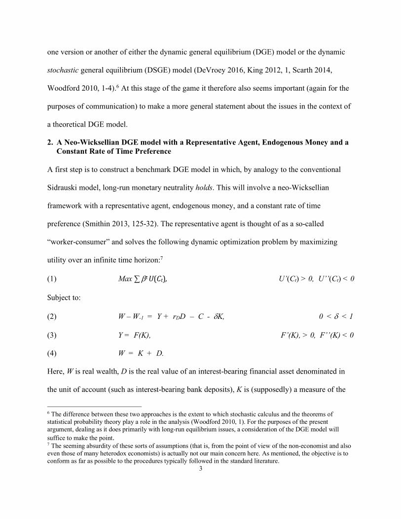
2. A Neo-Wicksellian DGE model with a Representative Agent, Endogenous Money and a Constant Rate of Time Preference

A first step is to construct a benchmark DGE model in which, by analogy to the conventional

Sidrauski model, long-run monetary neutrality holds. This will involve a neo-Wicksellian

framework with a representative agent, endogenous money, and a constant rate of time

preference (Smithin 2013, 125-32). The representative agent is thought of as a so-called

“worker-consumer” and solves the following dynamic optimization problem by maximizing

utility over an infinite time horizon:7

(1) Max ∑btU(Ct), U’(Ct) > 0, U’’(Ct) < 0

Subject to:

(2) W – W-1 = Y + rDD – C - dK, 0 < d < 1

(3) Y = F(K), F’(K), > 0, F’’(K) < 0

(4) W = K + D.

Here, W is real wealth, D is the real value of an interest-bearing financial asset denominated in

the unit of account (such as interest-bearing bank deposits), K is (supposedly) a measure of the

6 The difference between these two approaches is the extent to which stochastic calculus and the theorems of statistical probability theory play a role in the analysis (Woodford 2010, 1). For the purposes of the present argument, dealing as it does primarily with long-run equilibrium issues, a consideration of the DGE model will suffice to make the point. 7 The seeming absurdity of these sorts of assumptions (that is, from the point of view of the non-economist and also even those of many heterodox economists) is actually not our main concern here. As mentioned, the objective is to conform as far as possible to the procedures typically followed in the standard literature.

4

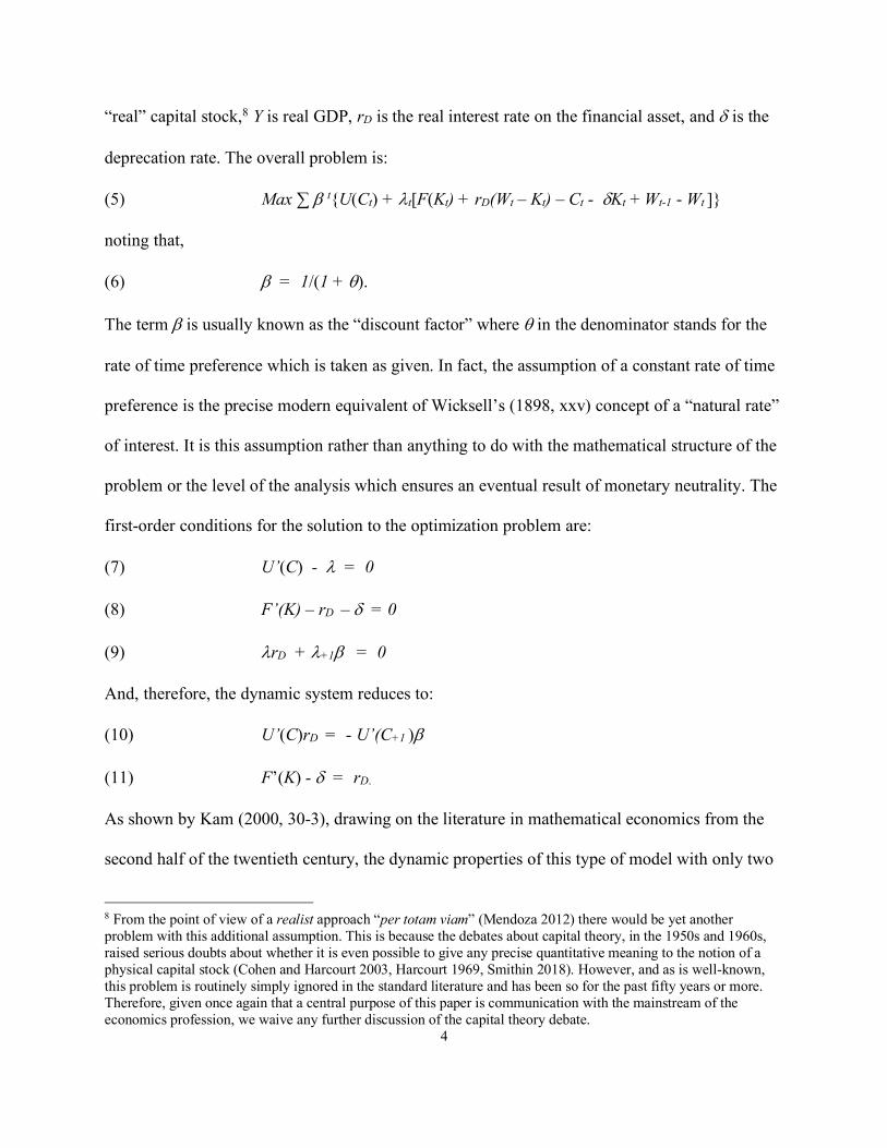
“real” capital stock,8 Y is real GDP, rD is the real interest rate on the financial asset, and d is the

deprecation rate. The overall problem is:

(5) Max ∑ b t{U(Ct) + lt[F(Kt) + rD(Wt – Kt) – Ct - dKt + Wt-1 - Wt ]}

noting that,

(6) b = 1/(1 + q).

The term b is usually known as the “discount factor” where q in the denominator stands for the

rate of time preference which is taken as given. In fact, the assumption of a constant rate of time

preference is the precise modern equivalent of Wicksell’s (1898, xxv) concept of a “natural rate”

of interest. It is this assumption rather than anything to do with the mathematical structure of the

problem or the level of the analysis which ensures an eventual result of monetary neutrality. The

first-order conditions for the solution to the optimization problem are:

(7) U’(C) - l = 0

(8) F’(K) – rD – d = 0

(9) lrD + l+1b = 0

And, therefore, the dynamic system reduces to:

(10) U’(C)rD = - U’(C+1 )b

(11) F’(K) - d = rD.

As shown by Kam (2000, 30-3), drawing on the literature in mathematical economics from the

second half of the twentieth century, the dynamic properties of this type of model with only two

8 From the point of view of a realist approach “per totam viam” (Mendoza 2012) there would be yet another problem with this additional assumption. This is because the debates about capital theory, in the 1950s and 1960s, raised serious doubts about whether it is even possible to give any precise quantitative meaning to the notion of a physical capital stock (Cohen and Harcourt 2003, Harcourt 1969, Smithin 2018). However, and as is well-known, this problem is routinely simply ignored in the standard literature and has been so for the past fifty years or more. Therefore, given once again that a central purpose of this paper is communication with the mainstream of the economics profession, we waive any further discussion of the capital theory debate.

5

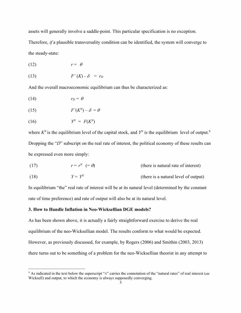
assets will generally involve a saddle-point. This particular specification is no exception.

Therefore, if a plausible transversality condition can be identified, the system will converge to

the steady-state:

(12) r = q

(13) F’ (K) - d = rD

And the overall macroeconomic equilibrium can thus be characterized as:

(14) rD = q

(15) F’(KN) – d = q

(16) YN = F(KN)

where KN is the equilibrium level of the capital stock, and YN is the equilibrium level of output.9

Dropping the “D” subscript on the real rate of interest, the political economy of these results can

be expressed even more simply:

(17) r = rN (= q) (there is natural rate of interest)

(18) Y = YN (there is a natural level of output)

In equilibrium “the” real rate of interest will be at its natural level (determined by the constant

rate of time preference) and rate of output will also be at its natural level.

3. How to Handle Inflation in Neo-Wicksellian DGE models?

As has been shown above, it is actually a fairly straightforward exercise to derive the real

equilibrium of the neo-Wicksellian model. The results conform to what would be expected.

However, as previously discussed, for example, by Rogers (2006) and Smithin (2003, 2013)

there turns out to be something of a problem for the neo-Wicksellian theorist in any attempt to

9 As indicated in the text below the superscript “N” carries the connotation of the “natural rates” of real interest (au Wicksell) and output, to which the economy is always supposedly converging.

6

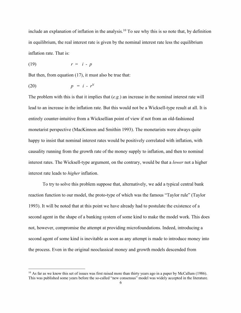
include an explanation of inflation in the analysis.10 To see why this is so note that, by definition

in equilibrium, the real interest rate is given by the nominal interest rate less the equilibrium

inflation rate. That is:

(19) r = i - p

But then, from equation (17), it must also be true that:

(20) p = i - rN

The problem with this is that it implies that (e.g.) an increase in the nominal interest rate will

lead to an increase in the inflation rate. But this would not be a Wicksell-type result at all. It is

entirely counter-intuitive from a Wicksellian point of view if not from an old-fashioned

monetarist perspective (MacKinnon and Smithin 1993). The monetarists were always quite

happy to insist that nominal interest rates would be positively correlated with inflation, with

causality running from the growth rate of the money supply to inflation, and then to nominal

interest rates. The Wicksell-type argument, on the contrary, would be that a lower not a higher

interest rate leads to higher inflation.

To try to solve this problem suppose that, alternatively, we add a typical central bank

reaction function to our model, the proto-type of which was the famous “Taylor rule” (Taylor

1993). It will be noted that at this point we have already had to postulate the existence of a

second agent in the shape of a banking system of some kind to make the model work. This does

not, however, compromise the attempt at providing microfoundations. Indeed, introducing a

second agent of some kind is inevitable as soon as any attempt is made to introduce money into

the process. Even in the original neoclassical money and growth models descended from

10 As far as we know this set of issues was first raised more than thirty years ago in a paper by McCallum (1986). This was published some years before the so-called “new consensus” model was widely accepted in the literature.

7

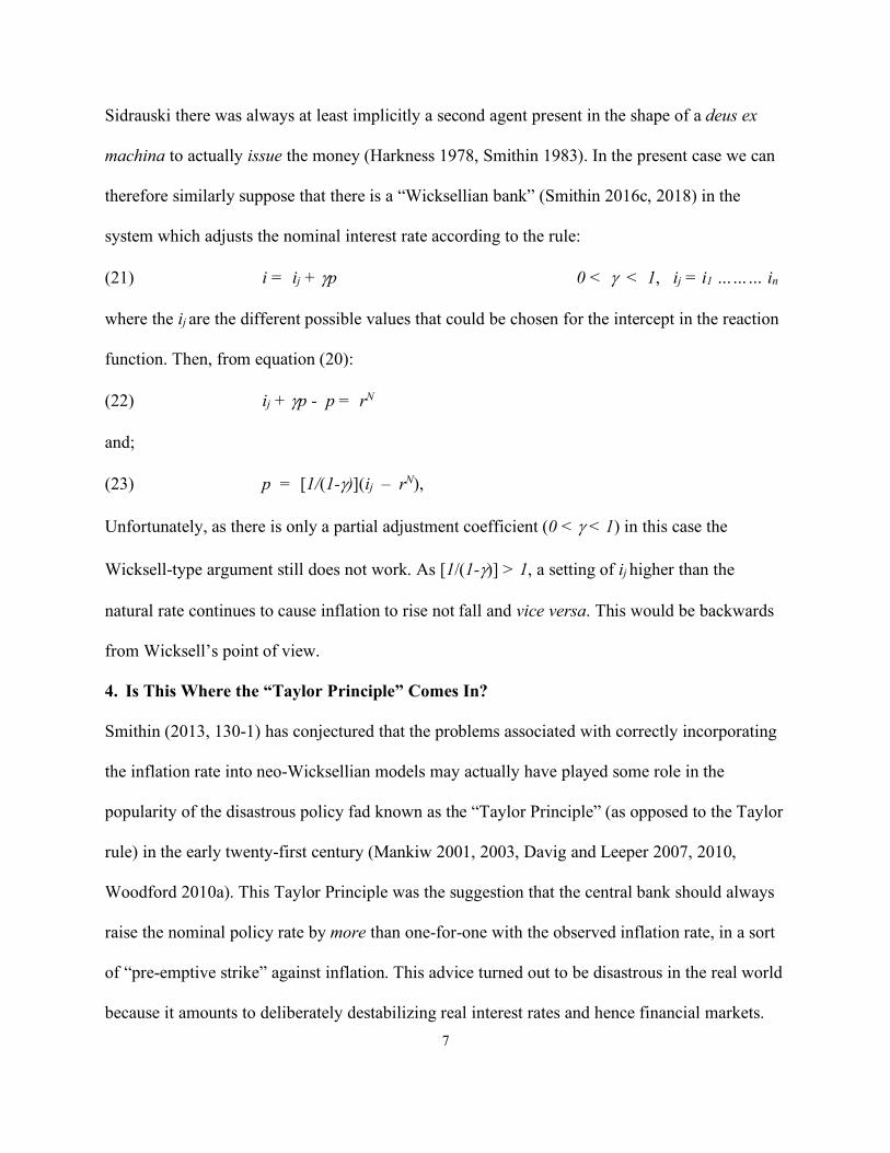
Sidrauski there was always at least implicitly a second agent present in the shape of a deus ex

machina to actually issue the money (Harkness 1978, Smithin 1983). In the present case we can

therefore similarly suppose that there is a “Wicksellian bank” (Smithin 2016c, 2018) in the

system which adjusts the nominal interest rate according to the rule:

(21) i = ij + gp 0 < g < 1, ij = i1 ……… in

where the ij are the different possible values that could be chosen for the intercept in the reaction

function. Then, from equation (20):

(22) ij + gp - p = rN

and;

(23) p = [1/(1-g)](ij – rN),

Unfortunately, as there is only a partial adjustment coefficient (0 < g < 1) in this case the

Wicksell-type argument still does not work. As [1/(1-g)] > 1, a setting of ij higher than the

natural rate continues to cause inflation to rise not fall and vice versa. This would be backwards

from Wicksell’s point of view.

4. Is This Where the “Taylor Principle” Comes In?

Smithin (2013, 130-1) has conjectured that the problems associated with correctly incorporating

the inflation rate into neo-Wicksellian models may actually have played some role in the

popularity of the disastrous policy fad known as the “Taylor Principle” (as opposed to the Taylor

rule) in the early twenty-first century (Mankiw 2001, 2003, Davig and Leeper 2007, 2010,

Woodford 2010a). This Taylor Principle was the suggestion that the central bank should always

raise the nominal policy rate by more than one-for-one with the observed inflation rate, in a sort

of “pre-emptive strike” against inflation. This advice turned out to be disastrous in the real world

because it amounts to deliberately destabilizing real interest rates and hence financial markets.

8

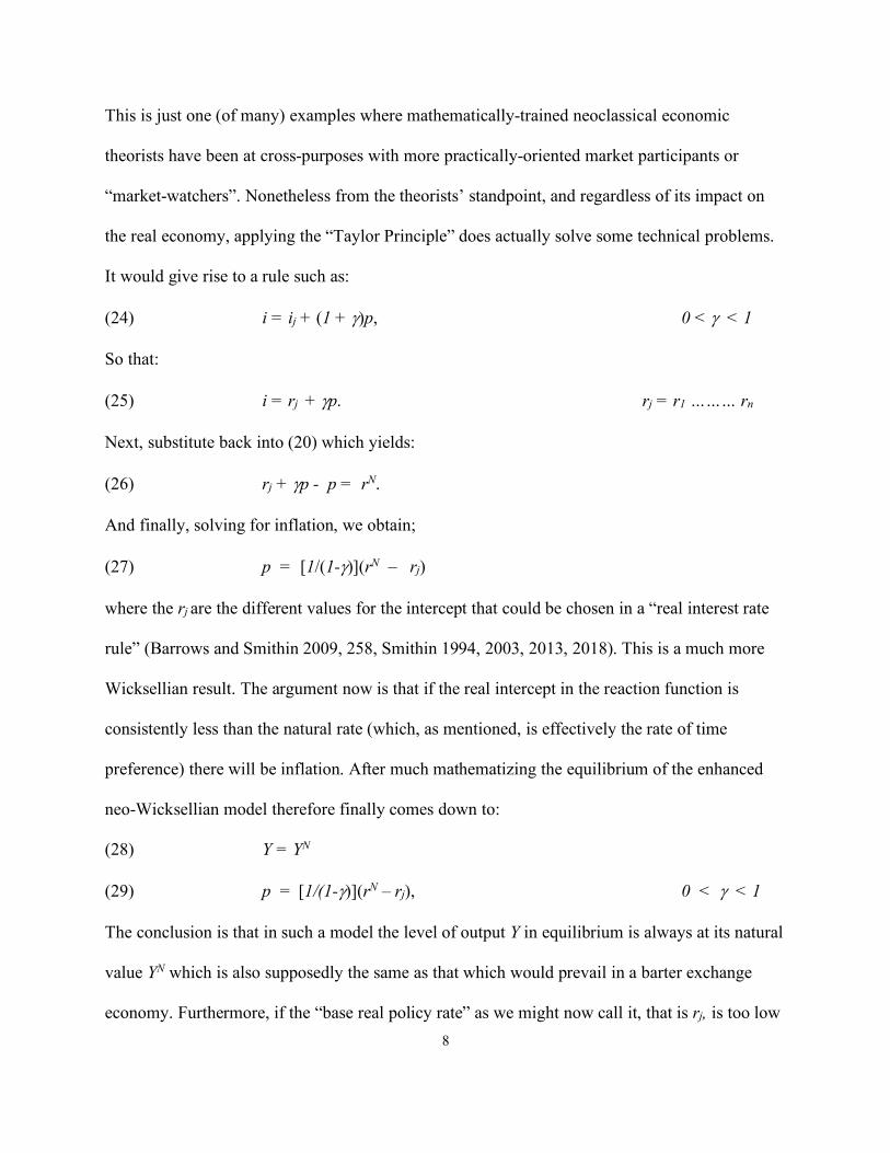
This is just one (of many) examples where mathematically-trained neoclassical economic

theorists have been at cross-purposes with more practically-oriented market participants or

“market-watchers”. Nonetheless from the theorists’ standpoint, and regardless of its impact on

the real economy, applying the “Taylor Principle” does actually solve some technical problems.

It would give rise to a rule such as:

(24) i = ij + (1 + g)p, 0 < g < 1

So that:

(25) i = rj + gp. rj = r1 ……… rn

Next, substitute back into (20) which yields:

(26) rj + gp - p = rN.

And finally, solving for inflation, we obtain;

(27) p = [1/(1-g)](rN – rj)

where the rj are the different values for the intercept that could be chosen in a “real interest rate

rule” (Barrows and Smithin 2009, 258, Smithin 1994, 2003, 2013, 2018). This is a much more

Wicksellian result. The argument now is that if the real intercept in the reaction function is

consistently less than the natural rate (which, as mentioned, is effectively the rate of time

preference) there will be inflation. After much mathematizing the equilibrium of the enhanced

neo-Wicksellian model therefore finally comes down to:

(28) Y = YN

(29) p = [1/(1-g)](rN – rj), 0 < g < 1

The conclusion is that in such a model the level of output Y in equilibrium is always at its natural

value YN which is also supposedly the same as that which would prevail in a barter exchange

economy. Furthermore, if the “base real policy rate” as we might now call it, that is rj, is too low

9

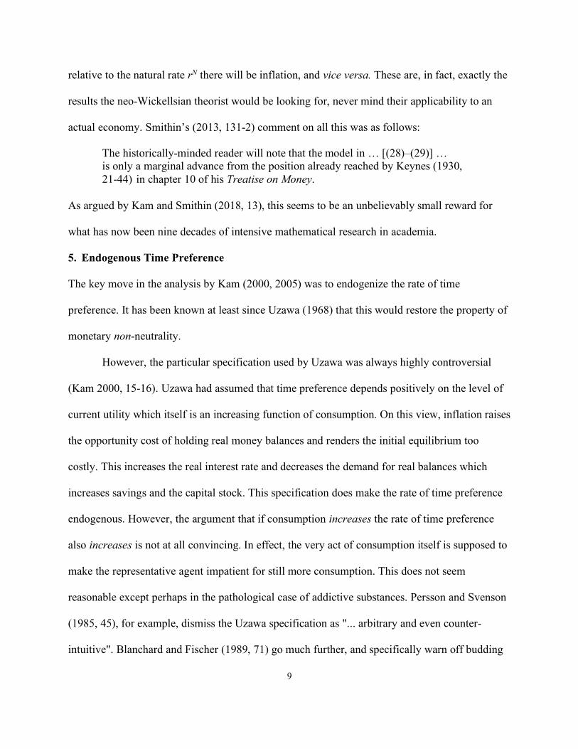
relative to the natural rate rN there will be inflation, and vice versa. These are, in fact, exactly the

results the neo-Wickellsian theorist would be looking for, never mind their applicability to an

actual economy. Smithin’s (2013, 131-2) comment on all this was as follows:

The historically-minded reader will note that the model in … [(28)–(29)] … is only a marginal advance from the position already reached by Keynes (1930, 21-44) in chapter 10 of his Treatise on Money.

As argued by Kam and Smithin (2018, 13), this seems to be an unbelievably small reward for

what has now been nine decades of intensive mathematical research in academia.

5. Endogenous Time Preference

The key move in the analysis by Kam (2000, 2005) was to endogenize the rate of time

preference. It has been known at least since Uzawa (1968) that this would restore the property of

monetary non-neutrality.

However, the particular specification used by Uzawa was always highly controversial

(Kam 2000, 15-16). Uzawa had assumed that time preference depends positively on the level of

current utility which itself is an increasing function of consumption. On this view, inflation raises

the opportunity cost of holding real money balances and renders the initial equilibrium too

costly. This increases the real interest rate and decreases the demand for real balances which

increases savings and the capital stock. This specification does make the rate of time preference

endogenous. However, the argument that if consumption increases the rate of time preference

also increases is not at all convincing. In effect, the very act of consumption itself is supposed to

make the representative agent impatient for still more consumption. This does not seem

reasonable except perhaps in the pathological case of addictive substances. Persson and Svenson

(1985, 45), for example, dismiss the Uzawa specification as "... arbitrary and even counter-

intuitive". Blanchard and Fischer (1989, 71) go much further, and specifically warn off budding

10

economic theorists by stating that:

[although the] ... specification avoids the pathological results of the constant discount rate ... the Uzawa function, with its assumption that the rate of time preference increases in instantaneous utility is not ... attractive as a

description of preferences and is not recommended for general use.

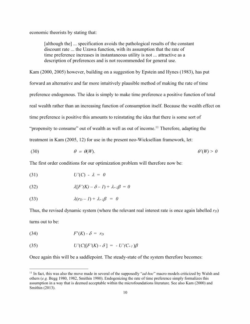
Kam (2000, 2005) however, building on a suggestion by Epstein and Hynes (1983), has put

forward an alternative and far more intuitively plausible method of making the rate of time

preference endogenous. The idea is simply to make time preference a positive function of total

real wealth rather than an increasing function of consumption itself. Because the wealth effect on

time preference is positive this amounts to reinstating the idea that there is some sort of

“propensity to consume” out of wealth as well as out of income.11 Therefore, adapting the

treatment in Kam (2005, 12) for use in the present neo-Wicksellian framework, let:

(30) q = q(W). q’(W) > 0

The first order conditions for our optimization problem will therefore now be:

(31) U’(C) - l = 0

(32) l[F’(K) – d – 1) + l+1b = 0

(33) l(rD – 1) + l+1b = 0

Thus, the revised dynamic system (where the relevant real interest rate is once again labelled rD)

turns out to be:

(34) F’(K) - d = rD

(35) U’(C)[F’(K) - d ] = - U’(C+1 )b

Once again this will be a saddlepoint. The steady-state of the system therefore becomes:

11 In fact, this was also the move made in several of the supposedly “ad-hoc” macro models criticized by Walsh and others (e.g. Begg 1980, 1982, Smithin 1980). Endogenizing the rate of time preference simply formalizes this assumption in a way that is deemed acceptable within the microfoundations literature. See also Kam (2000) and Smithin (2013).

11

(36) F’ (K) - d = rD

(37) F’(K) - d = q(W).

There is no longer any natural rate of interest in the equilibrium of this model. All of the rate of

time preference, the net marginal product of capital, and the real rate of interest on money must

conform to the standard set by the deliberate monetary policy of the Wicksellian bank (Smithin

1994, 2003, 2013, 2018). Comparing these results to those of Kam (2000, 2005), endogenizing

the rate of time preference is thus proven to break the orthodox result of long-run monetary

neutrality, regardless of whether the monetary policy instrument is the rate of growth of the

money supply itself or an interest rate.

6. A Simple Theory of Banking and the Relationship between Commercial Banks and the Central Bank

One possible interpretation of the nature of the financial asset in the optimization problem above

is as an interest-bearing deposit in (specifically) a commercial bank. In this case, logically

speaking, there would therefore have to be at least one more agent in the system in addition to

the worker-consumer and the single Wicksellian bank already posited. It now becomes necessary

to distinguish between two separate components of the banking system, namely, the commercial

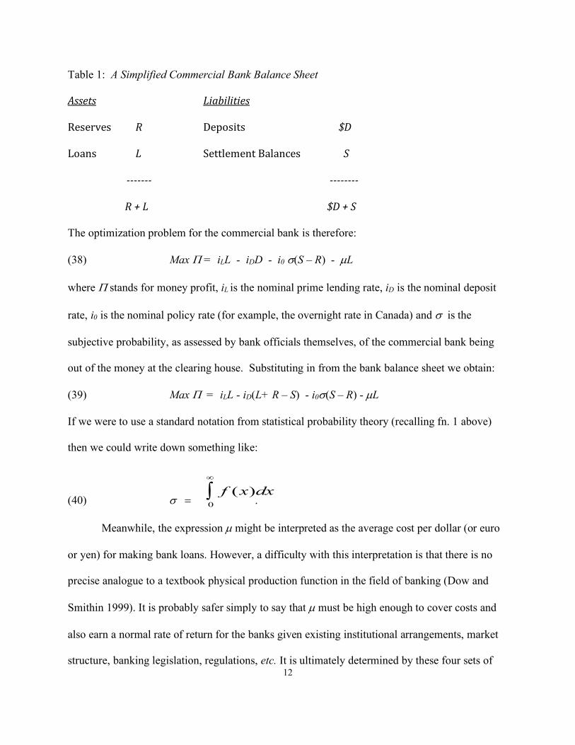
bank and the central bank. Following Kam and Smithin (2012a) therefore, let the simplified

balance sheet of the commercial bank be as follows. Here, $D stands for nominal deposits in the

commercial bank, S for any outstanding negative settlement balances of the commercial bank at

the central bank, R for nominal bank reserves, and L for the nominal dollar amount of

commercial bank loans outstanding:

12

Table 1: A Simplified Commercial Bank Balance Sheet

Assets Liabilities

Reserves R Deposits $D

Loans L SettlementBalances S

------- --------

R+L $D+S

The optimization problem for the commercial bank is therefore:

(38) Max P = iLL - iDD - i0 s(S – R) - µL

where P stands for money profit, iL is the nominal prime lending rate, iD is the nominal deposit

rate, i0 is the nominal policy rate (for example, the overnight rate in Canada) and s is the

subjective probability, as assessed by bank officials themselves, of the commercial bank being

out of the money at the clearing house. Substituting in from the bank balance sheet we obtain:

(39) Max P = iLL - iD(L+ R – S) - i0s(S – R) - µL

If we were to use a standard notation from statistical probability theory (recalling fn. 1 above)

then we could write down something like:

(40) s = .

Meanwhile, the expression µ might be interpreted as the average cost per dollar (or euro

or yen) for making bank loans. However, a difficulty with this interpretation is that there is no

precise analogue to a textbook physical production function in the field of banking (Dow and

Smithin 1999). It is probably safer simply to say that µ must be high enough to cover costs and

also earn a normal rate of return for the banks given existing institutional arrangements, market

structure, banking legislation, regulations, etc. It is ultimately determined by these four sets of

f x dx( )0

¥

ò

13

conditions. Next, substituting in from the balance sheet, the optimization problem becomes:

(41) Max: P = iLL - iD(L + R – S) - iOs(S – R) - µL

where the choice variables are the volume of loans granted and the quantity of precautionary

reserves banks choose to hold. The first order conditions are obtained by differentiating with

respect to L and R and setting the results equal to zero:

(42) iL - iD = µ

(43) iD = siO.

The mark-up between commercial bank lending rates and deposit rates is therefore equal to µ,

and the deposit rate in the commercial bank iD, is a mark-down from the central bank's setting of

the policy rate, i0. The degree of the mark-down thus depends on the subjective assessment of the

“risk” (as this is called in neoclassical economics - a true Keynesian would prefer to call it

uncertainty) if the representative commercial bank does not "[keep] in step" (Keynes 1930, 23)

with its rivals. In the past, a similar sort of result has sometimes been called the "two-for-one"

rule (Rogers and Rymes 2000, 259). However, to get a value of exactly s = 0.5 would depend

on making the twin assumptions of ergodicity and a normal distribution which are unlikely both

to hold in practice. Empirically, the value of the s term seems to be much higher than 0.5 (say

around 0.8) but still less than unity (see Collis 2018).

Combining equations (42) and (43) we can see that there is a linear relationship between

the policy rate and the commercial bank lending rate thus providing an account of how changes

in the central bank policy rate are transmitted to interest rates in general. That is:

(44) iL = µ + si0

Next, subtract the observed inflation rate, p, from both sides of equation (44):

14

(45) iL - p = µ + sr0 - (1-s)p,

Here the term r0 is the inflation-adjusted real policy rate of interest, that is, the nominal policy

rate adjusted for the currently observed inflation rate, or r0 = i0 - p. This result gives some further

insight into the several discussions over the years by Smithin (1994, 2003, 2007, 2009, 2013,

2016a, 2016b, 2018) about a "real interest rate rule" for monetary policy. As a practical matter

such a rule would have to involve a target for the inflation-adjusted policy rate (as defined

above) simply because the true expected inflation rate is not known. The question now,

therefore, is whether the similar inflation-adjusted real commercial bank lending rate in equation

(45) can also be taken as a “proxy” (Taylor 1993) for the real lending rate itself. If so, and in the

absence of any other indicator on which the borrowers can base their estimates, equation (45)

may be re-written as:

(46) r = µ + sr0 - (1-s)p

Where term r now stands for the real interest rate actually involved in economic decision-making

such as, for example, the interest rate in an investment function or in an “IS curve” in a macro

model. Equation (46) thus shows how central bank activities do indeed have an influence over

the real rate of interest in the market-place, and thereby on the real economy in general. Notice

particularly, that there is negative theoretical relationship between inflation and the real rate of

interest in this situation. This is nothing other than the forced saving (or Mundell-Tobin) effect,

as already discussed.

7. A Real Interest Rate Rule for Monetary Policy?

From equations (42) and (43), we can see that it also must be the case that:

(47) rD = sr0 - (1-s)p

This formulation raises the possibility that at least in principle the central bank could pursue a

15

feedback rule intended to fix the real rate of return on the financial asset (the bank deposits)

actually held by the representative worker-consumer in our model. To set rD = r’, for example,

the central bank must follow the rule:

(48) r0 = (1/s )r’ + [(1-s)/s)]p

In and of itself this rule is quite complicated and in actual practice any rule followed by the

central bank is presumably going to have to be much more straightforward, such as the various

suggestions put forward in Smithin (2009, 2013, 2016a, 2016b).12 In the real world central

bankers will not be able to cover every contingency and therefore their main objective should be

not to add to instability (unlike in the case of their adherence to the Taylor Principle).

Nonetheless, if we are prepared to allow that, in principle, the central bank could follow such a

rule (that is, given an exact knowledge of the parameters) this would greatly simplify the

theoretical model and thereby help us to better understand some of that model’s basic features

(see Kam and Smithin 2012b and Smithin 2013, 2018). This, therefore, will be the underlying

assumption in the theoretical discussion to follow.

8. Is there a “User Cost” of Producing Capital Goods rather than Consumption Goods?

There is still one loose-end to be tied up. As we have now abandoned the Taylor Principle per se,

the system no longer determines the inflation rate. We are therefore back to the dilemma

originally faced by theorists of the new consensus in their “models without money” (Rogers

2006, Smithin 2009, Woodford 1998) at the end of the twentieth century and the beginning of the

twenty-first, discussed above. This failing, however can be remedied merely by introducing

some frictions into the problem of our representative worker-consumer. Evidently one of the

main choices that the agent faces is whether to allocate current output to investment goods (that

12 Smithin (2016a, 2016b, 2018) has also shown that a real rate rule will ensure inflation stability.

16

is, to increase the capital stock) or to consumption. We can therefore reasonably suppose that

there is some sort of lump-sum user cost that must be incurred when making these changes.

Let V be the nominal user cost and P the price level. According to the usual logic of

profit maximization or cost minimization there must therefore be a further marginal condition for

the representative worker-consumer as follows:

(49) V/P = F’(K)

Next suppose that nominal user costs, in what we have supposed to be necessarily a money-using

system, evolve according to:

(50) V = V0P-1 V0 > 1

Substituting (48) into (47) we obtain:

(51) V0(P-1)/P = F’(K)

which implies:

(52) V0/F’(K) = (1 + p)

This therefore suggests a positive relationship between the level of real output and inflation due

to the frictions associated with switching production from consumer goods to capital goods in a

monetary economy. The underlying reason for this is that the user costs have to be paid in terms

of money (i.e., from bank deposits).

9. Formal Results

Drawing now on each of equations (11), (37) and (52) reported above, the solution system for the

complete macroeconomic model is as follows:

(53) F’ (K) - d = r’

(54) q(K + D) = r’

(55) V0/F’(K) = (1 + p)

17

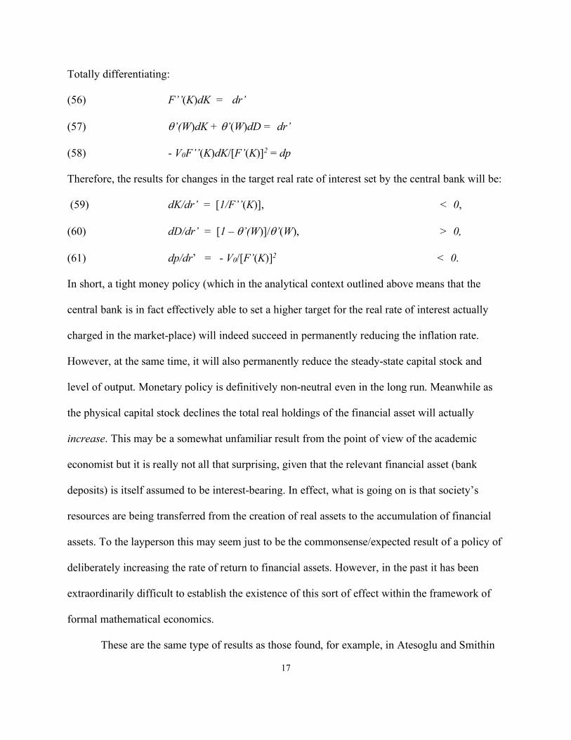
Totally differentiating:

(56) F’’(K)dK = dr’

(57) q’(W)dK + q’(W)dD = dr’

(58) - V0F’’(K)dK/[F’(K)]2 = dp

Therefore, the results for changes in the target real rate of interest set by the central bank will be:

(59) dK/dr’ = [1/F’’(K)], < 0,

(60) dD/dr’ = [1 – q’(W)]/q’(W), > 0,

(61) dp/dr’ = - V0/[F’(K)]2 < 0.

In short, a tight money policy (which in the analytical context outlined above means that the

central bank is in fact effectively able to set a higher target for the real rate of interest actually

charged in the market-place) will indeed succeed in permanently reducing the inflation rate.

However, at the same time, it will also permanently reduce the steady-state capital stock and

level of output. Monetary policy is definitively non-neutral even in the long run. Meanwhile as

the physical capital stock declines the total real holdings of the financial asset will actually

increase. This may be a somewhat unfamiliar result from the point of view of the academic

economist but it is really not all that surprising, given that the relevant financial asset (bank

deposits) is itself assumed to be interest-bearing. In effect, what is going on is that society’s

resources are being transferred from the creation of real assets to the accumulation of financial

assets. To the layperson this may seem just to be the commonsense/expected result of a policy of

deliberately increasing the rate of return to financial assets. However, in the past it has been

extraordinarily difficult to establish the existence of this sort of effect within the framework of

formal mathematical economics.

These are the same type of results as those found, for example, in Atesoglu and Smithin

18

(2006, 2007), Collis (2018) Kam (2000, 2005), Mackinnon and Smithin (1993), Smithin (2003,

2009, 2013, 2018) and Tabassum (2012) and they are therefore robust across a wide variety of

different model specifications. From the point of view of the mainstream economist, the chief

thing that should be interesting about them is that, in this treatment, the so-called

“microfoundations” have been provided in detail. It is therefore no longer possible to simply

dismiss the non-neutrality findings on a priori methodological grounds.

10. Conclusion

This paper has provided an explanation of the long-run non-neutrality of monetary policy in the

context of a neo-Wicksellian DGE model with microfoundations. If the rate of time preference in

endogenous there is no “natural rate” of interest. Therefore, if the central bank pursues a real

interest rate rule this will influence the real levels of both the lending and deposit rates in the

commercial banks and will affect the real economy via this route. There is a negative relationship

between the inflation-adjusted real lending rate of the commercial banks and the rate of inflation

itself. This is nothing other than the old “forced saving” effect or the twentieth century Mundell-

Tobin effect.

19

References Atesoglu, H. Sonmez and John Smithin. 2006. Inflation targeting in a simple macroeconomic model. Journal of Post Keynesian Economics 28: 673-688. Atesoglu, H. Sonmez and John Smithin. 2007. Un modelo macroeconomico simple. Economia Informa 346: 105-19. Barrows, David and John Smithin 2009. Fundamentals of Economics for Business (2nd edition), Toronto and Singapore: Captus Press and World Scientific Publishing. Begg, David K.H. 1980. Rational expectations and the non-neutrality of monetary policy. Review of Economic Studies 47: 293-303. Begg, David K.H. 1982. The Rational Expectations Revolution in Macroeconomics: Theories and Evidence, Baltimore: John Hopkins University Press. Blanchard, Olivier and Stanley Fischer. 1989. Lectures on Macroeconomics. Cambridge, MA: MIT Press. Chiang, Alpha C. and Colin Wainwright. 2005. Fundamental Methods of Mathematical Economics (fourth edition). New York: McGraw-Hill. Cohen, Avi and G.C. Harcourt. 2003. Whatever happened to the Cambridge capital controversies? Journal of Economic Perspectives 17: 199-214. Collis, Reed. 2018. Three Essays on Monetary Macroeconomics: An Empirical Examination of the Soundness of the Alternative Monetary Model and Monetary Policy in Canada. PhD thesis in Economics, York University, Toronto. Davig, Troy and Eric M. Leeper. 2007. Generalizing the Taylor principle. American Economic Review 97: 603-35. Davig, Troy and Eric M. Leeper. 2010. Generalizing the Taylor principle: reply. American Economic Review 100: 618-24. DeVroey, Michel. 2016. A History of Macroeconomics: From Keynes to Lucas and Beyond. Cambridge: Cambridge University Press. Dow, Sheila C. and John Smithin. 1999. The structure of financial markets and the “first principles” of monetary economics. Scottish Journal of Political Economy 46: 72-90. Epstein, Larry G. and Allan J. Hynes. 1983. The rate of time preference and dynamic economic analysis. Journal of Political Economy 91: 611-35. Harcourt G.C. 1969. Some Cambridge controversies in the theory of capital. Journal of Economic Literature 7: 369-405.

20

Harkness, Jon. 1978. The neutrality of money in neoclassical growth models. Canadian Journal of Economics 11: 701-13. Hayek, Friedrich A. 1932. A note on the development of the doctrine of “forced saving”. Quarterly Journal of Economics 47: 123-33. Hayek, Friedrich A. 1939. Introduction. To An Inquiry into the Nature and Effects of the Paper Credit of Great Britain by Henry Thornton. (As reprinted by Augustus M. Kelley, New York: 11-63, 1991). Humphrey, Thomas. 1983. Can the central bank peg real interest rates: a survey of classical and neoclassical opinion Federal Reserve Bank of Richmond Economic Review. (As reprinted in Money Banking and Inflation, 35-44, Aldershot: Edward Elgar, 1993). Humphrey, Thomas. 1998. Mercantalists and classicals: insights from doctrinal history. Federal Reserve Bank of Richmond: Annual Report, 2-27. Kam, Eric. 2000. Three Essay on Endogenous Time Preference, Monetary Non-Superneutrality and the Mundell-Tobin Effect. PhD thesis in Economics, York University, Toronto. Kam, Eric. 2005. A note on time preference and the Tobin effect. Economics Letters 89: 137-42. Kam, Eric and Mohammed Mohsin. 2006. Monetary policy and endogenous time preference. Journal of Economic Studies 33: 52-69. Kam, Eric and John Smithin. 2012a. A simple theory of banking and the relationship between commercial banks and the central bank. Journal of Post Keynesian Economics 34: 545-49. Kam, Eric and John Smithin. 2012b: Capitalism in one country: a re-examination of mercantilist systems from the financial point of view. In L-P. Rochon and S.Y. Olawoye (eds.), Monetary Policy and Central Banking: New Directions in Post-Keynesian Theory, Cheltenham: Edward Elgar, 37-52. Keynes, John Maynard. 1930. A Treatise on Money (2 vols). (As reprinted in Collected Writings Vols. V & V1, (ed.) Donald Moggridge, London: Macmillan, 1971) Keynes, John Maynard. 1936. The General Theory of Employment Interest and Money. (As reprinted by Harcourt Brace: London, 1964.) King, John. 2012. The Microfoundations Delusion. Cheltenham: Edward Elgar. McCallum, Bennett T. 1986. Some issues concerning interest rate pegging, price level determinacy and the real bills doctrine. Journal of Monetary Economics 17: 139-68. MacKinnon, Keith T. and John Smithin. 1993. An interest rate peg, inflation and output. Journal of Macroeconomics 15: 769-85.

21

Mankiw, Gregory N. 2001. US monetary policy during the 1990s. NBER Working Paper 8471, September. Mankiw, Gregory N. 2003. Program report: monetary economics. NBER Reporter, 1-5, Spring. Mendoza Espana, Alberto d’A. 2012. Three Essays on Money, Credit and Philosophy: A Realist Approach per totam viam to Monetary Science. Ph.D thesis in Economics, York University. Mundell, Robert A. 1963. Inflation and real interest. Journal of Political Economy 71: 280-83. Ramsey Frank P. 1927. A contribution to the theory of taxation. Economic Journal 37: 45-61. Ramsey Frank P. 1928. A mathematical theory of saving. Economic Journal 38: 543-59. Rogers Colin. 2006. Doing without money: a critical assessment of Woodford’s analysis. Cambridge Journal of Economics 30: 293-306. Rymes, T.K. 1998. Keynes on anchorless banking. Journal of the History of Economic Thought 20: 71-82. Rymes, T.K. and Colin Rogers. 2000. The disappearance of Keynes's nascent theory of banking between the Treatise and the General Theory. In What is Money? (ed.) John Smithin, 255-69, London: Routledge. Scarth, William M. 2014. Macroeconomics: The Development of Modern Methods for Policy Analysis. Cheltenham: Edward Elgar. Sidrauski, Miguel. 1967. Rational choice and patterns of growth in a monetary economy. American Economic Review: 57: 534-44. Smithin, John. 1980. On the sources of the super-neutrality of money in the steady-state. Working Paper 80-14, Department of Economics, McMaster University, October. Smithin, John. 1983. A note on the welfare cost of perfectly anticipated inflation. Bulletin of Economic Research 35: 65-69. Smithin, John. 1994. Controversies in Monetary Economics, Ideas, Issues, and Policy. Aldershot: Edward Elgar. Smithin, John. 2003. Controversies in Monetary Economics: Revised Edition. Cheltenham: Edward Elgar. Smithin, John. 2007. A real interest rule for monetary policy? Journal of Post Keynesian Economics 30: 101-18.

22

Smithin, John. 2009. Money, Enterprise and Income Distribution: Towards a Macroeconomic Theory of Capitalism. London: Routledge, 2009. Smithin, John. 2013. Essays in the Fundamental Theory of Monetary Economics and Macroeconomics. Singapore: World Scientific Publishing. Smithin, John. 2016a. Endogenous money, fiscal policy, interest rates and the exchange rate regime: a comment on Palley, Tymoigne, and Wray. Review of Political Economy 28: 64-78. Smithin, John. 2016b. Endogenous money, fiscal policy, interest rates and the exchange rate regime: correction. Review of Political Economy 28: 609-11. Smithin, John. 2016c. Some puzzles about money, finance, and the monetary circuit. Cambridge Journal of Economics 40: 1259-74. Smithin, John. 2018. Re-thinking the Theory of Money, Credit and Macroeconomics: A New Approach for the Twenty-First Century. Lanham MD: Lexington Books. Smithin, John and Eric Kam. 2018. Hicks on Hayek, Keynes, and Wicksell. In Economic Growth and Macroeconomic Stabilization Policies in Post-Keynesian Economics: Essays in Honour of Marc Lavoie and Mario Seccareccia: Book Two. H. Bougrine and L-P. Rochon (eds.), Cheltenham: Edward Elgar. Tabassum, Aqeela. 2012. Three Essays on the Impact of Financial Evolution on Monetary Policy Ph.D thesis in Economics, York University, Toronto. Taylor, John. 1993. Discretion versus policy rules in practice. Carnegie-Rochester Conference Series on Public Policy 39: 195-214. Tobin, James. 1965. Money and economic growth. Econometrica 33: 671-4. Turnovsky, Stephen. 2000. Methods of Macroeconomic Dynamics (second edition). Cambridge, MA: MIT Press. Uzawa, Hirofumi. 1968. Time preference, the consumption function, and optimal asset holdings. In Value, Capital, and Growth: Essays in Honour of Sir John Hicks, (ed.) J.N. Wolfe, 485-504, Edinburgh: Edinburgh University Press. Walsh, Carl E. 1998. Monetary Theory and Policy. Cambridge MA: Cambridge University Press. Wicksell. Knut. 1898. Interest and Prices: A Study of the Causes Regulating the Value of Money. (As reprinted by Augustus M. Kelley: New York, 1965) Woodford, Michael. 1998. Doing without money: controlling inflation in a post-monetary world. Review of Economic Dynamics 1: 173-219.

23

Woodford, Michael. 2003. Interest and Prices: Foundations of a Theory of Monetary Policy. Princeton NJ: Princeton University Press. Woodford, Michael. 2010a. The simple analytics of the government expenditure multiplier. NBER Working Paper 15714, January. Woodford, Michael. 2010b. Robustly optimal monetary policy with near-rational expectations American Economic Review 100: 274-303.