1

Long run effects of short-term non-neutrality of mo ney

Stefan Collignon

A paper prepared for Institut für Makroökonomie und Konjunkturforschung (IMK) in der Hans-

Böckler-Stiftung Abstract. The long run neutrality hypothesis of money (LRN) states that monetary policy can only affect real economic variables in the short run, but not in the long run. However, this hypothesis depends crucially on the role assigned to the labour market. This paper looks at long run effects resulting from capital accumulation that shift the labour demand curve and the Phillips curve. It is shown that an investment function based on Tobin’s q can explain long-term shifts in the capital stock, which respond to short-term interest rates set by monetary policy. Empirical evidence supports the theoretical model. JEL classification: E24, E31, E4,E5

www.stefancollignon.eu

2

Long run effects of short-term non-neutrality of mo ney

Table of Content

I. The Theory of Non-Neutrality of Money ..................................................................... 5

Labour market equilibrium and the natural rate of unemployment ................................ 5 The demand for Labour .............................................................................................. 6 Labour supply ............................................................................................................. 7

A reformulated Phillips curve ......................................................................................... 9 Wage setting .............................................................................................................. 10 Price setting .............................................................................................................. 11 The modified Phillips curve ...................................................................................... 13

Capital market equilibrium and the mark-up ................................................................ 14 Determining the price level ....................................................................................... 15 The mark-up and interest rates ................................................................................. 19 Determining the capital stock ................................................................................... 20

II. Empirical Evidence for Non-Neutrality of Money.................................................. 22 The data ......................................................................................................................... 22

Interest rates ............................................................................................................. 23 Investment ................................................................................................................. 25 Tobin’s q ................................................................................................................... 27

The long-term effects of short-term variation in Tobin’s q .......................................... 30 The VAR model ......................................................................................................... 30 Results ....................................................................................................................... 31

Estimating the modified Phillips curve ......................................................................... 35 The ARMA model ...................................................................................................... 35 The results ................................................................................................................. 36

Conclusion ....................................................................................................................... 38 Bibliography ................................................................................................................. 39

Appendix .......................................................................................................................... 43 Data ............................................................................................................................... 43 VAR .............................................................................................................................. 43

3

Long run effects of short-term non-neutrality of mo ney Stefan Collignon1

"Neutrality of money" is a basic tenet of economics. A model is said to exhibit money

neutrality if a change in the level of nominal money does not affect real variables.

Superneutrality applies the same concept to changes in the rate of growth of nominal

money and asks whether such changes on capital accumulation, output and welfare

(Orphanides and Solows, 1990). For reasons, which will become clear later on, I will not

always distinguish between neutrality and superneutrality in this paper. The concept of

neutrality of money is closely related to Friedman’s and Phelps’ natural rate of

unemployment model. The long-run neutrality of money (LRN) hypothesis states that

monetary policy can only affect real economic variables in the short run, but not in the

long run. An expansionary monetary policy can help the economy to come out of a

recession and return faster to its long-run equilibrium (the natural level), but it cannot

sustain higher output forever. The validity of the hypothesis depends critically on the

assumption that individuals are free of "money illusion", i.e. are concerned only by “real”

variables and not by nominal claims - implying that prices are flexible, markets

competitive and agents have full information2. The economy is then modelled as a system

of homogeneous demand functions, where excess demand in the real sector depends on

relative prices of goods and demand in the monetary sector depends on relative prices

and the initial quantity of monetary assets, so that an excess supply of money causes the

price level to rise (Patinkin, 1989). Therefore, in equilibrium money is neutral by

definition.

This neutrality is reflected in the long run correlation between prices and money

(Friedman and Schwartz, 1982), although this relationship does not prove causality.

McCandless and Weber (1995), covering a 30-year period and 110 countries, have found

that the correlation between inflation and growth of money supply is almost one, while

1 London School of Economics and Harvard University. I would like to thank Pedro Gomes and Antoine Nebout for research assisatance. 2 But of course, the opposite is not true : Non-neutrality of money does not imply money illusion.

4

there is no correlation between these variables and the growth rate of real output. They

find a positive correlation for a sub-sample of OECD-countries, where the correlation

between real growth and money growth (but not inflation) is positive. However, in recent

years the focus has shifted away from monetary aggregates, as monetary policy is

targeting inflation and uses interest rates to preserve price stability (Woodford, 2003).

Barro (1995) observed a negative correlation between inflation and growth in a cross-

country sample, while Bullard and Keating (1995) found evidence for a permanent shift

in inflation producing positive growth effects in low-inflation countries and zero or

negative effects for high inflation countries. Fisher and Seater (1993), Logeay and Tober

(2003), Kunzin and Tober (2004) also have produced evidence that money may not be

neutral in the long-term.

The long-run empirical regularities of monetary economies are important for gauging

how well the steady-state properties of a theoretical model match the data (Walsh, 1998).

Short-run dynamic relationship between money inflation and output reflect the way in

which private agents and monetary authorities respond to economic disturbances. Most

economists recognize that monetary disturbances can have important effects on real

variables in the short run. As Lucas (1996: 604) summarized the debate: "this tension

between two incompatible ideas – that changes in money are neutral unit changes and

that they induce movements in employment and production in the same direction – has

been at the centre of monetary theory at least since Hume".

In this paper, I will argue that the neutrality and superneutrality of money depends on the

variable under consideration. First of all, I will focus on changes in interest rates, which

are the principal monetary policy instrument rather them looking at monetary aggregates.

The question is how short-term shocks translate into long-term phenomena. While

monetary shocks may have transitory effects on some variables, these effects may

accumulate over time. This is most obvious with respect to investment. For example if

prices or wages are sticky, then it is well known that monetary policy may be able to

induce changes in output or investment in the short-run. Over time, as prices adjust, the

system reverts to the equilibrium steady state of output and investment, although the level

5

of output and employment may be higher. Thus, money appears superneutral with respect

to the rate of growth and investment in the long-term. But the temporary increase in

investment would have caused a permanent increase in the stock of capital and therefore

also in the equilibrium level of output and employment. Money is non-neutral with

respect to these variables. Monetary policy is therefore, also not neutral with respect to

the natural level of unemployment.

The rest of the paper is structured as follows. I will first outline a theoretical model where

monetary policy shifts the Philips curve in the long run, so that there is non-neutrality of

money with respect to employment. In the second part I will provide evidence for long-

term effects of monetary policy on the capital stock in a sample of European countries.

I. The Theory of Non-Neutrality of Money

To establish the theoretical claim that short-term non-neutrality of money has long run

effects, we will start with the basic assumptions of the natural rate of unemployment

model, then reformulate the Phillips curve as being dependent on the profit share rather

than the real wage and finally introduce the capital market in the model.

Labour market equilibrium and the natural rate of unemployment

If money is neutral in the long run, aggregate supply must be determined by non-

monetary factors. Neoclassical economics derives the vertical long-term supply curve

from equilibrium in the labour market at the so-called natural rate of unemployment,

which reflects the market position where real wages equalise demand and supply for

labour. Firms employ labour up to the level where real wages are covered by the marginal

product of labour. Output is then determined by the technological parameters of the

production function and the price level by the quantity of money. Because wage earners

are only interested in what money can buy, they bargain over real wages and there are no

real effects caused by money other than creating short-term or temporary disturbances.

Goods’ prices and interest rates, i.e. prices in the other markets of the Walrasian system,

6

cannot influence output or unemployment systematically3. However, this result depends

on the fact that the labour market equilibrium is independent from other markets,

especially the capital market. In neoclassical model, the monetary sector adjusts to real

variables in the long run. However, it is also possible that monetary policy decisions and

financial markets are the exogenous variable, taken by investors maximising the return of

their asset portfolio; in this case, financial markets may have systematic effects on real

variables.

The demand for Labour

To prove our claim, we start with a simple neoclassical model of the labour market.

Firms produce output with a homogenous production function using labour (L) and

capital (K) at given technology (τ):

(1) ),( KLFY τ= with 0,0,0,0,0 ><<>> LKKKLLKL FFFFF

We define average labour productivity, i.e. the output per employee as:

(1a) ( )kfLY τ==Λ ( ) 0>′ kf , ( ) 0<′′ kf

with the capital intensity LKk = . ( )kf ′ is the marginal product of capital per unit of

labour. τ reflects Hicks-neutral technology at constant capital intensity. Firms employ

labour up to the level where short-term profits are maximised. Profits are defined as

revenue minus the wage bill, so that short-term profits are maximised by equalling the

marginal product of labour to real wages at a given capital stock K :

(2) max WLLKFPWLPY −=−=Π ),(τ

with P the price level, W as the nominal wage, and K the given capital stock.

As is well known, the solution yields that profits are maximised when the real wage

equals the marginal product of capital:

(2a) ( )P

WKLFL =,

3 A similar result is obtained by letting wage bargainers and price setters make nominal claims; the equilibrium is then obtained by the non-accelerating inflation rate of unemployment (NAIRU)

7

For future reference we also define the wage share as a function of real wages and

productivity:

(2b) Λ

== 1P

W

PY

WLwσ or in logs: 4 λ−−= pwsw (wage share)

And the profit share as the part of aggregate income that goes to capital.

(2c) kwPY

WLPY

PYσσ =−=−=Π

1 (profit share)

The profit share is the complement of the wage share and is maximised at a given level of

capital stock when labour receives the marginal product as real wage, so that in a

neoclassical setting, the profit share is determined by the ratio of marginal to average

productivity of labour.5

The demand for labour by profit maximising firms is a function of the real wage and the

capital stock employed.

(2d)

Φ= KP

WLD ,

By totally differentiating we get:

(2e) KdFFPWdFdL LLLKLLD )/()/()/1( −=

In the short run, the capital stock remains constant. The demand curve for labour is

downward sloping, because 0<LLF , but in the long-run an increase in the capital stock

can shift labour demand up.

Labour supply

Because workers face a trade-off between leisure and consumption, labour supply is

assumed to be an increasing function in the real wage and depending on a vector of shift

parameters X:

4 Small letters denote logs, unless otherwise specified.

5 Assuming (2b), the optimal neoclassical wage share is ,*)(

)*,(_

kf

KLFL

τ where */*

_

LKk = and L* the

level of employment when the real wage equals the marginal product. If the real wage is exogenous, short term profit maximizers will adjust labour productivity by changing capital intensity.

8

(2f)

= XP

WLs ,ϕ

The slope of the labour supply curve 0/ >pwϕ is a measure for structural wage and price

flexibility. The literature has produced a long list of factors X, which might shift the

labour supply curve exogenously. Typically it includes population growth, the reservation

wage, the replacement ratio, factors affecting the job match function, efficiency wages,

trade union power, etc. When aggregate supply and demand match, equilibrium

employment and output are determined by the production function and the level of

capital stock. However, because of search costs, efficiency wages, and other

microeconomic distortions, equilibrium employment (L*) and output levels may be lower

than “full” employment of the labour force (N), so that "natural" unemployment (U*) is

the difference between equilibrium and full employment as defined by the level of

potential output that would occur in an equilibrium with perfectly flexible prices and

wages (Woodford, 2003):

(3) U* = N – L*

Actual unemployment is:

(3a) DLNU −=

DL

SL

W /P

N 0

F ig u re 1

L * U *

9

Unemployment can result from temporary disequilibria or from ‘structural’ shifts of the

labour supply and demand curve. Early theorists of the natural rate of unemployment

assumed the equilibrium to be fixed or stable. A deviation from equilibrium would bring

about wage and price adjustments, re-establishing the real wage, which corresponds to

the marginal product of labour. A stable natural rate, therefore, implies a stationary profit

share.

In what follows, I will take the labour supply curve as given and focus on labour demand,

not because changes in the shift vector X are negligible, but because I believe the vast

literature on structural reforms in the labour market has unduly neglected the labour

demand curve. This curve shifts with changes in the capital stock. Positive net investment

is pushing the labour demand curve up, and given the full employment level, natural

unemployment will be reduced. But why would the capital stock change? Given that

firms pay workers their marginal product as the real wage, there are no profit

opportunities, which would attract higher investment. We could, of course, assume ad

hoc exogenous shocks to productivity, which would require adjustment, but from a

theoretical point of view this is unsatisfactory. I will therefore suggest a theory of

investment, which links profit margins to the capital market, with labour demand as the

adjustment variable. I will argue that short-term volatility in profit margins causes

movements on the Phillips curve, while variations in the long run profit margins shift the

Phillips curve horizontally.

A reformulated Phillips curve

We now assume that workers negotiate with firms about nominal wage contracts,

although they are interested in the purchasing power of their money wages. Firms set

nominal prices with a mark up over wages. Note, however, that this mark up can be

modelled as a monopolistic competition mark up, as is customarily done in NAIRU-

models (see Layard, Nickell and Jackman, 1991), or in a perfect competition model,

where the mark up covers fixed costs. Equilibrium in the labour market therefore reflects

10

a balance of nominal claims at which inflation is not accelerating (the NAIRU). Workers

take into account inflation expectations, secular productivity increases and actual

unemployment relative to equilibrium (as a measure for labour market tightness) when

determining wage increases. Firms set prices with a mark up on wages to cover the cost

of capital and profits.

Wage setting

Wage bargainers follow a simple rule. If there is excess demand for labour, nominal and

real wages will rise relative to productivity and the profit share will fall:

(4) ( )uupw e −+∆+∆=∆ *21 αλα

w∆ stands for the proportional rate of wage increases and ep∆ for the expected rate of

inflation and λ∆ is the secular growth in labour productivity. (u*-u) is excess demand for

labour: when the demand for labour exceeds the natural rate, unemployment falls below

the equilibrium level and the bracketed expression turns positive. Assuming rational

expectations, the coefficient α1 , a parameter for nominal wage rigidity, is equal to 1

(Sargent, 1971). Nominal wages are then adjusted to inflation and wage bargaining is

about the real wage (Friedman, 1968).6 If contracts are staggered (Fischer, 1977; Taylor,

1979), which can be explained by imperfect knowledge (Ball and Cechetti, 1988), prices

and wages are sticky, and1α may be less than 1 – at least temporarily. Inflation will then

increase the profit share. The coefficient2α , sometimes called real wage rigidity, is a

measure for the responsiveness of overall wages to excess demand in the labour market.

In our model this coefficient will determine the slope of a log-linear short-term Phillips-

curve.7

6Hence, we have:

(4a) w∆ - ep∆ = +∆λ )*(2 uu −α (bargained real wage)

(4a’) )*(2 uupw e −=∆−∆−∆ αλ (expected wage share)

7 There are good theoretical reasons, supported by empirical evidence, to think that both

1α and α2 are

regime dependent (Coricelli et al., 2003; Collignon, 2002). They are low in a low inflation regime with infrequent nominal contract changes and high if price stability is uncertain. They may also be related to

wage bargaining regimes. Empirical estimates usually show 2α to be significantly below 1α .

11

Assuming rational expectations ( 11 =α ) and labour market equilibrium (u*=u), equation

(4) has two implications: First, as is well known, the short-run Phillips curve for nominal

wages shifts upward with rising inflation. Second, because the real wage is identically

equal to the rate of average labour productivity times the wage share,8 real wages follow

the secular trend of productivity growth. Otherwise wage bargainers would

systematically mispredict inflation and the labour market would be in persistent

disequilibrium. Thus, the natural rate model and, therefore, the neutrality hypothesis,

predict stable wage and profit shares in the long run.

Price setting

We re-define the inverse of the wage share as the mark-up9

(5a) wsc −=

and obtain the price equation

(5b) cwp +−= λ (price equation)

Firms set prices so that they will cover at least the cost of capital and we obtain the

corresponding targeted mark-up:

(5c) )( λ−−=−= wpsc TTw

T (targeted mark-up)

Inserting (4) into (5c) yields the modified Phillips curve, where the targeted mark up is a

function of labour market disequilibria.10

(5d) Tcuu ∆−=−2

1)*(

α (modified Phillips curve)

This equation states that if firms set prices in accordance with their rational inflation

expectation, a change in the targeted mark-up requires a change in labour market

8 See equation (2b). 9 I repeat that this is different from the conventional definition of mark-up reflecting monopolistic rents. Our mark-up combines the competitive return on capital and rents. An increase in monopolistic market power has the same effect as an increase in competitive returns on capital. In a model of perfect competition, the mark up will only cover the return on capital and not on rents. 10 The classical Phillips curve related changes in nominal prices and wages to (un)employment. Milton Friedman showed that the expectation augmented Phillips curve shifts upwards because workers bargain for real wages. Thus, the Phillips curve in the real wage–employment space is fixed. Our modified Phillips curve relates the change in targeted profit shares to employment. By normalizing our system on productivity, (5d) expresses the relation between the (targeted) changes in real wages relative to productivity and the labour market. But contrary to Friedman’s fixed natural rate system, our modified Phillips curve can be shifted horizontally.

12

conditions. A higher targeted mark-up would require excess supply of labour, i.e. actual

unemployment must rise above the natural rate. When the targeted mark-up is constant

( 0=∆ Tc ), the labour market is in equilibrium and unemployment is at its “natural” level.

Note the direction of causality. If the natural rate is exogenous and fixed, the mark-up is

stationary. Surprise inflation creates temporary deviations from the equilibrium mark-up

to cover fix costs, due to the unexpected fall in real wages. In the short-term, firms will

employ more labour until profits are maximized. But as workers seek to restore the

purchasing power of their wages (adaptive expectations, see Friedman, 1968) or try to

recuperate the wage share (the ‘justice motive’, see Hahn and Solow, 1995), the

temporary excess employment is removed and the system returns to equilibrium. Because

price setters target a constant mark-up, prices will increase with rising wage costs (the

wage-price spiral), but the labour market will return to the ‘natural’ rate of

unemployment. Thus, surprise inflations reduce unemployment only temporarily, while

changes in nominal variables are permanent.

The story is different, however, if we take the targeted mark-up as the exogenous

variable and labour market adjustment as endogenous. Assume that for some reasons

discussed in the next section firms will increase their targeted mark-up level permanently.

According to (5d), an increase in Tc requires unemployment to rise above the natural rate.

But once mark-ups have met their new targeted level, the increase in the targeted mark-up

becomes zero, at which point the higher actual rate of unemployment will become the

new natural rate.

What has caused the shift in equilibrium unemployment? The endogeneity of the labour

market requires the labour demand curve to shift downward. Given that firms maximise

profits, this is only possible if the capital stock falls.11 The lower capital stock will

increase the marginal product of capital and the profit share, while reducing real wages

and the wage share.

11 See equation (2e).

13

The modified Phillips curve

We can picture this relationship in Figure 2. The upper part reproduces Figure 1, the

lower part shows the modified Phillips curve.

Figure 2

W/P DL 0

DL 1 Ls N L1* *0L u* N

*c∆ *1u *

ou

L *

1L

Tc1

Tc0

*0L

If there are adjustment costs to investment and/or the targeted mark-up quickly returns to

the initial position, we would move along the Toc - curve, which cuts through the zero-line

at the natural rate *ou . But if the targeted mark-up increases permanently, a permanently

lower wage share is required, which can only be obtained by shifting the labour demand

curve to the left, i.e. by lowering the capital stock. At the new equilibrium (*1L ) the Tc

curve has also shifted to the left. In this new position the increase in the initial mark-up is

stabilised because the lower capital stock has reduced employment. The natural rate of

unemployment has permanently increased and the Phillips curve has shifted horizontally.

14

The difference between the two explanations is fundamental for the conduct of monetary

policy. If the natural rate (or the NAIRU) is exogenously given, it can anchor monetary

policy; surprise inflation could only temporarily stimulate employment by reducing the

real wage (increasing the mark-up), but in the long run money is neutral. But if the mark-

up is exogenous, the labour market has a continuum of equilibria and the natural rate does

not provide much guidance for monetary policy. We therefore need a theory for

explaining the exogeneity of the mark-up, if we want to go beyond the LRN-hypothesis.

Capital market equilibrium and the mark-up

The strength of the long-term neutrality of money hypothesis lay in the policy

recommendations for price stability. However, many economists have recognised the

‘divorce’ between monetary theory emphasising the link between monetary aggregates

and prices, and central bank practice focusing on interest rate variations (Goodhart,

1995:97). Recently this has led to reformulations of monetary policy as an interest rate

policy (Woodford, 2003). If the neutrality of money hypothesis is to be maintained, one

has to show under which conditions changes in interest rates have no long run effects. I

will do this in this section. It requires modelling the capital market as the space where

monetary policy is transmitted to the ‘real’ economy. Here are the essential features.

We assume a world, where money is the means of payment, i.e. the sole asset that

extinguishes debt. The net wealth of an economy consists of all claims for real assets.

Because ownership and possession of real assets do not necessarily coincide, the financial

assets of one are the liabilities of another. The private non-banking sector (PNB) has a

choice of holding its wealth in the form of perfectly liquid financial claims, i.e. money

(currency and deposits) and as less liquid claims to the possession of real assets, called

private capital.12 The price for giving up liquidity in terms of money is the interest rate. In

order for money to have utility as a liquid store of wealth, from which the motive to hold

12 I borrow the concept from Tobin and Golub (1998:135)

15

currency is derived, the real interest rate must be positive.13 Money is endogenously

generated by banks lending to firms at the prevailing interest rate or by firms’ demand for

loans or financial institutions’ demand for liquidity (base money). As the marginal

supplier of liquidity, the central bank is the monopoly price setter for money (Friedman,

B. 1999) and not a quantity setter (Woodford, 2003; Riese, 2001). Assuming for

simplicity that all private sector liabilities are close substitutes, we may talk about the

interest rate as the price for liquidity. However, over the full life of the loan, interest rates

may be fixed as for bonds, or variable as for overdraft facilities. Financial claims held by

the central bank earn interest that is serviced by PNB-payments. This fact creates the

structural shortage of liquidity in the money market that allows the central bank to set its

interest rate as the marginal price for currency. To simplify even further, we abstract from

default risk, and let banks operate without profit, so that they lend to firms at the same

rate at which they borrow from the central bank.

Firms pay their workers and suppliers with money and borrow from banks as long as they

expect to earn a profit at least sufficient to service their liabilities. Hence, the capital

share must cover the aggregate interest and repayment cost of the economy’s capital

stock. The excess of profits over the cost of capital is entrepreneurial profit Q.

An important implication of this model of the monetary economy is that increases in

wealth and the creation of income depend on private capital, i.e. monetized real assets,

rather than resource endowment. Hence the monetarist dichotomy of a real and a

monetary sphere disappears and prices are no longer determined by the quantity of

money. How is the aggregate price level determined in such a model?

Determining the price level

I our world, as for Keynes (1936:41), the labour market determines nominal values by

anchoring the wage unit in the real economy; it does not determine aggregate output, as

13 At least this is true over the long run, i.e. the real interest rate should be a stationary time series with a positive mean. The unit root tests shown below for the American real short term interest rate show that to be the case, except for the 1935M04-1950M12 period.

16

in Friedman (1968). In early Keynesian models, prices were linked to wages by constant

mark-ups, an assumption that spilled over into the natural rate hypothesis, as we saw.

Recent models of monopolistic competition have derived more or less fixed mark-ups

from micro-foundations in goods markets (Blanchard and Fischer, 1989; Carlin and

Soskice, 1990; Coricelli, et alt., 2003). Yet, Keynes' (1930) theory of the mark-up

focussed on the capital market. The link between the wage unit, prices and profitability

was formulated in his fundamental equation.14 Keynes split the price level into two terms:

the first covered standard production costs, the second reflected entrepreneurial profits Q,

which are "positive, zero or negative, according as the cost of new investment exceeds,

equals or falls short of the volume of current savings" (Keynes, 1930, p.122). 15 These Q-

profits can also be translated into Tobin’s q so that q = 1 when entrepreneurial profits are

zero.16 Tobin's q is usually defined as the ratio of the market value of the enterprise to

capital replacement cost (Tobin and Brainard 1977), but it can also be expressed as the

ratio of the internal rate of return of an investment project to the cost of capital.

(6) r

R

pi

pEi

i

iiq KK ≈

∆−+∆−+=

++=

)1(

)(1

1

1)(

where iK is the internal rate of return, R the expected real return on investment

and pir ∆−= the real short-term interest rate. p∆ is the current rate of inflation and

E( p∆ ) is the expected average inflation rate over the life of the capital equipment. Thus,

q is the shadow price of capital that expresses windfall profits. It is a function of the

14 See Keynes, 1930: chapter 10. In the General Theory Keynes hid his variable mark-up theory behind the concept of user cost. For a modern reformulation see Riese, 1986 and Collignon, 1997. For a synthesis with the monopolistic competition model see Dullien, 2004. 15 Keynes, 1930, p. 53. For his explanation of the link between the Treatise’s entrepreneurial profits and the General Theory’s aggregate income, see Keynes 1973: 424-437 16 The Q-concept is also found in Myrdal, 1933. Tobin was apparently not aware of this link between q and Q. See Tobin and Golub, 1998, p. 150; Schmidt, 1995; Collignon 1997.

17

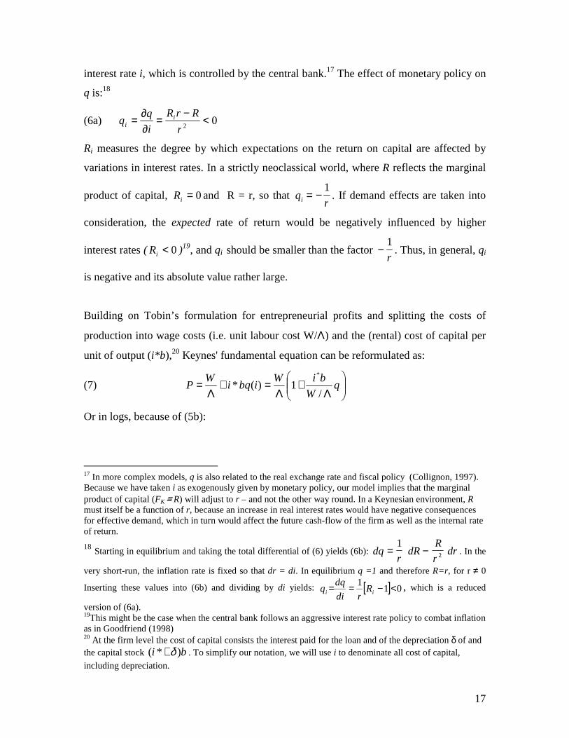
interest rate i, which is controlled by the central bank.17 The effect of monetary policy on

q is:18

(6a) 02

<−

=∂∂=

r

RrR

i

qq i

i

Ri measures the degree by which expectations on the return on capital are affected by

variations in interest rates. In a strictly neoclassical world, where R reflects the marginal

product of capital, 0=iR and R = r, so that qri = −1

. If demand effects are taken into

consideration, the expected rate of return would be negatively influenced by higher

interest rates ( 0<iR )19, and qi should be smaller than the factor −1

r. Thus, in general, qi

is negative and its absolute value rather large.

Building on Tobin’s formulation for entrepreneurial profits and splitting the costs of

production into wage costs (i.e. unit labour cost W/Λ) and the (rental) cost of capital per

unit of output (i*b ),20 Keynes' fundamental equation can be reformulated as:

(7)

Λ+

Λ=+

Λ= q

W

biWibqi

WP

/1)(*

*

Or in logs, because of (5b):

17 In more complex models, q is also related to the real exchange rate and fiscal policy (Collignon, 1997). Because we have taken i as exogenously given by monetary policy, our model implies that the marginal product of capital (FK ≡ R) will adjust to r – and not the other way round. In a Keynesian environment, R must itself be a function of r, because an increase in real interest rates would have negative consequences for effective demand, which in turn would affect the future cash-flow of the firm as well as the internal rate of return.

18 Starting in equilibrium and taking the total differential of (6) yields (6b): dqr

dRR

rdr= −

12 . In the

very short-run, the inflation rate is fixed so that dr = di. In equilibrium q =1 and therefore R=r, for r ≠ 0

Inserting these values into (6b) and dividing by di yields: [ ] 011 <−== ii Rrdi

dqq , which is a reduced

version of (6a). 19This might be the case when the central bank follows an aggressive interest rate policy to combat inflation as in Goodfriend (1998) 20 At the firm level the cost of capital consists the interest paid for the loan and of the depreciation δ of and the capital stock bi )*( δ+ . To simplify our notation, we will use i to denominate all cost of capital,

including depreciation.

18

(7’)

Λ++−=+−= q

W

biwcwp

/1ln

*

λλ

We have now a theory for the mark up. Prices are determined by unit labour costs and the

mark-up, which covers the cost of capital and entrepreneurial profits. The value of capital

equipment purchased is equal to the value of loans (P0K=B) and b is the ratio of

outstanding loans (B) to output (Y) or the historic value of capital per unit of output.

The mark-up is determined by the cost of capital and the margin of entrepreneurial

profits, given unit labour costs. From (6) we know that when the actual return on capital

is equal to the required return i* , there are no entrepreneurial profits: 1*)()( == iqiq .

The market value of the investment project is then equal to its replacement costs and its

net present value is zero. This condition reflects therefore the "normal" or equilibrium

capacity utilisation of the firm and *i represents Wicksell’s “natural rate of interest”,

which determines also the natural rate of unemployment. But, as Woodford (2003:20)

rightly points out, various types of real disturbance can create temporary fluctuations in

the “natural rate of interest” and the level of nominal interest rates required to stabilise

both inflation and output varies over time.

The equilibrium price level (P*) is determined by unit labour costs (W/Λ) and the

“normal” cost of capital per output.

(7a) biW

P ** +Λ

= or in logs ** Tcwp +−= λ

where )/

*1(ln*

Λ+=

W

bicT

Because *i is the required rate of return, cT * is the minimum mark-up, which firms need

to target in order to service their debt liabilities. This explains why the mark-up is set as

the exogenous variable in our system by the capital market and, more precisely, by

monetary policy. Firms must set prices so that they cover their cost of capital, and the

labour market will have to adjust. However, note that q may also drive a wedge between

the actual and the required mark up, if entrepreneurial profits are positive or negative.

19

This wedge is transitory, but has long-term effects for the level of the capital stock and

may therefore explain shifts in the Phillips curve.

The mark-up and interest rates

How does monetary policy affect inflation and the mark-up? Taking first differences of

(5b) yields the inflation rate. Usingµµd

c =∆ , where Λ

=/

*

W

bqiµ we get the elasticity by

which the mark-up responds to an interest variation:

(7c) 0)1(1

*

*

<−+=∂∂=

∂∂=

i

q

q

qi

ii

c i φµ

µβ

We call β the transmission coefficient and write the inflation equation:21

(8) iwp ∆+∆−∆=∆ βλ)(

Inflation is determined by unit labour cost increases and monetary policy. An interest rate

hike i∆ operates through two channels: (i) because 0<iq , it reduces demand and actual

prices. But if interest rates are flexible, it also increases capital costs. On balance, a rise in

rates by the central bank will lower inflation, if the demand effect dominates the cost

effect. We assume that this is generally the case, so that β < 0. 22 (ii) However, the larger

the share of flexible rates in the economy, the larger will be the cost effect and the lower

will be the transmission coefficient β, by which inflation responds to monetary policy.

Thus, financial structure matters for the transmission of monetary policy. As long as there

are some flexible rate credit contracts, a rate hike also increases the required mark-up *Tc

needed for firms to service their debt. Thus, the total change in the targeted mark-up is:

(5e) 0* <∆+∆=∆ ββ foricc TT

If all loans were fixed rate contracts, 0* =Tc∆ and monetary policy would only affect

profits, but not capital cost. Firms will then only target an increase in the mark-up to

recuperate the demand induced losses, but not higher costs of capital. In any case, a rising

interest rates (∆i) will depress effective demand, because qi < 0. The price level and

actual mark-up then fall below their expected equilibrium level (p < p*). To service their

21 The coefficient φ reflects the share of fixed interest rate bonds in the aggregate credit volume. See

Collignon, 2002 for details. 1=φ implies that all loans carry fixed interest rates. 22 For a formal derivation of this statement see Collignon, 2002.

20

debt, firms have to target higher mark-ups, causing higher unemployment. If profit

margins respond with high elasticity to changes in employment, while adjustment costs

and uncertainty will cause the capital stock to adjust only slowly, disequilibrium

unemployment will be high. But if the demand-induced fall of actual mark-ups below

equilibrium levels leads to a reduction in the capital stock, the labour demand curve will

shift to the left until the mark-up has attained the level necessary to service capital. See

figure 2. The equilibrium rate of unemployment will have risen as a consequence of a

persistent23 one-off increase in interest rates.24 The opposite movement occurs when the

central bank cuts interest rates. Thus, by setting the marginal interest rate, the central

bank determines the required mark-up and monetary policy has long run real effects.

Determining the capital stock

The capital market is the place where changes in monetary policy will translate into

adjustment of the capital stock. The capital market is in equilibrium when investment

neither increases nor decreases.25 At this point the labour market also is in equilibrium.

The adjustment can be modelled by using Tobin’s investment function. In the long run

firms will expand their productive capacity if the rate of return from investment exceeds

the cost of capital. If the return is less, firms go bankrupt and the capital stock is

reduced.26 In neo-classical models, R is equivalent to the marginal product of capital (FK),

a technical variable dependent on the size of the capital stock. Investment is determined

by the growth of the capital stock to the point where the marginal product of capital (FK ≡

R) is equal to r. Thus, entrepreneurial profits tend to disappear as the capital stock

increases. When the capital stock is in equilibrium, all opportunities for entrepreneurial

profits have been exhausted and the return on capital reflects the costs of borrowing, so

that Tobin’s q( *)i =1 . Hence, there are an infinite number of natural rates of interest and

unemployment.

23 A persistent change in interest rates is defined as a rate variation that lasts until the capital stock has adjusted. 24 For a model explaining the NAIRU as an autoregressive process with hysteresis see Taheri, 2000 25 This is Wicksell’s natural rate, where planned savings are equal to planned investment (Wicksell, 1965:xiii). 26 Investment may already stop at an earlier rate, say q , if a minimum profit rate is required for investment.

See Collignon, 2002.

21

The speed of convergence to equilibrium after a shock to q depends on the cost of

adjustment: if these costs were zero, the capital stock would instantaneously jump to

equilibrium where 1*)( =iq . As long as adjustment costs are positive, q will only

gradually return to 1.

The rate of investment can be modelled as a function of Tobin's q (Tobin and Brainard,

1997):

(9) [ ]*)()(0 iqiqadK −+= ϕ

In a neoclassical model, autonomous investment grows at the rate of the labour force.

Investment is stimulated if mark ups exceed the cost of capital, so that entrepreneurial

profits are positive and 1)( >iq . Monetary policy can therefore stimulate investment by

cutting the interest rate. Excess demand will then push the price level above the

equilibrium P*. But Q-profits are only temporary. They last until additional output

satisfies excess demand and the capital stock finds its new equilibrium ).1)(( == qiq At

that point the price level will also have returned to P*. Keynes’ price equation (7) implies

that profit margins at first rise above equilibrium because q >1, but fall subsequently

when competition and additional supply push q back to equilibrium. Hence, the demand-

induced acceleration of inflation is transitory - unless it spills over into wage

bargaining.27

Thus, monetary policy affects prices in the short-run (via demand iq , and via the

borrowing costs i* ), and output and employment in the long-run (via investment). But

while the impact ceases once q has returned to the level of *)(iq , the consequences are

durable. Because the capital stock has grown (or fallen) during the entire adjustment

period, the effects of a persistent interest variation are transitory on investment, but

permanent on the capital stock, employment and equilibrium output. The short-term non-

neutrality of money has long run effects.

27 To the degree that the rate cut lowers the cost of capital, the equilibrium price level P* also falls.

22

This implies, on the other hand, that the hypothesis of long run neutrality of money only

holds if interest rate variations are not persistent. In other words, the long-term neutrality

of money implies that real interest rates are stationary, meaning that although

fluctuating, they revert to a constant mean. This may be true in the very long run, but

hardly over the period, which is necessary for the capital stock to adjust to changes in

interest rates. If shocks to the interest rate exhibit variations in the mean or are highly

persistent, i.e. if their time series have a constant trend or a unit root or are close to a unit

root, monetary policy is not neutral. In fact, the very concept of monetary policy, i.e. of a

sequence of decision rules followed by the Central Bank, implies that today’s variation of

interest rates are not independent from previous ones. Only over the very long may

decisions to raise and to lower interest rates balance out. Thus, for realistic time frames in

real life, it is reasonable to give up the hypothesis of long run monetary neutrality.28

However, the degree to which monetary policy has real effects depends on real wage

rigidity, adjustments coats of investment and the financial structure of the economy.

II. Empirical Evidence for Non-Neutrality of Money

We will now look at empirical evidence for long run effects from monetary policy on

investment and employment. We will first discuss our data, then evaluate Tobin's

investment function and finally estimate our modified Phillips curve.

The data

In this section, I will give an overview of some relevant data that throw light on our

theoretical argument. We will use available data for 15 OECD industrialized countries,

most of them being members of the Euro area today. Unless indicated differently, I use

28 Breedon et alt (1999) found that real interest rates in leading developed countries for the 1967-1988 period do not appear to be stationary. Empirical findings by Karanassou et al. (2003), Henry et al. (2000), Haldane and Quah (1999) found an apparent stability of the natural rate and the Phillips curve in the very long-run, and the very prolonged after-effects of persistent shocks and structural shifts in the medium term. My reading would be that in the very long-run interest shocks are i.i.d. with zero mean, while in the medium term persistency in interest rates causes shifts in the natural rate.

23

the annual data set provided by the European Commission's AMECO. The relevant codes

are shown in appendix 1.

Interest rates

We have argued that long-term neutrality of money implies stationarity of real interest

rates. Figure 3 shows monthly short-term real interests for the USA.29 We clearly

distinguish periods of monetary turbulence in the late 1930s and 40s and in the 1970s.

Figure 3. USA: 3-month Treasury Bills, CPI inflation and Real Interest Rates

-20

-15

-10

-5

0

5

10

15

20

Jan-

34

Jan-

36

Jan-

38

Jan-

40

Jan-

42

Jan-

44

Jan-

46

Jan-

48

Jan-

50

Jan-

52

Jan-

54

Jan-

56

Jan-

58

Jan-

60

Jan-

62

Jan-

64

Jan-

66

Jan-

68

Jan-

70

Jan-

72

Jan-

74

Jan-

76

Jan-

78

Jan-

80

Jan-

82

Jan-

84

Jan-

86

Jan-

88

Jan-

90

Jan-

92

Jan-

94

Jan-

96

Jan-

98

Jan-

00

Jan-

02

Jan-

04

Jan-

06

inflation pa 3-Month Treasury Bill: Secondary Market Rate Real rate

Table 1 shows the unit root tests for some selected periods. It rejects the hypothesis of a

unit root for the very long run, but less convincingly, or not at all, for shorter periods.

Furthermore, the autoregressive coefficient in the ADF test is close to zero, indicating

long persistence in the mean reverting dynamics. For example, a coefficient of -0.029

means that only 2.9% of a real interest rate deviation from the long-term mean is

29 Data for this time series are obtained from the Federal Reserve Bank of St. Louis Economic Data (http://research.stlouisfed.org/fred2/). Inflation is calculated from Consumer Price Index for All Urban Consumers: All Items, nominal short term interest rates are: Series: TB3MS, 3-Month Treasury Bill: Secondary Market Rate.

24

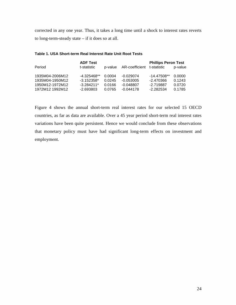
corrected in any one year. Thus, it takes a long time until a shock to interest rates reverts

to long-term-steady state – if it does so at all.

Table 1. USA Short-term Real Interest Rate Unit Roo t Tests ADF Test Phillips Peron Test Period t-statistic p-value AR-coefficient t-statistic p-value 1935M04-2006M12 -4.325468** 0.0004 -0.029074 -14.47508** 0.0000 1935M04-1950M12 -3.152358* 0.0245 -0.053005 -2.470366 0.1243 1950M12-1972M12 -3.284211* 0.0166 -0.048807 -2.719887 0.0720 1972M12 1992M12 -2.693803 0.0765 -0.044178 -2.282534 0.1785

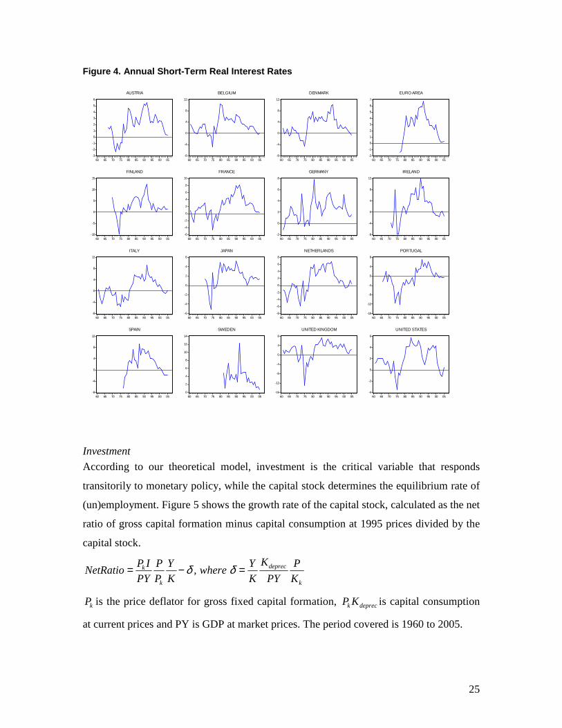
Figure 4 shows the annual short-term real interest rates for our selected 15 OECD

countries, as far as data are available. Over a 45 year period short-term real interest rates

variations have been quite persistent. Hence we would conclude from these observations

that monetary policy must have had significant long-term effects on investment and

employment.

25

Figure 4. Annual Short-Term Real Interest Rates

-3

-2

-1

0

1

2

3

4

5

6

60 65 70 75 80 85 90 95 00 05

AUSTRIA

-8

-4

0

4

8

12

60 65 70 75 80 85 90 95 00 05

BELGIUM

-8

-4

0

4

8

12

60 65 70 75 80 85 90 95 00 05

DENMARK

-2

-1

0

1

2

3

4

5

6

7

60 65 70 75 80 85 90 95 00 05

EURO AREA

-10

-5

0

5

10

15

60 65 70 75 80 85 90 95 00 05

FINLAND

-6

-4

-2

0

2

4

6

8

10

60 65 70 75 80 85 90 95 00 05

FRANCE

-2

0

2

4

6

8

60 65 70 75 80 85 90 95 00 05

GERMANY

-8

-4

0

4

8

12

60 65 70 75 80 85 90 95 00 05

IRELAND

-8

-4

0

4

8

12

60 65 70 75 80 85 90 95 00 05

ITALY

-6

-4

-2

0

2

4

6

60 65 70 75 80 85 90 95 00 05

JAPAN

-8

-6

-4

-2

0

2

4

6

8

60 65 70 75 80 85 90 95 00 05

NETHERLANDS

-16

-12

-8

-4

0

4

8

60 65 70 75 80 85 90 95 00 05

PORTUGAL

-8

-4

0

4

8

12

60 65 70 75 80 85 90 95 00 05

SPAIN

0

2

4

6

8

10

12

14

60 65 70 75 80 85 90 95 00 05

SWEDEN

-16

-12

-8

-4

0

4

8

60 65 70 75 80 85 90 95 00 05

UNITED KINGDOM

-4

-2

0

2

4

6

60 65 70 75 80 85 90 95 00 05

UNITED STATES

Investment

According to our theoretical model, investment is the critical variable that responds

transitorily to monetary policy, while the capital stock determines the equilibrium rate of

(un)employment. Figure 5 shows the growth rate of the capital stock, calculated as the net

ratio of gross capital formation minus capital consumption at 1995 prices divided by the

capital stock.

k

deprec

k

k

K

P

PY

K

K

Ywhere

K

Y

P

P

PY

IPNetRatio =−= δδ ,

kP is the price deflator for gross fixed capital formation, depreckKP is capital consumption

at current prices and PY is GDP at market prices. The period covered is 1960 to 2005.

26

We are interested in the long-term effects of short-term variations, assuming that the

long-term trend of investment may follow more fundamental factors like population

growth, structural changes in the world economy etc. The long-term trend has been

calculated by applying the Hodrick-Prescott Filter (with lambda=100) to the data. Figure

5 shows the results, as well as the short-term cyclical deviations from the long-term trend.

We observe a marked reduction in long-term investment trend in all countries. It has

fallen to remarkable low levels in France, Germany, Japan, Belgium and the Netherlands

and less so in the USA, UK, Ireland, Spain and Portugal. The cyclical variations around

the trend oscillate with a margin of plus/minus 10%. For the sake of this paper, we are

not interested in the explanation of the trend, but in the long-term effects of the short-

term cyclical variations. The long-term effects on the investment rate will depend on a

number of other factors, which we do not discuss in this paper, notable, the role of fiscal

policy and public investment or globalisation (see Collignon, 2008 – forthcoming).

27

Figure 5. Investment growth

-.010

-.005

.000

.005

.010

.01

.02

.03

.04

.05

.06

60 65 70 75 80 85 90 95 00 05

NetRatio Trend Cycle

France

-.015

-.010

-.005

.000

.005

.010

.00

.02

.04

.06

.08

60 65 70 75 80 85 90 95 00 05

NetRatio Trend Cycle

Germany

-.015

-.010

-.005

.000

.005

.010

.01

.02

.03

.04

.05

60 65 70 75 80 85 90 95 00 05

NetRatio Trend Cycle

United States

-.010

-.005

.000

.005

.010

.015

.00

.01

.02

.03

.04

60 65 70 75 80 85 90 95 00 05

NetRatio Trend Cycle

United Kingdom

-.02

-.01

.00

.01

.02

.03

.00

.04

.08

.12

60 65 70 75 80 85 90 95 00 05

NetRatio Trend Cycle

Japan

-.015

-.010

-.005

.000

.005

.010

.015

.01

.02

.03

.04

.05

.06

.07

60 65 70 75 80 85 90 95 00 05

NetRatio Trend Cycle

Italy

-.015

-.010

-.005

.000

.005

.010

.02

.03

.04

.05

.06

.07

60 65 70 75 80 85 90 95 00 05

NetRatio Trend Cycle

Austria

-.015

-.010

-.005

.000

.005

.010

.015

.00

.01

.02

.03

.04

.05

60 65 70 75 80 85 90 95 00 05

NetRatio Trend Cycle

Belgium

-.02

-.01

.00

.01

.02

.00

.01

.02

.03

.04

.05

.06

60 65 70 75 80 85 90 95 00 05

NetRatio Trend Cycle

Denmark

Tobin’s q

From a theoretical point of view, Tobin’s investment function describes the dynamics of

investment behaviour as a function of q adequately. Empirical work, however, has

encountered difficulties since the early 1990s. This may be due to the statistical indicators

used in such work. Tobin defined q in terms of “the ratio of the market valuations of

capital assets to their replacement costs, for example the prices of existing houses relative

to costs of building comparable new ones. For corporate business the market valuations

are made in the securities markets” (Tobin, 1986). Subsequently many researchers used

the ratio of a country’s stock exchange to the producer price index as an indicator for

28

Tobin’s q. Figure 6 gives the example of a number of US as well as the UK industrial

share price indeces.30

Figure 6. Share price index deflated by producer pric es: USA and UK

0

0.2

0.4

0.6

0.8

1

1.2

1.4

1.6

1.8

2

Q11957

Q31959

Q11962

Q31964

Q11967

Q31969

Q11972

Q31974

Q11977

Q31979

Q11982

Q31984

Q11987

Q31989

Q11992

Q31994

Q11997

Q31999

Q12002

Q32004

SHARE PRICES NASDAQ COMPOSITE S&P INDUSTRIALS AMEX AVERAGE UK industrial share prices

It is immediately obvious and confirmed by formal unit root tests that these indicators are

not stationary, contrary to what q-theory would lead us to expect. Especially in the early

1990 a rapid acceleration occurs, which has made these indicators useless as a proxy for

Tobin’s q. The reason is probably that economic liberalisation and globalisation have

benefited large publicly quoted companies in the tradable sector, while small businesses

especially in the non-tradable sector are lacking behind, so that a deflated share price

index would be a distorted proxy for Tobin’s q. I therefore propose to derive empirical

indicators for Tobin’s q from equation (6), using the AMECO data base for

macroeconomic variables. Our formula is:

YKPi

Pq

k

w

/)(

)1(

δσ

+−= , where P stands for the GDP deflator, wσ for the wage share, i for

nominal short-term interest rates, δ for the depreciation rate, Pk the price deflator for

gross fixed capital formation and K/Y the capital-output ratio or the inverse of capital

productivity. Hence q is the ratio of profits per output to the cost of capital per output.

Figure 7 shows the results.

30 Source: IMF International Financial Statistics

29

Figure 7. Tobin’s q in some selected OECD countries 31

-.4

-.2

.0

.2

.4

0.4

0.8

1.2

1.6

2.0

2.4

60 65 70 75 80 85 90 95 00 05

Q Trend Cycle

France

-.6

-.4

-.2

.0

.2

.4

.6

0.4

0.8

1.2

1.6

2.0

2.4

60 65 70 75 80 85 90 95 00 05

Q Trend Cycle

Germany

-.4

-.2

.0

.2

.4

.6

0.4

0.8

1.2

1.6

2.0

2.4

60 65 70 75 80 85 90 95 00 05

Q Trend Cycle

United States

-.3

-.2

-.1

.0

.1

.2

.3

0.4

0.8

1.2

1.6

2.0

2.4

60 65 70 75 80 85 90 95 00 05

Q Trend Cycle

United Kingdom

-.4

-.2

.0

.2

.4

0.4

0.8

1.2

1.6

2.0

2.4

60 65 70 75 80 85 90 95 00 05

Q Trend Cycle

Japan

-.4

-.2

.0

.2

.4

.6

0.4

0.8

1.2

1.6

2.0

2.4

60 65 70 75 80 85 90 95 00 05

Q Trend Cycle

Italy

-.4

-.2

.0

.2

.4

0.4

0.8

1.2

1.6

2.0

2.4

60 65 70 75 80 85 90 95 00 05

Q Trend Cycle

Austria

-.4

-.2

.0

.2

.4

0.4

0.8

1.2

1.6

2.0

2.4

60 65 70 75 80 85 90 95 00 05

Q Trend Cycle

Belgium

-.4

-.2

.0

.2

.4

0.4

0.8

1.2

1.6

2.0

2.4

60 65 70 75 80 85 90 95 00 05

Q Trend Cycle

Finland

-.3

-.2

-.1

.0

.1

.2

.3

0.4

0.8

1.2

1.6

2.0

2.4

60 65 70 75 80 85 90 95 00 05

Q Trend Cycle

Denmark

-.4

-.2

.0

.2

.4

.6

0.4

0.8

1.2

1.6

2.0

2.4

60 65 70 75 80 85 90 95 00 05

Q Trend Cycle

Portugal

-.2

-.1

.0

.1

.2

.3

.4

0.4

0.8

1.2

1.6

2.0

2.4

60 65 70 75 80 85 90 95 00 05

Q Trend Cycle

Spain

These data seem more consistent with theory. Although they, too, show a clear

improvement in entrepreneurial profits after 1992, the rapid growth in entrepreneurial

profits at the end of the period now simply appears as a return to levels that prevailed in

the early 1960. However, our time series is too short to assume stationarity. We have

31 Eview’s software has transformed small q into Q.

30

therefore detrended the series by the Hodrick-Prescott filter and use the trend deviations

as the policy proxy, which reflects monetary policy. Note also, that by construction, our

measure for q is dependant on interest rates. An increase in interest rates lowers q. We

have calculated our q by using short-term nominal rates, as they are under the control of

monetary authorities. We will now estimate how such shocks to Tobin’s q have affected

investment and the level of the capital stock.

The long-term effects of short-term variation in Tobin’s q

We have argued that if monetary policy can affect Tobin’s q, it will have a long-term

impact on the capital stock, which in return determines the demand for labour and

therefore equilibrium unemployment. We will now look at the long-term adjustment

process of the capital stock. In the next section we will then analyse short-term

adjustment in the labour market.

The VAR model

We obtain evidence for long run effects from estimating a Vector Autoregression (VAR)

relating transitory shocks from Tobin’s q to the growth rate of investment. The cumulated

effects of such shocks determine the long run evolution of the capital stock and therefore

of equilibrium employment. The VAR consists of two variables: q and NetRatio (the ratio

of net investment to the capital stock). As mentioned, the series were not stationary; we

therefore detrended the variables by applying the HP-filter. The VAR can be written as

follows:

tqtqtt CYAYAY ζ+++= −− ...11

Where C is a 2×2 upper triangular matrix with diagonal terms equal to unity, and tζ is a

2-dimensional vector of zero-mean, serially uncorrelated shocks with diagonal variance-

covariance matrix. This means that q responds contemporaneously to shocks in NetRatio,

but investment doesn't respond contemporaneously to a shock in q. The lag length of the

VAR was chosen based on the Likelihood Ratio test. Since the series were detrended

with the HP-Filter, their mean is zero, so no constant was used for efficiency purposes.

31

The coefficients of A1... Aq, C and the variances of each element tζ , where estimated

using Ordinary Least Squares. All details can be found in the appendix.

Results

Our objective is to determine the path of NetRatio after a one-standard-deviation shock in

q and its cumulative effect, as well as the response of q after a one-standard-deviation

shock in NetRatio. According to our theoretical model, we would expect short-term non-

neutrality, but long-term neutrality of q-shocks on investment; short-term variations in

investment accumulate to long-term changes in the capital stock. As the capital stock

increases, extra profits are eliminated and q is returning to its equilibrium value. Figure 8

shows the results.

32

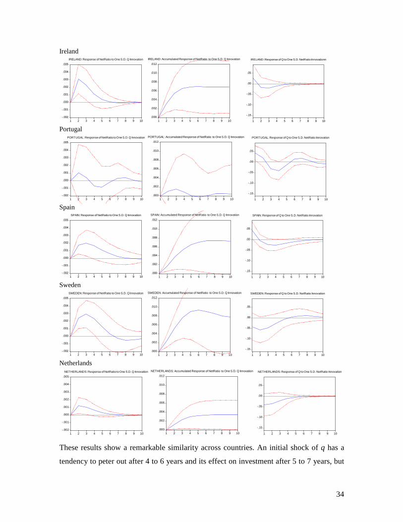
Figure 8. The Impact of short-term variations of To bin’s q on investment and capital

France

-.002

-.001

.000

.001

.002

.003

.004

.005

1 2 3 4 5 6 7 8 9 10

FRANCE: Response of NetRatio to One S.D. Q Innovation

.000

.002

.004

.006

.008

.010

.012

1 2 3 4 5 6 7 8 9 10

FRANCE: Accumulated Response of NetRatio to One S.D. Q Innovation

-.15

-.10

-.05

.00

.05

1 2 3 4 5 6 7 8 9 10

FRANCE: Response of Q to One S.D. NetRatio Innovation

Germany

-.002

-.001

.000

.001

.002

.003

.004

.005

1 2 3 4 5 6 7 8 9 10

GERMANY: Response of NetRatio to One S.D. Q Innovation

.000

.002

.004

.006

.008

.010

.012

1 2 3 4 5 6 7 8 9 10

GERMANY: Accumulated Response of NetRatio to One S.D. Q Innovation

-.15

-.10

-.05

.00

.05

1 2 3 4 5 6 7 8 9 10

GERMANY: Response of Q to One S.D. NetRatio Innovation

US

-.002

-.001

.000

.001

.002

.003

.004

.005

1 2 3 4 5 6 7 8 9 10

US: Response of NetRatio to One S.D. Q Innovation

.000

.002

.004

.006

.008

.010

.012

1 2 3 4 5 6 7 8 9 10

US: Accumulated Response of NetRatio to One S.D. Q Innovation

-.15

-.10

-.05

.00

.05

1 2 3 4 5 6 7 8 9 10

US: Response of Q to One S.D. NetRatio Innovation

UK

-.002

-.001

.000

.001

.002

.003

.004

.005

1 2 3 4 5 6 7 8 9 10

UK: Response of NetRatio to One S.D. Q Innovation

.000

.002

.004

.006

.008

.010

.012

1 2 3 4 5 6 7 8 9 10

UK: Accumulated Response of NetRatio to One S.D. Q Innovation

-.15

-.10

-.05

.00

.05

1 2 3 4 5 6 7 8 9 10

UK: Response of Q to One S.D. NetRatio Innovation

Japan

-.002

-.001

.000

.001

.002

.003

.004

.005

1 2 3 4 5 6 7 8 9 10

JAPAN: Response of NetRatio to One S.D. Q Innovation

.000

.002

.004

.006

.008

.010

.012

1 2 3 4 5 6 7 8 9 10

JAPAN: Accumulated Response of NetRatio to One S.D. Q Innovation

-.15

-.10

-.05

.00

.05

1 2 3 4 5 6 7 8 9 10

JAPAN: Response of Q to One S.D. NetRatio Innovation

33

Italy

-.002

-.001

.000

.001

.002

.003

.004

.005

1 2 3 4 5 6 7 8 9 10

ITALY: Response of NetRatio to One S.D. Q Innovation

.000

.002

.004

.006

.008

.010

.012

1 2 3 4 5 6 7 8 9 10

ITALY: Accumulated Response of NetRatio to One S.D. Q Innovation

-.15

-.10

-.05

.00

.05

1 2 3 4 5 6 7 8 9 10

ITALY: Response of Q to One S.D. NetRatio Innovation

Austria

-.002

-.001

.000

.001

.002

.003

.004

.005

1 2 3 4 5 6 7 8 9 10

Austria: Response of NetRatio to One S.D. Q Innovation

.000

.002

.004

.006

.008

.010

.012

1 2 3 4 5 6 7 8 9 10

AUSTRIA: Accumulated Response of NetRatio to One S.D. Q Innovation

-.15

-.10

-.05

.00

.05

1 2 3 4 5 6 7 8 9 10

AUSTRIA: Response of Q to One S.D. NetRatio Innovation

Belgium

-.002

-.001

.000

.001

.002

.003

.004

.005

1 2 3 4 5 6 7 8 9 10

BELGIUM: Response of NetRatio to One S.D. Q Innovation

.000

.002

.004

.006

.008

.010

.012

1 2 3 4 5 6 7 8 9 10

BELGIUM: Accumulated Response of NetRatio to One S.D. Q Innovation

-.15

-.10

-.05

.00

.05

1 2 3 4 5 6 7 8 9 10

BELGIUM: Response of Q to One S.D. NetRatio Innovation

Denmark

-.002

-.001

.000

.001

.002

.003

.004

.005

1 2 3 4 5 6 7 8 9 10

DENMARK: Response of NetRatio to One S.D. Q Innovation

.000

.002

.004

.006

.008

.010

.012

1 2 3 4 5 6 7 8 9 10

DENMARK: Accumulated Response of NetRatio to One S.D. Q Innovation

-.15

-.10

-.05

.00

.05

1 2 3 4 5 6 7 8 9 10

DENMARK: Response of Q to One S.D. NetRatio Innovation

Finland

-.002

-.001

.000

.001

.002

.003

.004

.005

1 2 3 4 5 6 7 8 9 10

FINLAND: Response of NetRatio to One S.D. Q Innovation

.000

.002

.004

.006

.008

.010

.012

1 2 3 4 5 6 7 8 9 10

FINLAND: Accumulated Response of NetRatio to One S.D. Q Innovation

-.15

-.10

-.05

.00

.05

1 2 3 4 5 6 7 8 9 10

FINLAND: Response of Q to One S.D. NetRatio Innovation

34

Ireland

-.002

-.001

.000

.001

.002

.003

.004

.005

1 2 3 4 5 6 7 8 9 10

IRELAND: Response of NetRatio to One S.D. Q Innovation

.000

.002

.004

.006

.008

.010

.012

1 2 3 4 5 6 7 8 9 10

IRELAND: Accumulated Response of NetRatio to One S.D. Q Innovation

-.15

-.10

-.05

.00

.05

1 2 3 4 5 6 7 8 9 10

IRELAND: Response of Q to One S.D. NetRatio Innovationn

Portugal

-.002

-.001

.000

.001

.002

.003

.004

.005

1 2 3 4 5 6 7 8 9 10

PORTUGAL: Response of NetRatio to One S.D. Q Innovation

.000

.002

.004

.006

.008

.010

.012

1 2 3 4 5 6 7 8 9 10

PORTUGAL: Accumulated Response of NetRatio to One S.D. Q Innovation

-.15

-.10

-.05

.00

.05

1 2 3 4 5 6 7 8 9 10

PORTUGAL: Response of Q to One S.D. NetRatio Innovation

Spain

-.002

-.001

.000

.001

.002

.003

.004

.005

1 2 3 4 5 6 7 8 9 10

SPAIN: Response of NetRatio to One S.D. Q Innovation

.000

.002

.004

.006

.008

.010

.012

1 2 3 4 5 6 7 8 9 10

SPAIN: Accumulated Response of NetRatio to One S.D. Q Innovation

-.15

-.10

-.05

.00

.05

1 2 3 4 5 6 7 8 9 10

SPAIN: Response of Q to One S.D. NetRatio Innovation

Sweden

-.002

-.001

.000

.001

.002

.003

.004

.005

1 2 3 4 5 6 7 8 9 10

SWEDEN: Response of NetRatio to One S.D. Q Innovation

.000

.002

.004

.006

.008

.010

.012

1 2 3 4 5 6 7 8 9 10

SWEDEN: Accumulated Response of NetRatio to One S.D. Q Innovation

-.15

-.10

-.05

.00

.05

1 2 3 4 5 6 7 8 9 10

SWEDEN: Response of Q to One S.D. NetRatio Innovation

Netherlands

-.002

-.001

.000

.001

.002

.003

.004

.005

1 2 3 4 5 6 7 8 9 10

NETHERLANDS: Response of NetRatio to One S.D. Q Innovation

.000

.002

.004

.006

.008

.010

.012

1 2 3 4 5 6 7 8 9 10

NETHERLANDS: Accumulated Response of NetRatio to One S.D. Q Innovation

-.15

-.10

-.05

.00

.05

1 2 3 4 5 6 7 8 9 10

NETHERLANDS: Response of Q to One S.D. NetRatio Innovation

These results show a remarkable similarity across countries. An initial shock of q has a

tendency to peter out after 4 to 6 years and its effect on investment after 5 to 7 years, but

35

the cumulative effect on the capital stock is in all cases positive. The only exception is

Portugal, where the results cannot be judged as significant. In most countries the effect of

a positive shock of one standard deviation of q will raise the aggregate capital stock by

about one half of a percentage point. Therefore monetary policy will have long-term

consequences for employment, even if its effect on investment is only transitory.

Estimating the modified Phillips curve

We will now discuss short-term Phillips curve dynamics. We are interested to find out

how employment will respond to a change in the targeted mark up. There are two

mechanisms of adjustment. In the long run, the Phillips curve will shift horizontally with

the capital stock; in the short run movements can take place along the Phillips curve.

One explanation may be economic uncertainty. For example, if interest rate variations are

volatile, the profit shares to be targeted by price setters are uncertain and investment may

not respond strongly (Dixit and Pindyck, 1994). However, firms may still need to adjust

employment to the changed profit environment in order to service their debt.

The ARMA model

In order to find the short run movements on the Phillips curve, we estimate the following

ARMA(p,q) model:

tttt udsaInvestdaaLd +++= 210 lnln

qtqttptpttt uuuu −−−−− +++++++= εθεθερρρ ...... 112211

Where ln stands for a log variable, d is the first difference of the time variable, L is

employment, s is the log of the profit share and Invest is gross investment. We regress

the growth rate of employment on the rate of investment growth and the percentage rate

of change of the profit share. We take employment growth as a proxy for excess demand

for labour, which is justified by introducing the constant 0a , We also use the growth rate

of investment, rather than the capital stock, as the latter is a I(2) time series. Testing for

36

unit roots confirmed that all variables are stationary.32 The coefficient 2a in our

regression is a measure of the inverse of the slope of the modified Phillips curve.

The results

The AR(p) is the autoregressive term in the unconditional residual, MA(q) is its moving

average representation. In order to establish the true structure of the residuals in the

ARMA(p,q) process, we first OLS-regressed the employment growth rate on the two

explanatory variables without lags and then tested the residuals for stationarity and white

noise for each of the 14 countries. After this preliminary work we determined the

possible ARMA form of the residuals using the autocorrelograms (normal for q, partial

for p), and then checked for the significance of the higher order coefficients of the

ARMA estimation. At last, we regress the growth rate of employment on the rate of

investment growth and the percentage rate of change of the profit share constraining the

residual to the predetermined ARMA(p,q).33 This regression yielded the coefficients

reported in Table 2.

32 For the regressions in Table 2, we used the up-dated annual time series 1960-2008 from AMECO, published in December 2006, which include forecasts until 2008. 33 When the residual were of an AR(p) form only, we used the maximum likelihood estimation with SAS software; We used least square iterative method of Eviews in the other cases.

37

Table 2. Phillips curve estimates

constant ∆∆∆∆c: profit share growth investment growth rate Constrained residual structureDenmark 0.0003 -0.099 0.106 AR(15)s.e.[p-value] 0.001 0.055 [0.08]* 0.014*** only AR15 non zero coeff

Germany 0.002 -0.165 0.103 AR(1)s.e.[p-value] 0.002 0.065[0.0149]** 0,021***

Spain 0.001 -0.09 -0.024 ARMA(1,4)s.e.[p-value] 0.007* 0,015[0.00001]*** 0.01 only AR1,MA1,MA4 non zero coeff

France 0.003 -0.139 0.085 0.065(15,15)s.e.[p-value] 0.0009*** 0.059[0.059]* 0.013*** only AR1, AR15, MA15, MA16 non-zero

Ireland 0.008 -0.116 0.115 AR(1)s.e.[p-value] 0.003** 0,066 [0.088]* 0,031***

Italy 0.007 -0.107 0.076 ARMA(1,2)s.e.[p-value] 0.001*** 0.058[0.072]* 0,025**

Netherland 0.01 -0.099 0.091 AR(1)s.e.[p-value] 0.003*** 0,007[0.177] 0,028***

Austria 0.002 -0.053 0.051 AR(1)s.e.[p-value] 0.002 0.021[0.014]** 0,014***

Portugal 0.0007 -0.052 0.051 AR(3)s.e.[p-value] 0.0002 0.017[0.004]*** 0,014***

Finland -0.0004 -0.049 0.092 AR(1)s.e.[p-value] 0.002 0.041[0.24] 0,02*

Sweden 0.002 -0.106 0.092 AR(14)s.e.[p-value] 0.001 0.05[0.044]** 0,02***

UK 0.001 -0.136 0.093 AR(1)s.e.[p-value] 0.002 0.047[0.005]*** 0.022***

USA 0.011 -0.259 0.140 AR(1)s.e.[p-value] 0.002*** 0.059[<0.0001]*** 0.015***

Japan 0.0003 -0.049 0.084 AR(1)s.e.[p-value] 0.0002 0,025[0.059]* 0,019***

For the confidence intervals: * between 5 and 10%; ** between 1 and 5%; *** less than 1 %.

The results are consistent with our theoretical model. All coefficients have the right sign,

with the exception of investment in Spain which is also statistically insignificant. The

responsiveness of employment to changes in the profit share is negative and statistically

significant in all cases except Finland. It is highest in the USA (our modified Phillips

curve is flat) and rather large in Germany, France and UK; it is small (the modified

Phillips curve is steep) in Austria, Portugal, Finland and Japan. Thus, short-term

monetary shocks are likely to have larger effects on disequilibrium unemployment in the

bigger OECD countries (except Japan). In a typical country like Italy or the Netherlands,

38

a 10 % increase in the required profit share would lower the growth rate of employment

by 1 percentage-point, thereby wiping out the autonomous growth of investment.

Similarly, a reduction in the growth rate of investment by one percentage-point would

also cause stagnation in employment. These are non-trivial numbers. Of course, once the

transitory effects have ceased, autonomous growth resumes, but from a lower equilibrium

level of employment and permanently increased equilibrium unemployment. On the other

hand, a sequence of interest rate cuts will have the opposite effect, raising the capital

stock and lower the NAIRU.

Conclusion

This paper has argued that the validity of long-term neutrality of money hypothesis

required that real interest rates are stationary. Empirically this seems to be only the case

over very long time periods. Over the span of several decades, monetary policy can be

non-neutral. The mechanism through which the setting of interest rates affects real

economic variables such as output and employment is Tobin’s investment function,

which models entrepreneurial profits as a function of short-term real interest rates. We

provided empirical evidence from several OECD countries that showed that the long-

term effect of an interest rate induced increase in the ratio of the return on capital to the

cost of capital will permanently increase the stock of capital and therefore output and

employment. Short-term disequilibrium unemployment depends on Phillips curve

dynamics and seems to be larger in the big OECD countries outside Japan.

These results should stimulate further research. In particular, given that the empirical

estimates are based on annual data, it would be interesting to test the long-term neutrality

hypothesis of money with higher frequency data.

28.2.2007

39

Bibliography

• Ball, L. and S. Cecchetti (1988), Imperfect Information and Staggered Price

Setting; American Economic Review 78: pp. 999-1018

• Barro, R.J. 1995. "Inflation and Economic growth." Bank of England Quaterly

Bulletin, May: 39-52.

• Blanchard, O. and Fischer, S. (1989), Lectures on Macroeconomics. Cambridge,

MIT

• Breedon F., Henry B. and Williams, G. (1999), Long-Term Real Interest Rates:

Evidence on the Golbal Capital Market. Oxford Review of Economic policy, Vol.

15.2: 128-142

• Bullard, J. and J.W. Keating. 1995. "The Long-Run Relationship between

Inflation and Output in Post-war Economies." In: Journal of Monetary

Economics, 36.3 (Dec): 477-496.

• Carlin, W. and Soskice, D. (1990), Macroeconomics and the Wage Bargain. A

Modern Approach to Employment, Inflation and the Exchange Rate. Oxford

University Press, New York.

• Collignon, S. (1997), Unemployment and Monetary Policy in the Single Market:

A Dialogue with Franco Modigliani; in: S. Collignon (ed.): European Monetary

Policy; Pinters Publishers, London.

• Collignon, S. (1999), Unemployment, Wage Developments and the European

Policy Mix in Europe ; in : Empirica, 26 :259-269

• Collignon, S. (2002), Monetary Stability in Europe. Routledge, London.

• Collignon, S. (2008) Why Europe is Not Becoming the World’s Most Dynamic

Economy, – Forthcoming in Spring 2008 in International Journal Of Public

Policy, earlier version downloadable on

http://www.stefancollignon.de/PDF/NewLisbonStrategy_8nov.pdf

• Coricelli, I., A. Cukierman and A. Dalmazzo (2003), Monetary Institutions,

Monopolistic Competition, Unionised Labour Markets and Economic

Performance. Download: http://www.tau.ac.il/valexcuk/w_p.html

40

• Dixit, A. K. and R. Pindyck (1994), Investment under Uncertainty; Princeton

University Press, Princeton, New Jersey

• Dullien, S. (2004), The Interaction of Monetary Policy and Wage Bargaining in

the European Monetary Union. Lessons from the Endogenous Money Approach.

Palgrave Macmillan: Basingstoke.

• Fischer, S. (1977), Long-term contracts, Rational Expectations, and the Optimal

Money Supply Rule ; in : Journal of Political Economy, 85(1), pp 191-205.

• Fisher, S. 1977. "Long-term Contracts, rational expectations, and the optimal

money supply rule." In: Journal of Political Economy 85 (Feb): 1991-205.

• Fisher, M.E. and J. Seater. 1993. Long-Run Neutrality and Superneutrality in an

ARIMA Framework; AER, 83.3: 402-415

• Friedman, B. M. (1999), The Future of Monetary Policy: The Central Bank as an

Army with Only a Signal Corps?*International Finance 2:3, 1999: pp. 321–338

• Friedman, M. (1968), The Role of Monetary Policy, American Economic Review

58, no.1, March 1968, pp 1-17.

• Friedman, M. and A. J. Schwartz, (1982), Monetary Trends in the United States

and the United Kingdom. Their relation to Income, Prices and Interest Rates,

1867-1975; NBER The University of Chicago Press, Chicago

• Goodfriend, M. (1998), Acquiring and Maintaining Credibility for Low Inflation:

The US Experience, in Leiderman, L. and Svenson, L (eds.).: Inflation Target,

CEPR, 1995.

• Goodhart, Ch. (1997), Why do the Monetary Authorities Smooth Interest Rates?,

in S. Collignon (ed) European Monetary Policy. London, Pinter.

• Hahn, F. and R. Solow (1995), A Critical Essay on Modern Macroeconomic

Theory. Oxford, Blackwell.

• Haldane, A and D. Quah (1999), UK Phillips curves and monetary policy, Journal

of Economics, 44, pp 259-278.

• Henry, B., M. Karanassou and D. Snower (2000), Adjustment dynamics and the

natural rate: an account of UK unemployment, Oxford Economic Papers, 52, pp

178-203.

41

• Karanassou, M., H. Sala and D. Snower (2003), Unemployment in the European

Union: a dynamic reappraisal, Economic Modelling, 20, pp 237-273.

• Keynes, J.M. (1930). A Treatise on Money Collected Writings of John Maynard

Keynes Vol. 5, London Macmillan.

• Keynes, J.M. (1936) General Theory of Employment, Interest and Money.

Collected Writings of John Maynard Keynes, Vol. 7., London: Macmillan.

• Keynes, J.M. (1973), General Theory and After P1 Prep, Collected Writings of

John Maynard Keynes, Vol. 13 London, Macmillan.

• Kuzin, V. and S. Tober , 2004. Asymmetric Monetary Policy Effects in Germany.

Discussion Papers of DIW Berlin 397/ DIW Berlin, German Institute for

Economic Research

• Layard, R., Nickell, S. and Jackman, R., 1991, Unemployment, Macroeconomic

Performance and the Labour Market, Oxford, Oxford University Press.

• Logeay, C. and S. Tober 2003. Time-Varying NAIRU and Real Interest Rates in

the Euro Area. Enepri Working Paper No. 24

• Lucas, R.E. Jr. 1996. "Nobel Lecture: Monetary Neutrality". In: Journal of

Political Economy 104.4 (August): 661-682.

• McCandless, G.T. Jr. and W.E.Weber. 1995. "Some Money Facts". Federal

Reserve Bank of Mineapolis Quaterly Review, 19.3: 2-11.

• Myrdal, G. (1933), Der Gleichgewichtsbegriff als Instrument der

geldtheoretischen Analyse, in F. A. von Hayek (ed), Beiträge zur Geldtheorie,

Springer, Wien.

• Orphanides, A. and Solow, R.M. 1990, Money Inflation and Growth; in: B.M.

Friedman and F.H. Hahn, 1990, Handbook of Monetary Economics, Amsterdam,

North Holland.

• Patinkin, D. 1989. "Neutrality of money" in: J Eatwell et al. The new Palgrave:

Money. Macmillan Reference Books, London.

• Riese, H. (1986): Theorie der Inflation. Mohr, Tübingen.

• Riese, H. (2001), Bagehot versus Goodhart: Warum eine Zentralbank

Geschäftsbanken braucht. In: Hajo Riese, Grundlegung eines monetären

42

Keynesianismus, Ausgewählte Schriften 1964-1999, Band 1; Metropolis ,

Marburg 2001

• Sargent. T. (1971), A Note on the “Accelerationist” Controversy, Journal of

Money, Banking and Credit, 3, August, pp 50-60.

• Schmidt, K. J. W. (1995), Tobins q? Myrdals Q? Ein Fallbeispiel für den Wert

von Fremdsprachenkenntnissen; Credit und Capital, 28, pp 175-200.

• Taheri, J. (2000), On the alternative explanations of persistence of unemployment

in the OECD countries; Applied Economics, 32: 1051-1057

• Taylor, J. (1979), Staggered Wage Setting in a Macro Model, American Economic

Review 69, May.

• Tobin, J. (1986), A professional Autobiography; reprintedin James Tonin, 1996,

Essays in Economics, Volume 4, MIT Press, Cambridge, MA.

• Tobin, J. and S. Golub (1998), Money, Credit and Capital, Mc Graw-Hill, New

York.

• Tobin, J. and W. Brainard (1977), Asset Markets and the Cost of Capital, in J.

Tobin (1982), Essays in Economics: Theory and Policy. Vol. 3, MIT Press,

Cambridge, Massachusetts.

• Walsh, C.E. 1998. Monetary Theory and Policy. MIT Press, Cambridge, MA.

• Wicksell, K. (1936), Interest and Prices, A study of the causes regulating the

value of money, Reprint, 1965, Augustus M. Kelly, Bookseller, New York.

• Woodford, M. (2003), Interest and Prices. Foundations of a Theory of Monetary

Policy. Princeton University Press, Princeton, New Jersey

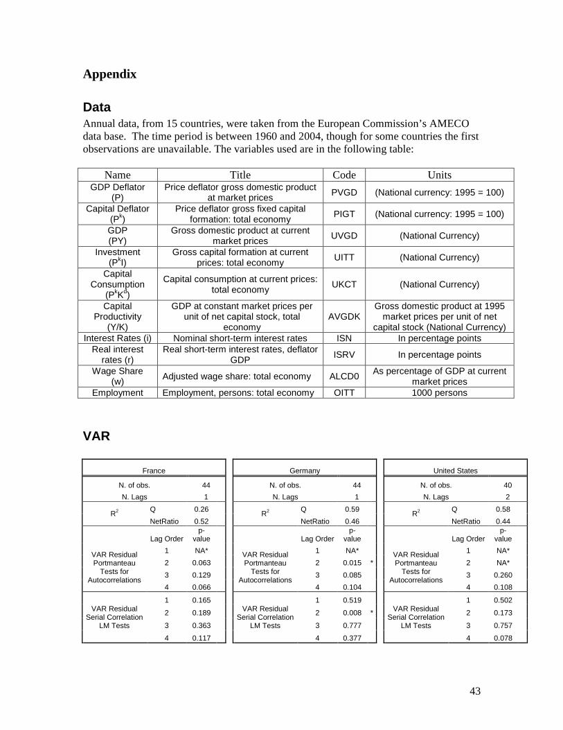
43

Appendix

Data Annual data, from 15 countries, were taken from the European Commission’s AMECO data base. The time period is between 1960 and 2004, though for some countries the first observations are unavailable. The variables used are in the following table:

Name Title Code Units GDP Deflator

(P) Price deflator gross domestic product

at market prices PVGD (National currency: 1995 = 100)

Capital Deflator (Pk)

Price deflator gross fixed capital formation: total economy

PIGT (National currency: 1995 = 100)

GDP (PY)

Gross domestic product at current market prices

UVGD (National Currency)

Investment (PkI)

Gross capital formation at current prices: total economy

UITT (National Currency)

Capital Consumption

(PkKd)

Capital consumption at current prices: total economy

UKCT (National Currency)

Capital Productivity

(Y/K)

GDP at constant market prices per unit of net capital stock, total

economy AVGDK

Gross domestic product at 1995 market prices per unit of net

capital stock (National Currency) Interest Rates (i) Nominal short-term interest rates ISN In percentage points

Real interest rates (r)

Real short-term interest rates, deflator GDP

ISRV In percentage points

Wage Share (w) Adjusted wage share: total economy ALCD0

As percentage of GDP at current market prices

Employment Employment, persons: total economy OITT 1000 persons

VAR

France Germany United States

N. of obs. 44 N. of obs. 44 N. of obs. 40

N. Lags 1 N. Lags 1 N. Lags 2

R2 Q 0.26

R2 Q 0.59

R2 Q 0.58

NetRatio 0.52 NetRatio 0.46 NetRatio 0.44

Lag Order p-

value Lag Order p-

value Lag Order p-

value

VAR Residual Portmanteau

Tests for Autocorrelations

1 NA* VAR Residual Portmanteau

Tests for Autocorrelations

1 NA* VAR Residual Portmanteau

Tests for Autocorrelations

1 NA*

2 0.063 2 0.015 * 2 NA*

3 0.129 3 0.085 3 0.260

4 0.066 4 0.104 4 0.108

VAR Residual Serial Correlation

LM Tests

1 0.165 VAR Residual

Serial Correlation LM Tests

1 0.519 VAR Residual

Serial Correlation LM Tests

1 0.502

2 0.189 2 0.008 * 2 0.173

3 0.363 3 0.777 3 0.757

4 0.117 4 0.377 4 0.078

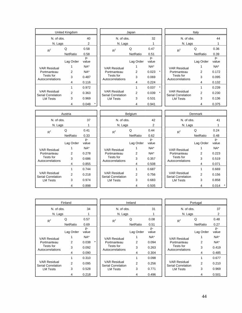
44

United Kingdom Japan Italy

N. of obs. 40 N. of obs. 32 N. of obs. 44

N. Lags 2 N. Lags 1 N. Lags 1

R2 Q 0.58

R2 Q 0.47

R2 Q 0.36

NetRatio 0.58 NetRatio 0.51 NetRatio 0.39

Lag Order p-

value Lag Order p-

value Lag Order p-

value

VAR Residual Portmanteau

Tests for Autocorrelations

1 NA* VAR Residual Portmanteau

Tests for Autocorrelations

1 NA* VAR Residual Portmanteau

Tests for Autocorrelations

1 NA*

2 NA* 2 0.023 * 2 0.172

3 0.487 3 0.069 3 0.095

4 0.116 4 0.224 4 0.132

VAR Residual Serial Correlation

LM Tests

1 0.972 VAR Residual

Serial Correlation LM Tests

1 0.037 * VAR Residual

Serial Correlation LM Tests

1 0.239

2 0.363 2 0.039 * 2 0.230

3 0.969 3 0.531 3 0.136

4 0.048 * 4 0.941 4 0.375

Austria Belgium Denmark

N. of obs. 37 N. of obs. 42 N. of obs. 41

N. Lags 1 N. Lags 2 N. Lags 1

R2 Q 0.41

R2 Q 0.44

R2 Q 0.24

NetRatio 0.33 NetRatio 0.62 NetRatio 0.48

Lag Order

p-value

Lag Order

p-value

Lag Order

p-value

VAR Residual Portmanteau

Tests for Autocorrelations

1 NA* VAR Residual Portmanteau

Tests for Autocorrelations

1 NA* VAR Residual Portmanteau

Tests for Autocorrelations

1 NA*

2 0.278 2 NA* 2 0.223

3 0.686 3 0.357 3 0.519

4 0.855 4 0.508 4 0.071

VAR Residual Serial Correlation

LM Tests

1 0.744 VAR Residual

Serial Correlation LM Tests

1 0.687 VAR Residual

Serial Correlation LM Tests

1 0.669

2 0.218 2 0.756 2 0.156

3 0.974 3 0.683 3 0.858

4 0.898 4 0.505 4 0.014 *

Finland Ireland Portugal

N. of obs. 34 N. of obs. 31 N. of obs. 37

N. Lags 1 N. Lags 1 N. Lags 2

R2 Q 0.57

R2 Q 0.08

R2 Q 0.48

NetRatio 0.69 NetRatio 0.51 NetRatio 0.27

Lag Order p-

value Lag Order p-

value Lag Order p-

value

VAR Residual Portmanteau

Tests for Autocorrelations

1 NA* VAR Residual Portmanteau

Tests for Autocorrelations

1 NA* VAR Residual Portmanteau

Tests for Autocorrelations

1 NA*

2 0.038 * 2 0.094 2 NA*

3 0.092 3 0.263 3 0.419

4 0.090 4 0.304 4 0.485

VAR Residual Serial Correlation

LM Tests

1 0.310 VAR Residual

Serial Correlation LM Tests

1 0.098 VAR Residual

Serial Correlation LM Tests

1 0.677

2 0.095 2 0.256 2 0.210

3 0.528 3 0.771 3 0.969

4 0.218 4 0.496 4 0.501

45

Spain Sweden Netherlands

N. of obs. 27 N. of obs. 20 N. of obs. 44

N. Lags 1 N. Lags 1 N. Lags 1

R2 Q 0.24

R2 Q 0.44

R2 Q 0.17

NetRatio 0.74 NetRatio 0.68 NetRatio 0.29

Lag Order p-

value Lag Order p-

value Lag Order p-

value

VAR Residual Portmanteau

Tests for Autocorrelations

1 NA* VAR Residual Portmanteau

Tests for Autocorrelations

1 NA* VAR Residual Portmanteau

Tests for Autocorrelations

1 NA*

2 0.104 2 0.178 2 0.326

3 0.221 3 0.366 3 0.463

4 0.302 4 0.313 4 0.143

VAR Residual Serial Correlation

LM Tests

1 0.583 VAR Residual

Serial Correlation LM Tests

1 0.267 VAR Residual

Serial Correlation LM Tests

1 0.242

2 0.221 2 0.646 2 0.499

3 0.651 3 0.755 3 0.599

4 0.574 4 0.104 4 0.054