The Lagrangian:Art of Smoothed Particle

Hydrodynamics

Report by Yun Fei

Nov. 2012

Introduction to Fluid MechanicsHow the story began…

Where we are

Fluid Simulation

Rendering & Materials Computational

Geometry

Hardware Computin

g

Medical ImagingSampling

Image Processing

Scientific Computing

Computational Physics

Animation

Visualize

Surface Construction

Acceleration

Flow in VesselsDensity Estimation

Better Appealing

Foundation

Numerical Methods

Motivation

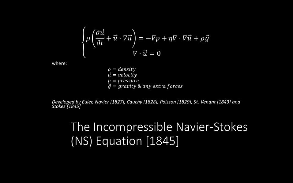
The Incompressible Navier-Stokes (NS) Equation [1845]

𝜌𝜕𝑢

𝜕𝑡+ 𝑢 ⋅ 𝛻𝑢 = −𝛻𝑝 + 𝜂𝛻 ⋅ 𝛻𝑢 + 𝜌 𝑔

𝛻 ⋅ 𝑢 = 0where:

𝜌 = 𝑑𝑒𝑛𝑠𝑖𝑡𝑦𝑢 = 𝑣𝑒𝑙𝑜𝑐𝑖𝑡𝑦𝑝 = 𝑝𝑟𝑒𝑠𝑠𝑢𝑟𝑒 𝑔 = 𝑔𝑟𝑎𝑣𝑖𝑡𝑦 & 𝑎𝑛𝑦 𝑒𝑥𝑡𝑟𝑎 𝑓𝑜𝑟𝑐𝑒𝑠

Developed by Euler, Navier [1827], Cauchy [1828], Poisson [1829], St. Venant [1843] and Stokes [1845]

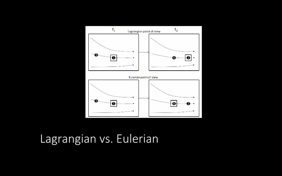
Lagrangian vs. Eulerian

From Newtonian to Navier-Stokes

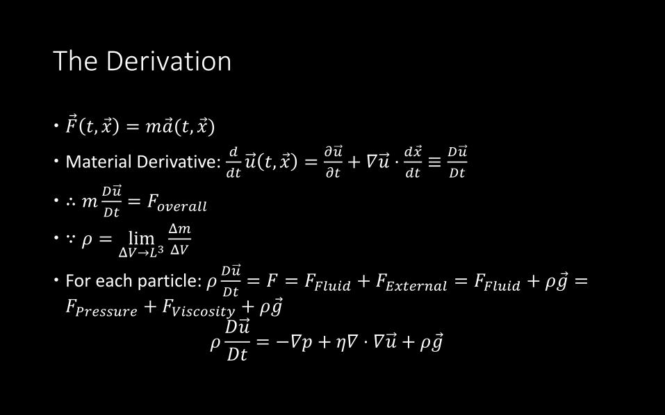
The Derivation

The Basics

Gradient: 𝛻𝑓 𝑥, 𝑦, 𝑧 =𝜕𝑓

𝜕𝑥,𝜕𝑓

𝜕𝑦,𝜕𝑓

𝜕𝑧, 𝛻 =

𝜕

𝜕𝑥,𝜕

𝜕𝑦,𝜕

𝜕𝑧

Directional Derivation: 𝜕𝑓

𝜕𝑛= 𝛻𝑓 ⋅ 𝑛

Divergence: 𝛻 ⋅ 𝑢 = 𝛻 ⋅ 𝑢, 𝑣, 𝑤 =𝜕𝑢

𝜕𝑥+𝜕𝑣

𝜕𝑦+𝜕𝑤

𝜕𝑧

Curl: 𝛻 × 𝑢 = 𝛻 × 𝑢, 𝑣,𝑤 =𝜕𝑤

𝜕𝑦−𝜕𝑣

𝜕𝑧,𝜕𝑢

𝜕𝑧−𝜕𝑤

𝜕𝑥,𝜕𝑣

𝜕𝑥−𝜕𝑢

𝜕𝑦

Laplacian: 𝛻 ⋅ 𝛻𝑓 =𝜕2𝑓

𝜕𝑥2+𝜕2𝑓

𝜕𝑦2+𝜕2𝑓

𝜕𝑧2

Poisson Equation: 𝛻 ⋅ 𝛻𝑓 = 𝑞, (for 𝑞 = 0, we call it Laplace’s Equation)

The Gauss Theorem: Ω𝛻 ⋅ 𝑢 = 𝜕Ω 𝑢 ⋅ 𝑛

The Derivation

𝐹 𝑡, 𝑥 = 𝑚 𝑎(𝑡, 𝑥)

Material Derivative: 𝑑

𝑑𝑡𝑢 𝑡, 𝑥 =

𝜕𝑢

𝜕𝑡+ 𝛻𝑢 ⋅

𝑑 𝑥

𝑑𝑡≡𝐷𝑢

𝐷𝑡

∴ 𝑚𝐷𝑢

𝐷𝑡= 𝐹𝑜𝑣𝑒𝑟𝑎𝑙𝑙

∵ 𝜌 = limΔ𝑉→𝐿3

Δ𝑚

Δ𝑉

For each particle: 𝜌𝐷𝑢

𝐷𝑡= 𝐹 = 𝐹𝐹𝑙𝑢𝑖𝑑 + 𝐹𝐸𝑥𝑡𝑒𝑟𝑛𝑎𝑙 = 𝐹𝐹𝑙𝑢𝑖𝑑 + 𝜌 𝑔 =

𝐹𝑃𝑟𝑒𝑠𝑠𝑢𝑟𝑒 + 𝐹𝑉𝑖𝑠𝑐𝑜𝑠𝑖𝑡𝑦 + 𝜌 𝑔

𝜌𝐷𝑢

𝐷𝑡= −𝛻𝑝 + 𝜂𝛻 ⋅ 𝛻𝑢 + 𝜌 𝑔

Incompressibility

For an arbitrary chunk of fluid Ω, its volume doesn’t change along time:

𝑑

𝑑𝑡𝑣𝑜𝑙𝑢𝑚𝑒 Ω = 0

Measured by integrating the normal component of its velocity around boundary:

𝜕Ω

𝑢 ⋅ 𝑛 = 0

Incompressibility

Use Gauss Theorem:

Ω

𝛻 ⋅ 𝑢 = 0

Which means:𝛻 ⋅ 𝑢 = 0

The Smoothed Particle Hydrodynamics (SPH)

The Simulation

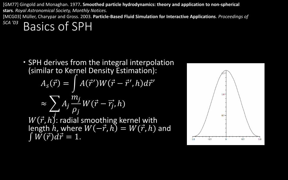
Basics of SPH

SPH derives from the integral interpolation (similar to Kernel Density Estimation):

𝐴𝑠 𝑟 = 𝐴 𝑟′ 𝑊 𝑟 − 𝑟′, ℎ 𝑑 𝑟′

≈

𝑗

𝐴𝑗𝑚𝑗

𝜌𝑗𝑊( 𝑟 − 𝑟𝑗 , ℎ)

𝑊 𝑟, ℎ : radial smoothing kernel with length ℎ, where 𝑊 − 𝑟, ℎ = 𝑊( 𝑟, ℎ) and 𝑊 𝑟 𝑑 𝑟 = 1.

[GM77] Gingold and Monaghan. 1977. Smoothed particle hydrodynamics: theory and application to non-spherical stars. Royal Astronomical Society, Monthly Notices. [MCG03] Müller, Charypar and Gross. 2003. Particle-Based Fluid Simulation for Interactive Applications. Proceedings of SCA ’03

Application to Navier-Stokes

𝜌 𝑟𝑖 =

𝑗

𝑚𝑗𝑊(𝑟𝑖 − 𝑟𝑗 , ℎ)

𝐹𝑖𝑝𝑟𝑒𝑠𝑠𝑢𝑟𝑒

= −𝛻𝑝 𝑟𝑖 = −

𝑗

𝑚𝑖𝑚𝑗𝑝𝑖

𝜌𝑖2 +𝑝𝑗

𝜌𝑗2 𝛻𝑊 𝑟𝑖 − 𝑟𝑗 , ℎ

𝑝𝑖 = 𝑘(𝜌𝑖 − 𝜌0), the ideal gas state equation [MCG03]

𝐹𝑖𝑣𝑖𝑠𝑐𝑜𝑠𝑖𝑡𝑦

= 𝜂𝛻 ⋅ 𝛻𝑢 𝑟𝑖 = 𝜂

𝑗

𝑚𝑗𝑢𝑗 − 𝑢𝑖

𝜌𝑗𝛻 ⋅ 𝛻𝑊 𝑟𝑖 − 𝑟𝑗 , ℎ

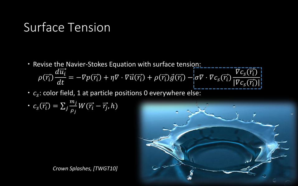
Surface Tension

Revise the Navier-Stokes Equation with surface tension:

𝜌 𝑟𝑖𝑑𝑢𝑖𝑑𝑡= −𝛻𝑝 𝑟𝑖 + 𝜂𝛻 ⋅ 𝛻𝑢 𝑟𝑖 + 𝜌 𝑟𝑖 𝑔 𝑟𝑖 − 𝜎𝛻 ⋅ 𝛻𝑐𝑠(𝑟𝑖)

𝛻𝑐𝑠(𝑟𝑖)

|𝛻𝑐𝑠(𝑟𝑖)|

𝑐𝑠: color field, 1 at particle positions 0 everywhere else:

𝑐𝑠 𝑟𝑖 = 𝑗𝑚𝑗

𝜌𝑗𝑊(𝑟𝑖 − 𝑟𝑗 , ℎ)

Crown Splashes, [TWGT10]

Kernels

The Poly6 kernel [MCG03]:

𝑊𝑝𝑜𝑙𝑦6 𝑟, ℎ =315

64𝜋ℎ9ℎ2 − 𝑟 2 3, 0 ≤ | r| ≤ h

The pressure kernel:

𝑊𝑝𝑟𝑒𝑠𝑠𝑢𝑟𝑒 𝑟, ℎ =15

𝜋ℎ6ℎ − | 𝑟| 3, 0 ≤ 𝑟 ≤ ℎ

The viscosity kernel:

𝑊𝑣𝑖𝑠𝑐𝑜𝑠𝑖𝑡𝑦 𝑟, ℎ =15

2𝜋ℎ3−| 𝑟|3

2ℎ3+| 𝑟|2

ℎ2+ℎ

2| 𝑟|− 1 , 0 ≤ 𝑟 ≤ ℎ

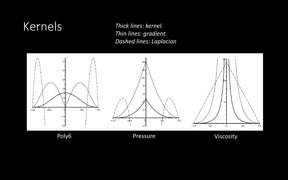
Kernels

Poly6 Pressure Viscosity

Thick lines: kernel. Thin lines: gradient.Dashed lines: Laplacian

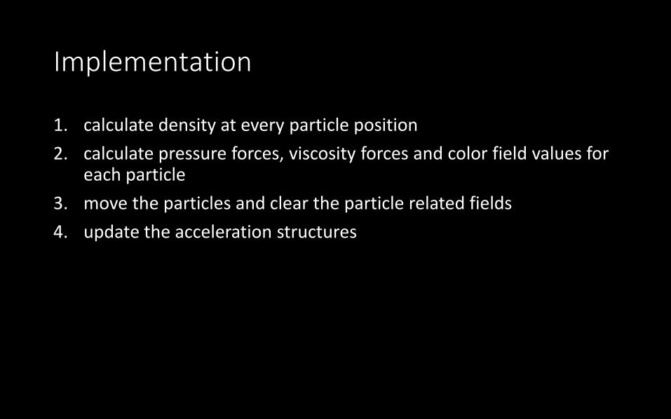
Implementation

1. calculate density at every particle position

2. calculate pressure forces, viscosity forces and color field values for each particle

3. move the particles and clear the particle related fields

4. update the acceleration structures

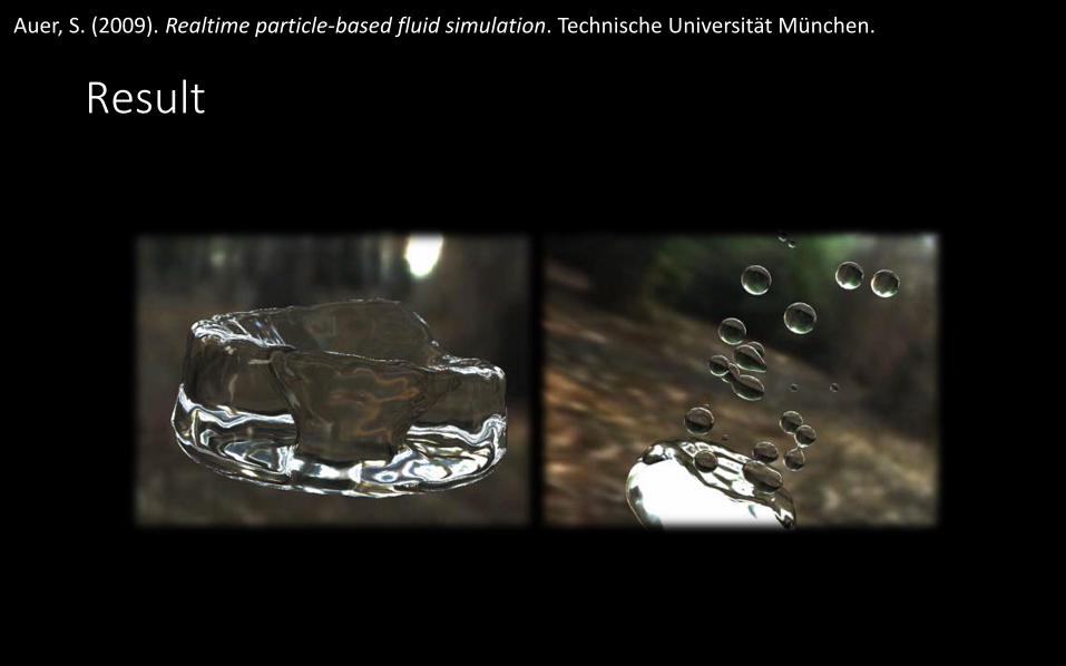
Result

Auer, S. (2009). Realtime particle-based fluid simulation. Technische Universität München.

WCSPH & PCISPHMaintain the Incompressibility

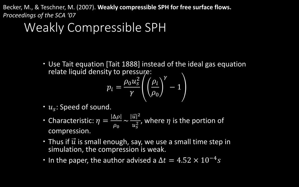
Weakly Compressible SPH

Use Tait equation [Tait 1888] instead of the ideal gas equation relate liquid density to pressure:

𝑝𝑖 =𝜌0𝑢𝑠2

𝛾

𝜌𝑖𝜌0

𝛾

− 1

𝑢𝑠: Speed of sound.

Characteristic: 𝜂 =Δ𝜌

𝜌0~𝑢 2

𝑢𝑠2 , where 𝜂 is the portion of

compression.

Thus if 𝑢 is small enough, say, we use a small time step in simulation, the compression is weak.

In the paper, the author advised a Δ𝑡 = 4.52 × 10−4𝑠

Becker, M., & Teschner, M. (2007). Weakly compressible SPH for free surface flows. Proceedings of the SCA ‘07

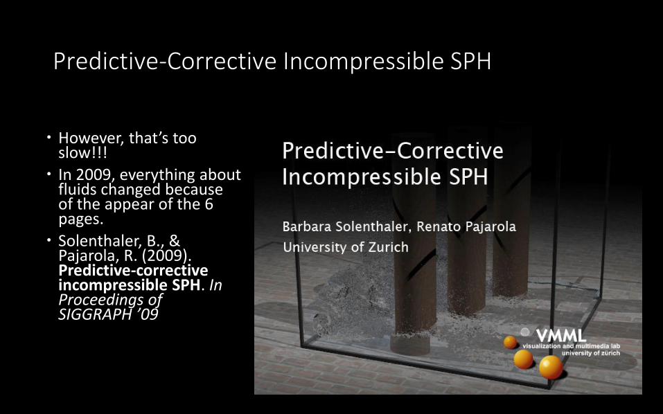
Predictive-Corrective Incompressible SPH

However, that’s too slow!!!

In 2009, everything about fluids changed because of the appear of the 6 pages.

Solenthaler, B., & Pajarola, R. (2009). Predictive-corrective incompressible SPH. In Proceedings of SIGGRAPH ’09

PCISPH—Derivation

𝜌 𝑟𝑖 , 𝑡 + 1 = 𝑗𝑚𝑗𝑊 𝑟𝑖 𝑡 + 1 − 𝑟𝑗 𝑡 + 1 , ℎ

=

𝑗

𝑚𝑗𝑊 𝑟𝑖 𝑡 + Δ𝑟𝑖 𝑡 − 𝑟𝑗 𝑡 − Δ𝑟𝑗(𝑡), ℎ

≡

𝑗

𝑚𝑗𝑊 𝑑𝑖𝑗 𝑡 + Δ𝑑𝑖𝑗 𝑡 , ℎ

where 𝑑𝑖𝑗 = 𝑟𝑖 − 𝑟𝑗.

PCISPH—Derivation

Applying Taylor approximation:

𝜌 𝑟𝑖 , 𝑡 + 1 =

𝑗

𝑚𝑗𝑊 𝑑𝑖𝑗 𝑡 + Δ𝑑𝑖𝑗 𝑡 , ℎ

=

𝑗

𝑚𝑗 𝑊 𝑑𝑖𝑗 𝑡 , ℎ + 𝛻𝑊 𝑑𝑖𝑗 𝑡 , ℎ ⋅ Δ𝑑𝑖𝑗 𝑡

= 𝜌𝑖 𝑡 + Δ𝜌𝑖 𝑡

∴ Δ𝜌𝑖 𝑡 =

𝑗

𝑚𝑗𝛻𝑊𝑖𝑗 ⋅ Δ𝑟𝑖 𝑡 − Δ𝑟𝑗 𝑡

= Δ𝑟𝑖 𝑡

𝑗

𝑚𝑗𝛻𝑊𝑖𝑗 −

𝑗

mj𝛻𝑊𝑖𝑗Δ𝑟𝑗 𝑡 (∗)

PCISPH—Derivation

Neglecting all forces but the pressure (from 𝐹 = 𝑚𝑎):

Δ𝑟𝑖 = Δ𝑡2𝐹𝑖𝑝𝑟𝑒𝑠𝑠𝑢𝑟𝑒

𝑚𝑖assuming that neighbors have equal pressures 𝑝𝑖

′ and all densities are equal to the rest density 𝜌0 (according to the incompressibility condition):

𝐹𝑖𝑝𝑟𝑒𝑠𝑠𝑢𝑟𝑒

= −

𝑗

𝑚𝑖𝑚𝑗𝑝𝑖′

𝜌02 +𝑝𝑖′

𝜌02 𝛻𝑊𝑖𝑗 = −𝑚𝑖

2𝑝𝑖′

𝜌02

𝑗

mj𝛻𝑊𝑖𝑗

Inserting back, we have:

Δ𝑟𝑖 = −Δ𝑡22𝑝𝑖′

𝜌02

𝑗

mj𝛻𝑊𝑖𝑗

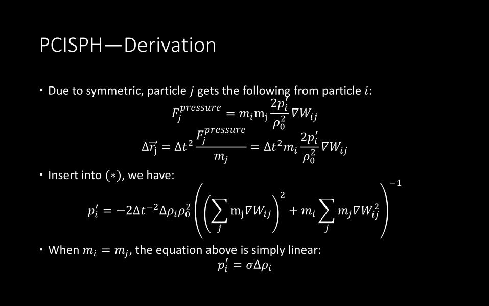
PCISPH—Derivation

Due to symmetric, particle 𝑗 gets the following from particle 𝑖:

𝐹𝑗𝑝𝑟𝑒𝑠𝑠𝑢𝑟𝑒

= 𝑚𝑖mj2𝑝𝑖′

𝜌02 𝛻𝑊𝑖𝑗

Δ𝑟j = Δ𝑡2𝐹𝑗𝑝𝑟𝑒𝑠𝑠𝑢𝑟𝑒

𝑚𝑗= Δ𝑡2𝑚𝑖

2𝑝𝑖′

𝜌02 𝛻𝑊𝑖𝑗

Insert into (∗), we have:

𝑝𝑖′ = −2Δ𝑡−2Δ𝜌𝑖𝜌0

2

𝑗

mj𝛻𝑊𝑖𝑗

2

+𝑚𝑖

𝑗

𝑚𝑗𝛻𝑊𝑖𝑗2

−1

When 𝑚𝑖 = 𝑚𝑗, the equation above is simply linear:𝑝𝑖′ = 𝜎Δ𝜌𝑖

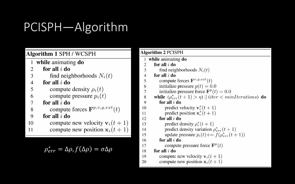
PCISPH—Algorithm

𝜌𝑒𝑟𝑟∗ = Δ𝜌, 𝑓 Δ𝜌 = 𝜎Δ𝜌

Adaptive Time-steppingBe robust

Ihmsen, M., & Gissler, M. (2010). Boundary handling and adaptive time-stepping for PCISPH. In Proceedings of VRIPHYS ‘10

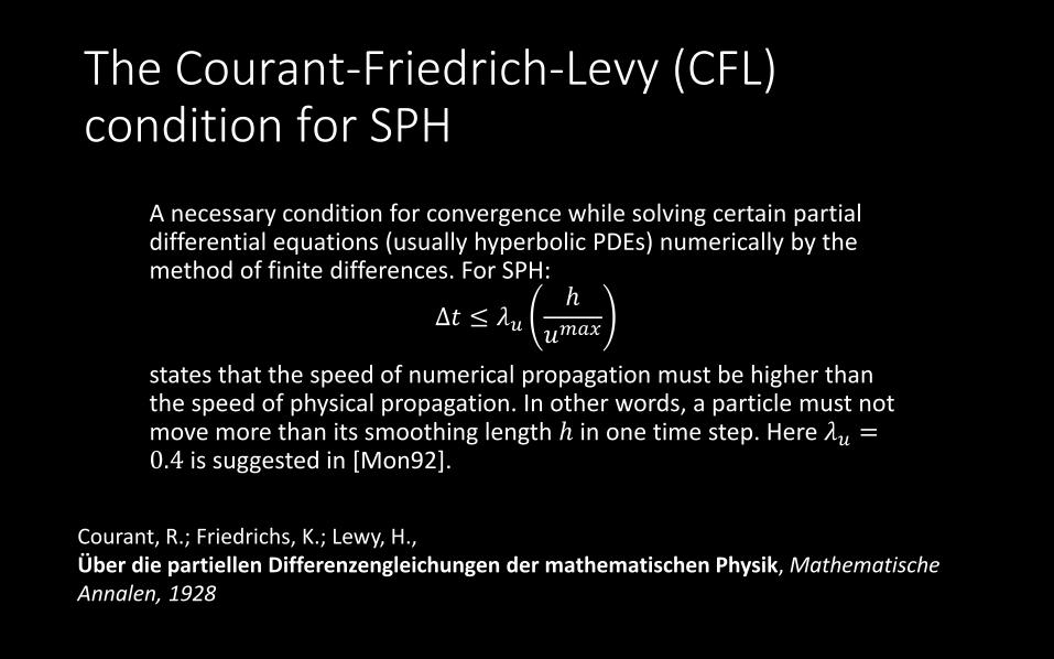
The Courant-Friedrich-Levy (CFL) condition for SPH

A necessary condition for convergence while solving certain partial differential equations (usually hyperbolic PDEs) numerically by the method of finite differences. For SPH:

Δ𝑡 ≤ 𝜆𝑢ℎ

𝑢𝑚𝑎𝑥

states that the speed of numerical propagation must be higher than the speed of physical propagation. In other words, a particle must not move more than its smoothing length ℎ in one time step. Here 𝜆𝑢 =0.4 is suggested in [Mon92].

Courant, R.; Friedrichs, K.; Lewy, H., Ü ber die partiellen Differenzengleichungen der mathematischen Physik, Mathematische Annalen, 1928

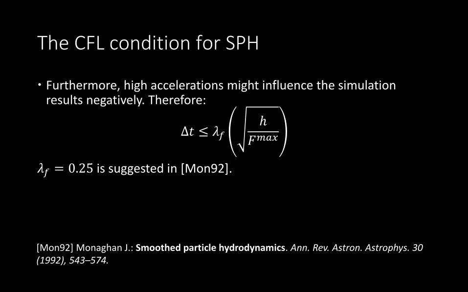
The CFL condition for SPH

Furthermore, high accelerations might influence the simulation results negatively. Therefore:

Δ𝑡 ≤ 𝜆𝑓ℎ

𝐹𝑚𝑎𝑥

𝜆𝑓 = 0.25 is suggested in [Mon92].

[Mon92] Monaghan J.: Smoothed particle hydrodynamics. Ann. Rev. Astron. Astrophys. 30 (1992), 543–574.

The Strategy

Initial time step: Δ𝑡 = 0.25ℎ

𝑢0𝑚𝑎𝑥 . During the simulation, the time

step is:

Increased 0.2% if: Decreased 0.2% if:

0.19ℎ

𝐹𝑡𝑚𝑎𝑥 > Δ𝑡

Δ𝜌𝑚𝑎𝑥 < 4.5𝜂𝑎𝑣𝑔Δ𝜌𝑎𝑣𝑔 < 0.9𝜂𝑎𝑣𝑔

0.39ℎ

𝑢𝑡𝑚𝑎𝑥 > Δ𝑡

0.2ℎ

𝐹𝑡𝑚𝑎𝑥 < Δ𝑡

Δ𝜌𝑚𝑎𝑥 > 5.5𝜂𝑎𝑣𝑔Δ𝜌𝑎𝑣𝑔 > 𝜂𝑎𝑣𝑔

0.4ℎ

𝑢𝑡𝑚𝑎𝑥 ≤ Δ𝑡

Ghost SPHFix the Boundary Condition

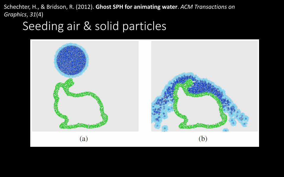
Seeding air & solid particles

Schechter, H., & Bridson, R. (2012). Ghost SPH for animating water. ACM Transactions on Graphics, 31(4)

Seeding air & solid particles

Solve the particle deficiency at boundaries and eliminate artifacts by:

1. dynamically seeding ghost particles in a layer of air around the liquid with a blue noise distribution.

2. Extrapolating the right quantities from the liquid to the air and solid ghost particles to enforce the correct boundary conditions.

3. using the ghost particles appropriately in summations.

Ghost Particles in the Air

𝑚𝑎𝑖𝑟 = 𝑚𝑙𝑖𝑞𝑢𝑖𝑑𝑢𝑎𝑖𝑟 = 𝑛𝑒𝑎𝑟𝑒𝑠𝑡 𝑢𝑙𝑖𝑞𝑢𝑖𝑑𝜌𝑎𝑖𝑟 = 𝜌0

thus 𝑝𝑎𝑖𝑟 = 0.

Resample every 10 time steps (twice per frame)

Ghost Particles in the Solid

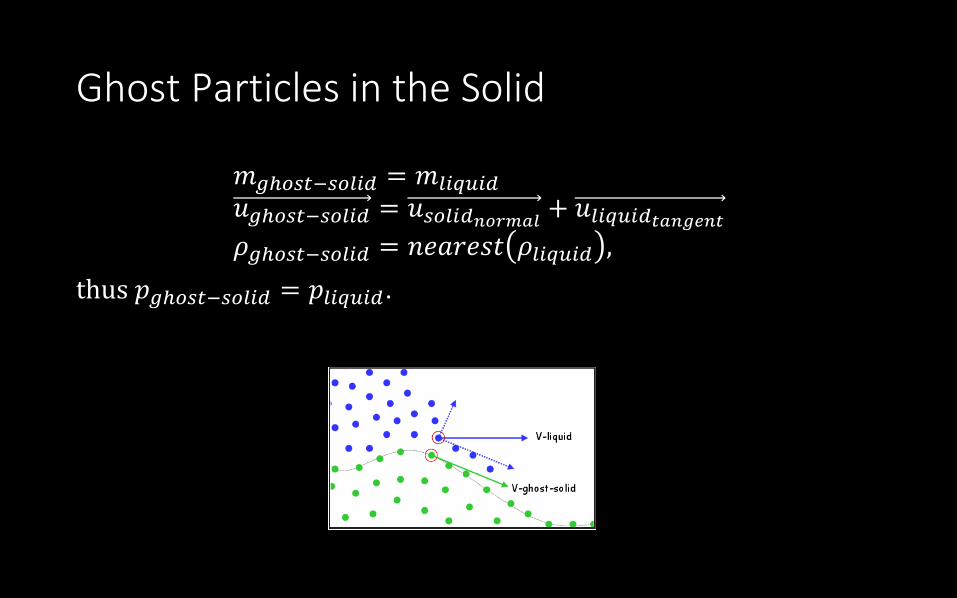
𝑚𝑔ℎ𝑜𝑠𝑡−𝑠𝑜𝑙𝑖𝑑 = 𝑚𝑙𝑖𝑞𝑢𝑖𝑑𝑢𝑔ℎ𝑜𝑠𝑡−𝑠𝑜𝑙𝑖𝑑 = 𝑢𝑠𝑜𝑙𝑖𝑑𝑛𝑜𝑟𝑚𝑎𝑙 + 𝑢𝑙𝑖𝑞𝑢𝑖𝑑𝑡𝑎𝑛𝑔𝑒𝑛𝑡𝜌𝑔ℎ𝑜𝑠𝑡−𝑠𝑜𝑙𝑖𝑑 = 𝑛𝑒𝑎𝑟𝑒𝑠𝑡 𝜌𝑙𝑖𝑞𝑢𝑖𝑑 ,

thus 𝑝𝑔ℎ𝑜𝑠𝑡−𝑠𝑜𝑙𝑖𝑑 = 𝑝𝑙𝑖𝑞𝑢𝑖𝑑.

Ghost Sampling

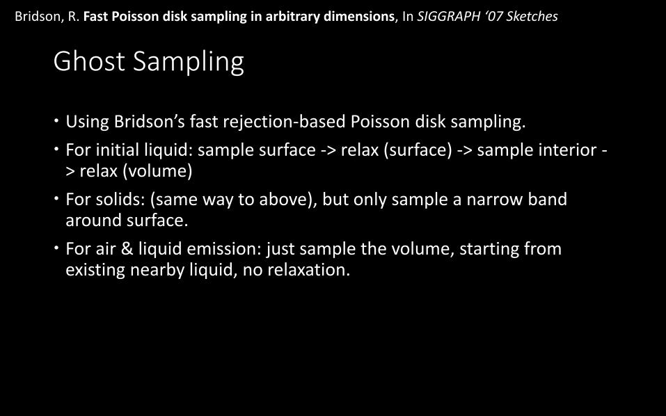
Using Bridson’s fast rejection-based Poisson disk sampling.

For initial liquid: sample surface -> relax (surface) -> sample interior -> relax (volume)

For solids: (same way to above), but only sample a narrow band around surface.

For air & liquid emission: just sample the volume, starting from existing nearby liquid, no relaxation.

Bridson, R. Fast Poisson disk sampling in arbitrary dimensions, In SIGGRAPH ‘07 Sketches

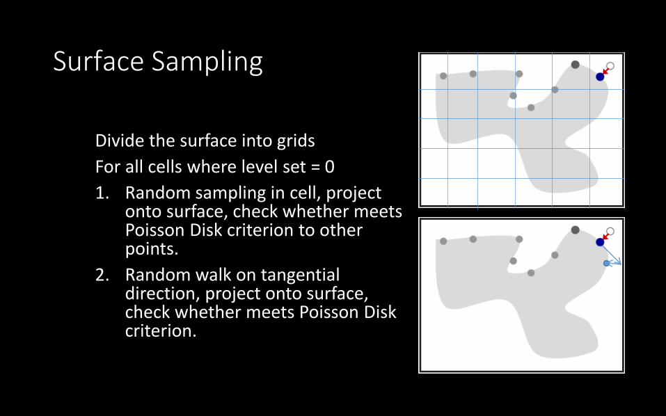
Surface Sampling

Divide the surface into grids

For all cells where level set = 0

1. Random sampling in cell, project onto surface, check whether meets Poisson Disk criterion to other points.

2. Random walk on tangential direction, project onto surface, check whether meets Poisson Disk criterion.

Interior Sampling

1. Initialize a random sample and a list of sample indices (active list).

2. While the active list is not empty, choose a random sample from it (say 𝑥𝑖).

3. Generate up to k points chosen uniformly from the spherical annulus between radius r and 2r around 𝑥𝑖. For each point in turn, check if it is within distance r of existing samples.

4. If a point is adequately far from existing samples, emit it as the next sample and add it to the active list. Return to 2.

Spatial AdaptabilityLess particles, faster simulation

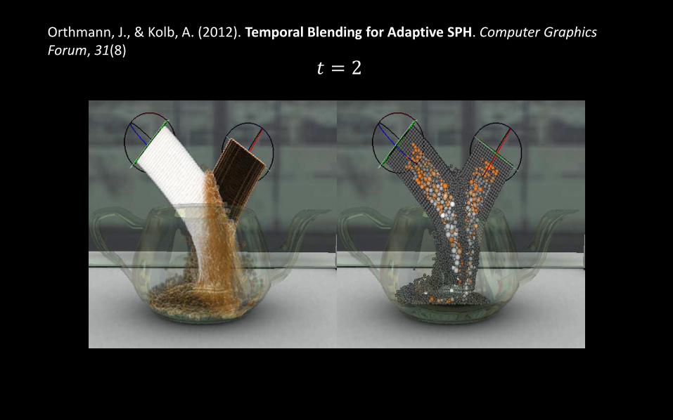
𝑡 = 2

Orthmann, J., & Kolb, A. (2012). Temporal Blending for Adaptive SPH. Computer Graphics Forum, 31(8)

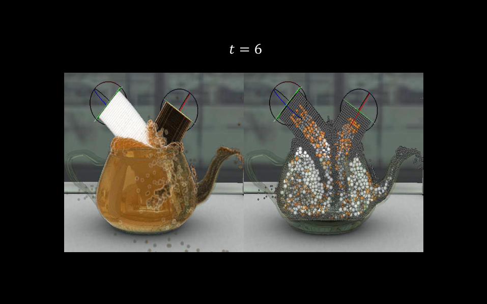
𝑡 = 6

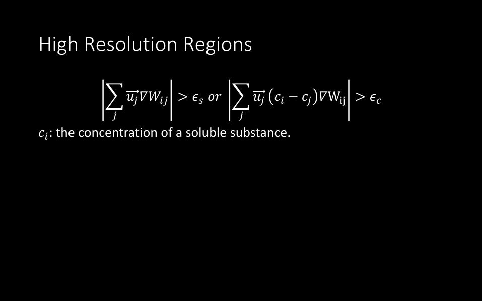
High Resolution Regions

𝑗

𝑢𝑗𝛻𝑊𝑖𝑗 > 𝜖𝑠 𝑜𝑟

𝑗

𝑢𝑗 𝑐𝑖 − 𝑐𝑗 𝛻Wij > 𝜖𝑐

𝑐𝑖: the concentration of a soluble substance.

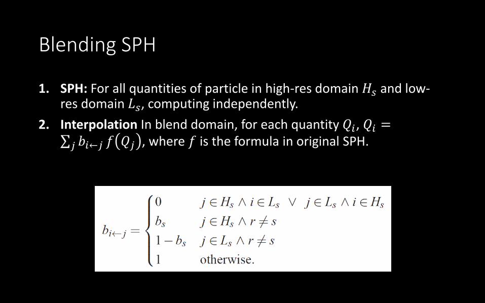
Blending SPH

1. SPH: For all quantities of particle in high-res domain 𝐻𝑠 and low-res domain 𝐿𝑠, computing independently.

2. Interpolation In blend domain, for each quantity 𝑄𝑖, 𝑄𝑖 = 𝑗 𝑏𝑖←𝑗 𝑓 𝑄𝑗 , where 𝑓 is the formula in original SPH.

Blending SPH

3. Interpolation quantities between domains:

Z—indexing Hardware Acceleration

Parallelizing SPH on the GPUComputing for each particle is simple. However, the most difficult part for parallelization is the neighbor searching.

Goswami, P., & Schlegel, P. (2010). Interactive SPH simulation and rendering on the GPU. Proceedings of the SCA ‘10

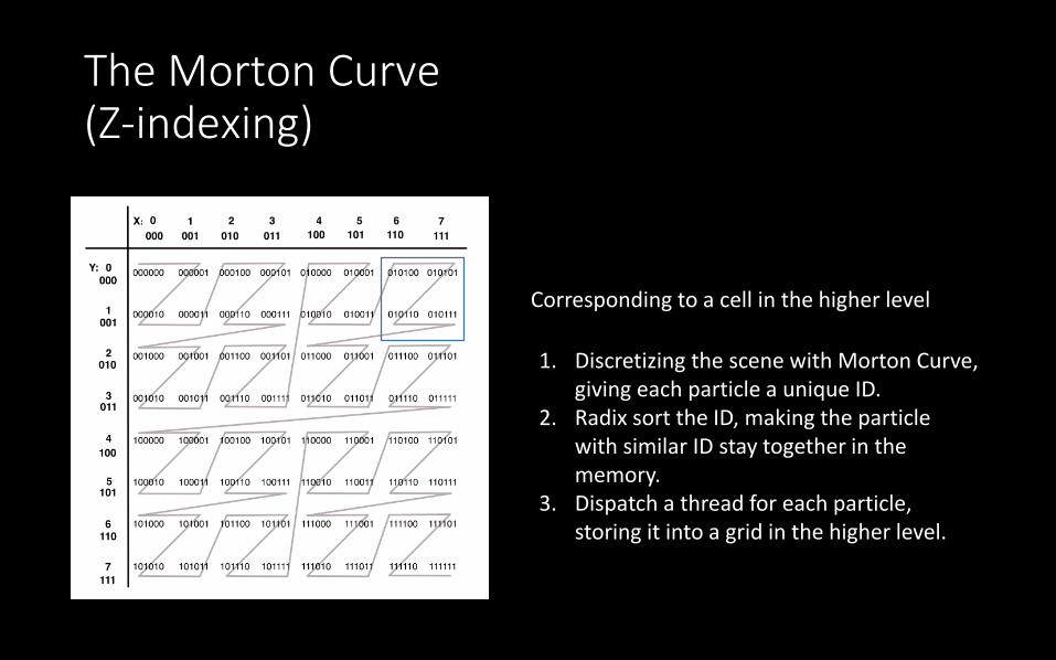
The Morton Curve (Z-indexing)

Corresponding to a cell in the higher level

1. Discretizing the scene with Morton Curve, giving each particle a unique ID.

2. Radix sort the ID, making the particle with similar ID stay together in the memory.

3. Dispatch a thread for each particle, storing it into a grid in the higher level.

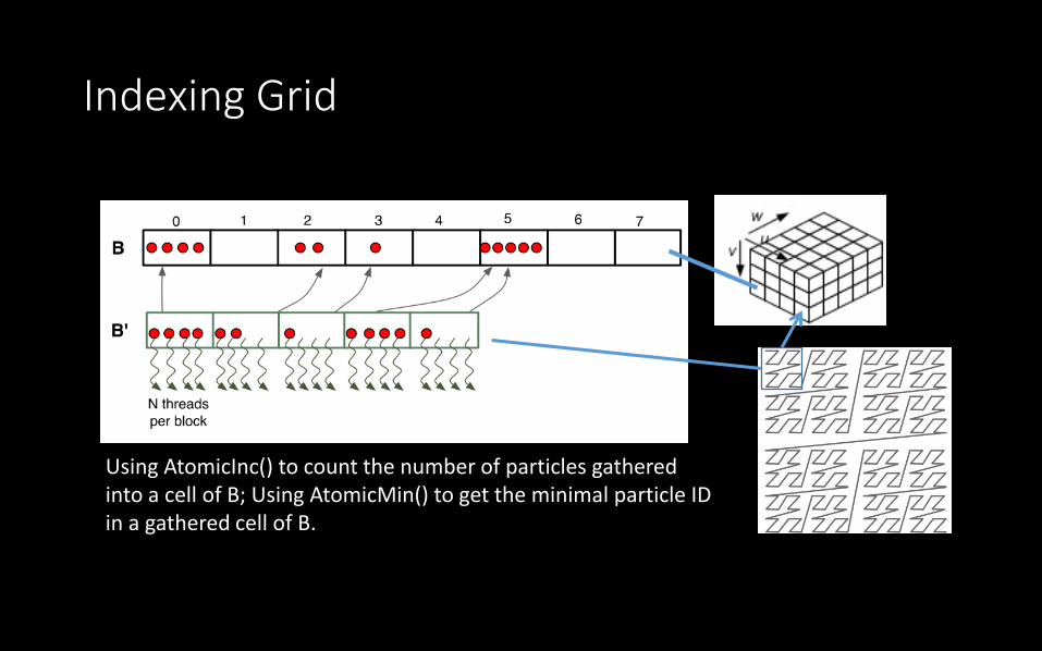
Indexing Grid

Using AtomicInc() to count the number of particles gathered into a cell of B; Using AtomicMin() to get the minimal particle ID in a gathered cell of B.

Implicit Surface TrackingFrom Points to Surface

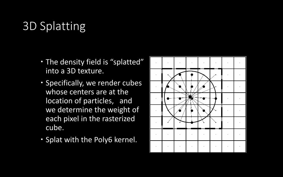
3D Splatting

The density field is “splatted” into a 3D texture.

Specifically, we render cubes whose centers are at the location of particles, and we determine the weight of each pixel in the rasterized cube.

Splat with the Poly6 kernel.

3D Splatting

3D Splatting

Slices of the 3D density texture.

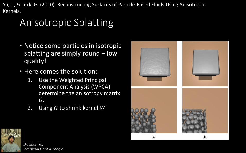
Anisotropic Splatting

Notice some particles in isotropic splatting are simply round – low quality!

Here comes the solution:1. Use the Weighted Principal

Component Analysis (WPCA) determine the anisotropy matrix 𝐺.

2. Using 𝐺 to shrink kernel 𝑊

Yu, J., & Turk, G. (2010). Reconstructing Surfaces of Particle-Based Fluids Using Anisotropic Kernels.

Dr. Jihun Yu, Industrial Light & Magic

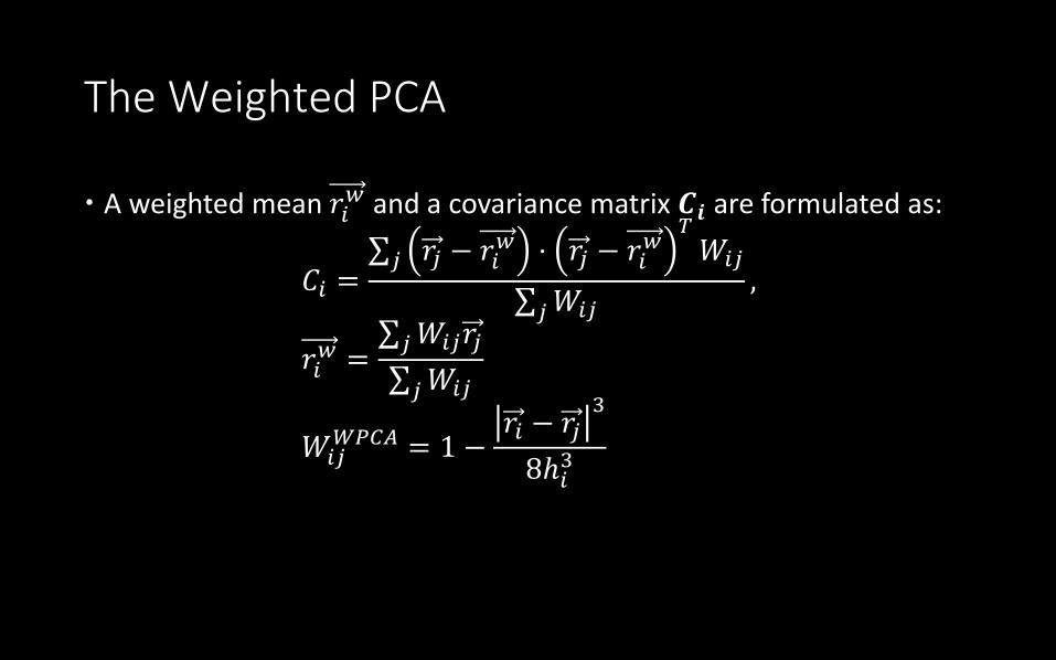
The Weighted PCA

A weighted mean 𝑟𝑖𝑤 and a covariance matrix 𝑪𝒊 are formulated as:

𝐶𝑖 = 𝑗 𝑟𝑗 − 𝑟𝑖

𝑤 ⋅ 𝑟𝑗 − 𝑟𝑖𝑤𝑇𝑊𝑖𝑗

𝑗𝑊𝑖𝑗,

𝑟𝑖𝑤 = 𝑗𝑊𝑖𝑗𝑟𝑗

𝑗𝑊𝑖𝑗

𝑊𝑖𝑗𝑊𝑃𝐶𝐴 = 1 −

𝑟𝑖 − 𝑟𝑗3

8ℎ𝑖3

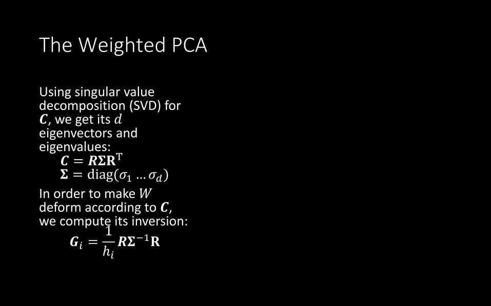
The Weighted PCA

Using singular value decomposition (SVD) for 𝑪, we get its 𝑑eigenvectors and eigenvalues:𝑪 = 𝑹𝚺𝐑T

𝚺 = diag(𝜎1…𝜎𝑑)

In order to make 𝑊deform according to 𝑪, we compute its inversion:

𝑮𝑖 =1

ℎ𝑖𝑹𝚺−1𝐑

The Marching Cubes

The Marching Cubes

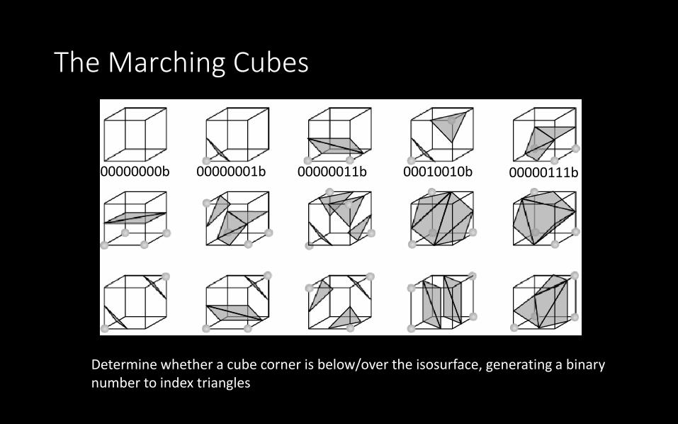
00000000b 00000001b 00000011b 00010010b 00000111b

Determine whether a cube corner is below/over the isosurface, generating a binary number to index triangles

Histopyramid (HP)

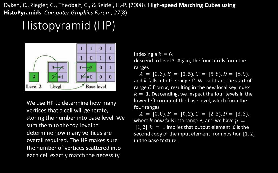
Dyken, C., Ziegler, G., Theobalt, C., & Seidel, H.-P. (2008). High-speed Marching Cubes using HistoPyramids. Computer Graphics Forum, 27(8)

Indexing a 𝑘 = 6:descend to level 2. Again, the four texels form the ranges𝐴 = [0, 3), 𝐵 = [3, 5), 𝐶 = [5, 8), 𝐷 = [8, 9),

and 𝑘 falls into the range 𝐶. We subtract the start of range 𝐶 from 𝑘, resulting in the new local key index 𝑘 = 1. Descending, we inspect the four texels in the lower left corner of the base level, which form the four ranges𝐴 = [0, 0), 𝐵 = [0, 2), 𝐶 = [2, 3), 𝐷 = [3, 3),

where 𝑘 now falls into range B, and we have 𝑝 =[1, 2]. 𝑘 = 1 implies that output element 6 is the second copy of the input element from position [1, 2] in the base texture.

We use HP to determine how manyvertices that a cell will generate, storing the number into base level. We sum them to the top level to determine how many vertices are overall required. The HP makes sure the number of vertices scattered into each cell exactly match the necessity.

Realistic Appearance – Snell’s Law and Fresnel Term

For un-polarized light, the reflection coefficient:

𝑅 = 0.5 𝑅𝑠 + 𝑅𝑝

𝑅𝑠 =sin2 𝜃𝑖 − 𝜃𝑡sin2 𝜃𝑖 + 𝜃𝑡

𝑅𝑝 =tan2 𝜃𝑖 − 𝜃𝑡tan2 𝜃𝑖 + 𝜃𝑡

Schlick’s Approximation [Sch93]:𝑅≈ 𝑅 0 + 1 − 𝑅 0 1 − cos 𝜃𝑖

5

The Snell’s Law: sin 𝜃𝑖

sin 𝜃𝑗=𝑛𝑗

𝑛𝑖

Explicit Surface TrackingComputational Geometry in Fluids

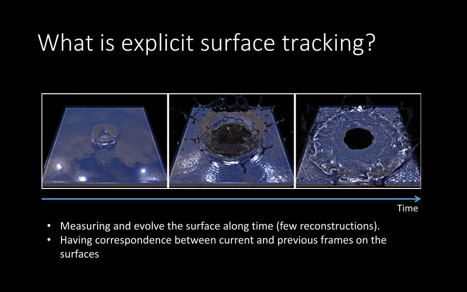
What is explicit surface tracking?

Time

• Measuring and evolve the surface along time (few reconstructions).• Having correspondence between current and previous frames on the

surfaces

Why explicit surface tracking?

Detail is perfectly preserved.

Topology changes are controlled.

Color and textures on the surface is temporal coherent.

Easy to compute PDEs on the surface, adding capillary waves and simulating surface tension.

Wojtan, C., Thürey, N., Gross, M., & Turk, G. (2009). Deforming meshes that split and merge. ACM Transactions on Graphics, 28(3), SIGGRAPH ‘09

Overview

1. Advect the mesh vertices according to SPH particle velocities

𝑥𝑛+1 = 𝑥𝑛 + 𝑗𝑊𝑖𝑗𝑢𝑗

𝑗𝑊𝑖𝑗Δ𝑡

2. Improve triangle shapes using edge split & collapse operations

3. Project mesh vertices onto the implicit surface

4. Handling topological changes

Yu, J., Wojtan, C., Turk, G., & Yap, C. (2012). Explicit Mesh Surfaces for Particle Based Fluids. Computer Graphics Forum, 31(2pt4), Eurographics 2012, 815–824.

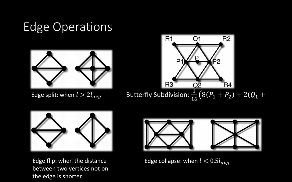
Edge Operations

Edge split: when 𝑙 > 2𝑙𝑎𝑣𝑔

Edge flip: when the distance between two vertices not on the edge is shorter

Butterfly Subdivision: 1

16 8 𝑃1 + 𝑃2 + 2(𝑄1 +

Edge collapse: when 𝑙 < 0.5𝑙𝑎𝑣𝑔

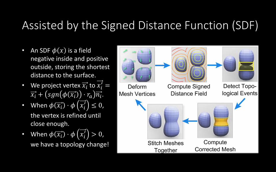
Assisted by the Signed Distance Function (SDF)

• An SDF 𝜙 𝑥 is a field negative inside and positive outside, storing the shortest distance to the surface.

• We project vertex 𝑥𝑖 to 𝑥𝑖′ =

𝑥𝑖 + 𝑠𝑔𝑛 𝜙 𝑥𝑖 ⋅ 𝑟𝑎 𝑛𝑖.

• When 𝜙 𝑥𝑖 ⋅ 𝜙 𝑥𝑖′ ≤ 0,

the vertex is refined until close enough.

• When 𝜙 𝑥𝑖 ⋅ 𝜙 𝑥𝑖′ > 0,

we have a topology change!

Deep Cell Tests

• A complex edge is an edge that intersects surface more than once.• A complex face is a square face that intersects surface in a closed loop or touches a

complex edge.• A complex cell is a cell that has any complex edges or complex faces, or any cell that

has the same sign at all of its corners while also having surface embedded inside.• A deep cell is a complex cell that is at least one cell away from the surface.• Flood fill the deep cell until a simple cell is touched

Complex cellsSDF, yellow inside Deep cells Deep cells Flood fill

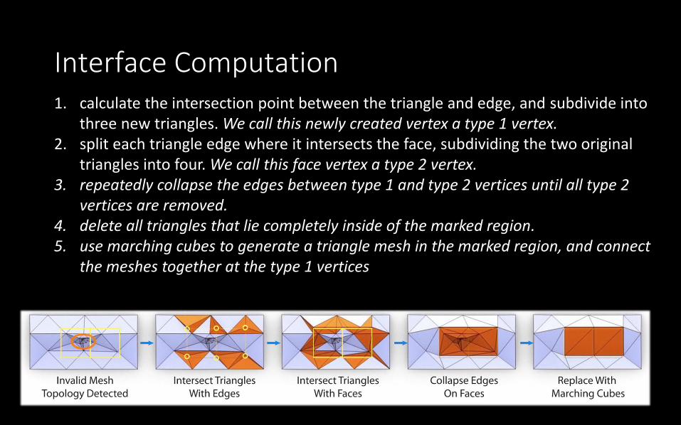
Interface Computation1. calculate the intersection point between the triangle and edge, and subdivide into

three new triangles. We call this newly created vertex a type 1 vertex.2. split each triangle edge where it intersects the face, subdividing the two original

triangles into four. We call this face vertex a type 2 vertex.3. repeatedly collapse the edges between type 1 and type 2 vertices until all type 2

vertices are removed.4. delete all triangles that lie completely inside of the marked region.5. use marching cubes to generate a triangle mesh in the marked region, and connect

the meshes together at the type 1 vertices

Other topics

1. Fluid-fluid coupling

2. Fluid-solid coupling

3. Compressible flow &Turbulence

4. Large-scale simulation

5. 2D SPH & 2.5D SPH

6. Mesh registration &tracking & evolving

7. GPU acceleration for mesh-based tracking

8. Handling detailed surface

9. Polyhedral (irregular) fluidsimulation