The inuence of light/dark adaptation and lateral ... · The inuence of light/dark adaptation and...

The influence of light/dark adaptation and lateral inhibition onphototaxic foraging.

A hypothetical-animal study

(7th March 2002)

Adaptive Behavior, Vol. 5, No. 2: 141 - 167

�. � . � . � ertin �� ([email protected])

. . van de � rind � ([email protected])

1: Current address:LPPA

College de France / C.N.R.S.11, place Marcelin Berthelot

75005 ParisFrance

fax: +33 1 442713822: Neuroethology group

Department of Comparative PhysiologyUtrecht University

&

Padualaan 83584 CH Utrechtthe Netherlands

fax: +31 30 2542219/2532837

2

The influence of light/dark adaptation and lateral inhibition on phototaxic foraging.

Abstract

Vision did not arise and evolve to just ”see” things, but rather to act on and interact with the habitat.Thus it might be misleading to study vision without its natural coupling to vital action. Here we invest-igate this problem in a simulation study of the simplest kind of visually-guided foraging by a speciesof 2D hypothetical animal called the (diurnal) paddler. In a previous study, we developed a hypothet-ical animal called the archaepaddler, which used positive phototaxis to forage for autoluminescent preyin a totally dark environment (the deep-sea). Here we discuss possible visual mechanisms that allow(diurnal) paddlers to live in shallower water, foraging for light-reflecting prey in ambient light. Themodification consists of two stages. In the first stage Weber adaptation compresses the retinal illumin-ation into an acceptable range of neural firing frequencies. In the second stage highpass filtering withlateral inhibition separates background responses from foreground responses. We report on a number ofparameter-studies conducted with the foraging diurnal paddler, in which the influence of dark/light ad-aptation and lateral inhibition on foreground/background segregation and foraging performance (”fit-ness”) are quantified. It is shown that the paddler can survive adequately for a substantial range ofparameters that compromises between discarding as much unwanted visual (background) informationas possible, whilst retaining as much information on potential prey as possible. Parameter values thatoptimise purely visual performance like foreground/background segregation are not always optimalfor foraging performance and vice versa. This shows that studies of vision might indeed require moreserious consideration of the goals of vision and the ethogram of the studied organisms than has beencustomary.

Keywords: dark/light adaptation, lateral inhibition, hypothetical animal, phototaxic navigation,Weber adaptation.

c�

1997,2002 R.J.V. Bertin

1 INTRODUCTION 3

1 Introduction

Vision is usually studied without direct recourse to suitable actions of the studied organism. Since thecoupling of animals to their habitat concerns a loop of processes of the type ”sensory interpretative motor habitat sensory ...”, purely visual studies might give a rather limited and biased viewof visually-guided organism/habitat interactions (Gibson 1979; van de Grind 1990). In principle, electro-physiological studies of behaving animals provide one possibility to improve this situation. However,this approach is virtually impossible in the case of soft-bodied or small animals. Unfortunately it is inthese animals that visually-guided behaviour should be studied in the first place to get some insight inits evolutionary beginnings and early development. Even in larger animals there is hardly a possibilityto use ”in-eco” electrophysiology for other than rather simple (non-vital) actions, such as making an eye-saccade or pushing a button. One alternative is offered by the present hypothetical-animal approach. Insuch a computer-simulation study one develops a hypothetical animal performing some natural actionand then studies the influence of all processes involved in the continuous perception-action loop, whileit is in place and complete. Of course, the initial approaches are bound to be a bit clumsy. One first needsan acceptable ”platform”, performing the simulated action with sufficient dexterity. The action has to benatural and it has to be simulated in a physically and biologically realistic way and in sufficient detail.Once a certain quality of the platform is reached one can ”play” with all the interactions and — in thecontext of studies of vision — study the contribution of all sorts of visual mechanisms to the behaviourunder study.

This general idea motivated us to embark on an extensive study of hypothetical animals that performnatural actions in a biologically plausible way, and in which the animal/habitat interactions are physicallyrealistic. Our hypothetical animals do not mimic specific real animals; we aim for a realistic embodimentof specific perception-action loops. The success of this approach depends on the biological realism ofeach of the aspects of the perception-action loop and is not measured by the question whether or notthe results reproduce the behaviour of a specific living animal. After all there are many missing links inthe evolution of, say, navigation behaviour, but that does not preclude the development of reasonabletheories as long as the known (physical and biological) boundary conditions are meticulously taken intoconsideration.

We have recently designed and simulated a species of hypothetical deep sea animal, called archae-paddler, that hunts autoluminescent prey, called glowballs, in an otherwise dark surround (Bertin & vande Grind 1996). Since the animal lives in the water-layer just above the bottom of the deep sea, we largelyignore the third dimension, essentially modelling the animal in 2D. Its foraging behaviour is phototaxic � ,and the rather primitive eyes drive the contralateral paddles.

There are several levels of detail in which acting animals can be modelled. In general, more complexbehaviours are best modelled at a higher, more schematic level of description (e.g. Corbacho & Arbib,1995), with less relevant, lower-level biophysical aspects approximated or taken for granted (e.g. thephysics of locomotion; the animal might be able to move two steps forward and one to the side). However,since the animal’s actions are its interactions with its environment, they directly influence its sensoryinput. Therefore studies in which sensorimotor behaviour is modelled at a lower level of description (e.g.Cliff, Husbands & Harvey 1993, Ekeberg, Lansner & Grillner 1995 or Cruse et al. 1995), and also studiesaiming at realistic animation of behaviour (e.g. Terzopoulos, Tu & Grzeszczuk 1994) do explicitly modelthese physical aspects.

In our model, we simulate the physical processes of locomotion in sufficient detail, making the pad-dling realistic enough to view it as an adequate model of real-animal paddling (Bertin & van de Grind1996). Since the anatomical and physical parameters proved to allow ample variation before the for-aging quality began to break down, the simulated animal can be viewed as occupying a stable region of”design” space (in the sense of Dennett, 1995), allowing quite some genotypic variation. It is interestingto note that the geometry of such an animal depends on habitat-factors, such as prey-density and spa-tial prey distribution and on the simulated behavioural foraging strategy. Changes of the habitat and/or�

Kuhn (1919), following Loeb (1918) defined tropotaxis as a kind of autonomous closed- loop navigation in which sensory excita-tion in the nervous system is kept (left-right) symmetric by motor actions governed by the same sensory information. This principleis nicely illustrated in Braitenberg (1984), but also in Walter (1950, 1951). Tropotaxis of chemical nature is demonstrated in Beer(1990).

1 INTRODUCTION 4

behavioural strategy are immediately reflected in the body-geometry as required for optimal perform-ance (Bertin and van de Grind 1996). Here we take the ”average paddler” and ”average habitat” of theprevious study as our starting point and study the influence of increasing visual sophistication on thephototaxic foraging success. The foraging strategy, as embodied in the animal’s nervous system, is thesame as in the previous study: move in the direction of the strongest light response. This response is notan unprocessed reflection of the light distribution, since that would entail continuous course changes.Rather, the eyes have simple (Gaussian) tuning characteristics for direction, and binocular facilitationgives a slight bias for coursing straight ahead if there is prey in that direction. The visual information isthus preprocessed such that a balance is struck between on the one hand as large a field of view as pos-sible (maximisation of information), and on the other hand the possibility to ”selectively concentrate” ononly a small part of the visual field. This compromise depends of course on the animal’s habitat (Bertin& van de Grind 1996; see also Cliff & Bullock 1993 for a slightly different approach).

The resulting navigation is a rather uncomplicated kind of visual navigation, which we call ”photo-taxic foraging”. Light is food and the strongest light is the most or the nearest food.

The archaepaddlers of the previous study lived in a dark environment and any light blob was re-garded as food (a glowball). Thus there was no problem of segregating object and background, nor wasthere any need for contrast enhancement or separate ON or OFF channels � . In this paper we study thecase of an evolving group of paddlers moving towards shallower water, where background light starts tointerfere with the detection of autoluminescent prey. In the new habitat, different prey is available thatreflects more light than it produces. Even nonreflecting edible objects, e.g. silhouetted against the brightsurface right above our hunting paddlers, might become a meal if the paddler’s visual system could de-velop dark-object detecting capabilities. One need not simulate the evolution process itself in this case,since it is known that the standard response of evolving visual systems to these challenges is to developON and OFF (and/or ON/OFF) cells and lateral inhibition to aid foreground/background segregation. Onecan view the Limulus visual system as a paradigm in this respect (Hartline & Ratliff 1974).

It is rather obvious, however, that this is not sufficient. One also needs to introduce circuitry to allowlight and dark adaptation, so that the ON and OFF units can function satisfactorily over a wide range ofbackground luminances, without the risk of saturation at higher luminance levels, and loss of preciousinformation at low levels. We therefore implemented one of the simplest and most ubiquitous adapta-tion principles: Weber-law adaptation (see e.g. Bouman, van de Grind and Zuidema 1985, or Shapleyand Enroth-Cugell 1984). An interesting property of this type of adaptation is that it emphasizes reflect-ancy (Shapley and Enroth-Cugell 1984). Nothing in the principles on which the resulting visual systemis based is surprising or new, yet it is certainly not a priori clear that the new species of paddler equippedwith this extremely simple diurnal visual system can successfully forage in shallow water at a varietyof background light levels. In particular it is not a priori clear whether (and how much) lateral inhibi-tion or light/dark adaptation contribute to foraging success. To study this question we first develop aquality-measure for the foraging behaviour (which requires side-stepping the notorious travelling sales-man problem) and then study the influence of various parameters of the visual system on this quality-measure. Also the performance of the previous archaepaddler can serve as a performance-reference, tobe called the ”dark reference”. This is based on the fact that in a simulation, one can transform the en-vironment of a (diurnal) paddler into a deep-sea habitat by setting the background level at zero. Thenthe deep-sea paddler (archaepaddler or dark reference) can hunt in the transformed environment andits performance can serve as an adaptation-free and inhibition-free reference value. The importance ofadaptation and inhibition can thus be appreciated by comparing the performance of a diurnal paddlerwith the performance of an archaepaddler in the same environment.

To keep the exposition sufficiently simple we de-emphasize the detection of objects darker than thebackground and concentrate on the detection of objects brighter than the background. The simulationallows us to quantify the merits for hunting success of lateral inhibition and of the automatic gain con-trol of Weber’s law. Pitting these different aspects of vision against each other is only possible in thisparticular kind of approach, with an explicit and biologically reasonable measure of success for the en-suing visually-guided behaviour. This opens exciting perspectives for testing theories of vision, and inanother paper we will test a theory of motion vision. Here the main question is: What is the relative meritof lateral inhibition (of a simple Limulus type) and of Weber adaptation, alone or in combination, for�

Sets of neur(on)al connections that respond to increases or decreases in (visual) input.

2 THE DIURNAL PADDLER 5

simple visually-guided hunting (phototaxic navigation) in a shallow aquatic environment with variablebackground light levels?

2 The diurnal paddler

This new species is highly similar in many respects to its predecessor, the archaepaddler. It has a roundishbody with paddles at the back and compound eyes up front. Figure 1 illustrates the network of a singlecartridge � behind the layer of laterally inhibiting photoreceptor cells (here numbered from �� through�� ). Each photoreceptor acts as a Weber machine (Bouman, van de Grind and Zuidema 1985), which isdescribed below. The � th cartridge gets a central input ( �� ) from the � th receptor and a ”surround” input( �� ) consisting of the weighted sum of �� and the output of the nearest neighbours to the left, �� , andright, ��! � . Neurone #3 calculates the � -signal as:�"��#%$'& ��(�)��*� � �)��! �$ � � (1)

This choice is convenient since it allows us to change the balance between a pure centre-drive of � (nolateral inhibition, only self-inhibition) and a pure surround-drive (no self-inhibition) by changing $ from+ to , . For $ # � all three inputs contribute equally to � ; each one third.

FIGURE 1 ABOUT HERE.

The � -signal then passes through a leaky integrator - with time-constant .0/ to ’average’ it a bit andthus make the filtered version of this ”centre/surround” signal, 1*�32 , somewhat more sluggish than thecentre signal � . Neurones #4 and #5 calculate the clipped values of �4�51*�32 and 16�728�)� respectively.Clipping in this case means that the outputs (real numbers representing firing frequencies) are zero if thedifference of the input signal pair is lower than a positive threshold 9;:<, (for implementation-technicalreasons, we actually chose 98# � , ��= ). If the lower clipping limit is exceeded the outputs are equal to thedifference of their inputs until a saturation level of >?# � ,@, is reached, the upper clipping level. Thisclipping applies to all neurones, and will be symbolised as ACBEDEFHG IKJ , with I the input to the clipping stage.LMMMN MMMO 1*��P2;#?QSRTG ��VUW.X/�JON �Y#?A0BZD[F\G ��]�?1*��P2^J

OFF �H#?A0BZD[F\GZ1*��P2H�_��6J (2)

where QSR`IaUW. is a leaky integrator with input I , time-constant . and a gain of 1.The outputs of #4 and #5 thus have the character of an ON and an OFF signal, respectively. These two

signals are added in neurone #6, each weighted as indicated in figure 1, to obtain the signal b whichis the output-signal of the individual cartridges. Thus we combine the ON and OFF components in oneON/OFF signal for further processing. This entails no loss of information in the separate channels, whilesimplifying the simulations. The ON and OFF channels can always be separated if desired, as we havedone in control experiments. bc�H#?d � & OFF �(�_d & ON � (3)

To ensure that the neurones in the ON/OFF channels can function over a wide range of luminanceswithout danger for saturation, each photoreceptor-cell works as a Weber-machine measuring luminance.An analog consisting of two neurones is shown in figure 1. The simple trick is that neurone #2 dividesits input signal, e , by a scaling factor that equals a constant f plus a lowpass filtered version, 16eg2 , of theinput (van de Grind et al. 1970; Koenderink et al. 1970). In the Weber-adapting photoreceptor-cell, there isof course no clipping until �� is determined!h

The term used to indicate the functional unit in a compound eye’s retina; the circuitry behind one facet.iAlso called lowpass-filter; the output j to an input k is described by jml nporqsnut�vwqsjml nutyx{z*|"x\qy}uk~l nut , with q the time-constant.

2 THE DIURNAL PADDLER 6

LMMN MMO 16e��P28#?QcRTG ec�VUW.0��J��H# dc� & ec�f��16ec�P2 (4)

The lowpass filtering by a leaky integrator (#1, with time-constant .s� ) makes the feedforward gaincontrol sufficiently sluggish, so that brief changes pass the scaler before the scaling factor can be adapted.In the special case .C��#�, , the leaky integrator looses its integrating behaviour, and the Weber-machinebehaves like the well-known Michaelis-Menten saturation in enzyme-kinetics.

In its ”Weber-range” (lower limit set by the constant f ), slow and sustained input changes are filteredout, however, by the feedforward control that tends to keep the output of the Weber machine constant.For low background levels (below the Weber-range; i.e. 16eg2T�4f ) the feedforward path hardly adaptsand thus has a constant scale factor f making the output linearly proportional to the input. A gain-factordc� is applied to the outputs of all Weber machines.

This completes the description of the two visual modules making up a single cartridge, viz. theON/OFF module and the Weber-machine. We will change the various parameters to emphasize the roleof either of these modules. It is interesting to note here that by changing just two parameters of this light-adapting machinery, we can create a system which makes use of only the ON/OFF module. When theconstant f is set to a value much higher than the average maximum light-intensity, the Weber machineacts as a linear scaler whose gain is controlled by the dT� parameter.

The output of the � th cartridge is called b�� and this is the only signal used for further control of nav-igation. Here we use the same navigation strategy as in the archaepaddler, simple phototaxic navigation.Before describing the ”command bridge” of the paddler, we need to summarise the relevant aspects ofthe animal’s anatomy, as it evolved in the previous study (Bertin and van de Grind 1996; see also Bertin1994).


Figure 2 sketches the paddler with its immobile eyes, which have an optic axis under an angle ��# � ,��with the midsaggital = plane. The binocular overlap region is functionally important, since targets in thatregion are probably easier prey than those in the periphery. Thus we will give targets in that region anextra weight ( � ) in steering control. Of the ��#��, cartridges that were simulated for each eye, about 54cartridges sample the binocular region. Note that even though we model the animal in 2D, we assumethat the eyes are placed on top of the animal’s body. Thus occlusion by parts of the body (as suggestedin figure 2) is prevented because the eyes can look over these parts. Targets entering the mouth areimmediately eaten.


Figure 3 illustrates how visual signals from the cartridges are combined to calculate motor- com-mands, and we refer to this system as the (command)bridge. The simple phototaxic navigation is basedon the weighted sums ( 16bT2V� and 1ubT2V� ) of the visual information ( bc� ) in the left and in the right eye.The weighting (the retinal weighting function, RWF) is a Gaussian around a visual axis ( � in figure 2) ofoptimal sensitivity, so that there is an inbuilt tendency to hunt targets in that direction unless peripheralsnacks outweigh the central visual food mass. The RWF has a halfwidth � and gain � . Neurones in thepaddler’s brain clip to 0 below the lower threshold 9 ( � , �"= ) and saturate at a level of 100.

The left and right visual signals 16bT2V� and 16bT2V� are then normalised and passed through leaky integ-rators (the motor neurones) which smooth fast variations and introduce a short-term memory for recentmanoeuvres. This results in motor command signals which are sent to the right and left paddles, re-spectively. In the absence of visual information, searching behaviour is initiated by a circuit consisting ofthree mutually inhibiting neurones with stochastic spontaneous activity. Normally suppressed by visualinformation, these neurones alternatively become active, specifying bouts of swimming to the left, to the�

This is the plane that cuts the animal in two halves, from head to tail.

3 METHODS 7

right, or straight ahead. In addition, there is a mutual inhibition between the left and right motor neur-ones result in a continuation and exaggeration of the last turn. Thus the paddler can continue to explorewhen visual information ceases, initially heading back where it just came from.

3 Methods

A. Performance indices. It has been shown that classical, positive phototaxis is an adequate strategy forforaging in a simple (deep)sea environment (Bertin and van de Grind 1996). The addition of backgroundillumination is not expected to drastically alter this, provided an adaptation mechanism is present thatfunctions over a wide range of luminances.

The actual foraging performance depends on the ”tuning” of the animal’s geometrical and physiolo-gical parameters. The following experiments address the influence of several of these parameters on thepaddler’s overall performance, as quantified in terms of a performance index � (see below).

The symbols m¯

, g¯

, s¯

and lu¯

x will denote arbitrary units for length, weight, time and luminance respect-ively.

Three paddlers were allowed to roam a large foraging environment for a fixed period of time (4000s¯, with a resolution of 30 ticks per s

¯), during which data were collected. Every 1000 s

¯, eaten prey were

replaced.This procedure was repeated for each parameter value out of a relevant range. During these ex-

periments, there was no interaction or competition between the different paddlers: thus we collect 3independent datasets in parallel.

How do we quantify the foraging performance of a paddler? This is easily done by comparing thepaddler’s actual performance (the route it takes) to the optimal performance, given the paddler’s startingpoint and the distribution of glowballs in the world. The optimal foraging route is of course found bysolving the Travelling Salesman problem. Since we do not aspire to solve this problem, we define thefollowing performance measure: ��#�� &��3�\ � t & 1�¡ � 21�¡y¢02 (5)

This measure basically determines the distance travelled (”cost”) per eaten target ( �c�0£ � t). Of course,many more targets can be eaten per unit distance travelled in a high density population. Therefore, theaverage distance between eligible targets ( ��3�\ ) is taken into account to decrease the dependency of � ontarget density ¤ . The measure also takes the relative caloric value of the eaten targets (”gain”; 1�¡ � 2 £ 1�¡�¢X2 )into account. For a more detailed explanation of the meaning and computation of � and the varioussymbols, we refer to the appendix.� approaches 1 when a paddler repeatedly takes the direct route from one target to its most profitableneighbour, where ”most profitable” is the amount of food obtained per unit distance travelled. Whenno further information on prey distribution or routing is available, this is the optimal foraging strategy(Rossler 1974). Smaller � values indicate lesser performance; significantly higher values are an indicationthat the index has become invalid (e.g. due to a too large � �3� value, or because the optimal foragingcan no longer be described by � ).

As argued in the Introduction, we can determine the influence of the various processes (subsystems)during the behaviour they help controlling. This can be done by defining performance measures for thesesubsystems as well. These can be related to the overall performance of the whole animal. We used twomeasures to quantify the performance of the visual system.

The first is the amount of foreground/background (FB) segregation reached by the visual system,measured as the FB-ratio ¥ . It is calculated as the temporal average of the ratio of the average responseof all cartridges responding to foreground (prey), over the average response to background:¥�#%¦¨§?©�uª"« bc� £¬ ; foreground§ ��!ª"« bc� £s® ; background ¯ (6)°

This does not necessarily capture possible qualitative changes in optimal foraging behaviour. However, we did not observequalitative changes over the range of target densities we used.

3 METHODS 8

with ¬ � ® #?� , and ¬ the number cartridges whose current activity is caused by foreground (prey) plusbackground illumination, and ® the remaining cartridges responding to background illumination only.Ideally, the latter average background response should be zero, and hence ¥±# + . In practice, transientresponses can significantly decrease ¥ , even if after some iterations it would approach + .

The second subsystem performance measure quantifies the amount of relevant information presentin the output of the visual system. Paddlers make use of phototaxis, i.e. they strive to balance the leftand right eye-responses. To assess how much useful information is available to the paddler, we can thuscalculate the temporal average of the absolute difference of the normalised eye-responses:² #�³H´´´ 1ubT2 � ��1ubT2 � ´´´Eµ (7)

(see figure 3).For adequate performance, it is expected that

²should be neither too low nor too high. Too low

would indicate largely identical eye-responses, due to the physical absence of visible targets, or due toan unfiltered, large background illumination. This ”translates” into a paddler moving mostly straightahead. Too high indicates the opposite; for some internal or external reason, the two eyes hardly everagree. The result is of course, a paddler continuously making large course alterations.

Obviously, � , ¥ and²

are not available to the simulated paddlers; only to us as external observers,looking over the paddler’s shoulder, and evaluating each and every of its decisions and moves.

B. Simulation Methods. Experiments were carried out using a proprietary simulation package writtenin ANSI C, and run on HP 9000/730, Silicon Graphics 4D and Apollo DN10000 computers. We useda time-step of ¶·\# � £�¸ ,�¹ ; on the HP, a simulation second takes 0.022 to 0.16 real seconds per paddler.In all experiments, paddlers were ”released” in a foraging space (world) of 150 m

¯square, within which� # �s�~� targets were uniformly distributed. The prey had a radius of ,~º¼»¾½<,~º �0¿@¿ m

¯(taken from a

uniform distribution). Prey autoluminance was fixed at »ÁÀ � , � - ½ � º¼�@�ÁÀ � , ��= lu¯

x, with a reflectance of,~º ,�»�½ � º��@�¾À � , � � (both uniform). Thus targets are visible in both nocturnal and diurnal circumstances;the effective luminance of a glowball � is its autoluminance ( Â7Ã�G �*J ), plus its reflectance ( ¥�G �*J ) times thebackground illumination ( Â3ÄG I �ÆÅ J ) at its location:Â�G �*J"#�Â;Ã~G �*J~�Ç¥ÈG �*J & Â;ÄyG I �WÅ J (8)

The paddlers had a radius of 2 m¯

and a mass of 500 g¯

. For a full listing of parameter-values giving”standard” performance, we refer to Bertin and van de Grind (1996). Parameters relevant to the currentdiscussion are listed in the captions to figures 2 and 3. The threshold for switching to searching behaviour,and the scotopic threshold É were set to � , ��= .

Paddlers venturing too far from (i.e. loosing visual contact with) the world were replaced at a randomposition within the world. This is merely a trick to cope with the problems posed by using a finite world(instead of using a toroidal world, which would be more complicated in terms of implementation). Thetransient effects of ”teleporting” a paddler to a new position are negligible for the simulation time used.It also gives a penalty to paddlers that dwell too long in the boundary zone where they have not lostvisual contact completely. Note that background illumination does extend beyond the boundaries of theworld (which would not be possible in a toroidal world).

Background illumination is modelled by a function which defines the local amount of backgroundillumination at a given location in the world. This amount is added to the illumination an object (e.g. aneye) receives at that location.

Two different types of background illumination were used. In case of random (rd) illumination, each� À � m¯

square has a luminance value taken from a random distribution between 0 and Ê max lu¯

x . Theserandom luminances vary once every simulated second; the regime is used as a most demanding regime.A ramp (rp) illumination indicates a continuous luminance gradient from 0 lu

¯x in the upper-right corner,

to Ê max lu¯

x in the lower-left corner of the world. This regime emulates the effect of a sloping sea-floor, orlight blocked by overhanging vegetation. In both cases, a modulation (of the form ACË�ÌG � º�»@Í(Î � «Ï�Ð &Ñ I\� ÅKÒ J ,with a modulation depth of Ópº¼Ô�»�Õ of the average background luminance) is added to simulate e.g. theÖ

The lowest luminance level where the visual system still works

4 EXPERIMENTS AND RESULTS 9

effect of waves. Thus, in the case of a ramp illumination, the background illumination at Ñ I �ÆÅ�Ò is givenby: Â;ÄyG I �WÅ J�#?×�ØyÙrFHG I �ÆÅ J~�Ú,pº�,�Ó�Ôy» & Ê max� & A0Ë@ÌHG � º¼»@Í(Î � «0Ï�Ð &mÑ I{� ÅKÒ J (9)

where ×�ØyÙrF defines a gradient which is , at Ñ , � , Ò and Ê max at Ñ I �ÜÛXÝ �ÆÅ �ÜÛXÝ Ò .When not filtered out, a ramp illumination will cause a paddler to swim either up (stable solution)or down (unstable) the gradient, as it strives to equal the response of the two eyes, turning towards theeye with the highest response. In an environment with sufficient random background illumination, anypaddler will perform a random walk dictated by the background light distribution.

4 Experiments and results

A. Internal properties: time-constants and lateral inhibition What is the influence of the leaky-integratortime-constants in the ON/OFF channels and the Weber machine? Let us first discuss the influence onthe visual performance measures. Larger time-constants will of course result in longer delay and morememory effects in these integrators. This in turn means that the ON/OFF channels are slower in followingtheir input, and that the Weber-machine is slower in adapting to changing levels of ambient light. Inother words: the effect of inputs lasts longer.

We should study the time-constant of the ON/OFF channels independent of the amount of lateralinhibition ( $ ), given the fact that this parameter determines the inputs to the ON/OFF channels. Therefore,we also varied $ over its complete range from 0 to + — pure lateral inhibition to no lateral inhibition.

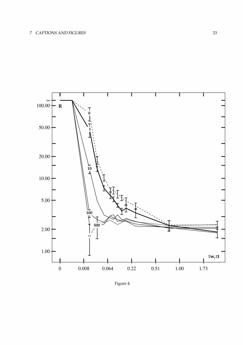
Figure 4 shows how variation of these parameters influences the overall performance of the diurnalpaddler.

FIGURE 4 ABOUT HERE.Paddlers were tested in a ramp background illumination regime with Ê max # � »y, lu¯ x . This is an

intermediate value where the Weber-machine is in its adaptation range at the bright end of the ramp. Onaverage, the paddlers experienced a background illumination of �@Óc½ � » lu¯ x . The time-constant .C� of theWeber machine was varied between .C�?#Þ, and .0�ß# � º ¸ . The time-constant .0/ of the ON/OFF channelswas covaried with .C� . (see the caption to figures 4a and 4b for more details)

At the low end of the .C� scale, the average background response is zero, so ¥à# + . For higher .�and .0/ , the foreground response increases due to memory effects. The background response increasesfaster so ¥ drops. Decreasing the strength of lateral inhibition (i.e. higher $ values) reduces the contrast-enhancement, and increases the sensitivity to global luminance fluctuations. Both effects result in a lower¥ . In all cases, the decrease of ¥ levels off above a certain .s� respectively $ value. For the lowest .C� ,adaptation in the ON/OFF channels can be so fast that the transient responses to temporal variations aretoo short to measure. If in that case there is no lateral inhibition ( $ # + ), the paddler is effectively blind,and ¥ is not defined (the dotted trace for $ # + in figure 4a starts only at .s�á#�,~º , � » ). Here, the averagedifference between the normalised eye-responses (

²) is zero (not shown). In the other cases,

²increases

with increasing .0� ; longer delays in adaptation (more memory effects) cause more and more unequalresponses in the two eyes.

²also increases with $ , which causes a larger sensitivity to variations in

background illumination. When the time-constants become too long, a target projection moving over theretina leaves an increasingly intense set of after-images, which are counted as background response; ¥decreases). An ”after-image” in the ON/OFF channel is in fact the 2nd derivative of the luminance input,the Weber-response taking a 1st derivative. Therefore, an ON luminance step results in a ON response,followed by a (longer) OFF response. Judging from direct observations of the retinal activities, the effectof after-images is especially strong for target-projections moving at high speed across the retina. Evencontrast-enhancement by lateral inhibition is no longer of any help: the cross-connections cause a lateralspreading of the after-image to the two neighbour cartridges.

How do these changes in vision work out on the foraging performance as indicated by � ? We find adecreasing performance with increasing .C� and $ that eventually levels off. An exception are of coursethe blind paddlers without any lateral inhibition ( $ # + ) and very short time-constants: these have a

4 EXPERIMENTS AND RESULTS 10

very low performance, as is evident from figure 4b. It can also be seen that increasing the time-constantsin these paddlers ameliorates their performance somewhat ( ¥ increases; cf. figure 4a). due to increasinglyintense after-images, performance stops increasing (and ¥ decreases) when the time-constants becometoo long. It is to be expected that for time-constants still larger than our upper value, performance willalso degrade.

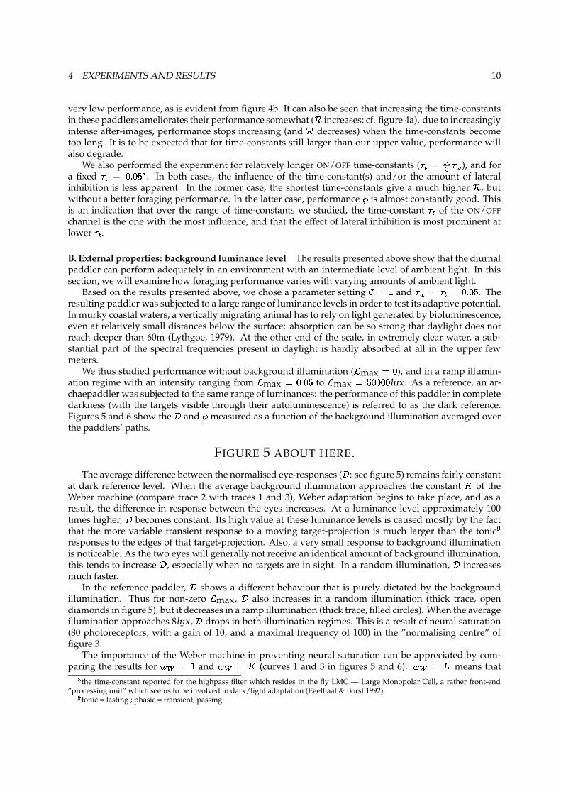
We also performed the experiment for relatively longer ON/OFF time-constants ( ./�# � «� .0� ), and fora fixed .0/�#â,~º�,�»yã . In both cases, the influence of the time-constant(s) and/or the amount of lateralinhibition is less apparent. In the former case, the shortest time-constants give a much higher ¥ , butwithout a better foraging performance. In the latter case, performance � is almost constantly good. Thisis an indication that over the range of time-constants we studied, the time-constant ./ of the ON/OFFchannel is the one with the most influence, and that the effect of lateral inhibition is most prominent atlower .0/ .B. External properties: background luminance level The results presented above show that the diurnalpaddler can perform adequately in an environment with an intermediate level of ambient light. In thissection, we will examine how foraging performance varies with varying amounts of ambient light.

Based on the results presented above, we chose a parameter setting $ # � and .s��#%.0/�#%,~º�,�» . Theresulting paddler was subjected to a large range of luminance levels in order to test its adaptive potential.In murky coastal waters, a vertically migrating animal has to rely on light generated by bioluminescence,even at relatively small distances below the surface: absorption can be so strong that daylight does notreach deeper than 60m (Lythgoe, 1979). At the other end of the scale, in extremely clear water, a sub-stantial part of the spectral frequencies present in daylight is hardly absorbed at all in the upper fewmeters.

We thus studied performance without background illumination ( Ê max #ä, ), and in a ramp illumin-ation regime with an intensity ranging from Ê max #�,pº�,�» to Ê max #�»�,@,�,@, lu

¯x. As a reference, an ar-

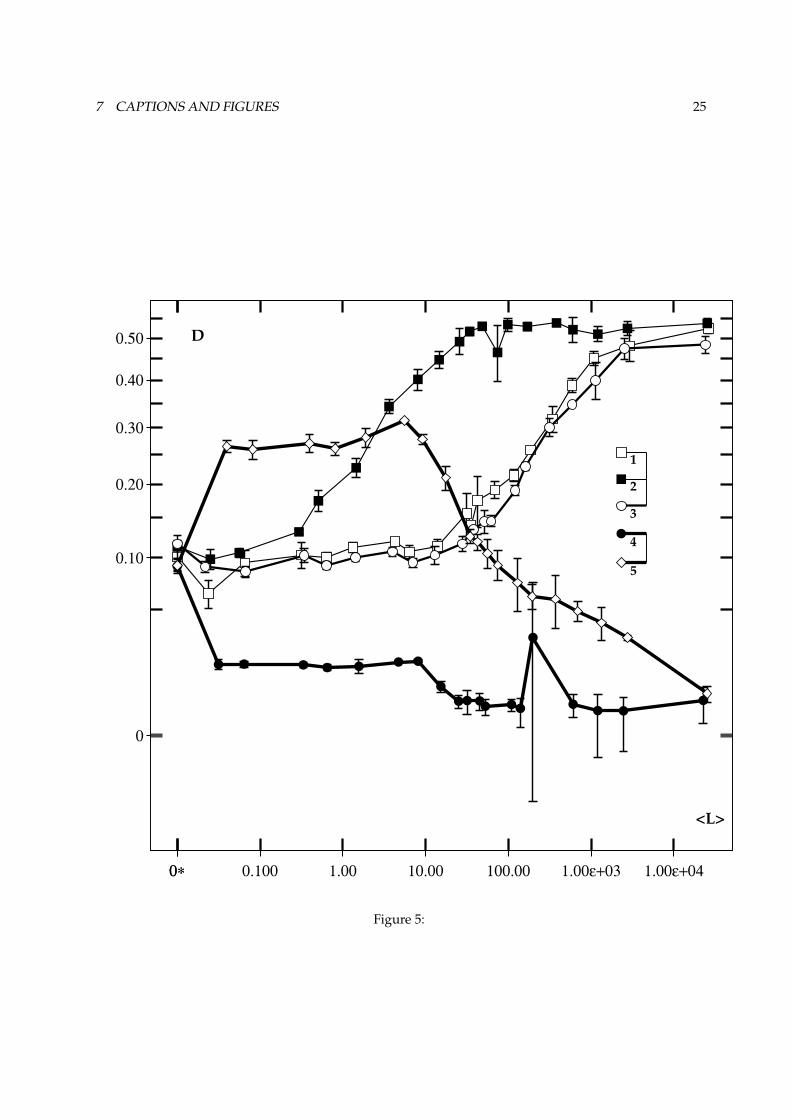
chaepaddler was subjected to the same range of luminances: the performance of this paddler in completedarkness (with the targets visible through their autoluminescence) is referred to as the dark reference.Figures 5 and 6 show the

²and � measured as a function of the background illumination averaged over

the paddlers’ paths.


The average difference between the normalised eye-responses (²

: see figure 5) remains fairly constantat dark reference level. When the average background illumination approaches the constant f of theWeber machine (compare trace 2 with traces 1 and 3), Weber adaptation begins to take place, and as aresult, the difference in response between the eyes increases. At a luminance-level approximately 100times higher,

²becomes constant. Its high value at these luminance levels is caused mostly by the fact

that the more variable transient response to a moving target-projection is much larger than the tonic åresponses to the edges of that target-projection. Also, a very small response to background illuminationis noticeable. As the two eyes will generally not receive an identical amount of background illumination,this tends to increase

², especially when no targets are in sight. In a random illumination,

²increases

much faster.In the reference paddler,

²shows a different behaviour that is purely dictated by the background

illumination. Thus for non-zero Ê max,²

also increases in a random illumination (thick trace, opendiamonds in figure 5), but it decreases in a ramp illumination (thick trace, filled circles). When the averageillumination approaches 8lu

¯x ,²

drops in both illumination regimes. This is a result of neural saturation(80 photoreceptors, with a gain of 10, and a maximal frequency of 100) in the ”normalising centre” offigure 3.

The importance of the Weber machine in preventing neural saturation can be appreciated by com-paring the results for d��æ# � and d��æ#çf (curves 1 and 3 in figures 5 and 6). d��æ#èf means thaté

the time-constant reported for the highpass filter which resides in the fly LMC — Large Monopolar Cell, a rather front-end”processing unit” which seems to be involved in dark/light adaptation (Egelhaaf & Borst 1992).ê

tonic = lasting ; phasic = transient, passing

5 DISCUSSION 11

the theoretical fully adapted state of the Weber machine equals the maximal firing frequency; a sufficientincrease in illumination would then cause saturation. Yet this does not happen to a significant degree.

The separation index ¥ (which decreases for Ê max ë , ) also levels off when²

becomes constant. Itsfinal value is still between 3 and 5 times higher than that of the reference paddler.


Finally, let us look at the foraging performance: see figure 6. The diurnal paddler performs at refer-ence level for all but the higher background luminances, where a slight drop can be observed. At thoseluminances, the background increasingly controls the paddler’s manoeuvres. Note that the much earlieronset of Weber adaptation for fì# �� d��í# � does not result in significantly worse performance. On theother hand, performance is worse ( � is significantly lower than its ”ideal” value 1) at low luminances forfî# � ,@, and ��# � . Here information is lost due to an insufficient gain in the Weber machine.

C. Decrement detection: effect of the OFF channels How is the above picture altered by assigninga non-zero weight to the OFF channels? To answer this question, we repeated the experiments withd � #�d # � . This means that both ON and OFF channels have equal votes in the paddler’s visually-guided behaviour.

The most significant effect is that the responses to both foreground and background illuminationare more or less doubled. In some cases, like fï#�dð�ñ# � , this causes a small increase in the fore-ground/background separation ( ¥ ) for the higher background luminance levels. However, ¥ decreasesfor zero background illumination: a result of after-images in the OFF channels. These effects do not resultin significantly different overall performance ( � ).

A clearer effect can be found for other combinations of the time-constants and the amount of lateralinhibition. For strong lateral inhibition (low $ ) and small time-constants, ¥ increases with respect to thecase d � #%, , while it decreases for lower lateral inhibition and/or higher time-constants. These effectsare also visible in the overal performance. They can be explained by a stronger (respectively weaker) tonicresponse to the edges of target-projections, which provide a more solid foundation for visual decisionsamidst the much more variable transient responses.

5 Discussion

We have studied simple visually-guided foraging in a diurnal environment. Ambient light provides ameans for detecting targets (from reflection), but it also introduces the need to ”discount the background”in phototaxic foraging. A mechanism is needed to distinguish object illumination from background illu-mination and to do this reliably over a wide range of background intensities. We therefore borrowed theideas of Weber adaptation and lateral inhibition from the literature on vision research and studied thequestion whether one of them or both together suffice(s) to solve the problem of object segregation undera wide range of ambient light intensities. At a given level of ambient light, we find a rather large rangeof time- constants and lateral inhibition ratios for which adequate (”near-optimal”) behaviour results,both in terms of foreground/background segregation at the retinal level, and in terms of the paddler’sforaging performance. In general, we find that performance is best for short time-constants, and a smalllateral inhibition fraction. The latter means that the ON/OFF channel compares the centre of its recept-ive field to a measure of the activity in its entire receptive field, where the surround weighs at least asmuch as the centre. As a result, the paddler effectively detects the edges of targets only. Edges (”spatialvariations”) give rise to a tonic response. Low time-constant values mean that both filters in the adapt-ing system respond to changes with minimal delay, and do not ”smear out” events in time. Temporalvariations thus give rise to a short transient response.

With weak lateral inhibition (large lateral inhibition ratios), only short to very short time-constantsgive rise to adequate performance. With no lateral inhibition at all, more temporal integration is needed,and mediocre performance results at best for long time-constants. The importance of lateral inhibitioncan best be seen at intermediate levels of background illumination, where the Weber machine’s transitionfrom a passive scaler to an adaptive scaler takes place. In this range, lateral inhibition is crucial to filter out

5 DISCUSSION 12

global luminance information that would otherwise get through. For stronger background illumination,the Weber machine’s response becomes transient, responding only to the changes in retinal illuminationcaused by target projections moving across the retina. In short, dark/light adaptation in this model isbest when local changes are detected with respect to (more) global constancy. In this way, the presenceof a target can be detected against the background. Using this well-known principle, we find that overa substantial range of ambient light levels, foraging performance can be on a par with the performanceof an archaepaddler in its own habitat (the dark reference, defined in the introduction). The limits ofthis range of good performance depend on the scaling constant and on the gain of the Weber machine.The scaling constant defines a level of input above which the Weber machine makes a transition from apassive filter (scaling with a constant) to an active, adaptively scaling filter.

A high ambient light level can cause large responses in the ON and/or OFF channels. A large scalingconstant will then result in better performance. However, depending on the gain, the Weber machine’soutput might in that case become sub-threshold for low levels of ambient light, or complete darkness, res-ulting in sub-optimal performance. Therefore a large scaling constant with a low gain may be beneficialfor life at very high luminance levels, but becomes a handicap at lower light levels. On the other hand,too low a scaling constant is suboptimal since adaptive scaling can then be initiated too soon. This meansthat no efficient use is made of the nervous system’s bandwidth, and that precious information can getlost. A compromise must (and can) be found between these two extremes if hunting is necessary both athigh and at low background levels. With the given model, detection of prey is possible over a wide rangeof ambient light levels, using just one type of photoreceptors. This range can be tuned to the paddler’sneed by adjusting just 3 parameters of the light adapting system (where the two parameters of the Webermachine can have identical values). In this way, paddlers that live in absolutely dark to (moderately)light environments can make do with the same mechanism that allows survival in moderately light tovery bright environments.

An interesting finding is that a dark/light adapting system with the best foreground / background se-gregation does not necessarily warrant the best foraging performance. Optimal foreground/backgroundseparation for intermediate levels of ambient light occurs e.g. for small time-constants, without lateralinhibition. Yet in that case performance is very bad, being solely based on blind search: all visual inform-ation is filtered out so fast that visual guidance of the behaviour is impossible. On the other hand, goodperformance can result within a range of foreground/background response ratios ranging from as lowas approximately 5 up to values several orders of magnitude higher. Similarly, the OFF channel does notcontribute to the information carried by the ON channel in such a way that it significantly improves over-all performance. For some settings, performance is even worse! Therefore, given the task of detectingobjects reflecting ambient light, it seems better not to use OFF channels. This changes, of course, if darkobjects (intercepting ambient light) become important either as prey or as predator. It therefore appearsthat OFF channels find their use exclusively in that realm.

A side-effect of dark/light adaptation by the present mechanism is that prey are detected by theiredges only. This means that size information, indicating distance to, or ”electability” of the prey, is nolonger present in terms of the total light response. With the current simple foraging strategy, this is nota problem, but it can become problematic when more elaborate foraging strategies arise. In that caseit is necessary to process contrast and edges rather than merely ”light” information. In principle, sizeinformation can be retrieved by a matching of the edges and comparing their local sign value, or bypropagating neural activity (”filling in”) inside matched edges. In the present 2D implementation of themodel, i.e. with a 1D retina, correct matching of the edges is problematic. In a 2D retina belonging to a3D model, the edges belonging to one target can in principle form a closed (elliptic) pattern of activityand thus be lumped. This would lead to a kind of silhouette vision. Rather then going in this directionof more sophisticated object analysis it would seem to be more profitable for foraging success to betteranalyse where objects are and where they are going. Anything of the proper size that can be hunteddown can then be tasted or courted. The same ON/OFF channels of the above system can be connected ina different way to form retinal image motion detectors similar to those reported in the fly (Franceschini1989, Egelhaaf and Borst 1992, 1993). Such elementary motion detectors are a necessary condition forextracting information from the optic flow, such as information on speed and direction of egomotion, andtime to contact to external objects. Paddlers with such enhanced capabilities of visual analysis will bedescribed elsewhere.

6 APPENDIX 1: A FORAGING PERFORMANCE MEASURE, � 13

From the above findings it is clear that the visual sytem should be tuned to the task and environmentin order to reach satisfactory performance. This emphasises the need for an approach to vision as de-scribed in this paper, where a complete perception-action cycle is studied rather than the visual systemin isolation. The parameters of the visual system might depend more strongly on the requirements ofinteracting with the world than on requirements to optimally ”see” the world.

Given this insight, it is interesting to note that another way to study such dependencies is by use of(unsupervised) evolutionary methods, e.g. genetic algorithms. Presently, efficient techniques for ”cod-ing” neural networks in genomic information are becoming readily available (e.g. Gruau 1994). Thismakes it feasible to embark on this kind of studies (see e.g. Beer & Gallagher 1992 or Cliff et al. 1993),which can provide unexpected new results. It should be noted, however, that the parametric studiespresented in this paper will continue to be useful to analyse the results (e.g. those in Cliff et al. 1993) ofsuch unsupervised evolution. Just as the result of natural evolution...

6 Appendix 1: a foraging performance measure, òOne performance measure might be the path choice efficiency. If the minimal total distance that has to betravelled to optimally fill the stomach is � min, and the actual total distance travelled to reach this goalis � t, then the ratio �Kó�# � min £ � t is obviously a measure of the path choice efficiency, where optimalperformance leads to �Kóõô � .

Now a paddler that only optimises path choice efficiency might not serve its goal of quickly fillingits stomach optimally. If it could reach the same end state with fewer prey of larger size it might bebetter off. However, the influence of target size does not show up in ��ó . This is so, since both � min and� t increase with the number of eaten targets, irrespective of their size. The ratio is about constant forincreasing numbers of (smaller) prey that are visited with the same navigation efficiency. Thus we needan additional factor for target choice efficiency, �"/ , which can be defined in an obvious way as the ratio ofthe average caloric value (’size’) of the eaten prey, 1*¡ � 2 , over the average caloric value (’size’) of all preypresent at the beginning of foraging, 1�¡@¢X2 . Thus ��/ð#±1*¡ � 2 £ 1�¡y¢02 . Again an optimal target choice wouldtend to lead to ��/�ô � . An overall performance factor � can be defined as the product of ��ó and ��/ , andthus takes both path choice and prey choice into account.

Of all mentioned terms, � min is the most problematic, since its calculation requires that we solvethe Travelling Salesman Problem, a feat of which we are not capable without putting constraints on theglowball population. To approximate � min for any given glowball population, we therefore resort toa simpler strategy. First we estimate the average �W�7�õ of all distances to the most profitable next targetfrom the position of each prey (”eating positions”), in a way described below in algorithmic fashion. Thenwe approximate � min as the product of the number of eaten prey during the whole foraging run and this(estimated) average minimal distance: � min # �ö� &p��3�\ . Taken together, this means that we define theperformance index as shown in formula 5 of the main text.

To account for changes in the prey distribution during foraging (e.g. as a result of eating), �W�7�\ and1�¡�¢X2 are updated at regular intervals during a simulation.The average minimal distance �W�7�õ in a prey distribution is determined by an algorithm that takes

information from both the prey distribution (caloric value & distance) and the paddler’s capabilities (itsfield of view) into account. To account for variations in the prey distribution, � �7� is calculated severaltimes during each simulation run. In the following pseudo-code description, ¬ stands for the number oftimes �Æ�7�õ has been calculated in the current run.

1. if n == 0, then total distance = 0 and segments = 0.

2. take a target, A, from the population, � .

3. if A is known to be the ”nearest of” to another target, C, then the orientation of an observerP moving from C to A is defined, and thus P’s field of view, ÷ , can be taken into account. (Thisinformation is not available for all targets during the first run on a new population (n == 0), andmay be outdated when the target distribution changed.)


4. find a target, B, among all other targets (including C) which compromises between a minimal cost(distance(A to B)) and a maximal reward (caloric value; size times luminance of the tar-get): minimise distance/reward. If ÷ is defined, also find the target B* with minimal dis-tance/reward and visible by P (within ÷ ).

5. if a target B* has been found, then B = B*.

6. tell A that, from its position, the most profitable next target is B:A->nearest to = B.Also tell B that it is A’s ”nearest to” target:B->nearest of = A.Update total distance and the number of segments:total distance += distance(A to B) ; segments += 1.

7. repeat from 2 for all targets in � .

8. update �W�3�\ and the counter n:�W�7�õ # total distancesegments ; n += 1.


Acknowledgements

The research presented in this paper was part of a PhD project of the first author supported by a grantfrom the Foundation for Biophysics (presently Foundation for the Life Sciences) of the Netherlands Or-ganisation for the Advancement of Scientific Research (NWO).

We thank dr. A. Noest and dr. M. Lankheet for critically reading the manuscript, and the BioInform-atics department (Prof. P. Hogeweg) for the use of their workstations.


References

Beer R.D. (1990) Intelligence as Adaptive Behavior - An Experiment in Computational Neuroethology.Boston, Academic Press 1990

Beer R.D. and Gallagher J.C. (1992) Evolving Dynamical Neural Networks for Adaptive Behavior. Ad-aptive Behavior 1 1992: 91-122

Bertin R.J.V. (1994) Natural smartness in Hypothetical animals-Of paddlers and glowballs, PhD thesis

Bertin R.J.V. and van de Grind W.A. (1996) Phototropic foraging in the archaepaddler, a hypotheticaldeep-sea species. Submitted for publication.

Bouman M.A., van de Grind W.A. and Zuidema P. (1985) Quantum fluctuations in vision. In: Wolf W.(ed): Progress in Optics Vol. XXII. North-Holland, Amsterdam 1985: 39-144

Braitenberg V. (1984) Vehicles - Experiments in Synthetic Psychology. Cambridge, MA, The MIT Press1984

Cliff D. and Bullock S. (1993) Adding ”Foveal Vision” to Wilson’s Animat. Adaptive Behavior 2 1993:49-72

Cliff D., Husbands P. and Harvey I. (1993) Explorations in Evolutionary Robotics. Adaptive Behavior 21993: 73-110

Corbacho F.J. and Arbib M.A. (1995) Learning to Detour. Adaptive Behavior 4 1995: 419-468

Cruse H., Brunn D.E., Bartling Ch., Dean J., Dreifert M., Kindermann J. and Schmitz J. (1995) Walking:A Complex Behavior Controlled by Simple Networks. Adaptive Behavior 4 1995: 385-418

Dennett D.C. (1995) Darwin’s dangerous idea. Simon & Schuster, New York 1995

Egelhaaf M. and Borst A. (1992) Are there seperate ON and OFF channels in fly motion vision?. Vis.NeuronSci. 8 1992: 151-164

Egelhaaf M. and Borst A. (1993) Motion computation and visual orientation in flies. Comp. Biochem.Physiol. 104A 1993: 659-673

Ekeberg O., Lansner A. and Grillner S. (1995) The Neural Control of Fish Swimming Studied ThroughNumerical Simulations. Adaptive Behavior 4 1995: 363-384

Franceschini N., Riehle A. and le Nestour A. (1989) Directionally Selective Motion Detection by InsectNeurons. In: Stavenga & Hardie (eds.): Facets of Vision. Berlin/Heidelberg, Springer-Verlag 1989: Ch.17, 360-390

Gibson J.J. (1979) The ecological approach to visual perception. Houghton Mifflin Company, Houston

van de Grind W.A., Koenderink J.J. and Bouman M.A. (1970) Models of the Processing of Quantum Sig-nals by the Human Peripheral Retina. Kybernetik 6 1970: 213-227

van de Grind W.A. (1990) Smart mechanisms for the visual evaluation and control of self-motion. In:Warren R & Wertheim A (eds.): Perception and control of self-motion. Hillsdale NJ, LEA: Ch. 14, 357-398

Gruau F. (1994) Automatic Definition of Modular Neural Networks. Adaptive Behavior 2 1994: 151-183

Hartline H.K. and Ratliff F. (1974) Studies on excitation and inhibition in the retina. Chapman and Hall,London

Koenderink J.J., van de Grind W.A. and Bouman M.A. (1970) Models of Retinal Signal Processing at HighLuminances. Kybernetik 6 1970, 227-237

Kuhn, A (1919) Die Orientierung der Tiere im Raum. Gustav Fischer Verlag, Jena 1919


Loeb J. (1918) Forced movements, tropisms and animal conduct. Philidelphia, Lippincott 1918; repub-lished 1973, Dover, New York

Lythgoe J.N. (1979) The ecology of vision. Oxford, Clarendon Press, 1979

Rossler O.E. (1974) Adequate locomotion strategies for an abstract organism in an abstract environment-A relational approach to brain function. In: Conrad M., Guttinger W. and Dal Cin M. (1974): Lecture Notesin Biomathematics 4: Physics and Mathematics of the Nervous System. Berlin/New York, Springer Verlag1974: 342-370

Simmons P.J. (1993) Adaptation and responses to changes in illumination by second- third-order neur-ones of locust ocelli. J. Comp. Physiol. 173: 635-648

Shapley R.M. and Enroth-Cugell C. (1984) Visual adaptation and retinal gain controls. Progress in retinalresearch 3 1984: 263-346

Terzopoulos D., Tu X., and Grzeszczuk, R. (1994) ”Artificial Fishes with Autonomous Locomotion, Per-ception, Behavior, and Learning in a Simulated Physical World. In: Brooks R. and Maes P. (eds.):Artificial Life IV: Proc. of the Fourth International Workshop on the Synthesis and Simulation of LivingSystems. Cambridge, MA, 1994: p.17-27

Walter W.G. (1950) An imitation of life. Scien. Am. 182: 42-45

Walter W.G. (1951) A machine that learns. Scien. Am. 185: 60-63

7 CAPTIONS AND FIGURES 18

7 Captions and Figures

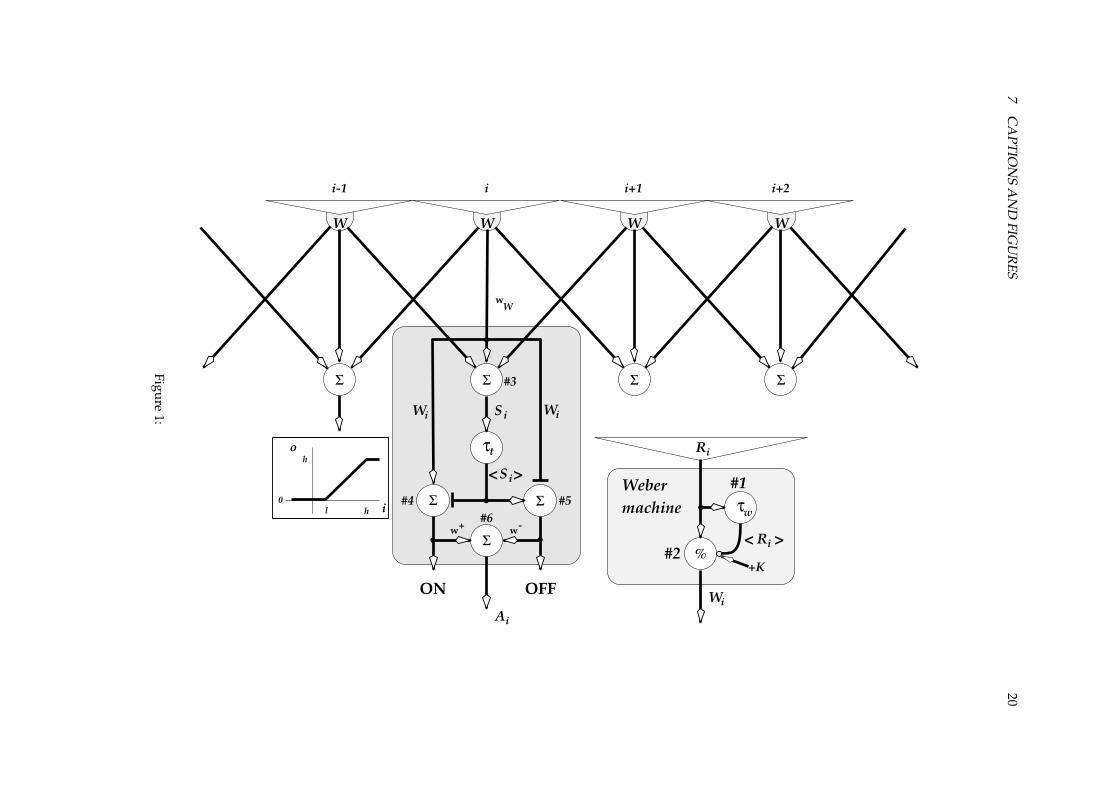
Figure 1 :The diurnal paddler’s retina. A lateral inhibition layer feeds ø�ùÇúsû cartridges, each containing a Weber machine

working on a weighted sum of ON and OFF channels. ü : a ”normal” excitatory connection; ý�ý0þ : an inhibition; ý�ý(ÿ :a shunting inhibition (here with the scaling constant � ). �� is used to indicate a dividing neurone; �

�indicates a

summator; ��

a multiplier and ��

a leaky integrator. The photoreceptors have a gain of 10.0. The white box shows theclipping function performed by all cells: �Kù��Xû� � and gù��Xûsû .Figure 2 :

The paddler’s anatomy. The two eyes were placed at a position of �Çù �sû�� , sampling an angle of ��rù��û�� ,centered around the eye-axis at �ßù��sû�� . Light absorption by the water was approximately 0.125 lu

¯x/m

¯and the

direction of optimal sensitivity was at an angle ��5ý�� !� ú � to the eye-axis. Thus the effective visual horizon was at� �Üù"��# m¯

, and �%$ ù&�'# m¯

. The inset shows a screendump of an actual paddler, in which all proportions are correct.Negative angles indicate clockwise rotations. Values given are for the left eye: for the right eye, multiply angles by -1.

Figure 3 :Visuomotor network of the diurnal paddler’s nervous system.The weighted sums of the (*) responses (2 times ø )

from the left and right eye are projected onto respectively the right and the left paddles, after having been normalisedand temporally averaged by leaky integrators. In the absence of visual information, searching behaviour is generated(circuit not shown). Weighting of the ( ) responses is Gaussian, with a halfwidth +¾ù&�-,�� centered around ��ùßý�� !� ú��(see figure 2), and height .%/ . Individual (%) responses from the binocular field receive an additional weight-factor0 ù_û � , . Clipping parameters as in figure 1.

Figure 4a :1as a function of 243 and 5 .The average foreground/background ratio as a function of the lateral connection

weights and the (coupled) time-constants with �àù6� ûsû , .7/�ù6� ûû and 2�8ðù92 3 , for a ramp illumination regimewith a luminance range of 150. Performance is ideal for 2 3;: û � ûsû�� . Performance progressively decreases withincreasing 5 and increasing 2 3 ; in both cases, the decrease of

1saturates. Numbers in the curves indicate the 5

values; error-bars indicate standard deviations..

Figure 4b :< against 2 3 and 5 .Performance as a function of the lateral connection weights and the (coupled) time-constants

with � ù=�Xûsû and .>/äù?� ûsû , for a ramp illumination regime with a luminance range of 150. Performance is best forlow 2 3 and low 5 . Note that for 5�ù;@ (only the central photoreceptor’s output is used), the paddlers perform in amediocre way at best, for higher 2 3 only. In this case, the tonic response due to spatial filtering is absent. Thereforealmost all visual information is discarded (the paddlers are ”in search mode” almost constantly), except for the larger243 values which introduce their own disadvantages. Numbers in the curve indicate the 5 values; error-bars indicatestandard deviations.

Figure 5 :Aagainst average background illumination,measured during a simulation similar to the one in figure 4. All diurnal

paddlers shown here remain close to the reference performance of an archaepaddler at B max ù�û for at least afraction of the range of illuminations that were experienced. For average background illuminations approaching � ,Weber adaptation occurs. This is visible as an increase in

A. Neurones saturate at a firing level of 100 (spikes per

timestep). 2 3 ù"2C8�ùÚû � û-, , 5¾ù=� . Trace 1: � ù=� ûsû�DE.%/äù=� ; trace 2: � ù".>/äù=� ; trace 3: � ù".>/äù=� ûû ; trace4: reference paddler, ramp illumination; trace 5: reference paddler, random illumination. Error-bars indicate standarddeviation.

Figure 6 :< against average background illumination;performance measured during the simulation shown in figure 5. It is

clear to see that performance of all diurnal paddlers remains on the dark reference level for the complete range ofbackground illuminations, despite the increase in

Avisible in figure 5. Note that, at low background illumination,


when it can still more or less separate targets from the background, the archaepaddler performs better in a rampregime. However, at high background illumination, performance is somewhat better in a random regime. Now thedistraction of the randomly changing background completely guides the paddler, preventing it from swimming instraight paths. Error-bars indicate average of the standard deviation of each curve. Trace 1: � ù�� ûû DE.*/Þù�� ; trace2: ��ùF.>/ ù?� ; trace 3: ��ùG.>/�ù?� ûû ; trace 4: reference paddler, ramp illumination; trace 5: reference paddler,random illumination. Error-bars indicate standard deviation.

7C

APT

ION

SA

ND

FIGU

RES

20

W

w

Σ

-

Σ

+

Σ

w

Σ

Σ

τ

%iR< >

iW

>

τ<

Σi

W

S

W

i

W

S

W

wW

iA

iR

Σ #5

iWi

ON OFF

t

i-1 i i+1 i+2

l h0

ho

i w

+K

Webermachine

#1

#2

#3

#4#6

Figure1:

7C

APT

ION

SA

ND

FIGU

RES

21

paddle

β

α

ε

ϕv

Dv

binocular field

εD

tailfin

Figure2:


i=1 i=N.................................. ..................................

%

{

τ

(1+ϖ)

τ

<A>L <A>R

weight

Normalisation

iA iA

ς

ε

σ

binocular

Σ

ε

to

left

paddle

to

right

paddle

σ ς

%

Figure 3:


τw,τtτw,τt1.00

2.00

5.00

10.00

20.00

50.00

100.00∞

0 0.008 0.064 0.22 0.51 1.00 1.73

R

τw,τt

Web,Fτw=1 C=0 Web,Fτw=1 C=1 Web,Fτw=1 C=10 Web,Fτw=1 C=100 Web,Fτw=1 C=500 Web,Fτw=1 C=∞

rp

0

1

10

100

∞

500

Figure 4:


τw,τtτw,τt0.15

0.25

0.35

0.45

0.55

0.65

0.75

0.85

0.95

1.05

0 0.008 0.064 0.22 0.51 1.00 1.73

℘

τw,τt

Web,Fτw=1 C=0 Web,Fτw=1 C=1 Web,Fτw=1 C=10 Web,Fτw=1 C=100 Web,Fτw=1 C=500 Web,Fτw=1 C=∞

rp

∞

500

10010

0

1

Figure 4b


<L><L>

0

0.10

0.20

0.30

0.40

0.50

0∗0∗ 0.100 1.00 10.00 100.00 1.00ε+03 1.00ε+04

D

<L>

1

2

3

4

5

Figure 5:


<L><L>0

0.20

0.40

0.60

0.80

1.00

1.20

0∗0∗ 0.100 1.00 10.00 100.00 1.00ε+03 1.00ε+04

℘

<L>

1

2

3

4

5

Figure 6:

The inuence of light/dark adaptation and lateral ... · The inuence of light/dark adaptation and...

Documents

Transcript of The inuence of light/dark adaptation and lateral ... · The inuence of light/dark adaptation and...