THE IMPACT OF FARM MECHANIZATION ON SMALL-SCALE RICE PRODUCTION

THE IMPACT OF FARM MECHANIZATION ON SMALL-SCALE RICE PRODUCTION

Y OLANDA L . TAN

MASTER OF SCIENCE ( A g r i c u l t u r a l Economics)

M a r c h , 1981

THE IFPACT OF FARM MECHANIZATION ON SMALL-SCALE RICE PRODUCTION

YOLANDA L. TAN

SUBMITTED TO THE FACULTY OF THE GRADUATE SCHOOL UNIVERSITY OF THE PHILIPPINES AT LOS BmOS

IN PARTIAL FULFILLMENT OF THE REQUIREMENTS FOR THE

DEGREE OF

MASTER OF SCIENCE ( A g r i c u l t u r a l E c o n o m i c s )

March, 1981

The thesis attached hereto entitled: THE IMPACT OF FARM

MECHANIZATION ON SMALLeSCALE RICE PRODUCTIONp prepared and

submitted by YOLANDA L. TAN, in partial fullfillment of the

requirements for the degree of Master of Science (Agricultural

Economics), is hereby accepted:

BART DUFF' Member. Guidance Committee Member, Guidance Committe

f l . /- TIRSO B. PARIS, Adviser and Chairman Guidance Committee

3 - & r P / (Date)

Accepted as partial fullfillment of the requirements for

the degree of Master of Science (Agricultural Economics).

DOLORES A. RAMIREZ Dean, Graduate School

University of the Philippines at Los Ba5os

BIOGRAPHICAL SKETCH

Yolanda L. Tan was born in San Pablo City, Laguna on

October 17, 1956. She finished her high school education in

1974 at the Laguna College in San Pablo City. In the same

year, she was awarded the local State Scholarship grant to

pursue undergraduate studies at the University of the Philip-

pines at 1.0s Baiios. She finished her college education in

1978 with the degree of Bachelor of Science in Statistics.

After graduation, she joined the Commerce Department's

teaching staff of the Laguna College. In 1979, she was granted J'

an IAPMP (Integrated Agricultutal Productivity and Marketing

Program) Fellowship to pursue a Master's degree in Agricul-

tural Economics at the University of the Philippines at Los

Bafios. For her thesis work, she was awarded a partial sholar-

ship by the International Rice Research Institute as a Research

scholar. Presently, she is an instructor in the Economics

Department of the College of Development Economics and Manage-

ment, UP at Los Baiios.

iii

ACKNOWLEDGEMENT

My most s i n c e r e g r a t i t u d e and profound app rec i a t i on t o

my adv i se r s : D r . Bar t Duff, Assoc ia te A g r i c u l t u r a l Economist

a t t h e I n t e r n a t i o n a l Rice Research I n s t i t u t e (IRRI), D r . T i r s o

B. P a r i s , Jr., Chairman and Ass i s t an t P ro fe s so r , College of

Development Economics and Management (CDEM), Univers i ty of t h e

P h i l i p p i n e s a t Los Bafios (UPLB) , and D r . Corazon T. Aragon,

College Sec re t a ry and Ass i s t an t P ro fe s so r , CDEM, UPLB f o r t h e i r

c o n s t r u c t i v e c r i t i c i s m and guidance i n t h e p repa ra t i on of t h i s

t h e s i s .

S i m i l a r g r a t i t u d e and app rec i a t i on a r e a l s o extended t o

D r . Paul G. Webster, V i s i t i n g A g r i c u l t u r a l Economist a t I R R I ,

D r . John A. Wicks, Assoc ia te A g r i c u l t u r a l Economist a t I R R I

and D r . Hans P. Binswanger, former A g r i c u l t u r a l Development

Council (ADC) Assoc ia te f o r I n d i a , f o r t h e i r va luable he lp i n

c l e a r i n g important d e t a i l s of t h e methodol~gy of t h e t h e s i s .

To t h e I n t e g r a t e d A g r i c u l t u r a l P r o d u c t i v i t y and Marketing

P r o j e c t f o r p rovid ing a fe l lowship t o pursue a Mas te r ' s degree

i n A g r i c u l t u r a l Economics a t UPLB.

To t h e I n t e r n a t i o n a l Rice Research I n s t i t u t e f o r providing

a p a r t i a l t h e s i s suppor t .

Warm thanks t o my roommates, Jerome and Precee, f o r t h e i r

good company and he lp i n t h e p repa ra t i on of t h e d a t a used i n

t h i s t h e s i s .

To t h e S e c t i o n ' s programmers, Murphy, Edi th and Al i ce ,

who helped i n t h e process ing of t h e d a t a , our s e c r e t a r i e s ,

Lydia and Hedda f o r t h e i r e x c e l l e n t typ ing job and my col-

leagues a t t h e Economics s e c t i o n of t h e A g r i c u l t u r a l Depart-

ment, F leur , Rigs , Mely, Bardz and C e l l i e , who made my s h o r t

s t a y a t I R R I f r u i t f u l and enjoyable .

To Meyra, Pur ing and t h e rest of my c lassmates f o r

s h a r i n g wi th me t h e hard times and good t imes of ou r course

works.

And l a s t l y , t o my pa ren t s and b ro the r s , whose love ,

encouragement and moral support se rved me i n s p i r a t i o n t o

complete my graduate work.

TABLE OF CONTENTS

CHAPTER PAGE

I INTRODUCTION . . . . . . . . . . . . . . . . . . 1

. . . . . . . . . . . . . . . . . . 1.1 Problem 1

1 .2 Objectives . . . . . . . . . . . . . . . . 3

1 .3 Hypothesis . . . . . . . . . . . . . . . . 3

I I REVIEW OF LITERATURE . . . . . . . . . . . . . . 6

2 . 1 History of the Growth of Farm Mechanization in the Philippines . . . . . . . . . . . . 6

2.2 Related Literature on Production Effects . . . . . . . . . . . . . of Mechanization 8

2.3 Survey of the Literature on Decomposition Analysis . . . . . . . . . . . . . . . . . 11

I11 RESEARCH METHODOLOGY . . . . . . . . . . . . . . 17

3 . 1 Decomposition Model I (Arithmetic Decomposition Technique) . . . 17

3.2 Decomposition Model I1 (Employing the Use of Production Function Framework) . . . . . . . . . . . . . . . . 24

3.3 SourceofData . . . . . . . . . . . . . . . 3 1

3 .4 Sampling Procedures . . . . . . . . . . . . 32

IV STUDY AREA AND CHARACTERISTICS OF SAMPLE FARMS . 3 4

4 .1 Study Area . . . . . . . . . . . . . . . 34

4.2 Characteristics of Sample Farms . . . . . . 36

. . . . . . . . . . . . . V RESULTS AND DISCUSSION 41

5 .1 Results of the Arithmetic Decomposition . . . . . . . . . . . . . . . . . . . Scheme 4 1

CHAPTER PAGE

5.2 R e s u l t s of t h e Decomposition Scheme Using t h e Produc t ion Funct ion Framework . . . . . . . . . . . . . . . . 59

SUMMARY ANDCONCLUSION . . . . . . . . . . . . 70

LITERATURE CITED . . . . . . . . . . . . . . . . . . . . . APPENDIX I 76

. . . . . . . . . . . . . . . . APPENDIX 11 80

. . . . . . . . . . . . . . . . . . APPENDIX 111 82

APPENDIXIV . . . . . . . . . . . . . . . . . 83

. . . . . . . . . . . . . . . . . . APPENDIX V 84

TABLES

LIST OF TABLES

PAGE

D i s t r i b u t i o n of Sample Farms by Mun ic ipa l i t y . . . and B a r r i o , Nueva E c i j a , P h i l i p p i n e s , 1979 3 5

D i s t r i b u t i o n of Sample Farms by Type of Power Used i n Land P r e p a r a t i o n and I r r i g a t i o n , Nueva E c i j a , P h i l i p p i n e s , Wet Season, 1979 . . . . . . 37

Demographic C h a r a c t e r i s t i c s of Sample Farms by Type of Mechanizat ion, Nueva E c i j a , P h i l i p p i n e s , Wet Season, 1979 . . . . . . . . . . . . . . . 3 8

C h a r a c t e r i s t i c q of Sample Farms by Type of Mecha- n i z a t i o n , Nuevn E c i j a , P h i l i p p i n e s , Wet Season, 1 9 7 9 . . . . . . . . . . . . . . . . . . . . . 39

Tes t f o r D i f f e r ences of Va r i ab l e s Between T r a c t o r and Carabao Farms Using t h e Kruskal-Wallis One- Way Analys i s of Variance by Ranks . . . . . . . 42

Means of Var.iables Used i n Applying t h e Ar i th - me t i c Decomposition Analys i s , Wet Season, 1979

. . . . . . . . . . . . . and Dry S'eason, 1980 4 4

Decomposition Analys i s (Without I n t e r a c t i o n Terms) of Output D i f f e r ences Between 2-wheel T r a c t o r and Carabao Farms . . . . . . . . . . 45

Decomposition Analys i s (Without I n t e r a c t i o n Te~rns ) of Output D i f f e r ences Between 2-wheel T r a c t o r and Carabao Farms w i t h P r i c e Va r i ab l e . 4 5

Decomposition Analys i s (With I n t e r a c t i o n Terms) of Output D i f f e r ences Between 2-wheel T r a c t o r and Carabao Farms . . . . . . . . . . . . . . . 4 6

Decomposition Analys i s (wi th I n t e r a c t i o n Terms) of Output D i f f e r ences Between 2-wheel T r a c t o r and Carabao Farms w i t h P r i c e Var iab le . . . . . 4 7

Decomposition Analysis (Without I n t e r a c t i o n Terms) of Outnut D i f f e r ences Between 2-wheel/ 4-wheel T r a c t o r Combination and Carabao Farms 5 1

PAGE TABLE

12 Decomposition Analysis (Without I n t e r a c t i o n Terms) of Output Di f fe rences Between 2-wheel/ 4-wheel Trac tor Combination and Carabao Farms wi th P r i c e Variable . . . . . . . . . . . . 51

Decomposition Analysis (With ' ~ n t e r a c t i o n Terms) of Output Di f fe rences Between 2-wheel/4-wheel

. . . . Trac to r Combination and Carabao Farms 52

Decomposition Analysis (With I n t e r a c t i o n Terms) of Output Di f fe rences Between 2-wheel/4-wheel T r a c t o r Combination and Carabao Farms wi th P r i c e

. . . . . . . . . . . . . . . . . . . Variable 53

Cropping I n t e n s i t y of Sample Farms by Type of Power Used i n Land Prepara t ion and I r r i g a t i o n , Wet Season, 1979, Dry Season, 1980 . . . . . . 5 6

Cropping I n t e n s i t y of Sample Farms by Type of Power Used i n Land Prepara t ion and I r r i g a t i o n , Wet Season, 1979, Dry Season, 1980 . . . . . . 58

Estimated Coef f i c i en t s of t h e Cobb-Douglas Product ion Function f o r t h e 2-wheel T rac to r

. . . . . . F a r m s . . . . . . . . . . . . . . 60

Estimated Coef f i c i en t s of t h e Cobb-Douglas . . . Production Function f o r t h e Carabao Farms 61

Estimated Coef f i c i en t s of t h e Cobb-Douglas Production Function f o r t h e 2-wheel/4-wheel T r a c t o r Combinat ion Farms . . . . . . . . . . . 62

Test f o r S t r u c t u r a l Di f fe rences i n t h e Produc- t i o n Functions f o r 2-wheel T rac to r and Carabao Farms Using t h e Dummy Var iab le Approach . . . 65

Means of Var iab les Used i n Applying the Decom- pos i t i on Analysis Using the Production Function Framework, Wet Season, 1979. . . . . . . . . . 67

Decomposition Analysis of Per Hectare Yield Dif fe rences Between 2-wheel Trac tor and Carabao Farms . . . . . . . . . . . . . . . . . . . . 68

APPENDICES

APPENDIX PAGE

. . . . . . . . . . . I Mathemat ica l I d e n t i t i e s

1 . I d e n t i t y I . . . . . . . . . . . . . . . . . 2 . I d e n t i t y I1 . . . . . . . . . . . . . . .

3 . I d e n t i t y 111 . . . . . . . . . . . . . . I I The Kruskal -Wal l i s T e s t . . . . . . . . . . .

. . . . . . . . . I11 Mathemat ica l Trans fo rmat ion

I V N i t r o g e n Content o f Organic and Commercial F e r t i l i z e r s . . . . . . . . . . .

. . . . . . . . . . . . . . V The Chow's T e s t

ABSTRACT

TAN, YOLANDA L . , U n i v e r s i t y of t h e P h i l i p p i n e s a t Los

Bafios, March 1981. The Impact of Farm Mechanizat ion on Small-

s c a l e Rice Produc t ion . T h e s i s a d v i s e r : D r . B a r t Duff .

The o b j e c t i v e of t h i s s t u d y i s t o q u a n t i t a t i v e l y a s s e s s

t h e impact of farm mechanizat ion on o u t p u t . P roduc t ion e f f e c t s

of mechanizat ion were e v a l u a t e d through t h e u s e of decomposi t ion

a n a l y s e s . F i r s t , an a r i t h m e t i c decomposi t ion a n a l y s i s was

employed t o d i s a g g r e g a t e o u t p u t d i f f e r e n c e s between mechanized

and non-mechanized farms i n t o i t s component e l e m e n t s , i . e . , , .

y i e l d , p r i c e , a r e a and c ropp ing i n t e n s i t y component p l u s t h e

i n t e r a c t i o n s of t h e s e components. R e s u l t s of t h e a n a l y s i s

showed t h a t t h e most impor tan t f a c t o r s t h a t brought abou t

o u t p u t d i f f e r e n c e s between t h e mechar~ized and non-mechanized

farms were c ropp ing i n t e n s i t y and y i e l d .

Secondly, y i e l d e f f e c t of mechanizat ion was i n v e s t i g a t e d

by u s i n g a n o t h e r decomposi t ion t echn ique employing a p roduc t ion

f u n c t i o n framework. The model decomposed t o t a l y i e l d d i f f e r e n c e s

between t h e mechanized and nan-mechanized farms i n t o t h e techno-

l o g i c a l change component and change i n t h e u s e of i n p u t s com-

ponent . The r e s u l t s of t h e a n a l y s i s showed t h a t t h e major

s o u r c e of y i e l d d i f f e r e n c e s between t h e e . 7 0 farm t y p e s WAS

brought about by non-neutral technical change, i . e . , s h i f t

i n the slope coef f i c i ents of the production functions, which

means differences in the a l locat ion of resources of the two

farms.

CHAPTER I

INTRODUCTION

Technological advancement is one of the important forces

which alters the production structure of a growing economy. The

significance of technological change is that it permits continuous

improvement in the productivity of resources by the constant flow

of innovations and skills for resource utilization. Technological

changes may call for readjustments of resources employed in the

agricultural sector relative to the other sectors of the economy.

New technology, therefore disturbs the equilibrium of the recei-

ving environment and can result in a chain of complex technical,

economical, social, cultural and institutional effects that are

neither easily predictable nor necessarily consistent with the

aims of rural development.

1.1 Problem

The term "technical change" means broadly any change

relevant to productivity growth and is commonly accepted as

basic to any meaningful policy for economic development of the

agricultural sector. Analyzing, therefore, the effects of'the

existing technologies will help to effectively improve and

tailor new technological possibilities to the needs of rural

development.

2

Mechanization of small farms, as a form of technical

change in developing countries, is frequently equated with

modernization. Faced, therefore, with a growing rural labor

force and increasing demand for food, the development, intro-

duction and use of agricultural machines in LDCs had produced

a large and controversial literature describing technical, eco-

nomic, socio-anthropological attempts to quantify, measure and

evaluate the impact of mechanization on farm output, employment

and income distribution. For example, there appear too few

rigorous studies which demonstrate conclusively and convincingly

the net effect of mechanical techniques, This study, therefore,

will try to measure quantitatively and analyze the output effects

of mechanization.

Farm mechanization has been the center of a continuing con-

troversy for many decades now, The focal point of these debates

11 centers around five major issues:-

1. does mechanization increase farm productivity (yield/

hectare and yield/hectare/year] if so, how?

2 . to what degree is labor displaced by machines and what

are the alternative employment opportunities for that displaced

l/~he Consequences of Small Rice Farm Mechanization on Pro- duction, Incomes and Rural Employment in Selected Countries of Asia (A Project Proposal), IRRI, February 1978.

3 labor?

3. to what extent are the benefits of mechanization con-

centrated in the better endowed sectors of the rural society?

4. with the rising prices of fuel energy, is it still

economical to mechanize?

5. what policies should the government follow to obtain

the desirable benefits of mechanization while minimizing the

undesirable effects?

1.2 Objectives

Given the five major farm mechanization issues, this study

will address itself only to the first one. It aims to develop

a methodology to resolve bhe question of whether mechanization

increases output or not. This will be done by analyzing the

effects of mechanization on output using decomposition analysis

which will partition total observed output differences between

mechanized and non-mechanized farms into the factors that brought

about such differences.

1.3 Hypotheses

Mechanization as an input, holding water availability and

seed variety constant could be investigated as to whether it

increases output or not. Evidence from Thailand (Inukai, 1970),

Nepal (Thapa, 1979) and Philippines (Antiporta and Deomamapo, 1979)

showed t h a t ou tpu t from mechanized farms was h ighe r than non-

mechanized farms. The observed d i f f e r e n c e s i n ou tpu t between

t h e s e farms could be due t o t h e d i f f e r e n c e s i n y i e l d , a r e a cult-

t i v a t e d and cropping i n t e n s i t y of t h e two farm types .

With r e s p e c t t o ou tpu t d i f f e r e n c e s a t t r i b u t e d t o mechaniza-

t i o n , t h e fo l lowing hypotheses were t e s t e d :

1. The adopt ion of farm machinery i n c r e a s e s y i e l d ho ld ing

a l l o t h e r i n p u t s cons t an t .

2 . Mechanization i n c r e a s e s cropping i n t e n s i t y .

Output d i f f e r e n c e s between mechanized and non-mechanized farms

could a l s o be due t o changes i n t h e f a c t o r s o f p roduc t ion o r

i n p u t s used and a s h i f t i n technology. I n t h i s s t u d y , t e c h n i c a l

change was taken t o mean mechanizat ion of small r i c e farms.

The impact of t e c h n i c a l change could be decomposed i n t o two

components: (1) an e f f i c i e n c y component ( n e u t r a l t e c h n i c a l

change) i . e . , more ou tpu t could be produced under t h e new produc-

t i o n technology w i t h t h e same level of i n p u t s , and (2) an a d j u s t -

ment component (non-neutra l t e c h n i c a l change) i . e . , t h e e f f o r t s

o f fa rmers t o r e a l l o c a t e t h e use of i n p u t s a t t h e new level of

e f f i c i e n c y . Th is s tudy l i kewi se sea rched f o r t h e sou rce s of

ou tpu t d i f f e r e n c e s between mechanized and non-mechanized farms.

S p e c i f i c a l l y , i t t e s t e d t h e fo l lowing hypotheses:

3. The ou tpu t d i f f e r e n c e s between mechanized and non-mecha-

nized farms are due to neutral technical change ox incxeesed

efficiency in production.

4 . The output differences between these two farm types

are brought about by non-neural technical change which implies

reallocation in the use of inputs in the production processes.

CHAPTER I1

REVIEW OF LITERATURE

This section surveys the literature on the history of the

growth of farm mechanization in the Philippines, production

effects of mechanization and the decomposition techniques used

by various authors as a method for the component analysis of

output growth.

2.1 History a£ the Growth of Farm Mechanization in the Philippines

Agricultural mechanization in the Philippines began as

early as in the final years of the Spanish period with the impor-

tation of disc harrows, cultivators, gang-plows and corn planters

(Santos, 1946). At the end of World War I (1918), tractor mecha-

nization was mainly concentrated on large sugar cane plantations,

although large mechanical stationary threshers powered by four-

wheel and crawler tractors were repozted to have been introduced

and used during the late 1930's. After World War I1 (19461, with

the government efforts to foster mechanization through the exemp-

tion of farm machinery imports from custom duties, special import

taxes and countervailing duties (Piputsitee, 1976), the country

was able to import an average of 650 tractors annually (Follosco,

1966). These machines coming from the industrialized countries

were, however, considered i n e f f i c i e n t and c o s t l y because they

were b a s i c a l l y developed f o r d i f f e r e n t condi t ions of e i t h e r

l a r g e farm hold ings and higher l abo r c o s t s as i n t h e United

S t a t e s , o r f o r subs id ized small farms a s i n Japan which was f a r

from the agro-economic s i t u a t i o n of t h e country. A s a r e s u l t ,

farm mechanization was i n s i g n i f i c a n t p r i o r t o 1960. Another

reason f o r t he slow adoption of farm mechanization during these

yea r s was t h e country had a su rp lus of a g r i c u l t u r a l l and , hence

a g r i c u l t u r a l production could be increased through t h e opening

of new land and increased use of necessary inpu t s . But wi th t h e

c los ing of t h e land f r o n t i e r during t h e 1960's, a s i g n i f i c a n t

s h i f t i n resource use i n a g r i c u l t u r e took p l ace , r equ i r ing inno-

v a t i o n s t h a t would r e s u l t t o i nc rease i n land p roduc t iv i ty o r

y i e l d per hec t a re (Crisostomo and Barker, 1972).

A census of farm machinery d e a l e r s i n 1960 r epor t ed t h a t

50% of t h e 8,500 t r a c t o r s i n t he country were owned by t h e l a r g e

sugar farmers , 35% by r i c e farmers and 15% by o t h e r crop farmers

(Almario, 1979). This r e l a t i v e l y high t r a c t o r use by sugar f a r -

mers during the y e a r s 1962-64 could be r e l a t e d t o t h e sugar in-

dus t ry boom r e s u l t i n g from che United S t a t e s embargo placed on

Cuban sugar imports r e s u l t i n g i n higher p r i c e s f o r P h i l i p p i n e

sugar (Duff, 1975).

I n t h e l a t e 1960, t h e r e was increased t r a c t o r mechaniza-

t i o n e s p e c i a l l y i n r i c e production brought about by t h e govern-

ment's adoption of credit programs and the advent of high yiel-

ding varieties which raised'fam incomes and improved investment

potentials for mechanical technology. Concurrently, power tillers

or hand tractors were introduced primarily for land preparation.

In 1965, the International Rice Research Institute (IRRI)

initiated a USAID funded research and development program to

produce a range of small low cost machine designs which would

enhance the production possibilities of small rice farmers. The

goal was to develop equipment which could be manufactured and

maintained locally, and which could be within the investment

capabilities of farmers with landholdings of 2 tb 5 hectares.

After fifteen years of research and development, a number

of IRRI designs have entered commercial production, At present,

IRRI together with the private manufacturers of farm machineries

are attempting to strengthen further the research and development

programs for agricultural mechanization tailored to the needs of

small rice fanners in Asia (McMennamy, 1976).

2.2 Related Literature on Production Effects of Mechanization

The use of farm machineries in less developed countries

presents two opposing views. On the one hand, farm mechanization

allows a faster, less laborious and timely operations of farm

tasks which is claimed to lead both to increased yields and

g r e a t e r i n t e n s i t y of land use . It is a l s o argued t o i n c r e a s e

l a b o r p r o d u c t i v i t y and income,

On t h e o t h e r hand, i t is o f t e n seen a s a d i r e c t s u b s t i t u t e

f o r l abo r which i s undes i r ab l e i n p l aces wi th ex t ens ive l a b o r

supply, o f t e n t h e ca se of less developed coun t r i e s . Agricul tu-

r a l mechanization, however, may supplement, s u b s t i t u t e o r comple-

ment o t h e r f a c t o r s i n t h e product ion process (Duff, 1978) depen-

ding on t h e type of machines used.

It could be a s u b s t i t u t e f o r l a b o r and animal power a s i n

t h e c a s e of t r a c t o r s ; a supplement, a s i n t h e ca se of r o t a r y

weeders, f e r t i l i z e r a p p l i c a t o r and in sec t i c ide lweed ic ide sp raye r s ;

and a complement a s i n t h e ca se of i r r i g a t i o n pumps i n r a i n f e d

a r e a s .

Product ion e f f e c t s of mechanization could be viewed i n terms

of cropping i n t e n s i t y , cropping p a t t e r n and y i e l d e f f e c t s . I n a

2 1 review of t r a c t o r s t u d i e s i n I n d i p , cropping i n t e n s i t y was

h igher on t r a c t o r farms than t h e bu l lock farms i n 30% of t h e

ca se s reviewed. This i n t e n s i t y advantage of t r a c t o r farms was

no t n e c e s s a r i l y caused by t r a c t o r i z a t i o n s i n c e most of t h e ca se s

which repor ted increased cropping i n t e n s i t y was observed t o be

/ ~ i n s w a n ~ e r , H. .Economics of T rac to r s i n South A s i a , ADC, New York and ICRISAT, Hyderabad, Ind i a , 1978, pp. 19-3Q.

paralleled with improved irrigation facilities. Thexefore, the

studies reviewed, taken together, gave little support to the hypo-

thesis that tractorization is an important factor in increasing

cropping intensity.

In the case of cropping pattern, an impressive advantage

31 was observed from these studies- for tractor farms. Further

analysis, however, showed that this was also due to variety of

facrors other than tractorization, such as access to capital and

water availability. In a recent study of Pate1 (1980), the order

of priority of crops studied in the cropping pattern of tractor

and bullock farms in Gujarat, India was the same. This implied

that cropping pattern was not affectd by the tractorization of

the farms.

Yield advantages of tractor farms appeared to be large in more

than 50% of the studies cite$! However, in most of the reported

cases, fertilizer use was also higher in the tractor farms. This

higher yield in the tractor farms, therefore, was not exclusively

due to tractorization.

Assessing the existing studies and researches on tractoriza-

tion in less developed countries, the tractor surveys resulted to

3 1 Ibid., pp. 42-47 -

4 1 Ibid., pp. 30-37 -

inconclusive evidences that tractors are responsible for signi-

ficant increases in cropping intensity, yields, cropping patterns

and gross returns on farms. There is, therefore, a need to quanti-

tatively measure the impact of tractorization on output, employment

and income distribution to conclusively evaluate the net effects

of mechanical techniques.

2.3 Survey of the Literature on Decomposition Analys-is

Decomposition analysis or component analysis is a mathemati-

cal technique for partitioning an aggregate into its component

elements. Early studies have applied the decomposition technique

to investigate the effects of technological change on output

growth (Solow, 1957), an important factor that received attention

in the earlier literature. In this pioneering work of Solow, a

geometric productivity index was presented, which was a substan-

tial refinement over the previous arithmetic index of Abramovitz

(1956).

The Solow index was formally derived from a general production

function. Assuming perfect competition, the process tried to

measure technological change by decomposing output growth into

explanatory components which are actually changes in inputs used,

i.e., capital and labor, weighted by their respective factor

shares and a residual term which was a measure of technical

change.

Decomposition analysis was likewise used to allocate diffe-

rences in productivity resulting from a variety of factors such

as the extension of cultivation to new areas due to reclamation

of virgin land and deforestation, and increases in cropping in-

tensity made possible by the spread of irrigation and adoption

of better crop rotations (Minhas and Vaidyanathan, 1965).

The component analysis of output growth used for the first

time by Minhas and Vaidyanathan was an additive scheme of decom-

position. Change in aggregate output was decomposed into four

components, i.e., the contribution of:

a. changes in area

b. changes in per acre yield

c. changes in cropping pattern

d. the interaction between yield and

cropping pattern

The Minhas-Vaidyanathan framework is one of the several

additive methods of decomposition analysis. In addition to the

additive schemes, one can also decompose output into different

component elements in a multiplicative fashion. The results

obtained, however, from the multiplicative decomposition scheme

are not as easy to interpret as in the additive scheme. This

framework involved interaction terms of component elements which

mean simultaneous effects of the components.

More recent studies have used decomposition techniques for

decomposing output growth in Gujarat (Misra, 1971) and for a

comparative analysis of the pre-Green Revolution periods in

India (Sonhdi and Singh, 1975). Both studies used a slightly

modified version of the original Minhas and Vaidyanathan model

in so far as an interaction term between area and other components

was added.

Decomposition analysis was also used to quantify the employ-

ment effects of technical change (Krishna, 19741, which was taken

to mean changes in water availability, cropping intensity, seed

varieties, fertilizer use and the degree of mechanization. The

model was used to decompose total labor input into:

a. irrigation effect

b. variety effect

c. tractor-ploughing effect

d. irrigation technology effect

e . threshing effect

f. interaction effects of irrigation

and varietal improvement

The framework allowed for the grading of each individual tech-

nical change according to the magnitude of its positive and

negative employment effects.

Output growth was further investigated by Sagar (1977)

who tried to decompose overall productivity of crops into a price

effect, yield effect, cropping pattern changes and the interac-

tions of these components. Narain (1977) also used a framework

similar to that of Sagar, only it was more specific with respect

to crop types and for different states.

Another decomposition technique was used by Bisaliah (1977)

in analyzing factors affecting output growth, this time using a

production function framework. He decomposed the total chang?

in yield due to the introduction of new production technology

into the proportion brought about by technical change and the

proportion due to the change in the input levels.

Bisaliah (1978) also employed a decomposition technique to

evaluate the total employment effects of technical change. Using

a labor demand function derived through a unit-output-price

profit function, the total change in employment between new and

old technology farms was decomposed into:

a. a technology component

b. a wage rate component, and

c. a complementary inputs component.

Binswanger (1978) presented a decomposition technique that

disaggregated output growth into cropping intensity, yield,

cropping pattern effects and an R-term. The R-term, which is

15

actually the residual term, was regarded simply as approximation

errors arising out of the switch f r m the continuous function

to the discrete formulation.

Rathore (1979) verified Binswanger's decomposition scheme

by using the model to disaggregate total observed differences

in output between small and large farms. The analysis resulted

in large, unacceptable residuals and another decomposition

model without residual was suggested (Binswanger, 1979).

Assessing the literature on deconnposition analysis, little

has been done to evaluate output and employment differences

that might result from mechanization.

Decomposition analysis is one of the many methodologies

that can evaluate the effects of mechanization on production

(Binswanger, 1978) and employment (Krishna, 1974). The tech-

nique could be designed to allocate the observed output and

employment differences between farms "begore and after" or "with

and withoutf' certain machines into the following component ele-

ments viz. cropping intensity, yield, cropping pattern and

price. This partitioning shows the relative importance of com-

ponent effects, thus enabling the analyst to identify the most

fruitful areas for further investigation.

The decomposition technique may be an arbitrary scheme,

but at the back of it is an analytical design (Minhas and Vaid-

yanathan, 1965). In this scheme component elements, i.e.,

cropping i n t e n s i t y , cropping p a t t e r n , y i e l d and p r i c e are

chosen and arranged i n a manner s u c h - t h a t t h e i r i nd iv idua l e f f e c t s

can be a d d i t i v e l y aggregated. Each f a c t o r can be s e p a r a t e l y

analyzed t o provide measures of output growth brought about by

t h e i r absolu te changes. This a l l o c a t i o n of output d i f f e rences

i n t o its component elements is u s e f u l i n providing guidance i n

i d e n t i f y i n g t h e important f a c t o r ( s 1 t h a t brought about such

output d i f f e rences . Together wi th t h e information about d i f fe ren-

ces i n i r r i g a t i o n , cropping p a t t e r n and modern package of tech-

nology l i k e HYV, f e r t i l i z e r s , p e s t i c i d e s , e t c . , a p i c t u r e of t h e

output e f f e c t s of a given machine can be constructed.

RESEARCH- ~ O D O M G Y

In evaluating whether mechanization increases output or

not, decomposition analyses was employed to explain the observed

output differences between farms "with and without " mechaniza-

tion in terms of its component elements,

3.1 Decomposition Model I

Output between mechanized and non-mechanized farms was

investigated and tested for differences using the Kruskal-Wallis

one-way analysis of variance by ranks2! Having shown that there

is a statistical difference in output between mechanized and

non-mechanized farms, an arithmetic decomposition technique was

employed. The goal of this decomposition method is to disaggre-

gate the difference in observed output between the two farm

types into its explanatory components, viz. yield, cropping

intensity, area and price. Since no attempt has ever been made

to examine'simultaneously the effects of these contributory

components to output growth due to mechanization and to quantify

their magnitudes together, this formulation was specifically

aimed to bridge this methodological gap.

z'~iegel, S. Nonparametric Statistics for the Behavioral Sciences, McGraw-Hill Kogakusha, Ltd., 1956, pp.184-193.

1 8

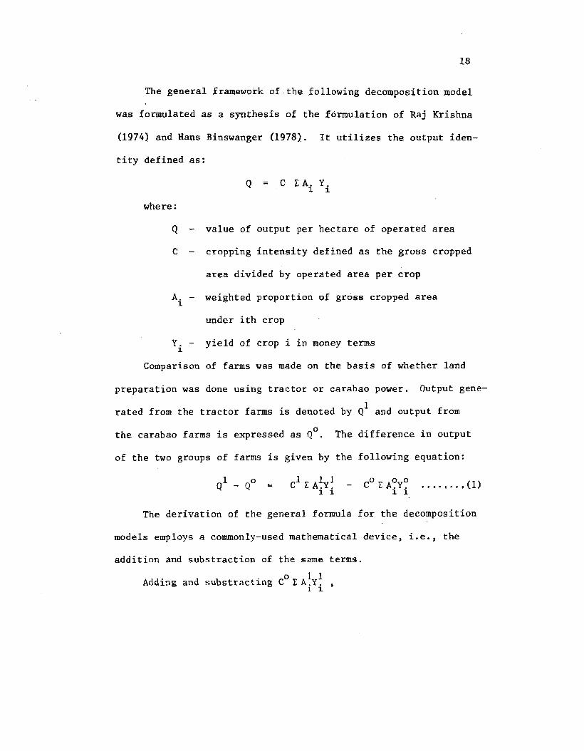
The g e n e r a l framework of t h e fo l lowing decomposit ion model

was formulated a s a s y n t h e s i s of t h e fo rmula t ion of Raj Krishna

(1974) and Hans Binswanger (19782. I t u t i l i z e s t h e ou tpu t iden-

t i t y de f i ned a s :

Q = C Z A i Y i

where :

Q - v a l u e of ou tpu t pe r h e c t a r e of opera ted a r e a

C - cropping i n t e n s i t y de f i ned a s t h e g r o s s cropped

a r e a d iv ided by opera ted a r e a p e r c rop

Ai - weighted p ropo r t i on of g r o s s cropped a r e a

under i t h c rop

'i - y i e l d of c rop i i n money terms

Comparison of farms was made on t h e b a s i s of whether l and

p r e p a r a t i o n was done u s ing t r a c t o r o r ca rabao power. Output gene-

1 r a t e d from t h e t r a c t o r farms i s denoted by Q and ou tpu t from

0 t h e carabao farms i s expressed a s Q . The d i f f e r e n c e i n ou tpu t

of t h e two groups of farms i s g iven by t h e fo l l owing equa t ion :

The d e r i v a t i o n of t h e g e n e r a l formula f o r t h e decomposit ion

models employs a commonly-used mathemat ical dev i ce , i .e . , t h e

a d d i t i o n and s u b s t r a c t i o n of t h e same terms.

1 1 Adding and s u b s t r a c t i n g CO E A . Y .

1 1 '

and c o l l e c t i n g common terms result i n :

1 0 Define t h e (C -C ) X A'Y' as component A and t h e i i

1 1 0 0 q u a n t i t y cO( I: AiYi - I: A.Y .) as component B. I n o r d e r t o s impl i -

1 1

f y t h e n o t a t i o n s , d i f f e r e n c e s i n ou tpu t , y i e l d , a r e a weight and

cropping i n t e n s i t y can now be w r i t t e n i n terms of d e l t a (A) such

t h a t ,

1 0 Q - Q = A Q A' - A0 = AA

C1 - C0 = AC Y1 - Yo = AY

Working f i r s t on component B and expanding i t by u s ing

I d e n t i t y I from Appendix I-A l e a d s t o :

The f i r s t term of Equat ion 4 is t h e cropping i n t e n s i t y

e f f e c t , t h e second term is t h e area effectk ' and t h e t h i r d term

i s t h e o v e r a l l y i e l d e f f e c t . Th i s fo rmula t ion is a c t u a l l y t h e

6' The second t e r n of Equation 4 i s a c t u a l l y t h e c ropping p a t t e r n e f f e c t i n t h e Binswanger model, bu t s i n c e t h e p r e s e n t model is designed f o r mono c rop ( r i c e ) p roduc t ion , i t n e c e s s a r i l y becomes an a r e a e f f e c t .

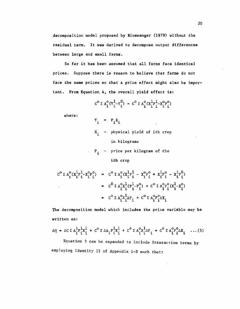
decomposition model proposed hy Binswanger (1979) without t h e

r e s i d u a l term. It w a s der ived t o decompose output d i f f e r e n c e s

between l a r g e and sma l l farms.

So f a r i t has been assumed t h a t a l l farms f a c e i d e n t i c a l

p r i c e s . Suppose t h e r e is reason t o b e l i e v e t h a t farms do no t

f a c e t he same p r i c e s s o t h a t a p r i c e e f f e c t might a l s o be impor-

t a n t . From Equation 4, t h e o v e r a l l y i e l d e f f e c t is:

where :

Xi - phys i ca l y i e l d of i t h crop

i n kilograms

- p r i c e p e r kilogram of t h e

i t h crop

The decomposition model which inc ludes t h e p r i c e v a r i a b l e may b e

w r i t t e n a s :

Equation 5 can be expanded t o i nc lude i n t e r a c t i o n terms by

employing I d e n t i t y I1 of Appendix I -B such t h a t :

Using Identity 111 from appendix^. to expand the parenthesized

expressions leads t o the f ina l decomposition equation:

Arranging the terms:

0 0 0 AQ = ACZAiPiXi - cropping intensity e f f ec t

0 0 0 + C ZAiPiAXi - pure yie ld e f f ec t

+ COCAA~P:X: - area e f fec t

0 0 + C L A ~ A P ~ X ! - price e f f ec t

first-order interaction terms

- second-order interaction terms

+ ACCAAiAPiAXi - third-order interaction term

This model is an extension of Binswanger's model without

residual. In the present formulation, interaction terms were

incorporated and treated as first-order, second-order and third-

order interaction effects of the contributory components. These

interaction effects indicate the influence.of any of the factors

over the other that brought about output differences between farm

types. The degree of the interaction terms expresses the number

of component elements that are allowed to change simultaneously

in the model. The first-order interaction terms will refer to

the simultaneous effects of the component elements taken two at

a time. The second-order interaction terms will mean three com-

ponents are changing simultaneously and the thirdwrder interac-

tion term reflects the simultaneous effect of all the four com-

ponents . To c l a r i f y t h e i s s u e of i n t e r a c t i o n e f f e c t s , an example i s

c a l l e d f o r . Take t h e ca se of t h e f i r s t - o r d e r i n t e r a c t i o n be t -

ween cropping p a t t e r n and p r i c e v a r i a b l e s . Th i s can be u s e f u l

i n f i n d i n g whether the nrowth i n g r o s s cropped area of a p a r t i -

c u l a r c rop i s due t o t h e r e l a t i v e p r o f i t a b i l i t y of t h e c rop

because of a f a v o r a b l e p r i c e i n t h e market o r n o t . Th i s can a l s o

be due t o a h ighe r p r o d u c t i v i t y l e v e l and t h e second-order i n t e r -

a c t i o n between y i e l d , p r i c e and cropping p a t t e r n would h e l p i n

unders tand ing t h i s . That i s , t h e r e l a t i v e p r o f i t a b i l i t y of t h e

crop brought about by i nc r ea sed p r o d u c t i v i t y and f a v o r a b l e p r i c e

i n t h e market would change t h e cropping p a t t e r n i n i t s f avou r .

Hence, t h e i n t e r a c t i o n of cropping p a t t e r n wi th p r i c e and y i e l d

can prov ide an i n s i g h t i n t o t h e p a t t e r n of crop ad jus tments

towards c rops w i t h h ighe r y i e l d o r w i t h h ighe r p r i c e , and t h e

second-order i n t e r a c t i o n e f f e c t of t he se t h r e e components can shed

some l i g h t on t h e a l l o c a t i o n of c u l t i v a t e d a r e a t o p a r t i c u l a r

c rops .

3.2 , DeCdmbpo~i,tiori 'Model I1

Previous studies (Elinhas and Vaidyanathan, 1965), (Sagar , 1977) showed that the most important source of output growth

associated with the introduction of new technology is yield. The

second part of this methodology outlines another decomposition

scheme that will disaggregate the difference in per hectare

paddy output into components brought about by technical change

(neutral and non-neutral technological change) and change in the

levels of inputs used.

The decomposition model involves the use of a production

function and is formulated specifically to answer the following

questions:

a. is there a difference in the structural form if the

production functions derived from mechanized and non-mechanized

farms, i.e., are the intercept and slope coefficients for mecha-

nized technology equal to the coefficients of the non-mechanized

technology?

b. if there is structural difference, is it due to changes

in the efficiency parameter (intercept) of the production function

or changes in the output elasticities (slope parameters) of the

inputs used, or both?

The fram2work is a revised model of Bisaliah (1977) emplo-

ying tl~e use of a Cobb-Douglas motlel. The production function

for mechanized farms is specsf ied as follows:

Similarly, the production function for non-mechanized farms

\ could be specified as follows:

where :

Y - yield per hectare of palay in kilograms

L - pre-harvest labor input per hectare measured as total

manhours used in planting, care and cultivation of

the crop except land preparation. These included

activities like seeding of. seedbed, pulling of seed-

lings, transplanting, irrigating, fertilizer appli-

cation, weeding and applying weedicide and insecti-

cide.

F - total amount of fertilizer used per hectare converted

to nitrogen in kilograms (see appendix 111)

C - total amount of crop protection used, i.e., pesticide,

insecticide, fungicide, herbicide, weedicide and roden-

ticide valued in pesos per hectare

/ P-- total amount of machine/animal services used in land

preparation measured in man-machine/animal hours per

1lec tare.

A - scale parameter

Br - output elasticities of inputs

for the mechanized farms

'i - output elasticities of inputs

for the non-mechanized farms

U and E - disturbance terms where: E = log U

M - mechanized farms

B - non-mechanized farms

L/~n decomposing the structural differences of the produc- t ion functions for the mechanized and the non-mechanized- farms, the variable P must be made comparable for both farms, since in the case of the mechanized farms, P is measured in terms of man- machine hours, while in the case of non-mechanized farms, P is in terms of man-animal hours. To make them comparable, man- machine hours were converted to equivaleqt man-animal hours by multipying a proportion which measure the speed of a particular type of tractor, i.e., 2-wheel or 4-wheel, over a carabao in preparing a hectare of land. This was done by comparing the average amount of machine hours needed to plow, harrow and level a hectare of land to the average amount of animal hours.

In the case of 2-wheel tractor farms versus carabao farms, the ratio of the speed of the tractor over the carabao in preparing a hectare of land is 3.3 (see Table 4). For the combination of 2-wheel/4-wheel tractor versus carabao farms, the ratio is 3.4. These values were therefore used to standardize P and hence made them comparable.

The production functions can be transformed into the

locarithmic form as follows:

log YM = log + B1log LM + B210g FM + B310g CM

log Y = log $ + Z1log LB + B log FB + B log CB B 2 3

+ B410gPB+EB . . . . . . . . . . . (41

The structural difference of the two production functions

was tested using the Chow's test .8' In case the statistical

test demonstrates or reveals significant differences between

the two sets of coefficients, the decomposition Model 11 was

then employed.

The decomposition model can be derived by taking the

difference of the predicted linearized production functions

for both mechanized and non-mechanized farms using average

values for each variables.

8'Chow, G.C., "Test of Equality Between Sets of Coefficients in Two Linear Regressions," Econornetrica, Vol. 28, No. 3. July, 1960, pp. 591-605.

Adding and subtracting some terms to (5) and rearranging

them results in:

rlr I, bog yM.- log yB1 = [log - log $1 + p1 - zl) log iB + A' A A A

(B2 - Z2) log PB + (B3 - Z3) log EB + h (G4 - z4) log F~]+ [sl (log - log ZB) +

A f i B2 (log SM - log P ) + B3 (log EM - log FBI +

B

,- B4 (log FM - log iB)1 + [EM - E~] . . . . (6)

Equation (6) could also be written as:

f i A n iog[q = [iOg [:I] + - zl) log iB + (B2 - z2) log rB +

A t. A ($3 - Z ) log cB + (B4 - Z4) log iiB +

3 I [i1 k\ + g2 log k] + s3 10. [$I R B4 10. [?]I+ & - . . . . • • • • • . . (7)

Using this decomposition scheme, the per hectare output

differences between mechanized and non-mechanized farms can be

decomposed into three components:

a. neutral technological change (i.e., shift in the

intercept of the production function)

b. non-neutral technological change (i.e., shift in the

slope parameters of the production function)

c. change in the volume of inputs used (i.e., labor,

fertilizer, crop protection and capital services)

The decomposition Model I1 approximates a measure of the

percentage change in output (Appendix 11) due to mechanization

holding all other factors like irrigation and seed varieties

constant. Equation (7) involves the disaggregation of the

natural logarithm of the ratio of output produced from mechan-

ized and non-mechanized farms. The first bracketed expression

on the right hand side, the natural logarithm of the ratio of

the intercept terms, measures the percentage change in output

due to neutral technological change. The second bracketed

expression, the sum of the arithmetic changes of slope para-

meters each weighted by the logarithm of the volume of the

particular input used, measures the percentage change in output

due to non-neutral technological change. The third bracketed

expression, the sum of the logarithms of the ratio of each

input used under mechanized and non-mechanized farms, each

weighted by the output elasticity of that input. measures the

percentage change in output due to changes in labor, fertilizer,

crop protection and capital services used. The fourth bracketed

expression is simply the measure of differences in error terms.

The decomposition models formulated in this section attempt

to assess the possible impact of mechanization on small rice

farms. They were designed to present a fairly complete picture

of the sources of output growth that can be attributed to

mechanization.

Drawbacks of these decomposition techniques are expected

to arise during the process of analysis. In the case of the

first model, i.e., the simple arithmetic decomposition scheme,

one of the limitations that can easily be pointed out is that

although it involves heavy (but simple) computational work, it

is wasteful of information because it does not use all the

available data due to aggregation. Another is that, it is

considered as an ad hoc method for analyzing the impact of

mechanization on production since no rigorous methodological

framework was involved in its formulation. It is purely an

accounting method. This does not, however, mean that the re-

sults are barren of significant interpretation. The manner

in which output growth was decomposed in the models are expected

to bring out the important factor(s) that are affected by

mechanization. The technique attempts to address the question

of the source of the major differences in output between the

mechanized and non-mechanized farms. This provides direction

in evaluating the impacts of mechanization on yield, cropping

intensity, cropping pattern and price, if they exist. It

leads one to ask precisely why such an effect arises and hence,

the possible source of the effect. Is mechanization responsible

for that effect or is it simply spurious?

The second model, i.e., the decomposition scheme using the

production function framework, is of course subject to ell the

possible limitations of a Cobb-Douglas formulation such as

least-squares bias, multicollinearity and specification errors.

The scheme, however, tries to answer questions raised from the

first decomposition model. It specifically presents the

component elements that are causal to the possible yield effects

of mechanization.

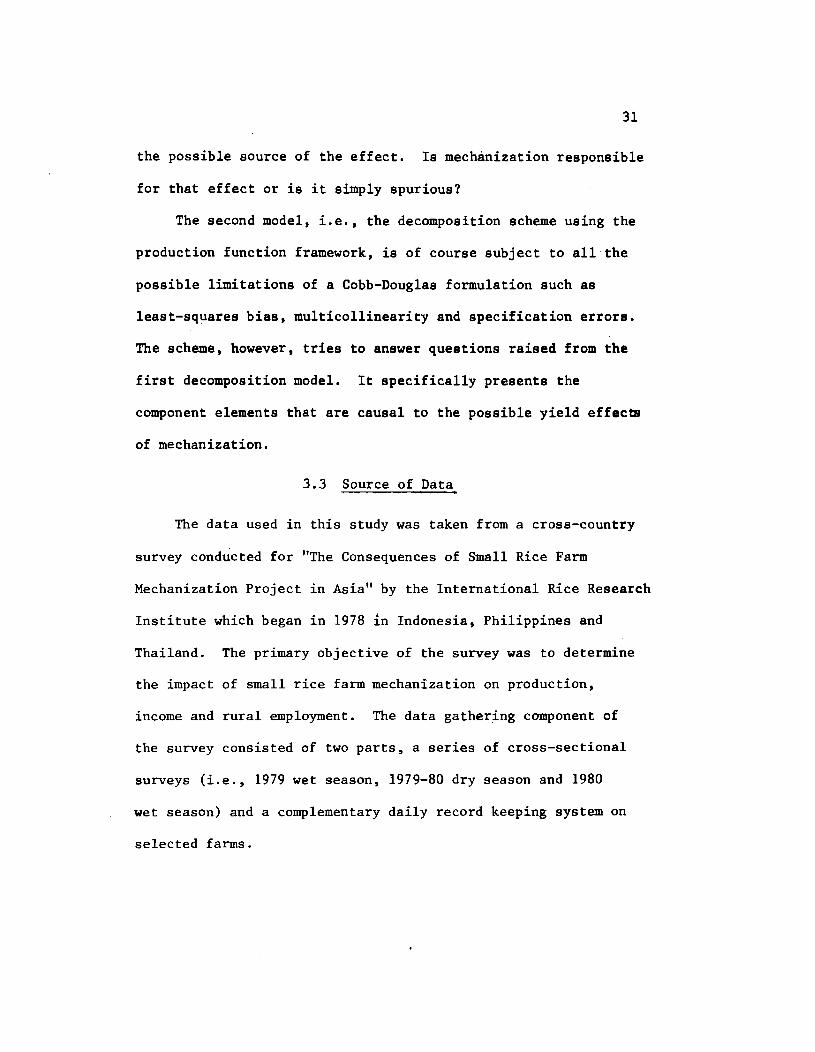
3.3 Source of Data

The data used in this study was taken from a cross-country

survey conducted for "The Consequences of Small Rice Farm

Mechanization Project in Asia" by the International Rice Research

Institute which began in 1978 in Indonesia, Philippines and

Thailand. The primary objective of the survey was to determine

the impact of small rice farm mechanization on production,

income and rural employment. The data gathering component of

the survey consisted of two parts, a series of cross-sectional

surveys (i.e., 1979 wet season, 1979-80 dry season and 1980

wet season) and a complementary daily record keeping system on

selected farms.

32

- 9 / 3.4 Sampling Procedures

A household census was administered at the beginning of

the study to identify the farm operators and landless field

laborers in each barrio. Data collected from the census was

used primarily in selecting the samples needed for the study.

Two municipalities which were primary rice producing areas

were purposively selected. Selection was based on the survey's

primary stratification criteria which are: the type and extent

of irrigation available and the degree of mechanization in land

preparation.

To select the sample households, stratified random sampling

was employed. The stratification based on the type of irriga-

tion and power used for primary tillage is as follows:

1. rainfed - animal power 2. rainfed - 2-wheel tractor 3. rainfed - 4-wheel tractor 4. irrigated, one cropping season - animal power 5. irrigated, one cropping season - 2-wheel tractor

6. irrigated, one cropping season - 4-wheel tractor 7. irrigated, two or more cropping season - animal power

)/Moran P. and Unson D. "Farm Survey and Recordkeeping Procedures for the Consequences of Small Rice Farm Mechanization Project: Operation Handbook" IRRI/USAID, May 1980.

33

8. i r r i g a t e d , two o r more cropping season - 2-wheel t r a c t o r

9. i r r i g a t e d , two o r more cropping season - 4-wheel t r a c t o r

10. l and le s s f i e l d l abore r s

The s t r a t i f i c a t i o n u n i t used i n the farm households was t h e

pa rce l and n o t t h e t o t a l farmholding. Pa rce l s loca ted ou t s ide

t h e sample b a r r i o s and those t h a t t o t a l l e d t o more than 10 hec-

t a r e s were excluded. The l a t t e r exclusion was due t o i t 8 s i z e

category which i s oute ide t h e d e f i n i t i o n of emall farm. In t h e

case of farmers wi th more than one p a r c e l , s t r a t i f i c a t i o n was

based on t h e pa rce l wi th the l a r g e s t a r e a planted t o r i c e . I f

the l a r g e s t pa rce l was loca ted ou t s ide the sample b a r r i o , t h e

l a r g e s t among pa rce l s w i th in the b a r r i o was chosen t o characte-

r i z e the t o t a l farmholding.

Af ter a l l the r i c e farm households and f i e l d labor house-

holds had been placed i n r e spec t ive s t r a t i f i c a t i o n c e l l s , 40

households were randomly drawn from each of t he f i r s t 9 s t r a t a ,

w i th t h e l a s t 5 households serv ing a s s u b s t i t u t e s o r replace-

ments i n case of dropouts. I n the case of the l a s t s t r a t a , t h e

l and les s labor c l a s s i f i c a t i o n , 60 samples were drawn, wi th the

l a s t 10 serv ing a s replacements. I n the case of s t r a t a wi th

census populat ions having l e s s than the requi red number of

observa t ions , a t o t a l enumeration of t h a t c l a s s i f i c a t i o n w a s

taken.

CHAPTER IV

STUDY AREA AND CHARACTERISTICS OF THE SAMPLE FARMS

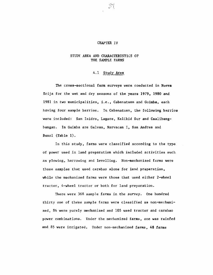
4.1 Study Area

The c r o s s - s e c t i o n a l farm surveys were conducted i n Nueva

E c i j a f o r t h e w e t and d ry seasons of t h e y e a r s 1979, 1980 and

1981 i n two m u n i c i p a l i t i e s , i . e . , Cabanatuan and Guimba, each

having f o u r sample b a r r i o s . I n Cabanatuan, t h e fo l l owing b a r r i o s

were inc luded : San I s i d r o , Lagare , Ka l i k id Sur and Caalibang-

bangan. I n Guimba a r e Galvan, Narvacan I, San Andres and

Bun01 (Tab l e 1 ) . I n t h i s s t u d y , farms were c l a s s i f i e d accord ing t o t h e type

of power used i n land p r e p a r a t i o n which inc luded a c t i v i t i e s such

a s plowing, harrowing and l e v e l l i n g . Non-mechanized farms were

t hose samples t h a t used carabao a l o n e f o r l and p r e p a r a t i o n ,

wh i l e t h e mechanized farms were t hose t h a t used e i t h e r 2-wheel

t r a c t o r , 4-wheel t r a c t o r o r b o t h f o r l and p r e p a r a t i o n .

There were 368 sample farms i n t h e survey. One hundred

t h i r t y one of the-se sample farms were c l a s s i f i e d as non-mechani-

zed, 86 were pu re ly mechanized and 105 used t r a c t o r and carabao

power combinations. Under t h e mechanized farms, one w a s r a i n f e d

and 85 were i r r i g a t e d , Under non-mechanized fa rms , 48 farms

Table 1. Distribution of sample farms by municipality and barrio, Nueva Ecija, Philippines, 1979

MUNICIPALITY/BARRIO NUMBER OF SAMPLE HOUSEHOLDS

Cabanatuan

San Isidro

Lagare

Kalikid Sur

Caalibangbangan 7 6

Guimba

Galvan

Narvacan I

San Andres

Bun01

were irrigated and 83 were rainfed (Table 2). The remaining

46 farmer respondents were landless field workers.

4.2 Characteristics of Sample Fanns

The samples selected for inclusion in the present study

were those farms that were irrigated and users of modern rice

varieties. It was not possihle to pick samples from the rainfed

farms since none of the respondents used tractor(s) for land

preparation (Table 2). There were those that used tractor(.),

however, they are in combination with carabao power in preparing

the field.

Demographic characteristics of sample farms, i.e,, age,

number of years in school and experience in farming, as shown

in Table 3, did not differ much between farm types.

In terms of farm area (Table 41, 2-wheel tractor farms were

on the average, 1.22 times larger than carabao farms and 1.5

times larger than the 2-wheel(4-wheel-tractor combination farms.

Cropping intensity was lowest for the carabao farms. Both

mechanized farm types had cropping intensities of 1.5 higher than

the carabao farms.

Yield per hectare was more than 1.5 times higher in the

mechanized farms than the non-mechanized farms.

Pre-harvest labor excluding land preparation did not vary

much between the farm types. On the other hand, post-production

Table 2. Distribution of sample farms by type of power used in land preparation and Irrigation, Nueva Ecija, Philippines, Wet Season, 1979

POWER IRRIGATION

Gravity Deep well Rainfed Total

Carabao 11 3 7 83 131

2-wheel tractor 62 1 1 64

4-wheel tractor 2 - - 2

2-wheell4-wheel tractor combination 2 0 .- - 2 0

Total 146 52 124 322

Table 3 . Demographic c h a r a c t e r i s t i c of sample farms by t y p e of mechan iza t ion , Nueva E c i j a , P h i l i p p i n e s , Wet Season, 1979

2-WHEEL 2-4 WHEEL CHARACTERISTICS TRACTOR TRACTOR

FARMS FARMS FARMS

Number of households 46 6 2 2 0

Average age of t h e household head ( y e a r s ) 44 49 46

Average e d u c a t i o n of household head ( y e a r s ) 4 4 4

Average e x p e r i e n c e i n farming of household head ( y e a r s ) 19 22 18

Table 4. C h a r a c t e r i s t i c s of sample farms by type of me'chani- z a t i o n , Nueva E c i j a , P h i l i p p i n e s , Wet Season, 1979

--.-- -* - 2-WHEEL 2-4 WHEEL

OPERATION FARMS FARMS TRACTOR TRACTOR FARMS

Area ( h e c t a r e s ) 1.95 2.39 1.59

Produc t ion (ki lograms) 5089.50 9591.93 7710.85

Y i e l d p e r h e c t a r e (kgs . ) 2610.00 4013.36 3702.54

P r i c e of paddy (f /kg. ) 1.06 1.17 1.05

T o t a l p re -harves t l a b o r (m-hrs /ha. ) 247.02 223.28 259.61

T o t a l post -product ion l a b o r (m-hrs /ha . ) 244.41 207.34 222.58

T o t a l l and p r e p a r a t i o n hours (man-machine o r man-animal h o u r s l h e c t a r e ) 96.79 29.52 28.10

Level of f e r t i l i z e r (kg.N/ha)

Value of c r o p p r o t e c t i o n ( f /ha) 96.69 186.44 145.52

Loan f o r s e a s o n a l farm expense p e r h e c t a r e 1023.44 1215.35 902.77

Long term l o a n f o r a g r i c u l t u r a l investment p e r h e c t a r e 1954.87 2484.56 3081.76

Cropping i n t e n s i t y * 1.36 1.92 1.97

* g r o s s cropped a r e a i n a g iven c r o p y e a r x 100 Cropping i n t e n s i t y = Operated a r e a p e r c r o p

- computed f o r wet and d r y season d a t a

l a b o r which i nc ludes h a r v e s t i n g , t h r e s h i n g and winnowing, was

h i g h e s t i n t h e carabao farms fol lowed by 2-wheel14-wheel-

t r a c t o r combination and 2 - h e e l t r a c t o r farms. This h ighe r

post-product ion l a b o r of t h e carabao farms over t h e t r a c t o r

farms was due t o t h e wide u se of t h r e s h e r s by t h e t r a c t o r farms

i n s t e a d of manually threshing t h e h a r v e s t .

Land p r e p a r a t i o n hours , however, showed a s h a r p drop from

t h e average 96.79 man-animal hours of t h e ca rabao farms t o

29.52 and 28.10 man-machine hours of t h e mechanized farms.

F e r t i l i z e r u se and c rop p r o t e c t i o n , i . e . , u s e of i n s e c t -

i c i d e s , weedicides and r o d e n t i c i d e s were c o n s i s t e n t l y h i g h e r

on t h e mechanized than t h e non-mechanized farms.

Short-term loan f o r s ea sona l farm expense p e r h e c t a r e

was h ighes t i n t h e 2-wheel t r a c t o r farms fol lowed by ca rabao

and 2-wheell4-wheel t r a c t o r combination farms. Long-term loans ,

however, used f o r a g r i c u l t u r a l inves tment , i . e . , purchase of

farm machines, carabao and i r r i g a t i o n pumps, was h ighe r on bo th

mechanized than t h e non-mechanized farms.

CHAPTER V

RESULTS AND DISCUSSION

This Chapter presents the major results of the study. De-

composition Models I and I1 were employed to evaluate whether

mechanization increases output or not. The observed output

differences between farms "with and without" mechanization was

disaggregated into the factors that brought about such

differences.

5.1 Results of the Arithmetic Decomposition Scheme

Production variables of mechanized and non-mechanized farms

were investigated and tested for differences using the Kruskal-

Wallis one-way analysis of variance by ranks. Table 5 shows

that area for the dry season, average area between wet and dry

seasons, yield for the wet season, average yield for the wet

and dry seasons, price for the wet season, average price,

fertilizer use, level of crop protection and land preparation

hours were all significantly different between 2-wheel tractor

and carabao farms. In the case of the 2-wheell4-wheel tractor

combination versus carabao farms, the following variables,

namely, area for dry season, yield for wet season, average

yield, price for dry season, fertilizer use, level of crop

protection, labor hours and land preparation hours showed

� able 5. T e s t f o r d i f f e r e n c e s of v a r i a b l e s between t r a c t o r and ca rabao farms u s i n g t h e Kruskal-Wal l is one-way a n a l y s i s of v a r i a n c e by ranks

VALUE OF H***

VARIABLES 2-wheel 2-wheel/4-wheel t r a c t o r farms v s . t r a c t o r farms v s . ca rabao farms ca rabao farms

Area (wet season)

Area (d ry season)

Average a r e a

Yie ld (wet season)

Yie ld (d ry season)

Average y i e l d

P r i c e (wet season)

P r i c e (dry season)

Average p r i c e

F e r t i l i z e r u s e

Level of c rop p r o t e c t i o n

Labor hours

Land p r e p a r a t i o n h o u r s

n. s . - not s i g n i f i c a n t

* - s i g n i f i c a n t a t 5% l e v e l

** - s i g n i f i c a n t a t 1% l e v e l

*** - s e e Appendix I1

signicant statistical differences. These results provided a

good reason to decompose the possible production effects of

mechanization.

Decomposition analysis was carried out for 2-wheel tractor

and 2-wheel/4-wheel-tractor combination against carabao farms.

The results of the analyses are presented in Tables 7 to 14.

Decomposition of output differences between farms using

2-wheel tractor and carabao farms employing Binswanger's made1

without interaction terms (Table 7) showed that the component

which contributed the largest percentage to the output differ-

ence is the cropping intensity effect (47.59%) followed by the

overall yield effect (39.23%) and area effect (13.18%). Break-

ing out a price effect from the overall yield effect (Table 8)

showed that 7.83% of the difference in output is due to the

difference in prices received by the two farm types. This

left a pure yield effect of 31.40%.

Using the version with interaction terms showed the same

overall yield effect (39.23%). Cropping intensity effect

went down to 26.01% (Table 9). Breaking out a price effect

resulted in a percentage contribution of price of 4.96% and

pure yield effect of 31.40% (Table 10). The area effect was

hardly changed registering 11.22%. This is quite expected

since the decision of farmers to increase area devoted to

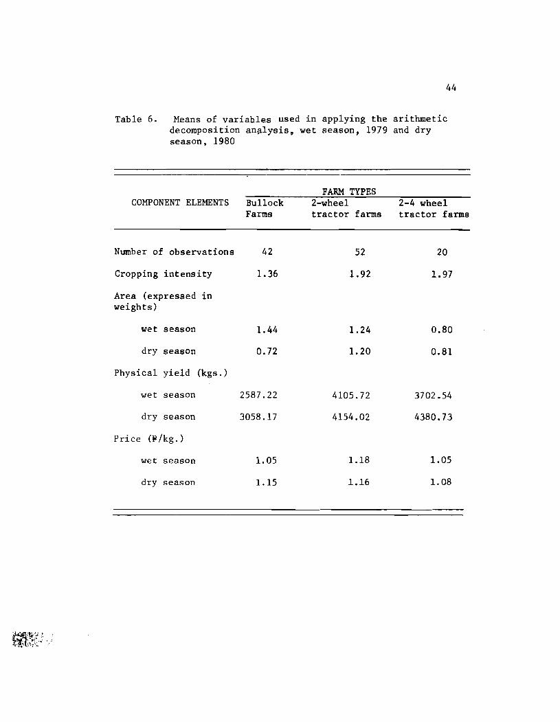
Table 6. Means of v a r i a b l e s used i n a p p l y i n g t h e a r i t h m e t i c decomposi t ion a n a l y s i s , wet s e a s o n , 1979 and d r y s e a s o n , 1980

FARM TYPES COMPONENT ELEMENTS Bul lock 2-wheel 2-4 wheel

Farms t r a c t o r farms t r a c t o r f a rms

Number of o b s e r v a t i o n s 4 2 52 20

Cropping i n t e n s i t y 1.36 1 .92 1.97

Area (expressed i n w e i g h t s )

wet season

d ry s e a s o n

P h y s i c a l y i e l d (kgs . )

wet season

d r y season

P r i c e ( ~ I k g . )

wet season

dry season

Table 7. Decomposit ion a n a l y s i s (wi thou t i n t e r a c t i o n t e rms) of o u t p u t d i f f e r e n c e s between 2-wheel t r a c t o r and c a r a b a o fa rms

EFFECTS ABSOLUTE PERCENTAGE CHANGE SHARE

Sources of o u t p u t d i f f e r e n c e s

o v e r a l l y i e l d e f f e c t 5442.50 39.23

a r e a e f f e c t 1827.85 13.18

c ropp ing i n t e n s i t y e f f e c t 6602.34 47.59

T o t a l 13872.70 100.00

Table 8. Decomposition a n a l y s i s (wi thou t i n t e r a c t i o n t e rms) of o u t p u t d i f f e r e n c e s between 2-wheel t r a c t o r and ca rabao farms w i t h p r i c e v a r i a b l e



p r i c e e f f e c t 1085.96 7 .83

pure y i e l d e f f e c t 4356.54 31.40

a r e a e f f e c t 1827.85 13.18

c ropp ing i n t e n s i t y e f f e c t 6602.34 47.59

Total. 13872.70 100.00

Table 9 . Decomposition a n a l y s i s (with i n t e r a c t i o n terms) of output d i f f e r ences between 2-wheel t r a c t o r and carabao farms


Sources of output d i f f e r e n c e s

A. Ind iv idua l e f f e c t s

o v e r a l l y i e l d e f f e c t 5442.50 39.23

Area e f f e c t 1556.92 11.22

Cropping i n t e n s i t y 3608.66 26.01

B. F i r s t -o rde r i n t e r a c t i o n e f f e c t s

y i e l d and a rea 270.93 1.95

cropping i n t e n s i t y and a rea 641.08 4.62

cropping i n t e n s i t y and y i e l d 2241.03 16.15

C. Second-order i n t e r a c t i o n e f f e c t

cropping i n t e n s i t y , a r e a and y i e l d 111.56 0.82

To ta l 13872.70 100.00

Table 10. Decomposition a n a l y s i s (wi th i n t e r a c t i o n t e rms) of o u t p u t d i f f e r e n c e s between 2-wheel t r a c t o r and c a r a b a o farms w i t h p r i E e v a r i a b l e

EFFECT ABSOLUTE PERCENTAGE CHANGE SHARE


A. I n d i v i d u a l e f f e c t s

p u r e y i e l d e f f e c t

a r e a e f f e c t

c ropp ing i n t e n s i t y e f f e c t

p r i c e e f f e c t

B. F i r s t - o r d e r i n t e r a c t i o n - e f f e c t s

y i e l d and p r i c e

a r e a and p r i c e

a r e a and y i e l d

c ropp ing i n t e n s i t y and y i e l d

c ropp ing i n t e n s i t y and p r i c e

c ropp ing i n t e n s i t y and a r e a

C. Second-order i n t e r a c t i o n e f f e c t s

c ropp ing i n t e n s i t y , p r i c e and a r e a

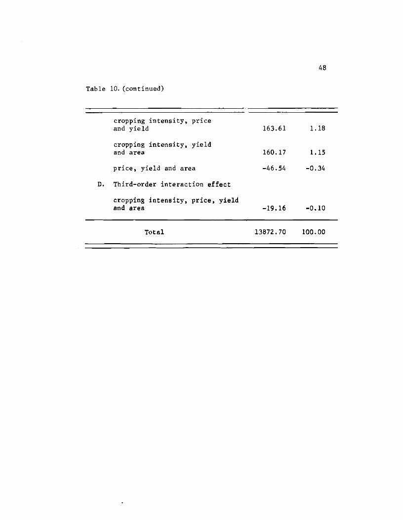
Table 10. (continued)

cropping i n t e n s i t y , p r i c e and y i e l d

cropping i n t e n s i t y , y i e l d and area

p r i c e , y i e l d and area -46.54 -0.34

D . Third-order i n t e r a c t i o n e f f e c t

cropping i n t e n s i t y , p r i c e , y i e l d and area

Tota l 13872.70 100.00

rice production is not likely to be influenced by 'factors of

productivity like yield and cropping intensity. It is

controlled by other factors that are not incorporated in the

model, such as increases in demand, government investment in

land reclamation, irrigation, credit and extension services,

or private investment due to relative profitability as a

result of better returns even at increased cost of land rent

and acquisition.

Since the area effect is the same for both models, i. e.,

with and without interaction terms, then the interaction

effects could only be expected to come out from the simulta-

neous change in cropping intensity and yield.

From Table 9, the largest interaction effect resulted from

cropping intensity and yield (16.152). Interaction effects of

area with yield and with cropping intensity were relatively

small, 1.95% and 4.62% respectively.

Breaking out interaction effects of price with yield and

cropping intensity showed quantitatively small percentage

contribution (1.86% and 2.04% respectively). The interaction

effect of cropping intensity with physical yield decreased

to 12.93%, however, it is still the largest percentage contri-

bution in the set of first order interaction effects, The

second-order and third order interation effects of the

component elements showed very little percentage contribution

(Table 10 ) .

I n t h e c a s e of t h e decomposit ion of ou tpu t between 2-wheel/

4 -whee l - t rac to r combination and carabao farms, t h e e f f e c t s of

t h e component e lements showed e x a c t l y t h e same p a t t e r n a s t h e

2-wheel t r a c t o r ve r su s carabao farms. Using t h e model with-

ou t i n t e r a c t i o n terms (Table 11) showed t h a t c ropping

i n t e n s i t y e f f e c t gave t h e h i g h e s t pe rcen tage c o n t r i b u t i o n

(86.95%) fol lowed by t h e o v e r a l l y i e l d e f f e c t (71.59%) and

a r e a e f f e c t (-58.54%). Breaking o u t a p r i c e e f f e c t (Table

12) r e s u l t e d t o 6.16%. The n e g a t i v e s i g n sugges t s t h a t t h e

average va lue of a component f o r 2-wheel/4-wheel-tractor

combination farms i s lower than t h e average v a l u e f o r ca rabao

farms.

Employing t h e model w i t h i n t e r a c t i o n terms gave t h e same

o v e r a l l y i e l d e f f e c t of 71.59% (Table 13 ) . Cropping i n t e n s i t y

and a r e a e f f e c t s went down s l i g h t l y t o 81.07% and -40.40%

r e s p e c t i v e l y . With r e s p e c t t o p r i c e e f f e c t , i t decreased t o

-4.31% (Table 14) .

Among t h e f i r s t - o r d e r i n t e r a c t i o n e f f e c t s , t h e i n t e r a c t i o n

between y i e l d and cropping i n t e n s i t y r e g i s t e r e d t h e h i g h e s t

pe rcen tage c o n t r i b u t i o n bo th i n t h e model w i thou t and w i t h

p r i c e v a r i a b l e (32.22% and 34.99% r e s p e c t i v e l y ) . The second-

o rde r and t h i rd -o rde r i n t e r a c t i o n e f f e c t s gave very low

percen tage c o n t r i b u t i o n s .

Table 11. Decomposition analysis (without interaction terms) of output difference between 2-~heel/4-~h~el-tracto~ combination and carabao farms


Sources of output differences

yield effect 3482.50 71.59

area effect -2847.48 -58.54

cropping intensity effect 4229.51 86.95

Tot a1 4864.53 100.00

Table 12. Decomposition analysis (without interaction terms) of output differences between 2-wheell4-wheel-tractor combination and carabao farms with price variable


Sources of output differences

yield effect 3782.76 77.76

area effect -2847.47 -58.54

cropping intensity effect 4229.51 86.94

price effect -300.27 -6.16

Tot a1 4864.53 100.00

Table 13. Decomposition a n a l y s i s (wi th i n t e r a c t i o n t e rms) of ou tpu t d i f f e r e n c e s between 2-wheel/4-wheel-tractor combination and ca rabao farms


Sources o f o u t p u t d i f f e r e n c e s

A . I n d i v i d u a l e f f e c t s

y i e l d e f f e c t

a r e a e f f e c t


B. F i r s t - o r d e r i n t e r a c t i o n e f f e c t s

y i e l d and a r e a

y i e l d and cropping i n t e n s i t y

a r e a and c ropp ing i n t e n s i t y

C. Second-order i n t e r a c t i o n e f f e c t

c ropp ing i n t e n s i t y , a r e a and y i e l d -396.96 -8.17

T o t a l 4864.53 100.00

Table 1 4 , Decomposition a n a l y s i s (wi th i n t e r a c t i o n t e r n s ) o f o u t p u t d i f f erencea between 2-wheel/4-wheel-trac t o r combination and ca rabao farms w i t h p r i c e v a r i a b l e



A. I n d i v i d u a l e f f e c t s

y i e l d e f f e c t

a r e a e f f e c t


p r i c e e f f e c t

B. F i r s t - o r d e r i n t e r a c t i o n e f f e c t s

y i e l d and p r i c e

a r e a and p r i c e

a r e a and y i e l d

c ropp ing i n t e n s i t y and a r e a

c ropp ing i n t e n s i t y and y i e l d

c ropp ing i n t e n s i t y and p r i c e

C. Second-order i n t e r a c t i o n e f f e c t s

c ropp ing i n t e n s i t y , p r i c e and a r e a

c ropp ing i n t e n s i t y , p r i c e and y i e l d

Table 14 (continued)

cropping i n t e n s i t y , y i e l d and area -381.00 -7.83

p r i c e , y i e l d and area -10.70 -0.22

D . Third-order i n t e r a c t i o n e f f e c t

y i e l d , p r i c e , area and cropping i n t e n s i t y

Total 4864.53 100.00

These decomposition analyses showed that the most important

factors explaining output differences between mechanized and

non-mechanized farms were cropping intesity and yield. The

two other factors, area and price bear little significance in

bringing about productivity differences. These results,

therefore, lead to the identification of variables that are

possibly affected by mechanization.

Cropping intensity, as the major component that explained

differences in output between mechanized and non-mechanized

farms was further investigated. Table 15 summarizes the crop-

ping intensities of the sample farme by type of irrigation and

eource of power for land preparation. It ehowe that farme

using dam or gravity irrigation have consistently higher

cropping intensities than rainfed or deep wells. With respect

to each of the irrigation categories, farms were grouped

according to whether they are tractor farms, carabao farms or

combination of carabao and tractor farms. Cropping intensities

of each farm type under each irrigation category were compared.

The comparison showed that tractor farms and tractor/carabao

combination farms have higher cropping intensities than the

carabao farms by 17.4% and 19.9% respectively.

Under deep wee1 irrigation, the cropping intensity of the

carabao/tractor combination was higher than carabao farms by

8.4%. For rainfed farms, cropping intensities of the carabao

Tab l e 1 5 . Cropping intensity of sample farms by type of power ueed i n land preparabion and irr igat ion, wet seaeon, 1979 and dry eeason, 1988

POWER IRRIGATION Gravity Deep well Rainfed

Carabao farms 161% 119% 103%

Trac to r farms 189% - - Tractor-Carabao combination

- no sample

farms and tractor combination farms showed no difference.

This is of course expected since rainfed farms are constrained

by water availability in the dry season.

These results showed that irrigation was a major factor

that affect cropping intensity but some variation did occur

when type of irrigation was held constant for the different

farm types by degree of mechanization.

Table 16 ehows a much disaggregated sample farms by

degree of mechanization. Again, under gravity irrigation,

tractor farms and tractorlcarabao combination farms have

consistently higher cropping intensities than the carabao

farms. For deep well and rainfed farms, little difference was

observed in the cropping intensities of all farm groups by

type of mechanization.

These results showed that under no water-constraint condi-

tion, farmers still vary in their decisions whether to plant

during the second season. In this analysis, mechanization

appears to be a factor that potentially increases cropping

intensity. However, full credit could not be placed solely on

mechanization for the apparent differences in cropping intensi-

ties. One striking confounding factor in this respect is that

tractor farms are often either better endowed with capital or

have better access to credit markets which enable the farmers

Table 16. Cropping intensity of sample farms by type of power used in land preparation and irrigation, wet season 1979 and dry season 1980

POWER IRRIGATION Gravity Deep well Rainfed

Carabao farms 161% 119% 103%

2-wheel tractor farms 192% * 1

4-3heel tractor farms * * - - 2-wheell4-wheel tractor combination 197% - - 2-wheellcarabao combination 195% * 100%

4-wheellcarabao combination * 115% 101%

2-wheelj4-wheellcarabao combination 175% * * *.

- no sample

* only one sample

** only two samples

59

to buy the necessary inputs hence afford a second crop (refer

to Table 3). This confounding factor, of course, magnifies

the cropping intensity effect of mechanization.

5.2 Results of the Decomposition Scheme Using the Production

Function Framework

Since the second largest component explaining differences

in output between mechanized and non-mechanized farms is yield,

another decomposition technique using the Cobb-Doubles product-

ion function was employed. This scheme disaggregated differences

in per hectare paddy output into components brought about by

technical change (neutral and non-neutral technological change)

and changes in the levels of inputs used.

Cobb-Douglas production functions were fitted for the

mechanized and non-mechanized farms. The generated coefficients

of the production functions for the three farm types are

presented in the following Tables 17, 18 and 19.

The coefficients of the per hectare production functions

for both mechanized and the non-mechanized farms showed consis-

tent results with respect to expected signs, though not all

variables turned out to be significant. When variable area was

incorporated in the model, some of the generated coefficients

gave negative signs(Tab1e 18 and 19). This is due to the high

multicollinearity of area with the other four variables.

Table 1 7 , Estimated coefficients of the Cobb-Douglas production function for the 2-wheel tractor farms

INDEPENDENT VARIABLES

DEPENDENT VARIABLES Total out~ut Yield /hectare

Intercept

Power

Fertilizer use

Labor

Crop protection

Area

Figure in parentheses are probabilities of J T J > 't ' statistic

* significant at 5% level

** significant at 1% level

Table 18. Estimated c o e f f i c i ~ t s of t h e Cobb-Douglas production func t ion f o r t h e c :abao farms

INDEPENDENT DEPENDENT VARIABLES VARIABLES To ta l output Yield/Hectare

I n t e r c e p t 7.37** 6.4**

Power

F e r t i l i z e r use

Labor -0 .05 0.005 (0 .6076 ) ( 0 .9622 )

Crop p r o t e c t i o n 0.38** 0.34**

Area 0.62** -

Figures i n paren theses a 2 p r o b a b i l j t i e s of I T 1 > ' t ' s t a t i s t i c .

* s i g n i f i c a n t a t 5% l e v c l .

** s i g n i f i c a n t a t 1% l e v e l .

Table 19. Es t ima ted c o e f f i c i ? n t s of t h e Cobb-Douglas p r o d u c t i o n f u n c t i o n f o r t h e 2-wheel/4-wheel t r a c t o r combinat ion farms

DEPENDENT VARIABLES INDEPENDENT VARIABLES T o t a l o u t p u t Y i e l d I H e c t a r e

I n t e r c e p t 9.27**

Power

F e r t i l i z e r u s e 0 .09 (0.8489)

Labor

Crop p r o t e c t i o n -0.18 (0.6207)

Area 0.38*

F i g u r e s i n p a r e n t h e s e s a r e p r o b a b i l i t i e s of ( T ( >' t ' s t a t i s t i c

* s i g n i f i c a n t a t 5% l e v e l

** s i g n i f i c a n t a t 1% l e v e l

Among t h e indenpendent v a r i a b l e s f o r mechanized fa rms ,

f e r t i l i z e r u s e , c a p i t a l s e r v i c e s and c r o p p r o t e c t i o n showed

s i g n i f i c a n t c o e f f i c i e n t s w h i l e i n t h e c a s e of t h e non-mechanized

farms, o n l y c r o p p r o t e c t i o n tu rned o u t t o be s i g n i f i c a n t

(Tab le 17 , 18 and 19) .

The p r o d u c t i o n e l a s t i c i t y f o r l a b o r , a l t h o u g h non-

s i g n i f i c a n t i n a l l t h r e e p r o d u c t i o n f u n c t i o n s , was h i g h e r i n

t h e mechanized farms t h a n t h e non-mechanized fa rms .

F e r t i l i z e r u s e had t h e h i g h e s t p r o d u c t i o n e l a s t i c i t y f o r

t h e 2-wheel t r a c t o r farms. Non-mechanized farms had t h e , lowes t

p r o d u c t i o n e l a s t i c i t y f o r f e r t i l i z e r u s e b u t i t had t h e h i g h e s t

f o r c r o p p r o t e c t i o n .

I n t h e c a s e of power v a r i a b l e , mechanized farms showed

h i g h e r p r o d u c t i o n e l a s t i c i t i e s t h a n t h e non-mechanized farms.

Area showed a p o s i t i v e p r o d u c t i o n e l a s t i c i t y f o r a l l t h r e e

farm t y p e s . T h i s is q u i t e c o n t r a r y t o t h e common i n v e r s e

r e l a t i o n s h i p of farm s i z e and p r o d u c t i v i t y . However, s i n c e t h e

s i z e of t h e farms used i n t h i s s t u d y were a l l s m a l l , r a n g i n g

from 0.5 t o 4 h e c t a r e s , t h e f i t t e d p r o d u c t i o n f u n c t i o n s may n o t

have c a p t u r e d t h e s c a l e e f f e c t .

The s t r u c t u r a l d i f f e r e n c e of t h e p r o d u c t i o n f u n c t i o n s

d e r i v e d from t h e 2-wheel t r a c t o r , 2-wheel /4-wheel- t rac tor

combinat ion and ca rabao farms were t e s t e d d u r i n g Chow's t e s t

(Appendix I V ) . The t e s t r e v e a l e d s i g n i f i c a n t d i f f e r e n c e s

between t h e 2-wheel t r a c t o r and ca rabao fa rms , b u t n o t

between t h e 2-wheel l4-wheel- t ractor combinat ion and ca rabao

farms. T h i s cou ld b e due t o t h e v e r y l i m i t e d sample s i z e

used i n f i t t i n g t h e p roduc t ion f u n c t i o n f o r t h e 2-wheell4-wheel

- t r a c t o r combination such t h a t t h e t r u e p r o d u c t i o n r e l a t i o n s

of i n p u t s t o o u t p u t s was n o t c a p t u r e d .

The s t r u c t u r a l d i f f e r e n c e between t h e two p r o d u c t i o n

f u n c t i o n s , i . e . , p r o d u c t i o n f u n c t i o n s f o r t h e 2-wheel t r a c t o r

farms and carabao farms was f u r t h e r t e s t e d u s i n g t h e dummy

101 v a r i a b l e approach - t o s e a r c h f o r t h e source of t h e s t r u c t u r a l

d i f f e r e n c e . Was i t due t o s h i f t i n t h e i n t e r c e p t term o r t o

t h e s h i f t i n t h e s l o p e c o e f f i c i e n t s , o r b o t h ? The dummy

v a r i a b l e t e s t showed t h a t t h e r e i s no s i g n i f i c a n t d i f f e r e n c e

between t h e two i n t e r c e p t terms. The only v a r i a b l e s t h a t showed

s i g n i f i c a n t s l o p e dummies were f e r t i l i z e r and c rop ~ r o t e c t i ' o n

(Table 20) . T h i s means t h a t t h e on ly s o u r c e of s t r u c t u r a l

d i f f e r e n c e between t h e 2-wheel t r a c t o r farms and ca rabao

fa3?ms were t h e shi f t s in the s l o p e c o e f f i c i e n t s of t h e s e

v a r i a b l e s .

With t h i s in fo rmat ion i n hand, a decomposi t ion scheme

employing t h e use of p roduc t ion f u n c t i o n framework was used.

101Oujarati, D. "Use of Dummy V a r i a b l e s i n T e s t i n g f o r E q u a l i t y Between S e t s of C o e f f i c i e n t s i n Two L i n e a r Regress ions : A Note" The American S t a t i s t i c i a n , Feb. 1970, pp. 50-52

Table 20. Test for structural differences in the production functions for 2-wheel tractor farms and farms using the dummy variable approach

INDEPENDENT VARIABLES DEPENDENT VARIABLE (Yield per hectare)

Intercept 5.39**

Intercept dummy

Power 0.20*

Fertilizer 0.44**

Labor

Crop protection

Slope dummy for power

Slope dummy for fertilizer -0.406**

Slope dummy for labor

Slope dummy for crop protection 0.33**

Figures in parentheses are probabilities of ( T I > 't' statistic.

* significant at 5% level. ** significant at 1% level.

Using Equat ion 7 of decomposit ion model I1 and u t i l i z i n g t h e

genera ted produc t ion c o e f f i c i e n t s (Table 17 and 18) and average

i npu t l e v e l s (Table 211, t o t a l changes i n p e r h e c t a r e y i e l d

d i f f e r e n c e s between 2-wheel t r a c t o r farms and ca rabaa farms

were decomposed i n t o f a c t o r s brought about by t e c h n i c a l change

and changes i n t h e l e v e l s of i n p u t s used. The r e s u l t s showed

t h a t t h e percen tage c o n t r i b u t i o n of t e c h n i c a l change was 48.71%

(Table 2 2 ) .

Technica l change a f f e c t s ou tpu t by s h i f t i n g e i t h e r t h e

i n t e r c e p t o r t h e s l o p e c o e f f i c i e n t s o r bo th . Disaggrega t ing

t e c h n i c a l change i n t o n e u t r a l and non-neu t ra l t e c h n i c a l e f f e c t s

i n d i c a t e s a -9.35% c o n t r i b u t i o n from t h e s h i f t i n t h e s c a l e

parameter and a 58.06% c o n t r i b u t i o n of t h e s h i f t i n t h e s l o p e

paramete rs .

The c o n t r i b u t i o n of t h e n e u t r a l t e c h n i c a l change was shown

t o be nega t i ve which means y i e l d is lower f o r t h e mechanized

farms when low l e v e l s of i n p u t s a r e used and h i g h e r y i e l d a r e

achieved on ly when i n p u t s a r e used i n s u f f i c i e n t amounts.

The c o n t r i b u t i o n of non-neutra l t e c h n i c a l change was e s t i -

mated t o be 58.06%. This means t h a t p roduc t ion on t h e mechanized

farms was h ighe r than mechanized farms because of t h e d i f f e r e n c e s

i n t h e a l l o c a t i o n of r e sou rce s t o t he d i f f e r e n t t ypes of i n p u t s

used. Non-neutral t e c h n i c a l change was shown t o be p o s i t i v e ,

.e 21. Means of variables used in applying the decomposition analysis using the production function framework, wet season, 1979

FARM TYPES

VARIABLE Carabao 2-wheel farms tractor farms

Number of observations 46 6 2

Yield (kglha) 2610.00 4013.36

Area (ha) 1.95 2.39

Labor (m-hrs) 247.02 223.28

power (m-animallmachine hrslha) 96.79

Fertilizer (kg ha) 40.13 57.98

Crop protection @/ha) 96.69 186.44

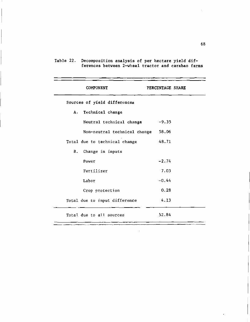
Table 22. Decomposition a n a l y s i s of per h e c t a r e y i e l d d i f - fe rences between 2-wheel t r a c t o r and carabao farms

COMPONENT PERCENTAGE SHARE

Sources of y i e l d d i f f e r ences

A . Technical change

Neutral t echn ica l change -9.35

Non-neutral t e c h n i c a l change 58.06

To ta l due t o t e c h n i c a l change 48.71

B. Change i n i npu t s

Power -2.74

F e r t i l i z e r 7.03

Labor -0.44

Crop p ro t ec t ion 0.28

Tota l due t o input d i f f e r e n c e 4.13

To ta l due t o a l l sources 52.84

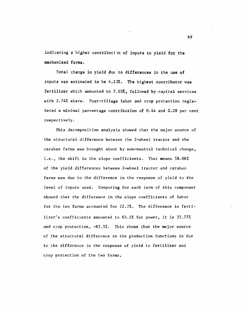
indicating a higher contributj~n of inputs to yield for the

mechanized farms.

Total change in yield duc to differences in the use of

inputs was estimated to be 4,13%. The highest contributor was

fertilizer which amounted to 7.032, followed by capital services

with 2.74% share. Post-tillage labor and crop protection regis-

tered a minimal percentage contribution of 0.44 and 0.28 per cent

respectively.

This decomposition analysis showed that the major source of

the structural difference between the 2-wheel tractor and the

carabao farms was brought about by non-neutral technical change,

i.e., the shift in the slope coefficients. That means 58.06%

of the yield differences between 2-wheel tractor and carabao

farms was due to the difference in the response of yield to the

level of inputs used. Computing for each term of this component

showed that the difference in the slope coefficients of labor

for the two farms accounted for 22.7%. The difference in ferti-

lizer's coefficients amounted to 65.1% for power, it is 35.77%

and crop protection, -65.5%. This shows that the major source

of the structural difference in the production functions is due

to the difference in the response of yield to fertilizer and

crop protection of the two farms.

CHAPTER YI

SUMMARY AND CONCLUSION

The main objective of this study was a quantitative assess-

ment of the impact of mechanization on small-scale rice produc-

tion. It aimed to isolate the sources of output differences be-

tween mechanized and non-mechanized farms. To evaluate production

effects of mechanization, decompos2tion analyses were used.

The first model tried was an arithmetic decomposition scheme

which disaggregated the output differences between the mechanized

and non-mechanized farms into the following component elements:

a. pure yield component

b. price component

c. area component

d. cropping intensity component

e. interactions of these four components

The results of the analysis showed that the most important

factors accounting for output differences between the mechanized

and non-mechanized farms were cropping intensity and yield.

Mechanization may increase cropping intensity since it allows

for faster completion of land preparation hence reducing the turn-

around time between crops. The results of the arithmetic decom-

position analysis seemed to support this thesis. Further

i n v e s t i g a t i o n of t he cropping i n t e n s i t y e f f e c t of mechanziation

showed t h a t a l though i r r i g a t i o n played a major r o l e i n t h e

cropping i n t e n s i t y d i f f e r e n c e s of t h e sample farms, some v a r i -

a t i o n d id occur when type of i r r i g a t i o n was he ld cons tan t f o r each

of t h e d i f f e r e n t farm types c l a s s i f i e d by degree of mechanization.

However, s i n c e t h e farmer 's d e c i s i o n t o p l a n t a second crop i s

based not on ly on water a v a i l a b i l i t y bu t a l s o on l i q u i d i t y , mecha-

n i z a t i o n , t h e r e f o r e , could no t be he ld fu1l.y r e spons ib l e f o r t h e

apparent d i f f e r e n c e s i n cropping i n t e n s i t i e s on t h e sample farms.

Yie ld , on t he o t h e r hand, p resen ted a more complicated e f f e c t ,

s i n c e i t is a f f e c t e d by f a c t o r s no t p r e sen t i n t h e model. To inves-

t i g a t e f u r t h e r t h i s y i e l d e f f e c t of mechanization, another decom-

p o s i t i o n technique was employed, us ing a product ion func t ion frame-

work. The model decomposed t o t a l y i e l d d i f f e r e n c e s between mecha-

nized and non-mechanized farms i n t o :

a . t e c h n i c a l change component

b. changes i n input used component

The r e s u l t s of t h e a n a l y s i s showed t h a t t h e major source of

y i e l d d i f f e r e n c e between t h e 2-wheel t r a c t o r farms and t h e carabao

farms was brought aboct by noncneutral t e c h n i c a l change, i . e . ,

s h i f t s i n t h e s l o p e c o e f f i c i e n t s of t h e product ion func t ions , o r

a d i f f e r e n c e i n t h e a l l o c a t i o n of resources f o r t h e two farm types.

7 2

These r e s u l t s , taken t o g e t h e r , showed t h a t mechanization

does i n c r e a s e ou tpu t , a l though no t impressive, by i n c r e a s i n g

cropping i n t e n s i t y and y i e l d . Confounding f a c t o r s such a s i rr i-

ga t ion , a v a i l a b i l i t y of c a p i t a l f o r cash i n p u t s l i k e f e r t i l i z e r s

and crop p r o t e c t i o n ; access t o c r e d i t markets and he te rogene i ty

of managerial q u a l i t y among sample farms played an i m p l i c i t r o l e

t h a t exaggerated t h e y i e l d and cropping i n t e n s i t y e f f e c t s of

mechanization.

The problem of " t rade-of fs" between inc reas ing product i o n

and inc reas ing employment must be weighed, t h e r e f o r e , i n t h e

l i g h t of t h e s e informations and must be c a r e f u l l y considered i n

implementing t a x , t a r i f f and c r e d i t p o l i c i e s f o r farmmechanizat ion.

LITERATURE CITED

ABERCROMBIE , K. C. "~gricultural Mechanization and Employment in Developing Countries," Effects of Farm Mechanization and Employment, FAOIOECD, Rome, 1975, pp. 35-49.

MRAMOVITZ, M. "Resources and Output Trends in the United States Since 1870". American Economic Review, Vol. 46, May 1956, pp. 5-23.

ALMARIO, E. S. "A Historical Approach to Agricultural Mechani- zation in the Philippines". Paper presented at the work- shop on the Consequences of Small Rice Farm Mechanization, IRRI, 1979.

ANTIPORTA., D. B. and Deomampo, N.R., "Employment Impact of Mechanization of Rice Production Processes", SEARCA Pro- fessorial Chair Lecture, U. P. at Los Bafios, September 1979.

BINSWANGER, H. Economics of Tractors in South Asia, A , , Nee York and ICRISAT, Hyderabad, India, 1978.

BISALIAH, S. "Effects of Technological Change on Output, Employ- and Functional Income Distribution in Indian Agriculture, A Case Study of' the Punjab Wheat Economy". Ph. D. is- sertation, University of Minnesota, November 1975.

BISALIAH, S. "Decomposition Analysis of Output Change Under New Production Technology in Wheat Farming: Some Impli- cations to Returns to Investment in Research:. Indian Journal of Agricultural Economics, Vol. 32, No. 1, Jan- March, 1977.

BISALIAH, S. "Decomposition Analysis of Employment Change under New Production Technology in Punjab Agriculture'' Indian Journal of Agricultural Economics, Vol. 33, No. 2, April- June, 1978.

BRADY, Nyle C. The Nature and Properties of Soils, 8th edition MacMillan Publishing Co. Inc, New York, 1974, p. 538.

CHOW, G. C., "Tests of Equality Between Sets of Coefficients in Two Linear Regressions", Econometrica, Vol. 28, No.-3, July, 1960, pp. 591-605.

DUFF , B. "Output, Employment and Mechanization in the Philip- pine Agriculture", Effects of Farm Mechanization and Employment, FAOIOECD, Rome, 1975. pp. 111-152.

DUFF, 5. "Mechan ization and Use of Modern Rice Varieties", Economic consequences of the New Rice Technology", IRRI, Los Baiios, Philippines, 1978.

FOLLOSCO, C. "Farm Mechanization and Its Economic Impacts" Agricultural and Industrial Life. Vol. 28, September, 1966.

GUJARATI, D. "Use of Dummy Variables in Testing for Equality Between Sets of Coefficients in Two Linear Regressions: A Note" The American Statistician, February 1970, pp. 50.52.

INUKAI, I. "Farm Mechanization Output and Labor Input: A Case Study in Thailand" International Labour Review. CI, 5 (May 1970) pp. 453-473.

KENDRICK, D. A. Productivity Trends in the United States. Princeton: Princeton University Press, 1961.

KRISHNA, R. "Measurement of the Direct and Indirect Employ- ment Effects of Agricultural Growth w/ Technical Change" Employment in Developing Nations. Edited by Edgar 0. Edwards, Columbia University Press, 1974.

McMENNAMY, J. A. "Machinery Development Program at the Inter- national Rice Research Institute". Paper presented at the Meeting of the Indian Society of Agricultural Engineers, Hyderabad, India, January 1976.

MINHAS, B.S. and Vaidyanathan A. "Growth of Crop Output in India, 1951-1954 to 1958-1961". Journal of the Indian Society of Agricultural Statistics, Vol. 17, No. 2, 1965.

MISRA, V. N. "Growth of Crop Output in Gujarat: A Component Analysisu Anvesak, Vol. 1, No. 1, June, 1971.

MORAN,P. and Unson D. "Farm Survey and Recordkeeping Proce- dures for Consequences of Small Rice Farm Mechanization Project: Operation Handbook" IRRI/USAID, May 1980.

PATEL, N. T. "Farm Tractorization, Its Impact on Agricul- tural Inputs and Outputs", Economic Times, India, Octo- ber 20, 1980.

PIPUTSITEE, C. "An Economic Analysis of Manufacturing and Distribution Activities in the Farm Machinery Industry in the Philippines" M. A. thesis, UP, 1976.

RATHORE, M. S. "Factor Combination and Resource Use Efficiency on Small and Large Farms - A Comparative Study of Hill Agriculture and the SAT", Ph. D. Dissertation, Himachal Pradesh University, Simla, 1979.

SAGAR, V. "A Component Analysis of the Growth of Productivity and Product ion in Raj asthan: 1956-61 to 1969-74" Indian Journal of Agricultural Economics, Vol. 32, No. 1, January- March, 1977.

SANTOS , G. "Mechanization Farming in the Philippines". M. A. Thesis. University of Sto. Tomas, 1946.

SIEGEL, S. Nonparametric Statistics for the Behavioral Sciences, McGraw-Hill Kogakusha, Ltd. 1956.

SOLOW, R. M. "Technical Change and the Aggregate Production Function", Review of Economics and Statistics, Vol. 39', August 1957, pp. 312-320.

SONDHI, R. and Singh K. "Component Analysis of Foodgrain Economy of India", Journal of Social and Economic Studies, Vol. 3, No. 2, September, 1975.

TENNENT , R. M. Science Data Book, Longman Group.Ltd., London 1975.

TI-LAPA, G. B. "The Economics of Tractor Ownership and Use in Selected Districts of the Nepal Terai". M. S. Thesis, UPLB, 1979.

APPENDIX I-A

Identity I

Proof:

Q.E.D.

APPENDIX I - B

I d e n t i t y I1

P r o o f :

0 0 0 0 1 1 l A 1 p l X 1 - rAop0xo = z~lp!xl - CA.P .x. + CA;P:X: - T A ~ P ~ X ~ i i i i i i I I i 1 1 1

1 0 1 1 0 0 = T ( A ~ - A ~ ) P ~ x ~ + TA;(P:X~ - pixi)

1 1 0 0 0 1 = zhip ix i + ZA;(P:X: - pixi + P;X: - pixi)

1 1 0 1 0 1 0 0 1 0 = CAAiPiXi + l A i ( P i - Pi)Xi + l A . P . ( X i - Xi) 1 1

1 1 0 1 0 0 = l A A . P . X . + CAiAPiXi + ZAiPimi Q.E.D.

1 1 1

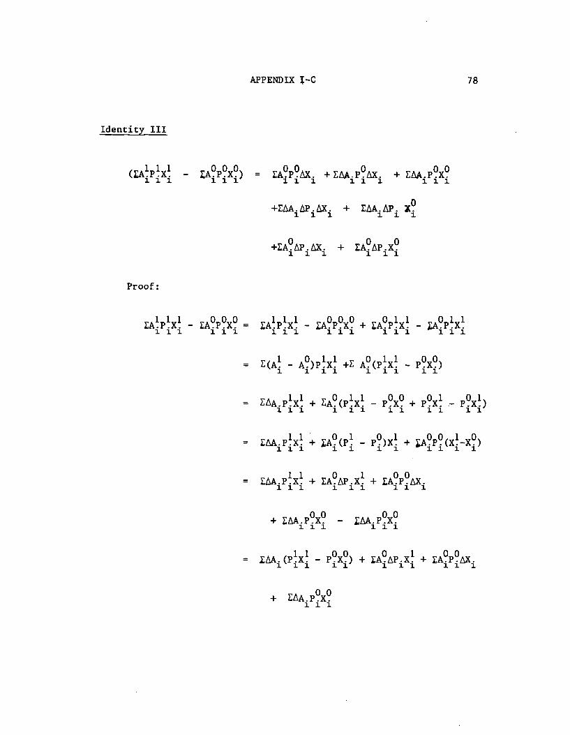
APPENDIX $-C

Iden t i ty I11

0 0 0 0 0 0 0 0 (u:P:x~ - ZA. P . X. ) = CAiPiAXi + ZAAiPiAXi + EAAiPiXi 1 1 1

P r o o f :

1 1 1 0 0 0 0 1 1 0 1 1 ZA;P:X; - CAI)P?XO 1 1 i = T A ~ P ~ X ~ - Z A ~ P ~ X ~ + T A ~ P ~ X ~ - EA.P.X

i 1 i

1 0 1 1 0 1 1 0 0 = z(Ai - Ai)PiXi +z Ai(PiXi - Pixi)

1 1 0 0 0 1 0 1 = L A A ~ P ~ x ~ + ZA~(P:X: - P .x. + P .x. - P .x.)

1 1 1 1 1 1

1 1 0 1 0 1 0 0 1 0 = m i p i x i + E A ~ ( P ~ - pi)xi + u i p i ( x i - x i )

1 1 0 1 0 0 = LAAiPiXi + CAihPiXi + CAiPiAXi

0 0 0 0 + GAAiPiXi - CAA.P.X. 1 1 1

1 1 0 0 0 1 0 0 = LAAi(PiXi - Pixi) + TAiAPiXi + CA.P.AX 1 1 i

0 0 + L A A ~ P ~ x ~

0 0 0 0 + ZAAiAPiXi + LAiAPiAXi + ZAiAPiXi ' Q.E.D.

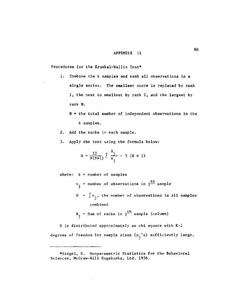
APPENDIX I1

Procedures f o r t h e Kruskal-Wallis Test*

1. Combine t h e k samples and rank a l l obse rva t i ons i n a

s i n g l e series. The smallest s c o r e i s r ep l aced by rank

1, t h e nex t t o s m a l l e s t by rank 2 , and t h e l a r g e s t by

rank N.

N = t h e t o t a l number of independent o b s e r v a t i o n s i n t h e

k samples.

2. Add t h e r anks i n e ach sample.

3. Apply t h e t e s t u s ing t h e formula below:

where: k = number of samples

t h n = number of obse rva t i ons i n j- sample j

N = I n j , t h e number of o b s e r v a t i o n s i n a l l samples

combined

t h R. = Sum of ranks i n j- sample (column) J

H i s d i s t r i b u t e d approximately a s c h i squa re w i th K-1

degrees of freedom f o r sample s i z e s ( n ' s ) s u f f i c i e n t l y l a r g e . j

*Siege l , S. Nonparametric S t a t i s t i c s f o r t h e Behaviora l Sc iences , McGraw-Hill Kogakusha, Ltd. 1956.

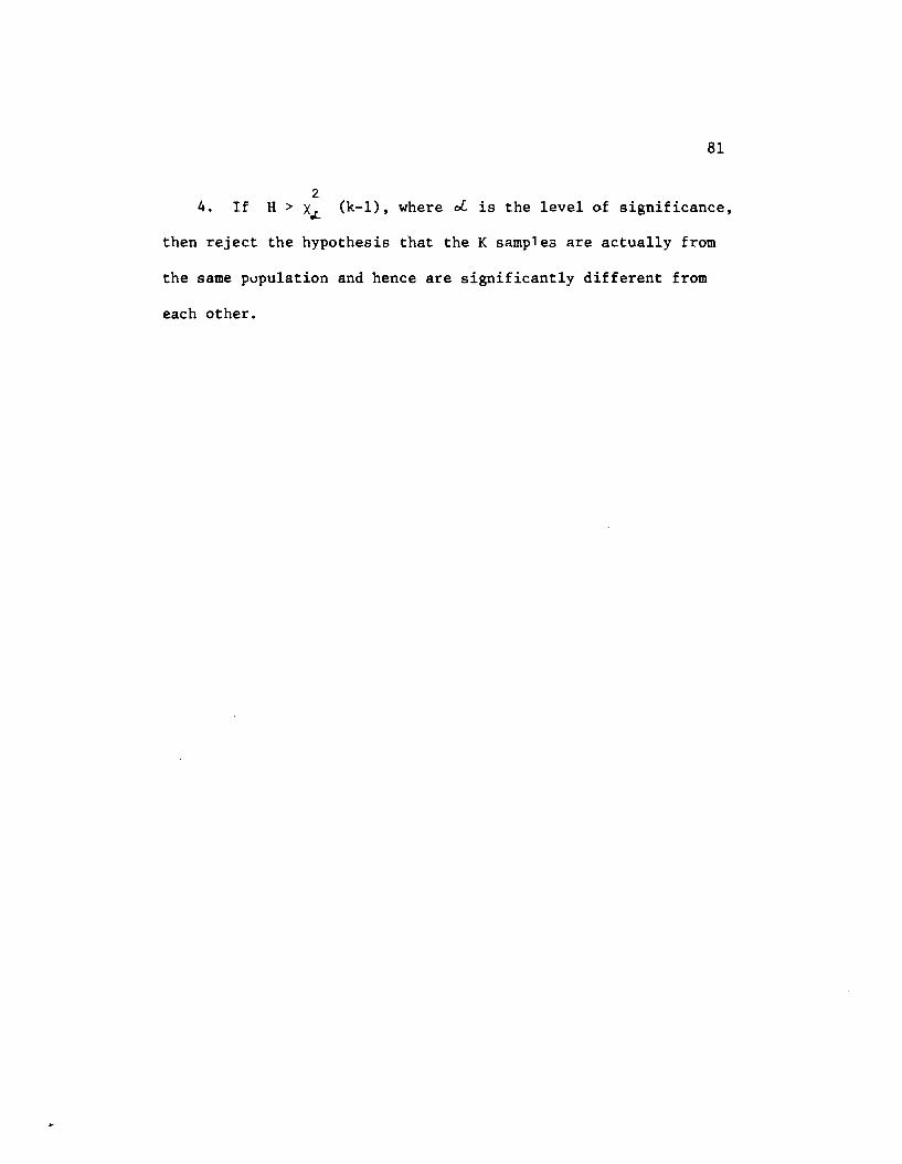
L

4. If H > xL (k-1), where d is the level of significance,

then reject the hypothesis that the K samples are actually from

the same population and hence are significantly different from

each other.

APPENDIX I11

log y1 = log ( l + X ) X i "I where :

X approximately measures the percentage change i n output i f the

higher order terms i n the Taylor's Expansion Ser ies are discarded s ince

the ir values w i l l be get t ing smaller and smaller for a l l ( X I < 1, i . e . ,

APPENDIX IV

1 / - 2/ Nitrogen content of organic- and commercial f e r t i l i z e r s :

comonly used conrmercial f e r t l i z e r s n i t rogen content

a . urea 457.

b. amnonium s u l f a t e 267.

c . amnonium ch lo r ide 2 57.

d. 16-20-00 167.

e . complete 147.

organic f e r t i l i z e r (farm manures)

a. da i ry c a t t l e

b. feeder c a t t l e

c . poul t ry

d. swine

e . horse

n i t rogen content ( l b . / ton)

10.0

11.9

29.9

12.9

14.9

1/ Brady N.C. The Nature and Proper t ies of S o i l s , 8 t h e d i t i o n - MacMillan Publishing Co. Inc . , New York: 1974, p.538

2/ Moran P. and Unson D . "Farm Survey and Recordkeeping Proce- - dures fo r Consequences of Small Rice Farm Mechanization P ro jec t : Operation Handbook" IRRI/uSAID, May 1980, p. 101.

APPENDIX V

Procedures for the Chow's Test*

1. Run separate linearized regressions of production

functions for mechanized and non-mechanized farms, i.e.

log Y = log A + Bllog Fm + B210g L + B310gKm + B410g Cm + Urn m m m

log Yb = log % + Z1log Fb + Z210g Lb + Z310g Kb+ Z410g Cb + U b

From these equations, obtain the error sum of squares SSE m

and SSE with degrees of freedom N -K and N -K respectively, b m b

where K is the number of parameters to be estimated. In this

example, K = 4. Add these two error sum of squares:

SSEs = (SSE, + SSEb) with d.f. (N + Nb - 2K) m

2 . Run another linearized production function combining

all.observations (N + N ) and get the error sum of squares m b

SSE with (Nm + Nb -K) degrees of freedom. t

3. Get the difference between SSE - SSE = SSEd t S

4. Apply the F-test: S S E ~ /K

F = SSE~/ (Nm + Nb -2K)

with degrees of freedom K and (N + Nb - 2K).

JIGujarati, D. "Use of Dummy Variables in Testing for Equality Between Sets of Coefficients in Two Linear Regressions: A Note" The American Statistician, February, 1970, pp. 50-52.

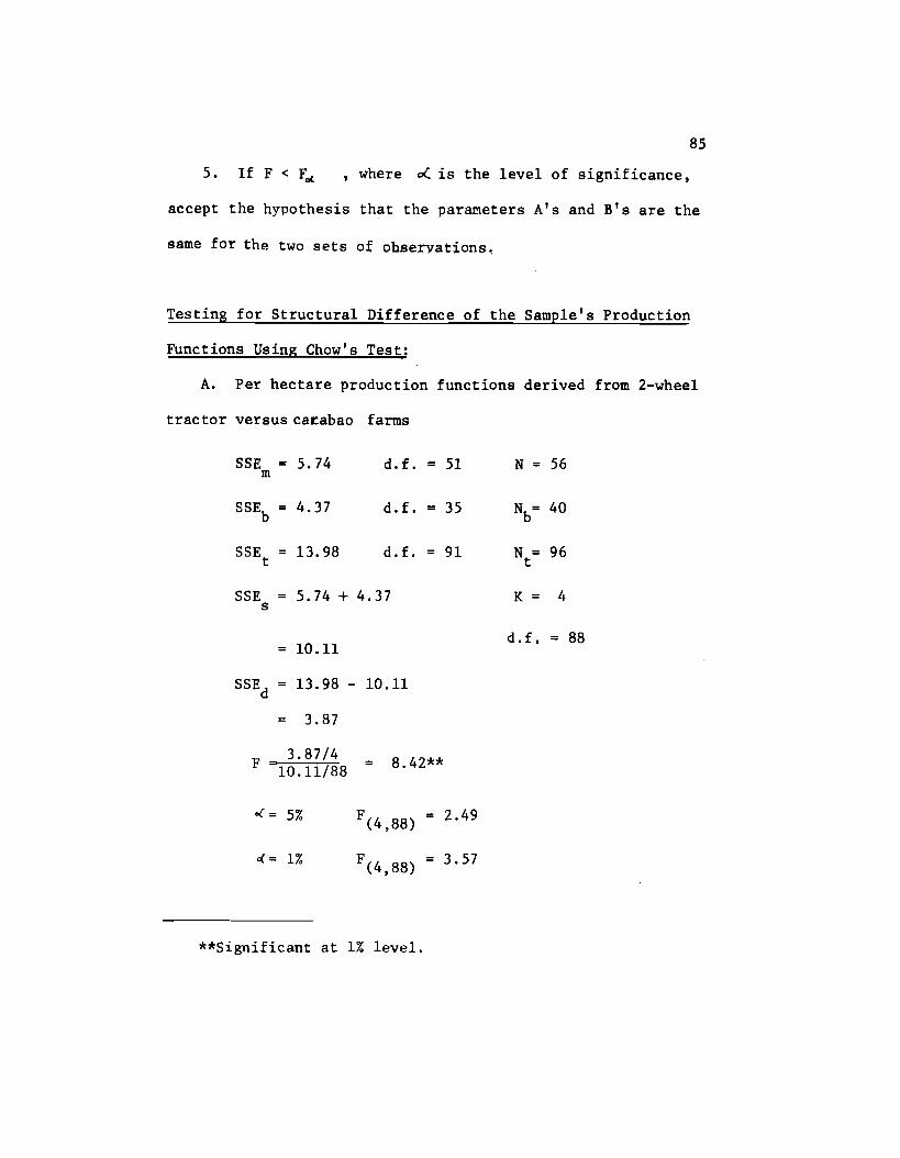
8 5

5. If F < F, , where &is the level of significance,

accept the hypothesis that the parameters A's and B's are the

same for the two sets of observations,

Testing for Structural Difference of the Sample's Production

Functions Usinn Chow's Test:

A. Per hectare production functions derived from 2-wheel

tractor versus carabao farms

SSE = 4.37 b d.f. = 35 Nb= 40

SSEt = 13.98 d.f. = 91 Nt= 96

SSE = 5.74 + 4.37 K = I+ S

SSE = 13.98 - 10.11 d

= 3.87

**Significant at 1% level.

B. P e r h e c t a r e p roduc t ion f u n c t i o n s d e r i v e d from 2-wheel/

4-wheel t r a c t o r combination v e r s u s ca rabao farms.

SSE = 7.49 m d . f . = 1 5 N = 20

m

SSEb = 4.37 d . f . = 35 N = 40 b

SSEt = 13.37 d . f . = 55 N t = 60

SSE = 7.49 + 4.37 s

n . s. - n o t s i g n i f i c a n t .

THE IMPACT OF FARM MECHANIZATION ON SMALL-SCALE RICE PRODUCTION

Documents

Transcript of THE IMPACT OF FARM MECHANIZATION ON SMALL-SCALE RICE PRODUCTION