The Effects Of Phosphate And Silicate Inhibitors On ...

University of Central Florida University of Central Florida

STARS STARS

Electronic Theses and Dissertations, 2004-2019

2008

The Effects Of Phosphate And Silicate Inhibitors On Surface The Effects Of Phosphate And Silicate Inhibitors On Surface

Roughness And Copper Release In Water Distribution Systems Roughness And Copper Release In Water Distribution Systems

David MacNevin University of Central Florida

Part of the Environmental Engineering Commons

Find similar works at: https://stars.library.ucf.edu/etd

University of Central Florida Libraries http://library.ucf.edu

This Doctoral Dissertation (Open Access) is brought to you for free and open access by STARS. It has been accepted

for inclusion in Electronic Theses and Dissertations, 2004-2019 by an authorized administrator of STARS. For more

information, please contact [email protected].

STARS Citation STARS Citation MacNevin, David, "The Effects Of Phosphate And Silicate Inhibitors On Surface Roughness And Copper Release In Water Distribution Systems" (2008). Electronic Theses and Dissertations, 2004-2019. 3607. https://stars.library.ucf.edu/etd/3607

https://stars.library.ucf.edu/



https://stars.library.ucf.edu/etd

http://network.bepress.com/hgg/discipline/254?utm_source=stars.library.ucf.edu%2Fetd%2F3607&utm_medium=PDF&utm_campaign=PDFCoverPages

https://stars.library.ucf.edu/etd

http://library.ucf.edu/

mailto:[email protected]

https://stars.library.ucf.edu/etd/3607?utm_source=stars.library.ucf.edu%2Fetd%2F3607&utm_medium=PDF&utm_campaign=PDFCoverPages



THE EFFECTS OF PHOSPHATE AND SILICATE INHIBITORS ON SURFACE ROUGHNESS AND COPPER RELEASE IN WATER DISTRIBUTION

SYSTEMS

by DAVID EARL MACNEVIN

B.S., University of Central Florida, 2005.

A dissertation submitted in partial fulfillment of the requirements for the degree of Doctor of Philosophy

in the Department of Civil and Environmental Engineering in the College of Engineering and Computer Science

at the University of Central Florida Orlando, Florida

Fall Term 2007

Major Professor: James S. Taylor

© 2007 David E. MacNevin

ii

ABSTRACT

The effects of corrosion inhibitors on water quality and the distribution system were

studied. This dissertation investigates the effect of inhibitors on iron surface roughness, copper

surface roughness, and copper release.

Corrosion inhibitors included blended poly/ortho phosphate, sodium orthophosphate, zinc

orthophosphate, and sodium silicate. These inhibitors were added to a blend of surface water,

groundwater, and desalinated brackish water.

Surface roughness of galvanized iron, unlined cast iron, lined cast iron, and polyvinyl

chloride was measured using pipe coupons exposed for three months. Roughness of each pipe

coupon was measured with an optical surface profiler before and after exposure to inhibitors. For

most materials, inhibitor did not have a significant effect on surface roughness; instead, the most

significant factor determining the final surface roughness was the initial surface roughness.

Coupons with low initial surface roughness tended to have an increase in surface roughness

during exposure, and vice versa, implying that surface roughness tended to regress towards an

average or equilibrium value. For unlined cast iron, increased alkalinity and increased

temperature tended to correspond with increases in surface roughness. Unlined cast iron coupons

receiving phosphate inhibitors were more likely to have a significant change in surface

roughness, suggesting that phosphate inhibitors affect stability of iron pipe scales.

Similar roughness data collected with new copper coupons showed that elevated

orthophosphate, alkalinity, and temperature were all factors associated with increased copper

surface roughness. The greatest increases in surface roughness were observed with copper

coupons receiving phosphate inhibitors. Smaller increases were observed with copper coupons

receiving silicate inhibitor or no inhibitor. With phosphate inhibitors, elevated temperature and

iii

alkalinity were associated with larger increases in surface roughness and blue-green copper (II)

scales.. Otherwise a compact, dull red copper (I) scale was observed. These data suggest that

phosphate inhibitor addition corresponds with changes in surface morphology, and surface

composition, including the oxidation state of copper solids.

The effects of corrosion inhibitors on copper surface chemistry and cuprosolvency were

investigated. Most copper scales had X-ray photoelectron spectroscopy binding energies

consistent with a mixture of Cu2O, CuO, Cu(OH)2, and other copper (II) salts. Orthophosphate

and silica were detected on copper surfaces exposed to each inhibitor.

All phosphate and silicate inhibitors reduced copper release relative to the no inhibitor

treatments, keeping total copper below the 1.3 mg/L MCLG for all water quality blends. All

three kinds of phosphate inhibitors, when added at 1 mg/L as P, corresponded with a 60%

reduction in copper release relative to the no inhibitor control. On average, this percent reduction

was consistent across varying water quality conditions in all four phases. Similarly when silicate

inhibitor was added at 6 mg/L as SiO2, this corresponded with a 25-40% reduction in copper

release relative to the no inhibitor control. Hence, on average, for the given inhibitors and doses,

phosphate inhibitors provided more predictable control of copper release across changing water

quality conditions. A plot of cupric ion concentration versus orthophosphate concentration

showed a decrease in copper release consistent with mechanistic control by either cupric

phosphate solubility or a diffusion limiting phosphate film.

Thermodynamic models were developed to identify feasible controlling solids. For the no

inhibitor treatment, Cu(OH)2 provided the closest prediction of copper release. With phosphate

inhibitors both Cu(OH)2 and Cu(PO4)·2H2O models provided plausible predictions. Similarly,

with silicate inhibitor, the Cu(OH)2 and CuSiO3·H2O models provided plausible predictions.

iv

ACKNOWLEDGMENTS

This dissertation would not have been possible without the contributions of my

coworkers in the Environmental Systems Engineering Institute. Staff members included Dr.

Charles Norris, Dr. John Dietz, and Maria Pia Real Robert. Fellow students who were essential

to this research include Abdul Alshehri, Tony Kwan, Philip Lintereur, Erica Stone, Raj Vaidya, ,

Bingjie Zhao, Avinash Shekhar, and Stephen Glatthorn. Raj provided many helpful comments

which have improved this manuscript. Committee members Dr. C. Clausen, Dr. S.J. Duranceau,

Dr. L. An, and Dr. A.A Randall, provided helpful technical feedback and guidance. I would

especially like to acknowledge the support of Dr. Taylor. I am confident that all I have learned in

these past four years will benefit me for years to come.

I would also like to acknowledge Tampa Bay Water (TBW); Hillsborough County, Fla.;

Pasco County, Fla.; Pinellas County, Fla.; City of New Port Richey, Fla.; City of St. Petersburg,

Fla.; and City of Tampa, Fla. which are the Member Governments of TBW and the American

Water Works Association Research Foundation (AwwaRF) for their support and funding of this

project.

Finally, I would like to acknowledge my family for their support throughout my

education. Thank you.

v

TABLE OF CONTENTS

CHAPTER 1 INTRODUCTION .................................................................................................... 1 Organization........................................................................................................................ 1 Problem Statement .............................................................................................................. 1

CHAPTER 2 SURFACE ROUGHNESS ....................................................................................... 3 Definition ............................................................................................................................ 3 Measurement....................................................................................................................... 3

Profilometry ............................................................................................................ 4 Flow Testing ........................................................................................................... 5

Significance......................................................................................................................... 5 Pipe Pressure Losses ............................................................................................... 5 Biofilm Density....................................................................................................... 6 Chlorine Decay ....................................................................................................... 7 Polyphosphate Reversion........................................................................................ 9

Control ................................................................................................................................ 9 Chemical Control .................................................................................................... 9 Physical Control.................................................................................................... 10

CHAPTER 3 COPPER CORROSION ......................................................................................... 12 Introduction....................................................................................................................... 12 Corrosion Products............................................................................................................ 13 Inhibition........................................................................................................................... 14

Inhibition by Copper Oxides................................................................................. 14 Inhibition by Orthophosphates.............................................................................. 15

Transient Release .............................................................................................................. 16 Thermodynamic Modeling................................................................................................ 17 Dissolved Copper Speciation............................................................................................ 19

CHAPTER 4 MATERIALS AND METHODS ........................................................................... 22 Pilot Testing ...................................................................................................................... 22

Source Waters ....................................................................................................... 22 Corrosion Inhibitors .............................................................................................. 24 Pilot Distribution Systems .................................................................................... 25 Pipe Coupons ........................................................................................................ 25 Corrosion Shed...................................................................................................... 26 Corrosion Coupons ............................................................................................... 26

Surface Characterization................................................................................................... 29 Surface Structure................................................................................................... 29 Surface Composition............................................................................................. 32

Thermodynamic Modeling................................................................................................ 34 Copper Solubility .................................................................................................. 34

vi

CHAPTER 5 SURFACE ROUGHNESS OF COMMON WATER DISTRIBUTION SYSTEM MATERIALS................................................................................................................................ 37

Abstract ............................................................................................................................. 37 Introduction....................................................................................................................... 38

Distribution System Water Quality....................................................................... 38 Effects of Surface Roughness ............................................................................... 39 Measurement of Surface Roughness..................................................................... 43

Materials and Methods...................................................................................................... 46 Pilot Testing .......................................................................................................... 46 Surface Characterization....................................................................................... 49

Results and Discussion ..................................................................................................... 51 Galvanized Iron..................................................................................................... 52 Lined Cast Iron ..................................................................................................... 54 Polyvinyl Chloride ................................................................................................ 54 Unlined Cast Iron.................................................................................................. 55

Conclusions....................................................................................................................... 59 Recommendations............................................................................................................. 59

CHAPTER 6 SURFACE CHARACTERIZATION AND SOLUBILITY MODELING OF COPPER LOOPS RECEIVING PHOSPHATE INHIBITORS ................................................... 61


Copper Corrosion.................................................................................................. 62 Materials and Methods...................................................................................................... 65

Pilot Testing .......................................................................................................... 65 X-Ray Photoelectron Spectroscopy ...................................................................... 68 Thermodynamic Modeling.................................................................................... 69 Mechanistic Investigation of Copper Release....................................................... 72

Results and Discussion ..................................................................................................... 75 Effect of Phosphate Inhibitor on Copper Release................................................. 75 XPS Identification of Copper Corrosion Products................................................ 78 Thermodynamic Modeling.................................................................................... 85 Mechanistic Investigation of Copper Release....................................................... 89

Conclusions....................................................................................................................... 91

vii

CHAPTER 7 SURFACE CHARACTERIZATION AND SOLUBILITY MODELING OF COPPER IN WATER DISTRIBUTION SYSTEMS RECEIVING SILICATE INHIBITORS.. 93


Copper Corrosion.................................................................................................. 94 Silicate Inhibitors .................................................................................................. 95 Pilot Testing .......................................................................................................... 97 X-Ray Photoelectron Spectroscopy .................................................................... 100 Thermodynamic Modeling.................................................................................. 101

Results and Discussion ................................................................................................... 104 Effect of Silicate Inhibitor on Copper Release ................................................... 104 XPS Identification of Copper Corrosion Products.............................................. 106 Thermodynamic Modeling.................................................................................. 108

Conclusions..................................................................................................................... 110

CHAPTER 8 EFFECTS OF PHOSPHATE AND SILICATE CORROSION INHIBITORS ON THE SURFACE MORPHOLOGY OF COPPER ...................................................................... 111

Abstract ........................................................................................................................... 111 Introduction..................................................................................................................... 113

Color of Copper Corrosion Products .................................................................. 113 Surface Roughness.............................................................................................. 114

Materials and Methods.................................................................................................... 117 Pilot Testing ........................................................................................................ 117 Surface Characterization..................................................................................... 121

Results and Discussion ................................................................................................... 123 Surface Roughness of Copper............................................................................. 123 Scanning Electron Microscopy ........................................................................... 130

Conclusions..................................................................................................................... 135

REFERENCES ........................................................................................................................... 136

viii

LIST OF FIGURES Figure 3.1 Essentials components of corrosion ............................................................................ 12 Figure 3.2 pC-pH diagram depicting effect of alkalinity on cuprosolvency with a Cu(OH)2 controlling solid without consideration of inhibitors.................................................................... 20 Figure 3.3 Speciation of copper (II) at pH 8.0 under Cu(OH)2 control without alkalinity........... 21 Figure 3.4 Speciation of copper (II) at pH 8.0 under Cu(OH)2 control with alkalinity 30 mg/L as CaCO3 ........................................................................................................................................... 21 Figure 4.1 Truck and stainless steel trailer used to haul raw surface water.................................. 27 Figure 4.2 Raw surface water storage........................................................................................... 27 Figure 4.3 Covered tanks for process treatment ........................................................................... 27 Figure 4.4 Field trailers................................................................................................................. 27 Figure 4.5 Influent standpipes....................................................................................................... 27 Figure 4.6 Inhibitor tanks and feed pumps ................................................................................... 27 Figure 4.7 Pilot distribution systems ............................................................................................ 28 Figure 4.8 Cradles for housing coupons ....................................................................................... 28 Figure 4.9 Mounted coupons ........................................................................................................ 28 Figure 4.10 Corrosion shed........................................................................................................... 28 Figure 4.11 Copper lines with lead coupons................................................................................. 28 Figure 4.12 Electrochemical Noise Trailer................................................................................... 28 Figure 4.13 WYKO NT 3300 optical profiler .............................................................................. 29 Figure 4.14 SEM JEOL 6400F ..................................................................................................... 32 Figure 4.15 Physical Electronics 5400 ESCA XPS...................................................................... 33 Figure 5.1 Sample OIP Scan of UCI pipe surface with Ra of 83.2 μm......................................... 45 Figure 5.2 Covered tanks for process treatment ........................................................................... 48 Figure 5.3 Pilot distribution systems ............................................................................................ 48 Figure 5.4 Cradles for housing coupons ....................................................................................... 48 Figure 5.5 Mounted coupons ........................................................................................................ 48 Figure 5.6 WYKO NT 3300 optical profiler ................................................................................ 49 Figure 5.7 Change of initial roughness, ΔR, versus initial roughness, Ri, for galvanized iron coupons by phase .......................................................................................................................... 53 Figure 6.1 Covered tanks for process treatment ........................................................................... 67 Figure 6.2 Pilot distribution systems ............................................................................................ 67 Figure 6.3 Corrosion shed............................................................................................................. 67 Figure 6.4 Copper lines................................................................................................................. 67 Figure 6.5 PhysicalElectronics 5400 ESCA XPS......................................................................... 69 Figure 6.6 Time series plot of copper release with BOP inhibitor addition ................................. 76 Figure 6.7 Time series plot of copper release with OP inhibitor addition.................................... 76 Figure 6.8 Time series plot of copper release with ZOP inhibitor addition ................................. 77 Figure 6.9 Time series plot of copper release by pH without inhibitor addition .......................... 77 Figure 6.10 Survey spectrum of a copper coupon from 1.0 ZOP, Phase III................................. 78 Figure 6.11 Deconvolution of copper for the coupon exposed to BOP during Phase IV............. 79 Figure 6.12 Distribution of copper compounds for all phases...................................................... 81 Figure 6.13 Comparison of diffusion model and solubility model as mechanisms for the effect of orthophosphate on copper Release................................................................................................ 90 Figure 7.1 Covered tanks for process treatment ........................................................................... 99

ix

Figure 7.2 Pilot distribution systems ............................................................................................ 99 Figure 7.3 Corrosion shed............................................................................................................. 99 Figure 7.4 Copper lines................................................................................................................. 99 Figure 7.5 Time series plot of copper release with Si inhibitor addition.................................... 105 Figure 7.6 Time series plot of copper release by pH without inhibitor addition ........................ 105 Figure 8.1 Sample optical profiler scan of copper surface with Ra of 2.96 μm.......................... 116 Figure 8.2 Covered tanks for process treatment ......................................................................... 120 Figure 8.3 Pilot distribution systems .......................................................................................... 120 Figure 8.4 Electrochemical noise trailer ..................................................................................... 120 Figure 8.5 Corrosion shed........................................................................................................... 120 Figure 8.6 Copper lines............................................................................................................... 121 Figure 8.7 Photographs of typical copper coupons before exposure to inhibitors...................... 123 Figure 8.8 Δ roughness of copper coupons by inhibitor and phase ............................................ 128 Figure 8.9 Visual comparison of surface scales on Phase III copper coupons ........................... 128 Figure 8.10 Visual comparison of surface scales on Phase IV copper coupons......................... 128 Figure 8.11 Paired replicate surface roughness data for copper coupons from Phase III........... 129 Figure 8.12 Paired replicate surface roughness data for copper coupons from Phase IV .......... 129 Figure 8.13 Copper surface exposed to zinc orthophosphate dose of 1.0 mg/L as PO4

3- for three months......................................................................................................................................... 132 Figure 8.14 Copper surface exposed to silicate inhibitor 6.0 mg/L as SiO2 for three months ... 133 Figure 8.15 Copper surface receiving no inhibitor for three months......................................... 134

x

LIST OF TABLES Table 4.1 Blend ratios and water quality by phase ....................................................................... 23 Table 4.2 Water Quality Profile.................................................................................................... 24 Table 4.3 Number of surface roughness coupons by material and phase..................................... 30 Table 4.4 Number of measurements per coupon by material and phase ...................................... 30 Table 5.1 Blend ratios and water quality by phase ....................................................................... 47 Table 5.2 Number of surface roughness coupons by material and phase..................................... 50 Table 5.3 Number of measurements per coupon by material and phase ...................................... 50 Table 5.4 Roughness summary by material.................................................................................. 51 Table 5.5 Statistical comparison of UCI initial and final surface roughness................................ 57 Table 5.6 Statistical comparison of UCI initial and final surface roughness............................... 58 Table 6.1 Blend ratios and water quality by phase ....................................................................... 66 Table 6.2 Comparison of observed copper release from inhibitor PDSs to pHs+0.3 ................... 75 Table 6.3 Compounds identified in scale on copper coupons in the presence of OP inhibitor .... 82 Table 6.4 Compounds identified in scale on copper coupons in the presence of pHs+0.3 treated waters ............................................................................................................................................ 84 Table 6.5 Copper thermodynamic modeling of pHs+0.3.............................................................. 86 Table 6.6 Copper thermodynamic modeling of OP...................................................................... 89 Table 7.1 Blend ratios and water quality by phase ....................................................................... 98 Table 7.2 Comparison of observed copper release from inhibitor PDSs to pHs+0.3 ................. 106 Table 7.3 Compounds identified in scale on copper coupons in the presence of Si inhibitor .... 107 Table 7.4 Copper thermodynamic modeling of Si...................................................................... 109 Table 8.1 Blend ratios and water quality by phase ..................................................................... 117 Table 8.2 Statistical comparison of Cu initial and final surface roughness................................ 125

xi

CHAPTER 1 INTRODUCTION

Organization

This dissertation examines the effects of corrosion inhibitors on iron surface roughness ,

copper release from copper tubing, and copper surface roughness. It begins with introductory

chapters on Surface Roughness and Copper Corrosion, with a Materials and Methods chapter

following. Subsequently, the results are presented in four individual chapters on Inhibitors and

Iron Roughness, Phosphate Inhibitors and Copper Corrosion, Silicate Inhibitors and Copper

Corrosion, and Inhibitors and Copper Roughness. Each of these four chapters was prepared as an

article and may be read independently.

Problem Statement

Maintenance of drinking water distribution systems is important to control pumping costs

and protect drinking water quality up to the point of delivery to consumers. Hence, water

suppliers are interested in methods to improve or maintain the hydraulic efficiency of pipes while

preventing unwanted metal release into the waters.

Corrosion inhibitors have been proposed as agents for the control of distribution system

surface roughness and metal release. To the author’s knowledge there are no published peer-

reviewed studies quantifying an effect of corrosion inhibitors in reducing or controlling pipe

surface roughness. The technique for measuring surface roughness is suitable for small pilot

studies where it is not feasible to perform pressure loss tests.

In contrast, corrosion inhibitors are widely reported as effective agents for the control of

copper release in distribution systems. This dissertation presents results on the effectiveness of

phosphate and silicate inhibitors under changing water quality conditions. Results of surface

1

characterization and thermodynamic modeling are also presented in an effort to explain how

inhibitors reduce copper release.

2

CHAPTER 2 SURFACE ROUGHNESS

Definition

Surface roughness may be defined as the small-scale morphology or “shape” of a surface.

A three-dimensional surface profile will contain many features including peaks, valleys, ridges,

and grooves. A non-smooth surface is usually quite complex, and difficult to describe.

Consequently, there are several statistics (Lippold and Podlesny, 1998) describing either the

height or the spacing of peaks and valleys in the profile.

Ra is the roughness average. It is the arithmetic mean of the surface deviations from the

mean plane. For an array of M by N elevation points, it can be written as in Equation 2.1.

∑∑= =

=M

j

N

iija Z

MNR

1 1

1 Equation 2.1

Where ijZ is the absolute difference at point (i,j) of the surface from the mean plane. Ra

is not sensitive to differences in the spacing of roughness peaks and valleys. Unless stated

otherwise, all surface roughness measurements in this dissertation are all based on Ra.

Measurement

There are two common methods for the measurement of pipe surface roughness.

Profilometry is a direct technique that measures the actual shape of the pipe surface; whereas,

flow testing is an indirect technique that measures the reduction in flow due to pipe surface

roughness.

3

Profilometry

There are two common kinds of surface profilers available for measurement of pipe

surface roughness. Results from either kind of profiler can be used to calculate surface roughness

parameters, such as Ra. The working principle of the stylus profiler and the optical profiler are

presented and the advantages and disadvantages of each are noted.

With a stylus profiler, a stylus is traced in a line across the surface, and the displacement

of the stylus is recorded along the trace line. In contrast, an optical profiler uses the interference

of light to measure surface roughness over a scanning area. A monochromatic beam of light is

split and directed towards a flat reference surface and the measurement surface. The light is

reflected from each surface and recombined within the profiler. When the beams of light

recombine, interference fringes form because the phase of the light reflected from the

measurement surface depends on the distance of the optical path, which depends on the height of

the surface.

Stylus profilometry measures the surface profile by direct physical contact. However, it is

only capable of measuring the surface profile along one line at a time. It is not well suited for

soft materials, such as plastics, which give way to the force of the stylus. Also, stylus

profilometry is not well suited for very rough materials which may damage the stylus.

Optical profilometry is a more recent technique for the measurement of surface

roughness. It measures the surface profile over an area without physical contact. This makes it

possible to construct a three dimensional picture of the surface. Being a non-contact technique

optical profilometry is appropriate for measuring soft materials and very rough materials. Optical

profilometry works best with uniformly reflective materials. In the author’s experience

4

measurement of dull or non-uniformly reflective materials is possible; however, the scan quality

will be poorer.

Flow Testing

Flow tests may also be used to quantify pipe surface roughness. Increased surface

roughness in pipes tends to reduce the flow of water under a given pressure gradient. Hence, by

measuring the flow of water through a pipe under a known pressure gradient it is possible to

deduce the surface roughness of that pipe using empirical relationships of fluid mechanics. These

tests can be conducted in a laboratory or in the field. The following section on pipe pressure

losses provides more information on flow tests for surface roughness.

Significance

Surface roughness causes pressure loss in flowing pipes. It is also a suspected factor in

water quality phenomena at the pipe wall including biofilm density, chlorine decay, and

polyphosphate reversion.

Pipe Pressure Losses

The hydraulic capacity of a pipe describes the flow rate a pipe may carry under a

reasonable pressure gradient. Pipes with low hydraulic capacity carry less water under the same

pressure gradient than pipes with higher hydraulic capacity. Surface roughness has been linked

to hydraulic capacity (Nikuradse 1950) and is measured indirectly in a distribution system by a

flow test (Walski et al. 2003).

5

In the literature on hydraulic capacity in distribution systems, the most common formula

used to relate hydraulic capacity and head loss is the empirical Hazen-Williams equation, which

is presented in Equation 2.2.

54.063.0318.1 SRCV hHW= Equation 2.2

where V = average velocity (ft/s)

CHW = Hazen-Williams Coefficient Rh = hydraulic radius (ft) S = slope of the energy grade line (ft/ft)

The hydraulic radius, Rh, is the ratio of the cross-section area to the cross-section wetted

perimeter. The energy grade line slope, S, is the ratio of the hydraulic head loss to the length of

pipe over which that loss occurred. The Hazen-Williams coefficient (CHW) is the measure of

pipe hydraulic capacity. Higher CHW correspond with a higher hydraulic capacity, like that

found in new pipe. Lower CHW corresponds with a lower hydraulic capacity, like that found in

old, highly-tuberculated unlined iron pipe. Thus, the CHW is inversely proportional to pipe

surface roughness. The CHW is also a function of fluid velocity, fluid kinematic viscosity, and

pipe diameter (Sharp and Walski 1988).

Biofilm Density

Historically, surface roughness in the distribution system has been considered for its

effect on flow capacity. However, surface roughness may also be a factor influencing various

water quality phenomena occurring at the pipe wall, such as biofilms and chlorine dissipation.

Fletcher and Marshall (1982) found the rate of biofilm formation to be dependent on the surface

chemistry, surface roughness, and the organism.

6

LePuil et al. (2005) measured biofilm density using the protein exoproteolytic activity

(PEPA) assay by Laurent and Servais (1995) and found that PEPA was greatest for UCI pipe

followed by LCI and G pipe, which had similar PEPA and the least biofilm density was observed

for the PVC pipe. Visual observations of the roughness of these materials lead to the conclusion

that differences in biofilm density by material may be related to differences in material surface

roughness.

Chlorine Decay

Surface roughness has been proposed as a factor affecting chlorine decay at the pipe wall;

however, published studies seem to suggest that material is more important than surface

roughness in determining wall rate constants. The following paragraphs discuss how roughness

would be included in a chlorine decay model. After this, evidence is presented against roughness

being a significant factor in chlorine decay.

Rossman, Clark, and Grayman (1994) developed a mass-transfer based model for

chlorine decay, assuming first order kinetics in the bulk flow and at the pipe wall. The overall

first order decay constant, Ki, is given in Equation 2.3.

( )fwh

fwbi kkr

kkkK

++= Equation 2.3

where decay rate constant in the bulk flow, time=bk -1

=wk decay rate constant at the wall, L*time-1

=fk mass transfer coefficient, L*time-1

7

Surface roughness changes the pipe surface area and the thickness of the boundary layer

present at the pipe wall under turbulent flow. Therefore, any influence of surface roughness on

chlorine decay would appear in the second additive term of Equation 2.3. Disinfection residual

decay at the pipe wall must consider the reactions at the wall, the mass transfer limitations and

the available surface area to volume geometry (Frateur et al. 1999; Vikesland, Ozekin, and

Valentine 2001; Vikesland and Valentine 2002; Hallam et al. 2002). Arevalo (2003) and Kiéné,

Lu, and Lévi (1998) found that old cast iron and steel pipes had a higher chlorine demand than

pipes of synthetic materials. The difference on decay rates between iron-based and synthetic

materials could be due to oxidation of iron and iron corrosion by-products or higher surface area

in the corroded pipes.

Doshi, Grayman, and Guastella (2003) conducted a series of simultaneous chlorine loss

and head loss tests within the water distribution system of Detroit, Mich. Most of the pipes were

unlined cast iron, from 70 to 135 years old. Using a first-order mass-transfer model, they

reported that the wall decay coefficient of chlorine, kw (L/time-1), did not appear to be related to

the Hazen-Williams coefficient (i.e. pipe roughness), but rather kw increased directly with

increasing flow.

Vasconcelos et al. (1997) developed a distribution system chlorine decay model for

unlined cast iron pipe that took both bulk and wall chlorine decay into account. The both zero

order and first order wall rate constants were determined assuming that the wall rate constant for

each pipe varied inversely with the Hazen-Williams coefficient on record for that pipe. However,

inclusion of the roughness term in the model provided only a minimal improvement in the

predictive power of the chlorine decay model.

8

Furthermore, there is evidence suggesting that pipe material is the most important factor

affecting wall rate constants. Arevalo (2003) and Kiéné, Lu, and Lévi (1998) have all found that

old cast iron and steel pipes had a higher chlorine demand than plastic pipes, suggesting that

oxidation of ferrous iron to ferric iron is a key factor responsible for decay of chlorine residual at

the pipe wall.

Polyphosphate Reversion

Polyphosphates have been used as corrosion inhibitors in water distribution systems.

Over time, polyphosphates tend to revert via acid hydrolysis to orthophosphate (Snoeyink and

Jenkins, 1980). Hence if localized regions of low pH form on corroding pipe surfaces, it is

possible that a rougher surface would provide more sites for polyphosphate reversion to occur.

Control

The effects of surface roughness on hydraulic efficiency and water quality provide an

incentive for utilities to proactively manage and control surface roughness within the distribution

system. Surface roughness may be controlled by chemical and physical techniques.

Chemical Control

Surface roughness is influenced by both water quality and inhibitor addition. Hudson

(1966) examined the decline in carrying capacity of water distribution systems in seven cities.

The decline in Hazen-Williams coefficient varied by each city, suggesting that roughness growth

rates, α, may vary with water quality.

9

Larson and Sollo (1967) examined the relationship between water quality and corrosion

rate of unlined cast iron. They recommended that the pH be adjusted to maintain a zero

saturation index in order to avoid losses in pipe carrying capacity, as indicated by declines in the

Hazen-Williams coefficient, CHW.

Sharp and Walski (1988) developed a model for predicting the increase in roughness of

unlined metal pipes and water quality. The model assumed that roughness increased linearly

with time, and the rate of roughness increase was dependent on Langelier index (LI), with more

negative LIs corresponding with greater rates of roughness increase. By incorporating the LI

into the roughness growth model, Sharp and Walski, demonstrated that calcium hardness and

alkalinity, in addition to pH, are factors affecting the roughness growth rate. These studies

suggest roughness growth rate is largely influenced by water quality.

There is limited evidence that phosphate inhibitors interact with preexisting iron scales.

In a laboratory scale study, Shull (1980) showed that iron pipe treated with bimetallic zinc

phosphate had a lower head loss than a pH control. He et al. (1996) showed that phosphate

inhibitors influence the aggregation behavior of ferric hydroxide. Swayze (1983) found that

phosphate inhibitor tended to promote the removal of preexisting tuberculation and deposits in

iron pipe in the distribution system.

Physical Control

Surface roughness of unlined iron pipe may also be controlled by flushing of the pipes

with water or scraping the insides of the pipe walls with an abrasive “pig.” After cleaning, the

surface may be kept smooth by spraying a smooth nonmetal coating on the inside of the pipe, or

10

inserting a slip-lining inside the old pipe; however, both of these options are costly. The final

physical option, pipe excavation and replacement, is typically the most costly option.

11

CHAPTER 3 COPPER CORROSION

Introduction

Copper tubing corrodes from its metallic form of Cu0 to the, cuprous, Cu(I) and cupric,

Cu(II) ions. Excessive dissolved copper can cause acute gastrointestinal distress, and/or renal

damage (Barceloux and Barceloux, 1999), while also causing “blue water.” The maximum

contaminant level goal (MCLG) and action level for LCR compliance for copper in potable

water systems is 1.3 mg/L. Copper release occurs in both dissolved and particulate forms, with

dissolved copper usually being the predominant form.

An understanding of copper corrosion is beneficial because it allows one to find ways to

inhibit the release of copper. Corrosion is an electron transfer reaction where the oxidizing and

reducing species are react indirectly at a surface via an electrolyte. The four essentials of the

corrosion reaction (Figure 3.1) are the anode, cathode, electrical connection, and electrolyte.

Figure 3.1 Essentials components of corrosion

12

The anode is the surface where metal oxidation occurs. After oxidation, the metal may

form an insoluble corrosion product on the surface, or be dissolved into solution. Rapid

formation of an insoluble corrosion product on the anode can slow the corrosion reaction by

increasing the activity of the metal ion at the anode, and shifting the corrosion equilibrium. The

electrolyte contains anionic species such as, CO32-, OH-, and PO4

3- which are attracted to the

anode surface where they often interact with the dissolved metal, sometimes forming deposits

(Figure 3.1).

Electrons from the anode flow through the metal and semiconducting metal oxides to the

cathodes where they react with electron acceptors such as O2, HOCl, or H+ (Figure 3.1). Cathode

based control strategies include the formation of an insoluble insulating film that can limit

electron transfer and dissolution of electron acceptors to the underlying cathode. Also, control of

electron acceptor activity during post-treatment can slow the corrosion reaction. The electrolyte

contains cationic species such as Ca2+ and Zn2+ which may form surface films on the cathode.

Corrosion Products

Upon exposure to natural waters, fresh copper tubing tends to oxidize rapidly, forming an

adherent cuprite (Cu2O) film. Over time, a less adherent, more porous layer of copper (II) oxides

and salts builds up on this cuprite layer (Ives and Rawson 1962).

In new piping generally up to 5 years of use, copper (II) concentrations are controlled by

Cu(OH)2 solid phases, which can age with time to form less soluble tenorite, CuO, or malachite,

Cu2(OH)2CO3 scales (Schock, Lytle, and Clement; 1995). Although copper (I) can exist in

solution, for the pH and ORP associated with drinking water systems, it is usually oxidized to

copper (II).

13

In 2003, a similar study was conducted using the same pilot facility described in this

dissertation which investigated treatment process impacts on water quality without use of

inhibitors. Cuprite (Cu2O) was the only crystalline structure found in the corrosion layer using

XRD (Taylor et al., 2005). Cupric hydroxide (Cu(OH)2), tenorite (CuO), and cuprite (Cu2O),

made up the bulk surface composition on copper coupons identified by XPS.

Thermodynamic modeling indicated that copper release was well described by

equilibrium with Cu(OH)2 acting as the controlling solid (Xiao; 2004). Alkalinity increased

copper release; whereas pH elevation above pHs and silica reduced copper release. Long term

exposure to limited alkalinity can promote the formation of malachite, Cu2(OH)2CO3 which is

highly insoluble.

Looking at the complexation chemistry of copper, conditions favoring the formation of

the charged complex Cu(CO3)22- might help promote malachite growth by producing an anionic

complex which would be attracted to the anode to form a scale. In contrast, the uncharged

complex CuCO30 would not tend to aggregate around the anode, and would not be expected to

promote malachite formation. Hence, complexation chemistry might help to explain the

paradoxical benefit of alkalinity at the right levels over the long term. Although this idea is

presently a conjecture, further studies may find a relationship between water quality, copper

complexes, and the formation of malachite.

Inhibition

Inhibition by Copper Oxides

The formation of a passivating copper oxide film, such as Cu2O, is an important first step

in passivation of copper corrosion (Uhlig 1985) (Eldredge and Warner 1948). The primary

14

benefit of the metal oxide layer is its role as a diffusion barrier, especially to O2. (Kruger 1959)

(Shanley, Hummel, and Verink 1980). This film is thought to form first on the anodes from

which it can spread to cover the cathodes as well (Ryder and Wagner 1985) After the oxide

layers reach sufficient thickness a change in the controlling solid for copper release can occur.

Chlorides can penetrate oxide films, causing internal charged repulsion, and increased

permeability (Uhlig 1985).

Inhibition by Orthophosphates

Some have suggested that orthophosphate inhibitors function by forming a cupric

phosphate scale (Edwards, McNeill, and Holm 2001); however, data on cupric phosphate solids

is scarce making it difficult to demonstrate conclusively (Schock, Lytle, and Clement 1995).

Orthophosphate is also thought by some to be most effective in controlling copper release in the

pH range of 6.5 to 7.5 (Schock, Lytle, and Clement 1995).

Another proposed mechanism is the “adsorbed layer” mechanism whereby

orthophosphate ions adsorb to the metal surface displacing H2O atoms, slowing the rate of

anodic dissolution (Uhlig 1985), and changing the surface potential (Cartledge 1962) (Eldredge

and Warner 1948)(Hackerman 1962). It is difficult to distinguish between the two mechanisms

because the corrosion product film which forms over the anode is thin (Uhlig 1985).

However, when considering inhibition by phosphoric acid, one must keep in mind the

change in phosphate species with pH.. Orthophosphate ion, PO43-

is only present in minute

quantities at pH<10. Hence, more attention should be given to the role of the biphosphate ion,

HPO42-, as the “working species” in corrosion inhibition because biphosphate is the predominant

species of phosphoric acid over the pH range 7.2 to 12.3.

15

When inhibitors are not added, other methods for controlling copper release include

raising the pH, and or reducing the alkalinity. CO2 stripping has been recommended as one way

to increase the pH without increasing alkalinity (Edwards, Hidmi, and Gladwell; 2003).

However, decreasing the alkalinity can increase lead solubility (Taylor et al. 2005). Inhibitors

may overcome the apparent tradeoff between control of copper or lead release concentration.

Transient Release

After a copper tube is flushed, copper will dissolve into solution to replace the dissolved

copper which was carried away during the flush. Simultaneously, some of this dissolved copper

will begin to precipitate slowly on the surface. If the initial rate of dissolution is high enough, the

concentration of copper will peak, and then slowly decrease toward an equilibrium concentration

with continued precipitation of solids. It can take 48 to 72 hours to reach equilibrium copper

levels in a disinfected copper loop (Schock, Lytle, and Clement 1995). The essential factors

governing the shape of the concentration profile are the relative kinetics of copper dissolution

and copper solids precipitation. A comprehensive mathematical model describing the

concentration profile of transient copper release is given by Merkel et al. (2002).

Comparison of results between different studies of copper release is often complicated by

variability in stagnation times before copper sampling. Usually samples are taken before the

copper has reached equilibrium. Although this can complicate thermodynamic modeling, which

assumes equilibrium conditions, such “early” sampling is more representative of actual usage in

domestic systems.

16

Thermodynamic Modeling

A thermodynamic model of copper release can be developed to provide insight into

various water quality effects on cuprosolvency. Thermodynamic modeling is based on the

assumption of equilibrium conditions. Hence, although, sometimes a reaction may be

thermodynamically favored, it may proceed so slowly as to be insignificant. A notable example

of this phenomenon is Cu(OH)2 which only exists as a metastable corrosion product of copper.

Over time, this compound is thought to age to a less soluble CuO.

Cuprosolvency is controlled by two-step equilibrium process of dissolution and

complexation. Copper dissolution is modeled by selection of a copper controlling solid. Usually,

this solid is the copper compound which is thermodynamically favored (least soluble) for the

general water quality conditions under study. A solubility product equilibrium equation is written

for the solid and solved for the dissolved copper concentration, which is a function of the

solubility product constant, and activity of anions in the copper solid. For example, the

concentration of dissolved copper under Cu(OH)2 control (Equation 3.1), is essentially a function

of the hydroxide ion activity (i.e. a function of pH).

[ ] [ ]22

−

+ =OH

KCu sp Equation 3.1

Thermodynamically, other species such as CO which are not in the controlling solid do

not change the equilibrium concentration of free dissolved copper. Apart from kinetic effects,

other water quality parameters increase cuprosolvency by complexation.

32-

17

Species in solution may form complexes or “coordination compounds” with the free

copper (I) or copper (II) ion. In fact, the “free” copper ions are complexed with water molecules;

however, they are referred to as the “free copper” or “uncomplexed copper” forms for

convenience. Complexation occurs when a species with a free electron pair, the ligand,

complexes or “coordinates with” copper (II) which is the central metal ion, accepting the

electron pair. In sufficient concentration, these ligands may form complexes with copper that

exceed the original concentration of the free copper ion. An essential point to understand in this

process is that the equilibrium free copper ion concentration does not change with complexation,

since any free copper which is lost to complexation is replaced by further dissolution from the

copper solid.

The sensitivity of copper release to alkalinity can be readily explained using

complexation chemistry. The carbonate ion, CO32-, has a strong affinity for Cu (II), with which it

forms the complexes CuCO3o, and Cu(CO3)2

2-. Because CuCO3o is uncharged, it would not be

expected to accumulate through surface polarization as other charged complexes, like Cu(CO3)22-

may. Hence, it can dissolve away freely from the copper surface. This may be a factor in the

kinetics of cuprosolvency. Research investigating the role of water quality in copper complexes

as possible seeds for malachite formation would be beneficial. An example complexation

equilibrium equation (Equation 3.2) is given below. Further information on writing copper

complexation equilibria is given by Schock (1999). In practice, all possible copper complexes

would be calculated individually and summed together with the free copper ion to obtain the

estimated total solubility of copper as shown in Equation 3.3 .

[ ] [ ][ ]−+= 23

2,2,0,13 COCuCuCO o β Equation

18

3.2

[ ] [ ] ( )[ ] ( )[ ] [ ] [ ]( )[ ] ( )[ ] ( )[ ] [ ]

[ ] [ ] ( )[ ] ( )[ ] ( )[ ]( )[ ] ( )[ ] [ ] [ ]o

oo

oo

CuClCuClNHCuNHCu

NHCuNHCuNHCuCuSOCuHPO

POCuHCOOHCuCOOHCuCOCu

CuCOCuHCOOHCuOHCuCuOH

++++

+++++

++++

+++++=

+++

+++

+−−−

+−++

253

243

233

223

2344

422323

23

33322

T CuCu

Equation

3.3

Dissolved Copper Speciation

A thermodynamic model assuming Cu(OH) as the controlling solid was used to generate 2

Figure 3.2, which shows the effect of increasing alkalinity on cuprosolvency. Cuprosolvency is

represented by pTDCu2+, which represents the negative base 10 logarithm of total dissolved

copper (II). Consequently, lower numbers indicate increased solubility whereas, higher number

indicate less solubility. In all cases, the copper concentration decreases with increasing pH. With

no alkalinity, the copper concentration decreases until about pH 9.5, at which point Cu(OH)

accounts for 88% of the dissolved copper (II). At higher pH’s hydroxocopper (II) complexes

predominate. With increasing alkalinity, the solubility shifts upward with Cu(CO ) and

Cu(CO ) emerging as the primary forms of dissolved copper. The 1.3 ppm Cu regulatory

MCLG for copper is indicated at pCu=4.7

2o

3o

32-

19

MCLG=1.3 ppm Cu pCu=4.7

Figure 3.2 pC-pH diagram depicting effect of alkalinity on cuprosolvency with a Cu(OH)2 controlling solid without consideration of inhibitors

The speciation of dissolved copper at pH 8.0 under Cu(OH)2 control was calculated for

zero alkalinity and 30 mg/L as CaCO3. Pie charts showing the relative distribution of copper (II)

under each condition are shown in Figure 3.3 and Figure 3.4, respectively.

20

Figure 3.3 Speciation of copper (II) at pH 8.0 under Cu(OH)2 control without alkalinity

Figure 3.4 Speciation of copper (II) at pH 8.0 under Cu(OH)2 control with alkalinity 30 mg/L as CaCO3

When there is no alkalinity, Cu2+ composes 37% of all the dissolved copper; however, after

addition of 30 mg/L of CaCO3 alkalinity, Cu2+ composes only 5% of all the dissolved copper

whereas CuCO3o composes 86% of all dissolved copper. This demonstrates the significant role of

alkalinity in increasing cuprosolvency by carbonatocopper (II) complexes.

21

CHAPTER 4 MATERIALS AND METHODS

This dissertation is based on research that was part of a larger research effort by the

University of Central Florida (UCF) Environmental Systems Engineering Institute (ESEI) jointly

supported by the member governments of Tampa Bay Water (TBW) and by the American Water

Works Research Foundation (AwwaRF). At the time this dissertation was written, results from

this research were pending publication in the AwwaRF report, “Control of Distribution System

Water Quality in a Changing Water Quality Environment Using Inhibitors” conducted by Taylor

et al. (2008). Throughout this dissertation, this research effort is referred to as TBW II. The pilot

distribution system facility was constructed during a previous research investigation, TBW I,

published in the AwwaRF report, “Effects of Blending on Distribution System Water Quality”

conducted by Taylor et al. (2005).

Pilot Testing

A pilot testing facility was used to test the effects of corrosion inhibitors on distribution

system water quality in pilot distribution systems. The pilot distribution systems are located on

the grounds of the Cypress Creek Water Treatment Facility in Pasco County, Florida, USA.

Source Waters

A blend of surface water (SW), groundwater (GW), and brackish water (RO) was used

for the pilot study. The following paragraphs describe the treatment process for each source

water.

Surface water was treated at a surface water treatment plant by ferric sulfate coagulation

and trucked to the pilot testing facility shown in Figure 4.1 and pumped into storage tanks shown

22

in Figure 4.2. On site, the surface water treatment process included chloramination and pH

stabilization.

Raw groundwater was obtained from the Cypress Creek water treatment facility. The

groundwater treatment process included aeration, chloramination, and pH stabilization.

Brackish water was artificially prepared from the raw groundwater by the addition of sea

salt. The reverse osmosis desalinated water treatment process included reverse osmosis, aeration,

chloramination, and pH stabilization.

The three sources were blended, aerated, chloraminated, and pH stabilized in the process

tanks shown in Figure 4.3. All pilot distribution systems received the same blend of water. Three

blends were studied over four operating phases, with each phase lasting three months. Blend

composition, water quality, and schedule for each phase are presented in Table 4.1. A more

detailed table showing the averages and range of water quality parameters is given in Table 4.2

Table 4.1 Blend ratios and water quality by phase

Phase I Phase II Phase III Phase IV GW (%) 62 27 62 40 SW (%) 27 62 27 40 RO (%) 11 11 11 20

Alkalinity (mg/L as CaCO3) 160 103 150 123 Chlorides (mg/L Cl-) 45 67 68 59 Sulfates (mg/L SO4

2-) 62 103 67 76 Temperature (°C) 21.3 26.2 25.7 21.2

Time Period Feb-May 2006 May-Aug 2006 Aug-Nov 2006 Nov 2006-Feb 2007

On-site chemical analyses were conducted in the field trailers shown in Figure 4.4. Off

site chemical analyses were completed at UCF ESEI. Finished waters were then fed to the

23

influent standpipes of the pilot distribution systems. The influent standpipes for the pilot

distribution systems are shown in Figure 4.5.

Table 4.2 Water Quality Profile

Parameter Project Minimum

Project Maximum

Phase I

Phase II

Phase III

Phase IV

Alkalinity (mg/L as CaCO3)

84 175 160 103 150 123

Calcium (mg/L as CaCO3)

53.8 220 202 105 206 168

Chloride (mg/L) 35 123 45 67 68 59 Dissolved Oxygen (mg/L) 6.6 10.9 8.7 8 8 9.1

pH 7.4 9.1 7.9 7.9 7.9 7.8 Silica (mg/L) 4 65.0* 10.9 5.1 10.2 6.4

Sodium (mg/L) 5 53.3 7 36.7 39.5 32 Sulfate (mg/L) 52 119 62 103 67 76 TDS (mg/L) 338 436 365 388 413 378

Temperature (oC) 10.4 29.7 21.3 26.2 25.7 21.2 Total Phosphorus

(mg/L as P) 0 3.36* 0.2 0 0 0.1

UV-254 (cm-1) 0.007 0.105 0.071 0.069 0.077 0.063 Zinc (mg/L) 0.001 0.793 0.031 0.023 0.04 0.037

Corrosion Inhibitors

Corrosion inhibitors, including, blended poly/ortho phosphate (BOP), orthophosphate

(OP), zinc orthophosphate (ZOP), and silicate (SiO2) were fed from inhibitor tanks by peristaltic

pumps, shown in Figure 4.6, into the influent standpipes to mix with the blend water coming

from the process storage tanks. Phosphate inhibitors were dosed at 0.5, 1.0, and 2.0 mg/L as P,

while silicate inhibitor was dosed at 3.0, 6.0, and 12.0 mg/L as SiO2. Phosphate inhibitors were

all maintained near pHs+0.3 (about 8.0). pH in the silicate lines varied directly with inhibitor

24

dose., with pH in the 12 mg/L as SiO2 line averaging 8.4. Two PDSs were operated as pH

controls without inhibitor addition. One PDS was operated at the stability pH for calcium

carbonate precipitation, pHs, while the other was operated at an elevated pH, pHs+0.3.

Pilot Distribution Systems

After inhibitor addition, the water from each influent standpipe flowed into the pilot

distribution systems (PDSs), shown in Figure 4.7. The PDSs were constructed to simulate the

effects of variation in source waters on distribution system water quality. All pipes used in the

PDSs were excavated from distribution systems of TBW member governments. Each of 14 pilot

distribution systems (PDS) was composed of four materials, laid out sequentially as:

Approximately 20 feet (6.1 m) of 6-inch (0.15 m) diameter polyvinylchloride (PVC)

pipe,

Approximately 20 feet (6.1 m) of 6-inch (0.15 m) diameter lined cast iron (LCI) pipe,

Approximately 12 feet (3.7 m) of 6-inch (0.15 m) diameter unlined cast iron (UCI) pipe,

Approximately 40 feet (12.2 m) of 2-inch (0.05 m) diameter galvanized iron (G) pipe

Pipe Coupons

G, LCI, PVC, and UCI coupons for biofilm and surface analyses were incubated in the

corrosion cradles shown in Figure 4.8. The coupons were cut from pipes like those used in the

PDSs. The corrosion cradles received a parallel feed from the influent standpipes. Coupons were

mounted on PVC sleeves as shown in Figure 4.9.

25

Corrosion Shed

At the end of each PDS water flowed from the effluent standpipe into a corrosion shed,

shown in Figure 4.10. Inside the corrosion shed, there were 14 separate 5/8 inch inner diameter

copper tubes, show in Figure 4.11, with each loop of copper tubing being 30 feet (9.1 m) long.

Hence the surface area of copper tubing was 707 in2 (4560 cm2). Hence each copper tube held

about 1.81 L (1810 cm3) of water. The ratio of surface area to volume was thus 40 m-1 (0.4 cm-1).

Typical values for surface area to volume ratios for copper tubing experiments are summarized

by Merkel and Pehkonen (2006).

One lead-tin coupon, having 3.38 in2 (21.8 cm2) surface area, was placed between two

standard brass fittings within each copper loop assembly to simulate lead release from lead/tin

solder in a copper plumbing system. Hence the surface area of lead tin was about 0.5% that of

copper.

Corrosion Coupons

Copper, lead/tin, and iron corrosion coupons for surface analyses were stored in noise

cradles or “nadles” which were inside the electrochemical noise trailer shown in Figure 4.12. The

copper coupons measured 1/2 inch by 3 inch by 1/16 inch (1.27 cm by 7.6 cm by 0.16 cm). The

lead/tin coupons measured 3/8 inch by 3 inch by 1/16 inch (0.95 cm by 7.6 cm by 0.16 cm). The

nadles also contained copper, lead/tin, and iron electrodes that were used in electrochemical

studies.

26

Figure 4.1 Truck and stainless steel trailer used to haul raw surface water

Figure 4.2 Raw surface water storage

Figure 4.3 Covered tanks for process treatment Figure 4.4 Field trailers

Figure 4.5 Influent standpipes Figure 4.6 Inhibitor tanks and feed pumps

27

Figure 4.7 Pilot distribution systems Figure 4.8 Cradles for housing coupons

Figure 4.9 Mounted coupons Figure 4.10 Corrosion shed

Figure 4.11 Copper lines with lead coupons Figure 4.12 Electrochemical Noise Trailer

28

Surface Characterization

Surface Structure

Optical Profilometry

An optical profiler, WYKO NT 3300 (Veeco Instruments, Woodbury, N.Y.) was used to

measure surface roughness of galvanized iron (G), lined cast iron (LCI), polyvinyl chloride

(PVC), unlined cast iron (UCI), and copper (Cu), and lead/tin (PbSn). The instrument, shown in

Figure 4.13, is a non-contact optical profiler capable of producing three dimensional surface

measurements with 4.14 μm horizontal resolution and 0.1 nm vertical resolution.

Figure 4.13 WYKO NT 3300 optical profiler

The surface roughness of each coupon was measured both before and after incubation in

its corresponding cradle or nadle. Table 4.3 shows the number of surface roughness coupons by

material and by phase. In Phase I, three surface roughness measurements were made per coupon

both before and after incubation in the PDSs. In Phase II, five measurements per coupon were

29

made for all materials. In Phases III and IV, eight measurements were made per metal coupon

and five measurements were made per nonmetal coupon.

Table 4.3 Number of surface roughness coupons by material and phase

Material Phase I Phase II Phase III Phase IV Total Pipe Coupons

Galvanized iron (G) 14 14 14 14 56 Lined Cast Iron (LCI) 6 14 14 14 48 Polyvinyl Chloride (PVC) 6 14 14 14 48 Unlined Cast Iron (UCI) 14 14 14 14 56

Metal Coupons Copper (Cu) - - 14 14 28 Lead-Tin (Pb/Sn) - - 14 14 28

Total by Phase 40 56 98 98 292

Table 4.4 Number of measurements per coupon by material and phase

Material Phase I Phase II Phase III Phase IV

Pipe Coupons Galvanized iron (G) 3 5 8 8 Lined Cast Iron (LCI) 3 5 5 5 Polyvinyl Chloride (PVC) 3 5 5 5 Unlined Cast Iron (UCI) 3 5 8 8

Metal Coupons Copper (Cu) - - 8 8 Lead-Tin (Pb/Sn) - - 8 8

Note: “3” indicates a total of six measurements, with three before incubation and three after incubation.

Table 4.4 shows the number of measurements made per coupon by material and phase

both before incubation and after incubation. For example, in Phase II, five measurements were

made of each G coupon before incubation and after incubation, totaling ten measurements. Only

for the coupons of Phase I, a stripe of reflective paint was applied to the edge of each pipe

30

coupon to help bring the coupon surface into focus, improving scan quality. Surface roughness

was only measured on the unpainted portions of the coupons. After Phase I, no paint was applied

to any coupon. Instead, a flashlight was used to help bring the surface into focus. One of the

most significant findings of this work was that this instrument, typically used with highly

reflective specimens in the semiconducting industry, has application to the imaging of dull, non-

reflective, heterogeneous surfaces like corroded pipe. This finding shows that this pipe may have

further application in industries like drinking water or petrochemicals, which deal with corroded

pipelines.

Scanning Electron Microscopy

A scanning electron microscope, JEOL 6400F SEM, (JEOL Ltd, Tokyo, Japan) was used

to take micrographs of galvanized iron (G), copper (Cu), iron (Fe), and lead/tin (PbSn) coupons.

The SEM emits an energized electron beam which interacts with a surface causing the surface to

reemit electrons and photons. The microscope produces the image by analyzing the reemitted

electrons. The SEM shown in Figure 4.14 was used to take micrographs up to 5000x with a

horizontal resolution of 10nm. All sample surfaces were Au/Pd sputtered before analysis. Images

were taken from a working distance of 14 mm.

31

Figure 4.14 SEM JEOL 6400F

Surface Composition

X-Ray Photoelectron Spectroscopy

Following each phase of operations, chemical compositions of corrosion scales on the

surface of metal coupons (iron, copper, lead, and galvanized iron) were characterized by X-ray

Photoelectron Spectroscopy (Physical Electronics 5400 ESCA) (Figure 4.15). In XPS, a Mg

anode (1254 eV kα) bombards the coupon surface with high energy X-rays that interact with

atoms in the top 5-6 nm of the surface (Seal and Barr 2001). Then, according to the

photoelectric effect, these atoms emit high energy electrons. An electron analyzer counts the

number of electrons emitted over a range of energies, producing scan spectra which may be used

for surface composition analysis.

Coupons were inserted into the pilot distribution systems (PDS) at the beginning of each

phase of pilot plant operation, and then retrieved at the end of the phase. The XPS scanning

consists of a two-step process: an initial “survey” scan followed by a “high resolution” scan.

32

The survey scan, conducted over a broad range of energy levels, is useful for confirming the

presence or absence of elements on the surface of the coupon. In contrast, a high resolution scan,

conducted over a narrow range of energy levels is useful for establishing the chemical states

present for a given element.

Figure 4.15 Physical Electronics 5400 ESCA XPS

Elements are indicated by pronounced peaks above the background. Elements of interest,

such as those associated with inhibitors, coupon material, or water quality, were analyzed with

high resolution scans. Possible compounds associated with a given element were determined

through deconvolution of the high resolution scan.

Energy Dispersive X-Ray Spectroscopy

The scanning electron microscope, has an energy dispersive spectroscope (EDS), which

analyzes the emitted photons to determine chemical composition of the surface. EDS enables one

to identify the chemical composition of surface features detected in a micrograph.

33


Copper Solubility

Theory

Thermodynamic models were developed to evaluate if the beneficial effect of corrosion

inhibitors results from a change in the controlling solid phase of copper. The thermodynamic

model is inherently limited to consideration of dissolved copper at equilibrium. Copper release

kinetics and particulate copper are not evaluated in this technique. The total dissolved cupric ion

concentration is the sum of the free dissolved cupric ions and the complexed dissolved cupric

ions.

The free dissolved cupric ion concentration, [Cu2+], is evaluated by assuming a copper

controlling solid and solving the solubility equilibrium equation for the cupric ion concentration.

For example, cupric phosphate, Cu3(PO4)2, has a solubility equilibrium equation as shown in

Equation 4.1. The predicted free dissolved cupric ion concentration can then be found

algebraically as shown in Equation 4.2. It also follows that when cupric phosphate is the

controlling solid phase, the free cupric ion concentration can be expected to vary with the

negative two-thirds power of the phosphate concentration.

[ ] [ 234

32 −+= POCuKsp ] Equation 4.1

[ ] [ ]31

234

2

⎟⎟⎠

⎞⎜⎜⎝

⎛=

−

+

PO

KCu sp Equation 4.2

34

Once in solution the free dissolved cupric ion can interact with other dissolved species to

form copper complexes. A copper complex results when these other dissolved species act as

ligands and associate with electron pairs on the central atom, the cupric ion. The propensity of

these ligands to complex cupric ion can be described using equilibrium relations like that shown

in Equation 4.3 describing the relationship between free dissolved cupric ion and the

complex. 03CuCO

][ ] [ ][ −+= 23

203 COCu

KCuCO f Equation 4.3

Application

Feasible copper controlling solid phases were identified with the aid of XPS for further

thermodynamic modeling. Chemical water quality data for each phase blend were compiled to

provided the necessary information to predict the free and complexed cupric ion concentrations.

The thermodynamic model, shown in Equation 4.4, assumed that all dissolved copper is present

entirely as copper (II), cupric, ion. This model is similar to the thermodynamic model used

during TBW I (Taylor et al., 2005); however, it was expanded to include phosphate, sulfate,

chloride, and ammonia. A review of literature concerning coordination chemistry did not reveal

any thermodynamic data corresponding to a copper-silica complex.

[ ] [ ] ( )[ ] ( )[ ] [ ] [ ]( )[ ] ( )[ ] ( )[ ] [ ]

[ ] [ ] ( )[ ] ( )[ ] ( )[( )[ ] ( )[ ] [ ] [ ]o

oo

oo

CuClCuClNHCuNHCu




++++

+++++

++++

+++++=

+++

+++

+−−−

+−++

253

243

233

223

2344

422323

23

33322

T CuCu

] Equation 4.4

35

Thermodynamic modeling of phosphate, sulfate, and ammonia complexes of copper

demonstrated that these complexes were insignificant to total dissolved copper release. Of these

complexes, copper phosphate complexes were the most abundant yet only comprised 0.5% of

total dissolved copper.

Consideration of the different water quality parameters present in Equation 4.4 gives

insight into how these water quality parameters may act as factors increasing dissolved copper

release. The complexes considered within Equation 4.4 demonstrate the various water quality

parameters An empirical model, developed as a part of this study (Taylor et al. 2008), identified

pH, chloride, and alkalinity as the main water quality factors influencing dissolved copper

release. Increasing the pH tended to reduce copper release; whereas, raising chloride or

alkalinity tended to increase copper release.

Despite being significant in the empirical model (Taylor et al. 2008), thermodynamic

modeling suggests that copper chloride complexes are not a significant factor, per se, in

dissolved copper release. CuCl+ and CuCl0 complexes accounted for less than 0.0001% of total

dissolved copper release, for the water quality conditions of this study. Hence, some other

explanation would be required to explain the effect of chlorides on copper release.

In contrast, thermodynamic modeling suggests that copper alkalinity complexes are a

significant factor in dissolved copper release. CuCO3o, Cu(CO3)2

2-, Cu(OH)CO3-, and

Cu(OH)2CO32- complexes accounted for about 90% of all total dissolved copper. Charged

complexes could play a role in the formation of malachite. Hence, alkalinity is an important

factor understanding and controlling total dissolved copper release.

36

CHAPTER 5 SURFACE ROUGHNESS OF COMMON WATER DISTRIBUTION SYSTEM MATERIALS

Abstract

The effects of phosphate inhibitors on surface roughness of galvanized iron, lined cast

iron, polyvinyl chloride, and unlined cast iron pipe were evaluated as part of a yearlong pilot

study investigating the influence of corrosion inhibitors on distribution system water quality.

Inhibitors included blended poly/ortho phosphate, sodium orthophosphate, zinc

orthophosphate, sodium silicate, and pH elevation. An optical profiler was used to measure

surface roughness both before and after exposure to inhibitors during a three month phase.

Change in surface roughness of G and UCI tended to vary with the initial surface

roughness toward an equilibrium roughness. For G, LCI, and PVC, no statistically significant

relationship was found between inhibitor addition or water quality and surface roughness. Water

quality and inhibitors appeared to influence UCI surface roughness. Increased alkalinity and

increased temperature tended to correspond with increases in UCI surface roughness. UCI

coupons receiving phosphate inhibitors tended to have significant changes in surface roughness

more frequently than UCI coupons not receiving phosphate inhibitors.

37

Introduction

Distribution System Water Quality

Management of water quality in the distribution system is an essential task for utilities

who must deliver a reliable supply of drinking water that meets consumer expectations and

regulatory requirements. Public health concerns include release of copper and lead from

plumbing as well as regrowth of microorganisms, and formation of disinfection by products. In

addition, release of iron from unlined pipes can cause consumer complaints over “red water.”

These problems can be exacerbated when new source waters are introduced into the finished

water blend.

A recent AWWARF study entitled “Control of Distribution System Water Quality in a

Changing Water Quality Environment Using Inhibitors” investigated the use of corrosion

inhibitors to control metal release in distribution systems receiving a blend of groundwater,

surface water, and reverse osmosis desalinated water. Significant decreases in copper and lead

release were observed with the addition of phosphate or silicate inhibitors. The study also looked

at the impact of inhibitors on iron release, chloramine demand, and biological regrowth.

This paper examines the effect of inhibitors on surface roughness of common water

distribution system materials. Conceptually, it is reasonable that reductions in metal release

would result from a decrease in the corrosion reaction which supplies dissolved metal at the

anode. Because corroded surfaces tend to be relatively rough, it is reasonable to expect that

surfaces exposed to corrosion inhibitors may be smoother than surfaces not exposed to inhibitors.

The following section discusses the effects of surface roughness in the distribution system.

38

Effects of Surface Roughness

Surface roughness increases pipe pressure losses. It is also a suspected factor in water

quality phenomena at the pipe wall including biofilm density, chlorine decay, and polyphosphate

reversion.

Pipe Pressure Losses

Water flowing through a pipe encounters resistance along the pipe wall. This resistance to

flow increases as the pipe roughness increases. Rough pipes tend to have higher pressure losses

for a given flow and are said to have reduced hydraulic capacity. Nikuradse was the first to

quantify the relationship between pipe surface roughness and pressure losses. He simulated

rough pipes by gluing sieved sand grains of relatively uniform diameter to the pipe walls and

measuring pressure drop at each roughness (Nikuradse 1950). The average sand grain diameter,

e, corresponds to the absolute roughness of a pipe. The Colebrook equation (Equation 5.1)

relates the absolute roughness, e, to the Darcy friction factor, f (Colebrook 1939).

⎟⎟⎠

⎞⎜⎜⎝

⎛+−=

fDe

f Re51.2

7.3log21 Equation 5.1

where f = Darcy friction factor (-) e = absolute roughness, equivalent to sand grain diameter (ft) D = pipe diameter (ft) Re = Reynolds number (-)

Because the equation is implicit in f, it must be solved iteratively. f increases with

increasing e/D, while decreasing asymptotically with increasing Re. Alternatively, engineers

may use other approximating formulas or the Moody chart for friction factor (Moody 1944). This

39

friction factor is then used to compute head loss by the Darcy-Weisbach equation for head loss

(Equation 5.2)

gV

DLfhf 2

2

= Equation 5.2

where hf = head loss (ft) f = Darcy-Weisbach friction coefficient D = equivalent diameter (ft) V = average velocity (ft/s) g = acceleration due to gravity, 32.2 (ft/s2)

The most common formula used to relate hydraulic capacity and head loss is the

empirically based Hazen-Williams equation, which is presented in Equation 5.2. Utilities

commonly conduct flow tests in order to determine the Hazen-Williams coefficient for given

lengths of pipe (Walski et al. 2003). Higher CHW correspond with a higher hydraulic capacity,

like that found in new pipe. Thus, the CHW is inversely proportional to pipe surface roughness.

The CHW is also a function of fluid velocity, fluid kinematic viscosity, and pipe diameter (Sharp

and Walski 1988).

LVDCh HWf85.117.185.104.3 −−= Equation 5.3

where hf = head loss (ft) CHW = Hazen-Williams Coefficient D = diameter of circular conduit (ft) V = average velocity (ft/s) L = length of circular conduit (ft)

There are few studies in the literature investigating the relationship between surface

roughness in a distribution system and distribution system water quality. Hudson (1966)

examined the decline in carrying capacity of water distribution systems in seven cities. He found

40

that the decline in Hazen-Williams coefficient varied between cities, suggesting that roughness

growth rates may depend on local water quality.

Larson and Sollo (1967) examined the relationship between water quality and corrosion

rate of unlined cast iron. They recommended that the pH be adjusted to maintain a zero calcium

carbonate saturation index in order to avoid losses in pipe carrying capacity.

Sharp and Walski (1988) developed a model for predicting the increase in roughness of

unlined metal pipes and water quality. The model assumed that roughness increased linearly

with time, and the rate of roughness increase was dependent on Langelier index (LI), with more

negative LIs corresponding with greater rates of roughness increase. By incorporating the LI

into the roughness growth model, Sharp and Walski, demonstrated that calcium hardness and

alkalinity, in addition to pH, are factors affecting the roughness growth rate. Taken together,

these studies suggest roughness growth rate is largely influenced by water quality.

Biofilm Density

Historically, surface roughness in the distribution system has been considered for its

effect on flow capacity. However, surface roughness may also be a factor influencing various

water quality phenomena occurring at the pipe wall, such as biofilms and chlorine dissipation.

Fletcher and Marshall (1982) found the rate of biofilm formation to be dependent on

surface chemistry, surface roughness, and the organism. LePuil et al. (2005) measured biofilm

density using the protein exoproteolytic activity (PEPA) assay by Laurent and Servais (1995)

and found that biofilm density was greatest for UCI pipe, followed by LCI and G pipe. Finally

the least biofilm density was observed for PVC pipe. Visual observations of the roughness of

41

these materials suggest that differences in biofilm density by material can be related to

differences in material surface roughness.

Chlorine Decay

Surface roughness has been proposed as a factor affecting chlorine decay at the pipe wall;

however, published studies seem to suggest that material is more important than surface

roughness in determining wall rate constants.

Doshi, Grayman, and Guastella (2003) conducted a series of simultaneous chlorine loss

and head loss tests within the water distribution system of Detroit, Mich. Most of the pipes were

unlined cast iron, from 70 to 135 years old. Using a first-order mass-transfer model, they

reported that the wall decay coefficient of chlorine, kw (L/time-1), did not appear to be related to

the Hazen-Williams coefficient (i.e. pipe roughness), but rather kw increased directly with

increasing flow.

Vasconcelos et al. (1997) developed a distribution system chlorine decay model for

unlined cast iron pipe that took both bulk and wall chlorine decay into account. The both zero

order and first order wall rate constants were determined assuming that the wall rate constant for

each pipe varied inversely with the Hazen-Williams coefficient on record for that pipe. However,

inclusion of the roughness term in the model provided only a minimal improvement in the

predictive power of the chlorine decay model.

Furthermore, there is evidence suggesting that pipe material is the most important factor

affecting wall rate constants. Arevalo (2003) and Kiéné, Lu, and Lévi (1998) have all found that

old cast iron and steel pipes had a higher chlorine demand than plastic pipes, suggesting that

42

oxidation of ferrous iron to ferric iron is a key factor responsible for decay of chlorine residual at

the pipe wall.

Measurement of Surface Roughness

There are two common methods for the measurement of pipe surface roughness. Flow

testing is an indirect technique that measures the reduction in flow due to pipe surface roughness;

whereas, profilometry is a direct technique that measures the actual shape of the pipe surface.

Flow Testing

Flow tests may also be used to quantify pipe surface roughness. They are helpful because

they directly measure hydraulic head losses. By measuring the flow of water through a pipe

under a known pressure gradient it is possible to deduce the surface roughness of that pipe using

empirical relationships of fluid mechanics. This method was mentioned previously in the

subsection on pipe pressure losses.

Profilometry

This study used a surface profiler to directly measure the physical surface roughness of

pipes. There are two common kinds of surface profilers available for measurement of pipe


parameters, such as Ra. With a stylus profiler, a stylus is traced in a line across the surface, and

the displacement of the stylus is recorded along the trace line. In contrast, an optical profiler uses

the interference of light to measure surface roughness over a scanning area. A monochromatic

beam of light is split and directed towards a flat reference surface and the measurement surface.

43

The light is reflected from each surface and recombined within the profiler. When the beams of

light recombine, interference fringes form because the phase of the light reflected from the

measurement surface depends on the distance of the optical path, which depends on the surface

elevation. Optical profilometry works best with uniformly reflective materials. Measurement of

dull or non-uniformly reflective materials is more difficult. Optical profilometry has the

advantage of being able to rapidly generate a map of the surface elevation over a given area of

the coupon without contacting the coupon surface.

When surface roughness is measured by a profiler, a roughness statistic can then be

computed from the profile data (Lippold and Podlesny, 1998). Most of these statistics describe

either the height or the spacing of peaks and valleys in the profile. In this paper, Ra, the

roughness average is used. It is the arithmetic mean of the surface deviations from the mean

plane. For an array of M by N elevation points, it is calculated according to Equation 5.4. Figure

5.1 shows a surface profile with average Ra roughness of 83.2 μm, calculated over the 2.3 mm x

3.0 mm scan area.

∑∑= =

=M

j

N

iija Z

MNR

1 1

1 Equation 5.4

where Ra = roughness average (μm)

M = number of rows in the array N = number of columns in the array Zij = the absolute value of the deviation of the surface from the mean zero plane at the cell

where the ith column and jth row of the array intersect (μm)

44

Figure 5.1 Sample OIP Scan of UCI pipe surface with Ra of 83.2 μm

45

Materials and Methods

Pilot Testing


system water quality in pilot distribution systems. The pilot distribution systems are located in

Pasco County, Florida, USA on the grounds of the Cypress Creek Water Treatment Facility.

Source Waters

A blend of surface water, groundwater, and brackish water was used for the pilot study.

The following paragraphs describe the treatment process for each source water.

Surface water was treated at a surface water treatment plant by ferric sulfate coagulation

and trucked to the pilot testing. On site, additional surface water treatment process included

chloramination and pH stabilization.

Raw groundwater was obtained from the Cypress Creek water treatment facility. The

groundwater treatment process included aeration, chloramination, and pH stabilization.

Brackish water was artificially prepared from the raw groundwater by the addition of sea

salt. The reverse osmosis desalinated water (RO) treatment process included reverse osmosis,

aeration, chloramination, and pH stabilization.


tanks shown in Figure 5.2. Within each phase, all pilot distribution systems received the same

blend of water. Three blends were studied over four operating phases, with each phase lasting

three months. Blend composition, water quality, and schedule for each phase are presented in

Table 5.1.

46




2-) 62 103 67 76 Temperature (°C) 21.3 26.2 25.7 21.2





pumps, into influent standpipes to mix with blended water coming from the process storage

tanks. Phosphate inhibitors were dosed at 0.5, 1.0, and 2.0 mg/L as P, while silicate inhibitor was

dosed at 3.0, 6.0, and 12.0 mg/L as SiO2. Two PDSs were operated as pH controls without

inhibitor addition. One PDS was operated at the stability pH for calcium carbonate precipitation,

pHs, while the other was operated at an elevated pH, pHs+0.3.





PDSs were excavated from TBW member government distribution systems. Each of 14 pilot


Approximately 20 feet (6.1 m)of 6-inch (0.15 m) diameter polyvinylchloride (PVC) pipe,

47


Approximately 12 feet (3.7 m) of 6-inch (0.15 m) diameter unlined cast iron (UCI) pipe,


Figure 5.2 Covered tanks for process treatment Figure 5.3 Pilot distribution systems

Figure 5.4 Cradles for housing coupons Figure 5.5 Mounted coupons

Pipe Coupons

G, LCI, PVC, and UCI coupons for biofilm and surface analyses were incubated in the

corrosion cradles shown in Figure 5.4. The coupons were cut from pipes like those used in the

48

PDSs. The corrosion cradles received a parallel feed from the influent standpipes. Coupons were

mounted on PVC sleeves as shown in Figure 5.5.




measure the surface roughness of galvanized iron (G), lined cast iron (LCI), polyvinyl chloride

(PVC), and unlined cast iron (UCI). The WYKO NT 3300, shown in Figure 5.6, is a non-contact

optical profiler capable of producing three dimensional surface measurements with 4.14 μm

horizontal resolution and 0.1 nm vertical resolution. An example output of the optical profiler

was shown previously in Figure 5.1, which depicted the surface of an unlined cast iron coupon

having Ra of 83.2 μm. Post processing of raw outputs included corrections for tilt and cylindrical

curvature. Noise in the output was reduced using a 3x3 window median filter.

Figure 5.6 WYKO NT 3300 optical profiler

49

The surface roughness of each coupon was measured both before and after incubation in

its corresponding cradle or nadle. Table 5.2 shows the number of surface roughness coupons by

material and by phase. Table 5.3 shows the number of measurements made per coupon by

material and phase both before incubation and after incubation. For example, in Phase II, five

measurements were made of each G coupon before incubation and after incubation, totaling ten

measurements. Because all of the coupons were made of relatively dull materials, a thin strip of

reflective paint was applied to coupon to help bring the surface into focus. After Phase I, no paint

strips were applied to any coupon. Instead, a flashlight was used to help bring the surface into

focus.

Table 5.2 Number of surface roughness coupons by material and phase

Material Phase I Phase II Phase III Phase IV Total Galvanized iron (G) 14 14 14 14 56 Lined Cast Iron (LCI) 6 14 14 14 48 Polyvinyl Chloride (PVC) 6 14 14 14 48 Unlined Cast Iron (UCI) 14 14 14 14 56 Total 40 56 56 56 208

Table 5.3 Number of measurements per coupon by material and phase

Material Phase I Phase II Phase III Phase IV

Pipe Coupons Galvanized iron (G) 3 5 8 8 Lined Cast Iron (LCI) 3 5 5 5 Polyvinyl Chloride (PVC) 3 5 5 5 Unlined Cast Iron (UCI) 3 5 8 8

Note: “3” indicates a total of six measurements, with three before incubation and three after incubation.

50

Results and Discussion

Surface roughness of G, UCI, LCI, and PVC coupons taken from used water distribution

system pipes was measured before and after exposure to inhibition. The changes in surface

roughness were analyzed with respect to inhibitor type and dose, water quality, initial and final

roughness. For this study, the change in surface roughness of all materials was independent of

inhibitor type or dose, but was dependent on the initial surface roughness. Coupons that were

initially smooth tended to become rougher during incubation, whereas coupons that were initially

rough tended to become smoother during incubation. This is not unreasonable since the coupons

had been exposed to dry air before being placed within the pilot distribution systems and would

need to come into “equilibrium” with the water environment. Hence, during incubation, the scale

on the roughest coupons tended to flake off, whereas the smoothest coupons tended to become

rougher.

Table 5.4 Roughness summary by material

UCI G LCI PVC Ri μm 86.1 25.5 25.4 1.5 σi μm 21.7 7.4 10.4 0.5 Rf μm 93.3 26.3 26.7 1.7 σf μm 18.7 7.6 9.0 0.5 ΔR μm 7.9 0.3 1.5 0.2 σΔ μm 20.9 6.5 6.0 0.2

Where: Ri = Initial roughness

σi = Standard deviation Initial roughness Rf = Final roughness σf = Standard deviation final roughness ΔR = Delta roughness σΔ = Standard deviation delta roughness

51

The change in roughness of UCI and G coupons was correlated to alkalinity and

temperature, but the change in roughness was otherwise independent of water quality. As shown

in Table 5.4, the decreasing order of surface roughness was UCI>G≈LCI>PVC. Although there

was significant variability in roughness measurements as shown by the standard deviations (σ) in

Table 5.4, measurement of mean roughness of replicate coupons after inhibition exposure

showed repeatability within 20 %.

Effects of inhibitors, pH, and water quality on surface roughness were considered. Major

differences in water quality by phase are shown in Table 5.1. Phase I and Phase III had the same

blend of mostly groundwater (GW 62%) with surface water (SW 27%) and desalinated water

(RO 11%). Phase I and III had elevated alkalinities (160 mg/L as CaCO3 and 150 mg/L as

CaCO3) and relatively low sulfates (62 mg/L and 67 mg/L). In contrast, chlorides (45 mg/L and

68 mg/L) and temperature (21.3 °C and 25.7 °C) were different for each Phase. Because Phase I

and III have the same blend of source waters, comparison of roughness from these two phases

shows the effect of temperature and chlorides on surface roughness.

Phase II had a blend of mostly surface water (SW 62%), with groundwater (GW 27%),

and desalinated water (RO 11%). Because it was predominately surface water, Phase II had

lower alkalinity (103 mg/L as CaCO3), and higher sulfate (103 mg/L). Phase IV had a blend of

desalinated water (RO 40%), with groundwater (GW 20%), and surface water (SW 20%). Phase

IV had moderate alkalinity (123 mg/L as CaCO3) and relatively low sulfate (76 mg/L).

Galvanized Iron

The surface roughness of galvanized iron (G) coupons was measured for Phases I, II, III,

and IV. Galvanized iron coupons were cut from galvanized iron pipe that had been in service

52

underground for more than two decades. Before cutting, the pipe had been stored in an open

atmosphere for several years. The initial surface roughness of galvanized iron coupons varied

from 11.9 μm to 37.3 μm and averaged 24.7 μm. The change in surface roughness of galvanized

iron coupons varied from +12.8 μm to -14.5 μm and averaged -0.4 μm. There was no

relationship to inhibitor or inhibitor dose.

The change in G roughness, ΔR, relative to initial roughness, Ri is shown in Figure 5.7.

ΔR was well described by a linear model incorporating the initial surface roughness. Corrosion

inhibitors and water quality were not statistically significant factors influencing G surface

roughness.

ΔRi= -0.55*Ri + 13.3R2 = 0.34, Fp=1.3*E-06

-20

-15

-10

-5

0

5

10

15

0 5 10 15 20 25 30 35 40 45

Initial GS Roughness (μm)

Δ R

( μm

)

PI PII PIII PIV

Figure 5.7 Change of initial roughness, ΔR, versus initial roughness, R , for galvanized

iron

i

coupons by phase

53

Lined Cast Iron

Surface roughness of lined cast iron (LCI) coupons was measured in all four phases. LCI

coupons were cut from lined cast iron pipe that had been in the ground for more than two

decades, extracted and stored in an open atmosphere. The initial surface roughness of lined cast

iron coupons varied from 13.3 μm to 68.5 μm and averaged 25.2 μm. The change of surface

roughness of lined cast iron coupons varied from +16.7 to -25.1 μm and averaged +1.52 μm.

There was no clear relationship between inhibitor dose and surface roughness. Linear

and non-linear (power) models for correlating water quality and Ri to ΔR and Rf of lined cast iron

were evaluated for all phases. As with G coupons, the variation of Rf for LCI coupons was

described by a linear model that depended on the initial LCI roughness, Ri, and a mean

roughness term Rmu, and was independent of inhibitors or water quality.

Polyvinyl Chloride

Polyvinyl chloride coupons were cut from polyvinyl chloride pipe that had been in the

ground for more than two decades, extracted and stored in an open atmosphere. The initial

surface roughness of polyvinyl chloride coupons varied from 0.64 to 2.98 μm and averaged 1.52

μm. The change of surface roughness of polyvinyl chloride coupons varied from +1.19 to -0.31

μm and averaged 0.16 μm.

The change in polyvinyl chloride surface roughness and the ratio of the initial polyvinyl

chloride surface roughness to the change in polyvinyl chloride surface roughness decreased as

surface roughness increased. The variation of Rf for PVC was described by a linear model that

depended on the initial PVC roughness, Ri, and a mean roughness term, Rmu, and was

independent of inhibitors, including pH, or inhibitor dose or water quality.

54

Photographs of the PVC coupon surfaces showed a scattered red-brown precipitate on

several PVC coupons. After incubation, the surface of most PVC coupons was covered with a

scatter of orange-brown precipitates, indicating deposition of a metal present in the source water

or iron released from biofilm coupons upstream of the roughness coupons. Metal precipitation is

presumed to explain significant increases in surface roughness of PVC, which is a relatively inert

material.

Unlined Cast Iron

Surface roughness of unlined cast iron (UCI) coupons was measured for Phases I, II, III,

and IV. UCI coupons were cut from sections of pipe which had been excavated from within the

distribution system and held in indoor storage for a few years exposed to air. Therefore, the

initial roughness of UCI coupons varied significantly between coupons. Also the initial

roughness varied between Phases I-II and Phases III-IV because the scan length in Phases I-II

was often not great enough to capture the entire highest and lowest portions in the scan area.

Scan length was increased starting in Phase III, providing a more accurate representation of UCI

surface roughness. In Phases III and IV, the initial surface roughness of UCI was on average

85.5 μm with a minimum and maximum of 46.6 μm and 122.8 μm respectively. Surface

roughness data for UCI from Phases I-IV are shown in Table 5.5 and Table 5.6.

Surface roughness of UCI coupons receiving phosphate inhibitors had significant changes

in surface roughness more often than UCI coupons not receiving phosphate inhibitors.

Photographs of UCI coupons demonstrated the decreases and increases in surface roughness for

Phases II and III. Although the mechanism of phosphate inhibitors on UCI surface roughness is

unclear, it seems that the addition of phosphate inhibitors may destabilize iron scales.

55

Linear and non-linear (power) models relating water quality and Ri to ΔR and Rf were

evaluated for all phases and for Phases I-II and III-IV. These models indicated that alkalinity,

chlorides or temperature were all significantly correlated to ΔR and Rf, and did not provide any

practical interpretation of relationships among water quality and Ri to ΔR and Rf.

56

Table 5.5 Statistical comparison of UCI initial and final surface roughness

PDS 01

PDS 02

PDS 03

PDS 04

PDS 05

PDS 06

PDS 07

PDS 08

PDS 09

PDS 10

PDS 11

PDS 12

PDS 13

PDS 14 Phase Parameter BOP

0.5 BOP 1.0

BOP 2.0

OP 0.5

OP 1.0

OP 2.0

ZOP 0.5

ZOP 1.0

ZOP 2.0

Si 3.0

Si 6.0

Si 12.0

pHs

pHs +0.3

AVG

Ri 29.9 32.1 28.5 37.3 34.8 43.2 34.6 38.0 33.5 24.6 23.9 42.2 39.3 41.4 34.5 N 5 3 3 3 3 3 3 4 4 3 3 3 3 3 - Rf 29.2 37.0 29.3 31.0 36.4 38.7 31.7 39.9 34.0 29.7 22.6 34.1 38.1 37.5 33.5 N 6 5 5 5 5 5 5 5 5 5 5 5 5 5 - ∆R -0.7 4.8 0.8 -6.3 1.5 -4.5 -2.9 1.9 0.5 5.0 -1.3 -8.1 -1.1 -3.9 -1.0 ∆R p-values 0.85 0.20 0.89 0.36 0.80 0.46 0.61 0.71 0.91 0.31 0.78 0.18 0.81 0.52 -

I

∆R/Ri -0.02 0.15 0.03 -0.17 0.04 -0.10 -0.08 0.05 0.02 0.20 -0.05 -0.19 -0.03 -0.10 -0.02 Ri 53.5 64.0 40.7 43.7 60.8 53.0 59.8 40.6 44.2 58.9 41.0 52.7 58.5 62.1 52.4 N 9 5 5 5 5 5 5 5 5 5 5 5 5 5 - Rf 35.7 44.4 48.6 31.0 34.4 41.4 38.0 22.9 39.4 44.3 42.7 45.0 43.2 62.4 41.0 N 5 5 5 6 8 5 6 7 7 5 8 6 5 5 - ∆R -17.8 -19.6 8.0 -12.7 -26.4 -11.6 -21.8 -17.7 -4.8 -14.6 1.7 -7.6 -15.3 0.3 -11.4 ∆R p-values <0.01 0.03 0.19 0.05 <0.01 0.23 0.01 0.01 0.69 0.20 0.81 0.25 0.17 0.97 -

II

∆R/Ri -0.33 -0.31 0.20 -0.29 -0.43 -0.22 -0.36 -0.44 -0.11 -0.25 0.04 -0.14 -0.26 0.00 -0.21 Surface roughness of UCI in Phases I and II was measured using a small scan length, hence underestimating the actual surface roughness.

57

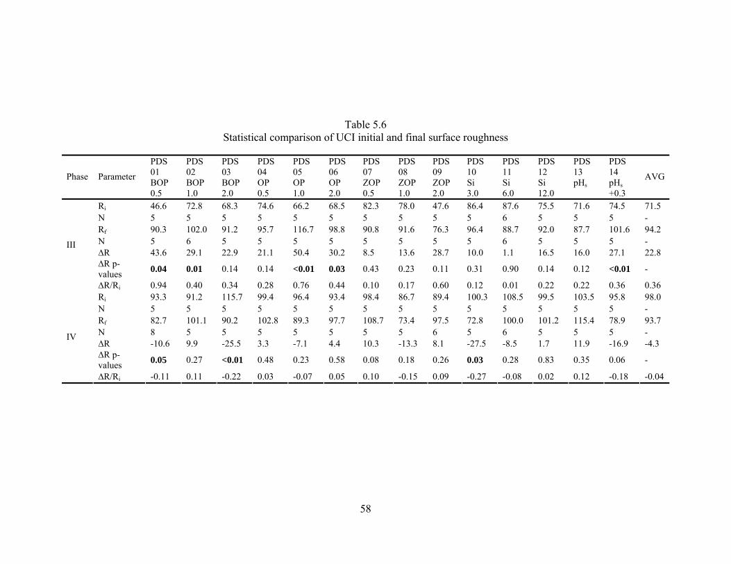
Table 5.6 Statistical comparison of UCI initial and final surface roughness

PDS 01

PDS 02

PDS 03

PDS 04

PDS 05

PDS 06

PDS 07

PDS 08

PDS 09

PDS 10

PDS 11

PDS 12

PDS 13

PDS 14 Phase Parameter BOP

0.5 BOP 1.0

BOP 2.0

OP 0.5

OP 1.0

OP 2.0

ZOP 0.5

ZOP 1.0

ZOP 2.0

Si 3.0

Si 6.0

Si 12.0

pHs

pHs +0.3

AVG

Ri 46.6 72.8 68.3 74.6 66.2 68.5 82.3 78.0 47.6 86.4 87.6 75.5 71.6 74.5 71.5 N 5 5 5 5 5 5 5 5 5 5 6 5 5 5 - Rf 90.3 102.0 91.2 95.7 116.7 98.8 90.8 91.6 76.3 96.4 88.7 92.0 87.7 101.6 94.2 N 5 6 5 5 5 5 5 5 5 5 6 5 5 5 - ∆R 43.6 29.1 22.9 21.1 50.4 30.2 8.5 13.6 28.7 10.0 1.1 16.5 16.0 27.1 22.8 ∆R p-values 0.04 0.01 0.14 0.14 <0.01 0.03 0.43 0.23 0.11 0.31 0.90 0.14 0.12 <0.01 -

III

∆R/Ri 0.94 0.40 0.34 0.28 0.76 0.44 0.10 0.17 0.60 0.12 0.01 0.22 0.22 0.36 0.36 Ri 93.3 91.2 115.7 99.4 96.4 93.4 98.4 86.7 89.4 100.3 108.5 99.5 103.5 95.8 98.0 N 5 5 5 5 5 5 5 5 5 5 5 5 5 5 - Rf 82.7 101.1 90.2 102.8 89.3 97.7 108.7 73.4 97.5 72.8 100.0 101.2 115.4 78.9 93.7 N 8 5 5 5 5 5 5 5 6 5 6 5 5 5 - ∆R -10.6 9.9 -25.5 3.3 -7.1 4.4 10.3 -13.3 8.1 -27.5 -8.5 1.7 11.9 -16.9 -4.3 ∆R p-values 0.05 0.27 <0.01 0.48 0.23 0.58 0.08 0.18 0.26 0.03 0.28 0.83 0.35 0.06 -

IV

∆R/Ri -0.11 0.11 -0.22 0.03 -0.07 0.05 0.10 -0.15 0.09 -0.27 -0.08 0.02 0.12 -0.18 -0.04

58

Conclusions

Optical profilometry can be used to measure surface roughness of pipe materials common

in water distribution systems, including galvanized iron, lined cast iron, polyvinyl chloride,

unlined cast iron. Corrosion inhibitor addition and water quality were not found to be significant

factors affecting G, LCI, and PVC surface roughness. UCI surface roughness appeared to be

influenced by phosphates, temperature, and alkalinity. For all materials, the most significant

factor influencing the change in surface roughness was the initial surface roughness. The initial

roughness varied greatly between materials. PVC was the smoothest material. LCI and G had

similar roughnesses, and UCI was the roughest material.

Recommendations

The development of standard methods for the measurement of surface roughness of

corrosion coupons by optical profilometry would help standardize the collection and

interpretation of results. An optical profiler could be used for further studies investigating the

relationship between surface roughness and biofilm density, chlorine wall decay rates, and

polyphosphate reversion.

Although, in this study, models did not indicate a statistically significant effect of

inhibitors on surface roughness over three months, similar studies with longer incubation times

for corrosion coupons, such as six months to one year, may demonstrate some effect.

Also, whereas the pilot distribution systems was operated to simulate dead end

conditions, similar studies operated under turbulent flow conditions may have different results

for iron surface roughness.

59

Head loss tests within the distribution system would be more sensitive to the practical

effect of corrosion inhibitors on surface roughness. A utility collecting Hazen-Williams

coefficients as part of hydrodynamic modeling efforts could compare head loss data before and

after introduction of inhibitors to directly measure the practical effect of inhibitors on pipe

surface roughness. If corrosion inhibitors had a beneficial effect on surface roughness of unlined

iron in the distribution system, then one would also expect to see decreases in energy

consumption for the high-service pumps and booster pumps throughout the system.

60

CHAPTER 6 SURFACE CHARACTERIZATION AND SOLUBILITY MODELING OF COPPER LOOPS RECEIVING PHOSPHATE INHIBITORS

Abstract

The effect of phosphate inhibitors on copper release in copper tubing receiving a varying

blend of ground, surface and brackish water was investigated. Blended poly/ortho phosphate,

sodium orthophosphate, and zinc orthophosphate were used from about 0.5 to 2 mg P/L and

reduced copper release compared to the no inhibitor pH controls at pHs and pHs+0.3.

All phosphate inhibitors reduced copper release relative to the no inhibitor treatments,

keeping total copper below the 1.3 mg/L MCLG for all water quality blends. Addition of 1 mg/L

as P phosphorus reduced both total and dissolved copper by about 60% relative to no inhibitor

addition. This effect was consistent even with seasonal changes in source water blends.

Solubility models were developed to predict copper release concentration assuming Cu(OH)2 or

Cu(PO4)3 as the controlling solid phase. The Cu(OH)2 model consistently under predicted copper

release for pH controls whereas the Cu2(PO4)3 model adequately fit the data for P inhibitors.

A plot of cupric ion concentration versus orthophosphate concentration showed a

decrease in copper release consistent with mechanistic control by either cupric phosphate

solubility or a diffusion limiting phosphate film.

61

Introduction

Management of water quality in distribution systems is an essential task for utilities to

deliver a reliable supply of drinking water that meets consumer expectations and complies with

regulatory requirements. It is desirable for utilities to find a corrosion control strategy that can

mitigate copper release below LCR action levels despite seasonal variations in source water

quality, which can potentially disrupt existing copper scales. A recent AwwaRF study entitled

“Control of Distribution System Water Quality in a Changing Water Quality Environment Using

Inhibitors” (Taylor et al., 2007) investigated the use of corrosion inhibitors to mitigate adverse

impacts of varying water quality in distribution systems receiving seasonally varied source water

blends. Significant decreases in copper release were observed with the addition of phosphate or

silicate inhibitors.

This paper examines the effect of phosphate inhibitors on copper release. Surface

characterization and water quality data were used to evaluate possible mechanisms whereby

phosphate inhibitors reduced copper release.

Copper Corrosion

Copper corrodes from its noble metallic form of Cu0 to the, cuprous, Cu(I) and cupric,

Cu(II) ions. The maximum contaminant level goal (MCLG) and action level for LCR compliance

for copper in potable water systems is 1.3 mg/L. Elevated copper can cause gastrointestinal

distress, liver damage, and/or kidney damage (Barceloux and Barceloux 1999).



62



copper (II).


article; which investigated treatment process impacts on water quality without use of inhibitors.

Cuprite (Cu2O) was identified as a crystalline structure found in the corrosion layer using XRD

(Taylor et al.; 2005). Cupric hydroxide (Cu(OH)2), tenorite (CuO), and cuprite (Cu2O), made up

the bulk surface composition on copper coupons identified by XPS. Thermodynamic modeling

indicated that copper release was well described by equilibrium with Cu(OH)2 acting as the

controlling solid (Xiao; 2004). Alkalinity increased copper release; whereas pH elevation above

pHs and silica reduced copper release.

Often, in domestic systems, copper concentrations do not fully reach equilibrium between

use. It can take 48 to 72 hours to reach equilibrium copper levels in a disinfected copper loop

(Schock, Lytle, and Clement 1995). The authors also suggested that orthophosphate would be

most effective in controlling copper release in the pH range of 6.5 to 7.5. Orthophosphate

inhibitors are suggested to function by forming a cupric phosphate scale (Edwards, McNeill, and

Holm 2001); however, data on cupric phosphate solids is scarce (Schock, Lytle, and Clement

1995).

When inhibitors are not added, other methods for controlling copper release include

raising the pH, and or reducing the alkalinity. CO2 stripping has been recommended as one way

to increase the pH without increasing alkalinity (Edwards, Hidmi, and Gladwell; 2003).

However, decreasing the alkalinity can increase lead solubility (Taylor et al. 2005). Inhibitors are

63

an attractive alternative as they may overcome the apparent tradeoff between control of copper or

lead release concentration.

64


Pilot Testing

A pilot testing facility comprised of pilot distribution systems (PDSs), copper corrosion

loops, and PVC pipe cradles to house corrosion and biological coupons were used to test the

effects of corrosion inhibitors on distribution system water quality. The pilot testing facility was

located on the grounds of the Cypress Creek Water Treatment Facility , located in Pasco County,

Florida, USA.

Source Waters

Blends of surface water, groundwater, and brackish water were used for the pilot study.

Surface water was treated at a surface water treatment plant by ferric sulfate coagulation and

trucked to the pilot testing site. On site, additional surface water treatment process included

chloramination and pH stabilization. Raw groundwater was obtained from the Cypress Creek

water treatment facility. The groundwater treatment process included aeration, chloramination,

and pH stabilization. Brackish water was artificially prepared from the raw groundwater by the

addition of sea salt after RO treatment. The reverse osmosis desalinated water (RO) treatment

process included reverse osmosis, aeration, chloramination, and pH stabilization.


tanks shown in Figure 6.1. Three blends were studied over four operating phases, with each

phase lasting three months. Within each phase, all pilot distribution systems received the same

blend of water. Blend composition, water quality, and schedule for each phase are presented in

Table 6.1.

65




2-) 62 103 67 76 Temperature (°C) 21.3 26.2 25.7 21.2



Blended poly/ortho phosphate (BOP), orthophosphate (OP), zinc orthophosphate (ZOP),

and silicate (SiO2) were fed from inhibitor tanks by peristaltic pumps, into influent standpipes to

mix with blended water coming from the process storage tanks. Phosphate inhibitors were dosed

at 0.5, 1.0, and 2.0 mg/L as P, while silicate inhibitor was dosed at 3.0, 6.0, and 12.0 mg/L as

SiO2. Two PDSs were operated as pH controls without inhibitor addition, one at the stability pH

for calcium carbonate precipitation i.e. pHs, while the other at an elevated pH of pHs+0.3.





PDSs were excavated from TBW member government distribution systems. The 14 hybrid PDSs

each about 92 feet long ,consisted of polyvinylchloride (PVC), lined cast iron (LCI), unlined cast

iron (UCI) pipe, and galvanized iron (G) in series.

66

Copper Loops

Copper loops were housed (Figure 6.3) in series at the end of each PDS to simulate a

home plumbing system. Copper tubes (Figure 6.4) were 5/8 in. (1.6 cm) in diameter and 30 ft.

(9.1 m) in length. Copper loops were flushed every morning with 2 gallons (7.6 L) of water at an

average velocity of 1 fps. Copper concentration was measured weekly from water from copper

loops after a standing time of six to seven hours.


Figure 6.3 Corrosion shed Figure 6.4 Copper lines

67


Chemical composition of corrosion scales on the surface of metal coupons copper

exposed to the various inhibitors were characterized by XPS or X-ray Photoelectron

Spectroscopy (Physical Electronics 5400 ESCA) shown in Figure 6.5. In XPS, an Mg anode

(1254 eV kα) bombards the coupon surface with high energy X-rays that interact with atoms in

the top 5-6 nm of the surface (Seal and Barr 2001). Then, according to the photoelectric effect,

these atoms emit high energy electrons. An electron analyzer counts the number of electrons

emitted over a range of energies, producing scan spectra which may be used for surface

composition analysis.

The effluent from the PDS was split in two parts. One part was directed to the copper

corrosion loops and the other was directed to a trailer which housed electrochemical noise

electrodes and copper corrosion coupons. These coupons were inserted at the beginning of each

phase, and then retrieved at the end of the phase, about 90 days later The XPS scanning consists

of a two-step process: an initial “survey” scan followed by a “high resolution” scan. The survey

scan, conducted over a broad range of energy levels, is useful for confirming the presence or

absence of elements on the surface of the coupon. In contrast, a high resolution scan, conducted

over a narrow range of energy levels, is useful for establishing the chemical states present for a

given element.

68

Figure 6.5 Physical Electronics 5400 ESCA XPS

The elements are indicated on the survey scan by pronounced peaks above the

background of the survey, and these peaks are then selected individually for a “high resolution”

scan for each element. Additionally, elements of interest, such as those associated with

inhibitors, coupon material, or water quality, were analyzed with high resolution scans. Possible

compounds associated with a given element were determined through deconvolution of the high

resolution scan.


Cu(OH)2 has been identified as a metastable intermediate that forms in new copper pipe,

and has been used as the basis for thermodynamic models of copper (Schock, Lytle, and Clement

1995)(Xiao 2004). Cupric hydroxide can age to its dehydrated form tenorite, CuO, which is less

soluble. In the presence of alkalinity, old copper pipe tends to form the more stable, less soluble

cupric hydroxycarbonate Cu2(OH)2CO3, malachite (Schock, Lytle, and Clement. 1995). Cupric

69

phosphate has also been identified as a possible controlling solid for copper release in the

presence of phosphate inhibitors.

Thermodynamic Model Development

The thermodynamic model for dissolved copper that had been developed in TBW I

(Taylor et al., 2005) was expanded to include phosphate, sulfate, chloride, and ammonia

complexes and is given in Equation 6.1. The equilibrium model assumed the presence of Cu (II)

species. Silica complexation of copper was also considered; however, a review of literature

concerning coordination chemistry did not reveal any thermodynamic data corresponding to a

copper-silica complex.

[ ] [ ] ( )[ ] ( )[ ] [ ] [ ]( )[ ] ( )[ ] ( )[ ] [ ]

[ ] [ ] ( )[ ] ( )[ ] ( )[( )[ ] ( )[ ] [ ] [ ]o

oo

oo

CuClCuClNHCuNHCu




++++

+++++

++++

+++++=

+++

+++

+−−−

+−++

253

243

233

223

2344

422323

23

33322

T CuCu

] Equation 6.1

The complexes considered within Equation 6.1 demonstrate the various water quality

parameters governing copper release. The free dissolved cupric ion concentration at equilibrium

depends on the controlling solid; however, other water quality parameters, such as alkalinity,

chloride, sulfate, ammonia, and phosphate form copper complexes in equilibrium with the free

cupric ion, and thus amplify the natural level of dissolved copper. Empirical models developed

as a part of this study, and reported elsewhere (Taylor et al. 2007) identified pH, chloride, and

alkalinity as the main water quality effects. Increased pH was beneficial in controlling copper

release, whereas increasing the chlorides or alkalinity increased copper release.

70

The effect of chlorides on dissolved copper did not appear to be explained by formation

of a copper-chloride complex., because CuCl+ and CuClo complexes accounted for

approximately 1/1000th of a percent of the dissolved copper. Rather, the effect may relate to

associated changes in solution conductivity and ionic strength that accompany elevated chloride

concentrations. It is speculated that chlorides may have reduced carbonate/ hydroxide scale

passivity by promoting local pH drops near copper surfaces and may cause pitting corrosion;

however for the moderate alkalinity (84-175 as CaCO3) waters used in this study large pits were

not observed on copper surfaces.

For this study, copper-alkalinity complexes accounted for approximately 90% of all

dissolved copper. Copper-alkalinity complexes included CuHCO3-, CuCO3

o, Cu(CO3)22-,

Cu(OH)CO3-, and Cu(OH)2CO3

2-. Equilibrium calculations demonstrated that alkalinity had a

tremendous effect on copper release, capable of increasing the total dissolved copper to several

times the level of free dissolved copper.

For this study, copper-phosphate complexes accounted for only about 0.5% of total

dissolved copper, indicating little adverse effect. Copper-phosphate complexes included

CuH2PO4+ and CuHPO4

o.

Model Implementation

Separate runs of the model were performed assuming considering the following

compounds as candidate controlling solids: cupric hydroxide (Cu(OH)2), tenorite (CuO), and two

forms of cupric phosphate, Cu3(PO4)2 and its dihydride Cu3(PO4)2 2H2O. Calculations were

performed for the pHs controls and all phosphate inhibitor types using average water quality data

71

for each phase. The middle dose (1.0 mg/L as P) phosphate inhibitor lines were modeled which

corresponded with the coupons tested by XPS analysis.

Mechanistic Investigation of Copper Release

Water quality data for copper release were compared against two mechanistic models

derived from cupric phosphate solubility and from diffusion theory. The purpose of this

investigation was to identify the most plausible mechanism to explain the reduction in copper

release with phosphate inhibitor addition.

Solubility Model

If cupric phosphate solubility controlled dissolved copper, then the expected copper

concentration should vary as function of the orthophosphate concentration. Solving the solubility

product equation of cupric phosphate (Equation 6.2) for free dissolved copper yielded Equation

6.3 which predicted that free dissolved copper varied with the -2/3rd power of the orthophosphate

concentration.

[ ] [ 234

32 −+= POCuKsp ] Equation 6.2

[ ] [ ]

31

234

2

⎟⎟⎠

⎞⎜⎜⎝

⎛= −−

+

PO

KCu sp Equation 6.3

Under cupric phosphate control, the free dissolved copper would depend primarily on the

orthophosphate concentration, which is a function of the phosphoric acid concentration

(CT,PO4),and pH. In contrast, the total dissolved copper depends on the free dissolved copper and

the concentration of copper ligands, especially alkalinity. Free dissolved copper concentrations

were solved using the water quality data and back calculating with complexation coefficients

72

assembled by Shock, Lytle, and Clement (1995). Hence, instead of total dissolved copper, it is

most appropriate to consider a plot of free dissolved copper versus orthophosphate, because the

effect of alkalinity is removed. If cupric phosphate acts as a controlling solid for copper release,

then the data should be consistent with a -2/3rd order power model like that shown in Equation

6.4.

[ ] [ ] 3234

2 −−+ ×= POaCu Equation 6.4

Film Diffusion Model

If cupric phosphate was not the controlling solid for copper release, then phosphate

inhibitor addition may have reduced copper release by formation of a film over the controlling

copper solid. Whatever the composition of this phosphate film, the film thickness might be

approximated as a linear function of the orthophosphate concentration. Hence, increased

phosphate inhibitor addition would result in thicker phosphate films, which would reduce the rate

of diffusion of dissolved copper to the bulk.

Fick’s first law (Equation 6.5), describes the diffusion flux, J, as a function of a diffusion

coefficient, D, and concentration gradient dxdφ . The negative sign indicates that the diffusion

flux goes against the concentration gradient.

dxdDJ φ

−= Equation 6.5

where: J = diffusion flux (ML-2T-1) D = diffusion coefficient (L2/T) φ = concentration (ML-3) x = position (L)

Applying this equation to copper diffusion through a phosphate film an equation

(Equation 6.6) describing the effect of phosphate film thickness on free dissolved copper was

73

developed. This equation assumes that the copper diffusion flux is directly proportional to the

dissolved copper in the bulk. It also assumes that the film thickness is directly proportional to the

orthophosphate concentration.

[ ] [ ][ ]−

++

+= 3

4

22

1 POaCu

Cu surfacebulk Equation 6.6

where: [ ]bulkCu +2 = dissolved copper concentration in the bulk (ML)

[ ]surfaceCu +2 = dissolved copper concentration at the copper surface (ML) a = proportionality constant [ ]−3

4PO = orthophosphate concentration in the bulk (ML-3)

74


Effect of Phosphate Inhibitor on Copper Release

The average copper release observed during the study is shown in Table 6.2 by phase for

each phosphate inhibitor and relative to the pHs+0.3 control. In all cases, inhibitors reduced

copper release relative to the control. Phosphate inhibitors reduced copper release to about 40%

that observed with the control. Time series plots for BOP, OP, ZOP, and the no inhibitor controls

are shown in Figure 6.6through Figure 6.9. The plots show that the addition of 0.5, 1.0, or 2.0

mg/L as P of phosphate inhibitor tended to reduce copper release in proportion to the copper

release observed with the no inhibitor control pHs+0.3.

Table 6.2 Comparison of observed copper release from inhibitor PDSs to pHs+0.3

Average Release (mg/L) % Ratio to pHs+0.3 Phase Inhibitor Dissolved Cu Total Cu Dissolved Cu Total Cu

pHs+0.3 0.89 1.00 BOP 0.34 0.36 38% 36% OP 0.38 0.41 42% 41%

I

ZOP 0.34 0.36 38% 36% pHs+0.3 0.73 0.82

BOP 0.29 0.33 40% 40% OP 0.28 0.35 39% 43%

II

ZOP 0.32 0.39 44% 48% pHs+0.3 0.79 0.85

BOP 0.30 0.32 38% 38% OP 0.29 0.35 37% 41%

III

ZOP 0.30 0.34 37% 40% pHs+0.3 0.83 0.93

BOP 0.31 0.37 38% 39% OP 0.32 0.36 38% 39%

IV

ZOP 0.32 0.38 38% 41%

75

Figure 6.6 Time series plot of copper release with BOP inhibitor addition

Figure 6.7 Time series plot of copper release with OP inhibitor addition

76

Figure 6.8 Time series plot of copper release with ZOP inhibitor addition

Figure 6.9 Time series plot of copper release by pH without inhibitor addition

77

XPS Identification of Copper Corrosion Products

An example XPS survey spectrum for copper is shown in Figure 6.10. Peaks were

dependent on the inhibitor to which the coupon had been exposed and were typically pronounced

for copper, carbon, oxygen, calcium, phosphorus, and zinc.

Binding Energy (eV)

N(E)

Min: 89 Max: 10298

1100 990 880 770 660 550 440 330 220 110 0

Ca 2p3

Zn 2p3

Cu 2p3

P 2p3C 1s

O 1s

Figure 6.10 Survey spectrum of a copper coupon from 1.0 ZOP, Phase III

Identification of Copper Corrosion Products

High resolution spectra for copper were deconvoluted (Figure 6.11) to identify copper

corrosion products and to determine their relative abundance. Copper compounds detected

included: Cu2O, CuO, Cu(OH)2; and cupric salts Cu(II) (Xiao, 2004). Binding energy data from

the NIST database (Wagner et al.,; 2003) support the inclusion of CuCl2, CuSO4, CuCO3, and

CuSiO3 under the Cu (II) curve given by Xiao (2003). In addition Cu3(PO4)2, Cu2(OH)2CO3

78

(malachite), and Cu4SO4(OH)6H2O (a cupric hydroxysulfate) are all feasible cupric salts

(Schock, Lytle, and Clement 1995); however, no published XPS binding energies were identified

for these compounds. It should be noted that the surface composition of copper coupons is not

uniform. Failure to detect a compound by XPS in one scan did not imply the compound was not

likely to be present in the scale.

Binding Energy (eV)

N(E)

Min: 0 Max: 9802

948 946 944 942 940 938 936 934 932 930 928

Curve Fit Summary# Comment Area Area% Position Intensity FWHM1 Cu2O 5264 12.5% 932.00 3372 1.402 CuO 10943 25.9% 933.17 5576 1.763 Cu(OH)2 19779 46.8% 934.51 7095 2.504 Cu (II) 6247 14.8% 935.91 2630 2.13

1Cu2O

2CuO

3Cu(OH)2

4Cu (II)

Figure 6.11 Deconvolution of copper for the coupon exposed to BOP during Phase IV

A combination of these four compounds was sufficient to describe the high resolution

spectra for the copper coupons. Figure 6.12 depicts the percent area of the various compounds

over all phases by inhibitor treatment. Cupric hydroxide was the most abundant copper surface

compound. This may imply that Cu(OH)2 was the controlling solid phase for copper solubility

(Schock, 1999)(Xiao, 2004). However, as shown in the thermodynamic models for copper, the

cupric phosphate dihydride, Cu3(PO4)2·2H2O model provided reasonable predictions of dissolved

79

copper release from copper loops receiving phosphate inhibitors. It should be noted that this

compound corresponds stoichiometrically with a cupric biphosphate dihydroxide,

CuHPO4(OH)2, solid. This may indicate that biphosphate plays a role in the controlling solid for

copper release. Cu(OH)2 commonly forms in new copper pipe. Tenorite is more

thermodynamically stable than cupric hydroxide; however, the rate of transformation of cupric

hydroxide to tenorite is slow, resulting in cupric hydroxide being present as a metastable

intermediate. Older copper pipe tends to form the more stable, less soluble cupric

hydroxycarbonate Cu2(OH)2CO3, malachite (Schock, Lytle, and Clement; 1995); nonetheless,

increased levels of alkalinity can aggravate copper release (Taylor et Al.,; 2005), even in older

copper pipe (Schock and Fox; 2001). This results is reasonable since the primary effect of

alkalinity on cuprosolvency is to multiply copper concentrations by complexing free dissolved

copper. Changes in the controlling solid phase with ageing of copper pipe may reduce the free

uncomplexed dissolved copper; however, the effect of alkalinity on dissolved copper is largely

independent of the controlling solid phase since it acts to increase dissolved copper by

complexing cupric ions already in solution.

80

0%

10%

20%

30%

40%

50%

60%

70%

80%

90%

100%

BOP OP ZOP Si pH

Inhibitor

% A

rea

of C

ompo

und

Cu(II) Cu(OH)2 Cu2O CuO

Figure 6.12 Distribution of copper compounds for all phases

Effect of Inhibitor on Copper Scale Corrosion Products

Copper coupons exposed to BOP, OP, and ZOP were analyzed for the elements shown in

Table 6.3. One copper coupon was tested for each phase. For brevity, only the results of OP are

presented. The main differences observed with BOP and ZOP inhibitors were the presence of

polyphosphates and zinc oxides respectively.

Phosphate Inhibitor. For the OP coupons, carbon was detected in the copper scale on

four out of four coupons as carbonate. Calcium was detected on two out of four coupons as

CaCO3 in Phase I and in Phase III. This indicated that in the presence of a similar predominantly

groundwater blend conditions may favor the formation of CaCO3 films. Other calcium

compounds, such as Ca3(PO4)2 were not detected on copper coupons in the presence of OP

inhibitor.

81

Table 6.3 Compounds identified in scale on copper coupons in the presence of OP inhibitor

Element Compound Phase I Phase II Phase III Phase IV C CO3

2- X X X X Ca CaCO3 X X

Ca3(PO4)2 CaO

Cu Cu2O X X X X CuO X X X X Cu(OH)2 X X X X Cu(II) X X X

O O2- X X X X CO3

2- X X X X OH- X X X X PO4

3- X X X P PO4

3- X X X Meta Pyro

Si Zn ZnO X

Copper was detected on four out of four coupons, as a mixture of Cu2O, CuO, Cu(OH)2,

and Cu(II) salts, except for Phase I. Cu(II) salts were not detected on the copper coupon for

Phase I. In Phases, II, III, and IV, Cu (II) may be present as a copper carbonate compound, such

as CuCO3 or Cu2(OH)2CO3, since carbonate was detected for all these phases, but calcium was

detected only in Phase III. Similarly, since it is not precipitated with calcium, phosphate may be

present as Cu2(PO4)3. However, it is also possible that phosphate was adsorbed to the scale

surface as a liquid-solid film. Oxygen was detected on four out of four coupons as a mixture of

O2-, CO32-, OH-, and PO4

3-, except for Phase IV. PO43- was not detected on the copper coupon for

Phase IV. This result was consistent with observations for BOP, where PO43- was not detected on

the copper coupon in Phase IV.

82

Phosphorus was detected on three out of four coupons as PO43- in Phases I, II, and III

only. Phosphorus was not detected on the Phase IV coupon, which is consistent with the results

for oxygen. As mentioned in the thermodynamic modeling section, phosphate may also be

present as a copper phosphate solid. Although the actual form of such a solid in distribution

systems has not been established in the literature, the thermodynamic model for Cu3(PO4)2·2H2O

gave reasonable predictions for dissolved copper release for all phosphate inhibitors. Silica was

not detected on any of the four coupons. Zinc was detected on one of the four coupons, found in

the form of ZnO, for Phase III. This zinc might have come from the G pipe section of the PDSs

which was upstream of the PVC pipe which housed these corrosion coupons. .

No Inhibitor - pH control. Four copper coupons exposed to the pHs+0.3 treatment were

analyzed for the elements shown in Table 6.4. One copper coupon was tested for each of the four

phases. Carbon was detected on four out of four coupons, always appearing as carbonate.

Calcium was not detected on the four coupons tested, indicating that CaCO3 films were not

formed in the absence of phosphate and/or silicate inhibitors.

Copper was detected on four out of four coupons as a mixture of Cu2O, CuO, Cu(OH)2,

and Cu(II) salts, for all phases. Cu (II) salts may be present as a cupric carbonate compound such

as CuCO3 or Cu2(OH)2CO3, given that CO32- is present, and no significant calcium was detected.

Oxygen was detected on four out of four coupons as a mixture of O2-, CO32-, and OH-. It should

be noted that PO43- was not detected on any of the four coupons for the pHs treatment,

confirming that phosphate inhibitor addition is the primary source for phosphorus on the copper

surfaces for the given water qualities studied.

Phosphorus was detected on none of the four coupons, consistent with the results from

oxygen. Silica was not detected on the four coupons tested, indicating that silicate inhibitor

83

addition is the primary source for crystalline silicate compounds on the copper surfaces for the

given water qualities studied. Zinc was not detected on any of the four coupons.

Table 6.4 Compounds identified in scale on copper coupons in the presence of pHs+0.3 treated waters

Element Compound Phase I Phase II Phase III Phase IV C CO3

2- X X X X Ca CaCO3 X

Ca3(PO4)2 CaO

Cu Cu2O X X X X CuO X X X X Cu(OH)2 X X X X Cu(II) X X X X

O O2- X X X X CO3

2- X X X X OH- X X X X PO4

3- P PO4

3- Meta Pyro

Si Zn

Four copper coupons exposed to the pHs+0.3 treatment were analyzed for the elements

shown in Table 6.4. One copper coupon was tested for each of the four phases. Carbon was

detected on four out of four coupons, always appearing as carbonate. Calcium was detected on

one of the four coupons, appearing in Phase IV as CaCO3. This result is counterintuitive given

the lower calcium and alkalinity levels of Phase IV.

Copper was detected on four out of four coupons, appearing as a mixture of Cu2O, CuO,

Cu(OH)2, and Cu(II) salts, for all phases. Cu (II) salts may be present as a cupric carbonate

compound such as CuCO3 or Cu2(OH)2CO3, given that CO32- is present, and no significant

84

calcium was detected in Phases I, II, and III. Oxygen was detected on four out of four coupons,

appearing as a mixture of O2-, CO32-, and OH-. No PO4

3- was detected on any of the four coupons

for the pHs+0.3 treatment, establishing that phosphate inhibitor addition is the primary source for

phosphorus on the copper surfaces for the given water qualities studied. Phosphorus was detected

on none of the four coupons, consistent with the results from oxygen.

Silica was not detected on the four coupons tested, indicating that silicate inhibitor

addition is the primary source for crystalline silicate compounds on the copper surfaces for the

given water qualities studied. Zinc was not detected on any of the four coupons. Similar results

were observed for the pHs treatment except CaCO3 was not detected and Cu2O was not detected

in Phase III.


Expected Copper Release from Thermodynamic Models

pHs+0.3. Table 6.2 compared copper release observed with inhibitor addition to copper

release observed with the initial source water. A thermodynamic model was developed to

consider copper release as a function of a copper controlling solid phase. The prediction of

copper release was determined form the previously defined thermodynamic model for copper

release.

From the XPS analysis, it was determined that cupric hydroxide (Cu(OH)2was the

predominant copper corrosion product present on the copper coupons. Tenorite (CuO), cuprous

oxide (Cu2O), and cupric salts (Cu(II)) were also present on the copper coupons.

Binding energy data from the NIST database (Wagner et al. 2003) support the inclusion

of CuCl2, CuSO4, CuCO3, and CuSiO3 under the Cu (II) curve given by Xiao. In addition

85

Cu3(PO4)2, Cu2(OH)2CO3 (malachite), and Cu4SO4(OH)·6H2O (a cupric hydroxysulfate) are all

feasible cupric solids (Schock, Lytle, and Clement 1995); however, no published XPS binding

energies were identified for these three compounds.

Both cupric hydroxide and tenorite were considered as the controlling solid phase during

thermodynamic modeling. Table 6.5 shows that the cupric hydroxide thermodynamic model

under-predicted the dissolved copper concentrations by about 0.3 mg/L Cu. Similarly, the

tenorite thermodynamic model under-predicted the dissolved copper concentrations by about 0.7

mg/L Cu. Equation 6.7 describes the equilibrium of dissolved cupric ion with cupric hydroxide

solids. A log equilibrium constant of 8.89 was used to predict copper dissolution from cupric

hydroxide scales. This same value has been used in other studies modeling cupric hydroxide as a

controlling solid phase for copper release (Shock, Lytle, and Clement 1995) (Xiao 2004).

OHCuHOHCu s 22

)(2 22)( +↔+ ++

Equation 6.7

Table 6.5 Copper thermodynamic modeling of pHs+0.3

Actual Copper Release (mg/L) Modeled Copper Release (mg/L) Inhibitor Phase

Diss Cu Total Cu Cu(OH)2 CuO

pHs+0.3 1 0.89 1.00 0.59 0.07 2 0.73 0.82 0.46 0.06 3 0.79 0.85 0.48 0.06 4 0.83 0.93 0.54 0.07 All 0.81 0.90 0.54 0.07

The dissolved copper samples were collected six hours after flushing of the copper loops,

and six hours is less than the time required for copper concentrations to reach equilibrium values

86

(Schock, Lytle, and Clement; 1995). In both this study and TBW I (Taylor et al.,; 2007, 2005),

which were conducted using the same pilot distribution system and copper loops, the cupric

hydroxide model, with log equilibrium constant 8.89, consistently under-predicted dissolved

copper release (Xiao 2004). The variability of equilibrium constants for copper scales, including

copper hydroxide, was discussed by Schock, Lytle and Clement (1995). Using earlier work by

Schindler et al., (1965,1967) they found the range of log equilibrium constants for cupric

hydroxide to vary from 8.67 to 8.89, when corrected for ionic strength. Hidmi and Edwards

reported a log equilibrium constant of 9.36±0.02 for freshly precipitated Cu(OH)2 (1999).

The observed copper concentrations presented in these results are consistent with what

would be expected using a greater log equilibrium constant. The log equilibrium constant for

Cu(OH)2 has been observed to decrease with aging of the cupric hydroxide solids (Hidmi and

Edwards 1999). Other reported values for the Cu(OH)2 log equilibrium constant include 8.3, 8.7,

9.2, and 9.4 (King 1959) (Hahn and Welcher 1969) (Hogness and Johnson 1957) (Schenk 1996).

A unit variation in log equilibrium constant would result in a log order variation in predicted

copper release.

The dramatic reductions in copper release with the addition of phosphate inhibitor, as

shown in Table 6.2 , suggest that a less soluble copper phosphate solid may form; however, very

little information on solid forms of copper orthophosphate solids is available (Schock, Lytle, and

Clement 1995). A review of the literature confirmed the lack of information identifying copper

orthophosphate solids in water distribution systems. Thermodynamic data was available for the

two forms Cu3(PO4)2·2H2O and Cu3(PO4)2, hence these were used to model cupric phosphate

solubility (Shock, Lytle, and Clement 1995).

87

For the range of pH values considered in this study with phosphate inhibitors, 7.7-8.0,

tenorite (CuO), is thermodynamically favored; however, tenorite usually forms by aging of

cupric hydroxide (Cu(OH)2) solids. Tenorite was detected by XPS on copper coupons for all

inhibitors but not as abundant as cupric hydroxide. This indicates cupric solids are slow to reach

equilibrium form as CuO. Therefore cupric hydroxide solids can persist as a metastable solid

(Xiao 2004). Near pH 8, cupric phosphate dihydride, Cu3(PO4)2·2H2O and cupric hydroxide,

Cu(OH)2 have similar predicted copper solubility, indicating that neither compound is

thermodynamically favored over the other.

OP. Copper corrosion products identified by the XPS analysis for the four copper

coupons exposed to OP found Cu(OH)2, CuO, Cu2O and Cu (II) copper scales. However,

Cu(OH)2 and CuO were the most predominant scales. Orthophosphate was found on three of

four copper coupons. Calcium phosphate was not detected on any of these coupons, although

calcium carbonate was detected on two of the three coupons with orthophosphate present. The

formation of tenorite is thermodynamically favored, but this solid is not as abundant as cupric

hydroxide due to kinetic limitations. For these conditions, given available thermodynamic

constants, cupric hydroxide and cupric phosphate dihydride are equally favored

thermodynamically.

Equilibrium calculations are provided in Table 6.6 considering cupric hydroxide, tenorite,

cupric phosphate dihydride, and cupric phosphate as the possible controlling solid phases. From

Table 6.2 there is a clear improvement with the control of copper release with the addition of OP

when compared to pHs+0.3. Both cupric hydroxide and cupric phosphate dihydride solids over

predict the observed dissolved copper release.

88

If the effective log equilibrium constant for cupric hydroxide were elevated to be

consistent with observed dissolved copper release for pHs+0.3, then the cupric phosphate

dihydride model would explain the decrease in copper release with OP addition. No data on the

XPS binding energies for cupric phosphate dihydride were located in the literature; however,

they may be represented as part of the Cu (II) salts curve.

Table 6.6 Copper thermodynamic modeling of OP


Diss Cu Total Cu Cu(OH)2 CuO Cu3(PO4)2·2H2O Cu3(PO4)2

OP 1 0.38 0.41 0.56 0.07 0.67 2.88 2 0.28 0.35 0.52 0.06 0.41 1.75 3 0.29 0.35 0.53 0.07 0.63 2.70 4 0.32 0.36 0.64 0.08 0.47 2.01 All 0.32 0.37 0.60 0.07 0.56 2.42

Mechanistic Investigation of Copper Release

Figure 6.13 shows the results of the mechanistic analysis comparing the diffusion model

and the solubility model as explanations for the observed reductions in free dissolved copper

with increasing orthophosphate. Both models make predictions consistent with the data. The

phosphate film diffusion model (-1st order) tends to under predict copper when orthophosphate is

greater than about 0.04*106 mg/L as P; however, the cupric phosphate solubility model (-2/3rd

order) appears to better fit the data within this range. Both models provided a plausible

description of the reduction in copper concentration with increasing phosphate inhibitor dose.

However, the low concentrations of orthophosphate ion near pH 8, suggest that biphosphate ion,

HPO42-, may play a more important role in inhibition of copper release.

89

Figure 6.13 Comparison of diffusion model and solubility model as mechanisms for the effect of orthophosphate on copper Release

90

Conclusions

A yearlong investigation of the effects of phosphate inhibitors on copper release was

undertaken using a specially constructed pilot plant and array of pilot distribution systems. The

effect of inhibitors was investigated under a range of blended waters including groundwater,

surface water, and reverse osmosis desalinated water.

Pilot distribution systems were tested with phosphate inhibitors including blended

poly/orthophosphate, sodium orthophosphate, and zinc orthophosphate and waters that had

received no inhibitors. On average, all phosphate inhibitors tended to reduce copper release by

about 60% at a 1 mg/L as P dose. This effect was consistent, even with seasonal changes in the

source water blend.

Surface characterization of copper coupons by x-ray photoelectron spectroscopy (XPS)

indicated that Cu2O, CuO, Cu(OH)2, and cupric salts were the main copper compounds on the

surface of the copper coupons. Orthophosphate was found on all copper coupons exposed to

phosphate inhibitors. A lack of published XPS binding energies precluded positive identification

of Cu2(PO4)3; however, Ca3(PO4)2 was ruled out by XPS analysis as the phosphate compound.

Thermodynamic models for copper release, based on Cu(OH)2, CuO, Cu3(PO4)2, and its

dihydride, Cu3(PO4)2 2H2O controlling solids were developed using reported thermodynamic

data. In all cases, copper-alkalinity complexes accounted for about 90% of predicted dissolved

copper. The Cu(OH)2 model was the closest fit for the no inhibitor line; however, it tended to

under predict copper concentrations. Considerable variation in Cu(OH)2 solubility products has

been reported in the literature.

Cu(OH)2 and Cu3(PO4)2 2H2O models provided similar copper release predictions for

copper loops receiving phosphate inhibitors. However, when the results with Cu(OH)2 and the no

91

inhibitor loops are considered, the cupric phosphate dihydride model provides the closest

prediction of copper release. The cupric phosphate dihydride solid corresponds

stoichiometrically with a cupric biphosphate dihydroxide, CuHPO4(OH)2, solid. The role of

biphosphate in the effect of phosphate inhibitors should be considered since it is the predominant

phosphate species at 7.2<pH<12.3.

Two mechanisms were proposed to explain how phosphate inhibitors control copper

release: a diffusion model, and a solubility model. The diffusion model was derived from Fick’s

first law of diffusion, assuming that phosphate inhibitors form a film that acts as a diffusion

barrier over the underlying controlling solid and that the film thickness varies with

orthophosphate concentration. The solubility model was derived from the solubility product

equation for cupric phosphate. The free uncomplexed cupric ion concentration was calculated

from the dissolved copper using the water quality data and published thermodynamic data.

Orthophosphate concentration was calculated using the phosphoric acid concentration and pH. A

plot of both models against the data from the orthophosphate loops showed that the copper

concentration decreased in a manner consistent with control by either cupric phosphate solubility

or a diffusion limiting phosphate film.

92

CHAPTER 7 SURFACE CHARACTERIZATION AND SOLUBILITY MODELING OF COPPER IN WATER DISTRIBUTION SYSTEMS RECEIVING SILICATE

INHIBITORS

Abstract

A yearlong investigation of the effects of silicate inhibitor on copper release was

undertaken using a specially constructed pilot plant and array of pilot distribution systems. A

range of blended waters were used including groundwater, surface water, and reverse osmosis

desalinated water.

Pilot distribution systems were run comparing silicate inhibitor doses ranging from 3 to

12 mg/L as SiO2. treated with silicate inhibitor and waters that had received no inhibitors. When

compared to no inhibitor addition, silicate inhibitor addition at 6.0 mg/L as SiO2 reduced copper

release by about 25-40%.



surface of the copper coupons. Oxidized silicon (SiOx) was detected on copper coupons exposed

to phosphate inhibitors. A lack of published XPS binding energies precluded positive

identification of the silicon as an adsorbed silicate film or as cupric silicate.

Thermodynamic models for copper release, based on Cu(OH)2, CuO, and CuSiO3 H2O

were developed using published thermodynamic data. In all cases, copper-alkalinity complexes

accounted for about 90% of predicted dissolved copper. The Cu(OH)2 model was the closest fit

for the no inhibitor line; however, it tended to under predict copper concentrations.. The CuSiO3

H2O models provided the closest prediction of copper release for the silicate inhibitor line,

whereas the Cu(OH)2 model tended to under predict copper release. Solubility constants for

Cu(OH)2 have been reported to vary with particle size. 93

Introduction

This paper examines the effect of sodium silicate inhibitor on copper release. A recent

AwwaRF study entitled “Control of Distribution System Water Quality in a Changing Water

Quality Environment Using Inhibitors” (Taylor et al. 2007) investigated the use of corrosion

inhibitors to mitigate adverse impacts of varying water quality in distribution systems.

Significant decreases in copper release were observed with the addition of phosphate or silicate

inhibitors. Control of copper release was maintained even with changes in season and water

quality. Surface characterization and water quality data were used to evaluate possible

mechanisms whereby silicate inhibitors reduced copper release.

Copper Corrosion

Copper corrodes from its metallic form of Cu0 to the, cuprous, Cu(I) and cupric, Cu(II)

ions. The maximum contaminant level goal (MCLG) and action level for LCR compliance for

copper in potable water systems is 1.3 mg/L. Elevated copper can cause gastrointestinal distress,

liver damage, and/or kidney damage (Barceloux and Barceloux 1999). Hence, utilities have a

motivation to produce nonaggressive waters that will not result in excessive copper release.





copper (II).


paper which investigated treatment process impacts on water quality without use of inhibitors.

94

XRD identified cuprite (Cu2O) crystalline structures in the corrosion layer (Taylor et al., 2005).

Cuprite (Cu2O), cupric hydroxide (Cu(OH)2), tenorite (CuO), and, made up the bulk surface

composition on copper coupons identified by XPS. Thermodynamic modeling indicated that

copper release was well described by equilibrium with Cu(OH)2 acting as the controlling solid

(Xiao; 2004). Alkalinity increased copper release; whereas pH elevation above pHs and silica

reduced copper release.

Often, in domestic systems, copper concentrations do not fully reach equilibrium between

use. It can take 48 to 72 hours to reach equilibrium copper levels in a disinfected copper loop

(Schock, Lytle, and Clement 1995). When inhibitors are not added, other methods for controlling

copper release include raising the pH, and or reducing the alkalinity. CO2 stripping has been

recommended as one way to increase the pH without increasing alkalinity (Edwards, Hidmi, and

Gladwell; 2003). However, decreasing the alkalinity can increase lead solubility (Taylor et al.

2005). Inhibitors may overcome the apparent tradeoff between control of copper or lead release

concentration.

Silicate Inhibitors

The form of dissolved silica in water has not been clearly established; however, it does

not behave as a charged anion such as SiO32- or as a colloid (Hem 1971). In contrast, silicate

inhibitor manufacturers claim that a negatively charged silica monomer, represented as SiO32-

adsorbs as a surface film on anodic sites (PQ Corp 2001) High passivation doses during the first

month of dosing were recommended to help in formation of a passivating silicate film. The

formation of a film was supported by scanning electron microscopy and x-ray photoelectron

spectroscopy.

95

Because silicate acts as an anodic inhibitor, there is the danger that insufficient dosages

could result in incomplete coverage of the anodic areas, leading to pitting corrosion. Silicate

inhibitor films tend to be self-limiting and do not form thick layers (Vic et al. 1996).

96


Pilot Testing

A pilot testing facility comprised of pilot distribution systems (PDSs), copper corrosion

loops, PVC pipe cradles to house corrosion and biological coupons were used to test the effects

of corrosion inhibitors on distribution system water quality. The PDSs were located in Pasco

County, Florida, USA on the grounds of the Cypress Creek Water Treatment Facility.

Source Waters

Blends of surface water, groundwater, and brackish water was used for the pilot study.


trucked to the pilot testing site. On site, additional surface water treatment process included




addition of sea salt after RO treatment. The reverse osmosis desalinated water (RO) treatment

process included reverse osmosis, aeration, chloramination, and pH stabilization.


tanks shown in Figure 5.2. Three blends were studied over four operating phases, with each

phase lasting three months. Within each phase, all pilot distribution systems received the same

blend of water. Blend composition, water quality, and schedule for each phase are presented in

Table 5.1.

97




2-) 62 103 67 76 Temperature (°C) 21.3 26.2 25.7 21.2



Blended poly/ortho phosphate (BOP), orthophosphate (OP), zinc orthophosphate (ZOP),

and silicate (SiO2) were fed from inhibitor tanks by peristaltic pumps, into influent standpipes to

mix with blended water coming from the process storage tanks. Phosphate inhibitors were dosed

at 0.5, 1.0, and 2.0 mg/L as P, while silicate inhibitor was dosed at 3.0, 6.0, and 12.0 mg/L as

SiO2. Two PDSs were operated as pH controls without inhibitor addition, one at the stability pH

for calcium carbonate precipitation i.e. pHs, while the other at an elevated pH of pHs+0.3.



distribution systems (PDSs), shown in Figure 7.2. All pipes used in the PDSs were excavated

from distribution systems. The 14 hybrid PDSs each about 92 feet long ,consisted of

polyvinylchloride (PVC), lined cast iron (LCI), unlined cast iron (UCI) pipe, and galvanized iron

(G) in series.

98

Copper Loops



(9.1 m) in length. Copper loops were flushed daily with 2 gallons (7.6 L) of water at an average

velocity of 1 fps. Copper concentration was measured weekly from water from copper loops

after a standing time of six to seven hours.


Figure 7.3 Corrosion shed Figure 7.4 Copper lines

99


Chemical composition of corrosion scales on the surface of metal coupons copper

exposed to the various inhibitors were characterized by XPS or X-ray Photoelectron

Spectroscopy (Physical Electronics 5400 ESCA) following each phase of operations. In XPS, an

Mg anode (1254 eV kα) bombards the coupon surface with high energy X-rays that interact with

atoms in the top 5-6 nm of the surface (Seal and Barr 2001). Then, according to the

photoelectric effect, these atoms emit high energy electrons. An electron analyzer counts the

number of electrons emitted over a range of energies, producing scan spectra which may be used

for surface composition analysis

The effluent from the PDS was split in two parts. One part was directed to the copper

corrosion loops and the other was directed to a trailer which housed 4 in diameter PVC pipes

with copper corrosion coupons. These coupons were inserted at the beginning of each phase, and

then retrieved at the end of the phase. The XPS scanning consists of a two-step process: an initial

survey scan followed by a high resolution scan. The survey scan, conducted over a broad range

of energy levels, is useful for confirming the presence or absence of elements on the surface of

the coupon. In contrast, a high resolution scan is conducted over a narrow range of energy levels

is useful for establishing the chemical states present for a given element.

The elements are indicated on the survey scan by pronounced peaks above the

background of the survey, and these peaks are then selected individually for a “high resolution”

scan for each element. Additionally, elements of interest, such as those associated with

inhibitors, coupon material, or water quality, were analyzed with high resolution scans. Possible

compounds associated with a given element were determined through deconvolution of the high

resolution scan.

100



Cu(OH)2 has been identified as a metastable intermediate that forms in new copper pipe,

and has been used as the basis for thermodynamic models of copper (Schock, Lytle, and Clement

1995)(Xiao 2004). Cupric hydroxide can age to its dehydrated form tenorite, CuO, which is less

soluble. In the presence of alkalinity, old copper pipe tends to form the more stable, less soluble

cupric hydroxycarbonate Cu2(OH)2CO3, malachite (Schock, Lytle, and Clement. 1995).

Thermodynamic Model Development

The thermodynamic model for dissolved copper that had been developed in TBW I

(Taylor et al., 2005) was expanded to include phosphate, sulfate, chloride, and ammonia

complexes and is given in Equation 4.4. The equilibrium model assumed the presence of Cu (II)

species. Silica complexation of copper was also considered; however, a review of literature

concerning coordination chemistry did not reveal any thermodynamic data corresponding to a an

aqueous copper-silica complex.

[ ] [ ] ( )[ ] ( )[ ] [ ] [ ]( )[ ] ( )[ ] ( )[ ] [ ]

[ ] [ ] ( )[ ] ( )[ ] ( )[( )[ ] ( )[ ] [ ] [ ]o

oo

oo

CuClCuClNHCuNHCu




++++

+++++

++++

+++++=

+++

+++

+−−−

+−++

253

243

233

223

2344

422323

23

33322

T CuCu

] Equation 7.1

The complexes considered within Equation 4.4 demonstrate the various water quality

parameters governing copper release. The free dissolved cupric ion concentration at equilibrium

depends on the controlling solid; however, other water quality parameters, such as alkalinity,

chloride, sulfate, ammonia, and phosphate form copper complexes in equilibrium with the free

101

cupric ion, and thus amplify the natural level of dissolved copper. Empirical models developed

as a part of this study, and reported elsewhere (Taylor et al. 2007) identified pH, chloride, and

alkalinity as the main water quality effects. Increased pH was beneficial in controlling copper

release, whereas increasing the chlorides or alkalinity increased copper release.

The effect of chlorides on dissolved copper did not appear to be explained by formation

of a copper-chloride complex., because CuCl+ and CuClo complexes accounted for

approximately 1/1000th of a percent of the dissolved copper. Rather, the effect may relate to

associated changes in solution conductivity and ionic strength that accompany elevated chloride

concentrations. It is speculated that chlorides may have reduced carbonate/ hydroxide scale

passivity by promoting local pH drops near copper surfaces and may cause pitting corrosion;

however for the moderate alkalinity (84-175 mg/L as CaCO3) waters used in this study large pits

were not observed on copper surfaces.

For this study, copper-alkalinity complexes accounted for approximately 90% of all

dissolved copper. Copper-alkalinity complexes included CuHCO3-, CuCO3

o, Cu(CO3)22-,

Cu(OH)CO3-, and Cu(OH)2CO3

2-. Equilibrium calculations demonstrated that alkalinity had a

tremendous effect on copper release, capable of increasing the total dissolved copper to several

times the level of free dissolved copper.

For this study, copper-phosphate complexes accounted for only about 0.5% of total

dissolved copper, indicating little adverse effect. Copper-phosphate complexes included

CuH2PO4+ and CuHPO4

o.

102

Model Implementation

Separate runs of the model were performed assuming considering the following

compounds as candidate controlling solids: cupric hydroxide (Cu(OH)2), tenorite (CuO), and

cupric silicate hydride (CuSiO3 H2O). Calculations were performed for the pHs controls and all

phosphate inhibitor types using average water quality data for each phase. The middle dose (5.0

mg/L as SiO2) silicate inhibitor lines were modeled because the coupons from these lines are the

ones studied by XPS analyses.

103


Effect of Silicate Inhibitor on Copper Release

The average copper release observed during the study is shown in Table 7.2 by phase for

each inhibitor and relative to the pHs+0.3 control. In all cases, inhibitors reduced copper release

relative to the control. Phosphate inhibitors, at dose 1 mg/L as P, reduced copper release to

about 40% that observed with the control. Silicate inhibitors, at dose 6 mg/L as SiO2, reduced

copper release to about 70% of that observed with the control.

Time series plots for Si, and the no inhibitor controls are shown in Figure 7.5 and Figure

7.6. The plots show that the addition of 3, 6, or 12 mg/L as SiO2 of silicate inhibitor tended to

reduce copper release in proportion to the copper release observed with the no inhibitor control

pHs+0.3.

104

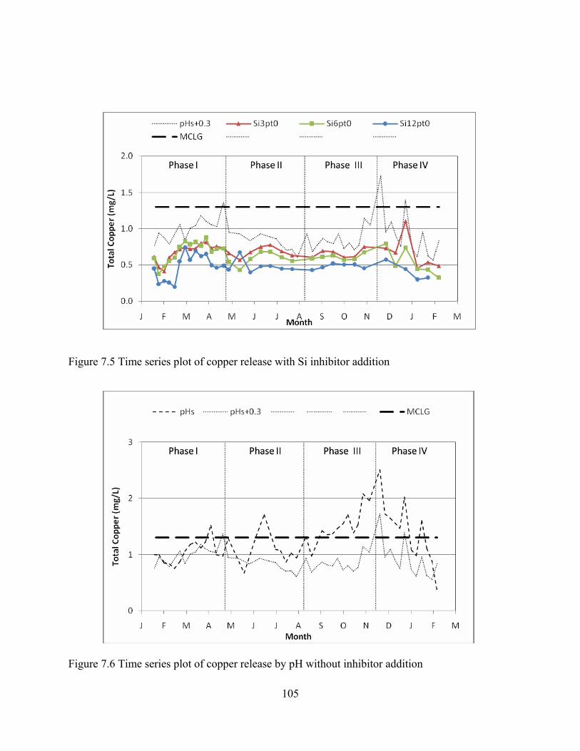
Figure 7.5 Time series plot of copper release with Si inhibitor addition

Figure 7.6 Time series plot of copper release by pH without inhibitor addition

105

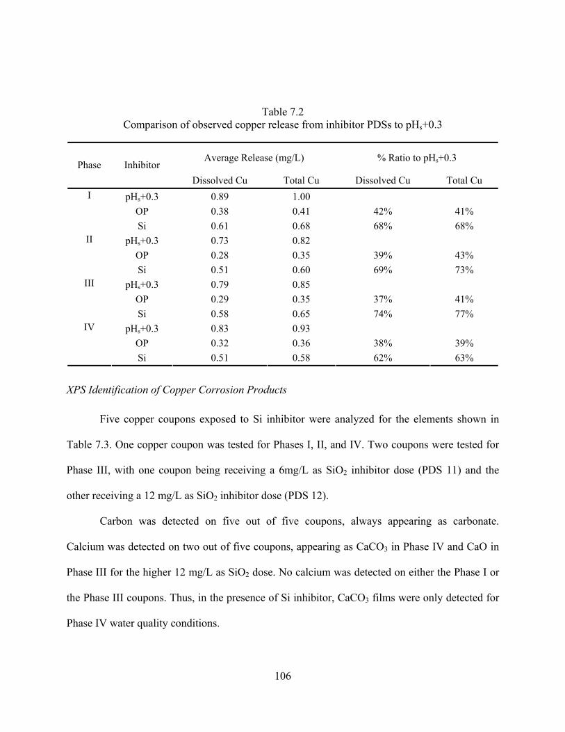
Table 7.2 Comparison of observed copper release from inhibitor PDSs to pHs+0.3

Average Release (mg/L) % Ratio to pHs+0.3 Phase Inhibitor

Dissolved Cu Total Cu Dissolved Cu Total Cu pHs+0.3 0.89 1.00

OP 0.38 0.41 42% 41% I

Si 0.61 0.68 68% 68% pHs+0.3 0.73 0.82

OP 0.28 0.35 39% 43% II

Si 0.51 0.60 69% 73% pHs+0.3 0.79 0.85

OP 0.29 0.35 37% 41% III

Si 0.58 0.65 74% 77% pHs+0.3 0.83 0.93

OP 0.32 0.36 38% 39% IV

Si 0.51 0.58 62% 63%

XPS Identification of Copper Corrosion Products

Five copper coupons exposed to Si inhibitor were analyzed for the elements shown in

Table 7.3. One copper coupon was tested for Phases I, II, and IV. Two coupons were tested for

Phase III, with one coupon being receiving a 6mg/L as SiO2 inhibitor dose (PDS 11) and the

other receiving a 12 mg/L as SiO2 inhibitor dose (PDS 12).

Carbon was detected on five out of five coupons, always appearing as carbonate.

Calcium was detected on two out of five coupons, appearing as CaCO3 in Phase IV and CaO in

Phase III for the higher 12 mg/L as SiO2 dose. No calcium was detected on either the Phase I or

the Phase III coupons. Thus, in the presence of Si inhibitor, CaCO3 films were only detected for

Phase IV water quality conditions.

106

Table 7.3 Compounds identified in scale on copper coupons in the presence of Si inhibitor

Element Compound Phase I Phase II Phase III (PDS 12) Phase IV C CO3

2- X X X(X) X Ca CaCO3 X

Ca3(PO4)2 CaO (X)

Cu Cu2O X X X(X) X CuO X X X(X) X Cu(OH)2 X X X(X) X Cu(II) X X X(X) X

O O2- X X X(X) X CO3

2- X X X(X) X OH- X X X(X) X PO4

3- P PO4

3- Meta Pyro

Si SiOx X (X) X Zn

Copper was detected on five out of five coupons, appearing as a mixture of Cu2O, CuO,

Cu(OH)2, and Cu(II) salts, for all phases. Cu (II) salts may be associated with carbonates

(detected for five out of five coupons), and cupric silicate (detected on three out of five coupons).

It has been suggested that CuSiO3 can form from malachite exposed to SiO2 inhibitor (Schock et

al. 2005).

Oxygen was detected on five out of five coupons, appearing as a mixture of O2-, CO32-,

and OH-. It should be noted that no PO43- was detected on any of the five coupons for Si

inhibitor, indicating that phosphate inhibitor addition is the primary source for phosphorus on the

copper surfaces for the given water qualities studied.

Phosphorus was detected on none of the five coupons, consistent with the results from

oxygen. Even though orthophosphate is not present, some Cu(II) salts were still present in the Si

107

inhibitor lines, comprising about 8% of all copper corrosion products. Average relative percent

areas of copper for Cu(II) were approximately 23%, 13%, and 10% for BOP, OP, and ZOP

inhibitors respectively. Similarly, the average relative percent area for the pH lines was

approximately 15%. The results from the phosphate inhibitors suggest that increasing

phosphorus levels may correspond with increased percent areas of Cu(II); however, Cu(II) levels

are also elevated for the pH lines, suggesting that sulfate, carbonate, silicate or some other anion

may also account for increased levels of Cu(II) deposits.

Silica was detected on three out of five coupons, including Phase I, Phase III (PDS 12

only), and Phase IV. In all cases Si was found as SiOx. No silica was found on the coupons for

Phase II and Phase III (PDS 11). Absence of silica from the XPS results for Phase II and Phase

III (PDS 11), does not imply that silica is not present on the copper surface. Rather, non

uniformity in silica surface deposits may explain this result. The presence of SiOx may indicate a

mixed silica film of SiO2 monomers, and polymers, and/or the presence of a cupric silicate,

CuSiO3. Zinc was not detected on any of the five coupons. As mentioned in the thermodynamic

modeling section, silicate may also be present as a copper silicate solid. Although the actual

form of such a solid in distribution systems has not been established in the literature, the

thermodynamic model for, cupric silicate hydride, CuSiO3·H2O, gave reasonable predictions for

dissolved copper release with silicate inhibitor.


The XPS analysis for the five copper coupons exposed to silicate inhibitor during four

phases of operation indicated the presence of Cu(OH)2, CuO, Cu2O, and Cu(II) salts for all four

108

phases. An additional copper coupon was placed in PDS 12 during Phase III. Of the five copper

coupons analyzed by XPS, three of the coupons contained amorphous silica.

Upon precipitation of silica, copper ions may be incorporated into the lattice of the

amorphous structure, precipitated on the copper surface. Copper silicate hydride (CuSiO3·H2O)

was modeled to represent a possible bond between copper and silica. Cupric hydroxide and

tenorite were also considered as possible controlling solids for copper release in the presence of

silicate inhibitor.

Cupric hydroxide, tenorite, and the cupric silicate hydride were considered separately as

the controlling solid phases for copper release. Table 7.4 shows the actual copper release and

modeled copper release for the three controlling solid forms. Predicted copper release from

cupric hydroxide and the cupric silicate hydride provided the most reasonable prediction of

copper release, with both solids slightly under predicting dissolved copper release. Cupric

silicate hydride more accurately predicted dissolved copper concentrations; however, the

predicted solubility for the cupric hydroxide and the cupric silicate hydride model are very close.

Table 7.4 Copper thermodynamic modeling of Si


Diss Cu Total Cu Cu(OH)2 CuO CuSiO3·H2O

Si 1 0.61 0.68 0.32 0.04 0.51 2 0.51 0.60 0.25 0.03 0.40 3 0.58 0.65 0.31 0.04 0.51 4 0.51 0.58 0.29 0.04 0.47 All 0.55 0.63 0.31 0.04 0.50

109

Conclusions

A yearlong investigation of the effects of silicate inhibitor on copper release was

undertaken using a specially constructed pilot plant and array of pilot distribution systems. A

range of blended waters were used including groundwater, surface water, and reverse osmosis

desalinated water.

Pilot distribution systems were run comparing silicate inhibitor doses ranging from 3 to

12 mg/L as SiO2. treated with silicate inhibitor and waters that had received no inhibitors. When

compared to no inhibitor addition, silicate inhibitor addition at 6.0 mg/L as SiO2 reduced copper

release by about 25-40%.



surface of the copper coupons. Oxidized silicon (SiOx) was detected on copper coupons exposed

to phosphate inhibitors. A lack of published XPS binding energies precluded positive

identification of the silicon as an adsorbed silicate film or as cupric silicate.

Thermodynamic models for copper release, based on Cu(OH)2, CuO, and CuSiO3 H2O

were developed using published thermodynamic data. In all cases, copper-alkalinity complexes

accounted for about 90% of predicted dissolved copper. The Cu(OH)2 model was the closest fit

for the no inhibitor line; however, it tended to under predict copper concentrations.. The CuSiO3

H2O models provided the closest prediction of copper release for the silicate inhibitor line,

whereas the Cu(OH)2 model tended to under predict copper release. Solubility constants for

Cu(OH)2 have been reported to vary with particle size.

110

CHAPTER 8 EFFECTS OF PHOSPHATE AND SILICATE CORROSION INHIBITORS ON THE SURFACE MORPHOLOGY OF COPPER

Abstract

The effects of phosphate and silicate corrosion inhibitors on surface roughness of copper

coupons were evaluated as part of a yearlong pilot study investigating the influence of corrosion

inhibitors on distribution system water quality.

Inhibitors included blended poly/ortho phosphate, sodium orthophosphate, zinc

orthophosphate, sodium silicate, and pH elevation. An optical profiler was used to measure

surface roughness both before and after exposure to inhibitors during a three month phase.

The greatest increases in surface roughness were observed with copper coupons receiving

phosphate inhibitors. Smaller increases were observed with copper coupons receiving silicate

inhibitor or no inhibitor. For coupons receiving phosphate inhibitors, elevated temperature and

alkalinity were associated with larger increases in surface roughness.

Under elevated alkalinity and temperature blue-green scales formed on the coupons

receiving phosphate inhibitors. At lower alkalinity and temperature, speckled blue-green scales

formed on coupons receiving phosphate inhibitors and silicate inhibitors. Blue-green scales are

associated with copper (II) solids. No blue-green scales were observed on the coupons receiving

no inhibitor, rather a compact, dull red scale was observed, indicating a copper (I) solid layer had

formed. These data appear to indicate a relationship between phosphate inhibitor addition and the

oxidation state of copper surface solids that is indicated by visible differences in copper scale

color and morphology.

Examination of surface deposits by scanning electron microscopy showed that copper

surfaces receiving phosphate and silicate inhibitors formed visible deposits that varied in

111

thickness and particle shape. With phosphate inhibitor addition, the deposits were thicker;

whereas with silicate inhibitor addition the particles were more round in appearance. In contrast

to both inhibitor types, the no inhibitor treatment showed a disintegrating copper surface with

mottled appearance indicating general corrosion.

112

Introduction

This paper examines the effect of phosphate and silicate corrosion inhibitors on the

morphology of copper. Optical profilometry was used to quantify the change in surface

roughness due to inhibitor addition; whereas scanning electron microscopy was used to capture

images of the changes in surface structure. Numerous studies have shown that copper release can

be controlled by addition of phosphate inhibitors (Schock, Lytle, and Clement 1995a,b) (Lytle

and Schock, 1997) (Taylor et al. 2007) or silicate inhibitors (Schenk and Weber, 1968)(Lytle,

Schock, and Sorg, 1994, 1996)(Clement, Schock and Lytle, 1994) (LaRosa-Thompson et al. ,

1997) (Taylor et al 2007).

With iron scales, orthophosphate has been shown to influence the stability of ferric

hydroxide aggregates (He et al, 1996), indicating a possible relationship between orthophosphate

and surface structure of materials. Whether or not orthophosphate, or silicate inhibition induces

structural changes in existing copper films, they may alter the surface structure by formation of

surface deposits. In this paper, surface roughness was used to quantify changes in copper surface

morphology for different inhibitor treatments. Micrographs and x-ray spectra were collected to

visualize micro-scale changes in surface structure and composition associated with inhibitor

addition.

Color of Copper Corrosion Products

In addition, the color of the surface scales can be an indicator of the surface composition.

The primary difference in color is related to the oxidation state of copper. Cuprite, (Cu2O), a

common copper (I) scale has been identified as red (King 1959)(Hahn & Welcher

113

1968)(Richardson 1997), light brown (Benedetti-Pichler 1964), and black (Richardson 1997). In

contrast, copper (II) scales tend to be green, blue, or a mixture of both. Hence, it is difficult to

distinguish between the copper (II) compounds by color alone. Cupric hydroxide (Cu(OH)2)

scales have been identified as blue (King 1959) or blue-green (Schenk 1996). Malachite

(Cu2(OH)2CO3) scales have been identified as green (King 1959) (Richardson 1997). In

addition, copper (II) phosphate and silicate solids such as libethenite, Cu2PO4OH, and dioptase,

(CuSiO3 H2O alt. CuSiO2(OH)2) are blue-green in appearance (Benedetti-Pichler 1964). The

color of copper scales in drinking water applications has been reported to vary with

concentration of alkalinity, sulfates, and chlorides (Xiao et al. 2007).

Surface Roughness

This study used a surface profiler to directly measure the physical surface roughness of

pipes. There are two common kinds of surface profilers available for measurement of pipe


parameters, such as Ra. With a stylus profiler, a stylus is traced in a line across the surface, and

the displacement of the stylus is recorded along the trace line. In contrast, an optical profiler uses

the interference of light to measure surface roughness over a scanning area. A monochromatic

beam of light is split and directed towards a flat reference surface and the measurement surface.

The light is reflected from each surface and recombined within the profiler. When the beams of

light recombine, interference fringes form because the phase of the light reflected from the

measurement surface depends on the distance of the optical path, which depends on the surface

elevation. Optical profilometry works best with uniformly reflective materials. Measurement of

dull or non-uniformly reflective materials is more difficult. Optical profilometry has the

114

advantage of being able to rapidly generate a map of the surface elevation over a given area of

the coupon without contacting the coupon surface.

When surface roughness is measured by a profiler, a roughness statistic can then be

computed from the profile data (Lippold and Podlesny, 1998). Most of these statistics describe

either the height or the spacing of peaks and valleys in the profile. In this paper, Ra, the

roughness average is used. It is the arithmetic mean of the surface deviations from the mean

plane. For an array of M by N elevation points, it is calculated according to Equation 5.4. Figure

5.1 shows a surface profile of copper with average Ra roughness of 2.96 μm, calculated over the

2.3 mm x 3.0 mm scan area.

∑∑= =

=M

j

N

iija Z

MNR

1 1

1 Equation 8.1

where Ra = roughness average (μm)

M = number of rows in the array N = number of columns in the array Zij = the absolute value of the deviation of the surface from the mean zero plane at the cell

where the ith column and jth row of the array intersect (μm)

115

Figure 8.1 Sample optical profiler scan of copper surface with Ra of 2.96 μm

116


Pilot Testing


system water quality in pilot distribution systems. The pilot distribution systems are located in

Pasco County, Florida, USA on the grounds of the Cypress Creek Water Treatment Facility.

Source Waters

A blend of surface water, groundwater, and brackish water was used for the pilot study.


trucked to the pilot testing. On site, additional surface water treatment process included




addition of sea salt. The reverse osmosis desalinated water (RO) treatment process included

reverse osmosis, aeration, chloramination, and pH stabilization.


tanks shown in Figure 5.2. Within each phase, all pilot distribution systems received the same

blend of water. Three blends were studied over four operating phases, with each phase lasting

three months. Blend composition, water quality, and schedule for each phase are presented in

Table 5.1.


117



2-) 62 103 67 76 Temperature (°C) 21.3 26.2 25.7 21.2





pumps, into influent standpipes to mix with blended water coming from the process storage

tanks. Phosphate inhibitors were dosed at 0.5, 1.0, and 2.0 mg/L as P, while silicate inhibitor was

dosed at 3.0, 6.0, and 12.0 mg/L as SiO2. Two PDSs were operated as pH controls without

inhibitor addition. One PDS was operated at the stability pH for calcium carbonate precipitation,

pHs, while the other was operated at an elevated pH, pHs+0.3.





PDSs were excavated from TBW member government distribution systems. Each of 14 pilot


Approximately 20 feet (6.1 m)of 6-inch (0.15 m) diameter polyvinylchloride (PVC) pipe,


Approximately 12 feet (3.7 m) of 6-inch (0.15 m) diameter unlined cast iron (UCI) pipe, 118


Copper Coupons

Cu coupons for roughness and surface composition analyses were epoxied to a PVC

sleeve and incubated in the electrochemical noise trailer shown in Figure 8.4. The corrosion

cradles received a parallel feed from the influent standpipes. Separate coupons were used for the

surface roughness analysis and surface composition analysis. Surface composition of copper

coupons was investigated during Phases I-IV (MacNevin 2007c), whereas surface roughness of

copper was only measured in Phases III and IV. The original experimental plan involved

measurement of surface roughness for galvanized iron, unlined cast iron, lined cast iron, and

polyvinyl chloride (PVC). The results from this study are reported elsewhere (MacNevin 2007b)

Copper Loops



(9.1 m) in length. Copper loops were flushed every morning with 2 gallons (7.6 L) of water at an

average velocity of 1 fps. Copper concentration was measured weekly from water from copper

loops after a standing time of six to seven hours.

119


Figure 8.4 Electrochemical noise trailer Figure 8.5 Corrosion shed

120

Figure 8.6 Copper lines




measure the surface roughness of galvanized iron (G), lined cast iron (LCI), polyvinyl chloride

(PVC), and unlined cast iron (UCI). The WYKO NT 3300 is a non-contact optical profiler

capable of producing three dimensional surface measurements with 4.14 μm horizontal

resolution and 0.1 nm vertical resolution. An example output of the optical profiler was shown

previously in Figure 5.1, which depicted the surface of a copper coupon having Ra of 2.96 μm.

Post processing of raw outputs included corrections for tilt and cylindrical curvature. Noise in

the output was reduced using a 3x3 window median filter.


A scanning electron microscope, SEM JEOL 6400F (JEOL Instruments, Tokyo, Japan),

was used to collect micrographs and X-ray spectrums of the copper surface. The microscope

121

generates a coherent electron beam using a thermionic tungsten anode. The electron beam scans

across the field of view in a raster, line-by line. When the electron beam strikes the surface, it

interacts with the atoms in the surface causing them to emit x-rays and lower energy electrons.

Differences in tilt, composition, and conductivity of the surface all affect the intensity of the

remitted electron beam and hence help form an image of the surface structure.

Surface composition can be quantified using an energy dispersive x-ray spectrometer

(EDS) which produces a spectrum of the reemitted x-ray energies. This spectrum can be used to

confirm the presence of a particular element in the micrograph, and to get a sense of the relative

abundance of different elements in the surface. EDS results are reflective of surface composition

to a depth of 1-2 microns. Combined together scanning electron microscopy and electron

dispersive spectrometry are powerful tools for the study of corrosion films.

122


Surface Roughness of Copper

All copper (Cu) coupons used in this study were new coupons, which had not been

previously exposed to water like G, LCI, PVC, and UCI coupons. Therefore, there is little

variation in the initial surface roughness, Ri, of the Cu coupons. All Cu coupons were of a

standard size, 3” x 1/2” x 1/16” (7.6 cm x 1.27 cm x 0.16 cm). The surface roughness of Cu was

examined in Phases III-IV only. A total of 35 Cu coupons were measured with average initial

roughness of 3.30 μm, with a minimum and maximum of 2.73 μm and 3.80 μm, respectively.

The average initial roughness of copper for Phases III and IV were 3.22 μm and 3.35 μm,

respectively. A two-tailed paired data t-test for initial roughness of Phase III-IV, had a p-value

of 0.16, indicating that the initial surface roughness of copper coupons is essentially uniform.

This is illustrated in Figure 8.7 which shows two copper coupons before exposure to inhibitors.

The coupons are shown at actual size.

Figure 8.7 Photographs of typical copper coupons before exposure to inhibitors

A summary of the copper (Cu) surface roughness data is shown in Table 8.2. A statistical

comparison of the initial and final roughness averages was completed using a two-tailed pooled-

data t-test. The p-values are provided for the hypothesis tests for equality of initial and final

123

roughness. A reported p-value of 0.05 or less indicates there is sufficient evidence to conclude

that the final roughness is different from the initial roughness (level of significance of 95%). If

the p–value of the t-test is greater than 0.05, then there is no statistically significant difference in

coupon surface roughness due to exposure to the inhibitor.

124

125

1 2

Table 8.2 Statistical comparison of Cu initial and final surface roughness

PDS 01

PDS 02

PDS 03

PDS 04

PDS 05

PDS 06

PDS 07

PDS 08

PDS 09

PDS 10

PDS 11

PDS 12

PDS 13

PDS 14 Phase Parameter

BOP 0.5

BOP 1.0

BOP2.0

OP 0.5

OP 1.0

OP 2.0

ZOP0.5

ZOP 1.0

ZOP2.0

Si 3.0

Si 6.0

Si 12.0

pHs

pHs +0.3

AVG

Ri 2.73 3.36 3.27 3.40 3.16 3.80 3.33 3.44 3.45 3.29 2.80 2.84 3.54 2.76 3.23 N 8 8 8 8 8 8 8 8 8 8 8 8 8 8 - Rf 2.90 4.19 5.22 5.45 3.62 5.59 4.53 3.76 3.98 3.27 3.15 3.45 3.74 3.18 4.00 N 8 8 8 8 8 8 8 8 8 8 8 8 8 8 - ∆R 0.17 0.82 1.95 2.06 0.46 1.78 1.20 0.32 0.53 -0.03 0.34 0.61 0.20 0.43 0.77

∆R p-values 0.01 0.04 <0.01 <0.01 0.05 <0.01 <0.01 0.05 <0.01 0.56 0.02 <0.01 0.17 <0.01 -

III

∆R/Ri 0.06 0.24 0.60 0.61 0.14 0.47 0.36 0.09 0.15 -0.01 0.12 0.22 0.06 0.15 0.23

Ri 3.37 3.50 3.38 3.38 3.40 3.16 3.67 3.38 3.50 3.56 3.09 3.43 3.24 3.12 3.37 N 7 8 8 8 8 8 8 8 8 8 8 8 8 8 - Rf 3.68 4.35 4.65 4.41 3.89 4.72 3.95 3.37 3.89 3.46 3.22 3.57 3.37 3.17 3.83 N 8 8 8 8 8 8 8 8 8 8 8 8 8 8 - ∆R 0.30 0.84 1.27 1.03 0.49 1.56 0.28 -0.01 0.40 -0.10 0.13 0.14 0.13 0.05 0.47

∆R p-values 0.02 <0.01 <0.01 <0.01 0.01 <0.01 <0.01 0.87 <0.01 0.04 0.06 0.37 0.07 0.53 -

IV

∆R/Ri 0.09 0.24 0.37 0.30 0.14 0.49 0.08 0.00 0.11 -0.03 0.04 0.04 0.04 0.02 0.14 3

4

126

Effect of Inhibitors

Phase III water quality had a predominately groundwater blend with high alkalinity and

high temperature. The average temperature of Phase III water was 25.8 °C. Surface roughness

for eleven of fourteen copper coupons changed significantly in Phase III. Surface roughness did

not change significantly for the coupons receiving 1.0 mg/L as P-ZOP, 3.0 mg/L as SiO2, and the

pHs environment. The data in Table 8.2 demonstrate that surface roughness of Cu tended to

increase in Phase III, with average initial and final roughness of 3.22 μm and 3.95 μm.

Phase IV water quality had the highest proportion of desalinated water (RO 20%) among

all the phases. The average temperature of Phase IV water was 21.2 °C. Surface roughness for

nine of fourteen copper coupons had a significant change in surface roughness during exposure

to inhibitors. Surface roughness tended to increase in Phase IV, with average initial and final

roughness of 3.35 μm and 3.86 μm.

Figure 8.8 shows ΔR by inhibitor and phase. The average change in roughness was

calculated over all coupons receiving each inhibitor. Figure 8.8 shows that coupons receiving

phosphate inhibitors tended to have greater increases in roughness than coupons receiving other

inhibitors. Also, the roughness increase with phosphate inhibitor was consistently greater in

Phase III than Phase IV, suggesting an interaction between water quality, inhibitor, and copper

surface roughness. The change in roughness for Si, pHs, and pHs+0.3 inhibitors tended to be less

than 0.5 μm and did not appear to vary between phases.

With phosphate inhibitors, elevated temperature and alkalinity were associated with

larger increases in surface roughness due to precipitation of blue-green copper (II) scales..

Otherwise a compact, dull red copper (I) scale was observed. Phosphate inhibitor addition

127

corresponded with changes in surface morphology, and surface composition, including the

oxidation state of copper solids.

In Phase III, photographs of the copper coupons showed significant blue-green scales on

BOP and OP inhibitor. Similar scales were only scattered across coupons receiving ZOP

inhibitor. In contrast, no blue-green scales were observed on the coupons receiving Si, pHs, and

pHs+0.3 inhibitor. The top coupon in Figure 8.9 received 0.5 mg/L as P-OP inhibitor. The

bottom coupon in Figure 8.9 was in the pHs+0.3 environment. In Phase IV, photographs of the

copper coupons showed a speckled blue-green scale on coupons receiving BOP, OP, ZOP, and

Si inhibitor. No blue-green scales were observed for the pHs and pHs+0.3 inhibitors. The top

coupon in Figure 8.10 received 0.5 mg/L as P-BOP inhibitor. The bottom coupon in Figure 8.10

was in the pHs environment in Phase IV. Therefore it appears that surface roughness of copper

coupons varies with inhibitor and water quality.

0.0

0.2

0.4

0.6

0.8

1.0

1.2

1.4

1.6

BOP OP ZOP Si pHs pHs+0.3

Inhibitor

ΔR ( μ

m)

PIII PIV

Figure 8.8 Δ roughness of copper coupons by inhibitor and phase

Figure 8.9 Visual comparison of surface scales on Phase III copper coupons

Figure 8.10 Visual comparison of surface scales on Phase IV copper coupons

128

129

Replicates

A series of replicate Cu coupons were analyzed in Phases III-IV to gain insight into

variability of the roughness experiments. The surface roughness of original and replicate copper

coupons is shown in Figure 8.11 and Figure 8.12. For Phase III, one replicate coupon was

placed in the pHs environment. The surface roughness of the pair of copper coupons in the pHs

environment did not change significantly for either coupon. For Phase IV, replicate coupons

were placed in the middle inhibitor dose, pHs, and pHs+0.3 PDSs. Roughness tended to increase

in both the original and replicate copper coupons. The change in surface roughness was

measured consistently within 0.6 μm between replicates.

Figure 8.11 Paired replicate surface roughness data for copper coupons from Phase III

Parameter PDS 13 PDS 13-R

pHs pHs

Ri 3.54 3.16 N 8 8 Rf 3.74 3.23 N 8 8 ∆R 0.20 0.07

∆R p-values 0.17 0.37

Figure 8.12 Paired replicate surface roughness data for copper coupons from Phase IV

Parameter PDS 02

PDS 02-R

PDS 05

PDS 05-R

PDS 08

PDS 08-R

PDS 11

PDS 11-R

PDS 13

PDS 13-R

PDS 14

PDS 14-R

BOP 1.0

BOP 1.0

OP 1.0

OP 1.0

ZOP1.0

ZOP1.0

Si 1.0

Si 01.0

pHs

pHs

pHs +0.3

pHs +0.3

Ri 3.50 3.34 3.40 3.30 3.38 3.42 3.09 3.27 3.24 3.36 3.12 3.22 N 8 8 8 8 8 8 8 8 8 8 8 8 Rf 4.35 4.10 3.89 4.28 3.37 3.80 3.22 3.96 3.37 3.97 3.17 3.46

130

N 8 8 8 8 8 8 8 8 8 8 8 8 ∆R 0.84 0.76 0.49 0.98 -0.01 0.39 0.13 0.70 0.13 0.61 0.05 0.24 ∆R

p-values <0.01 <0.01 0.01 <0.01 0.87 0.03 0.06 <0.01 0.07 <0.01 0.53 0.01

The relative percent difference is a measure of precision and is calculated by taking the

absolute difference of two values and dividing it by the average of the same two values and

expressing the result as a percentage. The RPD of Rf of the copper coupons ranged from 6% to

21%.


Scanning electron micrographs of copper exposed to phosphate inhibitor (Figure 8.13),

silicate inhibitor (Figure 8.14), and no inhibitor (Figure 8.15) demonstrate the differences in

surface morphology between surfaces receiving inhibitor and those not receiving inhibitor. All

coupons were incubated simultaneously, receiving the same blend of source waters in Phase III.

The source water blend for Phase III was summarized previously (Table 5.1).

The EDS spectra (not shown) for the surface in Figure 8.13 showed high levels of Cu, O,

and P with minor amounts of Si and Ca. The micrograph illustrates the tendency of phosphate

inhibitors to produce large mounds of precipitates on the surface.

For the surface in Figure 8.14, the EDS spectra showed high levels of Cu and O, with

moderate Si and Ca. The micrograph shows that the surface is covered with spherical particles of

about 500 nm diameter. The particles are dispersed across the surface, not forming a film as

dense as that of Figure 8.13. Also, the individual particles in Figure 8.14 appear more rounded

than those of Figure 8.13. Both figures show a relatively smooth, uniform film underneath the

particles.

131

For the case of no inhibitor addition, the EDS spectra indicated the presence of Cu, O,

and Si, with traces of Cl and Ca. There is little evidence of particle growth/deposition on the

surface, rather, the surface appears to be disintegrating. In the micrograph there are several small

white structures about 100 μm in length scattered across the surface. These structures do not

resemble either type of particle seen with orthophosphate or silicate addition. Also, the surface is

more mottled in appearance indicating that general corrosion has disrupted the uniformity of the

surface film.

Taken together, these micrographs illustrate the differences in surface structures that form

on copper surfaces exposed to different corrosion inhibitor treatments. Copper surfaces receiving

phosphate or silicate inhibitors formed visible deposits that varied in thickness and particle

shape, whereas the no inhibitor treatment showed a disintegrating surface with mottled

appearance.

Figure 8.13 Copper surface exposed to zinc orthophosphate dose of 1.0 mg/L as PO43- for three

months

132

Figure 8.14 Copper surface exposed to silicate inhibitor 6.0 mg/L as SiO2 for three months

133

Figure 8.15 Copper surface receiving no inhibitor for three months

134

135

Conclusions

Elevated orthophosphate, alkalinity, and temperature were all factors associated with

increased copper surface roughness. The greatest increases in surface roughness were observed

with copper coupons receiving phosphate inhibitors. Smaller increases were observed with

copper coupons receiving silicate inhibitor or no inhibitor.

With phosphate inhibitors, elevated temperature and alkalinity were associated with

larger increases in surface roughness due to precipitation of blue-green copper (II) scales..

Otherwise a compact, dull red copper (I) scale was observed. Phosphate inhibitor addition

corresponded with changes in surface morphology, and surface composition, including the

oxidation state of copper solids.

Examination of surface deposits by scanning electron microscopy showed that copper

surfaces receiving phosphate and silicate inhibitors formed visible deposits that varied in

thickness and particle shape. With phosphate inhibitor addition, the deposits were thicker;

whereas with silicate inhibitor addition the particles were more round in appearance. In contrast

to both inhibitor types, the no inhibitor treatment showed a disintegrating copper surface with

mottled appearance indicating general corrosion.

136

REFERENCES

Arevalo, J. 2003. Modeling the Effect of Pipe Material, Water Quality and Time on Chlorine

Dissipation. Master’s thesis. University of Central Florida, Orlando, Fla.

Barceloux, D.G. and D. Barceloux. 1999.“Copper.” Clinical Toxicology. Vol 37. No. 2. 217-230.

Bendetti-Pichler, A.A.1964. Identification of Materials via Physical Properties, Chemical Tests,

and Microscopy. Springer Wien. Vienna, Austria.

Clement, J.A., M.R. Schock, and D.A. Lytle. “Controlling lead and copper corrosion and

sequestering of iron and manganese.” In Critical Issues in Water and Wastewater

Treatment, Boulder, CO, 1994.

Colebrook, C.F. 1939. “Turbulent Flow in Pipes, with Particular Reference to the Transition

Region between the Smooth and Rough Pipe Laws. J. Inst. Civil Engrs. Vol 11. Feb.

London.

Doshi, B., W.M., Grayman, and D. Guastella. 2003. Field Testing the Chlorine Wall Demand in

Distribution Mains. Presented at the AWWA Annual Conference, Anaheim, Calif., June

15-19, 2003.

Edwards, M., L. Hidmi, and D. Gladwell. 2003. Phosphate Inhibition of Soluble Copper

Corrosion By-product Release. Corrosion Science, 44:1057-1071.

Edwards, M., L.S. McNeill, and T.R. Holm. 2001. Role of Phosphate Inhibitors in Mitigating

Lead and Copper Corrosion. In Distribution Systems. Denver, Colo.: AWWARF.

137

Eldredge, G.G., and J.C. Warner. 1948. “Inhibitors and Passivators.” The Corrosion Handbook.

pp. 905-916. J. Wiley and Sons. New York.

Fletcher, M. and K.C. Marshall. 1982. Are Solid Surfaces of Ecological Significance to Aquatic

Bacteria? In Advances in Microbial Ecology. Edited by K.C. Marshall. New York:

Plenum Press.

Frateur I., C. Deslouis, L. Kiéné, Y. Lévi, and B. Tribollet. 1999. Free Chlorine Consumption

Induced by Cast Iron Corrosion in Drinking Water Distribution Systems. Water Res.,

33(8):1781-1790.

Hahn, R.B., and F.J. Welcher. 1968. 2nd ed. Inorganic Qualitative Analysis; A Short Course for

Introductory Chemistry. Princeton: Van Nostrand.

Hallam, N.B., J.R. West, C.F. Forster, J.C. Powell, and I. Spencer. 2002. The Decay of Chlorine

Associated With the Pipe Wall in Water Distribution Systems. Water Res., 36(14):3479-

3488.

He, Q.H., G.G. Leppard, C.R. Paige, and W.J. Snodgrass. "Transmission electron microscopy of

a phosphate effect on the colloid structure of iron hydroxide." Water Res., 30(6), 1996:

1345-1352.

Hem, J.D. 1971. Study and Interpretation of the Chemical Characteristics of Natural Water.

Geological Survey Water Supply, Paper 1743, U.S. Government Printing Office,

Washington, DC.

Hidmi, L., and M. Edwards. 1999. Role of Temperature and pH in Cu(OH)2 Solubility. Environ.

Sci. Technol., 33(15):2607-2610.

138

Hogness, T.R., and W.C. Johnson. 1957. An Introduction to Qualitative Analysis. New York:

Holt.

Hudson, W.D. 1966. Studies of Distribution System Capacity in Seven Cities. Jour. AWWA,

58(2):157-164.

Hudson, W.D. 1966. Studies of Distribution System Capacity in Seven Cities. Jour. AWWA,

58(2):157-164.

Kiéné L., W. Lu, and Y. Lévi. 1998. Relative Importance of the Phenomena Responsible for

Chlorine Decay in Drinking Water Distribution Systems. Water Sci. and Technol.,

38(6):219-237.

King, E.J. 1959. Qualitative Analysis and Electrolytic Solutions. New York: Harcourt Brace.

Kruger, J. 1959. “The Oxide Films Formed on Copper Single Crystal Surfaces in Pure Water.” J.

Electrochem. Soc. 106, 847.

LaRosa-Thompson, J., et al. “Sodium silicate corrosion inhibitors: Issues of effectiveness and

mechanism.” In Proc. AWWA Water Quality Technology Conference, Denver, CO, 1997.

Larson, T.E., and F.W. Sollo. 1967. Loss in Water Main Carrying Capacity. Jour. AWWA,

59(12):1565-1572.

Laurent, P. and P. Servais. 1995. Fixed Bacterial Biomass Estimated by Potential Exoproteolytic

Activity. Canad. Jour. of Microbiol., 41(8):749-752.

http://link.aip.org/link/?JESOAN/106/847/1

139

Le Puil M., Y.C. Chang, A.A. Randall, and J.S. Taylor. 2005. Effect of Distribution System

Materials and Water Quality on HPC and Biofilm Proliferation. In Water Quality in the

Distribution System. Edited by W.C. Lauer. Denver, Colo.: AWWA.

Lippold, S. and J. Podlesny. 1998. Wyko Surface Profilers Technical Reference Manual. Tuscon,

Ariz: Veeco Instruments.

Lytle, D.A., and M.R. Schock. “Impact of stagnation time on the dissolution of metal from

plumbing materials.” In Proc. AWWA Annual Conference, Atlanta, GA, 1997.

Lytle, D.A., M.R. Schock, and T.J. Sorg. “Controlling lead corrosion in the drinking water of a

building by orthophosphate and silicate treatment.” Jour. NEWWA, 110(3), 1996:202-

216.

Lytle, D.A. M.R. Schock, and T.J. Sorg. “A systematic study on the control of lead in a new

building.” In Proc. AWWA Annual Conference, New York, NY, 1994.

MacNevin, D.E., J.S. Taylor, and Coauthors TBD. 2007a. “Surface characterization and

solubility modeling of copper release in the presence of phosphate inhibitors.” Draft

manuscript.

MacNevin, D.E., J.S. Taylor, and Coauthors TBD. 2007b. “Surface characterization and

solubility modeling of copper release in the presence of silicate inhibitor.” Draft

manuscript.

MacNevin, D.E., J.S. Taylor, and Coauthors TBD. 2007c. “Investigating the effect of phosphate

and silicate corrosion inhibitors on surface roughness of iron pipe.” Draft Manuscript.

140

Merkel, T.H., H.J. Gross, W. Werner, T. Dahlke, S. Reicherter, G. Beuchle, and S.H. Eberle.

2002. Copper Corrosion By-product Release in Long-term Stagnation Experiments.

Water Research, 36(6):1547-1555.

Merket, T.H, and S.O. Pehkonen. 2006. “General corrosion of copper in domestic drinking water

installations: scientific background and mechanistic understanding.” Corrosion

Engineering Science and Technology. 41(1):21-37.

Moody, L.F. 1944 “Friction Factors for Pipe Flows.” ASME Trans. Vol. 66.

Nikuradse, J. 1950. Laws of Flow in Rough Pipes. Translated from "Strömungsgesetze in rauhen

Rohren" Forsch. Arb. Ing.-Wes. No. 361 (1933).

PQ Bulletin 37-3. 2001. PQ Soluble Silicates: For Protection of Water Systems from Corrosion.

Valley Forge, Pa.: The PQ Corporation.

Richardson, H.W. 1997. Handbook of Copper Compounds and Applications. CRC Press. Boca

Raton, FL.

Rossman, L.A., R.M. Clark, and W.M. Grayman. 1994. Modeling Chlorine Residual in Drinking

Water Distribution Systems. Jour. of Envir. Eng., 120(4):803-820.

Ryder, I, and I. Wagner. “Corrosion Inhibitors.” Internal Corrosion of Water Distribution

Systems.”

Schenk, G.H. 1996. 3rd ed. Qualitative Analysis and Ionic Equilibrium. Boston: Houghton

Mifflin Company.

141

Schenk, J.E., and W.J. Weber, Jr. 1968. “Chemical interactions of dissolved silica with iron (II)

and iron (II).” Jour. AWWA, 76(2): 199-212.

Schindler, P., H. Althaus, F. Hofer, and W. Minder. 1965. Solubility Products of Zinc Oxide,

Copper Hydroxide, and Copper Oxide as a Function of Particle Size and Molecular

Surface Area: A Contribution to the Thermodynamics of Liquid Surface Boundaries.

Helvetica Chim. Acta, 48(5):1204-1215.

Schindler, P.W. 1967. Heterogeneous Equilibria Involving Oxides, Hydroxides, Carbonates and

Hydroxide Carbonates. In Equilibrium Concepts in Natural Water Systems. Washington,

D.C.: American Chemical Society.

Schock, M.R. 1999. Internal Corrosion and Deposition Control. In Water Quality and Treatment.

New York: McGraw Hill Inc.

Schock, M.R., D.A. Lytle, and J.A. Clement. 1995a. “Effects of pH, carbonate, orthophosphate

and redox potential on cuprosolvency.” In NACE Corrosion/95, Orlando, FL, 1995.

Schock, M.R., D.A. Lytle, and J.A. Clement. 1995b. Effect of pH, DIC, Orthophosphate and

Sulfate on Drinking Water Cuprosolvency. Risk Management Research Report

EPA/600/R-95/085. Cincinnati, Ohio: U.S. EPA.

Schock, M.R. and J. C. Fox. 2001. Solving Copper Corrosion Problems while Maintaining Lead

Control in a High Alkalinity Water Using Orthophosphate. Presented at the AWWA

Annual Conference, Cleveland, Ohio, August 30, 2001.

Seal, S. and T.L. Barr. 2001. Application of Photoelectron Spectroscopy in Inorganic and

Organic Material System. In Advances in Surface Science. Edited by H.S. Nalwa. San

Diego, Calif. :Academic Press.

142

Shanley, C., R. Hummel, and E. Verink. 1980. Corros. Sci., 20, 481.

Sharp, W.W., and T. Walski. 1988. Predicting Internal Roughness in Water Mains. Jour. AWWA,

80(11):34-40.

Shull, K.E. 1980. “An experimental approach to corrosion control.” Jour. AWWA, 72(5):280-

285.

Snoeyink, V; and D. Jenkins. 1980. Water Chemistry. John Wiley & Sons. New York, NY.

Swayze, J. 1983. “Corrosion study at Carbondale, Ill.” Jour. AWWA, 75(2). 101.

Taylor, J.S., J.D. Dietz, A.A. Randall, S.K. Hong, C.D. Norris, L.A. Mulford, J.M. Arevalo, S.

Imran, M. Le Puil, S. Liu, I. Mutoti, J. Tang, W. Xiao, C. Cullen, R. Heaviside, A.

Mehta, M. Patel, F. Vasquez, and D. Webb. 2005. “Effects of Blending on Distribution

System Water Quality.” Denver, Colo.: AwwaRF and Tampa Bay Water.

Taylor, J.S., J. D. Dietz, A. A. Randall, C. D. Norris, A. Alshehri, J. Arevalo, X. Guan, P.

Lintereur, D. MacNevin, E. Stone, R. Vaidya, B. Zhao, S. Glatthorn, A. Shekhar. 2007

“Control of Distribution System Water Quality in a Changing Water Quality

Environment Using Inhibitors.” Draft Report. American Water Works Association

Research Foundation and Tampa Bay Water. Denver, Colo, USA.

Uhlig H.H. 1985. Corrosion and Corrosion Control. J. Wiley and Sons. New York.

Vasconcelos J.J., L.A. Rossman, W. M. Grayman, P. F. Boulos and R. M. Clark. 1997. Kinetics

of Chlorine Decay. Jour. AWWA., 89(7):54-65.

143

Vic E., Ryder, R., Wagner, I. and Ferguson, J. 1996. “Mitigation of Corrosion Effects.” in V.

Snoeyink and I. Wagner (9 eds.) Internal of Corrosion of Water Distribution Systems.

2nd ed. AWWARF. FVGW-Technologiezentrum Wasser & American Water Works

Association Research Foundation, Denver, Colo.

Vikesland, P.J., K. Ozekin, and R.L. Valentine. 2001. Monochloramine Decay in Model and

Distribution System Waters. Water Res., 35(7): 1766-1776.

Vikesland, P.J., and R.L. Valentine. 2002. Modeling the Kinetics of Ferrous Iron Oxidation by

Monochloramine. Envir. Sci. and Technol., 36(4):662-668.

Wagner, C.D. A. V. Naumkin, A. Kraut-Vass, J. W. Allison, C. J. Powell, and J. R. Rumble, Jr.

(Eds.). 2003.NIST Standard Reference Database 20, Version 3.4 available from

http://srdata.nist.gov/xps/.

Walski, T.M., D.V. Chase, D.A. Savic, W. Grayman, S. Beckwith, and E. Koelle. 2003.

Advanced Water Distribution Modeling and Management. Waterbury, Conn.: Haestad

Press.

Xiao, W., 2004. Effect of Source Water Blending on Copper Release in Pipe Distribution

System: Thermodynamic and Empirical Models. Ph.D. diss., University of Central

Florida, Orlando, Fla.

Xiao, W., S. Hong, Z. Tang, S. Seal, J.S. Taylor. 2007. “Effects of blending on surface

characteristics of copper corrosion products in drinking water.” Corrosion

Science.49(2):449-468.

The Effects Of Phosphate And Silicate Inhibitors On ...

Documents

Transcript of The Effects Of Phosphate And Silicate Inhibitors On ...