The Effects of Disease Dispersal and Host Clustering onthe Epidemic Threshold in Plants

David H. BrownDept. of Agronomy and Range Science

University of California, Davis

Benjamin M. BolkerDepartment of ZoologyUniversity of Florida

August 20, 2003

1

Abstract

For an epidemic to occur in a closed population, the transmission rate must be above a

threshold level. In plant populations, the threshold depends not only on host density, but on

the distribution of hosts in space. This paper presents an alternative analysis of a previously

presented stochastic model for an epidemic in continuous space (Bolker, 1999). A variety

of moment closures are investigated to determine the dependence of the epidemic threshold

on host spatial distribution and pathogen dispersal. Local correlations that arise during the

early phase of the outbreak determine whether a true global epidemic will occur.

2

Introduction

One of the most important concepts to arise from epidemiological theory is the existence of

an epidemic threshold for infectious diseases (Kermack and McKendrick, 1927). In its most

original form, this theory states that a pathogen can only cause an epidemic (i.e. increase

from low levels) if the host population is sufficiently large (or dense). More generally, for

a given host population, a pathogen can only invade if the transmission rate is sufficiently

high. For a directly transmitted pathogen which makes the host infectious for a finite time

(after which the host dies or recovers), the simple SIR model yields a threshold condition

that depends only on the transmission and recovery rates and on the host population density.

The threshold criterion has been extended to include a number of complicating factors, such

as free–living parasite stages, host behavioral heterogeneity, vector transmission, genetic

heterogeneity, scaling of transmission with density, and stochastic effects (Anderson, 1991;

Nasell, 1995; Keeling and Grenfell, 2000; Madden et al., 2000; McCallum et al., 2001). In

general, the threshold criterion states that an epidemic will occur if and only if R0 > 1,

where R0 is the expected number of new infections caused by a single infective individual

placed in a totally susceptible population until it recovers. Thus, an epidemic can occur

if and only if the initial infectives more than replace themselves before they recover. The

dependence of R0 on various details of disease transmission and host behavior or ecology is

therefore of intense interest (Diekmann et al., 1990).

The models that underlie these insights were developed primarily for diseases of humans

and other animals. The importance of formulating epidemic threshold criteria for diseases

of plants has also been recognized (Jeger, 1986; May, 1990; Onstad, 1992; Jeger and van

den Bosch, 1994), and there is experimental evidence the threshold may involve both host

population size and density (Carlsson et al., 1990; Carlsson and Elmqvist, 1992). An essential

underlying assumption of most of the models developed for animals is that of mass action: it

is assumed that the population is sufficiently well mixed that, at least within subclasses, any

individual is equally likely to come into contact with any other. There are clearly limitations

of this assumption for plants and other sessile organisms. As long as the pathogen has

3

spatially localized dispersal (i.e. it cannot travel from an infected host to any other in the

population with equal likelihood), some plants are more likely than others to become infected

at any time. Both the spatial structure of the host population and the dispersal pattern of

the pathogen could potentially determine whether a disease can increase from low density

in a plant population (Real and McElhany, 1996). There is as yet no general theory of how

pathogen dispersal and the fine scale distribution of hosts affect the epidemic threshold in

plants. In this paper, we use a simple stochastic SIR model in continuous space to address

two related questions:

1. How does the epidemic threshold depend on the spatial distribution of host plants?

2. How does the epidemic threshold depend on the dispersal scale and kernel shape of the

pathogen?

The role of spatial structure in diseases of plants has received a great deal of attention

from experimentalists and theoreticians (Jeger, 1989). Despite this, there does not appear

to be any clear empirical demonstration of spatial structure affecting an epidemic threshold

in plants. Studies on the effects of host spatial distributions have focused on the size of epi-

demics, and have not demonstrated the ability of spatial factors to switch a system between

being able or unable to support an epidemic. Nevertheless, experiments that show an effect

of spatial structure on epidemic sizes do support the hypothesis that spatial structure can

affect the epidemic threshold. Burdon and Chilvers (1976) manipulated the spatial structure

of a host plant population while keeping the overall host density constant. They found that

for clumped hosts, epidemics progressed more quickly at first, then later more slowly, than

for uniformly distributed hosts. They attributed this to the higher availability of suscepti-

ble neighbors early in the clumped population, followed by the difficulty of spreading from

one clump to another. The importance of spatial structure for epidemics in plants has also

been demonstrated by Mundt and coworkers, who studied the effects of changing the size of

monoculture stands in intercropped plants, using experiments and detailed computer models

(Mundt and Browning, 1985; Mundt, 1989; Brophy and Mundt, 1991).

4

The effect of spatial structure on the epidemic threshold has been investigated using

several modeling frameworks. In one approach, the host population density is thought of as a

continuous variable, a sort of fluid medium through which the disease travels. This has given

rise to a number of reaction–diffusion, integro–differential, and focus–expansion models which

incorporate different assumptions about pathogen dispersal (reviewed in Minogue (1989) and

Metz and van den Bosch (1995)). When the host density is uniform, the threshold criterion

is unchanged from nonspatial models: an epidemic will occur if and only if it would occur

with global host dispersal (Holmes, 1997). The object of interest then is the speed with

which the disease travels through the population from an initial focus. More generally,

when host density varies in space, there is a “pandemic” threshold: if the host density is

sufficiently high everywhere, the disease will cause an epidemic that reaches every region

(Kendall, 1957; Thieme, 1977; Diekmann, 1978). This framework is useful for studying

many aspects of disease spread at the geographic scale, or in agricultural systems for which

uniformly high density is the norm. However, it does not address spatial structure at the

scale of individuals, which can be especially important in natural systems (Alexander, 1989).

Moreover, the role of spatial structure in models is often manifested only when individuals

are treated as discrete units (Durrett and Levin, 1994; Levin and Durrett, 1996; Holmes,

1997).

The epidemic threshold can depend on spatial structure at the scale of individuals, as

demonstrated in a number of lattice– and network–based models (Sato et al., 1994; Durrett,

1995; Levin and Durrett, 1996; Holmes, 1997; Filipe and Gibson, 1998, 2001; Keeling, 1999;

Kleczkowski and Grenfell, 1999). In a lattice model, each location (in discretized space or

in a social network) is occupied by a single individual of some type (or perhaps is empty).

Pathogen transmission can only occur between individuals that lie within some neighbor-

hood, or are otherwise connected. The key insight from these models is that local pathogen

transmission causes the local buildup of high densities of infectives. This local saturation

of infection can prevent a global epidemic from occuring if infectives are surrounded by too

many other infectives, without enough susceptible neighbors to infect (Keeling, 1999). As

5

a result, the rate of transmission needed to cause an epidemic may be much higher than

in an analogous mass action model (Durrett, 1995; Levin and Durrett, 1996; Holmes, 1997;

Keeling, 1999). These results are instructive for plant diseases, since they demonstrate that

local spatial processes can have a strong impact on the epidemic threshold criteria. However,

lattice models are limited in the kind of information they can provide for plant populations.

Lattice neighborhoods are typically discrete: all individuals outside a neighborhood have

no interaction, and all individuals within a neighborhood have identical interactions. Thus,

lattice models make it harder to study implications of the rich variety of spatial structures

found in plant populations (Alexander, 1989), or of the shapes of pathogen dispersal kernels

(McCartney and Fitt, 1987; Minogue, 1989).

Metapopulation models treat spatial processes at a larger scale than that of lattice models

(Real and McElhany, 1996; Thrall and Burdon, 1997; Thrall and Burdon, 1999). In a

metapopulation approach, the host population is thought of as broken into distinct patches.

Within each patch, the population is treated as well mixed; only the distribution of patches

in space affects the disease’s progress. This yields useful information about how spatial

structure at the landscape scale influences epidemics, but it does not address issues at the

scale of individual plants. For pathogens whose dispersal scale is comparable to the spacing

of individual hosts, we must consider spatial structure at a much smaller scale than that of

a metapopulation.

Another approach to studying the epidemic threshold in plants was introduced in a

nonspatial model by Gubbins et al (2000). They distinguished between primary infection

caused by free–living pathogen stages, and secondary infection caused by contact between

infected and susceptible tissue. In addition, they incorporated general functional forms for

the dependence of the transmission rates on the densities of host and pathogen. In principle,

the effects of space can be incorporated in the functional forms; for example, the effect of

local saturation of infectives could be described by a transmission rate that decreases as the

density of infectives increases. However, the particular dependence of the transmission rates

on the spatial structure of the hosts and the dispersal of the pathogen is difficult to predict.

6

Like the lattice models, this spatially implicit approach indicates that spatial structure may

be important, but does not provide details on how spatial processes affect the epidemic

threshold.

A useful spatially explicit model framework for studying epidemics in plant populations is

the spatial point process (Bolker, 1999). In this type of model, individual plants are treated

as discrete units, but their locations are specified in continuous space rather than on a lattice.

The probability of disease transmission between two individuals is governed by the pathogen

dispersal kernel, a function of the distance between them. This framework allows one to study

arbitrary spatial distributions of hosts and arbitrary pathogen dispersal kernels at a fine scale.

Because individuals are discrete, similar issues of local disease saturation as seen in the lattice

models occur in the point process model (Bolker, 1999). However, the stochastic, spatially

explicit nature of point processes makes them computationally expensive to simulate and

precludes exact analysis. Instead, an approximation approach called moment closure can be

used to simplify the spatial structure and obtain an analytically tractable model (Bolker and

Pacala, 1997, 1999; Bolker, 1999; Dieckmann and Law, 2000; Law and Dieckmann, 2000).

In this approach, one writes down differential equations for the mean densities and spatial

covariances of susceptible and infected individuals. The covariances themselves depend on

higher order spatial statistics, but one achieves a closed system of equations by assuming

that the higher order statistics can be approximated in terms of means and covariances.

A number of different plausible approximations for the higher order statistics can be made

(Dieckmann and Law, 2000), yielding different dynamical systems which must be validated

by careful comparison with simulations of the stochastic process. Moment closure analysis

of the point process epidemic model showed that epidemics in randomly scattered host

populations proceed slower than in mass action models, as local pathogen dispersal limits

the availability of susceptible hosts near disease breakouts (Bolker, 1999). On the other

hand, clustering of the host population can allow the epidemic initially to grow faster than

in a mass action model, although eventually it is slowed by limited transmission between

clusters. Thus, mass action models will generally overestimate the rate at which a disease

7

invades a plant population, except in cases where host clustering is sufficient to accelerate

the epidemic.

Despite the success of the moment closure equations at predicting epidemic dynamics

over a range of conditions, they could not be used to compute epidemic threshold criteria

(Bolker, 1999). In order to compute the threshold, one needs to compute the spatial structure

of the initial phase of the (potential) epidemic. In point process and lattice models the

local spatial structure of an invading population often reaches a “pseudoequilibrium” (an

equilibrium state of the spatial covariances conditional on the global densities) long before

the overall densities equilibrate (Matsuda et al., 1992; Bolker and Pacala, 1997; Keeling,

1999; Dieckmann and Law, 2000). Heuristically, the system reaches equilibrium at the local

scale more quickly than at the global scale when interactions are localized. Thus, if one can

compute this pseudoequilibrium spatial structure, one can use it to determine whether a

global invasion can proceed. This was the approach used by Keeling (1999) to compute the

epidemic threshold for a lattice SIR model; in that context, the analog of moment closure

is called pair approximation. However, there is no a priori guarantee that the moment

equations will converge to a pseudoequilibrium early in the invasion, and this failure to

converge prevented computation of threshold criteria for the point process model.

This paper investigates the possibility of computing the epidemic threshold for the point

process model using different moment closure assumptions. We show that a one parameter

family of closures analogous to the pair approximations used by Keeling (1999) yield equa-

tions that do have the pseudoequilibrium behavior needed for threshold calculations. We

compare the performance of these closures both at predicting the dynamics of an epidemic

and at estimating the threshold transmission rate. We analyze the moment equations for

populations that are either randomly distributed, clustered, or evenly spaced to explore how

epidemic thresholds depend on host population structure. We also show how the threshold

depends on the dispersal scale of the pathogen and on the particular form of the dispersal

kernel by comparing results using exponential, Gaussian, and “fat–tailed” kernels. Ana-

lytic solution of the moment equations is not possible, but our approach does allow efficient

8

numerical calculation of threshold transmission rates for different values of the spatial pa-

rameters.

Model Formulation

Stochastic Model

The model we study is identical to the SIR point process model introduced previously

(Bolker, 1999); we review its formulation briefly here. The model treats both space and

time as continuous variables. Interactions are local and stochastic, but the system behaves

deterministically at large spatial scales (a phenomenon known as spatial ergodicity). More-

over, space is homogeneous (there is no special point) and isotropic (there is no special

direction) (Cressie, 1991). Since space is treated as homogeneous, a priori calculations do

not depend on location; spatial structure depends on the distance between points, but not

on the locations themselves.

Individual host plants are located at discrete points in two dimensional space, with initial

density S0. Since we are studying the rapid development of epidemics, no births or deaths

(except due to disease) are included. A small fraction of the plants are initially infected;

they are chosen at random from the host population. We ignore any latent period, so that an

infected plant is immediately infective. An infective (I) plant can infect any susceptible (S)

plant; the rate at which this happens depends on the rate of production of pathogen particles

and the distance between the two plants. Infected plants die or recover at a constant rate

(so that the infective period is exponentially distributed); dead or recovered plants (R) have

no bearing on the rest of the system and are thus ignored.

To calculate the rate at which a given susceptible plant becomes infected, we integrate

the contributions of all of the infected plants in the population. A host at location x becomes

infected at rate λ∫

ΩD(|x − y|)I(y)dy. Here, Ω is the entire spatial landscape, I(y) is the

density of infected plants at location y, and D(|x−y|) is the dispersal kernel of the pathogen.

It is normalized to be a probability density function (∫Ω

D(|x− y|)dy = 1), representing the

probability per unit area that a pathogen spore released at location y travels to location

9

x. The rate parameter λ is analogous to the contact rate in mass action models. It is

phenomenological, incorporating the rate of pathogen production, survival of the pathogen

in the environment, and probability of successful infection when a host is encountered.

Spatial structure is incorporated into the model in two ways: the dispersal kernel of the

pathogen and the initial distribution of the hosts. In this paper, we will assume that the

dispersal kernel is a radially symmetric, decreasing function of distance (so that we will use

polar coordinates from now on). This matches the dispersal patterns found for a number of

plant pathogens with various dispersal mechanisms (McCartney and Fitt, 1987; Minogue,

1989). However, factors like vector behavior, advection, and spore aerodynamics can give rise

to different types of dispersal kernels (Aylor, 1989; McElhany et al., 1995). Even restricting

ourselves to radially symmetric decreasing functions, there are many choices of dispersal

kernels for plant pathogens. We choose three simple kernels that illustrate how kernel shape

influences the epidemic threshold. As a baseline, we use a negative exponential kernel. We

compare it with a normal (Gaussian) kernel which decays more rapidly with distance, and

a “fat–tailed” kernel which decays more slowly. A dispersal kernel D(r) can be constructed

by independently choosing the direction of dispersal uniformly on [0, 2π], and the dispersal

distance from the distribution 2πrD(r). In order to compare kernels of different types, we

use the “effective area” of the kernel (Wright, 1946; Bolker, 1999),

A =

(∫ 2π

0

∫ ∞

0

[D(r)]2rdrdθ

)−1

. (1)

The term “effective area” comes from the fact that if the kernel is constant on a finite disk

(and zero outside it), this formula gives the area of the disk. Thus, we say that two kernels

have the same spatial scale if they have the same effective area. The three kernels and their

summary statistics are given in Table 1.

We also use three qualitatively different patterns for the initial distribution of hosts

in space. The simplest configuration is given by a spatial Poisson process, in which the

locations of plants are chosen independently of one another. A Poisson population has a

constant probability per unit area of having a plant, regardless of the positions of other

plants. Clumped host patterns are generated by a Poisson cluster process (Diggle, 1983;

10

Bolker, 1999). In this process, “parent” sites are chosen by a spatial Poisson process with

intensity γ. Around each parent site we independently place a random number of ”daughter”

plants; the number of daughters is Poisson distributed with mean nc. The locations of the

daughters relative to the parent are chosen using a host distribution kernel H(r). We discard

the parent sites, yielding a population with density S0 = γnc. The locations of the plants

are no longer independent, since within clusters the local density is higher than the overall

density of the population.

Deviating from spatial randomness in the other direction, we use a simple inhibition pro-

cess (Diggle, 1983) to generate an anticlustered host population – one that is not completely

regular, but is more regular than a random distribution. Again we begin with a Poisson

process of intensity γ; this time we eliminate all plants that are within a distance a of an-

other individual. The resulting population has density S0 = γ exp(−πγa2); if S0 is specified,

this equation can be solved numerically to determine the required seeding intensity γ. The

imposition of a minimum possible distance between plants crudely captures patterns which

can arise from competition (Bolker and Pacala, 1997) or pathogen shadows (Augspurger,

1984). Such patterns have negative spatial autocorrelation at the scale of inhibition, and

point counts in quadrats at that scale will have variance less than the mean. We use the

term “anticlustered” rather than “overdispersed”, since the latter appears in the literature

with two conflicting meanings. When it refers to the spatial pattern itself, “overdispersed”

is used to indicate regularity (Cole et al., 2001; Dale et al., 2002). However, when it refers

to the distribution of quadrat counts, “overdispersed” is used to indicate clustering – be-

cause clustered distributions imply high variance quadrat counts, which are overdispersed

in the more common statistical sense (Bohan et al., 2000; Guttorp et al., 2002). For the

same reason, the term “underdispersed” is used to describe both clustered (San Jose et al.,

1991) and anticlustered (Bergelson et al., 1993) distributions. It is sometimes impossible to

distinguish these two usages except from context. Thus, we adopt the term “anticlustered”,

which is used by geologists to describe spatial distributions in which a minimum distance

between events imposes some regularity (Fry, 1979; Ramsay and Huber, 1983; Ackermann

11

and Schlische, 1997).

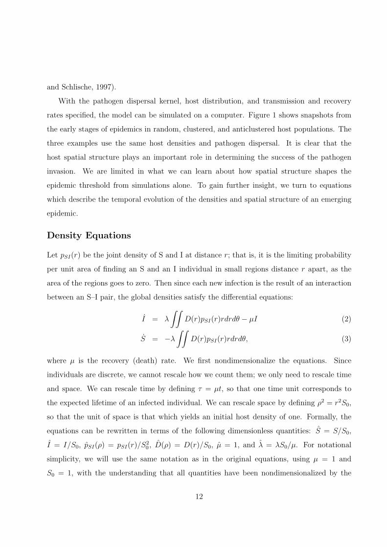
With the pathogen dispersal kernel, host distribution, and transmission and recovery

rates specified, the model can be simulated on a computer. Figure 1 shows snapshots from

the early stages of epidemics in random, clustered, and anticlustered host populations. The

three examples use the same host densities and pathogen dispersal. It is clear that the

host spatial structure plays an important role in determining the success of the pathogen

invasion. We are limited in what we can learn about how spatial structure shapes the

epidemic threshold from simulations alone. To gain further insight, we turn to equations

which describe the temporal evolution of the densities and spatial structure of an emerging

epidemic.

Density Equations

Let pSI(r) be the joint density of S and I at distance r; that is, it is the limiting probability

per unit area of finding an S and an I individual in small regions distance r apart, as the

area of the regions goes to zero. Then since each new infection is the result of an interaction

between an S–I pair, the global densities satisfy the differential equations:

I = λ

∫∫D(r)pSI(r)rdrdθ − µI (2)

S = −λ

∫∫D(r)pSI(r)rdrdθ, (3)

where µ is the recovery (death) rate. We first nondimensionalize the equations. Since

individuals are discrete, we cannot rescale how we count them; we only need to rescale time

and space. We can rescale time by defining τ = µt, so that one time unit corresponds to

the expected lifetime of an infected individual. We can rescale space by defining ρ2 = r2S0,

so that the unit of space is that which yields an initial host density of one. Formally, the

equations can be rewritten in terms of the following dimensionless quantities: S = S/S0,

I = I/S0, pSI(ρ) = pSI(r)/S20 , D(ρ) = D(r)/S0, µ = 1, and λ = λS0/µ. For notational

simplicity, we will use the same notation as in the original equations, using µ = 1 and

S0 = 1, with the understanding that all quantities have been nondimensionalized by the

12

procedure above.

Next, we define the spatial covariance, cSI(r) = pSI(r) − SI, and the scaled covari-

ance, CSI(r) = cSI(r)/SI. Also, we define the weighted scaled covariance by: CSI =∫∫

D(r)CSI(r)rdrdθ. With this notation, the nondimensionalized equations can be written

as:

I = λ(1 + CSI)SI − I (4)

S = −λ(1 + CSI)SI. (5)

When the covariances are zero, spatial structure disappears from the model and we have

the mass action SIR model. Thus, the weighted scaled covariance summarizes the deviation

from the mass action approach; it captures the population structure “seen” from the point

of view of an individual using a given dispersal kernel. This term (CSI) is a clustering index:

when it is positive (negative), the weighted average density of SI pairs is higher (lower) than

would be expected if the individuals were independently distributed. Hereafter, we will refer

to it simply as the covariance.

We can also summarize the spatial structure of the initial host population in terms of

spatial covariances. For a random (Poisson) population, CSS = 0 for all r. For a Poisson

cluster process with density S0 = 1, we have:

CSS(r) = nc(H ∗H)(r), (6)

where H ∗H denotes the convolution of the host dispersal kernel with itself (Diggle, 1983).

Note that the scaled covariance is positive at all distances, and if H(r) decreases monotoni-

cally to zero, then so does the covariance. Finally, the inhibition process yields:

CSS(r) =

−1 r < aγ2 exp(−γU(r))− 1 a < r < 2a0 r > 2a,

(7)

where U(r) = 2πa2− 2a2 cos−1(r/(2a)) + r√

a2 − r2/4 is the area of the union of two circles

of radius a and centers distance r apart (Diggle, 1983). Note that the scaled covariance is

negative up to distance a, after which it is positive and decreases to zero at distance 2a.

13

An epidemic is said to occur if the density of infecteds will increase following an arbitrarily

small introduction: 1I

dIdt

> 0 when S = 1. This yields the threshold criterion: R0 = λ(1 +

CSI) > 1. The question we now face is what value of the dynamic quantity CSI we should

use; as the disease invades, the SI covariance evolves. Since we are computing the threshold

criterion for a successful invasion, we might argue that only the initial behavior of the

model is relevant. When the epidemic is started by randomly infecting host plants, we

could use the initial host covariance for the SI covariance in the main equations. This

approach predicts that the success of the invasion depends only on the host distribution,

and not on the further clustering of infected individuals within the population. Moreover,

for a random host distribution, it predicts that the spatial threshold is the same as the

mass action one, since the host covariance is zero. This approach would be analogous to

incorporating other forms of host heterogeneity, via the coefficient of variation in the host

population (May and Anderson, 1989; Bolker, 1999). However, it does not capture the full

effect of spatial structure on epidemics; the evolution of the SI covariance early in the invasion

is crucial in determining whether or not a true epidemic will occur. Our approach is to use

a pseudoequilibrium value for CSI ; that is, we solve for an equilibrium spatial structure in

the limiting case that S → 1 and I → 0. If the spatial structure of the potential epidemic

develops rapidly, this pseudoequilibrium should capture the effect that spatial structure has

on ability of the disease to invade. Thus, in order to compute the threshold criteria, it is

necessary to understand the dynamics of the spatial covariances.

Moment Closure

The main equations as given above exactly describe the evolution of the mean densities;

however, they include the unknown covariances. In order to arrive at a closed model, we

need to specify the dynamics of the covariances. One approach is to assume that CSI(r) = 0

for all r. This is the so–called mean field assumption, and it yields the nonspatial mass

action model. The mean field model can be seen as the limiting behavior of the spatial

model as dispersal becomes global or in a population of mobile individuals. Alternatively, it

14

can be seen as a first approximation to the behavior of the system with local dispersal. As

Figure 2 shows, the mean field assumption is a poor one when dispersal scales are not large;

it generally overestimates the size of an epidemic. It fails to capture the fact that changing

the pathogen dispersal scale can make the difference between the success and failure of an

epidemic. Finally, the mean field approximation fails to include the effects of the host’s

spatial distribution on the progress of the epidemic.

In order to include spatial structure in the dynamics, we can write down differential

equations for the joint densities:

pSI(|x− y|) = λ

∫

z 6=x

D(|y − z|)pSSI(x, y, z)dz

−λ

∫

z 6=x

D(|y − z|)pISI(x, y, z)dz

−λD(|x− y|)pSI(|x− y|)− pSI(|x− y|) (8)

pSS(|x− y|) = −2λ

∫

z 6=x

D(|y − z|)pSSI(x, y, z)dz (9)

pII(|x− y|) = 2λ

∫

z 6=x

D(|y − z|)pISI(x, y, z)dz

+2λD(|x− y|)pSI(|x− y|)− 2pII(|x− y|). (10)

Here, pSSI(x, y, z) is the joint density of S at x, S at y, and I at z. The derivation of this

equation follows the standard procedure described in Bolker (1999). Essentially, we compute

the dynamics of pairs of sites by following changes to one member of the pair at a time; these

changes may be density independent, due to interaction with the other member, or due to

interactions with a third individual (hence a dependence on “triplet” densities). For example,

the first term in equation 8 describes the creation of an SI pair from the infection of one

member of an SS pair; the second term describes the destruction of an SI pair by infection

of the S by a third plant; the third term describes infection within the pair; the last term

describes the death of the infected plant. These equations are exact, but include the triplet

terms, which are unknown. We arrive at a closed model by assuming that the triplet densities

can be written in terms of mean densities and pairs. This process, known as moment closure,

yields an approximation to the true dynamics that we hope captures the important aspects

15

of spatial structure.

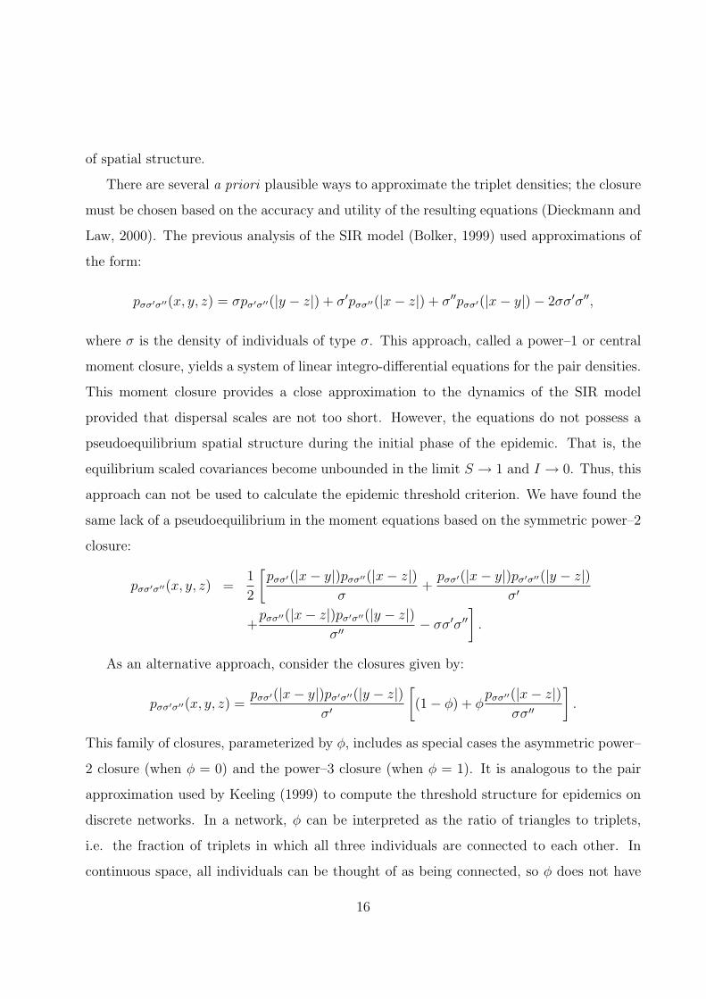
There are several a priori plausible ways to approximate the triplet densities; the closure

must be chosen based on the accuracy and utility of the resulting equations (Dieckmann and

Law, 2000). The previous analysis of the SIR model (Bolker, 1999) used approximations of

the form:

pσσ′σ′′(x, y, z) = σpσ′σ′′(|y − z|) + σ′pσσ′′(|x− z|) + σ′′pσσ′(|x− y|)− 2σσ′σ′′,

where σ is the density of individuals of type σ. This approach, called a power–1 or central

moment closure, yields a system of linear integro-differential equations for the pair densities.

This moment closure provides a close approximation to the dynamics of the SIR model

provided that dispersal scales are not too short. However, the equations do not possess a

pseudoequilibrium spatial structure during the initial phase of the epidemic. That is, the

equilibrium scaled covariances become unbounded in the limit S → 1 and I → 0. Thus, this

approach can not be used to calculate the epidemic threshold criterion. We have found the

same lack of a pseudoequilibrium in the moment equations based on the symmetric power–2

closure:

pσσ′σ′′(x, y, z) =1

2

[pσσ′(|x− y|)pσσ′′(|x− z|)

σ+

pσσ′(|x− y|)pσ′σ′′(|y − z|)σ′

+pσσ′′(|x− z|)pσ′σ′′(|y − z|)

σ′′− σσ′σ′′

].

As an alternative approach, consider the closures given by:

pσσ′σ′′(x, y, z) =pσσ′(|x− y|)pσ′σ′′(|y − z|)

σ′

[(1− φ) + φ

pσσ′′(|x− z|)σσ′′

].

This family of closures, parameterized by φ, includes as special cases the asymmetric power–

2 closure (when φ = 0) and the power–3 closure (when φ = 1). It is analogous to the pair

approximation used by Keeling (1999) to compute the threshold structure for epidemics on

discrete networks. In a network, φ can be interpreted as the ratio of triangles to triplets,

i.e. the fraction of triplets in which all three individuals are connected to each other. In

continuous space, all individuals can be thought of as being connected, so φ does not have

16

a strict interpretation. We use it as a free parameter between 0 and 1, available to tune the

moment equations to match the behavior of the stochastic process. Note that for φ < 1, this

closure is asymmetric: since we are computing the rate of change of state for an individual at

location y, we give more weight to the pairs at locations (x, y) and (y, z) than at (x, z). As

we will show, the moment equations derived from this closure possess a pseudoequilibrium

solution provided that φ is sufficiently small, allowing us to determine the effects of spatial

structure on the epidemic threshold.

Epidemic Dynamics

We begin the analysis by examining how well the moment equations capture the dynamics

of an epidemic. We find it most convenient to express the developing spatial structure in

terms of conditional pair densities: pS|I(r) = pSI(r)/I is the conditional density of S at x

given that there is an I at y. The dynamics of the conditional densities are derived from

the differential equations for the pair densities: pS|I(r) = 1IpSI(r) − pS|I(r) I

I. Covariances

can be recovered from the conditional pair densities: CSI(r) =pS|I(r)

S− 1. Using our closure

scheme in equations 8 – 10 yields the following differential equations for the conditional pair

densities:

pS|I(r) = λ

[(1− φ)pS|S(r)pS|I + φ

pS|S(r)

S(DpS|I ∗ pS|I)(r)− (1− φ)pI|S(r)pS|I

−φpS|I(r)

S(DpS|I ∗ pI|I)(r)−D(r)pS|I(r)− pS|I(r)pS|I

](11)

pI|I(r) = λ

[2(1− φ)pI|S(r)pS|I + 2φ

pS|I(r)S

(DpS|I ∗ pI|I)(r)

+2D(r)pS|I(r)− pI|I(r)pS|I

]− pI|I(r) (12)

pS|S(r) = −λI

SpS|S(r)

[(1− 2φ)pS|I + 2φ

1

S(DpS|I ∗ pS|I)(r)

](13)

By integrating the differential equations for global densities and conditional pair densities,

we obtain solutions that depend on the closure parameter φ. With a Poisson host population

and intermediate pathogen dispersal distance, the moment closure solutions are moderate

17

improvements over the mean field approximation (Figure 3). As the epidemic progresses, the

local buildup of infective individuals leads to a negative covariance between infectives and

susceptibles, slowing the spread of the disease. The covariance dynamics are approximated

best by setting φ = 1 (the power–3 closure). Recall that φ represents the importance of the

relationship between two neighbors of a focal individual. It appears that keeping track of

these relationships is critical for understanding the development of spatial structure in the

epidemic. This may stem from the fact that in the case φ = 0, we can derive: CSS(r) = 0.

That is, the asymmetric power–2 closure predicts that the covariance between susceptible

individuals does not change during the epidemic. In reality, this covariance decreases and

can become negative as gaps form between surviving susceptible plants. Moment closures

with low values of φ fail to capture this thinning of susceptible hosts and underestimate the

magnitude of the negative covariance between infectives and susceptibles.

For sufficiently short pathogen dispersal, the local supply of susceptibles may be com-

pletely exhausted almost immediately; in this case, the epidemic fails to move beyond its

initial foci. The moment equations successfully capture the failure of an epidemic to develop

with short distance pathogen dispersal (Figure 4). Again, the dynamics are best approxi-

mated by setting φ = 1, with lower values underestimating the magnitude of the negative

covariance.

A clustered host population can support a larger epidemic than a randomly distributed

host (Figure 2). The moment equations reproduce this behavior, but they tend to overes-

timate the strength and duration of the positive covariance (Figure 5). The dynamics are

matched best by setting φ = 1, although the rapid oscillations in this solution are qualita-

tively different from the behavior of the stochastic model. Overall, our moment equations

capture the qualitative effects of spatial structure on epidemic dynamics, with the power–3

closure obtained by setting φ = 1 performing best. While they do not handle host clustering

well, they perform better than the power–1 closure (Bolker, 1999) when pathogen dispersal

is over short distance.

18

Threshold Structure

We now return to the problem of computing the epidemic threshold, found by solving the

equation λ(1 + CSI) = 1. For given dispersal and clustering kernels, our goal is to compute

the covariance early in the outbreak and solve for the transmission rate (λ) required for

an epidemic to occur. To determine the relevant covariance, we look for a low density

pseudoequilibrium in the moment equations by setting the dynamics equal to zero. In the

low density limit, we set I = 0, S = 1, and use the host’s original spatial structure for PS|S.

We set PI|S = 0, but we do not assume that PI|I = 0, since the disease may reach nontrivial

levels locally even at low global density. The pseudoequilibrium spatial structure satisfies

the set of equations:

pS|I(r) =(1− φ)pS|S(r)pS|I + φpS|S(r)(DpS|I ∗ pS|I)(r)

D(r) + pS|I + φ(DpS|I ∗ pI|I)(r)(14)

pI|I(r) =1

pS|I(φpS|I(r)(DpS|I ∗ pI|I)(r) + D(r)pS|I(r)) (15)

We cannot solve the equations analytically for the pseudoequilibrium covariance. However,

the equations can be solved numerically as a fixed point problem using the L1 norm. That is,

we plug a trial solution into the right hand side, evaluate, and iterate until the integral of the

difference between the left and right hand sides is as small as we want. From this solution we

calculate the term CSI that we include in the main equations as a parameter. Notice that the

pseudoequilibrium covariance depends only on the spatial parameters of the model; the rate

parameters (µ and λ) affect how quickly the spatial structure develops, but not its form. As

with other moment closures, the pseudoequilibrium equations do not always have bounded

solutions. In particular, the power–3 closure (φ = 1) does not yield a pseudoequilibrium.

More generally, for each set of parameters, there exists a maximum value of φ above which

no pseudoequilibrium solution exists.

The accuracy of the pseudoequilibrium approach can be determined by comparing the

predicted values of R0 with those found in simulations of the stochastic process. In the

simulations, R0 can be estimated from the rate of exponential growth or decline early in

the outbreak: I(t) ≈ I(0) exp((R0 − 1)t). Strictly speaking, an epidemic occurs (R0 > 1)

19

if and only if the number of infected individuals increases after the disease is introduced.

However, in the example of short distance dispersal (Figure 4), the number of infecteds grows

slightly in the simulation before the disease’s spread is checked. However, it does not seem

reasonable to call this an epidemic. In general, the number of infectives may increase while

the spatial structure of the invasion develops; if this spatial structure prevents spreads of

the disease beyond the initial foci, we say that no epidemic has occurred. Thus, we must

choose an appropriate time interval over which to measure the exponential growth or decline

of infecteds in order to estimate R0 from simulations.

Ideally, we would find CSI converging to a pseudoequilibrium early in the outbreak, and

use this to determine the beginning of the time interval for computing R0. However, in simu-

lations the spatial structure continues to evolve on the same time scale as the global spread of

the disease (Figures 3–5); we do not in general find the covariance at a pseudoequilibrium as

the epidemic develops. Thus, we adopt a heuristically motivated approach for estimating R0

from simulations. If the number of infecteds increases or decreases monotonically for more

than one time unit (i.e. the first generation of the disease), we estimate R0 from the initial

phase of the outbreak, on the time interval [0, 1]. When the disease’s spread is checked by

spatial structure developing within the first time unit, we estimate R0 beginning at the peak

in the number of infecteds, typically on the time interval [1, 2]. In the three examples above

(Figures 3–5), the mean field prediction is R0 = 2. The pseudoequilibrium equations with

φ = 0 predict R0 values of 1.90, 0.87, and 2.51. From the simulations, we obtain estimated

R0 values (± standard error) of 1.75± .06, 0.80± .03, and 2.23± .05.

In order to determine the best value of the weighting parameter, φ, for computing the

epidemic threshold, we compared the values of R0 predicted by the moment equations with

values estimated from simulations of the stochastic process over a range of dispersal scales.

For both random and clustered hosts, the best agreement is found with φ = 0, the asym-

metric power–2 closure. As Figure 6 shows, the pseudoequilibrium predictions capture both

the direction and magnitude of deviations from the mean field prediction over a wide range

of spatial scales. Most importantly, there is good agreement between the predicted and

20

simulated epidemic threshold, the parameter combination that yields R0 = 1. Although

closure with φ = 0 underestimates the amount of segregation between susceptible and in-

fected individuals during the epidemic (Figures 3–5), it yields the most reliable threshold

predictions under the pseudoequlibrium approximation. While higher values of φ yield bet-

ter predictions of the development of spatial structure over time, under the approximation

that spatial structure develops instantaneously they overestimate the deviation of R0 from

mean field levels. Thus, our computations of the epidemic threshold structure are based on

the asymmetric power–2 moment closure.

When the initial host density and recovery rate are scaled to 1, the mean field model

predicts that an epidemic will occur if and only if λ > 1. In the spatial SIR model, the

epidemic criterion also involves two spatial factors: the distribution of hosts and dispersal of

pathogens. Under the pseudoequilibrium approximation, an epidemic will occur if and only if

R0 = λ(1+CSI) > 1. Thus, we can compute the epidemic threshold by varying the parameters

governing host distribution and pathogen dispersal, computing the pseudoequilibrium SI

covariance, and solving the invasion criterion for the critical transmission rate λ.

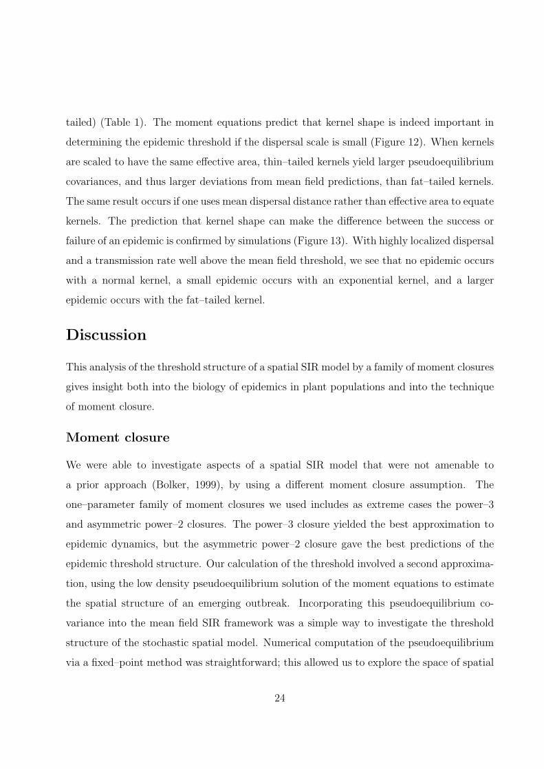
First consider the case of clustered hosts. Figure 7a shows the epidemic threshold when

the pathogen dispersal and host clustering kernels are exponential functions. Where the

threshold surface lies above the plane λ = 1, the moment equations predict that epidemics

require higher transmission than in the mean field system; where the surface is below λ = 1,

spatial structure makes epidemics more likely. When the pathogen dispersal scale is large, the

threshold converges to the mean field case regardless of host distribution, as we would expect.

When the host clustering scale is large, we approach a random distribution (clustering is very

weak). In this limit, the spatial threshold is strictly greater than the mean field threshold;

epidemics are easiest with global pathogen dispersal and become more difficult to achieve as

dispersal decreases.

When the host is clustered, epidemics may be either more or less likely than mean field

theory predicts, depending on the pathogen dispersal scale. Figure 7b shows a typical cross–

section of the threshold surface with constant host clustering. (Each cross–section of the

21

surface has this form, if continued to sufficiently small values of Ad.) As pathogen dispersal

scale decreases from the global case, initially epidemics are more likely to occur. This occurs

because localized dispersal allows the pathogen to take advantage of the local abundance

of susceptible hosts in a clustered distribution. However, if the pathogen dispersal scale

is too short, it quickly depletes the supply of susceptibles even in a clustered population,

preventing a true epidemic. As a result, for any given clustered host population, there is

an intermediate pathogen dispersal scale at which epidemics are the easiest to obtain. The

more tightly clustered the host population, the shorter this optimal dispersal scale will be.

The prediction that for clustered hosts, epidemics are most likely when pathogen dispersal

is intermediate can be confirmed by simulations (Figure 8). Here, the transmission rate is

slightly below 1. For global pathogen transmission, no epidemic occurs. As we decrease

the dispersal scale, we pass through the threshold, and an epidemic occurs, infecting around

8% of the hosts before it runs its course. For extremely short distance pathogen dispersal,

there is an initial burst of infections, but the disease quickly burns out; we have passed back

through the threshold.

For a fixed pathogen dispersal scale, the effect of changing the host clustering is simple.

For any given (finite) Ad, the critical value of λ decreases as Ah decreases. As long as

pathogen dispersal drops off with distance (as in the kernels we employ here), increasing

host proximity makes transmission more likely. Since our dispersal kernels have a maximum

at r = 0, an epidemic would be most likely if all plants occupied the same point in space. This

prediction is also confirmed by simulations (Figure 9). With local pathogen dispersal and

λ = 0.9, we find that no epidemic occurs in the randomly distributed host. As we decrease

Ah so that the host is clustered, we pass through the threshold and obtain epidemics that

increase in size as clustering increases. There is an important caveat regarding the effect

of host clustering on epidemics. Although the threshold transmission rate decreases as host

clustering increases, one cannot assume that the size of the epidemic increases monotonically

with host clustering. Indeed, if hosts are packed into tight groups that are far from one

another, the disease may not spread between clusters. In that case, the final size of the

22

epidemic will be limited by the number of clusters that are initially infected. Thus, tight

clustering may promote the occurence of an epidemic while simultaneously limiting its final

size. Watve and Jog (1997) found that an intermediate cluster size minimized the size of an

epidemic because of this tradeoff between within–cluster and between–cluster spread.

Next, consider the case when hosts are anticlustered; i.e. there is a minimum distance

a between them. When this inhibition distance is 0, we have a randomly distributed host.

As the inhibition distance increases, the moment equations predict that epidemics require

higher transmission (Figure 10). Note that this effect is weak unless Ad is very small,

since over most of the parameter range, the mean pathogen dispersal distance is much

greater than the inhibition distance. For a given initial host density, there is an upper

limit to the inhibition distance we can impose and still achieve the required density; for S0

scaled to 1, the maximum inhibition distance is 1√eπ≈ 0.34. For a fixed host distribution,

the threshold’s dependence on Ad is qualitatively like the randomly distributed case; the

threshold transmission rate is strictly greater than 1 and decreases to 1 as dispersal becomes

global. Simulations support the prediction that epidemics decrease as the inhibition distance

increases (Figure 11), although it is difficult to construct an example in which the host’s

anticlustering clearly moves the system across the epidemic threshold.

Thus far, we have used exponential kernels both for host clustering and pathogen disper-

sal. Next, we consider the effect of changing the shape of the disease dispersal kernel. The

shape of the dispersal kernel has been shown to be important in determining such aspects of

an invasion as the speed and form of a traveling wave (Kot et al., 1996; Lewis and Pacala,

2000), with kernels that decay faster than exponentially (thin–tailed) and kernels that decay

slower than exponentially (fat–tailed) producing qualititatively different results. It is not

clear a priori whether kernel shape will be important in determining the epidemic threshold,

since the pseudoequilibrium covariance may only depend on some measure of the kernel such

as effective area or mean dispersal distance.

To test whether kernel shape does in fact matter, we computed the epidemic threshold for

randomly distributed hosts, using a fat–tailed kernel and the normal kernel (which is thin–

23

tailed) (Table 1). The moment equations predict that kernel shape is indeed important in

determining the epidemic threshold if the dispersal scale is small (Figure 12). When kernels

are scaled to have the same effective area, thin–tailed kernels yield larger pseudoequilibrium

covariances, and thus larger deviations from mean field predictions, than fat–tailed kernels.

The same result occurs if one uses mean dispersal distance rather than effective area to equate

kernels. The prediction that kernel shape can make the difference between the success or

failure of an epidemic is confirmed by simulations (Figure 13). With highly localized dispersal

and a transmission rate well above the mean field threshold, we see that no epidemic occurs

with a normal kernel, a small epidemic occurs with an exponential kernel, and a larger

epidemic occurs with the fat–tailed kernel.

Discussion

This analysis of the threshold structure of a spatial SIR model by a family of moment closures

gives insight both into the biology of epidemics in plant populations and into the technique

of moment closure.

Moment closure

We were able to investigate aspects of a spatial SIR model that were not amenable to

a prior approach (Bolker, 1999), by using a different moment closure assumption. The

one–parameter family of moment closures we used includes as extreme cases the power–3

and asymmetric power–2 closures. The power–3 closure yielded the best approximation to

epidemic dynamics, but the asymmetric power–2 closure gave the best predictions of the

epidemic threshold structure. Our calculation of the threshold involved a second approxima-

tion, using the low density pseudoequilibrium solution of the moment equations to estimate

the spatial structure of an emerging outbreak. Incorporating this pseudoequilibrium co-

variance into the mean field SIR framework was a simple way to investigate the threshold

structure of the stochastic spatial model. Numerical computation of the pseudoequilibrium

via a fixed–point method was straightforward; this allowed us to explore the space of spatial

24

parameters efficiently. The predictions of the pseudoequilibrium approach were confirmed

by simulations; it correctly predicted the effects of the host’s clustering and the disease’s

dispersal scale on R0, and thus on the epidemic threshold.

One could attempt to determine the threshold structure directly by relying only on sim-

ulations rather than the moment equations. However, this approach would be computation-

ally expensive and introduce other difficulties. Since any simulation uses a finite population,

stochasticity can be important in determing the outcome of an invasion. Moreover, criteria

must be established to determine whether or not a given simulation run qualifies as an epi-

demic. This would involve investigating how results scale with the size of the simulation,

and deciding how much of an initial increase in the number of infected inidividuals is allowed

before an epidemic is said to occur. Finally, simulations do not offer explanations for ob-

served phenomena; by contrast, the moment equations allow us to interpret results in terms

of a simple measure of spatial structure during the early phase of an epidemic. By using the

method of moment closure to compute threshold structure, we are sacrificing some accuracy

for efficiency, clarity, and explanatory power.

A possible refinement to our moment closure approach involves tuning the closure as-

sumptions according to the states of the individuals involved. For example, consider the

effect of two infective neighbors on a focal susceptible individual. We could assume that

pISI(x, y, z) = (1 + ε)pIS(|x − y|)pSI(|y − z|)/S for some positive ε. That is, a neighbor

of the susceptible plant is more likely to be infective if another neighbor is infective. This

is analogous to the “improved pair approximation” introduced by Sato et al. (1994), who

found it to be useful for predicting the quantitative and qualitative outcomes of epidemics in

a lattice model. Similarly, Filipe and Gibson (2001) found that a tunable hybrid approach

using both mean field and pair approximations depending on the states involved greatly im-

proved threshold calculations for a lattice model. A similar type of state–dependent moment

closure might improve the threshold predictions in the current model. However, it could

be difficult to compute appropriate tuning parameters in point processes, since they may

depend on the distances between individuals.

25

As Dieckmann and Law (2000) have pointed out, there are a number of plausible moment

closure assumptions that one can make; they advocate a trial and error approach in which one

compares the various moment equations to simulations to determine which version is the most

suitable for a given system. Our study illustrates another aspect to the problem: one must

choose the closure based not just on its accuracy, but on its ability to answer the questions of

interest. For the SIR system, the power 1 closure appears to predict epidemic time series more

accurately than the family of closures used here. On the other hand, our approximations yield

the pseudoequilibrium behavior needed to compute the epidemic threshold. When particular

models are studied intensively using different closure assumptions, we will probably find

not that there is a single best closure, but that the utility of the various versions depends

on the questions being asked, with tradeoffs between accuracy, tractability, explanatory

power, convergence properties, and computational cost. Our analysis clarifies the qualitative

dependence of the epidemic threshold on spatial factors; for detailed predictions of thresholds

or dynamics in a particular population system, one would want to rely on detailed simulation

models rather than the simple one presented here.

Biological insights

Our analysis of a simple spatial SIR model shows that the fundamental question of whether a

disease can cause an epidemic in a sessile population depends not only on the rate of pathogen

production, recovery rate, and host density, but also on the interaction between pathogen

dispersal and host spatial structure. The insight that the epidemic threshold depends on

spatial factors arose in a model that treats hosts as discrete units, rather than a continuous

quantity (as in PDE models). The central result, analogous to lattice model results, is that

local pathogen dispersal tends to cause local saturation of the disease; the spread of the

epidemic is checked if the local (rather than global) supply of susceptible hosts drops below

a critical level. Clustering of hosts increases the local supply of hosts and promotes the

occurence (although not necessarily the size) of epidemics; anticlustering of hosts has the

opposite effect.

26

Our approach to analyzing threshold structure incorporated the spatial structure of an

emerging epidemic into the transmission parameter of the mass action SIR model. This

allowed explicit computation of how the critical transmission rate needed for an epidemic

depends on the details of pathogen dispersal and host distribution. The analysis yielded four

qualitative predictions:

1. When hosts are distributed randomly (Poisson) or are anticlustered, the critical trans-

mission rate increases from the mean field prediction as the pathogen dispersal scale

decreases from infinity.

2. When hosts are clustered, there is an intermediate dispersal scale at which the critical

transmission rate is lowest; longer dispersal fails to take full advantage of locally high

host densities, while shorter dispersal leads to local over–saturation of infectives.

3. For a given pathogen dispersal scale, increasing the degree of host clustering lowers the

critical transmission rate, and increasing the degree of over–dispersal of the host raises

the critical transmission rate.

4. The critical transmission rate depends not only on the mean dispersal distance or effec-

tive area of the pathogen dispersal kernel, but on the kernel’s shape; fat–tailed kernels

lead to less local saturation of infectives and thus have a lower epidemic threshold than

thin–tailed kernels.

While simulations confirm that host clustering promotes the occurence of epidemics, it must

be remembered that this does not necessarily mean that epidemic sizes are also always

increased by clustering. Rather, the inability of the pathogen to travel between distinct

host clusters may limit the final size of the epidemic, even while locally high host densities

promote its early growth (Watve and Jog, 1997).

Further investigation of the dependence of the epidemic threshold on spatial structure is

motivated by several important topics. First, we need to know more about how to control

epidemics in cultivated plants by manipulating the spatial structure of the host population.

27

We have shown that epidemics can be prevented by increasing the scale at which hosts are

clustered, while the overall host density remains the same. More detailed, parameterized

models will be needed to make management recommendations for specific systems. Sec-

ond, epidemic diseases may be important in shaping the spatial structure of natural plant

communities. Locally dispersing pathogens penalize highly clustered populations, and may

contribute to species diversity at both local and regional scales. In order to understand the

role of diseases in structuring plant communities, we need to investigate interactions between

epidemics and other spatially localized processes such as competition. Third, the evolution

of host and pathogen dispersal mechanisms may depend on the interaction between spatial

structure and the epidemic threshold. Selection on pathogen dispersal should favor strains

which exhibit the most rapid growth, i.e. those furthest above the epidemic threshold. Our

analysis indicates that for clustered hosts, there will be an optimal intermediate scale for

pathogen dispersal, while for random or anticlustered hosts, selection will be for long distance

dispersal. The issue for host dispersal is more complicated. While long distance dispersal

will decrease host clustering and thus make epidemics less likely, this may or may not be

selected for. Long distance dispersal decreases the relatedness of neighboring hosts; if there

is strong intraspecific competition, some individuals may benefit from the thinning effect of

an epidemic. Thus, there are likely tradeoffs in the effects of epidemics on the evolution of

host dispersal, depending on the intensity of intraspecific competition and the spatial scale

of resource heterogeneity.

Progress on these issues will require both modeling and experimental approaches. Within

the framework of simple SIR models like the one we analyzed, there are a number of questions

that can be addressed. We should study the effects of dispersal kernels that are qualitatively

different from the ones that we used; advection, vector behavior, and spore aerodynamics

can produce dispersal kernels that are not strictly decreasing with distance from the source.

This may have profound implications for the effect of host distribution on epidemics. In

addition, host spatial distributions will often be more complex than the patterns produced

by the simple clustering and inhibition mechanisms we used. The net effect of positive and

28

negative host correlations at different distances will depend on the dispersal pattern of the

pathogen; for kernels like the ones we used, host distribution at the smallest scale dominates,

but for other types of dispersal, more complex interactions may arise.

There is also a need to extend the simple SIR model to include more details of both hosts

and pathogens, including latent periods, severity of infection, complex pathogen life cycles,

host size structure, and exogenous heterogeneity. Especially important is the heterogeneity

in environmental factors that affect both host and pathogen, such as light and moisture

levels. Local conditions that favor both high host density and rapid pathogen growth may

be critical in determining the spatial structure of epidemics. As epidemic models increase

in complexity, it will be useful to find statistical measures of spatial structure that can be

incorporated in the simple SIR framework, as was the weighted SI covariance in this study.

Finally, it will be important to include vital dynamics of the host in the models in order to

determine how spatial factors affect the conditions for endemicity.

As the theory develops, it will be crucial for the models to be constrained by data from

real systems and to have their predictions tested experimentally. Information on pathogen

dispersal kernels and host spatial distributions in natural systems is needed to parameterize

models. Models tuned to specific systems will then need to have their predictions tested

by experimental manipulation of host distributions and pathogen dispersal. Simple theory

predicts that the occurence of epidemics depends strongly on spatial factors, but we are

only beginning to understand the structure and importance of epidemic thresholds in plant

populations.

Acknowledgments

We thank Alan Hastings and two anonymous reviewers for their thoughtful comments. This

research was conducted with support to D. Brown from NSF DBI-9602226, the Research

Training Grant – Nonlinear Dynamics in Biology, awarded to the University of California,

Davis.

29

References

[1] Ackermann, R.V. and R.W. Schlische (1997). Anticlustering of small normal faults around

larger faults. Geology 25, 1127–1130.

[2] Alexander, H.M. (1989). Spatial heterogeneity and disease in natural plant populations,

in Spatial Components of Plant Disease Epidemics, M.J. Jeger (Ed), Englewood Cliffs:

Prentice Hall.

[3] Anderson, R.M. (1991). Discussion: The Kermack–McKendrick epidemic threshold the-

orem. Bull. Math. Biol. 53, 3–32.

[4] Augspurger, C.K. (1984). Seedling survival of tropical tree species: interactions of dis-

persal distance, light gaps, and pathogens. Ecology 65, 1705–1712.

[5] Aylor, D.E. (1989). Aerial spore dispersal close to a focus of disease. Agr. Forest Meteorol.

47, 109–122.

[6] Bergelson, J., J.A. Newman and E.M. Floresroux (1993). Rates of weed spread in spatially

heterogeneous environments. Ecology 74, 999–1011.

[7] Bohan, D.A., A.C. Bohan, D.M. Glen, W.O.C. Symondson, C.W. Wiltshire and L.

Hughes (2000). Spatial dynamics of predation by carabid beetles on slugs. J. Animal

Ecology 69, 267–379.

[8] Bolker, B.M. (1999). Analytic models for the patchy spread of plant disease. Bull. Math.

Biol. 61, 849–874.

[9] Bolker, B.M. and S.W. Pacala (1997). Using moment equations to understand stochasti-

cally driven spatial pattern formation in ecological systems. Theor. Pop. Biol. 52, 179–197.

[10] Bolker, B.M. and S.W. Pacala (1999). Spatial moment equations for plant competition:

Understanding spatial strategies and the advantages of short dispersal. Am. Nat. 153,

575–602.

30

[11] Brophy, L.S. and C.C. Mundt (1991). Influence of plant spatial patterns on disease

dynamics, plant competition and grain yield in genetically diverse wheat populations.

Agr. Ecosyst. Environ. 35, 1–12.

[12] Burdon, J.J. and G.A. Chilvers (1976). The effect of clumped planting patterns on

epidemics of damping–off disease in cress seedings. Oecologia 23, 17–29.

[13] Carlsson, U. and T. Elmqvist (1992). Epidemiology of anther–smut disease Mi-

crobotryum violaceum and numeric regulation of population of Silene dioica. Oecologia

90, 509–517.

[14] Carlsson, U., T. Elmqvist, A. Wennstrom and L. Ericson (1990). Infection by pathogens

and population age of host plants. J. Ecology 78, 1094–1105.

[15] Cole, B.J., K. Haight and D.C. Wiernasz (2001). Distribution of Myrmecocystus mex-

icanus (Hymenoptera: Formicidae): Association with Pogonomyrmex occidentalis (Hy-

menoptera: Formicidae). Ann. Entomol. Soc. Am. 94, 59–63.

[16] Cressie, N.A.C. (1991). Statistics for Spatial Data, New York: Wiley.

[17] Dale, M.R.T., P. Dixon, M.-J. Fortin, P. Legendre, D.E. Myers and M.S. Rosenberg

(2002). Conceptual and mathematical relationships among methods for spatial analysis.

Ecography 25, 558–577.

[18] Dieckmann, U. and R. Law (2000). Relaxation projections and the method of moments,

in The Geometry of Ecological Interactions: Simplifying Spatial Complexity, U. Dieck-

mann, R. Law, and J. A. J. Metz (Eds), Cambridge: Cambridge Univ. Press.

[19] Diekmann, O. (1978). Thresholds and travelling waves for the geographical spread of

infection. J. Math. Biol. 6, 109–130.

[20] Diekmann, O., J.A.P. Heesterbeek and J.A.J. Metz (1990). On the definition and the

computation of the basic reproduction ratio R0 in models for infectious diseases in het-

erogeneous populations. J. Math. Biol. 28, 365–382.

31

[21] Diggle, P. (1983). Statistical Analysis of Spatial Point Patterns, New York: Academic

Press.

[22] Durrett, R. (1995). Spatial epidemic models, in Epidemic Models: Their Structure and

Relation to Data, D. Mollison (Ed), Cambridge: Cambridge Univ. Press.

[23] Durrett, R. and S.A. Levin (1994). The importance of being discrete (and spatial).

Theor. Popul. Biol. 46, 363–394.

[24] Filipe, J.A.N. and G.J. Gibson (1998). Studying and approximating spatio–temporal

models for epidemic spread and control. Philos. T. Roy. Soc. Lond. B 353, 2153–2162.

[25] Filipe, J.A.N. and G.J. Gibson (2001). Comparing approximations to spatio–temporal

models for epidemics with local spread. Bull. of Math. Biol. 63, 603–624.

[26] Fry, N. (1979). Random point distributions and strain measurement in rocks. Tectono-

physics 60, 89–105.

[27] Gubbins, S., C.A. Gilligan and A. Kleczkowski (2000). Population dynamics of plant–

parasite interactions: Thresholds for invasion. Theor. Popul. Biol. 57, 219–233.

[28] Guttorp, P., D.R. Brillinger and F.P. Schoenberg (2002). Point processes, spatial, in En-

cyclopedia of Environmetrics vol. 3, A.H. El-Shaarawi and W.W. Piegorsch (Eds), Chich-

ester: Wiley and Sons.

[29] Holmes, E. (1997). Basic epidemiological concepts in a spatial context, in Spatial Ecol-

ogy: The Role of Space in Population Dynamics and Interspecific Interactions, D. Tilman

and P. Kareiva (Eds), Princeton: Princeton Univ. Press.

[30] Jeger, M.J. (1986). Asymptotic behaviour and threshold criteria in model plant disease

epidemics. Plant Pathol. 35, 355–361.

[31] Jeger, M.J. (Ed) (1989). Spatial Components of Plant Disease Epidemics, Englewood

Cliffs: Prentice Hall.

32

[32] Jeger, M.J. and F. van den Bosch (1994). Threshold criteria for model plant disease

epidemics. I. Asymptotic results. Phytopathology 84, 24–27.

[33] Keeling, M.J. (1999). The effects of local spatial structure on epidemiological invasions.

P. Roy. Soc. Lond. B 266, 859–867.

[34] Keeling, M.J. and B.T. Grenfell (2000). Individual–based perspectives on R0. J. Theor.

Biol. 203, 51–61.

[35] Kendall, D.G. (1957). Discussion of ‘Measles periodicity and community size’ by M. S.

Bartlett. J. Roy. Stat. Soc. A 120, 48–70.

[36] Kermack, W.O. and A.G. McKendrick (1927). A contribution to the mathematical

theory of epidemics. P. Roy. Soc. Lond. A 115, 700–721.

[37] Kleczkowski, A. and B.T. Grenfell (1999). Mean–field–type equations for spread of epi-

demic: the ‘small world’ model. Physica A 274, 355–360.

[38] Kot, M., M.A. Lewis and P. van den Driessche (1996). Dispersal data and the spread

of invading organisms. Ecology 77, 2027–2042.

[39] Law, R. and U. Dieckmann (2000). Moment approximations of individual–based mod-

els, in The Geometry of Ecological Interactions: Simplifying Spatial Complexity, U. Dieck-

mann, R. Law, and J.A.J. Metz (Eds), Cambridge: Cambridge Univ. Press.

[40] Levin, S.A. and R. Durrett (1996). From individuals to epidemics. Philos. T. Roy. Soc.

Lond. B 351, 1615–1621.

[41] Lewis, M.A. and S. Pacala (2000). Modeling and analysis of stochastic invasion pro-

cesses. J. Math. Biol. 41, 387–429.

[42] Madden, L.V., M.J. Jeger and F. van den Bosch (2000). A theoretical assessment of the

effects of vector–virus transmission on plant virus disease epidemics. Phytopathology 90,

576–594.

33

[43] Matsuda, H., N. Ogita, A. Sasaki and K. Sato (1992). Statistical mechanics of popula-

tion. Prog. Theor. Phys. 88, 1035–1049.

[44] May, R.M. (1990). Population biology and population genetics of plant–pathogen as-

sociations, in Pests, Pathogens and Plant Communities, J.J. Burdon and S.R. Leather

(Eds), Oxford: Blackwell Scientific.

[45] May, R.M. and R.M. Anderson (1989). The transmission dynamics of human immun-

odeficiency virus (HIV), in Applied Mathematical Ecology, S.A. Levin, T.G. Hallam, and

L.J. Gross (Eds), Berlin: Springer–Verlag.

[46] McCallum, H., N. Barlow, and J. Hone (2001). How should pathogen transmission be

modelled? TREE 16, 295–300.

[47] McCartney, H.A. and B.D.L. Fitt (1987). Spore dispersal gradients and disease devel-

opment, in Populations of Plant Pathogens: Their Dynamics and Genetics, M.S. Wolfe

and C.E. Caten (Eds), Oxford: Blackwell Scientific.

[48] McElhany, P., L. Real and A. Power (1995). Vector preference and disease dynamics:

A study of barley yellow dwarf virus. Ecology 76, 444–457.

[49] Metz, J.A.J. and F. van den Bosch (1995). Velocities of epidemic spread, in Epidemic

Models: Their Structure and Relation to Data, D. Mollison (Ed), Cambridge: Cambridge

Univ. Press.

[50] Minogue, K.P. (1989). Diffusion and spatial probability models for disease spread, in

Spatial Components of Plant Disease Epidemics, M.J. Jeger (Ed), Englewood Cliffs: Pren-

tice Hall.

[51] Mundt, C.C. (1989). Modeling disease increase in host mixtures, in Plant Disease Epi-

demiology, vol. II, K.J. Leonard and W. Fry (Eds), New York: McGraw–Hill.

[52] Mundt, C.C. and J.A. Browning (1985). Development of crown rust epidemics in genet-

ically diverse host populations: Effect of genotype unit area. Phytopathology 75, 607–610.

34

[53] Nasell, I. (1995). The threshold concept in deterministic and stochastic models, in Epi-

demic Models: Their Structure and Relation to Data, D. Mollison (Ed), Cambridge: Cam-

bridge Univ. Press.

[54] Onstad, D.W. (1992). Evaluation of epidemiological thresholds and asymptotes with

variable plant densities. Phytopathology 82, 1028–1032.

[55] Ramsay, J.G. and M.I. Huber (1983). The Techniques of Modern Structural Analysis,

vol. 1, London: Academic Press.

[56] Real, L.A. and P. McElhany (1996). Spatial pattern and process in plant–pathogen

interactions. Ecology 77, 1011–1025.

[57] San Jose, J.J., M.R. Farinas and J. Rosales (1991). Spatial patterns of trees and struc-

turing factors in a Trachypogon savanna of the Orinoco Llanos. Biotropica 23, 114–123.

[58] Sato, K., H. Matsuda and A. Sasaki (1994). Pathogen invasion and host extinction in

lattice structured populations. J. Math. Biol. 32, 251–268.

[59] Thieme, H.R. (1977). A model for the spatial spread of an epidemic. J. Math. Biol. 4,

337–351.

[60] Thrall, P.H. and J.J. Burdon (1997). Host–pathogen dynamics in a metapopulation

context: The ecological and evolutionary consequences of being spatial. J. Ecology 85,

743–753.

[61] Thrall, P.H. and J.J. Burdon (1999). The spatial scale of pathogen dispersal: Conse-

quences for disease dynamics and persistence. Evol. Ecol. Res. 1, 681–701.

[62] Watve, M.G. and M.M. Jog (1997). Epidemic diseases and host clustering: An optimum

cluster size ensures maximum survival. J. Theor. Biol. 184, 165–169.

[63] Wright, S. (1946). Isolation by distance under diverse systems of mating. Genetics 31,

39–59.

35

Figure Captions

Table 1: Formulas and summary statistics for pathogen dispersal and host clustering kernels.

Figure 1: Snapshots of simulated epidemics at t = 1. Light gray points are susceptible

plants; black points are infected. Region is 50 x 50, so that the initial plant population is

2500; initially, 1% of plants were infected. Boundaries are periodic. Pathogen transmission

rate is λ = 2 and dispersal is exponential with Ad = 20. (a) Randomly distributed hosts.

(b) Clustered hosts, using exponential kernel with Ah = 12 and nc = 5 plants per cluster.

(c) Anticlustered hosts, with minimum distance a = 0.3 between plants.

Figure 2: Effects of spatial structure on simulated epidemics with the same transmission

rate, λ = 2. Initial density of invectives is 0.005. For the run with clustered hosts, Ah = 5,

with nc = 5 plants per cluster, and Ad = 20. The mean field prediction is the same in all

cases.

Figure 3: Comparison of simulation with moment closure approximations for an epidemic

in a random host population. Transmission rate is λ = 2; disease dispersal scale is Ad = 20.

(a) Density of infectives (starting from 0.005). (b) Weighted scaled SI covariance, CSI .

Figure 4: Comparison of simulation with moment closure approximations for an epidemic

in a random host population. Transmission rate is λ = 2; disease dispersal scale is Ad = 1.

Disease fadeout prevents computing CSI for the full time interval.

Figure 5: Comparison of simulation with moment closure approximations for an epidemic in

a clustered host population. Transmission rate is λ = 2; disease dispersal scale is Ad = 20;

host clustering scale is Ah = 5, with nc = 5 plants per cluster.

Figure 6: Comparison of R0 predicted by the pseudoequilibrium covariance model and esti-

36

mated from simulations (error bars indicate ±1 standard error). Hosts are either randomly

distributed or clustered with Ah = 10 and nc = 5. Transmission rate is λ = 2, so in a

nonspatial epidemic, R0 = 2.

Figure 7: Dependence of epidemic threshold on spatial factors for clustered hosts. Both

host clustering and pathogen dispersal use exponential kernels. (a) Curved surface indicates

critical transmission rate predicted by pseudoequilibrium covariance, as a function of host

clustering scale (Ah) and pathogen dispersal scale (Ad). Plane indicates critical transmis-

sion predicted by mean field model. (b) Cross–section of the threshold surface with Ah = 20.

Figure 8: Effect of dispersal scale on simulated epidemics. Hosts are clustered, with Ah = 5

and nc = 10. “Global” indicates uniform dispersal across the entire region. Finite dis-

persal uses exponential kernel. Transmission rate is λ = 0.8. Estimated values of R0 are:

0.84±0.04 (global, t ∈ [0, 2]); 1.47±0.01 (Ad = 5, t ∈ [0, 1]); 0.86±0.04 (Ad = 0.5, t ∈ [1, 2]).

Figure 9: Effect of clustering scale on simulated epidemics. Hosts are either randomly

distributed or clustered using an exponential kernel and nc = 5. Dispersal is exponential,

with Ad = 10; transmission rate is λ = 0.9. Estimated values of R0 are: 0.82± 0.05 (random

hosts, t ∈ [0, 2]); 1.24± 0.06 (Ah = 5, t ∈ [0, 1]); 1.71± 0.06 (Ad = 1, t ∈ [0, 1]).

Figure 10: Dependence of epidemic threshold on spatial factors for anticlustered hosts.

Pathogen dispersal uses exponential kernel. Curved surface indicates critical transmission

rate predicted by pseudoequilibrium covariance, as a function of minimum distance between

hosts (a) and pathogen dispersal scale (Ad). Plane indicates critical transmission predicted

by mean field model.

Figure 11: Effect of host inhibition distance on simulated epidemics. Hosts are either

randomly distributed or anticlustered using minimum distance between plants a = 0.30.

37

Pathogen dispersal is exponential, with Ad = 10. Transmission rate is λ = 1.6. Estimated

values of R0 are: 1.47± 0.09 (random hosts, t ∈ [0, 1]); 1.42± 0.08 (a = 0.3, t ∈ [0, 1]).

Figure 12: Dependence of epidemic threshold on pathogen dispersal kernel type in a ran-

domly distributed host population. Curves indicate critical transmission rates predicted by

the pseudoequilibrium covariance.

Figure 13: Effect of pathogen dispersal kernel type on simulated epidemics. Hosts are ran-

domly distributed. Dispersal scale is Ad = 1; transmission rate is λ = 4. Estimated values

of R0 are: 0.62 ± 0.11 (normal, t ∈ [0, 1]); 1.85 ± 0.06 (exponential, t ∈ [0, 1]); 1.94 ± 1.94

(fat–tailed, t ∈ [0, 1]).

38

Figures

Table 1:

Name Formula Effective Mean DispersalArea Distance

Exponential m2

2πe−mr 8π

m22m

Normal m2

πe−m2r2 2π

m2

√π

2m

Fat tailed m2

24πe−

√mr 384π

m220m

Figure 1a:

39

Figure 1b:

Figure 1c:

40

Figure 2:

0 5 10 15 20Time

0

0.05

0.1

0.15

Infective

Density

Mean Field

Clustered

Poisson, Ad=20

Poisson, Ad=1

41

Figure 3a:

0 5 10 15 20Time

0

0.05

0.1

0.15

Infective

Density

φ=0

φ=0.5

φ=1

Figure 3b:

0 5 10 15 20Time

0

-0.1

-0.2

-0.3

SICovariance φ=0

φ=0.5

φ=1

42

Figure 4a:

0 2 4 6 8 10 12Time

0

0.0025

0.005

0.0075

0.01

Infective

Density

φ=0φ=0.5

φ=1

Figure 4b:

0 2 4 6 8 10 12Time

0

-0.25

-0.5

-0.75

-1

SI

Covariance

φ=0

φ=0.5

φ=1

43

Figure 5a:

0 2 4 6 8 10 12Time

0

0.1

0.2

0.3

InfectiveDensity

φ=0

φ=0.5

φ=1

Figure 5b:

0 2 4 6 8 10 12Time

-0.5

-0.25

0

0.25

0.5

SI

Covariance φ=0

φ=0.5

φ=1

44

Figure 6:

1 10 100Disease Dispersal Scale, Ad

0.5

1

1.5

2

2.5

R0

Clustered Host

Poisson Host

45

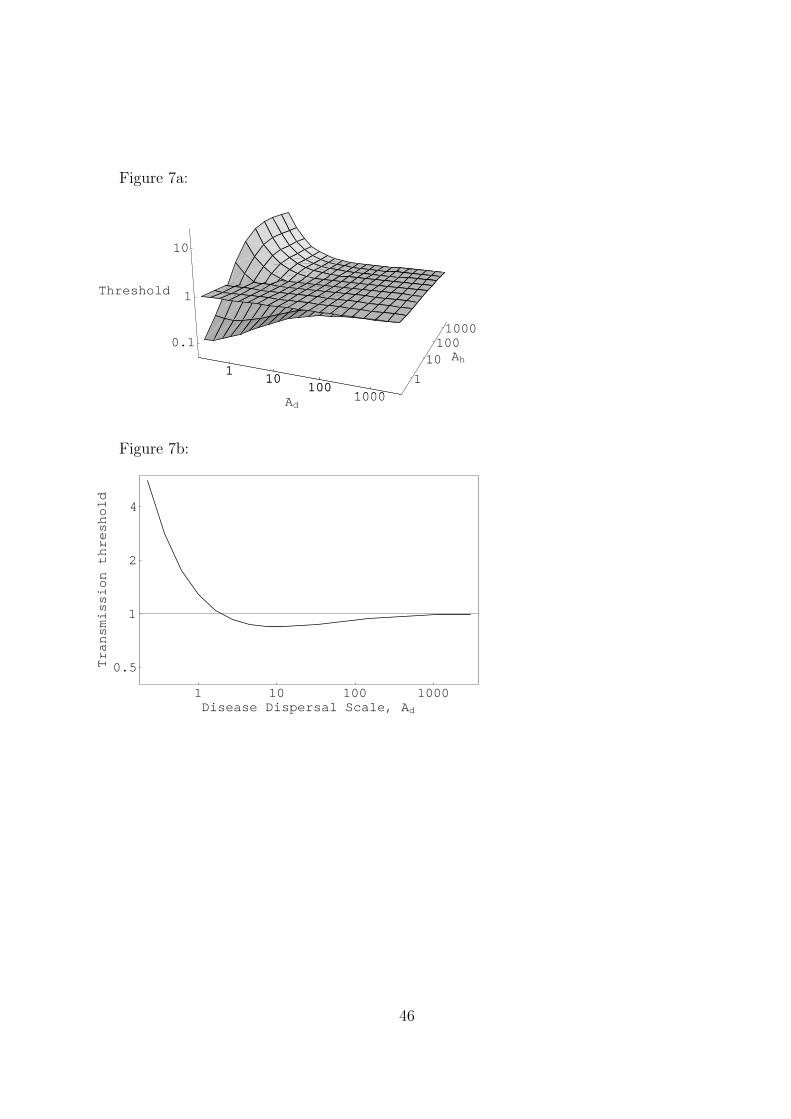
Figure 7a:

110

1001000Ad

1

101001000

Ah0.1

1

10

Threshold

110

1001000Ad

Figure 7b:

1 10 100 1000Disease Dispersal Scale, Ad

0.5

1

2

4

Transmissionthreshold

46

Figure 8:

0 2 4 6 8 10Time

0

0.005

0.01

0.015

InfectiveDensity

Ad=0.5Ad=5Global

Figure 9:

0 2 4 6 8 10Time

0

0.005

0.01

0.015

0.02

InfectiveDensity

Ah=1Ah=5Poisson

47

Figure 10:

110

1001000Ad

0

0.1

0.20.3

a1

2

3

4

5

Threshold

110

1001000Ad

Figure 11:

0 2 4 6 8 10Time

0

0.005

0.01

0.015

Infective

Density

a=0.30

Poisson

48

Figure 12:

1 10 100Disease Dispersal Scale, Ad

1

10

100

Transmissionthreshold

NormalExponentialFat-tailed

Figure 13:

0 2 4 6 8 10Time

0

0.005

0.01

0.015

InfectiveDensity

Fat-tailedExponentialNormal

49