Stochastic Volatility Effects on Defaultable Bonds

Jean-Pierre Fouque∗ Ronnie Sircar† Knut Sølna‡

December 2004; revised October 24, 2005

AbstractWe study the effect of introducing stochastic volatility in the first passage structural approach

to default risk. We analyze the impact of volatility time scales on the yield spread curve. Inparticular we show that the presence of a short time scale in the volatility raises the yield spreadsat short maturities. We argue that combining first passage default modeling with multiscalestochastic volatility produces more realistic yield spreads. Moreover this framework enables usto use perturbation techniques to derive explicit approximations which facilitate the complicatedissue of calibration of parameters.

Contents

1 Introduction 21.1 Defaultable Bonds . . . . . . . . . . . . . . . . . . . . . . . . . . . . . . . . . . . . . 31.2 Outline of the Paper . . . . . . . . . . . . . . . . . . . . . . . . . . . . . . . . . . . . 3

2 The Constant Volatility Case 4

3 Stochastic Volatility 63.1 A Class of Models . . . . . . . . . . . . . . . . . . . . . . . . . . . . . . . . . . . . . 63.2 Stochastic Volatility Effects in Yield Spreads . . . . . . . . . . . . . . . . . . . . . . 8

4 Fast Volatility Factor and Singular Perturbation 124.1 The European Case . . . . . . . . . . . . . . . . . . . . . . . . . . . . . . . . . . . . 124.2 Barrier Options . . . . . . . . . . . . . . . . . . . . . . . . . . . . . . . . . . . . . . . 134.3 Pricing Defaultable Bonds . . . . . . . . . . . . . . . . . . . . . . . . . . . . . . . . . 15∗Department of Mathematics, NC State University, Raleigh NC 27695-8205, fouque@math.ncsu.edu. Work sup-

ported by NSF grant DMS-0455982†Department of Operations Research & Financial Engineering, Princeton University, E-Quad, Princeton, NJ

08544, sircar@princeton.edu. Work partially supported by NSF grants DMS-0306357 and DMS-0456195.‡Department of Mathematics, University of California, Irvine CA 92697, ksolna@math.uci.edu.

1

5 Slow Volatility Factor and Regular Perturbation 16

6 Models with Fast & Slow Volatility Factors 206.1 The Combined Two Scale Stochastic Volatility Models . . . . . . . . . . . . . . . . . 206.2 The Combined Volatility Perturbations . . . . . . . . . . . . . . . . . . . . . . . . . . 226.3 Accuracy of the Approximation . . . . . . . . . . . . . . . . . . . . . . . . . . . . . . 23

6.3.1 Illustration from Numerical Simulations . . . . . . . . . . . . . . . . . . . . . 246.3.2 Convergence Result . . . . . . . . . . . . . . . . . . . . . . . . . . . . . . . . 25

7 Calibration 267.1 Calibration Formulas . . . . . . . . . . . . . . . . . . . . . . . . . . . . . . . . . . . . 267.2 Calibration Exercise . . . . . . . . . . . . . . . . . . . . . . . . . . . . . . . . . . . . 27

A Fast Scale Correction Formulas 31

B Slow Scale Correction Formulas 32

1 Introduction

In this paper, we revisit the first passage structural approach to default. This model supposes thata defaultable zero-coupon bond written on a risky asset X is a bond which pays $1 at maturityT if the asset price Xt stays above a given default threshold B > 0, and pays nothing if Xt goesbelow B at some time before maturity. It is well documented in the literature that in this firstpassage model, yield spreads go to zero with the maturity, which is in contradiction to observeddata. This is illustrated in Figure 1 in the case of highly levered firms, corresponding to X0/Bclose to one. For a general introduction to Credit Risk, including other approaches to default, suchas the intensity based reduced form models, we refer for instance to the books [1], [5], and [22]. Anintroduction can also be found in [16] along with other contributions in the book [23].

As stated by Eom et al. [8], one of the challenges for theoretical pricing models is to raise theaverage predicted spread relative to crude models such as the constant volatility model presentedin the next section, without overstating the risks associated with volatility or leverage. Severalapproaches have been proposed that aim at improving modeling in this regard. These include theintroduction of jumps, [3, 17, 25], stochastic interest rates [20], or imperfect information on X[5, 7]. Another interesting approach is taken in [14] where uncertainty is introduced on the defaultthreshold.

In this paper, we propose to handle this challenge by introducing stochastic volatility in thedynamics of the defaultable asset, and using the framework of multiscale stochastic volatility de-veloped in the context of equity markets [9, 10, 12] and interest-rate derivatives [6].

2

1.1 Defaultable Bonds

Assuming that the underlying is traded, the classical arbitrage free value of a defaultable bond isthe expected value of its discounted payoff computed with respect to a risk neutral measure IP ?,under which the discounted asset price is a martingale. The market may be incomplete and weadopt here the point of view that IP ? is selected by the market among the possible risk neutralpricing measures.

Our focus is on the effect of stochastic volatility, and we study the simplest first-passage model,as introduced by Black-Cox [2] with constant volatility. In the detailed analysis, we assume zerorecovery on default, but we remark on extension to some loss recovery models in Section 2, withthe generalized boundary condition (10). If the risk free interest rate r is constant, the value ofthis bond at time t ≤ T , denoted by ΓB(t, T ), is given by

ΓB(t, T ) = IE?{e−r(T−t)1{inf0≤s≤T Xs>B} | Ft

}(1)

= 1{inf0≤s≤t Xs>B}e−r(T−t)IE?{1{inft≤s≤T Xs>B} | Ft

},

where we denote the expected value with respect to IP ? by IE?, and the history of the dynamicsup to time t by Ft . Indeed ΓB(t, T ) = 0 if the asset price has reached B before time t, whichis reflected by the factor 1{inf0≤s≤t Xs>B}. This defaultable zero-coupon bond is in fact a binarydown-and-out barrier option where the barrier level and the strike price coincide.

Introducing the default time τt defined by τt = inf{s ≥ t,Xs ≤ B}, one has

IE?{1{inft≤s≤T Xs>B} | Ft

}= IP ?{τt > T | Ft},

which shows that the problem reduces to the characterization of the distribution of first-passagetimes. Observe that in the case of a continuous diffusion process Xt, the default time τt is apredictable stopping time, in the sense that it can be announced by an increasing sequence ofstopping times. For instance one can consider the sequence (τ (n)

t ) defined by τ(n)t = inf{s ≥ t,Xs ≤

B + 1/n}. As shown in [15, Theorem 3.1], this implies that yield spreads converge to zero withmaturity. Our approach using stochastic volatility and, in particular, multiscale models, allows toconveniently control the rate of convergence of the spreads, and raise the predicted spreads at shortmaturities.

1.2 Outline of the Paper

In Section 2, we briefly recall the derivation of Merton, and Black and Cox pricing formulas (2)and (8) in the case where the underlying Xt follows a geometric Brownian motion with constantvolatility. This leads to the explicit formula (12) for the yield spreads.

In Section 3, we consider the case where volatility is driven by an additional mean-revertingstochastic factor. In this case, there is no explicit formula for the yield spreads and we study

3

by Monte Carlo simulations the effect of stochastic volatility on the yield spread curve and, inparticular, the effects of volatility time scales. For a long time scale, corresponding to slowlyvarying volatility, we observe a weak effect on long maturities and a negligible effect on shortmaturities. A volatility time scale of order one has an effect comparable to raising the volatilitylevel and does not significantly affect short maturities. However a short time scale, correspondingto fast mean-reverting volatility, produces a significant increase of spreads at short maturities. Wetherefore argue that modeling with a fast stochastic volatility time scale is efficient for handlingthe main challenge of raising spreads at short maturities, while an additional slow scale providesflexibility in capturing long maturity spreads (see Figure 9 for an example).

In Section 4, we carry out a singular perturbation analysis which enables us to obtain the explicitapproximation (34) to the price of a defaultable bond when volatility is fast mean-reverting. Thecase with a slowly mean-reverting stochastic volatility gives rise to a regular perturbation problemwhich we analyze in Section 5. The corresponding explicit price approximation is given in (47).In Section 6, we consider a class of multiscale stochastic volatility models which we analyze bycombining singular and regular perturbation techniques. We show that our explicit formulas for theapproximated prices, involving a few group market parameters, facilitate the essential calibrationstep, which is demonstrated with market data in Section 7.

2 The Constant Volatility Case

We first recall how the price of a defaultable zero-coupon bond is computed in the Black-Scholesmodel

dXt = µXtdt + σXtdWt,

with a constant volatility σ and no dividend. In this case, under the unique risk neutral measureIP ?, the asset price is explicitly given by

Xt = X0 exp(

(r − 12σ2)t + σW ?

t

),

where W ? is a IP ?-Brownian motion.In the Merton [21] approach, default occurs if XT < B for some threshold value B. In this case,

the price at time t of a defaultable bond is simply the price of a European digital option whichpays one if XT exceeds the threshold and zero otherwise. It is explicitly given by ud(t,Xt), where

ud(t, x) = IE?{e−r(T−t)1{XT >B} | Xt = x

}

= e−r(T−t)N(d2(T − t)), (2)

with the distance to default d2 defined by:

d2(T − t) =log

(xB

)+

(r − σ2

2

)(T − t)

σ√

T − t. (3)

4

In the Black and Cox generalization [2], the default occurs the first time the underlying hitsthe threshold B as described in Section 1.1. From a probabilistic point of view, we have

IE?{1{inft≤s≤T Xs>B} | Ft

}

= IP ?

{inf

t≤s≤T

((r − σ2

2)(s− t) + σ(W ?

s −W ?t )

)> log

(B

x

)| Xt = x

},

which can be computed by using the distribution of the minimum of a (non standard) Brownianmotion. From the point of view of partial differential equations, we have

IE?{e−r(T−t)1{inft≤s≤T Xs>B} | Ft

}= uBS(t,Xt; σ),

where uBS(t, x; σ) is the solution of the following problem

LBS(σ)uBS = 0 on x > B, t < T (4)uBS(t, B; σ) = 0 for t ≤ T

uBS(T, x; σ) = 1 for x > B.

Here, LBS(σ) denotes the Black-Scholes partial differential operator at volatility level σ:

LBS(σ) =∂

∂t+

12σ2x2 ∂2

∂x2+ r

(x

∂

∂x− ·

). (5)

This problem can be solved by introducing the solution ud(t, x) of the corresponding digitaloption problem

LBS(σ)ud = 0 on x > 0, t < T (6)ud(T, x) = 1{x>B}.

The price of this European digital option is given by ud(t,Xt) at time t < T , where ud(t, x) iscomputed explicitly in (2). It can be checked that the solution uBS(t, x; σ) of the problem (4) canbe written

uBS(t, x; σ) = ud(t, x)−(

x

B

)1− 2rσ2

ud

(t,

B2

x

). (7)

This formula can be obtained by the method of images presented for instance in [24].We combine the expression (2) for ud(t, x) with (7), to obtain

uBS(t, x; σ) = e−r(T−t)

(N(d+

2 (T − t))−(

x

B

)1− 2rσ2

N(d−2 (T − t))

), (8)

d±2 (T − t) =± log

(xB

)+

(r − σ2

2

)(T − t)

σ√

T − t. (9)

5

Remark: This framework can be adapted for constant or time-dependent deterministic recoveryon default by changing the boundary condition at x = B in equation (4) to

u(t, B; σ) = q(t), (10)

where q is the recovery function. Such non-homogeneous boundary value problems arise in thecomputation of the stochastic volatility correction (see Section 4.2, equation (26)) and we presentthe technique to handle them there. However, we will not explicitly address recovery models here.

Recall that the yield spread Y (0, T ) at time zero is defined by

e−Y (0,T )T =ΓB(0, T )Γ(0, T )

, (11)

where Γ(0, T ) is the default free zero-coupon bond price given here, in the case of constant interestrate r, by Γ(0, T ) = e−rT , and ΓB(0, T ) = uBS(0, x; σ). Notice that the term-structure notationΓB(t, T ) shows the current and maturity times, while the pricing function uBS(t, x;σ) shows thecurrent time, current level of the underlying and the volatility. We thus obtain the formula

Y (0, T ) = − 1T

log

(N

(d+

2 (T ))−

(x

B

)1− 2rσ2

N(d−2 (T )

)). (12)

In Figure 1, we show in the left plot the yield spread curve Y (0, T ) as a function of maturityT for some typical values of the constant volatility, the other parameters are the constant interestrate r and the ratio of initial value to default level x/B. It is well documented in the literaturethat in this first passage model, the likelihood of default is essentially zero for short maturitieseven for highly levered firms, corresponding to B/x close to one, as illustrated in the plots on theright of Figure 1. As discussed in the introduction, the challenge for theoretical pricing models isto raise the average predicted spread relative to crude models such as the constant volatility modelpresented in this section, without overstating the risks associated with volatility or leverage.

In this paper, we propose to handle this challenge by introducing stochastic volatility in thedynamics of the defaultable asset. We explain in the following sections that a naive introduction ofstochastic volatility may not modify the credit spreads significantly. However, a careful modelingof the time scale content of the volatility gives the desired modification in the yield spread at shortmaturities.

3 Stochastic Volatility

3.1 A Class of Models

In the context of equity markets and derivatives pricing and hedging, stochastic volatility is rec-ognized as an essential feature in the modelling of the underlying dynamics. For an extended

6

10−1

100

101

102

0

50

100

150

200

250

300

350

400

450

Time to maturity in years

Yie

ld s

prea

d in

bas

is p

oint

s

10−1

100

101

102

0

50

100

150

200

250

300

350

400

450

Time to maturity in years Y

ield

spr

ead

in b

asis

poi

nts

Figure 1: The plots on the left show the sensitivity of the yield spread curve to the volatility level. Theleverage of the firm B/x is set to 1/1.3, the interest rate r is 6% and the curves increase with the values ofσ: 10%, 11%, 12% and 13%. Note that the time to maturity is in unit of years and plotted on the log scaleand the yield spread is quoted in basis points. The plots on the right show the sensitivity of the yield spreadto the leverage level with the volatility level set to 10%. The curves increases with the increasing leverageratios B/x = (1/1.3, 1/1.275, 1/1.25, 1/1.225, 1/1.2).

discussion, we refer to [9] and the references therein. In order to illustrate our approach we con-sider first the case where volatility is driven by one factor which we assume to be a mean-revertingGaussian diffusion, i.e. an Ornstein-Uhlenbeck process. The dynamics under the physical measureIP is described by the following pair of SDEs

dXt = µXtdt + f1(Yt)Xt dW(0)t , (13)

dYt = α(m− Yt)dt + ν√

2α dW(1)t , (14)

where we assume that

• The volatility function f1 is positive, non-decreasing, and bounded above and away from zero.

• The invariant distribution of the volatility factor Y is the Gaussian distribution with meanm and standard deviation ν and it is independent of the parameter α.

• The important parameter α > 0 is the rate of mean reversion of the process Y . In otherwords 1/α is the time scale of this process, meaning that it reverts to its mean over timesof order 1/α. Small values of α correspond to slow mean reversion and large values of αcorrespond to fast mean reversion.

7

• The standard Brownian motions W (0) and W (1) are correlated as

d⟨W (0),W (1)

⟩t

= ρ1 dt, (15)

where ρ1 is a constant correlation coefficient, with |ρ1| < 1.

We remark that for the purpose of illustration we choose the volatility factor to be an Ornstein-Uhlenbeck process. However, in our approach, Y could be any ergodic diffusion with a uniqueinvariant distribution, as explained in more detail in [9]. Moreover, in our simulations we chooseparticular volatility functions f1(y) as being proportional to max(c1, min(c2, exp(y))), that is theexponential function with lower and upper cutoffs. In Section 5, we use the results of an asymptoticanalysis of this model in the regime with Y being a slowly varying process corresponding to α beingsmall. This requires that f1 is smooth at the current level of the volatility factor y, which is thecase here since cutoffs affect only the tails of f1. In the illustration below, we choose c1 = 0.01 andc2 = 5. These particular choices of Y and f1 are not essential for the perturbation method and theassociated formulas presented in Section 4.

In order to price defaultable bonds under this model for the underlying, we rewrite it under arisk neutral measure IP ? chosen by the market through the market price of volatility risk Λ1:

dXt = rXtdt + f1(Yt)Xt dW(0)?t , (16)

dYt =(α(m− Yt)− ν

√2αΛ1(Yt)

)dt + ν

√2α dW

(1)?t .

Here W (0)? and W (1)? are standard Brownian motions under IP ? correlated as W (0) and W (1). Weassume that the market price of volatility risk Λ1 is bounded and a function of y only.

3.2 Stochastic Volatility Effects in Yield Spreads

In this section, we compute the yield spread that results when we use the stochastic volatility modelin (16). Our focus is the combined role of the mean reversion time 1/α and the correlation ρ1 onthe yield spread curve. We use various values for α, corresponding to volatility factors that rangefrom slowly mean reverting (α = .05) to fast mean reverting (α = 10). For each value of α wepresent a slightly negatively correlated case (ρ1 = −0.05). The effect of a stronger correlation, inaddition to fast mean-reversion, is also shown in Figure 3 (bottom).

In each set of three plots, the top plot gives the yield spread curves as functions of time tomaturity, and the starred curve corresponds to a constant volatility. The solid (higher) curve is theyield curve under the stochastic volatility model (16), where the initial volatility level f1(Y0) andthe long-run average volatility (see (18) below) coincide with the volatility level for the constantvolatility case. The middle plot is analogous, but plotted on a log scale for the time to maturityto resolve the short maturity horizon behavior. The bottom plot shows one realization of thevolatility process f1(Y ) for the corresponding time scale parameters. The constant volatility yieldsare computed using the explicit formula (12). The stochastic volatility yields are computed using

8

Monte Carlo simulations of trajectories for the model (16). For these illustrations we choose thefollowing parameter values: Λ1 = 0, x/B = 1.3, f1(Y0) = 0.12, r = 0.06,m = 0, ν = 0.5.

0 2 4 6 8 10 12 14 16 18 200

100

200

300

Yie

ld s

prea

d in

bas

is p

oint

s

10−1

100

101

102

0

100

200

300

0 2 4 6 8 10 12 14 16 18 200.05

0.1

0.15

0.2

0.25

Time to maturity in years

SV

pat

h

0 2 4 6 8 10 12 14 16 18 200

100

200

300

400

Yie

ld s

prea

d in

bas

is p

oint

s

10−1

100

101

102

0

100

200

300

400

0 2 4 6 8 10 12 14 16 18 200

0.1

0.2

0.3

0.4

Time to maturity in years

SV

pat

h

Figure 2: Correlated (ρ1 = −0.05) mean-reverting stochastic volatility: slowly (α = 0.05) on the left, andorder one (α = 0.5) on the right.

Figure 2 (left) illustrates the effects of a slowly mean reverting volatility with negative correla-tion. The yields for short maturities are not significantly affected. There is a mild spread increasefor longer maturities. (This increase is slightly lower with zero correlation). This feature of thecurve will be captured by analyzing the effect of a slow volatility factor in our model in Section 5.

Figure 2 (right) illustrates the effects of stochastic volatility that runs on the order one timescale. We observe that the effect is similar to an increase in volatility as shown in Figure 1. (Thiseffect is enhanced by negative correlation over the zero correlation case, which is not shown here).This feature of the curve will be captured in the leading order term by choosing an appropriateeffective volatility level σ? in Section 4.3.

Finally, Figure 3 illustrates the effects of a fast mean reverting volatility, with negative corre-lation. In this case, the yields for short maturities are significantly affected with a small negativecorrelation (top row, for different leverage ratios) and even more so with a stronger correlation(bottom graph). It is remarkable that this effect is qualitatively and quantitatively very differentfrom the effect resulting from an increase in the volatility level as shown in Figure 1. This featureof the curve will be captured in our analysis of the stochastic volatility model with a fast meanreverting volatility factor in the following section.

We conclude from these numerical experiments that the time scale content of stochastic volatilityis crucial in the shaping of the yield spread curve. In particular, a short time scale combined witha negative correlation gives enhanced spreads at short maturities, as compared with the constantvolatility case.

9

In Figure 3 (top right), we illustrate the effect of correlated fast mean reverting volatility inthe case of a higher levered bond (x/B = 1.2). We observe that the spread at short maturities aresignificantly higher and again that this effect is qualitatively and quantitatively different from theeffect seen by simply decreasing the level of x/B as seen in Figure 1.

A well separated fast volatility time scale has been observed in equity [10] and fixed income [6]markets. A main feature of this short time scale is that it can be treated by singular perturbationtechniques as described in detail in [9]. This leads to a description where the effects of the stochas-tic volatility can be summarized in terms of two group market parameters, an effective constantvolatility σ? and a skew parameter R3 (which are defined below). Here, we generalize these resultsto the case of defaultable bonds and show how these parameters can be conveniently calibratedfrom the observed yield spread curves. In Section 5, we also introduce a slow volatility time scale,which helps in modeling the yield spread curve at longer maturities.

10

0 2 4 6 8 10 12 14 16 18 200

100

200

300

Yie

ld s

prea

d in

bas

is p

oint

s

10−1

100

101

102

0

100

200

300

0 2 4 6 8 10 12 14 16 18 200

0.2

0.4

0.6

0.8

Time to maturity in years

SV

pat

h

0 2 4 6 8 10 12 14 16 18 200

200

400

600

800

Yie

ld s

prea

d in

bas

is p

oint

s

10−1

100

101

102

0

200

400

600

800

0 2 4 6 8 10 12 14 16 18 200

0.2

0.4

0.6

0.8

Time to maturity in years

SV

pat

h

0 5 10 15 200

200

400

600

Yie

ld s

prea

d in

bas

is p

oint

s

10−1

100

101

102

0

200

400

600

0 5 10 15 200

0.2

0.4

Time to maturity in years

SV

pat

h

Figure 3: Fast mean-reverting (α = 10) stochastic volatility : moderately correlated (ρ1 = −0.05) andmoderately leveraged B/x = 1/1.3 (top left); moderately correlated (ρ1 = −0.05) and more highly leveragedB/x = 1/1.2 (top right); and more strongly correlated (ρ1 = −0.5) and moderately leveraged B/x = 1/1.3(bottom).

11

4 Fast Volatility Factor and Singular Perturbation

In this section, we analyze the effects of a fast mean-reverting volatility factor on defaultablebond prices. Mathematically this involves singular perturbation analysis of barrier options understochastic volatility models (16), in the limit α →∞.

4.1 The European Case

We recall first the singular perturbation results in the case of a European option. Let the payofffunction at the maturity time T be h(x). We denote by PBS(t, x; σ) the Black-Scholes price of thiscontract at time t when the stock price is x and the constant volatility is σ.

The price of the option in the stochastic volatility model (16) is obtained as the expected valueof the discounted payoff under the risk neutral measure :

P (t, x, y) = IE?{e−r(T−t)h(XT ) | Xt = x, Yt = y

}. (17)

In [9] it is shown that in the limit of the volatility time scale going to zero, that is, α → ∞, theprice P converges to the Black-Scholes price computed with an effective constant volatility σ givenby

σ2 =⟨f21

⟩:=

∫f21 (y)Φ(y) dy, (18)

where f21 is averaged with respect to the invariant distribution of the Ornstein-Uhlenbeck process

Φ(y) =1√

2πν2e−(y−m)2/2ν2

.

This limiting price is PBS(t, x; σ), which satisfies the following problem

LBS(σ)PBS = 0 , (19)PBS(T, x) = h(x), (20)

where LBS(σ) is the Black-Scholes operator (5) at the volatility level σ.The main effects of stochastic volatility are captured by the first order correction proportional

to 1/√

α and denoted by P1(t, x). It is given as the solution of the problem

LBS(σ)P1 = −R2x2 ∂2PBS

∂x2−R3x

∂

∂x

(x2 ∂2PBS

∂x2

),

P1(T, x) = 0 ,

where PBS is evaluated at (t, x, σ). The parameters R2 and R3 are small of order√

1/α, and arecomplicated functions of the original model parameters:

R2 =ν√2α〈Λ1φ

′〉, R3 = − ρ1ν√2α〈f1φ

′〉, (21)

12

whereφ′(y) =

1ν2Φ

∫ y

−∞

(f1(u)2 − σ2

)Φ(u) du.

These formulas relating R2, R3 to the original model parameters will not be used explicitly inpractice. In fact we explain in Section 7 how to calibrate directly these parameters from observedyield spreads. In terms of the notation (V2, V3) used in [9], the more convenient notation used hereis related via R2 = 2V3 − V2 and R3 = −V3.

Note that the first order price approximation

P (t, x, y) ≈ PBS(t, x; σ) + P1(t, x)

does not depend on the current level y of the volatility factor which is not directly observed.The calibration is simplified by employing the following alternative approximation, which has

the same order of accuracy. Introducing the corrected effective volatility σ? by

σ?2 = σ2 + 2R2, (22)

the first term in the new approximation is PBS(t, x;σ?). This leads to the correction P ?1 being

defined by

LBS(σ?)P ?1 = −R3x

∂

∂x

(x2 ∂2PBS

∂x2(t, x; σ?)

), (23)

P ?1 (T, x) = 0 ,

so that

P (t, x, y) ≈ PBS(t, x; σ?) + P ?1 (t, x). (24)

The accuracy of this approximation is of order 1/α in the case of a smooth payoff h, and of orderlog(α)/α in the case of call options as proved in [11].

Observe that σ? and R3 are the only parameters needed to compute this approximation, in fact,they can be calibrated from implied volatilities as explained in [13]. In Section 7, we generalize thiscalibration procedure to the case of defaultable bonds.

4.2 Barrier Options

In Section 1.1, we recalled that the price of the defaultable bond is the price of a down and outbarrier digital option. In this section we therefore present the perturbation techniques in the contextof down and out barrier options. See also [18] for fast scale volatility asymptotics for boundaryvalue problems arising from exotic options.

13

Here we consider an option that pays h(XT ) at maturity time T if the the underlying staysabove a level B before time T and zero otherwise. Under the model (16) for the underlying, theprice at time zero of this down and out barrier option is given by

e−rT IE?{h(XT )1{inf0≤s≤T Xs>B}

}.

We define u(t, x, y) by

u(t, x, y) = e−r(T−t)IE?{h(XT )1{inft≤s≤T Xs>B} | Xt = x, Yt = y

},

so that the price of the barrier option at time t is given by

1{inf0≤s≤t Xs>B}u(t,Xt, Yt).

The function u(t, x, y) satisfies for x ≥ B the problem(

∂∂t + LX,Y − r

)u = 0 on x > B, t < T,

u(t, B, y) = 0 for t ≤ T,u(T, x, y) = h(x) for x > B,

where LX,Y is the infinitestimal generator of the process (X, Y ) given by (16).As in the European case, for calibration purposes, it is convenient to construct an asymptotic

approximation in terms of the corrected effective volatility σ? defined in (22). Hence, we defineu?

0(t, x) as the solution of the problem

LBS(σ?)u?0 = 0 on x > B, t < T,

u?0(t, B) = 0 for t ≤ T,

u?0(T, x) = h(x) for x > B,

(25)

and we find the correction u?1(t, x) solves

LBS(σ?)u?1 = −R3 x ∂

∂x

(x2 ∂2u?

0∂x2

)on x > B, t < T,

u?1(t, B) = 0 for t ≤ T,

u?1(T, x) = 0 for x > B.

The derivation follows as in the derivation of (23), with the additional knock-out boundary conditionat x = B. Remarkably, the small parameter R3 is the same as in the European case.

For computing u?1, it is convenient to replace the source problem above by a homogeneous

problem with a non-homogeneous boundary condition. This is achieved by introducing v?1 defined

as

v?1(t, x) = u?

1(t, x)− (T − t)R3 x∂

∂x

(x2 ∂2u?

0

∂x2(t, x)

),

14

so that v?1(t, x) solves the simpler problem

LBS(σ?)v?1 = 0 on x > B, t < T,

v?1(t, B) = g(t) for t ≤ T,

v?1(T, x) = 0 for x > B,

(26)

with the function g(t) given by

g(t) = −R3 (T − t) limx↓B

F3(t, x),

where we define

F3(t, x) = x∂

∂x

(x2 ∂2u?

0

∂x2(t, x)

). (27)

To summarize, we have

u(t, x, y) ≈ u?0(t, x) + (T − t)R3 F3(t, x) + v?

1(t, x) (28)

where u?0 and v?

1 are given in (25) and (26) respectively.

4.3 Pricing Defaultable Bonds

In this section, we consider the case h(x) = 1 corresponding to a defaultable zero coupon bond. Inthis case, u?

0 defined in (25) is explicitly given by

u?0(t, x) = uBS(t, x;σ?), (29)

where uBS was defined in (8)-(9).Calculations for the h = 1 case given in Appendix A lead to the formula

g(t) = R3e−r(T−t)

[1

σ?3

(2√

T − t+ 4pr

√T − t

)N ′(d) + (T − t)(p− 1)p2N(d)

](30)

d = −pσ?√

T − t

2, (31)

wherep = 1− 2r

σ?2 ,

and the formula for F3 defined in (27) is given in equation (56) there.The problem (26) for v?

1 admits the probabilistic representation

v?1(t, x) = IE?{e−r(ξ−t)g(ξ)1{ξ≤T} | X?

t = x > B} (32)

15

where X? is a geometric Brownian motion with volatility σ? and ξ is the first time X? hits theboundary B.

By changing to log coordinates and using a Girsanov transformation, the problem is rewrittenas a first passage problem for a driftless Brownian motion. The distribution of the first hitting timeis known (see for instance [19, Chapter 2]) and v1 can then be written as a Gaussian integral. Weobtain

v?1(t, x) =

(xB

) p2

σ?√

2π

∫ T

t

log(x/B)(s− t)3/2

e− (log(x/B))2

2σ?2(s−t) e−(r+(σ?p)2/8)(s−t)g(s) ds, (33)

where the function g, which is proportional to the small parameter R3, is given in (30).Therefore, the price ΓB(0, T ) of the defaultable bond at time zero, defined in (1), is approxi-

mated by

ΓB(0, T ) ≈ u?0(0, x) + TR3 F3(0, x) + v?

1(0, x) (34)

where u?0(t, x), F3(t, x), and v?

1(t, x) are given in (29), (56), and (33) respectively.In Figure 4, the yield corresponding to this price approximation is represented by the dashed

line, and the yield corresponding to the constant volatility price u?0(t, x) is represented by the solid

line. We use the following values of the parameters σ? = 0.12, r = 0, R3 = −0.0003, x/B = 1.2 andpresent the top plot on a linear scale and the bottom in log maturity coordinates. One sees thatthe correction has qualitatively the shape of the correction seen in Figure 3 (right). The stochasticvolatility strongly affects the yields for short maturities and the effect is very different from thatobtained if only the volatility level is changed. Accuracy of the asymptotic approximation, withrespect to a given, fully specified stochastic volatility model, will be discussed in Section 6.3.

5 Slow Volatility Factor and Regular Perturbation

We have seen in the previous section that the correction generated by the fast mean-revertingstochastic volatility factor affects the yield spreads mainly at short maturities. To gain moreflexibility in calibrating yield spreads we introduce a slow volatility factor which will help the fit atlonger maturities. The importance of this is demonstrated in the calibration in Section 7. In thissection, we summarize the correction generated by a slow volatility factor corresponding to α smallin (16). We denote this factor by Z and its time scale parameter by δ to distinguish from the fastcase analyzed previously. We will combine both fast and slow factors in Section 6.

We rewrite the dynamics of the underlying under the risk neutral measure IP ? as

dXt = rXt dt + f2(Zt)Xt dW(0)?t , (35)

dZt =(δ(m2 − Zt)− ν2

√2δΛ2(Zt)

)dt + ν2

√2δ dW

(2)?t ,

where we assume that

16

0 2 4 6 8 10 12 14 16 18 200

500

1000

1500

2000

2500

Ter

m s

truc

ture

of y

ield

10−1

100

101

0

500

1000

1500

2000

2500

Time to maturity in years

Figure 4: The approximated yield for σ? = 0.12, r = 0.0, R3 = −0.0003, x/B = 1.2. The solid linecorresponds to the constant volatility leading order term. The crossed dashed line incorporates the stochasticvolatility correction. The top plot is on the linear scale and the bottom plot is on the log maturity scale.

• The volatility function f2 is positive, smooth, non-decreasing, bounded above and away fromzero.

• The function Λ2(z) is a market price of volatility risk.

• The small parameter δ > 0 corresponds to the long time scale 1/δ, and the volatility factorZt changes slowly.

• The standard Brownian motions W (0) and W (2) are correlated as

d⟨W (0),W (2)

⟩t

= ρ2 dt, (36)

where ρ2 is a constant correlation coefficient satisfying |ρ2| < 1.

Following [12] and [13], the price of a derivative written on an underlying governed by (35)can be approximated by regular perturbation techniques in the regime δ small. The price of adefaultable bond is given by

ΓB(t, T ) = 1{inf0≤s≤t Xs>B}u(t,Xt, Zt),

17

where u(t, x, z) satisfies the problem(

∂∂t + LX,Z − r

)u = 0 on x > B, t < T,

u(t, B, z) = 0 for t ≤ T,u(T, x, z) = 1 for x > B.

Here, LX,Z is the infinitestimal generator of the process (X, Z) given by (35).The leading order term u

(z)0 (t, x), in the expansion u = u

(z)0 + u

(z)1 + · · ·, solves the problem

LBS(f2(z))u(z)0 = 0 on x > B, t < T,

u(z)0 (t, B) = 0 for t ≤ T,

u(z)0 (T, x) = 1 for x > B,

(37)

where z is only a parameter which corresponds to the current “frozen” level of the slow volatilityfactor. The function u

(z)0 (t, x) is given explicitly by

u(z)0 (t, x) = uBS(t, x; f2(z)),

where uBS was defined in (8)-(9).The first correction u

(z)1 (t, x) solves the problem

LBS(f2(z))u(z)1 = −2

(R0(z)∂uBS

∂σ + R1(z)x ∂∂x

(∂uBS

∂σ

))on x > B, t < T,

u(z)1 (t, B) = 0 for t ≤ T,

u(z)1 (T, x) = 0 for x > B,

(38)

where uBS is evaluated at (t, x, f2(z)), and R0(z) and R1(z) are small parameters of order√

δ,functions of the model parameters:

R0(z) = −√

δ

2ν2Λ2(z)f ′2(z)

R1(z) =

√δ

2ρ2ν2f2(z)f ′2(z),

and depending on the current level z of the slow factor.We again transform this source problem into a homogeneous problem with a non-homogeneous

boundary condition. This is done in three steps. We first introduce

u(z)1a (t, x) = 2(T − t)

(R0(z)

∂uBS

∂σ+ R1(z)x

∂

∂x

(∂uBS

∂σ

)), (39)

18

and then we define

u(z)1b (t, x) = u

(z)1 (t, x)− u

(z)1a (t, x). (40)

Using the relations

LBS(f2(z))(

∂uBS

∂σ

)= −f2(z)x2 ∂2uBS

∂x2,

LBS(f2(z))(

x∂

∂x

(∂uBS

∂σ

))= −f2(z)x

∂

∂x

(x2 ∂2uBS

∂x2

),

we obtain that u(z)1b solves

LBS(f2(z))u(z)1b = 2(T − t)f2(z)

(R0(z)x2 ∂2uBS

∂x2 + R1(z)x ∂∂x

(x2 ∂2uBS

∂x2

))on x > B, t < T,

u(z)1b (t, B) = gb(t) for t ≤ T,

u(z)1b (T, x) = 0 for x > B,

(41)

with

gb(t) = limx↓B

(u

(z)1 (t, x)− u

(z)1a (t, x)

)= − lim

x↓Bu

(z)1a (t, x), (42)

since u(z)1 (t, B) = 0 . Notice that the source term in (41) is now in terms of x-derivatives of uBS .

We are now able to remove the source in (41) by introducing

u(z)1c (t, x) = −(T − t)2f2(z)

(R0(z)x2 ∂2uBS

∂x2+ R1(z)x

∂

∂x

(x2 ∂2uBS

∂x2

)), (43)

and defining

u(z)1d (t, x) = u

(z)1b (t, x)− u

(z)1c (t, x), (44)

which solves

LBS(f2(z))u(z)1d = 0 on x > B, t < T,

u(z)1d (t, B) = gd(t) for t ≤ T,

u(z)1d (T, x) = 0 for x > B,

(45)

with

gd(t) = gb(t)− limx↓B

u(z)1c . (46)

19

To summarize, we have

u(t, x, z) ≈ uBS(t, x; f2(z)) + u(z)1a (t, x) + u

(z)1c (t, x) + u

(z)1d (t, x), (47)

where u(z)1a is given by (39), u

(z)1c is given by (43), and u

(z)1d solves (45).

Equation (45) for u(z)1d , the last contribution to the approximation (47), can be solved by rewrit-

ing it in the log-variable log x, and using distributions for the hitting times of Brownian motionsas in Section 4.3. We obtain

u(z)1d (t, x) =

(xB

) p2

f2(z)√

2π

∫ T

t

log(x/B)(s− t)3/2

exp

(− (log(x/B))2

2f2(z)2(s− t)−

[(f2(z)p)2

8+ r

](s− t)

)gd(s) ds,

(48)where gd(t) is defined in (46), and we have the formula (60) given in Appendix B.

In Figure 5 the yield corresponding to the price approximation (47) is represented by the dashedline, and the yield corresponding to the constant volatility price uBS(t, x; f2(z)) is represented bythe solid line. We use the following values of the parameters f2(z) = 0.12, r = 0.0, R0(z) =0.0003, R1(z) = −0.0005, x/B = 1.2 and present the top plot on a linear scale and the bottom inlog coordinates. One sees that the correction has qualitatively the shape of the correction seenin Figure 2. The stochastic volatility affects the yields for longer maturities with small effects onshort maturities. Accuracy of the asymptotic approximation, with respect to a given, fully specifiedstochastic volatility model, will be discussed in Section 6.3.

6 Models with Fast & Slow Volatility Factors

In this section we consider a class of models which include two stochastic volatility factors withseparated time scales, one fast and the other one slow. We then combine singular and regularperturbations to obtain an approximation for the defaultable bond price. Finally we discuss thecalibration of the parameters needed in this approximation.

6.1 The Combined Two Scale Stochastic Volatility Models

Under the risk-neutral pricing measure IP ?, our model is a combination of (16) and (35) as follows:

dXt = rXtdt + f(Yt, Zt)Xt dW(0)?t , (49)

dYt =

(1ε(m1 − Yt)− ν1

√2√

εΛ1(Yt, Zt)

)dt +

ν1

√2√

εdW

(1)?t ,

dZt =(δ(m2 − Zt)− ν2

√2δ Λ2(Yt, Zt)

)dt + ν2

√2δ dW

(2)?t ,

where we assume that

20

0 2 4 6 8 10 12 14 16 18 200

500

1000

1500

2000

2500

Ter

m s

truc

ture

of y

ield

10−1

100

101

0

500

1000

1500

2000

2500

Time to maturity in years

Figure 5: The approximated yield for f2(z) = 0.12, r = 0.0, R0(z) = 0.0003, R1(z) = −0.0005, x/B = 1.2.The solid line corresponds to the constant volatility leading order term. The dashed line incorporates the slowvarying stochastic volatility correction. The bottom plot is in the log scale and the top plot is in the originalscale.

• The volatility function f(y, z) is positive, smooth in z, non-decreasing, bounded above andaway from zero.

• The functions Λ1(y, z) and Λ2(y, z) are the combined market prices of volatility risk whichdetermine IP ? chosen by the market.

• The short time scale ε and the long time scale 1/δ are such that

ε << 1 <<1δ.

• The standard Brownian motions(W

(0)?t ,W

(1)?t ,W

(2)?t

)are correlated according to the fol-

lowing cross-variations:

d〈W (0)?,W (1)?〉t = ρ1dt,

d〈W (0)?,W (2)?〉t = ρ2dt,

d〈W (1)?,W (2)?〉t = ρ12dt,

where |ρ1| < 1, |ρ2| < 1 and |ρ12| < 1.

21

• The unperturbed volatility process Yt, that is without Λ1, admits the Gaussian invariantdistribution N (m1, ν

21). Averaging with respect to this invariant distribution is again denoted

by 〈·〉.Under this model, the price at time t < T of a zero-coupon defaultable bond maturing at T is givenby

ΓB(t, T ) = 1{inf0≤s≤t Xs>B}u(t,Xt, Yt, Zt),

where u(t, x, y, z) satisfies the problem(

∂∂t + LX,Y,Z − r

)u = 0 on x > B, t < T,

u(t, B, y, z) = 0 for t ≤ T,u(T, x, y, z) = 1 for x > B,

and LX,Y,Z is the infinitestimal generator of the process (X,Y, Z) given by (49). The functionu(t, x, y, z) is approximated in the following section.

6.2 The Combined Volatility Perturbations

Following [12] and [13], one can combine the singular perturbation presented in Section 4, and theregular perturbation presented in Section 5, to obtain:

u(t, x, y, z) = u(z)0 (t, x) + u

(z)1,ε(t, x) + u

(z)1,δ(t, x) + · · · ,

where u(z)0 (t, x) is the order one leading term, u

(z)1,ε(t, x) is proportional to

√ε, u

(z)1,δ(t, x) is propor-

tional to√

δ, and the following terms are of higher order in√

ε and√

δ. The method consistsof expanding first in δ (regular perturbation) and then in ε (singular perturbation), although thereverse order leads to the same approximation. The singular perturbation analysis leads to effectivegroup parameters (σ?, R3) as in Section 4, but these now depend on the “frozen” slow volatilityfactor level z. We obtain group parameters (R0, R1) from the regular perturbation expansion as inSection 5, and these also depend on z.

The function u(z)0 (t, x) is given by (29) where σ? is now z-dependent and denoted by σ?(z). The

function u(z)1,ε(t, x) is given by

u(z)1,ε(t, x) = (T − t)R3(z) F

(z)3 (t, x) + v

?(z)1 (t, x),

where R3(z) is a z-dependent parameter that is small of order√

ε, and F(z)3 (t, x) and v

?(z)1 (t, x) are

given by (56) in Appendix B and (33) respectively, with σ? replaced by σ?(z).As in Section 5, the function u

(z)1,δ(t, x) is the sum of three components

u(z)1,δ(t, x) = u

(z)1a (t, x) + u

(z)1c (t, x) + u

(z)1d (t, x),

22

given respectively by (39), (43) and (48) with f2(z) replaced by σ?(z). In particular, the twoparameters R0 and R1 involved in these components are small of order

√δ and z-dependent.

In terms of the yield spreads Y (0, T ), generated by the full stochastic volatility model (49), weobtain the following approximation

r + Y (0, T ) = − 1T

log(u(0, x, y, z))

≈ − 1T

log(u

(z)0 (0, x) + u

(z)1,ε(0, x) + u

(z)1,δ(0, x)

)

≈ − 1T

log(u

(z)0 (0, x)

)− 1

T

u

(z)1,ε(0, x)

u(z)0 (0, x)

− 1

T

u

(z)1,δ(0, x)

u(z)0 (0, x)

, (50)

where

• The first term is the yield spread produced by the constant volatility model discussed inSection 2, evaluated at the volatility level σ?(z). Therefore σ?(z) is the parameter whichcontrols the yield curve for intermediate maturities (say one to ten years).

• The second term is the correction scaled by the small parameter R3 which affects primarilythe short maturities as shown in Figure 3 (right).

• The third term is the correction scaled by the small parameters R0 and R1 which affect thelonger maturities as shown in Figure 2.

In Figure 6 we show the yield corresponding to the price approximation corresponding to (50)that includes the correction terms from both the fast and the slow scales by the dashed line, and theyield corresponding to the constant volatility price u?

0(t, x) by the solid line. We use the same valuesfor the parameters as above σ? = 0.12, r = 0.0, R0 = 0.0003, R1 = −0.0005, R3 = −0.0003, x/B =1.2. The multiscale stochastic volatility affects the yields significantly for all maturities.

We discuss the error of the approximation (50) in the next section, and in Section 7, we analyzethe form of the correction terms in more detail. In particular we examine how they depend on thegroup market parameters (σ?, R0, R1, R3), that is the parameters we estimate in the calibrationstep.

6.3 Accuracy of the Approximation

We first demonstrate the accuracy of the asymptotic approximation (in the fast mean-revertingcase) with a numerical example, and then provide a precise analytical result for the rate of conver-gence of the complete two-factor (fast and slow) stochastic volatility model.

23

0 2 4 6 8 10 12 14 16 18 200

500

1000

1500

2000

2500

Ter

m s

truc

ture

of y

ield

10−1

100

101

0

500

1000

1500

2000

2500

Time to maturity in years

Figure 6: The approximated yield for σ? = 0.12, r = 0.0, R0 = 0.0003, R1 = −0.0005, R3 = −0.0003, x/B =1.2. The solid line corresponds to the constant volatility leading order term. The dashed line incorporatesthe slow and fast varying stochastic volatility corrections. The bottom plot is in the log scale and the top plotis in the original scale.

6.3.1 Illustration from Numerical Simulations

We consider a fully-specified one-factor fast mean-reverting stochastic volatility model (16) withthe following choices:

r = 0.06, σ = 0.12, ν = 0.5, f1(y) = σe−ν2ey, m = 0,

and with the market price of volatility risk Λ1 ≡ 0. The rate of mean-reversion α varies from 5 to50, corresponding to mean-reversion times from about two months down to about a week.

We compute by Monte Carlo simulations the yield spread (for each α) on a five-year defaultablebond with leverage B/x = 1/1.3. The starting values are X0 = 1, Y0 = 0. We compare withthe approximation given by formula (34), converted to yield spread. The parameters needed inthe approximation (σ?, R3) are related to the original model by formulas (18,21,22) and here arecomputed as σ = 0.12, R3 = −7× 10−5/

√α and σ? = σ since R2 = 0 with our choice Λ1 ≡ 0. For

reference, the corresponding Black-Cox yield, with constant volatility σ, is equal to 2.069%.The following table shows the absolute relative pricing error between the asymptotic approxi-

mation and the true price computed with Monte Carlo (using a cautious 100, 000 paths and 25, 000time-steps per path). Clearly, the error is decreasing as the rate of mean-reversion increases, andthe magnitudes are small.

24

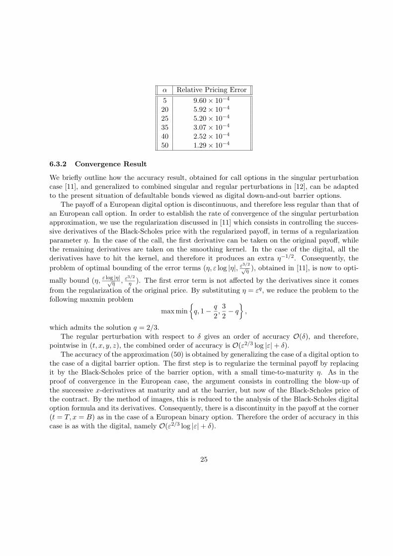
α Relative Pricing Error5 9.60× 10−4

20 5.92× 10−4

25 5.20× 10−4

35 3.07× 10−4

40 2.52× 10−4

50 1.29× 10−4

6.3.2 Convergence Result

We briefly outline how the accuracy result, obtained for call options in the singular perturbationcase [11], and generalized to combined singular and regular perturbations in [12], can be adaptedto the present situation of defaultable bonds viewed as digital down-and-out barrier options.

The payoff of a European digital option is discontinuous, and therefore less regular than that ofan European call option. In order to establish the rate of convergence of the singular perturbationapproximation, we use the regularization discussed in [11] which consists in controlling the succes-sive derivatives of the Black-Scholes price with the regularized payoff, in terms of a regularizationparameter η. In the case of the call, the first derivative can be taken on the original payoff, whilethe remaining derivatives are taken on the smoothing kernel. In the case of the digital, all thederivatives have to hit the kernel, and therefore it produces an extra η−1/2. Consequently, theproblem of optimal bounding of the error terms (η, ε log |η|, ε3/2√

η ), obtained in [11], is now to opti-

mally bound (η, ε log |η|√η , ε3/2

η ). The first error term is not affected by the derivatives since it comesfrom the regularization of the original price. By substituting η = εq, we reduce the problem to thefollowing maxmin problem

maxmin{

q, 1− q

2,32− q

},

which admits the solution q = 2/3.The regular perturbation with respect to δ gives an order of accuracy O(δ), and therefore,

pointwise in (t, x, y, z), the combined order of accuracy is O(ε2/3 log |ε|+ δ).The accuracy of the approximation (50) is obtained by generalizing the case of a digital option to

the case of a digital barrier option. The first step is to regularize the terminal payoff by replacingit by the Black-Scholes price of the barrier option, with a small time-to-maturity η. As in theproof of convergence in the European case, the argument consists in controlling the blow-up ofthe successive x-derivatives at maturity and at the barrier, but now of the Black-Scholes price ofthe contract. By the method of images, this is reduced to the analysis of the Black-Scholes digitaloption formula and its derivatives. Consequently, there is a discontinuity in the payoff at the corner(t = T, x = B) as in the case of a European binary option. Therefore the order of accuracy in thiscase is as with the digital, namely O(ε2/3 log |ε|+ δ).

25

7 Calibration

In this section, we discuss calibration of the asymptotic approximation obtained in the previoussection from yield spread data. The parameters of interest are (σ?, R0, R1, R3). We first reformulatethe approximation in terms of yield, and then illustrate the ability of the model to fit observedyield spread data.

7.1 Calibration Formulas

We rewrite the approximated yield (50) as

Y (0, T ) ≈ Y ?(T ; σ?) + Y ε(T ;σ?) + Y δ(T ;σ?) , (51)

where the leading yield term is given explicitly by

Y ?(T, σ?) = − 1T

log(

N(d+2 )−

(x

B

)p

N(d−2 ))

, (52)

with

p = 1− 2r

σ?, d±2 =

± log(x/B) + pσ?2T/2σ?√

T,

where we do not show the z-dependence in σ?, or in the parameters (R0, R1, R3) below. Themain yield term component Y ? typically captures well the observed yield curves at intermediatematurities. This component is generated by a first passage model with constant volatility σ? whichis therefore the only parameter to be calibrated in this case, if we assumed that the leverage B/xis known.

In this paper we have shown that an extended first passage model with multiscale stochas-tic volatility gives more flexibility to capture the behavior of the yield curve at short and longmaturities. Moreover, by using perturbation techniques we have derived explicit formulas for thecorrections Y ε and Y δ to the yield spread.

The first correction Y ε is given by

Y ε(T ; σ?) = − 1T

(R3 TF3 + v?

1

u?0

), (53)

where u?0, F3, and v?

1 are evaluated at the current time t = 0, current asset value x and maturityT , and given respectively by (29), (56), and (33). Observe from (30) that v?

1 is also proportionalto the small parameter R3 which is fitted in order to capture the yield spread behavior at shortmaturities.

Using the expression (57) for u(z)1a +u

(z)1c given in Appendix B, with f2(z) replaced by σ?(z), the

second correction Y δ is given by

Y δ(T ; σ?) = − 1T

(R0

{2TF0 − T 2σ?F2

}+ R1

{2TF1 − T 2σ?F3

}+ u1d

u?0

), (54)

26

where u?0, F0, F1, F2, F3, and u1d are evaluated at t = 0, current asset value x and maturity T ,

and given respectively by (29), (58), (59), (55), (56), and (48). Observe from (60) that u1d is alsoa sum of terms proportional to either R0 or R1 which are the two small parameters to be fitted inorder to capture the yield spread behavior at longer maturities.

7.2 Calibration Exercise

We demonstrate the versatility of the stochastic volatility models through the approximation for-mulas above, by manually fitting them to some market data. The specific components of the model,namely the base Black-Cox model enhanced with fast and slow stochastic volatility factors, havenatural effects on the yield spreads produced: the base volatility σ? and the leverage B/x enteringthe Black-Cox formula set the basic level of the curve; the fast factor, whose effect is describedthrough the parameter R3, influences the slope of the short end of the curve; and the parametersR0 and R1 associated with the slow factor impact the level and slope respectively of the long end ofthe curve. Of course, the effects of each parameter are not entirely independent, but the physicalinterpretation of their roles makes it natural to employ a visual fitting as a starting point for anautomated procedure. A thorough empirical study with an optimized fitting procedure is beyondthe scope of the current paper.

We take yield spreads from market prices of corporate bonds for two firms, Ford on 9 December2004, when it was rated BBB, and IBM, a firm rated A or higher, on 1 December 2004. The spreadsare obtained from bondpage.com. For simplicity, we assume a constant interest rate r = 0.025throughout.

We first fit the Black-Cox yield spread by varying the volatility σ and the leverage B/x. This isshown by the solid line in Figures 7 and 8. As expected and well-documented, the shape generatedby this model doesn’t capture the data well, especially at shorter maturities. We next exploit theroles of the parameters (R3, R0, R1, R2) in adjusting the yield spread for stochastic volatility. Thisis illustrated in Figure 9 for the Ford data.

The fitted parameters (R0, R1, R2, R3) (reported in the Figure captions) are small, validatingthe use of the asymptotic approximation. Our corrections enable us to match yield spreads formaturities one year and above, compared with only four years and above with the simpler Black-Cox model.

27

0 2 4 6 8 100

1

2

3

4

5

6

7

Time to maturity

Fits to Ford Yields Spreads, 12/9/04

Yie

ld S

prea

ds (

%)

Black−CoxStochastic VolatilityData

Figure 7: Black-Cox and two-factor stochastic volatility fits to Ford yield spread data. The short rate is fixedat r = 0.025. The fitted Black-Cox parameters are σ = 0.35 and x/B = 2.875. The fitted stochastic volatilityparameters are σ? = 0.385, corresponding to R2 = 0.0129, R3 = −0.012, R1 = 0.016 and R0 = −0.008.

0 5 10 15 20 250

1

2

3

4

5

6

Time to maturity (years)

Yie

ld S

prea

d (%

)

Fit to IBM Yield Spreads 12/01/04

Black−CoxStochastic VolatilityData

Figure 8: Black-Cox and two-factor stochastic volatility fits to IBM yield spread data. The short rate is fixedat r = 0.025. The fitted Black-Cox parameters are σ = 0.35 and x/B = 3. The fitted stochastic volatilityparameters are σ? = 0.36, corresponding to R2 = 0.00355, R3 = −0.0112, R1 = 0.013 and R0 = −0.0045.

28

0 5 100

5

10

Add R3

Yie

ld S

prea

ds (

%)

0 5 100

5

10

Add R0

0 5 100

5

10

Time to maturity

Yie

ld S

prea

ds (

%)

Add R1

0 5 100

5

10

Time to maturity

Add R2 ⇒ σ*

Figure 9: The effect of introducing the correction parameters successively. The solid curves in each plotshow the Black-Cox fit to the Ford data with σ = 0.35 and x/B = 2.875. The top left plot shows that the ef-fect of adding the fast factor skew correction parameterized by R3 = −0.012 (with R0 = R1 = R2 = 0)is to get closer to the short maturity yields. Then the level of the curve at longer maturities is ad-justed by bringing in the slow factor level correction parameterized by R0 = −0.008. Next, introducing theslow factor skew correction parameterized by R1 = 0.016 twists the curve to match the slope at medium tolong maturities. Finally, the level of the whole curve is adjusted by R2 (through σ?) as shown in the bottomright plot.

29

References

[1] T. Bielecki and M. Rutkowski. Credit Risk: Modeling, Valuation an Hedging, Springer Finance2002.

[2] F. Black and J.C. Cox. Valuing corporate securities: Some effects of bond indenture provisions.Journal of Finance, 31:351–367, 1976.

[3] S. Boyarchenko. Endogenous Default under Levy Processes. Working paper.

[4] P. Collin-Dufresne and R. Goldstein. Do Credit Spreads Reflect Stationary Leverage Ratios?Reconciling Structural and Reduced Form Frameworks. Journal of Finance 56, 1929-1958,2001.

[5] D. Duffie and K. Singleton. Credit Risk. Princeton University Press, 2003.

[6] P. Cotton, J.P. Fouque, G. Papanicolaou and R. Sircar. Stochastic Volatility Corrections forInterest Rates derivatives, Mathematical Finance 14(2), 173-200, 2004.

[7] D. Duffie and D. Lando. Term Structures of Credit Spreads with Incomplete Accounting In-formation. Econometrica 69, 633-664. 2001.

[8] Y. Eom, J. Helwege, and J.Z. Huang. Structural Models of Corporate Bond Pricing: Anempirical Analysis. Review of Financial Studies 17, 499-544. 2004.

[9] J.-P. Fouque, G. Papanicolaou, and R. Sircar. Derivatives in Financial Markets with StochasticVolatility. Cambridge University Press, 2000.

[10] J.-P. Fouque, G. Papanicolaou, R. Sircar, and K. Sølna. Short Time-Scale in S&P 500 Volatil-ity. Journal of Computational Finance, 6(4): 1–23, 2003.

[11] J.-P. Fouque, G. Papanicolaou, R. Sircar and K. Sølna. Singular Perturbations in OptionPricing. SIAM Journal on Applied Mathematics, 63(5), 1648-1665 (2003).

[12] J.-P. Fouque, G. Papanicolaou, R. Sircar and K. Sølna. Multiscale Stochastic Volatility Asymp-totics. SIAM Journal Multiscale Modeling and Simulation, 2(1): 22-42, 2004.

[13] J.-P. Fouque, G. Papanicolaou, R. Sircar and K. Sølna. Timing the Smile. Wilmott Magazine,March 2004.

[14] K. Giesecke. Correlated default with Incomplete Information. Journal of Banking and Finance,28(7), 1521-1545, 2004.

[15] K. Giesecke. Default and Information. Journal of Economic Dynamics and Control, forthcom-ing, 2005.

30

[16] K. Giesecke. Credit Risk Modelling and Valuation: An Introduction. In Credit Risk, Modelsand Management Ed. D. Shimko, 2nd edition, Risk Books, 487-526, 2004.

[17] B. Hilberink and C. Rogers. Optimal Capital Structure and Endogenous Default, Finance andStochastics, 6(2), 237-263 (2002).

[18] A. Ilhan, M. Jonsson, and R. Sircar, Singular perturbations for boundary value problemsarising from exotic options, SIAM J. Applied Math., 64(4), 1268-1293, 2004.

[19] I. Karatzas and S. Shreve. Brownian Motion and Stochastic Calculus, 2nd edition, Springer-Verlag, 1991.

[20] F. Longstaff and E. Schwartz. Valuing Risky Debt: A New Approach. The Journal of Finance50, 789-821, 1995.

[21] R. Merton. On the pricing of corporate debt: the risk structure of interest rates. Journal ofFinance, 29:449–470, 1974.

[22] Ph. Schonbucher. Credit Derivatives Pricing Models. Wiley, 2003.

[23] D. Shimko (Editor). Credit Risk, Models and Management 2nd edition, Risk Books, 2004.

[24] P. Wilmott, S. Howison, and J. Dewynne. The Mathematics of Financial Derivatives. A studentintroduction. Cambridge University Press, 1995.

[25] C. Zhou. The Term Structure of Credit Spreads with Jump Risk. Journal of Banking andFinance, 25, 2015-2040, 2001.

A Fast Scale Correction Formulas

In this appendix we derive formulas for the function F3(t, x) and g(t) needed in the fast scalecorrection presented in Section 4.3. Using the relations

∂d±2∂x

=±1

xσ√

T − t, N

′′(z) = −zN

′(z) ,

and defining F2(t, x) = x2 ∂2u?0

∂x2 (t, x), one obtains successively

er(T−t)F2(t, x) = N ′(d+2 )

[− d+

2

(σ?√

T − t)2− 1

σ?√

T − t

](55)

+ N ′(d−2 )

[d−2

(σ?√

T − t)2+

2p− 1σ?√

T − t

] (x

B

)p

+ N(d−2 ) [(1− p)p](

x

B

)p

,

31

and

er(T−t)F3(t, x) = N ′(d+2 )

[(d+

2 )2 − 1(σ?

√T − t)3

+d+

2

(σ?√

T − t)2

](56)

+ N ′(d−2 )

[(d−2 )2 − 1

(σ?√

T − t)3+

(3p− 1)d−2(σ?

√T − t)2

+p(3p− 2)σ?√

T − t

] (x

B

)p

+ N(d−2 )[(1− p)p2

] (x

B

)p

.

At the boundary x = B, one has d+2 = d−2 = d defined in (31), and so we deduce formula (30)

for g.

B Slow Scale Correction Formulas

In this appendix we derive formulas for the functions u(z)1a (t, x) + u

(z)1c (t, x) and gd(t) needed in the

slow scale correction presented in Section 5. Observe that

u(z)1a + u

(z)1c = 2(T − t)

(R0F

(z)0 + R1F

(z)1

)− (T − t)2f2(z)

(R0F

(z)2 + R1F

(z)3

), (57)

where F(z)2 and F

(z)3 are given in (55) and (56) with σ? replaced by f2(z), and F

(z)0 and F

(z)1 are

defined by

F(z)0 (t, x) =

∂uBS

∂σ, F

(z)1 (t, x) = x

∂

∂x

(∂u

(z)0

∂σ

),

and given explicitly by

er(T−t)F(z)0 (t, x) = N

′(d+

2 )

[−d+

2

σ−√

T − t

](58)

+ N′(d−2 )

[d−2σ

+√

T − t

] (x

B

)p

+ N(d−2 )[2σ

(p− 1) log(

x

B

)] (x

B

)p

,

er(T−t)F(z)1 (t, x) = N

′(d+

2 )

[(d+

2 )2 − 1σ2√

T − t+

d+2

σ

](59)

+ N′(d−2 )

[(d−2 )2 − 1σ2√

T − t+ (1 + p)

d−2σ

+ p√

T − t +2(1− p)

σ2√

T − tlog

(x

B

)] (x

B

)p

+ N(d−2 )[2σ

(p− 1)(

1 + p log(

x

B

))] (x

B

)p

.

32

At the boundary x = B we have

d+2 = d−2 = d = −pf2(z)

√T − t

2,

and the function gd(t) defined by

gd(t) = − limx↓B

(u

(z)1a (t, x) + u

(z)1c (t, x)

),

is therefore expressed as

gd(t) = −2(T − t)(R0F

(z)0 (t, B) + R1F

(z)1 (t, B)

)+ (T − t)2f2(z)

(R0F

(z)2 (t, B) + R1F

(z)3 (t, B)

).(60)

33