Draft report: Not to be quoted without permission 1

The distribution of household wealth in South Africa using the National Income Dynamics Study – Wave 5

Reza C. Daniels and Safia Khan

1. Introduction This paper follows the fifth wave of the National Income Dynamics Study (NIDS), released in 2018, which includes its third module on wealth since the survey’s inception. The aim of this paper is to investigate nationally representative measures of wealth (household assets, liabilities and net worth) in this most recent NIDS dataset. As wealth is a stock that changes gradually over time, questions on wealth are only included in NIDS every other year the survey is conducted. Previously, NIDS covered the wealth module in its second and fourth waves, conducted in 2010 and 2014/15 respectively. This most recent wave was conducted in 2017/2018. This paper defines wealth as the value of household assets, liabilities and net worth held at the household level in the NIDS sample. As household composition changes over time, this evolution makes longitudinal analysis of the wealth module across survey waves impossible. Instead, the stock of wealth at each point must be analysed cross-sectionally. Nonetheless, this paper presents changes in the measurement of wealth over the last two NIDS waves in which wealth is measured. The wealth instrument used to measure wealth in wave five does not differ from the construct used in wave four (see Daniels & Augustine, 2016). That is, it includes household durable assets in the measure of wealth, and importantly allows for home ownership to be differentiated from land ownership with a land tenure variable identifying private or communal property rights. As with previous NIDS wealth modules, a measure for one shot net worth is present in the dataset, whereby survey respondents are asked what their net worth is inclusive of household possessions. A second “derived” variable for net worth is then constructed as the difference between components of a household’s assets and liabilities. If a substantial subset of these questions are missing, the one-shot net worth variable value is substituted for the derived net worth value. The derived net worth variable is thus a richer measurement of net worth than the one shot net worth measure. Eave wave of the NIDS data was subject to greater levels of attrition, most frequently at the top end of the iCorresponding author: reza.daniels@uct.ac.zancome distribution. In Wave 5, the sample was refreshed with a top-up sample that was specifically targeted to include higher net worth individuals and households (see Nicola Branson’s 2018 Wave 5 paper for a reference). This has created substantively different estimates of household net worth compared to wave 4. The rest of this paper proceeds as follows. Firstly, we evaluate the measurement of household wealth in NIDS wave five. We then evaluate the distribution of assets, liabilities and net worth,

Draft report: Not to be quoted without permission 2

drawing comparisons with previous waves where necessary. Here the impact of the top-up sample on the internal validity of the data is also analysed. The external validity of data is then evaluated using data from the South African Reserve Bank (SARB) on household balance sheets. Household portfolio composition is then discussed. Finally, a discussion on land tenure arrangements and home ownership and its impact on wealth is presented, followed by a conclusion.

2. Measuring Household Wealth in NIDS over time This section briefly discusses how the NIDS wealth instrument is constructed. It should be noted that the instrument used to measure wealth in the NIDS data set changed between the second and the fourth waves, with the change including a new variable for household possessions assets, as well as the separation of land and home ownership (See Daniels & Augustine, 2016). Between waves four and five, the questions have remained the same. The changes between the initial two waves measuring wealth need to be borne in mind when conducting analyses over time using the NIDS. The measure of total assets in wave five is the same as wave four, and is made up of the sum of real estate assets (including houses and other properties), business assets, vehicles, financial assets (which constitute a bank account and stocks), retirement annuities, the value of livestock and household durable assets (or household possessions). The measure of total debt is constructed as the sum of real estate debt (and other properties), business debt, vehicle finance and financial debt (or loans). Then, net worth is defined as the difference between total assets and total debts for each household (for a diagrammatic representation of this, see Daniels and Augustine (2016)). An underestimation of wealth in consumer surveys can be attributed to an under-sampling of wealthy households, which are believed to hold disproportionately higher shares of larger, more valuable assets (Avery, et. al, 1986). A consequence of this is that population estimates based on these assets may be biased downward. In the context of NIDS wave five, a special top-up sample was introduced to enrich the data with a larger number of high income and wealth households.

3. The distribution of assets, liabilities and net worth This section presents an overview of the responses to and measures of wealth in the NIDS wave five sample. It evaluates the responses to the one-shot measure of wealth and compares this measure to the derived measure. It then evaluates the univariate distributions of the components of wealth, looks at inequality measures of the components of wealth and further evaluates the distribution of assets and debts in NIDS wave five.

Draft report: Not to be quoted without permission 3

Table 1: Household level response for one-shot wealth

Frequency Percent Cumulative

Don’t know 2,304 21.6 21.6 Refused 123 1.2 22.7 Missing 10 0.1 22.8 Something left over 5,195 48.6 71.4 Break even 2,678 25.1 96.5 Debt 378 3.5 100 Total 10,688 100

Table 1 above presents the distribution of responses for the one shot wealth question in the wave five dataset. The response shows that just over one fifth of respondents do not know what they would have left over in the event of selling all their assets, whilst just 1.2 percent of respondents refused to answer the question. This refusal rate is similar to the refusal rate in wave four (1.1 percent). The number of respondents who perceive they will have something left over is just less than half (48.6 percent). At the same time a quarter of the sample stated that they would break even. This response should be interpreted carefully because of the bias associated with rounding responses in questionnaires. Surprisingly, only 3.5 percent of households stated that they would be in debt after they sold all their assets. Once again, this number should be interpreted with caution because of the social sensitivity associated with being perceived as being in a financially precarious situation.

The responses presented above are distributed very similarly to the responses from wave four (see: Daniels & Augustine, 2016), boding well for the internal validity of the data and the responses to this question. The second household net worth variable is the derived variable. This is the value of assets less liabilities providing a measure of household net worth that allows one to compare with the one-shot variable. The distribution of both measures of net worth, weighted and unweighted are presented in Table 2 below.

Table 2: Distribution of two measures of household net worth

The table shows the differences between the raw data in the sample and draws a comparison to the weighted data which represents population totals. The first thing to note is the large

Variable Min P10 P25 P50 Mean P75 P95 Max N

Weighted Derived net worth -1 363 544 5 608 20 516

90 850 665 705

377 394 2 450 500 3.44E+08 10,689

One shot net worth -991 460 0 0

15 106 434 482

119 439 1 955 590 7.93E+07 7,932

Unweighted Derived net worth -1 363 544 6 890 24 249

84 340 597 476

288 945 2 048 881 3.44E+08 10,689

One shot net worth -991 460 0 0

15 012 332 196 99 688 1 007 098 7.93E+07 7 933

Draft report: Not to be quoted without permission 4

differences in the unweighted data between one shot net worth and derived net worth, with one shot net worth estimates across percentiles being much lower than derived net worth. This difference is most apparent at the median where derived net worth (which is a more reliable measure) is 5.62 times higher than the estimate from one shot net worth. Similarly, at the higher percentiles of the distribution net worth from the derived estimate is generally much higher than from the one shot estimate. In terms of the weighted estimates, the extremes of the distribution remain unchanged with weights. The bottom of the distribution also remains relatively unchanged, but the impact of the weights is seen from the median upwards for both the derived and one shot measures of net worth. This shows that wealthier households are still under-represented in the data despite the top-up sample. Henceforth, we proceed by only analyzing weighted estimates of the variables. The univariate distributions of the components of wealth are analysed next. Table 3 below the distributions of the components of assets and liabilities. The table alludes to the inequality in the distribution of both assets and debts. This can be seen by looking at the differences between the medians and means of each variable. For instance, the median of total debt in the weighted sample is R7005 whilst the mean is R115 049. This is a mean to median ratio of 16.42, illustrating that the observations at the top end of the debt distribution skew the mean radically. For total assets, the ratio of the mean to median (6.99) is less stark, but still illustrates the extent of the inequality.

Draft report: Not to be quoted without permission 5

Table 3: Distribution of components of assets and liabilities – weighted

Variable Min P10 P25 P50 Mean P75 P95 Max CV N

Total assets 401 9 064 25 642 100 456 702 621 396 811 2 515 425 344 000 000 5.36 10066

Real Estate 1 5 004 24 922 79 750 570 927 344 337 1 982 919 98 300 000 4.39 8192

Business 70 1 301 5 004 25 177 220 426 99 223 983 821 10 000 000 3.00 411

Vehicle 20 24 577 40 284 79 750 133 889 169 192 398 129 8 385 535 1.28 1894

Financial 1 90 300 1 032 52 633 4 359 49 844 344 000 000 64.07 5567

Retirement 55 12 653 43 000 150 061 681 529 496 115 3 021 294 32 500 000 2.99 1048

Livestock 9 420 1 593 13 745 40 944 57 520 154 460 689 064 1.64 676

Possessions 9 4 668 9 969 25 020 98 729 60 047 400 314 24 600 000 5.15 10065

Total debt 2 496 1 856 7 005 115 049 45 268 569 816 17 000 000 4.65 4893

Real Estate 149 59 029 105 904 225 550 548 765 547 428 1 554 438 16 700 000 2.34 517

Business 300 1 991 2 518 6 043 34 392 20 000 99 223 545 727 3.09 29

Vehicle 100 9 869 41 674 90 000 140 667 193 093 467 802 983 064 1.09 551

Financial 2 400 1 496 5 000 23 239 17 314 99 146 2 541 220 3.25 4653

Draft report: Not to be quoted without permission 6

Table 4 presents the Gini coefficients of various financial measures in the data related to wealth from NIDS wave four and wave five. Focusing on the wave five estimates, we see that household income inequality (0.61) is much lower than wealth inequality (0.83) in South Africa. Further inequality for financial assets is exceptionally high, at 0.97, implying an almost completely unequal dispersion of financial assets in the country.

Table 4: Gini coefficients of financial measures

Assets/Debts/Income Gini Wave 4 Gini Wave 5

Total Assets 0.87 0.83 Total Debts 0.90 0.87 Net Worth 0.90 0.83

Household Income 0.61 0.61 Real Estate Assets 0.88 0.83 Retirement Annuities 0.87 0.79

Financial Assets 0.92 0.97 Real Estate Debt - 0.64

Note: The Gini coefficient on net worth was only calculated based on positive (non-zero) values, it is thus not an adequate reflection of inequality in the net worth distribution. Comparing the estimates of Gini coefficients between wave four (2014/15) and wave five (2017/18) we see that on average asset and debt based inequality have declined by four and three percentage points each. Inequality in real estate assets and retirement annuities has also declined. A good measure of the internal validity of this data is reflected in the household income Gini coefficient which remained at 0.61 for both years. Before discussing household portfolio composition, we look at the aggregated components of net worth individually by their respective deciles. Table 5 and Like Table 5, Table 6 shows the median value of debt and share of debt by debt decile. The inequality presented in this figure is also stark, but less so than in the case of assets. The bottom 10 percent of debt holders account for 0.03 percent of total debt, with a median debt value of R66 942. The middle ten percent of the distribution accounts for merely 0.64 percent of total debt with a median debt value of R101 367, this is 1.5 times higher than the median value of debt for the bottom decile. The top decile of debt owners account for a large 76.97 percent of total debt in the country and the median value of debt in this decile is R1 851 596. This is 18.2 times the size of the median debt for the fifth decile and 27.6 times the median value of debt for the bottom decile.

Draft report: Not to be quoted without permission 7

Table 6 present the asset and debt shares by asset and debt decile respectively to provide further insight into the univariate distributions of these variables.

Table 5: Asset shares and value by asset decile

Table 5 shows that the share of assets held by asset decile is considerably unequal in South Africa. The bottom 10 percent of asset holders own 0.07 percent of total assets, with a median value of R5 100. The middle ten percent (the fifth decile) owns only 1.61 percent of total assets with a median value 15.5 times larger than the bottom decile at R78 949. Unsurprisingly, the top decile owns the largest share of assets in the country at 72.7 percent, with a median asset value of R2 534 540, which is 29.8 times the median asset value of the fifth decile and an astounding 461.7 times larger than the median value of assets in the bottom decile. This points to the extent of asset based inequality in South Africa. Further, the median value of assets by asset decile increases almost exponentially at an increasing rate as shown in the figure below.

Figure 1: Median asset value by asset decile

ZAR -

ZAR 500 000

ZAR 1000 000

ZAR 1500 000

ZAR 2000 000

ZAR 2500 000

ZAR 3000 000

1 2 3 4 5 6 7 8 9 10

Median asset value by asset decile

Decile Share (%) Median Value (Rands)

1 0.07 ZAR 5 100 2 0.20 ZAR 13 397 3 0.45 ZAR 25 678 4 0.93 ZAR 49 769 5 1.61 ZAR 78 949 6 2.16 ZAR 122 983 7 3.58 ZAR 202 659 8 5.88 ZAR 396 892 9 12.40 ZAR 852 668 10 72.71 ZAR 2 534 540

Draft report: Not to be quoted without permission 8

Like Table 5, Table 6 shows the median value of debt and share of debt by debt decile. The inequality presented in this figure is also stark, but less so than in the case of assets. The bottom 10 percent of debt holders account for 0.03 percent of total debt, with a median debt value of R66 942. The middle ten percent of the distribution accounts for merely 0.64 percent of total debt with a median debt value of R101 367, this is 1.5 times higher than the median value of debt for the bottom decile. The top decile of debt owners account for a large 76.97 percent of total debt in the country and the median value of debt in this decile is R1 851 596. This is 18.2 times the size of the median debt for the fifth decile and 27.6 times the median value of debt for the bottom decile.

Table 6: Debt shares and value by debt decile

Decile Share Median Value (Rands)

1 0.03 ZAR 66 942

2 0.13 ZAR 69 673

3 0.23 ZAR 71 054

4 0.39 ZAR 108 977

5 0.64 ZAR 101 367

6 1.06 ZAR 124 598

7 1.86 ZAR 170 200

8 5.18 ZAR 303 265

9 13.50 ZAR 756 129

10 76.97 ZAR 1 851 596

The distribution of median debt values by decile is presented in Figure 2 below. As the decile increases, the value of median debt increases at an increasing rate.

Figure 2: Median debt value by debt decile

Draft report: Not to be quoted without permission 9

4. Internal and External validity of the data To analyse the internal validity of the data we start by looking at the change in the components of net worth before the top-up sample was added to the data, and the changes in these components post top-up. Table 7 below shows the minimum, maximum and mean values of each variable. The pre top-up sample was weighted by the weights designed for the initial dataset and the post top-up sample was reweighted taking into account the addition of 1005 new observations of higher income households. The table shows that the addition of the top up sample has increased the mean values of almost all the components of assets and debts, but the extent of this increase varies across variables. The weighted mean value of total assets increased by a factor of 1.1 from R629 886 to R702 621. The mean values of real estate, business and vehicle assets also increased after the top up sample was introduced. The mean value of financial assets decreased from R 53 328 to R52 633 (by 2 percent), indicating that perhaps some wealthier households have less financial assets and more other assets. As expected, the mean values of livestock and possessions did not increase by much with the addition of the new households. What is interesting is that the mean value of retirement annuities decreased from R709 168 to R681 529, this is a decrease of four percent. One potential explanation for this is that the top-up sample may include a higher proportion of individuals already in the retirement stage of the lifecycle implying that the value of their retirement annuities are on average lower. In terms of debts, the mean value of total debt increased by a factor of 1.32 from R87 369 to R115 049, again pointing to the fact that the internal validity of the data is now stronger. Unlike the mean value of assets, where some values decreased, for the components of debt all mean values increased. The largest difference was for business debts, which increased by a factor of 2.97 from R11 570 to R34 392. What this shows is that higher income households

ZAR -

ZAR 200 000

ZAR 400 000

ZAR 600 000

ZAR 800 000

ZAR 1000 000

ZAR 1200 000

ZAR 1400 000

ZAR 1600 000

ZAR 1800 000

ZAR 2000 000

1 2 3 4 5 6 7 8 9 10

Median debt value by debt decile

Draft report: Not to be quoted without permission 10

have a higher values of business debts. The value of real estate debt increase by a factor of 1.25 from R438 955 to R548 765 also indicative of the fact that higher income households have larger values of real estate debt. Overall, however, the increase in mean total asset and debt value post top-up implies that the internal validity of the data is now stronger as higher net worth households were added. This is confirmed by evaluating the mean value of derived net worth, which has increased by a factor of 1.15 from R578 168 to R665 699. Interestingly, the mean value of one shot net worth increased by a factor of 1.55 from R279 798 to R434 482, showing increased trust of higher income households in divulging their financial status to interviewers. This is also an indicator of increased internal validity of the wealth data in NIDS.

Draft report: Not to be quoted without permission 11

Table 7: Comparison of wealth variables before and after top-up sample

Sample without top up – weighted Sample Including top up – weighted

Variable Min Mean Max N Min Mean Max N

Total assets 401 629 886 344 000 000 9 297 401 702 621 344 000 000 10 066

Real Estate 9 487 093 55 500 000 7 529 1 570 927 98 300 000 8 192

Business 70 154 077 10 000 000 350 70 220 426 10 000 000 411

Vehicle 20 120 326 8 385 535 1 362 20 133 889 8 385 535 1 894

Financial 1 53 328 344 000 000 4 939 1 52 633 344 000 000 5 567

Retirement 55 709 168 32 500 000 805 55 681 529 32 500 000 1 048

Livestock 9 40 169 689 064 674 9 40 944 689 064 676

Possessions 9 96 362 14 900 000 9 296 9 98 729 24 600 000 10 065

Total debt 2 87 369 9 919 851 4 439 2 115 049 17 000 000 4 893

Real Estate 149 438 955 9 914 894 282 149 548 765 16 700 000 517

Business 300 11 570 99 688 26 300 34 392 545 727 29

Vehicle 100 135 251 805 678 417 100 140 667 983 064 551

Financial 2 21 957 2 541 220 4 298 2 23 239 2 541 220 4 653

Net worth Derived -964 966 578 168 344 000 000 9 684 -1 363 544 665 699 344 000 000 10 688

Net worth One Shot -500 392 279 798 79 300 000 7 148 -991 460 434 482 79 300 000 7 932

Draft report: Not to be quoted without permission 12

We now turn to the external validity of the data. To determine the external validity of the data we evaluate whether the NIDS estimates of assets and liabilities compare well with estimates from SARB nationally available balance sheets. Since SARB uses tax based data to calculate these figures they are likely to differ substantially from the ones collected using the NIDS instrument. Nonetheless a comparison between the two is drawn below. Table 8: Rand value of components of assets and liabilities in NIDS and SARB

NIDS 2017/18 SARB 2017 NIDS/SARB

Financial Assets 542 000 000 000 8 576 000 000 000 0.06

Non-financial assets 11 600 000 000 000 4 298 000 000 000 2.70

Total assets 12 100 000 000 000 12 874 000 000 000 0.94

Real-estate debt 642 000 000 000 983 000 000 000 0.65

Other debt 363 000 000 000 1 054 000 000 000 0.34

Total debt 1 000 000 000 000 2 036 000 000 000 0.49

Net worth 12 300 000 000 000 10 838 000 000 000 1.13

Source: SARB online statistical query, 2018 Table 8 shows the difference between the values of assets and liabilities between the NIDS and the SARB data. The first interesting finding and the most staggering is the extent to which financial assets are not captured well enough by the NIDS instrument. The table shows that NIDS only captures about 6 percent of the financial asset values reported by SARB. Conversely, NIDS is more efficient at collecting data on non-financial assets, as is shown in row two of the table. It should be borne in mind that non-financial assets include household possessions which are not captured by SARB, so this may be inflating the NIDS estimates, albeit only slightly. Total assets, as captured by NIDS and SARB are quite close in proximity to each other as is net worth. This indicates that the external validity of NIDS regarding assets and net worth, on aggregate, is quite strong. With respect to debt, the external validity of the NIDS instrument is not as strong. The discrepancy between real estate debt, other debt and total debt are all quite large. Recalling Table 1, only 3.5 percent of the sample indicated that they would be in debt in response to the one shot measure of net worth. This is clearly underestimated as is evident from the SARB data and further work needs to go into trying to get respondents to let go of the social sensitivity surrounding perceptions of being “in debt”.

Draft report: Not to be quoted without permission 13

5. Household Portfolio Composition We now turn to household portfolio composition across assets and debts analysed across the asset, debt, net worth, age, income and geolocation distributions. This section provides insight as to the composition of household portfolios across these covariates, allowing an overview of how wealth is distributed in South Africa.

Figure 3: Asset portfolio composition by asset decile

Figure 3 above presents asset portfolio composition by asset deciles. The first thing to note in the figure above is the large share possessions comprise at the bottom deciles of the asset distribution, indicating that households in South Africa, especially at the bottom deciles acquire smaller assets first. Real estate assets are a small share (less than a quarter) in the bottom decile of the asset distribution but this steadily increases to just about half by the fourth decile of the distribution, and to over 50 percent by the fifth decile of the asset distribution in the country. The share of real estate assets remains under 75 percent between the fifth and the tenth percentile, but steadily the share of household possessions as a share of total assets decreases. Retirement annuity assets increase, especially between the seventh and eighth deciles. This shows that at this part of the distribution labour market participation is on the decrease. The share of vehicles as an asset appears noticeably at the fourth decile of the asset distribution but increases substantially in share by the eighth decile of the asset distribution. The eighth, ninth, and tenth deciles have the most significant shares of retirement annuity assets first becoming visible in the sixth decile. Livestock assets are a small share of household assets in south Africa as are business assets, despite the fact that there is a noticeable sliver

Draft report: Not to be quoted without permission 14

of business assets at the top of the South African asset distribution (in the tenth decile). It is important to note that because assets are a stock this distribution has not changed significantly since wave four (See: Daniels & Augustine, 2016).

Figure 4: Debt composition by debt decile

Figure 4 above shows debt composition in South Africa by debt decile. The striking thing about the above figure is that financial debt makes up the largest proportion of debt across all deciles, from one to eight. Vehicle debts make up a very small proportion of overall debt for the third to sixth deciles, and this sliver becomes slightly larger in decile seven. From decile eight onwards the shares of real estate and vehicle debt increase quite substantially. In the eighth, ninth and tenth deciles the share of real estate debt increases steadily, and by the tenth decile real estate debt makes up the largest proportion of debt held. This figure is informative since it shows that the bottom sixty percent of the debt distribution in South Africa have very limited access to vehicle and real estate finance. This changes from the seventh decile, with the eight ninth and tenth having easier access to vehicle and real estate finance. Business debts are a minor component of household debt in South Africa.

Draft report: Not to be quoted without permission 15

Figure 5: Asset portfolio composition by income decile

Draft report: Not to be quoted without permission 16

Figure 5 above now shows the distribution of assets across the income distribution. Income is closely related to wealth, in that those with a higher income have a higher probability of accessing wealth through asset acquisition and access to finance. Ranking income from the smallest ten percent to the top ten percent shows that real estate assets are by far the most common type of assets held by those households who have a labour force income. In fact real estate assets make up more than fifty percent of the asset composition of all the deciles of the income distribution. The second most prominent asset type held is household possessions. With the bottom four deciles’ portfolios comprising at least a quarter of household possessions. Retirement annuities feature slightly in the fifth and sixth deciles of the income distribution but the share increases drastically in from the seventh income decile onwards. The largest share of retirement annuities is held by the top ten percent of income earners. Interestingly, financial assets do not feature prominently except for the ninth decile.

Draft report: Not to be quoted without permission 17

Figure 6: Debt composition by income decile

While financial assets do not feature prominently in the asset distribution across income,

Draft report: Not to be quoted without permission 18

Figure 6 (above) shows that financial debts make up the largest share of debt composition across income decile for the bottom eighty percent of the income distribution in South Africa. Real estate debts increase steadily across the income distribution, comprising more than fifty percent of debts held by the ninth and tenth deciles. The distribution of vehicle debts across income deciles is also interesting – it features as a large share in the bottom ten percent of income earning households then decreases up to the fourth decile, thereafter increasing in share again. Business debts feature only slightly in the composition of debt across income in South Africa.

Draft report: Not to be quoted without permission 19

Figure 7: Asset portfolio composition by household net worth decile

As stated in the discussion above, wealth is a stock, which evolves slowly over time. Figure 8 above shows household asset composition across net worth decile in South Africa providing a snapshot into asset accumulation across the wealth distribution in the country. The patterns observed differ from asset portfolio composition by income, showing that wealth and income, though correlated, result in different behavioural responses by households. An important caveat, before interpreting the above figure, is that because the net worth distribution falls along the negative number line, so that those in the bottom deciles are not necessarily less wealthy than those at the top. In other words, a household with a large number of assets and liabilities may have a net worth of close to zero placing it in a lower decile. Nonetheless, the figure is interesting as it shows that across the net worth distribution the most prominent assets are real estate assets and household possessions. For the second and third deciles household possessions make up more than fifty percent of the share of assets by household net worth. Retirement annuities make up a small share of assets across net worth but considerable shares are seen in in the first, seventh, eighth, ninth and tenth deciles. Once again, why this high proportion of retirement annuities is seen at the bottom of the net worth distribution could be because there are in fact wealthy households in the decile whose assets offset their liabilities. For the latter deciles, the share of household possessions decreases and is replaced by retirement annuities and vehicle assets. Very

Draft report: Not to be quoted without permission 20

interestingly, vehicles make up the largest share of assets for those in the first net worth decile.

Figure 8: Debt composition by household net worth decile

We now turn to debt composition by household net worth decile. Figure 8 (above) shows that for the bottom five deciles, financial debts make up the largest share of debt by net worth decile. Second to this is either real estate debt, or vehicle debts, with the share of these fluctuating between the bottom five deciles. From the seventh to the tenth decile of net worth real estate debts steadily increase in share, with more than three-quarters of real estate debt accounting for the share of debt in the tenth net worth decile. Overall business debts barely feature in the share of household debt by net worth, indicating that households do not seem to take on business debts as part of their portfolios.

Draft report: Not to be quoted without permission 21

Figure 9: Asset portfolio composition by age cohort

Age is an important determinant of the ability to build wealth, as those at the earlier stages of the lifecycle may have constraints to the acquisition of wealth, both assets and liabilities. Figure 9, above, shows the asset portfolios of various age cohorts in South Africa. The first notable thing from the figure is the large proportion of real estate assets across all the age cohorts considered. The share of real estate assets, however, is the highest (over 75 percent) for those above 75, indicating that those closer to the end of the lifecycle have had the ability to acquire much more real estate. For youth, those under the age of 34, and those between 35-44, household possessions make up the second largest share of the household asset portfolio. Financial assets make a prominent appearance for those between the ages of 45-54 indicating that this age cohort is likely saving for retirement, this is in addition to the large share of retirement annuities that this cohort holds. The share of financial assets drops off dramatically from ages 55 and up, also showing that these assets may have become or redeemed as people may switch to other investments. Also worth mentioning is the lack of financial assets and retirement annuities amongst the youth (those under 34), as their inability to save may be hindered by a lack of labour market opportunities, and other lifecycle constraints. Conversely, those between the ages of 35 and 75 have a relatively large share of retirement annuities, indicative of the saving phase of the lifecycle. We now turn to debt composition by age cohort. Figure 10 shows the debt composition by age cohort and some interesting trends emerge. The first is that for those under 24 the largest share of their debt portfolio comprises financial debt, this could be inclusive of student loans,

Draft report: Not to be quoted without permission 22

general credit and overdraft facilities. The second largest debt category for this age group is vehicle debt, as vehicular finance may be relatively easier to access compared to other debt for this age group. Real estate debt makes up the smallest share of debt for this age cohort. As age increases, along with the lifecycle pattern of consumption real estate debt begins to increase as households acquire property. By the ages 55-64 real estate debt makes up about three quarters of the debt portfolio. However, this share declines from ages 65 and up as the debt is steadily paid off as the lifecycle progresses. For those in retirement, that is, those above 75, financial debts make up the largest share of the household debt portfolio. While this seems similar to the breakdown of debt for those under 24, it is important to recall that the figure only represents shares of debt and not actual debt amounts.

Figure 10: Debt composition by age cohort

Access to wealth can be constrained by geo-location, this is particularly the case for debt where access to financial institutions can be limited. Similarly, asset acquisition may be hindered by a lack of labour market opportunity based on the location of a household. This section now turns to asset and debt portfolio composition by geo-location. There are four classifications in the NIDS data that are considered here. Namely, rural formal areas, urban formal areas, urban informal areas and tribal authority areas (or chiefdoms). Figure 11 below shows asset portfolio allocation by geotype. A good starting point is the urban formal categorization. This group of households comprise an asset portfolio made up mostly of real estate assets (more than fifty percent). This is followed by retirement annuities, indicating their close proximity to urban labour markets. The next category that makes up a large share of urban formal household asset portfolios is household posessions, with a smaller share of financial assets and a very small share of business assets.

Draft report: Not to be quoted without permission 23

Compared to this group, urban informal household asset portfolios comprise of slightly less than fifty percent real-estate. The second largest share is made up of household possessions, indicating a substitution effect of land for possessions as possessions may be easier to acquire. Retirement annuities rank third for those in urban informal areas, with a smaller share then was presented for urban formal household asset portfolios. Vehicle assets follows retirement annuities for the urban informal category. Most interesting, vis-à-vis urban formal households is the larger share of business assets in this category indicative of a potentially larger pool of self-employed households in urban informal settings. On this note, there seems to be a trade-off of financial assets for business assets for this group, as financial assets make up the smallest share of urban informal household asset portfolios.

Figure 11: Asset portfolio composition by geotype

Figure 11 also shows the asset composition of rural formal and tribal authority areas. As with urban formal households, households in these two categories also present real estate assets as the largest share of their asset portfolios (both slightly over fifty percent). For rural formal households, possessions make up the second largest share of household assets. In fact across all four location categories, the share for possessions as a share of the asset portfolio is largest in rural formal areas. As alluded to earlier, this could be due to the ease of access with which household possessions can be acquired. Tribal authority areas also present a relatively high share of household possessions compared to urban formal households. Whilst retirement annuities make up the third largest share of assets in tribal authority areas they make up only a small share of assets in rural formal areas. Finally, livestock assets make up a noticeable share of assets in tribal authority areas, and a tiny proportion of assets in rural formal areas but do not feature in the asset compositions of urban formal and urban informal areas.

Draft report: Not to be quoted without permission 24

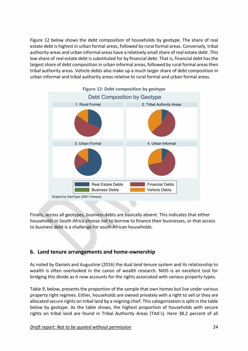
Figure 12 below shows the debt composition of households by geotype. The share of real estate debt is highest in urban formal areas, followed by rural formal areas. Conversely, tribal authority areas and urban informal areas have a relatively small share of real estate debt. This low share of real estate debt is substituted for by financial debt. That is, financial debt has the largest share of debt composition in urban informal areas, followed by rural formal areas then tribal authority areas. Vehicle debts also make up a much larger share of debt composition in urban informal and tribal authority areas relative to rural formal and urban formal areas.

Figure 12: Debt composition by geotype

Finally, across all geotypes, business debts are basically absent. This indicates that either households in South Africa choose not to borrow to finance their businesses, or that access to business debt is a challenge for south African households.

6. Land tenure arrangements and home-ownership As noted by Daniels and Augustine (2016) the dual land tenure system and its relationship to wealth is often overlooked in the canon of wealth research. NIDS is an excellent tool for bridging this divide as it now accounts for the rights associated with various property types. Table 9, below, presents the proportion of the sample that own homes but live under various property right regimes. Either, households are owned privately with a right to sell or they are allocated secure rights on tribal land by a reigning chief. This categorization is split in the table below by geotype. As the table shows, the highest proportion of households with secure rights on tribal land are found in Tribal Authority Areas (TAA’s). Here 38.2 percent of all

Draft report: Not to be quoted without permission 25

households in these areas are allocated secure rights. Second to this, secure rights are also found in smaller proportions in rural formal areas, where about one in ten (9.9 percent) of households in these possess these secure rights through tribal land allocation. The proportion of households with secure rights on tribal land is much smaller in urban formal and urban informal locations, with 1.6 percent and 4.5 percent of households possessing secure rights respectively. On a national level, of 4 969 households, 14.2 percent are demarcated as having secure rights on tribal land allocations.

Table 9: Land tenure rights in the NIDS sample

Private Ownership with right to sell

Secure Rights on tribal land allocation

Other Total

Rural Formal

Frequency 259 29 2 289

% 89.5 9.9 0.6 100

Tribal Authority Areas

Frequency 996 617 2 1 616

% 61.7 38.2 0.1 100

Urban Formal

Frequency 2 604 43 6 2 660

% 97.9 1.6 0.2 100

Urban Informal

Frequency 383 18 4 405

% 94.6 4.5 1 100

National

Frequency 4241 707 13 4 969

% 85.4 14.2 0.3 100

Overall, the numbers presented in the table on secure rights are relatively small. In TAA’s for instance the NIDS dataset only has 617 households in this category. What is interesting, however, is understanding the relationship between these households awarded on lease by Traditional Councils with wealth. The descriptive statistics presented above showed that in TAA’s real estate assets account for more than half the share of the asset portfolio of households whereas real estate finance makes up a small proportion of the share of debt. Understanding how the distribution of wealth interacts with households is imperative to understand how tribal authority areas have evolved since the end of apartheid. For this reason, Table 10 presents land tenure rights by asset decile in order to more deeply understand the relationship with TAA land allocation and wealth. What the table shows is that between the second and the seventh decile of the asset distribution is where the largest concentration of households with secure rights on tribal land are allocated. This implies that there is a varied distribution of asset based wealth across tribal authority areas and is a key

Draft report: Not to be quoted without permission 26

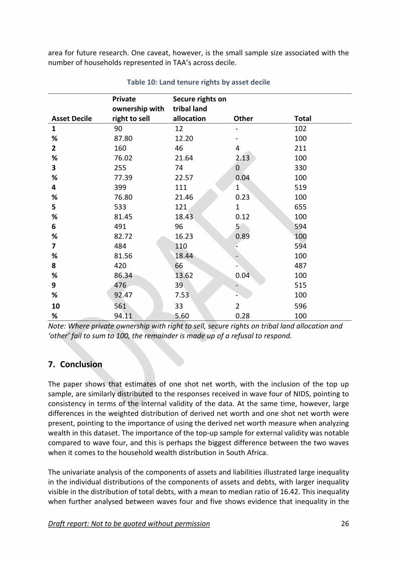
area for future research. One caveat, however, is the small sample size associated with the number of households represented in TAA’s across decile.

Table 10: Land tenure rights by asset decile

Asset Decile

Private ownership with right to sell

Secure rights on tribal land allocation Other Total

1 90 12 - 102 % 87.80 12.20 - 100 2 160 46 4 211 % 76.02 21.64 2.13 100 3 255 74 0 330 % 77.39 22.57 0.04 100 4 399 111 1 519 % 76.80 21.46 0.23 100 5 533 121 1 655 % 81.45 18.43 0.12 100 6 491 96 5 594 % 82.72 16.23 0.89 100 7 484 110 - 594 % 81.56 18.44 - 100 8 420 66 - 487 % 86.34 13.62 0.04 100 9 476 39 - 515 % 92.47 7.53 - 100

10 561 33 2 596 % 94.11 5.60 0.28 100

Note: Where private ownership with right to sell, secure rights on tribal land allocation and ‘other’ fail to sum to 100, the remainder is made up of a refusal to respond.

7. Conclusion

The paper shows that estimates of one shot net worth, with the inclusion of the top up sample, are similarly distributed to the responses received in wave four of NIDS, pointing to consistency in terms of the internal validity of the data. At the same time, however, large differences in the weighted distribution of derived net worth and one shot net worth were present, pointing to the importance of using the derived net worth measure when analyzing wealth in this dataset. The importance of the top-up sample for external validity was notable compared to wave four, and this is perhaps the biggest difference between the two waves when it comes to the household wealth distribution in South Africa. The univariate analysis of the components of assets and liabilities illustrated large inequality in the individual distributions of the components of assets and debts, with larger inequality visible in the distribution of total debts, with a mean to median ratio of 16.42. This inequality when further analysed between waves four and five shows evidence that inequality in the

Draft report: Not to be quoted without permission 27

distribution of assets, debts and net worth has declined, whilst household income inequality has remained the same. At the same time, however, the Gini coefficient on financial assets remains very high. This inequality was reinforced when analyzing the asset shares by asset decile and debt shares by debt decile in South Africa. For both these variables, the median values of assets and debt increase at an increasing rate by decile pointing to large inequality in the components of wealth. In terms of the internal validity of the data, the inclusion of a top up sample of 1005 households bolstered this validity by increasing the mean values of the components of wealth subsequent to weighting and the removal of outliers, bringing the distribution closer to the macroeconomic measures of wealth provided by SARS. However, whilst the internal validity of the data improved through the top up sample, a comparison to SARS’ balance sheet on assets and debt from 2017 still shows some significant differences between NIDS and the national accounts, though nowhere near as large as in wave 4. Financial assets remain under estimated in NIDS wave five. The measure of total debt is also far off the measure provided by SARB. However, the net worth estimates between NIDS and SARB are close, indicating that NIDS does have external validity when looking at wealth through the lens of net worth. Household portfolio composition showed the importance of household possessions as a key constituent of South African asset portfolios, both by asset decile and income decile. The importance of household possessions over the lifecycle was also illustrated with youth owning the highest proportions of household possessions after real estate. At the same time, the analysis of debt composition showed that financial debts are the most prominent types of debts up to the 80th and 70th percentiles of the debt and income distributions in the country bringing into question access to other types of finance by households. The importance of real estate in the asset portfolio composition of the country is also key, this is particularly interesting over geolocation where real estate assets make up over half the asset portfolios of households in urban formal, rural formal and TAA’s. The only exception to this is urban informal areas. At the same time, real estate debt forms only a majority share of debts for households in urban formal areas, highlighting the importance of home ownership: both with a right to sell and with secure tenure from a TAA. Nationally, 14.2 percent of all households are in TAA’s. The distribution of wealth in TAA’s is vastly understudied and this paper opens a window to understanding the relationship between property rights and asset ownership across different land tenure arrangements. We see that there is a varied distribution of asset based wealth across tribal authority areas, with larger proportions of TAA households residing in the middle of the asset distribution. Overall, this paper shows that there is a vast amount of analysis that can be done with the NIDS data on wealth in South Africa. This paper provides a univariate overview of net worth and the components for wealth, but further multivariate and causal analysis across waves are needed.

Draft report: Not to be quoted without permission 28

8. References

Avery, R. B., Elliehausen, G. E., & Kennickell, A. B. (1988). Measuring wealth with survey data: An evaluation of the 1983 survey of consumer finances. Review of income and Wealth, 34(4), 339-369. SARB (South African Reserve Bank), 2018. Balance Sheet: Households and Non-Profit Institutions Serving Households. Historical Macroeconomic Time Series Information. South African Reserve Bank, Pretoria. South African Labour & Development Research Unit (SALDRU) 2018. National Income Dynamics Study, Wave 5 (dataset) Version 1.1. South African Labour & Development Research Unit (producer), Cape Town. DataFirst (distributor).