WFS Iqlo

POLICY RESEARCH WORKING PAPER 1980

The Effect of Household While household wealth isstrongly related to

Wealth on Educational educational attainment of

Attainm ent children nearly everywhere,the magnitude and pattern of

the effect of wealth differs

Demographic and Health Survey widely.Thegapinattainment

Evidence of children of the poor andrich ranges from only one or

two years in some countries

Deon Filmer to nine or ten years in others.

Lant Pritchett This attainment gap is the

result of different patterns of

enrollment and dropout:

while in South America low

attainment among the poor is

almost entirely due to

children who enroll then

drop out early, in West Africa

and South Asia many poor

children never enroll.

The World Bank

Development Research Group

Poverty and Human Resources

September 1998

Pub

lic D

iscl

osur

e A

utho

rized

Pub

lic D

iscl

osur

e A

utho

rized

Pub

lic D

iscl

osur

e A

utho

rized

Pub

lic D

iscl

osur

e A

utho

rized

Pub

lic D

iscl

osur

e A

utho

rized

Pub

lic D

iscl

osur

e A

utho

rized

Pub

lic D

iscl

osur

e A

utho

rized

Pub

lic D

iscl

osur

e A

utho

rized

1II) R \io7 ;ilfi P 'i 1 98(

Summary findings

tI sitig hooseholdo( sur\e e data from 44 Demzograpliic and educational artain merit bet s% r ic ri .i: *

I lCalth Sur\veys in 3,i c ounltrics, Filmer and Pritchett soile countries tile differeiic . rw\r en tilc :'a' pdociiilcit differenit paitternls in the enrollmenlt and in the mnedilan im hiber o, vear ( oo ( ,ni.ete i n

attainment ot children fro(m riclh and poor housellolds. on]x a ear or t\\o; in itlier> t:te giip i i a' great .l - f.-

t lhev find(i that: tenl year .

Fninrollment profiles of the poor differ across * ihc attaililinellt pr tilCs ctll h( :Ied as JIagnlklit

couintries but fall into distinictive regional patterns. In tools to CXamnIeIII iCSueS iII tIIe Cdiicati It I " >t(cI,

soiime areas (including muich of South America) the poor including the cxtent to which enrollime-it ;s low b6eca.ise-

reach nearlv univcrsal enrollnment in first grade but then of the physical uLinavailability ot schools.

drop oUt in droves. In others (including much of South Filmer and Pritchctt ovecrcomile the Lack of data on

Asia and West Africa), the poor never enroll. Both inconme and consumptioni expenditures in the sur\ eys >vh

patterns lead to low attainment. constructing a proxy for longn-run houisehold \xealth.

*'I'here are enormious differences across countries in using survey informationi on asSCt" an11d Using the

the "wealth gap" - the difference in enrollment and statistical techniqUe of principal comnponents.

-T his paper -a product of Poverty and Human Resources, Development Research G.roup - is part of a larger effort in the

groUp to inforimi education policy. The study was funded by the Bank's Research Support Budget under the research project

"Iducational Enrollment and Dropout" (RPO 682-1 1). Copies of this paper are available free from the World Bank, 1818

Hi Street NW, Washingtoni, DC 20433. Please contact Sheila Fallon, roomi MC3-638, telephionie '02-47/3-8009, fax 202-

822-1 153, Internet address sfallonriaworldbank.org. The authors man. he contacted at dfilmer ou orldbank.org or

lpritchett(f worldbank.org. September 1998. (38 pages)

I11e Polioc Rese.rc \Y orking IPaper Series disseminates the findings ot u owk in progrs tS r enicowaiige the exchange ot ideas a.sout

dcle lopnment issues. Ani objectit e of the series is to get the findigs oiut quicklv. ci 'n i th pr 7tesen'ta 1 oins less tkan jUo/K polisoai. [½e

papers .arr the iaoU Sf the authors and should be cited according/v. Tbe fIndings. iwiterpretations ii il .iJ cwlitlsionl s expressedl1 in this

paper are e ntire1% trh(Sc of the authors. Thev do not necessarily represent thec 1ie it ot \t 1,1 Ia UikI !ts Exricutit i Directors, or the

coulntlles tiex rcpreseet.

Produced by the Policy Research D[isseminitiom (Cllntcl

The Effect of Household Wealth on Educational Attainment

Demographic and Health Survey Evidence

Deon Filmer

Lant Pritchett

The Effect of Household Wealth on Educational Attainment Around the World:Demographic and Health Survey Evidence'

Introduction

][n this paper we are interested not just in countries' average educational enrollment and

attainment, for which there has been a great deal of examination both from official and

academJ[c sources, but in how educational attainment differs by household wealth within

countries.2 How much schooling are children from poor households India, Brazil, or Kenya

receiving, both absolutely and relative to the rich in the same country?

Answering this question, especially in a way that produces valid comparisons across

countries is hampered by the limited availability, difficulty of use, and comparability of

household survey data. The Demographic and Health Surveys (DHS), having applied

essentially the same survey instrument in 35 countries potentially overcomes these problems.

One potential limitation of the DHS is that it lacks questions on household income or

consumption expenditures, which are conventionally used as indicators of households'

economic status. However, in a separate methodological paper (Filmer and Pritchett, 1998a)

we shoNv that an index constructed from the questions asked in the DHS about household assets

and housing characteristics (e.g. construction materials, drinking water and toilet facilities)

works as well, and arguably better, than consumption expenditures as a proxy for household

long-run wealth. This finding allows us to use a comparable method, principal components, in

' This work is the result of research developed jointly with Jee-Peng Tan, and it has greatly benefited from herinput. We would also like to thank Emiliana Vegas and seminar participants for helpful comments and suggestions.This research was funded in part through a World Bank Research support grant (RPO 682-1 1).2 Several recent estimates of the stocks of schooling years in many countries have been produced based on theUNESCO Yearbook series enrollment rates and labor free and census surveys (Nehru, Swanson and Dubey, 1993;Barro and Lee, 1993; Dubey and King, 1994; Ahuja and Filmer, 1996).

2

constructing a ranking of households within each country. The "poor" are simply defined as

the bottom 40 percent in each country, so while levels of poverty are not comparable across

countries, the rankings are constructed using a similar method.

An analysis of this data on education and wealth reveals three key findings. First, very

low primary attainment by the poor is driven by two distinct patterns of enrollment and drop-

out. There is a South Asian and Western/Central African pattern in which many of the poor

never enroll in school. In these countries more than 40 percent of poor children never

complete even grade 1 and typically only one in four complete grade 5. In contrast there is a

Latin American pattern in which enrollment in grade 1 is (nearly) universal but drop-out is the

key problem. In South American countries less than 10 percent of the poor never enroll, but

drop-out is so high that median years of school completed is only between 4 and 6 years.

Even though 92 percent of the poor in Brazil complete grade one, only 50 percent of those

complete grade 5. The result is that median attainment of poor children in South America is

less than that of poor children in Ghana, Kenya, or Zimbabwe.

Second, the wealth gaps vary enormously across countries and in most instances raising

the enrollment of the poor will be the key to achieving universal basic education. The

difference in median grade attainment between the poor and rich is very high in South Asia (10

years in India, 9 in Pakistan), high in Latin America and Western/Central Africa (4 to 6 years)

and low in Eastern/Southern Africa (1 to 3 years). Where the wealth gap is large, increasing

the educational attainment of the poor will play the key role in universalizing primary or basic

education. In Colombia and Peru over 70 percent of the shortfall from primary completion is

due to children from the bottom 40 percent of households.

3

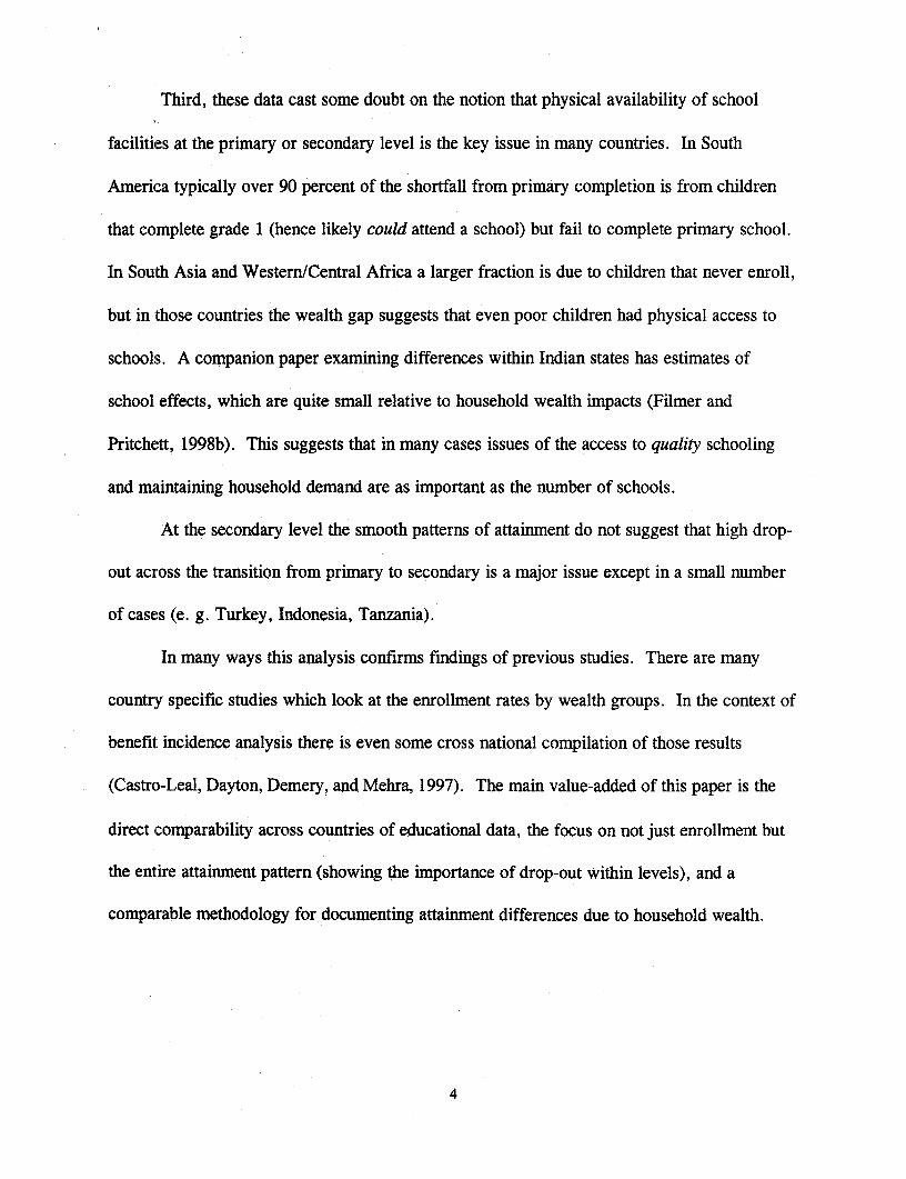
Third, these data cast some doubt on the notion that physical availability of school

facilities at the primary or secondary level is the key issue in many countries. In South

America typically over 90 percent of the shortfall from primary completion is from children

that complete grade 1 (hence likely could attend a school) but fail to complete primary school.

In South Asia and Western/Central Africa a larger fraction is due to children that never enroll,

but in those countries the wealth gap suggests that even poor children had physical access to

schools. A companion paper examining differences within Indian states has estimates of

school effects, which are quite small relative to household wealth impacts (Filmer and

Pritchett, 1998b). This suggests that in many cases issues of the access to quality schooling

and maintaining household demand are as important as the number of schools.

At the secondary level the smooth patterns of attainment do not suggest that high drop-

out across the transition from primary to secondary is a major issue except in a small number

of cases (e. g. Turkey, Indonesia, Tanzania).

In many ways this analysis confirms findings of previous studies. There are many

country specific studies which look at the enrollment rates by wealth groups. In the context of

benefit incidence analysis there is even some cross national compilation of those results

(Castro-Leal, Dayton, Demery, and Mehra, 1997). The main value-added of this paper is the

direct comparability across countries of educational data, the focus on not just enrollment but

the entire attainment pattern (showing the importance of drop-out within levels), and a

comparable methodology for documenting attainment differences due to household wealth.

4

I) Data and Methods

A) The Demographic and Health Surveys

The Demographic and Health Surveys (DHS) are large nationally representative

household surveys.3 The surveys have been carried out using a nearly identical survey

instrument in over fifty developing countries.4 While the main purpose of the surveys is to

inquire about family planning and child and maternal health, the surveys also contain an

educational history of all household members from a chosen respondent.

The education variables we analyze are based on four questions:

* Has [name] ever been to school?

* If attended school:

what is the highest level of school [name] attended?

what is the highest grade/years [name] completed at that level?

* If attended school:

Is [name] still in school?

These questions are used to construct an " attainment" history for a recent cohort, those aged

15 to 19 inclusive. This attainment profile is the proportion of the cohort who have completed

any given grade or higher.

The analysis so far has covered 35 countries. Countries have been grouped into six

regions. The groups, ranked from lowest to highest median attainment of the bottom 40

'Table 1 shows that the samples of individuals in the 15-19 age range are usually above 2,000, but vary from1,355 in Kazakhstan to over 50,000 in India.4 There are three main designs of the survey instrument. DHS I surveys were carried out between 1985 and 1989,DHS II between 1990 and 1993, and DHS III are those that have been carried out since 1994.

5

percent are: Westem/Central Africa, South Asia, Central America and Caribbean, South

America, Eastern/Southern Africa, East Asia, and Central Asia / North Africa / Europe.

B) Constructing an "asset index"

The DHS do not ask about household income or consumption expenditures, but the

DHS [E and III survey instruments do include two sets of questions related to the economic

status of the household. First, households are asked about their ownership of various assets,

such as whether any member owns a radio, a television, a refrigerator, a bicycle, a

motorcycle, or a car. Second, they are asked about characteristics of their housing, namely

whether electricity is used, the source of drinking water, the type of toilet facilities, how many

rooms there are for sleeping, and the type of materials are used in the construction of the

dwelling. There is substantial overlap in the questions asked in each country, but the precise

list varies. The number of variables constructed from these questions is usually 15 or 16 but

varies from 12 to 21 (last column of Table 1).

In order to use these variables to rank households by their economic status, they need to

be aggregated into an index and of course the main problem in constructing such an index is

choosing appropriate weights.5 We use the statistical technique of principal components to

derive weights. Principal components is a technique for summarizing the information contained

in a set of variables to a smaller number by creating a set of mutually orthogonal components of

the data. Intuitively, the first principal component is that linear index of the underlying variables

that captures the most common variation among them.

If these assets were only to be used to used examine the impact of some other factor (e.g., maternal education)as a "control" for wealth in a multivariate regression we would not need to aggregate the variables (Montgomery,Burke, Paredes, and Zaidi, 1997)

6

Table 1: Summary informationCountry Year Number of Proportion of Value of Ist Difference Number of

households variance eigen value between Ist and assetsexplained by Ist 2nd eigen

PC valuesWestem and Central AfricaBenin 1993 4499 0.268 4.293 2.722 16Burkina Faso 1992-93 5143 0.276 4.005 2.270 1 5Cameroon 1991 3358 0.247 3.809 2.032 15C.A.R. 1994-95 5551 0.240 3.845 1.961 16Cote d'lvoire 1994 5935 0.223 3.341 1.670 15Ghana 1993 5822 0.211 3.166 1.618 15Mali 1995-96 8716 0.230 3.448 1.430 15Niger 1992 5242 0.265 4.234 2.553 16Nigeria 1990 8999 . . . 0Senegal 1992-93 3528 0.231 3.554 2.043 15South AsiaBangladesh 1993-94 9174 0.285 3.987 2.334 14Bangladesh 1996-97 8682 0.309 4.018 2.460 13India 1992-93 87175 0.256 5.368 3.713 21Nepal 1996 8082 0.219 2.622 0.898 12Pakistan 1990-91 7193 0.283 4.237 2.704 15Central AmericaDominican Republic 1991 7144 0.249 4.227 2.676 17Dominican Republic 1996 8831 0.241 3.848 2.372 16Guatemala 1995 11297 0.264 3.958 2.534 15Haiti 1994-95 4818 0.266 3.987 2.230 15South AmericaBolivia 1993-94 9114 0.311 3.732 2.347 12Northeast Brazil 1991 6064 0.263 4.204 2.860 16Brazil 1996 13283 0.226 3.163 1.261 14Colombia 1990 7412 0.216 3.246 1.970 15Colombia 1995 10112 0.240 3.606 2.325 15Paraguay 1990 6348 . . . 0Peru 1991-92 13479 0.283 4.238 2.878 15Peru 1996 28122 0.267 4.001 2.540 15Eastern and Southern AfricaComoros 1996 2252 0.230 3.453 1.738 15Kenya 1993 7950 0.264 3.961 2.362 15Malawi 1992 5323 0.186 2.598 1.071 14Namibia 1992 4101 0.300 4.499 3.051 15Rwanda 1992 6252 0.200 2.798 1.308 14Tanzania 1991-92 8327 0.187 2.798 1.001 15Tanzania 1996 7969 0.202 3.036 1.114 15Uganda 1995 7550 0.192 2.886 1.023 15Zambia 1992 6209 0.259 3.879 2.108 15Zambia 1996-97 7286 0.275 4.121 2.695 15Zimbabwe 1994 5984 0.273 4.101 2.216 15East Asia and PacificIndonesia 1991 26858 0.296 2.665 1.051 9Indonesia 1994 33738 0.258 3.352 1.585 13Philippines 1993 12995 0.257 3.596 2.200 14Middle East, North Africa, and EuropeEgypt 1992 10760 0.266 3.452 1.943 13Egypt 1995-96 15567 0.250 3.255 1.861 13Kazakhstan 1995 4178 0.203 3.045 1.479 15Morocco 1992 6577 0.286 4.571 3.163 16Turkey 1993 8612 0.234 2.806 1.511 12

Unweighted average 10687 0.250 3.659 2.065 14Unweighted std dev 13093 0.032 0.605 0.659 3.5Median 7481 0.256 3.771 2.154 15

7

'We assume that the most "common variation" in the set of asset variables is a good

proxy for a household's wealth. Filmer and Pritchett (1998a) defends this assumption,

showing the asset index performs as well as a more traditional measures, such as household

size adjusted consumption expenditures. Empirical estimates in that paper suggest that the

asset index works as well, or better, as a proxy for long-run household wealth to predict

childreii's enrollment than consumption expenditures. There are two key findings that suggest

assets might work "better". First, the enrollment profile is consistently "flatter," that is it

shows smaller gaps between rich and poor, when using expenditures as opposed to assets,

which is consistent with a large transitory component in expenditures. Second, in three

countries with surveys where the results of asset index and consumption expenditures could be

compared for the same households, the comparison of OLS and instrumental variables

estimates and of bounds from reverse regression suggest that consumption expenditures has

considerably more measurement error as a proxy for predicting enrollments than does the asset

index. We wish to stress that we do not imply that the asset index is a proxy for current

standards of living, nor that it is appropriate for poverty analysis.

The fourth column of Table 1 shows how well the first principal component of the asset

variables (which is our asset index) "fits" the underlying variables, reporting the proportion of

the variation captured. The proportion is remarkably stable, and reasonably high, at between

20 and 30 percent of the variance (from Uganda at .19 to Bolivia at .31)6.

There is a generic problem with principal components analysis. While it is relatively

easy to interpret the first principal component, an intuitive explanation of the second and

8

higher order components is more problematic. Analysts generally hope for only one factor.

In our case, although the first eigen value is relatively high, it is not as high as we would have

liked and the value of the second eigen value is also generally above 1, the commonly used

cut-off value for "significant" components. This suggests that the "co-movement" of the

assets is explained by more than one factor. We have no idea how to interpret this second

principal component (especially in a consistent way across countries) and will ignore it for

now in an uneasy truce with the data. We do believe, however, that it is not an unreasonable

assumption that the "factor" which explains the largest amount of the " co-movement" of the

different assets can be interpreted as a household's economic status7.

The asset index is calculated separately for each country. Within each country

individuals are sorted by the asset index and cutoffs for the bottom 40 percent, the middle 40

percent, and the top 20 percent are derived. Households are then assigned to each of these

groups on the basis of their value of the asset index. From here on we will refer to these

groups, without further apology, as "poor", "middle" and "rich" .'

Since the principal components procedure normnalizes the mean of the index to zero

for each country, the value of the index is zero for all countries. Therefore, in comparing the

"poor" in Kenya to the "poor" in Turkey or India it is important to keep in mind that the

measure is relative and 40 percent of the households are defined to be "poor" in every

6 Since random measurement error will tend to "flatten" the household wealth / enrollment relationship the factthat the fit is similar across countries is comforting as the cross-country comparisons are therefore not likely to begreatly affected by differing degrees of measurement error.7 Since, by construction, principal components are orthogonal to one another, the "omitted variables" problem ofignoring the second principal component should not be severe. But this rationalization would not be true of omittedvariable bias for additional control variables, such as urban residence, which may be correlated with eithercomponent.8 While the cut-off is based on all individuals, the analysis is carried out only for those 15 to 19 so there can bemore or less than 40 percent of that cohort in the bottom 40 percent of households.

9

country. Moreover, the gap between rich and poor could easily vary between countries so the

Brazilian poor could well be relatively poorer than the Brazilian rich compared to the Egyptian

poor relative to the Egyptian rich.

C) Attainment Profiles

'We use the data for children aged 15 to 19 to create an "attainment profile" which

shows graphically the proportion of individuals that completed each grade or higher (Figure

1). For example this means that the level at grade 1 shows the proportion that ever attended

school and completed first grade. One minus this proportion is the proportion that never

completed even one year of schooling.9 The slope of the enrollment profile is a simulation of

drop-outs.'0 The difference between the proportion that completed grade 5 or higher and those

that completed grade 6 or higher is an estimate of the proportion of all children that dropped

out between 5th and 6th grade. This is not the usual drop-out rate, as the denominator is all

children as opposed to the proportion of those reaching 5th. In the attainment profile figures

the drop-out rate is the vertical drop between grades as a proportion of the absolute height.

Figure 1 shows the attainment profiles for each of the 35 countries (some with profiles

for more than one survey) with the profile of the poor, middle and rich identified. Since much

of the paper is an exploration of the interesting results and patterns that emerge from these

graphs we'll walk through the interpretation of the graphs by describing the first country,

Benin in detail.

9 We are therefore not distinguishing between attending school but never completing even one grade and neverhaving attended school at all.0 This is a simulation because we are not observing an individual's progression through the school system but a

cross section of attaimnents of this cohort.

10

Figure 1Attainment profiles for ages 15 to 19, by economic group:

Western and Central Africa

Benin 1993 Burkina Faso 1991-92 I Cameroon 1991

1l 1l- °11 ,

0.8 i 0.8 i 0.81

'0.6 00.6 a \0.6

'0.4 0.4 0.4

0.2 0.2- 0.2 _

0 00

1 2 3 4 5 6 7 8 123456789 1 2 3 4 5 6 7 8 9Grade I Grade Grade

C.A.R. 1994-95 Cote d'lvoire 1994 Ghana 1993

0.8 0.8 0.

_ 0.6 0- e , EO.6 0.6 -

0.4 ~~~~~~~04 04-

0.2 >>*>0.2 0.20 ~~~ ~ ~~~~0 +9 0

1 2 3 4 5 6 7 8 9 1 2 3 4 5 6 7 89 1 2 3 4 5 6 7 89Grade Grade Grade

Mali 1995-96 Niger 1992 Senegal 1992-93. ~~~~I ] _ _ _ _ ,

0.8 . 0.8 1 0.8 -

.~0.6 - - 0.6 o0.6 -

o04 E 0.4 04

0.2 - 0.2 0.2

0 0~ 01

1 2 3 4 5 6 7 8 9 1 2 3 4 5 6 7 89 1 2 3 4 5 6 7 89Grade I Grade Grade

* Poorest . Middle A Richest

11

Figure 1 continued

Attainment profiles for ages 15 to 19, by economic group:

South Asia

Bangladesh 1993-94 Bangladesh 1996-97 India 1992-93

1.l i 1 ol

0.8 0.8-- 0.8

'o0.6 - I 0.6 -- < e 0.6l0.6 0.6 0.6

20.4 0.4 0.4

0.2 0.2 0.2

0 0 0

1 2 3 4 5 6 7 8 9 1 2 3 4 5 6 7 8 9 1 2 3 4 5 6 7 8 9Grade Grade Grade

Nepal 1996 Pakistan 1990-91

0.8 -- 0.8

20.6 ~0.6 . -

0.4 0.4

0.2 0.2- -

0 0 I

1 2 3 4 5 6 7 8 9 1 2 3 4 5 6 7 8 9Grade Grade

* Poorest u Middle A Richest

12

Figure 1 continuedAttainment profiles for ages 15 to 19, by economic group:

Central America and Caribbean

pominican Republic 1991 prnminican Republic 1996 Guatemala 1995

08 0 8 08

06 ~~~~~~~~ 06 06

0 4 0 4 04

04 2 04 2 04

02 02 02

1 2 3 4 5 6 7 8 9 1 2 3 4 5 6 7 8 9 1 2 3 4 5 6 7 8 9Grade Grade Grade

Haiti 1994-95

0.8

0 2

i 2 3 4 5 6 7 8 9Grade

* Poorest * Middle A Richest

13

Figure 1 continued

Attainment profiles for ages 15 to 19, by economic group:

South America

Bolivia 1993-94 Northeast Brazil 1991 Brazil 1996

0 8.81 8 --- 0.8

08|D O 10 6 00.6-o0.6-006 ----- 0-

0. 04-04

U.2 . . ) 1 0.2 0.200

0 . o - ! - o - 0 2 , 0 . 2

1 2 3 4 5 6 7 8 9 1 2 3 4 567891 2 3 4 5 6 7 8 9Grade Grade Grade

Colombia 1990 Colombia 1995 i Peru 1991-92

0.8-- 0.8 - --

s 0.6 1< = 0.6 | 408o.6

[ N 0.4 -\<, \; ; I :; 0.4 E . 0.4 0.

0.2 -0.2 -0.2 - - -

0 - 0 _ __ _0 ____

1 2 3 4 5 6 7 8 9 1 2 3 4 5 6 7 89 1 2 3 4 5 6 7 8 9Grade Grade Grade

Peru 1996 [Northeast Brazil 19961

0.8 0.8 - -

0.6 e 0.6

0.4 0.4

0.2- -- 0.2 .-

O-- 0- : 1 2 3 4 5 6 7 8 9 1 2 3 4 5 6 7 8 9

Grade Grade

* Poorest . Middle A Richest

14

Figure 1 continuedAttainment profiles for ages 15 to 19, by economic group:

Eastern and Southern Africa

Comoros 1996 Kenya 1993 Malawi 1992

- - -. ---------- -. - -.--- ..... --.- ------------- .-----------

0~8 0.8 -0.8-

s 0~6 ;0 eg 06- 0g.6

024 02 4 02

0 20- 2 0 2

1 2 3 4 5 6 7 8 9 1 2 3 4 5 6 7 8 9 1 2 3 4 5 6 7 8 9Grade Grade Grade

f~~~~~~~~~~~t.~~~~~~~ I

Namlbia 1992 Rwanda 1992 Tanzania 1991-92ll I~ ~ ' ............................................................---- .r....=

0.8- 08- 0.8 -

O S606 \0 6

IC 4 0 404

a. 04 -- - - 0.04- --- - :04 \

02 - 0.2 0.2

O 0 0-

1 2 3 4 5 6 7 8 9 I 2 3 4 5 6 7 8 9 1 2 3 4 5 6 7 8 9Grade Grade Grade

Tanzania 1996 Uganda 1995 Zambia 1992

0 8 0.84 1 0.81-

06 0.606

a. 4 0.4a. 04

02 -- - 02 0.2-

0 0 o__ _ _ _ _ _

I 2 3 4 5 6 7 8 9 I 2 3 4 5 6 7 8 9 1 2 3 4 5 6 7 8 9Grade Grade Grade

* Poorest u Middle A Richest

15

Figure 1 continuedAttainment profiles for ages 15 to 19, by economic group:

Eastern and Southern Africa continued

Zambia 1996-97 Zimbabwe 1994

084 < > 0.8 N i

O 0,6

t 04 a 404

02 - 02

0 0

1 2 3 4 5 6 7 8 9 1 2 3 4 5 6 7 8 9Grade Grade

Attainment profiles for ages 15 to 19, by economic group:East Asia and Pacific

Indonesia 1991 I Indonesia 1994 Philippines 1993

08- 0.8 08.

0.6 0.6 0.6

a., 04 c_ 0.4 a.0.4

02 0.2 _ 0.2

0 0 I~~~~~ 01 2 3 4 5 6 7 8 9 1 2 3 4 5 67 89 I 1 2 3 4 5 6 7 8 9

Grade Grade Grade

* Poorest * Middle & Richest

16

Figure 1 continued

Attainment profiles for ages 15 to 19, by economic group:

Middle East, North Africa, Central Asia and Europe

Egypti 1992 Egypt 1995-96 Kazakstan 1995

08 ~~~ - -> } 086____+ _0 08

0 6 0 0.6 0 6

0.2 02. 0.2

o O O

0 4 a. 4 0. 04

~2 02 0.2

0 . 0

1 2 3 4 5 6 7 8 9 1 2 3 4 5 6 7 8 9 1 2 3 4 5 6 7 8 9Grade Grade Grade

Morocco 1992 Turkey 1993

08 4 08

02 02 0

3 0

1 2 3 4 5 6 7 8 9 1 2 3 4 5 6 7 8 9Grade Grade

* Poorest . Middle A Richest

17

Figure 2 In Benin (whose attainment profile is reproduced in

Benin 1993 Figure 2) only 26 percent of the poor aged 15 to 19 have

completed of grade 1 or higher, so 74 percent have either0.8

.o 0.6 >- . | attended school (or more precisely, not completed even one

>,, 0.4 - ~ > < ( year of schooling). Completion of grade 5 or higher is only

0.2 J 7.9 percent and only 0.7 percent complete grade 9. Among

0 the rich, 80 percent complete grade 1 or higher but drop-out1 2 3 4 5 6 7 8 9

Gradeis such that only 54 percent complete grade 5. Even among

* Poorest * Middle A Richestthe rich only 17 percent complete grade 9.

We define two "wealth gaps". First, the wealth gap in the completion of any given

grade (which, graphically, is the vertical distance between economic groups). For example,

the wealth gap in grade 1 completion is .54 in Benin (.74 for the rich versus .20 for the poor

with no schooling), while the wealth gap at grade 5 is .46. Second, the wealth gap in median

grade completed. Visually the median is where a horizontal line at .5 would cross the

attainment profile hence the gap is, graphically, the horizontal distance between the two

groups. The median grade completed of the poor in Benin is zero, while that of the middle

group is 2, and that of the rich is 5 years. The wealth gap in attainment is 5 years.

There are three main patterns that emerge from these figures and they are discussed in

turn.

* First, the role of "ever enrollment" versus drop-out in explaining education

outcomes,

* second, differing wealth gaps and attainment patterns across countries,

18

* and third, the use of the differences in attainment profiles as a diagnostic tool.

II) Enrollment and drop-out among the poor

Average attainment can be decomposed into two parts: the fraction of children that ever

enroll and, conditional on having enrolled, the grade at which children leave school. We do

not distinguish between those who never enrolled and those who may have enrolled but did not

complete even one year of schooling, and in the following discussion the two descriptions are

used interchangeably.

A) Patterns of enrollment and dropout

There are four patterns of enrollment and drop-out of the poor, which tend to follow

regional patterns:

* low ever enrollment and high drop-out (Western/Central Africa)

* low ever enrollment and low drop-out (South Asia)

* high ever enrollment and early high drop-out (Latin America)

* high ever enrollment and late (East Africa) or very late drop-out (East Asia and

Central Asia/North Africa/Europe).

Table 2 presents the proportion of 15 to 19 year olds from the poorest 40 percent who

completed (at least) grade 1, grade 5, primary school, and grade 9. Because the lengths of the

cycles (primary versus lower secondary --sometimes together called "basic"-- and upper

secondary) differ across countries we show the results both for the comparable number of

grades (grade 5) and for the comparable cycle (primary)." Grade 9 was chosen as the highest

"Presently we are using the UNESCO reporting of the structure of primary and secondary, which may or may notreflect country realities and moreover, may not have been relevant to the situation a decade ago.

19

grade to report because the truncation problem (that children are still in school and we are not

observing completed spells of schooling) becomes more severe the higher the grade.

In Western/Central Africa only between 4.6 (Mali) and 27 (Cote d'Ivoire) percent of

poor children complete grade 5. This is a combination of low ever enrollment and substantial

drop-out. For instance, in Benin 74 percent never completed even grade 1 and of those that

did, oinly 30 percent complete grade five leaving overall completion of grade 5 at only 8

percerLt.

In South Asia the fraction of poor children who didn't complete grade 1 is also very

high, around 50 percent, but of those children that do start there is much higher retention.

Having begun school between 55 (Bangladesh) and 80 (India) percent stay through to grade 5,

but after that drop-out accelerates.

The Latin American pattern is one of high initial enrollment, but very steep drop-out

among the poor. The situations are strikingly similar especially within South America where

almost all poor children start school: the percent never enrolled ranges from 4.2 (Bolivia) to

7.6 (Brazil), but subsequent drop out is high. In all four South American countries the

attaimnent profile of the poor drops sharply while the middle and rich children stay in school.

In Brazil only 49 percent of those that complete grade 1 go on to complete grade 5. The

situation is even bleaker when looking at the entire 6 to 8 years of primary school. Of those

that complete grade 1 only 16 percent in Brazil go on to complete primary school, in Bolivia

only 30 percent do so.

20

Table 2: Completion and simulated transition proportions for the poorest 40 percentDidn't Completed Completed Completed

Country Year Years in Grade I Grade 5 Primary Grade 9 complete grade 5 primary grade 9primary even grade of those of those of thosecycle I who who who

completed completed completed1 1 5

Western and Central AfricaBenin 1993 6 0.264 0.079 0.036 0.007 0.736 0.300 0.136 0.091Burkina Faso 1992-93 6 0.130 0.078 0.064 0.002 0.870 0.599 0.488 0.030C.A.R. 1991 6 0.514 0.148 0.047 0.003 0.486 0.288 0.091 0.022Cote d'lvoire 1994-95 6 0.419 0.271 0.158 0.039 0.581 0.646 0.376 0.144Cameroon 1994 6 0.640 0.446 0.318 0.055 0.360 0.697 0.497 0.124Ghana 1993 6 0.791 0.694 0.652 0.306 0.209 0.877 0.825 0.441Mali 1995-96 6 0.119 0.046 0.025 0.001 0.881 0.386 0.208 0.032Niger 1992 6 0.154 0.113 0.016 0.007 0.846 0.739 0.102 0.062Rwanda 1992 8 0.730 0.469 0.147 0.037 0.270 0.643 0.201 0.080Senegal 1992-93 6 0.199 0.143 0.108 0.017 0.801 0.716 0.542 0.118South AsiaBangladesh 1993-94 5 0.497 0.274 0.274 0.063 0.503 0.551 0.551 0.230Bangladesh 1996-97 5 0.588 0.356 0.356 0.080 0.412 0.606 0.606 0.223India 1992-93 5 0.472 0.376 0.376 0.139 0.528 0.797 0.797 0.369Nepal 1996 5 0.594 0.406 0.406 0.116 0.406 0.683 0.683 0.287Pakistan 1990-91 5 0.328 0.250 0.250 0.065 0.672 0.761 0.761 0.260Central AmericaDominican Republic 1991 6 0.912 0.560 0.427 0.111 0.088 0.614 0.469 0.198Dominican Republic 1996 6 0.873 0.569 0.466 0.143 0.127 0.652 0.534 0.251Guatemala 1995 6 0.680 0.236 0.182 0.022 0.320 0.347 0.268 0.091Haiti 1994-95 6 0.724 0.161 0.099 0.018 0.276 0.223 0.137 0.110South AmericaBolivia 1993-94 8 0.958 0.705 0.288 0.195 0.042 0.737 0.301 0.276Northeast Brazil 1991 8 0.754 0.121 0.009 0.009 0.246 0.160 0.012 0.074Brazil 1996 8 0.924 0.457 0.150 0.078 0.076 0.494 0.162 0.172[Northeast Brazil] 1990 8 0.879 0.344 0.093 0.046 0.121 0.392 0.106 0.133Colombia 1990 5 0.941 0.571 0.571 0.096 0.059 0.607 0.607 0.168Colombia 1995 5 0.939 0.630 0.630 0.145 0.061 0.671 0.671 0.230Peru 1991-92 6 0.974 0.813 0.624 0.217 0.026 0.834 0.641 0.267Peru 1996 6 0.954 0.746 0.496 0.175 0.046 0.781 0.520 0.235Eastern and Southern AfricaComoros 1996 6 0.576 0.280 0.173 0.014 0.424 0.485 0.300 0.048Kenya 1993 7 0.963 0.835 0.520 0.102 0.037 0.866 0.540 0.122Malawi 1992 8 0.666 0.291 0.066 0.011 0.334 0.437 0.099 0.038Namibia 1992 7 0.918 0.528 0.223 0.047 0.082 0.575 0.243 0.090Tanzania 1991-92 7 0.821 0.676 0.486 0.004 0.179 0.824 0.592 0.006Tanzania 1996 7 0.803 0.618 0.376 0.004 0.197 0.770 0.468 0.007Uganda 1995 7 0.784 0.390 0.130 0.027 0.216 0.498 0.165 0.069Zambia 1992 7 0.819 0.524 0.255 0.008 0.181 0.640 0.311 0.015Zambia 1992 7 0.858 0.537 0.254 0.033 0.142 0.626 0.296 0.061Zimbabwe 1994 7 0.973 0.892 0.696 0.252 0.027 0.917 0.716 0.283East Asia and PacificIndonesia 1991 6 0.946 0.778 0.713 0.186 0.054 0.822 0.753 0.240Indonesia 1994 6 0.959 0.787 0.730 0.190 0.041 0.821 0.761 0.242Philippines 1993 6 0.973 0.801 0.735 0.320 0.027 0.824 0.755 0.400Middle East, North Africa, and EuropeEgypt 1992 6 0.718 0.639 0.571 0.374 0.282 0.889 0.796 0.586Egypt 1995-96 6 0.745 0.631 0.572 0.396 0.255 0.846 0.767 0.628Kazakhstan 1995 4 0.995 0.994 0.995 0.833 0.005 0.999 1.000 0.838Morocco 1992 6 0.366 0.211 0.106 0.029 0.634 0.576 0.289 0.136Turkey 1993 5 0.932 0.910 0.910 0.186 0.068 0.976 0.976 0.204

21

One of the most striking findings to emerge from these results is that the level of

attainment of the poor in Latin America is lower, not only than East Asia, but even than

Eastern/Southern Africa. Grade 5 completion among the poor is 46 percent in Brazil, 57

percent in the Dominican Republic, 63 percent in Colombia, and peaks at 75 percent in Peru.

In contrast, it is 89 percent in Zimbabwe, 84 percent in Kenya, 69 percent in Ghana, and 62

percent in Tanzania. The only Eastern/Southern African country with lower attainment for its

poor than Brazil is Uganda.

The Eastern/Southern African countries have, by and large, relatively low drop out

rates in the primary years. So, while the fraction who never enroll is similar to that in the

South American countries, the better Eastern/Southern African countries retain higher

proportions of the poor. This is especially clear in the flat portions in Figure 1 of the profile

for the poor in Kenya, Tanzania, and Zimbabwe (and Ghana, which although it is in West

Africa has the attainment patterns of Eastern/Southern Africa).

The final pattern is relatively high attainment countries with both high enrollment and

high retention through primary and beyond into lower secondary. The patterns differ between

Indonesia and Turkey with sharp drop-offs in attainment between primary and secondary and

the Philippines and Egypt with less sharp changes across primary to secondary, a difference

we return to below.

B) Reaching universal attainment and the poor

Nearly every country in the world has set a goal to reach universal educational

attainmnent through some level: primary, "basic," or even secondary. One important question

is what remains to be accomplished to achieve this goal. Examining the attainment profiles in

Figure 1 it is clear that in some countries it is practically only the poor who are not completing

22

primary school while in other countries it is both the middle and poorest groups who do not do

so. In only a very few countries do the rich not already have universal basic attainment.

In Table 3 we report the deficit from universal completion of grade 5 and of primary

school. In Figure 1 the shortfall is the vertical distance shown from the horizontal line at

universal completion (value of 1) to the level who have completed the grade in question. We

then decompose this deficit into that fraction due to shortfalls of the poor, the middle, and the

rich children. 2

Again, there are regional patterns in the absolute level of the shortfall and in the

fraction of that shortfall due to the different groups. Western/Central Africa has high levels of

deficit from grade 5 attainment (around 80 percent) which are nearly evenly distributed across

wealth groups. This counter-intuitive result stems partially from the fact that the asset index is

defined on a household, not per capita basis. In these cases there are substantially more than

20 percent of children in the top 20 percent of households (the percentage ranges from 23

percent in Comoros to 27 percent in Cote d'Ivoire).

In South Asia the attainment deficit is large but its distribution varies. In India and

Pakistan the large wealth gaps are revealed in a concentration of the attainment deficit in the

poor and middle groups. For India there is a 38 percent shortfall from completion of grade 5,

of which 61 percent is due to children from the bottom 40 percent of households while only 4

percent is due to children from the richest 20 percent.

12 That is, for example, the fraction due to the poor is Sp*pp/S where Sp is the shortfall for the poorest group, pp isthe proportion of 15 to 19 year olds that are in the poorest group, and S is the total shortfall.

23

Table 3: Shortfall from grade 5 and primary completion, and the proportion of that shortfall due to theshortfall in each economic group

Shortfall from grade 5 completion Shortfall from primary completionTotal Proportion Proportion Proportion Total Proportion Proportion Proportion

Country Year due to due to due to due to due to due topoorest 40 middle 40 richest 20 poorest 40 middle 40 richest 20percent percent percent percent percent percent

Western and Central AfricaBenin 1993 0.706 0.443 0.385 0.172 0.797 0.411 0.395 0.193Burkina Faso 1992-93 0.749 0.443 0.414 0.143 0.775 0.435 0.413 0.152C.A.R. 1991 0.643 0.478 0.388 0.134 0.796 0.432 0.393 0.175Cote d'Ivoire 1994-95 0.552 0.434 0.395 0.171 0.674 0.410 0.403 0.187Cameroon 1994 0.350 0.569 0.365 0.065 0.481 0.509 0.389 0.101Ghana 1993 0.251 0.440 0.456 0.103 0.292 0.429 0.457 0.112Mali 1995-96 0.804 0.411 0.422 0.167 0.848 0.398 0.418 0.184Niger 1992 0.800 0.394 0.456 0.150 0.914 0.383 0.444 0.173Rwanda 1992 0.455 0.417 0.403 0.180 0.780 0.391 0.421 0.188Senegal 1992-93 0.640 0.498 0.390 0.112 0.694 0.478 0.398 0.124South AsiaBangladesh 1993-94 0.524 0.463 0.447 0.090 0.524 0.463 0.447 0.090Bangladesh 1996-97 0.465 0.500 0.394 0.106 0.465 0.500 0.394 0.106India 1992-93 0.378 0.606 0.357 0.037 0.378 0.606 0.357 0.037Nepal 1996 0.512 0.442 0.441 0.117 0.512 0.442 0.441 0.117Pakistan 1990-91 0.500 0.531 0.403 0.066 0.500 0.531 0.403 0.066Central America and CaribbeanDominican Republic 1991 0.264 0.636 0.266 0.099 0.360 0.607 0.301 0.092Dominican Republic 1996 0.254 0.668 0.262 0.070 0.329 0.638 0.286 0.076Guatemala 1995 0.450 0.589 0.345 0.066 0.508 0.559 0.368 0.073Haiti 1994-95 0.557 0.494 0.361 0.145 0.663 0.446 0.396 0.158Bolivia 1993-94 0.145 0.684 0.211 0.106 0.395 0.608 0.301 0.091South AmericaNortheast Brazil 1991 0.649 0.495 0.337 0.169 0.917 0.395 0.393 0.214Brazil 1996 0.322 0.698 0.236 0.066 0.649 0.542 0.325 0.133[Northeast Brazil] 1996 0.517 0.810 0.162 0.028 0.808 0.716 0.238 0.045Colombia 1990 0.232 0.674 0.234 0.092 0.232 0.674 0.234 0.092Colombia- 1995 0.191 0.737 0.196 0.068 0.191 0.737 0.196 0.068Peru 1991-92 0.091 0.741 0.169 0.090 0.189 0.710 0.202 0.088Peru 1996 0.118 0.756 0.173 0.071 0.244 0.723 0.207 0.071Eastern arnd Southern AfricaComoros 1996 0.543 0.463 0.406 0.130 0.686 0.421 0.429 0.149Kenya 1993 0.171 0.388 0.470 0.143 0.467 0.412 0.464 0.124Malawi 1992 0.584 0.461 0.409 0.130 0.865 0.411 0.408 0.182Namibia 1992 0.350 0.549 0.408 0.043 0.633 0.500 0.425 0.075Tanzania 1991-92 0.255 0.477 0.409 0.116 0.430 0.449 0.414 0.138Tanzania 1996 0.306 0.445 0.442 0.113 0.535 0.415 0.448 0.136Uganda 1995 0.478 0.531 0.368 0.101 0.756 0.479 0.391 0.130Zambia 1992 0.256 0.667 0.290 0.042 0.508 0.526 0.366 0.107Zambia 1992 0.295 0.565 0.400 0.036 0.546 0.492 0.415 0.094Zimbabwe 1994 0.078 0.551 0.358 0.092 0.216 0.563 0.384 0.053East Asiza and PacificIndonesia 1991 0.125 0.622 0.317 0.061 0.166 0.605 0.328 0.067Indonesia 1994 0.118 0.627 0.289 0.084 0.153 0.615 0.309 0.076Philippines 1993 0.093 0.738 0.205 0.057 0.127 0.716 0.217 0.066Middle East, North Africa, and EuropeEgypt 1992 0.214 0.688 0.248 0.064 0.272 0.642 0.284 0.074Egypt 1995-96 0.220 0.673 0.258 0.069 0.265 0.646 0.277 0.077Kazakhstan 1995 0.007 0.396 0.568 0.037 0.007 0.356 0.605 0.039Morocce 1992 0.495 0.599 0.327 0.073 0.627 0.536 0.372 0.091Turkey 1993 0.068 0.551 0.368 0.080 0.068 0.551 0.368 0.080

24

Consistent with the previous observations, the large drop-out rates of the poor in Latin

America are revealed in the large proportions of the deficit that is due to the poor. In South

America the fraction that do not complete grade 5 is between 12 (Peru) and 32 (Brazil) percent

but over 70 percent of that shortfall is due to the poor. The attainment deficit problem for

these countries is essentially keeping the poor in school.

The Eastern/Southern African countries are again a contrast with those in both

Western/Central Africa and Latin America. The shortfalls from grade 5 completion are much

lower than those in Western/Central Africa or South Asia and somewhat higher than those in

South America, but the distribution of the shortfall is more even. This is true especially when

looking at the entire primary school cycle, where the fraction due to the poorest and middle

groups is roughly equal.

Finally, in East Asia the gaps are smaller, but concentrated among the poor. In the

Philippines there is only a 13 percent shortfall from universal primary completion, of which 72

percent is due to the shortfall of the poor.

III) "Wealth gaps" across countries

The second prominent feature of the country profiles in Figure 1 is the uniform ranking

of the rich, middle and poorest groups in terms of educational attainment. As discussed above

there are two ways to define a wealth gap. First, the difference in the proportion of each

group who complete any given grade. Second, the difference in the median attainment of rich

and poor groups.

25

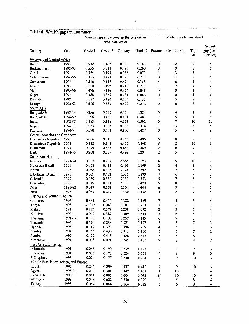
Table 4: Wealth gaps in attainmentWealth gaps (rich-poor) in the proportion Median grade completed

who completedWealth

Country Year Grade I Grade 5 Primary Grade 9 Bottom 40 Middle 40 Top gap (top -20 bottom)

Western and Central AfricaBenin 1993 0.532 0.462 0.383 0.162 0 2 5 5Burkina Faso 1992-93 0.556 0.514 0.490 0.200 0 0 6 6C.A.R. 1991 0.354 0.499 0.386 0.073 1 3 5 4Cote d'lvoire 1994-95 0.353 0.389 0.387 0.233 0 4 6 6Cameroon 1994 0.316 0.457 0.474 0.358 4 6 8 4Ghana 1993 0.150 0.197 0.210 0.273 7 7 9 2Mali 1995-96 0.476 0.436 0.374 0.041 0 0 4 4Niger 1992 0.388 0.355 0.281 0.086 0 0 4 4Rwanda 1992 0.117 0.180 0.224 0.155 4 5 6 2Senegal 1992-93 0.576 0.550 0.522 0.216 0 0 6 6South AsiaBangladesh 1993-94 0.386 0.520 0.520 0.384 0 4 8 8Bangladesh 1996-97 0.296 0.431 0.431 0.407 2 5 8 6India 1992-93 0.483 0.556 0.556 0.592 0 7 10 10Nepal 1996 0.233 0.338 0.338 0.314 3 3 8 5Pakistan 1990-91 0.570 0.602 0.602 0.487 0 5 9 9Central America and CaribbeanDominican Republic 1991 0.066 0.316 0.415 0.495 5 8 9 4Dominican Republic 1996 0.118 0.348 0.417 0.498 5 8 10 5Guatemala 1995 0.279 0.635 0.656 0.489 2 6 9 7Haiti 1994-95 0.208 0.529 0.498 0.291 2 5 6 4South AmericaBolivia 1993-94 0.032 0.232 0.565 0.573 6 9 10 4Northeast Brazil 1991 0.078 0.435 0.199 0.199 2 4 6 4Brazil 1996 0.068 0.438 0.426 0.302 4 7 8 4[Northeast Brazil] 1996 0.089 0.421 0.315 0.199 4 6 7 3Colombia 1990 0.039 0.330 0.330 0.353 5 7 8 3Colombia 1995 0.049 0.311 0.311 0.429 5 8 9 4Peru 1991-92 0.017 0.152 0.304 0.404 6 9 9 3Peru 1996 0.037 0.219 0.430 0.432 5 8 9 4Eastern end Southern AfricaComoros 1996 0.331 0.414 0.382 0.169 2 4 6 4Kenya 1993 -0.002 0.040 0.182 0.213 7 6 8 1Malawi 1992 0.223 0.372 0.238 0.092 2 3 6 4Namibia 1992 0.052 0.387 0.509 0.345 5 6 8 3Tanzania 1991-92 0.128 0.197 0.259 0.149 6 7 7 1Tanzania 1996 0.160 0.238 0.321 0.102 5 6 7 2Uganda 1995 0.147 0.377 0.396 0.219 4 5 7 3Zambia 1992 0.166 0.430 0.515 0.160 5 7 7 2Zambia 1992 0.137 0.418 0.526 0.315 5 6 8 3Zimbabwe 1994 0.015 0.071 0.245 0.461 7 8 9 2East Asia and PacificIndonesia 1991 0.046 0.190 0.239 0.475 6 8 9 3Indonesia 1994 0.036 0.173 0.224 0.501 6 8 9 3Philippines 1993 0.024 0.177 0.230 0.424 7 9 10 3Middle E]ast, North Africa, and EuropeEgypt 1992 0.245 0.299 0.337 0.410 7 9 10 3Egypt 1995-96 0.233 0.304 0.342 0.401 7 10 11 4Kazakhstan 1995 0.004 0.005 0.004 0.082 10 10 10 0Morocco 1992 0.548 0.622 0.630 0.390 0 5 8 8Turkey 1993 0.054 0.064 0.064 0.332 5 6 9 4

26

Table 4 reports the gap in the proportion of the 15 to 19 year old cohort who have

completed grade 1, grade 5, primary school, and grade 9. In Western/Central-Africa there are

large gaps at the primary level but by grade 9 attainment has fallen for the rich so the wealth

gap closes. In South Asia the wealth gap starts large and stays large ranging from .34 (Nepal)

to .60 (Pakistan) for primary school completion and from .31 (Nepal) to .59 (India) for grade

9 completion. In South America the wealth gap is less than .10 at grade 1, but gets

progressively larger. For example, by the end of primary school the wealth gap in completion

has reached .43 in Brazil, while in Bolivia by grade 9 it has reached .57. The wealth gaps in

the Eastern/Southern African countries are relatively small, even through primary completion

(except for Zambia and Uganda).

The second way of defining the wealth gap highlights striking differences across

countries. In the attainment profiles, the difference in median grade completed is the

horizontal gap at .5 (i.e. half the population).13 Figure 3 shows the median attainment of rich

and poor for each country. The last four columns of Table 4 report the median grade

attainment of the poor, middle and rich, as well as the difference between the rich and the

poor for each country. Perhaps not surprisingly, as countries move from low to high levels of

attainment, the gap starts out high, grows, peaks, and then falls when the entire population

enrolls and stays in school.

'3 This is calculated from the data and is not truncated at grade 9 as in the figures. This does imply that thedifferences are, if anything larger due to upper censoring of those still enrolled.

27

Grade

CDow J _ 3 w rs Oso 00 0 o

Niger 1992

Mali 1995-96

Benin 1993 Ls

i Burkina Faso 1992-93 Os

Cote dilvoire 1994 .I

qi Senegal 1992-93

(I, MoM ocF o 1992 _ ____oo _ _ ] _ O_

o Pakistan 1990-91 -*

India 1992-93

0. C-AR. 1994-95 _o

Bangladesh 1993-94 P.

Northeast Brazil 1991

Haiti 1994-95 _

Comoros 1996

Malawi 1992

Guatemala 1995o0D Bangladesh 1996-97 _.

Nepal 199611 111Rwanda 1992 =w

Uganda 19

Cameroon 1991 _ _ _ _ iI = X

Brazil 1996

Tanzania 1996 __

Zambia 1992 _

Zambia 1996-97 1

Colombia 1990 _ _

CP Namibia 1992

CD Dominican Republic 1991

o Dominican Republic 1996 _|

CD Colombia 1995 M0. Peru 1996 _ -

Turkel 1993 _ _ _ _- __

Tanzania 1991-92 =

C"o Ken;a 1993 -- - - -

Peru 1991-92

_. Indonesia 1991 w

Indonesia 1994 _

Bolivia 1993-94 __ __ ___

0~~~~~~~~~~~~~~~~~~~~~~

Q ~~Zimbabwe 19

Philippines 1993 __

Egypt 1992 ___

Egypt 1995-96 __

Kazakstan 1995 Co

In Western/Central Africa the median grade completed of the bottom 40 percent is

zero, as less than half of the poor in these countries ever finish even one year of schooling.

However, since the rich do not achieve very high levels of schooling either the wealth gap

ranges from 4 to 6 years.

The wealth gap is the highest in the world in South Asia where the poor are not going

to, nor staying in, school. The median grade completed is zero in all countries but Nepal (3

years) and Bangladesh in 1996-97 (2 years). However, the richer groups in these countries

have high levels of attainment. India has the world's largest gap of 10 years with the poor

having median grade completed of zero, while for the rich attainment is 10 years. This is

followed closely by Pakistan at 9 years, and Bangladesh in 1996-97 at 5.

The Latin American countries have smaller, but for their average attainment, enormous

wealth gaps. Haiti has a pattern similar to those in Western/Central Africa with median grade

completed of 2 for the poor and only 6 for the rich, while Guatemala has a pattern like that in

South Asia with a gap of 7 (2 for the poor versus 9 for the rich). The inequality in attainment

in South America results in a wealth gap of 4 years in all four countries with the median grade

completed ranging from 4 to 6 for the poor, and from 8 to 10 for the rich.

Again there is the striking comparison between Latin America and the much poorer

countries in Eastern/Southern Africa. The bottom 40 percent in Eastern/Southern Africa have

considerably higher educational attainment than the bottom 40 percent in Central or South

America. The median grade completed in Kenya, Ghana, and Zimbabwe is 7 in contrast to 4

in Brazil, and 5 in Colombia and Peru.

The Eastern/Southern African pattern of high initial enrollment and high retention of

all groups through primary leads to low wealth gaps ranging from 1 (Kenya) to 3 (Uganda and

Zambia). The wealth gap is equal to 3 for the two East Asian countries. This is due not to

especially low attainment for the poorest and middle groups, but rather to higher levels of

attainment of the richest group. The wealth gap in median grade completed is 4 in Egypt and

Turkey, again due largely to the high attainment of the richest group.

IV) ALttainment profiles as a diagnostic

The attainment profiles are also useful as a diagnostic as to where key concerns in the

systern are. When the issue of increasing enrollment rates or educational attainment is

discussed there is often a tendency to talk about "access" to schooling, where access is

narrowly defined as the physical availability of schools. This was almost certainly the key

issue some years ago when there just were not enough schools or teachers to go around.

However, it is increasingly unlikely that in many countries the physical presence or absence of

schools is a major constraint on expanding enrollment and attainment, particularly of the poor.

Many analysts have concluded that even in very poor countries improving the quality of

schooling is now the critical dimension for expanding enrollments. The figures presented here

provide three stylized facts that are consistent with this conjecture, two from the primary level

and o:ne from the transition from primary to secondary.

A) Primary

First, if a child went to school and then stopped going it is very likely that he or she

could have continued to go to school. The first column of Table 5 presents the proportion of

the shortfall in primary completion that is due to drop-out (i.e. the ratio of the difference

between grade 1 and primary completion and the shortfall in primary completion).

30

Table 5: Attainment and dropout ratesShortfall Proportion who completed Bottom 40 percent only,due to at least grade I simulated dropout rates

dropout, in the last between in theCountry Year bottom 40 All Top 20 rural year of primary second year

percent male primary secondary of secondary~~~~~~............... ..... .. .- ---.......... ......... ............. ........ -ec n m a le ..pr . .. ... ....i.....a...Western and Central AfricaBenin 1993 0.237 0.510 0.777 0.546 0.250 0.229Burkina Faso 1992-93 0.071 0.323 0.603 0.186 0.735 0.651C.A.R. 1991 0.490 0.686 0.946 0.684 0.629 0.506Cote dlvoire 1994-95 0.310 0.602 0.830 0.417 0.488 0.248Cameroon 1994 0.472 0.787 0.964 0.287 0.417 0.458Ghana 1993 0.399 0.830 1.000 0.060 0.128 0.165Mali 1995-96 0.097 0.294 0.484 0.461 0.509 0.259Niger 1992 0.140 0.250 0.412 0.862 0.169 0.037Rwanda 1992 0.683 0.786 0.826 0.444 0.746 0.538Senegal 1992-93 0.102 0.434 0.417 0.243 0.750 0.156South AsiaBangladesh 1993-94 0.307 0.666 0.881 0.215 0.437 0.231Bangladesh 1996-97 0.360 0.725 0.890 0.185 0.341 0.240India 1992-93 0.153 0.695 0.956 0.100 0.180 0.145Nepal 1996 0.317 0.632 0.894 0.173 0.206 0.212Pakistan 1990-91 0.104 0.577 0.936 0.111 0.331 0.192Central America and CaribbeanDominican Republic 1991 0.846 0.948 1.000 0.237 0.308 0.317Dominican Republic 1996 0.761 0.933 1.000 0.181 0.256 0.308Guatemala 1995 0.609 0.835 0.986 0.228 0.716 0.342Haiti 1994-95 0.694 0.848 0.824 0.387 0.482 0.397South AmericaBolivia 1993-94 0.940 0.981 1.000 0.239 0.323 0.449Northeast Brazil 1991 0.752 0.813 0.661 0.716 0.000 0.493Brazil 1996 0.911 0.962 1.000 0.321 0.476 0.496[Northeast Brazil] 1996 0.866 0.911 1.000 0.367 0.507 0.474Colombia 1990 0.863 0.967 0.741 0.168 0.407 0.270Colombia 1995 0.836 0.970 0.972 0.147 0.379 0.200Peru 1991-92 0.931 0.986 1.000 0.232 0.273 0.253Peru 1996 0.909 0.977 1.000 0.334 0.195 0.288Eastern and Southern AfricaComoros 1996 0.488 0.731 0.917 0.382 0.529 0.542Kenya 1993 0.923 0.956 0.943 0.269 0.461 0.637Malawi 1992 0.643 0.736 0.895 0.487 0.834 0.529Namibia 1992 0.894 0.933 0.773 0.390 0.430 0.628Tanzania 1991-92 0.652 0.872 0.921 0.189 0.985 0.415Tanzania 1996 0.685 0.865 0.952 0.219 0.980 0.424Uganda 1995 0.751 0.847 0.940 0.481 0.615 0.462Zambia 1992 0.757 0.909 0.925 0.367 0.856 0.791Zambia 1992 0.809 0.911 1.000 0.352 0.703 0.567Zimbabwe 1994 0.911 0.978 0.890 0.153 0.457 0.333East Asia and PacificIndonesia 1991 0.813 0.974 0.988 0.083 0.602 0.137Indonesia 1994 0.847 0.979 0.996 0.073 0.605 0.144Philippines 1993 0.898 0.987 0.996 0.083 0.240 0.177Middle East, North Africa, and EuropeEgypt 1992 0.342 0.842 0.984 0.105 0.082 0.079Egypt 1995-96 0.406 0.866 0.988 0.093 0.100 0.076Kazakhstan 1995 0.000 0.994 1.000 0.000 0.001 0.000Morocco 1992 0.291 0.652 1.000 0.499 0.295 0.262Turkey 1993 0.249 0.951 1.000 0.011 0.671 0.098

31

The striking results here are the high numbers for Latin America (60 to 94 percent),

EasternmSouthern Africa (excluding Ghana, 75 to 92 percent) and East Asia (85 and 90

percent),. In these countries, the main explanation for why children do not complete primary

school is not that they don't start school, it is the fact that they drop-out. In the

Western/Central African and South Asian countries, dropout explains less than half the

shortfall from universal primary education for the poor, with values ranging from 10 percent

in India to 49 percent in Comoros (which although it lies off the Eastern coast has the

attainment patterns of Western/Central Africa).

,Of course this approach can only address the question of the physical availability of

schools, not true access to education. In particular it is possible that children did attend first

grade, but in classes of 100 or more, with no materials, indifferent (or worse) teaching, and

deteriorating buildings. Not surprisingly there will be high drop-out, due not to physical

availability but to access to an education, which when properly defined, includes quality.

A second approach to the impact of school availability would be to look directly at the

relationship between the presence of schools and enrollment. For example, using the DHS

data from India, Filmer and Pritchett (1998b) found in state by state regressions that there was

only a weak relationship between the availability of schools and enrollment rates. In this

paper we don't replicate the analysis country by country but, as a heuristic indication, we

report the proportion of "Rich Rural Males" (RRM) who have completed at least grade 1.

Since poverty is not completely regionally concentrated this group is likely to suffer from a

similar lack of physical access to schools as less socially favored groups (the poor and

females). If RRM have high enrollment this provides some evidence on the degree to which

other groups are falling short due to their status, not school availability.

32

Table 5 shows large gaps in the low enrollment countries between rich rural males and

the average enrollment. In Pakistan RRM enrollment is 94 percent while the average is 58

percent (a 36 percentage point gap), in India RRM enrollment is 96 percent while average is

69 percent (a 37 percentage point gap), in Cote d'Ivoire RRM enrollment is 83 percent versus

60 percent (a 23 percentage point gap), and in C.A.R RRM enrollment is 95 percent versus

an average of 69 percent (a 36 percentage point gap). Expanding enrollment of the average to

that of RRM would nearly eliminate the proportion of children who completed less than 1 year

of schooling in most countries, except for the very lowest performers such as Mali or Benin.

B) Transition to secondary

The third point about availability is that the attainment profiles do not suggest that the

lack of availability of secondary schools, or rationing of secondary places, plays a large role in

most countries, although it is a central phenomenon in some. Table 5 reports the simulated

drop-out rate of the poor between the second-to-last and the last year of primary, between the

end of primary and the end of the first year of secondary, and between the first and second

years of secondary.' 4 If secondary school places were rationed (either officially by an exam or

in practice by the lack of facilities) one would expect to see the drop-out across the transition

between primary and secondary to be much larger than either before or after the transition

point.

This is indeed the pattern in some countries, identifiable graphically by a steep drop at

the end of the primary cycle. In Turkey the drop-out rate is 1.1 percent before the transition,

'4 Again, simulated as we are not observing the dropout behavior on an individual child, rather this is the valueimplied from the cross section of 15 to 19 year olds. For example, in a country in which the primary cycle is 6years, the simulated drop-out rate in the last year of primary is the ratio of the completion of grade 5 to thecompletion of grade 6, the rate between primary and secondary cycles is the ratio of the completion of grade 6 to the

33

67 percent across the transition, and 9.8 percent after it. In Tanzania the drop-out rate is 22

percent the year before, but 98 percent across the transition as almost no poor child made it to

secondary'5. High drop-out rates across the primary transition are also prominent in Indonesia

and Guatemala.

In nearly ever other country, however, drop-out is noticeably higher, but not

dramatically so, across the transition than in the year before or after. Most of the graphs are

characterized by very smooth slopes that make it difficult to distinguish visually which is the

transition year. For example, in Nepal the drop-out rate is 17 percent, 21 percent and 21

percent in the three years.

In the Philippines the drop-out rate is 8.3 before the end of primary, increases to 24

percent across the transition, and then falls slightly to 18 percent. This pattern of a higher rate

in the transition followed by a high, but lower, subsequent rate is true of Haiti, C.A.R.,

Zambia., and Uganda.

In the Dominican Republic the drop-out rate is 18 percent, 26 percent and 31 percent,

so drop-out is higher after the first year of secondary than in the transition before. This

pattern true of Bolivia and Brazil as well. The analysis reveals the importance of the entire

attainment profile. Looking only at average enrollment between primary and secondary one

might be tempted to conclude that the large gap indicated the problem was across the

transition. However, examining the profile might reveal that drop outs within primary imply

that the "excess" of primary school leavers over secondary entrants is quite low.

completion of grade 7, and the rate in the second year of secondary is the ratio between the completion of grade 7and the completion of grade 8.5 Keep in mind these are 15-19 year olds in the year of the survey and hence reflects the situation some years prior.

34

Figure 4 Figure 4 illustrates the

Brazil 1993 Indonesia 1994 point by showing the

> 0.8 < l 1 0.8 j average profiles for the

ao 0.6 ----- ----- . -. . 0.6 tpoorest 40 percent in

'; 0.4- ... ---- 0.4 - -;_ Brazil and Indonesia. In

0.2 - 0.2 - Brazil, dropout across

0o -0 l the transition may be1 2 3 4 5 6 7 89 1 2 3 4 5 6 7 8 9

Grade Gradehigh (48 percent), but it

_ Poorest n Middle A Richestis high all throughout

the primary school years. In Indonesia, dropout is ten percentage points higher across the

transition (61 percent) but the underlying profile is vastly different as there is a very small

amount of dropout within the primary school years and virtually all of the drop-off is across

the transition.

Of course this use of the attaimnent profile is diagnostic and can only point to issues

for more detailed examination. For instance Lavy (1997) has shown that the lack of secondary

school facilities can influence drop-out at the primary levels even before the end of primary by

lowering the expected return to additional primary years. Therefore, we cannot conclude from

high primary drop-out that the physical lack of secondary facilities is not an important issue.

35

Conclusion

In this paper we have documented striking cross-country patterns in education

enrollment and attainment in 35 countries.

While many others have examined the differences in enrollment rate behavior between

the rich and poor, a major advantage of this analysis is that the data are comparable. The

attainment data are derived consistently and, while the levels of the asset index are not directly

comparable across countries, they are derived using an identical methodology.

There are two overall conclusions that emerges from these results. First, many (if not

most) countries the bulk of the deficit from universal enrollment up to primary (or basic)

comes from the poor. The achievement of higher levels of enrollment for this group is an

exercise in social inclusion, reaching out and bringing the poorest into what is already the

norm for the rich and, in many cases, the middle class. Second, the evidence suggests that,

except in the very poorest settings, the key to closing wealth gaps in enrollment and attainment

will require actions which raise the demand for schooling of the poor. Raising the quality of

schooling received at the primary level is likely to be the key ingredient to attract and retain

poor children in school.

36

References

Ahuja, Vinod and Deon Filmer, 1996 "Educational Attainment in Developing Countries: NewEstimates and Projections Disaggregated by Gender". Journal of Educational Planning andAdministration Vol X(3):229-254.

Barro, Robert and Jong-Wha Lee, 1993. "International Comparisons of EducationalAttainment," Journal of Monetary Economics, 32:363-394.

Behrman, Jere R. and James C. Knowles, 1997. "How Strongly is Child Schooling Associatedwith Household Income?" University of Pennsylvania and Abt Associates. Mimeo.

Castro-Leal, Florencio, Julia Dayton, Lionel Demery, and Kalpana Mehra, 1997, "Public socialspending in Africa: do the poor benefit?" mimeo, PRMPO, The World Bank.

Dubey, Ashutosh and Elizabeth King. 1994. "A New Cross-Country Education Stock SeriesDifferentiated by Age and Sex", mimeo, The World Bank

Filmer, Deon and Lant Pritchett, 1998a. "Estimating wealth effects without income ofexpenditure data -- or tears: Educational enrollment in India," mimeo, DECRG, The WorldBank. Washington, DC.

Filmer, Deon and Lant Pritchett, 1998b, "Determinants of Education Enrollment in India:Child, Household, Village and State Effects," mimeo, DECRG, The World Bank. Washington,DC.

Hammer, Jeffrey, 1998. "Health Outcomes across wealth groups in Brazil and India," mimeo,DECRG, The World Bank. Washington, DC.

Lavy, Victor. 1997. "School supply constraints and children's educational outcomes in ruralGhana," Journal of Development Economics, 51:[291]-314.

Montgomery, Mark, Kathleen Burke, Edmundo Paredes, and Salman Zaidi, 1997. "MeasuringLiving Standards with DHS Data: Any Reason to Worry?" mimeo, Research Division, ThePopulation Council. New York, NY.

Nehru, Vikram, Eric Swanson and Ashutosh Dubey, 1993. "New Database on Human CapitalStock in Developing and Industrial Countries: Sources, Methodology, and Results," Journal ofDevelopment Economics, 46:379-401

Patrinos, Harry Anthony. 1997. "Differences in Education and Earnings Across Ethnic Groupsin Guatemala," Quarterly Review of Economics and Finance 37:809-821.

37

Table A-1: Proportion who have completed grade or higherBottom 40 percent Middle 40 percent lop 20 percent

Year Grade I Grade 5 Primary Grade 9 Grade I Grade 5 Primary Grade 9 Grade I Grade 5 Primnary Grade 9W estern and Central A frica ~ ~ ~ ......... ...... .. --- - -- ----........................ .................... ..... ...- .......

Bcnin 1993 0.264 0.079 0.036 0.007 0.530 0.312 0.203 0.043 0.797 0.541 0,419 0.169Burkina Fasu 1992-93 0.130 0.00788 0.064 0.002 0.2,52 0.I7 80. 1 50 0.023 0.686 0.5920.553 0,203C.AR. 1991 0.514 0.148 0.047 0.003 0.729 0.367 0.206 0.037 0.868 0.647 0.433 0.076Cote dIlvoire 1994-95 0.419 0.271 0.158 0.039 0.635 0.447 0.311 0.115 0.772 0.660 0.545 0.272Camneroon 1994 0.640 0.446 0,318 0.055 0.819 0.685 0.540 0.156 0.956 0.903 0.792 0,413Ghana 1993 0.791 0.694 0.652 0.306 0.799 0.714 0.666 0.319 0.941 0.891 0.862 0.579Mali 1995-96 0.119 0.046 0.025 0.001 0.248 0.139 0.100 0.006 0.595 0.482 0.399 0.043Niger 1992 0.154 0.113 0.016 0.007 0.175 0.129 0.032 0.011 0.541 0.468 0.297 0.093Rwanda 1992 0.730 0.469 0.147 0.037 0.802 0.552 0.199 0.067 0.846 0.649 0.371 0.192Senegal 1992-93 0.199 0.143 0.108 0.017 0.454 0.367 0.301 0.057 0.776 0,693 0.630 0.232South AsiaBangladesh 1993-94 0.497 0.274 0.274 0.063 0.682 0.464 0.464 0.148 0.883 0.794 0.794 0.447Bangladesh 1996-97 0.588 0.356 0.356 0.080 0.755 0.550 0.550 0.i74 0.885 0.788 0.788 0.487India 1992-93 0.472 0.376 0.376 0.139 0.761 0.684 0.684 0.363 0.954 0.932 0.932 0.730Nepal 1996 0.594 0.406 0.406 0.116 0.551 0.414 0.414 0.139 0.827 0.743 0.743 0.430Pakistan 1990-91 0.328 0.250 0.250 0.065 0.614 0.522 0.522 0.209 0.898 0.852 0.852 0.552Central America and CaribbeanDominican Republic 1991 0.912 0.560 0.427 0.111 0.967 0.828 0.734 0.399 0.978 0.876 0.843 0.606Dominican Republic 1996 0.873 0.569 0.466 0.143 0.962 0.831 0.760 0.402 0.991 0.917 0.883 0.641Guatemala 1995 0.680 0.236 0.182 0.022 0.894 0.632 0.557 0.181 0.959 0.871 0.839 0.511Haiti 1994-95 0.724 0.161 0.099 0.018 0.894 0.512 0.363 0.105 0.932 0.690 0.597 0.308South AmericaBolivia 1993-94 0.958 0.705 0.288 0.195 0.995 0.927 0.716 0.588 0.989 0.937 0.853 0.768Northeast Brazil 1991 0.754 0.121 0.009 0.009 0.855 0.438 0.074 0.074 0.832 0.556 0.208 0.208Brazil 1996 0.924 0.457 0.150 0.078 0.986 0.801 0.449 0.277 0.992 0.895 0.576 0.381[Northeast Brazil] 1996 0.879 0.344 0.093 0.046 0.968 0.721 0.358 0.223 0.967 0.766 0.408 0.245Colombia 1990 0.941 0.571 0,571 0.096 0.983 0.870 0.870 0.321 0.980 0.902 0.902 0.449Colombia 1995 0.939 0.630 0.630 0.145 0.989 0.906 0.906 0.443 0.989 0.942 0.942 0.574Peru 1991-92 0.974 0.813 0.624 0.217 0.993 0.963 0.907 0.502 0.991 0.965 0.928 0.621Peru 1996 0.954 0.746 0.496 0.175 0.988 0.951 0.879 0.462 0.991 0.964 0.926 0.608Eastern and Southern AfricaComoros 1996 0.576 0.280 0.173 0.014 0.762 0.475 0.299 0.059 0.907 0.694 0.555 0.183Kenya 1993 0.963 0.835 0.520 0.102 0.946 0.801 0.463 0.103 0.961 0.85 0.702 0.315Malawi 1992 0.666 0.291 0.066 0.011 0.715 0.393 0.106 0.014 0.889 0.664 0.304 0. 103Natnibia 1992 0.918 0.528 0.223 0.047 0.933 0.657 0.355 0.122 0.970 0.915 0.732 0.392Tanzania 1991-92 0.821 0.676 0.486 0.004 0.876 0.736 0.548 0.023 0.949 0.873 0.744 0.153Tanzania 1996 0.803 0.618 0.376 0.004 0.861 0.665 0.406 0.014 0.964 0.857 0.697 0.107Uganda 1995 0.784 0.390 0.130 0.027 0.871 0.533 0.215 0.060 0.930 0.767 0.525 0.246Zamnbia 1992 0.819 0.524 0.255 0.008 0.946 0.816 0.540 0.038 0.985 0.954 0.770 0.168Zambia 1992 0.858 0.537 0.254 0.033 0.909 0.711 0.445 0.100 0.995 0.955 0.779 0.347Zimbabwe 1994 0.973 0.892 0.696 0.252 0.979 0.930 0.794 0.397 0.988 0.963 0.941 0.713East Asia and PacificIndonesia 1991 0.946 0.778 0.713 0.186 0.987 0.905 0.869 0.423 0.993 0.967 0.952 0.661Indonesia 1994 0.959 0.787 0.730 0.190 0.987 0.916 0.884 0.445 0.995 0.960 0.953 0.691Philippines 1993 0.973 0.801 0.735 0.320 0.992 0.954 0.933 0.618 0.997 0.978 0.965 0.744Middle East, North Africa, and EuropeEgypt 1992 0.718 0.639 0.571 0.374 0.907 0.857 0.792 0.565 0.963 0.938 0.909 0.784Egypt 1995-96 0.745 0.631 0.572 0.396 0.927 0.845 0.799 0.628 0.978 0.935 0.913 0.798Kazakhstan 1995 0.995 0.994 0.995 0.833 0.991 0.989 0.989 0.883 0.999 0.999 0.999 0.915Morocco 1992 0.366 0.211 0,106 0.029 0.777 0.601 0.426 0.164 0.914 0.833 0.735 0.419Turkey 1993 0.932 0.910 0.910 0.186 0.953 0.933 0.933 0.372 0.986 0.974 0.974 0.5 17

38

Policy Research Working Paper Series

ContactTitle Author Date for paper

WPS1965 Manufacturing Firms in Developing James Tybout August 1998 L. TabadaCountries: How Well Do They Do, 36869and Why

WPS196E Sulfur Dioxide Control by Electric Curtis Carlson August 1998 T. TourouguiUtilities: What Are the Gains from Dallas Burtraw 87431Trade? Maureen Cropper

Karen L. Palmer

WPS196J Agriculture and the Macroeconomy Maurice Schiff August 1998 A. Vald6sAlberto Valdes 35491

WPS1968 The Economics and Law of Rent Kaushik Basu August 1998 M. MasonControl Patrick Emerson 30809

WPS1 969 Protecting the Poor in Vietnam's Dominique van de Walle September 1998 C. BernardoEmerging Market Economy 31148

WPS197IJ Trade Liberalization and Endogenous Thomas F. Rutherford September 1998 L. TabadaGrowth in a Small Open Economy: David G. Tarr 36896A Quantitative Assessment

WPS1971 Promoting Better Logging Practices Marco Boscolo September 1998 T. Tourouguiin Tropical Forests Jeffrey R. Vincent 87431

WPS1972 Why Privatize? The Case of Geroge R. G. Clarke September 1998 P. Sintim-AboagyeArgentina's Public Provincial Banks Robert Cull 38526

WPS1973 The Economic Analysis of Sector Sethaput Suthiwart- September 1998 C. BernardoInvestment Programs Narueput 31148

WPS1974 Volatility and the Welfare Costs Pierre-Richard Agenor September 1998 S. King-Watsonof Financial Market Integration Joshua Aizenman 33730

WPS1 975 Acting Globaily While Thinking Gunnar S. Eskeland September 1998 C. BernardoLocally: Is the Global Environment Jian Xie 31148Protected by Transport EmissionControl Programs

WPS1976 Capital Flows to Central and Stijn Claessens September 1998 R. VoEastern Europe and the Former Daniel Oks 33722Soviet Union Rossana Polastri

WPS1977 Economic Reforms in Egypt: Rania A. Al-Mashat September 1998 S. DyEmerging Patterns and Their David A. Grigorian 32544Possible Implications

WPS19'78 Behavioral Responses to Risk Jyotsna Jalan September 1998 P. Saderin Rural China Martin Ravallion 33902

Policy Research Working Paper Series

ContactTitle Author Date for paper

WPS1979 Banking on Crises: Expensive Gerard Caprio, Jr. September 1998 P. Sintim-AboagyeLessons from Recent Financial 38526Crises