
The copyright © of this thesis belongs to its rightful...
346
The copyright © of this thesis belongs to its rightful author and/or other copyright owner. Copies can be accessed and downloaded for non-commercial or learning purposes without any charge and permission. The thesis cannot be reproduced or quoted as a whole without the permission from its rightful owner. No alteration or changes in format is allowed without permission from its rightful owner.
Transcript of The copyright © of this thesis belongs to its rightful...

The copyright © of this thesis belongs to its rightful author and/or other copyright
owner. Copies can be accessed and downloaded for non-commercial or learning
purposes without any charge and permission. The thesis cannot be reproduced or
quoted as a whole without the permission from its rightful owner. No alteration or
changes in format is allowed without permission from its rightful owner.

IMPACT OF FOREIGN CAPITAL INFLOWS ON
ECONOMIC GROWTH IN THE PRESENCE OF
CURRENCY AND BANKING CRISES
SYED ALI RAZA
DOCTOR OF PHILOSOPHY
UNIVERSITI UTARA MALAYSIA
January 2017

i
IMPACT OF FOREIGN CAPITAL INFLOWS ON ECONOMIC GROWTH IN
THE PRESENCE OF CURRENCY AND BANKING CRISES
By
SYED ALI RAZA
Thesis Submitted to
Othman Yeop Abdullah Graduate School of Business,
Universiti Utara Malaysia,
in Fulfillment of the Requirement for the Degree of Doctor of Philosophy


iv
PERMISSION TO USE
In presenting this thesis in fulfilment of the requirements for a postgraduate degree from
Universiti Utara Malaysia, I agree that the Universiti Library may make it freely
available for inspection. I further agree that permission for the copying of this thesis in
any manner, in whole or in part, for scholarly purpose may be granted by my
supervisor(s) or, in their absence, by the Dean of Othman Yeop Abdullah Graduate
School of Business. It is understood that any copying or publication or use of this thesis
or parts thereof for financial gain shall not be allowed without my written permission. It
is also understood that due recognition shall be given to me and to Universiti Utara
Malaysia for any scholarly use which may be made of any material from my thesis.
Requests for permission to copy or to make other use of materials in this thesis, in whole
or in part, should be addressed to:
Dean of Othman Yeop Abdullah Graduate School of Business
Universiti Utara Malaysia
06010 UUM Sintok
Kedah Darul Aman

v
ABSTRACT
Foreign capital inflows (FCI) have been considered to be a key element in the process of
economic globalization and integration of the world economy. However, the frequent
occurrence of financial crises around the world has awakened the debate about the
causes, consequences, impact and aftershocks of these crises. These sorts of financial
crises are majorly occurring because of systemic banking crisis and currency crisis.
These crises significantly influence the relationship between FCI and economic growth.
The objective of this study is to identify the impact of foreign direct investment, foreign
debt, workers‘ remittances and exports of goods and services on economic growth in
high, upper middle, lower middle and low income countries. To attain the objective of
this research, we collect a panel data of 96 countries and group them on the basis of
different income levels. The final sample of this study consists of 10 low income
countries, 23 lower middle income countries, 30 upper middle income countries and 33
high income countries. We employed fixed effect & random effect model estimation
method to judge the desired relationship among variables. Fully modified ordinary least
squares (FMOLS) has also been used to ensure the robustness of initial results. Results
indicate the negative and significant influence of systemic banking and currency crisis.
Results also indicate the positive and significant impact of all four types of FCI on
economic growth in all income level countries except, remittances in low income
countries and foreign debt in lower middle income. These two results show the negative
impact on economic growth. Results also conclude that the banking and currency crisis
are harmful for the relationship of foreign direct investment and economic growth in all
income level countries. The study recommends several policy implications to improve
the positive impact of foreign capital inflows on economic growth and reduce or control
the negatively influence of systemic banking crisis and currency crisis on the
relationship of foreign capital inflows and economic growth.
Keywords: systemic banking crisis, currency crisis, foreign capital inflows, economic
growth

vi
ABSTRAK
Aliran masuk modal telah dikatakan sebagai satu elemen penting dalam proses
globalisasi dan integrasi ekonomi dunia. Bagaimanapun, krisis ekonomi yang sering
berlaku diseluruh dunia telah menimbulkan perdebatan tentang sebab, akibat, impak dan
kejutan selepas krisis ini. Krisis kewangan seperti ini kebanyakkanya berlaku
disebabkan krisis sistemik perbankan dan krisis mata wang. Krisis-krisis ini secara
signifikan mempengaruhi perhubungan antara aliran masuk modal dan pertumbuhan
ekonomi. Objektif kajian ini ialah untuk mengenalpasti kesan pelaburan luar langsung,
hutang luar negara, kiriman wang pekerja, dan ekspot barangan dan perkhidmatan
keatas pertumbuhan ekonomi di negara-negara berpendapatan tinggi, pertengahan atas,
pertengahan bawah dan rendah. Bagi mencapai objektif kajian, data panel dari 96 buah
negara dikumpul dan di kelaskan mengikut tingkat pendapatan yang berbeza. Sampel
terakhir mengandungi 10 negara berpendapatan rendah, 23 negara berpendapatan
pertengahan bawah, 30 negara berpendapatan pertengahan atas dan 33 negara
berpendapatan tinggi. Kaedah model penganggaran kesan tetap dan kesan rawak
digunakan untk menentukan perhubungan yang diingini antara pembolehubah. Kaedah
Fully modified ordinary least squares (FMOLS) juga digunakan bagi memastikan
keputusan awal yang kukuh. Keputusan penganggaran menunjukkan kesan negatif dan
signifikan krisis sistemik perbankan dan krisis matawang. Keputusan kajian juga
menunjukkan kesan yang positif dan signifikan kesemua empat jenis aliran masuk
modal keatas pertumbuhan ekonomi negara disemua tingkat pendapatan kecuali kiriman
wang di negara berpendapatan rendah dan hutang luar negara di negara berpendapatan
pertengahan bawah. Kedua-dua keputusan tersebut menunjukkan impak yang negatif ke
atas pertumbuhan ekonomi. Keputusan juga menyimpulkan bahawa krisis perbankan
dan krisis mata wang adalah memudaratkan kepada hubungan antara pelaburan luar
langsung dan pertumbuhan ekonomi negara di semua tingkat pendapatan. Kajian ini
mencadangkan beberapa implikasi ekonomi bagi memperbaiki impak positif aliran
masuk modal ke atas pertumbuhan ekonomi dan mengurangkan atau mengawal
pengaruh negatif krisis sistemik perbankan dan krisis matawang ke atas hubungan
antara aliran masuk modal dan pertumbuhan ekonomi.
Kata kunci: krisis sistemik perbankan, krisis mata wang, aliran masuk modal,
pertumbuhan ekonomi

vii
ACKNOWLEDGEMENT
I thank Allah (SWT) who has made it possible for me to successfully complete my
Doctor of Philosophy programme. I would also like to express my sincere appreciation
to my supervisor Professor Dr. Mohd Zaini Abd Karim for his guidance towards the
successful completion of this thesis. I equally thank him for his encouragement and
kindness, all of which have made me to learn so much from him.
My gratitude goes to the members of the proposal defence committee, Professor Dr.
Jauhari Dahalan and Associate Professor Dr. Hussin Abdullah for their useful
contribution. My sincere appreciation goes to my family members: Syed Safir ul
Hassan, Kauser Sultana, Syeda Kanwal Hassan, Kanza Khan, Syeda Javeria Hassan and
Syed Ahmed Raza for their support and prayers, while they endured my continued
absence during my study in Malaysia. I am indebted to them for their understanding,
love and appreciations during my study.
I would like to register my appreciation to Dr. Wasim Qazi and Mr. Imtiaz Arif for their
continuance support. I would also like to express my sincere appreciation to my first
research mentor Mr. Syed Tehseen Jawaid. I would also like to convey my great thanks
to my colleagues and friends Arsalan Najmi, Muhammad Ali, Nida Shah, Amna Umer
and Muhammad Asif Qureshi
Last but not least, my sincere appreciation goes out to all those involved in making this
thesis a reality and those who have contributed towards this profound learning
experience.
viii
TABLE OF CONTENTS
TITLE PAGE ................................................................................................................................. I
CERTIFICATION OF THESIS WORK ................................................................................... II
CERTIFICATION OF THESIS WORK ................................................................................. III
PERMISSION TO USE .............................................................................................................. IV
ABSTRACT .................................................................................................................................. V
ABSTRAK ................................................................................................................................... VI
ACKNOWLEDGEMENT ........................................................................................................ VII
TABLE OF CONTENTS ......................................................................................................... VIII
LIST OF TABLES ....................................................................................................................... X
LIST OF FIGURES .................................................................................................................. XII
LIST OF ABBREVIATIONS ................................................................................................. XIII
CHAPTER ONE INTRODUCTION .......................................................................................... 1
1.1 Introduction ............................................................................................................ 1
1.2 Background of the Study ........................................................................................ 1
1.3 Problem Statement ................................................................................................ 27
1.4 Research Questions............................................................................................... 34
1.5 Objective(s) of the Study ...................................................................................... 34
1.6 Justification and Contribution of the Study .......................................................... 35
1.7 Scope of the Study ................................................................................................ 38
1.8 Plan of the Study................................................................................................... 39
1.9 Summary of the Chapter ....................................................................................... 39
CHAPTER TWO LITERATURE REVIEW ........................................................................... 41
2.1 Introduction ........................................................................................................... 41
2.2 Theoretical background ......................................................................................... 41
2.2.1 Theories of Economic Growth ........................................................................ 41
2.2.2 Foreign Direct Investment and Economic Growth ......................................... 51
2.2.3 Foreign Debt and Economic Growth .............................................................. 60
2.2.4 Workers‘ Remittances and Economic Growth ............................................... 67
2.2.5 Exports and Economic Growth ....................................................................... 71
2.3 Empirical Studies .................................................................................................. 93
2.3.1 Foreign Capital Inflows and Banking & Currency Crises .............................. 93
2.3.2 Foreign Direct Investment and Economic Growth ....................................... 101
2.3.3 Foreign Debt and Economic Growth ............................................................ 110
2.3.4 Workers‘ Remittances and Economic Growth ............................................. 116
2.3.5 Exports and Economic Growth ..................................................................... 125
2.4 Research Gap ....................................................................................................... 135
CHAPTER THREE THEORETICAL FRAMEWORK AND RESEARCH
METHODOLOGY .................................................................................................................... 138
3.1 Introduction ......................................................................................................... 138
3.2 Theoretical Framework ....................................................................................... 138
3.3 Methodology ....................................................................................................... 145

ix
3.4 Model Specification ............................................................................................ 147
3.5 Estimation of the Procedure ............................................................................... 154
3.5.1 Panel Unit Root and Co-Integration Test ..................................................... 155
3.5.2 Fixed Effects Model...................................................................................... 155
3.5.3 Random Effects Model ................................................................................. 157
3.6 Description of Variables ...................................................................................... 159
3.7 Research Hypothesis ........................................................................................... 163
3.8 Sources of Data ................................................................................................... 164
3.9 Summary of Chapter ........................................................................................... 166
CHAPTER FOUR RESULTS AND DISCUSSION .............................................................. 167
4.1 Introduction ......................................................................................................... 167
4.2 Descriptive Statistics ........................................................................................... 167
4.3 Low Income Countries ........................................................................................ 177
4.3.1 Unit Root Analyses ....................................................................................... 177
4.3.2 Cointegration Analyses ................................................................................. 178
4.3.3 Long Run Analysis ....................................................................................... 182
4.4 Lower Middle Income Countries......................................................................... 193
4.4.1 Unit Root Analyses ....................................................................................... 193
4.4.2 Cointegration Analyses ................................................................................. 194
4.4.3 Long Run Analysis ....................................................................................... 198
4.5 Upper Middle Income Countries ......................................................................... 209
4.5.1 Unit Root Analyses ....................................................................................... 209
4.5.2 Cointegration Analyses ................................................................................. 210
4.5.3 Long Run Analysis ....................................................................................... 214
4.6 High Income Countries........................................................................................ 224
4.6.1 Unit Root Analyses ....................................................................................... 224
4.6.2 Cointegration Analyses ................................................................................. 225
4.6.3 Long Run Analysis ....................................................................................... 229
4.7 Aggregate Results of 96 Countries ...................................................................... 237
4.7.1 Unit Root Analyses ....................................................................................... 237
4.7.2 Cointegration Analyses ................................................................................. 238
4.7.3 Long Run Analysis ....................................................................................... 242
4.8 Fully Modified Ordinary Least Square ............................................................... 253
4.9 Discussion of Result ............................................................................................ 261
4.10 Summary of Chapter.......................................................................................... 268
CHAPTER FIVE SUMMARY OF MAJOR FINDINGS, CONCLUSION AND
POLICY IMPLICATIONS ...................................................................................................... 270
5.1 Introduction ......................................................................................................... 270
5.2 Summary of Major Findings & Conclusion ........................................................ 270
5.3 Policy Implications .............................................................................................. 274
5.4 Limitations of the Study ...................................................................................... 279
5.5 Recommendations for Future Research .............................................................. 281
REFERENCES .......................................................................................................................... 282

x
LIST OF TABLES
Table 3.1: List of 96 Low, Lower Middle, Upper Middle and High Income Countries ............ 165
Table 4.1: Summary Statistics for Variables of Low Income Countries .................................... 168
Table 4.2: Summary Statistics for Variables of Lower Middle Income Countries ..................... 170
Table 4.3: Summary Statistics for Variables of Upper Middle Income Countries ..................... 172
Table 4.4: Summary Statistics for Variables of High Income Countries .................................... 173
Table 4.6: Results of Stationary Analyses for Low Income Countries ....................................... 177
Table 4.7: Results of Pedroni ((Engle-Granger based) Panel Cointegration in Low
Income Countries ........................................................................................................................ 179
Table 4.8: Results of Pedroni ((Engle-Granger based) Panel Cointegration of Interaction
Terms in Low Income Countries................................................................................................. 180
Table 4.9: Results of Kao (Engle-Granger based) Panel Cointegration in Low Income
Countries ..................................................................................................................................... 181
Table 4.10: Long Run Results of Banking and Currency Crisis in Low Income Countries ....... 184
Table 4.11: Long Run Results of Foreign Direct Investment in Low Income Countries ........... 186
Table 4.12: Long Run Results of Exports in Low Income Countries ......................................... 188
Table 4.13: Long Run Results of Remittances in Low Income Countries.................................. 190
Table 4.14: Long Run Results of External Debt in Low Income Countries ............................... 192
Table 4.15: Results of Stationary Analyses for Lower Middle Income Countries ..................... 193
Table 4.16: Results of Pedroni ((Engle-Granger based) Panel Cointegration in Lower
Middle Income Countries ............................................................................................................ 195
Table 4.17: Results of Pedroni ((Engle-Granger based) Panel Cointegration of
Interaction Terms in Lower Middle Income Countries............................................................... 196
Table 4.18: Results of Kao (Engle-Granger based) Panel Cointegration in Lower Middle
Income Countries ........................................................................................................................ 197
Table 4.19: Long Run Results of Banking and Currency Crisis in Lower Middle Income
Countries ..................................................................................................................................... 199
Table 4.20: Long Run Results of Foreign Direct Investment in Lower Middle Income
Countries ..................................................................................................................................... 201
Table 4.21: Long Run Results of Exports in Lower Middle Income Countries ......................... 203
Table 4.22: Long Run Results of Remittances in Lower Middle Income Countries .................. 206
Table 4.23: Long Run Results of External Debt in Lower Middle Income Countries ............... 208
Table 4.24: Results of Stationary Analyses for Upper Middle Income Countries...................... 209
Table 4.25: Results of Pedroni ((Engle-Granger based) Panel Cointegration in Upper
Middle Income Countries ............................................................................................................ 210
Table 4.26: Results of Pedroni ((Engle-Granger based) Panel Cointegration of
Interaction Terms in Upper Middle Income Countries ............................................................... 212
Table 4.27: Results of Kao (Engle-Granger based) Panel Cointegration in Upper Middle
Income Countries ........................................................................................................................ 213
Table 4.28: Long Run Results of Banking and Currency Crisis in Upper Middle Income
Countries ..................................................................................................................................... 215
Table 4.29: Long Run Results of Foreign Direct Investment in Upper Middle Income
Countries ..................................................................................................................................... 217
Table 4.30: Long Run Results of Exports in Upper Middle Income Countries .......................... 219

xi
Table 4.31: Long Run Results of Remittances in Upper Middle Income Countries .................. 221
Table 4.32: Long Run Results of External Debt in Upper Middle Income Countries ................ 223
Table 4.33: Results of Stationary Analyses for High Income Countries .................................... 224
Table 4.34: Results of Pedroni ((Engle-Granger based) Panel Cointegration in High
Income Countries ........................................................................................................................ 226
Table 4.35: Results of Pedroni ((Engle-Granger based) Panel Cointegration of
Interaction Terms in High Income Countries.............................................................................. 227
Table 4.36: Results of Kao (Engle-Granger based) Panel Cointegration in High Income
Countries ..................................................................................................................................... 228
Table 4.37: Long Run Results of Banking and Currency Crisis in High Income
Countries ..................................................................................................................................... 230
Table 4.38: Long Run Results of Foreign Direct Investment in High Income Countries .......... 232
Table 4.39: Long Run Results of Exports in High Income Countries ........................................ 234
Table 4.40: Long Run Results of Remittances in High Income Countries ................................. 236
Table 4.41: Results of Stationary Analyses for Upper Middle Income Countries...................... 237
Table 4.42: Results of Pedroni ((Engle-Granger based) Panel Cointegration in
Aggregate Sample of 96 Countries ............................................................................................. 239
Table 4.43: Results of Pedroni ((Engle-Granger based) Panel Cointegration of
Interaction Terms in Aggregate Sample of 96 Countries............................................................ 240
Table 4.44: Results of Kao (Engle-Granger based) Panel Cointegration in Aggregate
Sample of 96 Countries ............................................................................................................... 241
Table 4.45: Long Run Results of Banking and Currency Crisis in Aggregate Sample of
96 Countries ................................................................................................................................ 243
Table 4.46: Long Run Results of Foreign Direct Investment in Aggregate Sample of 96
Countries ..................................................................................................................................... 246
Table 4.47: Long Run Results of Exports in Aggregate Sample of 96 Countries ...................... 248
Table 4.48: Long Run Results of Remittances in Aggregate Sample of 96 Countries ............... 250
Table 4.49: Long Run Results of External Debt in Aggregate Sample of 96 Countries ............ 252
Table 4.50: Results of FMOLS in Low Income Countries ......................................................... 254
Table 4.51: Results of FMOLS in Low Income Countries ......................................................... 254
Table 4.52: Results of FMOLS in Lower Middle Income Countries ......................................... 255
Table 4.53: Results of FMOLS in Lower Middle Income Countries ......................................... 256
Table 4.54: Results of FMOLS in Upper Middle Income Countries .......................................... 257
Table 4.55: Results of FMOLS in Upper Middle Income Countries .......................................... 257
Table 4.56: Results of FMOLS in High Income Countries ........................................................ 258
Table 4.57: Results of FMOLS in High Income Countries ........................................................ 259
Table 4.58: Results of FMOLS in in Aggregate Sample of 96 Countries .................................. 260
Table 4.59: Results of FMOLS in in Aggregate Sample of 96 Countries .................................. 260
Table 4.60: Summary of Estimation Results of all Countries ..................................................... 262

xii
LIST OF FIGURES
Figure 1.1 Exports of goods and services as % of gdp for different income level
countries ........................................................................................................................................ 21 Figure 1.2 Exports of goods and services (annual growth) for different income level
countries ........................................................................................................................................ 22 Figure 1.3 Foreign direct investment as % of gdp for different income level countries............... 22 Figure 1.4 Foreign direct investment (annual growth) for different income level
countries ........................................................................................................................................ 23 Figure 1.5 Workers‘ remittances as % of gdp for different income level countries ..................... 24
Figure 1.6 Workers‘ remittances (annual growth) for different income level countries .............. 25
Figure 1.7 External debt (annual growth) for different income level countries ............................ 26
Figure 1.8 Gross domestic product (annual growth) for different income level countries ........... 26 Figure 2.1 Graphical representation of the laffer curve for debt relief ......................................... 66 Figure 3.1 Conceptual framework of the study ........................................................................... 145

xiii
LIST OF ABBREVIATIONS
FCI – Foreign Capital Inflows
EG – Economic Growth
FDI – Foreign Direct Investment
EXP – Exports of Goods and Services
ED – External Debt
EXD – External Debt
FD – Foreign Debt
REM – Workers‘ Remittances
CRC – Currency Crises
BAC – Banking Crises
FC – Financial Crises
SSE – Secondary School Enrollment
INF – Inflation (Consumer Price Index)
GCE – Government Consumption Expenditure
DOC – Domestic Credit provided by financial sector
FE – Fixed Effect Model
RE – Random Effect Model
FMOLS – Fully Modified Ordinary Least Square
GNI – Gross National Income
MNCs – Multi National Corporations
GDP – Gross Domestic Product
IMF – International Monetary Funds
WDI – World Development Indicators
IPS – Im, Pesaran & Shin
PP - Phillips and Perron
ADF - Augmented Dickey Fuller
VIF - Variance Inflation factor
OLS - Ordinary Least Square
LI – Low Income
LMI – Lower Middle Income
UMI – Upper Middle Income
HI – High Income

1
CHAPTER ONE
INTRODUCTION
1.1 Introduction
This chapter shed some light on the background information related to the foreign
capital inflows, systemic banking crisis, currency crisis and economic growth. This is
followed by statement of problem where the influence of financial crises on the
relationship of foreign capital inflows and economic is discussed. This chapter also
presents the research questions, research objectives, justification and contribution of the
study, scope of study, and the organization of the study.
1.2 Background of the Study
Foreign capital inflows play a significant role in the economic growth of both
developing and developed countries (Raza & Jawaid, 2014). Foreign capital has also
been considered to be a key element in the process of economic globalization and
integration of the world economy. The flows of capital have been welcomed, to
complement domestic financial resources, as a development catalyst. The resource
deficient economies relied heavily on foreign capital to achieve the objective of higher
economic growth. The experience of the newly industrialized economies has firmed the
belief that foreign capital could fill the resource gap of the capital-deficient economies.
Foreign capital comprises the movement of financial resources from one economy to
another. Foreign capital movements, in broader term, includes the borrowing of the
governments by other governments, international financial institutions, short term or
2
long term lending from banks, investment in public and private bonds and equities,
foreign direct investment to increase the productive capacity of the economy, aid,
grants, exports of goods and services and the workers‘ remittances (Ali, 2014; Nkoro &
KelvinUko, 2012).
Financial aid and grants are considered as a volatile or event based flow of foreign
capital in the economies whereas, foreign direct investment, external debt, workers‘
remittances and exports of goods and services are considered as a more sustainable form
of foreign capital inflows for developed and developing economies. International capital
inflows have played an increasingly important role in the business cycles and economic
activities of high-income, middle-income and low-income countries, especially since the
1970s and during episodes of financial crises. As a consequence, a large literature has
grown, analyzing the cyclical behavior of capital inflows, mostly in emerging
economies (Broner & Rigobon, 2004; Dornbusch, Goldfajn, Valdés, Edwards, & Bruno,
1995; G. Kaminsky, Lizondo, & Reinhart, 1998; Levchenko & Mauro, 2007; Mendoza,
2010). The existing literature has shown that foreign capital inflows are volatile and pro-
cyclical and is declines during crisis times. These patterns have more intensity in the
countries having different income levels and are also referred to ―sudden stops‖ that
refers to immense collapses in capital inflows that subsequently brings crises (Calvo,
1998; Calvo, Izquierdo, & Mejía, 2008; Cavallo & Frankel, 2008).
The recent wave of financial globalization experienced worldwide in recent decades was
marked by a significant movement of flow of international capital between countries.

3
These assets are mainly in the form of loans, foreign direct investment (FDI), exports of
goods and services (EXP) and remittances by workers. Countries that have opted for
their financial sector liberalization were intended to enjoy the effects expected of such a
policy. Indeed, by lifting restrictions on incoming and outgoing international capital
movements, financial liberalization improves the sharing of risk, the effectiveness of an
international allocation of capital and the promotion of financial development and
economic growth. Foreign direct investment, workers remittances external debt and
exports of goods and services are the main sources to collect the foreign capital inflows
in the economy (Bhagwati, 1978; Ghazali, 2010; Hwang, 1998; Jin, 2000; Rachdi &
Saidi, 2011; Paul M Romer, 1990). These all foreign capital inflows play a vital role in
the economic development of an economy. Empirical studies conclude that these foreign
inflows have positive as well as negative impact on economic development and results
vary between different countries.
Debates on foreign direct investment, both in academia and in industries, majorly
indicate that these flows to a suite of benefits for the host country. Foreign investment
(FDI) are especially desired in developing countries that they are perceived as a factor of
economic growth, a complement to domestic investment and a source of financing of the
current account deficit. The main issue is not focused on the direct effects, but it is
especially related to indirect effects that FDI can generate on the local economy in the
form of technological externalities, the formation of human capital or have access to
foreign markets which lead to long-term economic growth. FDI was reported as an
essential source for the development of economy in the developing countries. FDI not
4
only resulted a reduction in unemployment by creating more employment opportunities
but it also provide assistance by technology transfers, accelerates local investment,
nurturing human capital and institutions in the host developing countries. The literature
has identified two main theories on the basis of endogenous and exogenous growth.
These theories have used in the existing literature in order to explain the relationship
between FDI and economic growth.
Most of the innovations and new technologies are created in developed countries. For
developing countries the only chance is to import this technology. Due to financial
constraints, the formal transfer of technology seems to be too expensive for these
countries. More viable options in terms of cost are international trade and FDI. Past
studies suggests the FDI as a main vector for technology transfer. This approach is also
justified by the fact that about 70% of expenditure on research and development in the
world are concentrated in a small number of multinational corporations. The increased
interest for the externalities of the FDI seems to be explained first of all by the increase
in flows to the host country, with a peak in 2007 (according to the World Bank $ 1.9
billion). Paradoxically, the majority of the stream are not oriented towards countries that
have the greatest potential for profit. Statistics show that developed countries are capture
the most of the FDI. However, in terms of growth of FDI, developing countries have
begun to catch up with the shift.
The developing countries in general increased measures to attract foreign investors. FDI
flows are particularly encouraged by developing countries as perceived as a universal
5
panacea and as a panacea to the problems of transition. The literature considers
technology transfer associated with flows of capital as the essential part through which
FDI contribute to economic development in the host country Keller & Yeaple, 2009;
Lipsey & Sjöholm, 2004). Thus, even without any contribution to the accumulation of
capital, the FDI should stimulate technical progress through the transfer of technology
and knowledge. If at the theoretical level, the arguments are obvious, the lack of solid
empirical evidence remains surprising. Despite the relative consensus in the literature on
the fact that foreign enterprises enjoy a direct transfer from the parent company, it has
no clear indications about the effects driven at the level of local enterprises. It is
theoretically possible that increased competition can compensate any indirect transfer of
technology, leading to an overall impact neutral, or even negative.
Alfaro, Rodríguez-Clare, Hanson, and Bravo-Ortega (2004) and Keller and Yeaple
(2009) argue that foreign direct investment should be considered as an alternative to
export. In certain circumstances, multinationals prefer to serve the local market by
creating their own subsidiaries on the spot instead of export, thus creating a horizontals
FDI. If transport costs are high and the differences in cost of production are important,
corporations can engage in vertical FDI, then export to foreign markets. Mentioned
theoretical models take into account both horizontal and vertical FDI by modeling their
implications at the level of the competitive structure of the sectors of the home country.
Given that multinationals usually act in sectors characterized by an oligopolistic
competition. Markusen and Venables (1999) argue that the penetration of FDI in local

6
market increases competition, which creates a sign of alarm for the local competitors
especially in the developing economies.
More generally, most of the empirical studies discuss two main ideas. The first is that
the vertical transfer of technology is more intense than the horizontal (Hanousek,
Kočenda, & Maurel, 2011). The second idea concerns the role of the specific
characteristics of firms, sectors or the host country. Mentioned factors, at the micro
level, to influence the extent of externalities include: the size of the business, human
capital, innovation efforts, the structure of the shareholding, technological intensity or
orientation to export (Castellani & Zanfei, 2003; Javorcik & Spatareanu, 2008; Nicolini
& Resmini, 2010).
Migrant workers‘ remittances are gradually becoming an important source of income for
developing economies. Remittances are more important for economic growth because of
its stable nature as compared to other external inflows of capital like loans, aids and
FDI. The year of 2009 has reported more than $440 billion of workers‘ remittances that
was remitted using official channels.1 The last two decades have shown a positive trend
in the workers‘ remittances. Though in the last five years, FDI has fallen drastically due
to recession in the economies of many developing countries but the workers‘
remittances are increasing continuously. Even some developing countries have more
workers‘ remittances than their FDI. Remittances by the migrant workers have played a
crucial role in nurturing the economic development in the respective countries
(Siddique, Selvanathan, & Selvanathan, 2012). Remittances are said to be different from
1 Source: World Bank (World Development Indicators) 2010

7
other foreign capital inflow like FDI, loans and aids because these are of stable nature
relatively (Shahbaz, Aamir, & Butt, 2007). On the other hand, remittances are found to
be in a positive trend when the host economy suffers a recession because of financial
crisis, political conflicts or natural disasters etc. as expatriates remit more during crucial
time for so that they can support their nations accordingly (Siddique et al., 2012).
Studies also argues empirically the positive relationship between workers‘ remittances
and growth of the economy (Azam & Khan, 2011; Faini, 2006; Fayissa & Nsiah, 2010;
Jongwanich, 2007). More precisely, workers‘ remittances are found to be significant
source of increase in investments and consumption in host countries. Such increase is
the major signal of development in the economy and both can be increased by efficient
usage of workers‘ remittances. Workers‘ remittances have been proved to be a source of
alleviating poverty in developing countries (Imai, Gaiha, & Kang, 2011; Jongwanich,
2007). Increase in workers‘ remittances also resulted in an increase in the private
investments. In economic downturn and adversity, such remittances continue to increase
and are found to be comparatively less volatile than FDI in those countries that have
high marginal propensity to invest.
Since the developing countries are very much depending on such type of foreign capital
inflows and therefore volatility in these inflows may affect the economic growth. These
can be supposed to probably have significant consequences on growth in receiving
countries. Remittances resulted in the accumulation of capital by direct increase in
investor‘s funds and in the growth of physical and human capital of the host households.
8
On the contrary, it also increase credit merit of the local investor which results in
decrease cost of capital in the country and when such cost decreases, consequences are
increase in new investment borrowing. Simultaneously, remittances may expedite
economic stability of the host country and make the economy less volatile accordingly.
This subsequently resulted in reduction of risks in the host economy so that in order to
increase investment (Jawaid & Raza, 2014).
The economic growth may have negative impact of capital inflows (remittances) in the
host country which causes the decrease in labor force participation. This type of capital
inflows may consider as transfer of income. Furthermore, this transfer of income may be
beleaguered by stern moral hazard problem. In this regard, the recipients promotes to
use alternate way of consumption and the labor market effort reduce accordingly
(Jawaid & Raza, 2014). Remittances may affect overall productivity of the through the
enhancement of effective investment which further change the eminence of remittance
receiving country‘s financial intermediation. Considering remittance as capital inflow
where the investment of remitter amount is invested, then the investment pattern is
distressed due to drawbacks and informational benefits compared with local financial
intermediaries. However, the quantity of funds may also increase through remittance in
the banking system. Therefore, the financial expansion improve and the growth of
economy is appreciated (Barajas, Chami, Fullenkamp, Gapen, & Montiel, 2009).
Efficient sum of foreign exchange reserves is a necessary factor to pay the import bills
whereas the gap in the foreign reserve are an important dilemma for developing
9
countries. It is to be noted that, remittances may be useful in strengthening the foreign
exchange earrings specifically in the case of developing countries. Remittances inflows
creates an opportunity to reduce the gap of foreign exchange reserves. In past, many
empirical studies have highlighted this argument using panel and cross sectional data to
explain the relationship between economic growth and remittances (Chami, Fullenkamp,
& Jahjah, 2003; Faini, 2006; Fayissa & Nsiah, 2010and many more) and many more).
Additionally, fewer time series empirical investigation has also been conducted in this
manner (Azam & Khan, 2011; Karagöz, 2009; Waheed & Aleem, 2008). In this context,
the relationship between economic growth and worker remittances were found to be
significant negative (Chami et al., 2003; Jawaid & Raza, 2014; Karagöz, 2009; Tehseen
Jawaid & Raza, 2012; Waheed & Aleem, 2008).
Some empirical studies also found the negative impact of workers‘ remittances on
economic growth (Chami et al., 2003; Jawaid & Raza, 2014; Karagöz, 2009; Tehseen
Jawaid & Raza, 2012; Waheed & Aleem, 2008). In 1974, one study of Becker‘s pointed
out that migrant‘s remittances may not be considered as profit driven due to spending on
consumption rather than investment in Pakistan. Another study of Kritz, Keely, and
Tomasi (1981) signify that imports may increase through remittances in the country
which further widen the deficit in balance of payment. On the same vein, Keely and
Tran (1989) argued that remittances are the dangerous source of finance due to volatility
in the migration of people which further diminish the foreign exchange reserves of the
country. Sofranko and Idris (1999) continue this argument and further suggest that
people use remittances for their daily use of consumption while the savings through

10
remittances may obsolete in this manner. However, remittances have compensatory
nature and it is considered as idleness among recipients (Kapur & McHale, 2003).
In most of the developing countries, it is expected that when facing a scarcity of capital
would resort to borrowing from external sources so as to supplement domestic saving
(Aluko & Arowolo, 2010; Safdari & Mehrizi, 2011; Sulaiman & Azeez, 2012). Soludo
(2003) asserted that countries borrow for two broad reasons; macroeconomic reason that
is to finance higher level of consumption and investment or to finance transitory balance
of payment deficit and avoid budget constraint so as to boost economic growth and
reduce poverty. The constant need for governments to borrow in order to finance budget
deficit has led to the creation of external debt (Osinubi & Olaleru, 2006).
External debt is a major source of public receipts and financing capital accumulation in
any economy (Adepoju, Salau, & Obayelu, 2007). It is a medium used by countries to
bridge their deficits and carry out economic projects that are able to increase the
standard of living of the citizenry and promote sustainable growth and development.
(Hameed, Ashraf, & Chaudhary, 2008) stated that external borrowing ought to
accelerate economic growth especially when domestic financing is inadequate. External
debt also improves total factor productivity through an increase in output which in turn
enhances Gross Domestic product (GDP) growth of a nation. The importance of external
debt cannot be overemphasized as it is an ardent booster of growth and thus improves
living standards thereby alleviating poverty.

11
It is widely recognized in the international community that excessive foreign
indebtedness in most developing countries is a major impediment to their economic
growth and stability (Audu, 2004; Mutasa, 2003). Developing countries like Nigeria
have often contracted large amount of external debts that has led to the mounting of
trade debt arrears at highly concessional interest rates. Gohar, Bhutto, and Butt (2007)
opined that accumulated debt service payments create a lot of problems for countries
especially the developing nations reason being that a debt is actually serviced for more
than the amount it was acquired and this slows down the growth process in such nations.
The inability of the Nigerian economy to meet its debt service payments obligations has
resulted in debt overhang or debt service burden that has militated against her growth
and development (Audu, 2004).
External borrowing has a significant impact on the growth and investment of a nation up
to a point where high levels of external debt servicing sets in and affects the growth as
the focus moves from financing private investment to repayments of debts. Pattillo,
Poirson, and Ricci (2002) asserted that at low levels debt has positive effects on growth
but above particular points or thresholds accumulated debt begins to have a negative
impact on growth. Furthermore, Fosu (2009) observed that high debt service payments
shifts spending away from health, educational and social sectors. This obscures the
motive behind external borrowing which is to boost growth and development rather than
get drowned in a pool of debt service payments which eats up most of the nation‘s
resources and hinders growth due to high interest payments on external debt.

12
These days the foreign debt crisis represent a reality worldwide. Currently there are
several countries that pass through a period of serious economic difficulties, in
particular through the triggering of several external debt crises. Despite the current debt
crisis being huge object emphasis, this kind of economic phenomenon is nothing new,
and there are in fact several registers of external debt crises that have occurred in the last
few centuries. Reinhart and Rogoff (2009), make a detailed study of many crises of the
last eight centuries. And yet, despite all the studies done over the years, the crises (in
particular the external debt crisis) continue to emerge.
Debt allows countries to invest beyond its own available funds by borrowing from
surpluses of capital (Klein, 1994). The resulting debt is supposed to generate growth and
foster development. However, to generate resources and be able to repay the loan, the
latter must be used effectively and in productive sectors. The gap between the need for
necessary investments and available resources was enormous. This is why most of these
countries have had to rely on a strong debt that they must now manage, the increased
requirements very quickly exceeded the financing capacities.
Many researchers believe that exports of a country play a vital and significant role to
enhance the growth of the economy (Balaguer & Cantavella-Jorda, 2002; Dodaro, 1991;
Omri, Daly, Rault, & Chaibi, 2015; Tang, Lai, & Ozturk, 2015; Vamvoukas, 2007). The
macro-economic theory is in line with this argument since the exports are included in an
economy (Kaldor, 1967; Krueger, 1990; Paul Michael Romer, 1989). On the same vein,
the spillover effect of the export sector in the production process of an economy also
13
contributes in the total productivity of a country. Moreover, export help in importing
high value technology, products and inputs that cause increases in the productive
capacity of a country (Jung & Marshall, 1985; Vamvoukas, 2007). On the other hand,
economic growth excludes export if the domestic investment and consumption is crowd
out. However, highly specialized product may negatively affect the economic growth
(Moon, 1998).
In the sense of export growth, it increases the production possibility and allow
employment growth of a country. Past studies dealt with export and economic growth
relationship discuss on two broader canvas. Firstly, the effort in the foreign trade
multiplier is mainly associated with the export-economic growth relationship. Secondly,
the economies of scale created through competition in the export sector, which in turn
greater economic growth (Ramos, 2001). In developing countries, this export-economic
growth relationship has attained much attention in both empirically and theoretically.
The significant impact of export on economic growth introduces the nature of the
relationship between them. More precisely, the examination of the co-movement of
these two economic variables is necessary to investigate. In addition, then it may also
provide an evidence over the causal relationship between these two variables.
In the light of the above argument, theoretically, there exist four major relationships
between export and economic growth, namely, growth led export, export led growth, no
causal and no relationship and two way causal relationship between economic growth
and export. All these relationships are possible and investigate empirically.
14
According to the basic economic theory, growth in exports may directly influence and
contribute to economic growth (Stolper, 1947). The output growth accelerates if scared
resources shift from lower productivity local sector to greater productivity export sector.
Economic theory also signifies that economic growth is mainly due to exports because it
provides a source of foreign exchange in the country. It is very important when domestic
savings in the country are inadequate. Additionally, economic growth may also trigger
in the presence of efficient market size expansion, this leads towards sufficient
technological change and higher capital formation. By keeping in view of causal
relationship between economic growth and exports, these two variables can behave in
both the directions. The reverse relationship might well exist from economic growth to
export growth. This reverse causality direction is often termed growth-led export
hypothesis. The argument is that the dynamics of domestic growth is sufficient to
describe export growth (Jung & Marshall, 1985). In addition, the competitiveness of
export products increases, which in turn accelerates economic growth (Kaldor, 1967).
In recent years, the frequent occurrence of financial crises around the world, has
awakened the debate about the causes, consequences, impact and aftershocks of these
crises. In general, the financial crises are associated with problems in the banking sector,
the increased uncertainty, the existence of "bubbles", to globalization, to the climate of
financial instability or the periods when economies show poor performance. The
literature shows that foreign capital inflows are volatile and pro-cyclical and decline
during crisis times. These patterns are more extreme in different income level countries

15
and have even motivated the use of the term ‗‗sudden stops‘‘ to refer to the large
collapses in capital inflows that often accompany crises.2
At the beginning of the Decade of 90, Finland and Japan were affected by serious bank
crises. In the case of Finland, the devaluation of assets resulted in the slowdown of the
economy, which led to severe crises in the banking sector (Drees & Pazarbasioglu,
1998). As for Japan, the collapse of the asset price bubble has led most banks to the state
of insolvency (Hoshi & Kashyap, 2004). Also the so-called Tequila Crisis of Mexico
1994 was a combination of a weakened banking system, debt denominated in dollars
and political shocks, which led to devaluation of the currency and a deep financial crisis
(Calvo, 1998; S. Edwards & Vegh, 1997). In the study of Balino et al. (1999), the
evidence that the financial weakness could harm and influence the behavior of an entire
economy, was demonstrated in the crises in East Asia in 1997, during which the decline
of asset prices, has led these countries to high economic growth, the encounter and
facing an economic decline.
International economic integration puts a country‘s fortunes partly into the hands of
others. When integration takes the form of financial interdependence, the potential
domestic impact of external events is magnified manifold. The global economic crisis of
2007–2009 and the European sovereign debt crisis that followed have unleashed market
forces that even policymakers in the mature economies were ill prepared to counteract.
The existing informational and institutional structure for global policymaking remains
woefully inadequate to the challenge of financial globalization. The large swings of
2 See for example, Calvo (1998), Calvo et al. (2008), and Cavallo and Frankel (2008).
16
financial flows during the financial crisis of 2007-09 have put the link between global
financial integration, financial contagion and financial stability to the forefront. While
there is no clear consensus in the literature regarding the main causal factors of financial
crises, or their main propagation mechanisms, one channel that has received increasing
interest is the external financial account. Excessive non-contingent liabilities (such as
debt), overly large short-term debt, as well as currency mismatches may increase the
riskiness of countries‘ external balance sheets. Certain forms of international financial
integration, especially via leveraged financial institutions such as banks, or through
synchronized and abruptly changing financial market perceptions may propagate
financial shocks across countries.
The experience of emerging and developing economies on the relationship of foreign
capital inflows and financial or banking crises do not shows the uniform results. Joyce,
Lasaosa, Stevens, and Tong (2011) argue that ―While the economies of Asia and Latin
America suffered from a precipitous fall in their exports, their financial sectors were
largely able to weather the turbulence due to the intervention of domestic regulators and
central banks. On the other hand, foreign direct investment (FDI) are determined, in the
long term by more stable fundamental economic characteristics. They therefore
represent less risky capital flows and are instead immune to a movement of massive
withdrawal in case of deterioration of the economic situation of the host country
(Prasad, Rogoff, Wei, & Kose, 2003).

17
The trade links between the economies of the world plays an important role specifically,
when one country crisis period affects the other country. Previously, empirical studies
report that the impact of financial crisis mainly decreases the trade flows of a country
(Chor & Manova, 2012; Iacovone & Zavacka, 2009). By keeping in view of an
assumption about the exogenous effect of the financial crisis on the real sector, it can be
seen that the sectors that are heavily dependent on external financing produce the worst
performance in financial distress period.
The trade flows in crisis time are mainly associated with three theoretical developments.
The first argument is that, the chance of being international firm is to better access
towards the financial markets, specifically due to the sunk cost of the foreign market.
The second argument is linked to the greater share of trade balances and export shares
due to efficient developed financial markets in the country. This fact is supported by
financial market long-term investment in export markets. Lastly, the trade openness and
the export pattern follow decreasing trend due to the financial crisis in which an indirect
effect observes on economic growth and direct effect on trade finance. Additionally, the
cost of trade finance transactions increases that covers higher credit costs, drop in trade
flows and funding cost. Overall, the export activities are mainly linked with finance
especially to those sectors that are involved in external financing.
It is a due fact that the demand of goods in global economic decline in the financial
crisis which is not very surprising. In this sense, three major attributes cause the demand
of goods. First, the income of an individual is lower down while the production process
18
gets also slow. This signifies that, lower the income level, lesser the purchasing power
promoted the lower demand. Although, in financial crisis time, investment and
consumption trends are mainly associated with the expectations of decision making
plans. On the same token, the second reason of the lower demand rise as the negative
sentiments generate among investor and consumer about future economic growth during
the financial crisis period. Therefore, crisis period can be a survival time if income,
spending is less and income save is more. Lastly, the third reason of decline in global
demand due to economic policy namely, Protectionism.
In past, many empirical studies have conducted to check the impact of financial crisis on
the foreign direct investment of a country (Alfaro, Chanda, Kalemli-Ozcan, & Sayek,
2010; Bogach & Noy, 2012; Dornean, Işan, & Oanea, 2012; Skovgaard Poulsen &
Hufbauer, 2011). The earlier studies mainly focused on the different fundamental
reasons of financial crisis such as currency, etc. The first generation model of financial
crisis deals with the fiscal policy choices (Burnside, Eichenbaum, & Rebelo, 2001;
Flood & Garber, 1984; P. R. Krugman, 1979). These models explain the drop in
exchange rates during the financial crisis and this decline in exchange rate, prolonged as
long as government continues to monetize its deficit. However, no change in real
exchange rate is observed, which further did not impact foreign direct investment. The
second generation of financial crisis study explain the multiple equilibrium and signifies
that foreign direct investment opportunities increases due to equilibrium in which, the
depreciation in real exchange rate is not necessary in the economic growth (Chamley,
2003; Masson & Drazen, 1994; Obstfeld, 1996).
19
In recent years we have been witnessing the increasing occurrence of currency and
financial crises, both in developed or less developed countries. The countries have
become more vulnerable and not able to predict currency collapses. A currency crisis is
considered a sudden loss in confidence and consequent depreciation of the national
currency in relation to other currencies, hence the importance of studies on the
speculative attacks, since in these cases is affected the real sphere of economy. In last 20
years, the world seen a 20 major events of banking, currency or financial crisis. The list
of financial crises is given below
1. Savings and loan crisis of the 1990s in the U.S.
2. Early 1990s Recession
3. 1991 India economic crisis
4. Finnish banking crisis (1990s)
5. Swedish banking crisis (1990s)
6. European Monetary System (EMS) crisis (1992-1993)
7. 1994 economic crisis in Mexico
8. 1997 Asian financial crisis
9. 1998 Russian financial crisis
10. Argentine economic crisis (1999–2002)
11. Dot-com bubble crises of 2000
12. Subprime mortgage crisis
13. United States housing bubble and United States housing market
correction
20
14. 2008–2012 Icelandic financial crisis
15. 2007–08 – Global financial crisis
16. Russian financial crisis of 2008–2009
17. Automotive industry crisis of 2008–2010
18. European sovereign debt crisis
19. 2014 Russian financial crisis
20. 2015 Greece Debt Crisis
In the remaining paragraphs of this section, we discuss the statistics of different forms of
foreign capital inflows and economic growth in low income, low middle income, upper
middle income and high income countries for the last 19 years from 1995-2013 by using
the WDI database of World bank. In Figure 1.1 and 1.2, we discuss the trend analysis of
last 19 years of exports of goods and services for the low income, low middle income,
upper middle income and high income countries.
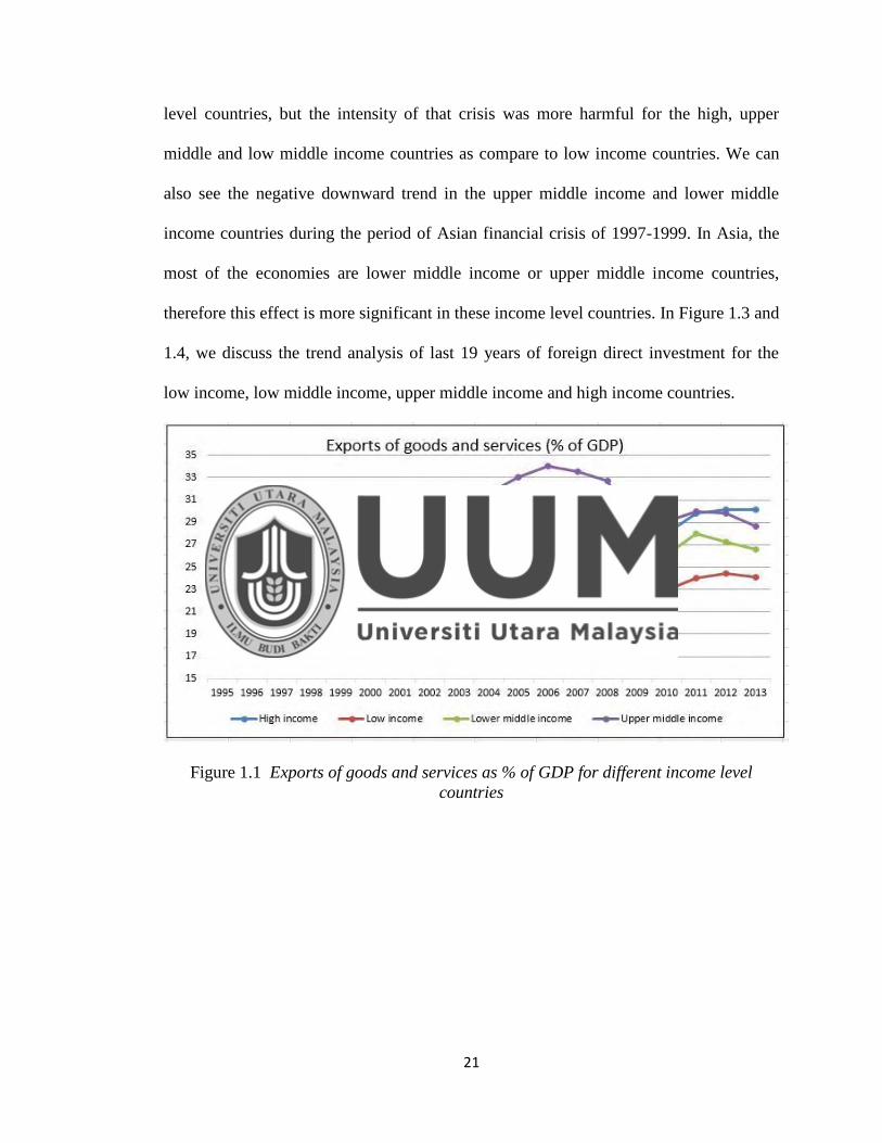
The trend analysis of exports available at Figure1.1 and 1.2 explain us that the upper
middle income countries are having the highest share of exports as percentage of GDP.
The high income countries are relatively low share as compare to upper middle income
countries, but it must be remain that in the high income countries the size of the gross
domestic product are much higher as compare to middle income countries. The low
income countries are having the lowest share of exports as %age of GDP as compare to
other income level countries. It can also be seen from the both Figures that the global
financial crisis of 2007-08 have significantly affected the share of exports in all income
21
level countries, but the intensity of that crisis was more harmful for the high, upper
middle and low middle income countries as compare to low income countries. We can
also see the negative downward trend in the upper middle income and lower middle
income countries during the period of Asian financial crisis of 1997-1999. In Asia, the
most of the economies are lower middle income or upper middle income countries,
therefore this effect is more significant in these income level countries. In Figure 1.3 and
1.4, we discuss the trend analysis of last 19 years of foreign direct investment for the
low income, low middle income, upper middle income and high income countries.
Figure 1.1 Exports of goods and services as % of GDP for different income level
countries

22
Figure 1.2 Exports of goods and services (Annual growth) for different income level
countries
Figure 1.3 Foreign direct investment as % of GDP for different income level countries
23
Figure 1.4 Foreign direct investment (Annual growth) for different income level
countries
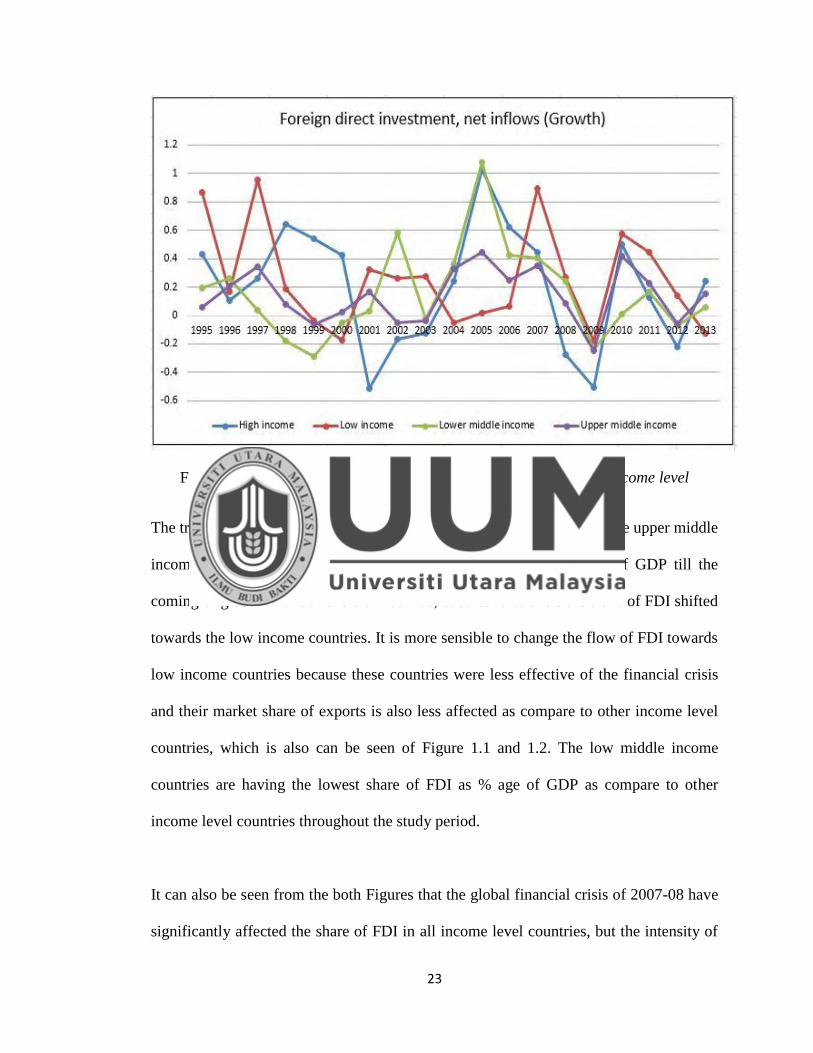
The trend analysis of FDI available at Figure1.3 and 1.4 explain us that the upper middle
income countries are having the highest share of FDI as percentage of GDP till the
coming of global financial crisis of 2007-08, but after that crisis the trend of FDI shifted
towards the low income countries. It is more sensible to change the flow of FDI towards
low income countries because these countries were less effective of the financial crisis
and their market share of exports is also less affected as compare to other income level
countries, which is also can be seen of Figure 1.1 and 1.2. The low middle income
countries are having the lowest share of FDI as % age of GDP as compare to other
income level countries throughout the study period.
It can also be seen from the both Figures that the global financial crisis of 2007-08 have
significantly affected the share of FDI in all income level countries, but the intensity of

24
that crisis was more harmful for the high, upper middle and low middle income
countries as compare to low income countries. We can also see that the Dot-Com bubble
crisis of early 2000‘s have also significantly affected the share of FDI in all income
level countries. The Asian financial crisis also affected in the negative downward trend
in the upper middle income, lower middle income and low income countries during the
period of Asian financial crisis of 1997-1999. However, the Asian financial crisis did
not severely affect the high income countries. In Figure 1.5 and 1.6, we discuss the trend
analysis of last 19 years of workers‘ remittances for the low income, low middle
income, upper middle income and high income countries.
Figure 1.5 Workers’ remittances as % of GDP for different income level countries

25
Figure 1.6 Workers’ remittances (Annual growth) for different income level countries
The trend analysis of remittances available at Figure 1.5 and 1.6 explain us that the
lower middle income countries are having the highest share of REM as percentage of
GDP till the 2013, but from 2013, the low income countries are almost having the same
share of REM as % of GDP as compare to lower middle income countries. We can see
that the share of REM has increased during the global financial crisis of 2007-08 in
lower middle income and low income countries. In the period of financial crisis, the
migrants send more money to their households for protecting their families from the
negative shocks of financial crisis. The same pattern we can also see in the period of
Asian financial crisis and Dot-Com bubble crisis. In Figure 1.7 we discuss the trend
analysis of last 19 years of external debt for the low income, low middle income, upper
middle income and high income countries.
26
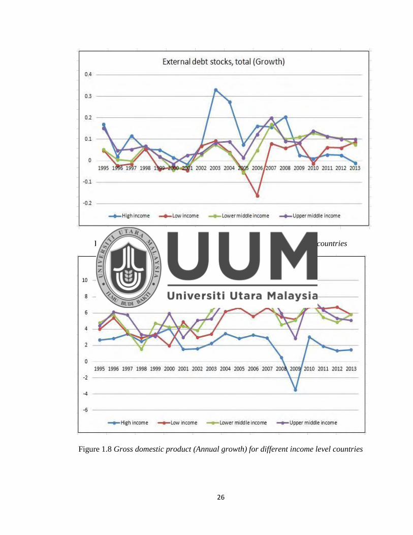
Figure 1.7 External Debt (Annual growth) for different income level countries
Figure 1.8 Gross domestic product (Annual growth) for different income level countries

27
The trend analysis of GDP available at Figure 1.8 show that the upper middle income
countries are having the highest growth rate in GDP in the last 19 years. The high
income developed economies are having the comparatively low but sustainable growth
in last two decades and till the occurrence of global financial crisis of 2007-2008. The
lower middle income and low income countries are having very mix and volatile growth
rates in the last 20 years. We can see that the GDP growth rate severely affected in the
period of global financial crisis. The high income countries are most effected in the
period of global financial crisis. The upper middle income is the second one whose
growth rate are down significantly. The growth rates in low income countries remained
comparatively stable in the period of global financial crises.
The same pattern we can also see in the period of Dot-Com bubble crisis. The growth
rates of upper middle, lower middle and low income countries were significantly down.
Whereas, the growth rate of high income countries was marginally effected. However,
in the period of Asian financial crisis the middle income and low income countries are
more effected as compare to high income countries.
1.3 Problem Statement
Foreign capital inflows play a significant role in the economic growth of developing and
developed countries (Raza & Jawaid, 2014). Foreign capital has been considered as a
key element in the process of economic globalization and integration of the world
economy. The flows of foreign capital have been welcomed, to complement domestic
financial resources, as a development catalyst. The experience of the newly

28
industrialized or emerging economies has firmed the belief that foreign capital could fill
the resource gap of the capital-deficient economies (Ali, 2014; Nkoro & KelvinUko,
2012).
These all foreign capital inflows play a vital role in the economic development of an
economy. Empirical studies conclude that these foreign inflows have positive as well as
negative impact on economic development and results vary between different countries.
Foreign direct investment (FDI) are perceived as a factor of economic growth, a
complement to domestic investment and a source of financing of the current account
deficit (Campos & Kinoshita, 2002; De Mello Jr, 1997). FDI contribute the host country
in the form of technological externalities, the formation of human capital or have access
to foreign markets which lead to long-term economic growth (Nicolini & Resmini,
2010). FDI also resulted a reduction in unemployment by creating more employment
opportunities in host economy (Siddique et al., 2012).
The entrance of FDI in the host country may also have negative influence on economic
growth. The introduction of new technologies assumes or requires the existence of
skilled labor in the host country, which are capable and trained of using those
technologies. If the supply of labor is short in host country than it leads to negative
impact on production and economic growth (Yousaf, Nasir, Naqvi, Haider, & Bhutta,
2011). Entrance of foreign companies in the imperfect competitive markets may leads to
reduce market share of domestic producers (Belloumi, 2014). Capabilities of economies
29
of scale also suffer in domestic producers because of loss of market share, which also
have a negative impact on productivity (Markusen & Venables, 1999).
Migrant workers‘ remittances are gradually becoming an important source of foreign
income for developing economies (Jawaid & Raza, 2014). More precisely, workers‘
remittances are found to be significant source of increase in investments and
consumption in host countries. Workers‘ remittances have been proved to be a source of
alleviating poverty in developing countries (Imai et al., 2011). The increase in workers‘
remittances also resulted in an increase in the private investments (Jongwanich, 2007).
Furthermore, remittances are found to be in a positive trend when the host economy
suffers a recession because of financial crisis, political conflicts or natural disasters etc.
as expatriates remit more during crucial time for so that they can support their families
and nations accordingly (Siddique et al., 2012).
Some empirical studies also found the negative impact of workers‘ remittances on
economic growth. The economic growth may have negative impact of capital inflows
(remittances) in the host country which causes the decrease in labor force participation.
This type of capital inflows may consider just as transfer of income. Furthermore, this
transfer of income may be stressed by severe moral hazard problem. In this regard, the
recipients promotes to use alternate way of consumption and the labor market effort
reduce accordingly (Jawaid & Raza, 2014). The migrant‘s remittances may not be
considered as profit driven due to spending on consumption rather than on investment
30
activities (S. Lim & Simmons, 2015). The imports may increase through remittances in
the country which further widen the deficit in balance of payment (Jouini, 2015).
In most of the developing countries, it is expected that when facing a scarcity of capital
would resort to borrowing from external sources so as to supplement domestic saving
(Sulaiman & Azeez, 2012). Soludo (2003) asserted that countries borrow for two broad
reasons; macroeconomic reason that is to finance higher level of consumption and
investment or to finance transitory balance of payment deficit and avoid budget
constraint so as to boost economic growth and reduce poverty. External debt is a major
source of public receipts and financing capital accumulation in any economy (Adepoju
et al., 2007). It is a medium used by countries to bridge their deficits and carry out
economic projects that are able to increase the standard of living of the citizenry and
promote sustainable growth and development.
Gohar et al. (2007) opined that accumulated debt service payments create a lot of
problems for countries especially the developing nations reason being that a debt is
actually serviced for more than the amount it was acquired and this slows down the
growth process in such nations. Daud, Ahmad, and Azman-Saini (2013) asserted that at
low levels debt has positive effects on growth but above particular points or thresholds
accumulated debt begins to have a negative impact on growth. Furthermore, Kasidi and
Said (2013) observed that high debt service payments shifts spending away from health,
educational and other social sectors.
31
The exports of a country play a vital and significant role to enhance the growth of the
economy (Omri et al., 2015; Tang et al., 2015). The spillover effect of the export sector
in the production process of an economy contributes in the total productivity of a
country. Moreover, export help in importing high value technology products and inputs
that cause increases in the productive capacity of a country which also leads to improve
the efficiency in the production process (P. Krugman, 1984; Lancaster, 1980;
Vamvoukas, 2007). The realization of economies of scale results export rise with the
help of rise in productivity. This increment in exports can further reduce cost, which
may also increase in the productivity growth (Helpman & Krugman, 1985). Moreover,
the possibility of negative linkage between economic growth and exchange rate may
exist, meaning that, rise in economic output level decline in the export growth level. On
the same note, the decrease in economic growth in the presence of export growth occurs
when growth in exports is appreciating against the domestic consumption (Dodaro,
1993).
In last two decades, the frequent occurrence of financial crises around the world, has
awakened the debate about the causes, consequences, impact and aftershocks of these
crises. In general, the financial crises are associated with problems in the banking sector,
the increased economic uncertainties, existence of "bubbles", globalization, climate of
financial instability or the periods when economies show poor performance. The
literature shows that foreign capital inflows are volatile and pro-cyclical and decline
during times of financial crisis. These patterns are more extreme in different income
level countries and have even motivated the use of the term ―sudden stops‖ to refer to

32
the large collapses in capital inflows that often accompany crises Cavallo & Frankel,
2008).
Previously, empirical studies report that the impact of financial crisis mainly decreases
the inflows of foreign capital in a country (Chor & Manova, 2012; Iacovone & Zavacka,
2009). These studies conclude that the economies which are heavily dependent on
external financing produce the worst performance in financial distress period. In the
period of financial crisis, the production and income of an economy is lower down. The
financial crisis leads to generate the negative sentiments among foreign investors about
future economic growth during the financial crisis period (Bogach & Noy, 2012;
Dornean et al., 2012; Skovgaard Poulsen & Hufbauer, 2011). Furthermore, the drop in
exchange rates during the financial crisis worse the economic conditions and it is
prolonged as long as government continues to monetize its deficit.
A currency crisis is considered a sudden loss in confidence and consequent depreciation
of the national currency in relation to other currencies, hence the importance of studies
on the speculative attacks, since in these cases is affected the real sphere of economy. In
recent years we have been witnessing the increasing occurrence of currency and
financial crises, both in developed or less developed countries. In last 20 years, the
world seen a 20 major events of financial crisis (banking crisis and currency crisis). The
countries have become more vulnerable and not able to predict financial and currency
collapses.

33
There are very few studies have been done which analyze the impact of financial crisis
on FCI and most of them are linked with the time series study of a specific country. The
movement of FCI is a matter of different income level countries and it is generally
moved from high and upper middle income countries to lower middle and low income
countries. The above discussion concludes that the foreign capital inflows (FCI) in the
form of foreign direct investment, external debt, exports of goods and services and
workers‘ remittances have significant influence over the economic growth, but the
results were contradictory and vary within the countries. Therefore, there is a need to
identify the relationship between FCI and economic growth on the homogenous panel
set of different income level countries i.e. low income, lower middle income, upper
middle income and high income countries.
Furthermore, it is also observing that the financial crises have a significant influence
over the flows of foreign capital in both developing and developed economies. These
financial crises effect the flow of foreign direct investment and international trade
among the countries. Furthermore, the required external debt for the development
projects are also become scare for the developing economies because of the consistent
events of financial crisis. The trend analysis discussed in the background section of this
study also highlighted the significant volatility in the flows of foreign capital during the
period of financial crisis (banking crisis and currency crisis). Therefore, there is a need
to identify the relationship between FCI and economic growth in the presence of
currency crisis and banking crisis on the homogenous panel set of different income level
countries.
34
1.4 Research Questions
Several questions arise from the problem statement, which include:
1. What is the impact of foreign direct investment, foreign debt, workers‘ remittances
and exports of goods and services on economic growth in high, upper middle, lower
middle and low income countries?
2. What is the impact of foreign direct investment, foreign debt, workers‘ remittances
and exports of goods and services on economic growth in high, upper middle, lower
middle and low income countries in the presence of currency crises.?
3. What is the impact of foreign direct investment, foreign debt, workers‘ remittances
and exports of goods and services on economic growth in high, upper middle, lower
middle and low income countries in the presence of banking crises?
1.5 Objective(s) of the Study
The general objective of this study is to identify the impact of foreign capital
inflows on economic growth of different income level countries in the presence
of currency and banking crises. Specifically, this study aims at the following
objectives:
1. To examine the impact of foreign direct investment, foreign debt, workers‘
remittances and exports of goods and services on economic growth in high, upper
middle, lower middle and low income countries.
2. To examine the impact of foreign direct investment, foreign debt, workers‘
remittances and exports of goods and services on economic growth in high, upper
middle, lower middle and low income countries in the presence of currency crises.
35
3. To examine the impact of foreign direct investment, foreign debt, workers‘
remittances and exports of goods and services on economic growth in high, upper
middle, lower middle and low income countries in the presence of banking crises.
1.6 Justification and Contribution of the Study
Theoretically and empirically it seems that foreign capital inflows have different
possible effects on growth and development performance of an economy. If foreign
capital inflows are used in an efficient and productive manner then, they will promote
country‘s growth performance. If foreign capital inflows are used in unproductive
manner then they will not contribute in a long run, their impact on economic
development will only for a short run. Furthermore, the financial crisis (currency and
banking crisis) also have a significant influence in the attraction of foreign capital
inflows. These financial crises effect the flow of foreign capital inflows among the
countries. Furthermore, the required external debt for the development projects are also
become scare for the developing economies because of the consistent events of financial
crisis. In last 20 years, the world seen a 20 major events of financial crisis (banking
crisis and currency crisis). The countries have become more vulnerable and not able to
predict financial and currency collapses.
There are very few studies have been done which analyze the impact of financial crisis
on FCI and most of them are linked with the time series study of a specific country.
Empirical studies show that the behavior and relationship of foreign capital inflows with
economic growth has varies from country to country. The movement of FCI is a matter

36
of different income level countries and it is generally moved from high and upper
middle income countries to lower middle and low income countries. Therefore, we need
to analyze the relationship of foreign capital inflows with economic development in the
presence of currency crisis and banking crisis, in high income, middle income, and low
income countries separately to better judge the behavior of foreign capital inflows.
This study fulfills the missing area of research in foreign capital inflows (FCI) by
evaluating the relationship between foreign capital inflows and economic growth of
countries with different income levels. The major contribution of this study is to analyze
the influencing role of currency crisis and banking crisis on the relationship of foreign
capital inflows and economic growth. In this research, we divided the financial crisis in
two broader forms of crisis i.e. banking crisis and currency crisis. Furthermore, the
major methodological contribution of this study is lies in the measurement of currency
and banking crisis for each country. In past studies, the researchers just use the dummy
variable of financial year in which the main crisis event occurred in the World to
analyze the influence of financial crises on considered variables. For Instance, for the
period of Global financial crisis they put the value 1 for 2007-2009 and for the other
years they put zero. However, it is empirically proved that the Global financial crisis did
not mainly affect many Asian countries. Therefore, it is not appropriate to consider the
year of financial crisis for the whole world.
Therefore, to cover this issue we have measured the period of currency and banking
crisis specifically for each country by using a unique methodology which is discussed in

37
details in the chapter of Methodology. Another major contribution of this research is to
use the different items of foreign capital inflows of any country. In most of the past
studies researchers used only one item to analyze the impact of foreign capital inflow on
economic development of economies. But in literature there are more than one indicator
are available to analyze the overall foreign capital inflows of any country.
This study is using four major items of foreign capital inflows, which play a major role
in the economic development namely; foreign direct investment, workers‘ remittances,
external public debt and exports of goods and services. These four items are the main
sources of foreign capital inflows for the countries. This study analyzes the relationship
of four major items of foreign capital inflows with economic growth in high income,
upper middle income, lower middle income and low income countries to better judge the
relationship between foreign capital inflows and economic growth. This study will be
beneficial for all economies either the high income, middle income or low income.
This study also provides policy recommendations to policy makers of all targeted
countries. This study provide the comparison of investment in different income level
countries for the foreign investors. The study will also provide guidance to foreign
investors in taking the investment decisions in different income level countries in the
period of financial crises. Furthermore, the results of this study will also help the policy
makers to formulate the policies related to foreign capital inflows in the period of
financial crises. This study will also provide useful information about the role of

38
external debt in the process of economic growth in different income level groups. The
results of this study will help the policymakers to formulate better debt policies.
1.7 Scope of the Study
This study examines the impact of foreign capital inflows on economic growth of
different income level countries. Furthermore, this study also analyzes the relationship
of foreign capital inflows and economic growth in the presence of currency and banking
crises. We collect the balanced panel data of 96 countries and group them on the basis of
different income levels. The final sample of this study consists of 10 low income
countries, 23 lower middle income countries, 30 upper middle income countries and 33
high income countries. This study covers the period from 1995 to 2013.
This study is using four major items of foreign capital inflows, which play a major role
in the economic development namely; foreign direct investment, workers‘ remittances,
external public debt and exports of goods and services. These four items are the main
sources of foreign capital inflows for the countries. This study analyzes the relationship
of four major items of foreign capital inflows with economic growth in high income,
upper middle income, lower middle income and low income countries to better judge the
relationship between foreign capital inflows and economic growth.
We also use the set of control variables based on the potential and significant
determinants of economic growth to control their effects in our model. These important
determinates of economic growth as a control variable are adopted from the seminal

39
work of Levine and Renelt (1992) and Barro (1996). These control variables are also
endorsed by various researchers as important determinants of economic growth and still
in the recent studies these variables are using as main determinates of economic growth
such as; (Delgado, Henderson, & Parmeter, 2014; Eggoh & Khan, 2014; Glewwe,
Maïga, & Zheng, 2014; Law & Singh, 2014; Manamperi, 2014; Martins & Veiga, 2014;
Menyah, Nazlioglu, & Wolde-Rufael, 2014; Teles & Mussolini, 2014)
1.8 Plan of the Study
The thesis is arranged as follows: chapter one consists of the introduction of foreign
capital inflows and economic growth, statement of the problem, objective of the study,
justification of the study and scope of the study, Chapter two is the theoretical and
empirical literature on the relationship of foreign capital inflows, banking crisis,
currency crisis and economic growth. Chapter three comprises of the methodology,
model specification, sources of data and description of variables. Chapter four is for
presentation of results and discussion. Chapter five contains summary of major findings,
conclusion, recommendations, limitation of the study and recommendation for future
research.
1.9 Summary of the Chapter
Foreign capital has been considered as a key element in the process of economic
globalization and integration of the world economy. The flows of foreign capital have
been welcomed, to complement domestic financial resources, as a development catalyst.
Foreign capital inflows are perceived as a factor of economic growth, a complement to

40
domestic investment and a source of financing of the current account deficit (DeMello,
1997; Campos and Kinoshita, 2002). Foreign capital inflows contribute the host country
in the form of technological externalities, the formation of human capital or have access
to foreign markets which lead to long-term economic growth (Nicolini and Resmini,
2010). Foreign capital inflows also resulted a reduction in unemployment by creating
more employment opportunities in host economy (Siddique et al., 2012).
In last two decades, the frequent occurrence of financial crises around the world, has
awakened the debate about the causes, consequences, impact and aftershocks of these
crises. International economic integration puts a country‘s fortunes partly into the hands
of others. Previously, empirical studies report that the impact of financial crisis mainly
decreases the inflows of foreign capital in a country (Ronchi, 2004; Iacovone and
Zavacka, 2009; Chor and Manova, 2010). These studies conclude that the economies
which are heavily dependent on external financing produce the worst performance in
financial distress period.
There are very few studies have been done which analyze the impact of financial crisis
on FCI and most of them are linked with the time series study of a specific country. The
movement of FCI is a matter of different income level countries and it is generally
moved from high and upper middle income countries to lower middle and low income
countries. This study analyze the relationship between FCI and economic growth in the
presence of currency crisis and banking crisis on the homogenous panel set of different
income level countries.

41
CHAPTER TWO
LITERATURE REVIEW
2.1 Introduction
In this chapter, we review both theoretical and empirical literature on the relationship of
different types of foreign capital inflows and economic growth. The starting point of
every empirical research on economic growth has been with the discussion of the neo-
classical theory, Solow growth model, endogenous growth theory and exogenous growth
theory. Theoretically, the foreign capital inflows contribute into the process of economic
growth by both endogenous and exogenous factors. The theories are discussed below,
and then followed by review of empirical studies on different types of foreign capital
inflows and economic growth.
2.2 Theoretical background
In this section, we discuss the different theories related to economic growth, foreign
direct investment, exports of goods and services, workers‘ remittances and external debt.
Furthermore, we also discuss the theoretical channels through which different types of
foreign capital inflows affect the economic growth.
2.2.1 Theories of Economic Growth
The theory of growth can thus be defined as the branch of economics that studies the
historical growth of gross domestic product (GDP) of the various countries or regions,
an almost exclusively by the GDP growth and GDP per capita, because it assumes that
42
the well-being of the populations is strictly correlated with these indicators (Sen, 1997).
In this sense, economic growth refers to growth that is home to the expansion of GDP in
a particular country. When we assess the commitment or the efficiency of a given
economy, resorted to GDP per capita, since this indicator gives us absolute data, i.e.
GDP Figures depending on the population of a country. This indicator is important since
one particular country can present a high GDP depending on the size of its population,
but this value can be assumed as insignificant when compared with the other countries
that have a relatively low GDP.
In fact, this finding highlights the importance of considering the development indicators
in a comprehensive sense, since by itself, may not take into account any existing
inequality in the distribution of social income, such as mark. Even though currently the
GDP per capita is not an indicator par excellence which measures the well-being of the
population, it cannot be negligible in assessing the efficiency of an economy, since the
component where it derives is assumed as an engine for growth (Young, 1994).
There are basically four parts or wheels that are assumed, by most economists, as the
engines of growth of a country, and can these elements be distinctly exploited to reach
the result, taking into account the different features that are part of each country. From
among these, we highlight the capital accumulation, technological progress, human
resources and natural resources (C. I. Jones & Romer, 2009).

43
The capital of a country can be analyzed from the existing viable infrastructure,
machinery, trucks, intangibles, among others. When a given country accumulates
capital, this means that increases its production capacity. This mechanism of
accumulation is favored when there is an available savings that companies use to invest
through financial intermediaries. When there is investment, there is an accumulation of
physical capital and, in this perspective, there is a strengthening of the means of
production and the consequent increase in production, due to the existence of good
communication infrastructure, power plants and good lines of communication that help
corporate productivity (Belloumi, 2014).
The second aspect refers us to the state of the art technologies, which is a great indicator
of the transformation processes that influence economic dynamics. Technological
progress includes different types of innovations, in particular, incremental innovations,
which improve the production processes from what already exists, but also radical
innovations that create new production processes and new products (Sharma & Abekah,
2008).
The growth has created new limits and has been driven social and technological changes
that affect productivity at work in organizations. Technological progress assures that
there might be a higher output with the same amount of work equipment (Sen, 1997). In
this line of thinking, population growth, increased employment and innovation, assume
as decisive factors in the cycle of economic growth. These factors interact in particular
in various contexts, characterized by historical routes and private institutions. It is clear

44
that, over time, increased knowledge and the availability of more sophisticated
techniques become workers and equipment more productive (Sharma & Gani, 2004).
Human capital is assumed to be one of the most prevalent factors in the development of
a country, because a nation can have many natural resources, cutting-edge technology, a
substantial physical capital, but if you do not have qualified human resources, will
quickly be confronted with difficulty in integrating these other resource with human
resources in the labour market. This aspect assumes particular relevance in many
countries, such as the Netherlands, where for example, although there are no large
natural resources, there is a great investment in terms of human resources, putting this
country into a higher ranking relative to other countries in possession of natural
resources and advanced technology (Sen, 1997; Sharma & Abekah, 2008; Sharma &
Gani, 2004).
When human resources are well trained and qualified, they become a capital, i.e. an
asset since contribute efficiently and effectively for the production, and their
productivity is enhanced, providing positive benefits for the company, whether in the
national context is in the international context. Internationally, this differentiation of
human capital assumes fundamental importance, as this may constitute an attractive
factor for FDI, especially in sectors of activity in which it is essential to the FDI
component. Therefore, nowadays, the focus on training and technical qualification of
human resources is regarded as a great investment for the growth of a nation (Sen, 1997;
Sharma & Abekah, 2008; Sharma & Gani, 2004).
45
Another very important factor which attracts contribute in the economic growth of an
economy is the availability of natural resources; i.e. productive and agriculture land, oil,
gas, forests, water and mineral resources. Some developed countries, such as Canada
and Norway, have grown thanks to the breadth of its primary natural resources, with
large oil and gas production, agriculture, fisheries and forest resources. Similarly, the
United States of America (USA), with its fertile agricultural land, is the largest producer
and exporter of cereals.
However, the existence of natural resources is not a necessary condition for economic
success in the modern world. Such as the New York City, for example, thrives primarily
due to its dense network of industries and service businesses. Many countries such as
Japan, have virtually no natural resources, but it evolved through specialization in
certain sectors that rely heavily on more work and human capital than natural resources.
In fact, as Young (1994) advocates, possessing only a tiny portion of the area of Nigeria,
which is rich in natural resources, the tiny city of Hong Kong has, effectively, a GDP
greater than that great African country.
In this sense, the natural resources seem to be sufficient, but not necessary condition for
the development of a nation, because there are countries with huge potential, as is the
case of the Democratic Republic of the Congo, and that lie within the last rating of HDI.
For this reason, it is important to analyze the rationality of the management of the
country which has many natural resources and who can optimize, providing a greater
advantage for their development, since it attracts investment, minimizing the cost of

46
transactions, given the existence of other significant infrastructure, such as the distance
between the company and the source of supply of raw materials (Baldwin, 2004).
The theories of growth turned in General to understanding the phenomenon of growth,
abstracting in general trade relations between countries. Only more recently has been
developed effort to integrate trade to economic growth models. The theories of growth
can be classified in two generations: (a) neoclassical theories; and (b) new theories of
growth, including endogenous growth.
The neoclassical models were developed first by Solow (1956) and Swan (1956)
prevailed as a reference for the analysis of growth for several decades. The assumptions
about the markets and the production are essentially identical to those of the neoclassical
theories of trade. The markets are perfectly competitive, and the production function of
the genus Cobb-Douglas. Typically, are employed in two production factors: capital and
labor force. The work expands on the basis of demographic dynamics, external to the
model. The capital is accumulated in function of external forces, especially those that
determine the technological progress. The accumulation of capital, however, suffers
from a limitation, that comes from the production function approach of production.
According to this approach, the marginal productivity of capital is, by definition,
descending. Thus, the rate of capital accumulation and, ultimately, the growth of the
economy converge to a potential balance given exclusively by their fundamental
characteristics. In other words, there is exogenous growth, without which certain
policies, notably the commercial, to be able to change the potential rates of growth.
47
Under these conditions, the trade does not tend to affect the rate of growth of
economies. This is determined in long-term balance by exogenous factors, such as the
rate of expansion of the productivity and the structural characteristics of the economy.
Relations between trade and growth does not modify the rate of growth of the economy,
and this the same in local environments or free trade.
Such restrictions were not necessarily implied in some traditional models of growth, like
those of Harrod and Domar3, formulated even before those of Solow and Swan. Unlike
the neoclassical tradition, growth models of the genre of the seminal Harrod and Domar
didn't uphold in production function. Assume that the marginal return of capital may be
constant and positive, not limited because of that factor accumulation and economic
growth to a single trajectory.
In contrast to the neoclassical models, such seminal Zhukov demonstrated growth
models right space for public policy intervention, the effects of which could alter the
rates of savings and investments and thus raise or reduce the growth rates of the
countries. According to Thirukodikaval Nilakanta Srinivasan and Bhagwati (1999),
"even the steady state growth rate is sensitive to policy". This fee would not be
determined by exogenous mode and could be intensified by generating "growth effects
from trade policy". Different trade policies and, in particular, trade liberalization could
therefore cause "dynamic" gains, raising the rates of economic growth in the long term
(Thirukodikaval N Srinivasan, 1995). However, the success of the policies and their
corresponding gains in growth would depend on favorable environment, which was not
3 For details see, Harrod (1939) and Domar (1946)
48
distorted by market failures. Thirukodikaval Nilakanta Srinivasan and Bhagwati (1999)
argue that such failures can easily compromise the gains of trade policies.
The new growth theories relating the dynamics of endogenous growth of economies.
Developed originally by Paul M Romer (1986) and Robert E Lucas (1988), these
enhance the mechanisms anticipated by the seminal models and are capable of
engendering sustained capital accumulation. Within the framework of these theories are
determining the accumulation of human capital, innovation and technological
diversification. In these cases, externalities are emerging as technology and human
capital, as different forms of knowledge can be disseminated among agents, both within
the firm, aggregated terms in the industry. The growth may converge and sustain the
higher rates, provided they are the higher the rates of accumulation of knowledge
applicable to production. The accumulation of knowledge is through education,
learning, training of manpower and various activities of research and development
(R&D) and technological innovation. Growth perpetuates endogenous manner insofar as
the marginal product of capital, physical or human, remains positive, stimulating
accumulation of knowledge activities, in different ways. Some models, based on these
conditions, tend to show that FCI allow you to increase productivity and economic
gains, through exports, foreign direct investment external debt and workers‘ remittances.
Increased competitiveness through imports and exports, and the benefit of the use of
scales, to meet external demands, can induce processes of accumulation of knowledge.
Grossman and Helpman (1991) argue that the human capital directly associated to R&D
and can contribute to the creation of new intermediate goods and boost growth and

49
trade. However, as Baldwin (2004), in models such as Grossman and Helpman, "there
is no definite answer to whether protection increases or decreases the growth rate. It
depends on the pattern of imports and exports". Trade policy and others may discourage
the production dynamic sectors, exporting, and potentially hinder the diffusion of
productivity gains, including from the imports of intermediate and capital goods. To a
large extent, the reaction of economies to liberalization depends on the structure of the
economy, the economic pattern of its international insertion and executing policies in
various fields, ranging from educational, scientific-technological and industrial to
financial and macroeconomic.
Unlike traditional theories, the endogenous growth theories allow you to conclude that
the foreign capital inflows and growth models nourish a dynamic of mutual causation,
and the gains are no longer static. This dynamic is based on dynamic character of
production, its diversity and dependence in innovative processes or human capital
intensive, State intervention and public policies in favor of those processes can increase
the dynamic gains from foreign capital inflows and growth and strengthen each other.
However, as concluded by Lawrence and Weinstein (1999) that this theory is actually
ambiguous on the dynamic effects of foreign capital inflows trade. In some situations,
could even the dynamics become counterproductive, generating lower growth and well-
being. Therefore, according to argue Long and Wong (1997) vis-à-vis possible
ambiguity and diversity of theoretical results, "on simple policy recommendations
50
should be made without a thorough understanding of the structure and the key features
of the economies under consideration".
There are vast literature discuss the theoretical linkages between the foreign capital
inflows and endogenous growth. The challenge of these models is to reconcile the
processes of technological development and accumulation of capital (mainly human),
own growth, with the processes of allocative and productive efficiency, as well as
technological diffusion, which can be stimulated by international trade. C. I. Jones and
Romer (2009), argue that the integration of foreign capital allow you to enlarge the scale
of markets, production and, especially, the dissemination and absorption of knowledge
and ideas. Thus, growth-oriented economies increasingly greater benefit would be the
endogenous of globalization. The literature shows there are serious chances that
externalities and trade growth to build up in countries that invest in the processes of
induction of endogenous growth.
These investments, coupled with appropriate policies, they multiply the gains of foreign
capital inflows. Lucas Jr (1993) indicates that, in some circumstances, the protection can
allow the maturation of long-term comparative advantages, especially in high-tech
sectors. Young (1994) shows how the protection of less developed countries and as
subsidies to sectors of highest technology can also bring greater benefits. In these cases,
the benefits of liberalization are earned only if it is subject to a prior sequencing of
policies in support of infant industries. Similar argument would apply to intellectual
property rights and the protection of these rights allow easing to technologically less

51
developed economies to mature their inventive capacity. Initially could prevail breeding
technological activities, lower costs, but if the relaxation of protection is accompanied
by set of policies, including increasing openness, economic environment could be
stimulated more intensively innovation and technological diversification.
In fact, the foreign capital inflows can be income differences and inducer of growth
among countries, depending on the position or relative slope of the countries. As the
processes of accumulation is based on aggregation of intangible value, the basic policies
(industrial, educational, scientific-technological) to induce these processes can weigh as
much as or more than the allocations of resources and structural characteristics.
2.2.2 Foreign Direct Investment and Economic Growth
The existing literature on the relationship of foreign direct investment (FDI) and
economic growth does not have unanimous results. Some of these studies point to the
fact that the FDI generate economic growth from technological progress and the
accumulation of capital, which increases the productivity of companies and,
consequently, growth. However, other studies conclude that the FDI is not always
assumed as a vector for growth. Indeed, the FDI can create barriers and lead to an
inability to adapt national companies, having a damaging impact on the whole economy
(with perverse effects on the level of unemployment, increase in the number of bankrupt
companies and the loss of national sovereignty due to mostly presence of foreign firms
instead of local firms).

52
Specifically, in developing countries, there are still many difficulties which affect the
well-being of populations, due to the scarcity of financial resources, and the FDI is
identified as a shape that can promote the resolution of structural problems found in
some of these countries. The relevance of this scientific study seems clear, especially
since the studies on this theme applied to the different income level countries are
missing in the literature. Its usefulness extends eventually political decision-makers
wishing to implement policies that promote economic growth.
The concept of FDI is associated with those foreign companies or foreign investors (in
this case sender), which promote the creation or taking possession of a firm in another
foreign location (in this case receiver), in order to perform their activities profitably,
with a view to their control over the function of firm. The emerging or developing
countries seek to attract FDI, since it assumes as an important source in the fundraising
needed to solve structural problems and related to the well-being of the population, since
in these countries, these financial resources are scarce. In this line of thought, the FDI is
considered by several international, political and economic institutions as a generator of
economic growth and a solution to the economic problems that is facing by developing
countries (Mencinger, 2003).
In this sense, we can say that the FDI is a component that generates growth when
countries use it rationally, that is, the result of their activities should be satisfactory for
both transmitters and receivers. The issuing country must carry out a study in advance
regarding the opportunities and threats in the country, decision of investment should be

53
based on the feasibility of the business, as well as the strategies that should be
implemented in order to minimize the risk inherent in investing. This idea actually meets
the economic theories that suggest that foreign capital flows, when allocated efficiently,
they generate economic growth (Mencinger, 2003).
As Carkovic & Levine, (2002) argue that these multinational companies are thus an
essential source of financial, technological and organizational resources for least
developed countries. This type of investment includes the control of a company, or part
of it, in a foreign country, being accompanied by creating employment opportunities,
transfers of technical resources, knowledge, human capital development and many
others ways. The key to distinguish the FDI in other ways of operation is that the
company has a control over the assets of which are holding abroad.
If we take this aspect into account, easily understand that countries with weaker
economies take the FDI as the source of growth and modernization of the economy
(Carkovic & Levine, 2002; Ford, Rork, & Elmslie, 2008). Therefore, the receiver
countries should ensure the business-friendly environment for the inflows of FDI in
micro and macro perspectives, especially ensuring political stability to attract investors
and to benefit from the advantages that these investments contribute to your country, in
economic, social and political terms (Carkovic & Levine, 2002).
The estimates resulting from the Economist Intelligence Unit [EIU] (2014) point to the
fact that the FDI have been increasing in recent decades and underline its growth in the

54
future. Thus, about 15% of FDIs are now focused on developing countries, which may
be justified, in part, by the relocation of industrial activities and production of labour-
intensive, particularly to China, since here are rates of return on investments usually
higher than in developed countries.
In last three decades, the impact of FDI on economic growth is widely studied (Carkovic
& Levine, 2002; M. E.-G. Lim, 2001; Sylwester, 2005), doubts still persist with regard
to their effects, as well as what are the necessary conditions and resources that provide
economic growth (Venkataraman N Balasubramanyam et al., 1996). In fact, even
though several studies point to the positive effects of FDI, some authors underline the
discrepancy of positions in relation to the degree of effects caused by the FDI in the
country (Blomström & Kokko, 1998; M. E.-G. Lim, 2001). In a short, we can say that
the FDI is a major source to formulate the gross capital formation, which can generate
the growth of the developing countries.
In this section, we present some of the theories that have emerged in the explanation of
the FDI, including the theory of monopolistic advantage, an oligopolistic behavior
theory, theory of internalization, transaction costs theory, theory of location advantages
and theory of product life cycle.
First of all we discuss the theory of monopolistic advantage, this theory focuses on the
monopolistic advantages of Multi-National Corporations (MNCs). According to
Kindleberger (1969) and R. B. Cohen and Hymer (1979), the existence of the MNCs
55
stems from the fact that these have some kind of knowledge or competitive advantage,
of monopolistic nature, which allows them to compete with local companies, describing
the specific advantages of the company as a manifestation of structural imperfections of
the market and consequent existence of oligopolistic benefits.
Kindleberger (1969) stated that it constituted a necessary condition to the FDI, the
market of goods and services were flawed or that there was an interference in
competition on the part of the Government, given that local businesses would have
advantages over the multinationals due to the proximity of the decision-making centers.
Therefore, the structure of certain markets would determine the appearance of the FDI.
From the perspective of R. B. Cohen and Hymer (1979), a company it is necessary to
have some kind of financial advantage, technology, management, marketing or
production to reduce or minimize the chances of failures in the new consumer markets.
In short, this theory argues that is the existence of market imperfections of products,
economies of scale and to government intervention in markets, which feed the FDI.
However, the weakness of not consider the factors that affect the choice of the location,
nor the reason why companies choose the FDI as a mechanism of operation abroad and
explore the so-called advantages of properties.
The theory of oligopolistic reaction is based on the assumption that the internalization of
a company engaged in an oligopolistic market (being that she herself is oligopolistic
also) results from the reaction to the internalization of a competing company.
Knickerbocker (1973) the founder of this theory argue that when a foreign company
56
performs an FDI, other companies often exhibit imitative behavior, i.e. they follow the
internationalization of competitors so that they will not lose their strategic advantage.
It is argue that oligopolistic firms seek stability, which is to maintain and consolidate a
position in the oligopolistic market, both locally and internationally. Therefore, one of
the determinants of FDI is the motivation of certain foreign companies follow the
example of competing companies. Thus, the one major strategy of investing abroad is to
generates a chain reaction among its competitors, since it seeks to maintain the balance
and the same conditions between all participants of the oligopoly irrespective of market
location, running the risk of not obtaining attractive rates of return and even get negative
rates of return at least for a certain period of time.
It emphasizes that the MNCs produce more benefits resulting from diversification of
investments that perform, thus reducing the risks of a downturn and negative
environments on the market. Previous theories do not explain the reason why companies
choose to explore their monopolistic advantage through the FDI and thus arises the
theory of internalization that is based on the existence of gaps in goods markets and
factors that may induce businesses to FDI.
Thus, among the projects developed around this theory include those of Buckley and
Casson (1976) that underline the necessity of existence of four groups of factors so that
this theory can be put into practice: (a) industry-specific factors, related to the nature of
the product and with the structure of the external market; (b) specific factors in the
57
region, arising from his social and geographical features; (c) country specific factors
associated with their political and fiscal relations and; (d) company-specific factors,
which reflect the ability of management structures in organize an internal market. In this
sense, the intermediate product market integration through the FDI, would enable the
reduction of costs.
Therefore, the company develops a specific advantage in their home market, possibly in
the form of some intangible assets (e.g., marketing or production management), which
gives some advantage compared to other companies, including local companies. In
short, the internalization of transactions, from the FDI, you can take on the best way to
explore the intangible assets (e.g., knowledge) and transcend their own market
imperfections. With the internalization can be avoided the imperfections and companies
can expand their activities to other markets, thus reinforcing its advantages.
This transaction cost theory was presented by Coase (1937) and it states that transaction
costs refers to the cost of providing for some good or service through the market rather
than having it provided from within the market. This theory assumes an intention to
justify the reason for a company to opt for FDI engine, instead of export or enter into
contractual relations with the outside world, stating that this aspect results from the use
of its advantages of ownership.
In fact, in the case where the cost of the transaction through an organization is smaller
than the exchange through the marketplace, the company grows by internalizing the

58
market to the point of getting the benefits that its action to offset their costs, plus a better
use of economies of scale and scope that reduce the cost associated with the transaction
information, opportunism and uncertainty. In short, according to this theory, the unit of
analysis was the transaction and the goal would be to minimize the transaction costs
associated with each alternative that could be presented.
Under this theory of location advantage, the foreign company operates its activities
where there are lower costs. In fact, the location factors are capable of motivating for the
internationalization of the company in search of natural, technological or financial
resources abroad, in order to better your value chain (Durán & Ubeda, 2001). Therefore,
the location factors are conditioned by characteristics of the country of destination of
FDI, by its prevalent economic system, for its cultural, social, political environment by
the availability of resources in the country and by their own characteristics in the
internal market.
For Instance, it is arguing that oil companies invest where there are oil reserves and, for
their exploitation, combine their technical and management capacities with the local
resources available (e.g., workforce, knowledge or progress in semiconductors and
computers). However, from the perspective of these authors, the selection of location is
not always as obvious, since there are a multitude of factors that influence the choices,
namely:
a) Some activities can generate increasing economies of scale, reducing
substantially the cost through increased utility of quality produced. In this case,
59
there is an incentive to increase the scale of current operations and the
achievement of an investment in new subsidiaries abroad.
b) The production is not a single phase in the value chain, from what companies
need to analyze their activities at the perspective of research and development
(R&D) or marketing, looking for locations that minimize their costs. For
example, we can say that the R&D might be better located in regions where there
is more material used or skilled workers to do so. With regard to marketing, this
integrates aspects such as the state of development and operation of distribution
channels, limits and restrictions on advertising campaigns, price fixing, among
others, which requires, necessarily, markets with particular and specific
characteristics.
c) Some companies can influence the prices of production factors in a given region,
so will tend to locate their intensive production processes of these factors (or
factor) at that location.
d) It is still necessary to consider the impact of government intervention (e.g.,
through fares, taxes, fees, preferential duty), which influences the advantages of
each location. The Governments of certain countries such as China, using trade
barriers to encourage FDI to the detriment of exports.
e) Finally, the work is not the only factor that must be taken into account. Although
labor costs may be relatively low in certain countries, it is necessary to consider
other aspects, such as the qualification and training of manpower available, since
the lack of specific training will entail a cost in their training.

60
The theory of product life cycle suggests that some types of product undergo a cycle,
composed essentially by four phases: (a) introduction; (b) growth; (c) maturity and; (d)
decline. Therefore, in the first phase of introduction, firms can register small-scale
exports to other countries; in the second stage of growth, firms can produce a total or
partial relocation of production to foreign countries, where the cost of transport or
customs barriers are sufficient to justify the decentralization of production; in the third
stage, a particular aspect is the transfer of production to developing countries, in order to
obtain certain advantages in costs and, in the last phase, demand grows in these
developing countries, which is where he produces, mostly the product and from where
exporting to developed countries.
This theory of product life cycle argue that when a foreign market is large enough to
support local production, the foreign company performs investment, i.e. FDI.
Summarily and given the perspective of Vernon (1966), we can say that the theory of
product life cycle has present the advantages of the location of countries and its
relationship between the production of certain types of goods, in each one of the stages
of their life cycle, and the innovation of products would be an eminent condition,
especially in countries with large capital and economic development.
2.2.3 Foreign Debt and Economic Growth
The debt of a country can be measured and analyzed in different ways. First it is
important to define and separate the various types of debt that can be associated with a
country. Debts relating to a country can be public or private. Public debts are, naturally,

61
those that are contracted by the State. On the other hand, private debts are those that are
incurred by private entities (be they individual or collective entities).
The debt contracted by the State is usually referred to as public debt; they can be divided
into internal public debt and external debt (also called for sovereign debt). The public
debt is defined as the aggregate of all debts incurred by various organs of the State. The
origin of the public debt is associated mainly to three factors: public spending on goods
and services, spending on interest on debts previously and still derived from foreign
exchange and monetary policies. In turn, the public debt can then be debt between
domestic debt and foreign debt. The debt with respect to the internal part of the public
debt which is composed of the debts contracted by the Government with national
lenders. Such debts are usually contracted with the internal market, in particular by way
of the issuance of debt securities. On the other hand, the external debt is the sum of the
debts contracted by the Government with foreign creditors, be from other States, foreign
banks, IMF, or any other type of entity.
However, there are several ways to "measure" the external debt of a country. Andini and
Cabral (2012) argue that the external debt stands out mainly in terms of gross external
debt, the international investment position and external debt. Gross foreign debt is the
sum of total debt instruments from residents to non-residents, namely corresponds to the
total foreign debt which is formed by public and private foreign debt. The international
investment position corresponds to the difference between financial assets and liabilities
of residents vis-à-vis non-residents. And, finally, the net external debt is equal to the
62
gross foreign debt minus the sum of total debt instruments of non-residents to residents.
Reinhart and Rogoff (2009), define debt as being the total liabilities of a country (public
and private) with foreign creditors, namely corresponds to gross external debt. On issues
relating to debt crises the generality of literature turns out to follow this external debt
definition. In this way, in accordance with most of the existing literature, this will also
be the definition of external debt followed throughout this dissertation.
Among the existing literature a foreign debt crisis of a country corresponds to the non-
compliance, or risk of non-compliance with the obligations of a country from its foreign
creditors. Noting that a debt crisis can take two forms: (i) when the Government of the
country needs to restructure its debt, or (ii) when the country's Government goes into
default-total failure of its obligations. A debt restructuring is nothing more than a
renegotiation of loan terms. Today many of these restructurings are performed with the
aid of the International Monetary Fund (as an example we have the current case of
Greece). Reinhart and Rogoff (2008) claim that these constitute a partial default. First,
because debt restructuring often involve reductions in interest rates.
Secondly, and probably more important, is the fact that debt restructuring normally
arrest investors with illiquid which are not renumbered for decades. This illiquidity is a
huge cost for investors, forcing them to hold assets with risk, they often have
compensations on much below market. On the other hand, the entry of the Government
of a country in default is the extreme case of a debt crisis, translating a complete
inability on the part of the country to comply with its obligations with creditors. It's

63
about this situation that the majority of existing literature focuses your attention. In
addition to these two types of situation, amid the economic literature there are some
studies that assume the existence of a crisis when a country uses a large amounts of loan
money to international institutions.
Throughout this study, it shall be understood that there is a debt crisis in any of the
situations described above. That is, when a country resort to a considerably high loan
with the IMF, when a country is subject to a restructuring of its debt and when a country
incurs a default situation. In order to meet the purposes of the present dissertation, first it
is important to analyze the relationship between the rate of economic growth and
external debt. The wide literature is available on the relationship between both variables.
After the second oil crisis in 1979, all countries were affected by the big global
recession between 1980 and 1983. The many indebted countries went through serious
difficulties in relation to the management of their debts due to very high real interest
rates and a very slow growth in industrialized countries. Since the 1980, there were
numerous studies have been done to understand how this excessive debt affects the
debtor countries, in particular by means of economic growth. However, among the
various investigations, has not yet been possible to reach a consensus on the relationship
between economic growth and external debt. The conclusions vary in function of the
countries under study and depending on how the question is addressed.
The relationship between these two variables can be analyzed mainly by two
perspectives of causal link i.e. either external debt influence economic growth or

64
economic growth influence foreign debt. Most of the existing literature focuses his
attention on the first perspective, seeking to understand how the debt carries an impact
on economic growth. However, the perspective that best fits with the study to develop in
this dissertation is precisely the relation of causality – debt growth. However, then a
review of the studies considered most relevant for each of the causal relationships.
The available literature does not provide any consensus on the impact of external debt
on the economic growth. However, a good portion of the investigation found evidence
of a negative impact, especially for excessively high debt levels. In theoretical terms
there are several channels through which external debt affects economic growth, as for
example, the channel of productivity, the channel of investment, capital accumulation,
among others. There are various channels through which external debt carries an impact
on growth, there were various concepts, definitions, models and hypotheses in order to
systematize and explain how this impact is evident. The major theories related to explain
the relationship between foreign debt and economic growth include, Debt Overhang
Theory, Debt Burden Theory, Debt Relief Laffer Curve and the Crowing-Out Effect.
P. Krugman (1988), defines debt overhang as the presence of a debt "inherited" high
enough so that the creditors do not hold hope of being fully reimbursed, which of course
discourages investment, so a decline in economic growth. In practical terms this is a
relatively simple concept that reflects the impact of debt on growth through the channel
of investment. The hypothesis of ―Debt Overhang‖ theory defines that the accumulated
debt acts as a "tax" on future production, discouraging any investment plan you want by
65
the private sector or by governmental institutions, which reflecting a slow-down in
economic growth.
Savvides (1992), in an attempt to study the possibility of debt overhang, conclude that
excess debt combined with a decrease of foreign capital, presents a high negative impact
on investment rates and consequently the rate of economic growth. The author states
that if an indebted country cannot sustain its external debt, debt payments affect the
country's economic performance, since a good part of the productivity is directed toward
debt payments. Deshpande (1997) confirms the hypothesis of debt overhang and
conclude that the external debt has a negative effect on the level of investment. The
author states that since any increase in the production of the country is directly
channeled to debt payments, investors obviously feel discouraged from investing. As a
consequence of the decrease of the level of investment is of course a crisis on levels of
growth of heavily indebted countries.
On the other hand, the concept of Debt Burden corresponds to the cost that is associated
with the debt burden. That is, corresponds to the "maintenance" costs of debt, mostly
associated with the interest that is paid. The higher the greater the debt burdens of same,
and may sometimes become extremely difficult, or even impossible, to comply with the
same. Therefore, this debt burden leads to increased difficulties for a country once any
wealth, from for example of increased productivity, is directly channeled to the payment
of debt service.
66
With regard to Debt Relief Laffer Curve, this represents a relatively simple theoretical
model that reflects the relationship between the stock of debt and payment of creditors.
For excessively high levels of debt any increased productivity/growth is directly
channeled to the creditors. This fact of course discourages private investment and
growth. If this discouragement is too high, all these debt charges may cause the ability
of the country pay decrease. In short, for relatively low debt levels, an increase in the
debt burden increases the flow of payments to creditors, but this relationship is reversed
when debt levels reach a certain value. Figure 2.1 represents the Laffer curve for debt
relief.
Figure 2.1 Graphical representation of the Laffer curve for debt relief
The left side of the curve is considered as the "good" side and the right side of the curve
as the "bad side". Although in theoretical terms this representation is relatively simple,
in practical terms determine the value that causes a country reaches the maximum point
of the Laffer curve (considered the best balance point) is not at all simple.

67
Finally, we discuss a Crowding Out effect. In practical terms the crowding out effect
happens when the increase in the spending leads to a reduction in levels of consumption
and investment. This phenomenon is easily explained on the basis of the IS/LM model.
The fact that a country adopting an expansionist policy and increase its expenditure, this
need to acquire liquidity to the money market (which translates a displacement along the
line LM), which of course if may reflect a rise in interest rates. Consequently, this event
causes a contraction in consumption, given that the saving is more desirable because
their salaries have been improved, and also the investment, once with the rise in interest
rates financing on the part of companies is more expensive. Naturally this decrease,
mainly in the investment level is reflected in the slowdown of economic growth.
2.2.4 Workers’ Remittances and Economic Growth
Migrant workers‘ remittances are gradually becoming an important source of income for
developing economies. Remittances are more important for economic growth because of
its stable nature as compared to other external inflows of capital like loans, aids and
FDI. The year of 2009 has reported more than $440 billion of workers‘ remittances that
was remitted using official channels.4 The last two decades have shown a positive trend
in the workers‘ remittances. Though in the last five years, FDI has fallen drastically due
to recession in the economies of many developing countries but the workers‘
remittances are increasing continuously. Even some developing countries have more
workers‘ remittances than their FDI. Remittances by the migrant workers have played a
crucial role in nurturing the economic development in the respective countries (Siddique
et al., 2012). Remittances are said to be different from other foreign capital inflow like 4 Source: World Bank (World Development Indicators) 2010
68
FDI, loans and aids because these are of stable nature relatively (Shahbaz et al., 2007).
On the other hand, remittances are found to be in a positive trend when the host
economy suffers a recession because of financial crisis, political conflicts or natural
disasters etc. as expatriates remit more during crucial time for so that they can support
their nations accordingly (Siddique et al., 2012).
Studies also argues empirically the positive relationship between workers‘ remittances
and growth of the economy (Azam & Khan, 2011; Faini, 2006; Fayissa & Nsiah, 2010;
Jongwanich, 2007). More precisely, workers‘ remittances are found to be significant
source of increase in investments and consumption in host countries. Such increase is
the major signal of development in the economy and both can be increased by efficient
usage of workers‘ remittances. Workers‘ remittances have been proved to be a source of
alleviating poverty in developing countries (Imai et al., 2011; Jongwanich, 2007).
Increase in workers‘ remittances also resulted in an increase in the private investments.
In economic downturn and adversity, such remittances continue to increase and are
found to be comparatively less volatile than FDI in those countries that have high
marginal propensity to invest.
Since the developing countries are very much depending on such type of foreign capital
inflows and therefore volatility in these inflows may affect the economic growth. These
can be supposed to probably have significant consequences on growth in receiving
countries. Remittances resulted in the accumulation of capital by direct increase in
investor‘s funds and in the growth of physical and human capital of the host households.

69
On the contrary, it also increases credit merit of the local investor which results in
decrease cost of capital in the country and when such cost decreases, consequences are
increase in new investment borrowing. Simultaneously, remittances may expedite
economic stability of the host country and make the economy less volatile accordingly.
This subsequently resulted in reduction of risks in the host economy so that in order to
increase investment (Jawaid & Raza, 2014).
The economic growth may have negative impact of capital inflows (remittances) in the
host country which causes the decrease in labor force participation. This type of capital
inflows may consider as transfer of income. Furthermore, this transfer of income may be
beleaguered by stern moral hazard problem. In this regard, the recipients promotes to
use alternate way of consumption and the labor market effort reduce accordingly
(Jawaid & Raza, 2014). Remittances may affect overall productivity of the through the
enhancement of effective investment which further change the eminence of remittance
receiving country‘s financial intermediation. Considering remittance as capital inflow
where the investment of remitter amount is invested, then the investment pattern is
distressed due to drawbacks and informational benefits compared with local financial
intermediaries. However, the quantity of funds may also increase through remittance in
the banking system. Therefore, the financial expansion improve and the growth of
economy is appreciated (Barajas et al., 2009).
Efficient sum of foreign exchange reserves is a necessary factor to pay the import bills
whereas the gap in the foreign reserve are an important dilemma for developing

70
countries. It is to be noted that, remittances may be useful in strengthening the foreign
exchange earrings specifically in the case of developing countries. Remittances inflows
creates an opportunity to reduce the gap of foreign exchange reserves. In past, many
empirical studies have highlighted this argument using panel and cross sectional data to
explain the relationship between economic growth and remittances (Chami et al., 2003;
Faini, 2006; Fayissa & Nsiah, 2010); and many more). Additionally, fewer time series
empirical investigation has also been conducted in this manner (Azam & Khan, 2011;
Karagöz, 2009; Waheed & Aleem, 2008). In this context, the relationship between
economic growth and worker remittances were found to be significant negative (Chami
et al., 2003; Jawaid & Raza, 2014; Karagöz, 2009; Tehseen Jawaid & Raza, 2012;
Waheed & Aleem, 2008).
Some empirical studies also found the negative impact of workers‘ remittances on
economic growth (Chami et al., 2003; Jawaid & Raza, 2014; Karagöz, 2009; Tehseen
Jawaid & Raza, 2012; Waheed & Aleem, 2008). In 1974, one study of Becker‘s pointed
out that migrant‘s remittances may not be considered as profit driven due to spending on
consumption rather than investment in Pakistan. Another study of Kritz et al. (1981)
signify that imports may increase through remittances in the country which further
widen the deficit in balance of payment. On the same vein, Keely and Tran (1989)
argued that remittances are the dangerous source of finance due to volatility in the
migration of people which further diminish the foreign exchange reserves of the
country. Sofranko and Idris (1999) continue this argument and further suggest that
people use remittances for their daily use of consumption while the savings through
71
remittances may obsolete in this manner. However, remittances have compensatory
nature and it is considered as idleness among recipients (Kapur & McHale, 2003).
2.2.5 Exports and Economic Growth
This section aims to review the main economic theories that can explain the
relationships between trade and growth. In particular, assess the main contributions
offered by trade theories and the theories of growth, in order to understand those
relationships and, to the extent possible, the sense of causality.
In fact, the theories of trade and growth intermingle with the very origin of economic
thought and Economic Sciences. Adam Smith and David Ricardo, among others,
stressed the importance of trade to the wealth of Nations. They argued that the
international trade component efficient and indispensable for the generation of greater
wealth and increasing the welfare of countries. They anticipate the various factors by
which trade acts as growth inducer and vice versa although at intuitive level. Smith
considered the importance of economies of scale and the development of human capital
for long-term growth among other factors.
Despite their common origin in economic thought, theories of trade and growth have
become object of own scientific developments of their respective schedules, especially
in the postwar period. Although using the framework of many hypotheses and common
methodologies, theories of trade and growth are now taught separately. The theories of
trade are studied as an extension of microeconomics, are still incipient and the models

72
that sought to give a treatment to trade within the macro economy. The theories of
growth are, in turn, traditionally object of macroeconomics. Although has been intense
and unusual effort to substantiate the macroeconomic models in microeconomic bases,
the most striking growth models were typically designed in a closed economy, without
economic relations with the rest of the world. The effort to integrate trade in the theories
of growth is recent.
In the next paragraphs of this section, we discuss the main individual contributions of
theories of trade and growth. Seeks to distinguish the traditional theories and visions of
new theories relevant to the interrelationships of trade and growth. Finally, presents an
overview of the possible theoretical consensus about these interrelationships.
Traditional trade theories are commonly classified in two generations: classical and
neoclassical theories of trade. They mostly discuss the theoretical linkages of the
"comparative advantages" of the trade. Traditionally, these theories emphasize the static
elements of these advantages and thus contrast with the new theories of trade, seeking,
to a greater extent, underline the dynamic character of these advantages.
Predominate among the traditional theories of general equilibrium trade models, which
uphold efficient allocation of production, according to the benefits of trade and the
maximization of the rights be among the economies involved. The models are derived
from assumptions of perfect competition and constant yields production of scale. In
particular, in the classical theory the marginal return of a factor of production remains

73
constant, while the neoclassical theories this becomes descending. The conditions of
equilibrium of these models can be interpreted as applicable in practice in the long term.
These theories mainly discuss the development of trade, driven by trade opening,
engenders economic gains stimulated by efficient use of comparative advantages. Trade
liberalization between two economies may leads to greater technological allocation and
efficiency and thus greater production and higher levels of well-being.
The comparative advantage theory of Ricardo is the most complete and widespread in
view of a classical trade theory. Earlier, Smith had established an absolute advantage
theory based on his theory of value and production. According to the theory, the
countries earn income and welfare gains to maintain a situation of free trade among
themselves. Each country specializes in some measure in the production and exportation
of some goods, which produces these goods more cheaply in absolute terms as
compared of its partners. The exchange of goods through exports allow countries to
share the advantages of lower costs of production through absolute advantage that each
has or has developed in one sector or another.
In bases similar to those of Smith, but elaborating on the role of labour force as main
source of wealth, Ricardo formulated the theory of comparative advantage (Ruffin,
2002). He clarified that it is essential to domestic mobility of labour, which is the
primordial and unique production factor. He argued that the necessary adjustments in
mobility arise for an economy to obtain the benefits of trade liberalization. Based on this

74
requirement and in the event of balance of commercial accounts, demonstrated that a
country, even if you have absolute advantages in all goods produced by him, could have
comparative advantages in certain more durable than other free trade conditions. Under
these conditions, your trading partner, although devoid of absolute advantages, could
have certain comparative advantages. Ricardo (1817) concluded that the gains from
trade depend not only on the exchange of goods produced at lower costs, but also use
more efficient and globally full production capacities available in the countries. To this
end, each country should specialize in property in that it is more efficient, in relative
terms, regardless of whether countries that are even more efficient in these same goods.
In short, a country even without absolute advantages you can obtain profit and also
provide other to its partners in free trade situation, specializing in accordance with the
comparative advantages.
Regardless of its simplicity, the classical theory contains a fundamental message that
trade induces the specialization process that can become economies more efficient
mutually with highest standard of production and consumption. The key to these
efficiency gains, which may include some temporary economic growth lies in the
average increase overall productivity of countries. As emphasizes Helpman and Rangel
(1999), "The simple Ricardo model remains useful for thinking about issues of host
nation, such as the effects of technological progress on patterns of specialization and the
distribution of gains from trade". The job of the Ricardian model in the analysis of the
facts can be very useful, although it requires caution. Absolute differences in size and
75
absolute differences in productivity among economies can limit their specialization
based on the advantages of international trade.
May also lessen the intensity of this specialization other factors not included in general
in the traditional theories, such as transportation costs and imperfections that hinder
domestic mobility of production factors, in addition to their own trade barriers. Such
factors and asymmetries between the economies may lead to partial specialization, with
a tendency to more specialization in certain countries than in others. This is why we find
countries producing a wider variety of goods than others. The trend toward
specialization is driven by trade and by opening that induces, but these are not sufficient
conditions to change the structure of economies.
Neoclassical theories of trade succeed in demonstrating that international trade is the
result of separate appropriations of production factors between the countries. The
neoclassical theories of trade were originally developed in articles of Heckscher (1919)
and (B. Ohlin (1933); B. G. Ohlin (1924)) and formalized definitively by (Samuelson,
1948, 1949) and (R. W. Jones, 1956, 1965). Designed for the systems of two economies,
two goods and two production factors, the Heckscher-Ohlin models were largely
extended and generalized to multiple goods and factors, since (Vanek, 1968).
Neoclassical theories differ from classical theory in the formulation of comparative
advantages. In classical theory, such advantages originate from technological
differences or, more precisely, of labour productivity. Within the framework of

76
neoclassical theories, resulting from differences in allocation or relative abundance of
factors. The neoclassical theories fail to take a production factor, as in the Ricardian
model, and they take two or more factors of production. The Cobb-Douglas production
function5, which enforces inter-sectorial differences and allocation of income
distribution in the countries.
The results of the neoclassical trade models derive the convergence of prices of goods
produced by trade liberalization. Considering hypothetical identical technologies,
countries specialize in the more intensive goods available factors in greater abundance,
in comparison with its partners. Within each country, holders of the most abundant
factors are most benefited by open trade and specialization, implying that inter-sectorial
differences in the distribution of gains from trade. Within the framework of neoclassical
theories were established important theorems about price adjustments. These can be
grouped in order from the least restrictive:
1. the price insensitivity of factors: demands for factors are infinitely elastic
in a small open economy
2. equality of prices of factors: the countries that produce the same set of
products, with the same technologies and the same products prices should
have the same prices of factors, besides having identical proportions of
factors in production
3. the price of convergence of factors: the elimination of trade barriers
between two countries leads, through the equalization of prices of products,
5 It is mathematical function usually employed to represent the production as with diminishing returns for
each of two or more factors employed. The function takes the name of American economists Charles
Cobb and Paul Douglas.

77
the elimination of differences between prices of factors, i.e. the so-called
"equalization" of price factors
4. Stolper-Samuelson theorem: a rise in the price of fine intensive on a
particular factor causing the increase in the price of that factor and the
reduction in the price of another factor.
According to the hypotheses (not extreme) generally employed, the models result in
gains of trade. Those gains, however, are invariably static in nature, without which the
current elevation of trade determine the continuing increase in the level of production
and income. Under these conditions, for example, the generalized reduction of import
tariffs of certain country or between countries can produce gains in production and
income in the countries involved in the import and export, but not indefinitely. Once
exhausted the possibilities for elimination of trade barriers, tariff and non-tariff, no
longer would expand production gains and income derived from international trade.
These gains can be considerably unequal between agents and economic sectors,
depending on the relative abundance of factors in each country and how are these agents
and sectors dependent on these factors. Aware of the implications of income inequality,
several economists, like Deardorff and Stern (2002), they propose that, to obtain the
possible gains, trade liberalization should be conducted with a certain gradualism, so
that they could be smoothed in time the consequential adjustments: "in the long run,
with some mobility across groups in the population and with some government

78
programs that permit the population as a whole to share in the country's income´, most
people can expect to be better off with trade than without‖.
Traditional theories predict positive relationship between trade liberalization and
expansion of economic activity. The gains from trade are expressed in a leap of income
and a high level of well-being. The impact of trade liberalization are not always the
same for each group and period. It can be higher in the initial stages but reduce in the
prior periods. It can be said that the gains from trade liberalization are static, no
precipitating dynamic effects, meaning a permanent high growth. As emphasize
Lawrence and Weinstein (1999), "while traditional trade theories provide strong
arguments for reducing trade barriers, these are essentially seen the one-time gains.
Once these gains have been achieved, this theory has little to tell us about future
performance".
Another limitation of the traditional theories, in particular neoclassical theories, emerged
from its empirical dispute. Recorded in 1954, the paradox of Leontief6 illustrated well
the inadequacy of theories against the facts: despite being a country more abundant in
capital than in work, the US was relatively more goods specializing in intensive work
than in capital. In addition to being able to arise from measurement problems, the
paradox would refer to consideration of a greater number of production factors, such as
6 The paradox is named after the Economist Wassily Leontief (Nobel Prize for Economics in 1973), who
sought to empirically test the Heckscher-Ohlin model. Leontief showed that, although the US were (in
relative and absolute terms, compared to its partners) more abundant in capital than in work, their exports
had a proportion of capital in relation to work lower than its exports. Such a situation would be
paradoxical in light of that model. Unlike their comparative advantages, the USA would have been
specializing in the production of less intensive goods relatively abundant factors in the country.

79
human capital, and the examination more detained differences technology, rather than
the international distribution of the factors. In other words, suggests, at a minimum, a
broader approach within the set of traditional theories, loosening the interpretation of its
most original and striking features, or even the search for new approaches to deepen the
technological content, in line with the Ricardian theory.
Neoclassical theories have been further frontally challenged by intensification of intra-
industry trade, i.e. the exchange of similar goods, produced on the basis of similar
composition factors. This exchange became the main source of expansion of
international trade, to the detriment of trade inter-industry commands. Neoclassical
theories predicted that the countries goods produced in different sectors, produced with
a differentiated composition of factors. The predominant phenomenon of world trade
recedes because of the traditional theories hypothesized pattern. This detachment
became especially higher in relation to neoclassical theories, being defendant the
deepening of technological differences. The traditional paradigm would be still far to
explain fundamental questions such as the forces that induce countries to have different
capacities and generating technological innovations (Helpman & Rangel, 1999). All
these limitations effectively motivated the new theories of trade and growth.
The new trade theories are characterized by anticipating the so-called economies of
scale. Absent from conventional theories, economies of scale may be caused by
technological factors and market structures. Typically, these factors complement each
other. Essential to these theories, are common also to the theories of endogenous

80
growth. Technologies that allow increasing economies of scale ensure favorable
conditions of competition to firms that hold. In General, there are two types of structures
models of imperfect competition: (a) monopolistic competition, supported by consumer
preference to variety of products; and (b) strategic market balances, for example, in the
form of duopoly.
The new theories of trade were initially drafted, between 1978 and 1985, in seminal
articles of Krugman (1979, 1980), Helpman (1981), among others developed in
extensive and rich theoretical body. Its evolution can be classified into three generations
or aspects: (a) intra-industry trade; (b) strategic trade policy; and (c) new economic
geography.7
The new theories of trade replaced the assumptions of perfect competition for alternative
hypotheses of imperfect competition, as a basis for functioning of the markets. Made
economies of scale or increasing income scale, instead of constant income. These new
hypotheses had been broadcast, with solid microeconomic rationale in organization
studies of industries, notably in the frame of the model of Dixit and Stiglitz (1977).
Similar theoretical approach was inspired, on the one hand, of the seminal contributions
of Joan Robinson and Edward h. Chamberlin, respectively in "The Economics of
Imperfect Competition" and "The Theory of Monopolistic Competition", both published
7 In General, the new economic geography is classified, perhaps correctly, as distinct from theories that
became known as New Trade Theories, but is classified in this work as part of the new trade theories.
After all, the new economic geography can be seen as an extension of previous generations, being
fundamental to all their common attributes, but in contrast to the traditional theories.
81
in 1933. On the other side, dating back the arguments previously made by Adam Smith,
Alfred Marshall and Bertil Ohlin.8
The new theories of trade were motivated by the long expansion of world trade in more
intense rhythm that the world product and, above all, by the concentration of this
expansion in intra-industry trade, since the first decades of the postwar period. Similar
exchanges intensified especially among advanced economies, characterizing the
economic North-North pattern of commercial relations. Between exports such
economies, which accounted for 38% of global exports in 1953, began to match the 76%
of these flows in 1990. At the same time, there was a considerable increase of the share
of intra-industry trade, becoming the biggest responsible for the expansion of the total
trade between these countries (OECD, 2002).
Intra-industry trade is measured in the literature by index developed by Grubel and
Lloyd (1975). This calculates the proportion of the trade chain that corresponds to the
intra-industry trade. The less concentrated exports and imports in sectors or different
products, the higher is the index. Your maximum level would be 100%, in which case
all trade be practiced among the same productive sectors or by the fair exchange of
goods equivalent, although differentiated. The index rises as it strengthens the ability of
the country indiscriminately import and export goods within the same sector. Reduced
when the country begins to focus on a set of goods export and import in another set of
goods. The index can be calculated for different levels of disaggregation. In practice, to
8 Grossman (1993) provides summary of theoretical and empirical contributions that subsidized the
development of new theories of trade since Ohlin (1924).

82
raise the degree of disaggregation, reduces the index. This can still be applied to the
entire chain of trade in goods or its subsets, for example, only for trade in goods
processed industrially (discounted primary products) or even more restrictively for
manufactured goods (excluding primary products and semi-manufactured goods). To
constrain the subset of assets in favor of those with higher added value, tends the index
rising in practice especially among advanced economies, for which it has been most
frequently applied (OECD, 2002).
The expansion of intra-industry trade reflected the growing industrialization of the
global economy and the internationalization of production chains. Prevailed especially
in trade in manufactured goods more sophisticated, as in mechanical industries,
pharmaceuticals, chemicals, and machinery and equipment. For the OECD countries,
intra-industry trade in these segments is around 70%. Contrasts with the exchange of
goods from industrial simpler transformations, such as food processing, whose intra-
industry trade remains structurally lower level, close to 40%.
Intra-industry trade strengthened the relationship between exports and imports and
pointed to the potential complementarity of these as an engine of economic dynamism.
Among developed countries, the most benefit of this expansion are the most developed
industrially. The size of the country, industrial development, economic openness and
trade integration of productive chains with the rest of the world seem to determine the
plot and the progression of intra-industry trade. If, in the first place, were the economies
the most advanced benefited, they knew, then achieve equivalent results the newly
83
industrialized country – known as NICs (Newly Industrialized Countries).9 Certainly,
the relative excellence of Japan, which is not the case in other NICs, can also be
explained as a function of the size of its economy, in addition to its mercantilist profile
history.
Intra-industry trade came to represent an economic North-North pattern, contrasting
sharply with the North-South intra-industry trade. The latter joined more markedly
traditional trade theories, especially neoclassical theories based on differences in
allocation of factors (Heckscher-Ohlin model). This radical change in the patterns of
economic trade demand a considerable redesign of the theories of trade. As emphasized
P. R. Krugman (1994), "Both the direction and the character of international trade
seemed to suggest that not all exports were like Brazilian coffee".
The new trade theories are so realistic that consumers have preferences for various
products, even though belonging to the same industry. So, can the countries specialize in
the same industry and not necessarily in separate industries, which require different
relative proportions of factors of production? Enough for both to come on stream, with
gains of production scale, and these goods are marketed in imperfect competition. Under
these conditions, the inter-firm trade shall represent a new trade pattern. Are reduced
contrasts of North-South trade pattern, in that certain countries (North) take on the role
of exporters‘ net of capital intensive goods (physical and/or human), and other (South),
net exporters of land-intensive goods and/or less qualified labor.
9 Based on data available until 1990, Krugman (1995) comes to identify originally six super trading
economies (Belgium, Singapore, Hong Kong, Malaysia, Ireland and Netherlands), between advanced
economies and NICs, which are characterized by extraordinary expansion of intra industry trade.
84
Unlike traditional theories, the new theories need not posit differences in endowments of
factors, even of different technological levels between countries. International trade
occurs regardless of these differences. Countries with the same composition of factors
and with the same technological level can specialize in the production of industrial
goods differentiated, although similar and within the same sector or industry. This
attribute corresponds to the economic pattern of trade more prevalent in the last decades
of the 20th century. About North-North pattern intensifies between economies
increasingly technologically advanced and industrial. Stepping through this process so
very fast, China currently has a manufacturing trade mostly intra-industry, convergent
online with most advanced economies and dissonant with most developing economies.10
As traditional theories, the new theories account for commercial expansion can follow
the increase of income and of total production. They add that such positive relationship
occurs especially in sectors which are more likely to innovation and differentiation of
products. It is known that precisely those sectors experiencing higher growth and
opportunities for trade in General. Although building a framework closer to the joint
determinants of trade and growth, these theories, from a purely formal point of view, not
necessarily ensure that the gains of growth will be permanent, beyond a certain income
level elevation and well-being from the trade. Overcoming temporary gains remains
dependent on external factors that induce sustained growth, as technological
development. However, indicate that the dynamism of international trade, dominated by
the inter-industry interchange lies in capabilities of innovation and productivity of the
10
Van Marrewijk (2008) and Van Biesebroeck (2010) study in-depth the evolution mode intra-industry
trade in China.

85
economies. At the same time, they can potentially more benefit from this dynamism in
countries which strive to improve these capabilities, rather than merely take advantage
of the comparative advantages presented, such as longer automatically derived from the
endowment of natural resources.
Strategic trade policy conforms as set of policy recommendations that derive from the
new trade theories. Is faced with the proposed free-classical and neoclassical theories of
money changers. Essentially, the new theories can justify government intervention via,
for example, tariffs and other barriers to imports, incentives and export subsidies,
innovation, research and development. Similar forms of intervention may allow the
necessary investments for the emergence and consolidation of companies in sectors
more technologically developed, which operate in an environment of imperfect
competition and increasing yields with possible scale. Thus, the new theories also attach
particular importance to the economies of scale that can derive from internal
investments in innovation, firms external to firms as well as in the areas of education
and scientific and technological training.
It is therefore not only a reinvigorated former reissue argument in favor of protecting
and encouraging the domestic industry, but also a theoretical coup in traditional currents
favoring the automatism of free trade. Furthermore, such a blow if operates in solidly
grounded in economic theory bases, weakening neoclassical assumptions that led to a
remarkably static vision comparative advantages. As P. Krugman (1987) asserts, "free
trade is not old, but it is an idea that irretrievably lost its innocence. It can never again be
86
asserted as the policy that economic theory tells us is always right ". To elaborate on the
implications of the ideas contained in Strategic trade policy, P. Krugman (1987) notes
that "government policy can tilt the term of oligopolistic competition to shift excess
returns from foreign to domestic firms (...) should favor industries that yield
externalities, especially generation of knowledge that firms cannot fully appropriate ".
Katz and Summers (1989) advocate there are imperfections or slicers in labour markets
that are associated with human capital externalities in the process of adding value. These
imperfections and segmentations have role analogous to document by new theories of
trade for goods markets. It would therefore be important job qualification monopolistic
income-inducing, originally assigned by new theories to firms that diversify products or
processes. In this sense, could be formulated policies able to develop and stimulate the
formation of skilled labor, able to raise productivity and wages, particularly in dynamic
industrial sectors. The largest exporting sector specialization in these sectors would lead
potentially to higher income and welfare gains.
Thus, the new theories indicate that certain governmental interventions can empower the
country to obtain greater benefits of international trade. This indication becomes
especially valid in a scenario where the demand and global trade – especially in
industries characterized by imperfect competition and scale economies – tend to expand
at higher pace of economic activity, as in fact happened over the past five decades. In
this sense, Strategic Trade Policy could leverage growth gains through greater benefits
of expanding trade and induce domestic conditions more conducive to innovation and
growth support.

87
However, Strategic trade policy does not indicate, in practical terms, how should be
formulated the planning of the governmental interventions in time and inter-sectorial,
with the corresponding impacts on the upstream and downstream production. It is
recommended that policies minimize discriminatory effects between sectors and thus if
targeting for adding value and generating externalities can be disseminated more widely
in the economy. There would be serious difficulties, empirical techniques, to implement
the economic and political strategic trade policy in a systematic manner. Requires
appropriate maturity, technical capacity and political sophistication, in various private
and public resources involved, in order to avoid governmental interventions and stimuli
inducing excesses and distortions. The political economy of trade is not free, so the risks
of to focus greater benefits among certain groups of interest, to the detriment of
collective goals that can be pursued by public policies. Furthermore, the choice of
sectors and companies‘ winners can compromise the State with a participation continued
excessively and sometimes misplaced in "international trade wars" of interest more
private than public. As P. Krugman (1987), "The well-justified concern of economists is
that when policies affect income distribution, the politics of policy formation come to be
dominated by distribution rather than efficiency".
Formulated by Fujita, Krugman, and Venables (1999), the new economic geography can
be understood as an extension of the new trade theories. Several of its thematic aspects
were already present in works that helped shape the economy of urbanization or Spatial
Economics (von Thünen, 1783-1850). The backward and forward linkages inter-
sectorial and inter-market were emphasized in the 1960s, in particular in High

88
Development Theories of Rosenstein-Rodan (1943), Fleming (1955) and Hirschman
(1958). However, as discusses P. Krugman (1987), these works did not constitute
economic theories in the modern sense. Were concepts and guidelines, without
constituting economic models able to explain qualitatively and quantitatively the
phenomena in question, as the location of production and trade.
The new economic geography seeks to design the production and trade in the spatial
dimension, as suggested by the term geography. Thus, shall provide the new theories of
trade in additional attributes to approximate these potentially of an understanding of
trade as an integral aspect of economic growth.
The new economic geography is based on the same essential assumptions of new
theories and adds important elements before neglected, especially by traditional trade
theories. Between these elements, are: (a) transaction costs in space, in particular
transport costs; (b) the size of the savings or the scale of markets; and (c) the vertical
production chain – upstream and downstream.
The introduction of physical transaction costs corresponds to a realistic adjustment in
models of trade. Indeed, the so-called gravitational models have estimated empirically
adverse role transport costs in the expansion of international trade. Such expansion tends
to occur comparatively between nearby economies or with transport connections to
lower costs. The interactions between transport costs and scales of the markets, on the
one hand, and increasing income and imperfect competition, on the other hand, generate

89
processes of accumulation and production specialization, as well as spatial concentration
of industries and markets.
These processes tend to strengthen each other dynamically, through backward and
forward linkages. Understand including cumulative processes of wealth that make
progressively wider potentially benefits earned by lower transaction costs and greater
ranges of goods and market factors, combined with externalities, product diversity and
monopolistic competition. Rising incomes and vertical chains of agglomeration forces
induce production and expansion of markets for final goods and intermediate and
markets for factors such as capital and labor, these increasingly specialized and
qualified.
After indicating several differences between traditional theories and new theories, it
becomes hard to argue in favor of the existence of a solid and unequivocal theoretical
consensus about the interrelationships of trade and growth. However, the theoretical
diversity today observed allows, more than before, identify a set of principles or
analytical foundations, which, if well applied to reality, can better capture the
complexity of the matter.
Trade theories were built so excessively, not statistical incorporating enough dynamism
for the production, investments and capital accumulation. Must be viewed with caution,
especially when they interpret the empirical models of them inspired, as inter-country
regressions (cross-country regressions) and regressions in countries Panel (panel data).

90
Follows the most fundamental lesson of the traditional theories that countries specialize
in pursuance of the international market, external demand and the comparative
advantage in labor-intensive goods predetermined factors that are more abundant.
Typically, trade emerges as an economic pattern with cross-sector North-South, in the
North is more abundant in technologies, physical capital and, increasingly, human
capital.
Traditional theories emphasize the long-term benefits of open trade, enabling countries
use more intense and efficient of their technological capabilities and their commitment
factors. Certainly, stimulated by trade, similar use is potentially growth-inducing.
However, it does not guarantee sustained growth benefits, i.e., necessarily higher and
sustained growth rates. In short, the static aspect of theories does not allow growth gains
be dynamic.
In a world increasingly marked dynamically by the accumulation of human capital (in
the forms of education, training and research and development) and the technological
innovation of products and processes, multiply the imperfect segments of markets in
goods and factors. At the same time, widen the possibilities for expansion of production
and of horizontal and vertical integration of the markets with greater gains of scale and
externalities. In this context, the traditional theories of trade and growth become
increasingly limited. The precepts of free trade from these theories do not allow the
planned formulation of policies or business strategies, especially for developing
countries, although it might indicate some advantages and disadvantages, opportunities
91
and challenges. Thus, they lack the traditional theories of ability to identify dynamic
forces of trade and growth. The new theories of trade and endogenous growth are key to
both.
Under the new theory, the fundamental forces of growth and of the possible benefits of
trade would reside in the accumulation of human capital, technological innovation and,
subsequently, in productivity gains and diversification of production. The growth of
trade gains will be bigger or smaller depending on these forces, and not the comparative
advantages that are solely or automatically by external demand pressures. Countries
should understand the implications of comparative advantages and seek to go beyond
predetermined them. Should therefore nurture dynamic comparative advantages, which
depend on the development of educational, technological capabilities and inventive. It is
in this sense that the teachings of the new theories of trade and endogenous growth
become complementary and more fundamental than the traditional theories.
Technological development, diversification of goods and processes and the consequent
expansion of intra-industry trade of goods with high added value increasingly strengthen
endogenous potential for growth and commercial dynamism. Within the framework of
the new trade theories, of the new economic geography and endogenous growth
theories, there would be space for countries to find policies that can maximize the
benefits of trade and growth and their mutual relationship in virtuous circle of inter-
causal dynamics. The final question concerns how to formulate such policies, knowing
that each country reveals both a singular economic structure, international insertion
92
conditions also vary. Liberalization does not guarantee earnings growth, and may even
be harmful. On the other hand, properly combined to a strategy of efficient
accumulation of human capital and productive capacity and inventive, the opening
allows you to extend the gains of this strategy to the extent that warrants the use of a
greater range of markets, production and, especially, for dissemination and absorption of
knowledge and technologies.
However, as for this work, treatment argue integrated trade and growth must also seek
the incorporation of macroeconomic and financial variables that affect them
dynamically. These variables reflect dynamics that operate beyond the structure of
economies, for example, in response to conditions under which an economy enters
internationally, by virtue of national options and/or external factors. Although in general
the latter exogenous have an impact on the economy in question. Of course, the intensity
and shape of this impact can depend on the economic structure and national options. An
example of this are the impact transmitted by external imbalances, especially in
countries with low savings. These imbalances affect recurrently sustained growth of
developing economies. Are indicative of the excessive volatility of capital or excessive
exchange rate movements misaligned. Excessive changes in relative prices and the costs
of internal financing.
93
2.3 Empirical Studies
In this section, we discuss the different empirical results of past studies related to the
relationship of economic growth and foreign capital inflows i.e. foreign direct
investment, exports of goods and services, workers‘ remittances and external debt.
2.3.1 Foreign Capital Inflows and Banking & Currency Crises
There are many studies available as a contribution of both theoretical and empirical
work to understand the determinants and influences of financial crises on different
economies. The most of the studies discuss the two broader type of determinants and
influences, namely the direct measure of the financial account position and its drivers
and secondly to analyze the influence of risk of financial stability directly or indirectly
via the impact on the structure of financial account.
Mendoza and Terrones (2008) and Jordà, Schularick, and Taylor (2011) analyze the
influence of excessive credit growth in generating the financial instability at the country
level. They argue that credit growth can induce financial fragility in the presence of
collateral constraints, as increased in the leverage risk leads to decline in the default
rates of private firms and households, which in turn, directly affect the insurance and
banking sector11
. Financial collaboration can also increase the risk of financial crises.
However, financial openness provide more efficient allocation of capital12
, it may
expose countries to increased collaboration risks through debt (Bolton & Jeanne, 2011)
as well as to boom-bust cycles through asset-prices bubbles and surges and sudden stops
11
See, Ahrend et al. (2011) for details. 12
For more empirical evidence see, Henry (2007)

94
in capital flows (Furceri, Guichard, & Rusticelli, 2011; Outlook, 2011). In contrast,
stronger macro prudential policies may decrease the risk of systemic banking crises. For
example, tighter prudential regulation and supervision of the banking sector may lower
the risk of financial instability (Ahrend, Arnold, & Murtin, 2011). Moreover, capital
controls that carefully distinguish between different forms of capital flows may skew the
composition of external liabilities towards safer forms of finance and thereby make
emerging economies more robust to external shocks (Blair, 2007; Jeanne & Korinek,
2010; Korinek, 2011).
The excessive reliance on external debt instead of state-contingent assets (e.g. equity) is
also concluded as a main reason behind the financial crises (Kenneth Rogoff, 1999; KS
Rogoff, 2011). The external debt require regular payment of debt amount and debt
services regardless of the financial situation of the borrowers, which leads to financial
distress in the economies (Blair, 2007). Moreover, the debt inflows are more unstable
then the FDI inflows (Duttagupta, Bluedorn, Guajardo, & Topalova, 2011; Kose,
Prasad, Rogoff, & Wei, 2006). However, Tornell and Westermann (2005) point out that
in many emerging economies most of the bank lending to the non-tradable sector
finances relatively small projects and can hence not be replaced by FDI or equity
inflows: to the degree that such domestic debt needs external financing, international
debt would hence be necessary for realizing the growth potential of these economies.
This notwithstanding, there is compelling theoretical and anecdotal evidence on the risks
to macroeconomic financial stability connected with external debt finance. In contrast,
95
as underlined by Faria, Mauro, Lane, and Milesi‐Ferretti (2007), there is no or little solid
empirical evidence on the issue.
The maturity of debt is also consider as a main reason behind the financial crises in
developing economies.13
At the macroeconomic level, Rodrik and Velasco (1999) and
Radelet and Sachs (1998) find that higher short-term debt is correlated with a higher
probability of large capital-account reversals. Such a correlation, however, could also
reflect that a deteriorating financial situation may force countries to borrow increasingly
short term, implying that short-term debt would be a coincident indicator rather than a
cause of pending financial instability. A larger share of short-term debt may also be
associated with a bank funding structure that increases vulnerability to ―Northern-Rock
type‖ wholesale funding runs.14
However, the higher liquidity risk associated with short-
term bank debt should be weighed against its lower costs and other advantages of short-
term debt. For example, Huberman and Repullo (2014) show theoretically that short-
term debt could be socially optimal to avoid moral hazard and excessive risk taking by
debtors. The need to roll over the debt would act as a disciplinary device that restrains
borrowers from unduly increasing their exposure to risk at the potential expense of their
creditors.
However, Bleakley and Cowan (2010) fail to find any empirical evidence of a
relationship between firms‘ short-term debt exposure and their probability to default
13
See, Jeanne and Zettelmeyer (2002) for details 14
During such a wholesale funding run, providers of short-term financing stop rolling over their credits
because they expect the bank to fail. Similar to classical bank runs (Diamond and Dybvig, 1983), such
sudden refusals of financing can result in a failure of the attacked bank, with expectations of failure
becoming self-fulfilling.

96
during sudden stops. The currency composition of a country‘s external position is an
important determinant of the capital gains and losses that result from exchange rate
movements (Lane & Shambaugh, 2010). Unless countries, local firms and banks are
properly insured, such shocks may have destabilizing consequences for them (see
Eichengreen, Hausmann, and Panizza (2007), who also survey the literature on currency
mismatches). Different types of financial vulnerabilities are highly interdependent. For
example, the share of debt in external liabilities and currency mismatch measures are
often strongly correlated as FDI and equity inflows are mostly denominated in domestic
currency whereas debt instruments may carry exposure to foreign currency.
Speaking in financial crises, it is inevitable not to refer to other crises, because all are
related somehow. This situation occurs in the literature developed over the years,
because much of this literature focuses on the study of currency and banking crises,
referring only the financial crises as a result of the previous (Bernanke, 1983; Calvo,
1996; S. Edwards & Vegh, 1997; Haubrich, 1990; Hoshi & Kashyap, 2004). Therefore,
to understand the behavior of the currency and banking crises, better functioning and
behavior of financial crises.
In studies by the beginning of the 20th century, banking crises were the basis for the
research and study of the crises (Bernanke, 1983; Haubrich, 1990). With the great
depression of 1929 and subsequent bankruptcy of big banks around the world, from this
and other banking crises that followed in the Decade of 90, also studies relating to these

97
crises if they were developing and deepening. Two examples of crises that contributed
most to these studies were the cases of Finland and Japan.
Between World War II and the early 90 there was a period of relative economic and
financial stability, occurring only a few isolated financial crises. This environment of
economic and financial stability was favorable to economic growth, which allowed a
better control on inflation and capital flows. Akerlof, Romer, Hall, and Mankiw (1993)
argue that not only developing countries but also the developed countries like the United
States faced financial weakness due to instability in the banking sector and ineffective
regulation following the financial liberalization.
At the beginning of the Decade of 1990, Finland and Japan were affected by serious
bank crises. In the case of Finland, the devaluation of assets resulted in the slowdown of
the economy, which led to severe crises in the banking sector (Drees & Pazarbasioglu,
1998). As for Japan, the collapse of the asset price bubble has led most banks to the
State of insolvency (Hoshi & Kashyap, 2004). Also the so-called Tequila Crisis of
Mexico was a combination of a weakened banking system, debt denominated in dollars
and political shocks, which led to devaluation of the currency and a deep financial crisis
(Calvo, 1996; S. Edwards & Vegh, 1997).
In the study of Balino et al. (1999), the evidence that the financial weakness could harm
and influence the behavior of an entire economy, was demonstrated in the crises in East
Asia in 1997, during which the decline of asset prices, has led these countries to high

98
economic growth, the encounter and facing an economic decline. Banking crises are
usually related to financial liberalization, international shocks, Exchange schemes,
structure of the banking industry, institutional and political environment. According to
Gerard Caprio and Summers (1993) and Stiglitz and Uy (1996) financial liberalization
can lead to greater financial weakness, for they get the banks to find more opportunities
for risk-taking. The limited liability company, a settlement ineffective or inefficient
supervision, can often lead to increased economic fragility of a country (Balino et al.,
1999).
Mundell (1961) argues that, in the case of flexible currency regimes, tends to stabilize
the financial system and real economy shocks tend to slow down, which also allows to
avoid the increase of credits through the over-borrowing in foreign currency
(Eichengreen & Hausmann, 1999). The system of fixed exchange rates may be more
conducive to runs on banks and, consequently, the occurrence of financial panics
(Eichengreen & Rose, 1998). On the other hand, Eichengreen and Rose (1998) consider
that a foreign exchange commitment can reduce the likelihood of banking crisis and
discourages risk-taking by banks. It is argues that the fixed exchange regimes tend to
decrease the likelihood of a crisis, but if the crisis is already taking place the fixed
regime may cause higher costs.
Of the few studies in which it is analyzed that the effect of banking crises in the
economy, Lindgren, Garcia, and Saal (1996) who argue that the fragility and
vulnerability of the banks negatively affect economic growth. In studies on the
relationship between the behavior of the currency and banking crises. It is argues that
99
what gives rise to bank crises are balance of payments problems. An external shock,
along with a rise in interest rates and a commitment to fixed parity, may result in the
loss of reserves and the consequent occurrence of the credit crunch. This may lead to an
increase in bankruptcies and consequently could trigger a financial crisis. Also Mishkin
(1996) argues that when there is a devaluation of the currency, the banks are in a
weakened position, if most of your responsibilities are denominated in foreign currency.
Velasco (1987) argues that problems in the financial sector lead to the collapse of the
currency.
G. L. Kaminsky and Reinhart (1999) concluded that the occurrence of a banking crisis
increases the likelihood of currency crisis. This situation leads to the possibility of
existence of vicious circles, which implies that the so-called "twin crises" are more
severe than the currency crisis or the banking sector. The origin of these "twin crises"
may be similar or even common with the deregulation of the financial system, which
sometimes accompanies the aforementioned financial liberalization.
In recent years we have been witnessing the increasing occurrence of currency and
financial crises, both in less developed and developed countries. The countries have
become more vulnerable and not able to predict currency collapses. A currency crisis is
considered a sudden loss in confidence and consequent depreciation of the national
currency in relation to other currencies, hence the importance of studies on the
speculative attacks, since in these cases is affected the real sphere of economy.

100
Kaminsky, Lizondo and Reinhart (1997) propose a specific methodology to build a
foreign exchange crisis alert system, which consists of fifteen macroeconomic variables
observed and check what their behavior in a time of crisis. In their study, when an
indicator exceeded a limit meant that a country could occur a crisis within the next 24
months. The indicators in this study were: exports, the deviation of actual exchange rate
in relation to its tendency, the ratio of M2 and reserves and the stock price.
Dornbusch et al. (1995) argue that the real exchange rate is a relative price, that is, when
this increases economic growth and puts at risk the financial stability, which
consequently leads to its reduction. The real exchange rate is considered the "strength"
of policy variables. Consider also that a capital market too restrained increases the
probability of the existence of a maladministration of the exchange rate and increases
the final cost of a collapse.
The same authors highlight the indolence of the level and rate of change of prices as an
aspect of real exchange rate behavior. Because at the beginning of any stabilization, the
nominal exchange rate must play a key role, especially if the economy is in a situation
of extreme inflation. They argue, that leads to the collapse of the currency are the
currency devaluation, high external deficits, financial instability and, consequently,
economic recession. To combat inflation, Governments tend to appreciate the domestic
currency, this situation could harm economic growth, which tends to lead to a high
external deficit. Over time, this type of situation becomes untenable, but not an
immediate crisis. Dornbusch et al. (1995) when the behavior of the markets is in favour
of a country, the real price of their currency tends to rise. In this situation, the economic
101
agents tend to consume the future income, because they see their productivity to grow.
Argue that the currency devaluation is not the answer to the overvaluation, since the real
exchange rate cannot be used simply as a political instrument.
Calvo and Mendoza (2000) suggest that the models based on changes of endogenous
policies or about the existence of some vulnerable banking systems can properly explain
the Mexican case. Although these wordings represent an improvement over the standard
approach, they are still far short of explaining the role of massive capital flows in the
run-up to this crisis.
2.3.2 Foreign Direct Investment and Economic Growth
There is an extensive literature is available on the relationship of foreign direct
investment (FDI) and economic growth (EG) in developing as well as developed
economies. The available empirical literature is contradictory and mixed with the
favorable and against response of foreign direct investment on economic growth and
development. Some of the researchers conclude the positive influence of FDI on
economic growth and development (Agrawal & Khan, 2011; Vudayagiri N
Balasubramanyam, Salisu, & Sapsford, 1999; Campos & Kinoshita, 2002; Li & Liu,
2005; Nair‐Reichert & Weinhold, 2001; Ram & Zhang, 2002; Umoh, Jacob, & Chuku,
2012; M. Wang, 2009). On the contrary, some researchers find the negative or no
relationship between FDI and economic growth and development (Alfaro, Chanda, et
al., 2004; Borensztein et al., 1998; Carkovic & Levine, 2002; Falki, 2009;
102
Georgantopoulos & Tsamis, 2011; Kohpaiboon, 2003; Mencinger, 2003; Yousaf et al.,
2011).
Many cross section and panel studies have been done in the past to analyze the influence
of FDI on EG in different groups and regions. Vudayagiri N Balasubramanyam et al.
(1999) investigate the relationship between FDI and EG by using the panel data of 46
countries from the period of 1970-1985. They conclude the positive and significant
influence of FDI on EG. Nair‐Reichert and Weinhold (2001) analyze the impact of FDI
on EG by using the panel data of 24 developing economies from the period of 1971-
1995. The results conclude that FDI has a positive and significant impact on EG but the
relationship is heterogeneous across countries. On the same time period 1971-1995,
Choe (2003) judge the FDI-growth relationship by using the panel data of 80 developing
and developed economies. Results indicate the positive and significant causal influence
of FDI on EG.
Campos and Kinoshita (2002) use the data of 25 Central and Eastern European (CEE)
and former Soviet Union transition countries from the period of 1990-1998 and
conclude the positive association between FDI and EG. In another study of 16 CEE
countries, Lee and Tcha (2004) reports the positive impact of FDI on economic growth
in the period of 1991-2000. With using a larger dataset of 85 countries from the period
of 1990-1997, Ram and Zhang (2002) also conclude in the favor of the hypotheses of
FDI-growth nexus. In the case of Latin American countries, Bengoa and Sanchez-
103
Robles (2003) analyze the FDI-growth hypothesis in 13 Latin American countries from
the period of 1970-1999 and conclude the positive and significant impact of FDI on EG.
Khawar (2005) also commented in the positive and significant influence of FDI on EG
after analyzing the panel data of 59 countries from the period of 1970-1992. Another
study of Li and Liu (2005) conclude the positive relationship by using the data of 84
developing and developed countries from the period of 1970-1999. In less developing
economies Sylwester (2005) find the positive relationship between FDI and EG in 29
less developed economies from 1970-1989. Beugelsdijk, Smeets, and Zwinkels (2008)
also report the positive relationship in the panel study of 44 countries from the period of
1983-2003. Particularly in the case of Asian countries, M. Wang (2009) conduct the
study on 12 Asian economies and conclude in the favor of FDI lead growth hypothesis.
The recent study of Rabiei and Masoudi (2012) also conclude the positive relationship
between FDI and EG by using the data of 8 emerging economies from the period of
1980-2009. In GCC countries, Faras and Ghali (2009) use the data from the period of
1970-2006 and conclude the significant positive contribution of FDI in the growth
activities of economy.
In a recent study of global panel of 63 countries, Omri and Kahouli (2014) investigate
the FDI-growth nexus in three different income level countries i.e. high, middle and low
income countries during the period of 1990-2011. They conclude the positive impact of
FDI on growth activities in all income level countries. They also conclude the
bidirectional causal relationship between FDI and EG. Baltabaev (2014) analyze the
impact of FDI on the growth of total factor productivity of host country. This study

104
confirms that the FDI to be an important factor of technological transfer. This study also
concludes the positive impact of FDI on the growth of total factor productivity. In a
study of five small open developing economies i.e. Cote‘ d‘ Ivoire, Ghama, Gambia,
Nigeria and Sierra Leone, Adeniyi, Omisakin, Egwaikhide, and Oyinlola (2012)
concludes that financial development is a necessary part to enhance the positive
influence of FDI on EG.
Liu and Agbola (2014) analyze the influence of FDI inflows on the regional economic
growth in the Chinese electronic industry by using a provincial level panel data from the
period of 1989-2009. They conclude that the FDI inflows have been growth enhancing
in the coastal region, while the influence of FDI on growth activities is mixed in the
central western regions. Taiwo and Olayemi (2015) analyze the panel data of 30 Sub-
Saharan African countries during the period of 1995-2011. They analyze the causal
relationship by using the non-homogenous and homogenous Granger causality
estimation procedures. Results indicate the bidirectional causal relationship between
FDI and EG. Furthermore, results also reports that the causality is homogenous across
all members of the panel.
Several time series or single country studies are also conducted to analyze the
relationship between FDI and EG in any specific country. A. Chowdhury and Mavrotas
(2006) use the time series data of Malaysia and Thailand from the period of 1969-2000
to analyze the impact of FDI on EG. Results of causality analysis suggest the
bidirectional causal relationship between FDI and growth in both Malaysia and
Thailand. Another study of Baharumshah and Almasaied (2009) also conclude the

105
positive impact of FDI on EG in Malaysia by using the data from the period of 1974-
2004. In the case of Mexico, Griffiths and Sapsford (2004) analyze the data from the
period of 1970-1999 and find the positive and significant impact of two period lag term
of FDI on economic growth.
In another study of Mexico, Oladipo (2007) also suggest the positive influence of FDI
on the growth activities during the period of 1970-2004. In manufacturing sector of
India, C. Chakraborty and Nunnenkamp (2006) conclude the bidirectional causal
relationship between FDI and EG by using the data from the period of 1987-2000.
Sahoo and Mathiyazhagan (2003) also confirm the positive impact of FDI on growth in
India. In the case of China, Berthélemy and Demurger (2000) from the period of 1985-
1996, Zhang (2001) from the period of 1984-1998 and G. Xu and Wang (2007) from the
period of 1980-1999; report the positive association of FDI with EG in China. Al-Iriani
(2007) analyze the causal relationship between FDI and EG in Oman, Kuwait, Bahrain,
United Arab Emirates and Saudi Arabia from the period of 1970-2004. Results indicate
the bidirectional causal relationship between FDI and EG.
In Nigeria, Umoh et al. (2012) analyze the causal relationship between FDI and EG by
using the time series data from the period of 1970-2008. They conclude the bidirectional
causal relationship in Nigeria. Akinlo (2004) also analyze the data of Nigeria from the
period of 1970-2001 and conclude the positive and significant relationship between FDI
and growth only after taking a significant lag. In Pakistan, Ghazali (2010) reports the
positive relationship in the period of 1981-2008. In another study of Pakistan, Shahbaz

106
and Rahman (2012) use autoregressive distributed lag cointegration approach and Iqbal,
Azim, Akram, and Farooq (2013) use vector autoregressive cointegration approach to
confirm the valid positive long run relationship in Pakistan. Andraz and Rodrigues
(2010) analyze the time series data of Portugal from 1977-2004 and reports the positive
impact of FDI inflows on growth activities. In Taiwan, Bende-Nabende and Ford (1998)
from the period of 1959-1995 and S.-C. Chang (2005) from the period of 1981-2003;
both studies confirm the positive influence of FDI inflows on EG in Taiwan.
In the case of developed market of United States, Asheghian (2004) from the period of
1960-2000 and Ghosh and Van den Berg (2006) from the period of 1970-2001; also
confirm the positive and significant impact of FDI inflows on growth activities of
United States. The positive evidence is also found in the case of Vietnam by Varamini
and Vu (2007) from the period of 1989-2005 and Vu (2008) from the period of 1990-
2002. Agrawal and Khan (2011) also confirm the positive relationship between FDI
inflows and EG in Asian countries i.e. Indonesia, China, Japan, India and South Korea.
In a recent evidence of Turkey, Cambazoglu and Simay Karaalp (2014) also confirm the
positive relationship between EG and FDI after analyzing the data from 1980-2010. In
Thailand, Yusoff and Nuh (2015) also confirm the existence of FDI lead growth
hypothesis and FDI has a significant causal influence over EG in Thailand. In Iran,
Khoshnevis Yazdi, Homa Salehi, and Soheilzad (2015) also confirm the existence of
FDI lead growth hypothesis during the period of 1985-2013.

107
The contrasting evidence is also available in the literature in which researchers conclude
the negative (Borensztein et al., 1998; Kohpaiboon, 2003; Mencinger, 2003; Yousaf et
al., 2011) or no significant relationship (Alfaro, Chanda, et al., 2004; Carkovic &
Levine, 2002; Falki, 2009; Georgantopoulos & Tsamis, 2011) between FDI and EG.
Borensztein et al. (1998) investigate the impact of FDI on EG in 69 developing
economies from the period of 1970-1989 and conclude the negative association between
FDI and growth. Mencinger (2003) analyze the 8 European countries i.e. Czech
Republic, Estonia, Hungary, Lithuania, Latvia, Poland, Slovakia and Slovenia from the
period of 1994-2001. Results indicate the negative association between FDI and EG. In
Arabian countries, Omran and Bolbol (2003) analyze the FDI-growth nexus in 17 Arab
countries from the period of 1990-2000 and report the negative relationship between
FDI and growth.
Hermes and Lensink (2003) use the larger dataset of 67 less developed countries from
the period of 1970-1995 and conclude the mixed results of negative and insignificant
relationship about the FDI-growth hypothesis. Sapienza (2010) also reports the mixed
results of positive and negative association in different situation by analyzing the data of
25 transition economies of the Central, Estern and Southern European Region from
1990-2005. In Taiwan, Kohpaiboon (2003) also reports the negative association between
FDI inflows and growth after analyzing the time series data from the period of 1970-
1999. Ford et al. (2008) analyze the data of United States from the period of 1978-1997
and conclude the negative association between FDI and EG.

108
In the case of Pakistan, Yousaf et al. (2011) conclude the negative relationship between
inflows of FDI and EG in the period of 1980-2009. In the case of Indonesia, Khaliq
and Noy (2007) analyze the sectorial relationship between FDI and EG by using the data
from the period of 1998-2006. Results conclude the negative relationship between FDI
and growth activities in mining and quarrying sector. Liu and Agbola (2014) analyze the
influence of FDI inflows on the regional economic growth in the Chinese electronic
industry by using a provincial level panel data from the period of 1989-2009. They
conclude that the FDI inflows have been growth enhancing in the coastal region, while
the influence of FDI on growth activities is mixed in the central western regions.
De Mello (1999) analyzes the 32 developed and developing economies from the period
of 1970-1990 and found weak evidence of FDI effects on EG. Carkovic and Levine
(2002) in 72 countries from the period of 1960-1965, Alfaro, Chanda, et al. (2004) in 71
countries from the period of 1975-1995 and Jyun-Yi and Chih-Chiang (2008) in 62
developing and developed economies from the period of 1975-2000; analyze the
relationship between FDI and EG. Results of all three studies conclude that no
significant relationship exist in between FDI and EG at aggregate level. Kottaridi (2005)
in 11 European countries from the period of 1980-2001 and Lensink and Morrissey
(2006) in 87 developed and developing countries from the period of 1975-1997; analyze
the FDI-growth nexus and conclude that there is no significant influence of FDI on EG
in both studies.
Three more studies on developing economies conclude that that there is no evidence of
significant causal influence of FDI on growth; Basu, Chakraborty, and Reagle (2003) on
109
23 developing countries from 1978-1996, Hansen and Rand (2006) on 31 developing
countries from 1970-2000 and Duttaray†, Dutt†, and Mukhopadhyay† (2008) on 66
countries from 1970-1996. Irandoust (2001) analyze the time series data of Finland and
Denmark from the period of 1970-1997 to judge the causal relationship between FDI
and EG. Results indicate the no causal relationship exist between FDI and EG in Finland
and Denmark. In the case of Chile, A. Chowdhury and Mavrotas (2006) also conclude
the no relationship between FDI and EG after analyzing the time series data from the
period of 1969-2000.
In India, C. Chakraborty and Nunnenkamp (2006) use the data from the period of 1987-
2000 and conclude the no causal relationship between FDI and EG in primary sector.
Sarkar (2007) analyze the panel data of 51 less developed economies from the period of
1970-2002 and conclude that in the majority of cases there is no significant relationship
between inflows of FDI and EG. In Turkey, Gunaydin and Tatoglu (2005) also confirm
the no significant influence of FDI on EG after analyzing the data from the period of
1968-2002. Kasibhatla, Stewart, and Khojasteh (2008) also reports that there is no
evidence of significant causal influence of FDI on growth in China, India and Mexico
after analyzing the data from the period of 1970-2005.
In Nigeria, Omoniyi and Omobitan (2011) also confirm that no significant relationship
between FDI and EG after analyzing the time series data from the period of 1976-2006.
Falki (2009) also reports the insignificant relationship in Pakistan in the period of 1980-
2006. In South Korea, Mah (2010) also reports that there is no evidence of significant

110
causal influence of FDI on growth after analyzing the time series data from the period of
1970-2006. In Greece, Georgantopoulos and Tsamis (2011) also reports that there is no
evidence of significant causal influence of FDI on growth after analyzing the time series
data from the period of 1970-2009.
In the case of 49 African countries during the period of 1980-2009 Gui-Diby and Renard
(2015) concludes that FDI did not have a significant impact on the industrialization of
these countries. D. Chakraborty and Mukherjee (2012) also reports the no causal
influence of FDI on EG in India after analyzing the quarterly data from the first quarter
of 1996 to second quarter of 2009. In the case of Tunisia, Belloumi (2014) use the
ARDL bound testing cointegration approach and reports the no causal influence of FDI
on EG during the period of 1970-2008. In Nigeria, Umaru, Gambo, and Pate (2015) also
confirm the no causal influence of FDI on growth activities during the period of 1981-
2013.
2.3.3 Foreign Debt and Economic Growth
There is an extensive literature is available on the relationship of foreign debt (FD) and
economic growth (EG) in developing economies. The available empirical literature is
contradictory and mixed with the favorable and against response of foreign debt on
economic growth and development. Some of the researchers conclude the positive
influence of foreign debt on economic growth and development. On the contrary, some
researchers find the negative or no relationship between external debt (ED) and
economic growth and development. D. Cohen (1991); Çiçek, Gözegir, and Çevik
111
(2010); Bakar and Hassan (2011); Umutlu, Alizadeh, and Erkılıç (2011) argue that the
low borrowing level has a positive and significant influence on economic growth. Sachs
(1986); Tornell and Velasco (1992); Pattillo et al. (2002); Wijeweera, Dollery, and
Pathberiya (2005); Uysal, Özer, and Mucuk (2009); Kumar Manmohan and Woo (2010)
and Presbitero (2012) argue that the foreign debt, at high debt level, has a significant
negative impact on the economic growth.
Apart from the abovementioned positive and negative nature of studies, some
researchers also discuss that the relationship between foreign debt and economic growth
is linear or non-linear. Schclarek (2004); Schclarek and Ramon-Ballester (2005) and
Blavy (2006) claims that the relationship between FD and economic development is
linear, whereas Smyth and Hsing (1995); D. Cohen (1997); Pattillo et al. (2002); Adam
and Bevan (2005) and Cordella, Ricci, and Ruiz-Arranz (2005) claim that they follow
the non-linear relationship.
The theoretical literature about the correlation between growth and external borrowing
extensively focuses on the adverse impact of the debt burden. P. Krugman (1988)
defines debt burden as the expected payback to be lower than the borrowed value. D.
Cohen (1993), in his article, considers the relationship between the nominal values of
investment and borrowing as Laffer curve. This curve asserts that the more increased the
debt level after a threshold level is, the lower the expected payback. In the empirical
study, debt burden hypothesis founded our different results? There are only a few
studies which assess the direct impact of debt stock on the investment, in terms of

112
econometrics. In many works, variables are employed by considering that the debt stock
has both direct (by decreasing the incentives for the structural reforms) and indirect
impacts (through the impacts of investment) in the form of equations reduced for
growth. As Warner (1992) concludes that debt crisis decreases the investment in the
middle income countries, Greene and Villanueva (1991), Serven and Solimano (1993),
Deshpande (1997), Elbadawi, Ndulu, and Ndung‘u (1997), Fosu (1999) and A. R.
Chowdhury (2001) support the debt burden hypothesis.
Jayaraman and Lau (2009) analyze the impact of foreign debt on economic growth in six
Pacific Island countries from the period of 1988-2004. They report the positive
association between foreign debt and economic growth. They find that a 1 percent
increase in the external debt stock leads to a 0.25 percent increase in national output.
Jayaraman and Lau also test for causality and find that whilst there is no Granger
causality relationship between real gross domestic product and external debt in the long-
run, there is a significant causal relationship running from external debt to gross
domestic product in the short-run. In the case of Pakistan, Hameed et al. (2008)
investigate the influence of foreign debt on economic growth by using the time series
data from the period of 1970-2003. The results of long-run relationship shows that debt
service affects gross domestic product negatively, most likely through its adverse
impacts on capital and labour productivity. Results of Granger causality indicates that
short-run and long-run negative causality runs from debt service to gross domestic
product.

113
In the case of Nigeria, Gelix Ayadi, Adegbite, Ayadi, and Felix Ayadi (2008) analyze
the influence of Nigerian‘s huge FD on EG by using the time series data from the period
of 1975-2005. Their results find that ED contributes positively to growth up to a certain
point, after which its contribution becomes negative. They also investigate the
―crowding out‖ effect of debt servicing by regressing debt service requirements against
private investment and find that Nigeria‘s large debt burden did indeed ―crowd out‖
private investment. Fosu (1999) investigate the foreign debt-growth nexus in 35 Sub-
Saharan countries from the period of 1980-1990. Results indicate that the outstanding
FD has a negative influence over EG. Furthermore, results also finds that growth across
these sub-Saharan African nations would have been 50% higher during the period of
study in the absence of the debt burden.
In the case of transition countries, Uzun, Karakoy, Kabadayi, and Selcuk (2012)
concludes the positive association between FD and EG in the long run after analyzing
the data of 19 transition economies from the period of 1991-2009. In Nigeria,
Emmanuel (2012) analyze the data from 1975-2005 and concludes that the impact of ED
is negative and significant in long run while, the results is having positive and
significant impact on EG in short run. These findings conclude that the ED is just good
for the shorter period but it has an adverse effects in the long run. In another study of
Nigeria, Chinaemerem and Anayochukwu (2013) analyze the data from 1969-2011 and
concludes that London debt financing possess positive impact on economic growth,
while Paris debt, Multila and Promissory note have negative impact on economic
growth in Nigeria.

114
In Malaysia, Daud et al. (2013) analyze the impact of FD on EG over the quarterly
period of 1991Q1-2009Q4. The findings suggest that the accumulation of external debt
is associated with an increase in Malaysia‘s economic growth and up to an optimal
level, and an additional increase of external indebtedness beyond the level has inversely
contributed to the Malaysian economy. In the case of Tanzania, Kasidi and Said (2013)
analyze the impact of external debt and debt servicing on economic growth by using the
time series data from the period of 1990-2010. The empirical findings revealed that the
ED has a positive and significant impact on EG, while debt servicing has negative and
significant impact on EG in Tanzania.
In Tunisia, Wahiba (2014) concludes that impact of FD burden on EG is positive and
significant, but beyond a certain stock of external debt, the impact becomes negative.
Therefore, the borrowing should remain a necessity in cases of extreme emergency, not
a solution to all economic problems experienced by the country. Shafi, Hua, Idrees, and
Nazeer (2015) concludes the positive but insignificant influence of ED in Pakistan after
analyzing the data from the period of 1990-2008. In a recent panel study on emerging
economies, Fincke and Greiner (2015) conclude the positive association between ED
and EG after analyzing the data from the period of 1980-2012 of eight emerging
economies; i.e. Brazil, Indonesia, India, Mexico, Malaysia, South Africa, Turkey and
Thailand. In the recent study of Greek market, Spilioti and Vamvoukas (2015) also
conclude the positive impact of ED on EG by using the Greek data for about 40 years
starting in 1970.
115
In Nigeria, Ezeabasili, Isu, and Mojekwu (2011) and Muritala (2012) concludes the
negative impact of FD on EG after analyzing the time series data from the period of
1975-2006 and 1980-2010; respectively. In Turkey, Karagol (2012) also confirm the
negative impact of FD servicing on gross national product (GNP). They also conclude
the unidirectional relationship which runs from external debt servicing to gross national
product. In Pakistan, Atique and Malik (2012) also judge the burden of domestic and
external debt on EG by using the time series data from 1980-2010. Results revealed the
negative and significant relationship between FD and EG in Pakistan. They also
conclude that the ED slows down the process of EG more as compared to domestic debt.
In Cameron, Forgha, Mbella, and Ngangnchi (2015) analyze the influence of ED on EG
by using the time series data from the period of 1980-2013. Results of two stage least
square technique suggest that the FD retards EG in Cameron. In the case of developing
economies, Zouhaier and Fatma (2014) analyze the data of 19 countries from 1990-2011
to judge the influence of FD burden on EG. They also conclude the negative association
between FD stocks and EG. In Bangladesh, Yeasmin and Chowdhury apply the
autoregressive distributed lag cointegration approach to judge the relationship between
FD and EG on the annual data series from the period of 1972-2010. They confirm the
adverse effect of FD on growth activities and concludes that the foreign debt slows
down the process of economic development.
In East Africa Community (EAC), Babu, Kiprop, Kalio, and Gisore (2014) concludes
the negative and significant impact of ED on EG after analyzing the data of 5 countries
116
from the period of 1970-2010. Siddique, Selvanathan, and Selvanathan (2015) analyze
the impact of ED burden on EG by using the data of highly indebted poor countries
(HIPC) from the period of 1970-2007. The empirical findings suggest that the reduction
in the debt stock have significantly increased the EG in the indebted countries both in
long run and run short. In India, Shafi et al. (2015) also conclude the negative
association between FD and EG after analyzing the time series data from 1990-2008. In
the recent cross country evidence of 48 Sub-Saharan countries, M. E. Hussain, Haque,
and Igwike (2015) concludes the negative relationship between ED and EG. In another
recent study on Philippines Akram (2015) also confirm the negative association between
ED and EG during the period of 1975-2010.
2.3.4 Workers’ Remittances and Economic Growth
There is an extensive literature is available on the motives and relationship of workers‘
remittances (REM) and economic growth (EG) in developing as well as developed
economies. The past literature distinguish the three motives of workers remittances: pure
altruism, pure self-interest and informal arrangements with family members in the home
country (Adams, 2009; Robert EB Lucas & Stark, 1985; Rapoport & Docquier, 2006).
The altruistic motive explains that the transfer of workers‘ remittances to home country
tends to increase with the increase in the migrant income, and decrease as the social
belongings, relationships and attachments to family in the home country weakens over
time. Under the altruistic motive the migrants usually transfer money in the home
country to help smooth consumption of family members (Frankel, 2011; International
Monetary Fund, 2005; Singh, Haacker, & Lee, 2009).
117
On the other side, the migrants with the motive of pure self-interest transfer remittances
to home country to invest during good times; thus remittances behave like foreign
investment which raises the domestic capital stock and economic growth (Lueth & Ruiz-
Arranz, 2008). S. Lim (2013) argue that there is an implicit agreement between migrants
and family members regarding the flow of remittances and the proportion to use these
amount in consumption, saving and investment. Once the contract is enforced, migrants
appear to send a constant fraction of their income earned abroad.15
Alleyne, Kirton, and
Figueroa (2008) analyze the motives of workers‘ remittances in 8 English speaking
Caribbean Community and Common Market (CARICOM) countries and concludes that
migrants‘ remittances to this region are motivated by both altruism and self-interest.
The available empirical literature is contradictory and mixed with the favorable and
against response of REM on EG. Some of the researchers conclude the positive
influence of REM on EG (N Catrinescu & Leon, 2010; Faini, 2007; Ramirez & Sharma,
2008; World Bank, 2006b; Ziesemer, 2006). On the contrary, some researchers find the
negative or no relationship between REM and EG (Barajas et al., 2009; Chami et al.,
2003; Gupta, 2005; International Monetary Fund, 2005). Ruiz-Arranz and Giuliano
(2005) analyzed the relationship between REM and EG on a large cross country data of
developing and developed economies. They conclude that REM have positive and
significant influence on EG in countries with weak financial sectors and negative
influence on countries with developed financial sectors.
15
For details also see, Lucas & Stark, 1985.
118
In general, the impact of REM on EG of recipient country is positive by providing the
enhancement in the total national savings and private investment in the country.
Aitymbetov (2006) claim that in Kyrgyzstan the approximately 10% of migrant
remittances are used in the different investment in micro-enterprises, which leads to
have a positive influence over economic growth. It is also arguing that 5% to 10% flow
of migrants‘ remittances are invested in the micro-enterprises, which have a positive and
significant influence on long term growth of these labor-intensive economies.
G. Mundaca (2005) analyze the relationship between REM and EG in Central America.
Results indicate the significant positive relationship between the flows of REM and EG,
the impact is stronger when the proxies of financial sector is included in the model.
Giuliano and Ruiz-Arranz (2009) analyze the cross country data and conclude that the
positive impact of REM on EG is majorly seen in the less financially developed
countries. Ziesemer (2006) conclude that the higher positive impact of REM on EG seen
in countries with low per capita income.
Many empirical studies also conclude that the flow of REM improve the living
standards of the recipients‘ household and find the positive and significant impact on the
health improvements, poverty alleviation and education (Adams Richard & Page, 2003;
A. C. Edwards & Ureta, 2003; Hildebrandt & McKenzie, 2005; World Bank, 2006b;
Yang, 2008). Remittances are more linked to the phenomena of brain drain. For
Instance, to the extent that those who receive additional education are more likely to
emigrate, remittances may foster brain drain. On the other hand, skilled migrants usually
earn more and may remit more, mitigating the negative impact of brain drain on the

119
home country (Beine, Docquier, & Rapoport, 2008; Ratha, 2003). However, skilled
workers may show a lower propensity to remit because, for example, they are from
wealthier families and spend a longer period of time abroad (Faini, 2007; Niimi, Ozden,
& Schiff, 2010).
Some of the other researchers also suggest the positive impact of REM on aggregate
income, investment and employment and they all leads to enhance the economic growth
in the country (Adelman & Taylor, 1990; Bjuggren, Dzansi, & Shukur, 2010; Glytsos,
1993, 2002; León-Ledesma & Piracha, 2001). Le (2009) uses the data of developing
economies to analyze the determinants of economic growth. The empirical findings
suggest the positive impact of REM on EG. Bettin, Lucchetti, and Zazzaro (2009)
analyze the reverse causality between REM and EG by using the data of immigrants
coming to Australia from 125 countries. The findings suggest the importance of
accounting for reverse causality and simultaneity between REM and consumption. H. A.
Ahmed and Uddin (2009) also analyze the causal relationship in Bangladesh by using
the data from the period of 1976-2005. The results suggest the unidirectional causal
relationship running from REM to EG.
Siddique et al. (2012) analyze the causal relationship between REM and EG in three
South Asian countries. Their findings suggest the bidirectional causal relationship
between REM and EG in Sri Lanka, whereas unidirectional causal relationship is found
in Bangladesh running from REM to EG. However, no causal relationship is found in
India. The report of World Bank (2006a) shows that in Latin American and Caribbean
(LAC) countries the impact of REM on EG is positive and significant. B. G. Mundaca
120
(2009) also analyze the 25 LAC countries and found the positive and significant impact
of REM on EG. The findings also conclude that the financial development is essential to
enhance the impact of REM on EG. Bettin et al. (2009) show that an efficient banking
system complements the positive effect of REM on GDP growth. In a recent study on 21
LAC counties, Nsiah and Fayissa (2013) find the positive and significant association
between REM and EG and conclude that the 10% increase in REM is associated with
0.3% growth in income.
Ramirez and Sharma (2008) also analyze the panel data of 23 LAC countries from the
period of 1990-2005 and conclude the positive association between REM and EG. They
also conclude that the impact is greater in a country with less access to private credits.
Ramirez (2013) also provides the same results by extending the data set up to 2007.
Natalia Catrinescu, Leon-Ledesma, Piracha, and Quillin (2009) conclude that good
institution can enhance efficient utilization of remittances that lead to increase in output.
In contrast, CRUZ ZUNIGA (2011) discussed positive effect of REM on EG does not
depend on healthy institutions.
Cooray (2012) examine the effect of REM on EG in South Asia by employing panel
data from 1970 to 2008 and conclude positive association between REM and EG. Nsiah
and Fayissa (2013) examine the relationship between REM and EG in different set of
countries of different region namely Africa, Asia and Latin American-Caribbean.
Findings revealed that REM and EG has significant and positive association on
aggregate level as well as region wise model. In another study of South Asia, Jawaid
and Raza (2014) investigate the relationship between worker remittance, its volatility
121
and economic growth in South Asian countries namely, India, Bangladesh, Pakistan,
Sri-Lanka and Nepal. Evidence report in the study suggest that REM has significant
positive impact on EG in Bangladesh, India, Nepal and Sri Lanka while, negative and
significant impact were found in Pakistan. In addition, volatility of REM has negative
and significant linkage in all selected countries except Nepal.
In recent times, the case of 10 Central and Eastern European (CEE) countries, Goschin
(2014) analyze the influence of workers‘ remittances as a key production factor during
the period of 1995-2011. Results suggest the positive and significant influence over both
absolute and relative economic growth in the panel of CEE countries. Another study of
Rao and Hassan (2012) investigation based on high remittances recipient economies
with a sample data of 40 countries. Results conclude that worker remittance growth
effect followed four main channels. However, these four growth channels were found to
be very small but their effect is not negligible. In the presence of several different
channels of remittance indirect growth effect, this study has considered four main
channels. These channels were found to be significant and both negative/positive growth
effect. The channels include exchange rate, volatility output, financial sector
development and investment rate. Among these, exchange rate has the smallest effect
while the volatility showed greatest impact on growth. Overall, these four channels have
positive effect on growth in the study sample.
Ha, Yi, and Zhang (2015) analyze the provincial level data of China from 1980-2005 to
judge the impact of permanent and temporary emigration on economic growth and
human capital formation. The empirical results indicate that the both permanent and

122
temporary emigration has a detrimental effect on economic growth of the source
regions. In Guyana, Kumar (2013) use the annual data from 1982-2010 to reports the
positive association between REM and EG in long run as well as short run. Nsiah and
Fayissa (2013) analyze the period of 1985-2007 considered a total of 64 countries in a
sample. The sample includes, 21 countries from Latin America and Caribbean region,
14 from Asian region and 29 from African economies. The empirical relationship
reported in the study suggest that remittances have a significant positive influence over
economic growth for all regions. M. Al Mamun, Sohag, Uddin, and Shahbaz (2015)
analyze the relationship between remittances and the domestic labor productivity in 61
top remittances recipient countries of the world. They conclude that though remittance
has a positive impact on domestic labor productivity for countries with higher size of
remittance inflow and abundant labor force; however, there is new evidence that such
impact diminishes after certain level. Moreover, such result does not hold for countries
with higher remittance-share of GDP. In a recent study of Nigeria, Oshota and Badejo
(2015) considered a balanced time series data for the year of 1981-2011. Findings
conclude that the EG and REM have significant and positive linkage in the long run
while they signify a negative and significant relationship in the short run.
There are contrasting evidence are also available in the literature which suggest the
negative association between REM and EG of the country. One study of Chami et al.
(2003) analyze the relationship between EG and REM on a balanced panel data of
selected 113 countries from the period of 1970-98 and conclude the negative impact of
REM on EG. They conclude that remittances behaves like compensatory transfers while
123
it doesn‘t plays its role in economic growth process as a financial aid factor. They argue
that the worker remittances don‘t used for savings and investment but for consumption
drive. On the same vein, Chami et al. (2003) suggest that the long distance between
recipient and migrant cause asymmetric information in the context of worker
remittances. In this sense, the consumption or end use of remittances is hardly to
monitor which increase moral hazards.
Additionally, past investigation of Chami, Cosimano, and Gapen (2006) further
analyzed the model of Chami et al. (2003) to consider a dynamic general equilibrium
context. This model show that output volatility increases while labour supply decreases,
which create the negative impact on economic growth and activities. Giuliano and Ruiz-
Arranz (2009) analyze the cross country data and conclude that REM and EG negative
relation is majorly seen in the financially developed countries. More precisely, in these
countries, they argue that people do not wait for remittances in the context of investment
purposes while credit is easily available for them. Some of the empirical investigation
report that developing economies technological capacity rely on the trade of competitive
goods. In this sense, recipient economies may have direct and negative linkage with
remittances due to the increment in the exchange rate of a country (Amuedo-Dorantes &
Pozo, 2004; Lartey, Mandelman, & Acosta, 2008; Lopez, Bussolo, & Molina, 2007).
Furthermore, Amuedo-Dorantes and Pozo (2004) study conclude that workers‘
remittances could reduce the international competitiveness and impose economic costs
on the exports sectors of receiving countries. Parinduri and Thangavelu (2011) argue
124
that the human capital accumulation of children can be negatively affected by the fact
that one parent leaves home to work abroad and sends money. Kireyev (2006) also
highlighted the same findings where REM have negative impact on EG. Waheed and
Aleem (2008) investigation highlighted that REM has significant positive effect linkage
with EG in short run. On the other side, there exist a negative and significant effect of
REM on EG in long run in Pakistan.
More recently, Jawaid and Raza (2014) find out a relationship between EG and REM
volatility in five south Asian countries namely Pakistan, Sri Lanka, India, Bangladesh
and Nepal. Findings revealed that EG and REM has positive association in India, Sri
Lanka, Bangladesh and Nepal while, negative and significant effect were reported in
case of Pakistan. In addition, Nepal is the only country where volatility of REM showed
positive effect on EG while rest of the selected sample countries have significant
negative impact. In a recent evidence from Kenya, Kumar (2014) analyze the data from
1978-2010 and conclude the negative impact of REM on EG activities in the long run,
while positive relationship is found in short run. In a recent study of Nigeria, Oshota and
Badejo (2015) collected a time series data for the year of 1981-2011 and conclude that a
long run relation positive and significant relationship found between REM and EG.
However, a significant negative relationship is found in the short run. In another recent
study on Tunisia, Jouini (2015) also reports the significantly negative association among
the EG and REM during the period of 1970-2010 in both short run and long run.

125
The cross-section studies of International Monetary Fund (2005) and Faini (2006) find
the positive but insignificant linage between REM and EG. Vargas-Silva, Jha, and
Sugiyarto (2009) analyze the Asian countries and find the positive but insignificant
relationship between EG and REM. On the same note, Giuliano and Ruiz-Arranz (2009)
analyze the period of 1975-2002 in 73 countries to judge the effect of REM on five year
growth of GDP. They conclude the insignificant relationship between EG and REM.
Jongwanich (2007) analyze the panel data of 17 Asia and Pacific region countries from
the period of 1993-2003. The findings of study conclude that the insignificant
relationship is found in between REM and three-year growth rate of GDP. De Soto
(2000); Eckstein (2004) and Spatafora and Aggarwal (2005) also confirm that REM do
not have any influence over EG. In a recent study of Caribbean Community and
Common Market (CARICOM), S. Lim and Simmons (2015) analyze the data of 13
CARICOM countries over the period of 1975-2010 and conclude that there is no
evidence of long run relationship between of REM with EG and investment. They also
conclude that the inflows of workers‘ remittances in CARICOM regions are mainly used
for consumption purpose.
2.3.5 Exports and Economic Growth
Despite the theoretical appeal and continuous development in the market structures of
developing and developed market, which enhanced the need of diversifying products
from across the world. The available empirical literature is contradictory and mixed with
the favorable and against response of export expansion hypothesis (M. Hussain, 2006;
Anthony P Thirlwall, 2011). These empirical literature with contradictory results also be

126
attributed to the fact the relationship between export (EXP) and economic growth (EG)
is actually a country specific issue (Nissanke & Thorbecke, 2006; Rangasamy, 2009).
Especially the earlier cross country studies revealed that the growth process is a highly
country specific issue (Grindle, 2004). These results confirmed that the countries
operating within a different region and context cannot lead to validate the export-growth
hypothesis.
S. Y. Lim, Chia, and Ho (2010) and S. Y. Lim and Ho (2013) also argued that the
relationship between EXP and EG is vary form one time scale to another time scale.
Therefore, the relationship for the short run and long run might be different in nature for
any specific country. In this section, we discuss three important extant of available
literature on export-growth nexus: firstly, we discuss those studies which have
advocated in the favor of export expansion hypothesis; secondly, we discuss those
studies which emphasized on the benefits of export expansion, but given certain
conditions, and in the last we discuss those studies which have argued against the
export-growth nexus. Balassa (1978) was one of the earlier researcher who favored the
export oriented strategies against import-substitution strategies. The report of World
Bank (1987) confirmed the export-growth nexus in developing economies. This reports
recommends that the export-growth nexus is the most effective way to ascertain the
economic development. The earlier available empirical literature of cross country
studies majorly support the export expansion hypothesis (Balassa, 1978; Feder, 1983;
Kavoussi, 1984; Moschos, 1989; Ram, 1985; Tyler, 1981).

127
In a similar vein, there are many researchers confirm the argument of export expansion
strategies. Jun (2007) applied cointegration techniques to analyze the export-growth
nexus on a panel data of 81 countries from the period of 1960-2003. Results suggested
the export-driven growth theory. In a contradictory way, Bahmani-Oskooee and Oyolola
(2007) applied bound testing cointegration approach instead of traditional cointegraion
approaches to ascertain the relationship between EXP and EG. The findings suggested
the export-growth hypothesis in the panel data of 44 developing countries. There are
many other cross country studies which favor the export led growth hypothesis such as
Anthony P Thirlwall and Hussain (1982) for the developing economies, M. N. Hussain
(1999) and Nell (2003) for the African countries, Gouvea and Lima (2010) and Cimoli,
Porcile, and Rovira (2010) for the Latin American and Asian countries.
There are many time series studies are also available in the literature which discussed
the relationship between EXP and EG. Most of the recent studies to analyze the export
led growth hypothesis based on a time series data (Rangasamy, 2009). Grindle (2004)
argued that any policy related to successful development of export led growth strategies
is based on the specific conditions of the country. In time series studies, the researchers
mainly ask to judge the causal relationship between EXP and EG in a specific country.
The main question is to find that either exports cause an influencing role over economic
growth in a country.
Many studies found support for export-growth nexus by employing the causality testing,
long run cointegration methods and error correction models for the short run. These
128
includes Hossain and Dias Karunaratne (2004) for Bangladesh, Abual-Foul (2004) for
Jordan, K. A. Al Mamun and Nath* (2005) for Bangladesh, Dash (2009), Tabrizy and
Trofimenko (2010), Nain and Ahmad (2010), Paul and Das (2012) for India, Herrerias
and Orts (2010) and T. Chang, Simo-Kengne, and Gupta (2013) for China and others.
Eita and Jordaan (2010) analyze the same relationship in Namibia by using the
cointegration and Granger causality approaches. Results indicated the exports cause a
change in the growth of Namibia in the period of 1970-2005. Awokuse (2003) were
found the similar results by using the vector autoregressive and vector error correction
method in Canada. Balaguer and Cantavella-Jorda (2002) also confirmed the long run
relationship between export and economic growth in Spain.
Moreover, Vohra (2001) analyzed the relationship between EXP and EG by using the
time series data of 5 Asian countries namely; India, Pakistan, Thailand, Philippines and
Malaysia from the period of 1973-1993. Results indicated in the support of EXP lead
EG hypothesis. Similarly, Felipe (2003) analyzed the export-growth nexus in Asian
developing countries and found the positive relationship between EG and EXP oriented
strategies. Likewise, Nasreen (2011) also studied the Asian developing countries from
the period of 1975-2008. The results revealed that the bidirectional causal relationship is
found between exports oriented policies and economic growth in Indonesia, India and
Sri Lanka. Whereas, unidirectional causality from EXP to EG is found in Thailand and
Malaysia, while, the reverse causal relationship is found in Pakistan.
A. D. Ahmed, Cheng, and Messinis (2007) examined the Sub-Saharan African countries
to analyze the policy reforms of early 1990‘s to promote export activities. The results of
129
ARDL bound testing cointegration approach confirmed the existence of export-growth
hypothesis in the long run. Results also indicated that the EXP has a causal effect on the
EG of Sub-Saharan countries. Chigusiwa, Bindu, Mudavanhu, Muchabaiwa, and
Mazambani (2011) used the same methodology in Zimbabwe from 1977-2006. Results
found the valid long run and short run effects of EXP on growth activities. Likewise,
analyzed the same export-growth relationship by using the Breitung cointegration test in
Indonesia, Thailand and Malaysia. Results indicate the confirmation of export led
growth hypothesis in all countries.
The past literature indicated that the relationship between EXP and EG mainly depends
on level of economic development in the country. Maizels, Campbell-Boross, and
Rayment (1968) argued that the relationship between EXP and EG is not always the
same in different type of economies. This relationship is different in terms of size of the
economy, the level of economic development, the level of industrial development and
the proportion of the exports products and services relative to the products and services
require for the entire economy. Michaely (1977) analyzed the data of 41 less developed
countries and concluded that the relationship between EXP and EG is existed only once
countries achieved some minimum level of economic development.
Moschos (1989) also confirmed the findings of Michaely (1977). Furthermore, Sheehey
(1992) and Vohra (2001) revealed that the strong relationship between EXP and EG
mainly exist in the industrialized countries. Sahni and Atri (2012) analyzed the export-
growth nexus in India from the period of 1980-81 to 2008-09. Results indicated the EXP
has significant and positive effect on EG only after achieving the certain level of
130
economic development through domestic investment. Paul and Das (2012) argued that
the level of economic development, trade policy orientation and degree of trade
liberalization are the key determinants for the successful relationship of exports and
growth. Dreger and Herzer (2013) confirmed the flexibility in labour market and extent
of the regulatory burden on business; Seabra and Galimberti (2012) confirmed human
capital development as a likelihood of successful relationship of export and economic
growth. The endogenous theory developed by Paul M Romer (1986) and Robert E Lucas
(1988) mainly discussed the role of conditioning factors to strengthen the relationship of
EXP and EG.
There are many studies are available in literature which are against the export expansion
hypothesis. Prebisch (1962) was in the favor of the import substitution approach as trade
protection allowed an economy to become self-sufficient. Jung and Marshall (1985) also
rejected the export led growth hypothesis in 33 out of 37 developing countries. The
Ecuador, Egypt, Indonesia and Costa Rica are the only countries where export led
growth hypothesis is existed. Colombatto (1990) also rejected the export-growth nexus
in a sample of 70 countries. Wilbur and Haque (1992) also confirmed no significance
impact of exports to enhance economic growth by using the cross country data of 12
rapidly developing countries.
Another cross country study of Dodaro (1993) revealed against the export expansion
hypothesis in over 90 countries from the period of 1960-1986. There are some time
series studies are also rejected the export-growth nexus for a case of specific country.
131
Yaghmaian and Ghorashi (1995) analyzed the 30 developing countries and concluded
that export-growth nexus lacked statistical significance. The same findings were also
confirmed by Dodaro (1991) by using the data of less developed economies. He also
claimed that the strength of export-growth nexus based on the level of economic
development in the country. Z. Xu (1996) in the case of India and Ahmad and Harnhirun
(1996) in the case of 5 ASEAN countries, both rejected the evidence of any relationship
between EXP and EG. Similarly, M. Hussain (2006) also argued some doubts on the
universal applicability of export-growth nexus for developing economies. Udah (2012)
analyzed the causal relationship between EXP and EG in Nigeria. Results concluded
that there is no export-growth nexus existed in Nigeria.
The above discussion clearly dictates the different opinions of researchers on the export
expansion hypothesis. Some of the researchers also criticize on the methodology used
by the researchers who concluded in the favor of export expansion hypothesis. They
argued that the relationship between EXP and EG is in a dynamic nature and researchers
should use the dynamics elements in their methodology or modelling frameworks
(Bahmani-Oskooee & Oyolola, 2007).
Some of the researchers also argued that the dynamic nature of export led growth is not
only a factor but also applied an endogenous relationship. They also believe that this
model should be follow for investigation (Awokuse, 2005; Balaguer & Cantavella-
Jorda, 2002). Herrerias and Orts (2010) analyzed the role of exports and capital
accumulation in the Chinese economic development by using the cointegrated VAR
132
models. Results indicated that both exports and investment are relevant factors to
determine the economic growth of China. However, the issues of indirect effect and
reverse causality were underestimated. Siddiqui and Hye (2011) used ARDL approach
to analyze the long run relationship between terms of trade, exports and economic
growth. The results suggest the export led hypothesis by applying this dynamic model
with terms of trade. Chigusiwa et al. (2011) also used the same approach to analyze the
long run relationship between EXP and EG in Zimbabwe and found similar results as
above.
Bahmani-Oskooee and Economidou (2009) analyzed the long run relationship between
EXP and EG in 61 countries from the period of 1960-1999 by using the Johansen‘s co-
integration approach and weak exogeneity tests. Results indicated that the export led
growth hypothesis is country specific and exhibiting no uniform pattern. In contrast,
Nasreen (2011) used the selected sample data of Asian countries for the year 1975-2008.
They have applied panel unit root, cointegration and causality analysis to judge the
export expansion hypothesis. Results suggested the bidirectional valid long run
relationship between EXP and EG.
In Greece, Dritsaki (2013) use the vector error correction model and Granger causality
estimation procedures to analyze the causal influence of EXP on EG during the period
of 1960-2011. Results suggest the unidirectional causal influence were reported between
EG and EXP in Greece. In the case of South Africa, Ajmi, Aye, Balcilar, and Gupta
(2015) analyze a sample time series data from the period of 1911-2011. The results of
linear Granger causality findings suggest no clear evidence of causal relationship

133
between EG and EXP. However, the results of a more powerful less biased non-liner
causality test of Diks and Panchenko (2006) reports the bidirectional causal relationship
of EXP and EG in South Africa. In another cross-country study of 65 countries from the
period of 1965-2005, Aditya and Acharyya (2013) investigate the exports lead growth
hypothesis at disaggregate levels. Results of the study report that the disaggregation
were found at the exports level and at the country level. Furthermore, this study suggest
that key determinants of economic growth includes composition of exports and its
diversification. This study also suggests that EG and EXP relationship may be stronger
in countries which contain greater share in manufacturing exports than to the overall
world average.
In the case of China, Muhammad Adnan Hye (2012) analyze the export-led growth
hypothesis during the period of 1978-2009. The empirical results confirm the positive
and significant impact of EXP on EG. The results also confirm the bidirectional causal
relationship between EG and EXP in China. Zang and Baimbridge (2012) analyze the
causal relationship between EG and EXP in Japan and South Korea. Results report that
the EXP have a significant causal influence over EG in Japan, while no causal influence
is found in South Korea. In Italy, Pistoresi and Rinaldi (2012) use the long time series
data of 140 years from the period of 1863-2004. The findings of the study suggest that
there exist a co-movement for EXP and EG in the long run while causality direction
between them vary across the time. The prior time period of First World War, the
growth of import led economic growth which results led export growth. On the other
hand, after the second World War time, exports and imports were reported as strong bi-
134
directional causality which in turn an increment in intra-trade industry. The study
concludes with weak growth led import and export led growth channel. Overall, it is
recommended that economic growth is not only due to the export growth in the country.
In a recent study of 12 Middle East and North African (MENA) countries during the
period of 1990-2011, Omri et al. (2015) concludes the bidirectional causal relationship
between trade and economic growth. In a recent study, Tang et al. (2015) reinvestigate
the export-led growth hypothesis for Asia‘s Four Little Dragons namely, South Korea,
Hong Kong, Taiwan and Singapore. Results suggest that EXP and EG are cointegrated
in all four countries. Furthermore, the findings show that export-led growth is not stable
over their respective period of analysis in each of the four countries. They recommended
that instead of exports, policy makers should consider some alternative ways for growth
in contrast with the promotion of growth in the long run for ―Four little Dragon
economies‖.
Hye (2012) also reports the negative association between trade and economic growth in
Pakistan during the period of 1971-2009. Acaravci and Ozturk (2012) analyze the causal
influence of EXP on EG in 10 transition European Union countries by using the
quarterly data from 1994-2008. Results of causality analysis confirm the significant
causal relationship in between EXP and EG in only four out of ten considered countries.
In Sri Lanka, Achchuthan (2013) also reports the positive impact of EXP on EG during
the period of 1970-2010. In a recent study of India, Dar, Bhanja, Samantaraya, and
Tiwari (2013) use the wavelet base time-frequency approach to judge the export-led
growth hypothesis by using the monthly data from January 1992 to October 2011. The

135
empirical evidence reported in the study report that Indian economy contain strong
relationship between EG and export growth. Furthermore, study also suggest that this
strong relationship strengthened as the time period increases. The findings further
confirm the bidirectional causal relationship at higher time scales. In recent study of
Malaysia, Haseeb et al. (2014) use annual time series data from the period of 1971-2013
and conclude that there exist a positive and significant relationship between productivity
factor, external effect of exports and the non-export sector. In addition, the effect of
exports on economic growth were found to be significant positive.
2.4 Research Gap
In recent years we have been witnessing the increasing occurrence of currency and
financial crises, both in developed or less developed countries. The countries have
become more vulnerable and not able to predict currency collapses. A currency crisis is
considered a sudden loss in confidence and consequent depreciation of the national
currency in relation to other currencies, hence the importance of studies on the
speculative attacks, since in these cases is affected the real sphere of economy. In last 20
years, the world seen a 20 major events of banking, currency or financial crisis.
The above discussion conclude that the foreign capital inflows (FCI) in the form of
foreign direct investment, external debt, exports of goods and services and workers‘
remittances have significant influence over the economic growth, but the results were
contradictory (positive/negative) and vary within the countries. Therefore, there is a
need to identify the relationship between FCI and economic growth on the homogenous
136
panel set of different income level countries i.e. low income, lower middle income,
upper middle income and high income countries. Furthermore, it is also observing that
the financial crises have a significant influence over the flows of foreign capital in both
developing and developed economies. These financial crises effect the flow of foreign
direct investment and international trade among the countries. Furthermore, the required
external debt for the development projects are also become scare for the developing
economies because of the consistent flow of financial crisis. The trend analysis
discussed in the background section of this study also highlighted the significant
volatility in the flows of foreign capital during the period of banking, currency or
financial crisis. Therefore, there is a need to identify the relationship between FCI and
economic growth in the presence of currency crisis and banking crisis on the
homogenous panel set of different income level countries.
This study fulfills the missing area of research in foreign capital inflows (FCI) by
evaluating the relationship between foreign capital inflows and economic growth of
countries with different income levels. The major contribution of this study is to analyze
the influencing role of currency crisis and banking crisis on the relationship of foreign
capital inflows and economic growth. Another major contribution of this research is to
use the different items of foreign capital inflows of any country. In most of the past
studies researchers used only one item to analyze the impact of foreign capital inflow on
economic development of economies. But in literature there are more than one indicator
are available to analyze the overall foreign capital inflows of any country.

137
This study is using four major items of foreign capital inflows, which play a major role
in the economic development namely; foreign direct investment, workers‘ remittances,
external debt and exports of goods and services. These four items are the main sources
of foreign capital inflows for the countries. This study analyzes the relationship of four
major items of foreign capital inflows with economic growth in high income, upper
middle income, lower middle income and low income countries to better judge the
relationship between foreign capital inflows and economic development. This study will
be beneficial and also provides policy recommendations to policy makers of all targeted
countries either the high income, middle income or low income.
138
CHAPTER THREE
THEORETICAL FRAMEWORK AND RESEARCH METHODOLOGY
3.1 Introduction
In this chapter, we discuss the theoretical framework for the present study with a view to
formulating the model that will be used to analyze the relationship between foreign
capital inflows, banking crises, currency crises and economic growth in different income
level countries.
3.2 Theoretical Framework
The framework of this study has its basis in the Neo-classical, Endogenous and
Exogenous growth theory developed Solow (1956) and Swan (1956). Economic Growth
generally define as an increase in the amount of goods and services produced per head
of the population over a period of time. The Neo-classical theory is based on the Cobb-
Douglas production function which is a particular functional form of the production
function, widely used to represent the technological relationship between the amounts of
two or more inputs, particularly physical capital and labor, and the amount of output that
can be produced by those inputs (Cobb & Douglas, 1928). The Exogenous Growth
theory define as ―The belief that economic growth arises due to influences outside the
economy or company of interest. Exogenous growth assumes that economic prosperity
is primarily determined by external rather than internal factors‖. On the other side,
Endogenous growth theory holds that ―economic growth is primarily the result of
endogenous and not external forces. Endogenous growth theory holds that investment in

139
human capital, innovation, and knowledge are significant contributors to economic
growth‖.
In this study, we consider foreign capital inflows in the form of exports of goods and
service, foreign direct investment, workers‘ remittances as a production function of
economic growth. Foreign capital inflows play a significant role in the economic growth
of developing and developed countries. The experience of the newly industrialized
economies has firmed the belief that foreign capital could fill the resource gap of the
capital-deficient economies. Foreign capital comprises the movement of financial
resources from one economy to another (Ali, 2014; Nkoro & KelvinUko, 2012).
Financial aid and grants are considered as a volatile or event based flow of foreign
capital in the economies whereas, foreign direct investment, external debt, workers‘
remittances and exports of goods and services are considered as a more sustainable form
of foreign capital inflows for both developed and developing economies (Raza &
Jawaid, 2014; Tehseen Jawaid & Raza, 2012).
Foreign investment (FDI) are especially desired in developing countries that they are
perceived as a factor of economic growth, a complement to domestic investment and a
source of financing of the current account deficit. FDI contribute the host country in the
form of technological externalities, the formation of human capital or have access to
foreign markets which lead to long-term economic growth. FDI not only resulted a
reduction in unemployment by creating more employment opportunities but it also
140
provides assistance by technology transfers, accelerates local investment, nurturing
human capital and institutions in the host developing countries.
There are several channels through which technology transfer can take place: the
demonstration/imitation, competition, the mobility of employees and trade links across
the sector. The demonstration of new techniques of production by multinational
corporations can encourage local companies to emulate them and thus improve their
productivity (J.-Y. Wang & Blomström, 1992). Increased competition from foreign
subsidiaries can force local competitors to improve their effectiveness (Glass & Saggi,
2002). When those companies recruit trained employees in the multinationals, they can
contribute significantly to the improvement of productivity. These first three channels
work instead at the horizontal level. Yet vertical externalities have proved to be much
more intense than horizontal. The increased demand for intermediate goods allows
economies of scale at the level of local service providers and promotes greater
productivity (Javorcik, 2004). It is also possible that foreign subsidiaries transfer
deliberately technology to their suppliers, to help meet the standards of quality (Blalock
& Gertler, 2005). After-sales services and distribution networks can improve the
efficiency of downstream businesses.
Few previous studies also found some negative impact of foreign direct investment on
economic growth. Introduction of new technologies assume or requires the existence of
skilled labor in the host country, which are capable and trained of using those
technologies. If the supply of labor is short in host country than it leads to negative

141
impact on production and economic growth. Another possible reason of negative impact
may include the imperfect competitive market. Entrance of foreign companies in the
imperfect competitive markets may leads to reduce market share of domestic producers.
Capabilities of scale economies also suffer in domestic producers because of loss of
market share, which has a negative impact on productivity. It is also theoretically
possible that increased competition can compensate any indirect transfer of technology,
leading to an overall impact neutral, or even negative. Markusen and Venables (1999)
argue that the penetration of FDI in local market increases competition, which creates a
sign of alarm for the local competitors especially in the developing economies.
Migrant workers‘ remittances are gradually becoming an important source of income for
developing economies. Remittances are more important for economic growth because of
its stable nature as compared to other external inflows of capital like loans, aids and
FDI. On the other hand, remittances are found to be in a positive trend when the host
economy suffers a recession because of financial crisis, political conflicts or natural
disasters etc. as expatriates remit more during crucial time for so that they can support
their nations accordingly(Siddique et al., 2012). Studies also argues empirically the
positive relationship between workers‘ remittances and growth of the economy (Azam
& Khan, 2011; Faini, 2006; Fayissa & Nsiah, 2010; Jongwanich, 2007). More precisely,
workers‘ remittances are found to be significant source of increase in investments and
consumption in host countries. Workers‘ remittances have been proved to be a source of
alleviating poverty in developing countries (Imai et al., 2011; Jongwanich, 2007).

142
Some empirical studies also found the negative impact of workers‘ remittances on
economic growth (Chami et al., 2003; Jawaid & Raza, 2014; Karagöz, 2009; Tehseen
Jawaid & Raza, 2012; Waheed & Aleem, 2008). The economic growth may have
negative impact of capital inflows (remittances) in the host country which causes the
decrease in labor force participation. This type of capital inflows may consider as
transfer of income. Furthermore, this transfer of income may be beleaguered by stern
moral hazard problem. In this regard, the recipients promotes to use alternate way of
consumption and the labor market effort reduce accordingly (Jawaid & Raza, 2014). In
1974, one study of Becker‘s pointed out that migrant‘s remittances may not be
considered as profit driven due to spending on consumption rather than investment in
Pakistan. Another study of Kritz et al. (1981) signify that imports may increase through
remittances in the country which further widen the deficit in balance of payment. On the
same vein, Keely and Tran (1989) argued that remittances are the dangerous source of
finance due to volatility in the migration of people which further diminish the foreign
exchange reserves of the country.
In most of the developing countries, it is expected that when facing a scarcity of capital
would resort to borrowing from external sources so as to supplement domestic saving
(Aluko & Arowolo, 2010; Safdari & Mehrizi, 2011; Sulaiman & Azeez, 2012). Soludo
(2003) asserted that countries borrow for two broad reasons; macroeconomic reason that
is to finance higher level of consumption and investment or to finance transitory balance
of payment deficit and avoid budget constraint so as to boost economic growth and
reduce poverty. External debt is a major source of public receipts and financing capital

143
accumulation in any economy (Adepoju et al., 2007). It is a medium used by countries
to bridge their deficits and carry out economic projects that are able to increase the
standard of living of the citizenry and promote sustainable growth and development.
Gohar et al. (2007) opined that accumulated debt service payments create a lot of
problems for countries especially the developing nations reason being that a debt is
actually serviced for more than the amount it was acquired and this slows down the
growth process in such nations. Pattillo et al. (2002) asserted that at low levels debt has
positive effects on growth but above particular points or thresholds accumulated debt
begins to have a negative impact on growth. Furthermore, Fosu (2009) observed that
high debt service payments shifts spending away from health, educational and other
social sectors.
Many researchers believe that exports of a country play a vital and significant role to
enhance the growth of the economy (Balaguer & Cantavella-Jorda, 2002; Dodaro, 1991;
Omri et al., 2015; Tang et al., 2015; Vamvoukas, 2007). The spillover effect of the
export sector in the production process of an economy also contributes in the total
productivity of a country. Moreover, export help in importing high value technology,
products and inputs that cause increases in the productive capacity of a country (Jung &
Marshall, 1985; Vamvoukas, 2007). Furthermore, when growth in output level produces
skills and technological advancement, this may also increase the efficiency level, which
in turn greater exports of a country (P. Krugman, 1984; Lancaster, 1980). The
realization of economies of scale results export rise with the help of rise in productivity.

144
This increment in exports can further reduce cost, which may also increase in the
productivity growth (Helpman & Krugman, 1985).
The output growth accelerates if scared resources shift from lower productivity local
sector to greater productivity export sector. Economic theory also signifies that
economic growth is mainly due to exports because it provides a source of foreign
exchange in the country. It is very important when domestic savings in the country are
inadequate. Additionally, economic growth may also trigger in the presence of efficient
market size expansion, this leads towards sufficient technological change and higher
capital formation. Moreover, the possibility of negative linkage between economic
growth and exchange rate may exist, meaning that, rise in economic output level decline
in the export growth level. For instance, growth level may decrease even if the export
growth, increase due to some other factors like inward foreign direct investment (Jung &
Marshall, 1985). This result possible due to various distortions in the economic process.
On the same note, the decrease in economic growth in the presence of export growth
occurs when growth in exports is appreciating against the domestic consumption
(Dodaro, 1993).

145
The main theoretical and conceptual framework of this study is represents in
Figure 3.1.
Figure 3.1 Conceptual Framework of the Study
3.3 Methodology
This study employs a quantitative method of analysis by using the correlational research
design to analyze the relationship between foreign capital inflows, banking crises,
currency crises and economic growth. We collect the balanced panel data of 96
countries and group them on the basis of different income levels. The final sample of
this study consists of 10 low income countries, 23 lower middle income countries, 30
upper middle income countries and 33 high income countries. The countries are pooled
in different income level based on the criteria of World Bank.
Foreign Direct
Investment
Foreign Debt
Workers‘
Remittances
Exports of Goods
& Services
Foreign Capital
Inflows
Banking Crises
Economic
Growth
Currency Crises
146
Each year on July 1, the World Bank revises analytical classification of the world's
economies based on estimates of gross national income (GNI) per capita for the
previous year. The updated GNI per capita estimates are also used as input to the World
Bank's operational classification of economies that determines lending eligibility. As of
1 July 2014, low-income economies are defined as those with a GNI per capita,
calculated using the World Bank Atlas method, of $1,045 or less in 2013; middle-
income economies are those with a GNI per capita of more than $1,045 but less than
$12,746; high-income economies are those with a GNI per capita of $12,746 or more.
Lower-middle-income and upper-middle-income economies are separated at a GNI per
capita of $4,125.
To achieve this objective, the panel model is estimated by using the Cobb-Doulgas
production function framework. This term of panel data refers to a collection of multi-
dimensional data set observed over multiple time periods. It is also called longitudinal
studies. Panel data should not be confused with data obtained from panel of experts, i.e.
country risk analysis when a panel of experts are set up and presented with a question
for the experts to answer. The panel data has the form:
Eq (3.1)
where a = constant, b = slope, and u = random error.
Eq (3.2)
where mu = mean of random error distribution, and v = random error.

147
The panel data is divided into two different sort of dataset i.e. balanced panel dataset
and unbalanced panel dataset. A balanced data set is a set that contains all elements
observed in all time frame. Whereas unbalanced data is a set of data where certain years,
the data category is not observed. Recall that in the balanced panel data, the error term is
; however, in the unbalanced panel data set, there is an additional error
term in ―U‖; therefore:
Eq (3.3)
where ―e‖ is the additional disturbance from the unbalanced random effect term. The
unbalanced panel data begins to have a problem when the value of ―e‖ exerts significant
effect on the system, thus, inflating error term for the basic equation of panel data i.e.
.16
Eq (3.4)
3.4 Model Specification
The dependent variable in our empirical specification is ―Economic Growth‖ which is
defined as an increase in the amount of goods and services produced per head of the
population over a period of time. The fundamental objective of the calculation of
productivity is to identify the production variation that cannot be attributed to the
change in the quantities of inputs. In available literature, the majority of studies used the
Cobb-Douglas production function framework.to analyze the economic growth in
different economies. The Cobb-Douglas production function is a particular functional
form of the production function, widely used to represent the technological relationship
16
For details see, Baltagi (2005) and Cameron and Trivedi (2009).

148
between the amounts of two or more inputs, particularly physical capital and labor, and
the amount of output that can be produced by those inputs (Cobb & Douglas, 1928).
In simple words, the Cobb-Douglas function claims that the production capacity of any
economy is based on the availability of physical capital (K) and labor force (L) of that
economy. Furthermore, there are some additional variables (especially technology)
which contribute in the production of that economy which represents through ‗A‘. In this
study, we use the following simple form Neo-Classical growth model by using the
Cobb-Douglas production function framework to investigate the relationship between
foreign capital inflows and economic growth:
Y = f (L, K, A) Eq (3.5)
Where Y is the real gross domestic product or per capita income, L is the labor force, K
is the capital stock and A is the total factor productivity. It is assumed that impact of
foreign capital inflows on economic growth operates through A17
. This study is using
four major items of foreign capital inflows, which play a major role in the economic
development namely; foreign direct investment, workers‘ remittances, external public
debt and exports of goods and services. These four items are the main sources of foreign
capital inflows for the countries. In the remaining paragraphs of this section, we discuss
those studies which use the Cobb-Douglas function to analyze the relationship between
FCI and EG.
In past studies, there are several researches use Cobb-Douglas production function
framework to analyze the impact of FDI on economic growth. For Instance, Barrell and
17
See, (Kohpaiboon, 2003; Jawaid and Raza, 2012; Jawaid and Raza, 2014).
149
Pain (1997) argue that FDI brings diffusion of ideas and provide new and innovated
production ways to improve the production process and the goods and services of both
MNCs and local firms. Vudayagiri N Balasubramanyam et al. (1999) analyze the
relationship between FDI and EG and conclude that FDI has an important influence over
growth performance of the economies. Akinlo (2004) argue that the FDI does not have a
significant influence over EG. The results confirm that the attractive foreign direct
investment is not a growth enhancing. Marwah and Tavakoli (2004) also use the Cobb-
Douglas production function framework and confirm the positive impact of FDI on EG.
Alfaro et al. (2010); Choong, Baharumshah, Yusop, and Habibullah (2010) and Hermes
and Lensink (2003) claims that the positive externalities of FDI on EG is higher in
financially developed economies as compare to less financially developed economies.
Anwar and Sun (2011) conclude that the positive influence of FDI on EG is based on the
openness of the economy and its real effective exchange rate. Omri and Kahouli (2014)
also use the Cobb-Douglas function to analyze the relationship between FDI and EG by
using the panel data of 65 countries from the period of 1990-2011. Results conclude the
bi-directional causal relationship between FDI and EG. In the recent case of Tunisia,
Belloumi (2014) conclude the insignificant relationship between FDI and EG after using
the Cobb-Douglas function.
There are several other researches who use the Cobb-Douglas production function
framework to analyze the impact of external debt, remittance and exports on economic
growth. Bakar and Hassan (2011) conclude the positive influence of EXD on EG in
Malaysia in both short and long run. Choong et al. (2010) conclude the negative
150
influence of EXD on EG, but the stock market development at threshold level may
transformed this influence into positive. Karagol (2012) argue that external debt is an
effective policy variable in Turkey, as it is having a significant negative influence over
economic growth in Turkey. Akram (2015) also concludes the negative impact of EXD
on EG in Philippines. It is also concluded that the heavy rely on the EXD is not
beneficial for developing economies. In a recent study of Eberhardt and Presbitero
(2015) also use the Cobb-Douglas function and conclude the negative relationship
between EXD and EG.
As for in the export evidence, Vudayagiri N Balasubramanyam et al. (1999) and
Marwah and Tavakoli (2004) use the Cobb-Douglas function to confirm the positive
influence of EXP on EG. Akinlo (2004) use the Cobb-Douglas function to confirm the
positive influence of EXP on EG in Nigeria during the period of 1970-2001. Shahbaz
(2012) also conclude in the favor of export promote growth hypothesis in Pakistan. In
the case of upper middle income countries, Dao (2014) and Máñez, Rochina‐Barrachina,
and Sanchis‐Llopis (2015) conclude that the export promotion policies play a vital role
to enhance the EG in the upper middle income countries.
As for the evidence of remittances, In the case of Central and Eastern European (CEE)
countries, Jawaid and Raza (2014) conclude the positive influence of REM on economic
growth in Korea, whereas negative relationship is found in China. Ramirez (2013);
Guha (2013) and Kumar (2013) also conclude in the favor of the positive impact of
REM on EG. Goschin (2014) conclude the positive influence of REM on EG in both
151
absolute and relative terms. In the case of South Asia, Jawaid and Raza (2014) conclude
the positive influence of REM on EG in Bangladesh, Sri Lanka, India and Nepal, but
negative impact of REM on EG is found in Pakistan. In the specific time series case of
Kenya, Kumar (2014) conclude the positive impact of REM on EG in the long run,
while negative relationship is found in short run.
The above discussion confirm that the several recent studies have used the Cobb-
Douglas production function frame work to analyze the relationship between foreign
capital inflows and economic growth. We use the log linear growth model to determine
the models of economic growth. Therefore, the models for empirical estimation based
on Cobb-Douglas function is developed as follow:
tititititititititiFDIGCEDCFINFHEDCAPLABGDP
,,7,6,5,4,3,2,10,
Eq (3.6)
tititititititititiREMGCEDCFINFHEDCAPLABGDP
,,7,6,5,4,3,2,10,
Eq (3.7)
tititititititititiEXDGCEDCFINFHEDCAPLABGDP
,,7,6,5,4,3,2,10,
Eq (3.8)
titi
titititititititi
EXP
GCEDCFINFHEDCAPLABEXPGDP
,,7
,6,5,4,3,2,10,,
Eq (3.9)
Whereas t is the error term. GDP is a real gross domestic product, LAB is the total
labor force and CAP represents the capital stock which is measured by real gross fixed
152
capital formation, FDI represents the real foreign direct investment, REM represents the
real amount of workers‘ remittances, EXD represents the real value of external debts and
EXP represents the real value of exports of go0ds and services. In some empirical
studies, researchers create an objection on introducing exports as an additional factor of
production in a Cobb-Douglas type production function. Authors who have used this
framework of analysis have also felt the need to fend off the criticism that the strong
positive coefficient for their export growth variable is due, not to any causal relationship
between exports and GDP, but to the fact that exports are a component of GDP. In
dealing with this problem, we use the methodology adopted by (Feder, 1983; Sheehey,
1990) and compute the dependent variable of GDP by excluding the exports from gross
domestic product to get the GDP net export variable in the equation of exports i.e. 3.9,
3.13, & 3.17.
We also use the set of control variables based on the potential and significant
determinants of economic growth to control their effects in our model. These important
determinates of economic growth as a control variable are adopted from the seminal
work of Levine and Renelt (1992) and Barro (1996). These control variables are also
endorsed by various researchers as important determinants of economic growth and still
in the recent studies these variables are using as main determinates of economic growth
such as; (Delgado, Henderson, & Parmeter, 2014; Eggoh & Khan, 2014; Glewwe,
Maïga, & Zheng, 2014; Law & Singh, 2014; Manamperi, 2014; Martins & Veiga, 2014;
Menyah, Nazlioglu, & Wolde-Rufael, 2014; Teles & Mussolini, 2014)

153
In the above mentioned equation we control the effect of human capital, inflation,
availability of domestic credit and government consumption pattern in the economy.
HED is a proxy of human capital which is measured by number of higher education
enrollment, INF is inflation which is measured by consumer price index, DCF is a real
amount of credit provided by financial sector and GCE is a real government
consumption expenditure. Furthermore, in this study we use two variables of financial
crises i.e. banking crisis and currency crisis. CRC is a dummy variable for currency
crises, we assign value ‗1‘ if the year experiences currency crises and zero otherwise.
BAC is a dummy variable for banking crisis, we assign value ‗1‘ if the year experiences
banking crises and zero otherwise. The positive sign is expected for LAB and CAP
while, the signs of FDI, REM, EXD, EXP, GRT, CRC and BAC are to be determined.
The model to investigate the impact of foreign capital inflows on economic growth in
the presence of currency crises is estimated by using the following framework:
tititititititititiCRCFDIGCEDCFINFHEDCAPLABGDP
,,7,6,5,4,3,2,10,*
Eq (3.10)
tititititititititiCRCREMGCEDCFINFHEDCAPLABGDP
,,7,6,5,4,3,2,10,*
Eq (3.11)
tititititititititiCRCEXDGCEDCFINFHEDCAPLABGDP
,,7,6,5,4,3,2,10,*
Eq (3.12)
titi
titititititititi
CRCEXP
GCEDCFINFHEDCAPLABEXPGDP
,,7
,6,5,4,3,2,10,,
*
Eq (3.13)
154
Whereas CRCFDI * , CRCREM * , CRCEXD* , and CRCEXP* are respectively the
interaction terms of foreign direct investment, workers‘ remittances, external debt, and
exports of goods and services with currency crises. The model to investigate the impact
of foreign capital inflows on economic growth in the presence of banking crises is
estimated by using the following framework:
tititititititititiBACFDIGCEDCFINFHEDCAPLABGDP
,,7,6,5,4,3,2,10,*
Eq (3.14)
tititititititititiBACREMGCEDCFINFHEDCAPLABGDP
,,7,6,5,4,3,2,10,*
Eq (3.15)
tititititititititiBACEXDGCEDCFINFHEDCAPLABGDP
,,7,6,5,4,3,2,10,*
Eq (3.16)
titi
titititititititi
BACEXP
GCEDCFINFHEDCAPLABEXPGDP
,,7
,6,5,4,3,2,10,,
*
Eq (3.17)
Whereas BACFDI * , BACREM * , BACEXD* , and BACEXP* are respectively the
interaction terms of foreign direct investment, workers‘ remittances, external debt, and
exports of goods and services with banking crises.
3.5 Estimation of the Procedure
In this section, we discussed the different estimations procedures we used in the data
analysis to examine the relationship between foreign capital inflows, banking crises,
currency crises and economic growth.
155
3.5.1 Panel Unit Root and Co-Integration Test
We use, Im, Pesaran and Shin (2003) unit root test to analyze the stationary properties of
our considered variables. The IPS test considers the unobserved heterogeneity among
the cross sections and also eliminates the issues of serial correlation. The IPS unit root
test has the best properties to judge the problem of a unit root in the small sample. The
desirable results for unit root test include that the variables should be non-stationary at
the level and become stationary at the first difference.
We applied two methods of panel cointegration i.e. Pedroni cointegration (1999) and
Kao cointegration (1999) to analyze the long run relationship among foreign capital
inflows, banking crisis, currency crisis and economic growth in low income countries.
These tests are based on the two-step residual based cointegration tests of Engle-
Granger (1987). The Pedroni cointegration based on a seven statistical value. The
Pedroni cointegration is useful to control the biasness of country size and also solve the
issues of heterogeneity (Das & Choudhary, 2011). The Kao cointegration method
follows the same basic approached as used in the Pedroni cointegration, but also control
the issues of cross-section specific intercepts and homogenous coefficients.
3.5.2 Fixed Effects Model
Fixed effects model (FE) is used if one is interested in investigating the effects of
variables that vary over time. The FE examines the relationship between predictor and
outcome variables within an entity such as a country, firm, industry, person and so on.
Each entity possesses its own characteristics which may or may not affect the predictor
variables. For instance, a country‘s ability to attract foreign capital inflows might have
156
impact on its economic growth. One of the assumptions of the FE is that there is a
correlation between the entity‘s error and the predictor variables. Put differently, the FE
assumes that something within the entity might affect or bias the predictor/outcome
variables, which needs to be controlled. Thus, the FE eliminates the influence of the
time-variant characteristics from the predictor variables, making it possible for one to
evaluate the net impact of the predictors.
Another assumption of the FE is that time-invariant characteristics (such as culture,
religion, gender, etc.) are peculiar to a particular entity and therefore should not be
correlated with other entity‘s or entities‘ characteristics. Since each/individual entity
differs from others, its error term and constant (which captures individual
characteristics) should not be correlated with others. However, if the error terms are
correlated the FE is not appropriate, and any conclusion or inference drawn from it will
be misleading. A suitable model to use in this case would be the random effects model.
The FE model is specified as:
Eq (3.18)
Where:
is the dependent variable for country i at time t;
is the explanatory variable for country i at time t;
i refers to a given country and t a given year;
is the coefficient for that explanatory variable;
refers to all unobserved, time-constant factors in country i that affect

157
Also, (i=1,2,.….,n) is the unknown intercept for each entity (n entity-specific
intercepts);
is the error term and refers to unobserved factors that change over time and affect
.
Moreover, since the FE controls for all time-invariant differences between the entities,
the estimated coefficients of the FE models will be unbiased. However, given that FE is
developed to study the causes of variations within an entity, it is therefore not suitable to
examine time-invariant causes of the dependent variables. In the same manner, a time-
invariant characteristic does not lead to such a change because it is constant for each
entity.
3.5.3 Random Effects Model
The random effects model (RE) is employed if the differences across the entities
(country, firm, industry, person, etc.) have some effects on the dependent variable. The
RE assumes that variation across entities is random and uncorrelated with the predictor
variables. In other words, the entity‘s error term is assumed to be uncorrelated with the
predictor variables, and permits the inclusion of time-invariant variables such as race,
culture, etc., in the model like any other independent variables. But these variables are
absorbed by the constant term in the FE model. In using the RE, one is expected to
specify the individual characteristics which might or might not affect the predictor
variables. However, some variables might be unavailable, resulting in omitted

158
variable(s) bias in the model. Fortunately, with the RE conclusion can be generalized
beyond the sample employed in the model. The RE model is specified as:
Eq (3.19)
Where is between-entity error and the within-entity error.
During the estimation exercise, we conducted a number of tests that included the
Redundant Fixed Effects test and Hausman test. For instance, the Redundant Fixed
Effects test was conducted to test the hypothesis that time-specific effects are present in
the time series and cross section data. This test enables us to determine if the pooled
Ordinary Least Squares (OLS) estimation is appropriate or not and whether one should
use the FE/RE estimation. Similarly, the Hausman test was performed to determine if
the RE estimates are correct and preferred to the FE estimates.
Finally, to achieve the objectives of this study, we estimated eight panel models: (i)
influence of foreign direct investment on economic growth (ii) influence of banking
crisis and currency crisis on the relationship of foreign direct investment and economic
growth (iii) influence of external debt on economic growth (iv) influence of banking
crisis and currency crisis on the relationship of external debt and economic growth (v)
influence of workers‘ remittances on economic growth (vi) influence of banking crisis
and currency crisis on the relationship of workers‘ remittances and economic growth
(vii) influence of exports of goods and services on economic growth (viii) influence of
banking crisis and currency crisis on the relationship of exports of goods and services
and economic growth. Thus, we introduced interaction terms of banking crisis (BAC)
159
and currency crisis (CRC) with four different type of foreign capital inflows i.e. foreign
direct investment (FDI*BAC) & (FDI*CRC), external debt (EXD*BAC) &
(EXD*CRC), workers‘ remittances (REM*BAC) & (REM*CRC) and exports of goods
and services (EXP*BAC) & (EXP*CRC). Also, since income level differs across
countries, we attempted to ascertain whether the effects of foreign capital inflows on
economic growth depends on different income levels.
3.6 Description of Variables
EXD is the real external debt which can be defined as the sum or amount which is
payable to the external or non-residents of any particular country. The said sum can be
in goods, currency or services. This sum can be public or private, guaranteed or non-
guaranteed, short term or long term, and the use of credit by International Monetary
Funds (IMF). FDI is the foreign direct investment which is the investment done by the
investor in an enterprise of any country other than home, in order to have significant
share in the management of the said enterprise (normally more than 10% of the voting
stock). It is the sum of short term and long term investments in the equity or the
reinvestments of the earnings. This variable shows the net amount which means that it is
the difference between the new amounts invested and the amounts disinvested from the
country as % of GDP which means divided by GDP.
EXP is the exports of goods and services which can be represents the sum of the goods
and services exported to the whole world. It is sum of all goods and services including
merchandise, transportation, insurance, royalties, and any type of services either

160
provided to public or private sector in rest of the world. This sum excludes the transfer
payments, employees‘ compensation and investment which was used to called factor
services. The data is measured as % of GDP which means that divided by the GDP.
REM is the workers‘ remittances, it is sum of employees‘ compensation which is made
against their services to the nonresident entities or employed in the nonresident countries
and the personal transfers which includes the transfers between the residents and the
non-residents‘ households either in cash or in kind. The data is measured as % of GDP
which means that divided by the GDP.
GDP is the GDP per capita which is gross domestic product divided by midyear
population. GDP is sum of the values of the all goods and services produced in an
economy or the value addition being done in an economy including the taxes and
excluding subsidies if any. CAP is the gross fixed capital formation, it is sum of the
amount invested in the buildings, schools, roads, plants, equipment, land improvements,
industrial buildings and the development in the infrastructure. The amount was taken as
a % of GDP which means that the sum is divided by the GDP. LAB is the total labor
force, it is the sum of labor both employed and unemployed that is available for the
production of goods and services in a specific period of time. It includes people having
age 15 years and older meeting the requirements of the International Labor
Organization. It includes the armed forces, unemployed, and people seeking for the job
for the very first time.

161
HED is the total number of enrollment in higher education institutes at tertiary level.
Tertiary education is the educational level following the completion of a school
providing a secondary education. The world bank defines tertiary education as including
universities as well as institutions that teach specific capacities of higher learning such
as colleges, technical training institutes, community colleges, research laboratories,
centers of excellence and distance learning centers. INF is the inflation which is
measured by consumer price index, it reflects changes in the cost to the average
consumer of acquiring a basket of goods and services that may be fixed or changed at
specified intervals, such as yearly.
DOC is the domestic credit provided by the financial sector includes all credit to various
sectors on a gross basis, with the exception of credit to the central government. The
financial sector includes monetary authorities and deposit money banks, as well as other
financial corporations where data are available (including corporations that do not
accept transferable deposits but do incur such liabilities as time and savings deposits).
Examples of other financial corporations are finance and leasing companies, money
lenders, insurance corporations, pension funds, and foreign exchange companies. GCE
is the general government consumption expenditure includes all government current
expenditures for purchases of goods and services (including compensation of
employees). It also includes most expenditures on national defense and security, but
excludes government military expenditures that are part of government capital
formation.
162
BAC is the dummy variable for banking crises, we assign value ‗1‘ if the year
experiences banking crises and zero otherwise. The data for the banking crisis is
gathered from Gerard Caprio and Klingebiel (2002) and L. Laeven and Valencia (2008);
M. L. Laeven and Valencia (2010) and L. Laeven and Valencia (2012). The data set of
G Caprio and Klingebiel (2003) contains annual dataset (1970–2002) includes
information on 117 episodes of systemic banking crises in 93 countries and on 51
episodes of borderline and non-systemic banking crises in 45 countries. Gerard Caprio
and Klingebiel (2002) define a systemic banking crisis as a situation where the
aggregate value of the banking system liabilities exceeds the value of its assets.
The L. Laeven and Valencia (2008); M. L. Laeven and Valencia (2010) and L. Laeven
and Valencia (2012) annual dataset (1970–2011) covers systemically important banking
crises (147 episodes) in over 100 countries all over the world and provides information
on crisis management strategies. A banking crisis is considered to be systemic if the
following two conditions are met: ‗(1) Significant signs of financial distress in the
banking system (as indicated by significant bank runs, losses in the banking system,
and/or bank liquidations); and (2) Significant banking policy intervention measures in
response to significant losses in the banking system.‘ The first year that both criteria are
met is considered to be the starting year of the banking crisis, and policy interventions in
the banking sector are considered significant if at least three out of the following six
measures were used: ‗(1) extensive liquidity support; (2) bank restructuring costs; (3)
significant bank nationalizations; (4) significant guarantees put in place; (5) significant
asset purchases; and (6) deposit freezes and bank holidays.‘
163
In this study, we combine the datasets of Gerard Caprio and Klingebiel (2002) and L.
Laeven and Valencia (2008); M. L. Laeven and Valencia (2010) and L. Laeven and
Valencia (2012) and prepare one aggregate index of systemic banking crises by
assigning assign value ‗1‘ if the year experiences banking crises and zero otherwise.
There are many studies have been done which used the same data of systemic banking
crisis in different theoretical and empirical scenarios.
CRC is a dummy variable for currency crises, we assign value ‗1‘ if the year experiences
currency crises and zero otherwise. The data for the currency crisis is gathered from
Glick and Hutchinson (2001); L. Laeven and Valencia (2008); M. L. Laeven and
Valencia (2010) and L. Laeven and Valencia (2012). Glick and Hutchinson (2001)
construct an indicator of currency crises based on ―large‖ changes in an index of
currency pressure, defined as an average of real exchange rate changes. The dataset of
L. Laeven and Valencia (2008); M. L. Laeven and Valencia (2010) and L. Laeven and
Valencia (2012) is compiled using the authors‘ calculations. The annual dataset (1970–
2011) includes 218 currency crises identified in over 100 countries all over the world. A
currency crisis is defined as ‗a nominal depreciation of the currency vis-à-vis the U.S.
dollar of at least 10 percentage points higher than the rate of depreciation in the year
before.
3.7 Research Hypothesis
The research Hypothesis of this study are as follows:

164
H1: foreign direct investment has a positive and significant impact on economic growth
in low, lower middle, upper middle and high income countries.
H2: external debt has a positive and significant impact on economic growth in low,
lower middle, upper middle and high income countries.
H3: workers‘ remittances has a positive and significant impact on economic growth in
low, lower middle, upper middle and high income countries.
H4: exports of goods and services has a positive and significant impact on economic
growth in low, lower middle, upper middle and high income countries.
H5: The currency and banking crisis deteriorate the impact of foreign direct investment
on economic growth in low, lower middle, upper middle and high income countries.
H6: The currency and banking crisis deteriorate the impact of external debt on economic
growth in low, lower middle, upper middle and high income countries.
H7: The currency and banking crisis deteriorate the impact of workers‘ remittances on
economic growth in low, lower middle, upper middle and high income countries.
H8: The currency and banking crisis deteriorate the impact of exports of goods and
services on economic growth in low, lower middle, upper middle and high income
countries.
3.8 Sources of Data
This research work uses a panel data of 96 countries and group them on the basis of
different income levels. The final sample of this study consists of 10 low income
countries, 23 lower middle income countries, 30 upper middle income countries and 33
high income countries.

165
Table 3.1: List of 96 Low, Lower Middle, Upper Middle and High Income
Countries
Low Income 14 Moldova 15 Jordan 9 France
1 Benin 15 Morocco 16 Kazakhstan 10 Germany
2 Burkina Faso 16 Nigeria 17 Macedonia, FYR 11 Greece
3 Cambodia 17 Pakistan 18 Malaysia 12 Hungary
4 Guinea 18 Philippines 19 Mauritius 13 Iceland
5 Malawi 19 Sri Lanka 20 Mexico 14 Ireland
6 Mozambique 20 Sudan 21 Paraguay 15 Israel
7 Nepal 21 Swaziland 22 Panama 16 Italy
8 Niger 22 Ukraine 23 Peru 17 Japan
9 Rwanda 23 Vanuatu 24 Romania 18 Korea, Rep.
10 Tanzania
Upper Middle Income 25 South Africa 19 Netherlands
Low Middle
Income 1 Albania 26 St. Lucia 20
New
Zealand
1 Bangladesh 2 Algeria 27 St. Vincent and the Grenadines 21 Norway
2 Kenya 3 Azerbaijan 28 Thailand 22 Poland
3 Armenia 4 Belarus 29 Tunisia 23 Portugal
4 Bolivia 5 Belize 30 Turkey 24 Russian
Federation
5 Cameroon 6 Botswana
High Income 25 Seychelles
6 Egypt, Arab
Rep. 7 Brazil 1 Argentina 26
Slovak
Republic
7 El Salvador 8 Bulgaria 2 Australia 27 Slovenia
8 Ghana 9 China 3 Austria 28 Spain
9 Guatemala 10 Colombia 4 Croatia 29 Switzerland
10 Honduras 11 Costa Rica 5 Denmark 30 Sweden
11 India 12 Dominican Republic 6 Czech Republic 31 United
Kingdom
12 Indonesia 13 Ecuador 7 Estonia 32 United
States
13 Kyrgyz
Republic 14 Grenada 8 Finland 33
Venezuela,
RB
The data for labor force, gross fixed capital formation, foreign direct investment,
external debt, workers‘ remittances, exports of goods and service and gross domestic
product per Capita is collected from the database of world development indicators
(WDI), managed by World Bank. The data for the banking crisis is gathered from
Gerard Caprio and Klingebiel (2002); L. Laeven and Valencia (2008); M. L. Laeven and
Valencia (2010) and L. Laeven and Valencia (2012). The data for the currency crisis is
166
gathered from Glick and Hutchinson (2001); L. Laeven and Valencia (2008); M. L.
Laeven and Valencia (2010) and L. Laeven and Valencia (2012). The table 3.1
represents the number of countries included in the sample.
3.9 Summary of Chapter
In chapter three, the theoretical framework for the study was highlighted. The
framework was developed with a view to creating an understanding on the link foreign
capital inflows (foreign direct investment, exports of goods and services, workers‘
remittances and external debt), economic growth, banking crises and currency crises.
The development of the framework was followed by the specification of models that
were employed to analyze the relationship between foreign capital inflows, economic
growth, banking crises and currency crises in high income, upper middle income, lower
middle income and low income countries. This chapter also discussed the details about
the statistical and econometric techniques which will be used in this study. Furthermore,
the description of all variables, data sources, sample size and period are also discussed
in this section.
167
CHAPTER FOUR
RESULTS AND DISCUSSION
4.1 Introduction
In this chapter, we present the results of empirical estimations and further discuss these
results in the theoretical and conceptual context. We use the Im, pesaran & shin (IPS)
unit root test to analyze the stationary properties of all variables. We also use Pedroni
cointegration and Kao (Engle-Granger based) cointegration to analyze the long run
relationship between our considered variables. Furthermore, we use fixed effect and
random effect estimation procedures to analyze the long run impact of foreign capital
inflows on economic growth. In addition, the study investigates whether the impact of
foreign capital inflows on economic growth depends on different income levels. Lastly,
the study also examines the effects of foreign capital inflows on economic growth in the
presence of currency and banking crisis.
4.2 Descriptive Statistics
Before estimating the model, the descriptive statistics of all the variables used in this
study were computed. The Table 4.1 shows the properties of the variables of low income
countries. The gross domestic product (GDP) has a mean value of 8.09 billion US Dollar
for all the countries in the sample and its standard deviation is 6.40 billion. The
maximum value of gross domestic product of 38.20 billion is reported in Tanzania in
year of 2013, whereas, the minimum value of 1.64 billion is reported in Rwanda in year
of 1995. Labor force (LAB) has a mean value of 7.50 million and the standard deviation
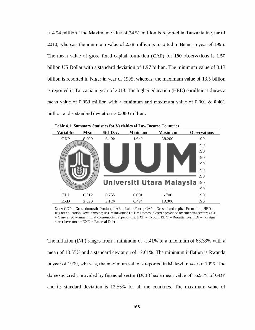
168
is 4.94 million. The Maximum value of 24.51 million is reported in Tanzania in year of
2013, whereas, the minimum value of 2.38 million is reported in Benin in year of 1995.
The mean value of gross fixed capital formation (CAP) for 190 observations is 1.50
billion US Dollar with a standard deviation of 1.97 billion. The minimum value of 0.13
billion is reported in Niger in year of 1995, whereas, the maximum value of 13.5 billion
is reported in Tanzania in year of 2013. The higher education (HED) enrollment shows a
mean value of 0.058 million with a minimum and maximum value of 0.001 & 0.461
million and a standard deviation is 0.080 million.
Table 4.1: Summary Statistics for Variables of Low Income Countries
Variables Mean Std. Dev. Minimum Maximum Observations
GDP 8.090 6.400 1.640 38.200 190
LAB 7.503 4.940 2.384 24.506 190
CAP 1.500 1.970 0.132 13.500 190
HED 0.058 0.080 0.001 0.461 190
INF 10.552 12.612 -2.406 83.326 190
DCF 16.909 13.564 1.739 69.068 190
GCE 0.941 1.060 0.133 7.240 190
EXP 1.580 1.690 0.067 9.500 190
REM 0.231 0.729 0.001 5.590 190
FDI 0.312 0.755 0.001 6.700 190
EXD 3.020 2.120 0.434 13.000 190
Note: GDP = Gross domestic Product; LAB = Labor Force; CAP = Gross fixed capital Formation; HED =
Higher education Development; INF = Inflation; DCF = Domestic credit provided by financial sector; GCE
= General government final consumption expenditure; EXP = Export; REM = Remittances; FDI = Foreign
direct investment; EXD = External Debt.
The inflation (INF) ranges from a minimum of -2.41% to a maximum of 83.33% with a
mean of 10.55% and a standard deviation of 12.61%. The minimum inflation is Rwanda
in year of 1999, whereas, the maximum value is reported in Malawi in year of 1995. The
domestic credit provided by financial sector (DCF) has a mean value of 16.91% of GDP
and its standard deviation is 13.56% for all the countries. The maximum value of
169
domestic credit provided by financial sector (DCF) of 69.07% is reported in Nepal in
year of 2009 and the minimum value of 1.74% is reported in Mozambique in year of
1996. General government final consumption expenditure (GCE) has a mean value of
0.94 billion US Dollar and the standard deviation is 1.06 billion. The maximum value of
7.24 billion is reported in Tanzania in year of 2013 and the minimum value of 0.13
billion is reported in Rwanda in year of 1995. The mean value of export for 190
observations is 1.58 billion US Dollar with a standard deviation of 1.69 billion. The
minimum values of 0.07 billion is reported in Rwanda in year of 1995 and the maximum
value of 9.50 billion is reported in Cambodia in year of 2013. The remittances (REM)
shows a mean value of 0.23 billion US Dollar with a minimum and maximum value of
0.001 & 5.59 billion and a standard deviation 0.73 billion. The maximum value is
reported in Nepal in year of 2013. The foreign direct investment (FDI) shows a mean
value of 0.31 billion US Dollar with a minimum and maximum value of 0.001 & 6.70
billion and a standard deviation 0.76 billion. The maximum value is reported in
Mozambique in year of 2013. The external debt (EXD) has a mean value of 3.02 billion
US Dollar and its standard deviation is 2.12 billion for all the countries. The maximum
value of external debt (EXD) of 13.00 billion is reported in Tanzania in year of 2013,
whereas, the minimum value of 0.43 billion is reported in Rwanda in year of 2006.
The Table 4.2 shows the properties of the variables of lower middle income countries.
The gross domestic product (GDP) has a mean value of 132.00 billion US Dollar for all
the countries in the sample and its standard deviation is 276.00 billion. The maximum
value of gross domestic product (GDP) is 2050.00 billion and the minimum value is

170
0.44 billion. Labor force (LAB) has a mean value of 37.30 million and the standard
deviation is 89.64 million. The Maximum value is 488.00 million and the minimum
value is 0.08 million. The mean value of gross fixed capital formation (CAP) for 437
observations is 25.10 billion US Dollar with a standard deviation of 73.20 billion and
minimum and maximum values of 0.04 and 618 billion respectively. The higher
education (HED) enrollment shows a mean value of 1.389 million with a minimum and
maximum value of 0.001 & 35.07 million and a standard deviation is 3.72 million.
Table 4.2: Summary Statistics for Variables of Lower Middle Income Countries
Variables Mean Std. Dev. Minimum Maximum Observations
GDP 132.000 276.000 0.440 2050.000 437
LAB 37.303 89.644 0.078 488.000 437
CAP 25.100 73.200 0.044 618.000 437
HED 1.389 3.720 0.001 35.071 437
INF 10.580 22.260 -0.791 376.746 437
DCF 40.287 22.744 1.819 112.677 437
GCE 11.000 25.900 0.044 210.000 437
EXP 24.900 55.700 0.098 468.000 437
REM 4.170 8.440 0.001 70.000 437
FDI 1.960 4.790 0.0004 43.400 437
EXD 30.200 53.700 0.048 430.000 437
Note: GDP = Gross domestic Product; LAB = Labor Force; CAP = Gross fixed capital Formation; HED =
Higher education Development; INF = Inflation; DCF = Domestic credit provided by financial sector; GCE
= General government final consumption expenditure; EXP = Export; REM = Remittances; FDI = Foreign
direct investment; EXD = External Debt.
The inflation (INF) ranges from a minimum of -0.79% to a maximum of 376.75% with a
mean of 10.58% and a standard deviation of 22.26%. The domestic credit provided by
financial sector (DCF) has a mean value of 40.29% of GDP and its standard deviation is
22.74% for all the countries. The maximum value of domestic credit provided by
financial sector (DCF) is 112.68% and the minimum value is 1.82%. General
government final consumption expenditure (GCE) has a mean value of 11.00 billion US

171
Dollar and the standard deviation is 25.90 billion. The Maximum value is 210 billion
and the minimum value is 0.04 billion. The mean value of export for 437 observations is
24.90 billion US Dollar with a standard deviation of 55.70 billion and minimum and
maximum values of 0.10 and 468.00 billion respectively. The remittances (REM) shows
a mean value of 4.17 billion US Dollar with a minimum and maximum value of 0.001 &
70.00 billion and a standard deviation of 8.44 billion. The foreign direct investment
(FDI) shows a mean value of 1.96 billion US Dollar with a minimum and maximum
value of 0.0004 & 43.40 billion and a standard deviation 4.79 billion. The external debt
(EXD) has a mean value of 30.20 billion US Dollar and its standard deviation is 53.70
billion for all the countries. The maximum value of external debt (EXD) is 430.00
billion and the minimum value is 0.05 billion.
The Table 4.3 shows the properties of the variables of upper middle income countries.
The gross domestic product (GDP) has a mean value of 301.00 billion US Dollar for all
the countries in the sample and its standard deviation is 827.00 billion. The maximum
value of gross domestic product (GDP) is 7670.00 billion and the minimum value is
0.45 billion. Labor force (LAB) has a mean value of 35.74 million and the standard
deviation is 134 million. The Maximum value is 802.00 billion and the minimum value
is 0.001 million. The mean value of gross fixed capital formation (CAP) for 570
observations is 74.30 billion US Dollar with a standard deviation of 341.00 billion and
minimum and maximum values of 0.08 and 4340 billion respectively. The higher
education (HED) enrollment shows a mean value of 0.669 million with a minimum and
maximum value of 0.001 & 7.614 million and a standard deviation is 1.045 million.

172
Table 4.3: Summary Statistics for Variables of Upper Middle Income Countries
Variables Mean Std. Dev. Minimum Maximum Observations
GDP 301.000 827.000 0.450 7670.000 570
LAB 35.741 134.000 0.0001 802.000 570
CAP 74.300 341.000 0.079 4340.000 570
HED 0.669 1.045 0.001 7.614 570
INF 13.783 59.382 -8.525 411.759 570
DCF 60.716 41.641 0.363 192.660 570
GCE 35.200 113.000 0.046 1290.000 570
EXP 66.300 203.000 0.124 2210.000 570
REM 1.810 3.780 0.001 26.900 570
FDI 7.750 27.100 0.007 291.000 570
EXD 52.000 98.600 0.117 871.000 570
Note: GDP = Gross domestic Product; LAB = Labor Force; CAP = Gross fixed capital Formation; HED =
Higher education Development; INF = Inflation; DCF = Domestic credit provided by financial sector; GCE
= General government final consumption expenditure; EXP = Export; REM = Remittances; FDI = Foreign
direct investment; EXD = External Debt.
The inflation (INF) ranges from a minimum of -8.53% to a maximum of 411.759% with
a mean of 13.78% and a standard deviation of 59.38%. The domestic credit provided by
financial sector (DCF) has a mean value of 60.72% of GDP and its standard deviation is
41.64% for all the countries. The maximum value of domestic credit provided by
financial sector (DCF) is 192.66% million and the minimum value is 0.36%. General
government final consumption expenditure (GCE) has a mean value of 35.20 billion US
Dollar and the standard deviation is 113.00 billion. The maximum value is 1290.00
billion and the minimum value is 0.05 billion. The mean value of export for 570
observations is 66.30 billion US Dollar with a standard deviation of 203 billion and
minimum and maximum values of 0.12 and 2210 billion respectively. The remittances
(REM) shows a mean value of 1.81 billion US Dollar with a minimum and maximum
value of 0.001 & 26.90 billion and a standard deviation of 3.78 billion. The foreign
direct investment (FDI) shows a mean value of 7.75 billion US Dollar with a minimum

173
and maximum value of 0.007 & 291.00 billion and a standard deviation of 27.10 billion.
The external debt (EXD) has a mean value of 52.00 billion US Dollar and its standard
deviation is 98.60 billion for all the countries. The maximum value of external debt
(EXD) is 871.00 billion and the minimum value is 0.12 billion.
Table 4.4: Summary Statistics for Variables of High Income Countries
Variables Mean Std. Dev. Minimum Maximum Observations
GDP 1170.000 2480.000 0.603 15800.000 627
LAB 17.537 29.515 0.0001 160.000 627
CAP 222.000 480.000 0.077 3200.000 627
HED 1.880 3.390 0.007 21.238 627
INF 5.036 10.307 -5.205 144.003 627
DCF 109.802 69.026 1.677 366.533 627
GCE 181.000 370.000 0.140 2540.000 627
EXP 235.000 337.000 0.053 2260.000 627
REM 2.300 3.300 0.000 24.400 627
FDI 24.700 58.800 0.009 734.000 627
Note: GDP = Gross domestic Product; LAB = Labor Force; CAP = Gross fixed capital Formation; HED =
Higher education Development; INF = Inflation; DCF = Domestic credit provided by financial sector; GCE
= General government final consumption expenditure; EXP = Export; REM = Remittances; FDI = Foreign
direct investment; EXD = External Debt.
The Table 4.4 shows the properties of the variables of high income countries. The gross
domestic product (GDP) has a mean value of 1170.00 billion US Dollar for all the
countries in the sample and its standard deviation is 2480.00 billion. The maximum
value of gross domestic product (GDP) is 15800.00 billion and the minimum value is
0.60 billion. Labor force (LAB) has a mean value of 17.54 million and the standard
deviation is 29.51 million. The maximum value is 160.00 million and the minimum
value is 0.001 million. The mean value of gross fixed capital formation (CAP) for 627
observations is 222 billion US Dollar with a standard deviation of 480 billion and
minimum and maximum values of 0.08 and 3200 billion respectively. The higher
174
education (HED) enrollment shows a mean value of 1.88 million with a minimum and
maximum value of 0.007 & 21.238 million and a standard deviation is 3.390 million.
The inflation (INF) ranges from a minimum of -5.20% to a maximum of 144% with a
mean of 5.04% and a standard deviation of 10.31%. The domestic credit provided by
financial sector (DCF) has a mean value of 109.80% and its standard deviation is
69.03% of GDP for all the countries. The maximum value of domestic credit provided
by financial sector (DCF) is 366.53% and the minimum value is 1.68%. General
government final consumption expenditure (GCE) has a mean value of 181.00 billion
US Dollar and the standard deviation is 370.00 billion. The maximum value is 2540.00
billion and the minimum value is 0.14 billion.The mean value of export for 627
observations is 235.00 billion US Dollar with a standard deviation of 337.00 billion and
minimum and maximum values of 0.05 and 2260.00 billion respectively. The
remittances (REM) shows a mean value of 2.30 billion US Dollar with a minimum and
maximum value of 0 & 24.40 billion and a standard deviation of 3.30 billion. The
foreign direct investment (FDI) shows a mean value of 24.70 billion US Dollar with a
minimum and maximum value of 0.01 & 734.00 billion and a standard deviation of
58.80 billion.
The Table 4.5 shows the properties of the variables of the aggreagate sample of 96
countries all together. The gross domestic product (GDP) has a mean value of 529.00
billion US Dollar for all the countries in the sample and its standard deviation is 1600.00
billion. The maximum value of gross domestic product (GDP) of 15800.00 billion is

175
reported in United States of America in year of 2013 from high income category,
whereas, the minimum value of 0.44 billion is reported in Vanuatu in year of 1995 from
the lower middle income category. Labor force (LAB) has a mean value of 26.92
million and the standard deviation is 89.26 million. The maximum value of 802 million
is reported in China in year of 2013 from the upper middle income category and the
minimum value is 53.96 thousands is reported in Grenada in year of 1995 from the
upper middle income category.
The mean value of gross fixed capital formation (CAP) for 1844 observations is 106.00
billion US Dollar with a standard deviation of 352.00 billion and minimum and
maximum values of 0.04 and 4340.00 billion respectively. The maximum value is
reported in China in year of 2013 from the upper middle income category. The
minimum value is reported in Vanuatu in year of 1998 from the lower middle income
category. The higher education (HED) enrollment shows a mean value of 0.999 million
with a minimum and maximum value of 0.001 & 35.071 million and a standard
deviation is 2.059 million.
The inflation (INF) ranges from a minimum of -8.53% to a maximum of 411.759% with
a mean of 9.67% and a standard deviation of 35.85%. The maximum value is reported in
Bulgaria in year of 1997 from the upper middle income category. The minimum value is
reported in Azerbaijan in year of 1999 from the upper middle income category. The
domestic credit provided by financial sector (DCF) has a mean value of 68.13% of GDP
and its standard deviation is 58.26% for all the countries. The maximum value of
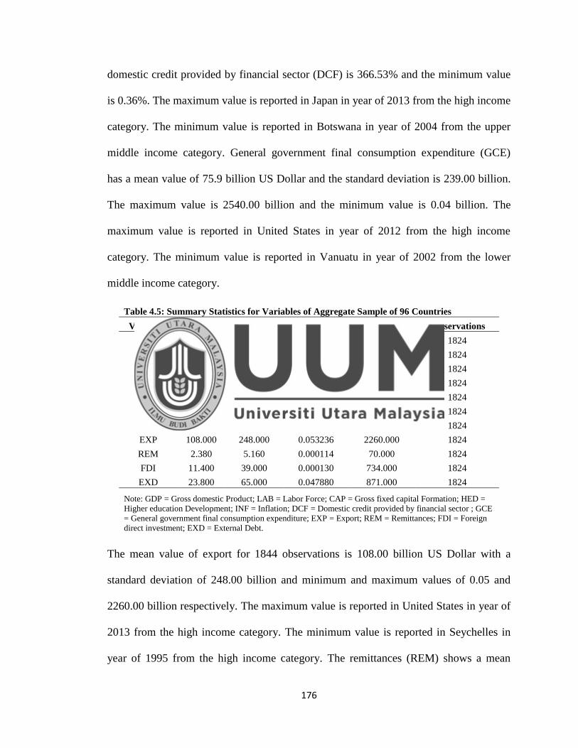
176
domestic credit provided by financial sector (DCF) is 366.53% and the minimum value
is 0.36%. The maximum value is reported in Japan in year of 2013 from the high income
category. The minimum value is reported in Botswana in year of 2004 from the upper
middle income category. General government final consumption expenditure (GCE)
has a mean value of 75.9 billion US Dollar and the standard deviation is 239.00 billion.
The maximum value is 2540.00 billion and the minimum value is 0.04 billion. The
maximum value is reported in United States in year of 2012 from the high income
category. The minimum value is reported in Vanuatu in year of 2002 from the lower
middle income category.
Table 4.5: Summary Statistics for Variables of Aggregate Sample of 96 Countries
Variables Mean Std. Dev. Minimum Maximum Observations
GDP 529.000 1600.000 0.440000 15800.000 1824
LAB 26.916 89.264 0.000054 802.000 1824
CAP 106.000 352.000 0.043963 4340.000 1824
HED 0.999 2.059 0.000600 35.071 1824
INF 9.672 35.848 -8.525170 411.759 1824
DCF 68.132 58.257 0.362724 366.533 1824
GCE 75.900 239.000 0.043693 2540.000 1824
EXP 108.000 248.000 0.053236 2260.000 1824
REM 2.380 5.160 0.000114 70.000 1824
FDI 11.400 39.000 0.000130 734.000 1824
EXD 23.800 65.000 0.047880 871.000 1824
Note: GDP = Gross domestic Product; LAB = Labor Force; CAP = Gross fixed capital Formation; HED =
Higher education Development; INF = Inflation; DCF = Domestic credit provided by financial sector ; GCE
= General government final consumption expenditure; EXP = Export; REM = Remittances; FDI = Foreign
direct investment; EXD = External Debt.
The mean value of export for 1844 observations is 108.00 billion US Dollar with a
standard deviation of 248.00 billion and minimum and maximum values of 0.05 and
2260.00 billion respectively. The maximum value is reported in United States in year of
2013 from the high income category. The minimum value is reported in Seychelles in
year of 1995 from the high income category. The remittances (REM) shows a mean

177
value of 2.38 billion US Dollar with a minimum and maximum value of 0.00011 &
70.00 billion and a standard deviation of 5.16 billion. The maximum value is reported in
India in year of 2013 from the lower middle income category. The foreign direct
investment (FDI) shows a mean value of 11.40 billion US Dollar with a minimum and
maximum value of 0.00013 & 734.00 billion and a standard deviation of 39.00 billion.
The maximum value is reported in Netherlands in year of 2007 from the high income
category. The external debt (EXD) has a mean value of 23.80 billion US Dollar and its
standard deviation is 65.00 billion for all the countries. The maximum value of external
debt (EXD) is 871.00 billion and the minimum value is 0.0479 billion.
4.3 Low Income Countries
In this section, we present the results of empirical estimations of low income countries
and further discuss these results in the theoretical and conceptual context.
4.3.1 Unit Root Analyses
Table 4.6: Results of Stationary Analyses for Low Income Countries
Variables
Im, Pesaran and Shin
I(0) I(1)
C C&T C C&T
GDP 14.427 5.399 -2.142** -6.960*
LAB 24.773 6.436 -2.593* -3.133*
CAP 7.828 2.791 -6.526* -7.650*
HED 3.497 1.022 -2.796* -2.595*
INF 11.809 3.570 -13.173* -7.733*
DCF 6.182 1.267 -6.698* -6.475*
GCE 7.770 1.298 -6.330* -5.968*
FDI 4.612 -0.434 -10.108* -6.779*
EXP 0.868 1.258 -8.701* -7.699*
REM 4.491 -0.596 -9.061* -6.931*
EXD 2.240 2.324 -7.577* -6.388*
*, **, *** indicates significance level respectively at 1%, 5% and 10%.
Source: Author‘s estimation.
178
We use, Im, Pesaran and Shin (2003) unit root test to analyze the stationary properties of
our considered variables. The IPS test considers the unobserved heterogeneity among
the cross sections and also eliminates the issues of serial correlation. The IPS unit root
test has the best properties to judge the problem of a unit root in the small sample. The
desirable results for unit root test include that the variables should be non-stationary at
the level and become stationary at the first difference. Table 4.6 represents the results of
stationary analyses for low income countries. We first, employed these tests on the level
of each variable and then applied to the first difference. In both estimation procedures of
level and first difference, we also analyze the results in two dimensions, i.e. with
constant and with constant and trend. Results indicate that all the variables are non-
stationary at level and become stationary at first difference. These results confirm that
there is no problem of unit root in our variables of low income countries and we can
further use these variables for the long run estimations.
4.3.2 Cointegration Analyses
After having the confirmation from unit root test that our variables have a stationary
properties of I(1) which is the requirement to perform panel cointegration techniques,
we applied two methods of panel cointegration i.e. Pedroni cointegration (1999) and
Kao cointegration (1999) to analyze the long run relationship among foreign capital
inflows, banking crisis, currency crisis and economic growth in low income countries.
These tests are based on the two-step residual based cointegration tests of Engle-
Granger (1987). The Pedroni cointegration based on a seven statistical value. The
Pedroni cointegration is useful to control the biasness of country size and also solve the

179
issues of heterogeneity (Das & Choudhary, 2011). The Kao cointegration method
follows the same basic approached as used in the Pedroni cointegration, but also control
the issues of cross-section specific intercepts and homogenous coefficients.
Table 4.7: Results of Pedroni ((Engle-Granger based) Panel Cointegration in Low Income Countries
Estimates Stats. Prob.
GDP = f (LAB+CAP+HED+INF+DCF+GCE+BAC)
Panel v-statistic -0.583 0.720
Panel rho-statistic 1.875 0.970
Panel PP statistic -1.700 0.045
Panel ADF statistic -1.765 0.039
Alternative Hypothesis: Individual AR Coefficient
Group rho-statistic 2.398 0.992
Group PP statistic -2.477 0.007
Group ADF statistic -1.577 0.057
GDP = f (LAB+CAP+HED+INF+DCF+GCE+CRC)
Panel v-statistic 0.592 0.277
Panel rho-statistic 3.704 1.000
Panel PP statistic -1.505 0.066
Panel ADF statistic -3.096 0.001
Alternative Hypothesis: Individual AR Coefficient
Group rho-statistic 5.043 1.000
Group PP statistic -2.457 0.007
Group ADF statistic -3.249 0.001
GDP = f (LAB+CAP+HED+INF+DCF+GCE+FDI)
Panel v-statistic 1.379 0.084
Panel rho-statistic 2.496 0.994
Panel PP statistic -5.020 0.000
Panel ADF statistic -5.032 0.000
Alternative Hypothesis: Individual AR Coefficient
Group rho-statistic 4.215 1.000
Group PP statistic -5.485 0.000
Group ADF statistic -5.691 0.000
GDP = f (LAB+CAP+HED+INF+DCF+GCE+EXP)
Panel v-statistic -0.741 0.771
Panel rho-statistic 3.088 0.999
Panel PP statistic -2.723 0.003
Panel ADF statistic -3.825 0.000
Alternative Hypothesis: Individual AR Coefficient
Group rho-statistic 4.512 1.000
Group PP statistic -4.338 0.000
Group ADF statistic -3.607 0.000
GDP = f (LAB+CAP+HED+INF+DCF+GCE+REM)
Panel v-statistic 0.660 0.255
Panel rho-statistic 3.391 1.000
Panel PP statistic -2.544 0.006
Panel ADF statistic -3.449 0.000
Alternative Hypothesis: Individual AR Coefficient
Group rho-statistic 4.758 1.000
Group PP statistic -3.689 0.000
Group ADF statistic -3.526 0.000
GDP = f (LAB+CAP+HED+INF+DCF+GCE+EXD)
Panel v-statistic 0.895 0.186
Panel rho-statistic 3.271 1.000
Panel PP statistic -3.017 0.001
Panel ADF statistic -3.953 0.000

180
Alternative Hypothesis: Individual AR Coefficient
Group rho-statistic 4.805 1.000
Group PP statistic -2.924 0.002
Group ADF statistic -3.649 0.000
The null hypothesis of Pedroni's (1997) panel cointegration procedure is no cointegration Source: Author‘s estimation.
Table 4.8: Results of Pedroni ((Engle-Granger based) Panel Cointegration of Interaction Terms in Low Income Countries
Estimates Stats. Prob. Stats. Prob.
GDP = f
(LAB+CAP+HED+INF+DCF+GCE+FDI*BAC)
GDP = f
(LAB+CAP+HED+INF+DCF+GCE+FDI*CRC)
Panel v-statistic -1.033 0.849 0.339 0.367
Panel rho-statistic 1.711 0.957 3.463 1.000
Panel PP statistic -1.872 0.031 -3.489 0.000
Panel ADF statistic -1.756 0.040 -3.072 0.001
Alternative Hypothesis: Individual AR Coefficient
Group rho-statistic 2.242 0.988 4.612 1.000
Group PP statistic -3.986 0.000 -4.983 0.000
Group ADF statistic -1.818 0.035 -3.096 0.001
GDP = f
(LAB+CAP+HED+INF+DCF+GCE+EXP*BAC)
GDP = f
(LAB+CAP+HED+INF+DCF+GCE+EXP*CRC)
Panel v-statistic -1.023 0.847 0.303 0.381
Panel rho-statistic 1.673 0.953 3.494 1.000
Panel PP statistic -1.916 0.028 -3.340 0.000
Panel ADF statistic -2.003 0.023 -3.099 0.001
Alternative Hypothesis: Individual AR Coefficient
Group rho-statistic 2.198 0.986 4.657 1.000
Group PP statistic -4.047 0.000 -4.667 0.000
Group ADF statistic -2.506 0.006 -2.928 0.002
GDP = f
(LAB+CAP+HED+INF+DCF+GCE+REM*BAC)
GDP = f
(LAB+CAP+HED+INF+DCF+GCE+REM*CRC)
Panel v-statistic -1.020 0.846 0.298 0.383
Panel rho-statistic 1.690 0.954 3.501 1.000
Panel PP statistic -1.822 0.034 -3.306 0.001
Panel ADF statistic -1.910 0.028 -3.112 0.001
Alternative Hypothesis: Individual AR Coefficient
Group rho-statistic 2.218 0.987 4.661 1.000
Group PP statistic -3.982 0.000 -4.636 0.000
Group ADF statistic -2.441 0.007 -2.947 0.002
GDP = f
(LAB+CAP+HED+INF+DCF+GCE+EXD*BAC)
GDP = f
(LAB+CAP+HED+INF+DCF+GCE+EXD*CRC)
Panel v-statistic -1.023 0.847 0.313 0.377
Panel rho-statistic 1.674 0.953 3.484 1.000
Panel PP statistic -1.911 0.028 -3.373 0.000
Panel ADF statistic -1.998 0.023 -3.108 0.001
Alternative Hypothesis: Individual AR Coefficient
Group rho-statistic 2.199 0.986 4.655 1.000
Group PP statistic 2.199 0.986 -4.681 0.000
Group ADF statistic 2.199 0.986 -2.920 0.002
The null hypothesis of Pedroni's (1997) panel cointegration procedure is no cointegration
Source: Author's estimation.

181
Results of Pedroni cointegration are reported in Table 4.7 and 4.8, while the results of
Kao cointegration are reported in Table 4.9. The results of Pedroni cointegration method
indicate the rejection of null hypothesis of no cointegration for the all test statistics at
10% or better level of significance except the panel v-statistics and rho-statistics.
According to Pedroni (2004), Al-Irani (2006) and Pao & Tsai (2010) in small time
dimensions, the panel v-statistics and rho-statistics may have a very low power.
Furthermore, Guterrez (2003) concludes that group statistics (especially Augmented
Dickey Fuller (ADF) and Phillips and Perron (PP) have the best power to judge the long
run cointegration among the test statistics of Pedroni (1999). Therefore, we can
conclude that the foreign capital inflows, banking crisis, currency crisis and economic
growth are cointegrated in the long run in the sample of low income countries. Results
of Kao cointegration are reported in Table 4.9.
Table 4.9: Results of Kao (Engle-Granger based) Panel Cointegration in Low Income Countries
Estimates Stats. Prob.
GDP = f (LAB+CAP+HED+INF+DCF+GCE+BAC)
Panel ADF statistic -3.326 0.000
GDP = f (LAB+CAP+HED+INF+DCF+GCE+CRC)
Panel ADF statistic -3.720 0.000
GDP = f (LAB+CAP+HED+INF+DCF+GCE+FDI)
Panel ADF statistic -3.715 0.000
GDP = f (LAB+CAP+HED+INF+DCF+GCE+EXP)
Panel ADF statistic -3.316 0.001
GDP = f (LAB+CAP+HED+INF+DCF+GCE+REM)
Panel ADF statistic -3.630 0.000
GDP = f (LAB+CAP+HED+INF+DCF+GCE+EXD)
Panel ADF statistic -3.983 0.000
GDP = f (LAB+CAP+HED+INF+DCF+GCE+FDI*BAC)
Panel ADF statistic -3.314 0.001
GDP = f (LAB+CAP+HED+INF+DCF+GCE+FDI*CRC)
Panel ADF statistic -3.734 0.000
GDP = f (LAB+CAP+HED+INF+DCF+GCE+EXP*BAC)
Panel ADF statistic -3.390 0.000
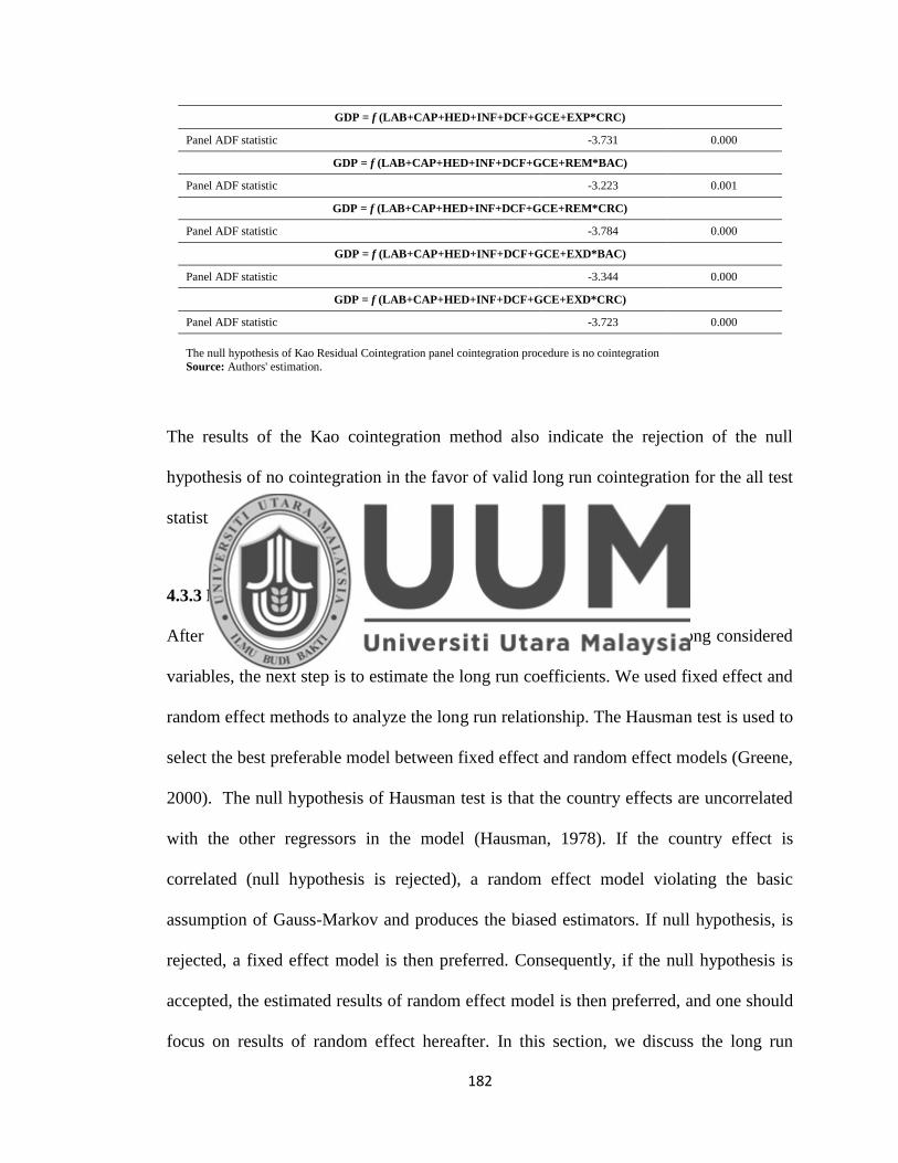
182
GDP = f (LAB+CAP+HED+INF+DCF+GCE+EXP*CRC)
Panel ADF statistic -3.731 0.000
GDP = f (LAB+CAP+HED+INF+DCF+GCE+REM*BAC)
Panel ADF statistic -3.223 0.001
GDP = f (LAB+CAP+HED+INF+DCF+GCE+REM*CRC)
Panel ADF statistic -3.784 0.000
GDP = f (LAB+CAP+HED+INF+DCF+GCE+EXD*BAC)
Panel ADF statistic -3.344 0.000
GDP = f (LAB+CAP+HED+INF+DCF+GCE+EXD*CRC)
Panel ADF statistic -3.723 0.000
The null hypothesis of Kao Residual Cointegration panel cointegration procedure is no cointegration
Source: Authors' estimation.
The results of the Kao cointegration method also indicate the rejection of the null
hypothesis of no cointegration in the favor of valid long run cointegration for the all test
statistics at the 1 % level of significance in low income countries.
4.3.3 Long Run Analysis
After having the valid evidence of significant long run cointegration among considered
variables, the next step is to estimate the long run coefficients. We used fixed effect and
random effect methods to analyze the long run relationship. The Hausman test is used to
select the best preferable model between fixed effect and random effect models (Greene,
2000). The null hypothesis of Hausman test is that the country effects are uncorrelated
with the other regressors in the model (Hausman, 1978). If the country effect is
correlated (null hypothesis is rejected), a random effect model violating the basic
assumption of Gauss-Markov and produces the biased estimators. If null hypothesis, is
rejected, a fixed effect model is then preferred. Consequently, if the null hypothesis is
accepted, the estimated results of random effect model is then preferred, and one should
focus on results of random effect hereafter. In this section, we discuss the long run

183
impact and coefficients of different independent variables on economic growth in the
sample of low income countries.
Banking Crisis and Currency Crisis
The results which explain the long run impact of banking crisis and currency crisis on
economic growth is presented in Table 4.10. The results of banking crisis are reported in
model I whereas, the results of currency crisis are reported in model II. Results of both
models indicate that the prob. value of Hausman test is insignificant (0.963) and (0.211),
which confirm the acceptance of null hypothesis and concluded that the random effect
model is preferred over fixed effect model. Furthermore, the statistical value of Variance
Inflation factor (VIF) also suggest that there is no issue of multicollinearity exist among
the independent variables of estimated models. Results also indicate the negative and
significant impact of banking crisis on economic growth, whereas, the negative, but
insignificant influence of currency crisis on economic growth is observed. It is
concluded that the banking and currency crises decrease the progress of the economic
development. Results also conclude that the banking crises is more harmful to the
economic growth of low income countries as compare to currency crises.
Furthermore, the results of control variables show that the labor force, capital formation,
higher education development, domestic credit by financial sector and government
consumption expenditure have significant positive impact on economic growth whereas,
inflation has significant negative impact on economic growth in low income countries.
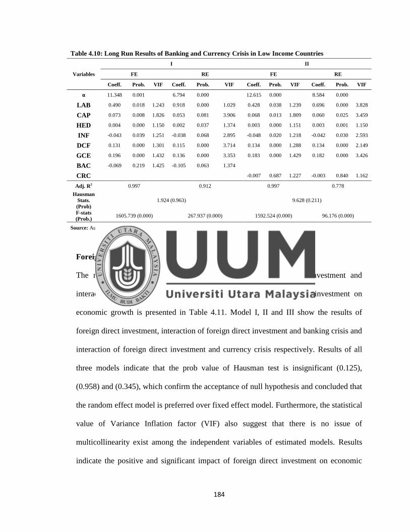
184
Table 4.10: Long Run Results of Banking and Currency Crisis in Low Income Countries
Variables
I II
FE RE FE RE
Coeff. Prob. VIF Coeff. Prob. VIF Coeff. Prob. VIF Coeff. Prob. VIF
α 11.348 0.001
6.794 0.000
12.615 0.000
8.584 0.000
LAB 0.490 0.018 1.243 0.918 0.000 1.029 0.428 0.038 1.239 0.696 0.000 3.828
CAP 0.073 0.008 1.826 0.053 0.081 3.906 0.068 0.013 1.809 0.060 0.025 3.459
HED 0.004 0.000 1.150 0.002 0.037 1.374 0.003 0.000 1.151 0.003 0.001 1.150
INF -0.043 0.039 1.251 -0.038 0.068 2.895 -0.048 0.020 1.218 -0.042 0.030 2.593
DCF 0.131 0.000 1.301 0.115 0.000 3.714 0.134 0.000 1.288 0.134 0.000 2.149
GCE 0.196 0.000 1.432 0.136 0.000 3.353 0.183 0.000 1.429 0.182 0.000 3.426
BAC -0.069 0.219 1.425 -0.105 0.063 1.374
CRC -0.007 0.687 1.227 -0.003 0.840 1.162
Adj. R2 0.997 0.912 0.997 0.778
Hausman
Stats.
(Prob)
1.924 (0.963) 9.628 (0.211)
F-stats
(Prob.) 1605.739 (0.000) 267.937 (0.000) 1592.524 (0.000) 96.176 (0.000)
Source: Authors' estimation.
Foreign Direct Investment
The results which explain the long run impact of foreign direct investment and
interaction terms of banking and currency crisis with foreign direct investment on
economic growth is presented in Table 4.11. Model I, II and III show the results of
foreign direct investment, interaction of foreign direct investment and banking crisis and
interaction of foreign direct investment and currency crisis respectively. Results of all
three models indicate that the prob value of Hausman test is insignificant (0.125),
(0.958) and (0.345), which confirm the acceptance of null hypothesis and concluded that
the random effect model is preferred over fixed effect model. Furthermore, the statistical
value of Variance Inflation factor (VIF) also suggest that there is no issue of
multicollinearity exist among the independent variables of estimated models. Results
indicate the positive and significant impact of foreign direct investment on economic

185
growth. The coefficient of foreign direct investment is showing that the 1% increase in
FDI causes the increase in economic growth by 0.008%. This finding is consistent with
the previous empirical studies of (Vudayagiri N Balasubramanyam et al., 1999;
Nair‐Reichert and Weinhold, 2001; Choe, 2003; Li and Liu, 2005; Rabiei and Masoudi,
2012; Omri and Kahouli, 2014; Olayemi, 2015; Yusoff and Nuh, 2015). Results of
model II and III confirm that the impact of foreign direct investment on economic
growth becomes negative and insignificant in the presence of systemic banking crises
and currency crises. Results further conclude that the systemic banking crisis (-0.007)
comparatively more effects the influence of FDI on economic growth as compared to
currency crisis (-0.004) in low income countries.
Furthermore, the results of control variables show that the labor force, capital formation,
higher education development, domestic credit by the financial sector and government
consumption expenditure have a positive impact on economic growth whereas, inflation
has negative impact on economic growth in low income countries.
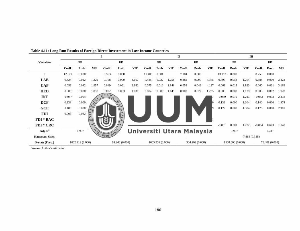
186
Table 4.11: Long Run Results of Foreign Direct Investment in Low Income Countries
Variables
I II III
FE RE FE RE FE RE
Coeff. Prob. VIF Coeff. Prob. VIF Coeff. Prob. VIF Coeff. Prob. VIF Coeff. Prob. VIF Coeff. Prob. VIF
α 12.529 0.000
8.563 0.000
11.403 0.001
7.104 0.000
13.013 0.000
8.750 0.000
LAB 0.424 0.022 1.220 0.708 0.000 4.167 0.488 0.022 1.258 0.882 0.000 3.365 0.407 0.058 1.264 0.684 0.000 3.423
CAP 0.059 0.042 1.957 0.049 0.091 3.862 0.075 0.010 1.846 0.058 0.046 4.117 0.068 0.018 1.823 0.060 0.031 3.163
HED 0.003 0.000 1.057 0.002 0.003 1.081 0.004 0.000 1.145 0.002 0.022 1.235 0.003 0.000 1.129 0.003 0.002 1.120
INF -0.047 0.004 1.202 -0.042 0.031 2.599 -0.043 0.040 1.233 -0.039 0.062 2.707 -0.049 0.019 1.213 -0.042 0.032 2.238
DCF 0.138 0.000 1.295 0.136 0.000 2.152 0.135 0.000 1.309 0.115 0.000 2.340 0.139 0.000 1.304 0.140 0.000 1.974
GCE 0.186 0.000 1.360 0.177 0.000 3.441 0.187 0.000 1.370 0.143 0.000 4.229 0.172 0.000 1.384 0.175 0.000 2.901
FDI 0.008 0.082 1.125 0.007 0.030 1.323
FDI * BAC
-0.005 0.152 1.389 -0.007 0.050 1.281
FDI * CRC -0.001 0.501 1.222 -0.004 0.673 1.140
Adj. R2 0.997 0.779 0.997 0.917 0.997 0.739
Hausman. Stats. 11.336 (0.125) 2.029 (0.958) 7.864 (0.345)
F-stats (Prob.) 1602.919 (0.000) 91.946 (0.000) 1605.339 (0.000) 304.262 (0.000) 1588.806 (0.000) 73.481 (0.000)
Source: Author's estimation.
187
Export of Goods and Services
The results which explain the long run impact of exports of goods and services and
interaction terms of banking and currency crisis with exports of goods and services on
economic growth is presented in Table 4.12. Model I, II and III show the results of exports
of goods and services, interaction of exports and banking crisis and interaction of exports and
currency crisis respectively. Results of all three models indicate that the prob value of
Hausman test is insignificant (0.388), (0.953) and (0.187), which confirm the acceptance
of null hypothesis and concluded that the random effect model is preferred over fixed
effect model. Furthermore, the statistical value of Variance Inflation factor (VIF) also
suggest that there is no issue of multicollinearity exist among the independent variables
of estimated models. Results indicate the positive and significant impact of exports of
goods and services on economic growth. The coefficient of exports of goods and services
is showing that the 1% increase in exports causes the increase in economic growth by 0.266%.
This finding is consistent with the previous empirical studies. Results of model II confirm that
the impact of exports on economic growth becomes significantly negative in the presence of
systemic banking crises. Results of model III further confirm that the impact of export of goods
and service on economic growth becomes insignificant in the presence of currency crises. These
findings conclude that the banking and currency crisis are harmful to the relationship of export
and economic growth in low income countries.
Furthermore, the results of control variables show that the labor force, capital formation,
higher education development, domestic credit by the financial sector and government
consumption expenditure have a positive impact on economic growth whereas, inflation
has negative impact on economic growth in low income countries.
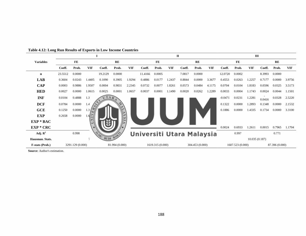
188
Table 4.12: Long Run Results of Exports in Low Income Countries
Variables
I II III
FE RE FE RE FE RE
Coeff. Prob. VIF Coeff. Prob. VIF Coeff. Prob. VIF Coeff. Prob. VIF Coeff. Prob. VIF Coeff. Prob. VIF
α 23.5512 0.0000
19.2129 0.0000
11.4166 0.0005
7.0817 0.0000
12.0720 0.0002
8.3993 0.0000
LAB 0.3604 0.0243 1.4405 0.1090 0.3905 1.9294 0.4886 0.0177 1.2437 0.8844 0.0000 3.3677 0.4553 0.0263 1.2257 0.7177 0.0000 3.9756
CAP 0.0003 0.9886 1.9507 0.0004 0.9831 2.2345 0.0732 0.0077 1.8261 0.0573 0.0484 4.1175 0.0704 0.0104 1.8183 0.0596 0.0325 3.5173
HED 0.0027 0.0000 1.0615 0.0025 0.0001 1.0657 0.0037 0.0001 1.1490 0.0020 0.0262 1.2289 0.0033 0.0004 1.1743 0.0024 0.0044 1.1501
INF 0.0104 0.4888 1.3239 0.0155 0.2956 1.5755 -0.0436 0.0363 1.2534 -0.0392 0.0599 2.7008 -0.0471 0.0231 1.2281 -
0.0416 0.0328 2.5220
DCF 0.0784 0.0000 1.4157 0.0843 0.0000 1.5358 0.1301 0.0000 1.3004 0.1142 0.0000 2.3390 0.1322 0.0000 1.2893 0.1348 0.0000 2.1532
GCE 0.1250 0.0000 1.3589 0.1500 0.0000 1.6750 0.1950 0.0000 1.4364 0.1436 0.0001 4.2217 0.1886 0.0000 1.4335 0.1734 0.0000 3.3100
EXP 0.2658 0.0000 1.6254 0.2512 0.0000 1.9306
EXP * BAC
-0.0032 0.2458 1.4331 -0.0049 0.0770 1.2841
EXP * CRC 0.0024 0.6933 1.2611 0.0015 0.7965 1.1704
Adj. R2 0.998 0.749 0.997 0.917 0.997 0.771
Hausman. Stats. 7.408 (0.388) 2.106 (0.953) 10.035 (0.187)
F-stats (Prob.) 3291.129 (0.000) 81.994 (0.000) 1619.315 (0.000) 304.453 (0.000) 1607.523 (0.000) 87.396 (0.000)
Source: Author's estimation.

189
Workers’ Remittances
The results which explain the long run impact of workers‘ remittances and interaction
terms of banking and currency crisis with workers‘ remittances on economic growth is
presented in Table 4.13. Model I, II and III show the results of workers‘ remittances,
interaction of workers‘ remittances and banking crisis and interaction of workers‘
remittances and currency crisis respectively. Results of all three models indicate that the
prob value of Hausman test is insignificant (0.697), (0.144) and (0.258), which confirm
the acceptance of null hypothesis and concluded that the random effect model is
preferred over fixed effect model. Furthermore, the statistical value of Variance
Inflation factor (VIF) also suggest that there is no issue of multicollinearity exist among
the independent variables of estimated models. Results indicate the negative, but
insignificant impact of workers‘ remittances on economic growth. This finding is
consistent with the previous empirical studies. Results of model II confirm that the impact of
workers‘ remittances on economic growth becomes significantly negative in the presence of
systemic banking crises. Results of model III further confirm that the impact of workers‘
remittances on economic growth becomes insignificant in the presence of currency crises.
These findings conclude that the banking and currency crisis are harmful to the relationship of
workers‘ remittances and economic growth in low income countries.
Furthermore, the results of control variables show that the labor force, capital formation,
higher education development, domestic credit by the financial sector and government
consumption expenditure have a positive impact on economic growth whereas, inflation
has negative impact on economic growth in low income countries.

190
Table 4.13: Long Run Results of Remittances in Low Income Countries
Variables
I II III
FE RE FE RE FE RE
Coeff. Prob. VIF Coeff. Prob. VIF Coeff. Prob. VIF Coeff. Prob. VIF Coeff. Prob. VIF Coeff. Prob. VIF
α 14.839 0.000
9.756 0.000
11.341 0.001
7.270 0.000
12.757 0.000
8.678 0.000
LAB 0.328 0.132 1.306 0.605 0.000 2.173 0.493 0.021 1.257 0.857 0.000 3.657 0.421 0.042 1.241 0.688 0.000 3.657
CAP 0.076 0.009 1.819 0.069 0.013 2.417 0.075 0.009 1.843 0.057 0.037 3.353 0.068 0.014 1.809 0.060 0.025 3.353
HED 0.003 0.000 1.063 0.003 0.001 1.069 0.004 0.000 1.147 0.003 0.003 1.133 0.004 0.000 1.133 0.003 0.001 1.133
INF -0.050 0.016 1.207 -0.041 0.034 1.641 -0.043 0.040 1.228 -0.040 0.043 2.499 -0.048 0.019 1.217 -0.042 0.030 2.499
DCF 0.129 0.000 1.374 0.140 0.000 1.586 0.134 0.000 1.311 0.113 0.000 2.086 0.134 0.000 1.286 0.135 0.000 2.086
GCE 0.164 0.000 1.453 0.183 0.000 1.970 0.187 0.000 1.360 0.159 0.000 3.281 0.182 0.000 1.425 0.183 0.000 3.281
REM 0.016 0.097 1.290 0.008 0.040 1.067
REM * BAC
-0.006 0.110 1.366 -0.008 0.025 1.134
REM * CRC -0.001 0.563 1.208 -0.004 0.696 1.134
Adj. R2 0.997 0.624 0.997 0.769 0.997 0.769
Hausman. Stats. 4.694 (0.697) 10.886 (0.144) 8.929 (0.258)
F-stats (Prob.) 1612.776 (0.000) 43.181 (0.000) 1610.589 (0.000) 91.489 (0.000) 1594.212 (0.000) 91.489 (0.000)
Source: Author's estimation.

191
External Debt
The results which explain the long run impact of external debt and interaction terms of
banking and currency crisis with external debt on economic growth is presented in Table
4.14. Model I, II and III show the results of external debt, interaction of external debt
and banking crisis and interaction of external debt and currency crisis respectively.
Results of all three models indicate that the prob value of Hausman test is insignificant
(0.999), (0.999) and (0.349), which confirm the acceptance of null hypothesis and
concluded that the random effect model is preferred over fixed effect model.
Furthermore, the statistical value of Variance Inflation factor (VIF) also suggest that
there is no issue of multicollinearity exist among the independent variables of estimated
models. Results indicate the positive and significant impact of external debt on
economic growth. This finding is consistent with the previous empirical studies. The
coefficient of external debt is showing that the 1% increase in external debt causes the
increase in economic growth by 0.076%. Results of model II confirm that the impact of
external debt on economic growth becomes significantly negative in the presence of
systemic banking crises. Results of model III further confirm that the impact of external
debt on economic growth becomes insignificant in the presence of currency crises.
These findings conclude that the banking and currency crisis are harmful for the
relationship of external debt and economic growth in low income countries.
Furthermore, the results of control variables show that the labor force, capital formation,
higher education development, domestic credit by the financial sector and government
consumption expenditure have a positive impact on economic growth whereas, inflation
has negative impact on economic growth in low income countries.
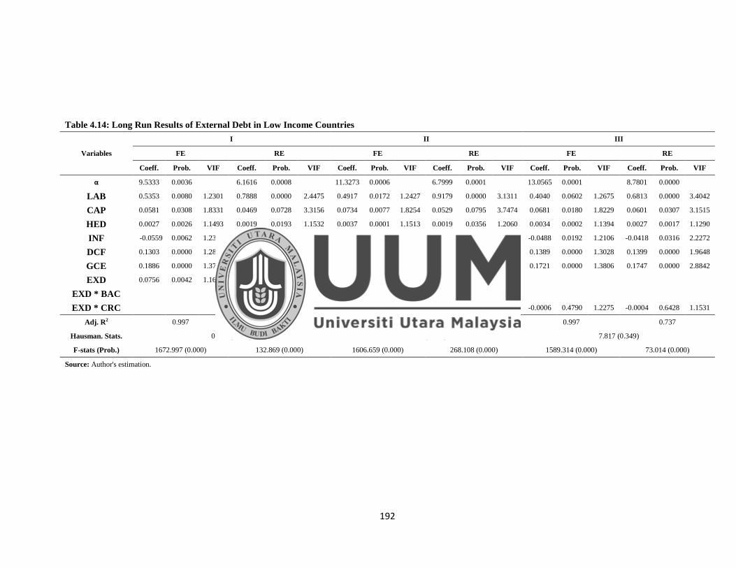
192
Table 4.14: Long Run Results of External Debt in Low Income Countries
Variables
I II III
FE RE FE RE FE RE
Coeff. Prob. VIF Coeff. Prob. VIF Coeff. Prob. VIF Coeff. Prob. VIF Coeff. Prob. VIF Coeff. Prob. VIF
α 9.5333 0.0036
6.1616 0.0008
11.3273 0.0006
6.7999 0.0001
13.0565 0.0001
8.7801 0.0000
LAB 0.5353 0.0080 1.2301 0.7888 0.0000 2.4475 0.4917 0.0172 1.2427 0.9179 0.0000 3.1311 0.4040 0.0602 1.2675 0.6813 0.0000 3.4042
CAP 0.0581 0.0308 1.8331 0.0469 0.0728 3.3156 0.0734 0.0077 1.8254 0.0529 0.0795 3.7474 0.0681 0.0180 1.8229 0.0601 0.0307 3.1515
HED 0.0027 0.0026 1.1493 0.0019 0.0193 1.1532 0.0037 0.0001 1.1513 0.0019 0.0356 1.2060 0.0034 0.0002 1.1394 0.0027 0.0017 1.1290
INF -0.0559 0.0062 1.2357 -0.0483 0.0116 2.0891 -0.0430 0.0392 1.2503 -0.0384 0.0682 2.4073 -0.0488 0.0192 1.2106 -0.0418 0.0316 2.2272
DCF 0.1303 0.0000 1.2878 0.1247 0.0000 1.8834 0.1306 0.0000 1.3008 0.1145 0.0000 2.1381 0.1389 0.0000 1.3028 0.1399 0.0000 1.9648
GCE 0.1886 0.0000 1.3755 0.1825 0.0000 3.4053 0.1960 0.0000 1.4298 0.1357 0.0002 3.6057 0.1721 0.0000 1.3806 0.1747 0.0000 2.8842
EXD 0.0756 0.0042 1.1690 0.0715 0.0029 1.1284
EXD * BAC
-0.0032 0.2055 1.4208 -0.0048 0.0573 1.2732
EXD * CRC -0.0006 0.4790 1.2275 -0.0004 0.6428 1.1531
Adj. R2 0.997 0.829 0.997 0.912 0.997 0.737
Hausman. Stats. 0.000 (0.999) 0.000 (0.999) 7.817 (0.349)
F-stats (Prob.) 1672.997 (0.000) 132.869 (0.000) 1606.659 (0.000) 268.108 (0.000) 1589.314 (0.000) 73.014 (0.000)
Source: Author's estimation.
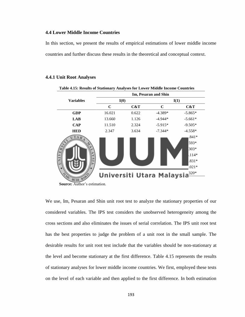
193
4.4 Lower Middle Income Countries
In this section, we present the results of empirical estimations of lower middle income
countries and further discuss these results in the theoretical and conceptual context.
4.4.1 Unit Root Analyses
Table 4.15: Results of Stationary Analyses for Lower Middle Income Countries
Variables
Im, Pesaran and Shin
I(0) I(1)
C C&T C C&T
GDP 16.021 0.622 -4.389* -5.865*
LAB 13.660 1.126 -4.944* -5.661*
CAP 11.510 2.324 -5.915* -9.505*
HED 2.347 3.634 -7.344* -4.558*
INF -0.213 -0.500 -25.372* -21.841*
DCF 1.370 -0.291 -11.744* -9.593*
GCE 12.965 4.197 -3.556* -7.303*
FDI 0.512 -0.947 -18.140* -14.114*
EXP -0.798 -0.604 -14.949* -11.831*
REM 8.708 2.164 -10.903* -10.021*
EXD 10.475 4.945 -6.408* -7.320*
*, **, *** indicates significance level respectively at 1%, 5% and 10%.
Source: Author‘s estimation.
We use, Im, Pesaran and Shin unit root test to analyze the stationary properties of our
considered variables. The IPS test considers the unobserved heterogeneity among the
cross sections and also eliminates the issues of serial correlation. The IPS unit root test
has the best properties to judge the problem of a unit root in the small sample. The
desirable results for unit root test include that the variables should be non-stationary at
the level and become stationary at the first difference. Table 4.15 represents the results
of stationary analyses for lower middle income countries. We first, employed these tests
on the level of each variable and then applied to the first difference. In both estimation

194
procedures of level and first difference, we also analyze the results in two dimensions,
i.e. with constant and with constant and trend. Results indicate that all the variables are
non-stationary at level and become stationary at first difference. These results confirm
that there is no problem of unit root in our variables of lower middle income countries
and we can further use these variables for the long run estimations.
4.4.2 Cointegration Analyses
After having the confirmation from unit root test that our variables have a stationary
properties of I(1) which is the requirement to perform panel cointegration techniques,
we applied two methods of panel cointegration i.e. Pedroni cointegration (1999) and
Kao cointegration (1999) to analyze the long run relationship among foreign capital
inflows, banking crisis, currency crisis and economic growth in lower middle income
countries. These tests are based on the two-step residual based cointegration tests of
Engle-Granger (1987). The Pedroni cointegration based on a seven statistical value. The
Pedroni cointegration is useful to control the biasness of country size and also solve the
issues of heterogeneity (Das & Choudhary, 2011). The Kao cointegration method
follows the same basic approached as used in the Pedroni cointegration, but also control
the issues of cross-section specific intercepts and homogenous coefficients.

195
Table 4.16: Results of Pedroni ((Engle-Granger based) Panel Cointegration in Lower Middle Income Countries
Estimates Stats. Prob.
GDP = f (LAB+CAP+HED+INF+DCF+GCE+BAC)
Panel v-statistic 3.455 0.000
Panel rho-statistic 5.565 1.000
Panel PP statistic -2.838 0.002
Panel ADF statistic -3.425 0.000
Alternative Hypothesis: Individual AR Coefficient
Group rho-statistic 7.089 1.000
Group PP statistic -6.512 0.000
Group ADF statistic -4.350 0.000
GDP = f (LAB+CAP+HED+INF+DCF+GCE+CRC)
Panel v-statistic 3.302 0.001
Panel rho-statistic 5.252 1.000
Panel PP statistic -0.423 0.336
Panel ADF statistic -1.650 0.050
Alternative Hypothesis: Individual AR Coefficient
Group rho-statistic 7.012 1.000
Group PP statistic -1.674 0.047
Group ADF statistic -2.100 0.018
GDP = f (LAB+CAP+HED+INF+DCF+GCE+FDI)
Panel v-statistic -0.057 0.523
Panel rho-statistic 5.758 1.000
Panel PP statistic -1.338 0.091
Panel ADF statistic -2.651 0.004
Alternative Hypothesis: Individual AR Coefficient
Group rho-statistic 7.289 1.000
Group PP statistic -4.528 0.000
Group ADF statistic -5.198 0.000
GDP = f (LAB+CAP+HED+INF+DCF+GCE+EXP)
Panel v-statistic 2.200 0.014
Panel rho-statistic 5.829 1.000
Panel PP statistic -1.958 0.025
Panel ADF statistic -3.524 0.000
Alternative Hypothesis: Individual AR Coefficient
Group rho-statistic 7.719 1.000
Group PP statistic -3.017 0.001
Group ADF statistic -3.515 0.000
GDP = f (LAB+CAP+HED+INF+DCF+GCE+REM)
Panel v-statistic 2.420 0.008
Panel rho-statistic 5.796 1.000
Panel PP statistic -2.239 0.013
Panel ADF statistic -2.580 0.005
Alternative Hypothesis: Individual AR Coefficient
Group rho-statistic 7.001 1.000
Group PP statistic -6.144 0.000
Group ADF statistic -4.364 0.000
GDP = f (LAB+CAP+HED+INF+DCF+GCE+EXD)
Panel v-statistic 2.382 0.009
Panel rho-statistic 5.491 1.000
Panel PP statistic -2.410 0.008
Panel ADF statistic -3.340 0.000
Alternative Hypothesis: Individual AR Coefficient
Group rho-statistic 7.239 1.000
Group PP statistic -6.449 0.000
Group ADF statistic -4.068 0.000
The null hypothesis of Pedroni's (1997) panel cointegration procedure is no cointegration
Source: Author‘s estimation.
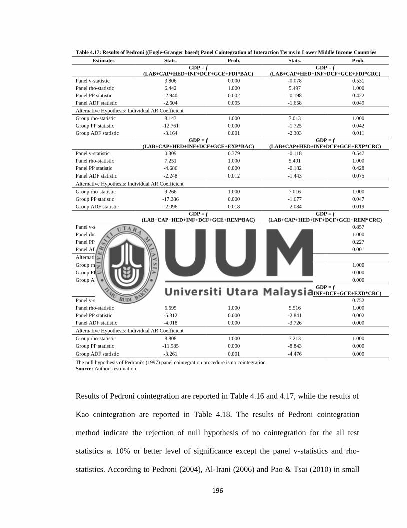
196
Table 4.17: Results of Pedroni ((Engle-Granger based) Panel Cointegration of Interaction Terms in Lower Middle Income Countries
Estimates Stats. Prob. Stats. Prob.
GDP = f
(LAB+CAP+HED+INF+DCF+GCE+FDI*BAC)
GDP = f
(LAB+CAP+HED+INF+DCF+GCE+FDI*CRC)
Panel v-statistic 3.806 0.000 -0.078 0.531
Panel rho-statistic 6.442 1.000 5.497 1.000
Panel PP statistic -2.940 0.002 -0.198 0.422
Panel ADF statistic -2.604 0.005 -1.658 0.049
Alternative Hypothesis: Individual AR Coefficient
Group rho-statistic 8.143 1.000 7.013 1.000
Group PP statistic -12.761 0.000 -1.725 0.042
Group ADF statistic -3.164 0.001 -2.303 0.011
GDP = f
(LAB+CAP+HED+INF+DCF+GCE+EXP*BAC)
GDP = f
(LAB+CAP+HED+INF+DCF+GCE+EXP*CRC)
Panel v-statistic 0.309 0.379 -0.118 0.547
Panel rho-statistic 7.251 1.000 5.491 1.000
Panel PP statistic -4.686 0.000 -0.182 0.428
Panel ADF statistic -2.248 0.012 -1.443 0.075
Alternative Hypothesis: Individual AR Coefficient
Group rho-statistic 9.266 1.000 7.016 1.000
Group PP statistic -17.286 0.000 -1.677 0.047
Group ADF statistic -2.096 0.018 -2.084 0.019
GDP = f
(LAB+CAP+HED+INF+DCF+GCE+REM*BAC)
GDP = f
(LAB+CAP+HED+INF+DCF+GCE+REM*CRC)
Panel v-statistic 2.698 0.004 -1.066 0.857
Panel rho-statistic 7.620 1.000 5.869 1.000
Panel PP statistic -1.894 0.029 -0.749 0.227
Panel ADF statistic -1.707 0.044 -3.215 0.001
Alternative Hypothesis: Individual AR Coefficient
Group rho-statistic 9.333 1.000 7.774 1.000
Group PP statistic -15.476 0.000 -3.704 0.000
Group ADF statistic -2.768 0.003 -3.744 0.000
GDP = f
(LAB+CAP+HED+INF+DCF+GCE+EXD*BAC)
GDP = f
(LAB+CAP+HED+INF+DCF+GCE+EXD*CRC)
Panel v-statistic 2.605 0.005 -0.680 0.752
Panel rho-statistic 6.695 1.000 5.516 1.000
Panel PP statistic -5.312 0.000 -2.841 0.002
Panel ADF statistic -4.018 0.000 -3.726 0.000
Alternative Hypothesis: Individual AR Coefficient
Group rho-statistic 8.808 1.000 7.213 1.000
Group PP statistic -11.985 0.000 -8.843 0.000
Group ADF statistic -3.261 0.001 -4.476 0.000
The null hypothesis of Pedroni's (1997) panel cointegration procedure is no cointegration
Source: Author's estimation.
Results of Pedroni cointegration are reported in Table 4.16 and 4.17, while the results of
Kao cointegration are reported in Table 4.18. The results of Pedroni cointegration
method indicate the rejection of null hypothesis of no cointegration for the all test
statistics at 10% or better level of significance except the panel v-statistics and rho-
statistics. According to Pedroni (2004), Al-Irani (2006) and Pao & Tsai (2010) in small

197
time dimensions, the panel v-statistics and rho-statistics may have a very low power.
Furthermore, Guterrez (2003) concludes that group statistics (especially Augmented
Dickey Fuller (ADF) and Phillips and Perron (PP) have the best power to judge the long
run cointegration among the test statistics of Pedroni (1999). Therefore, we can
conclude that the foreign capital inflows, banking crisis, currency crisis and economic
growth are cointegrated in the long run in the sample of lower middle income countries.
Results of Kao cointegration are reported in Table 4.18. The results of the Kao
cointegration method also indicate the rejection of the null hypothesis of no
cointegration in the favor of valid long run cointegration for the all test statistics at the 1
% level of significance in low income countries.
Table 4.18: Results of Kao (Engle-Granger based) Panel Cointegration in Lower Middle Income Countries
Estimates Stats. Prob.
GDP = f (LAB+CAP+HED+INF+DCF+GCE+BAC)
Panel ADF statistic -6.512 0.000
GDP = f (LAB+CAP+HED+INF+DCF+GCE+CRC)
Panel ADF statistic -5.959 0.000
GDP = f (LAB+CAP+HED+INF+DCF+GCE+FDI)
Panel ADF statistic -6.243 0.000
GDP = f (LAB+CAP+HED+INF+DCF+GCE+EXP)
Panel ADF statistic -5.915 0.000
GDP = f (LAB+CAP+HED+INF+DCF+GCE+REM)
Panel ADF statistic -5.556 0.000
GDP = f (LAB+CAP+HED+INF+DCF+GCE+EXD)
Panel ADF statistic -6.165 0.000
GDP = f (LAB+CAP+HED+INF+DCF+GCE+FDI*BAC)
Panel ADF statistic -6.579 0.000
GDP = f (LAB+CAP+HED+INF+DCF+GCE+FDI*CRC)
Panel ADF statistic -5.966 0.000
GDP = f (LAB+CAP+HED+INF+DCF+GCE+EXP*BAC)
Panel ADF statistic -6.505 0.000
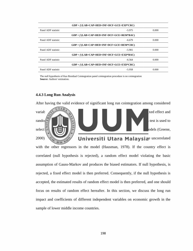
198
GDP = f (LAB+CAP+HED+INF+DCF+GCE+EXP*CRC)
Panel ADF statistic -5.975 0.000
GDP = f (LAB+CAP+HED+INF+DCF+GCE+REM*BAC)
Panel ADF statistic -6.679 0.000
GDP = f (LAB+CAP+HED+INF+DCF+GCE+REM*CRC)
Panel ADF statistic -5.901 0.000
GDP = f (LAB+CAP+HED+INF+DCF+GCE+EXD*BAC)
Panel ADF statistic -6.564 0.000
GDP = f (LAB+CAP+HED+INF+DCF+GCE+EXD*CRC)
Panel ADF statistic -5.958 0.000
The null hypothesis of Kao Residual Cointegration panel cointegration procedure is no cointegration
Source: Authors' estimation.
4.4.3 Long Run Analysis
After having the valid evidence of significant long run cointegration among considered
variables, the next step is to estimate the long run coefficients. We used fixed effect and
random effect methods to analyze the long run relationship. The Hausman test is used to
select the best preferable model between fixed effect and random effect models (Greene,
2000). The null hypothesis of Hausman test is that the country effects are uncorrelated
with the other regressors in the model (Hausman, 1978). If the country effect is
correlated (null hypothesis is rejected), a random effect model violating the basic
assumption of Gauss-Markov and produces the biased estimators. If null hypothesis, is
rejected, a fixed effect model is then preferred. Consequently, if the null hypothesis is
accepted, the estimated results of random effect model is then preferred, and one should
focus on results of random effect hereafter. In this section, we discuss the long run
impact and coefficients of different independent variables on economic growth in the
sample of lower middle income countries.

199
Banking Crisis and Currency Crisis
The results which explain the long run impact of banking crisis and currency crisis on
economic growth is presented in Table 4.19. The results of banking crisis are reported in
model I whereas, the results of currency crisis are reported in model II. Results of both
models indicate that the prob value of Hausman test is significant (0.001) and (0.001),
which confirm the rejection of null hypothesis and concluded that the fixed effect model
is preferred over random effect model. Furthermore, the statistical value of Variance
Inflation factor (VIF) also suggest that there is no issue of multicollinearity exist among
the independent variables of estimated models. Results also indicate the negative and
significant impact of the banking crisis on economic growth, whereas, the positive and
significant influence of currency crisis on economic growth is observed. It is concluded
that the banking crises decrease the progress of the economic development, whereas,
currency crisis helps to promote economic growth in lower middle income countries.
Table 4.19: Long Run Results of Banking and Currency Crisis in Lower Middle Income Countries
Variables
I II
FE RE FE RE
Coeff. Prob. VIF Coeff. Prob. VIF Coeff. Prob. VIF Coeff. Prob. VIF
α 21.352 0.000
20.129 0.000
21.537 0.000
20.306 0.000
LAB 0.025 0.592 1.342 0.008 0.859 1.349 0.019 0.677 1.343 0.029 0.515 1.344
CAP 0.147 0.000 2.301 0.149 0.000 2.411 0.150 0.000 2.275 0.155 0.000 2.412
HED 0.073 0.000 1.241 0.083 0.000 1.314 0.075 0.000 1.239 0.078 0.000 1.286
INF 0.000 0.027 1.087 0.000 0.019 1.087 0.000 0.107 1.151 0.000 0.148 1.149
DCF 0.053 0.000 1.298 0.063 0.000 1.294 0.040 0.000 1.238 0.047 0.000 1.253
GCE 0.039 0.023 2.199 0.053 0.002 2.377 0.041 0.017 2.232 0.047 0.006 2.386
BAC -0.037 0.002 1.079 -0.044 0.000 1.072
CRC -0.025 0.004 1.097 -0.025 0.003 1.097
Adj. R2 0.998 0.587 0.998 0.568
Hausman Stats.
(Prob) 24.453 (0.001) 24.468 (0.001)
F-stats (Prob.) 26118.05 (0.000) 91.891 (0.000) 25910.36 (0.000) 80.496 (0.000)
Source: Author's estimation.

200
Furthermore, the results of control variables show that the labor force, capital formation,
higher education development, domestic credit by financial sector, inflation and
government consumption expenditure have significant positive impact on economic
growth.
Foreign Direct Investment
The results which explain the long run impact of foreign direct investment and
interaction terms of banking and currency crisis with foreign direct investment on
economic growth is presented in Table 4.20. Model I, II and III show the results of
foreign direct investment, interaction of foreign direct investment and banking crisis and
interaction of foreign direct investment and currency crisis respectively. Results of all
three models indicate that the prob value of Hausman test is significant (0.001), (0.001)
and (0.001), which confirm the acceptance of null hypothesis and concluded that the
fixed effect model is preferred over random effect model. Results indicate the positive
and significant impact of foreign direct investment on economic growth. The coefficient
of foreign direct investment is showing that the 1% increase in FDI causes the increase
in economic growth by 0.007%. This finding is consistent with the previous empirical
studies. Results of model II confirm that the impact of foreign direct investment on
economic growth becomes negative and significant in the presence of systemic banking
crises. Results of model III confirm that the impact of foreign direct investment on
economic growth remains positive and significant in the presence of currency crises.
However, the magnitude of the relationship is dragged down from 0.007 to 0.001.
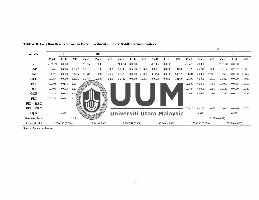
201
Table 4.20: Long Run Results of Foreign Direct Investment in Lower Middle Income Countries
Variables
I II III
FE RE FE RE FE RE
Coeff. Prob. VIF Coeff. Prob. VIF Coeff. Prob. VIF Coeff. Prob. VIF Coeff. Prob. VIF Coeff. Prob. VIF
α 21.7809 0.0000
20.5152 0.0000
21.4654 0.0000
20.1062 0.0000
21.5211 0.0000
20.2531 0.0000
LAB 0.0440 0.3364 1.3547 0.0193 0.6706 1.3408 0.0296 0.5210 1.3376 0.0081 0.8520 1.3493 0.0323 0.4748 1.3543 0.0167 0.7032 1.3555
CAP 0.1523 0.0000 2.1716 0.1546 0.0000 2.4682 0.1470 0.0000 2.3006 0.1494 0.0000 2.4052 0.1494 0.0000 2.2183 0.1530 0.0000 2.3652
HED 0.0767 0.0000 1.2776 0.0774 0.0000 1.2855 0.0742 0.0000 1.2389 0.0823 0.0000 1.3140 0.0795 0.0000 1.2603 0.0823 0.0000 1.3088
INF 0.0004 0.0114 1.1022 0.0004 0.0213 1.1065 0.0004 0.0212 1.0882 0.0004 0.0192 1.0874 0.0003 0.0472 1.1379 0.0003 0.0685 1.1365
DCF 0.0406 0.0003 1.2707 0.0485 0.0000 1.2563 0.0520 0.0000 1.3099 0.0632 0.0000 1.2972 0.0434 0.0000 1.2179 0.0510 0.0000 1.2336
GCE 0.0419 0.0174 2.1449 0.0386 0.0231 2.3526 0.0383 0.0240 2.2020 0.0531 0.0015 2.3754 0.0460 0.0073 2.2116 0.0531 0.0017 2.3781
FDI 0.0071 0.0591 1.0703 0.0040 0.2678 1.2049
FDI * BAC
-0.0020 0.0010 1.0862 -0.0023 0.0002 1.0737
FDI * CRC 0.0010 0.0182 1.0772 0.0010 0.0146 1.0766
Adj. R2 0.998 0.560 0.998 0.588 0.998 0.577
Hausman. Stats. 24.557 (0.001) 24.460 (0.001) 24.899 (0.001)
F-stats (Prob.) 22380.02 (0.000) 78.041 (0.000) 26067.41 (0.000) 92.243 (0.000) 25306.33 (0.000) 87.963 (0.000)
Source: Author's estimation.
202
These findings conclude that the banking and currency crisis are harmful for the
relationship of foreign direct investment and economic growth in lower middle income
countries.
Furthermore, the results of control variables show that the labor force, capital formation,
higher education development, domestic credit by financial sector, inflation and
government consumption expenditure have significant positive impact on economic
growth.
Export of Goods and Services
The results which explain the long run impact of exports of goods and services and
interaction terms of banking and currency crisis with exports of goods and services on
economic growth is presented in Table 4.21. Model I, II and III show the results of
exports of goods and services, interaction of exports and banking crisis and interaction
of exports and currency crisis respectively. Results of all three models indicate that the
prob value of Hausman test is significant (0.002), (0.001) and (0.001), which confirm
the acceptance of null hypothesis and concluded that the fixed effect model is preferred
over random effect model. Furthermore, the statistical value of Variance Inflation factor
(VIF) also suggest that there is no issue of multicollinearity exist among the independent
variables of estimated models. Results indicate the positive and significant impact of
exports of goods and services on economic growth. The coefficient of exports of goods
and services is showing that the 1% increase in exports causes the increase in economic
growth by 0.104%. This finding is consistent with the previous empirical studies.
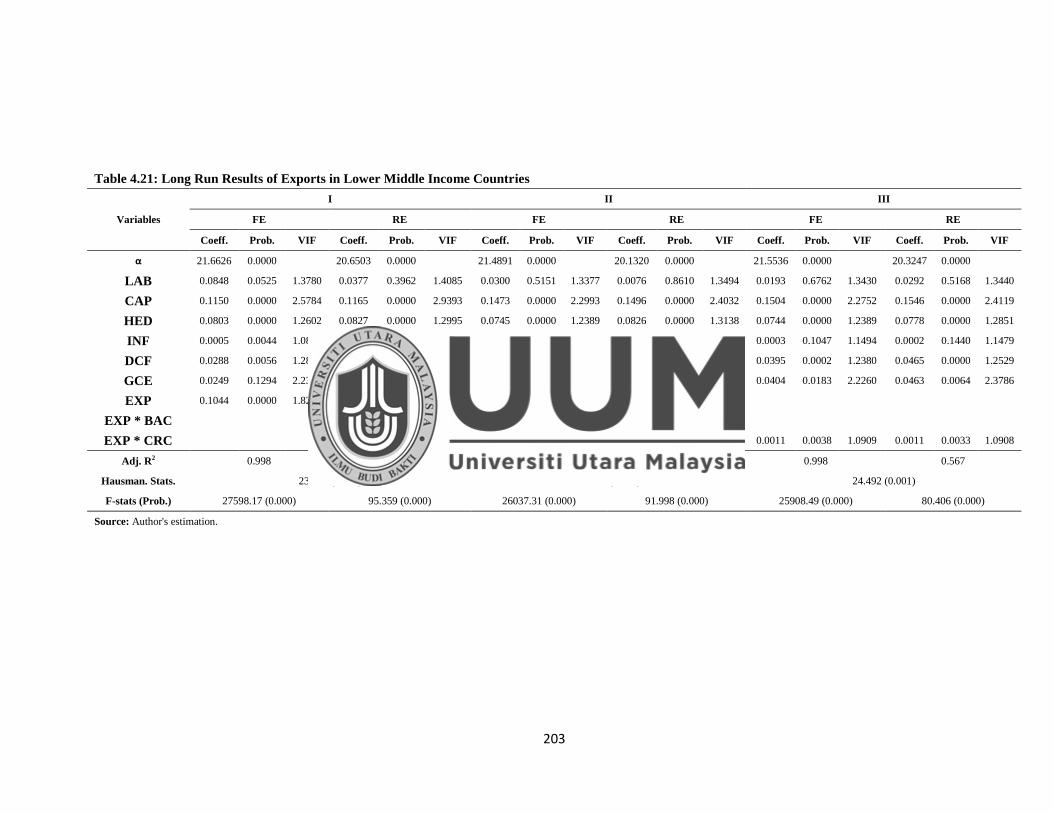
203
Table 4.21: Long Run Results of Exports in Lower Middle Income Countries
Variables
I II III
FE RE FE RE FE RE
Coeff. Prob. VIF Coeff. Prob. VIF Coeff. Prob. VIF Coeff. Prob. VIF Coeff. Prob. VIF Coeff. Prob. VIF
α 21.6626 0.0000
20.6503 0.0000
21.4891 0.0000
20.1320 0.0000
21.5536 0.0000
20.3247 0.0000
LAB 0.0848 0.0525 1.3780 0.0377 0.3962 1.4085 0.0300 0.5151 1.3377 0.0076 0.8610 1.3494 0.0193 0.6762 1.3430 0.0292 0.5168 1.3440
CAP 0.1150 0.0000 2.5784 0.1165 0.0000 2.9393 0.1473 0.0000 2.2993 0.1496 0.0000 2.4032 0.1504 0.0000 2.2752 0.1546 0.0000 2.4119
HED 0.0803 0.0000 1.2602 0.0827 0.0000 1.2995 0.0745 0.0000 1.2389 0.0826 0.0000 1.3138 0.0744 0.0000 1.2389 0.0778 0.0000 1.2851
INF 0.0005 0.0044 1.0893 0.0004 0.0116 1.0887 0.0004 0.0219 1.0884 0.0004 0.0200 1.0875 0.0003 0.1047 1.1494 0.0002 0.1440 1.1479
DCF 0.0288 0.0056 1.2870 0.0340 0.0011 1.3211 0.0515 0.0000 1.3038 0.0627 0.0000 1.2919 0.0395 0.0002 1.2380 0.0465 0.0000 1.2529
GCE 0.0249 0.1294 2.2315 0.0254 0.1195 2.4341 0.0379 0.0254 2.2004 0.0527 0.0017 2.3733 0.0404 0.0183 2.2260 0.0463 0.0064 2.3786
EXP 0.1044 0.0000 1.8277 0.1060 0.0000 2.0647
EXP * BAC
-0.0017 0.0013 1.0805 -0.0019 0.0003 1.0690
EXP * CRC 0.0011 0.0038 1.0909 0.0011 0.0033 1.0908
Adj. R2 0.998 0.609 0.998 0.587 0.998 0.567
Hausman. Stats. 23.289 (0.002) 24.478 (0.001) 24.492 (0.001)
F-stats (Prob.) 27598.17 (0.000) 95.359 (0.000) 26037.31 (0.000) 91.998 (0.000) 25908.49 (0.000) 80.406 (0.000)
Source: Author's estimation.
204
Results of model II confirm that the impact of exports on economic growth becomes
significantly negative in the presence of systemic banking crises. Results of model III
confirm that the impact of export on economic growth remains positive and significant
in the presence of currency crises. However, the magnitude of the relationship is
dragged down from 0.104 to 0.001. These findings conclude that the banking and
currency crisis are harmful for the relationship of export and economic growth in lower
middle income countries.
Furthermore, the results of control variables show that the labor force, capital formation,
higher education development, domestic credit by financial sector, inflation and
government consumption expenditure have significant positive impact on economic
growth.
Workers’ Remittances
The results which explain the long run impact of workers‘ remittances and interaction
terms of banking and currency crisis with workers‘ remittances on economic growth is
presented in Table 4.22. Model I, II and III show the results of workers‘ remittances,
interaction of workers‘ remittances and banking crisis and interaction of workers‘
remittances and currency crisis respectively. Results of all three models indicate that the
prob value of Hausman test is significant (0.002), (0.002) and (0.001), which confirm
the acceptance of null hypothesis and concluded that the fixed effect model is preferred
over random effect model. Furthermore, the statistical value of Variance Inflation factor
(VIF) also suggest that there is no issue of multicollinearity exist among the independent

205
variables of estimated models. Results indicate the positive and significant impact of
workers‘ remittances on economic growth. This finding is consistent with the previous
empirical studies. The coefficient of workers‘ remittances is showing that the 1%
increase in remittances causes the increase in economic growth by 0.013%. Results of
model II confirm that the impact of workers‘ remittances on economic growth becomes
significantly negative in the presence of systemic banking crises. Results of model III
confirm that the impact of remittances on economic growth remains positive and
significant in the presence of currency crises. However, the magnitude of the
relationship is dragged down from 0.013 to 0.001. These findings conclude that the
banking and currency crisis are harmful for the relationship of workers‘ remittances and
economic growth in lower middle income countries.
Furthermore, the results of control variables show that the labor force, capital formation,
higher education development, domestic credit by financial sector, inflation and
government consumption expenditure have significant positive impact on economic
growth.
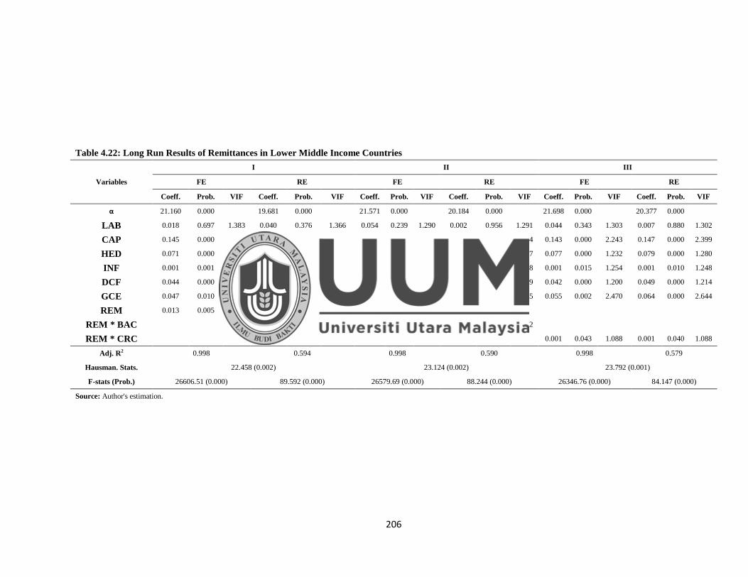
206
Table 4.22: Long Run Results of Remittances in Lower Middle Income Countries
Variables
I II III
FE RE FE RE FE RE
Coeff. Prob. VIF Coeff. Prob. VIF Coeff. Prob. VIF Coeff. Prob. VIF Coeff. Prob. VIF Coeff. Prob. VIF
α 21.160 0.000
19.681 0.000
21.571 0.000
20.184 0.000
21.698 0.000
20.377 0.000
LAB 0.018 0.697 1.383 0.040 0.376 1.366 0.054 0.239 1.290 0.002 0.956 1.291 0.044 0.343 1.303 0.007 0.880 1.302
CAP 0.145 0.000 2.233 0.148 0.000 2.420 0.142 0.000 2.253 0.144 0.000 2.434 0.143 0.000 2.243 0.147 0.000 2.399
HED 0.071 0.000 1.254 0.073 0.000 1.316 0.078 0.000 1.233 0.081 0.000 1.287 0.077 0.000 1.232 0.079 0.000 1.280
INF 0.001 0.001 1.225 0.001 0.000 1.215 0.001 0.002 1.206 0.001 0.001 1.198 0.001 0.015 1.254 0.001 0.010 1.248
DCF 0.044 0.000 1.189 0.052 0.000 1.206 0.051 0.000 1.259 0.060 0.000 1.269 0.042 0.000 1.200 0.049 0.000 1.214
GCE 0.047 0.010 2.488 0.055 0.002 2.714 0.058 0.001 2.481 0.068 0.000 2.675 0.055 0.002 2.470 0.064 0.000 2.644
REM 0.013 0.005 1.205 0.015 0.001 1.218
REM * BAC
-0.002 0.006 1.080 -0.002 0.001 1.072
REM * CRC 0.001 0.043 1.088 0.001 0.040 1.088
Adj. R2 0.998 0.594 0.998 0.590 0.998 0.579
Hausman. Stats. 22.458 (0.002) 23.124 (0.002) 23.792 (0.001)
F-stats (Prob.) 26606.51 (0.000) 89.592 (0.000) 26579.69 (0.000) 88.244 (0.000) 26346.76 (0.000) 84.147 (0.000)
Source: Author's estimation.
207
External Debt
The results which explain the long run impact of external debt and interaction terms of
banking and currency crisis with external debt on economic growth is presented in Table
4.23. Model I, II and III show the results of external debt, interaction of external debt
and banking crisis and interaction of external debt and currency crisis respectively.
Results of all three models indicate that the prob value of Hausman test is significant
(0.000), (0.001) and (0.001), which confirm the acceptance of null hypothesis and
concluded that the fixed effect model is preferred over random effect model.
Furthermore, the statistical value of Variance Inflation factor (VIF) also suggest that
there is no issue of multicollinearity exist among the independent variables of estimated
models. Results indicate the negative and significant impact of external debt on
economic growth. This finding is consistent with the previous empirical studies. The
coefficient of external debt is showing that the 1% increase in external debt causes the
decrease in economic growth by -0.047%. Results of model II confirm that the impact of
external debt on economic growth becomes significantly positive in the presence of
systemic banking crises. Results of model III confirm that the impact of external debt on
economic growth remain negative and significant in the presence of currency crises.
However, the magnitude of the relationship is dragged down from 0.047 to 0.004. These
findings conclude that the relationship of external debt and economic growth is getting
stronger in the period of banking and currency crisis in lower middle income countries.

208
Table 4.23: Long Run Results of External Debt in Lower Middle Income Countries
Variables
I II III
FE RE FE RE FE RE
Coeff. Prob. VIF Coeff. Prob. VIF Coeff. Prob. VIF Coeff. Prob. VIF Coeff. Prob. VIF Coeff. Prob. VIF
α 23.6010 0.0000
22.2560 0.0000
21.5747 0.0000
20.2969 0.0000
21.6284 0.0000
20.4041 0.0000
LAB 0.1554 0.0034 1.8063 0.0947 0.0643 1.7635 0.0270 0.5623 1.3377 0.0229 0.6128 1.3393 0.0204 0.6606 1.3426 0.0279 0.5372 1.3442
CAP 0.1398 0.0000 2.3511 0.1452 0.0000 2.4318 0.1509 0.0000 2.2813 0.1549 0.0000 2.4283 0.1505 0.0000 2.2758 0.1548 0.0000 2.4083
HED 0.0802 0.0000 1.2480 0.0819 0.0000 1.2807 0.0748 0.0000 1.2398 0.0784 0.0000 1.2885 0.0730 0.0000 1.2398 0.0763 0.0000 1.2847
INF 0.0003 0.0415 1.0940 0.0003 0.0512 1.0936 0.0004 0.0161 1.0899 0.0004 0.0235 1.0891 0.0003 0.0655 1.1239 0.0003 0.0894 1.1227
DCF 0.0556 0.0000 1.3075 0.0601 0.0000 1.3240 0.0470 0.0000 1.2871 0.0548 0.0000 1.2996 0.0400 0.0002 1.2364 0.0470 0.0000 1.2501
GCE 0.0238 0.1555 2.2256 0.0301 0.0703 2.3169 0.0342 0.0453 2.1892 0.0402 0.0174 2.3489 0.0374 0.0283 2.2015 0.0431 0.0107 2.3494
EXD 0.0468 0.0000 1.6390 -0.0406 0.0000 1.5931
EXD * BAC
0.0034 0.0835 1.0537 0.0040 0.0404 1.0516
EXD * CRC -0.0044 0.0084 1.0522 -0.0043 0.0094 1.0520
Adj. R2 0.998 0.564 0.998 0.565 0.998 0.565
Hausman. Stats. 26.817 (0.000) 24.387 (0.001) 24.606 (0.001)
F-stats (Prob.) 26821.77 (0.000) 79.154 (0.000) 25552.47 (0.000) 79.606 (0.000) 25813.81 (0.000) 79.445 (0.000)
Source: Author's estimation.

209
Furthermore, the results of control variables show that the labor force, capital formation,
higher education development, domestic credit by financial sector, inflation and
government consumption expenditure have significant positive impact on economic
growth.
4.5 Upper Middle Income Countries
In this section, we present the results of empirical estimations of upper middle income
countries and further discuss these results in the theoretical and conceptual context.
4.5.1 Unit Root Analyses
Table 4.24: Results of Stationary Analyses for Upper Middle Income Countries
Variables
Im, Pesaran and Shin
I(0) I(1)
C C&T C C&T
GDP 12.463 1.768 -9.398* -9.388*
LAB 6.433 0.625 -7.995* -9.033*
CAP 8.515 1.874 -8.744* -9.471*
HED -0.354 0.244 -12.67* -12.824*
INF 1.818 -0.158 -13.967* -11.510*
DCF 13.079 2.143 -8.907* -8.307*
GCE 6.479 -0.028 -10.229* -11.096*
FDI -0.973 -0.954 -20.082* -14.999*
EXP 1.985 -0.371 -16.009* -12.485*
REM 3.783 -0.358 -11.945* -8.847*
EXD 14.125 6.810 -6.086* -9.831*
*, **, *** indicates significance level respectively at 1%, 5% and 10%.
Source: Author‘s estimation.
We use, Im, Pesaran and Shin unit root test to analyze the stationary properties of our
considered variables. The IPS test considers the unobserved heterogeneity among the
cross sections and also eliminates the issues of serial correlation. The IPS unit root test
210
has the best properties to judge the problem of a unit root in the small sample. The
desirable results for the unit root test include that the variables should be non-stationary
at the level and become stationary at the first difference. Table 4.24 represents the
results of stationary analyses for upper middle income countries. We first, employed
these tests on level of each variables and then applied on the first difference. In both
estimation procedures of level and first difference, we also analyze the results in two
dimensions, i.e. with constant and with constant and trend. Results indicate that all the
variables are non-stationary at level and become stationary at first difference. These
results confirm that there is no problem of unit root in our variables of upper middle
income countries and we can further use these variables for the long run estimations.
4.5.2 Cointegration Analyses
After having the confirmation from unit root test that our variables have a stationary
properties of I(1) which is the requirement to perform panel cointegration techniques,
we applied two methods of panel cointegration i.e. Pedroni cointegration (1999) and
Kao cointegration (1999) to analyze the long run relationship among foreign capital
inflows, banking crisis, currency crisis and economic growth in upper middle income
countries. These tests are based on the two-step residual based cointegration tests of
Engle-Granger (1987). The Pedroni cointegration based on a seven statistic values. The
Pedroni cointegration is useful to control the biasness of country size and also solve the
issues of heterogeneity (Das & Choudhary, 2011). The Kao cointegration method
follows the same basic approached as used in the Pedroni cointegration, but also control
the issues of cross-section specific intercepts and homogenous coefficients.
Table 4.25: Results of Pedroni ((Engle-Granger based) Panel Cointegration in Upper Middle Income Countries

211
Estimates Stats. Prob.
GDP = f (LAB+CAP+HED+INF+DCF+GCE+BAC)
Panel v-statistic 0.894 0.186
Panel rho-statistic 5.860 1.000
Panel PP statistic -0.116 0.454
Panel ADF statistic -1.291 0.098
Alternative Hypothesis: Individual AR Coefficient
Group rho-statistic 7.529 1.000
Group PP statistic -8.764 0.000
Group ADF statistic -3.917 0.000
GDP = f (LAB+CAP+HED+INF+DCF+GCE+CRC)
Panel v-statistic -0.101 0.540
Panel rho-statistic 5.909 1.000
Panel PP statistic -1.869 0.031
Panel ADF statistic -2.643 0.004
Alternative Hypothesis: Individual AR Coefficient
Group rho-statistic 7.431 1.000
Group PP statistic -9.451 0.000
Group ADF statistic -5.200 0.000
GDP = f (LAB+CAP+HED+INF+DCF+GCE+FDI)
Panel v-statistic -2.209 0.986
Panel rho-statistic 6.443 1.000
Panel PP statistic -7.796 0.000
Panel ADF statistic -4.379 0.000
Alternative Hypothesis: Individual AR Coefficient
Group rho-statistic 8.679 1.000
Group PP statistic -14.144 0.000
Group ADF statistic -7.030 0.000
GDP = f (LAB+CAP+HED+INF+DCF+GCE+EXP)
Panel v-statistic -3.890 1.000
Panel rho-statistic 7.020 1.000
Panel PP statistic -5.794 0.000
Panel ADF statistic -3.403 0.000
Alternative Hypothesis: Individual AR Coefficient
Group rho-statistic 8.548 1.000
Group PP statistic -14.773 0.000
Group ADF statistic -4.525 0.000
GDP = f (LAB+CAP+HED+INF+DCF+GCE+REM)
Panel v-statistic 2.726 0.003
Panel rho-statistic 5.845 1.000
Panel PP statistic -8.245 0.000
Panel ADF statistic -7.441 0.000
Alternative Hypothesis: Individual AR Coefficient
Group rho-statistic 8.278 1.000
Group PP statistic -18.709 0.000
Group ADF statistic -8.761 0.000
GDP = f (LAB+CAP+HED+INF+DCF+GCE+EXD)
Panel v-statistic -1.952 0.975
Panel rho-statistic 5.945 1.000
Panel PP statistic -8.819 0.000
Panel ADF statistic -3.930 0.000
Alternative Hypothesis: Individual AR Coefficient
Group rho-statistic 8.278 1.000
Group PP statistic -18.021 0.000
Group ADF statistic -6.721 0.000
The null hypothesis of Pedroni's (1997) panel cointegration procedure is no cointegration Source: Author's estimation.

212
Table 4.26: Results of Pedroni ((Engle-Granger based) Panel Cointegration of Interaction Terms in Upper Middle Income Countries
Estimates Stats. Prob. Stats. Prob.
GDP = f
(LAB+CAP+HED+INF+DCF+GCE+FDI*BAC)
GDP = f
(LAB+CAP+HED+INF+DCF+GCE+FDI*CRC)
Panel v-statistic -4.812 1.000
0.115 0.454
Panel rho-statistic 2.927 0.998
5.856 1.000
Panel PP statistic -2.863 0.002
-1.805 0.036
Panel ADF statistic -4.227 0.000
-2.228 0.013
Alternative Hypothesis: Individual AR Coefficient
Group rho-statistic 5.587 1.000
7.422 1.000
Group PP statistic -0.819 0.206
-9.315 0.000
Group ADF statistic -3.183 0.001
-4.227 0.000
GDP = f
(LAB+CAP+HED+INF+DCF+GCE+EXP*BAC)
GDP = f
(LAB+CAP+HED+INF+DCF+GCE+EXP*CRC)
Panel v-statistic -4.822 1.000
-5.003 1.000
Panel rho-statistic 2.962 0.999
3.320 1.000
Panel PP statistic -2.774 0.003
-2.075 0.019
Panel ADF statistic -4.290 0.000
-2.714 0.003
Alternative Hypothesis: Individual AR Coefficient
Group rho-statistic 7.525 1.000
5.374 1.000
Group PP statistic -8.794 0.000
-3.862 0.000
Group ADF statistic -3.915 0.000
-3.294 0.001
GDP = f
(LAB+CAP+HED+INF+DCF+GCE+REM*BAC)
GDP = f
(LAB+CAP+HED+INF+DCF+GCE+REM*CRC)
Panel v-statistic -4.824 1.000
-0.097 0.539
Panel rho-statistic 2.941 0.998
5.908 1.000
Panel PP statistic -2.770 0.003
-1.835 0.033
Panel ADF statistic -4.262 0.000
-2.262 0.012
Alternative Hypothesis: Individual AR Coefficient
Group rho-statistic 5.577 1.000
7.427 1.000
Group PP statistic -0.704 0.241
-9.434 0.000
Group ADF statistic -3.283 0.001
-4.301 0.000
GDP = f
(LAB+CAP+HED+INF+DCF+GCE+EXD*BAC)
GDP = f
(LAB+CAP+HED+INF+DCF+GCE+EXD*CRC)
Panel v-statistic -4.824 1.000
-0.088 0.535
Panel rho-statistic 2.967 0.999
5.902 1.000
Panel PP statistic -2.750 0.003
-1.886 0.030
Panel ADF statistic -4.274 0.000
-2.655 0.004
Alternative Hypothesis: Individual AR Coefficient
Group rho-statistic 5.627 1.000
7.423 1.000
Group PP statistic -0.747 0.227
-9.458 0.000
Group ADF statistic -3.249 0.001 -5.183 0.000
The null hypothesis of Pedroni's (1997) panel cointegration procedure is no cointegration
Source: Author's estimation.
Results of Pedroni cointegration are reported in Table 4.25 and 4.26, while the results of
Kao cointegration are reported in Table 4.27. The results of Pedroni cointegration
method indicate the rejection of null hypothesis of no cointegration for the all test
statistics at 10% or better level of significance except the panel v-statistics and rho-
statistics. According to Pedroni (2004), Al-Irani (2006) and Pao & Tsai (2010) in small

213
time dimensions, the panel v-statistics and rho-statistics may have a very low power.
Furthermore, Guterrez (2003) concludes that group statistics (especially Augmented
Dickey Fuller (ADF) and Phillips and Perron (PP) have the best power to judge the long
run cointegration among the test statistics of Pedroni (1999). Therefore, we can
conclude that the foreign capital inflows, banking crisis, currency crisis and economic
growth are cointegrated in the long run in the sample of upper middle income countries.
Results of Kao cointegration are reported in Table 4.27. The results of the Kao
cointegration method also indicate the rejection of the null hypothesis of no
cointegration in the favor of valid long run cointegration for the all test statistics at the 1
% level of significance in low income countries.
Table 4.27: Results of Kao (Engle-Granger based) Panel Cointegration in Upper Middle Income Countries
Estimates Stats. Prob.
GDP = f (LAB+CAP+HED+INF+DCF+GCE+BAC)
Panel ADF statistic -5.910 0.000
GDP = f (LAB+CAP+HED+INF+DCF+GCE+CRC)
Panel ADF statistic -6.358 0.000
GDP = f (LAB+CAP+HED+INF+DCF+GCE+FDI)
Panel ADF statistic -5.703 0.000
GDP = f (LAB+CAP+HED+INF+DCF+GCE+EXP)
Panel ADF statistic -4.329 0.000
GDP = f (LAB+CAP+HED+INF+DCF+GCE+REM)
Panel ADF statistic -5.815 0.000
GDP = f (LAB+CAP+HED+INF+DCF+GCE+EXD)
Panel ADF statistic -5.673 0.000
GDP = f (LAB+CAP+HED+INF+DCF+GCE+FDI*BAC)
Panel ADF statistic -5.706 0.000
GDP = f (LAB+CAP+HED+INF+DCF+GCE+FDI*CRC)
Panel ADF statistic -6.434 0.000
GDP = f (LAB+CAP+HED+INF+DCF+GCE+EXP*BAC)
Panel ADF statistic -5.717 0.000

214
GDP = f (LAB+CAP+HED+INF+DCF+GCE+EXP*CRC)
Panel ADF statistic -6.473 0.000
GDP = f (LAB+CAP+HED+INF+DCF+GCE+REM*BAC)
Panel ADF statistic -5.729 0.000
GDP = f (LAB+CAP+HED+INF+DCF+GCE+REM*CRC)
Panel ADF statistic -6.453 0.000
GDP = f (LAB+CAP+HED+INF+DCF+GCE+EXD*BAC)
Panel ADF statistic -5.733 0.000
GDP = f (LAB+CAP+HED+INF+DCF+GCE+EXD*CRC)
Panel ADF statistic -6.496 0.000
The null hypothesis of Kao Residual Cointegration panel cointegration procedure is no cointegration
Source: Authors' estimation.
4.5.3 Long Run Analysis
After having the valid evidence of significant long run cointegration among considered
variables, the next step is to estimate the long run coefficients. We used fixed effect and
random effect methods to analyze the long run relationship. The Hausman test is used to
select the best preferable model between fixed effect and random effect models (Greene,
2000). The null hypothesis of Hausman test is that the country effects are uncorrelated
with the other regressors in the model (Hausman, 1978). If the country effect is
correlated (null hypothesis is rejected), a random effect model violating the basic
assumption of Gauss-Markov and produces the biased estimators. If null hypothesis, is
rejected, a fixed effect model is then preferred. Consequently, if the null hypothesis is
accepted, the estimated results of random effect model is then preferred, and one should
focus on results of random effect hereafter. In this section, we discuss the long run
impact and coefficients of different independent variables on economic growth in the
sample of low income countries.
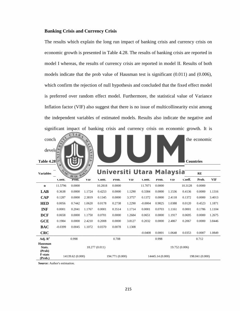
215
Banking Crisis and Currency Crisis
The results which explain the long run impact of banking crisis and currency crisis on
economic growth is presented in Table 4.28. The results of banking crisis are reported in
model I whereas, the results of currency crisis are reported in model II. Results of both
models indicate that the prob value of Hausman test is significant (0.011) and (0.006),
which confirm the rejection of null hypothesis and concluded that the fixed effect model
is preferred over random effect model. Furthermore, the statistical value of Variance
Inflation factor (VIF) also suggest that there is no issue of multicollinearity exist among
the independent variables of estimated models. Results also indicate the negative and
significant impact of banking crisis and currency crisis on economic growth. It is
concluded that the banking and currency crises decrease the progress of the economic
development in upper middle income countries.
Table 4.28: Long Run Results of Banking and Currency Crisis in Upper Middle Income Countries
Variables
I II
FE RE FE RE
Coeff. Prob. VIF Coeff. Prob. VIF Coeff. Prob. VIF Coeff. Prob. VIF
α 11.5796 0.0000
10.2818 0.0000
11.7071 0.0000
10.3128 0.0000
LAB 0.3638 0.0000 1.1724 0.4253 0.0000 1.1290 0.3384 0.0000 1.1536 0.4136 0.0000 1.1316
CAP 0.1287 0.0000 2.3819 0.1345 0.0000 3.3757 0.1372 0.0000 2.4118 0.1372 0.0000 3.4013
HED 0.0056 0.7442 1.0620 0.0178 0.2738 1.2290 -0.0004 0.9825 1.0388 0.0120 0.4523 1.1871
INF 0.0001 0.2041 1.1767 0.0001 0.3514 1.1714 0.0001 0.0703 1.1161 0.0001 0.1786 1.1104
DCF 0.0658 0.0000 1.1750 0.0701 0.0000 1.2684 0.0651 0.0000 1.1917 0.0695 0.0000 1.2675
GCE 0.1984 0.0000 2.4210 0.2008 0.0000 3.8127 0.2032 0.0000 2.4867 0.2067 0.0000 3.8446
BAC -0.0399 0.0045 1.1072 0.0370 0.0078 1.1308
CRC -0.0408 0.0001 1.0648 0.0353 0.0007 1.0849
Adj. R2 0.998 0.708 0.998 0.712
Hausman
Stats.
(Prob)
18.277 (0.011) 19.752 (0.006)
F-stats
(Prob.) 14139.62 (0.000) 194.771 (0.000) 14445.14 (0.000) 198.041 (0.000)
Source: Author's estimation.
216
Furthermore, the results of control variables show that the labor force, capital formation,
higher education development, domestic credit by financial sector, inflation and
government consumption expenditure have significant positive impact on economic
growth in upper middle income countries.
Foreign Direct Investment
The results which explain the long run impact of foreign direct investment and
interaction terms of banking and currency crisis with foreign direct investment on
economic growth is presented in Table 4.29. Model I, II and III show the results of foreign
direct investment, interaction of foreign direct investment and banking crisis and interaction of
foreign direct investment and currency crisis respectively. Results of all three models
indicate that the prob value of Hausman test is significant (0.008), (0.010) and (0.006),
which confirm the acceptance of null hypothesis and concluded that the fixed effect
model is preferred over random effect model. Furthermore, the statistical value of
Variance Inflation factor (VIF) also suggest that there is no issue of multicollinearity
exist among the independent variables of estimated models. Results indicate the positive
and significant impact of foreign direct investment on economic growth. The coefficient
of foreign direct investment is showing that the 1% increase in FDI causes the increase in
economic growth by 0.011%. This finding is consistent with the previous empirical studies.
Results of model II and III confirm that the impact of FDI on economic growth remains
positive and significant in the presence of banking and currency crises. However, the
magnitude of the relationship is dragged down from 0.011 to 0.002. These findings
conclude that the banking and currency crisis are harmful for the relationship of FDI and
economic growth in upper middle income countries.

217
Table 4.29: Long Run Results of Foreign Direct Investment in Upper Middle Income Countries
Variables
I II III
FE RE FE RE FE RE
Coeff. Prob. VIF Coeff. Prob. VIF Coeff. Prob. VIF Coeff. Prob. VIF Coeff. Prob. VIF Coeff. Prob. VIF
α 11.3392 0.0000
10.1961 0.0000
11.5777 0.0000
10.2813 0.0000
11.4731 0.0000
10.2834 0.0000
LAB 0.3738 0.0000 1.1832 0.4310 0.0000 1.1622 0.3638 0.0000 1.1724 0.4253 0.0000 1.1304 0.3578 0.0000 1.1732 0.4162 0.0000 1.1324
CAP 0.1183 0.0000 2.5241 0.1214 0.0000 3.9695 0.1285 0.0000 2.3819 0.1343 0.0000 3.3897 0.1311 0.0000 2.3896 0.1364 0.0000 3.4158
HED 0.0001 0.0402 1.1105 0.0001 0.1087 1.1040 0.0001 0.1565 1.1621 0.0001 0.2847 1.1564 0.0001 0.0828 1.1165 0.0001 0.1784 1.1103
INF -0.0050 0.7652 1.0351 0.0076 0.6360 1.2555 0.0045 0.7939 1.0601 0.0168 0.3024 1.2291 -0.0006 0.9701 1.0319 0.0117 0.4631 1.1901
DCF 0.0700 0.0000 1.1580 0.0740 0.0000 1.2805 0.0664 0.0000 1.1724 0.0706 0.0000 1.2670 0.0658 0.0000 1.1683 0.0700 0.0000 1.2657
GCE 0.2000 0.0000 2.4199 0.1994 0.0000 4.2562 0.1982 0.0000 2.4215 0.2006 0.0000 3.8328 0.2061 0.0000 2.4336 0.2065 0.0000 3.8740
FDI 0.0112 0.0498 1.1772 0.0132 0.0181 1.3697
FDI * BAC
0.0017 0.0109 1.0898 0.0015 0.0179 1.1114
FDI * CRC 0.0018 0.0005 1.0587 0.0016 0.0010 1.0726
Adj. R2 0.998 0.736 0.998 0.709 0.998 0.713
Hausman. Stats. 19.087 (0.008) 18.398 (0.010) 19.924 (0.006)
F-stats (Prob.) 14023.77 (0.000) 223.947 (0.000) 14095.98 (0.000) 195.370 (0.000) 1425.32 (0.000) 199.709 (0.000)
Source: Author's estimation.
218
Furthermore, the results of control variables show that the labor force, capital formation,
higher education development, domestic credit by the financial sector and government
consumption expenditure have a positive impact on economic growth whereas, inflation
has negative impact on economic growth in upper middle income countries.
Export of Goods and Services
The results which explain the long run impact of exports of goods and services and
interaction terms of banking and currency crisis with exports of goods and services on
economic growth is presented in Table 4.30. Model I, II and III show the results of exports
of goods and services, interaction of exports and banking crisis and interaction of exports and
currency crisis respectively. Results of all three models indicate that the prob value of
Hausman test is significant (0.003), (0.011) and (0.006), which confirm the acceptance
of null hypothesis and concluded that the fixed effect model is preferred over random
effect model. Furthermore, the statistical value of Variance Inflation factor (VIF) also
suggest that there is no issue of multicollinearity exist among the independent variables
of estimated models. Results indicate the positive and significant impact of exports of
goods and services on economic growth. The coefficient of exports of goods and services
is showing that the 1% increase in exports causes the increase in economic growth by 0.192%.
This finding is consistent with the previous empirical studies. Results of model II and III
confirm that the impact of export on economic growth remains positive and significant
in the presence of banking and currency crises. However, the magnitude of the
relationship is dropped down from 0.192 to 0.002. These findings conclude that the
banking and currency crisis are harmful for the relationship of exports and economic
growth in upper middle income countries.

219
Table 4.30: Long Run Results of Exports in Upper Middle Income Countries
Variables
I II III
FE RE FE RE FE RE
Coeff. Prob. VIF Coeff. Prob. VIF Coeff. Prob. VIF Coeff. Prob. VIF Coeff. Prob. VIF Coeff. Prob. VIF
α 10.9335 0.0000
10.0649 0.0000
11.5874 0.0000
10.2867 0.0000
11.5019 0.0000
10.3042 0.0000
LAB 0.3962 0.0000 1.1759 0.4411 0.0000 1.1767 0.3633 0.0000 1.1724 0.4250 0.0000 1.1296 0.3558 0.0000 1.1739 0.4146 0.0000 1.1319
CAP 0.0585 0.0006 2.6887 0.0599 0.0003 4.3459 0.1284 0.0000 2.3813 0.1342 0.0000 3.3826 0.1312 0.0000 2.3895 0.1365 0.0000 3.4031
HED 0.0001 0.1964 1.1167 0.0000 0.4442 1.1086 0.0001 0.1701 1.1668 0.0001 0.3037 1.1613 0.0001 0.0807 1.1157 0.0001 0.1737 1.1096
INF -0.0399 0.0092 1.0748 -0.0285 0.0509 1.3319 0.0047 0.7812 1.0603 0.0171 0.2950 1.2284 -0.0006 0.9702 1.0318 0.0117 0.4646 1.1878
DCF 0.0514 0.0000 1.1977 0.0545 0.0000 1.3389 0.0662 0.0000 1.1740 0.0704 0.0000 1.2681 0.0654 0.0000 1.1717 0.0695 0.0000 1.2680
GCE 0.1091 0.0000 2.7237 0.1076 0.0000 4.0084 0.1985 0.0000 2.4209 0.2009 0.0000 3.8240 0.2067 0.0000 2.4356 0.2071 0.0000 3.8596
EXP 0.1919 0.0000 2.3106 0.1936 0.0000 3.8323
EXP * BAC
0.0015 0.0084 1.0955 0.0014 0.0142 1.1176
EXP * CRC 0.0016 0.0004 1.0633 0.0015 0.0008 1.0779
Adj. R2 0.998 0.797 0.998 0.708 0.998 0.712
Hausman. Stats. 21.957 (0.003) 18.288 (0.011) 19.889 (0.006)
F-stats (Prob.) 17790.88 (0.000) 314.839 (0.000) 14108.30 (0.000) 195.019 (0.000) 14268.14 (0.000) 198.702 (0.000)
Source: Author's estimation.
220
Furthermore, the results of control variables show that the labor force, capital formation,
higher education development, domestic credit by the financial sector and government
consumption expenditure have a positive impact on economic growth whereas, inflation
has negative impact on economic growth in upper middle income countries.
Workers’ Remittances
The results which explain the long run impact of workers‘ remittances and interaction
terms of banking and currency crisis with workers‘ remittances on economic growth is
presented in Table 4.31. Model I, II and III show the results of workers‘ remittances,
interaction of workers‘ remittances and banking crisis and interaction of workers‘
remittances and currency crisis respectively. Results of all three models indicate that the
prob value of Hausman test is significant (0.002), (0.011) and (0.006), which confirm
the acceptance of null hypothesis and concluded that the fixed effect model is preferred
over random effect model. Furthermore, the statistical value of Variance Inflation factor
(VIF) also suggest that there is no issue of multicollinearity exist among the independent
variables of estimated models. Results indicate the positive and significant impact of
workers‘ remittances on economic growth. This finding is consistent with the previous
empirical studies. The coefficient of remittances is showing that the 1% increase in REM causes
the increase in economic growth by 0.033%. Results of model II and III confirm that the
impact of workers‘ remittances on economic growth remains positive and significant in
the presence of banking and currency crises. However, the magnitude of the relationship
is dropped down from 0.033 to 0.002. These findings conclude that the banking and
currency crisis are harmful for the relationship of remittances and economic growth in
upper middle income countries.

221
Table 4.31: Long Run Results of Remittances in Upper Middle Income Countries
Variables
I II III
FE RE FE RE FE RE
Coeff. Prob. VIF Coeff. Prob. VIF Coeff. Prob. VIF Coeff. Prob. VIF Coeff. Prob. VIF Coeff. Prob. VIF
α 11.5983 0.0000 10.3149 0.0000
11.5460 0.0000
10.2536 0.0000
11.4739 0.0000
10.2756 0.0000
LAB 0.3625 0.0000 1.1726 0.4249 0.0000 1.1426 0.3659 0.0000 1.1727 0.4272 0.0000 1.1315 0.3588 0.0000 1.1729 0.4174 0.0000 1.1324
CAP 0.1257 0.0000 2.4019 0.1310 0.0000 3.5439 0.1288 0.0000 2.3825 0.1347 0.0000 3.3911 0.1311 0.0000 2.3900 0.1364 0.0000 3.4218
HED -0.0003 0.9846 1.0706 0.0139 0.3953 1.2592 0.0051 0.7634 1.0605 0.0176 0.2806 1.2293 -0.0003 0.9861 1.0325 0.0121 0.4487 1.1918
INF 0.0001 0.0420 1.1138 0.0001 0.1024 1.1083 0.0001 0.1645 1.1594 0.0001 0.2997 1.1533 0.0001 0.0766 1.1150 0.0001 0.1677 1.1087
DCF 0.0682 0.0000 1.1755 0.0720 0.0000 1.2834 0.0662 0.0000 1.1713 0.0704 0.0000 1.2662 0.0657 0.0000 1.1700 0.0698 0.0000 1.2681
GCE 0.1971 0.0000 2.4767 0.1977 0.0000 4.0939 0.1980 0.0000 2.4218 0.2003 0.0000 3.8337 0.2056 0.0000 2.4317 0.2061 0.0000 3.8792
REM 0.0327 0.0456 1.2395 0.0045 0.2974 1.2621
REM * BAC
0.0019 0.0057 1.0869 0.0018 0.0091 1.1097
REM * CRC 0.0018 0.0007 1.0549 0.0017 0.0012 1.0699
Adj. R2 0.998 0.719 0.998 0.709 0.998 0.714
Hausman. Stats. 22.458 (0.002) 18.223 (0.011) 19.702 (0.006)
F-stats (Prob.) 13934.32 (0.000) 205.726 (0.000) 14127.37 (0.000) 196.011 (0.000) 14237.40 (0.000) 199.984 (0.000)
Source: Author's estimation.
222
Furthermore, the results of control variables show that the labor force, capital formation,
higher education development, domestic credit by financial sector, inflation and
government consumption expenditure have a positive impact on economic growth in
upper middle income countries.
External Debt
The results which explain the long run impact of external debt and interaction terms of
banking and currency crisis with external debt on economic growth is presented in Table
4.32. Model I, II and III show the results of external debt, interaction of external debt and
banking crisis and interaction of external debt and currency crisis respectively. Results of all
three models indicate that the prob value of Hausman test is significant (0.000), (0.011)
and (0.006), which confirm the acceptance of null hypothesis and concluded that the
fixed effect model is preferred over random effect model. Furthermore, the statistical
value of Variance Inflation factor (VIF) also suggest that there is no issue of
multicollinearity exist among the independent variables of estimated models. Results
indicate the positive and significant impact of external debt on economic growth. This
finding is consistent with the previous empirical studies. The coefficient of external debt is
showing that the 1% increase in external debt causes the increase in economic growth by
0.042%. Results of model II and III confirm that the impact of external debt on economic
growth remain positive and significant in the presence of banking and currency crises.
However, the magnitude of the relationship is dropped down from 0.042 to 0.002. These
findings conclude that the banking and currency crisis are harmful for the relationship of
external debt and economic growth in upper middle income countries.

223
Table 4.32: Long Run Results of External Debt in Upper Middle Income Countries
Variables
I II III
FE RE FE RE FE RE
Coeff. Prob. VIF Coeff. Prob. VIF Coeff. Prob. VIF Coeff. Prob. VIF Coeff. Prob. VIF Coeff. Prob. VIF
α 10.1856 0.0000 9.7203 0.0000 11.5844 0.0000 10.2835 0.0000 11.4834 0.0000 10.2946 0.0000
LAB 0.4373 0.0000 1.3083 0.4680 0.0000 1.2578 0.3637 0.0000 1.1724 0.4253 0.0000 1.1291 0.3566 0.0000 1.1735 0.4150 0.0000 1.1313
CAP 0.1163 0.0000 2.4365 0.1194 0.0000 4.3160 0.1285 0.0000 2.3815 0.1344 0.0000 3.3766 0.1314 0.0000 2.3895 0.1366 0.0000 3.4012
HED 0.0001 0.0527 1.1101 0.0001 0.1651 1.1014 0.0001 0.1780 1.1656 0.0001 0.3152 1.1601 0.0001 0.0839 1.1161 0.0001 0.1793 1.1100
INF -0.0006 0.9699 1.0316 0.0111 0.4800 1.3358 0.0051 0.7646 1.0599 0.0174 0.2848 1.2265 -0.0004 0.9809 1.0320 0.0118 0.4574 1.1877
DCF 0.0514 0.0000 1.4799 0.0542 0.0000 1.7111 0.0660 0.0000 1.1739 0.0702 0.0000 1.2673 0.0652 0.0000 1.1717 0.0694 0.0000 1.2679
GCE 0.2025 0.0000 2.4219 0.1918 0.0000 3.9504 0.1984 0.0000 2.4211 0.2008 0.0000 3.8149 0.2070 0.0000 2.4355 0.2073 0.0000 3.8564
EXD 0.0419 0.0001 1.6883 0.0429 0.0000 2.0045
EXD * BAC
0.0016 0.0054 1.0940 0.0015 0.0092 1.1159
EXD * CRC
0.0017 0.0002 1.0630 0.0016 0.0004 1.0777
Adj. R2 0.998 0.775 0.998 0.708 0.998 0.713
Hausman. Stats. 26.817 (0.000) 18.281 (0.011) 20.001 (0.006)
F-stats (Prob.) 14326.16 (0.000) 276.752 (0.000) 14130.54 (0.000) 194.773 (0.000) 14296.35 (0.000) 199.025 (0.000)
Source: Author's estimation.

224
Furthermore, the results of control variables show that the labor force, capital formation,
higher education development, domestic credit by the financial sector and government
consumption expenditure have a positive impact on economic growth whereas, inflation
has negative impact on economic growth in upper middle income countries.
4.6 High Income Countries
In this section, we present the results of empirical estimations of high income countries
and further discuss these results in the theoretical and conceptual context.
4.6.1 Unit Root Analyses
Table 4.33: Results of Stationary Analyses for High Income Countries
Variables
Im, Pesaran and Shin
I(0) I(1)
C C&T C C&T
GDP 4.245 -1.061 -8.032* -6.617*
LAB 4.302 1.146 -6.715* -5.109*
CAP 2.934 -0.344 -9.654* -6.678*
HED 4.005 -0.841 -6.300* -4.0345*
INF -0.057 -0.114 -14.989* -11.523*
DCF 2.719 1.483 -6.091* -2.657*
GEX 5.791 -0.009 -5.994* -2.603*
FDI -0.443 -0.484 -14.238* -10.722*
EXP 0.435 -0.414 -10.650* -7.539*
REM 3.084 -0.319 -9.696* -7.302*
*, **, *** indicates significance level respectively at 1%, 5% and 10%.
Source: Author‘s estimation.
We use, Im, Pesaran and Shin unit root test to analyze the stationary properties of our
considered variables. The IPS test considers the unobserved heterogeneity among the
cross sections and also eliminates the issues of serial correlation. The IPS unit root test
has the best properties to judge the problem of a unit root in the small sample. The
225
desirable results for the unit root test include that the variables should be non-stationary
at the level and become stationary at the first difference. Table 4.33 represents the
results of stationary analyses for high income countries. We first, employed these tests
on the level of each variable and then applied to the first difference. In both estimation
procedures of level and first difference, we also analyze the results in two dimensions,
i.e. with constant and with constant and trend. Results indicate that all the variables are
non-stationary at level and become stationary at first difference. These results confirm
that there is no problem of unit root in our variables of high income countries and we
can further use these variables for the long run estimations.
4.6.2 Cointegration Analyses
After having the confirmation from unit root test that our variables have a stationary
properties of I(1) which is the requirement to perform panel cointegration techniques,
we applied two methods of panel cointegration i.e. Pedroni cointegration (1999) and
Kao cointegration (1999) to analyze the long run relationship among foreign capital
inflows, banking crisis, currency crisis and economic growth in high income countries.
These tests are based on the two-step residual based cointegration tests of Engle-
Granger (1987). The Pedroni cointegration based on a seven statistical value. The
Pedroni cointegration is useful to control the biasness of country size and also solve the
issues of heterogeneity (Das & Choudhary, 2011). The Kao cointegration method
follows the same basic approached as used in the Pedroni cointegration, but also control
the issues of cross-section specific intercepts and homogenous coefficients.

226
Table 4.34: Results of Pedroni ((Engle-Granger based) Panel Cointegration in High Income Countries
Estimates Stats. Prob.
GDP = f (LAB+CAP+HED+INF+DCF+GCE+BAC)
Panel v-statistic 5.547 0.000
Panel rho-statistic 6.383 1.000
Panel PP statistic -2.426 0.008
Panel ADF statistic -3.333 0.000
Alternative Hypothesis: Individual AR Coefficient
Group rho-statistic 8.012 1.000
Group PP statistic -6.498 0.000
Group ADF statistic -4.393 0.000
GDP = f (LAB+CAP+HED+INF+DCF+GCE+CRC)
Panel v-statistic 8.252 0.000
Panel rho-statistic 6.729 1.000
Panel PP statistic -0.492 0.311
Panel ADF statistic -1.932 0.027
Alternative Hypothesis: Individual AR Coefficient
Group rho-statistic 9.144 1.000
Group PP statistic -1.565 0.059
Group ADF statistic -2.075 0.019
GDP = f (LAB+CAP+HED+INF+DCF+GCE+FDI)
Panel v-statistic 9.411 0.000
Panel rho-statistic 5.913 1.000
Panel PP statistic -2.890 0.002
Panel ADF statistic -3.234 0.001
Alternative Hypothesis: Individual AR Coefficient
Group rho-statistic 8.406 1.000
Group PP statistic -3.970 0.000
Group ADF statistic -3.302 0.001
GDP = f (LAB+CAP+HED+INF+DCF+GCE+EXP)
Panel v-statistic 6.099 0.000
Panel rho-statistic 6.115 1.000
Panel PP statistic -2.717 0.003
Panel ADF statistic -3.677 0.000
Alternative Hypothesis: Individual AR Coefficient
Group rho-statistic 8.649 1.000
Group PP statistic -9.688 0.000
Group ADF statistic -5.356 0.000
GDP = f (LAB+CAP+HED+INF+DCF+GCE+REM)
Panel v-statistic 8.658 0.000
Panel rho-statistic 6.187 1.000
Panel PP statistic -4.028 0.000
Panel ADF statistic -4.681 0.000
Alternative Hypothesis: Individual AR Coefficient
Group rho-statistic 8.457 1.000
Group PP statistic -8.080 0.000
Group ADF statistic -6.175 0.000
The null hypothesis of Pedroni's (1997) panel cointegration procedure is no cointegration
Source: Author's estimation.
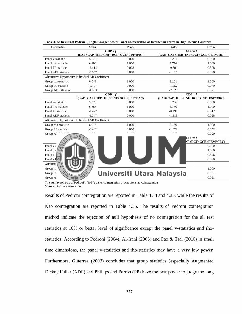
227
Table 4.35: Results of Pedroni ((Engle-Granger based) Panel Cointegration of Interaction Terms in High Income Countries
Estimates Stats. Prob. Stats. Prob.
GDP = f
(LAB+CAP+HED+INF+DCF+GCE+FDI*BAC)
GDP = f
(LAB+CAP+HED+INF+DCF+GCE+FDI*CRC)
Panel v-statistic 5.570 0.000
8.281 0.000
Panel rho-statistic 6.390 1.000
6.756 1.000
Panel PP statistic -2.414 0.008
-0.501 0.308
Panel ADF statistic -3.357 0.000
-1.911 0.028
Alternative Hypothesis: Individual AR Coefficient
Group rho-statistic 8.042 1.000
9.181 1.000
Group PP statistic -6.407 0.000
-1.652 0.049
Group ADF statistic -4.353 0.000
-2.025 0.021
GDP = f
(LAB+CAP+HED+INF+DCF+GCE+EXP*BAC)
GDP = f
(LAB+CAP+HED+INF+DCF+GCE+EXP*CRC)
Panel v-statistic 5.570 0.000
8.256 0.000
Panel rho-statistic 6.383 1.000
6.760 1.000
Panel PP statistic -2.422 0.008
-0.490 0.312
Panel ADF statistic -3.347 0.000
-1.918 0.028
Alternative Hypothesis: Individual AR Coefficient
Group rho-statistic 8.015 1.000
9.169 1.000
Group PP statistic -6.482 0.000
-1.622 0.052
Group ADF statistic -4.391 0.000
-2.062 0.020
GDP = f
(LAB+CAP+HED+INF+DCF+GCE+REM*BAC)
GDP = f
(LAB+CAP+HED+INF+DCF+GCE+REM*CRC)
Panel v-statistic 5.558 0.000
8.252 0.000
Panel rho-statistic 6.378 1.000
6.752 1.000
Panel PP statistic -2.406 0.008
-0.452 0.326
Panel ADF statistic -3.300 0.001
-1.878 0.030
Alternative Hypothesis: Individual AR Coefficient
Group rho-statistic 8.015 1.000
9.157 1.000
Group PP statistic -6.429 0.000
-1.636 0.051
Group ADF statistic -4.355 0.000 -2.031 0.021
The null hypothesis of Pedroni's (1997) panel cointegration procedure is no cointegration
Source: Author's estimation.
Results of Pedroni cointegration are reported in Table 4.34 and 4.35, while the results of
Kao cointegration are reported in Table 4.36. The results of Pedroni cointegration
method indicate the rejection of null hypothesis of no cointegration for the all test
statistics at 10% or better level of significance except the panel v-statistics and rho-
statistics. According to Pedroni (2004), Al-Irani (2006) and Pao & Tsai (2010) in small
time dimensions, the panel v-statistics and rho-statistics may have a very low power.
Furthermore, Guterrez (2003) concludes that group statistics (especially Augmented
Dickey Fuller (ADF) and Phillips and Perron (PP) have the best power to judge the long
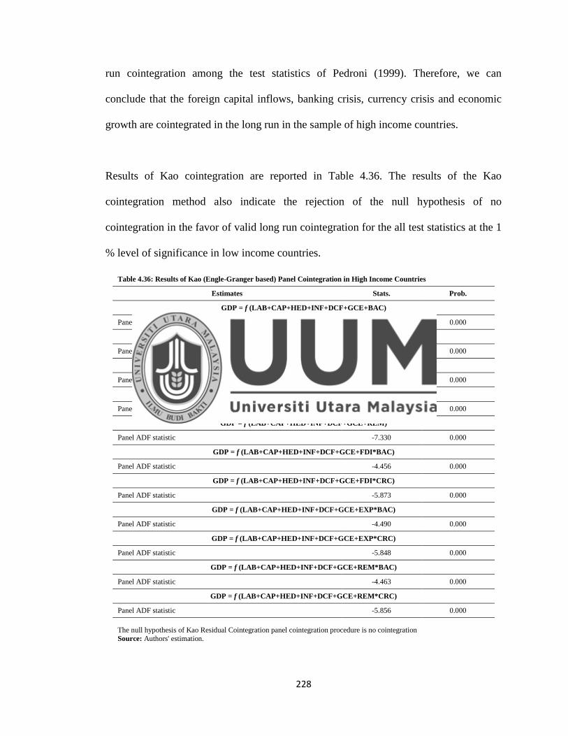
228
run cointegration among the test statistics of Pedroni (1999). Therefore, we can
conclude that the foreign capital inflows, banking crisis, currency crisis and economic
growth are cointegrated in the long run in the sample of high income countries.
Results of Kao cointegration are reported in Table 4.36. The results of the Kao
cointegration method also indicate the rejection of the null hypothesis of no
cointegration in the favor of valid long run cointegration for the all test statistics at the 1
% level of significance in low income countries.
Table 4.36: Results of Kao (Engle-Granger based) Panel Cointegration in High Income Countries
Estimates Stats. Prob.
GDP = f (LAB+CAP+HED+INF+DCF+GCE+BAC)
Panel ADF statistic -4.622 0.000
GDP = f (LAB+CAP+HED+INF+DCF+GCE+CRC)
Panel ADF statistic -5.630 0.000
GDP = f (LAB+CAP+HED+INF+DCF+GCE+FDI)
Panel ADF statistic -3.915 0.000
GDP = f (LAB+CAP+HED+INF+DCF+GCE+EXP)
Panel ADF statistic -5.682 0.000
GDP = f (LAB+CAP+HED+INF+DCF+GCE+REM)
Panel ADF statistic -7.330 0.000
GDP = f (LAB+CAP+HED+INF+DCF+GCE+FDI*BAC)
Panel ADF statistic -4.456 0.000
GDP = f (LAB+CAP+HED+INF+DCF+GCE+FDI*CRC)
Panel ADF statistic -5.873 0.000
GDP = f (LAB+CAP+HED+INF+DCF+GCE+EXP*BAC)
Panel ADF statistic -4.490 0.000
GDP = f (LAB+CAP+HED+INF+DCF+GCE+EXP*CRC)
Panel ADF statistic -5.848 0.000
GDP = f (LAB+CAP+HED+INF+DCF+GCE+REM*BAC)
Panel ADF statistic -4.463 0.000
GDP = f (LAB+CAP+HED+INF+DCF+GCE+REM*CRC)
Panel ADF statistic -5.856 0.000
The null hypothesis of Kao Residual Cointegration panel cointegration procedure is no cointegration
Source: Authors' estimation.

229
4.6.3 Long Run Analysis
After having the valid evidence of significant long run cointegration among considered
variables, the next step is to estimate the long run coefficients. We used fixed effect and
random effect methods to analyze the long run relationship. The Hausman test is used to
select the best preferable model between fixed effect and random effect models (Greene,
2000). The null hypothesis of Hausman test is that the country effects are uncorrelated
with the other regressors in the model (Hausman, 1978). If the country effect is
correlated (null hypothesis is rejected), a random effect model violating the basic
assumption of Gauss-Markov and produces the biased estimators. If null hypothesis, is
rejected, a fixed effect model is then preferred. Consequently, if the null hypothesis is
accepted, the estimated results of random effect model is then preferred, and one should
focus on results of random effect hereafter. In this section, we discuss the long run
impact and coefficients of different independent variables on economic growth in the
sample of high income countries.
Banking Crisis and Currency Crisis
The results which explain the long run impact of banking crisis and currency crisis on
economic growth is presented in Table 4.37. The results of banking crisis are reported in
model I whereas, the results of currency crisis are reported in model II. Results of both
models indicate that the prob value of Hausman test is significant (0.001) and (0.001),
which confirm the rejection of null hypothesis and concluded that the fixed effect model
is preferred over random effect model. Furthermore, the statistical value of Variance
Inflation factor (VIF) also suggest that there is no issue of multicollinearity exist among
the independent variables of estimated models. Results also indicate the negative and

230
significant impact of banking crisis and currency crisis on economic growth. It is
concluded that the banking and currency crises decrease the progress of the economic
development in high income countries.
Table 4.37: Long Run Results of Banking and Currency Crisis in High Income Countries
Variables
I II
FE RE FE RE
Coeff. Prob. VIF Coeff. Prob. VIF Coeff. Prob. VIF Coeff. Prob. VIF
α 17.842 0.000
17.023 0.000
18.165 0.000
17.304 0.000
LAB 0.286 0.000 1.078 0.317 0.000 1.101 0.256 0.000 1.073 0.290 0.000 1.096
CAP 0.199 0.000 2.682 0.196 0.000 2.792 0.202 0.000 2.662 0.200 0.000 2.773
HED 0.099 0.000 1.143 0.108 0.000 1.168 0.107 0.000 1.122 0.116 0.000 1.149
INF 0.001 0.019 1.227 0.001 0.009 1.215 0.001 0.044 1.261 0.001 0.023 1.248
DCF 0.007 0.230 1.073 0.009 0.100 1.085 0.004 0.522 1.035 0.006 0.277 1.045
GCE -0.022 0.230 2.961 -0.011 0.532 3.098 -0.018 0.342 2.970 -0.007 0.689 3.116
BAC -0.024 0.000 1.120 -0.024 0.000 1.116
CRC -0.013 0.028 1.060 -0.012 0.037 1.059
Adj. R2 0.998 0.565 0.998 0.560
Hausman
Stats. (Prob) 24.905 (0.001) 24.609 (0.001)
F-stats
(Prob.) 25678.03 (0.000) 114.854 (0.000) 25333.26 (0.000) 112.648 (0.000)
Source: Author's estimation.
Furthermore, the results of control variables show that the labor force, capital formation,
higher education development, domestic credit by the financial sector and inflation have
a positive impact on economic growth whereas, government consumption expenditure
has negative impact on economic growth in high income countries.
Foreign Direct Investment
The results which explain the long run impact of foreign direct investment and
interaction terms of banking and currency crisis with foreign direct investment on
economic growth is presented in Table 4.38. Model I, II and III show the results of foreign

231
direct investment, interaction of foreign direct investment and banking crisis and interaction of
foreign direct investment and currency crisis respectively. Results of all three models
indicate that the prob value of Hausman test is significant (0.001), (0.001) and (0.001),
which confirm the acceptance of null hypothesis and concluded that the fixed effect
model is preferred over random effect model. Furthermore, the statistical value of
Variance Inflation factor (VIF) also suggest that there is no issue of multicollinearity
exist among the independent variables of estimated models. Results indicate the positive
and significant impact of foreign direct investment on economic growth. The coefficient
of foreign direct investment is showing that the 1% increase in FDI causes the increase in
economic growth by 0.007%. This finding is consistent with the previous empirical studies.
Results of model II confirm that the impact of foreign direct investment on economic
growth becomes negative and significant in the presence of systemic banking crises.
Results of model III confirm that the impact of foreign direct investment on economic
growth remains positive and significant in the presence of currency crises. However, the
magnitude of the relationship is dragged down from 0.007 to 0.001. These findings
conclude that the banking and currency crisis are harmful for the relationship of foreign
direct investment and economic growth in high income countries.
Furthermore, the results of control variables show that the labor force, capital formation,
higher education development, domestic credit by the financial sector and inflation have
a positive impact on economic growth whereas, government consumption expenditure
has negative impact on economic growth in high income countries.
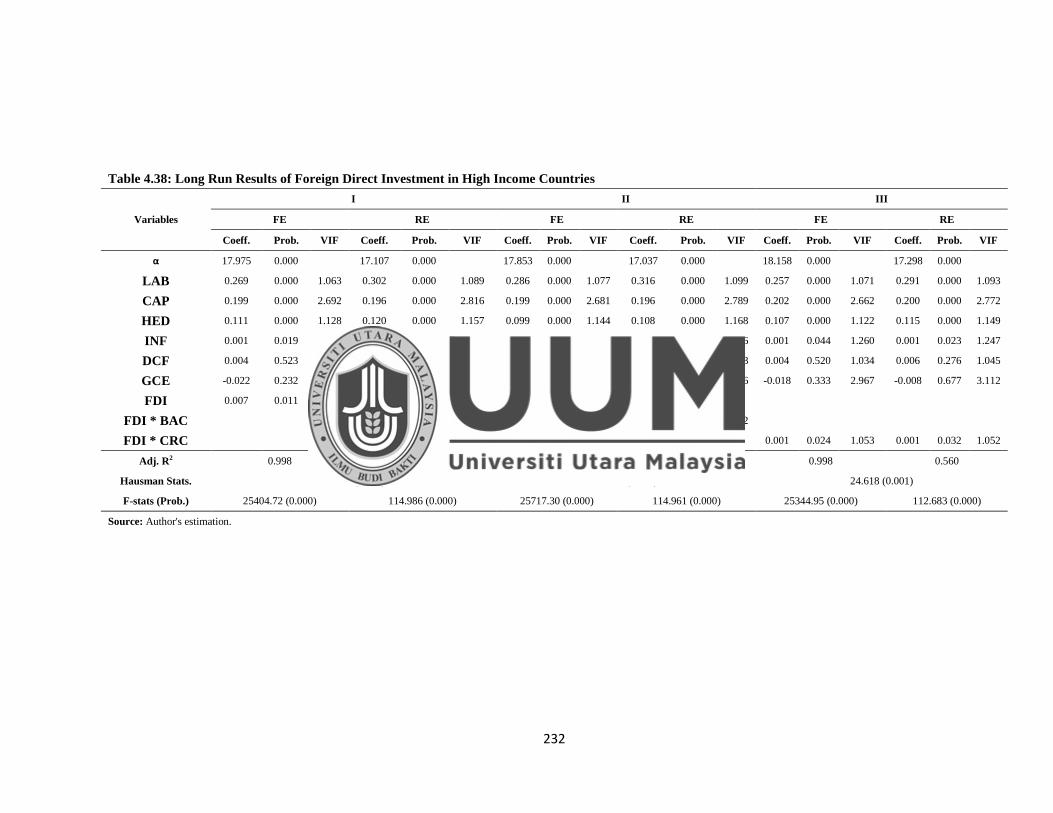
232
Table 4.38: Long Run Results of Foreign Direct Investment in High Income Countries
Variables
I II III
FE RE FE RE FE RE
Coeff. Prob. VIF Coeff. Prob. VIF Coeff. Prob. VIF Coeff. Prob. VIF Coeff. Prob. VIF Coeff. Prob. VIF
α 17.975 0.000
17.107 0.000
17.853 0.000
17.037 0.000
18.158 0.000
17.298 0.000
LAB 0.269 0.000 1.063 0.302 0.000 1.089 0.286 0.000 1.077 0.316 0.000 1.099 0.257 0.000 1.071 0.291 0.000 1.093
CAP 0.199 0.000 2.692 0.196 0.000 2.816 0.199 0.000 2.681 0.196 0.000 2.789 0.202 0.000 2.662 0.200 0.000 2.772
HED 0.111 0.000 1.128 0.120 0.000 1.157 0.099 0.000 1.144 0.108 0.000 1.168 0.107 0.000 1.122 0.115 0.000 1.149
INF 0.001 0.019 1.227 0.001 0.009 1.215 0.001 0.020 1.227 0.001 0.010 1.216 0.001 0.044 1.260 0.001 0.023 1.247
DCF 0.004 0.523 1.033 0.006 0.262 1.045 0.007 0.244 1.066 0.009 0.109 1.078 0.004 0.520 1.034 0.006 0.276 1.045
GCE -0.022 0.232 2.964 -0.011 0.531 3.123 -0.022 0.235 2.960 -0.011 0.540 3.096 -0.018 0.333 2.967 -0.008 0.677 3.112
FDI 0.007 0.011 1.055 0.007 0.005 1.060
FDI * BAC
-0.001 0.000 1.107 -0.001 0.000 1.102
FDI * CRC 0.001 0.024 1.053 0.001 0.032 1.052
Adj. R2 0.998 0.565 0.998 0.565 0.998 0.560
Hausman Stats. 24.023 (0.001) 24.912 (0.001) 24.618 (0.001)
F-stats (Prob.) 25404.72 (0.000) 114.986 (0.000) 25717.30 (0.000) 114.961 (0.000) 25344.95 (0.000) 112.683 (0.000)
Source: Author's estimation.
233
Export of Goods and Services
The results which explain the long run impact of exports of goods and services and
interaction terms of banking and currency crisis with exports of goods and services on
economic growth is presented in Table 4.39. Model I, II and III show the results of exports
of goods and services, interaction of exports and banking crisis and interaction of exports and
currency crisis respectively. Results of all three models indicate that the prob value of
Hausman test is significant (0.001), (0.001) and (0.001), which confirm the acceptance
of null hypothesis and concluded that the fixed effect model is preferred over random
effect model. Furthermore, the statistical value of Variance Inflation factor (VIF) also
suggest that there is no issue of multicollinearity exist among the independent variables
of estimated models. Results indicate the positive and significant impact of exports of
goods and services on economic growth. The coefficient of exports of goods and services
is showing that the 1% increase in exports causes the increase in economic growth by 0.130%.
This finding is consistent with the previous empirical studies. Results of model II confirm
that the impact of export on economic growth becomes negative and significant in the
presence of systemic banking crises. Results of model III confirm that the impact of
export on economic growth remains positive and significant in the presence of currency
crises. However, the magnitude of the relationship is dragged down from 0.130 to 0.001.
These findings conclude that the banking and currency crisis are harmful for the
relationship of export of goods and services and economic growth in high income
countries.

234
Table 4.39: Long Run Results of Exports in High Income Countries
Variables
I II III
FE RE FE RE FE RE
Coeff. Prob. VIF Coeff. Prob. VIF Coeff. Prob. VIF Coeff. Prob. VIF Coeff. Prob. VIF Coeff. Prob. VIF
α 15.1700 0.0000
14.5388 0.0000
17.8409 0.0000
17.0256 0.0000
18.1636 0.0000
17.3028 0.0000
LAB 0.3402 0.0000 1.0945 0.3654 0.0000 1.1571 0.2866 0.0000 1.0772 0.3171 0.0000 1.0997 0.2565 0.0000 1.0718 0.2905 0.0000 1.0940
CAP 0.1961 0.0000 2.6659 0.1945 0.0000 3.0632 0.1988 0.0000 2.6784 0.1965 0.0000 2.7870 0.2023 0.0000 2.6607 0.2001 0.0000 2.7713
HED 0.0782 0.0000 1.1632 0.0865 0.0000 1.3120 0.0994 0.0000 1.1407 0.1080 0.0000 1.1657 0.1065 0.0000 1.1229 0.1152 0.0000 1.1492
INF 0.0002 0.4331 1.2688 0.0002 0.5991 1.2613 0.0007 0.0197 1.2272 0.0008 0.0095 1.2156 0.0006 0.0436 1.2611 0.0007 0.0225 1.2481
DCF 0.0152 0.0057 1.0893 0.0186 0.0005 1.1026 0.0069 0.2329 1.0675 0.0094 0.1024 1.0793 0.0037 0.5233 1.0345 0.0062 0.2786 1.0454
GCE -0.0832 0.0000 3.3784 -0.0876 0.0000 4.4057 -0.0223 0.2260 2.9614 -0.0115 0.5245 3.0972 -0.0182 0.3284 2.9662 -0.0078 0.6694 3.1114
EXP 0.1300 0.0000 1.5761 0.1391 0.0000 2.0228
EXP * BAC
-0.0010 0.0002 1.1061 -0.0010 0.0002 1.1019
EXP * CRC 0.0005 0.0299 1.0543 0.0005 0.0402 1.0534
Adj. R2 0.998 0.687 0.998 0.567 0.980 0.559
Hausman. Stats. 25.843 (0.001) 24.906 (0.001) 24.617 (0.001)
F-stats (Prob.) 29255.67 (0.000) 194.570 (0.000) 25740.39 (0.000) 115.179 (0.000) 25329.52 (0.000) 112.542 (0.000)
Source: Author's estimation.
235
Furthermore, the results of control variables show that the labor force, capital formation,
higher education development, domestic credit by the financial sector and inflation have
a positive impact on economic growth whereas, government consumption expenditure
has negative impact on economic growth in high income countries.
Workers’ Remittances
The results which explain the long run impact of workers‘ remittances and interaction
terms of banking and currency crisis with workers‘ remittances on economic growth is
presented in Table 4.40. Model I, II and III show the results of workers‘ remittances,
interaction of workers‘ remittances and banking crisis and interaction of workers‘
remittances and currency crisis respectively. Results of all three models indicate that the
prob value of Hausman test is significant (0.001), (0.001) and (0.001), which confirm
the acceptance of null hypothesis and concluded that the fixed effect model is preferred
over random effect model. Furthermore, the statistical value of Variance Inflation factor
(VIF) also suggest that there is no issue of multicollinearity exist among the independent
variables of estimated models. Results indicate the positive and significant impact of
workers‘ remittances on economic growth. This finding is consistent with the previous
empirical studies. The coefficient of remittances is showing that the 1% increase in REM causes
the increase in economic growth by 0.019%. Results of model II confirm that the impact of
export on economic growth becomes negative and significant in the presence of
systemic banking crises. Results of model III confirm that the impact of export on
economic growth remains positive and significant in the presence of currency crises.
However, the magnitude of the relationship is dragged down from 0.019% to 0.001.
These findings conclude that the banking and currency crisis are harmful for the
relationship of workers‘ remittances and economic growth in high income countries.

236
Table 4.40: Long Run Results of Remittances in High Income Countries
Variables
I II III
FE RE FE RE FE RE
Coeff. Prob. VIF Coeff. Prob. VIF Coeff. Prob. VIF Coeff. Prob. VIF Coeff. Prob. VIF Coeff. Prob. VIF
α 16.722 0.000
15.840 0.000
17.818 0.000
17.008 0.000
18.162 0.000
17.300 0.000
LAB 0.329 0.000 1.125 0.362 0.000 1.143 0.289 0.000 1.078 0.319 0.000 1.100 0.257 0.000 1.072 0.291 0.000 1.094
CAP 0.192 0.000 2.714 0.189 0.000 2.853 0.198 0.000 2.682 0.196 0.000 2.790 0.202 0.000 2.660 0.200 0.000 2.771
HED 0.086 0.000 1.184 0.093 0.000 1.228 0.100 0.000 1.137 0.108 0.000 1.162 0.106 0.000 1.124 0.115 0.000 1.150
INF 0.001 0.032 1.230 0.001 0.019 1.217 0.001 0.021 1.228 0.001 0.010 1.216 0.001 0.040 1.258 0.001 0.020 1.245
DCF 0.018 0.004 1.265 0.022 0.000 1.271 0.007 0.239 1.060 0.009 0.105 1.072 0.004 0.510 1.037 0.006 0.271 1.048
GCE -0.024 0.187 2.963 -0.014 0.426 3.157 -0.022 0.234 2.960 -0.011 0.539 3.095 -0.019 0.319 2.965 -0.008 0.656 3.110
REM 0.019 0.000 1.440 0.021 0.000 1.430
REM * BAC
-0.001 0.000 1.094 -0.001 0.000 1.090
REM * CRC 0.001 0.041 1.052 0.001 0.055 1.050
Adj. R2 0.998 0.590 0.998 0.567 0.998 0.559
Hausman. Stats. 23.700 (0.001) 24.897 (0.001) 24.617 (0.001)
F-stats (Prob.) 26518.72 (0.000) 127.467 (0.000) 25840.55 (0.000) 115.821 (0.000) 25305.60 (0.000) 112.371 (0.000)
Source: Author's estimation.

237
Furthermore, the results of control variables show that the labor force, capital formation,
higher education development, domestic credit by the financial sector and inflation have
a positive impact on economic growth whereas, government consumption expenditure
has negative impact on economic growth in high income countries.
4.7 Aggregate Results of 96 Countries
In this section, we present the aggregate results of empirical estimations of 96 countries
and further discuss these results in the theoretical and conceptual context.
4.7.1 Unit Root Analyses
Table 4.41: Results of Stationary Analyses for Upper Middle Income Countries
Variables
Im, Pesaran and Shin
I(0) I(1)
C C&T C C&T
GDP 17.091 5.166 -7.878*** -9.138***
LAB 14.092 2.701 -6.531*** -5.546***
CAP 14.101 4.510 -10.799*** -11.578***
HED 3.2689 2.2214 -8.227*** -8.028***
INF 14.7102 1.6281 -29.530*** -24.723***
DCF 4.032 -1.055 -13.630*** -8.532***
GCE 18.554 5.406 -6.670*** -7.555***
FDI 1.155 -0.814 -19.908*** -15.357***
EXP 16.816 0.558 -19.009*** -20.715***
REM 8.461 -0.101 -13.460*** -10.381***
EXD 15.699 9.515 -3.531*** -3.854***
*, **, *** indicates significance level respectively at 1%, 5% and 10%.
Source: Authors' estimation.
We use, Im, Pesaran and Shin (2003) unit root test to analyze the stationary properties of
our considered variables. The IPS test considers the unobserved heterogeneity among
the cross sections and also eliminates the issues of serial correlation. The IPS unit root
test has the best properties to judge the problem of a unit root in the small sample. The
238
desirable results for unit root test include that the variables should be non-stationary at
the level and become stationary at the first difference. Table 4.41 represents the results
of stationary analyses for the aggregate sample of 96 countries. We first, employed these
tests on the level of each variable and then applied to the first difference. In both
estimation procedures of level and first difference, we also analyze the results in two
dimensions, i.e. with constant and with constant and trend. Results indicate that all the
variables are non-stationary at level and become stationary at first difference. These
results confirm that there is no problem of unit root in our variables and we can further
use these variables for the long run estimations.
4.7.2 Cointegration Analyses
After having the confirmation from unit root test that our variables have a stationary
properties of I(1) which is the requirement to perform panel cointegration techniques,
we applied two methods of panel cointegration i.e. Pedroni cointegration (1999) and
Kao cointegration (1999) to analyze the long run relationship among foreign capital
inflows, banking crisis, currency crisis and economic growth in the aggregate sample of
96 countries. These tests are based on the two-step residual based cointegration tests of
Engle-Granger (1987). The Pedroni cointegration based on a seven statistical value. The
Pedroni cointegration is useful to control the biasness of country size and also solve the
issues of heterogeneity (Das & Choudhary, 2011). The Kao cointegration method
follows the same basic approached as used in the Pedroni cointegration, but also control
the issues of cross-section specific intercepts and homogenous coefficients.
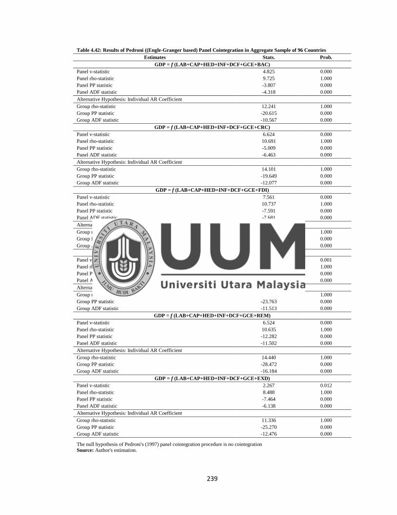
239
Table 4.42: Results of Pedroni ((Engle-Granger based) Panel Cointegration in Aggregate Sample of 96 Countries
Estimates Stats. Prob.
GDP = f (LAB+CAP+HED+INF+DCF+GCE+BAC)
Panel v-statistic 4.825 0.000
Panel rho-statistic 9.725 1.000
Panel PP statistic -3.807 0.000
Panel ADF statistic -4.318 0.000
Alternative Hypothesis: Individual AR Coefficient
Group rho-statistic 12.241 1.000
Group PP statistic -20.615 0.000
Group ADF statistic -10.567 0.000
GDP = f (LAB+CAP+HED+INF+DCF+GCE+CRC)
Panel v-statistic 6.624 0.000
Panel rho-statistic 10.691 1.000
Panel PP statistic -5.009 0.000
Panel ADF statistic -6.463 0.000
Alternative Hypothesis: Individual AR Coefficient
Group rho-statistic 14.101 1.000
Group PP statistic -19.649 0.000
Group ADF statistic -12.077 0.000
GDP = f (LAB+CAP+HED+INF+DCF+GCE+FDI)
Panel v-statistic 7.561 0.000
Panel rho-statistic 10.737 1.000
Panel PP statistic -7.591 0.000
Panel ADF statistic -7.681 0.000
Alternative Hypothesis: Individual AR Coefficient
Group rho-statistic 14.223 1.000
Group PP statistic -24.768 0.000
Group ADF statistic -14.568 0.000
GDP = f (LAB+CAP+HED+INF+DCF+GCE+EXP)
Panel v-statistic 3.147 0.001
Panel rho-statistic 11.086 1.000
Panel PP statistic -7.458 0.000
Panel ADF statistic -8.688 0.000
Alternative Hypothesis: Individual AR Coefficient
Group rho-statistic 14.636 1.000
Group PP statistic -23.763 0.000
Group ADF statistic -11.513 0.000
GDP = f (LAB+CAP+HED+INF+DCF+GCE+REM)
Panel v-statistic 6.524 0.000
Panel rho-statistic 10.635 1.000
Panel PP statistic -12.282 0.000
Panel ADF statistic -11.502 0.000
Alternative Hypothesis: Individual AR Coefficient
Group rho-statistic 14.440 1.000
Group PP statistic -28.472 0.000
Group ADF statistic -16.184 0.000
GDP = f (LAB+CAP+HED+INF+DCF+GCE+EXD)
Panel v-statistic 2.267 0.012
Panel rho-statistic 8.488 1.000
Panel PP statistic -7.464 0.000
Panel ADF statistic -6.138 0.000
Alternative Hypothesis: Individual AR Coefficient
Group rho-statistic 11.336 1.000
Group PP statistic -25.270 0.000
Group ADF statistic -12.476 0.000
The null hypothesis of Pedroni's (1997) panel cointegration procedure is no cointegration Source: Author's estimation.

240
Results of Pedroni cointegration are reported in Table 4.42 and 4.43, while the results of Kao
cointegration are reported in table 4.44. The results of Pedroni cointegration method indicate the
rejection of null hypothesis of no cointegration for the all test statistics at 10% or better level of
significance except the panel v-statistics and rho-statistics. According to Pedroni (2004), Al-Irani
(2006) and Pao & Tsai (2010) in small time dimensions, the panel v-statistics and rho-statistics may
have a very low power. Furthermore, Guterrez (2003) concludes that group statistics (especially
Augmented Dickey Fuller (ADF) and Phillips and Perron (PP) have the best power to judge the long
run cointegration among the test statistics of Pedroni (1999). Therefore, we can conclude that the
foreign capital inflows, banking crisis, currency crisis and economic growth are cointegrated in the
long run in the aggregate sample of 96 countries.
Table 4.43: Results of Pedroni ((Engle-Granger based) Panel Cointegration of Interaction Terms in Aggregate Sample of 96 Countries
Estimates Stats. Prob. Stats. Prob.
GDP = f
(LAB+CAP+HED+INF+DCF+GCE+FDI*BAC)
GDP = f
(LAB+CAP+HED+INF+DCF+GCE+FDI*CRC)
Panel v-statistic 4.761 0.000
6.635 0.000
Panel rho-statistic 9.689 1.000
10.656 1.000
Panel PP statistic -3.730 0.000
-4.993 0.000
Panel ADF statistic -4.246 0.000
-6.159 0.000
Alternative Hypothesis: Individual AR Coefficient
Group rho-statistic 12.225 1.000
14.105 1.000
Group PP statistic -20.390 0.000
-19.747 0.000
Group ADF statistic -10.433 0.000
-11.903 0.000
GDP = f
(LAB+CAP+HED+INF+DCF+GCE+EXP*BAC)
GDP = f
(LAB+CAP+HED+INF+DCF+GCE+EXP*CRC)
Panel v-statistic 4.825 0.000
6.612 0.000
Panel rho-statistic 9.727 1.000
10.685 1.000
Panel PP statistic -3.783 0.000
-5.024 0.000
Panel ADF statistic -4.283 0.000
-6.464 0.000
Alternative Hypothesis: Individual AR Coefficient
Group rho-statistic 12.236 1.000
14.092 1.000
Group PP statistic -20.587 0.000
-19.674 0.000
Group ADF statistic -10.550 0.000
-12.057 0.000
GDP = f
(LAB+CAP+HED+INF+DCF+GCE+REM*BAC)
GDP = f
(LAB+CAP+HED+INF+DCF+GCE+REM*CRC)
Panel v-statistic 4.786 0.000
6.616 0.000
Panel rho-statistic 9.749 1.000
10.628 1.000
Panel PP statistic -3.716 0.000
-4.940 0.000
Panel ADF statistic -4.211 0.000
-6.063 0.000
Alternative Hypothesis: Individual AR Coefficient
Group rho-statistic 12.243 1.000
14.083 1.000
Group PP statistic -20.557 0.000
-19.623 0.000
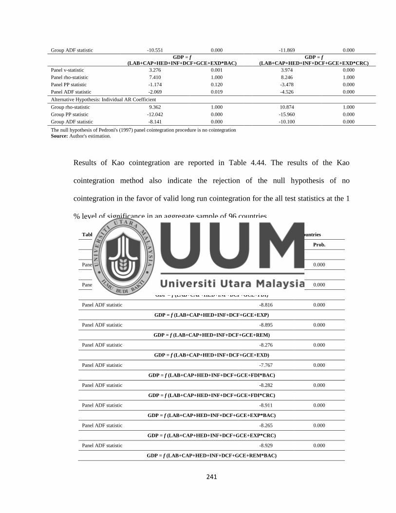
241
Group ADF statistic -10.551 0.000
-11.869 0.000
GDP = f
(LAB+CAP+HED+INF+DCF+GCE+EXD*BAC)
GDP = f
(LAB+CAP+HED+INF+DCF+GCE+EXD*CRC)
Panel v-statistic 3.276 0.001
3.974 0.000
Panel rho-statistic 7.410 1.000
8.246 1.000
Panel PP statistic -1.174 0.120
-3.478 0.000
Panel ADF statistic -2.069 0.019
-4.526 0.000
Alternative Hypothesis: Individual AR Coefficient
Group rho-statistic 9.362 1.000
10.874 1.000
Group PP statistic -12.042 0.000
-15.960 0.000
Group ADF statistic -8.141 0.000 -10.100 0.000
The null hypothesis of Pedroni's (1997) panel cointegration procedure is no cointegration
Source: Author's estimation.
Results of Kao cointegration are reported in Table 4.44. The results of the Kao
cointegration method also indicate the rejection of the null hypothesis of no
cointegration in the favor of valid long run cointegration for the all test statistics at the 1
% level of significance in an aggregate sample of 96 countries.
Table 4.44: Results of Kao (Engle-Granger based) Panel Cointegration in Aggregate Sample of 96 Countries
Estimates Stats. Prob.
GDP = f (LAB+CAP+HED+INF+DCF+GCE+BAC)
Panel ADF statistic -8.504 0.000
GDP = f (LAB+CAP+HED+INF+DCF+GCE+CRC)
Panel ADF statistic -8.644 0.000
GDP = f (LAB+CAP+HED+INF+DCF+GCE+FDI)
Panel ADF statistic -8.816 0.000
GDP = f (LAB+CAP+HED+INF+DCF+GCE+EXP)
Panel ADF statistic -8.895 0.000
GDP = f (LAB+CAP+HED+INF+DCF+GCE+REM)
Panel ADF statistic -8.276 0.000
GDP = f (LAB+CAP+HED+INF+DCF+GCE+EXD)
Panel ADF statistic -7.767 0.000
GDP = f (LAB+CAP+HED+INF+DCF+GCE+FDI*BAC)
Panel ADF statistic -8.282 0.000
GDP = f (LAB+CAP+HED+INF+DCF+GCE+FDI*CRC)
Panel ADF statistic -8.911 0.000
GDP = f (LAB+CAP+HED+INF+DCF+GCE+EXP*BAC)
Panel ADF statistic -8.265 0.000
GDP = f (LAB+CAP+HED+INF+DCF+GCE+EXP*CRC)
Panel ADF statistic -8.929 0.000
GDP = f (LAB+CAP+HED+INF+DCF+GCE+REM*BAC)

242
Panel ADF statistic -8.324 0.000
GDP = f (LAB+CAP+HED+INF+DCF+GCE+REM*CRC)
Panel ADF statistic -8.868 0.000
GDP = f (LAB+CAP+HED+INF+DCF+GCE+EXD*BAC)
Panel ADF statistic -8.780 0.000
GDP = f (LAB+CAP+HED+INF+DCF+GCE+EXD*CRC)
Panel ADF statistic -9.482 0.000
The null hypothesis of Kao Residual Cointegration panel cointegration procedure is no cointegration
Source: Authors' estimation.
4.7.3 Long Run Analysis
After having the valid evidence of significant long run cointegration among considered
variables, the next step is to estimate the long run coefficients. We used fixed effect and
random effect methods to analyze the long run relationship. The Hausman test is used to
select the best preferable model between fixed effect and random effect models (Greene,
2000). The null hypothesis of Hausman test is that the country effects are uncorrelated
with the other regressors in the model (Hausman, 1978). If the country effect is
correlated (null hypothesis is rejected), a random effect model violating the basic
assumption of Gauss-Markov and produces the biased estimators. If null hypothesis, is
rejected, a fixed effect model is then preferred. Consequently, if the null hypothesis is
accepted, the estimated results of random effect model is then preferred, and one should
focus on results of random effect hereafter. In this section, we discuss the long run
impact and coefficients of different independent variables on economic growth in the
aggregate sample of 96 countries.

243
Banking Crisis and Currency Crisis
The results which explain the long run impact of banking crisis and currency crisis on
economic growth is presented in Table 4.45. The results of banking crisis are reported in
model I whereas, the results of currency crisis are reported in model II. Results of both
models indicate that the prob value of Hausman test is significant (0.000) and (0.000),
which confirm the acceptance of null hypothesis and concluded that the fixed effect
model is preferred over random effect model. Furthermore, the statistical value of
Variance Inflation factor (VIF) also suggest that there is no issue of multicollinearity
exist among the independent variables of estimated models. Results also indicate the
negative and significant impact of banking crisis and currency crisis on economic
growth. It is concluded that the banking and currency crises decrease the progress of the
economic development. Results also conclude that the banking crisis and currency
crisis, both have the equal/same negative impact on economic growth.
Table 4.45: Long Run Results of Banking and Currency Crisis in Aggregate Sample of 96 Countries
Variables
I II
FE RE FE RE
Coeff. Prob. VIF Coeff. Prob. VIF Coeff. Prob. VIF Coeff. Prob. VIF
α 15.120 0.000 14.324 0.000 15.153 0.000 14.382 0.000
LAB 0.279 0.000 1.249 0.316 0.000 1.261 0.273 0.000 1.251 0.310 0.000 1.259
CAP 0.155 0.000 2.383 0.155 0.000 2.553 0.157 0.000 2.367 0.158 0.000 2.522
HED 0.026 0.001 1.323 0.024 0.001 1.349 0.029 0.000 1.312 0.027 0.000 1.334
INF 0.001 0.048 1.078 0.001 0.066 1.077 0.006 0.266 1.071 0.006 0.336 1.070
DCF 0.057 0.000 1.120 0.060 0.000 1.142 0.052 0.000 1.091 0.055 0.000 1.110
GCE 0.100 0.000 2.384 0.104 0.000 2.578 0.104 0.000 2.401 0.109 0.000 2.580
BAC -0.024 0.000 1.067 -0.025 0.000 1.067
CRC -0.024 0.000 1.029 -0.024 0.000 1.031
Adj. R2 0.998 0.587 0.998 0.587
Hausman Stats.
(Prob.) 64.806 (0.000) 65.116 (0.000)
F-stats (Prob.) 21376.05 (0.000) 369.343 (0.000) 21517.35 (0.000) 368.0664 (0.000)
Source: Authors' estimation.

244
Furthermore, the results of control variables show that the labor force, capital formation,
higher education development, domestic credit by financial sector, inflation and
government consumption expenditure have significant positive impact on economic
growth in an aggregate sample of 96 countries.
Foreign Direct Investment
The results which explain the long run impact of foreign direct investment and
interaction terms of banking and currency crisis with foreign direct investment on
economic growth is presented in Table 4.46. Model I, II and III show the results of
foreign direct investment, interaction of foreign direct investment and banking crisis and
interaction of foreign direct investment and currency crisis respectively. Results of all
three models indicate that the prob value of Hausman test is significant (0.000), (0.000)
and (0.000), which confirm the acceptance of null hypothesis and concluded that the
fixed effect model is preferred over random effect model. Furthermore, the statistical
value of Variance Inflation factor (VIF) also suggest that there is no issue of
multicollinearity exist among the independent variables of estimated models. Results
indicate the positive and significant impact of foreign direct investment on economic
growth. The coefficient of foreign direct investment is showing that the 1% increase in
FDI causes the increase in economic growth by 0.006%. This finding is consistent with
the previous empirical studies of (Vudayagiri N Balasubramanyam et al., 1999;
Nair‐Reichert and Weinhold, 2001; Choe, 2003; Li and Liu, 2005; Rabiei and Masoudi,
2012; Omri and Kahouli, 2014; Olayemi, 2015; Yusoff and Nuh, 2015). Results of model
II confirm that the impact of FDI on economic growth becomes significantly negative in the

245
presence of systemic banking crises. Results of model III further confirm that the impact of
FDI on economic growth remains positive and significant in the presence of currency
crises. However, the magnitude of the relationship is dropped down from 0.006 to 0.001.
These findings conclude that the banking and currency crisis are harmful for the
relationship of export and economic growth in aggregate sample.
Furthermore, the results of control variables show that the labor force, capital formation,
higher education development, domestic credit by financial sector, inflation and
government consumption expenditure have a positive impact on economic growth in
aggregate sample.
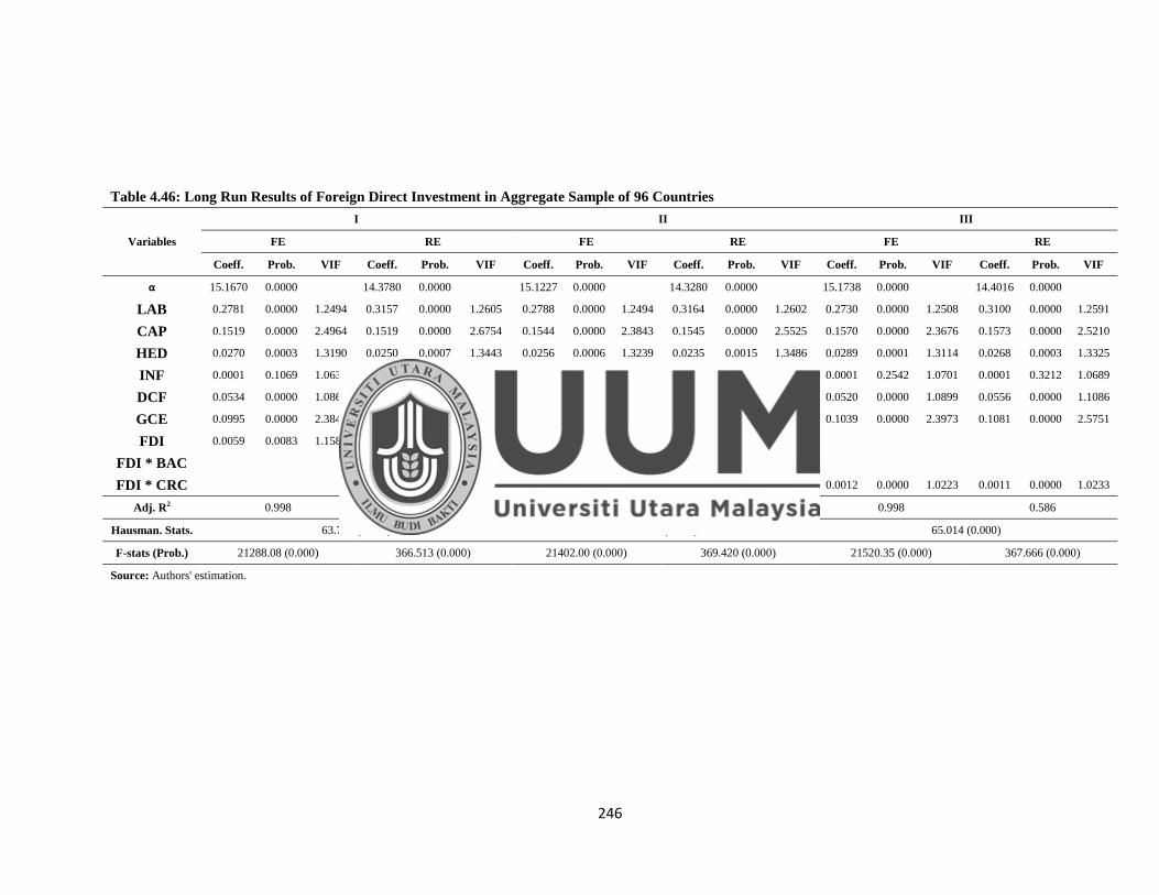
246
Table 4.46: Long Run Results of Foreign Direct Investment in Aggregate Sample of 96 Countries
Variables
I II III
FE RE FE RE FE RE
Coeff. Prob. VIF Coeff. Prob. VIF Coeff. Prob. VIF Coeff. Prob. VIF Coeff. Prob. VIF Coeff. Prob. VIF
α 15.1670 0.0000 14.3780 0.0000 15.1227 0.0000 14.3280 0.0000 15.1738 0.0000 14.4016 0.0000
LAB 0.2781 0.0000 1.2494 0.3157 0.0000 1.2605 0.2788 0.0000 1.2494 0.3164 0.0000 1.2602 0.2730 0.0000 1.2508 0.3100 0.0000 1.2591
CAP 0.1519 0.0000 2.4964 0.1519 0.0000 2.6754 0.1544 0.0000 2.3843 0.1545 0.0000 2.5525 0.1570 0.0000 2.3676 0.1573 0.0000 2.5210
HED 0.0270 0.0003 1.3190 0.0250 0.0007 1.3443 0.0256 0.0006 1.3239 0.0235 0.0015 1.3486 0.0289 0.0001 1.3114 0.0268 0.0003 1.3325
INF 0.0001 0.1069 1.0637 0.0001 0.1463 1.0624 0.0001 0.0520 1.0738 0.0001 0.0717 1.0726 0.0001 0.2542 1.0701 0.0001 0.3212 1.0689
DCF 0.0534 0.0000 1.0863 0.0570 0.0000 1.1071 0.0567 0.0000 1.1176 0.0605 0.0000 1.1388 0.0520 0.0000 1.0899 0.0556 0.0000 1.1086
GCE 0.0995 0.0000 2.3845 0.1041 0.0000 2.5776 0.0997 0.0000 2.3845 0.1045 0.0000 2.5760 0.1039 0.0000 2.3973 0.1081 0.0000 2.5751
FDI 0.0059 0.0083 1.1582 0.0060 0.0064 1.1757
FDI * BAC
-0.0012 0.0001 1.0618 -0.0012 0.0000 1.0620
FDI * CRC 0.0012 0.0000 1.0223 0.0011 0.0000 1.0233
Adj. R2 0.998 0.586 0.998 0.587 0.998 0.586
Hausman. Stats. 63.723 (0.000) 64.781 (0.000) 65.014 (0.000)
F-stats (Prob.) 21288.08 (0.000) 366.513 (0.000) 21402.00 (0.000) 369.420 (0.000) 21520.35 (0.000) 367.666 (0.000)
Source: Authors' estimation.
247
Export of Goods and Services
The results which explain the long run impact of exports of goods and services and
interaction terms of banking and currency crisis with exports of goods and services on
economic growth is presented in Table 4.47. Model I, II and III show the results of exports
of goods and services, interaction of exports and banking crisis and interaction of exports and
currency crisis respectively. Results of all three models indicate that the prob value of
Hausman test is significant (0.000), (0.000) and (0.000), which confirm the acceptance
of null hypothesis and concluded that the fixed effect model is preferred over random
effect model. Furthermore, the statistical value of Variance Inflation factor (VIF) also
suggest that there is no issue of multicollinearity exist among the independent variables
of estimated models. Results indicate the positive and significant impact of exports of
goods and services on economic growth. The coefficient of exports of goods and services
is showing that the 1% increase in exports causes the increase in economic growth by 0.156%.
This finding is consistent with the previous empirical studies. Results of model II confirm that
the impact of exports on economic growth becomes significantly negative in the presence of
systemic banking crises. Results of model III further confirm that the impact of exports of
goods and services on economic growth remains positive and significant in the presence
of currency crises. However, the magnitude of the relationship is dropped down from
0.156 to 0.0012. These findings conclude that the banking and currency crisis are harmful for
the relationship of export and economic growth in aggregate sample.
Furthermore, the results of control variables show that the labor force, capital formation,
higher education development, domestic credit by financial sector, inflation and
government consumption expenditure have a positive impact on economic growth in
aggregate sample.

248
Table 4.47: Long Run Results of Exports in Aggregate Sample of 96 Countries
Variables
I II III
FE RE FE RE FE RE
Coeff. Prob. VIF Coeff. Prob. VIF Coeff. Prob. VIF Coeff. Prob. VIF Coeff. Prob. VIF Coeff. Prob. VIF
α 13.3184 0.0000 13.0000 0.0000 15.1230 0.0000 14.3280 0.0000 15.1741 0.0000 14.4024 0.0000
LAB 0.3144 0.0000 1.2561 0.3352 0.0000 1.3130 0.2788 0.0000 1.2494 0.3164 0.0000 1.2603 0.2727 0.0000 1.2510 0.3097 0.0000 1.2593
CAP 0.1139 0.0000 2.5658 0.1135 0.0000 3.0018 0.1545 0.0000 2.3829 0.1547 0.0000 2.5514 0.1571 0.0000 2.3675 0.1574 0.0000 2.5207
HED 0.0257 0.0002 1.3119 0.0245 0.0003 1.4055 0.0257 0.0006 1.3232 0.0236 0.0014 1.3481 0.0290 0.0001 1.3115 0.0269 0.0002 1.3325
INF 0.0001 0.2800 1.0642 0.0004 0.4432 1.0628 0.0001 0.0511 1.0745 0.0001 0.0704 1.0734 0.0001 0.2565 1.0702 0.0001 0.3238 1.0690
DCF 0.0461 0.0000 1.0951 0.0485 0.0000 1.1548 0.0567 0.0000 1.1179 0.0605 0.0000 1.1392 0.0520 0.0000 1.0902 0.0556 0.0000 1.1089
GCE 0.0490 0.0000 2.5389 0.0459 0.0000 3.1612 0.0996 0.0000 2.3845 0.1043 0.0000 2.5764 0.1040 0.0000 2.3982 0.1083 0.0000 2.5758
EXP 0.1563 0.0000 1.6577 0.1566 0.0000 2.0233
EXP * BAC
-0.0010 0.0001 1.0617 -0.0011 0.0000 1.0620
EXP * CRC 0.0010 0.0000 1.0241 0.0010 0.0000 1.0252
Adj. R2 0.998 0.693 0.998 0.587 0.998 0.586
Hausman. Stats. 82.303 (0.000) 64.780 (0.000) 65.071 (0.000)
F-stats (Prob.) 25452.65 (0.000) 585.892 (0.000) 21396.54 (0.000) 369.425 (0.000) 21524.66 (0.000) 367.707 (0.000)
Source: Authors' estimation.

249
Workers’ Remittances
The results which explain the long run impact of workers‘ remittances and interaction
terms of banking and currency crisis with workers‘ remittances on economic growth is
presented in Table 4.48. Model I, II and III show the results of workers‘ remittances,
interaction of workers‘ remittances and banking crisis and interaction of workers‘
remittances and currency crisis respectively. Results of all three models indicate that the
prob. value of Hausman test is significant (0.000), (0.000) and (0.000), which confirm
the acceptance of null hypothesis and concluded that the fixed effect model is preferred
over random effect model. Furthermore, the statistical value of Variance Inflation factor
(VIF) also suggest that there is no issue of multicollinearity exist among the independent
variables of estimated models. Results indicate the positive and significant impact of
workers‘ remittances on economic growth. The coefficient of REM is showing that the 1%
increase in remittances causes the increase in economic growth by 0.009%. This finding is
consistent with the previous empirical studies. Results of model II confirm that the impact of
workers‘ remittances on economic growth becomes significantly negative in the presence of
systemic banking crises. Results of model III further confirm that the impact of remittances on
economic growth remains positive and significant in the presence of currency crises.
However, the magnitude of the relationship is dropped down from 0.009 to 0.0012.
These findings conclude that the banking and currency crisis are harmful for the relationship of
workers‘ remittances and economic growth in aggregate sample.
Furthermore, the results of control variables show that the labor force, capital
formation, higher education development, domestic credit by financial sector, inflation
and government consumption expenditure have a positive impact on economic growth
in aggregate sample.
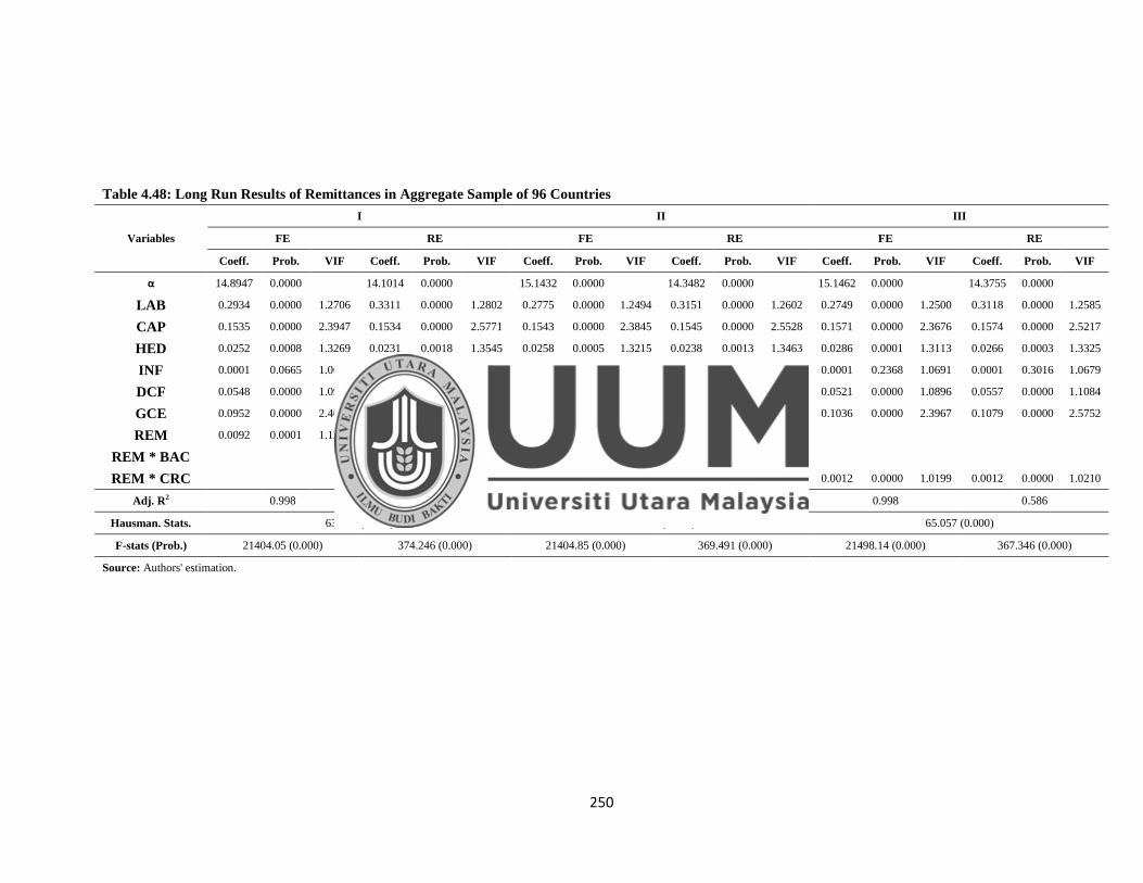
250
Table 4.48: Long Run Results of Remittances in Aggregate Sample of 96 Countries
Variables
I II III
FE RE FE RE FE RE
Coeff. Prob. VIF Coeff. Prob. VIF Coeff. Prob. VIF Coeff. Prob. VIF Coeff. Prob. VIF Coeff. Prob. VIF
α 14.8947 0.0000 14.1014 0.0000 15.1432 0.0000 14.3482 0.0000 15.1462 0.0000 14.3755 0.0000
LAB 0.2934 0.0000 1.2706 0.3311 0.0000 1.2802 0.2775 0.0000 1.2494 0.3151 0.0000 1.2602 0.2749 0.0000 1.2500 0.3118 0.0000 1.2585
CAP 0.1535 0.0000 2.3947 0.1534 0.0000 2.5771 0.1543 0.0000 2.3845 0.1545 0.0000 2.5528 0.1571 0.0000 2.3676 0.1574 0.0000 2.5217
HED 0.0252 0.0008 1.3269 0.0231 0.0018 1.3545 0.0258 0.0005 1.3215 0.0238 0.0013 1.3463 0.0286 0.0001 1.3113 0.0266 0.0003 1.3325
INF 0.0001 0.0665 1.0685 0.0001 0.0893 1.0675 0.0001 0.0525 1.0733 0.0001 0.0727 1.0722 0.0001 0.2368 1.0691 0.0001 0.3016 1.0679
DCF 0.0548 0.0000 1.0919 0.0586 0.0000 1.1135 0.0566 0.0000 1.1146 0.0603 0.0000 1.1359 0.0521 0.0000 1.0896 0.0557 0.0000 1.1084
GCE 0.0952 0.0000 2.4048 0.0993 0.0000 2.6184 0.0999 0.0000 2.3846 0.1046 0.0000 2.5761 0.1036 0.0000 2.3967 0.1079 0.0000 2.5752
REM 0.0092 0.0001 1.1228 0.0100 0.0000 1.1354
REM * BAC
-0.0012 0.0001 1.0573 -0.0013 0.0000 1.0576
REM * CRC 0.0012 0.0000 1.0199 0.0012 0.0000 1.0210
Adj. R2 0.998 0.591 0.998 0.586 0.998 0.586
Hausman. Stats. 63.336 (0.000) 64.735 (0.000) 65.057 (0.000)
F-stats (Prob.) 21404.05 (0.000) 374.246 (0.000) 21404.85 (0.000) 369.491 (0.000) 21498.14 (0.000) 367.346 (0.000)
Source: Authors' estimation.
251
External Debt
The results which explain the long run impact of external debt and interaction terms of
banking and currency crisis with external debt on economic growth is presented in Table
4.49. Model I, II and III show the results of external debt, interaction of external debt and
banking crisis and interaction of external debt and currency crisis respectively. Results of all
three models indicate that the prob value of Hausman test is significant (0.000), (0.000)
and (0.000), which confirm the acceptance of null hypothesis and concluded that the
fixed effect model is preferred over random effect model. Furthermore, the statistical
value of Variance Inflation factor (VIF) also suggest that there is no issue of
multicollinearity exist among the independent variables of estimated models. Results
indicate the positive and significant impact of external debt on economic growth. This
finding is consistent with the previous empirical studies. The coefficient of external debt is
showing that the 1% increase in external debt causes the increase in economic growth by
0.034%. Results of model II confirm that the impact of external debt on economic growth
becomes negative, but insignificant in the presence of systemic banking crises. Results of model
III further confirm that the impact of external debt on economic growth remain positive
and significant in the presence of currency crises. However, the magnitude of the
relationship is dropped down from 0.034 to 0.001. These findings conclude that the banking
and currency crisis are harmful for the relationship of external debt and economic growth in
aggregate sample.
Furthermore, the results of control variables show that the labor force, capital
formation, higher education development, domestic credit by financial sector, inflation
and government consumption expenditure have a positive impact on economic growth
in aggregate sample.

252
Table 4.49: Long Run Results of External Debt in Aggregate Sample of 96 Countries
Variables
I II III
FE RE FE RE FE RE
Coeff. Prob. VIF Coeff. Prob. VIF Coeff. Prob. VIF Coeff. Prob. VIF Coeff. Prob. VIF Coeff. Prob. VIF
α 14.0682 0.0000 12.6151 0.0000 15.9360 0.0000 14.6787 0.0000 15.8372 0.0000 14.6171 0.0000
LAB 0.3020 0.0000 1.5293 0.3693 0.0000 1.4176 0.2151 0.0000 1.2484 0.2737 0.0000 1.2311 0.2171 0.0000 1.2479 0.2745 0.0000 1.2313
CAP 0.1155 0.0000 2.0057 0.1179 0.0000 2.2506 0.1206 0.0000 1.9875 0.1241 0.0000 2.1210 0.1216 0.0000 1.9884 0.1251 0.0000 2.1205
HED 0.0083 0.3330 1.2466 0.0085 0.3148 1.2950 0.0010 0.9068 1.2119 -0.0010 0.9084 1.2364 0.0021 0.8058 1.2123 0.0003 0.9764 1.2365
INF 0.0001 0.0183 1.0761 0.0001 0.0328 1.0740 0.0001 0.0214 1.0998 0.0001 0.0329 1.0983 0.0001 0.0589 1.0887 0.0001 0.0960 1.0865
DCF 0.0657 0.0000 1.2412 0.0679 0.0000 1.2855 0.0761 0.0000 1.1467 0.0809 0.0000 1.1620 0.0732 0.0000 1.1355 0.0775 0.0000 1.1526
GCE 0.1309 0.0000 2.0303 0.1376 0.0000 2.2861 0.1249 0.0000 2.0161 0.1315 0.0000 2.1688 0.1306 0.0000 2.0399 0.1369 0.0000 2.1929
EXD 0.0348 0.0000 1.5429 0.0413 0.0000 1.4389
EXD * BAC
-0.0001 0.7945 1.0475 -0.0003 0.5281 1.0446
EXD * CRC 0.0011 0.0002 1.0533 0.0011 0.0002 1.0539
Adj. R2 0.998 0.555 0.998 0.512 0.998 0.517
Hausman. Stats. 33.218 (0.000) 39.987 (0.000) 39.900 (0.000)
F-stats (Prob.) 19728.22 (0.000) 212.104 (0.000) 19294.80 (0.000) 177.916 (0.000) 19534.29 (0.000) 181.664 (0.000)
Source: Authors' estimation.
253
4.8 Fully Modified Ordinary Least Square
In some previous empirical studies, it is argued that the fixed and random effect model
sometime fails to deal with the issues of endogeneity. The endogeneity is define as a
problem occurs when an explanatory variable is correlated with the error term.
Therefore, to ascertain that there will be no issues of endogeneity and also to confirm
the robustness of our initial results of fixed and random effect model, we used Fully
Modified Ordinary Least Square (FMOLS) estimation technique. The FMOLS modifies
the Ordinary Least Square (OLS) to control the problems of serial correlation and
endogeneity in the regressors that results from the existence of a cointegrating
relationship.18
Kao and Chiang (2000) and Pedroni (2001) argue that FMOLS panel
technique takes into account the intercept and the endogeneity issue. The estimates are
robust to endogenous regressors. It also removes omission variable bias, serial
correlation of the regressors and homogeneity restriction on long run parameters. The
same argument is supported by Salahuddin, Alam and Ozturk (2016) and Hu, Xiao,
Deng, Xiao and Wang (2015).
Low Income Countries
The results of FMOLS for low income countries are reported in Table 4.50 and 4.51. It
is confirmed from the results of FMOLS that the coefficient of all focus variable are
having the same sign and significance after applying FMOLS. Results suggest the
negative and significant influence of banking and currency crisis on economic growth.
Results further reveal that banking and currency crisis deteriorate the positive influence
of foreign capital inflows on economic growth. Consequently, it can be concluded that
18
For details see, Philips and Hansen (1990), Hansen (1995)
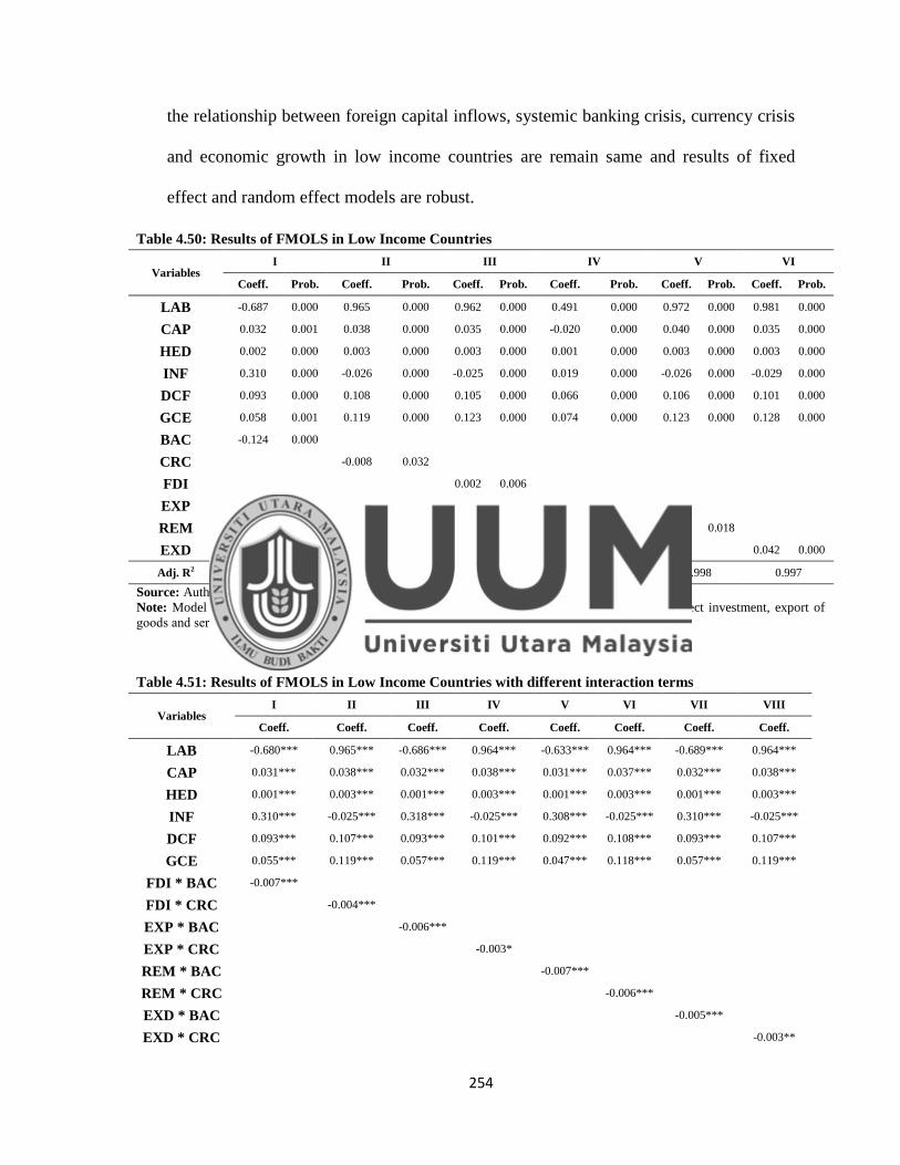
254
the relationship between foreign capital inflows, systemic banking crisis, currency crisis
and economic growth in low income countries are remain same and results of fixed
effect and random effect models are robust.
Table 4.50: Results of FMOLS in Low Income Countries
Variables I II III IV V VI
Coeff. Prob. Coeff. Prob. Coeff. Prob. Coeff. Prob. Coeff. Prob. Coeff. Prob.
LAB -0.687 0.000 0.965 0.000 0.962 0.000 0.491 0.000 0.972 0.000 0.981 0.000
CAP 0.032 0.001 0.038 0.000 0.035 0.000 -0.020 0.000 0.040 0.000 0.035 0.000
HED 0.002 0.000 0.003 0.000 0.003 0.000 0.001 0.000 0.003 0.000 0.003 0.000
INF 0.310 0.000 -0.026 0.000 -0.025 0.000 0.019 0.000 -0.026 0.000 -0.029 0.000
DCF 0.093 0.000 0.108 0.000 0.105 0.000 0.066 0.000 0.106 0.000 0.101 0.000
GCE 0.058 0.001 0.119 0.000 0.123 0.000 0.074 0.000 0.123 0.000 0.128 0.000
BAC -0.124 0.000
CRC
-0.008 0.032
FDI
0.002 0.006
EXP
0.212 0.000
REM
-0.003 0.018
EXD
0.042 0.000
Adj. R2 0.998 0.997 0.997 0.997 0.998 0.997
Source: Authors' estimation.
Note: Model I, II, III, IV, V VI represents the results of banking crises, currency crises, foreign direct investment, export of
goods and services workers‘ remittances and external debt models, respectively.
Table 4.51: Results of FMOLS in Low Income Countries with different interaction terms
Variables
I II III IV V VI VII VIII
Coeff. Coeff. Coeff. Coeff. Coeff. Coeff. Coeff. Coeff.
LAB -0.680*** 0.965*** -0.686*** 0.964*** -0.633*** 0.964*** -0.689*** 0.964***
CAP 0.031*** 0.038*** 0.032*** 0.038*** 0.031*** 0.037*** 0.032*** 0.038***
HED 0.001*** 0.003*** 0.001*** 0.003*** 0.001*** 0.003*** 0.001*** 0.003***
INF 0.310*** -0.025*** 0.318*** -0.025*** 0.308*** -0.025*** 0.310*** -0.025***
DCF 0.093*** 0.107*** 0.093*** 0.101*** 0.092*** 0.108*** 0.093*** 0.107***
GCE 0.055*** 0.119*** 0.057*** 0.119*** 0.047*** 0.118*** 0.057*** 0.119***
FDI * BAC -0.007***
FDI * CRC
-0.004***
EXP * BAC
-0.006***
EXP * CRC
-0.003*
REM * BAC
-0.007***
REM * CRC
-0.006***
EXD * BAC
-0.005***
EXD * CRC
-0.003**

255
Adj. R2 0.997 0.997 0.997 0.998 0.998 0.997 0.997 0.997
*, **, *** show significance at level of 10%, 5% and 1 % respectively
Note: Model I, II, III, IV, V, VI, VII, VIII represents the results of different interaction terms of foreign direct investment and banking crises,
foreign direct investment and currency crises, exports and banking crises, exports and currency crises, remittances and banking crises, remittances and currency crises, external debt and banking crises, external debt and currency crises,
Source: Authors' estimation.
Lower Middle Income Countries
The results of FMOLS for lower middle income countries are reported in Table 4.52 and
4.53. It is confirmed from the results of FMOLS that the coefficient of all focus variable
are having the same sign and significance after applying FMOLS. Results suggest the
negative and significant influence of banking and currency crisis on economic growth.
Results further reveal that banking and currency crisis deteriorate the positive influence
of foreign capital inflows on economic growth. Consequently, it can be concluded that
the relationship between foreign capital inflows, systemic banking crisis, currency crisis
and economic growth in lower middle income countries are remain same and results of
fixed effect and random effect models are robust.
Table 4.52: Results of FMOLS in Lower Middle Income Countries
Variables I II III IV V VI
Coeff. Prob. Coeff. Prob. Coeff. Prob. Coeff. Prob. Coeff. Prob. Coeff. Prob.
LAB 0.349 0.000 0.193 0.000 0.198 0.000 0.080 0.000 0.237 0.000 0.257 0.000
CAP 0.177 0.000 0.176 0.000 0.164 0.000 0.107 0.000 0.161 0.000 0.170 0.000
HED 0.001 0.000 0.000 0.172 0.001 0.000 0.001 0.000 0.001 0.000 0.000 0.001
INF 0.110 0.000 0.123 0.000 0.121 0.000 0.122 0.000 0.101 0.000 0.107 0.000
DCF 0.100 0.000 0.076 0.000 0.077 0.000 0.055 0.000 0.074 0.000 0.060 0.000
GCE 0.039 0.000 0.060 0.000 0.065 0.000 0.040 0.000 0.047 0.000 0.063 0.000
BAC -0.061 0.000
CRC
-0.009 0.004
FDI
0.007 0.000
EXP
0.137 0.000
REM
0.028 0.000
EXD
0.036 0.000
Adj. R2 0.997 0.997 0.998 0.998 0.997 0.997
Source: Authors' estimation.
Note: Model I, II, III, IV, V VI represents the results of banking crises, currency crises, foreign direct investment, export of
goods and services workers‘ remittances and external debt models, respectively.
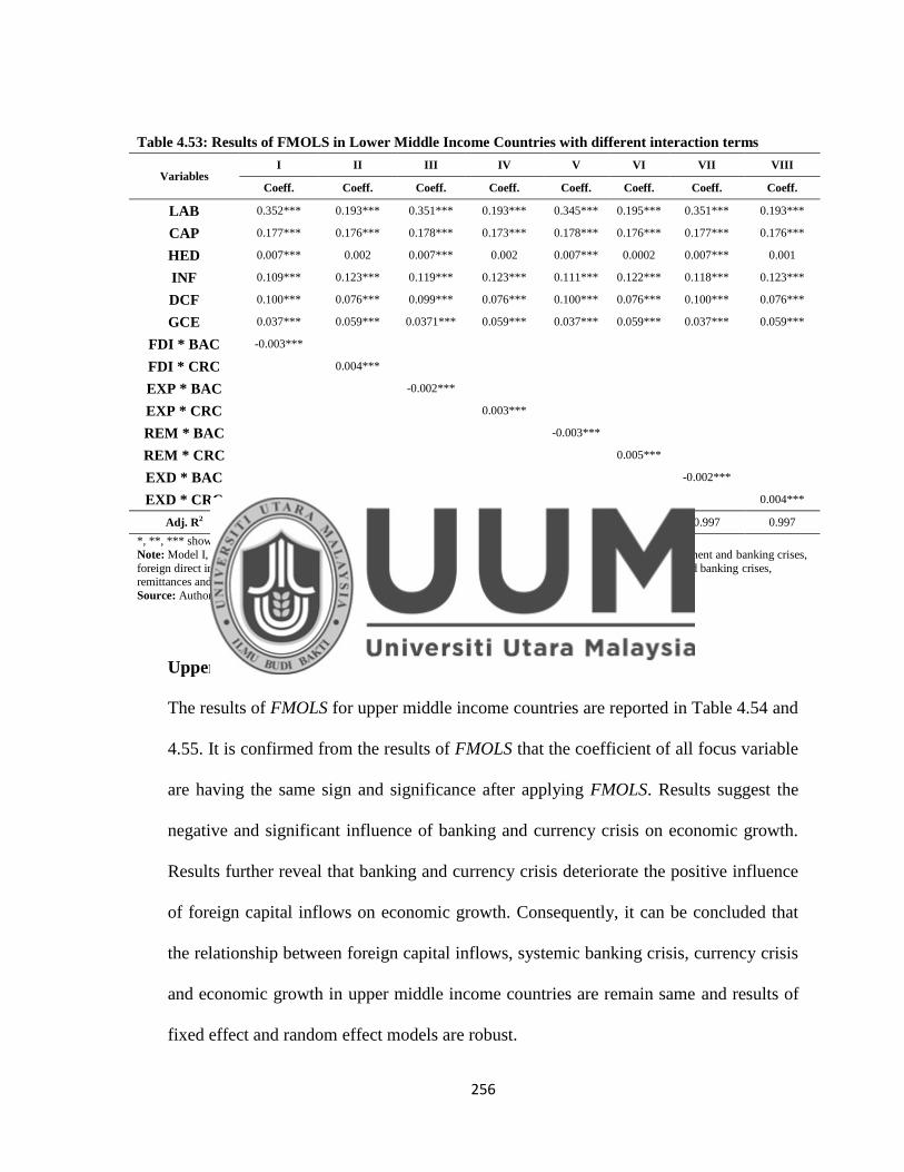
256
Table 4.53: Results of FMOLS in Lower Middle Income Countries with different interaction terms
Variables I II III IV V VI VII VIII
Coeff. Coeff. Coeff. Coeff. Coeff. Coeff. Coeff. Coeff.
LAB 0.352*** 0.193*** 0.351*** 0.193*** 0.345*** 0.195*** 0.351*** 0.193***
CAP 0.177*** 0.176*** 0.178*** 0.173*** 0.178*** 0.176*** 0.177*** 0.176***
HED 0.007*** 0.002 0.007*** 0.002 0.007*** 0.0002 0.007*** 0.001
INF 0.109*** 0.123*** 0.119*** 0.123*** 0.111*** 0.122*** 0.118*** 0.123***
DCF 0.100*** 0.076*** 0.099*** 0.076*** 0.100*** 0.076*** 0.100*** 0.076***
GCE 0.037*** 0.059*** 0.0371*** 0.059*** 0.037*** 0.059*** 0.037*** 0.059***
FDI * BAC -0.003***
FDI * CRC
0.004***
EXP * BAC
-0.002***
EXP * CRC
0.003***
REM * BAC
-0.003***
REM * CRC
0.005***
EXD * BAC
-0.002***
EXD * CRC
0.004***
Adj. R2 0.997 0.997 0.997 0.998 0.998 0.997 0.997 0.997
*, **, *** show significance at level of 10%, 5% and 1 % respectively
Note: Model I, II, III, IV, V, VI, VII, VIII represents the results of different interaction terms of foreign direct investment and banking crises,
foreign direct investment and currency crises, exports and banking crises, exports and currency crises, remittances and banking crises, remittances and currency crises, external debt and banking crises, external debt and currency crises,
Source: Authors' estimation.
Upper Middle Income Countries
The results of FMOLS for upper middle income countries are reported in Table 4.54 and
4.55. It is confirmed from the results of FMOLS that the coefficient of all focus variable
are having the same sign and significance after applying FMOLS. Results suggest the
negative and significant influence of banking and currency crisis on economic growth.
Results further reveal that banking and currency crisis deteriorate the positive influence
of foreign capital inflows on economic growth. Consequently, it can be concluded that
the relationship between foreign capital inflows, systemic banking crisis, currency crisis
and economic growth in upper middle income countries are remain same and results of
fixed effect and random effect models are robust.
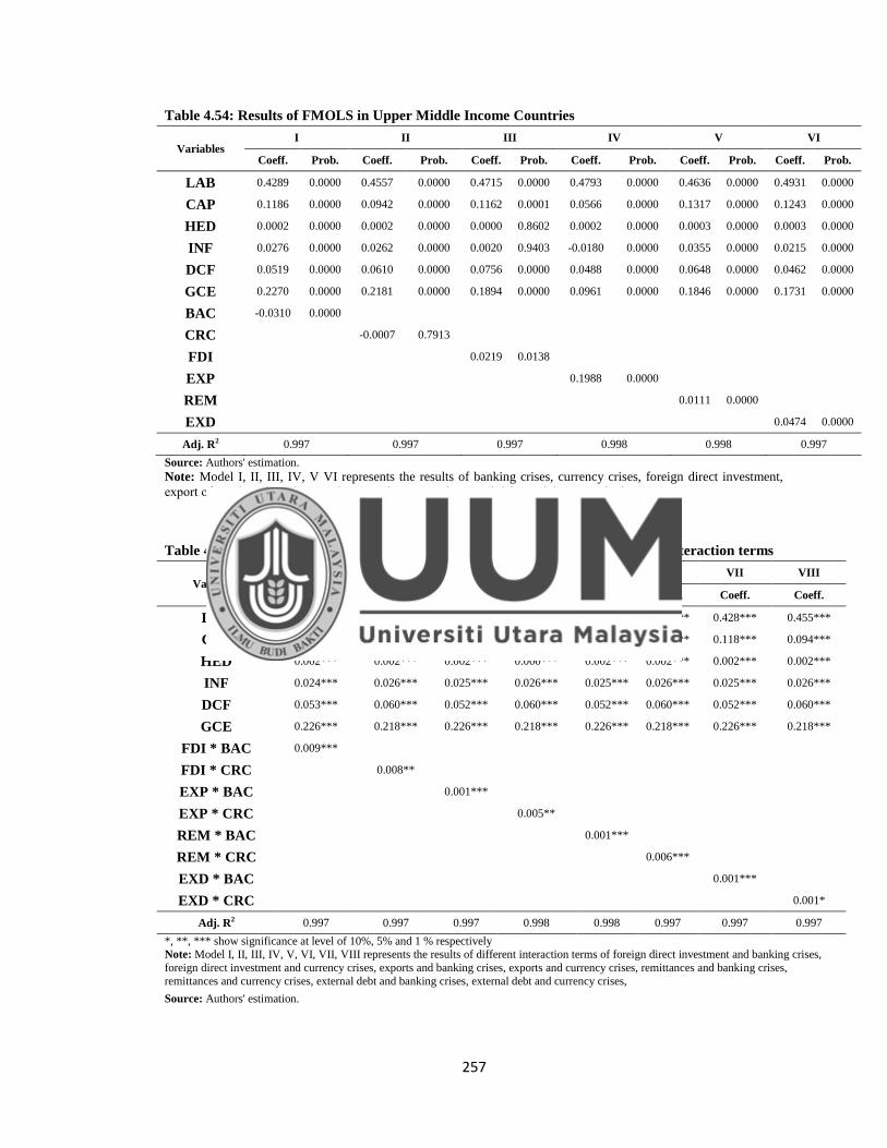
257
Table 4.54: Results of FMOLS in Upper Middle Income Countries
Variables I II III IV V VI
Coeff. Prob. Coeff. Prob. Coeff. Prob. Coeff. Prob. Coeff. Prob. Coeff. Prob.
LAB 0.4289 0.0000 0.4557 0.0000 0.4715 0.0000 0.4793 0.0000 0.4636 0.0000 0.4931 0.0000
CAP 0.1186 0.0000 0.0942 0.0000 0.1162 0.0001 0.0566 0.0000 0.1317 0.0000 0.1243 0.0000
HED 0.0002 0.0000 0.0002 0.0000 0.0000 0.8602 0.0002 0.0000 0.0003 0.0000 0.0003 0.0000
INF 0.0276 0.0000 0.0262 0.0000 0.0020 0.9403 -0.0180 0.0000 0.0355 0.0000 0.0215 0.0000
DCF 0.0519 0.0000 0.0610 0.0000 0.0756 0.0000 0.0488 0.0000 0.0648 0.0000 0.0462 0.0000
GCE 0.2270 0.0000 0.2181 0.0000 0.1894 0.0000 0.0961 0.0000 0.1846 0.0000 0.1731 0.0000
BAC -0.0310 0.0000
CRC
-0.0007 0.7913
FDI
0.0219 0.0138
EXP
0.1988 0.0000
REM
0.0111 0.0000
EXD
0.0474 0.0000
Adj. R2 0.997 0.997 0.997 0.998 0.998 0.997
Source: Authors' estimation.
Note: Model I, II, III, IV, V VI represents the results of banking crises, currency crises, foreign direct investment,
export of goods and services workers‘ remittances and external debt models, respectively.
Table 4.55: Results of FMOLS in Upper Middle Income Countries with different interaction terms
Variables I II III IV V VI VII VIII
Coeff. Coeff. Coeff. Coeff. Coeff. Coeff. Coeff. Coeff.
LAB 0.426*** 0.455*** 0.427*** 0.455*** 0.431*** 0.455*** 0.428*** 0.455***
CAP 0.117*** 0.094*** 0.117*** 0.094*** 0.118*** 0.094*** 0.118*** 0.094***
HED 0.002*** 0.002*** 0.002*** 0.000*** 0.002*** 0.002*** 0.002*** 0.002***
INF 0.024*** 0.026*** 0.025*** 0.026*** 0.025*** 0.026*** 0.025*** 0.026***
DCF 0.053*** 0.060*** 0.052*** 0.060*** 0.052*** 0.060*** 0.052*** 0.060***
GCE 0.226*** 0.218*** 0.226*** 0.218*** 0.226*** 0.218*** 0.226*** 0.218***
FDI * BAC 0.009***
FDI * CRC
0.008**
EXP * BAC
0.001***
EXP * CRC
0.005**
REM * BAC
0.001***
REM * CRC
0.006***
EXD * BAC
0.001***
EXD * CRC
0.001*
Adj. R2 0.997 0.997 0.997 0.998 0.998 0.997 0.997 0.997
*, **, *** show significance at level of 10%, 5% and 1 % respectively Note: Model I, II, III, IV, V, VI, VII, VIII represents the results of different interaction terms of foreign direct investment and banking crises,
foreign direct investment and currency crises, exports and banking crises, exports and currency crises, remittances and banking crises,
remittances and currency crises, external debt and banking crises, external debt and currency crises,
Source: Authors' estimation.
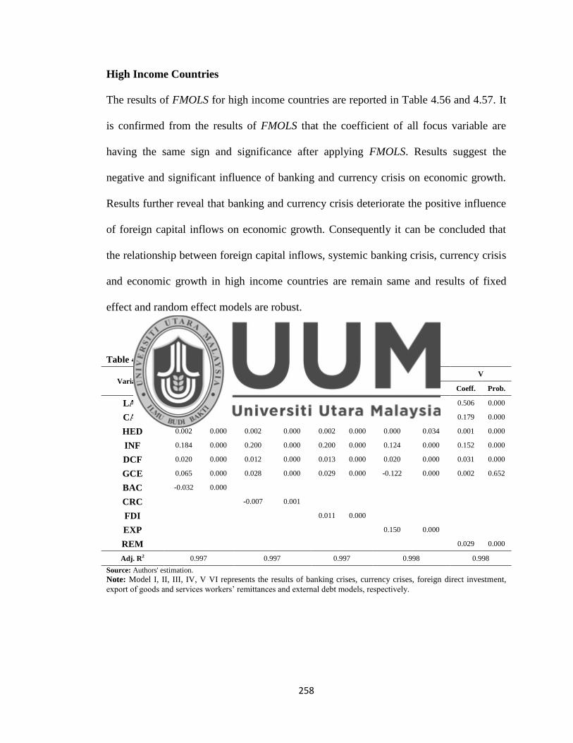
258
High Income Countries
The results of FMOLS for high income countries are reported in Table 4.56 and 4.57. It
is confirmed from the results of FMOLS that the coefficient of all focus variable are
having the same sign and significance after applying FMOLS. Results suggest the
negative and significant influence of banking and currency crisis on economic growth.
Results further reveal that banking and currency crisis deteriorate the positive influence
of foreign capital inflows on economic growth. Consequently it can be concluded that
the relationship between foreign capital inflows, systemic banking crisis, currency crisis
and economic growth in high income countries are remain same and results of fixed
effect and random effect models are robust.
Table 4.56: Results of FMOLS in High Income Countries
Variables I II III IV V
Coeff. Prob. Coeff. Prob. Coeff. Prob. Coeff. Prob. Coeff. Prob.
LAB 0.381 0.000 0.435 0.000 0.439 0.000 0.425 0.000 0.506 0.000
CAP 0.171 0.000 0.189 0.000 0.176 0.000 0.193 0.000 0.179 0.000
HED 0.002 0.000 0.002 0.000 0.002 0.000 0.000 0.034 0.001 0.000
INF 0.184 0.000 0.200 0.000 0.200 0.000 0.124 0.000 0.152 0.000
DCF 0.020 0.000 0.012 0.000 0.013 0.000 0.020 0.000 0.031 0.000
GCE 0.065 0.000 0.028 0.000 0.029 0.000 -0.122 0.000 0.002 0.652
BAC -0.032 0.000
CRC
-0.007 0.001
FDI
0.011 0.000
EXP
0.150 0.000
REM
0.029 0.000
Adj. R2 0.997 0.997 0.997 0.998 0.998
Source: Authors' estimation.
Note: Model I, II, III, IV, V VI represents the results of banking crises, currency crises, foreign direct investment,
export of goods and services workers‘ remittances and external debt models, respectively.
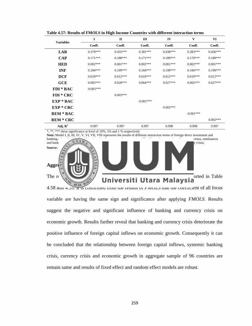
259
Table 4.57: Results of FMOLS in High Income Countries with different interaction terms
Variables I II III IV V VI
Coeff. Coeff. Coeff. Coeff. Coeff. Coeff.
LAB 0.379*** 0.435*** 0.381*** 0.436*** 0.383*** 0.436***
CAP 0.171*** 0.188*** 0.171*** 0.189*** 0.170*** 0.189***
HED 0.002*** 0.001*** 0.002*** 0.001*** 0.002*** 0.001***
INF 0.184*** 0.199*** 0.184*** 0.199*** 0.184*** 0.199***
DCF 0.019*** 0.012*** 0.019*** 0.012*** 0.019*** 0.012***
GCE 0.065*** 0.028*** 0.064*** 0.027*** 0.065*** 0.027***
FDI * BAC -0.001***
FDI * CRC
0.003***
EXP * BAC
-0.001***
EXP * CRC
0.002***
REM * BAC
-0.001***
REM * CRC
0.002***
Adj. R2 0.997 0.997 0.997 0.998 0.998 0.997
*, **, *** show significance at level of 10%, 5% and 1 % respectively Note: Model I, II, III, IV, V, VI, VII, VIII represents the results of different interaction terms of foreign direct investment and
banking crises, foreign direct investment and currency crises, exports and banking crises, exports and currency crises, remittances
and banking crises, remittances and currency crises, external debt and banking crises, external debt and currency crises,
Source: Authors' estimation.
Aggregate Sample of 96 Countries
The results of FMOLS for the aggregate sample of 96 countries are reported in Table
4.58 and 4.59. It is confirmed from the results of FMOLS that the coefficient of all focus
variable are having the same sign and significance after applying FMOLS. Results
suggest the negative and significant influence of banking and currency crisis on
economic growth. Results further reveal that banking and currency crisis deteriorate the
positive influence of foreign capital inflows on economic growth. Consequently it can
be concluded that the relationship between foreign capital inflows, systemic banking
crisis, currency crisis and economic growth in aggregate sample of 96 countries are
remain same and results of fixed effect and random effect models are robust.
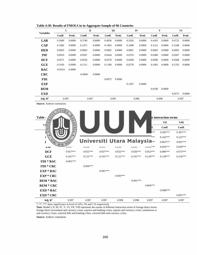
260
Table 4.58: Results of FMOLS in in Aggregate Sample of 96 Countries
Variables I II III IV V VI
Coeff. Prob. Coeff. Prob. Coeff. Prob. Coeff. Prob. Coeff. Prob. Coeff. Prob.
LAB 0.3490 0.0000 0.3740 0.0000 0.4056 0.0000 0.3503 0.0000 0.4183 0.0000 0.4725 0.0000
CAP 0.1682 0.0000 0.1471 0.0000 0.1493 0.0000 0.1098 0.0000 0.1512 0.0000 0.1248 0.0000
HED 0.0003 0.0000 0.0002 0.0000 0.0002 0.0000 0.0001 0.0000 0.0002 0.0000 0.0002 0.0000
INF 0.0919 0.0000 0.0567 0.0000 0.0434 0.0000 0.0376 0.0000 0.0386 0.0000 0.0267 0.0000
DCF 0.0571 0.0000 0.0526 0.0000 0.0570 0.0000 0.0449 0.0000 0.0586 0.0000 0.0568 0.0000
GCE 0.1010 0.0000 0.1211 0.0000 0.1180 0.0000 0.0278 0.0000 0.1065 0.0000 0.1335 0.0000
BAC -0.0314 0.0000
CRC
-0.0090 0.0000
FDI
0.0075 0.0000
EXP
0.1597 0.0000
REM
0.0169 0.0000
EXD
0.0575 0.0000
Adj. R2 0.997 0.997 0.997 0.998 0.998 0.997
Source: Authors' estimation.
Table 4.59: Results of FMOLS in in Aggregate Sample of 96 Countries with different interaction terms
Variables I II III IV V VI VII VIII
Coeff. Coeff. Coeff. Coeff. Coeff. Coeff. Coeff. Coeff.
LAB 0.352*** 0.374*** 0.350*** 0.374*** 0.347*** 0.374*** 0.392*** 0.397***
CAP 0.167*** 0.147*** 0.168*** 0.147*** 0.167*** 0.147*** 0.142*** 0.122***
HED 0.002*** 0.001*** 0.002*** 0.000*** 0.002*** 0.001*** 0.002*** 0.001***
INF 0.091*** 0.056*** 0.091*** 0.056*** 0.092*** 0.056*** 0.056*** 0.029***
DCF 0.057*** 0.052*** 0.057*** 0.052*** 0.056*** 0.052*** 0.080*** 0.073***
GCE 0.101*** 0.121*** 0.101*** 0.121*** 0.101*** 0.120*** 0.138*** 0.154***
FDI * BAC -0.001***
FDI * CRC
0.004***
EXP * BAC
-0.001***
EXP * CRC
0.003***
REM * BAC
-0.001***
REM * CRC
0.004***
EXD * BAC
-0.008***
EXD * CRC
0.001***
Adj. R2 0.997 0.997 0.997 0.998 0.998 0.997 0.997 0.997
*, **, *** show significance at level of 10%, 5% and 1 % respectively
Note: Model I, II, III, IV, V, VI, VII, VIII represents the results of different interaction terms of foreign direct investment and banking crises,
foreign direct investment and currency crises, exports and banking crises, exports and currency crises, remittances and banking crises, remittances
and currency crises, external debt and banking crises, external debt and currency crises, Source: Authors' estimation.
261
4.9 Discussion of Result
In this section, we discuss the theoretical and conceptual underpinning of earlier
presented results of different income level countries. The short summary of earlier
presented results is reported in Table 4.60. Results indicate the negative and significant
influence of systemic banking crisis in LI, LMI, UMI, HI and aggregate samples of 96
countries. This suggests that banking crisis leads to decline in the growth of an
economy. It is concluded that the banking crisis most affects the low income countries
whereas high income countries least affect by the banking crisis. Previously, empirical
studies also report that the impact of banking crisis mainly decreases the growth of an
economy (Lindgren, Garcia, and Saal (1996); Chor & Manova, 2012; Iacovone &
Zavacka, 2009). These studies conclude that the economies which are heavily dependent
on external financing, produce the worst performance in financial distress period. In the
period of financial crisis, the production and income of an economy are lower down.
The banking crisis leads to generate the negative sentiments among foreign investors
about future economic growth during (Bogach & Noy, 2012; Dornean et al., 2012;
Skovgaard Poulsen & Hufbauer, 2011).
Results further indicate the negative and significant influence of currency crises in LI,
LMI, UMI, HI and aggregate sample of 96 countries. This suggests that a currency crisis
leads to decline in the growth of an economy. It is also concluded that the currency
crisis most affects the upper middle income countries whereas, low income countries
least affect by currency crisis. A currency crisis is considered a sudden loss in
confidence and consequent depreciation of the national currency in relation to other
currencies. Furthermore, the drop in exchange rates during the financial crisis worse the

262
economic conditions and it is prolonged as long as government continues to monetize its
deficit.
Table 4.60: Summary of Estimation Results of all Countries
Low
Income
Lower
Middle
Income
Upper
Middle
Income
High
Income
Complete
Sample
BAC Coefficient -0.1048 -0.0366 -0.0399 -0.0241 -0.0237
Prob. Value 0.0626 0.0024 0.0045 0.0004 0.0002
CRC Coefficient -0.0034 -0.0252 -0.0408 -0.0128 -0.0244
Prob. Value 0.0050 0.0031 0.0001 0.0284 0.0000
FDI Coefficient 0.0071 0.0071 0.0112 0.0066 0.0059
Prob. Value 0.2279 0.0591 0.0498 0.0114 0.0083
FDI*BAC Coefficient -0.0068 -0.0020 0.0017 -0.0011 -0.0012
Prob. Value 0.0501 0.0010 0.0109 0.0003 0.0001
FDI*CRC Coefficient -0.0039 0.0010 0.0018 0.0006 0.0012
Prob. Value 0.6732 0.0182 0.0005 0.0244 0.0000
EXP Coefficient 0.2658 0.1044 0.1919 0.1300 0.1563
Prob. Value 0.0000 0.0000 0.0000 0.0000 0.0000
EXP*BAC Coefficient -0.0049 -0.0017 0.0015 -0.0010 -0.0010
Prob. Value 0.0770 0.0013 0.0084 0.0002 0.0001
EXP*CRC Coefficient 0.0015 0.0011 0.0016 0.0005 0.0010
Prob. Value 0.7965 0.0038 0.0004 0.0299 0.0000
REM Coefficient -0.0075 0.0127 0.0327 0.0194 0.0092
Prob. Value 0.3401 0.0049 0.0456 0.0000 0.0001
REM*BAC Coefficient -0.0078 -0.0017 0.0019 -0.0013 -0.0012
Prob. Value 0.0251 0.0061 0.0057 0.0001 0.0001
REM*CRC Coefficient -0.0038 0.0008 0.0018 0.0006 0.0012
Prob. Value 0.6962 0.0425 0.0007 0.0409 0.0000
EXD Coefficient 0.0715 -0.0468 0.0419
0.0348
Prob. Value 0.0029 0.0000 0.0001
0.0000
EXD*BAC Coefficient -0.0048 0.0034 0.0016
-0.0011
Prob. Value 0.0573 0.0835 0.0054
0.7945
EXD*CRC Coefficient -0.0004 -0.0044 0.0017
0.0011
Prob. Value 0.6428 0.0084 0.0002 0.0002
Results conclude the positive influence of FDI on economic growth in all income level
countries. The FDI has the highest positive impact in upper middle income countries,
these are the most emerging economies and has the highest inflows of foreign direct

263
investment. These results are consistent with the past empirical studies (Campos &
Kinoshita, 2002; Nicolini & Resmini, 2010; Siddique et al., 2012) Foreign direct
investment are perceived as a factor of economic growth, a complement to domestic
investment and a source of financing of the current account deficit. FDI contributes the
host country in the form of technological externalities, the formation of human capital or
have access to foreign markets which lead to long-term economic growth. FDI also
resulted a reduction in unemployment by creating more employment opportunities in
host economy.
In the case of FDI, the results confirm that the impact of foreign direct investment on
economic growth becomes negative and significant in the presence of systemic banking
crises in LI, LMI and HI countries whereas, the relationship remains positive and
significant in the UMI however, the magnitude of the relationship is drop down. Results
also confirm the impact of foreign direct investment on economic growth remain
positive and significant in the presence of currency crises. However, the magnitude of
relationship is significantly drop down in all income level countries. These findings
conclude that the banking and currency crisis are harmful for the relationship of foreign
direct investment and economic growth in all income level countries.
In the period of financial crisis, entrance of foreign companies in the imperfect
competitive markets may leads to reduce market share of domestic producers.
Capabilities of economies of scale also suffer in domestic producers because of loss of
market share, which also have a negative impact on productivity. The introduction of
264
new technologies assumes or requires the existence of skilled labor in the host country,
which are capable and trained on using those technologies. If the supply of labor is
shorter in the host country than it leads to a negative impact on production and
economic growth.
Results conclude the positive influence of exports of goods and services on economic
growth in all income level countries. The findings are consistent with (Balaguer &
Cantavella-Jorda, 2002; Dodaro, 1991; Omri, Daly, Rault, & Chaibi, 2015; Tang, Lai, &
Ozturk, 2015; Vamvoukas, 2007). The export has the highest positive impact in low
income countries followed by upper middle income countries. The spillover effect of the
export sector in the production process of an economy contributes in the total
productivity of a country. Moreover, export help in importing high value technology
products and inputs that cause increases in the productive capacity of a country which
also leads to improve the efficiency in the production process. The realization of
economies of scale results exports rises with the help of rise in productivity. This
increment in exports can further reduce cost, which may also increase in the productivity
growth.
In the case of exports of goods and services, the results confirm that the impact of
exports of goods and services on economic growth becomes negative and significant in
the presence of systemic banking crises in LI, LMI and HI countries whereas, the
relationship remains positive and significant in the UMI however, the magnitude of
relationship is dropped down. Results also confirm the impact of exports on economic

265
growth remain positive and significant in the presence of currency crises. However, the
magnitude of relationship is significantly drop down in all income level countries. These
findings conclude that the banking and currency crisis are harmful for the relationship of
exports of goods and services and economic growth in all income level countries. The
possibility of a negative linkage between economic growth and exchange rate may exist,
meaning that, rise in economic output level decline in the export growth level. On the
same note, the decrease in economic growth in the presence of export growth occurs
when growth in exports is appreciating against the domestic consumption.
Results also conclude the positive influence of workers‘ remittances on economic
growth in all income level countries. The remittances have the highest positive impact in
upper middle income countries. The findings are consistent with (N Catrinescu & Leon,
2010; Faini, 2007; Ramirez & Sharma, 2008; World Bank, 2006b; Ziesemer, 2006;
Cooray, 2012; Nsiah and Fayissa, 2013; Jawaid and Raza, 2014; Goschin, 2014; M. Al
Mamun, Sohag, Uddin, and Shahbaz, 2015; Oshota and Badejo, 2015). Workers‘
remittances have been proved to be a source of alleviating poverty in developing
countries. The increase in workers‘ remittances also resulted in an increase in the private
investments. Furthermore, remittances are found to be in a positive trend when the host
economy suffers a recession because of financial crisis, political conflicts or natural
disasters, etc. as expatriates remit more during a crucial time for so that they can support
their families and nations accordingly.
266
In the case of workers‘ remittances, the results confirm that the impact of remittances on
economic growth becomes negative and significant in the presence of systemic banking
crises in LI, LMI and HI countries whereas, the relationship remains positive and
significant in the UMI however, the magnitude of the relationship is drop down. Results
also confirm the impact of remittances on economic growth remain positive and
significant in the presence of currency crises. However, the magnitude of relationship is
significantly drop down in all income level countries. These findings conclude that the
banking and currency crisis are harmful for the relationship of remittances and economic
growth in all income level countries. The economic growth may have a negative impact
of remittances in the host country which causes the decrease in labor force participation.
This type of capital inflows may consider just as transfer of income. Furthermore, this
transfer of income may be stressed by the severe moral hazard problem. In this regard,
the recipients promotes to use alternate way of consumption and the labor market effort
reduce accordingly. The migrant‘s remittances may not be considered as profit driven
due to spending on consumption rather than on investment activities. The imports may
increase through remittances in the country which further widen the deficit in balance of
payment.
Furthermore, the another reason behind this negative association is when the migration
increases in the country, it increases the dependency on remittance. This dependence on
remittance increases the income inequality in the region, which hinders the economic
development. The high remittance inflow results in an appreciation of the exchange rate,
which affects the sectorial production, especially the trade sector which slow down the
267
economic growth. Furthermore, the emigrants that usually go aboard are highly
educated and skilled which causes the brain drain within the economy and reduces the
economic development, because home country invested the money, effort and time in
their education. The negative relationship is also consistent with the past empirical
literature of Chami et al. (2003), Chami, Cosimano, and Gapen (2006), Amuedo-
Dorantes & Pozo, 2004; Lartey, Mandelman, & Acosta, 2008; Lopez, Bussolo, &
Molina, 2007, Jawaid and Raza (2014), Kumar (2014), Oshota and Badejo (2015),
Jouini (2015).
Results also conclude the positive influence of foreign debt on economic growth in all
income level countries. The foreign debt has the highest positive impact in low income
countries followed by lower middle income countries. The findings are consistent with
D. Cohen (1991); Çiçek, Gözegir, and Çevik (2010); Bakar and Hassan (2011); Umutlu,
Alizadeh, and Erkılıç (2011); Kasidi and Said (2013); Daud et al. (2013); Wahiba
(2014); Fincke and Greiner (2015). The countries borrow for two broad reasons;
macroeconomic reason that is to finance higher levels of consumption and investment or
to finance the transitory balance of payment deficit and avoid budget constraint so as to
boost economic growth and reduce poverty. External debt is a major source of public
receipts and financing capital accumulation in any economy. It is a medium used by
countries to bridge their deficits and carry out economic projects that are able to increase
the standard of living of the citizenry and promote sustainable growth and development.
268
In the case of foreign debt, the results confirm that the impact of foreign debt on
economic growth becomes negative and significant in the presence of systemic banking
crises in LI countries whereas, the relationship remains positive and significant in the
LMI and UMI however, the magnitude of the relationship is drop down. Results also
confirm the impact of foreign debt on economic growth becomes negative and
significant in the presence of systemic banking crises in LI and LMI countries whereas,
the relationship remains positive and significant in the UMI countries however, the
magnitude of the relationship is drop down. These findings conclude that the banking
and currency crisis are harmful for the relationship of external debt and economic
growth in all income level countries. Debt service payments create a lot of problems for
countries, especially the developing nation's reason being that a debt is actually serviced
for more than the amount it was acquired and this slows down the growth process in
such nations. Daud, Ahmad, and Azman-Saini (2013) asserted that at low levels debt has
positive effects on growth but above particular points or thresholds accumulated debt
begins to have a negative impact on growth. Furthermore, the high debt service
payments shift spending away from health, educational and other social sectors.
4.10 Summary of Chapter
In this chapter, we present the results of empirical estimations and further discuss these
results in the theoretical and conceptual context. Results of unit root estimation prove
that there is no problem of unit root in our considered variables and we can further use
these variables for the long run estimations. Results of Pedroni and Kao cointegration
method indicate the rejection of null hypothesis of no cointegration in the favor of valid
269
long run cointegration for the all income level countries. Results of long run analysis
indicate the negative and significant influence of systemic banking and currency crisis in
LI, LMI, UMI and HI countries. These findings conclude that the systemic banking
crisis and currency crisis are harmful for the economic growth for all income level
countries. It is concluded that the banking crisis most affects the low income countries
whereas high income countries least affect by the banking crisis. Furthermore, it is also
concluded that the currency crisis most affects the upper middle income countries
whereas, low income countries least affect by currency crisis. Results also indicate the
positive and significant impact of all four types of FCI on economic growth in all
income level countries except, remittances in low income countries and foreign debt in
lower middle income. These two results show the negative impact on economic growth.
These findings conclude that the banking and currency crisis are harmful for the
relationship of foreign capital inflows and economic growth in all income level
countries.

270
CHAPTER FIVE
SUMMARY OF MAJOR FINDINGS, CONCLUSION AND POLICY
IMPLICATIONS
5.1 Introduction
The chapter presents summary of major findings, conclusion, policy implication and
recommendation for future study. In the summary and conclusion section, we briefly
discuss the need, objective, contribution, sample size and results of this study. Similarly,
the policy implication and limitation of the study are also presented. Recommendation
for future research and conclusion are equally made.
5.2 Summary of Major Findings & Conclusion
Foreign capital inflows play a significant role in the economic growth of both
developing and developed countries. Foreign capital has also been considered to be a
key element in the process of economic globalization and integration of the world
economy. The flows of capital have been welcomed, to complement domestic financial
resources, as a development catalyst. The resource deficient economies relied heavily on
foreign capital to achieve the objective of higher economic growth. In the last two
decades, the frequent occurrence of financial crises around the world, has awakened the
debate about the causes, consequences, impact and aftershocks of these crises. These
sorts of financial crises are majorly occurring because of systemic banking crisis and
currency crisis. These crises significantly influence the relationship between FCI and
economic growth. There are very few studies have been done which analyze the impact
of financial crisis on the FCI. The movement of FCI is a matter of different income level
271
countries and it is generally moved from high and upper middle income countries to
lower middle and low income countries.
The objective of this study is to identify the impact of foreign direct investment, foreign
debt, workers‘ remittances and exports of goods and services on economic growth in
high, upper middle, lower middle and low income countries. Furthermore, the more
unique contribution of this study to analyze the impact of foreign capital inflows on
economic growth of different income level countries in the presence of currency and
banking crises. To attain the objective of this research we collect the panel data of 96
countries and group them on the basis of different income levels. The final sample of
this study consists of 10 low income countries, 23 lower middle income countries, 30
upper middle income countries and 33 high income countries. We employed fixed effect
& random effect model to judge the desired relationship among variables. Fully
modified ordinary least squares (FMOLS) has also been used to ensure the robustness of
initial results.
Results indicate the negative and significant influence of systemic banking and currency
crisis in LI, LMI, UMI and HI countries. These findings conclude that the systemic
banking crisis and currency crisis are harmful for the economic growth for all income
level countries. It is concluded that the banking crisis most affects the low income
countries whereas high income countries least affect by the banking crisis. Furthermore,
it is also concluded that the currency crisis most affects the upper middle income
countries whereas, low income countries least affect by currency crisis. Results also

272
indicate the positive and significant impact of all four types of FCI on economic growth
in all income level countries except, remittances in low income countries and foreign
debt in lower middle income. These two results show the negative impact on economic
growth.
In the case of FDI, the results confirm that the impact of foreign direct investment on
economic growth becomes negative and significant in the presence of systemic banking
crises in LI, LMI and HI countries whereas, the relationship remains positive and
significant in the UMI however, the magnitude of the relationship is drop down. Results
also confirm the impact of foreign direct investment on economic growth remain
positive and significant in the presence of currency crises. However, the magnitude of
relationship is significantly drop down in all income level countries. These findings
conclude that the banking and currency crisis are harmful for the relationship of foreign
direct investment and economic growth in all income level countries.
In the case of exports of goods and services, the results confirm that the impact of
exports of goods and services for economic growth becomes negative and significant in
the presence of systemic banking crises in LI, LMI and HI countries whereas, the
relationship remains positive and significant in the UMI however, the magnitude of the
relationship is drop down. Results also confirm the impact of exports on economic
growth remain positive and significant in the presence of currency crises. However, the
magnitude of relationship is significantly drop down in all income level countries. These

273
findings conclude that the banking and currency crisis are harmful for the relationship of
exports of goods and services and economic growth in all income level countries.
In the case of workers‘ remittances, the results confirm that the impact of remittances on
economic growth becomes negative and significant in the presence of systemic banking
crises in LI, LMI and HI countries whereas, the relationship remains positive and
significant in the UMI however, the magnitude of the relationship is drop down. Results
also confirm the impact of remittances on economic growth remain positive and
significant in the presence of currency crises. However, the magnitude of relationship is
significantly drop down in all income level countries. These findings conclude that the
banking and currency crisis are harmful for the relationship of remittances and economic
growth in all income level countries.
In the case of foreign debt, the results confirm that the impact of foreign debt on
economic growth becomes negative and significant in the presence of systemic banking
crises in LI countries whereas, the relationship remains positive and significant in the
LMI and UMI however, the magnitude of the relationship is drop down. Results also
confirm the impact of foreign debt on economic growth becomes negative and
significant in the presence of systemic banking crises in LI and LMI countries whereas,
the relationship remains positive and significant in the UMI countries however, the
magnitude of the relationship is drop down. These findings conclude that the banking
and currency crisis are harmful for the relationship of external debt and economic
growth in all income level countries.
274
5.3 Policy Implications
Having established that all four types of foreign capital inflows are positively associated
with economic growth and systemic banking crisis and currency are negatively
associated with economic growth in all income level countries. Furthermore, the
findings conclude that the banking and currency crisis are harmful for the relationship of
FCI and economic growth in all income level countries. We recommend the following
policy implications:
The results suggest that the exports of the country have significant positive impact on
economic growth. Moreover, the banking and systemic crisis hurt the relationship
between EXP and EG. It is recommended that the country can improve the economic
growth at the time of financial crisis by diversifying their trade in terms of products and
partners, both. They should implement the expansionary monetary policies and should
have multilateral organizations that provide them funding at the time of economic
shocks. In addition to this, to avert the financial crisis in the future, the economy should
focus on achieving the optimal macro-economic policies. The foremost important policy
is to improve the financial and trade integration. This can be done by signing the
bilateral trade contracts, bilateral free trade contracts with the rest of the countries in the
world. Moreover, the trade integration should also be encouraged at the provincial level
as this will strengthen the local markets. The improved financial integration increases
the economy attractiveness and results in FDI inflows.
The main problem for any economy is, in what manner the export should be improved
which would result in the growth expansion. From the policy view, the economies

275
should focus on liberal trade policies in order to make strong relationships with other
economies. Along with that, the country should also focus on efficient production of the
domestic industries because the maximum benefit from exports can only be gained if the
industries perform well. The industries that do not perform well should be eliminated by
using the one-sided trade liberalization measures as this will help to minimize the trade
risks.
The country should also focus on technological improvement to match the international
quality requirement and to meet the high export goals. The investment on supply-side
policies such as education and infrastructure should also be encouraged as they have the
direct impact on exports. Moreover, the stable exchange rate policies should also be
implemented because stable prices help the export expansion. Another way in which the
export can be improved is allocation of resources on the basis of comparative advantage
and achieving economies of scale because this lowers down the cost of export goods and
make it more competitive in other economies, thus, enhancing the economic growth.
The results suggest that the FDI inflow of the country has significant positive impact on
economic growth. Moreover, the banking and systemic crisis hurt the relationship
between FDI and EG. It is recommended that at the time of crisis, government should
play the role to minimize the negative impact of crisis by acting as a stabilizer for the
foreign investors. The multinational corporations (MNCs) work in both countries (home
and host) so they share the economic shocks. The FDI can be encouraged in the
economy by introducing the financial reforms and improving the domestic financial

276
sector. The country‘s domestic performance should be emphasized because this not only
improves the MNC performance, but it will also allow the economy to enjoy the
maximum benefits from FDI inflows.
The policy makers should encourage the FDI by establishing those policies that improve
the local firm access to technology, finance, inputs, encourages them to establish
linkages. Moreover, the country should attract more FDI by giving attractive fiscal
incentives and protected environment in order to generate income, employment and
enhance economic growth. The countries should relax the regularity restrictions on
capital flows in order to enjoy the benefit from capital inflows. Economic policies that
stimulate the capital flows should be implemented as they increase the FDI effect on
economic growth. To enjoy the positive effect of FDI on economic growth the economy
should focus on a sustainable FDI strategy which focuses on quality and quantity both.
They should implement those policies the boost human capital and infrastructure
development as they both influence economic growth in an effective manner.
The results suggest that the flow of workers‘ remittances in the country has significant
positive impact on economic growth. Moreover, the banking and systemic crisis hurt the
relationship between REM and EG. Worker remittances are considered as a boon to the
countries. It has a positive association with the economic growth and acts a stabilizer
during the financial crisis. To ensure the effective inflows of the remittance the
government should encourage that remittance should be transferred through formal
channels, this can be done by giving cost effective financial services to the remitter,
277
linking the remittance transfer with mobile networks and banks that charge low prices.
The remittance transfer through formal channels increases the foreign currency reserves
and at the time of financial crisis, these reserves can be used to maintain the
macroeconomic stability, to minimize the effect of negative shocks and help to boost the
economic growth. Moreover, during the financial crisis, it also lessens credit constraints
faced by the country.
The government authorities should also use the remittance inflows in a productive
manner which results in creating employment opportunities. For this, the government
should encourage tax exempted projects, establish new business in different sectors, and
give incentives on investment, as this will encourage the remitter to invest the money
and results in increased remittance inflows. Moreover, the authorities should develop
policies that encourage international migration and use the remittances in promoting
domestic production.
During the financial crisis, the remittance acts as a cushion in minimizing the worst
effects. To maintain the economic growth at the financial crisis the economies should
involve in global integration as it is one of the beneficial path to follow. The countries
should also consider the wealth of the overseas diaspora as one of the potential sources
of capital and it should be increased by issuing financial instruments such as diaspora
bonds as this is one of the sources through which the remittances can be secure for the
future.

278
The results suggest that the flow of foreign debt in the country has significant positive
impact on economic growth. Moreover, the banking and systemic crisis hurt the
relationship between EXD and EG. Countries adopt an external financing to ensure the
sustainable economic growth as domestic saving alone is not sufficient for the
development. So, the policy makers and the governments should be aware with the
importance of the effective debt management and its role in the enhancement of growth.
The authorities should use the efficient techniques in the acquisition and deployment of
the debt. They should closely monitor the application of the external borrowing and
confirms that they are used in an efficient and effective manner. The continuous
monitoring should be done to affirm that the optimal debt does not exceed the
benchmark. Furthermore, when the government faces the debt, deficit and plan to go for
external borrowing they should do an analysis and ensure that this borrowing will not
result in debt overhang.
If the countries found the overhang situation the government prior focus should be its
reduction. It can be done through debt rescheduling, debt buy backs, debt restructuring
or write-off. This will also help the countries to maintain the internationally accepted
debt ratio level, i.e., 45% of GDP. The government should make those fiscal policies
which endorses debt sustainability because debt is helpful for the growth of the
economy if does not exceed the optimum level. Moreover, the government expenditure
should also be reduced as this improve the debt situation.

279
The excessive dependency on external debt brings in negative results so the effective
external debt management and maintaining optimum level is of key importance.
To achieve this, the external borrowing should be used in the industrial sector of the
economies because it directly increases the production and ultimately results in the
economic growth. Moreover, the organizations should use the external debt in export
oriented areas and in the encouragement of financial, trade, since during the financial
crisis, the diversification in financial trade helps to generate the export proceed which is
the prime source in the repayment of external debts. It is recommended to the
governments that during the financial crisis, they should focus on the debt
transformation rates in order to promote economic growth by means of foreign capital.
The foreign exchange reserve is of crucial importance in order to pay external
borrowing so the good relationship with the investors should be encouraged by
promoting trade openness and trade liberalization. Moreover, the government should
ensure political stability in order to gain the confidence of both local and foreign
investors. This will help the countries to reduce their reliance on external debt. The
stable environment also increases the Foreign Direct Investment (FDI) inflows and
through FDI the external borrowing can be minimized. So, the policy makers should
establish those policies that encourage FDI.
5.4 Limitations of the Study
This study focuses primarily on the impact of foreign capital inflows on economic
growth and influence of systemic banking crisis and currency crisis on the relationship
280
of foreign capital inflows and economic growth in different income level countries. The
major issue we faced is about the non-availability of historical data. This study provides
the several contributions to the existing literature, whereas, still some limitations exist in
this study. We use four different flows of FCI i.e., exports, foreign debt, remittances and
FDI. However, the variables of foreign portfolio investment and grants are not used in
this study because of non-availability of enough data for all income level countries. The
study was limited to the period due to the availability of data on our variables of interest.
The sample size of our study is relatively limited from 1995 to 2013, only 14 annual
observations for each cross section. Furthermore, we only consider those countries
which have the proper data of all types of foreign capital inflows to ensure the
homogeneity of sample and results. Other than having data for only a few years there
were missing data for certain countries.
In this research, we only focus on the relationship of different income level countries.
The future researches may be conducted on the sample of different regions, like Asia,
Africa and Europe. The future researches may also be conducted on the comparative
basis between the regions. The future researches should be focused on the time series
analysis on the cases of specific country which discuss more specific results and
discussion of the separate country. The non-availability of enough literature on the topic
of influence of systemic banking and currency crisis in the relationship and economic
growth is also a limitation of this study.

281
5.5 Recommendations for Future Research
Given the limitations of the present study, we recommend that future research should
consider the issues highlighted in this section. In this research, we only focus on the
relationship of different income level countries. The future researches may be conducted
on the sample of different regions, like Asia, Africa and Europe. The future researches
may also be conducted on the comparative basis between the regions. The future
researchers may also conduct research on the basis of different other homogenous
groups, i.e. developed economies, developing economies, emerging economies, G-7
countries, BRICS countries. The future researches should be focused on the time series
analysis on the cases of specific country which discuss more specific results and
discussion of the separate country.
Furthermore, this study is based on only revenue generation based foreign capital
inflows i.e., exports, foreign debt, remittances and FDI. The future researches may be
conducted on those foreign capital inflows which come into the country to provide
support i.e. international government grants and foreign aid. Future researches may be
conducted on the disaggregate level or a sectorial basis of FDI and export in an
economy.
282
REFERENCES
A. Giles, J., & Williams, C. L. (2000). Export-led growth: a survey of the empirical
literature and some non-causality results. Part 1. Journal of International Trade
& Economic Development, 9(3), 261-337.
Abual-Foul, B. (2004). Testing the export-led growth hypothesis: evidence from Jordan.
Applied Economics Letters, 11(6), 393-396.
Acaravci, A., & Ozturk, I. (2012). Foreign direct investment, export and economic
growth: empirical evidence from new EU countries. Romanian Journal of
Economic Forecasting, 15(2), 52-67.
Achchuthan, S. (2013). Export, Import and Economic Growth: Evidence from Sri
Lanka. Journal of Economics and Sustainable Development, 4(9), 147-155.
Adam, C. S., & Bevan, D. L. (2005). Fiscal deficits and growth in developing countries.
Journal of Public Economics, 89(4), 571-597.
Adams, R. H. (2009). The determinants of international remittances in developing
countries. World Development, 37(1), 93-103.
Adams Richard, H., & Page, J. (2003). International Migration, Remittances and
Poverty in Developing Countries. World Bank Policy Research Working Paper,
3179.
Adelman, I., & Taylor, J. E. (1990). Is structural adjustment with a human face
possible? The case of Mexico. The Journal of Development Studies, 26(3), 387-
407.
283
Adeniyi, O., Omisakin, O., Egwaikhide, F. O., & Oyinlola, A. (2012). Foreign direct
investment, economic growth and financial sector development in small open
developing economies. Economic Analysis and Policy, 42(1), 105-127.
Adepoju, A. A., Salau, A. S., & Obayelu, A. E. (2007). The effects of external debt
management on sustainable economic growth and development: lessons from
Nigeria.
Aditya, A., & Acharyya, R. (2013). Export diversification, composition, and economic
growth: Evidence from cross-country analysis. The Journal of International
Trade & Economic Development, 22(7), 959-992.
Agrawal, G., & Khan, M. (2011). Impact of FDI on GDP growth: A panel data study.
European Journal of Scientific Research, 57(2), 257-264.
Ahmad, J., & Harnhirun, S. (1996). Cointegration and causality between exports and
economic growth: evidence from the ASEAN countries. Canadian Journal of
Economics, S413-S416.
Ahmed, A. D., Cheng, E., & Messinis, G. (2007). Causal links between export, FDI and
output: Evidence from sub-Saharan African countries.
Ahmed, H. A., & Uddin, M. G. S. (2009). Export, imports, remittance and growth in
Bangladesh: An empirical analysis. Trade and Development Review, 2(2).
Ahrend, R., Arnold, J. M., & Murtin, F. (2011). Have more strictly regulated banking
systems fared better during the recent financial crisis? Applied Economics
Letters, 18(5), 399-403.
Aitymbetov, S. (2006). Emigrant remittances: Impact on economic development of
kyrgyzstan. Kyrgyzstan, The Economic Policy Institute.
284
Ajmi, A. N., Aye, G. C., Balcilar, M., & Gupta, R. (2015). Causality between exports
and economic growth in South Africa: Evidence from linear and nonlinear tests.
The Journal of Developing Areas, 49(2), 163-181.
Akerlof, G. A., Romer, P. M., Hall, R. E., & Mankiw, N. G. (1993). Looting: the
economic underworld of bankruptcy for profit. Brookings Papers on Economic
Activity, 1-73.
Akinlo, A. E. (2004). Foreign direct investment and growth in Nigeria: An empirical
investigation. Journal of Policy Modeling, 26(5), 627-639.
Akram, N. (2015). Is public debt hindering economic growth of the Philippines?
International Journal of Social Economics, 42(3), 202-221.
Al-Iriani, M. (2007). Foreign direct investment and economic growth in the GCC
countries: A causality investigation using heterogeneous panel analysis.
Al Mamun, K. A., & Nath*, H. K. (2005). Export-led growth in Bangladesh: a time
series analysis. Applied Economics Letters, 12(6), 361-364.
Al Mamun, M., Sohag, K., Uddin, G. S., & Shahbaz, M. (2015). Remittance and
domestic labor productivity: evidence from remittance recipient countries.
Economic Modelling, 47, 207-218.
Alfaro, L., Chanda, A., Kalemli-Ozcan, S., & Sayek, S. (2004). FDI and economic
growth: the role of local financial markets. Journal of international economics,
64(1), 89-112.
Alfaro, L., Chanda, A., Kalemli-Ozcan, S., & Sayek, S. (2010). Does foreign direct
investment promote growth? Exploring the role of financial markets on linkages.
Journal of Development Economics, 91(2), 242-256.
285
Alfaro, L., Rodríguez-Clare, A., Hanson, G. H., & Bravo-Ortega, C. (2004).
Multinationals and linkages: An empirical investigation [with comments].
Economia, 113-169.
Ali, S. (2014). Foreign capital flows and economic growth in Pakistan: An empirical
analysis. Ali, Sharafat (2014). Foreign Capital Flows and Economic Growth in
Pakistan: An Empirical Analysis. World Applied Sciences Journal, 29(2), 193-
201.
Alleyne, D., Kirton, C. D., & Figueroa, M. (2008). Macroeconomic determinants of
migrant remittances to Caribbean Countries: Panel Unit roots and cointegration.
The Journal of Developing Areas, 137-153.
Aluko, F., & Arowolo, D. (2010). Foreign aid, the Third World‘s debt crisis and the
implication for economic development: The Nigerian experience. African
Journal of Political Science and International Relations, 4(4), 120-127.
Amuedo-Dorantes, C., & Pozo, S. (2004). Workers' remittances and the real exchange
rate: a paradox of gifts. World Development, 32(8), 1407-1417.
Andini, C., & Cabral, R. (2012). Further austerity and wage cuts will worsen the euro
crisis: IZA Policy Paper.
Andraz, J. M., & Rodrigues, P. M. (2010). What causes economic growth in Portugal:
exports or inward FDI? Journal of Economic Studies, 37(3), 267-287.
Anwar, S., & Sun, S. (2011). Financial development, foreign investment and economic
growth in Malaysia. Journal of Asian Economics, 22(4), 335-342.
Asheghian, P. (2004). Determinants of economic growth in the United States: The role
of foreign direct investment. The international trade journal, 18(1), 63-83.
286
Atique, R., & Malik, K. (2012). Impact of Domestic and External debt on the Economic
Growth of Pakistan. World Applied Sciences Journal, 20(1), 120-129.
Audu, I. (2004). The impact of external debt on economic growth and public
investment: The case of Nigeria. African Institute for Economic Development
and Planning (IDEP).
Awokuse, T. O. (2003). Is the export‐led growth hypothesis valid for Canada? Canadian
Journal of Economics/Revue canadienne d'économique, 36(1), 126-136.
Awokuse, T. O. (2005). Exports, economic growth and causality in Korea. Applied
Economics Letters, 12(11), 693-696.
Azam, M., & Khan, A. (2011). Workers‘ remittances and economic growth: evidence
from Azerbaijan and Armenia. Global Journal of Human-Social Science
Research, 11(7).
Azman-Saini, W., Baharumshah, A. Z., & Law, S. H. (2010). Foreign direct investment,
economic freedom and economic growth: International evidence. Economic
Modelling, 27(5), 1079-1089.
Babu, J. O., Kiprop, S., Kalio, A. M., & Gisore, M. (2014). External debt and economic
growth in the East Africa community. African Journal of Business Management,
8(21), 1011-1018.
Baharumshah, A. Z., & Almasaied, S. W. (2009). Foreign direct investment and
economic growth in Malaysia: interactions with human capital and financial
deepening. Emerging Markets Finance and Trade, 45(1), 90-102.
Bahmani-Oskooee, M., & Economidou, C. (2009). Export led growth vs. growth led
exports: LDCs Experience. The Journal of Developing Areas, 179-212.

287
Bahmani-Oskooee, M., & Oyolola, M. (2007). Export growth and output growth: an
application of bounds testing approach. Journal of Economics and Finance,
31(1), 1-11.
Bakar, N. A. A., & Hassan, S. (2011). Empirical evaluation on external debt of
Malaysia. International Business & Economics Research Journal (IBER), 7(2).
Balaguer, J., & Cantavella-Jorda, M. (2002). Tourism as a long-run economic growth
factor: the Spanish case. Applied economics, 34(7), 877-884.
Balassa, B. (1978). Exports and economic growth: further evidence. Journal of
Development Economics, 5(2), 181-189.
Balasubramanyam, V. N., Salisu, M., & Sapsford, D. (1996). Foreign direct investment
and growth in EP and IS countries. The Economic Journal, 92-105.
Balasubramanyam, V. N., Salisu, M., & Sapsford, D. (1999). Foreign direct investment
as an engine of growth. Journal of International Trade & Economic
Development, 8(1), 27-40.
Baldwin, R. E. (2004). Openness and growth: What's the empirical relationship?
Challenges to globalization: Analyzing the economics (pp. 499-526): University
of Chicago Press.
Balino, T., Enoch, C., Gulde, A., Lindgren, C., Quintyn, M., & Teo, L. (1999). Financial
sector crisis and restructuring: Lessons from Asia. IMF Occasional Paper, 188.
Baltabaev, B. (2014). Foreign Direct Investment and Total Factor Productivity Growth:
New Macro‐Evidence. The World Economy, 37(2), 311-334.
Barajas, A., Chami, R., Fullenkamp, C., Gapen, M., & Montiel, P. J. (2009). Do
workers' remittances promote economic growth? IMF Working Papers, 1-22.

288
Barrell, R., & Pain, N. (1997). FOREIGN DIRECT INVESTMENT,
TECHNOLOGICAL CHANGE, AND ECONOMIC GROWTH WITHIN
EUROPE*. The Economic Journal, 107(445), 1770-1786.
Barro, R. J. (1996). Determinants of economic growth: a cross-country empirical study:
National Bureau of Economic Research.
Basu, P., Chakraborty, C., & Reagle, D. (2003). Liberalization, FDI, and growth in
developing countries: A panel cointegration approach. Economic Inquiry, 41(3),
510-516.
Beine, M., Docquier, F., & Rapoport, H. (2008). Brain drain and human capital
formation in developing countries: Winners and losers*. The Economic Journal,
118(528), 631-652.
Belloumi, M. (2014). The relationship between trade, FDI and economic growth in
Tunisia: An application of the autoregressive distributed lag model. Economic
Systems, 38(2), 269-287.
Bende-Nabende, A., & Ford, J. (1998). FDI, policy adjustment and endogenous growth:
Multiplier effects from a small dynamic model for Taiwan, 1959–1995. World
Development, 26(7), 1315-1330.
Bengoa, M., & Sanchez-Robles, B. (2003). Foreign direct investment, economic
freedom and growth: new evidence from Latin America. European journal of
political economy, 19(3), 529-545.
Bernanke, B. S. (1983). Non-monetary effects of the financial crisis in the propagation
of the Great Depression: National Bureau of Economic Research.
289
Berthélemy, J. C., & Demurger, S. (2000). Foreign direct investment and economic
growth: theory and application to China. Review of development economics,
4(2), 140-155.
Bettin, G., Lucchetti, R., & Zazzaro, A. (2009). Income, consumption and remittances:
evidence from immigrants to Australia. Available at SSRN 1498325.
Beugelsdijk, S., Smeets, R., & Zwinkels, R. (2008). The impact of horizontal and
vertical FDI on host's country economic growth. International Business Review,
17(4), 452-472.
Bhagwati, J. N. (1978). Front matter," Anatomy and Consequences of Exchange Control
Regimes" Anatomy and Consequences of Exchange Control Regimes (pp. -19-
10): NBER.
Bjuggren, P.-O., Dzansi, J., & Shukur, G. (2010). Remittances and investment. The
Royal Institute of Technology. CESIS Electronic Working Paper Series,
Paper(216).
Blair, H. P. (2007). Capital Account Liberalization: Theory, Evidence, and Speculation.
Journal of Economic Literature, 45.
Blalock, G., & Gertler, P. J. (2005). Foreign direct investment and externalities: The
case for public intervention. Does foreign direct investment promote
development, 73-106.
Blavy, R. (2006). Public debt and productivity: The difficult quest for growth in
Jamaica: International Monetary Fund.
290
Bleakley, H., & Cowan, K. (2010). Maturity mismatch and financial crises: Evidence
from emerging market corporations. Journal of Development Economics, 93(2),
189-205.
Blomström, M., & Kokko, A. (1998). Multinational corporations and spillovers. Journal
of Economic surveys, 12(3), 247-277.
Blomström, M., Kokko, A., & Zejan, M. (1994). Host country competition, labor skills,
and technology transfer by multinationals. Weltwirtschaftliches Archiv, 130(3),
521-533.
Bogach, O., & Noy, I. (2012). Fire-Sale FDI? The impact of financial crises on foreign
direct investment.
Bolton, P., & Jeanne, O. (2011). Sovereign default risk and bank fragility in financially
integrated economies. IMF Economic Review, 59(2), 162-194.
Borensztein, E., De Gregorio, J., & Lee, J.-W. (1998). How does foreign direct
investment affect economic growth? Journal of international economics, 45(1),
115-135.
Broner, F., & Rigobon, R. (2004). Why are capital flows so much more volatile in
emerging than in developed countries? Available at SSRN 884381.
Buckley, P. J., & Casson, M. (1976). The future of the multinational enterprise (Vol. 1):
Macmillan London.
Burnside, C., Eichenbaum, M., & Rebelo, S. (2001). Hedging and financial fragility in
fixed exchange rate regimes. European Economic Review, 45(7), 1151-1193.
Calvo, G. A. (1996). Capital flows and macroeconomic management: tequila lessons.
International Journal of Finance & Economics, 1(3), 207-223.

291
Calvo, G. A. (1998). Capital flows and capital-market crises: the simple economics of
sudden stops.
Calvo, G. A., Izquierdo, A., & Mejía, L.-F. (2008). Systemic sudden stops: the relevance
of balance-sheet effects and financial integration: National Bureau of Economic
Research.
Calvo, G. A., & Mendoza, E. G. (2000). Capital-markets crises and economic collapse
in emerging markets: an informational-frictions approach. American economic
review, 59-64.
Cambazoglu, B., & Simay Karaalp, H. (2014). Does foreign direct investment affect
economic growth? The case of Turkey. International Journal of Social
Economics, 41(6), 434-449.
Campos, N. F., & Kinoshita, Y. (2002). Foreign direct investment as technology
transferred: Some panel evidence from the transition economies. The Manchester
School, 70(3), 398-419.
Caprio, G., & Klingebiel, D. (2002). Episodes of systemic and borderline banking
crises. Managing the Real and Fiscal Effects of Banking Crises, World Bank
Discussion Paper, 428, 31-49.
Caprio, G., & Klingebiel, D. (2003). Episodes of Systemic and Borderline Financial
Crises. World Bank, January 22.
Caprio, G., & Summers, L. H. (1993). Finance and its reform: beyond laissez-faire
(Vol. 1171): World Bank Publications.
Carkovic, M. V., & Levine, R. (2002). Does foreign direct investment accelerate
economic growth? U of Minnesota Department of Finance Working Paper.

292
Castellani, D., & Zanfei, A. (2003). Technology gaps, absorptive capacity and the
impact of inward investments on productivity of European firms*. Economics of
Innovation and New Technology, 12(6), 555-576.
Catrinescu, N., Leon-Ledesma, M., Piracha, M., & Quillin, B. (2009). Remittances,
institutions, and economic growth. World Development, 37(1), 81-92.
Catrinescu, N., & Leon, M. (2010). Ledesma & P. Matloob & B. Quillin
(2006),―Remittances, Institutions and Economic Growth‖, IZA Discussion
Papers, 2139. Institute for the Study of Labor (IZA),< ftp://repec. iza.
org/RePEc/Discussionpaper/dp2139. pdf, 10.
Cavallo, E. A., & Frankel, J. A. (2008). Does openness to trade make countries more
vulnerable to sudden stops, or less? Using gravity to establish causality. Journal
of International Money and Finance, 27(8), 1430-1452.
Chakraborty, C., & Nunnenkamp, P. (2006). Economic reforms, foreign direct
investment and its economic effects in India: Kieler Arbeitspapiere.
Chakraborty, D., & Mukherjee, J. (2012). Is there any relationship between foreign
direct investment, domestic investment and economic growth in India? A time
series analysis. Review of Market Integration, 4(3), 309-337.
Chami, R., Cosimano, T. F., & Gapen, M. (2006). Beware of emigrants bearing gifts:
optimal fiscal and monetary policy in the presence of remittances.
Chami, R., Fullenkamp, C., & Jahjah, S. (2003). Are immigrant remittance flows a
source of capital for development?
Chamley, C. (2003). Dynamic speculative attacks. The American Economic Review,
93(3), 603-621.

293
Chang, S.-C. (2005). The dynamic interactions among foreign direct investment,
economic growth, exports and unemployment: evidence from Taiwan. Economic
Change and Restructuring, 38(3-4), 235-256.
Chang, T., Simo-Kengne, B. D., & Gupta, R. (2013). The causal relationship between
exports and economic growth in the nine provinces of South Africa: evidence
from panel-granger causality test. International Journal of Economic Policy in
Emerging Economies, 6(3), 296-310.
Chigusiwa, L., Bindu, S., Mudavanhu, V., Muchabaiwa, L., & Mazambani, D. (2011).
Export-led growth hypothesis in Zimbabwe: does export composition matter?
Chinaemerem, O. C., & Anayochukwu, O. B. (2013). Impact of External Debt
Financing on Economic Development in Nigeria. Research Journal of Finance
and Accounting, 4(4), 92-98.
Choe, J. I. (2003). Do foreign direct investment and gross domestic investment promote
economic growth? Review of development economics, 7(1), 44-57.
Choong, C.-K., Baharumshah, A. Z., Yusop, Z., & Habibullah, M. S. (2010). Private
capital flows, stock market and economic growth in developed and developing
countries: A comparative analysis. Japan and the World Economy, 22(2), 107-
117.
Chor, D., & Manova, K. (2012). Off the cliff and back? Credit conditions and
international trade during the global financial crisis. Journal of international
economics, 87(1), 117-133.
Chowdhury, A., & Mavrotas, G. (2006). FDI and growth: What causes what?(United
Nations Economic Commission for Europe). Retrieved Novermber 1, 2008.
294
Chowdhury, A. R. (2001). Foreign Debt and Growth in Developing Countries. Paper
presented at the WIDER Conference in United nations University, Helsinski,
August.
Çiçek, H., Gözegir, S., & Çevik, E. (2010). BİR MALİYE POLİTİKASI ARACI
OLARAK BORÇLANMA VE EKONOMİK BÜYÜME İLİŞKİSİ: TÜRKİYE
ÖRNEĞİ (1990–2009).
Cimoli, M., Porcile, G., & Rovira, S. (2010). Structural change and the BOP-constraint:
why did Latin America fail to converge? Cambridge Journal of Economics,
34(2), 389-411.
Coase, R. H. (1937). The nature of the firm. economica, 4(16), 386-405.
Cobb, C. W., & Douglas, P. H. (1928). A theory of production. The American Economic
Review, 139-165.
Cohen, D. (1991). Private lending to sovereign states: a theoretical autopsy: Mit Press.
Cohen, D. (1993). Low Investment and Large LDC Debt in the 1980's. The American
Economic Review, 437-449.
Cohen, D. (1997). Growth and external debt: A new perspective on the African and
Latin American tragedies: Citeseer.
Cohen, R. B., & Hymer, S. H. (1979). The multinational corporation: A radical
approach: Cambridge University Press.
Colombatto, E. (1990). An analysis of exports and growth in LDCs. Kyklos, 43(4), 579-
597.
Cooray, A. (2012). The impact of migrant remittances on economic growth: evidence
from South Asia. Review of International Economics, 20(5), 985-998.

295
Cordella, T., Ricci, L. A., & Ruiz-Arranz, M. (2005). Debt Overhang Or Debt
Irrelevance?: Revisiting the Debt-growth Link.
CRUZ ZUNIGA, M. (2011). On the path to economic growth, do remittances help?
Evidence from panel VARs. The Developing Economies, 49(2), 171-202.
Dao, M. Q. (2014). Exports, imports, government consumption and economic growth in
upper-middle income countries. Progress in Development Studies, 14(2), 197-
204.
Dar, A. B., Bhanja, N., Samantaraya, A., & Tiwari, A. K. (2013). Export led growth or
growth led export hypothesis in India: Evidence based on time-frequency
approach. Asian Economic and Financial Review, 3(7), 869-880.
Dash, R. K. (2009). Revisited export-led growth hypothesis an empirical study on India.
South Asia Economic Journal, 10(2), 305-324.
Daud, S. N. M., Ahmad, A. H., & Azman-Saini, W. (2013). Does external debt
contribute to Malaysia economic growth? Ekonomska Istrazivanja, 26(2), 51.
De Mello Jr, L. R. (1997). Foreign direct investment in developing countries and
growth: A selective survey. The Journal of Development Studies, 34(1), 1-34.
De Mello, L. R. (1999). Foreign direct investment-led growth: evidence from time series
and panel data. Oxford economic papers, 51(1), 133-151.
De Soto, H. (2000). The mystery of capital: Why capitalism triumphs in the West and
fails everywhere else: Basic books.
Deardorff, A. V., & Stern, R. M. (2002). What you should know about globalization and
the World Trade Organization. Review of International Economics, 10(3), 404-
423.
296
Delgado, M. S., Henderson, D. J., & Parmeter, C. F. (2014). Does education matter for
economic growth? Oxford bulletin of economics and statistics, 76(3), 334-359.
Deshpande, A. (1997). The debt overhang and the disincentive to invest. Journal of
Development Economics, 52(1), 169-187.
Diks, C., & Panchenko, V. (2006). A new statistic and practical guidelines for
nonparametric Granger causality testing. Journal of Economic Dynamics and
Control, 30(9), 1647-1669.
Dixit, A. K., & Stiglitz, J. E. (1977). Monopolistic competition and optimum product
diversity. The American Economic Review, 297-308.
Dodaro, S. (1991). Comparative advantage, trade and growth: export-led growth
revisited. World Development, 19(9), 1153-1165.
Dodaro, S. (1993). Exports and growth: a reconsideration of causality. The Journal of
Developing Areas, 227-244.
Dornbusch, R., Goldfajn, I., Valdés, R. O., Edwards, S., & Bruno, M. (1995). Currency
crises and collapses. Brookings Papers on Economic Activity, 219-293.
Dornean, A., Işan, V., & Oanea, D.-C. (2012). The Impact of the Recent Global Crisis
on Foreign Direct Investment. Evidence from Central and Eastern European
Countries. Procedia Economics and Finance, 3, 1012-1017.
Drees, M. B., & Pazarbasioglu, C. (1998). The Nordic banking crisis: pitfalls in
financial liberalization: International monetary fund.
Dreger, C., & Herzer, D. (2013). A further examination of the export-led growth
hypothesis. Empirical Economics, 45(1), 39-60.
297
Dritsaki, C. (2013). Causal nexus between economic growth, exports and government
debt: the case of Greece. Procedia Economics and Finance, 5, 251-259.
Durán, J. J., & Ubeda, F. (2001). The investment development path: a new empirical
approach and some theoretical issues. Transnational corporations, 10(2), 1-34.
Duttagupta, R., Bluedorn, J., Guajardo, J., & Topalova, P. (2011). International capital
flows: reliable or fickle. IMF World Economic Outlook, 125-163.
Duttaray†, M., Dutt†, A. K., & Mukhopadhyay†, K. (2008). Foreign direct investment
and economic growth in less developed countries: an empirical study of causality
and mechanisms. Applied economics, 40(15), 1927-1939.
Eberhardt, M., & Presbitero, A. F. (2015). Public debt and growth: Heterogeneity and
non-linearity. Journal of international economics.
Eckstein, S. (2004). Dollarization and its discontents: Remittances and the remaking of
Cuba in the post-Soviet era. Comparative Politics, 313-330.
Economist Intelligence Unit [EIU]. (2014). Growing Africa Cities. Forecasting data and
analysis from the EIU.
Edwards, A. C., & Ureta, M. (2003). International migration, remittances, and
schooling: evidence from El Salvador. Journal of Development Economics,
72(2), 429-461.
Edwards, S., & Vegh, C. A. (1997). Banks and macroeconomic disturbances under
predetermined exchange rates. Journal of monetary economics, 40(2), 239-278.
Eggoh, J. C., & Khan, M. (2014). On the nonlinear relationship between inflation and
economic growth. Research in Economics, 68(2), 133-143.
298
Eichengreen, B., & Hausmann, R. (1999). Exchange rates and financial fragility:
National bureau of economic research.
Eichengreen, B., Hausmann, R., & Panizza, U. (2007). Currency mismatches, debt
intolerance, and the original sin: Why they are not the same and why it matters
Capital controls and capital flows in emerging economies: Policies, practices
and consequences (pp. 121-170): University of Chicago Press.
Eichengreen, B., & Rose, A. K. (1998). Staying afloat when the wind shifts: External
factors and emerging-market banking crises: National Bureau of Economic
Research.
Eita, J. H., & Jordaan, A. C. (2010). A causality analysis between financial development
and economic growth for Botswana. African Finance Journal, 12(1), 72-89.
Elbadawi, I., Ndulu, B. J., & Ndung‘u, N. (1997). Debt overhang and economic growth
in Sub-Saharan Africa. External finance for low-income countries, 49-76.
Emmanuel, O. O. (2012). An Empirical Analysis of the Impact of Public Debt on
Economic Growth: Evidence from Nigeria 1975-2005. Canadian Social Science,
8(4), 154-161.
Ezeabasili, V. N., Isu, H. O., & Mojekwu, J. N. (2011). Nigeria‘s External Debt and
Economic Growth: An Error Correction Approach. International Journal of
Business and Management, 6(5), p156.
Faini, R. (2006). Migration and Remittances. Paper presented at the EUDNAFD
Conference on Migration and Development held in Parish on November.
Faini, R. (2007). Migration and Remittances: The Impact on Countries of Origin.
Migration and Development: Mutual Benefits?

299
Falki, N. (2009). Impact of foreign direct investment on economic growth in Pakistan.
International Review of Business Research Papers, 5(5), 110-120.
Faras, R. Y., & Ghali, K. H. (2009). Foreign direct investment and economic growth:
the case of the GCC countries. International Research Journal of finance and
economics, 29, 134-145.
Faria, A., Mauro, P., Lane, P. R., & Milesi‐Ferretti, G. M. (2007). The shifting
composition of external liabilities. Journal of the European Economic
Association, 5(2‐3), 480-490.
Fayissa, B., & Nsiah, C. (2010). Can Remittances Spur Economic Growth and
Development? Evidence from Latin American Countries (LACs). Economics &
Finance, Middle Tennessee State University, Murfreesboro.
Feder, G. (1983). On exports and economic growth. Journal of Development Economics,
12(1), 59-73.
Felipe, J. (2003). Is export-led growth passe?: implications for developing Asia (Vol.
48): Citeseer.
Fincke, B., & Greiner, A. (2015). Public Debt and Economic Growth in Emerging
Market Economies. South African Journal of Economics.
Fleming, M. (1955). External economies and the doctrine of balanced growth. The
Economic Journal, 241-256.
Flood, R. P., & Garber, P. M. (1984). Collapsing exchange-rate regimes: some linear
examples. Journal of international economics, 17(1), 1-13.
300
Ford, T. C., Rork, J. C., & Elmslie, B. T. (2008). Foreign Direct Investment, Economic
Growth, and the Human Capital Threshold: Evidence from US States*. Review
of International Economics, 16(1), 96-113.
Forgha, N. G., Mbella, M. E., & Ngangnchi, F. H. (2015). ―External Debt, Domestic
Investment and Economic Growth in Cameroon‖ A system Estimation
Approach. Journal of Economics Bibliography, 1(1), 3-16.
Fosu, A. K. (1999). The external debt burden and economic growth in the 1980s:
evidence from sub-Saharan Africa. Canadian Journal of Development
Studies/Revue canadienne d'études du développement, 20(2), 307-318.
Fosu, A. K. (2009). Understanding the African growth record: The importance of policy
syndromes and governance: WIDER Discussion Papers, World Institute for
Development Economics (UNU-WIDER).
Frankel, J. (2011). Are bilateral remittances countercyclical? Open Economies Review,
22(1), 1-16.
Fujita, M., Krugman, P., & Venables, A. (1999). The spatial economics: Cities, regions
and international trade: Cambridge, MA: MIT Press.
Furceri, D., Guichard, S., & Rusticelli, E. (2011). Episodes of large capital inflows and
the likelihood of banking and currency crises and sudden stops.
Gelix Ayadi, O., Adegbite, E. O., Ayadi, F. S., & Felix Ayadi, O. (2008). The impact of
Nigeria's external debt on economic development. International Journal of
Emerging Markets, 3(3), 285-301.
301
Georgantopoulos, A. G., & Tsamis, A. (2011). The causal links between FDI and
economic development: Evidence from Greece. European Journal of Social
Sciences, 27(1), 12-20.
Ghazali, A. (2010). Analyzing the relationship between foreign direct investment
domestic investment and economic growth for Pakistan. International Research
Journal of finance and economics, 47(1), 123-131.
Ghosh, R. A., & Van den Berg, H. F. (2006). Foreign direct investment and economic
growth: a time-series approach. Global Economy Journal, 6(1), 1-21.
Giuliano, P., & Ruiz-Arranz, M. (2009). Remittances, financial development, and
growth. Journal of Development Economics, 90(1), 144-152.
Glass, A. J., & Saggi, K. (2002). Intellectual property rights and foreign direct
investment. Journal of international economics, 56(2), 387-410.
Glewwe, P., Maïga, E., & Zheng, H. (2014). The contribution of education to economic
growth: A review of the evidence, with special attention and an application to
sub-Saharan Africa. World Development, 59, 379-393.
Glick, R., & Hutchinson, M. (2001). VBanking Crises and Currency Crises: How
Common are the Twins: V in Financial Crises in Emerging Markets, ed. by
Glick, Moreno, and Spiegel: New York: Cambridge University Press.
Glytsos, N. P. (1993). Measuring the income effects of migrant remittances: A
methodological approach applied to Greece. Economic Development and
Cultural Change, 131-168.

302
Glytsos, N. P. (2002). Dynamic effects of migrant remittances on growth: an
econometric model with an application to Mediterranean countries: Centre of
Planning and Economic Research.
Gohar, M., Bhutto, N., & Butt, F. (2007). The Impact of External Debt servicing on the
Growth of low-income countries. Paper presented at the 2nd International
conference on Business Management.
Goschin, Z. (2014). Remittances as an economic development factor. Empirical
evidence from the CEE countries. Procedia Economics and Finance, 10, 54-60.
Gouvea, R. R., & Lima, G. T. (2010). Structural change, balance-of-payments
constraint, and economic growth: evidence from the multisectoral Thirlwall's
law. Journal of Post Keynesian Economics, 33(1), 169-204.
Greene, J., & Villanueva, D. (1991). Private investment in developing countries: an
empirical analysis. Staff Papers-International Monetary Fund, 33-58.
Griffiths, D., & Sapsford, D. (2004). Foreign direct investment in Mexico. New
Horizons in International Business. Cheltenham, UK and Northampton, MA:
Elgar, 103-127.
Grindle, M. S. (2004). Good enough governance: poverty reduction and reform in
developing countries. Governance, 17(4), 525-548.
Grossman, G. M., & Helpman, E. (1991). Trade, knowledge spillovers, and growth.
European Economic Review, 35(2), 517-526.
Grubel, H. G., & Lloyd, P. J. (1975). Intra-industry trade: the theory and measurement
of international trade in differentiated products. The Economic Journal(85).
303
Guha, P. (2013). Macroeconomic effects of international remittances: The case of
developing economies. Economic Modelling, 33, 292-305.
Gui-Diby, S. L., & Renard, M.-F. (2015). Foreign Direct Investment Inflows and the
Industrialization of African Countries. World Development, 74, 43-57.
Gunaydin, I., & Tatoglu, E. (2005). Does foreign direct investment promote economic
growth? Evidence from Turkey. Multinational Business Review, 13(2), 89-106.
Gupta, P. (2005). Macroeconomic determinants of remittances: evidence from India.
Ha, W., Yi, J., & Zhang, J. (2015). Brain drain, brain gain, and economic growth in
China. China Economic Review.
Hameed, A., Ashraf, H., & Chaudhary, M. A. (2008). External debt and its impact on
economic and business growth in Pakistan. International Research Journal of
finance and economics, 20, 132-140.
Hanousek, J., Kočenda, E., & Maurel, M. (2011). Direct and indirect effects of FDI in
emerging European markets: A survey and meta-analysis. Economic Systems,
35(3), 301-322.
Hansen, H., & Rand, J. (2006). On the causal links between FDI and growth in
developing countries. The World Economy, 29(1), 21-41.
Haseeb, M., Hartani, N. H., Bakar, A., Aznin, N., Azam, M., & Hassan, S. (2014).
Exports, foreign direct investment and economic growth: Empirical evidence
from Malaysia (1971-2013). American Journal of Applied Sciences, 11(6), 1010-
1015.
Haubrich, J. G. (1990). Nonmonetary effects of financial crises: Lessons from the great
depression in Canada. Journal of monetary economics, 25(2), 223-252.
304
Heckscher, E. F. (1919). The effect of foreign trade on the distribution of income.
Helpman, E. (1981). International trade in the presence of product differentiation,
economies of scale and monopolistic competition: A Chamberlin-Heckscher-
Ohlin approach. Journal of international economics, 11(3), 305-340.
Helpman, E., & Krugman, P. R. (1985). Market structure and foreign trade: Increasing
returns, imperfect competition, and the international economy: MIT press.
Helpman, E., & Rangel, A. (1999). Adjusting to a new technology: experience and
training. Journal of Economic Growth, 4(4), 359-383.
Hermes, N., & Lensink, R. (2003). Foreign direct investment, financial development and
economic growth. The Journal of Development Studies, 40(1), 142-163.
Herrerias, M. J., & Orts, V. (2010). Is the Export‐led Growth Hypothesis Enough to
Account for China's Growth? China & World Economy, 18(4), 34-51.
Hildebrandt, N., & McKenzie, D. (2005). The Effects of Migration on Child Health in
Mexico. World Bank Policy Research: Working Paper.
Hirschman, A. O. (1958). The strategy of economic development (Vol. 10): yale
university Press New Haven.
Hoshi, T., & Kashyap, A. K. (2004). Japan's financial crisis and economic stagnation.
Journal of Economic Perspectives, 3-26.
Hossain, M., & Dias Karunaratne, N. (2004). Exports and economic growth in
Bangladesh: Has manufacturing exports become a new engine of export-led
growth? The international trade journal, 18(4), 303-334.
Huberman, G., & Repullo, R. (2014). Moral hazard and debt maturity.
305
Hussain, M. (2006). The implications of Thirlwall‘s law for Africa‘s development
challenges. Growth and Economic Development: Essays in Honour of AP
Thirlwall.
Hussain, M. E., Haque, M., & Igwike, R. S. (2015). Relationship between Economic
Growth and Debt: An Empirical Analysis for Sub-Saharan Africa. Journal of
Economics and Political Economy, 2(2), 262-275.
Hussain, M. N. (1999). The Balance‐of‐Payments Constraint and Growth Rate
Differences Among African and East Asian Economies. African Development
Review, 11(1), 103-137.
Hwang, I. (1998). Long-run determinant of Korean economic growth: empirical
evidence from manufacturing. Applied economics, 30(3), 391-405.
Hye, Q. M. A. (2012). Long term effect of trade openness on economic growth in case
of Pakistan. Quality & Quantity, 46(4), 1137-1149.
Iacovone, L., & Zavacka, V. (2009). 13. Banking crises and exports: Lessons from the
past for the recent trade collapse. The Great Trade Collapse: Causes,
Consequences and Prospects, 107.
Imai, K. S., Gaiha, R., & Kang, W. (2011). Poverty, inequality and ethnic minorities in
Vietnam. International review of applied economics, 25(3), 249-282.
International Monetary Fund. (2005). Two current issues facing developing countries,
chapter 2 in world economic outlook: Globalization and external imbalances:
Washington, DC: IMF.
306
Iqbal, A., Azim, P., Akram, W., & Farooq, M. U. (2013). Impact of Foreign Direct
Investment and Exports on the Economic Growth: A Case Study of Pakistan.
Stud, 2(3).
Irandoust, J. E., Manuchehr. (2001). On the causality between foreign direct investment
and output: a comparative study. The international trade journal, 15(1), 1-26.
Javorcik, B. S. (2004). Does foreign direct investment increase the productivity of
domestic firms? In search of spillovers through backward linkages. American
economic review, 605-627.
Javorcik, B. S., & Spatareanu, M. (2008). To share or not to share: Does local
participation matter for spillovers from foreign direct investment? Journal of
Development Economics, 85(1), 194-217.
Jawaid, S. T., & Raza, S. A. (2014). Effects of Workers' Remittances and its Volatility
on Economic Growth in South Asia. International Migration.
Jayaraman, T. K., & Lau, E. (2009). Does external debt lead to economic growth in
Pacific island countries. Journal of Policy Modeling, 31(2), 272-288.
Jeanne, O., & Korinek, A. (2010). Managing credit booms and busts: A Pigouvian
taxation approach: National Bureau of Economic Research.
Jin, J. C. (2000). Openness and growth: an interpretation of empirical evidence from
East Asian countries. Journal of International Trade & Economic Development,
9(1), 5-17.
Jones, C. I., & Romer, P. M. (2009). The new Kaldor facts: ideas, institutions,
population, and human capital: National Bureau of Economic Research.
307
Jones, R. W. (1956). Factor proportions and the Heckscher-Ohlin theorem. The Review
of Economic Studies, 1-10.
Jones, R. W. (1965). The structure of simple general equilibrium models. The journal of
political economy, 557-572.
Jongwanich, J. (2007). Workers‘ remittances, economic growth, and poverty in
developing Asia and pacific countries. United nations Economic and Social
Commission for Asia and the Pacific (UNESCAP): Working Paper 07/01.
Jordà, Ò., Schularick, M., & Taylor, A. M. (2011). Financial crises, credit booms, and
external imbalances: 140 years of lessons. IMF Economic Review, 59(2), 340-
378.
Jouini, J. (2015). Economic growth and remittances in Tunisia: Bi-directional causal
links. Journal of Policy Modeling, 37(2), 355-373.
Joyce, M., Lasaosa, A., Stevens, I., & Tong, M. (2011). The financial market impact of
quantitative easing in the United Kingdom. International Journal of Central
Banking, 7(3), 113-161.
Jun, S. (2007). Bi-directional Relationships between Exports and Growth. Journal of
Economic Research, 12(2), 133-171.
Jung, W. S., & Marshall, P. J. (1985). Exports, growth and causality in developing
countries. Journal of Development Economics, 18(1), 1-12.
Jyun-Yi, W., & Chih-Chiang, H. (2008). Does foreign direct investment promote
economic growth? Evidence from a threshold regression analysis. Economics
Bulletin, 15(12), 1-10.
Kaldor, N. (1967). Strategic factors in economic development.

308
Kaminsky, G., Lizondo, S., & Reinhart, C. M. (1998). Leading indicators of currency
crises. Staff Papers-International Monetary Fund, 1-48.
Kaminsky, G. L., & Reinhart, C. M. (1999). The twin crises: the causes of banking and
balance-of-payments problems. American economic review, 473-500.
Kapur, D., & McHale, J. (2003). Migration's new payoff. Foreign Policy, 49-57.
Karagol, E. (2012). The causality analysis of external debt service and GNP: The case of
Turkey. Central Bank Review, 2(1), 39-64.
Karagöz, K. (2009). WORKERS'REMITTANCES AND ECONOMIC GROWTH:
EVIDENCE FROMTURKEY. Journal of Yaşar University, 4(13), 1891-1908.
Kasibhatla, K. M., Stewart, D. B., & Khojasteh, M. (2008). The role of FDI in high
medium, low medium and low income countries during 1970-2005: Empirical
tests and evidence. The Journal of Business and Economic Studies, 14(2), 60.
Kasidi, F., & Said, A. M. (2013). Impact of external debt on economic growth: A case
study of Tanzania. Advances in management & applied economics, 3(4), 59-82.
Katz, L. F., & Summers, L. H. (1989). Can interindustry wage differentials justify
strategic trade policy? Trade policies for international competitiveness (pp. 85-
124): University of Chicago Press.
Kavoussi, R. M. (1984). Export expansion and economic growth: Further empirical
evidence. Journal of Development Economics, 14(1), 241-250.
Keely, C. B., & Tran, B. N. (1989). Remittances from labor migration: evaluations,
performance and implications. International Migration Review, 500-525.

309
Keller, W., & Yeaple, S. R. (2009). Multinational enterprises, international trade, and
productivity growth: firm-level evidence from the United States. The Review of
Economics and Statistics, 91(4), 821-831.
Khaliq, A., & Noy, I. (2007). Foreign direct investment and economic growth:
Empirical evidence from sectoral data in Indonesia. University of Hawaii at
Manoa, Department of Economics Working Paper(200726).
Khawar, M. (2005). Foreign direct investment and economic growth: a cross-country
analysis. Global Economy Journal, 5(1).
Khoshnevis Yazdi, S., Homa Salehi, K., & Soheilzad, M. (2015). The relationship
between tourism, foreign direct investment and economic growth: evidence from
Iran. Current Issues in Tourism(ahead-of-print), 1-12.
Kindleberger, C. (1969). American Business Abroad Yale University Press: New
Haven.
Kireyev, A. (2006). The macroeconomics of remittances: the case of Tajikistan.
Klein, T. M. (1994). External Debt Management: An Introduction (Vol. 23): World
Bank Publications.
Knickerbocker, F. T. (1973). Oligopolistic reaction and multinational enterprise. The
International Executive, 15(2), 7-9.
Kohpaiboon, A. (2003). Foreign trade regimes and the FDI–growth nexus: A case study
of Thailand. The Journal of Development Studies, 40(2), 55-69.
Korinek, A. (2011). Systemic risk-taking: amplification effects, externalities, and
regulatory responses.
310
Kose, M. A., Prasad, E., Rogoff, K. S., & Wei, S.-J. (2006). Financial globalization: a
reappraisal: National Bureau of Economic Research.
Kottaridi, C. (2005). The ‗core–periphery‘pattern of FDI-led growth and production
structure in the EU. Applied economics, 37(1), 99-113.
Kritz, M. M., Keely, C. B., & Tomasi, S. M. (1981). Global trends in migration: theory
and research on international population movements.
Krueger, A. O. (1978). Foreign trade regimes and economic development:
Liberalization attempts and consequences: National Bureau of economic
research.
Krueger, A. O. (1990). Asian trade and growth lessons. The American Economic
Review, 108-112.
Krugman, P. (1984). Import protection as export promotion: International competition in
the presence of oligopoly and economies of scale. Monopolistic competition and
international trade, 180-193.
Krugman, P. (1987). The narrow moving band, the Dutch disease, and the competitive
consequences of Mrs. Thatcher: Notes on trade in the presence of dynamic scale
economies. Journal of Development Economics, 27(1), 41-55.
Krugman, P. (1988). Financing vs. forgiving a debt overhang. Journal of Development
Economics, 29(3), 253-268.
Krugman, P. R. (1979). Increasing returns, monopolistic competition, and international
trade. Journal of international economics, 9(4), 469-479.
Krugman, P. R. (1994). Rethinking international trade: MIT press.
311
Kumar Manmohan, S., & Woo, J. (2010). Public Debt and Growth. IMF Working
Papers(10/174).
Kumar, R. R. (2013). Remittances and economic growth: A study of Guyana. Economic
Systems, 37(3), 462-472.
Kumar, R. R. (2014). Exploring the nexus between tourism, remittances and growth in
Kenya. Quality & Quantity, 48(3), 1573-1588.
Laeven, L., & Valencia, F. (2008). Systemic banking crises: a new database. IMF
Working Papers, 1-78.
Laeven, L., & Valencia, F. (2012). Systemic banking crises database: An update.
Laeven, M. L., & Valencia, F. (2010). Resolution of banking crises: The good, the bad,
and the ugly: International Monetary Fund.
Lancaster, K. (1980). Intra-industry trade under perfect monopolistic competition.
Journal of international economics, 10(2), 151-175.
Lane, P. R., & Shambaugh, J. C. (2010). Financial exchange rates and international
currency exposures. The American Economic Review, 518-540.
Lartey, E. K., Mandelman, F., & Acosta, P. A. (2008). Remittances, exchange rate
regimes, and the Dutch disease: A panel data analysis.
Law, S. H., & Singh, N. (2014). Does too much finance harm economic growth?
Journal of Banking & Finance, 41, 36-44.
Lawrence, R. Z., & Weinstein, D. E. (1999). Trade and growth: import-led or export-
led? Evidence from Japan and Korea: National Bureau of Economic Research.
Le, T. (2009). Trade, remittances, institutions, and economic growth. International
Economic Journal, 23(3), 391-408.
312
Lee, M., & Tcha, M. (2004). The color of money: the effects of foreign direct
investment on economic growth in transition economies. Review of World
Economics, 140(2), 211-229.
Lensink, R., & Morrissey, O. (2006). Foreign Direct Investment: Flows, Volatility, and
the Impact on Growth*. Review of International Economics, 14(3), 478-493.
León-Ledesma, M., & Piracha, M. (2001). International Migration and the Role of
Remittances in Eastern Europe. University of Kent, Department of Economics:
Discussion Paper 01, 13.
Levchenko, A. A., & Mauro, P. (2007). Do Some Forms of Financial Flows Help
Protect Against ―Sudden Stops‖? The World Bank Economic Review, 21(3), 389-
411.
Levine, R., & Renelt, D. (1992). A sensitivity analysis of cross-country growth
regressions. The American Economic Review, 942-963.
Li, X., & Liu, X. (2005). Foreign direct investment and economic growth: an
increasingly endogenous relationship. World Development, 33(3), 393-407.
Lim, M. E.-G. (2001). Determinants of, and the relation between, foreign direct
investment and growth: a summary of the recent literature: International
Monetary Fund.
Lim, S. (2013). Essays on a small open economy with cross-border labor mobility:
SOUTHERN ILLINOIS UNIVERSITY AT CARBONDALE.
Lim, S., & Simmons, W. O. (2015). Do remittances promote economic growth in the
Caribbean Community and Common Market? Journal of Economics and
Business, 77, 42-59.
313
Lim, S. Y., Chia, R. C.-J., & Ho, C. M. (2010). Long-run validity of export-led growth:
an empirical reinvestigation from linear and nonlinear cointegration test.
Economics Bulletin, 30(2), 1182-1190.
Lim, S. Y., & Ho, C. M. (2013). Nonlinearity in ASEAN-5 export-led growth model:
Empirical evidence from nonparametric approach. Economic Modelling, 32,
136-145.
Lindgren, C.-J., Garcia, G. G., & Saal, M. I. (1996). Bank soundness and
macroeconomic policy: International Monetary Fund.
Lipsey, R. E., & Sjöholm, F. (2004). FDI and wage spillovers in Indonesian
manufacturing. Review of World Economics, 140(2), 321-332.
Liu, W. S., & Agbola, F. W. (2014). Regional analysis of the impact of inward foreign
direct investment on economic growth in the Chinese electronic industry.
Applied economics, 46(22), 2576-2592.
Long, N. V., & Wong, K.-y. (1997). Endogenous growth and international trade: A
survey: Diskussionsbeiträge: Serie II, Sonderforschungsbereich 178"
Internationalisierung der Wirtschaft", Universität Konstanz.
Lopez, H., Bussolo, M., & Molina, L. (2007). Remittances and the real exchange rate.
World Bank Policy Research Working Paper(4213).
Lucas Jr, R. E. (1993). Making a miracle. Econometrica: Journal of the Econometric
Society, 251-272.
Lucas, R. E. (1988). On the mechanics of economic development. Journal of monetary
economics, 22(1), 3-42.

314
Lucas, R. E., & Stark, O. (1985). Motivations to remit: Evidence from Botswana. The
journal of political economy, 901-918.
Lueth, E., & Ruiz-Arranz, M. (2008). Determinants of bilateral remittance flows. The
BE Journal of Macroeconomics, 8(1).
Mah, J. S. (2010). Foreign direct investment inflows and economic growth: the case of
Korea. Review of development economics, 14(4), 726-735.
Maizels, A., Campbell-Boross, L. F., & Rayment, P. B. W. (1968). Exports and
economic growth of developing countries. Exports and economic growth of
developing countries.
Manamperi, N. (2014). The short and long-run dynamics between inflation and
economic growth in BRICS. Applied Economics Letters, 21(2), 140-145.
Máñez, J. A., Rochina‐Barrachina, M. E., & Sanchis‐Llopis, J. A. (2015). The dynamic
linkages among exports, R&D and productivity. The World Economy, 38(4),
583-612.
Markusen, J. R., & Venables, A. J. (1999). Foreign direct investment as a catalyst for
industrial development. European Economic Review, 43(2), 335-356.
Martins, S., & Veiga, F. J. (2014). Government size, composition of public expenditure,
and economic development. International tax and public finance, 21(4), 578-
597.
Marwah, K., & Tavakoli, A. (2004). The effect of foreign capital and imports on
economic growth: Further evidence from four Asian countries (1970–1998).
Journal of Asian Economics, 15(2), 399-413.

315
Masson, P. R., & Drazen, A. (1994). Credibility of Policies Versus Credibility of
Policymakers: International Monetary Fund.
Mencinger, J. (2003). Does foreign direct investment always enhance economic growth?
Kyklos, 56(4), 491-508.
Mendoza, E. G. (2010). Sudden stops, financial crises, and leverage. The American
Economic Review, 100(5), 1941-1966.
Mendoza, E. G., & Terrones, M. E. (2008). An anatomy of credit booms: evidence from
macro aggregates and micro data: National Bureau of Economic Research.
Menyah, K., Nazlioglu, S., & Wolde-Rufael, Y. (2014). Financial development, trade
openness and economic growth in African countries: New insights from a panel
causality approach. Economic Modelling, 37, 386-394.
Michaely, M. (1977). Exports and growth: an empirical investigation. Journal of
Development Economics, 4(1), 49-53.
Mishkin, F. S. (1996). Understanding financial crises: a developing country perspective:
National Bureau of Economic Research.
Moon, B. E. (1998). Exports, outward-oriented development, and economic growth.
Political Research Quarterly, 51(1), 7-36.
Moschos, D. (1989). Export expansion, growth and the level of economic development:
an empirical analysis. Journal of Development Economics, 30(1), 93-102.
Muhammad Adnan Hye, Q. (2012). Exports, imports and economic growth in China: an
ARDL analysis. Journal of Chinese Economic and Foreign Trade Studies, 5(1),
42-55.

316
Mundaca, B. G. (2009). Remittances, financial market development, and economic
growth: the case of Latin America and the Caribbean. Review of development
economics, 13(2), 288-303.
Mundaca, G. (2005). Can remittances enhance economic growth? The role of financial
markets development. Unpublished, Department of Economics, University of
Oslo, Oslo, Norway.
Mundell, R. A. (1961). A theory of optimum currency areas. The American Economic
Review, 657-665.
Muritala, T. A. (2012). Empirical Analysis on Impact of External Debt on Economic
Growth in Nigeria. Acta Universitatis Danubius. Œconomica, 8(6).
Mutasa, C. (2003). Regional Integration and Debt in Africa: A Comparative Report of
Africa‘s Regional Groupings. AFRODAD Research Series: Harare, Zimbabwe.
Nain, M. Z., & Ahmad, W. (2010). Export-Led Growth Hypothesis in India: Some
Further Evidences [dagger]. IUP Journal of Monetary Economics, 8(3), 69.
Nair‐Reichert, U., & Weinhold, D. (2001). Causality Tests for Cross‐Country Panels: a
New Look at FDI and Economic Growth in Developing Countries. Oxford
bulletin of economics and statistics, 63(2), 153-171.
Nasreen, S. (2011). Export-growth linkages in selected Asian developing countries:
evidence from panel data analysis. Asian Journal of Empirical Research, 1(1), 1-
13.
Nell, K. (2003). Long-run exogeneity between saving and investment: Evidence from
South Africa. Trade and Industrial Policy Strategies Working Paper, 2-2003.
317
Nicolini, M., & Resmini, L. (2010). FDI spillovers in new EU member states.
Economics of Transition, 18(3), 487-511.
Niimi, Y., Ozden, C., & Schiff, M. (2010). Remittances and the brain drain: skilled
migrants do remit less. Annals of Economics and Statistics/Annales d’Économie
et de Statistique, 123-141.
Nissanke, M., & Thorbecke, E. (2006). Channels and policy debate in the globalization–
inequality–poverty nexus. World Development, 34(8), 1338-1360.
Nkoro, E., & KelvinUko, A. (2012). Foreign capital inflows and economic growth in
Nigeria: An empirical approach. Asian Journal of Empirical Research, 2(5),
149-161.
Nsiah, C., & Fayissa, B. (2013). Remittances and economic growth in Africa, Asia, and
Latin American-Caribbean countries: a panel unit root and panel cointegration
analysis. Journal of Economics and Finance, 37(3), 424-441.
Obstfeld, M. (1996). Models of currency crises with self-fulfilling features. European
Economic Review, 40(3), 1037-1047.
Ohlin, B. (1933). International and interregional trade. Harvard Economic Studies,
Cambridge, MA.
Ohlin, B. G. (1924). The theory of trade.
Oladipo, O. (2007). Foreign Direct Investment and Growth in Mexico: An empirical
investigation. Proceedings of the Northeast Business & Economics Association.
Omoniyi, B. B., & Omobitan, O. A. (2011). The Impact of Foreign Direct Investment in
Economic Growth in Nigeria. International Research Journal of finance and
economics, 73, 122-132.
318
Omran, M., & Bolbol, A. (2003). Foreign direct investment, financial development, and
economic growth: evidence from the Arab countries. Review of Middle East
Economics and Finance, 1(3), 231-249.
Omri, A., Daly, S., Rault, C., & Chaibi, A. (2015). Financial development,
environmental quality, trade and economic growth: What causes what in MENA
countries. Energy Economics, 48, 242-252.
Omri, A., & Kahouli, B. (2014). Causal relationships between energy consumption,
foreign direct investment and economic growth: Fresh evidence from dynamic
simultaneous-equations models. Energy Policy, 67, 913-922.
Oshota, S. O., & Badejo, A. A. (2015). Impact of Remittances on Economic Growth in
Nigeria: Further Evidence. Economics Bulletin, 35(1), 247-258.
Osinubi, T. S., & Olaleru, O. E. (2006). Budget Deficits, External Debt and Economic
Growth in Nigeria. Applied Econometrics and International Development, 6(3),
27-32.
Outlook, O. E. (2011). Getting the Most Out of International Capital Flows. OECD
Economic Outlook, 2011, 1.
Pack, H. (1988). Industrialization and trade. Handbook of development economics, 1,
333-380.
Parinduri, R. A., & Thangavelu, S. M. (2011). Impact of remittances on human capital
development of children in Indonesian household. Preliminary Draft.
Pattillo, C. A., Poirson, H., & Ricci, L. A. (2002). External debt and growth:
International Monetary Fund.

319
Paul, B. P., & Das, A. (2012). Export-led growth in India and the role of liberalisation.
Margin: The Journal of Applied Economic Research, 6(1), 1-26.
Pistoresi, B., & Rinaldi, A. (2012). Exports, imports and growth: New evidence on Italy:
1863–2004. Explorations in economic history, 49(2), 241-254.
Prasad, E., Rogoff, K., Wei, S.-J., & Kose, M. A. (2003). Effects of financial
globalization on developing countries: some empirical evidence (Vol. 17):
International Monetary Fund Washington, DC.
Prebisch, R. (1962). The Economic Development of Latin America and its Principal
Problems: New York: United Nations.
Presbitero, A. F. (2012). Total public debt and growth in developing countries.
European Journal of Development Research, 24(4), 606-626.
Rabiei, M., & Masoudi, Z. G. (2012). Foreign direct investment and economic growth in
eight Islamic developing countries. European Journal of Scientific Research,
68(4), 487-493.
Rachdi, H., & Saidi, H. (2011). The impact of foreign direct investment and portfolio
investment on economic growth in developing and developed economies.
Interdisciplinary Journal of Research in Business, 1(6), 10-17.
Radelet, S., & Sachs, J. (1998). The onset of the East Asian financial crisis: National
bureau of economic research.
Ram, R. (1985). Exports and economic growth: Some additional evidence. Economic
Development and Cultural Change, 415-425.
320
Ram, R., & Zhang, K. H. (2002). Foreign Direct Investment and Economic Growth:
Evidence from Cross‐Country Data for the 1990s*. Economic Development and
Cultural Change, 51(1), 205-215.
Ramirez, M. D. (2013). Do financial and institutional variables enhance the impact of
remittances on economic growth in Latin America and the Caribbean? A panel
cointegration analysis. International Advances in Economic Research, 19(3),
273-288.
Ramirez, M. D., & Sharma, H. (2008). Remittances and growth in Latin America: A
panel unit root and panel cointegration analysis.
Ramos, F. F. R. (2001). Exports, imports, and economic growth in Portugal: evidence
from causality and cointegration analysis. Economic Modelling, 18(4), 613-623.
Rangasamy, L. (2009). Exports and economic growth: The case of South Africa.
Journal of International Development, 21(5), 603-617.
Rao, B. B., & Hassan, G. M. (2012). Are the Direct and Indirect Growth Effects of
Remittances Significant? The World Economy, 35(3), 351-372.
Rapoport, H., & Docquier, F. (2006). The economics of migrants' remittances.
Handbook of the economics of giving, altruism and reciprocity, 2, 1135-1198.
Ratha, D. (2003). Workers' Remittances: An Important and Stable Source of External
Development Finance. Chapter 7 in Global Development Finance 2003. World
Bank.
Raza, S. A., & Jawaid, S. T. (2014). Foreign capital inflows, economic growth and stock
market capitalization in Asian countries: an ARDL bound testing approach.
Quality & Quantity, 48(1), 375-385.

321
Reinhart, C. M., & Rogoff, K. (2009). This time is different: eight centuries of financial
folly: princeton university press.
Reinhart, C. M., & Rogoff, K. S. (2008). Is the 2007 US sub-prime financial crisis so
different? An international historical comparison: National Bureau of Economic
Research.
Reinhart, C. M., Rogoff, K. S., & Savastano, M. A. (2003). Debt intolerance: National
Bureau of Economic Research.
Ricardo, D. (1817). Principles of Political Economy and Taxation, vol. 1 of The
Collected Works of Davie Ricardo, ed. P. Sraffa and M. Dobb: Cambridge
University Press, Cambridge.
Rodrik, D., & Velasco, A. (1999). Short-term capital flows: National Bureau of
Economic Research.
Rogoff, K. (1999). International institutions for reducing global financial instability:
National Bureau of Economic Research.
Rogoff, K. (2011). Global Imbalances without Tears, speech, march 2011. Available at
www. project‐syndicate. org/commentary/rogoff78/English.
Romer, P. M. (1986). Increasing returns and long-run growth. The journal of political
economy, 1002-1037.
Romer, P. M. (1989). What determines the rate of growth and technological change?
(Vol. 279): World Bank Publications.
Romer, P. M. (1990). The problem of development: a conference of the institute for the
study of free enterprise systems. The journal of political economy, 98(5), 71-102.

322
Rosenstein-Rodan, P. N. (1943). Problems of industrialisation of eastern and south-
eastern Europe. The Economic Journal, 202-211.
Ruffin, R. (2002). David Ricardo's discovery of comparative advantage. History of
Political Economy, 34(4), 727-748.
Ruiz-Arranz, M., & Giuliano, P. (2005). Remittances, financial development, and
growth: International Monetary Fund.
Sachs, J. (1986). The debt overhang of the developing countries.
Safdari, M., & Mehrizi, M. A. (2011). External debt and economic growth in Iran.
Journal of Economics and International Finance, 3(5), 322-327.
Sahni, P., & Atri, V. (2012). Export-Led Growth in India: An Empirical Investigation.
International Journal of Marketing and Technology, 2(7), 283-298.
Sahoo, D., & Mathiyazhagan, M. K. (2003). Economic growth in India:" Does Foreign
Direct Investment inflow matter?". The Singapore Economic Review, 48(02),
151-171.
Samuelson, P. A. (1948). International trade and the equalisation of factor prices. The
Economic Journal, 163-184.
Samuelson, P. A. (1949). International factor-price equalisation once again. The
Economic Journal, 181-197.
Sapienza, E. (2010). Foreign direct investment and growth in Central, Eastern and
Southern Europe. Investigacion Economica, 99-138.
Sarkar, P. (2007). Does Foreign Direct Investment promote growth? Panel data and time
series evidence from Less Developed Countries, 1970-2002.
323
Savvides, A. (1992). Investment slowdown in developing countries during the 1980s:
Debt overhang or foreign capital inflows? Kyklos, 45(3), 363-378.
Schclarek, A. (2004). Debt and economic growth in developing and industrial countries.
Lund University Department of Economics Working Paper, 2005, 34.
Schclarek, A., & Ramon-Ballester, F. (2005). External Debt and Economic Growth in
Latin America. Paper not yet published. Download at http://www. cbaeconomia.
com/Debt-latin. pdf.
Seabra, F., & Galimberti, J. K. (2012). Conditioned Export-Led Growth Hypothesis: A
Panel Threshold Regressions Approach. Revista de Economia, 38(2).
Sen, A. (1997). Resources, values, and development: Harvard University Press.
Serven, L., & Solimano, A. (1993). Debt crisis, adjustment policies and capital
formation in developing countries: where do we stand? World Development,
21(1), 127-140.
Shafi, K., Hua, L., Idrees, Z., & Nazeer, A. (2015). Relationship of Debt and Economic
Growth: The Comparative Study between Pakistan and India. International
Journal of Service Science, Management and Engineering, 2(1), 9.
Shahbaz, M. (2012). Does trade openness affect long run growth? Cointegration,
causality and forecast error variance decomposition tests for Pakistan. Economic
Modelling, 29(6), 2325-2339.
Shahbaz, M., Aamir, N., & Butt, M. S. (2007). Rural-Urban income inequality under
financial development and trade openness in Pakistan: The econometric
evidence. The Pakistan Development Review, 657-672.

324
Shahbaz, M., & Rahman, M. M. (2012). The dynamic of financial development,
imports, foreign direct investment and economic growth: cointegration and
causality analysis in Pakistan. Global Business Review, 13(2), 201-219.
Sharma, B., & Abekah, J. (2008). Foreign direct investment and economic growth of
Africa. Atlantic Economic Journal, 36(1), 117-118.
Sharma, B., & Gani, A. (2004). The effects of foreign direct investment on human
development. Global Economy Journal, 4(2).
Sheehey, E. J. (1990). Exports and growth: a flawed framework.
Sheehey, E. J. (1992). Exports and growth: additional evidence. The Journal of
Development Studies, 28(4), 730-734.
Siddique, A., Selvanathan, E., & Selvanathan, S. (2015). The Impact of External Debt
on Economic Growth: Empirical Evidence from Highly Indebted Poor Countries.
Siddique, A., Selvanathan, E. A., & Selvanathan, S. (2012). Remittances and economic
growth: Empirical evidence from Bangladesh, India and Sri Lanka. Journal of
Development Studies, 48(8), 1045-1062.
Siddiqui, M. M., & Hye, Q. M. A. (2011). Export-led growth hypothesis: multivariate
rolling window analysis of Pakistan. African Journal of Business Management,
5(2), 531-536.
Singh, R., Haacker, M., & Lee, K.-w. (2009). Determinants and macroeconomic impact
of remittances in Sub-saharan Africa. IMF Working Papers, 1-26.
Skovgaard Poulsen, L. N., & Hufbauer, G. C. (2011). Foreign direct investment in times
of crisis. Peterson Institute for International Economics Working Paper(11-3).

325
Smyth, D. J., & Hsing, Y. (1995). In search of an optimal debt ratio for economic
growth. Contemporary Economic Policy, 13(4), 51-59.
Sofranko, A., & Idris, K. (1999). Use of Overseas Migrants' Remittances to the
Extended Family for Business Investment: A Research Note1. Rural Sociology,
64(3), 464-481.
Solow, R. M. (1956). A contribution to the theory of economic growth. The quarterly
journal of economics, 65-94.
Soludo, C. C. (2003). Debt, Poverty and Inequality. Okonjo-Iweala, Soludo and Mulitar
(Eds.), The Debt trap in Nigeria, 23-74.
Spatafora, N., & Aggarwal, R. (2005). Two current issues facing developing countries.
World Economic Outlook, 69-107.
Spilioti, S., & Vamvoukas, G. (2015). The impact of government debt on economic
growth: An empirical investigation of the Greek market. The Journal of
Economic Asymmetries, 12(1), 34-40.
Srinivasan, T. N. (1995). Long-run growth theories and empirics: anything new?
Growth Theories in Light of the East Asian Experience, NBER-EASE Volume 4
(pp. 37-70): University of Chicago Press.
Srinivasan, T. N., & Bhagwati, J. (1999). Outward-orientation and development: Are
revisionists right: Center Discussion Paper.
Stiglitz, J. E., & Uy, M. (1996). Financial markets, public policy, and the East Asian
miracle. The World Bank Research Observer, 11(2), 249-276.
Stolper, W. F. (1947). The volume of foreign trade and the level of income. The
quarterly journal of economics, 285-310.

326
Sulaiman, L., & Azeez, B. (2012). Effect of external debt on economic growth of
Nigeria. Journal of Economics and Sustainable Development, 3(8), 71-79.
Swan, T. (1956). Economic growth and capital accumulation.
Sylwester, K. (2005). Foreign direct investment, growth and income inequality in less
developed countries. International review of applied economics, 19(3), 289-300.
Tabrizy, S. S., & Trofimenko, N. (2010). Scope for export-led growth in a large
emerging economy: Is India learning by exporting? : Kiel working paper.
Taiwo, A., & Olayemi, S.-O. O. (2015). Re-examine foreign direct investment and
economic growth: Panel co-integration and causality tests for sub-Saharan
African countries. International Area Studies Review, 18(1), 73-86.
Tang, C. F., Lai, Y. W., & Ozturk, I. (2015). How stable is the export-led growth
hypothesis? Evidence from Asia's Four Little Dragons. Economic Modelling, 44,
229-235.
Tehseen Jawaid, S., & Raza, S. A. (2012). Workers' remittances and economic growth
in China and Korea: an empirical analysis. Journal of Chinese Economic and
Foreign Trade Studies, 5(3), 185-193.
Teles, V. K., & Mussolini, C. C. (2014). Public debt and the limits of fiscal policy to
increase economic growth. European Economic Review, 66, 1-15.
Thirlwall, A. P. (2003). The nature of economic growth: an alternative framework for
understanding the performance of nations: Edward Elgar Publishing.
Thirlwall, A. P. (2011). Balance of payments constrained growth models: history and
overview. PSL Quarterly Review, 64(259), 307-351.
327
Thirlwall, A. P., & Hussain, M. N. (1982). The balance of payments constraint, capital
flows and growth rate differences between developing countries. Oxford
economic papers, 498-510.
Thornton, J. (1996). Cointegration, causality and export-led growth in Mexico, 1895–
1992. Economics Letters, 50(3), 413-416.
Tornell, A., & Velasco, A. (1992). The tragedy of the commons and economic growth:
why does capital flow from poor to rich countries? Journal of Political
Economy, 1208-1231.
Tornell, A., & Westermann, F. (2005). Boom-bust cycles and financial liberalization.
MIT Press Books, 1.
Tyler, W. G. (1981). Growth and export expansion in developing countries: Some
empirical evidence. Journal of Development Economics, 9(1), 121-130.
Udah, E. (2012). Export-growth hypothesis: An econometric analysis of the Nigerian
case. Interdisciplinary Journal of Research in Business, 2(4), 39-49.
Umaru, A., Gambo, E.-M. J., & Pate, H. A. (2015). Foreign Direct Investment and the
growth of the Nigerian Economy. Journal of Economics, 3(1), 193-211.
Umoh, O., Jacob, A., & Chuku, C. (2012). Foreign direct investment and economic
growth in Nigeria: an analysis of the endogenous effects. Current Research
Journal of Economic Theory, 4(3), 53-66.
Umutlu, G., Alizadeh, N., & Erkılıç, A. Y. (2011). Maliye politikası araçlarından
borçlanma ve vergilerin ekonomik büyümeye etkileri.
328
Uysal, D., Özer, H., & Mucuk, M. (2009). DIŞ BORÇLANMA VE EKONOMİK
BÜYÜME İLİŞKİSİ: TÜRKİYE ÖRNEĞİ (1965-2007). Atatürk Üniversitesi
İktisadi ve İdari Bilimler Dergisi, 23(4).
Uzun, A., Karakoy, C., Kabadayi, B., & Selcuk, E. (2012). The impacts of external debt
on economic growth in transition economies. Chinese business review, 11(5),
491-499.
Vamvoukas, G. A. (2007). Trade Liberalization and Economic Expansion: A Sensitivity
Analysis. South-Eastern Europe Journal of Economics, 1, 71-88.
Vanek, J. (1968). The factor proportions theory: The n—factor case. Kyklos, 21(4), 749-
756.
Varamini, H., & Vu, A. (2007). Foreign direct investment in Vietnam and its impact on
economic growth. International journal of business research, 7(6), 132-139.
Vargas-Silva, C., Jha, S., & Sugiyarto, G. (2009). Remittances in Asia: Implications for
the fight against poverty and the pursuit of economic growth. Asian Development
Bank Economics Working Paper Series(182).
Velasco, A. (1987). Financial crises and balance of payments crises: a simple model of
the Southern Cone experience. Journal of Development Economics, 27(1), 263-
283.
Vernon, R. (1966). International investment and international trade in the product cycle.
The quarterly journal of economics, 190-207.
Vohra, R. (2001). Export and economic growth: Further time series evidence from less-
developed countries. International Advances in Economic Research, 7(3), 345-
350.
329
Vu, T. B. (2008). Foreign direct investment and endogenous growth in Vietnam.
Applied economics, 40(9), 1165-1173.
Waheed, A., & Aleem, A. (2008). Workers‘ remittances and economic growth:
empirical evidence from Pakistan. Journal of social science and humanities,
47(1), 1-12.
Wahiba, N. F. (2014). External Debt and Economic Growth in Tunisia. Journal of
Knowledge Management, Economics and Information Technology, 4(6), 1-12.
Wang, J.-Y., & Blomström, M. (1992). Foreign investment and technology transfer: A
simple model. European Economic Review, 36(1), 137-155.
Wang, M. (2009). Manufacturing FDI and economic growth: evidence from Asian
economies. Applied economics, 41(8), 991-1002.
Warner, A. M. (1992). Did the debt crisis cause the investment crisis? The quarterly
journal of economics, 1161-1186.
Wijeweera, A., Dollery, B., & Pathberiya, P. (2005). Economic growth and external
debt servicing: a cointegration analysis of Sri Lanka, 1952 to 2002. University of
New England working paper series in economics, 8.
Wilbur, W. I., & Haque, M. Z. (1992). An investigation of the export expansion
hypothesis. The Journal of Development Studies, 28(2), 297-313.
World Bank. (1987). World Development Report: Washington, DC: The World Bank.
World Bank. (2006a). The development impact of workers’ remittances in Latin
America: Washington: World Bank.
World Bank. (2006b). Global Economic Prospect 2006: Economic Implications of
Remittances and Migration: Washington, DC: World Bank.

330
Xu, G., & Wang, R. (2007). The effect of foreign direct investment on domestic capital
formation, trade, and economic growth in a transition economy: evidence from
China. Global Economy Journal, 7(2).
Xu, Z. (1996). On the causality between export growth and GDP growth: an empirical
reinvestigation. Review of International Economics, 4(2), 172-184.
Yaghmaian, B., & Ghorashi, R. (1995). Export performance and economic
development: an empirical analysis. The American Economist, 37-45.
Yang, D. (2008). International migration, remittances and household investment:
Evidence from philippine migrants‘ exchange rate shocks*. The Economic
Journal, 118(528), 591-630.
Ye Lim, S., Fahmi Ghazali, M., & Mun Ho, C. (2011). Export and economic growth in
Southeast Asia current Newly Industrialized Countries: Evidence from
nonparametric approach. Economics Bulletin, 31(3), 2683-2693.
Yeasmin, F., & Chowdhury, M. N. M. IMPACT OF FOREIGN DEBT ON
ECONOMIC GROWTH IN BANGLADESH: AN ECONOMETRICS
ANALYSIS.
Young, A. (1994). The tyranny of numbers: confronting the statistical realities of the
East Asian growth experience: National Bureau of Economic Research.
Yousaf, U., Nasir, A., Naqvi, F., Haider, A., & Bhutta, N. (2011). Impact of foreign
direct investment on economic growth of Pakistan. European Journal of
Economics, Finance and Administrative Sciences, ISSN, 1450, 2275.
331
Yusoff, M. B., & Nuh, R. (2015). Foreign Direct Investment, Trade Openness and
Economic Growth Empirical Evidence from Thailand. Foreign Trade Review,
50(2), 73-84.
Zang, W., & Baimbridge, M. (2012). Exports, imports and economic growth in South
Korea and Japan: a tale of two economies. Applied economics, 44(3), 361-372.
Zhang, K. H. (2001). How does foreign direct investment affect economic growth in
China? Economics of Transition, 9(3), 679-693.
Ziesemer, T. (2006). Worker remittances and growth: The physical and human capital
channels. United Nations University, UNU-MERIT: Working Paper Series.
Zouhaier, H., & Fatma, M. (2014). Debt and Economic Growth. International Journal
of Economics and Financial Issues, 4(2), 440-448.