The Cellular Automaton Interpretationof Quantum Mechanics

Gerard ’t Hooft

Institute for Theoretical PhysicsUtrecht University

Postbox 80.1953508 TD Utrecht, the Netherlands

e-mail: g.thooft@uu.nlinternet: http://www.staff.science.uu.nl/˜hooft101/

When investigating theories at the tiniest conceivable scales in nature, almost all researcherstoday revert to the quantum language, accepting the verdict from the Copenhagen doctrine thatthe only way to describe what is going on will always involve states in Hilbert space, controlledby operator equations. Returning to classical, that is, non quantum mechanical, descriptionswill be forever impossible, unless one accepts some extremely contrived theoretical constructionsthat may or may not reproduce the quantum mechanical phenomena observed in experiments.

Dissatisfied, this author investigated how one can look at things differently. This book is an

overview of older material, but also contains many new observations and calculations. Quantum

mechanics is looked upon as a tool, not as a theory. Examples are displayed of models that

are classical in essence, but can be analysed by the use of quantum techniques, and we argue

that even the Standard Model, together with gravitational interactions, might be viewed as a

quantum mechanical approach to analyse a system that could be classical at its core. We explain

how such thoughts can conceivably be reconciled with Bell’s theorem, and how the usual ob-

jections voiced against the notion of ‘superdeterminism’ can be overcome, at least in principle.

Our proposal would eradicate the collapse problem and the measurement problem. Even the

existence of an “arrow of time” can perhaps be explained in a more elegant way than usual.

Version December, 2015 (extensively modified)

1

arX

iv:1

405.

1548

v3 [

quan

t-ph

] 2

1 D

ec 2

015

Contents

I The Cellular Automaton Interpretation as a generaldoctrine 9

1 Motivation for this work 9

1.1 Why an interpretation is needed . . . . . . . . . . . . . . . . . . . . . . . . 11

1.2 Outline of the ideas exposed in part I . . . . . . . . . . . . . . . . . . . . . 14

1.3 A 19 th century philosophy . . . . . . . . . . . . . . . . . . . . . . . . . . . 18

1.4 Notation . . . . . . . . . . . . . . . . . . . . . . . . . . . . . . . . . . . . . 19

2 Deterministic models in quantum notation 21

2.1 The basic structure of deterministic models . . . . . . . . . . . . . . . . . . 21

2.1.1 Operators: Beables, Changeables and Superimposables . . . . . . . 23

2.2 The Cogwheel Model . . . . . . . . . . . . . . . . . . . . . . . . . . . . . . 23

2.2.1 Generalisations of the cogwheel model: cogwheels with N teeth . . 25

2.2.2 The most general deterministic, time reversible, finite model . . . . 27

3 Interpreting quantum mechanics 28

3.1 The Copenhagen Doctrine . . . . . . . . . . . . . . . . . . . . . . . . . . . 29

3.2 The Einsteinian view . . . . . . . . . . . . . . . . . . . . . . . . . . . . . . 31

3.3 Notions not admitted in the C.A.I. . . . . . . . . . . . . . . . . . . . . . . 33

3.4 The collapsing wave function and Schrodinger’s cat . . . . . . . . . . . . . 34

3.5 Decoherence and Born’s probability axiom . . . . . . . . . . . . . . . . . . 36

3.6 Bell’s theorem, Bell’s inequalities and the CHSH inequality. . . . . . . . . . 37

3.6.1 The mouse dropping function . . . . . . . . . . . . . . . . . . . . . 42

3.6.2 Ontology conservation and hidden information . . . . . . . . . . . . 44

4 Deterministic quantum mechanics 45

4.1 Introduction . . . . . . . . . . . . . . . . . . . . . . . . . . . . . . . . . . . 45

4.2 The classical limit revisited . . . . . . . . . . . . . . . . . . . . . . . . . . 47

4.3 Born’s probability rule . . . . . . . . . . . . . . . . . . . . . . . . . . . . . 49

4.3.1 The use of templates . . . . . . . . . . . . . . . . . . . . . . . . . . 49

4.3.2 Probabilities . . . . . . . . . . . . . . . . . . . . . . . . . . . . . . . 51

2

5 Concise description of the CA Interpretation 52

5.1 Time reversible cellular automata . . . . . . . . . . . . . . . . . . . . . . . 52

5.2 The CAT and the CAI . . . . . . . . . . . . . . . . . . . . . . . . . . . . . 54

5.3 Motivation . . . . . . . . . . . . . . . . . . . . . . . . . . . . . . . . . . . . 56

5.3.1 The wave function of the universe . . . . . . . . . . . . . . . . . . . 58

5.4 The rules . . . . . . . . . . . . . . . . . . . . . . . . . . . . . . . . . . . . 59

5.5 Features of the Cellular Automaton Interpretation (CAI) . . . . . . . . . . 62

5.5.1 Beables, changeables and superimposables . . . . . . . . . . . . . . 63

5.5.2 Observers and the observed . . . . . . . . . . . . . . . . . . . . . . 65

5.5.3 Inner products of template states . . . . . . . . . . . . . . . . . . . 65

5.5.4 Density matrices . . . . . . . . . . . . . . . . . . . . . . . . . . . . 66

5.6 The Hamiltonian . . . . . . . . . . . . . . . . . . . . . . . . . . . . . . . . 67

5.6.1 Locality . . . . . . . . . . . . . . . . . . . . . . . . . . . . . . . . . 67

5.6.2 The double role of the Hamiltonian . . . . . . . . . . . . . . . . . . 69

5.6.3 The energy basis . . . . . . . . . . . . . . . . . . . . . . . . . . . . 70

5.7 Miscellaneous . . . . . . . . . . . . . . . . . . . . . . . . . . . . . . . . . . 70

5.7.1 The Earth–Mars interchange operator . . . . . . . . . . . . . . . . . 70

5.7.2 Rejecting local counterfactual definiteness and free will . . . . . . . 72

5.7.3 Entanglement and superdeterminism . . . . . . . . . . . . . . . . . 73

5.7.4 The superposition principle in Quantum Mechanics . . . . . . . . . 75

5.7.5 The vacuum state . . . . . . . . . . . . . . . . . . . . . . . . . . . . 76

5.7.6 Exponential decay . . . . . . . . . . . . . . . . . . . . . . . . . . . 77

5.7.7 A single photon passing through a sequence of polarisers . . . . . . 78

5.8 The quantum computer . . . . . . . . . . . . . . . . . . . . . . . . . . . . . 79

6 Quantum gravity 80

7 Information loss 81

7.1 Cogwheels with information loss . . . . . . . . . . . . . . . . . . . . . . . . 81

7.2 Time reversibility of theories with information loss . . . . . . . . . . . . . . 84

7.3 The arrow of time . . . . . . . . . . . . . . . . . . . . . . . . . . . . . . . . 85

7.4 Information loss and thermodynamics . . . . . . . . . . . . . . . . . . . . . 86

8 More problems 87

3

8.1 What will be the CA for the SM? . . . . . . . . . . . . . . . . . . . . . . . 87

8.2 The Hierarchy Problem . . . . . . . . . . . . . . . . . . . . . . . . . . . . . 88

9 Alleys to be further investigated, and open questions 89

9.1 Positivity of the Hamiltonian . . . . . . . . . . . . . . . . . . . . . . . . . 89

9.2 Second quantisation in a deterministic theory . . . . . . . . . . . . . . . . 91

9.3 Information loss and time inversion . . . . . . . . . . . . . . . . . . . . . . 93

9.4 Holography and Hawking radiation . . . . . . . . . . . . . . . . . . . . . . 94

10 Conclusions 96

10.1 The CAI . . . . . . . . . . . . . . . . . . . . . . . . . . . . . . . . . . . . . 97

10.2 Counterfactual definiteness . . . . . . . . . . . . . . . . . . . . . . . . . . . 99

10.3 Superdeterminism and conspiracy . . . . . . . . . . . . . . . . . . . . . . . 99

10.3.1 The role of entanglement . . . . . . . . . . . . . . . . . . . . . . . . 100

10.3.2 Choosing a basis . . . . . . . . . . . . . . . . . . . . . . . . . . . . 101

10.3.3 Correlations and hidden information . . . . . . . . . . . . . . . . . 102

10.3.4 Free Will . . . . . . . . . . . . . . . . . . . . . . . . . . . . . . . . 102

10.4 The importance of second quantisation . . . . . . . . . . . . . . . . . . . . 103

II Calculation Techniques 105

11 Introduction to part II 105

11.1 Outline of part II . . . . . . . . . . . . . . . . . . . . . . . . . . . . . . . . 105

11.2 Notation . . . . . . . . . . . . . . . . . . . . . . . . . . . . . . . . . . . . . 108

11.3 More on Dirac’s notation for quantum mechanics . . . . . . . . . . . . . . 109

12 More on cogwheels 111

12.1 the group SU(2) , and the harmonic rotator . . . . . . . . . . . . . . . . . 111

12.2 Infinite, discrete cogwheels . . . . . . . . . . . . . . . . . . . . . . . . . . . 113

12.3 Automata that are continuous in time . . . . . . . . . . . . . . . . . . . . 114

13 The continuum limit of cogwheels, harmonic rotators and oscillators 117

13.1 The operator ϕop in the harmonic rotator . . . . . . . . . . . . . . . . . . 119

13.2 The harmonic rotator in the x frame . . . . . . . . . . . . . . . . . . . . . 120

4

14 Locality 121

15 Fermions 126

15.1 The Jordan-Wigner transformation . . . . . . . . . . . . . . . . . . . . . . 126

15.2 ‘Neutrinos’ in three space dimensions . . . . . . . . . . . . . . . . . . . . . 129

15.2.1 Algebra of the beable ‘neutrino’ operators . . . . . . . . . . . . . . 136

15.2.2 Orthonormality and transformations of the ‘neutrino’ beable states 140

15.2.3 Second quantisation of the ‘neutrinos’ . . . . . . . . . . . . . . . . . 142

15.3 The ‘neutrino’ vacuum correlations . . . . . . . . . . . . . . . . . . . . . . 144

16 PQ theory 146

16.1 The algebra of finite displacements . . . . . . . . . . . . . . . . . . . . . . 147

16.1.1 From the one-dimensional infinite line to the two-dimensional torus 148

16.1.2 The states |Q,P 〉 in the q basis . . . . . . . . . . . . . . . . . . . 151

16.2 Transformations in the PQ theory . . . . . . . . . . . . . . . . . . . . . . 151

16.3 Resume of the quasi-periodic phase function φ(ξ, κ) . . . . . . . . . . . . 154

16.4 The wave function of the state |0, 0〉 . . . . . . . . . . . . . . . . . . . . . 155

17 Models in two space-time dimensions without interactions 156

17.1 Two dimensional model of massless bosons . . . . . . . . . . . . . . . . . . 156

17.1.1 Second-quantised massless bosons in two dimensions . . . . . . . . 157

17.1.2 The cellular automaton with integers in 2 dimensions . . . . . . . . 161

17.1.3 The mapping between the boson theory and the automaton . . . . 163

17.1.4 An alternative ontological basis: the compactified model . . . . . . 166

17.1.5 The quantum ground state . . . . . . . . . . . . . . . . . . . . . . 168

17.2 Bosonic theories in higher dimensions? . . . . . . . . . . . . . . . . . . . . 169

17.2.1 Instability . . . . . . . . . . . . . . . . . . . . . . . . . . . . . . . . 169

17.2.2 Abstract formalism for the multidimensional harmonic oscillator . . 171

17.3 (Super)strings . . . . . . . . . . . . . . . . . . . . . . . . . . . . . . . . . . 174

17.3.1 String basics . . . . . . . . . . . . . . . . . . . . . . . . . . . . . . . 175

17.3.2 Strings on a lattice . . . . . . . . . . . . . . . . . . . . . . . . . . . 178

17.3.3 The lowest string excitations . . . . . . . . . . . . . . . . . . . . . . 181

17.3.4 The Superstring . . . . . . . . . . . . . . . . . . . . . . . . . . . . 181

17.3.5 Deterministic strings and the longitudinal modes . . . . . . . . . . 185

5

17.3.6 Some brief remarks on (super) string interactions . . . . . . . . . . 187

18 Symmetries 189

18.1 Classical and quantum symmetries . . . . . . . . . . . . . . . . . . . . . . 189

18.2 Continuous transformations on a lattice . . . . . . . . . . . . . . . . . . . . 190

18.2.1 Continuous translations . . . . . . . . . . . . . . . . . . . . . . . . 190

18.2.2 Continuous rotations 1: Covering the Brillouin zone with circularregions . . . . . . . . . . . . . . . . . . . . . . . . . . . . . . . . . . 192

18.2.3 Continuous rotations 2: Using Noether charges and a discrete subgroup . . . . . . . . . . . . . . . . . . . . . . . . . . . . . . . . . . 195

18.2.4 Continuous rotations 3: Using the real number operators p and qconstructed out of P and Q . . . . . . . . . . . . . . . . . . . . . 196

18.2.5 Quantum symmetries and classical evolution . . . . . . . . . . . . 197

18.2.6 Quantum symmetries and classical evolution 2 . . . . . . . . . . . 198

18.3 Large symmetry groups in the CAI . . . . . . . . . . . . . . . . . . . . . . 199

19 The discretised Hamiltonian formalism in PQ theory 200

19.1 The vacuum state, and the double role of the Hamiltonian (cont’d) . . . . 200

19.2 The Hamilton problem for discrete deterministic systems . . . . . . . . . . 202

19.3 Conserved classical energy in PQ theory . . . . . . . . . . . . . . . . . . . 203

19.3.1 Multi-dimensional harmonic oscillator . . . . . . . . . . . . . . . . . 204

19.4 More general, integer-valued Hamiltonian models with interactions . . . . . 205

19.4.1 One-dimensional system: a single Q, P pair . . . . . . . . . . . . . 208

19.4.2 The multi dimensional case . . . . . . . . . . . . . . . . . . . . . . 212

19.4.3 The Lagrangian . . . . . . . . . . . . . . . . . . . . . . . . . . . . . 213

19.4.4 Discrete field theories . . . . . . . . . . . . . . . . . . . . . . . . . . 213

19.4.5 From the integer valued to the quantum Hamiltonian . . . . . . . . 214

20 Quantum Field Theory 216

20.1 General continuum theories – the bosonic case . . . . . . . . . . . . . . . . 218

20.2 Fermionic field theories . . . . . . . . . . . . . . . . . . . . . . . . . . . . . 220

20.3 Standard second quantisation . . . . . . . . . . . . . . . . . . . . . . . . . 221

20.4 Perturbation theory . . . . . . . . . . . . . . . . . . . . . . . . . . . . . . . 222

20.4.1 Non-convergence of the coupling constant expansion . . . . . . . . . 223

6

20.5 The algebraic structure of the general, renormalizable, relativistic quantumfield theory . . . . . . . . . . . . . . . . . . . . . . . . . . . . . . . . . . . 224

20.6 Vacuum fluctuations, correlations and commutators . . . . . . . . . . . . . 225

20.7 Commutators and signals . . . . . . . . . . . . . . . . . . . . . . . . . . . . 228

20.8 The renormalization group . . . . . . . . . . . . . . . . . . . . . . . . . . . 229

21 The cellular automaton 231

21.1 Local time reversibility by switching from even to odd sites and back . . . 231

21.1.1 The time reversible cellular automaton . . . . . . . . . . . . . . . . 231

21.1.2 The discrete classical Hamiltonian model . . . . . . . . . . . . . . . 233

21.2 The Baker Campbell Hausdorff expansion . . . . . . . . . . . . . . . . . . 234

21.3 Conjugacy classes . . . . . . . . . . . . . . . . . . . . . . . . . . . . . . . . 235

22 The problem of quantum locality 237

22.1 Second quantisation in Cellular Automata . . . . . . . . . . . . . . . . . . 239

22.2 More about edge states . . . . . . . . . . . . . . . . . . . . . . . . . . . . . 242

22.3 Invisible hidden variables . . . . . . . . . . . . . . . . . . . . . . . . . . . . 243

22.4 How essential is the role of gravity? . . . . . . . . . . . . . . . . . . . . . . 243

23 Conclusions of part II 245

A Some remarks on gravity in 2+1 dimensions 247

A.1 Discreteness of time . . . . . . . . . . . . . . . . . . . . . . . . . . . . . . . 249

B A summary of our views on Conformal Gravity 251

List of Figures

1 a) Cogwheel model with three states. b) Its three energy levels. . . . . . . . 24

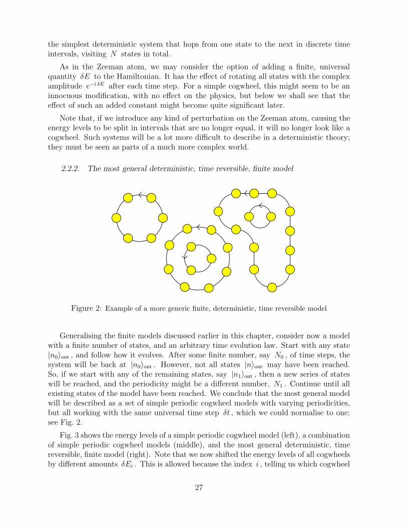
2 Example of a more generic finite, deterministic, time reversible model . . . . . . 27

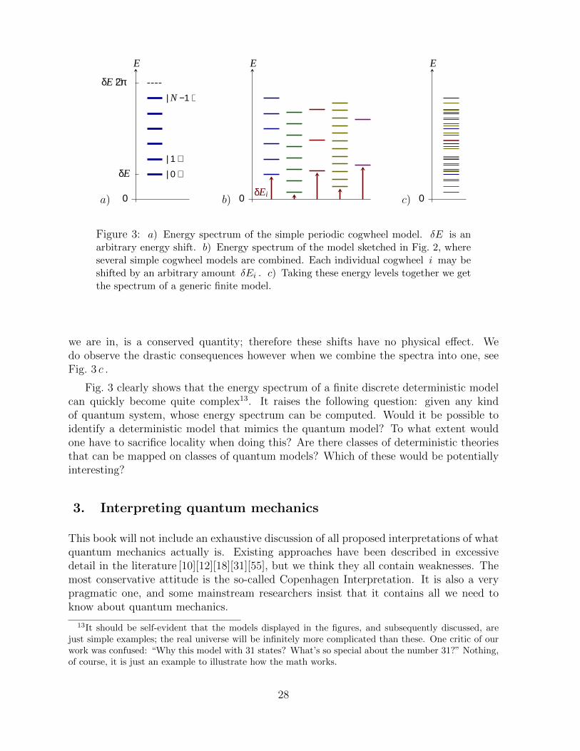
3 a) Energy spectrum of the simple periodic cogwheel model. b) Energy spectrum

of various cogwheels. c) Energy spectrum of composite model of Fig. 2. . . . . 28

4 A bell-type experiment. Space runs horizontally, time vertically. . . . . . . . . 39

5 The mouse dropping function, Eq. (3.26). . . . . . . . . . . . . . . . . . . . . 43

6 a) The ontological sub-microscopic states, the templates and the classical states.

b) Classical states are (probabilistic) distributions of the sub-microscopic states. 50

7

7 a) Simple 5-state automaton model with information loss. b) Its three equiva-

lence classes. c) Its three energy levels. . . . . . . . . . . . . . . . . . . . . . 82

8 Example of a more generic finite, deterministic, time non reversible model. . . 83

9 a) Plot of the inner products 〈m3|m1〉 ; b) Plot of the transformation matrix

〈m1|σ〉ont (real part). Horiz.: m1 , vert.: σ . . . . . . . . . . . . . . . . . . . 121

10 The spectrum of the Hamiltonian in various expansions. . . . . . . . . . . . . . 123

11 The “second quantised” version of the multiple-cogwheel model of Fig. 2. . . . 127

12 The beables for the “neutrino”. . . . . . . . . . . . . . . . . . . . . . . . . . 134

13 The wave function of the state (P,Q) = (0, 0) , and the asymptotic form of some

small peaks. . . . . . . . . . . . . . . . . . . . . . . . . . . . . . . . . . . . 152

14 The spectrum of allowed values of the quantum string coordinates. . . . . . . . 180

15 Deterministic string interaction. . . . . . . . . . . . . . . . . . . . . . . . . . 188

16 Rotations in the Brillouin zone of a rectangular lattice. . . . . . . . . . . . . . 193

17 The function Kd (y) , a) for d = 2 , and b) for d = 5 . . . . . . . . . . . . . . 194

18 The Brillouin zones for the lattice momentum ~κ of the ontological model de-

scribed by Eq. (18.29) in two dimensions. a) the ontological model, b) its

Hilbert space description. . . . . . . . . . . . . . . . . . . . . . . . . . . . . 199

19 The QP lattice in the 1+1 dimensional case. . . . . . . . . . . . . . . . . . . 209

20 A small region in the QP lattice where the (integer valued) Hamiltonian is

reasonably smooth . . . . . . . . . . . . . . . . . . . . . . . . . . . . . . . . 210

21 The angle cut out of space when a particle moves with velocity ξ . . . . . . . . 247

Preface

This book is not in any way intended to serve as a replacement for the standard theoryof quantum mechanics. A reader not yet thoroughly familiar with the basic concepts ofquantum mechanics is advised first to learn this theory from one of the recommended textbooks [15][16][37], and only then pick up this book to find out that the doctrine called‘quantum mechanics’ can be viewed as part of a marvellous mathematical machinery thatplaces physical phenomena in a greater context, and only in the second place as a theoryof nature.

The present version, # 3, has been thoroughly modified. Some novelties, such as anunconventional view of the arrow of time, have been added, and other arguments werefurther refined. The book is now split in two. Part I deals with the many conceptualissues, without demanding excessive calculations. Part II adds to this our calculationtechniques, occasionally returning to conceptual issues. Inevitably, the text in both parts

8

will frequently refer to discussions in the other part, but they can be studied separately.

This book is not a novel that has to be read from beginning to end, but rather acollection of descriptions and derivations, to be used as a reference. Different parts canbe read in random order. Some arguments are repeated several times, but each time in adifferent context.

Part I

The Cellular Automaton Interpretation as a general

doctrine

1. Motivation for this work

This book is about a theory, and about an interpretation. The theory, as it stands, ishighly speculative. It is born out of dissatisfaction with the existing explanations of awell-established fact. The fact is that our universe appears to be controlled by the lawsof quantum mechanics. Quantum mechanics looks weird, but nevertheless it provides fora very solid basis for doing calculations of all sorts that explain the peculiarities of theatomic and sub-atomic world. The theory developed in this book starts from assumptionsthat, at first sight, seem to be natural and straightforward, and we think they can be verywell defended.

Regardless whether the theory is completely right, partly right, or dead wrong, one maybe inspired by the way it looks at quantum mechanics. We are assuming the existence of adefinite ‘reality’ underlying quantum mechanical descriptions. The assumption that thisreality exists leads to a rather down-to-earth interpretation of what quantum mechanicalcalculations are telling us. The interpretation works beautifully and seems to removeseveral of the difficulties encountered in other descriptions of how one might interpretthe measurements and their findings. We propose this interpretation that, in our eyes, issuperior to other existing dogmas.

However, numerous extensive investigations have provided very strong evidence thatthe assumptions that went into our theory cannot be completely right. The earliest argu-ments came from von Neumann [5], but these were later hotly debated [7],[18],[60]. Themost convincing arguments came from John S. Bell’s theorem, phrased in terms of in-equalities that are supposed to hold for any classical interpretation of quantum mechanics,but are strongly violated by quantum mechanics. Later, many other variations were foundof Bell’s basic idea, some even more powerful. We will discuss these repeatedly, and atlength, in this work. Basically, they all seemed to point in the same direction: from thesetheorems, it was concluded by most researchers that the laws of nature cannot possibly

9

be deterministic. So why this book?

There are various reasons why the author decided to hold on to his assumptionsanyway. The first reason is that they fit very well with the quantum equations of variousvery simple models. It looks as if nature is telling us: “wait, this approach is not so badat all!”. The second reason is that one could regard our approach simply as a first attemptat a description of nature that is more realistic than other existing approaches. We canalways later decide to add some twists that introduce indeterminism, in a way more inline with the afore mentioned theorems; these twists could be very different from what isexpected by many experts, but anyway, in that case, we could all emerge out of this fightvictorious. Perhaps there is a subtle form of non-locality in the cellular automata, perhapsthere is some quantum twist in the boundary conditions, or you name it. Why shouldBell’s inequalities forbid me to investigate this alley? I happen to find it an interestingone.

But there is a third reason. This is the strong suspicion that all those “hidden variablemodels” that were compared with thought experiments as well as real experiments, areterribly naive.1 Real deterministic theories have not yet been excluded. If a theory isdeterministic all the way, it implies that not only all observed phenomena, but also theobservers themselves are controlled by deterministic laws. They certainly have no ‘freewill’, their actions all have roots in the past, even the distant past. Allowing an observerto have free will, that is, to reset his observation apparatus at will without even infinites-imal disturbances of the surrounding universe, including modifications in the distant past,is fundamentally impossible. The notion that, also the actions by experimenters and ob-servers are controlled by deterministic laws, is called superdeterminism. When discussingthese issues with colleagues the author got the distinct impression that it is here that the‘no-go’ theorems they usually come up with, can be put in doubt.

We hasten to add that this is not the first time that this remark was made [61]. Bellnoticed that superdeterminism could provide for a loophole around his theorem, but asmost researchers also today, he was quick to dismiss it as “absurd”. As we hope to beable to demonstrate, however, superdeterminism may not quite be as absurd as it seems.2

In any case, realising these facts sheds an interesting new light on our questions, andthe author was strongly motivated just to carry on.

Having said all this, I do admit that what we have is still only a theory. It can andwill be criticised and attacked, as it already was. I know that some readers will not beconvinced. If, in the mind of some others, I succeed to generate some sympathy, evenenthusiasm for these ideas, then my goal has been reached. In a somewhat worse scenario,my ideas will be just used as an anvil, against which other investigators will sharpen theirown, superior views.

In the mean time, we are developing mathematical notions that seem to be coherentand beautiful. Not very surprisingly, we do encounter some problems in the formalism

1Indeed, in their eagerness to exclude local, realistic, and/or deterministic theories, authors rarely gointo the trouble to carefully define what these theories are.

2We do find some “absurd” correlation functions, see e.g. subsection 3.6.2.

10

as well, which we try to phrase as accurately as possible. They do indicate that theproblem of generating quantum phenomena out of classical equations is actually quitecomplex. The difficulty we bounce into is that, although all classical models allow fora reformulation in terms of some ‘quantum’ system, the resulting quantum system willoften not have a Hamiltonian that is local and properly bounded from below. It maywell be that models that do produce acceptable Hamiltonians will demand inclusion ofnon-perturbative gravitational effects, which are indeed difficult and ill-understood atpresent.

It is unlikely, in the mind of the author, that these complicated schemes can be wipedoff the table in a few lines, as is asserted by some3. Instead, they warrant intensiveinvestigation. As stated, if we can make the theories more solid, they would provide forextremely elegant foundations that underpin the Cellular Automaton Interpretation ofquantum mechanics. It will be shown in this book that we can arrive at Hamiltoniansthat are almost both local and bounded from below. These models are like quantised fieldtheories, which also suffer from mathematical imperfections, as is well-known.

Furthermore, one may question why we would have to require locality of the quantummodel at all, as long as the underlying classical model is manifestly local by construction.What we exactly mean by all this will be explained, mostly in part II where we allowourselves to perform detailed calculations.

1.1. Why an interpretation is needed

The discovery of quantum mechanics may well have been the most important scientificrevolution of the 20th century. Not only the world of atoms and subatomic particlesappears to be completely controlled by the rules of quantum mechanics, but also the worldsof solid state physics, chemistry, thermodynamics, and all radiation phenomena can onlybe understood by observing the laws of the quanta. The successes of quantum mechanicsare phenomenal, and furthermore, the theory appears to be reigned by marvellous andimpeccable internal mathematical logic.

Not very surprisingly, this great scientific achievement also caught the attention ofscientists from other fields, and from philosophers, as well as the public in general. It istherefore perhaps somewhat curious that, even after nearly a full century, physicists stilldo not quite agree on what the theory tells us – and what it does not tell us – aboutreality.

The reason why quantum mechanics works so well is that, in practically all areasof its applications, exactly what reality means turns out to be immaterial. All thatthis theory4 says, and that needs to be said, is about the reality of the outcomes of anexperiment. Quantum mechanics tells us exactly what one should expect, how these

3At various places in this book, we explain what is wrong with those ‘few lines’.4Interchangeably, we use the word ‘theory’ for quantum mechanics itself, and for models of particle

interactions; therefore, it might be better to refer to quantum mechanics as a framework, assisting usin devising theories for sub systems, but we expect that our use of the concept of ‘theory’ should notgenerate any confusion.

11

outcomes may be distributed statistically, and how these can be used to deduce detailsof its internal parameters. Elementary particles are one of the prime targets here. Atheory4 has been arrived at, the so-called Standard Model, that requires the specificationof some 25 internal constants of nature, parameters that cannot be predicted using presentknowledge. Most of these parameters could be determined from the experimental results,with varied accuracies. Quantum mechanics works flawlessly every time.

So, quantum mechanics, with all its peculiarities, is rightfully regarded as one of themost profound discoveries in the field of physics, revolutionising our understanding ofmany features of the atomic and sub-atomic world.

But physics is not finished. In spite of some over-enthusiastic proclamations justbefore the turn of the century, the Theory of Everything has not yet been discovered,and there are other open questions reminding us that physicists have not yet done theirjob completely. Therefore, encouraged by the great achievements we witnessed in thepast, scientists continue along the path that has been so successful. New experimentsare being designed, and new theories are developed, each with ever increasing ingenuityand imagination. Of course, what we have learned to do is to incorporate every piece ofknowledge gained in the past, in our new theories, and even in our wilder ideas.

But then, there is a question of strategy. Which roads should we follow if we wish toput the last pieces of our jig-saw puzzle in place? Or even more to the point: what dowe expect those last jig-saw pieces to look like? And in particular: should we expect theultimate future theory to be quantum mechanical?

It is at this point that opinions among researchers vary, which is how it should be inscience, so we do not complain about this. On the contrary, we are inspired to searchwith utter concentration precisely at those spots where no-one else has taken the troubleto look before. The subject of this book is the ‘reality’ behind quantum mechanics. Oursuspicion is that it may be very different from what can be read in most text books. Weactually advocate the notion that it might be simpler than anything that can be readin the text books. If this is really so, this might greatly facilitate our quest for bettertheoretical understanding.

Many of the ideas expressed and worked out in this treatise are very basic. Clearly,we are not the first to advocate these ideas. The reason why one rarely hears about theobvious and simple observations that we will make, is that they have been made manytimes, in the recent and the more ancient past [5], and were subsequently categoricallydismissed.

The primary reason why they have been dismissed is that they were unsuccessful;classical, deterministic models that produce the same results as quantum mechanics weredevised, adapted and modified, but whatever was attempted ended up looking much uglierthan the original theory, which was plain quantum mechanics with no further questionsasked. The quantum mechanical theory describing relativistic, subatomic particles iscalled quantum field theory (see part II, chapter 20), and it obeys fundamental conditionssuch as causality, locality and unitarity. Demanding all of these desirable properties wasthe core of the successes of quantum field theory, and that eventually gave us the Standard

12

Model of the sub-atomic particles. If we try to reproduce the results of quantum fieldtheory in terms of some deterministic underlying theory, it seems that one has to abandonat least one of these demands, which would remove much of the beauty of the generallyaccepted theory; it is much simpler not to do so, and therefore, as for the requirement ofthe existence of a classical underlying theory, one usually simply drops that.

Not only does it seem to be unnecessary to assume the existence of a classical worldunderlying quantum mechanics, it seems to be impossible also. Not very surprisingly,researchers turn their heads in disdain, but just before doing so, there was one morething to do: if, invariably, deterministic models that were intended to reproduce typicallyquantum mechanical effects, appear to get stranded in contradictions, maybe one canprove that such models are impossible. This may look like the more noble alley: close thedoor for good.

A way to do this was to address the famous Gedanken experiment designed by Einstein,Podolsky and Rosen [6]. This experiment suggested that quantum particles are associatedwith more than just a wave function; to make quantum mechanics describe ‘reality’, somesort of ‘hidden variables’ seemed to be needed. What could be done was to prove thatsuch hidden variables are self-contradictory. We call this a ‘no-go theorem’. The mostnotorious, and most basic, example was Bell’s theorem [18], as we already mentioned. Bellstudied the correlations between measurements of entangled particles, and found that, ifthe initial state for these particles is chosen to be sufficiently generic, the correlationsfound at the end of the experiment, as predicted by quantum mechanics, can never bereproduced by information carriers that transport classical information. He expressedthis in terms of the so-called Bell inequalities, later extended as CHSH inequality [20].They are obeyed by any classical system but strongly violated by quantum mechanics. Itappeared to be inevitable to conclude that we have to give up producing classical, local,realistic theories. They don’t exist.

So why the present treatise? Almost every day, we receive mail from amateur physi-cists telling us why established science is all wrong, and what they think a “theory ofeverything” should look like. Now it may seem that I am treading in their foot steps. AmI suggesting that nearly one hundred years of investigations of quantum mechanics havebeen wasted? Not at all. I insist that the last century of research lead to magnificentresults, and that the only thing missing so-far was a more radical description of what hasbeen found. Not the equations were wrong, not the technology, but only the wording ofwhat is often referred to as the Copenhagen Interpretation should be replaced. Up totoday, the theory of quantum mechanics consisted of a set of very rigorous rules as to howamplitudes of wave functions refer to the probabilities for various different outcomes ofan experiment. It was stated emphatically that they are not referring to ‘what is reallyhappening’. One should not ask what is really happening, one should be content with thepredictions concerning the experimental results. The idea that no such ‘reality’ shouldexist at all sounds mysterious. It is my intention to remove every single bit of mysticismfrom quantum theory, and we intend to deduce facts about reality anyway.

Quantum mechanics is one of the most brilliant results of one century of science,and it is not my intention to replace it by some mutilated version, no matter how slight

13

the mutilation would be. Most of the text books on quantum mechanics will not needthe slightest revision anywhere, except perhaps when they state that questions aboutreality are forbidden. All practical calculations on the numerous stupefying quantumphenomena can be kept as they are. It is indeed in quite a few competing theories aboutthe interpretation of quantum mechanics where authors are led to introduce non-linearitiesin the Schrodinger equation or violations of the Born rule that will be impermissible inthis work.

As for ‘entangled particles’, since it is known how to produce such states in practice,their odd-looking behaviour must be completely taken care of in our approach.

The ‘collapse of the wave function’ is a typical topic of discussion, where several re-searchers believe a modification of Schrodinger’s equation is required. Not so in this work,as we shall explain. We also find surprisingly natural answers to questions concerning‘Schrodinger’s cat’, and the ‘arrow of time’.

And as of ‘no-go theorems’, this author has seen several of them, standing in the wayof further progress. One always has to take the assumptions into consideration, just asthe small print in a contract.

1.2. Outline of the ideas exposed in part I

Our starting point will be extremely simple and straightforward, in fact so much so thatsome readers may simply conclude that I am losing my mind. However, with questionsof the sort I will be asking, it is inevitable to start at the very basic beginning. We startwith just any classical system that vaguely looks like our universe, with the intention torefine it whenever we find this to be appropriate. Will we need non-local interactions?Will we need information loss? Must we include some version of a gravitational force? Orwill the whole project run astray? We won’t know unless we try.

The price we do pay seems to be a modest one, but it needs to be mentioned: we haveto select a very special set of mutually orthogonal states in Hilbert space that are endowedwith the status of being ‘real’. This set consists of the states the universe can ‘really’be in. At all times, the universe chooses one of these states to be in, with probability1, while all others carry probability 0. We call these states ontological states, and theyform a special basis for Hilbert space, the ontological basis. One could say that this isjust wording, so this price we pay is affordable, but we will assume this very special basisto have special properties. What this does imply is that the quantum theories we end upwith all form a very special subset of all quantum theories. This then, could lead to newphysics, which is why we believe our approach will warrant attention: eventually, our aimis not just a reinterpretation of quantum mechanics, but the discovery of new tools formodel building.

One might expect that our approach, having such a precarious relationship with bothstandard quantum mechanics and other insights concerning the interpretation of quantummechanics, should quickly strand in contradictions. This is perhaps the more remarkableobservation one then makes: it works quite well! Several models can be constructed that

14

reproduce quantum mechanics without the slightest modification, as will be shown in muchmore detail in part II. All our simple models are quite straightforward. The numerousresponses I received, saying that the models I produce “somehow aren’t real quantummechanics” are simply mistaken. They are really quantum mechanical. However, I willbe the first to remark that one can nonetheless criticise our results: the models are eithertoo simple, which means they do not describe interesting, interacting particles, or theyseem to exhibit more subtle defects. In particular, reproducing realistic quantum modelsfor locally interacting quantum particles along the lines proposed, has as yet shown tobe beyond what we can do. As an excuse I can only plead that this would require notonly the reproduction of a complete, renormalizable quantum field theoretical model, butin addition it may well demand the incorporation of a perfectly quantised version of thegravitational force, so indeed it should not surprise anyone that this is hard.

Numerous earlier attempts have been made to find holes in the arguments initiatedby Bell, and corroborated by others. Most of these falsification arguments have beenrightfully dismissed. But now it is our turn. Knowing what the locality structure isexpected to be in our models, and why we nevertheless think they reproduce quantummechanics, we can now attempt to locate the cause of this apparent disagreement. Is thefault in our models or in the arguments of Bell c.s.? What could be the cause of thisdiscrepancy? If we take one of our classical models, what goes wrong in a Bell experimentwith entangled particles? Were assumptions made that do not hold? Do particles in ourmodels perhaps refuse to get entangled? This way, we hope to contribute to an ongoingdiscussion.

The aim of the present study is to work out some fundamental physical principles.Some of them are nearly as general as the fundamental, canonical theory of classicalmechanics. The way we deviate from standard methods is that, more frequently thanusual, we introduce discrete kinetic variables. We demonstrate that such models notonly appear to have much in common with quantum mechanics. In many cases, they arequantum mechanical, but also classical at the same time. Some of our models occupya domain in between classical and quantum mechanics, a domain often thought to beempty.

Will this lead to a revolutionary alternative view on what quantum mechanics is? Thedifficulties with the sign of the energy and the locality of the effective Hamiltonians inour theories have not yet been settled. In the real world there is a lower bound for thetotal energy, so that there is a vacuum state. The subtleties associated with that arepostponed to part II, since they require detailed calculations. In summary: we suspectthat there will be several ways to overcome this difficulty, or better still, that it can beused to explain some of the apparent contradictions in quantum mechanics.

The complete and unquestionable answers to many questions are not given in thistreatise, but we are homing in to some important observations. As has happened inother examples of “no-go theorems”, Bell and his followers did make assumptions, and intheir case also, the assumptions appeared to be utterly reasonable. Nevertheless we nowsuspect that some of the premises made by Bell may have to be relaxed. Our theory is notyet complete, and a reader strongly opposed to what we are trying to do here, may well

15

be able to find a stick that seems suitable to destroy it. Others, I hope, will be inspiredto continue along this path.

We invite the reader to draw his or her own conclusions. We do intend to achievethat questions concerning the deeper meanings of quantum mechanics are illuminatedfrom a new perspective. This we do by setting up models and by doing calculations inthese models. Now this has been done before, but most models I have seen appear tobe too contrived, either requiring the existence of infinitely many universes all interferingwith one another, or modifying the equations of quantum mechanics, while the originalequations seem to be beautifully coherent and functional.

Our models suggest that Einstein may have been right, when he objected againstthe conclusions drawn by Bohr and Heisenberg. It may well be that, at its most basiclevel, there is no randomness in nature, no fundamentally statistical aspect to the lawsof evolution. Everything, up to the most minute detail, is controlled by invariable laws.Every significant event in our universe takes place for a reason, it was caused by the actionof physical law, not just by chance. This is the general picture conveyed by this book.We know that it looks as if Bell’s inequalities have refuted this possibility, so yes, theyraise interesting and important questions that we shall address at various levels.

It may seem that I am employing rather long arguments to make my point5. The mostessential elements of our reasoning will show to be short and simple, but just because Iwant chapters of this book to be self-sustained, well readable and understandable, therewill be some repetitions of arguments here and there, for which I apologise. I also apologisefor the fact that some parts of the calculations are at a very basic level; the hope is thatthis will also make this work accessible for a larger class of scientists and students.

The most elegant way to handle quantum mechanics in all its generality is Dirac’sbra-ket formalism (section 1.4). We stress that Hilbert space is a central tool for physics,not only for quantum mechanics. It can be applied in much more general systems thanthe standard quantum models such as the hydrogen atom, and it will be used also in com-pletely deterministic models (we can even use it in Newton’s description of the planetarysystem, see subsection 5.7.1).

In any description of a model, one first chooses a basis in Hilbert space. Then, what isneeded is a Hamiltonian, in order to describe dynamics. A very special feature of Hilbertspace is that one can use any basis one likes. The transformation from one basis to anotheris a unitary transformation, and we shall frequently make use of such transformations.Everything written about this in sections 1.4, 3.1 and 11.3 is completely standard.

In part I of the book, we describe the philosophy of the Cellular Automaton Interpre-tation (CAI) without too many technical calculations. After the Introduction, we firstdemonstrate the most basic prototype of a model, the Cogwheel Model, in chapter 2.

In chapters 3 and 4, we begin to deal with the real subject of this research: the questionof the interpretation of quantum mechanics. The standard approach, referred to as theCopenhagen Interpretation, is dealt with very briefly, emphasising those points where we

5A wise lesson to be drawn from one’s life experiences is, that long arguments are often much moredubious than short ones.

16

have something to say, in particular the Bell and the CHSH inequalities.

Subsequently, we formulate as clearly as possible what we mean with determinis-tic quantum mechanics. The Cellular Automaton Interpretation of quantum mechanics(chapters 4 and 5) must sound as a blasphemy to some quantum physicists, but this isbecause we do not go along with some of the assumptions usually made. Most notably, itis the assumption that space-like correlations in the beables of this world cannot possiblygenerate the ‘conspiracy’ that seems to be required to violate Bell’s inequality. We derivethe existence of such correlations.

We end chapter 3 with one of the more important fundamental ideas of the CAI: ourhidden variables do contain ‘hidden information’ about the future, notably the settingsthat will be chosen by Alice an Bob, but it is fundamentally non-local information, impos-sible to harvest even in principle (subsection 3.6.2). This should not be seen as a violationof causality.

Even if it is still unclear whether or not the results of these correlations have a con-spiratory nature, one can base a useful and functional interpretation doctrine from theassumption that the only conspiracy the equations perform is to fool some of today’sphysicists, while they act in complete harmony with credible sets of physical laws. Themeasurement process and the collapse of the wave function are two riddles that are com-pletely resolved by this assumption, as will be indicated.

We hope to inspire more physicists to investigate these possibilities, to consider seri-ously the possibility that quantum mechanics as we know it is not a fundamental, mysteri-ous, impenetrable feature of our physical world, but rather an instrument to statisticallydescribe a world where the physical laws, at their most basic roots, are not quantummechanical at all. Sure, we do not know how to formulate the most basic laws at present,but we are collecting indications that a classical world underlying quantum mechanicsdoes exist.

Our models show how to put quantum mechanics on hold when we are constructingmodels such as string theory and “quantum” gravity, and this may lead to much improvedunderstanding of our world at the Planck scale. Many chapters are reasonably self sus-tained; one may choose to go directly to the parts where the basic features of the CellularAutomaton Interpretation (CAI) are exposed, chapters 3 – 10, or look at the explicitcalculations done in part II.

In chapter 5.2, we display the rules of the game. Readers might want to jump to thischapter directly, but might then be mystified by some of our assertions if one has notyet been exposed to the general working philosophy developed in the previous chapters.Well, you don’t have to take everything for granted; there are still problems unsolved,and further alleys to be investigated. They are in chapter 9, where it can be seen howthe various issues show up in calculations.

Part II of this book is not intended to impress the reader or to scare him or heraway. The explicit calculations carried out there are displayed in order to develop anddemonstrate our calculation tools; only few of these results are used in the more generaldiscussions in the first part. Just skip them if you don’t like them.

17

1.3. A 19 th century philosophy

Let us go back to the 19th century. Imagine that mathematics were at a very advancedlevel, but nothing of the 20th century physics was known. Suppose someone had phrased adetailed hypothesis about his world being a cellular automaton6. The cellular automatonwill be precisely defined in section 5.1 and in part II; for now, it suffices to characteriseit by the requirement that the states Nature can be in are given by sequences of integers.The evolution law is a classical algorithm that tells unambiguously how these integersevolve in time. Quantum mechanics does not enter; it is unheard of. The evolution law issufficiently non-trivial to make our cellular automaton behave as a universal computer [35].This means that, at its tiniest time and distance scale, initial states could be chosensuch that any mathematical equation can be solved with it. This means that it will beimpossible to derive exactly how the automaton will behave at large time intervals; it willbe far too complex.

Mathematicians will realise that one should not even try to deduce exactly what thelarge-time and large-distance properties of this theory will be, but they may decide to trysomething else. Can one, perhaps, make some statistical statements about the large scalebehaviour?

In first approximation, just white noise may be seen to emerge, but upon closer in-spection, the system may develop non-trivial correlations in its series of integers; some ofthe correlation functions may be calculable, just the way these may be calculated in a Vander Waals gas. We cannot rigorously compute the trajectories of individual molecules inthis gas, but we can derive free energy and pressure of the gas as a function of densityand temperature, we can derive its viscosity and other bulk properties. Clearly, this iswhat our 19th century mathematicians should do with their cellular automaton modelof their world. In this book we will indicate how physicists and mathematicians of the20th and 21st centuries can do even more: they have a tool called quantum mechanics toderive and understand even more sophisticated details, but even they will have to admitthat exact calculations are impossible. The only effective, large scale laws that they canever expect to derive are statistical ones. The average outcomes of experiments can bepredicted, but not the outcomes of individual experiments; for doing that, the evolutionequations are far too difficult to handle.

In short, our imaginary 19th century world will seem to be controlled by effectivelaws with a large stochastic element in them. This means that, in addition to an effectivedeterministic law, random number generators may seem to be at work that are funda-mentally unpredictable. On the face of it, these effective laws together may look quite abit like the quantum mechanical laws we have today for the sub-atomic particles.

The above metaphor is of course not perfect. The Van der Waals gas does obey generalequations of state, one can understand how sound waves behave in such a gas, but it isnot quantum mechanical. One could suspect that this is because the microscopic lawsassumed to be at the basis of a Van der Waals gas are very different from a cellular

6One such person is E. Fredkin, an expert in numerical computation techniques, with whom we hadlengthy discussions. The idea itself was of course much older [19][52].

18

automaton, but it is not known whether this might be sufficient to explain why the Vander Waals gas is clearly not quantum mechanical.

What we do wish to deduce from this reasoning is that one feature of our world isnot mysterious: the fact that we have effective laws that require a stochastic elementin the form of an apparently perfect random number generator, is something we shouldnot be surprised about. Our 19th century physicists would be happy with what theirmathematicians give them, and they would have been totally prepared for the findings of20th century physicists, which implied that indeed the effective laws controlling hydrogenatoms contain a stochastic element, for instance to determine at what moment exactly anexcited atom decides to emit a photon.

This may be the deeper philosophical reason why we have quantum mechanics: notall features of the cellular automaton at the basis of our world allow to be extrapolated tolarge scales. Clearly, the exposition of this chapter is entirely non-technical and it may bea bad representation of all the subtleties of the theory we call quantum mechanics today.Yet we think it already captures some of the elements of the story we want to tell. Ifthey had access to the mathematics known today, we may be led to the conclusion thatour 19th century physicists could have been able to derive an effective quantum theoryfor their automaton model of the world. Would the 19th century physicists be able todo experiments with entangled photons? This question we postpone to section 3.6 andonwards.

Philosophising about the different turns the course of history could have chosen, imag-ine the following. In the 19th century, the theory of atoms already existed. They couldhave been regarded as physicists’ first successful step to discretise the world: atoms arethe quanta of matter. Yet energy, momenta, and angular momenta were still assumed tobe continuous. Would it not have been natural to suspect these to be discrete as well? Inour world, this insight came with the discovery of quantum mechanics. But even today,space and time themselves are still strictly continuous entities. When will we discover thateverything in the physical world will eventually be discrete? This would be the discrete,deterministic world underlying our present theories. In this scenario, quantum mechanicsas we know it, is the imperfect logic resulting from an incomplete discretisation7.

1.4. Notation

In most parts of this book, quantum mechanics will be used as a tool kit, not a theory.Our theory may be anything; one of our tools will be Hilbert space and the mathematicalmanipulations that can be done in that space. Although we do assume the reader to befamiliar with these concepts, we briefly recapitulate what a Hilbert space is.

Hilbert space H is a complex8 vector space, whose number of dimensions is usually

7As I write this, I expect numerous letters by amateurs, but beware, as it would be easy to proposesome completely discretized concoction, but it is very hard to find the right theory, one that helps us tounderstand the world as it is using rigorous mathematics.

8Some critical readers were wondering where the complex numbers in quantum mechanics should comefrom, given the fact that we start off from classical theories. The answer is simple: complex numbers

19

infinite, but sometimes we allow that to be a finite number. Its elements are called states,denoted as |ψ〉, |ϕ〉 , or any other “ket”.

We have linearity : whenever |ψ1〉 and ψ2〉 are states in our Hilbert space, then

|ϕ〉 = λ|ψ1〉+ µ|ψ2〉 , (1.1)

where λ and µ are complex numbers, is also a state in this Hilbert space. For everyket-state |ψ〉 we have a ‘conjugated bra-state’, 〈ψ| , spanning a conjugated vector space,〈ψ|, 〈ϕ| . This means that, if Eq. (1.1) holds, then

〈ϕ| = λ∗〈ψ1|+ µ∗〈ψ2| . (1.2)

Furthermore, we have an inner product, or inproduct: if we have a bra, 〈χ| , and a ket,|ψ〉 , then a complex number is defined, the inner product denoted by 〈χ|ψ〉 , obeying

〈χ|(λ|ψ1〉+ µ|ψ2〉) = λ〈χ|ψ1〉+ µ〈χ|ψ2〉 ; 〈χ|ψ〉 = 〈ψ|χ〉∗ . (1.3)

The inner product of a ket state |ψ〉 with its own bra is real and positive:

‖ψ‖2 ≡ 〈ψ|ψ〉 = real and ≥ 0 , (1.4)

while 〈ψ|ψ〉 = 0 ↔ |ψ〉 = 0 . (1.5)

Therefore, the inner product can be used to define a norm. A state |ψ〉 is called a physicalstate, or normalised state, if

‖ψ‖2 = 〈ψ|ψ〉 = 1 . (1.6)

Later, we shall use the word template to denote such state (the word ‘physical state’ wouldbe confusing and is better to be avoided). The full power of Dirac’s notation is exploitedfurther in part II.

Variables will sometimes be just numbers, and sometimes operators in Hilbert space.If the distinction should be made, or if clarity may demand it, operators will be denotedas such. We decided to do this simply by adding a super- or subscript “op” to the symbolin question.9

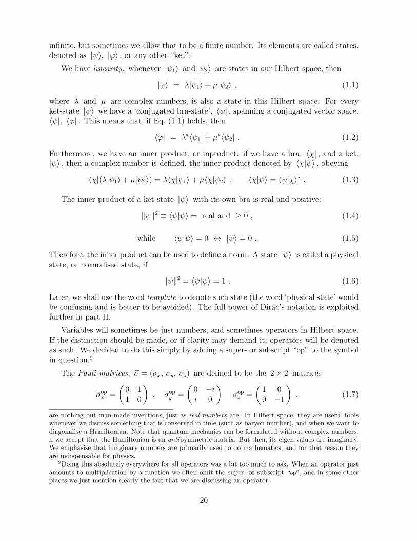
The Pauli matrices, ~σ = (σx, σy, σz) are defined to be the 2× 2 matrices

σopx =

(0 11 0

), σop

y =

(0 −ii 0

)σopz =

(1 00 −1

). (1.7)

are nothing but man-made inventions, just as real numbers are. In Hilbert space, they are useful toolswhenever we discuss something that is conserved in time (such as baryon number), and when we want todiagonalise a Hamiltonian. Note that quantum mechanics can be formulated without complex numbers,if we accept that the Hamiltonian is an anti symmetric matrix. But then, its eigen values are imaginary.We emphasise that imaginary numbers are primarily used to do mathematics, and for that reason theyare indispensable for physics.

9Doing this absolutely everywhere for all operators was a bit too much to ask. When an operator justamounts to multiplication by a function we often omit the super- or subscript “op”, and in some otherplaces we just mention clearly the fact that we are discussing an operator.

20

2. Deterministic models in quantum notation

2.1. The basic structure of deterministic models

For deterministic models, we will be using the same Dirac notation. A physical state |A〉 ,where A may stand for any array of numbers, not necessarily integers or real numbers,is called an ontological state if it is a state our deterministic system can be in. Thesestates themselves do not form a Hilbert space, since in a deterministic theory we have nosuperpositions, but we can declare that they form a basis for a Hilbert space that we mayherewith define [70][73], by deciding, once and for all, that all ontological states form anorthonormal set:

〈A|B〉 ≡ δAB . (2.1)

We can allow this set to generate a Hilbert space if we declare what we mean when wetalk about superpositions. In Hilbert space, we now introduce the quantum states |ψ〉 ,as being more general than the ontological states:

|ψ〉 =∑A

λA|A〉 ,∑A

|λA|2 ≡ 1 . (2.2)

A quantum state can be used as a template for doing physics. With this we mean thefollowing:

A template is a quantum state of the form (2.2) describing a situation wherethe probability to find our system to be in the ontological state |A〉 is |λA|2 .

Note, that λA is allowed to be a complex or negative number, whereas the phase of λAplays no role whatsoever. In spite of this, complex numbers will turn out to be quiteuseful here, as we shall see. Using the square in Eq. (2.2) and in our definition above, isa fairly arbitrary choice; in principle, we could have used a different power. Here, we usethe squares because this is by far the most useful choice; different powers would not affectthe physics, but would result in unnecessary mathematical complications. The squaresensure that probability conservation amounts to a proper normalisation of the templatestates, and enable the use of unitary matrices in our transformations.

Occasionally, we may allow the indicators A, B, · · · to represent continuous variables,a straightforward generalisation. In that case, we have a continuous deterministic system;the Kronecker delta in Eq. (2.1) is then replaced by a Dirac delta, and the sums in Eq. (2.2)will be replaced by integrals. For now, to be explicit, we stick to a discrete notation.

We emphasise that the template states are not ontological. Hence we have no directinterpretation, as yet, for the inner products 〈ψ1|ψ2〉 if both |ψ1〉 and |ψ2〉 are templatestates. Only the absolute squares of 〈A|ψ〉 , where 〈A| is the conjugate of an ontologicalstate, denote the probabilities |λA|2 . We briefly return to this in subsection 5.5.3.

The time evolution of a deterministic model can now be written in operator form:

|A(t)〉 = |P (t)op A(0)〉 , (2.3)

21

where P(t)op is a permutation operator. We can write P

(t)op as a matrix P

(t)AB containing

only ones and zeros. Then, Eq. (2.3) is written as a matrix equation,

|A(t〉) = UAB(t)|B(0)〉 , U(t)AB = P(t)AB . (2.4)

By definition therefore, the matrix elements of the operator U(t) in this bases can onlybe 0 or 1.

It is very important, at this stage, that we choose P(t)op to be a genuine permutator,

that is, it should be invertible.10 If the evolution law is time-independent, we have

P (t)op =

(P (δt)

op

)t/δt, Uop(t) =

(Uop(δt)

)t/δt, (2.5)

where the permutator P(δt)op , and its associated matrix Uop(δt) describe the evolution

over the shortest possible time step, δt .

Note, that no harm is done if some of the entries in the matrix U(δt)ab , instead of 1,are chosen to be unimodular complex numbers. Usually, however, we see no reason to doso, since a simple rotation of an ontological state in the complex plane has no physicalmeaning, but it could be useful for doing mathematics (for example, in section 15 of partII, we use the entries ±1 and 0 in our evolution operators).

We can now state our first important mathematical observation:The quantum-, or template-, states |ψ〉 all obey the same evolution equation:

|ψ(t)〉 = Uop(t)|ψ(0)〉 . (2.6)

It is easy to observe that, indeed, the probabilities |λA|2 evolve as expected.11

Much of the work described in this book will be about writing the evolution operatorsUop(t) as exponentials: Find a hermitean operator Hop such that

Uop(δt) = e−iHop δt , so that Uop(t) = e−iHopt . (2.7)

This elevates the time variable t to be continuous, if it originally could only be a multipleof δt . Finding an example of such an operator is actually easy. If, for simplicity, werestrict ourselves to template states |ψ〉 that are orthogonal to the eigenstate of Uop

with eigenvalue 1, then

Hop δt = π − i∞∑n=1

1

n(Uop(n δt)− Uop(−n δt)) (2.8)

is a solution of Eq. (2.7). This equation can be checked by Fourier analysis, see part II,section 12.2, Eqs (12.8) – (12.10).

10One can imagine deterministic models where P(t)op does not have an inverse, which means that two

different ontological states might both evolve into the same state later. We will consider this possibilitylater, see chapter 7.

11At this stage of the theory, one may still define probabilities to be given as different functions of λA ,in line with the observation just made after Eq. (2.2).

22

Note that a correction is needed: the lowest eigenstate |∅〉 of H , the ground state,has Uop|∅〉 = |∅〉 and Hop|∅〉 = 0 , so that Eq. (2.8) is invalid for that state, but here thisis a minor detail12 (it is the only state for which Eq. (2.8) fails). If we have a periodicautomaton, the equation can be replaced by a finite sum, also valid for the lowest energystate, see subsection 2.2.1.

There is one more reason why this is not always the Hamiltonian we want: its eigenval-ues will always be between −π/δt and π/δt , while sometimes we may want expressionsfor the energy that take larger values (see for instance section 5.1).

We do conclude that there is always a Hamiltonian. We repeat that the ontologicalstates, as well as all other template states (2.2) obey the Schrodinger equation,

d

dt|ψ(t)〉 = −iHop|ψ(t)〉 , (2.9)

which reproduces the discrete evolution law (2.7) at all times t that are integer multiplesof δt . Therefore, we always reproduce some kind of “quantum” theory!

2.1.1. Operators: Beables, Changeables and Superimposables

We plan to distinguish three types of operators:

(I) beables : these denote a property of the ontological states, so that beables are diag-onal in the ontological basis |A〉, |B〉, · · · of Hilbert space:

Oop|A〉 = O(A)|A〉 , (beable) . (2.10)

(II) changeables : operators that replace an ontological state by another ontological state,such as a permutation operator:

Oop|A〉 = |B〉 , (changeable) ; (2.11)

These operators act as pure permutations.

(III) superimposables : these map ontological states onto superpositions of ontologicalstates:

Oop|A〉 = λ1|A〉+ λ2|B〉+ · · · . (2.12)

Now, we will construct a number of examples. In part II, we shall see more examples ofconstructions of beable operators (e.g. section 15.2).

2.2. The Cogwheel Model

One of the simplest deterministic models is a system that can be in just 3 states, called(1), (2), and (3). The time evolution law is that, at the beat of a clock, (1) evolves into

12In part II, we shall see the importance of having one state for which our identities fail, the so-callededge state.

23

a)3

21

b)

2

1

0

E

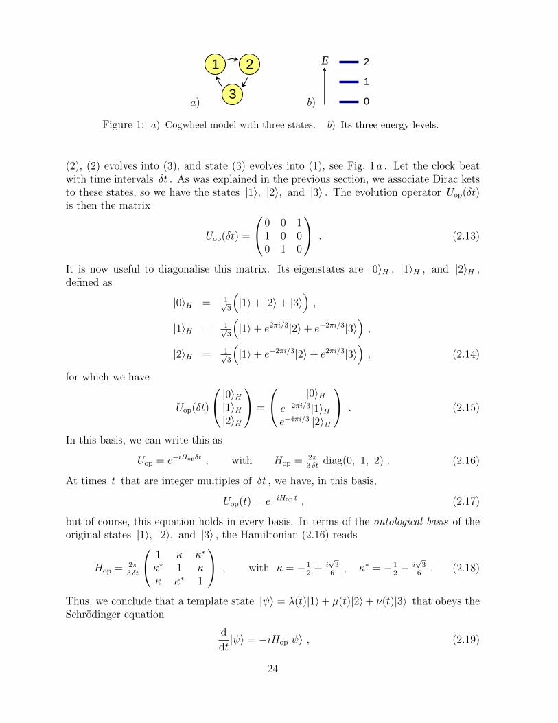
Figure 1: a) Cogwheel model with three states. b) Its three energy levels.

(2), (2) evolves into (3), and state (3) evolves into (1), see Fig. 1 a . Let the clock beatwith time intervals δt . As was explained in the previous section, we associate Dirac ketsto these states, so we have the states |1〉, |2〉, and |3〉 . The evolution operator Uop(δt)is then the matrix

Uop(δt) =

0 0 11 0 00 1 0

. (2.13)

It is now useful to diagonalise this matrix. Its eigenstates are |0〉H , |1〉H , and |2〉H ,defined as

|0〉H = 1√3

(|1〉+ |2〉+ |3〉

),

|1〉H = 1√3

(|1〉+ e2πi/3|2〉+ e−2πi/3|3〉

),

|2〉H = 1√3

(|1〉+ e−2πi/3|2〉+ e2πi/3|3〉

), (2.14)

for which we have

Uop(δt)

|0〉H|1〉H|2〉H

=

|0〉He−2πi/3|1〉He−4πi/3 |2〉H

. (2.15)

In this basis, we can write this as

Uop = e−iHopδt , with Hop = 2π3 δt

diag(0, 1, 2) . (2.16)

At times t that are integer multiples of δt , we have, in this basis,

Uop(t) = e−iHop t , (2.17)

but of course, this equation holds in every basis. In terms of the ontological basis of theoriginal states |1〉, |2〉, and |3〉 , the Hamiltonian (2.16) reads

Hop = 2π3 δt

1 κ κ∗

κ∗ 1 κκ κ∗ 1

, with κ = −12

+ i√

36, κ∗ = −1

2− i√

36. (2.18)

Thus, we conclude that a template state |ψ〉 = λ(t)|1〉+ µ(t)|2〉+ ν(t)|3〉 that obeys theSchrodinger equation

d

dt|ψ〉 = −iHop|ψ〉 , (2.19)

24

with the Hamiltonian (2.18), will be in the state described by the cogwheel model at alltimes t that are an integral multiple of δt . This is enough reason to claim that the“quantum” model obeying this Schrodinger equation is mathematically equivalent to ourdeterministic cogwheel model.

The fact that the equivalence only holds at integer multiples of δt is not a restriction.Imagine δt to be as small as the Planck time, 10−43 seconds (see chapter 6), then, ifany observable changes take place only on much larger time scales, deviations from theontological model will be unobservable. The fact the the ontological and the quantummodel coincide at all integer multiples of the time dt , is physically important. Note, thatthe original ontological model was not at all defined at non-integer time; we could simplydefine it to be described by the quantum model at non-integer times.

The eigenvalues of the Hamiltonian are 2π3 δt

n , with n = 0, 1, 2 , see Fig. 1 b . This isreminiscent of an atom with spin one that undergoes a Zeeman splitting due to a homo-geneous magnetic field. One may conclude that such an atom is actually a deterministicsystem with three states, or, a cogwheel, but only if the ‘proper’ basis has been identified.

The reader may remark that this is only true if, somehow, observations faster thanthe time scale δt are excluded. We can also rephrase this. To be precise, a Zeeman atomis a system that needs only 3 (or some other integer N ) states to characterise it. Theseare the states it is in at three (or N ) equally spaced moments in time. It returns to itselfafter the period T = Nδt .

2.2.1. Generalisations of the cogwheel model: cogwheels with N teeth

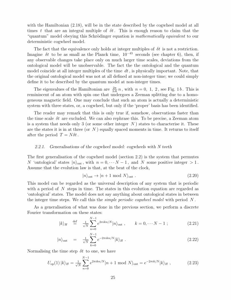
The first generalisation of the cogwheel model (section 2.2) is the system that permutesN ‘ontological’ states |n〉ont , with n = 0, · · ·N − 1 , and N some positive integer > 1 .Assume that the evolution law is that, at the beat of the clock,

|n〉ont → |n+ 1 mod N〉ont . (2.20)

This model can be regarded as the universal description of any system that is periodicwith a period of N steps in time. The states in this evolution equation are regarded as‘ontological’ states. The model does not say anything about ontological states in betweenthe integer time steps. We call this the simple periodic cogwheel model with period N .

As a generalisation of what was done in the previous section, we perform a discreteFourier transformation on these states:

|k〉Hdef= 1√

N

N−1∑n=0

e2πikn/N |n〉ont , k = 0, · · ·N − 1 ; (2.21)

|n〉ont = 1√N

N−1∑k=0

e−2πikn/N |k〉H . (2.22)

Normalising the time step δt to one, we have

Uop(1) |k〉H = 1√N

N−1∑n=0

e2πikn/N |n+ 1 mod N〉ont = e−2πik/N |k〉H , (2.23)

25

and we can conclude

Uop(1) = e−iHop ; Hop|k〉H = 2πkN|k〉H . (2.24)

This Hamiltonian is restricted to have eigenvalues in the interval [0, 2π) . where thenotation means that 0 is included while 2π is excluded. Actually, its definition impliesthat the Hamiltonian is periodic with period 2π , but in most cases we will treat it asbeing defined to be restricted to within the interval. The most interesting physical caseswill be those where the time interval is very small, for instance close to the Planck time,so that the highest eigenvalues of the Hamiltonian will be considered unimportant inpractice.

In the original, ontological basis, the matrix elements of the Hamiltonian are

ont〈m|Hop|n〉ont = 2πN2

N−1∑k=1

k e2πik(m−n)/N . (2.25)

This sum can we worked out further to yield

Hop = π

(1− 1

N

)− π

N

N−1∑n=1

(i

tan(πn/N)+ 1

)Uop(n) . (2.26)

Note that, unlike Eq. (2.8), this equation includes the corrections needed for the groundstate. For the other energy eigenstates, one can check that Eq. (2.26) agrees with Eq. (2.8).

For later use, Eqs. (2.26) and (2.8), without the ground state correction when U(t)|ψ〉 =|ψ〉 , can be generalised to the form

Hop = C − πi

T

tn<T∑tn>0

Uop(tn)

tan(πtn/T )

T→∞−→ C − i∑tn 6=0

Uop(tn)

tn, (2.27)

where C is a (large) constant, T is the period, and tn = n δt is the set of times wherethe operator U(tn) is required to have some definite value. We note that this is a sum,not an integral, so when the time values are very dense, the Hamiltonian tends to becomevery large. There seems to be no simple continuum limit. Nevertheless, in part II, we willattempt to construct a continuum limit, and see what happens (section 13).

Again, if we impose the Schrodinger equation ddt|ψ〉t = −iHop|ψ〉t and the boundary

condition |ψ〉t=0 = |n0〉ont , then this state obeys the deterministic evolution law (2.20)at integer times t . If we take superpositions of the states |n〉ont with the Born ruleinterpretation of the complex coefficients, then the Schrodinger equation still correctlydescribes the evolution of these Born probabilities.

It is of interest to note that the energy spectrum (2.24) is frequently encountered inphysics: it is the spectrum of an atom with total angular momentum J = 1

2(N − 1)

and magnetic moment µ in a weak magnetic field: the Zeeman atom. We observe that,after the discrete Fourier transformation (2.21), a Zeeman atom may be regarded as

26

the simplest deterministic system that hops from one state to the next in discrete timeintervals, visiting N states in total.

As in the Zeeman atom, we may consider the option of adding a finite, universalquantity δE to the Hamiltonian. It has the effect of rotating all states with the complexamplitude e−i δE after each time step. For a simple cogwheel, this might seem to be aninnocuous modification, with no effect on the physics, but below we shall see that theeffect of such an added constant might become quite significant later.

Note that, if we introduce any kind of perturbation on the Zeeman atom, causing theenergy levels to be split in intervals that are no longer equal, it will no longer look like acogwheel. Such systems will be a lot more difficult to describe in a deterministic theory;they must be seen as parts of a much more complex world.

2.2.2. The most general deterministic, time reversible, finite model

Figure 2: Example of a more generic finite, deterministic, time reversible model

Generalising the finite models discussed earlier in this chapter, consider now a modelwith a finite number of states, and an arbitrary time evolution law. Start with any state|n0〉ont , and follow how it evolves. After some finite number, say N0 , of time steps, thesystem will be back at |n0〉ont . However, not all states |n〉ont may have been reached.So, if we start with any of the remaining states, say |n1〉ont , then a new series of stateswill be reached, and the periodicity might be a different number, N1 . Continue until allexisting states of the model have been reached. We conclude that the most general modelwill be described as a set of simple periodic cogwheel models with varying periodicities,but all working with the same universal time step δt , which we could normalise to one;see Fig. 2.

Fig. 3 shows the energy levels of a simple periodic cogwheel model (left), a combinationof simple periodic cogwheel models (middle), and the most general deterministic, timereversible, finite model (right). Note that we now shifted the energy levels of all cogwheelsby different amounts δEi . This is allowed because the index i , telling us which cogwheel

27

a)

E

| 1 ⟩

| 0 ⟩

| N −1 ⟩

0

δE

δE +2π

b)

E

0 δEic)

E

0

Figure 3: a) Energy spectrum of the simple periodic cogwheel model. δE is anarbitrary energy shift. b) Energy spectrum of the model sketched in Fig. 2, whereseveral simple cogwheel models are combined. Each individual cogwheel i may beshifted by an arbitrary amount δEi . c) Taking these energy levels together we getthe spectrum of a generic finite model.

we are in, is a conserved quantity; therefore these shifts have no physical effect. Wedo observe the drastic consequences however when we combine the spectra into one, seeFig. 3 c .

Fig. 3 clearly shows that the energy spectrum of a finite discrete deterministic modelcan quickly become quite complex13. It raises the following question: given any kindof quantum system, whose energy spectrum can be computed. Would it be possible toidentify a deterministic model that mimics the quantum model? To what extent wouldone have to sacrifice locality when doing this? Are there classes of deterministic theoriesthat can be mapped on classes of quantum models? Which of these would be potentiallyinteresting?

3. Interpreting quantum mechanics

This book will not include an exhaustive discussion of all proposed interpretations of whatquantum mechanics actually is. Existing approaches have been described in excessivedetail in the literature [10][12][18][31][55], but we think they all contain weaknesses. Themost conservative attitude is the so-called Copenhagen Interpretation. It is also a verypragmatic one, and some mainstream researchers insist that it contains all we need toknow about quantum mechanics.

13It should be self-evident that the models displayed in the figures, and subsequently discussed, arejust simple examples; the real universe will be infinitely more complicated than these. One critic of ourwork was confused: “Why this model with 31 states? What’s so special about the number 31?” Nothing,of course, it is just an example to illustrate how the math works.

28

Yet it is the things that are not explained in the Copenhagen picture that often captureour attention. Below, we begin with indicating how the cellular Automaton interpretationwill address some of these questions.

3.1. The Copenhagen Doctrine

It must have been a very exciting period of early modern science, when researchers be-gan to understand how to handle quantum mechanics, in the late 1920s and subsequentyears. [44] The first coherent picture of how one should think of quantum mechanics, iswhat we now shall call the Copenhagen Doctrine. In the early days, physicists were stillstruggling with the equations and the technical difficulties. Today, we know precisely howto handle all these, so that now we can rephrase the original starting points much moreaccurately. Originally, quantum mechanics was formulated in terms of wave functions,with which one referred to the states electrons are in; ignoring spin for a moment, theywere the functions ψ(~x, t) = 〈~x |ψ(t)〉 . Now, we may still use the words ‘wave function’when we really mean to talk of ket states in more general terms.

Leaving aside who said exactly what in the 1920s, here are the main points of whatone might call the Copenhagen Doctrine. Somewhat anachronistically, we employ Dirac’snotation:

A system is completely described by its ‘wave function’ |ψ(t)〉 , which is anelement of Hilbert space, and any basis in Hilbert space can be used for itsdescription. This wave function obeys a linear first order differential equationin time, to be referred to as Schrodinger’s equation, of which the exact formcan be determined by repeated experiments.A measurement can be made using any observable O that one might wantto choose (observables are hermitean operators in Hilbert space). The theorythen predicts the average measured value of O , after many repetitions of theexperiment, to be

〈O〉 = 〈ψ(t)|O|ψ(t)〉 . (3.1)

As soon as the measurement is made, the wave function of the system collapsesto a state in the subspace of Hilbert space that is an eigenstate of the observ-able O , or a probabilistic distribution of eigenstates, according to Eq. (3.1).When two observables O1 and O2 do not commute, they cannot both be mea-sured accurately. The commutator [O1, O2] indicates how large the productof the ‘uncertainties’ δO1 and δO2 should be expected to be.The measuring device itself must be regarded as a classical object, and forlarge systems the quantum mechanical measurement approaches closely theclassical description.

Implicitly included in Eq. (3.1) is the element of probability. If we expand the wavefunction |ψ〉 into eigenstates |ϕ〉 of an observable O , then we find that the probability

29

that the experiment on |ψ〉 actually gives as a result that the eigenvalue of the state |ϕ〉is found, will be given by P = |〈ϕ|ψ〉|2 . This is referred to as Born’s probability rule [2].

We note that the wave function may not be given any ontological significance. Theexistence of a ‘pilot wave’ is not demanded; one cannot actually measure 〈ϕ|ψ〉 itself;only by repeated experiments, one can measure the probabilities, with intrinsic margins oferror. We say that the wave function, or more precisely, the amplitudes, are psi-epistemicrather than psi-ontic.

An important element in the Copenhagen interpretation is that one may only askwhat the outcome of an experiment will be. In particular, it is forbidden to ask: whatis it that is actually happening? It is exactly the latter question that sparks endlessdiscussions; the important point made by the Copenhagen group is that such questionsare unnecessary. If one knows the Schrodinger equation, one knows everything needed topredict the outcomes of an experiment, no further questions should be asked.

This is a strong point of the Copenhagen doctrine, but it also yields severe limitations.If we know the Schrodinger equation, we know everything there is to be known.

But what if we do not yet know the Schrodinger equation? How does one arrive atthe correct equation? In particular, how do we arrive at the correct Hamiltonian if thegravitational force is involved?

Gravity has been a major focus point of the last 30 years and more, in elementaryparticle theory and the theory of space and time. Numerous wild guesses have been made.In particular, (super)string theory has made huge advances. Yet no convincing model thatunifies gravity with the other forces has been constructed; models proposed so-far havenot been able to explain, let alone predict, the values of the fundamental constants ofNature, including the masses of many fundamental particles, the fine structure constant,and the cosmological constant. And here it is, according to the author’s opinion, wherewe do have to ask: What is it, or what could it be, that is actually going on?

One strong feature of the Copenhagen approach to quantum theory was that it wasalso clearly shown how a Schrodinger equation can be obtained if the classical limit isknown:

If a classical system is described by the (continuous) Hamilton equations, thismeans that we have classical variables pi and qi , for which one can definePoisson brackets : any pair of observables A(~q, ~p ) and B(~q, ~p ) , allow for theconstruction of an observable variable called A,B , defined by

A,B ≡∑i

(∂A∂qi

∂B

∂pi− ∂A

∂pi

∂B

∂qi

), (3.2)

in particular:

qi, pj = −pi, qj = δij , qi, qj = pi, pj = 0 . (3.3)

A quantum theory is obtained, if we replace the Poisson brackets by commu-tators, which involves a factor i and a new constant of Nature, ~ . Basically:

[A,B]→ i~A,B . (3.4)

30

In the limit ~ → 0 , this quantum theory reproduces the classical system. This verypowerful procedure allows us, more often than not, to bypass the question “what is go-ing on?”. We have a theory, we know where to search for the appropriate Schrodingerequation, and we know how to recover the classical limit.

Unfortunately, in the case of the gravitational force, this ‘trick’ is not good enough togive us ‘quantum gravity’. The problem with gravity is not just that the gravitational forceappears not to be renormalizable, or that it is difficult to define the quantum versions ofspace- and time coordinates, and the physical aspects of non-trivial space-time topologies;some authors attempt to address these problems as merely technical ones, which can behandled by using some tricks. The real problem is that space-time curvature runs out ofcontrol at the Planck scale. We will be forced to turn to a different book keeping systemfor Nature’s physical degrees of freedom there.

A promising approach was to employ local conformal symmetry [89] as a more funda-mental principle than usually thought; this could be a way to make distance and timescales relative, so that what was dubbed as ‘small distances’ ceases to have an absolutemeaning. The theory is recapitulated in Appendix B. It does need further polishing,and it too could eventually require a Cellular Automaton interpretation of the quantumfeatures that it will have to include.

3.2. The Einsteinian view

This section is called “The Einsteinian view’, rather than ‘Einstein’s view’, because wedo not want to go into a discussion of what it actually was that Einstein thought. It iswell-known that Einstein was uncomfortable with the Copenhagen Doctrine. The notionthat there might be ways to rephrase things such that all phenomena in the universe arecontrolled by equations that leave nothing to chance, will now be referred to as the Ein-steinian view. We do ask further questions, such as Can quantum-mechanical descriptionof physical reality be considered complete? [6], or, does the theory tell us everything wemight want to know about what is going on?

In the Einstein-Podolsky-Rosen discussion of a Gedanken experiment, two particles(photons, for instance), are created in a state

x1 − x2 = 0 , p1 + p2 = 0 . (3.5)

Since [x1−x2, p1 +p2] = i− i = 0 , both equations in (3.5) can be simultaneously sharplyimposed.

What bothered Einstein, Podolsky and Rosen was that, long after the two particlesceased to interact, an observer of particle # 2 might decide either to measure its momen-tum p2 , after which we know for sure the momentum p1 of particle # 1, or its positionx2 , after which we would know for sure the position x1 of particle #1. How can sucha particle be described by a quantum mechanical wave function at all? Apparently, themeasurement at particle # 2 affected the state of particle #1, but how could that havehappened?

31

In modern quantum terminology, however, we would have said that the measurementsproposed in this Gedanken experiment would have disturbed the wave function of theentangled particles. The measurements on particle # 2 affects the probability distributionsfor particle # 1, which in no way should be considered as the effect of a spooky signalfrom one system to the other.

In any case, even Einstein, Podolsky and Rosen had no difficulty in computing thequantum mechanical probabilities for the outcomes of the measurements, so that, inprinciple, quantum mechanics emerged unharmed out of this sequence of arguments.

It is much more difficult to describe the two EPR photons in a classical model. Suchquestions will be the topic of section 3.6.

Einstein had difficulties with the relativistic invariance of quantum mechanics (“doesthe spooky information transmitted by these particles go faster than light?”). These,however, are now seen as technical difficulties that have been resolved. It may be consid-ered part of Copenhagen’s Doctrine, that the transmission of information over a distancecan only take place, if we can identify operators A at space-time point x1 and operatorsB at space-time point x2 that do not commute: [A,B] 6= 0 . We now understand that, inelementary particle theory, all space-like separated observables mutually commute, whichprecludes any signalling faster than light. It is a built-in feature of the Standard Model,to which it actually owes much of its success.

So, with the technical difficulties out of the way, we are left with the more essentialEinsteinian objections against the Copenhagen doctrine for quantum mechanics: it is aprobabilistic theory that does not tell us what actually is going on. It is sometimes evensuggested that we have to put our “classical” sense of logic on hold. Others deny that:“Keep remembering what you should never ask, while reshaping your sense of logic, andeverything will be fine.” According to the present author, the Einstein-Bohr debate is notover. A theory must be found that does not force us to redefine any aspect of classical,logical reasoning.

What Einstein and Bohr did seem to agree about is the importance of the role of anobserver. Indeed, this was the important lesson learned in the 20th century: if somethingcannot be observed, it may not be a well-defined concept – it may even not exist at all. Wehave to limit ourselves to observable features of a theory. It is an important ingredientof our present work that we propose to part from this doctrine, at least to some extent:Things that are not directly observable may still exist and as such play a decisive rolein the observable properties of an object. They may also help us to construct realisticmodels of the world.

Indeed, there are big problems with the dictum that everything we talk about must beobservable. While observing microscopic objects, an observer may disturb them, even ina classical theory; moreover, in gravity theories, observers may carry gravitational fieldsthat disturb the system they are looking at, so we cannot afford to make an observerinfinitely heavy (carrying large bags full of “data”, whose sheer weight gravitationallydisturbs the environment), but also not infinitely light (light particles do not transmitlarge amounts of data at all), while, if the mass of an observer would be “somewhere in

32

between”, this could entail that our theory will be inaccurate from its very inception.

An interesting blow was given to the doctrine that observability should be central,when quark theory was proposed. Quarks cannot be isolated to be observed individu-ally, and for that reason the idea that quarks would be physical particles was attacked.Fortunately, in this case the theoretical coherence of the evidence in favour of the quarksbecame so overwhelming, and experimental methods for observing them, even while theyare not entirely separated, improved so much, that all doubts evaporated.

In short, the Cellular Automaton Interpretation tells us to return to classical logic andbuild models. These models describe the evolution of large sets of data, which eventuallymay bring about classical phenomena that we can observe. The fact that these datathemselves cannot be directly observed, and that our experiments will provide nothingbut statistical information, including fluctuations and uncertainties, can be fully explainedwithin the settings of the models; if the observer takes no longer part in the definitionof physical degrees of freedom and their values, then his or her limited abilities will nolonger stand in the way of accurate formalisms.

We suspect that this view is closer to Einstein’s than it can be to Bohr, but, in asense, neither of them would fully agree. We do not claim the wisdom that our view isobviously superior, but rather advocate that one should try to follow such paths, andlearn from our successes and failures.

3.3. Notions not admitted in the C.A.I.

It is often attempted to attach a physical meaning to the wave function beyond what itis according to Copenhagen. Could it have an ontological significance as a ‘pilot wavefunction’ [3][10]? It should be clear from nearly every page of this book that we do notwish to attach any ontological meaning to the wave function, if we are using it as atemplate.

In an ontological description of our universe, in terms of its ontological basis, thereare only two values a wave function can take: 1 and 0. A state is actually realised whenthe wave function is 1, and it does not describe our world when the wave function is zero.It is only this ‘universal wave function’, that for that reason may be called ontological.

It is only for mathematical reasons that one might subsequently want to equip thiswave function with a phase, eiϕ . In the ontological basis, this phase ϕ has no physicalmeaning at all, but as soon as one considers operators, including the time-evolution op-erator U(t) , and therefore also the Hamiltonian, these phases have to be chosen. Froma physical point of view, any phase is as good as any other, but for keeping the mathe-matical complexity under control, precise definitions of these phases is crucial. One canthen perform the unitary transformations to any of the basis choices usually employedin physics. The template states subsequently introduced, all come with precisely definedphases.

A semantic complication is caused as soon as we apply second quantisation. Wherea single particle state is described by a wave function, the second-quantized version of

33

the theory sometimes replaces this by an operator field. Its physical meaning is thencompletely different. Operator fields are usually not ontological since they are superim-posables rather than beables (see subsection 2.1.1), but in principle they could be; wavefunctions, in contrast, are elements of Hilbert space and as such should not be confusedwith operators, let alone beable operators.

How exactly to phrase the so-called ‘Many World Interpretation’ [12] of quantum me-chanics, is not always agreed upon [21]. When doing ordinary physics with atoms andelementary particles, this interpretation may well fulfil the basic needs of a researcher,but from what has been learned in this book it should be obvious that our theory con-trasts strongly with such ideas. There is only one single world that is being selected outin our theory as being ‘the real world’, while all others simply are not realised.

The reader may have noticed that the topic in this book is being referred to alternatelyas a ‘theory’ and as an ‘interpretation’. The theory we describe consists not only of theassumption that an ontological basis exists, but also that it can be derived, so as to providean ontological description of our universe. It suggests pathways to pin down the nature ofthis ontological basis. When we talk of an interpretation, this means that, even if we findit hard or impossible to identify the ontological basis, the mere assumption that one mightexist suffices to help us understand what the quantum mechanical expressions normallyemployed in physics, are actually standing for, and how a physical reality underlying themcan be imagined.

3.4. The collapsing wave function and Schrodinger’s cat

The following ingredient in the Copenhagen interpretation, section 3.1, is often the subjectof discussions:

As soon as an observable O is measured, the wave function of the systemcollapses to a state in the subspace of Hilbert space that is an eigenstate of theobservable O , or a probabilistic distribution of eigenstates.

This is referred to as the “collapse of the wave function”. It appears as if the action of themeasurement itself causes the wave function to attain its new form. The question thenasked is what physical process is associated to that.

Again, the official reply according to the Copenhagen doctrine is that this questionshould not be asked. Do the calculation and check your result with the experiments. How-ever, there appears to be a contradiction, and this is illustrated by Erwin Schrodinger’sGedanken experiment with a cat. [8] The experiment is summarised as follows:

In a sealed box, one performs a typical quantum experiment. It could be aStern Gerlach experiment where a spin 1

2particle with spin up is sent through

an inhomogeneous magnetic field that splits the wave function according tothe values of the spin in the y direction, or it could be a radioactive atomthat has probability 1

2to decay within a certain time. In any case, the wave

34

function is well specified at t = 0 , while at t = 1 it is in a superpositionof two states, which are sent to a detector that determines which of the twostates is realised. It is expected that the wave function ‘collapses’ into one ofthe two possible final states.The box also contains a live cat (and air for the cat to breathe). Dependingon the outcome of the measurement, a capsule with poison is broken, or keptintact. The cat dies when one state is found, and otherwise the cat stays alive.At the end of the experiment, we open the box and inspect the cat.

Clearly, the probability that we find a dead cat is about 12

, and otherwise we find a livecat. However, we could also regard the experiment from a microscopic point of view. Theinitial state was a pure quantum state. The final state is a superposition. Should the cat,together with the other remains of the experiment, upon opening the box, not be foundin a superimposed state: dead and alive?

The collapse axiom tells us that the state should be ‘dead cat’ or ‘live cat’, whereas thefirst parts of our description of the quantum mechanical states of Hilbert space, clearlydictates that if two states, |ψ1〉 and |ψ2〉 are possible in a quantum system, then wecan also have α|ψ1〉 + β|ψ2〉 . According to Schrodinger’s equation, this superposition ofstates always evolves into a superposition of the final states. The collapse seems to violateSchrodinger’s equation. Something is not quite right.

An answer that several investigators have studied [33], is that, apparently, Schrodinger’sequation is only an approximation, and that tiny non-linear ‘correction terms’ bring aboutthe collapse [38][53][54]. One of the problems with this is that observations can be madeat quite different scales of space, time, energy and mass. How big should the putativecorrection terms be? Secondly, how do the correction terms know in advance which mea-surements we are planning to perform?

This, we believe, is where the cellular automaton interpretation of quantum mechanicswill come to the rescue. It is formulated using no wave function at all, but there areontological states instead. It ends up with just one wave function, taking the value 1 ifwe have a state the universe is in, and 0 if that state is not realised. There are no otherwave functions, no superposition.

How this explains the collapse phenomenon will be explained in chapter 4. In sum-mary: quantum mechanics is not the basic theory but a tool to solve the mathematicalequations. This tool works just as well for superimposed states (the templates) as for theontological states, but they are not the same thing. The dead cat is in an ontological stateand so is the live one. The superimposed cat solves the equations mathematically in aperfectly acceptable way, but it does not describe a state that can occur in the real world.We postpone the precise explanation to chapter 4. It will sound very odd to physicistswho have grown up with standard quantum mechanics, but it does provide the logicalsolution to the Schrodinger cat paradox.14

14Critical readers will say: Of course, this theory isn’t quantum mechanics, so it doesn’t share any ofits problems. True, but our theory is supposed to generate quantum mechanics, without generating itsassociated problems.

35

One may ask what this may imply when we have transformations between ontologicalstates and template states. Our experiences tell us that all template states that aresuperpositions α|ψ1〉+ β|ψ2〉 of ontological states, may serve as suitable approximationsdescribing probabilistic situations in the real world. How can it be that, sometimes, theydo seem to be ontological? The most likely response to that will be that the transformationdoes not always have to be entirely local, but in practice may involve many spectatorstates in the environment. What we can be sure of is that all ontological states form anorthonormal set. So, whenever we use α|ψ1〉 + β|ψ2〉 to describe an ontological state,there must be other wave functions in the environment which must be chosen differentlyfor any distinct pair α and β , such that the entire set that we use to describe physicalsituations are always orthonormal.

This should be taken in mind in the next sections where we comment on the Alice andBob Gedanken experiments.

3.5. Decoherence and Born’s probability axiom

The cellular automaton interpretation does away with one somewhat murky ingredientof the more standard interpretation schemes: the role of ‘decoherence’. It is the argu-ment often employed to explain why macroscopic systems are never seen in a quantumsuperposition. Let |ψ1〉 and |ψ2〉 be two states a classical system can be in, such as a catbeing dead and a cat being alive. According to Copenhagen, in its pristine form, quantummechanics would predict the possibility of a third state, |ψ3〉 = α|ψ1〉 + β|ψ2〉 , where αand β can be any pair of complex numbers with |α|2 + |β|2 = 1 .

Indeed, it seems almost inevitable that a system that can evolve into state |ψ1〉 orinto state |ψ2〉 , should also allow for states that evolve into |ψ3〉 . Why do we not observesuch states? The only thing we do observe is a situation whose probability of being in|ψ1〉 might be |α|2 and the probability to be in |ψ2〉 is |β|2 . But that is not the sameas state |ψ3〉 .

The argument is that, somehow, the state |ψ3〉 is unstable. According to Copenhagen,the probability of a state |ψ〉 to be in state |ψ3〉 is

P3 = |〈ψ3|ψ〉|2 = |α|2|〈ψ1|ψ〉|2 + |β|2|〈ψ2|ψ〉|2 + 2Re(α∗β〈ψ|ψ1〉〈ψ2|ψ〉

). (3.6)

The last term here is the interference term. It distinguishes the real quantum theory fromclassical theories. Now it is said that, if |ψ1〉 and |ψ2〉 become classical, they cannot stayimmune for interactions with the environment. In the presence of such interactions, theenergies of |ψ1〉 and |ψ2〉 will not exactly match, and consequently, the interference term,will oscillate badly. This term might then be seen to average out to zero. The first twoterms are just the probabilities to have either |ψ1〉 or |ψ2〉 , which would be the classicalprobabilities.

If indeed the last term becomes unobservable, we say that the two states deco-here [45][54], so that the interference term should be replaced by zero. The questionis, if we include the environment in our description, the energies should still be exactly

36

conserved, and there is no rapid oscillation. Is it legal to say nevertheless that the inter-ference term will disappear? Note that its absolute value on average does remain large.

The CAI will give a much more direct answer: if states |ψ1〉 and |ψ2〉 are classical,then they are ontological states. State |ψ3〉 will then not be an ontological state, andthe states of the real universe, describing what happens if an actual experiment is carriedout, never include state |ψ3〉 . It is merely a template, useful for calculations, but notdescribing reality. What it may describe is a situation where, from the very start, thecoefficients α and β were declared to represent probabilities.

Copenhagen quantum mechanics contains an apparently irreducible axiom: the prob-ability that a state |ψ〉 is found to agree with the properties of another state |ϕ〉 , mustbe given by

P = |〈ϕ|ψ〉|2 . (3.7)

This is the famous Born rule [2]. What is the physical origin of this axiom?

Note, that Born did not have much of a choice. The completeness theorem of linearalgebra implies that the eigenstates |ϕ〉 of an hermitean operator span the entire Hilbertspace, and therefore,∑

ϕ

|ϕ〉〈ϕ| = I ;∑ϕ

|〈ϕ|ψ〉|2 =∑ϕ

〈ψ|ϕ〉〈ϕ|ψ〉 = 〈ψ|ψ〉 = 1 , (3.8)

where I stands for the identity operator. If Born would have chosen any other expressionto represent probabilities, according to Gleason’s theorem [13], they would not have addedup to one. The expression (3.7) turns out to be ideally suited to serve as a probability.

Yet this is a separate axiom, and the question why it works so well is not misplaced.In a hidden variable theory, probabilities may have a different origin. The most naturalexplanation as to why some states are more probable than others may be traced totheir initial states much earlier in time. One can ask which initial states may havelead to a state seen at present, and how probable these may have been. There may benumerous answers to that question. One now could attempt to estimate their combinedprobabilities. The relative probabilities of some given observed final states could then berelated to the ratios of the numbers found. Our question then is, can we explain whetherand how the expression (3.7) is related to these numbers? This discussion is continued insubsection 3.6.1 and in section 4.3.

3.6. Bell’s theorem, Bell’s inequalities and the CHSH inequality.

One of the main reasons why ‘hidden variable’ theories are usually dismissed, and em-phatically so when the theory obeys local equations, is the apparent difficulty in suchtheories to represent entangled quantum states. Just because the De Broglie-Bohm the-ory (not further discussed here) is intrinsically non-local, it is generally concluded thatall hidden variable theories are either non-local or unable to reproduce quantum featuresat all. When J.S. Bell was investigating the possibility of hidden variable theories, he hit

37

upon the same difficulties, upon which he attempted to prove that local hidden variabletheories are impossible.

As before, we do not intend to follow precisely the historical development of Bell’stheory [31], but limit ourselves to a summary of the most modern formulation of theprinciples. Bell designed a Gedanken experiment, and at the heart of it is a pair ofquantum-entangled particles. They could be spin- 1

2particles, which each can be in

just two quantum states described by the Pauli matrices (1.7), or alternatively spin 1photons. There are a few subtle differences between these two cases, although these arenot essential to the argument. The first is that the two orthonormal states for photons arethe ones where they are polarised horizontally or vertically, while the two spin- 1

2states

are polarised up or down. Indeed, quite generally when polarised particles are discussed,the angles for the photons are handled as being half the angles for spin- 1

2particles.

The second difference concerns the entangled state, which in both cases has totalspin 0. For spin- 1

2, this means that (~σ1 + ~σ2)|ψ〉 = 0 , where ~σ are the Pauli matrices,

Eqs. (1.7), so that

|ψ〉 = 1√2(| ↑↓〉 − | ↓↑〉) , (3.9)

which means that the two electrons are polarised in opposite directions.

For spin 1, this is different. Let us have these photons move in the ±z -direction.Defining A± = 1√

2(Ax ± iAy) as the operators that create or annihilate one unit of spin

in the z -direction, and taking into account that photons are bosons, the 2 photon statewith zero spin in the z -direction is

|ψ〉 = 1√2(A

(1)+ A

(2)− + A

(1)− A

(2)+ ) | 〉 = 1√

2|z, −z〉+ 1√

2| − z, z〉 , (3.10)

and since helicity is spin in the direction of motion, while the photons go in oppositedirections, we can rewrite this state as

|ψ〉 = 1√2( |+ +〉+ | − −〉 ) , (3.11)

where ± denote the helicities. Alternatively one can use the operators Ax and Ay toindicate the creators of linearly polarised photons, and then we have

|ψ〉 = 1√2(A(1)

x A(2)x + A(1)

y A(2)y ) | 〉 = 1√

2( |xx〉+ |yy〉 ) . (3.12)

Thus, the two photons are linearly polarised in the same direction.

Since the experiment is mostly done with photons, we will henceforth describe theentangled photon state.

The Bell experiment is now illustrated in Fig. 4. At the point S , an atom ε isprepared to be in an unstable J = 0 state at t = t1 , such that it can decay only into another J = 0 state, by simultaneously emitting two photons such that ∆J = 0 , and thetwo photons, α and β , must therefore be in the entangled Stot = 0 state, at t = t2 .

After having travelled for a long time, at t = t3 , photon α is detected by observer A(Alice), and photon β is detected by B (Bob). Ideally, the observers use a polarisation

38

x

tBA

SQA QB

`_

¡

cc

ba

t = t0

t = t1

t = t2

t = t3

t = t4

BobAlice

Figure 4: A bell-type experiment. Space runs horizontally, time vertically. Singlelines denote single bits or qubits travelling; widened lines denote classical informa-tion carried by millions of bits. Light travels along 45 , as indicated by the lightcone on the right. Meaning of the variables: see text.

filter oriented at an angle a (Alice) and b (Bob). If the photon is transmitted by thefilter, it is polarised in the direction of the polarisation filter’s angle, if it is reflected, itspolarisation was orthogonal to this angle. At both sides of the filter there is a detector, soboth Alice and Bob observe that one of their two detectors gives a signal. We call Alice’ssignal A = +1 if the photon passed the filter, and A = −1 if it is reflected. Bob’s signalB is defined the same way.

According to quantum theory, if A = 1 , Alice’s photon is polarised in the directiona , so Bob’s photon must also be polarised in that direction, and the intensity of thelight going through Bob’s filter will be cos2(a − b) . Therefore, according to quantumtheory, the probability that B = 1 is cos2(a− b) . The probability that B = −1 is thensin2(a− b) , and the same reasoning can be set up if A = −1 . The expectation value ofthe product AB is thus found to be

〈AB 〉 = cos2(a− b)− sin2(a− b) = cos 2(a− b) , (3.13)

according to quantum mechanics.

In fact, these correlation functions can now be checked experimentally. Beautifulexperiments [32] confirmed that correlations can come close to Eq. (3.13).

The point made by Bell is that it seems to be impossible to reproduce this strongcorrelation between the findings A and B in any theory where classical information ispassed on from the atom ε to Alice (A) and Bob (B). All one needs to assume is that theatom emits a signal to Alice and one to Bob, regarding the polarisation of the photonsemitted. It could be the information that both photons α and β are polarised in directionc . Since this information is emitted long before either Alice or Bob decided how to orienttheir polarisation filters, it is obvious that the signals in α and β should not depend onthat. Alice and Bob are free to choose their polarisers.

39

The correlations then directly lead to a contradiction, regardless the nature of theclassical signals used. The contradiction is arrived at as follows. Consider two choicesthat Alice can make: the angles a and a ′ . Similarly, Bob can choose between anglesb and b ′ . Whatever the signal is that the photons carry along, it should entail anexpectation value for the four observations that can be made: Alice observes A or A′ inthe two cases, and Bob observes B or B′ . If both Alice and Bob make large numbersof observations, every time using either one of their two options, they can compare notesafterwards, and measure the averages of AB , A′B , AB′ , and A′B′ . They calculatethe value of

S = 〈AB〉+ 〈A′B〉+ 〈AB′ 〉 − 〈A′B′ 〉 , (3.14)

and see how it depends on the polarisation angles a and b .

Now suppose we assume that, every time photons are emitted, they have well-definedvalues for A, A′, B , and B′ . Whatever the signals are that are carried by the photons,at each measurement these four terms will take the values ±1 , but they can never allcontribute to the quantity S with the same sign (because of the one minus sign in (3.14)).Because of this, it is easy to see that S is always ±2 , and its average value will thereforeobey:

|〈S〉| ≤ 2 ; (3.15)

this modern version of Bell’s original observation is called the Clauser-Horne-Shimony-Holt (CHSH) inequality [20]. However, if we choose the angles

a = 22.5 , a′ = −22.5 , b = 0 , b′ = 45 , (3.16)

then, according to Eq. (3.13), quantum mechanics gives for the expectation value

S = 3 cos(45)− cos 135 = 2√

2 > 2 . (3.17)

How can this be? Apparently, quantum mechanics does not give explicit values ±1 forthe measurements of A and A′ ; it only gives a value to the quantity actually measured,which in each case is either A or A′ and also either B or B′ . If Alice measures A ,she cannot also measure A′ because the operator for A′ does not commute with A ; thepolarisers differ by an angle of 45 , and a photon polarised along one of these anglesis a quantum superposition of a photon polarised along the other angle and a photonpolarised orthogonally to that. So the quantum outcome is completely in accordancewith the Copenhagen prescriptions, but it seems that it cannot be realised in a localhidden variable theory.

We say that, if A is actually measured, the measurement of A′ is counterfactual,which means that we imagine measuring A′ but we cannot actually do it, just as weare unable to measure position if we already found out what exactly the momentum ofa particle is. If two observables do not commute, one can measure one of them, but themeasurement of the other is counterfactual.

40

Indeed, in the arguments used, it was assumed that the hidden variable theory shouldallow an observer actually to carry out counterfactual measurements. This is called defi-niteness. Local hidden variable theories that allow for counterfactual observations are saidto have local definiteness. Quantum mechanics forbids local counterfactual definiteness.

However, to use the word ‘definiteness’, or ‘realism’, for the possibility to performcounterfactual observations is not very accurate. ‘realism’ should mean that there isactually something happening, not a superposition of things; something is happening forsure, while something else is not happening. That is not the same thing as saying thatboth Alice and Bob at all times can choose to modify their polarisation angles, withoutallowing for any modification at other places [63].

It is here that the notion of “free will” is introduced [58][59], again, in an imprecisemanner15. The real extra assumption made by Bell, and more or less tacitly by manyof his followers, is that both Alice and Bob should have the “free will” to modify theirsettings at any moment, without having to consult the settings at the system S thatproduces an unstable atom. If this were allowed to happen in a hidden variable theory,we would get local counterfactual definiteness, which was ruled out.

The essence of the argument that now follows has indeed been raised before. Theformulation by C.H. Brans [40] is basically correct, but we add an extra twist, somethingto be called the ‘ontology conservation law’, in order to indicate why violation of Bell’stheorem does not require ‘absurd physics’.

How can we deny Alice and/or Bob their free will? Well, precisely in a deterministichidden variable theory, Alice and Bob can only change their minds about the setting oftheir polarisers, if their brains follow different laws than they did before, and, like it ornot, Alice’s and Bob’s actions are determined by laws of physics [84], even if these areonly local laws. Their decisions, logically, have their roots in the distant past, going backall the way to the Big Bang. So why should we believe that they can do counterfactualobservations?

The way this argument is usually countered is that the correlations between the pho-tons c from the decaying atom and the settings a and b chosen by Alice and Bob haveto be amazingly strong. A gigantically complex algorithm could make Alice an Bob taketheir decisions, and yet the decaying atom, long before Alice and Bob applied this algo-rithm, knew about the result. This is called ‘conspiracy’, and conspiracy is said to be“disgusting”. “One could better stop doing physics than believe such a weird thing”, iswhat several investigators quipped.

In subsections 3.6.2, 5.7.3 and 10.3.3, we go to the core of this issue.

15One can certainly attempt to define ‘free will’ in terms of sound mathematical physics. See Part II,subsection 10.3.4.

41

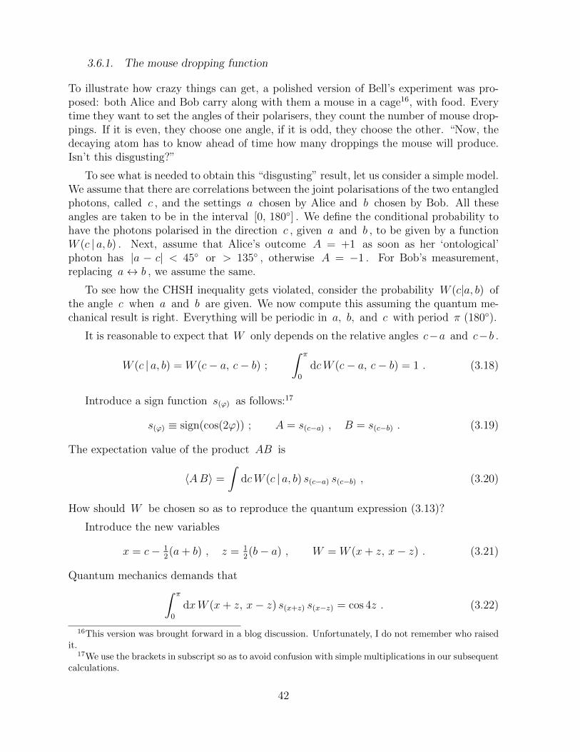
3.6.1. The mouse dropping function

To illustrate how crazy things can get, a polished version of Bell’s experiment was pro-posed: both Alice and Bob carry along with them a mouse in a cage16, with food. Everytime they want to set the angles of their polarisers, they count the number of mouse drop-pings. If it is even, they choose one angle, if it is odd, they choose the other. “Now, thedecaying atom has to know ahead of time how many droppings the mouse will produce.Isn’t this disgusting?”

To see what is needed to obtain this “disgusting” result, let us consider a simple model.We assume that there are correlations between the joint polarisations of the two entangledphotons, called c , and the settings a chosen by Alice and b chosen by Bob. All theseangles are taken to be in the interval [0, 180] . We define the conditional probability tohave the photons polarised in the direction c , given a and b , to be given by a functionW (c | a, b) . Next, assume that Alice’s outcome A = +1 as soon as her ‘ontological’photon has |a − c| < 45 or > 135 , otherwise A = −1 . For Bob’s measurement,replacing a↔ b , we assume the same.

To see how the CHSH inequality gets violated, consider the probability W (c|a, b) ofthe angle c when a and b are given. We now compute this assuming the quantum me-chanical result is right. Everything will be periodic in a, b, and c with period π (180).

It is reasonable to expect that W only depends on the relative angles c−a and c−b .

W (c | a, b) = W (c− a, c− b) ;

∫ π

0

dcW (c− a, c− b) = 1 . (3.18)

Introduce a sign function s(ϕ) as follows:17

s(ϕ) ≡ sign(cos(2ϕ)) ; A = s(c−a) , B = s(c−b) . (3.19)

The expectation value of the product AB is

〈AB〉 =

∫dcW (c | a, b) s(c−a) s(c−b) , (3.20)

How should W be chosen so as to reproduce the quantum expression (3.13)?

Introduce the new variables

x = c− 12(a+ b) , z = 1

2(b− a) , W = W (x+ z, x− z) . (3.21)

Quantum mechanics demands that∫ π

0

dxW (x+ z, x− z) s(x+z) s(x−z) = cos 4z . (3.22)

16This version was brought forward in a blog discussion. Unfortunately, I do not remember who raisedit.

17We use the brackets in subscript so as to avoid confusion with simple multiplications in our subsequentcalculations.

42

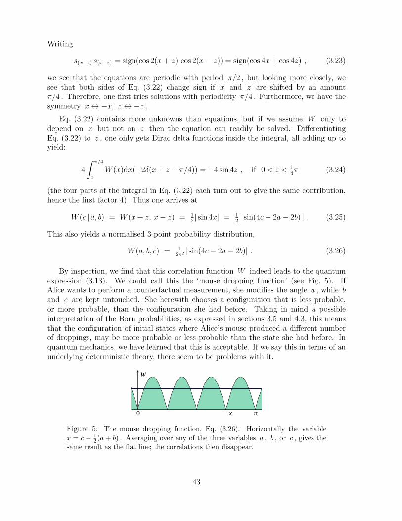
Writing

s(x+z) s(x−z) = sign(cos 2(x+ z) cos 2(x− z)) = sign(cos 4x+ cos 4z) , (3.23)

we see that the equations are periodic with period π/2 , but looking more closely, wesee that both sides of Eq. (3.22) change sign if x and z are shifted by an amountπ/4 . Therefore, one first tries solutions with periodicity π/4 . Furthermore, we have thesymmetry x↔ −x, z ↔ −z .

Eq. (3.22) contains more unknowns than equations, but if we assume W only todepend on x but not on z then the equation can readily be solved. DifferentiatingEq. (3.22) to z , one only gets Dirac delta functions inside the integral, all adding up toyield:

4

∫ π/4

0

W (x)dx(−2δ(x+ z − π/4)) = −4 sin 4z , if 0 < z < 14π (3.24)

(the four parts of the integral in Eq. (3.22) each turn out to give the same contribution,hence the first factor 4). Thus one arrives at

W (c | a, b) = W (x+ z, x− z) = 12| sin 4x| = 1

2| sin(4c− 2a− 2b) | . (3.25)

This also yields a normalised 3-point probability distribution,

W (a, b, c) = 12π2 | sin(4c− 2a− 2b)| . (3.26)

By inspection, we find that this correlation function W indeed leads to the quantumexpression (3.13). We could call this the ‘mouse dropping function’ (see Fig. 5). IfAlice wants to perform a counterfactual measurement, she modifies the angle a , while band c are kept untouched. She herewith chooses a configuration that is less probable,or more probable, than the configuration she had before. Taking in mind a possibleinterpretation of the Born probabilities, as expressed in sections 3.5 and 4.3, this meansthat the configuration of initial states where Alice’s mouse produced a different numberof droppings, may be more probable or less probable than the state she had before. Inquantum mechanics, we have learned that this is acceptable. If we say this in terms of anunderlying deterministic theory, there seem to be problems with it.

W

x π0

Figure 5: The mouse dropping function, Eq. (3.26). Horizontally the variablex = c − 1

2(a + b) . Averaging over any of the three variables a , b , or c , gives thesame result as the flat line; the correlations then disappear.

43

3.6.2. Ontology conservation and hidden information

In fact, all we have stated here is that, even in a deterministic theory obeying local equa-tions, configurations of template states may have non-trivial space-like correlations. It isknown that this happens in many physical systems. A liquid close to its thermodynam-ical critical point shows a phenomenon called critical opalescence: large fluctuations inthe local density. This means that the density correlation functions are non-trivial overrelatively large space-like distances. This does not entail a violation of relativity theoryor any other principle in physics such as causality; it is a normal phenomenon. A liquiddoes not have to be a quantum liquid to show critical opalescence.

It is still true that the effect of the mouse droppings seems to be mysterious, since,in a sense, we do deny that Alice, Bob, and their mice have “free will”. What exactlyis ‘free will’? We prefer a mathematical definition rather than an emotional one (seesubsection 10.3.4), and we also return to this subject, in our final discussion in sections 10.2and 10.3. All we can bring forward now is that mice guts also obey energy, momentum andangular momentum conservation because these are general laws. In our ‘hidden variable’theory, a general law will have to be added to this: an ontological state evolves intoan ontological state; superpositions evolve into superpositions. If the mouse droppingsare ontological in one description and counterfactual in another, the initial state fromwhich they came was also ontological or counterfactual, accordingly. This should not bea mysterious statement.

There is a problematic element in this argument however, which is that, somehow,the entangled photons leaving the source, already carry information about the settingsthat will be used by Alice and Bob. They don’t tell us the settings themselves, butthey do carry information about the correlation function of these settings. Thus, non-local information about the future is already present in the ‘hidden’ ontological data ofthe photons, information that disappears when we rephrase what happens in terms ofstandard quantum mechanical descriptions. Thus, there is non-trivial information aboutthe future in the ontological description of what happens. We claim that, as long as thisinformation is subject to a rigorous conservation law – the law of the conservation ofontology as described above – there is no contradiction here, but we do suspect that thismay shed at least an unusual light on the idea of superdeterminism.

Actually, there is an even stronger arrangement than the mouse droppings by whichAlice and Bob can make their decisions. They could both monitor the light fluctuationscaused by light coming from different quasars, at opposite points in the sky [64], and usethese to decide about the settings a and b of their filters. These quasars, called QA andQB in Fig. 4, may have emitted their photons shortly after the Big Bang, at time t = t0in the Figure, when they were at billions of light years separation from one another. Thefluctuations of these quasars should also obey the mouse dropping formula (3.25). Howcan this be? The only possible explanation is the one offered by the inflation theory of theearly universe: these two quasars, together with the decaying atom, do have a commonpast, and therefore their light is correlated.

Note that the correlation generated by the probability distribution (3.26) is a genuine

44

three-body correlation. Integrating over any one of the three variables gives a flat distri-bution. The quasars are correlated only through the state the decaying atom is in, butnot directly with one another. It clearly is a mysterious correlation, but it is not at oddswith what we know about the laws of physics, see sections 20.6 and 20.7 in part II.

In fact, these space-like correlations must be huge: who knows where else in theuniverse some alien Alices and Bobs are doing experiments using the same quasars . . .

4. Deterministic quantum mechanics

4.1. Introduction

Most attempts at formulating hidden variable theories in the presently existing literatureconsist of some sort of modification of the real quantum theory, and of a replacement ofordinary classical physics by some sort of stochastic formalism. The idea behind this isalways that quantum mechanics seems to be so different from the classical regime, thatsome deep modifications of standard procedures seem to be necessary.

In the approach advocated here, what we call deterministic quantum mechanics isclaimed to be much closer to standard procedures than usually thought to be possible.

Deterministic quantum mechanics is neither a modification of standard quan-tum mechanics, nor a modification of classical theory. It is a cross section ofthe two.

This cross section is claimed to be much larger and promising than usually thought. Wecan phrase the theory in two ways: starting from conventional quantum mechanics, orstarting from a completely classical setting. We have seen already in previous parts ofthis work what this means; here we recapitulate.

Starting from conventional quantum mechanics, deterministic quantum mechanics isa small subset of all quantum theories: we postulate the existence of a very special basisin Hilbert space: the ontological basis. Very likely, there will be many different choices foran ontological basis (often related by symmetry transformations), and it will be difficultto decide which of these is “the real one”. This is not so much our concern. Any of thesechoices for our ontological basis will serve our purpose. Finding quantum theories thathave an ontological basis will be an important and difficult exercise. Our hope is thatthis exercise might lead to new theories that could help elementary particle physics andquantum gravity theories to further develop. Also it may help us find special theories ofcosmology.

An ontological basis is a basis in terms of which the Schrodinger equation sends basiselements into other basis elements at sufficiently dense moments in time.

This definition is deliberately a bit vague. We do not specify how dense the momentsin time have to be, nor do we exactly specify how time is defined; in special relativity, wecan choose different frames of reference where time means something different. In general

45

relativity, one has to specify Cauchy surfaces that define time slices. What really mattersis that an ontological basis allows a meaningful subset of observables to be defined asoperators that are diagonal in this basis. We postulate that they evolve into one another,and this implies that their eigenvalues remain sharply defined as time continues. Precisedefinitions of an ontological basis will be needed only if we have specific theories in mind;in the first simple examples that we shall discuss, it will always be clear what this basisis. In some cases, time is allowed to flow continuously, in others, notably when we havediscrete operators, time is also limited to a discrete subset of a continuous time line.

Once such a basis has been identified, we may have in our hands a set of observablesin terms of which the time evolution equations appear to be classical equations. Thisthen links the system to a classical theory. But it was a quantum theory from where westarted, and this quantum theory allows us without much ado to transform to any otherbasis we like. Fock space for the elementary particles is such a basis, and it still allowsus to choose any orthonormal sets of wave functions we like for each particle type. Ingeneral, Fock space will not be an ontological basis. We might also wish to consider thebasis spanned by the field operators φ(~x, t) , Aµ(~x, t) , and so on. This will also not bean ontological basis, in general.

Clearly, an ontological basis for the Standard Model has not yet been found, and itis very dubious whether anything resembling an ontological basis for the Standard Modelexists. More likely, the model will first have to be extended to encompass gravity insome way. In the mean time, it might be a useful exercise to identify operators that staydiagonal longer than others, so they may be closer to the ontological variables of the theorythan other operators. In general, this means that we have to investigate commutators ofoperators. Can we identify operators that, against all odds, accidentally commute? Weshall see a simple example of such a class of operators when we study our “neutrino”models (section 15.2 in part II ); “neutrinos” in quotation marks, because these will beidealised neutrino-like fermions. We shall also see that anything resembling a harmonicoscillator can be rephrased in an ontological basis to describe classical variables that evolveperiodically, the period being that of the original oscillator (section 13 in part II ).

We shall also see in part II that some of the mappings we shall find are not at allfool-proof. Most of our examples cease to be linked to a classical system if interactionsare turned on, unless one accepts that negative-energy states emerge (section 9.2). Fur-thermore, we have the so-called edge states. These are states that form a subset of Hilbertspace with measure zero, but their contributions may still spoil the exact correspondence.

Rather than searching for an ontological basis in an existing quantum system, we canalso imagine defining a theory for deterministic quantum mechanics by starting with somecompletely classical theory. Particles, fields, and what not, move around following classicallaws. These classical laws could resemble the classical theories we are already familiarwith: classical mechanics, classical field theories such as the Navier Stokes equations, andso on. There is however also a very interesting class of models usually called “cellularautomata”. A cellular automaton is a system with localised, classical, discrete degrees offreedom18, typically arranged in a lattice, which obey evolution equations. The evolution

18Besides this, one may also imagine quantum cellular automata. These would be defined by quantum

46

equations take the shape of a computer program, and could be investigated in computersexactly, by running these programs in a model. A typical feature of a cellular automatonis that the evolution law for the data in every cell only depends on the data in the adjacentcells, and not on what happens at larger distances. This is a desirable form of locality,which indeed ensures that information cannot spread faster than some limiting speed,usually assumed to be the local speed of light.

In principle, these classical theories may be chosen to be much more general than theclassical models most often used in physics. As we need a stabilisation mechanism, ourclassical model will usually be required to obey a Hamiltonian principle, which however,for discrete theories, takes a shape that differs substantially from the usual Hamiltoniansystem, see part II, chapter 19. A very important limitation would then be the demandof time reversibility. If a classical model is not time reversible, it seems at first sight thatour procedures will fail. For instance, we wish our evolution operator to be unitary, sothat the quantum Hamiltonian will turn out to be a hermitean operator. But, as we shallsee, it may be possible to relax even this condition. The Navier Stokes equations, forinstance, although time reversible at short time scales, do seem to dissipate informationaway. When a Navier Stokes liquid comes to rest, due to the viscosity terms, it cannotbe followed back in time anymore. Nevertheless, time non reversible systems may well beof interest for our theories anyway, as will be discussed in section 7.

Starting from any classical system, we consider its book keeping procedure, and iden-tify a basis element for every state the system can be in. These basis elements are declaredto be orthonormal. In this artificial Hilbert space, the states evolve, and it appears tobe a standard exercise first to construct the evolution operator that describes the postu-lated evolution, and then to identify a quantum Hamiltonian that generates this evolutionoperator, by exponentiation.

As soon as we have our Hilbert space, we are free to perform any basis transformationwe like. Then, in a basis where quantum calculations can be done to cover long distancesin space and time, we find that the states we originally called “ontological” now indeedare quantum superpositions of the new basis elements, and as such, they can generateinterference phenomena. The central idea behind deterministic quantum mechanics is,that at this stage our transformations might tend to become so complex that the originalontological states can no longer be distinguished from any other superposition of states,and this is why, in conventional quantum mechanics, we treat them all without distinction.We lost our ability to identify the ontological states in today’s ‘effective’ quantum theories.

4.2. The classical limit revisited

Now there are a number of interesting issues to be discussed. One is the act of measure-ment, and the resulting ‘collapse of the wave function’. What is a measurement? [25]

The answer to this question may be extremely interesting. A measurement allows a

operators (or qubits) inside their cells. These are commonly used as ‘lattice quantum field theories’, butwould not, in general, allow for an ontological basis.

47

single bit of information at the quantum level, to evolve into something that can be recog-nised and identified at large scales. Information becomes classical if it can be magnifiedto arbitrary strength. Think of space ships that react on the commands of a computer,which in turn may originate in just a few electrons in its memory chips. A single cos-mic ray might affect these data. The space ship in turn might affect the course of largesystems, eventually forcing planets to alter their orbits, first in tiny ways, but then thesemodifications might get magnified.

Now we presented this picture for a reason: we define measurement as a process thatturns a single bit of information into states where countless many bits and bytes react onit. Imagine a planet changing its course. Would this be observable in terms of the original,ontological variables, the beables? It would be very hard to imagine that it would notbe. The interior of a planet may have its ontological observables arranged in a way thatdiffers ever so slightly from what happens in the vacuum state. Whatever these minutechanges are, the planet itself is so large that the tiny differences can be added togetherstatistically so that the classical orbit parameters of a planet will be recognisable in termsof the original ontological degrees of freedom.

In equations, consider a tiny fraction δV of the volume V of a planet. Considerthe ontological variables inside δV and compare these with the ontological variablesdescribing a similar volume δV in empty space. Because of the ‘quantum’ fluctuations,there may be some chance that these variables coincide, but it is hard to imagine that theywill coincide completely. So let the probability P (δV ) that these coincide be somewhatless than 1, say:

P (δV ) = 1− ε , (4.1)

with a small value for ε > 0 . Then the odds that the planet as a whole is indistinguishablefrom the vacuum will be

Ptot = (1− ε)V/δV ≈ e−εV/δV → 0 , (4.2)

if the volume V of the planet is sufficiently large. This means that large planets must bewell distinguishable from the vacuum state.

This is a very important point, because it means that, at a large scale, all other classicalobservables of our world must also be diagonal in terms of the ontological basis: largescale observables, such as the orbits of planets, and then of course also the classical datashown in a detector, are beables. They commute with our microscopic beable operators.See also Figure 6.

Let us now again address the nature of the wave functions, or states |ψ〉 , that representreal observed phenomena. In terms of the basis we would normally use in quantummechanics, these states will be complicated quantum superpositions. In terms of theoriginal, ontological basis, the beables will just describe the elementary basis elements.And now what we just argued is that they will also be elementary elements of the classicalobservables at large scales! What this means is that the states |ψ〉 that we actuallyproduce in our laboratories, will automatically collapse into states that are distinguishable

48

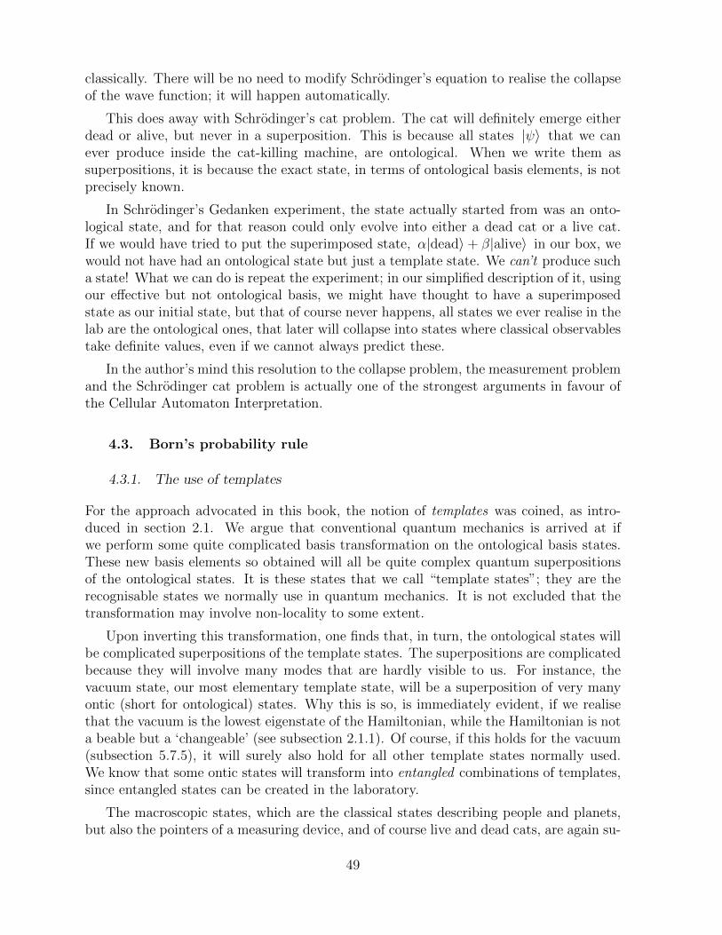
classically. There will be no need to modify Schrodinger’s equation to realise the collapseof the wave function; it will happen automatically.

This does away with Schrodinger’s cat problem. The cat will definitely emerge eitherdead or alive, but never in a superposition. This is because all states |ψ〉 that we canever produce inside the cat-killing machine, are ontological. When we write them assuperpositions, it is because the exact state, in terms of ontological basis elements, is notprecisely known.

In Schrodinger’s Gedanken experiment, the state actually started from was an onto-logical state, and for that reason could only evolve into either a dead cat or a live cat.If we would have tried to put the superimposed state, α|dead〉+ β|alive〉 in our box, wewould not have had an ontological state but just a template state. We can’t produce sucha state! What we can do is repeat the experiment; in our simplified description of it, usingour effective but not ontological basis, we might have thought to have a superimposedstate as our initial state, but that of course never happens, all states we ever realise in thelab are the ontological ones, that later will collapse into states where classical observablestake definite values, even if we cannot always predict these.

In the author’s mind this resolution to the collapse problem, the measurement problemand the Schrodinger cat problem is actually one of the strongest arguments in favour ofthe Cellular Automaton Interpretation.

4.3. Born’s probability rule

4.3.1. The use of templates

For the approach advocated in this book, the notion of templates was coined, as intro-duced in section 2.1. We argue that conventional quantum mechanics is arrived at ifwe perform some quite complicated basis transformation on the ontological basis states.These new basis elements so obtained will all be quite complex quantum superpositionsof the ontological states. It is these states that we call “template states”; they are therecognisable states we normally use in quantum mechanics. It is not excluded that thetransformation may involve non-locality to some extent.

Upon inverting this transformation, one finds that, in turn, the ontological states willbe complicated superpositions of the template states. The superpositions are complicatedbecause they will involve many modes that are hardly visible to us. For instance, thevacuum state, our most elementary template state, will be a superposition of very manyontic (short for ontological) states. Why this is so, is immediately evident, if we realisethat the vacuum is the lowest eigenstate of the Hamiltonian, while the Hamiltonian is nota beable but a ‘changeable’ (see subsection 2.1.1). Of course, if this holds for the vacuum(subsection 5.7.5), it will surely also hold for all other template states normally used.We know that some ontic states will transform into entangled combinations of templates,since entangled states can be created in the laboratory.

The macroscopic states, which are the classical states describing people and planets,but also the pointers of a measuring device, and of course live and dead cats, are again su-

49

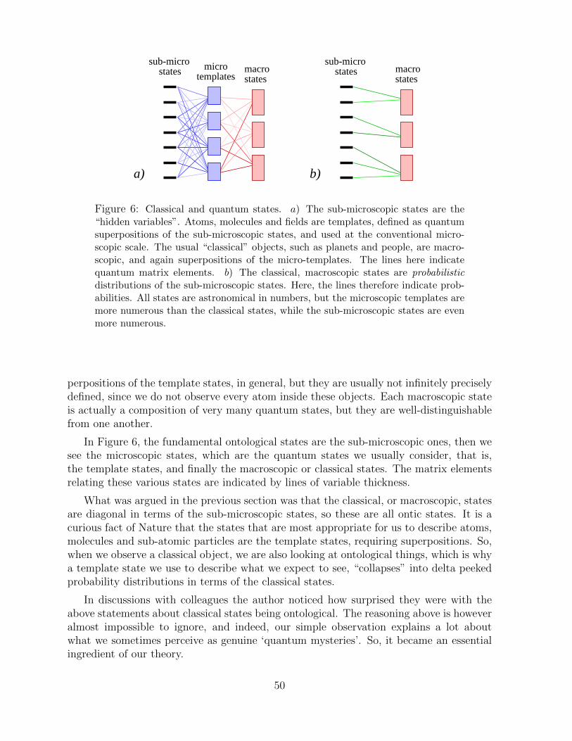
statesmacrostates

sub-micro

statesmacro

templatesmicrostates

sub-micro

b)a)

Figure 6: Classical and quantum states. a) The sub-microscopic states are the“hidden variables”. Atoms, molecules and fields are templates, defined as quantumsuperpositions of the sub-microscopic states, and used at the conventional micro-scopic scale. The usual “classical” objects, such as planets and people, are macro-scopic, and again superpositions of the micro-templates. The lines here indicatequantum matrix elements. b) The classical, macroscopic states are probabilisticdistributions of the sub-microscopic states. Here, the lines therefore indicate prob-abilities. All states are astronomical in numbers, but the microscopic templates aremore numerous than the classical states, while the sub-microscopic states are evenmore numerous.

perpositions of the template states, in general, but they are usually not infinitely preciselydefined, since we do not observe every atom inside these objects. Each macroscopic stateis actually a composition of very many quantum states, but they are well-distinguishablefrom one another.

In Figure 6, the fundamental ontological states are the sub-microscopic ones, then wesee the microscopic states, which are the quantum states we usually consider, that is,the template states, and finally the macroscopic or classical states. The matrix elementsrelating these various states are indicated by lines of variable thickness.

What was argued in the previous section was that the classical, or macroscopic, statesare diagonal in terms of the sub-microscopic states, so these are all ontic states. It is acurious fact of Nature that the states that are most appropriate for us to describe atoms,molecules and sub-atomic particles are the template states, requiring superpositions. So,when we observe a classical object, we are also looking at ontological things, which is whya template state we use to describe what we expect to see, “collapses” into delta peekedprobability distributions in terms of the classical states.

In discussions with colleagues the author noticed how surprised they were with theabove statements about classical states being ontological. The reasoning above is howeveralmost impossible to ignore, and indeed, our simple observation explains a lot aboutwhat we sometimes perceive as genuine ‘quantum mysteries’. So, it became an essentialingredient of our theory.

50

4.3.2. Probabilities

At first sight, it may seem that the notion of probability is lost in our treatment ofquantum mechanics. Our theory is ontic, it describes certainties, not probabilities.

However, probabilities emerge naturally also in many classical systems. Think of howa 19th century scientist would look at probabilities. Two beams of particles cross inan interaction area. How will the particles scatter? Of course, the particles will be toosmall to aim them so precisely that we would know in advance exactly how they meetone another, so we apply the laws of statistics. Without using quantum mechanics, the19th century scientist would certainly know how to compute the angular distribution ofthe scattered particles, assuming some classical interaction potential. The origin of thestatistical nature of the outcome of his calculations is simply traced to the uncertaintyabout the initial state.

In conventional quantum mechanics, the initial state may seem to be precisely known:we have two beams consisting of perfectly planar wave functions; the statistical distri-bution comes about because the wave functions of the final state have a certain shape,and only there, the quantum physicist would begin to compute amplitudes and deducethe scattering probabilities from those. So this looks very different. We are now going toexplain however, that the origin of the statistics in both cases is identical after all.

In our theory, the transition from the classical notation to the quantum notation takesplace when we decide to use a template state |ψ(t)〉 to describe the state of the system.At t = 0 , the coefficients |λA|2 , where (see the remarks following Eq. (2.2))

〈ont(0)A |ψ(0)〉 = λA , (4.3)

determine the probability that we are starting with ontological state #A . We then use ourSchrodinger equation to determine |ψ(t)〉 . When, at some time t1 , the asymptotic out-state is reached, we compute 〈ont(t1)A |ψ(t1)〉 , where now the ontological state representsthe outcome of a particular measurement, say, the particles hitting a detector at somegiven angle. According to quantum mechanics, using the Born rule, the absolute square ofthis amplitude is the probability of this outcome. But, according to our theory, the initialontological states |ont(0)〉A evolved into final ontological states |ont(t1)〉A , so, we haveto use the same coefficients λA . And now, these determine the probability of the givenoutcome. So indeed, we conclude that these probabilities coincide with the probabilitiesthat we started with given ontological in-states.

The final ontological states are the ontological states that lead to a given outcome of theexperiment. Note, that we used superpositions in calculating the transition amplitudes,but the final answers just correspond to the probability that we started with a givenontological in-state that, with certainty, evolved into a given final, classical out-state.

Our template states form a very tiny subset of all ontological states, so that every timewe repeat an experiment, the actual ontic state is a different one. The initial templatestate now does represent the probabilities of the initial ontic states, and because theseare projected into the classical final states, the classical final states obey the Born rule ifthe initial states do. Therefore, we can prove that our theory obeys the Born rule if we

51

know that the initial state does that regarding the ontic modes. If we now postulate thatthe template states used always reflect the relative probabilities of the ontic states of thetheory, then the Born rule appears to be an inevitable consequence. [90]

Most importantly, there is absolutely no reason to attempt to incorporate deviationsfrom Born’s probability interpretation of the Copenhagen interpretation into our theory.Born’s rule will be exactly obeyed; there cannot be systematic, reproducible deviations.Thus, we argue, Born’s rule follows from our requirement that the basis of template statesthat we use is related to the basis of ontological states by an orthonormal, or unitary,transformation.

Thus, we derived that: as long as we use orthonormal transformations to go from onebasis to another, Born’s rule, including the use of absolute squares to represent probabili-ties, is the only correct expression for these probabilities.

5. Concise description of the CA Interpretation

Of course we assume that the reader is familiar with the ‘Schrodinger representation’ aswell as the ‘Heisenberg representation’ of conventional quantum mechanics. We often usethese intermittently.

5.1. Time reversible cellular automata

The Cogwheel Model, which, as described in section 2.2, can be mapped on a Zeemanatom with equally spaced energy levels. It is the prototype of an automaton. All ourdeterministic models can be characterised as ‘automata’. A cellular automaton is anautomaton where the data are imagined to form a discrete, d -dimensional lattice, in ann = d+ 1 dimensional space-time. The elements of the lattice are called ‘cells’, and eachcell can contain a limited amount of information. The data Q(~x, t) in each cell (~x, t)could be represented by an integer, or a set of integers, possibly but not necessarily limitedby a maximal value N . An evolution law prescribes the values of the cells at time t + 1if the values at time t (or t and t − 1 ) are given. Typically, the evolution law for thedata in a cell at the space-time position

(~x, t) , ~x = (x1, x2, · · · , xd) , xi, t ∈ Z , (5.1)

will only depend on the data in neighbouring cells at (~x ′, t − 1) and possibly those at(~x, t− 2) . If, in this evolution law, ‖~x ′− ~x‖ is limited by some bound, then the cellularautomaton is said to obey locality.

Furthermore, the cellular automaton is said to be time-reversible if the data in thepast cells can be recovered from the data at later times, and if the rule for this is alsoa cellular automaton. Time reversibility can easily be guaranteed if the evolution law isassumed to be of the form

Q(~x, t+ 1) = Q(~x, t− 1) + F (~x, Q(t)) , (5.2)

52

where Q(~x, t) represent the data at a given point (~x, t) of the space-time lattice, andF (~x, Q(t)) is some given function of the data of all cells neighbouring the point ~x attime t . The + here stands for addition, addition modulo some integer N , or some othersimple, invertible operation in the space of variables Q . Of course, we then have timereversibility:

Q(~x, t− 1) = Q(~x, t+ 1)− F (~x, Q(t)) , (5.3)

where − is the inverse of the operation + .

The simple cogwheel model allows for both a classical and a quantum mechanicaldescription, without any modification of the physics. We can now do exactly the samething for the cellular automaton. The classical states the automaton can be in, areregarded as an orthonormal set of basis elements of an ontological basis. The evolutionoperator Uop(δt) for one single time step whose duration is δt , is a unitary operator, sothat all its eigen states |Ei〉 are unimodular:

Uop(δt)|Ei〉 = e−iωi |Ei〉 , 0 ≤ ω < 2π , (5.4)

and one can find an operator Hop such that

Uop(δt) = e−iHopδt , 0 ≤ Hop < 2π/δt . (5.5)

However, one is free to add integer multiples of 2π/δt to any of the eigen values ofthis Hamiltonian without changing the expression for Uop , so that there is a lot of free-dom in the definition of Hop . One may add arbitrary phase angles to the eigenstates,|Ei〉 → eiϕi |Ei〉 , and these modifications may also depend on possible conserved quan-tities. Clearly, one can modify the Hamiltonian quite a bit without damaging its use-fulness to generate the evolution operator Uop . In subsection 2.2.2 of section 2.2, it isdemonstrated how quite complex energy spectra can emerge this way in relatively simplegeneralisations of the cogwheel model.

Modifications of this sort in the Hamiltonian may well be needed if we wish to reflectthe locality property of the cellular automaton in the Hamiltonian:

Hop?=∑~x

Hop (~x) , [Hop (~x ′) , Hop (~x) ]→ 0 if ‖~x ′ − ~x‖ 1 , (5.6)

but it is an important mathematical question whether a Hamiltonian obeying Eq. (5.6)can be constructed even if the classical cellular automaton is local in the sense describedabove. This problem is discussed further in subsection 5.6.1, in section 9.1, and in partII, chapters 14 and 22. There, we shall see that the situation can become quite complex.Very good approximations may exist for certain cellular automaton systems with possiblysome modified locality properties and a Hamiltonian that approximately obeys a localityprinciple as in Eq. (5.6).

Note, that a Hamiltonian that obeys (5.6) in combination with Poincare invariancewill correspond to a fully renormalized quantum field theory, with all complexities of that,and this assures that finding a complete mathematical solution to the problems sketchedwill not be easy.

53

5.2. The CAT and the CAI

The Cellular Automaton Theory (CAT) assumes that, once a universal Schrodinger equa-tion has been identified that encapsulates all conceivable phenomena in the universe (aGrand Unified Theory, or a Theory for Everything), it will feature an ontological basisthat maps the system into a classical automaton. It is possible, indeed quite likely, thatthe true automaton of the universe will be more complex than an ‘ordinary’ cellular au-tomaton as sketched here, but it may well share some of its main characteristics. Theextent to which this is so, will have to be sorted out by further research.

How the symmetries of nature will be reflected in these classical rules is also difficultto foresee; it is difficult to imagine how Lorentz invariance and diffeomorphism invariancecan be realised in these classical rules. Probably, they will refer to more general quantumbasis choices. This we will assume, for the time being, see in Part II, chapter 18 onsymmetries.

This theory then does seem to be what is usually called a ‘hidden variable theory’.Indeed, in a sense, our variables are hidden; if symmetry transformations exist that trans-form our basis into another one, which diagonalises different operators, then it will bealmost impossible for us to tell which of these is the ‘true’ ontological basis, and so wewill have different candidates for the ‘hidden variables’, which will be impossible to dis-tinguish in practice.

The Cellular Automaton Interpretation (CAI) [72] takes it for granted that this theoryis correct, even if we will never be able to explicitly identify any ontological basis. Weassume that the templates presently in use in quantum mechanics are to be regarded assuperpositions of ontological states, and that the classical states that describe outcomesof observations and measurements are probabilistic distributions of ontological states. Iftwo classical states are distinguishable, their probabilistic distributions have no ontologicalstate in common (see Fig. 6 b ). The universe is in a single ontological state, never in asuperposition of such states, but, whenever we use our templates (that is, when we performa conventional quantum mechanical calculation), we use superpositions just because theyare mathematically convenient. Note that, because the superpositions are linear, ourtemplates obey the same Schrodinger equation as the ontological states do.

In principle, the transformation from a conventional quantum basis to an ontologicalbasis may be quite complex. Only the eigenvalues of the Hamiltonian will be unaffected,and also in deterministic models, these can form quite general spectra, see Figure 3 c .In group theory language, the Hamiltonians we obtain by transforming to different basischoices, will form one single conjugacy class, characterised by the set of eigenvalues.

Eventually, our quantum system should be directly related to some quantum fieldtheory in the continuum limit. We describe quantum field theories in part II, chapter 20.At first sight, it may seem to be obvious that the Hamiltonian should take the formof Eq. (5.6), but we have to remember that the Hamiltonian definitions (2.8), (2.18),(2.26) and the expressions illustrated in Fig. 3, are only well-defined modulo 2π/δt , sothat, when different, non interacting systems are combined, their Hamiltonians do notnecessarily have to add up.

54

These expressions do show that the Hamiltonian Hop can be chosen in many ways,since one can add any operator that commutes with Hop . Therefore it is reasonable toexpect that a Hamiltonian obeying Eq. (5.6) can be defined. An approach is explained inmuch more detail in Part II, chapter 21, but some ambiguity remains, and convergenceof the procedure, even if we limit ourselves to low energy states, is far from obvious.

What we do see is this: a Hamiltonian obeying Eq. (5.6) is the sum of terms that eachare finite and bounded below as well as above. Such a Hamiltonian must have a groundstate, that is, an eigenstate |∅〉 with lowest eigenvalue, which could be normalised to zero.This eigenstate should be identified with the ‘vacuum’. This vacuum is stationary, even ifthe automaton itself may have no stationary solution. The next-to-lowest eigenstate maybe a one-particle state. In a Heisenberg picture, the fields Q(~x, t) will behave as operatorsQop(~x, t) when we pass on to a basis of template states, and as such they may create one-particle states out of the vacuum. Thus, we arrive at something that resembles a genuinequantum field theory. The states are quantum states in complete accordance with aCopenhagen interpretation. The fields Qop (~x, t) should obey the Wightman axioms.Quantum field theories will further be discussed in chapter 20.

However, if we start from just any cellular automaton, there are three ways in whichthe resulting theory will differ from conventional quantum field theories. One is, of course,that space and time are discrete. Well, maybe there is an interesting ‘continuum limit’,in which the particle mass(es) is(are) considerably smaller than the inverse of the timequantum, but, unless our models are chosen very carefully, this will not be the case.

Secondly, the generic cellular automaton will not even remotely be Lorentz invariant.Not only will the one-particle states fail to exhibit Lorentz invariance, or even Galileiinvariance; the states where particles may be moving with respect to the vacuum statewill be completely different from the static one-particle states. Also, rotation symmetrywill be reduced to some discrete lattice rotation group if anything at all. So, the familiarsymmetries of relativistic quantum field theories will be totally absent.

Thirdly, it is not clear that the cellular automaton can be associated to a singlequantum model or perhaps many inequivalent ones. The addition or removal of otherconserved operators to Hop is akin to the addition of chemical potential terms. In theabsence of Lorentz invariance, it will be difficult to distinguish the different types of‘vacuum’ states one thus obtains.

For all these reasons, most cellular automaton models will be very different from thequantised field theories for elementary particles. The main issue discussed in this book,however, is not whether it is easy to mimic the Standard Model in a cellular automaton,but whether one can obtain quantum mechanics, and something resembling quantumfield theory at least in principle. The origin of the continuous symmetries of the StandardModel will stay beyond what we can handle in this book, but we can discuss the questionto what extent cellular automata can be used to approximate and understand the quantumnature of this world. See our discussion of symmetry features in part II, section 18.

As will be explained later, it may well be that invariance under general coordinatetransformations will be a crucial ingredient in the explanation of continuous symmetries,

55

so it may well be that the ultimate explanation of quantum mechanics will also requirethe complete solution of the quantum gravity problem. We cannot pretend to have solvedthat.

Many of the other models in this book will be explicitly integrable. The cellular au-tomata that we started off with in the first section of this chapter illustrate that ourgeneral philosophy also applies to non-integrable systems. It is generally believed, how-ever, that time reversible cellular automata can be computationally universal [35]. Thismeans that any such automaton can be arranged in special subsets of states that obey therule of any other computationally universal cellular automaton. One would be tempted toargue then, that any computationally universal cellular automaton can be used to mimicsystems as complicated as the Standard Model of the subatomic particles. However, inthat case, being physicists, we would ask for one single special model that is more efficientthan any other, so that any choice of initial state in this automaton describes a physicallyrealisable configuration.

5.3. Motivation

It is not too far-fetched to expect that, one day, quantum gravity will be completelysolved, that is, a concise theory will be phrased that shows an air-tight description of therelevant physical degrees of freedom, and a simple model will be proposed that shows howthese physical variables evolve. We might not even need a conventional time variable forthat, but what we do need is an unambiguous prescription telling us how the physicaldegrees of freedom will look in a region of space-time that lies in the future of a regiondescribed earlier.

A complete theory explaining quantum mechanics can probably not be formulatedwithout also addressing quantum gravity, but what we can do is to formulate our proposal,and to establish the language that will have to be employed. Today, our description ofmolecules, atoms, fields and relativistic subatomic particles is interspersed with wavefunctions and operators. Our operators do not commute with operators describing otheraspects of the same world, and we have learned not to be surprised by this, but justto choose a set of basis elements as we please, guess a reasonable looking Schrodingerequation, and calculate what we should find when we measure things. We were told notto ask what reality is, and this turned out to be a useful advice: we calculate, and weobserve that the calculations make sense. It is unlikely that any other observable aspectsof fields and particles can ever be calculated, it will never be more than what we canderive from quantum mechanics. For example, given a radio-active particle, we cannotcalculate exactly at what moment it will decay. The decay is controlled by a form ofrandomness that we cannot control, and this randomness seems to be far more perfectthan what can be produced using programmed pseudo-random sequences. We are told togive up any hope to outsmart Nature in this respect.

The Cellular Automaton Interpretation (CAI) suggests to us what it is that we actuallydo when we solve a Schrodinger equation. We thought that we are following an infinite setof different worlds, each with some given amplitude, and the final events that we deduce

56

from our calculations depend on what happens in all these worlds. This, according tothe CAI, is an illusion. There is no infinity of different worlds, there is just one, butwe are using the “wrong” basis to describe it. The word “wrong” is here used not tocriticise the founding fathers of quantum mechanics, who made marvellous discoveries,but to repeat what they of course also found out, which is that the basis they are usingis not an ontological one. The terminology used to describe that basis does not discloseto us exactly how our world, our single world, ‘actually’ evolves in time.

Many other proposed interpretations of quantum mechanics exist. These may eitherregard the endless numbers of different worlds all to be real, or they require some sort ofmodification, mutilation rather, to understand how a wave function can collapse to pro-duce measured values of some observable without allowing for mysterious superpositionsat the classical scale.

The CAI proposes to use the complete mathematical machinery that has been de-veloped over the years to address quantum mechanical phenomena. It includes exactlythe Copenhagen prescriptions to translate the calculations into precise predictions whenexperiments are done, so, at this point, definitely no modifications are required.

There is one important way in which we deviate from Copenhagen however. Accordingto Copenhagen, certain questions are not to be asked:

Can it be that our world is just a single world where things happen, accordingto evolution equations that might be fundamentally simpler than Schrodinger’sequation, and are there ways to find out about this? Can one remove theelement of statistical probability distributions from the basic laws of quantummechanics?

According to Copenhagen, there exist no experiments that can answer such questions,and therefore it is silly even to ask them. But what I have attempted to show in thiswork is that not experimentally, but theoretically, we may find answers. We may beable to identify models that describe a single classical world, even if forbiddingly complexcompared to what we are used to, and we may be able to identify its physical degrees offreedom with certain quantum variables that we already know about.

The cellular automaton described in the preceding sections, would be the prototypeexample; it is complicated yet quite possibly not complicated enough. It has symmetries,but in the real world there are much larger symmetry groups, such as the Lorentz orPoincare group, showing relations between different kinds of events, and these are ad-mittedly difficult to implement. The symmetry groups, think of space-time translationsymmetry, may actually be at the roots of the mysterious features that were found in ourquantum world, so that these may have natural explanations.

Why should we want just a single world with classical equations describing its evo-lution? What’s wrong with obeying Copenhagen’s dictum about not asking questions, ifthey will not be experimentally accessible anyway?

According to the author, there will be overwhelming motivations: If a classical modeldoes exist, it will tremendously simplify our view of the world, it will help us once and

57

forever to understand what really happens when a measurement is made and a wavefunction ‘collapses’. It will explain the Schrodinger cat paradox once and for good.

Even more importantly, the quantum systems that allow for a classical interpretationform an extremely tiny subset of all quantum models. If it is indeed true that our worldfalls in that class, which one may consider to be likely after having read all this, then thisrestricts our set of allowable models so much that it may enable us to guess the right one,a guess that otherwise could never have been made. So indeed, what we are really after isa new approach towards guessing what the ‘Theory of the World’ is. We strongly suspectthat, without this superb guide, we will never even come close. Thus, our real motivationis not to be able to better predict the outcomes of experiments, which may not happensoon, but rather to predict which class of models we should scrutinise to find out aboutthe truth.

Let us emphasise once more, that this means that the CAI / CAT will primarily beof importance if we wish to decipher nature’s laws at the most fundamental time- anddistance scales, that is, the Planck scale. Thus, an important new frontier where theempire of the quantum meets the classical world, is proclaimed to be near the Planckiandimensions. As we also brought forward repeatedly, the CAI requires a reformulation ofour standard quantum language also when describing the other important border: thatbetween the quantum empire and the ‘ordinary’ classical world at distance scales largerthan the sizes of atoms and molecules.

The CAI actually has more in common with the original Copenhagen doctrine thanmany other approaches, as will be explained. It will do away with the ‘many worlds’, moreradically than the De Broglie-Bohm interpretation. The CAI assumes the existence of oneor more models of Nature that have not yet been discovered. We do discuss many toymodels. These toy models are not good enough to come anywhere close to the StandardModel, but there is reason to hope that one day such a model will be found. In any case,the CAI will apply only to a tiny sub class of all quantum mechanical models usuallyconsidered to explain the observed world, and for this reason we hope it might be helpfulto pin down the right procedure to arrive at the correct theory.

Other models were exposed in this work, just to display the set of tools that one mightchoose to use.

5.3.1. The wave function of the universe

Standard quantum mechanics can confront us with a question that appears to be difficultto answer: Does the universe as a whole have a wave function? Can we describe that wavefunction? Several responses to this question can be envisaged:

(1) I do not know, and I do not care. Quantum mechanics is a theory about observationsand measurements. You can’t measure the entire universe.

(2) I do care, but I do not know. Such a wave function might be so much entangledthat it will be impossible to describe. Maybe the universe has a density matrix, nota wave function.

58

(3) The universe has no fixed wave function. Every time an observation or measurementis made, the wave function collapses, and this collapse phenomenon does not followany Schrodinger equation.

(4) Yes, the universe has a wave function. It obeys the Schrodinger equation, and atall times the probability that some state |ψ〉 is realised is given by the norm of theinner product squared. Whenever any ‘collapse’ takes place, it always obeys theSchrodinger equation.

The agnostic answers (1) and (2) are scientifically of course defensible. We should limitourselves to observations, so don’t ask silly questions. However, they do seem to admitthat quantum mechanics may not have universal validity. It does not apply to the universeas a whole. Why not? Where exactly is the limit of the validity of quantum mechanics?The ideas expressed in this work were attacked because they allegedly do not agree withobservations, but all observations ever made in atomic and subatomic science appear toconfirm the validity of quantum mechanics, while the answers (1) and (2) suggest thatquantum mechanics should break down at some point. In the CAI, we assume that themathematical rules for the application of quantum mechanics have absolute validity. This,we believe, is not a crazy assumption.

In the same vein, we also exclude answer (3). The collapse should not be regarded as aseparate axiom of quantum mechanics, one that would invalidate the Schrodinger equationwhenever an observation, a measurement, and hence a collapse takes place. Therefore,according to our theory, the only correct answer is answer (4). An apparent problemwith this would be that the collapse would require ‘conspiracy’, a very special choice ofthe initial state because otherwise we might accidentally arrive at wave functions thatare quantum superpositions of different collapsed states. This is where the ontologicalbasis comes to the rescue. If the universe is in an ontological state, its wave function willcollapse automatically, whenever needed. As a result, classical configurations, such as thepositions and velocities of the planets are always described by wave functions that aredelta-peaked at these values of the data, whereas wave functions that are superpositionsof planets in different locations, will never be ontological.

The conclusion of this subsection is that, as long as we work with templates, ouramplitudes are psi-epistemic, as they were in the Copenhagen view, but a psi-ontic wavefunction does exist: the wave function of the universe itself. It is epistemic and ontologicalat the same time.

Now, let us go back to Copenhagen, and formulate the rules. As the reader cansee, in some respects we are even more conservative than the most obnoxious quantumdogmatics.

5.4. The rules

As for the Copenhagen rules that we keep, we emphasise the ones most important to us:

(i) To describe a physical phenomenon, the use of any basis is as legitimate as any other.

59

We are free to perform any transformation we like, and rephrase the Schrodingerequation, or rather, the Hamiltonian employed in it, accordingly. In each basis wemay find a useful description of variables, such as positions of particles, or thevalues of their momenta, or the energy states they are in, or the fields of whichthese particles are the energy quanta. All these descriptions are equally ‘real’ .

But none of the usually employed descriptions are completely real. We often see thatsuperpositions occur, and the phase angles of these superpositions can be measured, oc-casionally. In such cases, the basis used is not an ontological one. In practice, we havelearned that this is just fine; we use all of these different basis choices in order to havetemplates. We shall impose no restrictions on which template is ‘allowed’, or which ofthem may represent the truth ‘better’ than others. Since these are mere templates, realitymay well emerge to be a superposition of different templates.

Curiously, even among the diehards of quantum mechanics, this was often thoughtnot to be self-evident. “Photons are not particles, protons and electrons are”, was whatsome investigators claimed. Photons must be regarded as energy quanta. They certainlythought it was silly to regard the phonon as a particle; it is merely the quantum of sound.Sometimes it is claimed that electric and magnetic fields are the ”true” variables, whilephotons are merely abstract concepts. There were disputes on whether a particle is a trueparticle in the position representation or in the momentum representation, and so on.We do away with all this. All basis choices are equivalent. They are nothing more thana coordinate frame in Hilbert space. As long as the Hamiltonian employed appears tobe such that finite-time evolution operators turn diagonal operators (beables) into non-diagonal ones (superimposables), these basis choices are clearly non-ontological; none ofthem describes what is really happening. As for the energy basis, see subsection 5.6.3.

Note, that this means that it is not really the Hamiltonian that we will be interested in,but rather its conjugacy class. If a Hamiltonian H is transformed into a new Hamiltonianby the transformation

H = GH G−1 , (5.7)

where G is a unitary operator, then the new Hamiltonian H , in the new basis, is justas valid as the previous one. In practice, we shall seek the basis, or its operator G , thatgives the most concise possible expression for H .

(ii) Given a ket state |ψ〉 , the probability for the outcome of a measurement to be de-scribed by a given state |a〉 in Hilbert space, is exactly given by the absolute squareof the inner product 〈a|ψ〉 .

This is the well-known Born rule. We shall never modify its mathematical form; onlythe absolute squares of the inner products can be used. However, there is a limitation inprinciple: the bra state 〈a| must be an ontological state. In practice, this is always thecase: the bras 〈a| usually are represented by the classical observations. The Born rule isoften portrayed as a separate axiom of the Copenhagen Interpretation. In our view it is

60

an inevitable consequence of the mathematical nature of quantum mechanics as a tool toperform calculations, see section 4.3.

The most important point where we depart from Copenhagen is that we make somefundamental assumptions:

(a) We postulate the existence of an ontological basis. It is an orthonormal basis ofHilbert space that is truly superior to the basis choices that we are familiar with. Interms of an ontological basis, the evolution operator for a sufficiently fine mesh oftime variables, does nothing more than permute the states.

How exactly to define the mesh of time variables we do not know at present, and maywell become a subject of debate, particularly in view of the known fact that space-timehas a general coordinate invariance built in. We do not claim to know how to arriveat this construction – it is too difficult. In any case, the system is expected to behaveentirely as a classical construction. Our basic assumption is that a classical evolutionlaw exists, dictating exactly how space-time and all its contents evolve. The evolution isdeterministic in the sense that nothing is left to chance. Probabilities enter only if, dueto our ignorance, we seek our refuge in some non-ontological basis.

(b) When we perform a conventional quantum mechanical calculation, we employ a setof templates for what we thought the wave function is like. These templates, such asthe orthonormal set of solutions of the hydrogen atom, just happen to be the statesfor which we know how they evolve. However, they are in a basis that is a rathercomplicated unitary transformation of the ontological basis.

Humanity discovered that these templates obey Schrodinger equations, and we employthese to compute probabilities for the outcomes of experiments. These equations arecorrect to very high accuracies, but they falsely suggest that there is a ‘multiverse’ ofmany different worlds that interfere with one another. Today, these templates are thebest we have.

(c) Very probably, there are more than one different choices for the ontological basis,linked to one another by Nature’s continuous symmetry transformations such asthe elements of the Poincare group, but possibly also by the local diffeomorphismgroup used in General Relativity. Only one of these ontological bases will be ‘truly’ontological.

Which of them will be truly ontological will be difficult or impossible to determine. Thefact that we shall not be able to distinguish the different possible ontological bases, willpreclude the possibility of using this knowledge to perform predictions beyond the usualquantum mechanical ones. This was not our intention anyway. The motivation for thisinvestigation has alway been that we are searching for new clues for constructing modelsmore refined than the Standard Model.

61

The symmetry transformations that link different (but often equivalent) ontologicalbasis choices are likely to be truly quantum mechanical: operators that are diagonal inone of these ontological bases may be non diagonal in an other. However, in the very endwe shall only use the ‘real’ ontological basis. This will be evident in axiom (e).

(d) Classical states are ontological, which means that classical observables are alwaysdiagonal in the ‘truly’ ontological basis.

This would be more difficult to ‘prove’ from first principles, so we introduce it indeed asan axiom. However, it seems to be very difficult to avoid: it is hard to imagine that twodifferent classical states, whose future evolution will be entirely different in the end, couldhave non-vanishing inner products with the same ontological state.

(e) From the very beginning onwards, the Universe was, and it always will be, in a single,evolving ontological state. This means that not only the observables are diagonal inthe ontological basis, but the wave function always takes the simplest possible form:it is one of the elements of the basis itself, so this wave function only contains asingle 1 and for the rest zeros.

Note that this singles out the ‘true’ ontological basis from other choices, where the physicaldegrees of freedom can also be represented by ‘beables’, that is, operators that at alltimes commute. So, henceforth, we only refer to this one ‘true’ ontological basis as ‘the’ontological basis.

Most importantly, the last two axioms completely solve the measurement problem[25], the collapse question and Schrodinger’s cat paradox. The argument is now simplythat Nature is always in a single ontological state, and therefore it has to evolve into asingle classical state.

5.5. Features of the Cellular Automaton Interpretation (CAI)

A very special feature of the CAI is that ontological states do never form superpositions.From day and time zero onwards, the universe must have been in a single ontological statethat evolves. This is also the reason why it never evolves into a superposition of classicalstates. Now remember that the Schrodinger equation is obeyed by the ontological statesthe universe may be in. This then is the reason why this theory automatically generates‘collapsed wave functions’ that describe the results of a measurement, without ever partingfrom the Schrodinger equation. For the same reason, ontological states can never evolveinto a superposition of a dead cat and a live cat. Regarded from this angle, it actuallyseems hard to see how any other interpretation of quantum mechanics could have survivedin the literature: quantum mechanics by itself would have predicted that if states |ψ 〉 and|χ 〉 can be used as initial states, so can the state α|ψ 〉 + β|χ 〉 . Yet the superpositionof a dead cat and a live cat cannot serve to describe the final state. If |ψ 〉 evolves intoa live cat and |χ 〉 into a dead one, then what does the state α|ψ 〉+ β|χ 〉 evolve into?the usual answers to such questions cannot be correct.19

19I here refer to the argument that decoherence, some way or other, does the job. See section 3.5.

62

The Cellular Automaton Interpretation adds some notions to quantum mechanics thatdo not have any distinguished meaning in the usual Copenhagen view. We introducedthe ontological basis as being, in some sense, superior to any other choice of basis. Onemight naturally argue that this would be a step backwards in physics. Did Copenhagen,in section 5.4, not emphasise that all choices of basis are equivalent? Why would onechoice stand out?

Indeed, what was stated in rule #i in section 5.4 was that all basis choices are equiv-alent, but what we really meant was that all basis choices normally employed are equiv-alent. Once we adopt the Copenhagen doctrine, it does not matter anymore which basiswe choose. Yet there is one issue in the Copenhagen formalism that has been heavily dis-puted in the literature and now is truly recognised as a weakness: the collapse of the wavefunction and the treatment of measurements. At these points the superposition axiomfails. As soon as we admit that one superior basis exists, this weakness disappears. Allwave functions may be used to describe a physical process, but then we have to toleratethe collapse axiom if we do not work in the ontological basis.

The CAI allows us to use a basis that stands out. It stands out because, in thisbasis, we recognise wave functions that are special: the ontological wave functions. In theontological basis, the ontological wave functions are the wave functions that correspondto the basis elements; each of these wave functions contains a one and for the rest zeros.The ontological wave functions exclusively evolve into ontological wave functions again.In this basis, there is no room for chance anymore, and superpositions can be completelyavoided.

The fact that, also in the usual formalism of quantum mechanics, states that start outwith a classical description, such as beams of particles aimed at each other, end up asclassical probability distributions of particles coming out of the interaction region, in ourview can be seen as evidence for an ‘ontology conservation law’, a law that says that anontological basis exists, such that true ontological states at one moment of time, alwaysevolve into true ontological states at later times. This is a new conservation law. It istempting to conclude that the CAI is inevitable.

In the ontological basis, the evolution is deterministic. However, this term must beused with caution. “Deterministic” cannot imply that the outcome of the evolution pro-cess can be foreseen. No human, nor even any other imaginable intelligent being, will beable to compute faster than Nature itself. The reason for this is obvious: our intelligentbeing would also have to employ Nature’s laws, and we have no reason to expect thatNature can duplicate its own actions more efficiently than having them happen in thefirst place. This is how one may restore the concept of “free will”: whatever happens inour brains is unique and unforeseeable by anyone or anything.

5.5.1. Beables, changeables and superimposables

Having a special basis and special wave functions, also allows us to distinguish specialobservables or operators. In standard quantum mechanics, we learned that operators andobservables are indistinguishable, so we use these concepts interchangeably. Now, we will

63

have to learn to restore the distinctions. We repeat what was stated in subsection 2.1.1,operators can be of three different forms:

(I) beables Bop : these denote a property of the ontological states, so that beables arediagonal in the ontological basis |A〉, |B〉, · · · of Hilbert space:

B aop|A〉 = B a(A)|A〉 , (beable) . (5.8)

Beables will always commute with one another, at all times :

[B aop(~x1, t1), B bop(~x2, t2)] = 0 ∀ ~x1, ~x2, t1, t2. (5.9)

Quantised fields, copiously present in all elementary particle theories, do obey Eq. (5.9),but only outside the light cone (where |t1 − t2| < |~x1 − ~x2| ), not inside that cone, whereEqs. (20.29), see Part II, do not hold, as can easily be derived from explicit calculations.Therefore, quantised fields are altogether different from beables.

(II) changeables Cop : operators that replace an ontological state |A〉 by another onto-logical state |B〉 , such as a permutation operator:

Cop|A〉 = |B〉 , (changeable) . (5.10)

Changeables do not commute, but they do have a special relationship with beables; theyinterchange them:

B(1)op Cop = CopB(2)

op . (5.11)

We may want to make an exception for infinitesimal changeables, such as the HamiltonianHop :

[Bop, Hop] = −i ∂∂tBop . (5.12)

(III) superimposables Sop : these map an ontological state onto any other, more generalsuperposition of ontological states:

Sop|A〉 = λ1|A〉+ λ2|B〉+ · · · , (superimposable) . (5.13)

All operators normally used are superimposables, even the simplest position or momentumoperators of classroom quantum mechanics. This is easily verified by checking the time-dependent commutation rules (in the Heisenberg representation). In general20:

[~x(t1), ~x(t2)] 6= 0 , if t1 6= t2 . (5.14)

20A rare exception, for example, is the harmonic oscillator when the time span is an integer multipleof the period T .

64

5.5.2. Observers and the observed

Standard quantum mechanics taught us a number of important lessons. One was thatwe should not imagine that an observation can be made without disturbing the observedobject. This warning is still valid in the CAI. If measuring the position of a particle means

checking the wave function whether perhaps ~x?= ~x(1) , this may be interpreted as having

the operator Pop(~x(1)) act on the state:

|ψ〉 → Pop(~x(1))|ψ〉 , Pop(~x(1)) = δ(~xop − ~x(1)) . (5.15)

This modifies the state, and consequently all operators acting on it after that may yieldresults different from what they did before the “measurement”.

However, when a genuine beable acts on an ontological state, the state is simplymultiplied with the value found, but will evolve in the same way as before (assuming wechose the ‘true’ ontological basis, see axiom # c in section 5.4). Thus, measurements ofbeables are, in a sense, classical measurements.

Other measurements, which seem to be completely legal according to conventionalquantum mechanics, will not be possible in the CAI. In the CAI, as in ordinary quantummechanics, we can consider any operator and study its expectation value. But sincethe class of physically realisable wave functions is now smaller than in standard QM,certain states can no longer be realised, and we cannot tell what the outcome of such ameasurement could possibly be. Think of any (non infinitesimal) changeable Cop . Allontological states will give the ‘expectation value’ zero to such a changeable, but we canconsider its eigenvalues, which in general will not yield the value zero. The correspondingeigenstates are definitely not ontological (see subsection 5.7.1).

Does this mean that standard quantum mechanics is in conflict with the CAI? Weemphasise that this is not the case. It must be realised that, also in conventional quantummechanics, it may be considered acceptable to say that the Universe has been, and willalways be, in one and the same quantum state, evolving in time in accordance with theSchrodinger equation (in the Schrodinger picture), or staying the same (in the Heisenbergpicture). If this state happens to be one of our ontological states then it behaves exactlyas it should. Ordinary quantum mechanics makes use of template states, most of whichare not ontological, but then the real world in the end must be assumed to be in asuperposition of these template states so that the ontological state resurfaces anyway,and our apparent disagreements disappear.

5.5.3. Inner products of template states

In doing technical calculations, we perform transformations and superpositions that leadto large sets of quantum states which we now regard as templates, or candidate modelsfor (sub) atomic processes that can always be superimposed at a later stage to describethe phenomena we observe. Inner products of templates can be studied the usual way.

A template state |ψ〉 can be used to serve as a model of some actually observedphenomenon. It can be any quantum superposition of ontological states |A〉 . The inner

65

product expressions |〈A|ψ〉|2 then represent the probabilities that ontological state |A〉is actually realised.

According to the Copenhagen rule #ii, section 5.4, the probability that the templatestate |ψ1〉 is found to be equal to the state |ψ2〉 , is given by | 〈ψ1|ψ2〉|2 . However,already at the beginning, section 2.1, we stated that the inner product 〈ψ1|ψ2〉 shouldnot be interpreted this way. Even if their inner product vanishes, template states |ψ1〉and |ψ2〉 may both have a non vanishing coefficient with the same ontological state |A〉 .This does not mean that we depart from Copenhagen rule #ii, but that the true wavefunction cannot be just a generic template state; it is always an ontological state |A〉 .This means that the inner product rule is only true if either |ψ1〉 or |ψ2〉 is an ontologicalstate while the other may be a template. We are then considering the probability thatthe template state coincides exactly with one of the ontological states |A〉 . We may usethe Born interpretation of the inner product if the template state in question is used todescribe only a small subspace of all physical degrees of freedom. How the unobserveddegrees of freedom are entangled with this state is then immaterial. Thus, the templatestate then can be assumed to represent a probability distribution of the ontological statesof the universe.

We see that the inner product rule can be used in two ways; one is to describe theprobability distribution of the initial states of a system under consideration, and one isto describe the probability that a given classical state is reached at the end of a quantumprocess. If the Born rule is used to describe the initial probabilities, the same rule can beused to calculate the probabilities for the final states.

5.5.4. Density matrices

Density matrices are used when we neither know exactly the ontological states nor thetemplates. One takes a set of templates |ψi〉 , and attributes to them probabilities Wi ≥ 0 ,such that

∑iWi = 1 . This is called a mixed state. In standard quantum mechanics, one

then finds for the expectation values of an operator O :

〈O 〉 =∑i

Wi 〈ψi|O|ψi〉 = Tr (%O) ; % =∑i

Wi |ψi〉 〈ψi| . (5.16)

The operator % is called the density matrix.

Note that, if the ontologic basis is known, and the operator O is a beable, then theprobabilities are indistinguishable from those generated by a template,

|ψ〉 =∑i

λi|ψonti 〉 , |λi|2 = Wi , (5.17)

since in both cases the density matrix in that basis is diagonal:

% =∑i

Wi |ψonti 〉 〈Ψont

i | . (5.18)

If O is not a beable, the off-diagonal elements of the density matrix may seem to besignificant, but we have to remember that non-beable operators in principle cannot be

66

measured, and this means that the formal distinction between density matrices and tem-plates disappears.

Does this imply that mixed states from now on must be considered to be indistin-guishable from pure template states? Not quite. If several ontological basis choices arepossible, and we do not know the ontic states |ψont〉 , the beable operators are not a prioriknown, and this lack of knowledge will force us to use density matrices with non-diagonalelements in the ontological basis.

Indeed, again, we hit the very core of our present understanding of quantum mechanics.If we do not know what the ontic states are, we have to keep open the option of usingvarious choices of mutually non-commuting operators as our template states, and thenthe density matrix reflects our inability to choose the right ones.

We employ non-commuting sets of operators to characterise a state, before choosingthe operator that will actually be used to measure things. According to the CAI, only thatoperator will represent the beables, the others won’t. This feature was at the center ofour considerations concerning Bell’s inequalities as well as the question posed here aboutthe density matrix.

5.6. The Hamiltonian

As was explained in the Introduction to this chapter, section 5.1, there are many waysto choose a Hamiltonian operator that correctly produces a Schrodinger equation for thetime dependence of a (cellular) automaton. Yet the Hamiltonian for the quantum worldas we know it, and in particular for the Standard Model, is quite unique. How does onederive the ‘correct’ Hamiltonian?

Of course there are conserved quantities in the Standard Model, such as chemical po-tentials, global and local charges, and kinematical quantities such as angular momentum.Those may be added to the Hamiltonian with arbitrary coefficients, but they are usuallyquite distinct from what we tend to call ‘energy’, so it should be possible to dispose ofthem. Then, there are many non-local conserved quantities, which explains the largenumber of possible shifts δEi in Fig. 3, subsection 2.2.2. Most of such ambiguities willbe removed by demanding the Hamiltonian to be local.

5.6.1. Locality

Our starting expressions for the Hamiltonian of a deterministic system are Eqs. (2.8) and(2.26). These, however, converge only very slowly for large values of n . If we apply suchexpansions to the cellular automaton, Eqs. (5.2) and (5.3), we see that the nth term willinvolve interactions over neighbours that are n steps separated. If we write the totalHamiltonian H as

H =∑~x

H(~x) , H(~x) =∞∑n=1

Hn(~x) , (5.19)

67

we see contributions Hn(~x) that involve interactions over n neighbours, with coefficientsdropping typically as 1/n . Typically,

[Hn(~x), Hm(~x ′)] = 0 only if |~x− ~x ′| > n+m , (5.20)

while in relativistic quantum field theories, we have [H(~x), H(~x ′)] = 0 as soon as ~x 6= ~x ′ .Considering that the number of interacting neighbouring cells that fit in a d -dimensionalsphere with radius n , may grow rapidly with n , while the leading terms start out being ofthe order of the Planck energy, we see that this convergence is too slow: large contributionsspread over large distances. This is not the Hamiltonian that has the locality structuretypical for the Standard Model.

Now this should not have been surprising. The eigenvalues of Hamiltonians (2.8) and(2.26) are both bounded to the region (0, 2π/δt) , while any Hamiltonian described byequations such as (5.19), should be extensive: their eigenvalues may grow proportionallyto the volume of space.

A better construction for a cellular automaton is worked out further in part II, chapter21. There, we first introduce the Baker Campbell Hausdorff expansion. In that, also, thelowest terms correspond to a completely local Hamiltonian density, while all terms areextensive. Unfortunately, this also comes at a price that is too expensive for us: the BakerCampbell Hausdorff series does not seem to converge at all in this case. One could arguethat, if used only for states where the total energies are much less than the Planck energy,the series should converge, but we have no proof for that. Our problem is that, in theexpressions used, the intermediate states can easily represent higher energies.

Several attempts were made to arrive at a positive Hamiltonian that is also a spaceintegral over local Hamiltonian densities. The problem is that the cellular automatononly defines a local evolution operator over finite time steps, not a local Hamiltonianthat specifies infinitesimal time evolution. Generically valid formal procedures seem tofail, but if we stick closer to procedures that resemble perturbative quantum field the-ories, we seem to approach interesting descriptions that almost solve the problem. Inchapter 22 of part II, we use second quantisation. This procedure can be summarisedas follows: consider first a cellular automaton that describes various types of particles,all non-interacting. This automaton will be integrable, and its Hamiltonian, H0 , willcertainly obey locality properties, and have a lower bound. Next, one must introduceinteractions as tiny perturbations. This should not be difficult in cellular automata; justintroduce small deviations from the free particle evolution law. These small perturba-tions, even if discrete and deterministic, can be handled perturbatively, assuming thatthe perturbation occurs infrequently, at sufficiently separated spots in space and time.This should lead to something that can reproduce perturbative quantum field theoriessuch as the Standard Model.

Note, that in most quantum field theories, perturbation expansions have been usedwith much success (think for instance of the calculation of the anomalous magnetic mo-ment g − 2 of the electron, which could be calculated and compared with experiment insuperb precision), while it is still suspected that the expansions eventually do not con-verge. The non-convergence, however, sets in at very high orders, way beyond today’s

68

practical limits of accuracy in experiments.

We now believe that this will be the best way to construct a Hamiltonian with prop-erties that can be compared to experimentally established descriptions of particles. But,it is only a strategy; it was not possible to work out the details because the deterministicfree particle theories needed are not yet sufficiently well understood.

Thus, there is still a lot of work to be done in this domain. The questions are technicallyrather involved, and therefore we postpone the details to part II of this book.

5.6.2. The double role of the Hamiltonian

Without a Hamiltonian, theoretical physics would look completely different. In classicalmechanics, we have the central issue that a mechanical system obeys an energy conserva-tion law. The energy is a non negative, additive quantity that is locally well-defined. It isthese properties that guarantee stability of mechanical systems against complete collapseor completely explosive solutions.

The classical Hamiltonian principle is a superb way to implement this mechanism.All that is needed is to postulate an expression for the non-negative, conserved quantitycalled energy, which turns into a Hamiltonian H(~x, ~p ) if we carefully define the dynamicalquantities on which it depends, being canonical pairs of positions xi and momenta pi .The ingenious idea was to take as equation of motion the Hamilton equations

d

dtxi(t) =

∂

∂piH(~x, ~p ) ,

d

dtpi(t) = − ∂

∂xiH(~x, ~p ) . (5.21)

This guarantees that ddtH(~x, ~p ) = 0 . The fact that the equations (5.21) allow for a large

set of mathematical transformations makes the principle even more powerful.

In quantum mechanics, as the reader should know, one can use the same Hamiltonianfunction H to define a Schrodinger equation with the same property: the operator H isconserved in time. If H is bounded from below, this guarantees the existence of a groundstate, usually the vacuum,

Thus, both quantum and classical mechanics are based on this powerful principle,where a single physical variable, the Hamiltonian, does two things: it generates the equa-tions of motion, and it gives a locally conserved energy function that stabilises the solu-tions of the equations of motion. This is how the Hamiltonian principle describes equationsof motion, or evolution equations, whose solutions are guaranteed to be stable.

Now how does this work in discrete, deterministic systems of the kind studied here?Our problem is that, in a discrete, classical system, the energy must also be discrete,but the generator of the evolution must be an operator with continuous eigenvalues. Thecontinuous differential equations (5.21) must be replaced by something else. In principle,this can be done, we could attempt to recover a continuous time variable, and derivehow our system evolves in terms of that time variable. What we really need is andoperator H , that partly represents a positive, conserved energy, and partly a generatorof infinitesimal time changes. We elaborate this issue further in part II, chapter 19, where,

69

among other things, we construct a classical, discretised Hamiltonian in order to apply acellular automaton version of the Hamilton principle.

5.6.3. The energy basis

Beables are operators that commute at all times, and ontological states are eigenstatesof these beables. There is a trivial example of such operators and such states in the realworld: the Hamiltonian and its eigenstates. According to our definition they form a setof beables, but unfortunately, they are trivial: there is only one Hamiltonian, and theenergy eigenstates do not change in time at all. This describes a static classical world.What is wrong with it?

Since we declared that superpositions of ontological states are not ontological, thissolution also tells us that, if the energy eigenstates would be considered as ontological, nosuperpositions of these would be admitted, while all conventional physics only re-emergeswhen we do consider superpositions of the energy eigenstates. Only superpositions ofdifferent energy states can be time-dependent, so yes, this is a solution, but no, it isnot the solution we want. The energy basis solution emerges for instance if we take themodel of section 2.2.2, Figures 2 and 3, where we replace all loops by trivial loops, havingonly a single state, while putting all the physics in the arbitrary numbers δEi . It is inaccordance with the rules, but not useful.

Thus, the choice of the energy basis represents an extreme limit that is often not usefulin practice. We see this also happen when a very important procedure is considered: itseems that we will have to split energy into two parts: on the one hand, there is a large,classical component, where energy, equivalent to mass, acts as the source of a gravitationalfield and as such must be ontological, that is, classical. This part must probably bediscretized. On the other hand, we have the smaller components of the energy that actas eigen values of the evolution operator, over sufficiently large time steps (much largerthan the Planck time). These must form a continuous spectrum.

If we would consider the energy basis as our ontological basis, we regard all of theenergy as classical, but then the part describing evolution disappears; that is not goodphysics. See Part II, Figure 19, in subsection 19.4.1. The closed contours in that figuremust be non-trivial.

5.7. Miscellaneous

5.7.1. The Earth–Mars interchange operator

The CAI surmises that quantum models exist that can be regarded as classical systemsin disguise. If one looks carefully at these classical systems, it seems as if any classicalsystem can be rephrased in quantum language: we simply postulate an element of a basisof Hilbert space to correspond to every classical physical state that is allowed in thesystem. The evolution operator is the permutator that replaces a state by its successorin time, and we may or may not decide later to consider the continuous time limit.

70

Naturally, therefore, we ask the question whether one can reverse the CAI, and con-struct quantum theories for systems that are normally considered classical. The answer isyes. To illustrate this, let us consider the planetary system. It is the prototype of a classi-cal theory. We consider large planets orbiting around a sun, and we ignore non-Newtoniancorrections such as special and general relativity, or indeed the actual quantum effects,all of which being negligible corrections. We regard the planets as point particles, evenif they may feature complicated weather patterns, or life; we just look at their classical,Newtonian equations of motion.

The ontological states are defined by listing the positions ~xi and velocities ~vi of theplanets (which commute), and the observables describing them are the beables. Yet alsothis system allows for the introduction of changeables and superimposables. The quantumHamiltonian here is not the classical thing, but

Hquant =∑i

(~p opx, i · ~vi + ~p op

v, i · ~Fi(x)/mi

), (5.22)

where

~p opx, i = −i ∂

∂~xi, ~p op

v, i = −i ∂∂~vi

, and x = ~xi . (5.23)

Here, ~Fi(x) are the classical forces on the planets, which depend on all positions.Eq. (5.22) can be written more elegantly as

Hquant =∑i

(~p opx, i ·

∂Hclass

∂~pi− ~p op

p, i ·∂Hclass

∂~xi

), (5.24)

where p opp, i = m−1

i p opv, i . Clearly, ~p op

x i , ~p opv i and ~p op

p i are infinitesimal changeables, and sois, of course, the Hamiltonian Hquant . The planets now span a Hilbert space and behaveas if they were quantum objects. We did not modify the physics of the system.

We can continue to define more changeables, and ask how they evolve in time. One ofthe author’s favourites is the Earth–Mars interchange operator. It puts the Earth whereMars is now, and puts Mars where planet Earth is. The velocities are also interchanged21.If Earth and Mars had the same mass then the planets would continue to evolve as ifnothing happened. Since the masses are different however, this operator will have rathercomplicated properties when time evolves. It is not conserved in time.

The eigenvalues of the Earth–Mars interchange operator XEM are easy to calculate:

XEM = ±1 , (5.25)

simply because the square of this operator is one. In standard QM language, XEM is anobservable. It does not commute with the Hamiltonian because of the mass differences,but, at a particular moment, t = t1 , we can consider one of its eigenstates and ask howit evolves.

21We disregarded the moons for a moment; we could drag the moons along as well, or keep them wherethey are. They don’t play a role in this argument.

71

Now why does all this sound so strange? How do we observe XEM ? No-one canphysically interchange planet Earth with Mars. But then, no-one can interchange twoelectrons either, and yet, in quantum mechanics, this is an important operator. Theanswer to these questions is, that regarding the planetary system, we happen to knowwhat the beables are: they are the positions and the velocities of the planets, and thatturns them into ontological observables. The basis in which these observables are diagonaloperators is our preferred basis. The elements of this basis are the ontological states ofthe planets. If, in a quantum world, investigators one day discover what the ontologicalbeables are, everything will be expressed in terms of these, and any other operators areno longer relevant.

It is important to realise that, in spite of the fact that, in Copenhagen language, XEM

is an observable, we cannot measure it, to see whether it is +1 or −1 . This is becausewe know the wave function |ont〉 . It is 1 for the actual positions of Earth and Mars, 0when we interchange the two. This is the superposition

|ont〉 = 1√2

(|XEM = 1 〉+ |XEM = −1 〉

); (5.26)

which is a superposition of two template states. According to Copenhagen, a measurementwould yield ±1 with 50%/50% chances.

5.7.2. Rejecting local counterfactual definiteness and free will

The arguments usually employed to conclude that local hidden variables cannot exist,begin with assuming that such hidden variables should imply local counterfactual defi-niteness. One imagines a set-up such as the EPR-Bell experiment that we exposed insection 3.6. Alice and Bob are assumed to have the ‘free will’ to choose the orientation oftheir polarisation filters anytime and anyway they wish, and there is no need for them toconsult anyone or anything to reach their (arbitrary) decision. The quantum state of thephoton that they are about to investigate should not depend on these choices, nor shouldthe state of a photon depend on the choices made at the other side, or on the outcome ofthose measurements.

This means that the outcomes of measurements should already be determined bysome algorithm long before the actual measurements are made, and also long before thechoice was made what to measure. It is this algorithm that generates conflicts with theexpectations computed in a simple quantum calculation. It is counterfactual, which meansthat there may be one ‘factual’ measurement but there would have been many possiblealternative measurements, measurements that are not actually carried out, but whoseresults should also have been determined. This is what is usually called counterfactualdefiniteness, and it has essentially been disproven by simple logic.

Now, as has been pointed out repeatedly, the violation of counterfactual definitenessis not at all a feature that is limited to quantum theory. In our example of the planetarysystem, subsection 5.7.1, there is no a priori answer to the question which of the twoeigenstates of the Earth-Mars exchange operator, the eigenvalue +1 or −1 , we are in.This is a forbidden, counterfactual question. But in case of the planetary system, we know

72

what the beables are (the positions and velocities of the planets), whereas in the StandardModel we do not know this. There, the illegitimacy of counterfactual statements is notimmediately obvious. In essence, we have to posit that Alice and Bob do not have thefree will to change the orientation of their filters; or if we say that they do, their decisionsmust have their roots in the past and, as such, they affect the possible states a photon canbe in. In short, Alice and Bob make decisions that are correlated with the polarisationsof the photons, as explained in section 3.6.

5.7.3. Entanglement and superdeterminism

An objection often heard against the general philosophy advocated in this work, is that itwould never enable accommodation for entangled particles. The careful reader, however,must realise by now that, in principle, there should be no problem of this sort. Anyquantum state can be considered as a template, and the evolution of these templates willbe governed by the real Schrodinger equation. If the relation between the ontologicalbasis and the more conventional basis choices is sufficiently complex, we will encountersuperimposed states of all sorts, so one definitely also expects states where particles behaveas being ‘quantum-entangled’.

Thus, in principle, it is easy to write down orthonormal transformations that turnontic states into entangled template states.

There are some problems and mysteries, however. The EPR paradox and Bell’s the-orem are examples. As explained in section 3.6, the apparent contradictions can onlybe repaired if we assume rather extensive correlations among the ‘hidden variables’ ev-erywhere in the Universe. The mapping of ontic states into entangled states appears todepend on the settings chosen by Alice and Bob in the distant future.

It seems as if conspiracy takes place: due to some miraculous correlations in theevents at time t = 0 , a pair of photons ‘knows in advance’ what the polarisation anglesof the filters will be that they will encounter later, and how they should pass throughthem. Where and how did this enter in our formalism, and how does a sufficiently naturalsystem, without any conspiracy at the classical level, generate this strange behaviour?

It is not only a feature among entangled particles that may appear to be so problematic.The conceptual difficulty is already manifest at a much more basic level. Consider a singlephoton, regardless whether it is entangled with other particles or not. Our description ofthis photon in terms of the beables dictates that these beables behave classically. Whathappens later, at the polarisation filter(s), is also dictated by classical laws. These classicallaws in fact dictate how myriads of variables fluctuate at what we call the Planck scale, ormore precisely, the smallest scale where distinguishable physical degrees of freedom can berecognised, which may or may not be close to what is usually called the Planck scale. Sinceentangled particles occur in real experiments, we claim that the basis-transformationswill be sufficiently complex to transform states that are ontic at the Planck scale, intoentangled states.

But this is not the answer to the question posed. The usual way to phrase the questionis to ask how ‘information’ is passed on. Is this information classical or quantum? If it

73

is true that the templates are fundamentally quantum templates, we are tempted to say,well, the information passed on is quantum information. Yet it does reduce to classicalinformation at the Planck scale, and this was generally thought not to be possible.

That must be a mistake. As we saw in section 3.6, the fundamental technical contra-diction goes away if we assume strong correlations between the quantum fluctuations –including the vacuum fluctuations – at all distance scales (also including correlations be-tween the fluctuations generated in quasars that are separated by billions of light years).We think the point is the following. When we use templates, we do not know in advancewhich basis one should pick to make them look like the ontological degrees of freedom aswell as possible. For a photon going through a polarisation filter, the basis closest to theontological one is the basis where coordinates are chosen to be aligned with the filter. Butthis photon may have been emitted by a quasar billions of years ago, how did the quasarknow what the ontological basis is?

The answer is that indeed the quasar knows what the ontological basis is, because ourtheory extends to these quasars as well. The information, ‘this is an ontological state,and any set of superimposed states is not’, is a piece of information that, according to ourtheory, is absolutely conserved in time. So, if that turns out to be the basis now, it wasthe basis a billion years ago. The quasars seem to conspire in a plot to make fools of ourexperimenters, but in reality they just observe a conservation law: the information as towhich quantum states form the ontological basis, is conserved in time. Much like the lawof angular momentum, or any other exactly conserved entity, this conservation law tellsus what this variable is in the future if it is known in the past, and vice-versa.

We must conclude that, if there seems to be conspiracy in our quantum description ofreality, then that is to be considered as a feature of our quantum techniques, not of thephysical system we are looking at. There is no conspiracy in the classical description ofthe cellular automaton. Apparent conspiracy is a feature, not a bug.

The answer given here, is often called superdeterminism. It is the idea that indeed Aliceand Bob can only choose ontological states to be measured, never the superimposed states,which we use as templates. In a sense, their actions were predetermined, but of coursein a totally unobservable way. Superdeterminism only looks weird if one adheres to thedescription of entangled particles as being quantum systems, described by their quantumstates. The ontological description does not use quantum states. In that description,the particles behave in a normal, causal manner. However, we do have to keep in mindthat these particles, and everything else, including Bob and Alice’s minds, are all stronglycorrelated. They are correlated now as strongly as when the photons were emitted by thesource, as was laid down22 in the mouse-dropping function, Fig. 5 in subsection 3.6.1.

In subsection 10.3.4, it is explained in explicitly physical terms, what ‘free will’ shouldreally stand for, and why superdeterminism can clash with it.

22The mouse-dropping function does not show a 100% correlation. This is a feature due to the somewhatartificial nature of the model used for the detection. If we use more realistic models for the detection,the mouse-dropping function might consist of sharper peaks.

74

5.7.4. The superposition principle in Quantum Mechanics

What exactly happened to the superposition principle in the CA Interpretation of quan-tum mechanics? Critics of our work brought forward that the CAI disallows superposition,while obviously the superposition principle is serving quite well as a solid back bone ofquantum mechanics. Numerous experiments confirm that if we have two different states,also any superposition of these states can be realised. Although the reader should haveunderstood by now how to answer this question, let us attempt to clarify the situationonce again.

At the most basic level of physical law, we assume only ontological states to occur,and any superposition of these, in principle, does not correspond to an ontological state.At best, a superposition can be used to describe probabilistic distributions of states (wecall these “template states”, to be used when we do not have the exact information athand to determine with absolute certainty which ontological state we are looking at). Inour description of the Standard Model, or any other known physical system such as atomsand molecules, we do not use ontological states but templates, which can be regarded assuperpositions of ontological states. The hydrogen atom is a template, all elementaryparticles we know about are templates, and this means that the wave function of theuniverse, which is an ontological state, must be a superposition of our templates. Whichsuperposition? Well, we will encounter many different superpositions when doing repeatedexperiments. This explains why we were led to believe that all superpositions are alwaysallowed.

But not literally all superpositions can occur. Superpositions are man-made. Ourtemplates are superpositions, but that is because they represent only the very tiny sectorof Hilbert space that we understand today. The entire universe is in only one ontologicalstate at the time, and it of course cannot go into superpositions of itself. This factnow becomes manifestly evident when we consider the “classical limit”. In the classicallimit we again deal with certainties. Classical states are also ontological. When we do ameasurement, by comparing the calculated “template state” with the ontological classicalstates that we expect in the end, we recover the probabilities by taking the norm squaredof the amplitudes. Classical states also never go into superpositions of classical states.Such superpositions never occur.

It appears that for many scientists this is difficult to accept. During a whole century wehave been brainwashed with the notion that superpositions occur everywhere in quantummechanics. At the same time we were told that if you try to superimpose classical states,you will get probabilistic distributions instead. It is here that our present theory is moreaccurate: if we knew the wave function of the universe exactly, we would find that it alwaysevolves into one classical state only, without uncertainties and without superpositions.

Of course this does not mean that standard quantum mechanics would be wrong. Ourknowledge of the template states, and how these evolve, is very accurate today. It is onlybecause it is not yet known how to relate these template states to the ontological states,that we have to perform superpositions all the time when we do quantum mechanicalcalculations. They do lead to statistical distributions in our final predictions, rather than

75

certainties. This could only change if we would find the ontological states, but since eventhe vacuum state is expected to be a template, and as such a complicated superpositionof uncountably many ontic states, we should expect quantum mechanics to stay with usforever – but as a mathematical tool, not as a mystic departure from classical logic.

5.7.5. The vacuum state

Is the vacuum state an ontological state? The vacuum state is generally defined to be thestate with lowest energy. This also means that no particles can be found in this state,simply because particles represent energy, and, in the vacuum state, we have not enoughenergy even to allow for the presence of a single particle.

The discretised Hamiltonian is only introduced in section 19 of part II. It is a beable,but being discrete it can only be a rough approximation of the quantum Hamiltonian atbest, and its lowest energy state is highly degenerate. As such, this is not good enoughto serve as a definition of a vacuum. More to the point, the Hamiltonian defined insection 19.2 is quantised in units that seem to be as large as the Planck mass. It willbe clear that the Hamiltonian to be used in any realistic Schrodinger equation has amuch more dense, basically continuous, eigenvalue spectrum. The quantum Hamiltonianis definitely not a beable, as we explained earlier above, in section 5.6.3. Therefore, thevacuum is not an ontological state.

In fact, according to quantum field theories, the vacuum contains many virtual par-ticles or particle-antiparticle pairs that fluctuate in- and out of existence everywhere inspace-time. This is typical for quantum superpositions of ontological states. Furthermore,the lightest particles in our theories are much lighter than the Planck mass. They are notontological, and demanding them to be absent in our vacuum state inevitably turns ourvacuum itself also into a non-ontological state.

This is remarkable, because our vacuum state has one more peculiar property: itsenergy density itself is almost perfectly vanishing. Due to the cosmological constant,there is energy in our vacuum state, but it is as small as about 6 protons per m3 , anextremely tiny number indeed, considering the fact that most length scales in particlephysics are indeed much smaller than a metre. This very tiny but non-vanishing numberis one of Nature’s greater mysteries.

And yet, the vacuum appears to be non-ontological, so that it must be a place fullof activity. How to reconcile all these apparently conflicting features is not completelyunderstood.

The vacuum fluctuations may be seen as one of the primary causes of non-vanishing,non-local correlations, such as the mouse dropping function of section 3.6. Without thevacuum fluctuations, it would be difficult to understand how these correlations could besustained.

76

5.7.6. Exponential decay

Vacuum fluctuations must be the primary reason why isolated systems such as atomsand molecules in empty space, show typical quantum features. A very special quantummechanical property of many particles is the way they can decay into two or more otherparticles. Nearly always, this decay follows a perfect exponential decay law: the probabil-ity P (t) that the particle of a given type has not yet decayed after elapsed time t obeysthe rule

dP (t)

dt= −λP (t) , → P (t) = P (0)e−λt , (5.27)

where λ is a coefficient that often does not at all depend on external circumstances, or ontime. If we start off with N0 particles, then the expectation value 〈N(t)〉 of the particlenumber N(t) after time t follows the same law:

〈N(t)〉 = N0 e−λt . (5.28)

If there are various modes in which the particle can decay, we have λ = λ1 +λ2 + . . . ,and the ratios of the λi equals the ratios of the modes of the decays observed.

Now how can this be explained in a deterministic theory such as a cellular automaton?In general, this would not be possible if the vacuum would be a single ontological state.Consider particles of a given type. Each individual particle will decay after a differentamount of time, precisely in accordance to Eq. (5.27). Also, the directions in which thedecay products will fly will be different for every individual particle, while, if there arethree or more decay products involved, also the energy of the various decay products willfollow a probability distribution. For many existing particles, these distributions can beaccurately calculated following the quantum mechanical prescriptions.

In a deterministic theory, all these different decay modes would have to correspondto distinct initial states. This would be hopeless to accommodate for if every individualparticle would have to behave like a ‘glider solution’ of a cellular automaton, since allthese different decay features would have to be represented by different gliders. Onewould quickly find that millions, or billions of different glider modes would have to exist.

The only explanation of this feature must be that the particles are surrounded by avacuum that is in a different ontological state every time. A radio-active particle is con-tinuously hit by fluctuating features in its surrounding vacuum. These features representinformation that flies around, and as such, must be represented by almost perfect randomnumber generators. The decay law (5.27) thus emerges naturally.

Thus it is inevitable that the vacuum state has to be regarded as a single template state,which however is composed of infinitely many ontological states. The states consisting ofa single particle roaming in a vacuum form a simple set of different template states, allorthogonal to the vacuum template state, as dictated in the Fock space description ofparticle states in quantum field theory.

77

5.7.7. A single photon passing through a sequence of polarisers

It is always illustrative to reduce a difficulty to its most basic form. The conceptualdifficulty one perceives in Bell’s gedanken experiment, already shows up if we consider asingle photon, passing through a sequence of polarisation filters, F1, . . . , FN . Imaginethese filters to be rotated by angles ϕ1, ϕ2, . . . , ϕN , and every time a photon hits oneof these filters, say Fn , there is a probability equal to sin2 ψn , with ψn = ϕn−1 − ϕn ,that the photon is absorbed by this filter. Thus, the photon may be absorbed by any ofthe N polarisers. What would an ontological description of such a setup be like?

Note that, the setup described here resembles our description of a radio-active par-ticle, see the previous subsection. There, we suggested that the particle is continuouslyinteracting with the surrounding vacuum. Here, it is easiest to assume that the photoninteracts with all filters. The fact that the photon arrives at filter Fn as a superpositionof two states, one that will pass through and one that will be absorbed, means that,in the language of the ontological theory, we have an initial state that we do not quiteknow; there is a probability cos2 ψn that we have a photon of the pass-through type, anda probability sin2 ψn that it is of the type that will be absorbed. If the photon passesthrough, its polarisation is again well-defined to be ϕn . This will determine what thedistribution is of the possible states that may or may not pass through the next filter.

We conclude that the filter, being essentially classical, can be in a very large numberof distinct ontological states. The simplest of all ontological theories would have it thata photon arrives with polarisation angle ψn with respect to the filter. Depending onthe ontological state of the filter, we have probability cos2 ψ that the photon is allowedthrough, but rotated to the direction ϕn , and probability sin2 ψ that it is absorbed (orreflected and rotated).

Now, return to the two entangled photons observed by Alice and Bob in Bell’s set-up. In the simplest of all ontological theories, this is what happens: Alice’s and Bob’sfilters act exactly as above. The two photons carry both the same information in theform of a single angle, c . Alice’s filter has angle a , Bob’s has angle b . As we sawin subsection 3.6.1, there is a 3-point correlation between a , b and c , given by themouse-dropping function, (3.26) and Fig. 5.

Now note, that the mouse-dropping function is invariant under rotations of a , band/or c by 90 . The nature of the ontological state depends very precisely on theangles a , b , and c , but each of these states differs from the others by multiples of 90

in these angles. Therefore, as soon as we have picked the desired orthonormal basis, thebasis elements will be entirely uncorrelated. This makes the correlations unobservablewhenever we work with the templates. Assuming the ontological conservation law atwork here, we find that the ontological nature of the angles a , b and c is correlated,but not the physical observables. It is to be expected that correlations of this sort willpervade all of physics.

78

5.8. The quantum computer

Quantum mechanics is often endowed with mysterious features. There are vigorous at-tempts to turn some of these features to our advantage. One famous example is thequantum computer. The idea is to use entangled states of information carriers, whichcould be photons, electrons, or something else, to represent vastly more information thanordinary bits and bytes, and are therefore called qubits.

Since the machines that investigators plan to construct would obey ordinary quantummechanics, they should behave completely in accordance with our theories and models.However, this seems to lead to contradictions.

In contrast with ordinary computers, the amount of information that can be carriedby qubits in a quantum computer, in principle, increases exponentially with the numberof cells, and consequently, it is expected that quantum computers will be able to performcalculations that are fundamentally impossible in ordinary computers. An ordinary, clas-sical computer would never be able to beat a quantum computer even if it took the sizeof the universe, in principle.

Our problem is then, that our models underlying quantum mechanics are classical,and therefore they can be mimicked by classical computers, even if an experimentalistwould build a ‘quantum computer’ in such a world. Something is wrong.

Quantum computers still have not been constructed however. There appear to benumerous practical difficulties. One difficulty is the almost inevitable phenomenon ofdecoherence. For a quantum computer to function impeccably, one needs to have perfectqubits.

It is generally agreed that one cannot make perfect qubits, but what can be done iscorrect them for the errors that may sometimes occur. In a regular computer, errors caneasily be corrected, by using a slight surplus of information to check for faulty memorysites. Can the errors of qubits also be corrected? There are claims that this can be done,but in spite of that, we still don’t have a functioning quantum computer, let alone aquantum computer that can beat all classical computers. Our theory comes with a firmprediction:

Yes, by making good use of quantum features, it will be possible in principle,to build a computer vastly superior to conventional computers, but no, thesewill not be able to function better than a classical computer would do, if itsmemory sites would be scaled down to one per Planckian volume element (or,in view of the holographic principle, one memory site per Planckian surfaceelement), and if its processing speed would increase accordingly, typically oneoperation per Planckian time unit of 10−43 seconds.

Such scaled classical computers can of course not be built, so that this quantum computerwill still be allowed to perform computational miracles, but factoring a number withmillions of digits into its prime factors will not be possible – unless fundamentally improvedclassical algorithms turn out to exist. If engineers ever succeed in making such quantum

79

computers, it seems to me that the CAT is falsified; no classical theory can explainquantum mechanics.

6. Quantum gravity

The Planck scale has been mentioned many times already. It is the scale of time, lengths,masses, and energies, where three grand physical theories all play equally significant roles,being special relativity (where the speed of light c is essential), quantum mechanics (withPlanck’s constant ~ ) and Newton’s theory of gravity (with Newton’s constant G ). Having

c = 299 792 458 m/s ,

~ = 1.05457× 10−34 kgm2/s ,

G = 6.674× 10−11 m3kg−1s−2 , (6.1)

one findsthe Planck length, LPl =

√G ~c3

= 1.616× 10−35 m , (6.2)

the Planck time, TPl =√

G ~c5

= 5.391× 10−44 s , (6.3)

the Planck mass, MPl =√

c ~G

= 21.76 µg , (6.4)

and the Planck energy, EPl =√

c5 ~G

= 1.956× 109 J . (6.5)

In this domain of physics, one expects Special and General Relativity and QuantumMechanics all to be relevant, but a complete synthesis of these three has not yet beenachieved – in fact, our continued struggle towards finding such a synthesis was one of themain motivations for this work.

It is not unreasonable to suspect that the Planck length is the smallest significantlength scale in physics, and the Planck time is the smallest time scale at which thingscan happen, but there is more. General Relativity is known to cause space and time tobe curved, so, if one might talk of some “lattice” in space and time, curvature may beexpected to cause defects in this lattice. Alternatively, one might suspect that lattice-likebehaviour can also be realised by imposing a cutoff in local momentum and energy scales(a so-called bandwidth cut-off [50]); however, with such a cut-off deterministic models aredifficult to construct.

It is also important to note that General Relativity is based on the local automorphismgroup. This means that time translations are locally defined, so that one may expect thatgravity could be essential to realise locality requirements for the Hamiltonian. Mass,energy and momentum are local sources of gravitational fields, but there is more.

Gravitation is a destabilising force. Causing masses to attract one another, it gen-erates greater masses and thus even stronger attraction. This may lead to gravitationalimplosion. In contrast, electric as well as magnetic charges act repulsively (if they haveequal signs), which makes electromagnetism a lot more stable than gravity as a forcesystem.

80

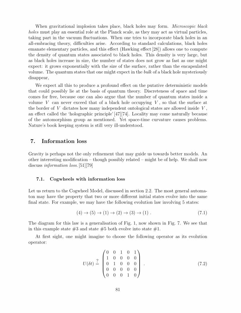
When gravitational implosion takes place, black holes may form. Microscopic blackholes must play an essential role at the Planck scale, as they may act as virtual particles,taking part in the vacuum fluctuations. When one tries to incorporate black holes in anall-embracing theory, difficulties arise. According to standard calculations, black holesemanate elementary particles, and this effect (Hawking effect [28]) allows one to computethe density of quantum states associated to black holes. This density is very large, butas black holes increase in size, the number of states does not grow as fast as one mightexpect: it grows exponentially with the size of the surface, rather than the encapsulatedvolume. The quantum states that one might expect in the bulk of a black hole mysteriouslydisappear,

We expect all this to produce a profound effect on the putative deterministic modelsthat could possibly lie at the basis of quantum theory. Discreteness of space and timecomes for free, because one can also argue that the number of quantum states inside avolume V can never exceed that of a black hole occupying V , so that the surface atthe border of V dictates how many independent ontological states are allowed inside V ,an effect called the ‘holographic principle’ [47][74]. Locality may come naturally becauseof the automorphism group as mentioned. Yet space-time curvature causes problems.Nature’s book keeping system is still very ill-understood.

7. Information loss

Gravity is perhaps not the only refinement that may guide us towards better models. Another interesting modification – though possibly related – might be of help. We shall nowdiscuss information loss. [51][79]

7.1. Cogwheels with information loss

Let us return to the Cogwheel Model, discussed in section 2.2. The most general automa-ton may have the property that two or more different initial states evolve into the samefinal state. For example, we may have the following evolution law involving 5 states:

(4)→ (5)→ (1)→ (2)→ (3)→ (1) . (7.1)

The diagram for this law is a generalisation of Fig. 1, now shown in Fig. 7. We see thatin this example state #3 and state #5 both evolve into state #1.

At first sight, one might imagine to choose the following operator as its evolutionoperator:

U(δt)?=

0 0 1 0 11 0 0 0 00 1 0 0 00 0 0 0 00 0 0 1 0

. (7.2)

81

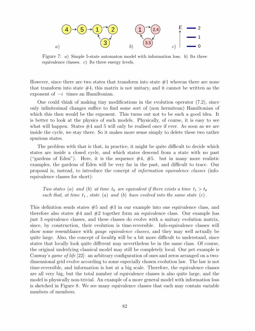
a)

54

3

21

b)

1

3,5

2,4

c)

2

1

0

E

Figure 7: a) Simple 5-state automaton model with information loss. b) Its threeequivalence classes. c) Its three energy levels.

However, since there are two states that transform into state #1 whereas there are nonethat transform into state #4, this matrix is not unitary, and it cannot be written as theexponent of −i times an Hamiltonian.

One could think of making tiny modifications in the evolution operator (7.2), sinceonly infinitesimal changes suffice to find some sort of (non hermitean) Hamiltonian ofwhich this then would be the exponent. This turns out not to be such a good idea. Itis better to look at the physics of such models. Physically, of course, it is easy to seewhat will happen. States #4 and 5 will only be realised once if ever. As soon as we areinside the cycle, we stay there. So it makes more sense simply to delete these two ratherspurious states.

The problem with that is that, in practice, it might be quite difficult to decide whichstates are inside a closed cycle, and which states descend from a state with no past(“gardens of Eden”). Here, it is the sequence #4, #5. but in many more realisticexamples, the gardens of Eden will be very far in the past, and difficult to trace. Ourproposal is, instead, to introduce the concept of information equivalence classes (info-equivalence classes for short):

Two states (a) and (b) at time t0 are equivalent if there exists a time t1 > t0such that, at time t1 , state (a) and (b) have evolved into the same state (c) .

This definition sends states #5 and #3 in our example into one equivalence class, andtherefore also states #4 and #2 together form an equivalence class. Our example hasjust 3 equivalence classes, and these classes do evolve with a unitary evolution matrix,since, by construction, their evolution is time-reversible. Info-equivalence classes willshow some resemblance with gauge equivalence classes, and they may well actually bequite large. Also, the concept of locality will be a bit more difficult to understand, sincestates that locally look quite different may nevertheless be in the same class. Of course,the original underlying classical model may still be completely local. Our pet example isConway’s game of life [22]: an arbitrary configuration of ones and zeros arranged on a two-dimensional grid evolve according to some especially chosen evolution law. The law is nottime-reversible, and information is lost at a big scale. Therefore, the equivalence classesare all very big, but the total number of equivalence classes is also quite large, and themodel is physically non-trivial. An example of a more general model with information lossis sketched in Figure 8. We see many equivalence classes that each may contain variablenumbers of members.

82

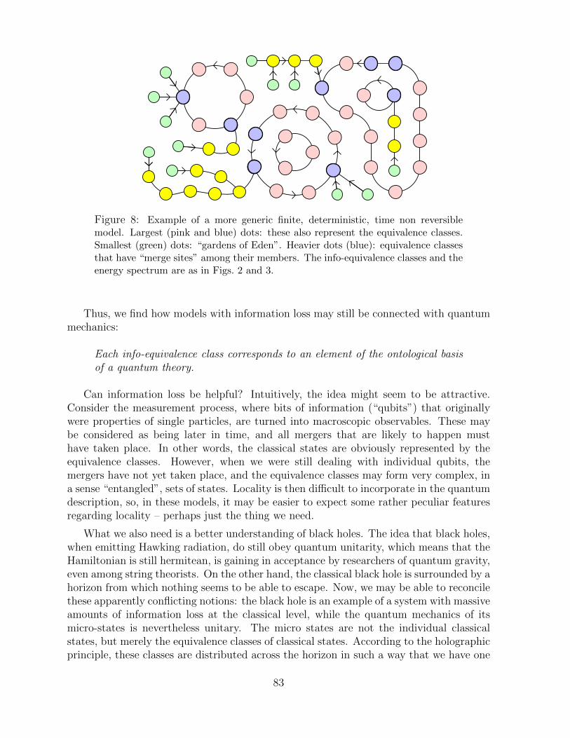
Figure 8: Example of a more generic finite, deterministic, time non reversiblemodel. Largest (pink and blue) dots: these also represent the equivalence classes.Smallest (green) dots: “gardens of Eden”. Heavier dots (blue): equivalence classesthat have “merge sites” among their members. The info-equivalence classes and theenergy spectrum are as in Figs. 2 and 3.

Thus, we find how models with information loss may still be connected with quantummechanics:

Each info-equivalence class corresponds to an element of the ontological basisof a quantum theory.

Can information loss be helpful? Intuitively, the idea might seem to be attractive.Consider the measurement process, where bits of information (“qubits”) that originallywere properties of single particles, are turned into macroscopic observables. These maybe considered as being later in time, and all mergers that are likely to happen musthave taken place. In other words, the classical states are obviously represented by theequivalence classes. However, when we were still dealing with individual qubits, themergers have not yet taken place, and the equivalence classes may form very complex, ina sense “entangled”, sets of states. Locality is then difficult to incorporate in the quantumdescription, so, in these models, it may be easier to expect some rather peculiar featuresregarding locality – perhaps just the thing we need.

What we also need is a better understanding of black holes. The idea that black holes,when emitting Hawking radiation, do still obey quantum unitarity, which means that theHamiltonian is still hermitean, is gaining in acceptance by researchers of quantum gravity,even among string theorists. On the other hand, the classical black hole is surrounded by ahorizon from which nothing seems to be able to escape. Now, we may be able to reconcilethese apparently conflicting notions: the black hole is an example of a system with massiveamounts of information loss at the classical level, while the quantum mechanics of itsmicro-states is nevertheless unitary. The micro states are not the individual classicalstates, but merely the equivalence classes of classical states. According to the holographicprinciple, these classes are distributed across the horizon in such a way that we have one

83

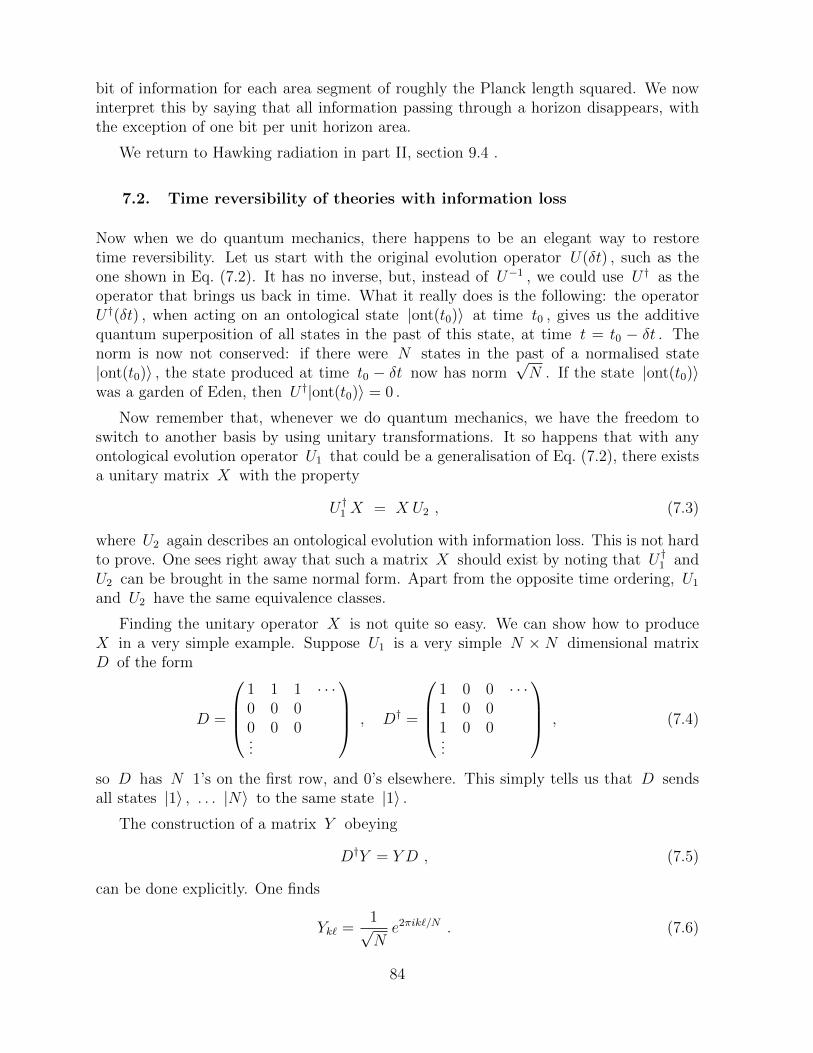
bit of information for each area segment of roughly the Planck length squared. We nowinterpret this by saying that all information passing through a horizon disappears, withthe exception of one bit per unit horizon area.

We return to Hawking radiation in part II, section 9.4 .

7.2. Time reversibility of theories with information loss

Now when we do quantum mechanics, there happens to be an elegant way to restoretime reversibility. Let us start with the original evolution operator U(δt) , such as theone shown in Eq. (7.2). It has no inverse, but, instead of U−1 , we could use U † as theoperator that brings us back in time. What it really does is the following: the operatorU †(δt) , when acting on an ontological state |ont(t0)〉 at time t0 , gives us the additivequantum superposition of all states in the past of this state, at time t = t0 − δt . Thenorm is now not conserved: if there were N states in the past of a normalised state|ont(t0)〉 , the state produced at time t0 − δt now has norm

√N . If the state |ont(t0)〉

was a garden of Eden, then U †|ont(t0)〉 = 0 .

Now remember that, whenever we do quantum mechanics, we have the freedom toswitch to another basis by using unitary transformations. It so happens that with anyontological evolution operator U1 that could be a generalisation of Eq. (7.2), there existsa unitary matrix X with the property

U †1 X = X U2 , (7.3)

where U2 again describes an ontological evolution with information loss. This is not hardto prove. One sees right away that such a matrix X should exist by noting that U †1 andU2 can be brought in the same normal form. Apart from the opposite time ordering, U1

and U2 have the same equivalence classes.

Finding the unitary operator X is not quite so easy. We can show how to produceX in a very simple example. Suppose U1 is a very simple N × N dimensional matrixD of the form

D =

1 1 1 · · ·0 0 00 0 0...

, D† =

1 0 0 · · ·1 0 01 0 0...

, (7.4)

so D has N 1’s on the first row, and 0’s elsewhere. This simply tells us that D sendsall states |1〉 , . . . |N〉 to the same state |1〉 .

The construction of a matrix Y obeying

D†Y = Y D , (7.5)

can be done explicitly. One finds

Yk` =1√Ne2πik`/N . (7.6)

84

Y is unitary and it satisfies Eq. (7.5), by inspection.

This result may come unexpected. Intuitively, one might think that information losswill make our models non-invariant under time reversal. Yet our quantum mechanicaltool does allow us to invert such a model in time. A “quantum observer” in a modelwith information loss may well establish a perfect validity of symmetries such as CPTinvariance. This is because, for a quantum observer, transformations with matrices Xmerely represent a transition to another orthonormal basis; the matrix Y is basically thediscrete Fourier transform matrix. Note that merger states (see Fig. 8) transform intoGardens of Eden, and vice versa.

7.3. The arrow of time

One of the surprising things that came out of this research is a new view on the arrowof time. It has been a long standing mystery that the local laws of physics appear to beperfectly time-reversible, while large-scale, classical physics is not at all time-reversible.Is this not a clash with the reduction principle? If large-scale physics can be deducedfrom small-scale physics, then how do we deduce the fact that the second law of thermo-dynamics dictates that entropy of a closed system can only increase and never decrease?

Most physicists are not really worried by this curious fact. In the past, this authoralways explained the ‘arrow of time’ by observing that, although the small-scale laws ofnature are time-reversible, the boundary conditions are not: the state of the universe wasdictated at time t = 0 , the Big Bang. The entropy of the initial state was very small,probably just zero. There cannot be any boundary condition at the Big Apocalypse,t = t∞ . So, there is asymmetry in time and that is that. For some reason, someresearchers are not content with such a simple answer.

We now have a more radical idea: the microscopic laws may not at all be time-reversible. The classical theory underlying quantum mechanics does not have to be, seesubsection 7.1. Then, in subsection 7.2, we showed that, even if the classical equationsfeature information loss at a great scale – so that only tiny fractions of information arepreserved – the emerging quantum mechanical laws continue to be exactly time-reversible,so that, as long as we adhere to a description of things in terms of Hilbert space, we cannotunderstand the source of time asymmetry.

However, the classical, ontological states are very asymmetric in time, because, as westated, these are directly linked to the underlying classical degrees of freedom.

All this might make information loss acceptable in theories underlying quantum the-ory. Note, furthermore, that our distinction of the ontological states should be kept,because classical states are ontological. Ontological states no not transform into onto-logical states under time reversal, since the transformation operators X and Y involvequantum superpositions. In contrast, templates are transformed into templates. Thismeans automatically that classical states (see section 4.2), are not invariant under timereversal. Indeed, they do not look invariant under time reversal, since classical statestypically obey the rules of thermodynamics.

85

The quantum equations of our world are invariant (more precisely: covariant) undertime reversal, but neither the sub-microscopical world, where the most fundamental lawsof nature reign, nor the classical world allow for time reversal.

Our introduction of information loss may have an other advantage: two states maybe seen to be in the same equivalence class even if we cannot follow the evolution veryfar back in time. In practice, one might suspect that the likelihood of two distinct statesto actually be in one equivalence class, will diminish rapidly with time; these stateswill show more and more differences at different locations. This means that we expectphysically relevant equivalence classes to be related by transformations that still looklocal at the particle scale that can presently be explored experimentally. This brings usto the observation that local gauge equivalence classes might actually be identified withinformation equivalence classes. It is still (far) beyond our present mathematical skills toinvestigate this possibility.

Finally, note that info-equivalence classes may induce a subtle kind of apparent non-locality in our effective quantum theory, a kind of non-locality that may help to acceptthe violation of Bell’s theorem (section 3.6).

The explicit models we studied so-far usually do not have information loss. This isbecause the mathematics will be a lot harder; we simply have not yet been able to useinformation loss in our more physically relevant examples.

7.4. Information loss and thermodynamics

There is yet another important novelty when we allow for information loss, in particularwhen it happens at a large scale (such as what we expect when black holes emerge, seeabove). Neither the operator U nor U † are unitary now. In the example of Eq. (7.4),one finds

DD† = N |1〉〈1| , D†D = N |e〉〈e| , (7.7)

where |e〉 is the normalised state

|e〉 = 1√N

( |1〉+ · · · X|N〉 ) (7.8)

(which shows that the matrix Y here must map the state |1〉 onto the state |e〉 . Note,that D and D† are in the same conjugacy class). Thus, during the evolution, the state|1〉 may become more probable, while the probabilities of all other states dwindle to zero.Some equivalence classes may gain lots of members this way, while others may stay quitesmall. In large systems, it is unlikely that the probability of a class vanishes altogether,so it might become possible to write the amplitudes as

e−iHt−12βE , (7.9)

where one might be tempted to interpret the quantity E as a (classical) energy, and 12β

as an imaginary component of time. This aspect of our theory is still highly specula-tive. Allowing time to obtain complex values can be an important instrument to help usunderstand the reasons why energy has a lower bound.

86

8. More problems

It may take years, decades, perhaps centuries to arrive at a comprehensive theory ofquantum gravity, combined with a theory of quantum matter that will be an elaborateextension of the Standard Model. Only then will we have the opportunity to isolate thebeables that are the basic ingredients for an ontological theory; the templates of thattheory will be projected onto the beable basis. Only then can we tell whether the CAIreally works. Conceivably however, we may be able to use the CAI as a guide to arriveat such theories. That was the main motivation for writing this book.

8.1. What will be the CA for the SM?

There are numerous problems remaining. The first of these was encountered by theauthor right-away: how to convince a majority of researchers who have been working inthis field for many decades, that the views expressed here may well be basically correct.In particular we state the most important conclusions:

– there’s only a single, essentially classical, discrete, universe, not an infinity of distinctuniverses, as advocated in the Many World Interpretation, whether or not beingguided by a pilot wave that is active in all those worlds.

– The Born probabilities hold exactly true, requiring no corrections of any form, sincethey were put in the state vectors (templates) to describe the probability distribu-tion of the initial states. What has been put in, comes out unchanged: the Bornprobabilities.

– The “collapse of the wave function” takes place automatically, without requiringany corrections to Schrodinger’s equation, such as non-linearities. This is becausethe universe is in a single ontological state from the Big Bang onwards, whereas thefinal result of an experiment will also always be a single ontological state. The finalstate can never be in a superposition, such as a live cat superimposed with a deadcat.

– The underlying theory may well be a local one, but the transformation of the classicalequations into the much more efficient quantum equations, involves some degree ofnon-locality, which leaves no trace in the physical equations, apart from the well-known, apparent ‘quantum miracles’.

– It is very much worth-while to search for more models where the transformation canbe worked out in detail; this could lead to a next generation of Standard Models,with ‘cellular automaton restrictions’ that can be tested experimentally.

The problem how to set up such searches in a systematic way is very challenging indeed.Presumably a procedure corresponding to second quantisation has to be employed, butas yet it is only clear how to do this for fermionic fields. The problem is then that we

87

also must replace the Dirac equation for the first-quantised particles into deterministicones. This could be done for free, massless particles, which is not a bad start, but it isalso not good enough to proceed. Then, we have some rudimentary ideas about bosonicforce-carrying fields, as well as a suggestive string-like excitation (worked out further inpart II ), but again, it is not known yet how to combine these into something that cancompete with the Standard Model known today.

8.2. The Hierarchy Problem

There is a deeper reason why any detailed theory involving the Planck scale, quantummechanics and relativity, may be extremely difficult to formulate. This is the empiricalfact that there are two or more radically different scales of very special significance: thePlanck scale and the mass scale(s) of the most significant particles in the system. Theamazing thing about our world as that these various scales are many orders of magnitudeapart. The Planck scale is at ≈ 1019 GeV, the nuclear scale is at ≈ 1 GeV, while thereare also electrons, and finally neutrinos at some 10−11 GeV.

The origin of these large numbers, which are essential for the universe to functionthe way it does, is still entirely obscure. We could add to this that there are very fewexperiments that reach accuracies better than 1 part in 1011 , let alone 1019 , so that it isquestionable whether any of the fundamental principles pertaining to one scale, are stillvalid at an other – they could well be, but everything could also be different. There is nolack of speculative ideas to explain the origins of these numbers. The simplest observationone can make is that fairly down-to-earth mathematics can easily generate numbers ofsuch magnitudes, but to make them arise naturally in fundamental theories of nature isnot easy at all.

Most theories of Planck scale physics, such as superstring theory and loop quantumgravity, make no mention of the origins of large numbers, whereas, we believe, goodtheories should23. In discrete cellular automata, one can certainly observe that, if latticesin space and time play any role, there may be special things happening when the latticeis exactly regular – such lattices have zero curvature. The curvature of our universe isextremely tiny, being controlled by numbers even more extreme than the hierarchy scalesmentioned: the cosmological constant is described by a dimensionless number of the orderof 10−122 . This might mean that, indeed, we are dealing with a regular lattice, but itmust accommodate for rare lattice defects.

In general, a universal theory must explain the occurrence of very rare events, such asthe mass terms causing zitterbewegung in fermions such as electrons. We do believe thatcellular automaton models are in a good position to allow for special events that are veryrare, but it is far too early to try to understand these.

In short, the most natural way to incorporate hierarchies of scales in our theory is not

23An important exception is the theory of the anthropic principle, the idea that some numbers arevery large or very small, just because these would be the only values that can yield planets with civilisedcreatures (anthropoi) on them. This notion has been around for some time, but, understandably, it doesnot gather much adherence.

88

clear.

9. Alleys to be further investigated, and open questions

9.1. Positivity of the Hamiltonian

As we shall argue at length in Part II, it is quite likely that the gravitational force will bea crucial ingredient in resolving the remaining difficulties in the CAT theory. One of thevarious arguments for this is that gravity is partly based on the existence of local timetranslations, which are redefinitions of time that depend on the location in space. Thegenerator for these transformations is the Hamiltonian density, which here must be a localoperator. At the same time, it is important also for gravity theory to have a lower boundon energy density. Apparently, gravity hinges exactly on those two important demandson the Hamiltonian operator that are causing us some troubles, and so, conceivably, theproblem of quantising gravity and the problem of turning quantum mechanics into adeterministic theory for dynamics, will have to be solved together.

On the other hand one might argue that the non-locality of the quantum-inducedHamiltonian is exactly what we need to explain away Bell’s theorem.

The exact position of the gravitational force in our theory is not completely clear.Therefore, one might hope that the inclusion of a gravitational force can be postponed,and that cellular automaton models exist also on flat space-time lattices. In part II, weshall see that our PQ formalism, chapter 16, allows us to split space-like coordinatesinto two parts: integers that specify the location of a point on a lattice, and fractional,or periodic, coordinates that could be used to position a point within one lattice cell, orelse merely play the role of canonically conjugated variables associated to a discretisedmomentum variable. Here, hoever, accommodating for non-compact symmetries such asLorentz invariance is extremely difficult.

The most obnoxious, recurring question will be that the Hamiltonians reproduced inour models, more often than not, appear to lack a lower bound. This problem will befurther studied in part II, chapters 14, 22, and in section 19.1. The properties that seemto raise conflicts when combined, are

1. H must be constant in time:

d

dtH = 0 , (9.1)

2. H must be bounded from below:

〈ψ |H |ψ 〉 ≥ 0 , (9.2)

3. H should be extensive, that is, it must be the sum (or integral) of local terms:

H =∑~x

H(~x) , (9.3)

89

4. And finally, it must generate the equations of motion:

U(t) = e−iH t , (9.4)

or equivalently, for all states |ψ 〉 in Hilbert space,

d

dt|ψ 〉 = −iH |ψ 〉 . (9.5)

If we take just any classical model, we usually have no difficulty finding an operator Hthat generates the evolution law (9.5), but then it often does not automatically obey both(9.2) and (9.3).

All these equations are absolutely crucial for understanding quantum mechanics. Inparticular, the importance of the bound (9.2) is sometimes underestimated. If the boundwould not have been there, none of the familiar solutions of the Schrodinger equationwould be stable; any, infinitesimally tiny, perturbation in H would result in a solutionwith energy E that decays into a combination of two spatially separated solutions withenergies E + δE and −δE .

All solutions of the Schrodinger equation would have such instabilities, which woulddescribe a world quite different from the quantum world we are used to.

This is the reason why we always try to find an expression for H such that a lowerbound exists (which we can subsequently normalise to be exactly zero). From a formalpoint of view, it should be easy to find such a Hamiltonian. Every classical model shouldallow for a description in the form of the simple models of section 2.2.1, a collection ofcogwheels, and we see in Fig. 3 that we can subsequently adjust the constants δEi sothat the bound (9.2) exists, even if there are infinitely many cogwheels with unlimitednumbers of teeth.

However, also the third condition is needed. H(~x ) is the Hamiltonian density. Local-ity amounts to the demand that, at distances exceeding some close distance limit, theseHamilton densities must commute (Eq. 5.20).

One may suspect that the ultimate solution that obeys all our demands will come fromquantising gravity, where we know that there must exist a local Hamiltonian density thatgenerates local time diffeomorphisms. In other treatises on the interpretation of quantummechanics, this important role that might be played by the gravitational force is rarelymentioned.

Some authors do suspect that gravity is a new elementary source of ‘quantum deco-herence’, but such phrases are hardly convincing. In these arguments, gravity is treatedperturbatively (Newton’s law is handled as an additive force, while black holes and scat-tering between gravitational waves are ignored). As a perturbative, long-range force,gravity is in no fundamental way different from electromagnetic forces. Decoherence [45]is a concept that we completely avoid here (see section 3.5).

Since we have not solved the Hamiltonian positivity problem completely, we have nosystematic procedure to control the kind of Hamiltonians that can be generated fromcellular automata. Ideally, we should try to approximate the Hamiltonian density of

90

the Standard Model. Having approximate solutions that only marginally violate ourrequirements will not be of much help, because of the hierarchy problem, see subsection 8.2:the Standard Model Hamiltonian (or what we usually put in its place, its Lagrangian),requires fine tuning. This means that very tiny mismatches at the Planck scale will leadto very large errors at the Standard Model scale. The hierarchy problem has not beensolved, so this indeed gives us an other obstacle.

9.2. Second quantisation in a deterministic theory

When Dirac arrived at the famous Dirac equation to describe the wave function of anelectron, he realised that he had a problem: the equation allows for positive energysolutions, but these are mirrored by solutions where the energy, including the rest-massenergy, is negative. The relativistic expression for the energy of a particle with momentum~p (in units where the speed of light c = 1 ), is

E = ±√m2 + ~p 2 . (9.6)

If a partial differential equation gives such an expression with a square root, it is practicallyimpossible to impose conditions on the wave function such that the unwanted negativesign is excluded, unless such a condition would be allowed to be a non-local one, a priceDirac was not prepared to pay. He saw a more natural way out:

There are very many electrons, and the N -electron solution obeys Pauli’sprinciple: the wave function must switch sign under interchange of any pairof electrons. In practice this means that all electrons each must occupy differ-ent energy levels. Levels occupied by one electron cannot be reached by otherelectrons. Thus, Dirac imagined that all negative energy levels are normallyfilled by electrons, so that others cannot get there. The vacuum state is by def-inition the lowest energy state, so the negative-energy levels are all occupiedthere. If you put an extra electron in a positive energy level, or of you removean electron from a negative energy spot, then in both cases you get a higherenergy state.

If an electron is removed from a negative energy level, the empty spot there carries a netenergy that is positive now. Its charge would be opposite to that of an electron. Thus,Dirac predicted an antiparticle associated to the electron24: a particle with mass me andcharge +e , where normal electrons have mass me and charge −e . Thus, the positronwas predicted.

In cellular automata we have the same problem. In section 14, it is explained why wecannot put the edge of the energy spectrum of an automaton where we would like to putit: at zero energy, the vacuum state, which would then naturally be the lowest energy

24Dirac first thought that this might be the proton, but that was untenable; the mass had to be equalto the electron mass, and the positron and the electron should be able to annihilate one another whenthey come close together.

91

state. We saw that locality demands a very smooth energy function. If we symmetrisethe spectrum, such that −π < E δt < π , we get the same problem that Dirac had tocope with, and indeed, we can use the same solution: second quantisation. How it workswill be explained in section 15. We take k fermionic particles, which each can occupy Nstates. If we diagonalise the U operator for each ‘particle’, we find that half of the stateshave positive energy, half negative. If we choose k = 1

2N , the lowest energy state has all

negative energy levels filled, all positive energies empty; this is the lowest energy state,the vacuum.

The excited states are obtained if we deviate slightly from the vacuum configuration.This means that we work with the energy levels close to the center of the spectrum, wherewe see that the Fourier expansions of section 14 still converge rapidly. Thus, we obtain adescription of a world where all net energies are positive, while rapid convergence of theFourier expansion guarantees effective locality.

Is this then the perfect solution to our problem? Nearly, but not quite. First, weonly find justifiable descriptions of second quantised fermions. The bosonic case will bemore subtle, and is not yet quite understood25 Secondly, we have to replace the Diracequation by some deterministic evolution law, while a deterministic theory to be exposedin section 15.2 describes sheets, not particles. We do not know how to describe localdeterministic interactions between such sheets. What we have now, is a description ofnon-interacting particles. Before introducing interactions that are also deterministic, thesheet equations will have to be replaced by something different.

Supposing this problem can be addressed, we work out the formalism for interactionsin subsection 22.1. The interaction Hamiltonian is obtained from the deterministic lawfor the interactions using a BCH expansion, which is not guaranteed to converge. Thismay be not a problem if the interaction is weak. We bring forward arguments why, inthat case, convergence may still be fast enough to obtain a useful theory. The theory isthen not infinitely accurate, but this is not surprising. We could state that, indeed, thatproblem was with us all along in quantum field theory: the perturbative expansion of thetheory is fine, and it gives answers that are much more precise that the numbers thatcan be obtained from any experiment, but they are not infinitely precise, just becauseperturbation expansion does not converge (it can be seen to be merely an asymptoticexpansion). Thus, our theory reproduces exactly what is known about quantum mechanicsand quantum field theory, just telling us that if we want a more accurate description, wemight have to look at the original automaton itself.

Needless to emphasise, that some of the ideas brought forward here are mostly spec-ulation, they should still be corroborated by more explicit calculations and models.

25But we made a good start: bosons are the energy quanta of harmonic oscillators, which we should firstreplace by harmonic rotators, see chapters 12.1—13. Our difficulty is to construct harmonically coupledchains of such rotators. Our procedures worked reasonably well in one space-, one time dimension, butwe do not have a bosonic equivalent of the neutrino model (section 15.2), for example.

92

9.3. Information loss and time inversion

A very important observation made in section 7 is that, if we introduce information loss inthe deterministic model, the total number of orthogonal basis elements of the ontologicalbasis may be considerable reduced, while nevertheless the resulting quantum system willnot show any signs of time irreversibility. The classical states however, referring to mea-surement results and the like, are linked to the original ontological states, and thereforedo possess a thermodynamical arrow of time.

This may well explain why we have time non reversibility at large, classical scaleswhile the microscopic laws as far they are known today, still seem to be perfectly timereversible.

To handle the occurrence of information loss at the sub-microscopic level, we intro-duced the notion of info-equivalence classes: all states that, within a certain finite amountof time evolve into the same ontological state |ψ(t)〉 , are called info-equivalent, all beingrepresented as the same quantum basis element |ψ(0)〉 . We already alluded to the simi-larity between the info-equivalence classes and the local gauge equivalence classes. Couldit be that we are therefore talking about the same thing?

If so, this would mean that local gauge transformations of some state represented as anontological state, may actually describe different ontological states at a given time t = t0 ,while two ontic states that differ from one another only by a local gauge transformation,may have the property that they both will evolve into the same final state, which naturallyexplains why observers will be unable to distinguish them.

Now we are aware of the fact that these statements are about something being funda-mentally unobservable, so their relevance may certainly be questioned.

Nevertheless this suggestion is justifiable, as follows. One may observe that formulat-ing quantum field theory without employing the local gauge-equivalence principle, appearsto be almost impossible26, so the existence of local gauge equivalence classes can be as-cribed to the mathematical properties of these quantised fields. Only rarely can onereplace a theory with local gauge equivalence by one where this feature is absent or ofa totally different nature27. Exactly the same can be said about ontological equivalenceclasses. They will be equally unobservable at large scales – by definition. Yet rephrasingthe deterministic theory while avoiding these equivalence classes altogether may be pro-hibitively difficult (even if it is not principally excluded). So our argument is simply this:these equivalence classes are so similar in nature, that they may have a common origin.

This then leaves an exciting question: general relativity is also based on a local gaugeprinciple: the equivalence of locally curved coordinate frames. Can we say the same thingabout that gauge equivalence class? Could it also be due to information loss? This wouldmean that our underlying theory should be phrased in a fixed local coordinate frame.General coordinate invariance would then be ascribed to the fact that the informationthat determines our local coordinates is something that can get lost. Is such an idea

26The interactions would have to be kept quite weak, such as the electro-magnetic ones.27Examples are known, in the form of dual transformations.

93

viable? Should we investigate this?

My answer is a resounding yes! This could clarify some of the mysteries in today’sgeneral relativity and cosmology. Why is the cosmological constant so small? Why isthe universe spatially flat (apart from local fluctuations)? And, regarding our cellularautomaton: How should we describe an automaton in curved space-time?

The answers to these questions are then: yes, our universe is curved, but the curvatureis limited to local effects. We do have an important variable playing the role of a metrictensor gµν(~x, t) in our automaton, but it lives in a well-define coordinate frame, which isflat. Take a gauge condition obeying gi0 = gi0 = 0, i = 1, 2, 3. Let then λi be the threeeigenvalues of gij , the space-like components of the inverse metric (so that (λi)−1 ≡ λiare the eigenvalues of gij ). Let λ0 = |g00| . Then the local speed of light, in terms of the

coordinates used, is given by c2 = |~λ|/λ0 . We can impose an inequality on c : assumethat the values of the metric tensor are constrained to obey |c| ≤ 1 . If now we writegµν = ω2(~x, t)gµν , with a constraint on gµν such as det(gµν) = −1 (See Appendix B),then there is no limitation on the value of ω . This means that the universe can inflatetowards any size, but on the average it may stay flat.

We continue this subject in subsection 22.4.

9.4. Holography and Hawking radiation

There is an other reason to expect information loss to be an inescapable feature of anultimate theory of physics, which concerns microscopic black holes. Classically, blackholes absorb information, so, one may have to expect that our classical, or ‘pre-quantum’system also features information loss. Even more compelling is the original idea of holog-raphy [47][74]. It was Stephen Hawking’s important derivation that black holes emitparticles [28], due to quantum fluctuations near the horizon. However, his observationappeared to lead to a paradox:

The calculation suggests that the particles emerge in a thermal state, withperfect randomness, regardless how the black hole was formed. Not only indeterministic theories, but also in pure quantum theories, the arrangement ofthe particles coming out should depend to some extent on the particles thatwent in to form a black hole.

In fact, one expects that the state of all particles emerging from the black hole shouldbe related to the state of all particles that formed the black hole by means of a unitarymatrix, the scattering matrix S . [68][71]

Properties of this matrix S can be derived using physical arguments [77]. One uses thefact that particles coming out must have crossed all particles that went in, and this involvesthe conventional scattering matrix determined by their “Standard Model” interactions.Now since the centre-of-mass energies involved here are often much larger than anythingthat has been tested in laboratories, much stays uncertain about this theory, but in generalone can make some important deductions:

94

The only events that are relevant to the black hole’s reaction upon the particlesthat went in, take place in the region very close to the event horizon. Thishorizon is two-dimensional.

This means that all information that is processed in the vicinity of a black hole, must beeffectively represented at the black hole horizon. Hawking’s expression for the black holeentropy resulting from his analysis of the radiation clearly indicates that it leaves onlyone bit of information on every surface element of roughly the Planck length squared. Innatural units:

S = πR2 = log(W ) = (log 2) 2logW ; W = 2Σ/4 log 2 , (9.7)

where Σ = 4πR2 is the surface area of the horizon.

Where did the information that went into the bulk of space-time inside a black holego? We think it was lost. If we phrase the situation this way, we can have holographywithout losing locality of the physical evolution law. This evolution law apparently isextremely effective in destroying information.28

Now we can add to this that we cannot conceive of a configuration of matter in space-time that is such that it contains more information per unit of volume than a black withradius corresponding to the total energy of the matter inside. Therefore the black holeobeys the Bekenstein limit [30]:

the maximum amount of information that fits inside a (spherical) volume Vis given by the entropy of the largest black hole that fits inside V .

Information loss in a local field theory must then be regarded in the following way (“holog-raphy”):

In any finite, simply connected region of space, the information contained inthe bulk gradually disappears, but what sits at the surface will continue to beaccessible, so that the information at the surface can be used to characterisethe info-equivalence classes.

At first sight, using these info-equivalence classes to represent the basis elements of aquantum description may seem to be a big departure from our original theory, but we haveto realise that, if information gets lost at the Planck scale, it will be much more difficultto lose any information at much larger scales; there are so many degrees of freedom thaterasing information completely is very hard and improbable; rather, we are dealing withthe question how exactly information is represented, and how exactly do we count bits ofinformation in the info-equivalence classes.

28Please do not confuse this statement with the question whether quantum information is lost near ablack hole horizon. According to the hypothesis phrased here, quantum information is what is left if weerase all redundant information by combining states in equivalence classes. The black hole micro statesthen correspond to these equivalence classes. By construction, equivalence classes do not get lost.

95

Note that, in practice, when we study matter in the universe, the amount of energyconsidered is far less that what would correspond to a black hole occupying the entirevolume of space. So in most practical cases, the Bekenstein limit is not significant, but wehave to remember that, in those cases, we always consider matter that is still very closeto the vacuum state.

Information loss is mostly a local feature; globally, information is preserved. This doesmean that our identification of the basis elements of Hilbert space with info-equivalenceclasses appears to be not completely local. On the other hand, both the classical theoryand the quantum theory naturally forbid information to be spread faster than the speedof light.

Let us end this subsection with our view on the origin of Hawking radiation. Thephysical laws near the horizon of a black hole should be derived from the laws controllingthe vacuum state as seen by an observer falling in. This vacuum is in a single quantumstate, but consists of myriads of ontological states, distinguishable by considering allconceivable fluctuations of the physical fields. Normally, all these states form a singleequivalence class.

At the horizon, however, signals entering the black hole cannot return, so the mix-ture of the information that causes all these states to form a single equivalence class, isrearranged substantially by the presence of the black hole, so much so that, as seen bythe distant observer, not a single equivalence class is experienced, but very many classes.Thus, the vacuum is replaced by the much larger Hilbert space spanned by all theseclasses. They together form the rich spectrum of physical particles seen to emerge fromthe black hole.

10. Conclusions

In an earlier version of this text, a sub title was added to the title of this book: A view onthe quantum nature of our universe. This raised objections: “your view seems to be moreclassical than anything we’ve seen before!” Actually, this can be disputed. We argue thatclassical underlying laws can be turned into quantum mechanical ones practically withoutleaving any trace. We insist that it is real quantum mechanics that comes out, includingall “quantum weirdness”. The nature of our universe is quantum mechanical, but it mayhave a classical explanation. The underlying classical laws may be seen to be completelyclassical. We show how ‘quantum mechanical’ probabilities can originate from completelyclassical probabilities.

It may seem odd that our theory, unlike most other approaches, does not containany strange kinds of stochastic differential equations, no “quantum logic”, not an infinityof other universes, no pilot wave, just completely ordinary equations of motion that wehave hardly been able to specify, as they could be almost anything. Our most essentialpoint is that we should not be deterred by ‘no go theorems’ if these contain small printand emotional ingredients in their arguments. The small print that we detect is theassumed absence of strong local as well as non-local correlations in the initial state. Our

96

models show that there should be such strong correlations. Correlations do not requiresuperluminal signals, let alone signals going backwards in time.

The emotional ingredient is the idea that the conservation of the ontological natureof a wave function would require some kind of ‘conspiracy’, as it is deemed unbelievablethat the laws of nature themselves can take care of that. Our point is that they obviouslycan. Once we realise this, we can consider studying very simple local theories.

In principle it is almost trivial to obtain “quantum mechanics” out of classical theories.We demonstrated how it can be done with a system as classical as the Newtonian planetsmoving around the sun. But then difficulties do arise, which of course explain whyour proposal is not so simple after all. The positivity of the Hamiltonian is one of theprime stumbling blocks. We can enforce it, but then the plausibility of our models needsto be scrutinised. At the very end we have to concede that the issue will most likelyinvolve the mysteries of quantum gravity. Our present understanding of quantum gravitysuggests that discretised information is spread out in a curved space-time manifold; thisis difficult to reconcile with nature’s various continuous symmetry properties such asLorentz invariance. So, yes, it is difficult to get these issues correct, but we suggest thatthese difficulties will only indirectly be linked to the problem of interpreting quantummechanics.

This book is about these questions, but also about the tools needed to address them;they are the tools of conventional quantum mechanics, such as symmetry groups andNoether’s theorem.

A distinction should be made between on the one hand explicit theories concerningthe fate of quantum mechanics at the tiniest meaningful distance scale in physics, and onthe other hand proposals for the interpretation of today’s findings concerning quantumphenomena.

Our theories concerning the smallest scale of natural phenomena are still very incom-plete. Superstring theory has come a long way, but seems to make our view more opaquethan desired; in any case, in this book we investigated only rather simplistic models, ofwhich it is at least clear what they say.

10.1. The CAI

What we found, seems to be more than sufficient to extract a succinct interpretation ofwhat quantum mechanics really is about. The technical details of the underlying theorydo not make much difference here. All one needs to assume is that some ontologicaltheory exists; it will be a theory that describes phenomena at a very tiny distance scalein terms of evolution laws that process bits and bytes of information. These evolutionlaws may be “as local as possible”, requiring only nearest neighbours to interact directly.The information is also strictly discrete, in the sense that every “Planckian” volume ofspace may harbour only a few bits and bytes. We also suspect that the bits and bytes areprocessed as a function of local time, in the sense that only a finite amount of informationprocessing can take place in a finite space-time 4-volume. On the other hand, one might

97

suspect that some form of information loss takes place such that information may beregarded to occupy surface elements rather than volume elements, but this we could notelaborate very far.

In any case, in its most basic form, this local theory of information being processed,does not require any Hilbert space or superposition principles to be properly formulated.The bits and bytes we discuss are classical bits and bytes; at the most basic level ofphysics (but only there), qubits do not play any role, in contrast with more standardapproaches considered in today’s literature. Hilbert space only enters when we wish toapply powerful mathematical machinery to address the question how these evolution lawsgenerate large scale behaviour, possibly collective behaviour, of the data.

Our theory for the interpretation of what we observe is now clear: humanity discoveredthat phenomena at the distance and energy scale of the Standard Model (which comprisesdistances vastly larger, and energies far smaller, than the Planck scale) can be capturedby postulating the effectiveness of templates. Templates are elements of Hilbert space thatform a basis that can be chosen in numbers of ways (particles, fields, entangled objects,etc.), which allow us to compute the collective behaviour of solutions to the evolutionequations that do require the use of Hilbert space and linear operations in that space. Theoriginal observables, the beables, can all be expressed as superpositions of our templates.Which superpositions one should use, differs form place to place. This is weird but notinconceivable. Apparently there exists a powerful scheme of symmetry transformationsallowing us to use the same templates under many different circumstances. The rule fortransforming beables to templates and back is complex and not unambiguous; exactlyhow the rules are to be formulated, for all objects we know about in the universe, is notknown or understood, but must be left for further research.

Most importantly, the original ontological beables do not allow for any superposition,just as we cannot superimpose planets, but the templates, with which we compare thebeables, are elements of Hilbert space and require the well-known principles of superpo-sition.

The second element in our CAI is that objects we normally call classical, such as plan-ets and people, but also the dials and all other detectable signals coming from measure-ment devices, can be directly derived from beables, in principle without the interventionof the templates.

Of course, if we want to know how our measurement devices work, we use our tem-plates, and this is the origin of the usual “measurement problem”. What is often portrayedas mysteries in quantum theory: the measurement problem, the ‘collapse of the wave func-tion’, and Schrodinger’s cat, is completely clarified in the CAI. All wave functions thatwill ever occur in our world, may seem to be superpositions of our templates, but they arecompletely peaked, ‘collapsed’, as soon as we use the beable basis. Since classical devicesare also peaked in the beable basis, their wave functions are collapsed. No violation ofSchrodinger’s equation is required for that, on the contrary, the templates, and indirectly,also the beables, exactly obey the Schrodinger equation.

In short, it is not nature’s degrees of freedom themselves that allow for superposition,

98

it is the templates we normally use that are man-made superpositions of nature’s onto-logical states. The fact that we hit upon the apparently inevitable paradoxes concerningsuperposition of the natural states, is due to our intuitive thinking that our templatesrepresent reality in some way. If, instead, we start from the ontological states that wemay one day succeed to characterise, the so-called ‘quantum mysteries’ will disappear.

10.2. Counterfactual definiteness

Suppose we have an operator Oop1 whose value cannot be measured since the value of

another operator, Oop2 , has been measured, while [Oop

1 , Oop2 ] 6= 0 . Counterfactual reality

is the assumption that, nevertheless, the operator Oop1 takes some value, even if we

don’t know it. It is often assumed that hidden variable theories imply counterfactualdefiniteness. We should emphasise categorically that no such assumption is made in theCellular Automaton Interpretation. In this theory, the operator Oop

2 , whose value hasbeen measured, apparently turned out to be composed of ontological observables (beables).Operator Oop

1 is, by definition, not ontological and therefore has no well-defined value,for the same reason why, in the planetary system, the Earth-Mars interchange operator,whose eigenvalues are ±1 , has neither of these values; it is unspecified, in spite of thefact that planets evolve classically, and in spite of the fact that the Copenhagen doctrinewould dictate that these eigenvalues are observable!

The tricky thing about the CAI when applied to atoms and molecules, is that one oftendoes not know a priori which of our operators are beables and which are changeablesor superimposables (as defined in subsections 2.1.1 and 5.5.1). One only knows this aposteriori, and one might wonder why this is so. We are using templates to describeatoms and molecules, and these templates give us such a thoroughly mixed up view ofthe complete set of observables in a theory that we are left in the dark, until someonedecides to measure something.

It looks as if the simple act of a measurement sends a signal backwards in time and/orwith superluminal speed to other parts of the universe, to inform observers there whichof their observables can be measured and which not. Of course, that is not what hap-pens. What happens is that now we know what can be measured accurately and whichmeasurements will give uncertain results. The Bell and CHSH inequalities are violated asthey should be in quantum field theory, while nevertheless quantum field theory forbidsthe possibility to send signals faster than light or back to the past.

10.3. Superdeterminism and conspiracy

Superdeterminism may be defined to imply that not only all physical phenomena aredeclared to be direct consequences of physical laws that do not leave anything anywhereto chance (which we refer to as ‘determinism’), but it also emphasises that the observersthemselves behave in accordance with the same laws. They also cannot perform anywhimsical act without any cause in the near past as well as in the distant past. By itself,this statement is so obvious that little discussion would be required to justify it, but what

99

makes it more special is that it makes a difference. The fact that an observer cannotreset his or her measuring device without changing physical states in the past is usuallythought not to be relevant for our description of physical laws. The CAI claims that it is.Further explanations will be given in subsection 10.3.4, where we attempt to demystify‘free will’.

It is often argued that, if we want any superdeterministic phenomenon to lead to vio-lations of the Bell-CHSH inequalities, this would require conspiracy between the decayingatom observed and the processes occurring in the minds of Alice and Bob, which wouldbe a conspiracy of a kind that should not be tolerated in any decent theory of naturallaw. The whole idea that a natural mechanism could exist that drives Alice’s and Bob’sbehaviour is often found difficult to accept.

In the CAI, however, natural law forbids the emergence of states where beables aresuperimposed. Neither Alice nor Bob will ever be able to produce such states by rotatingtheir polarisation filters. Indeed, the state their minds are in, are ontological in terms ofthe beables, and they will not be able to change that.

Superdeterminism has to be viewed in relation with correlations over space-like dis-tances. We claim that not only there are correlations, but the correlations are also ex-tremely strong. The state we call ‘vacuum state’ is full of correlations. Quantum fieldtheory (to be discussed in part II, section 20), must be a direct consequence of the under-lying ontological theory. It explains these correlations. All 2-particle expectation values,called propagators, are non-vanishing outside the light cone. Also the many-particleexpectation values are non-vanishing there; indeed, by analytic continuation, these am-plitudes are seen to turn into the complete scattering matrix, which encapsulates all lawsof physics that are implied by the theory. In chapter 3.6, it is shown how a 3-point cor-relation can, in principle, generate the violation of the CHSH inequality, as required byquantum mechanics.

In view of these correlation functions, and the law that says that beables will neversuperimpose, we now suspect that this law forbids Alice and Bob to both change theirminds in such a way that these correlation functions would no longer hold.

10.3.1. The role of entanglement

We shall not claim that these should be the last words on Bell’s interesting theorem.Indeed, we could rephrase our observations in a somewhat different way. The reason whythe standard, Copenhagen theory of quantum mechanics violates Bell is simply that thetwo photons (or electrons, or whatever the particles are that are being considered), arequantum entangled. In the standard theory, it is assumed that Alice may change hermind about her setting without affecting the photon that is on its way to Bob. Is thisstill possible if Alice’s photon and Bob’s photon are entangled?

According to the CAI, we have been using templates to describe the entangled photonsAlice and Bob are looking at, and this leads to the violation of the CHSH inequalities. Inreality, these templates were reflecting the relative correlations of the ontological variablesunderlying these photons. To describe entangled states as beables, their correlations are

100

essential. We assume that this is the case when particles decay into entangled pairsbecause the decay has to be attributed to vacuum fluctuations (see section 5.7.5), whilealso the vacuum cannot be a single, translation invariant, ontological state.

Resetting Alice’s experiment without making changes near Bob would lead to a statethat, in quantum mechanical terms, is not orthogonal to the original one, and thereforenot ontological. The fact that the new state is not orthogonal to the previous one is quitein line with the standard quantum mechanical descriptions; after all, Alice’s photon wasreplaced by a superposition.

The question remains how this could be. If the cellular automaton stays as it is nearBob, why is the ‘counterfactual’ state not orthogonal to it? The CAI says so, since theclassical configuration of her apparatus has changed, and we stated that any change inthe classical setting leads to a change in the ontological state, which is a transition to anorthogonal vector in Hilbert space.

We cannot exclude the possibility that the apparent non-locality in the ontic – templatemapping is related to the difficulty of identifying the right Hamiltonian for the standardquantum theory, in terms of the ontic states. We should find a Hamiltonian that is theintegral of a local Hamiltonian density. Strictly speaking, there may be a complicationhere; the Hamiltonian we use in is often an approximation, a very good one, but it ignoressome subtle non-local effects. This will be further explained in part II.

10.3.2. Choosing a basis

Some physicists of previous generations thought that distinguishing different basis setsis very important. Are particles ‘real particles’ in momentum space or in configurationspace? Which are the ‘true’ variables of electro-magnetism, the photons or the electricand magnetic fields? The modern view is to emphasise that, any basis serves our purposesas well as any other, since, usually, none of the conventionally chosen basis spaces is trulyontological.

In this respect, Hilbert space should be treated as any ordinary vector space, suchas the space in which each of the coordinates of the planets in our planetary system aredefined. It makes no difference which coordinate frame we use. Should the z -axis beorthogonal to the local surface of the earth? Parallel to the earth’s axis of rotation? Theecliptic? Of course, the choice of coordinates is immaterial. Clearly, this is exemplifiedin Dirac’s notation. This beautiful notation is extremely general and as such it is quitesuitable for the discussions presented in this book.

But then, after we declared all sets of basis elements to be as good as any other, in as faras they describe some familiar physical process or event, we venture into speculating that amore special basis choice can be made. A basis could exist in which all super-microscopicphysical observables are beables ; these are the observable features at the Planck scale,they all must be diagonal in this basis. Also, in this basis, the wave function only consistsof zeros and a single one. It is ontological. This special basis, called ‘ontological basis’,

101

is hidden from us today but it should be possible to identify such a basis29, in principle.This book is about the search for such a basis. It is not the basis of the particles, thefields of the particles, of atoms or molecules, but something considerably more difficult toput our hands on.

The reader may be surprised when we emphasise that also all classical states, describ-ing stars and planets, automobiles, people, and eventually pointers on detectors, will bediagonal in the same ontological basis. Why is that? It is of crucial importance, and itwas explained in section 4.2.

10.3.3. Correlations and hidden information

An essential element in our analysis may be the observations expressed in Subsection 3.6.2.It was noted that the details of the ontological basis must carry crucial information aboutthe future, yet in a concealed manner: the information is non-local. It is a simple fact that,in all of our models, the ontological nature of a state the universe is in, will be conservedin time: once we are in a well-defined ontological state, as opposed to a template, thisfeature will be preserved in time (the ontology conservation law). It prevents Alice andBob from choosing any setting that would ‘measure’ a template that is not ontological.Thus, this feature prevents counterfactual definiteness. Even the droppings of a mousecannot disobey this principle.

In adopting the CAI, we except the idea that all events in this universe are highlycorrelated, but in a way that we cannot exploit in practice. It would be fair to say thatthese features still carry a sense of mystery that needs to be investigated more, but theonly way to do this is to search for more advanced models.

10.3.4. Free Will

The notion of “free will” can be confusing. At some occasions, the discussion seems toborder to a religious one. It should be quite clear that the theories of nature discussed inthis book, have nothing to do with religion, and so we must formulate in a more concretemanner what is meant by “free will”.

The idea that we call ‘free will’ is actually extremely simple, in principle. What onemight expect in a theory is that:

the theory predicts how its variables evolve, in an unambiguous way, from anychosen initial state.

In a Bell-type experiment, suppose we start from a configuration with given settings aand b of Alice’s and Bob’s filters. We see entangled particles moving from the sourceto the two detectors, What ‘free will’ then means is that our theory not only yields aunique prediction for this setting, but it should also give a unique prediction of whathappens when we look at a different initial state, such as the one we get if we make a

29There may be more than one, non equivalent choices, as explained later (section 22.3).

102

slight modification in Alice’s setting a , without modifying anything in the approachingparticles or Bob’s setting b .

We then don’t care to check which modifications would be needed in the past eventsto realise this particular modification. The theory should produce a prediction. However,Bell derived his inequalities for the outcomes of different initial states that he chose, andthese inequalities are violated by quantum mechanics.

We derived in subsection 3.6.1 that, in order to reproduce the quantum mechanicalresult, the probabilities of the settings a, b and c must be correlated, and the correlationfunction associated to one simple model was calculated. Here we see how, in principle,the notion of free will as given above can be obstructed:

If a modification is made in the given values of the kinetic variables, they mighthave a much larger or smaller probability than the original configuration.

The correlation function we found describes 3-point correlations. All two-point correla-tions vanish.

What happens if we follow a configuration back to the past, if it violates the Bell-or CHSH inequalities? In that case, the quantum state of the entangled photons will nolonger be as it was originally prepared: a state where the total spin of the two particles iszero (an S-state). In the case of photons, a D-state with total spin s=2 is formed. Thus,by choosing a different setting, either Alice or Bob modified the states of the photonsthey are detecting. Following this s = 2 state back to the past, we do not see a simpledecaying atom, but a much less probable state of photons bouncing off the atom, refusingto perform the assumed decay process backwards in time. Thermodynamically, this is amuch less probable initial state, let us call it the counterfactual initial state.

This counterfactual initial state will be an entirely legal one in terms of the microscopiclaws of physics, but probably not at all in terms of the macroscopic laws, in particular,thermodynamics. What this argument shows is that, Bell’s theorem requires more hiddenassumptions than usually thought: The quantum theory only contradicts the classical oneif we assume that the ‘counterfactual modification’ does not violate the laws of thermody-namics.

In our models, we must assume, it does. Inevitably, a more ‘probable’ modificationof the settings does turn the photon state into a different one. At first sight, this seemsodd: the modification was made in one of the settings, not in the approaching photons.However, we must admit that the photons described in quantum mechanical language,are in template states; the ontological states, forming an orthonormal set, must involvemany more ontological degrees of freedom than just these two photons, just in order tostay orthonormal.

10.4. The importance of second quantisation

We fully realise that any attempts to explain the surprising outcome of Bell’s Gedankenexperiment will be received with suspicion unless more specific models can be constructed

103

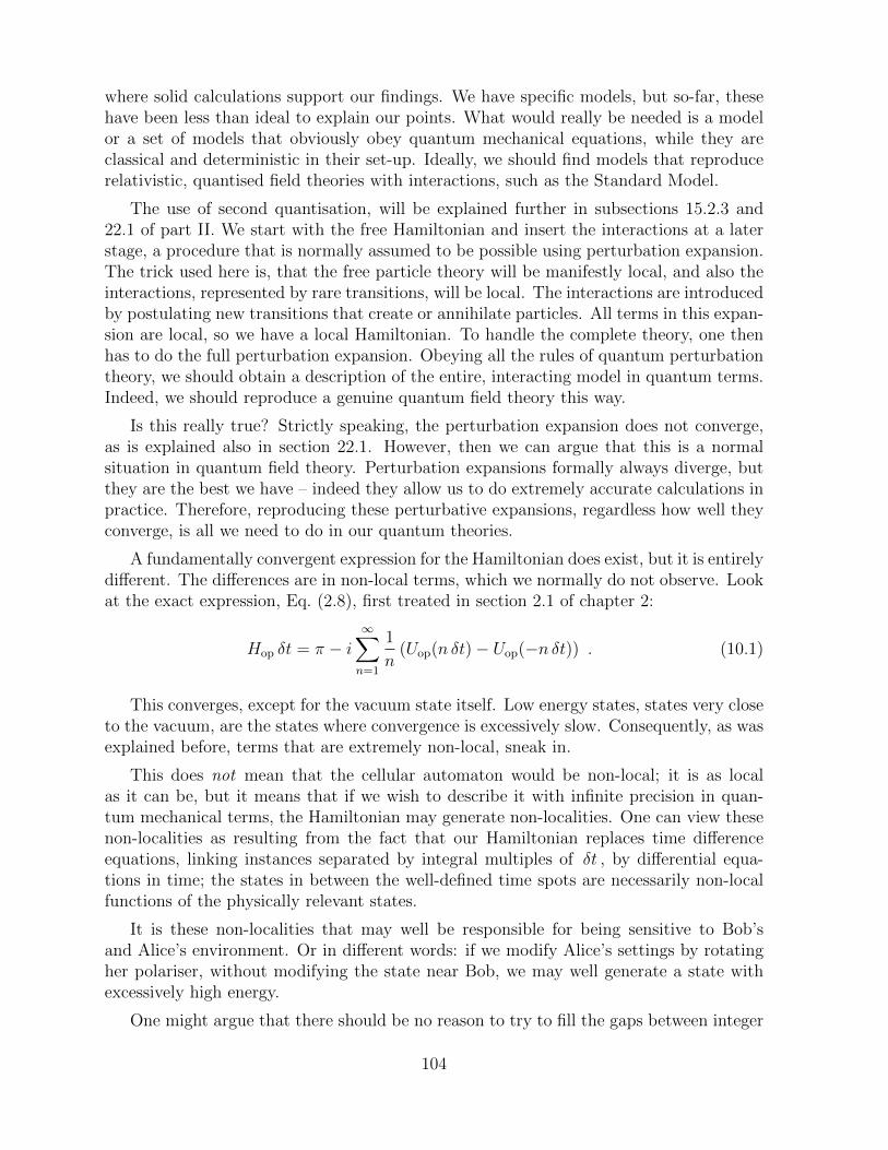
where solid calculations support our findings. We have specific models, but so-far, thesehave been less than ideal to explain our points. What would really be needed is a modelor a set of models that obviously obey quantum mechanical equations, while they areclassical and deterministic in their set-up. Ideally, we should find models that reproducerelativistic, quantised field theories with interactions, such as the Standard Model.

The use of second quantisation, will be explained further in subsections 15.2.3 and22.1 of part II. We start with the free Hamiltonian and insert the interactions at a laterstage, a procedure that is normally assumed to be possible using perturbation expansion.The trick used here is, that the free particle theory will be manifestly local, and also theinteractions, represented by rare transitions, will be local. The interactions are introducedby postulating new transitions that create or annihilate particles. All terms in this expan-sion are local, so we have a local Hamiltonian. To handle the complete theory, one thenhas to do the full perturbation expansion. Obeying all the rules of quantum perturbationtheory, we should obtain a description of the entire, interacting model in quantum terms.Indeed, we should reproduce a genuine quantum field theory this way.

Is this really true? Strictly speaking, the perturbation expansion does not converge,as is explained also in section 22.1. However, then we can argue that this is a normalsituation in quantum field theory. Perturbation expansions formally always diverge, butthey are the best we have – indeed they allow us to do extremely accurate calculations inpractice. Therefore, reproducing these perturbative expansions, regardless how well theyconverge, is all we need to do in our quantum theories.

A fundamentally convergent expression for the Hamiltonian does exist, but it is entirelydifferent. The differences are in non-local terms, which we normally do not observe. Lookat the exact expression, Eq. (2.8), first treated in section 2.1 of chapter 2:

Hop δt = π − i∞∑n=1

1

n(Uop(n δt)− Uop(−n δt)) . (10.1)

This converges, except for the vacuum state itself. Low energy states, states very closeto the vacuum, are the states where convergence is excessively slow. Consequently, as wasexplained before, terms that are extremely non-local, sneak in.

This does not mean that the cellular automaton would be non-local; it is as localas it can be, but it means that if we wish to describe it with infinite precision in quan-tum mechanical terms, the Hamiltonian may generate non-localities. One can view thesenon-localities as resulting from the fact that our Hamiltonian replaces time differenceequations, linking instances separated by integral multiples of δt , by differential equa-tions in time; the states in between the well-defined time spots are necessarily non-localfunctions of the physically relevant states.

It is these non-localities that may well be responsible for being sensitive to Bob’sand Alice’s environment. Or in different words: if we modify Alice’s settings by rotatingher polariser, without modifying the state near Bob, we may well generate a state withexcessively high energy.

One might argue that there should be no reason to try to fill the gaps between integer

104

times steps, but then there would not exist an additive energy function, which we needto stabilise the solutions of or equations. Possibly, we have to use a combination of aclassical, integer-valued Hamilton function (chapter 19 of part II ), and the periodicallydefined Hamiltonian linking only integer-valued time steps, but exactly how to do thiscorrectly is still under investigation. We have not yet found the best possible approachtowards constructing the desired Hamilton operator for our template states. The second-quantised theory that will be further discussed is presently our best attempt, but we havenot yet been able to reproduce the quite complex symmetry structure of the StandardModel, in particular Poincare invariance.

As long as we have no explicit model that, to the extent needed, reproduces StandardModel-like interactions, we cannot verify the correctness of our approach. Lacking that,what has to be done next is the calculations in models that are as realistic as possible.

Part II

Calculation Techniques

11. Introduction to part II

Many of the technical calculations and arguments mentioned in part I of this book, werepostponed to the second part, so as to make the first part easier to read while keeping itcoherent, and to give some nice firework in the second part. The price we pay for this isthat there will be a number of repetitions, for which we apologise.

11.1. Outline of part II

One of our main themes is that quantum mechanics may be viewed as a mathematical toolrather than a new theory of physical phenomena. Indeed, in condensed matter theory,several models exist where the physical setup and the questions asked are fundamen-tally classical, yet the calculations are performed by regarding the system as a quantummechanical one. The Ising Model is a beautiful example of this.[9]

There is no better way to illustrate our approach than by actually showing how suchcalculations are done. The Cogwheel Model was already introduced in section 2.2. Now,in chapters 12.1—13, we show some more of our mathematical tools, how to constructquantum Hamiltonians and how to approach continuum limits. Here, the cogwheel modelis linked to the harmonic rotator, but also other, notoriously ‘classical’ structures, such asthe planetary system, are transformed into models that appear to be quantum mechanical.

105

The continuum limit of a single, periodic cogwheel is an important example. It ap-proaches the ordinary quantum harmonic oscillator with the same period T . The con-tinuum cogwheel is actually a smoothly rotating wheel. Is the classical rotating wheelequivalent to a quantum harmonic oscillator? In a sense, yes, but there are some sub-tleties that one has to be aware of. This is why we decided to do this limit in two steps:first transform the cogwheel into a harmonic rotator, allowing the teeth to form a repre-sentation of the group SU(2) , and only then consider the continuum limit. This enablesus to recognise the operators x and p of a genuine harmonic oscillator already in finitecogwheels.

Like other technical calculations elsewhere in this book, they were done on orderto check the internal consistency of the systems under study. It was fun to do thesecalculations, but they are not intended to discourage the reader. Just skip them, if youare more interested in the general picture.

The issue of the locality of the Hamiltonian is further treated in chapter 14. It willcome up frequently in almost any deterministic model, and again the mathematics isinteresting. We observe that a lot depends on the construction of the vacuum state. It isthe state of lowest energy, and the solution of the equation “energy = lowest”, generatesnon-localities indeed. In reality, as is well known in quantum field theories, signals will notgo faster than the speed of light. What will be shown in this chapter is that there is a wayto avoid non-localities when objects move around surrounded by a vacuum, provided oneuses a first-quantised theory where only the center part of the energy spectrum is used.Consequently, energy can be positive or negative there. Subsequently, one introduces anti-particles, such that the negative energy states actually represent holes of antiparticles. Itis nothing but Dirac’s trick to ensure that the physical vacuum has lowest possible energy.

Dirac first phrased his theory for fermionic particles. Indeed, fermions are easier tounderstand in this respect that bosons are. Therefore, we first introduce fermions as anessential element in our models, see chapter 15.

It so happens that Dirac’s equation for the electron is well suited to demonstrate ourprescription of searching for “beables” in a quantum theory. Section 15.2 also begins atan easy pace but ends up in lengthy derivations. Here also, the reader is invited to enjoythe intricate features of the ‘neutrino’ model, but they can just as well be skipped.

We take the simplified case of the Dirac equation for a two-component neutrino. Itis fundamentally simpler than the Dirac equation for the electron. Furthermore, weassume the absence of interactions. The math starts out simple, but the result is striking:neutrinos are configurations of flat membranes, or ‘sheets’, rather than particles. thesheets move around classically. This is not a theory but a mathematical fact, as long aswe keep mass terms and interactions out of the picture; these are left for later.

Having observed this, we asked the question how to go from the sheet variables back tothe neutrino’s quantum operators such as position ~x , momentum ~p , and spin ~σ . Here,the math does become complicated, and it is interesting as an exercise (subsections 15.2.1and 15.2.2). The neutrinos are ideal for the application of second quantisation (subsection15.2.3), although, in this language, we cannot yet introduce interactions for them.

106

Our models, discussed in chapters 12–17 and 19, have in common that they are local,realistic, and based on conventional procedures in physics. They also have in commonthat they are limited in scope, they do not capture all features known to exist in thereal world, such as all particle species, all symmetry groups, and in particular special andgeneral relativity. The models should be utterly transparent, they indicate directions thatone should look at, and, as was our primary goal, they suggest a great approach towardsinterpreting the quantum mechanical laws that are all so familiar to us.

PQ theory, chapter 16 is a first attempt to understand links between theories based onreal numbers and theories based on integer, or discrete, numbers. The idea is to set up aclean formalism connecting the two, so that it can be used in many instances. Chapter 16also shows some nice mathematical features, with good use of the elliptic theta functions.The calculations look more complicated than they should be, just because we searchedfor an elegant mechanism relating the real line to pairs of integers on the one hand andthe torus on the other, keeping the symmetry between coordinates and momenta.

In chapter 17, we found some other interesting extensions of what was done in chap-ter 16. A very straightforward argument drew our interest to String Theory and Super-string Theory. We are not strongly advocating the idea that the only way to do interestingphysics at the Planck scale is to believe what string theoreticians tell us. It is not clearfrom our work that such theories are the way to go, but we do notice that our programshows remarkable links with string theory. In the absence of interactions, the local equa-tions of string- and superstring theory appear to allow the construction of beables, exactlyalong the route that we advocate. The most striking feature exposed here, is that strings,written in the usual form of continuous quantum field theories in one space, and one timedimension, map onto classical string theories that are not defined in a continuous targetspace, but on a space-time lattice, where the lattice spacing a is given as a = 2π

√α′ .

Symmetries, discussed in chapter 18, are difficult to understand in the CA Interpre-tation of quantum mechanics. However, in the CAI, symmetry considerations are asimportant as anywhere else in physics. Most of our symmetries are discrete, but in somecases, notably in string theory, continuous symmetries such as the Poincare group, canbe recovered.

In chapter 19, we address the positivity problem of the Hamiltonian from a differentperspective. There, the usual Hamiltonian formalism is extended to include discretevariables, again in pairs Pi, Qi , evolving in discrete time. When we first tried to studythis, it seemed like a nightmare, but it so happens that the ‘discrete Hamilton formalism’comes out to be almost as elegant as the usual differential form. And indeed here, theHamiltonian can easily be chosen to be bounded from below.

Eventually, we wish to reproduce effective laws of Nature that should take the form oftoday’s quantum field theories. This is still quite difficult. It was the reason for setting upour procedures in a formal way, so that we will keep the flexibility to adapt our systemsto what Nature seems to be telling us through the numerous ingenious experiments thathave been performed. We explain some of the most important features of quantum fieldtheory in chapter 20. Most notably: in quantum field theories, no signal can carryuseful information faster than the speed of light, and probabilities always add up to one.

107

Quantum field theory is entirely local, in its own inimitable quantum way. These featureswe would like to reproduce in a deterministic quantum theory.

To set up the Cellular Automaton Interpretation in more detail, we first elaboratesome technical issues in cellular automata in general (chapter 21). These are not thetechnicalities encountered when computer programs are written for such systems; softwareexperts will not understand much of our analysis. This is because we are aiming atunderstanding how such systems may generate quantum mechanics at the very largetime and distance limit, and how we may be able to connect to elementary particlephysics. What we find is a beautiful expression for a quantum Hamiltonian, in terms ofan expansion called the BCH expansion. Everything would have been perfect if this werea convergent expansion.

However, it is easy to see that the expansion is not convergent. We try a number ofalternative approaches with some modest successes, but not all issues will be resolved,and the suspicion is aired concerning the source of our difficulties: quantum gravitationaleffects may be of crucial importance, while it is exactly these effects that are still notunderstood as well as is needed here. We do propose to use the BCH expansion for manyclasses of cellular automata to demonstrate how they could be used to interpret quantummechanics. I know that the details are not yet quite right, but this probably has to beattributed to the simple fact that we left out lots of things, notably special and generalrelativity

11.2. Notation

It is difficult keep our notation completely unambiguous. In chapter 16, we are dealingwith many different types of variables and operators. When a dynamical variable is aninteger there, we shall use capitals A, B, · · · , P, Q, · · · . Variables that are periodic withperiod 2π , or at least constrained to lie in an interval such as (−π, π] , are angles, mostlydenoted by Greek lower case letters α, β, · · · , κ, θ, · · · , whereas real variables will mostoften be denoted by lower case Latin letters a, b, · · · , x, y, · · · . Yet sometimes we run outof symbols and deviate from this scheme, if it seems to be harmless to do so. For instance,indices will still be i, j, · · · for space-like vector components, α, β, · · · for spinors andµ, ν, · · · for Lorentz indices. The Greek letters ψ and ϕ will be used for wave functionsas well.

Yet it is difficult to keep our notation completely consistent; in some chapters beforechapter 16, we use the quantum numbers ` and m of the SU(2) representations todenote the integers that earlier were denoted as k or k − m , and later in chapter 16replaced by capitals.

As in part I, we use a super- or subscript “op” to distinguish an operator from anordinary numerical variable. The caret ( ) will be reserved for vectors with length one,the arrow for more general vectors, not necessarily restricted to three dimensional space.Only in chapter 20, where norms of vectors do not arise, we use the caret for the Fouriertransform of a function.

108

Dirac’s constant ~ and the velocity of light c will nearly always be defined to be onein the units chosen. In previous work, we used a spacial symbol to denote e2π as analternative basis for exponential functions. This would indeed sometimes be useful forcalculations, when we use fractions that lie between 0 and 1, rather than angles, and itwould require that we normalise Planck’s original constant h rather then ~ to one, butin the present monograph we return to the more usual notation.

Concepts frequently discussed are the following:

- discrete variables are variables such as the integer numbers, whose possible valuescan be counted. Opposed to continuous variables, which are typically representedby real or complex numbers.

- fractional variables are variables that take values in a finite interval or on a circle.The interval may be [0, 1) , [0, 2π) , (−1

2, 1

2] , or (−π, π] . Here, the square bracket

indicates a bound whose value itself may be included, a round bracket excludesthat value. A real number can always be decomposed into an integer (or discrete)number and a fractional one.

- a theory is ontological, or ‘ontic’, if it only describes ‘really existing’ objects; it issimply a classical theory such as the planetary system, in the absence of quantummechanics. The theory does not require the introduction of Hilbert space, although,as will be explained, Hilbert space might be very useful. But then, the theory isformulated in terms of observables that are commuting at all times.

- a feature is counterfactual when it is assumed to exist even if, for fundamentalreasons, it cannot actually be observed; if one would try to observe it, some otherfeature might no longer be observable and hence become counterfactual. This sit-uation typically occurs if one considers the measurement of two or more operatorsthat do not commute. More often, in our models, we shall encounter features thatare not allowed to be counterfactual.

- We talk of templates when we describe particles and fields as solutions of Schro-dinger’s equation in an ontological model, as was explained in subsection 4.3.1.Templates may be superpositions of ontic states and/or other templates, but theontic states all form an orthonormal set; superpositions of ontic states are neverontic themselves.

11.3. More on Dirac’s notation for quantum mechanics

A denumerable set of states |ei〉 is called an orthonormal basis of H if every state |ψ〉 ∈ Hcan be approximated by a linear combination of a finite number of states |ei〉 up to anyrequired precision:

|ψ〉 =

N(ε)∑i=1

λi|ei〉+ |ε〉 , ‖ε‖2 = 〈ε|ε〉 < ε2 , for any ε > 0 . (11.1)

109

(a property called ‘completeness’), while

〈ei|ej〉 = δij (11.2)

(called ‘orthonormality’). From Eqs. (11.1) and (11.2), one derives

λi = 〈ei|ψ〉 ,∑i

|ei〉〈ei| = I , (11.3)

where I is the identity operator: I|ψ〉 = |ψ〉 for all |ψ〉 .In many cases, the discrete sum in Eqs. (11.1) and (11.3) will be replaced by an

integral, and the Kronecker delta δij in Eq. (11.2) by a Dirac delta function, δ(x1− x2) .We shall still call the states |e(x)〉 a basis, although it is not denumerable.

A typical example is the set of wave functions ψ(~x) describing a particle in positionspace. They are regarded as vectors in Hilbert space where the set of delta peak wavefunctions |~x〉 is chosen to be the basis:

ψ(~x) ≡ 〈~x|ψ〉 , 〈~x|~x ′〉 = δ3(~x− ~x ′) . (11.4)

The Fourier transformation is now a simple rotation in Hilbert space, or a transition tothe momentum basis :

〈~x|ψ〉 =

∫d3~p 〈~x|~p 〉〈~p |ψ〉 ; 〈~x|~p 〉 = 1

(2π)3/2ei~p·~x . (11.5)

Many special functions, such as the Hermite, Laguerre, Legendre, and Bessel functions,may be seen as generating different sets of basis elements of Hilbert space.

Often, we use product Hilbert spaces: H1 ⊗ H2 = H3 , which means that states |φ〉in H3 can be seen as normal products of states |ψ(1)〉 in H1 and |ψ(2)〉 in H2 :

|φ〉 = |ψ(1)〉|ψ(2)〉 , (11.6)

and a basis for H3 can be obtained by combining a basis in H1 with one in H2 :

|e(3)ij 〉 = |e(1)

i 〉|e(2)j 〉 . (11.7)

Often, some or all of these factor Hilbert spaces are finite-dimensional vector spaces,which of course also allow all the above manipulations30. We have, for example, the 2-dimensional vector space spanned by spin 1

2particles. A basis is formed by the two states

| ↑ 〉 and | ↓ 〉 . In this basis, the Pauli matrices σop1,2,3 are defined as in part I, Eqs. 1.7.

The states

| → 〉 = 1√2

(11

), | ← 〉 = 1√

2

(1−1

), (11.8)

30The term Hilbert space is often restricted to apply to infinite dimensional vector spaces only; here wewill also include the finite dimensional cases.

110

form the basis where the operator σ1 is diagonal: σop1 →

(1 00 −1

).

Dirac derived the words ‘bra’ and ‘ket’ from the fact that the expectation value for anoperator Oop can be written as the operator between brackets, or

〈Oop〉 = 〈ψ| Oop|ψ〉 . (11.9)

More generally, we shall often need the matrix elements of an operator in a basis |ei〉 :

Oij = 〈ei|Oop|ej〉 . (11.10)

The transformation from one basis |ei〉 to another, |e′i〉 is a unitary operator Uij :

|e′i〉 =∑j

Uij|ej〉 , Uij = 〈ej|e′i〉 ;∑k

UikUjk =∑k

〈e′i|ek〉〈ek|e′j〉 = δij . (11.11)

This will be used frequently. For instance, the Fourier transform is unitary:∫d3~p 〈~x|~p 〉〈~p |~x′〉 = 1

(2π)3

∫d3~p ei~p·~x−i~p·~x

′= δ3(~x− ~x′) . (11.12)

The Schrodinger equation will be written as:

ddt|ψ(t)〉 = −iHop|ψ(t)〉 , d

dt〈ψ(t)| = 〈ψ(t)|iHop ;

|ψ(t)〉 = e−iHop t|ψ(0)〉 , (11.13)

where Hop is the Hamiltonian, defined by its matrix elements Hij = 〈ei|Hop|ej〉 .Dirac’s notation may be used to describe non-relativistic wave functions in three space

dimensions, in position space, in momentum space or in some other basis, such as a partialwave expansion, it can be used for particles with spin, it can be used in many-particlesystems, and also for quantised fields in solid state theory or in elementary particle theory.The transition from a Fock space notation, where the basis is spanned by states containinga fixed number N of particles (in position or in momentum space, possibly having spinas well), to a notation where the basis is spanned by the functions representing the fieldsof these particles, is simply a rotation in Hilbert space, from one basis into another.

12. More on cogwheels

12.1. the group SU(2) , and the harmonic rotator

Let us return to the original cogwheel with N teeth, as introduced in chapter 2, section2.2. It may be very illuminating to define the constant ` = (N − 1)/2 , and introduce the

111

operators L1, L2 and L3 as follows ( k = 0, 1, · · · , 2 ` is the energy quantum number;the time step is δt = 1 ):

L3 = N2πHop − ` = k − ` ,

L1 = 12(L+ + L−) , L2 = −1

2i (L+ − L−) ,

L+|k〉H =√

(k + 1)(2`− k) |k + 1〉H ,

L−|k〉H =√k(2`+ 1− k) |k − 1〉H . (12.1)

Using the quantum number m = k − ` = L3 , we get the more familiar expressions forthe angular momentum operators La, a = 1, 2, 3, obeying the commutation relations

[La, Lb] = iεabcLc . (12.2)

The original ontological states |n〉ont can be obtained from the angular momentum statesby means of the transformation rules (2.21) and (2.22). It is only these that evolve asontological states. Other operators can be very useful, however. Take, for instance,

x = 1√`L1 , p = − 1√

`L2 , [x, p] = i(1− 2`+1

2π`Hop) , (12.3)

then, for states where the energy 〈Hop〉 1 , we have the familiar commutation rules forpositions x and momenta p , while the relation L2

1 + L22 + L2

3 = L2 = `(` + 1) impliesthat, when 〈Hop〉 1/

√` ,

H → 2πN

12(p2 + x2 − 1) , (12.4)

which is the Hamiltonian for the harmonic oscillator (the zero point energy has beensubtracted, as the lowest energy eigen state was set at the value zero). Also, at lowvalues for the energy quantum number k , we see that L± approach the creation andannihilation operators of the harmonic oscillator (see Eqs. (12.1)):

L− →√

2`+ 1 a , L+ →√

2`+ 1 a† . (12.5)

Thus, we see that the lowest energy states of the cogwheel approach the lowest energystates of the harmonic oscillator. This will be a very useful observation if we wish toconstruct models for quantum field theories, starting from deterministic cogwheels. Themodel described by eqs. (12.1)–(12.3) will be referred to as the harmonic rotator. TheZeeman atom of section 2.2 is a simple example with ` = 1 .

Note, that the spectrum of the Hamiltonian of the harmonic rotator is exactly that ofthe harmonic oscillator, except that there is an upper limit, Hop < 2π . By construction,the period T = (2 ` + 1)δt of the harmonic rotator, as well as that of the harmonicoscillator, is exactly that of the periodic cogwheel.

The Hamiltonian that we associate to the harmonic rotator is also that for a spinningobject that exhibits precession due to a torque force on its axis. Thus, physically, we seethat an oscillator drawing circles in its (x, p) phase space is here replaced by a precessingtop. At the lowest energy levels, they obey the same equations.

112

We conclude from this section that a cogwheel with N states can be regarded as arepresentation of the group SU(2) with total angular momentum ` , and N = 2 `+1 . Theimportance of this approach is that the representation is a unitary one, and that thereis a natural ground state, the ground state of the harmonic oscillator. In contrast to theharmonic oscillator, the harmonic rotator also has an upper bound to its Hamiltonian.The usual annihilation and creation operators, a and a† , are replaced by L− and L+ ,whose commutator is not longer constant but proportional to L3 , and therefore changingsign for states |k〉 with ` < k ≤ 2 ` . This sign change assures that the spectrum isbounded from below as well as above, as a consequence of the modified algebra, (12.2).

12.2. Infinite, discrete cogwheels

Discrete models with infinitely many states may have the new feature that some orbitsmay not be periodic. They then contain at least one non-periodic ‘rack’. There existsa universal definition of a quantum Hamiltonian for this general case, though it is notunique. Defining the time reversible evolution operator over the smallest discrete timestep to be an operator Uop(1) , we now construct the simplest Hamiltonian Hop suchthat Uop(1) = e−iHop . For this, we use the evolution over n steps, where n is positiveor negative:

Uop(n) = Uop(1)n = e−inHop . (12.6)

Let us assume that the eigenvalues ω of this Hamiltonian lie between 0 and 2π . We canthen consider the Hamiltonian in the basis where both U(1) and H are diagonal. Write

e−inω = cos(nω)− i sin(nω) , (12.7)

and then use Fourier transformations to derive that, if −π < x < π ,

x = 2∞∑n=1

(−1)n−1 sin(nx)

n. (12.8)

Next, write Hop = ω = x+ π , to find that Eq. (12.8) gives

ω = π − 2∞∑n=1

sin(nω)

n. (12.9)

Consequently, as in Eq. (2.8),

ω = π −∞∑n−1

i

n(U(n δt)− U(−n δt) ) and

Hop = π −∞∑n−1

i

n(Uop(n δt)− Uop(−n δt) ) . (12.10)

Very often, we will not be content with this Hamiltonian, as it has no eigenvalues beyondthe range (0, 2π) . As soon as there are conserved quantities, one can add functions of

113

these at will to the Hamiltonian, to be compared with what is often done with chemicalpotentials. Cellular automata in general will exhibit many such conservation laws. SeeFig. 3, where every closed orbit represents something that is conserved: the label of theorbit.

In section 13, we consider the other continuum limit, which is the limit δt → 0 forthe cogwheel model. First, we look at continuous theories more generally.

12.3. Automata that are continuous in time

In the physical world, we have no direct indication that time is truly discrete. It istherefore tempting to consider the limit δt→ 0 . At first sight, one might think that thislimit should be the same as having a continuous degree of freedom obeying differentialequations in time, but this is not quite so, as will be explained later in this chapter.First, in this section, we consider the strictly continuous deterministic systems. Then, wecompare those with the continuum limit of discrete systems.

Consider an ontological theory described by having a continuous, multi-dimensionalspace of degrees of freedom ~q (t) , depending on one continuous time variable t , and itstime evolution following classical differential equations:

d

dtqi(t) = fi(~q ) , (12.11)

where fi(~q ) may be almost any function of the variables qj .

An example is the description of massive objects obeying classical mechanics in Ndimensions. Let a = 1, · · · , N, and i = 1, · · · , 2N :

i = a ⊕ a+N , qa(t) = xa(t) , qa+N(t) = pa(t) ,

fa(~q ) =∂Hclass(~x, ~p )

∂pa, fa+N(~q ) = −∂Hclass(~x, ~p )

∂xa, (12.12)

where Hclass is the classical Hamiltonian.

An other example is the quantum wave function of a particle in one dimension:

i = x , qi(t) = ψ(x, t) ; fi(~q ) = −iHS ψ(x, t) , (12.13)

where now HS is the Schrodinger Hamiltonian. Note, however, that, in this case, thefunction ψ(x, t) would be treated as an ontological object, so that the Schrodinger equa-tion and the Hamiltonian eventually obtained will be quite different from the Schrodingerequation we start off with; actually it will look more like the corresponding second quan-tised system (see later).

We are now interested in turning Eq. (12.11) into a quantum system by changing thenotation, not the physics. The ontological basis is then the set of states |~q 〉 , obeying theorthogonality property

〈~q |~q ′〉 = δN(~q − ~q ′) , (12.14)

114

where δ is now the Dirac delta distribution, and N is the dimensionality of the vectors~q .

If we wrote

d

dtψ(~q )

?= − fi(~q )

∂

∂qiψ(~q )

?= − iHop ψ(~q ) , (12.15)

where the index i is summed over, we would read off that

Hop?= − ifi(~q )

∂

∂qi= fi(~q )pi , pi = −i ∂

∂qi. (12.16)

This, however, is not quite the right Hamiltonian because it may violate hermiticity:Hop 6= H†op . The correct Hamiltonian is obtained if we impose that probabilities are pre-

served, so that, in case the Jacobian of ~f(~q ) does not vanish, the integral∫

dN~q ψ†(~q )ψ(~q )is still conserved:

d

dtψ(~q = −fi(~q )

∂

∂qiψ(~q )− 1

2

(∂fi(~q )

∂qi

)ψ(~q ) = −iHop ψ(~q ) , (12.17)

Hop = −ifi(~q )∂

∂qi− 1

2i(∂fi(~q )

∂qi

)= 1

2(fi(~q )pi + pifi(~q )) ≡ 1

2fi(~q ), pi . (12.18)

The 1/2 in Eq. (12.17) ensures that the product ψ† ψ evolves with the right Jacobian.Note that this Hamiltonian is hermitean, and the evolution equation (12.11) follows im-mediately from the commutation rules

[qi, pj] = iδij ;d

dtOop(t) = −i[Oop , Hop ] . (12.19)

Now, however, we encounter a very important difficulty: this Hamiltonian has no lowerbound. It therefore cannot be used to stabilise the wave functions. Without lower bound,one cannot do thermodynamics. This feature would turn our model into something veryunlike quantum mechanics as we know it.

If we take ~q space either one-dimensional, or in some cases two-dimensional, we canmake our system periodic. Then let T be the smallest positive number such that

~q (T ) = ~q (0) . (12.20)

We have consequently

e−iHT |~q (0)〉 = |~q(0) 〉 , (12.21)

and therefore, on these states,

Hop |~q 〉 =∞∑

n=−∞

2πn

T|n〉HH〈n|~q 〉 . (12.22)

115

Thus, the spectrum of eigenvalues of the energy eigenstates |n〉H runs over all integersfrom −∞ to ∞ .

In the discrete case, the Hamiltonian has a finite number of eigenstates, with eigenval-ues 2πk/(Nδt) + δE where k = 0, · · · , N − 1 , which means that they lie in an interval[δE , 2π/T + δE] , where T is the period, and δE can be freely chosen. So here, wealways have a lower bound, and the state with that energy can be called ‘ground state’or ‘vacuum’.

Depending on how the continuum limit is taken, we may or may not preserve thislower bound. The lower bound on the energy seems to be artificial, because all energyeigenstates look exactly alike. It is here that the SU(2) formulation for harmonic rotators,handled in subsection 12.1, may be hore useful

An other remedy against this problem could be that we demand analyticity when timeis chosen to be complex, and boundedness of the wave functions in the lower half of thecomplex time frame. This would exclude the negative energy states, and still allow usto represent all probability distributions with wave functions. Equivalently, one couldconsider complex values for the variable(s) ~q and demand the absence of singularities inthe complex plane below the real axis. Such analyticity constraints however seem to berather arbitrary; they are difficult to maintain as soon as interactions are introduced, sothey would certainly have to be handled with caution.

One very promising approach to solve the ground state problem is Dirac’s great ideaof second quantisation: take an indefinite number of objects ~q , that is, a Hilbert spacespanned by all states |~q (1), ~q (2), · · · ~q (n)〉 , for all particle numbers n , and regard thenegative energy configurations as ‘holes’ of antiparticles. This we propose to do in our‘neutrino model’, section 15.2, and in later chapters.

Alternatively, we might consider the continuum limit of a discrete theory more care-fully. This we try first in the next chapter. Let us emphasise again: in general, excisingthe negative energy states just like that is not always a good idea, because any pertur-bation of the system might cause transitions to these negative energy states, and leavingthese transitions out may violate unitarity.

The importance of the ground state of the Hamiltonian was discussed in chapter 9 ofpart I. The Hamiltonian (12.18) is an important expression for fundamental discussionson quantum mechanics.

As in the discrete case, also in the case of deterministic models with a continuousevolution law, one finds discrete and continuous eigenvalues, depending on whether or nota system is periodic. In the limit δt → 0 of the discrete periodic ontological model, theeigenvalues are integer multiples of 2π/T , and this is also the spectrum of the harmonicoscillator with period T , as explained in chapter 13. The harmonic oscillator may beregarded as a deterministic system in disguise.

The more general continuous model is then the system obtained first by having a(finite or infinite) number of harmonic oscillators, which means that our system consistsof many periodic substructures, and secondly by admitting a (finite or infinite) numberof conserved quantities on which the periods of the oscillators depend. An example is

116

the field of non-interacting particles; quantum field theory then corresponds to havingan infinite number of oscillating modes of this field. The particles may be fermionic orbosonic; the fermionic case is also a set of oscillators if the fermions are put in a box withperiodic boundary conditions. Interacting quantum particles will be encountered later(chapter 19 and onwards).

13. The continuum limit of cogwheels, harmonic rotators andoscillators

In the N →∞ limit, a cogwheel will have an infinite number of states. The Hamiltonianwill therefore also have infinitely many eigenstates. We have seen that there are two waysto take a continuum limit. As N → ∞ , we can keep the quantised time step fixed,say it is 1. Then, in the Hamiltonian (2.24), we have to allow the quantum number kto increase proportionally to N , keeping κ = k/N fixed. Since the time step is one,the Hamiltonian eigenvalues, 2πκ , now lie on a circle, or, we can say that the energytakes values in the continuous line segment [0, 2π) (including the point 0 but excludingthe point 2π ). Again, one may add an arbitrary constant δE to this continuum ofeigenvalues. What we have then, is a model of an object moving on a lattice in onedirection. At the beat of a clock, a state moves one step at a time to the right. This is therack, introduced in section 12.2. The second-quantised version is handled in section 17.1.

The other option for a continuum limit is to keep the period T of the cogwheelconstant, while the time quantum δt tends to zero. This is also a cogwheel, now withinfinitely many, microscopic teeth, but still circular. Since now N δt = T is fixed, theontological31 states of the system can be described as an angle:

2πn/N → ϕ ,d

dtϕ(t) =

2π

T. (13.1)

The energy eigenvalues become

Ek = 2π k/T + δE , k = 0, 1, · · · , ∞ . (13.2)

If δE is chosen to be π/T , we have the spectrum Ek = (2π/T )(k + 12) . This is the

spectrum of a harmonic oscillator. In fact, any periodic system with period T , anda continuous time variable can be characterised by defining an angle ϕ obeying theevolution equation (13.1), and we can attempt to apply a mapping onto a harmonicoscillator with the same period.

Mappings of one model onto another one will be frequently considered in this book.It will be of importance to understand what we mean by this. If one does not put anyconstraint on the nature of the mapping, one would be able to map any model onto anyother model; physically this might then be rather meaningless. Generally, what we arelooking for are mappings that can be prescribed in a time-independent manner. This

31The words ‘ontological’ and ‘deterministic’ will be frequently used to indicate the same thing: amodel without any non deterministic features, describing things that are really there.

117

means that, once we know how to solve the evolution law for one model, then afterapplying the mapping, we have also solved the evolution equations of the other model.The physical data of one model will reveal to us how the physical data of the other oneevolve.

This requirement might not completely suffice in case a model is exactly integrable. Inthat case, every integrable model can be mapped onto any other one, just by consideringthe exact solutions. In practice, however, time independence of the prescription can beeasily verified, and if we now also require that the mapping of the physical data of onemodel onto those of the other is one-to-one, we can be confident that we have a relationof the kind we are looking for. If now a deterministic model is mapped onto a quantummodel, we may demand that the classical states of the deterministic model map ontoan orthonormal basis of the quantum model. Superpositions, which look natural in thequantum system, might look somewhat contrived and meaningless in the deterministicsystem, but they are certainly acceptable as describing probabilistic distributions in thelatter. This book is about these mappings.

We have already seen how a periodic deterministic system can produce a discrete spec-trum of energy eigenstates. The continuous system described in this subsection generatesenergy eigenstates that are equally spaced, and range from a lowest state to E → ∞ .Mapping this onto the harmonic oscillator, seems to be straightforward; all we have todo is map these energy eigenstates onto those of the oscillator, and since these are alsoequally spaced, both systems will evolve in the same way. Of course this is nothing to besurprised about: both systems are integrable and periodic with the same period T .

For the rest of this subsection, we will put T = 2π . The Hamiltonian of this harmonicoscillator can then be chosen to be32

Hop = 12(p2 + x2 − 1) ; Hop |n〉H = n |n〉H , n = 0, 1, · · · ,∞ . (13.3)

The subscript H reminds us that we are looking at the eigenstates of the HamiltonianHop . For later convenience, we subtracted the zero point energy33.

In previous versions of this book’s manuscript, we described a mapping that goesdirectly from a deterministic (but continuous) periodic system onto a harmonic oscillator.Some difficulties were encountered with unitarity of the mapping. At first sight, thesedifficulties seemed not to be very serious, although they made the exposition less thantransparent. It turned out, however, that having a lower bound but not an upper boundon the energy spectrum does lead to pathologies that we wish to avoid.

It is much better to do the mapping in two steps: have as an intermediate model theharmonic rotator, as was introduced in chapter 12.1. The harmonic rotator differs fromthe harmonic oscillator by having not only a ground state, but also a ceiling. This makesit symmetric under sign switches of the Hamiltonian. The lower energy domain of the

32In these expressions, x, p, a , and a† are all operators, but we omitted the subscript “op” to keepthe expressions readable.

33Interestingly, this zero point energy would have the effect of flipping the sign of the amplitudes afterexactly one period. Of course, this phase factor is not directly observable, but it may play some role infuture considerations. In what we do now, it is better to avoid these complications.

118

rotator maps perfectly onto the harmonic oscillator, while the transition from the rotatorto the continuous periodic system is a straightforward limiting procedure.

Therefore, let us first identify the operators x and p of the harmonic rotator, withoperators in the space of the ontological states |ϕ〉ont of our periodic system. This isstraightforward, see Eqs. (12.3). In the energy basis of the rotator, we have the loweringoperator L− and the raising operator L+ which give to the operators x and p thefollowing matrix elements between eigenstates |m〉 , −` ≤ m ≤ ` , of Hop :

〈m− 1|x|m〉 = 12

√(m+`)(`+1−m)

`= 〈m|x|m− 1〉 ,

〈m− 1|p|m〉 = 12i√

(M+`)(`+1−m)`

= −〈m|p|m− 1〉 , (13.4)

while all other matrix elements vanish.

13.1. The operator ϕop in the harmonic rotator

As long as the harmonic rotator has finite ` , the operator ϕop is to be replaced by adiscrete one:

ϕop =2π

2`+ 1σ , σ = −` , −`+ 1 , · · · , +` . (13.5)

By discrete Fourier transformations, one derives that the discrete function ϕ(σ) obeysthe finite Fourier expansion,

σ = i2∑k=1

(−1)k

2 sin(πk

2`+1

) e2πikσ2`+1 . (13.6)

By modifying some phase factors, we replace the relations (2.21) and (2.22) by

|m〉H ≡ 1√2`+ 1

∑σ=−`

e2πimσ2`+1 |σ〉ont , (13.7)

|σ〉ont =1√

2`+ 1

∑m=−`

e−2πimσ

2`+1 |m〉H (13.8)

(which symmetrizes the Hamiltonian eigenvalues m , now ranging from −` to ` ).

One now sees that the operator e2πi

2`+1σ

increases the value m by one unit, with theexception of the state |m = `〉 , which goes to |m = −`〉 . Therefore,

e2πiσ2`+1 = (`+ 1−H)−1/2 L+ (`+ 1 +H)−1/2 + | − ` 〉〈 ` | ;

e−2πiσ2`+1 = (`+ 1 +H)−1/2 L− (`+ 1−H)−1/2 + | ` 〉〈−` | , (13.9)

119

and Eq. (13.6) can now be written as

〈m+ k|σ|m〉 =i(−1)k

2 sin(πk

2`+1

) , k 6= 0 ,

〈m|σ|m〉 = 0 . (13.10)

Eqs (13.9) can easily be seen to be unitary expressions, for all ` in the harmonic rotator.Care was taken to represent the square roots in the definitions of L± correctly: sincenow |H| ≤ ` , one never encounters division by 0. The quantity m + k characterisingthe state in Eq. (13.10) must be read Modulo 2` + 1 , while observing the fact that forhalf-odd-integer values of ` the relations (13.7) and (13.8) are both anti periodic withperiod 2`+ 1 .

The operator σ in Eqs (13.9) and (13.10) can now be seen to evolve deterministically:

σ(t) = σ(0) + (2`+ 1) t/T . (13.11)

The eigenstates |ϕ〉 of the operator ϕop are closely related to Glauber’s coherentstates in the harmonic oscillator [17], but our operator ϕop is hermitean and its eigen-states are orthonormal; Glauber’s states are eigenstates of the creation or annihilationoperators, which were introduced by him following a different philosophy. Orthonormal-ity is a prerequisite for the ontological states that are used in this work.

13.2. The harmonic rotator in the x frame

In harmonic oscillators, it is quite illuminating to see how the equations look in thecoordinate frame. The energy eigen states are the Hermite functions. It is an interestingexercise in mathematical physics to investigate how the ontological operator (beable) ϕop

can be constructed as a matrix in x -space. As was explained at the beginning of thischapter however, we refrain from exhibiting this calculation as it might lead to confusion.

The operator ϕop is represented by the integer σ in Eq. (13.5). This operator istransformed to the energy basis by Eqs. (13.7) and (13.8), taking the form (13.9). Inorder to transform these into x space, we first need the eigen states of Lx in the energybasis. This is a unitary transformation requiring the matrix elements 〈m3|m1〉 , wherem3 are the eigen values of L3 and m1 those of Lx . Using the ladder operators L± , onefinds the useful recursion relation

2m1〈m1|m3〉 =√

(`+m3 + 1)(`−m3) 〈m1|m3 + 1〉 +√(`+m3)(`+ 1−m3) 〈m1|m3 − 1〉 , (13.12)

First remove the square roots by defining new states ||m3〉 and ||m1〉 :

||m3〉 ≡√

(`+m3)! (`−m3)! |m3〉 ,||m1〉 ≡

√(`+m1)! (`−m1)! |m1〉 . (13.13)

120

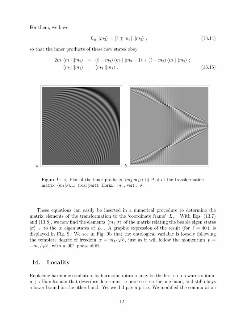
For them, we have

L± ||m3〉 = (`∓m3) ||m3〉 , (13.14)

so that the inner products of these new states obey

2m1〈m1|||m3〉 = (`−m3) 〈m1|||m3 + 1〉+ (`+m3) 〈m1|||m3〉 ;

〈m1|||m3〉 = 〈m3|||m1〉 . (13.15)

a. b.

Figure 9: a) Plot of the inner products 〈m3|m1〉 ; b) Plot of the transformationmatrix 〈m1|σ〉ont (real part). Horiz.: m1 , vert.: σ .

These equations can easily be inserted in a numerical procedure to determine thematrix elements of the transformation to the ‘coordinate frame’ Lx . With Eqs. (13.7)and (13.8), we now find the elements 〈m1|σ〉 of the matrix relating the beable eigen states|σ〉ont to the x eigen states of Lx . A graphic expression of the result (for ` = 40 ), isdisplayed in Fig. 9. We see in Fig. 9b that the ontological variable is loosely followingthe template degree of freedom x = m1/

√` , just as it will follow the momentum p =

−m2/√` , with a 90 phase shift.

14. Locality

Replacing harmonic oscillators by harmonic rotators may be the first step towards obtain-ing a Hamiltonian that describes deterministic processes on the one hand, and still obeysa lower bound on the other hand. Yet we did pay a price. We modified the commutation

121

rules between the coordinate operators called x and the momentum operators p . If wewould apply this to field theories, we would find it difficult to decompose the fields intoharmonic modes. These modes would no longer commute with one another, and thatwould constitute a serious blow to the concept of locality.

We have also seen how a Hamiltonian can be constructed starting off from just anydeterministic system, including systems that are entirely local in the usual sense. If timeis continuous, that Hamiltonian tends to take the form of Eq, (12.18), which has neither alower nor an upper bound, but it does seem to be local. In contrast, the Hamiltonians ofthe discrete-time models, such as Eqs. (2.8), (2.26), (2.27), and (12.10), have in commonthat they are bounded, but they are expressed in terms of the evolution operators atfairly large times t = nδt . For cellular automaton models, discussed in section 5.1and chapter 21, the evolution operator over n time steps, involves interactions amongneighbours that are n space-steps apart. If, instead, we wish to restrict ourselves to localexpressions, this means that a cut-off will have to be introduced when defining H , butthis is only allowed if the sums in question converge sufficiently rapidly. It seems to bethe combination of the positivity requirement and the locality requirement that is oftendifficult to obey.

Can this conflict be avoided? Should we search for different models, or should wesearch for different approximation methods in all models we are using? The author’spresent understanding is, that we will have to put constraints on the models to which wecan apply our theories. Different models will be discussed later (section 9.2). Let us hereconcentrate on the nature of the conflict.

In part I, section 2.1, we introduced the concept of the templates. Let us see whathappens when we impose a further constraint on the templates: Consider only thosetemplate states that are slowly varying in time. We assume that the time dependence inthe templates is much slower than the fundamental time interval δt in the ontologicalevolution law. This means that we consider only those elements of Hilbert space wherethe eigenvalue E of H lies in an interval |E| ≤ 1

2Λ , or, when we add our free constant

to the energy levels, we impose

0 ≤ E ≤ Λ . (14.1)

States composed as superpositions of these energy eigenvalues will show probabilities|〈ont|ψ(t)〉|2 whose time dependence only contains terms eiωt with |ω| ≤ Λ . Templatesobeying Ineq. (14.1) will be referred to as slow templates.

It is advised, however, to be reserved in the use of slow templates; in classical states,energies can easily reach values above the Planck energy (the kinetic energy of a smallpassenger airplane at cruise speed), and these would require faster templates.

Figure 10 a shows the approximation obtained for the Hamiltonian, in the case we usethe expansion (2.8), with a smooth cut-off. We introduced a suppression factor e−k/R forthe kth term (in the Figure, R = 30 ). What happens when we use this approximationfor the Hamiltonian?

First, it is not quite local anymore. In a cellular automaton, where we have onlynearest neighbour interactions, the Hamiltonian will feature ‘ghost interactions’ between

122

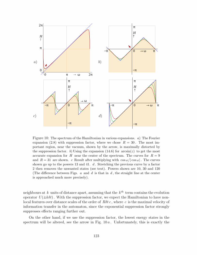
a)

0 π 2πω0

π

2π

H

b)

−π 0 πω

H

π

−π

c)

−π 0 πω

H

π

−π

d)

−π 0 πω

H

π

−π

Figure 10: The spectrum of the Hamiltonian in various expansions. a) The Fourierexpansion (2.8) with suppression factor, where we chose R = 30 . The most im-portant region, near the vacuum, shown by the arrow, is maximally distorted bythe suppression factor. b) Using the expansion (14.6) for arcsin(z) to get the mostaccurate expansion for H near the center of the spectrum. The curves for R = 9and R = 31 are shown. c Result after multiplying with cosω/| cosω| . The curvesshown go up to the powers 13 and 41. d . Stretching the previous curve by a factor2 then removes the unwanted states (see text). Powers shown are 10, 30 and 120(The difference between Figs. a and d is that in d , the straight line at the centeris approached much more precisely).

neighbours at k units of distance apart, assuming that the kth term contains the evolutionoperator U(±kδt) . With the suppression factor, we expect the Hamiltonian to have non-local features over distance scales of the order of Rδt c , where c is the maximal velocity ofinformation transfer in the automaton, since the exponential suppression factor stronglysuppresses effects ranging further out.

On the other hand, if we use the suppression factor, the lowest energy states in thespectrum will be altered, see the arrow in Fig. 10 a . Unfortunately, this is exactly the

123

physically most important region, near the vacuum state (the lowest energy state). It isnot difficult to estimate the extent of the deformation close to the origin. The sum withcut-off can be evaluated exactly. For large values of the cut-off R , and 0 < ω < π , theapproximation ωapprox for the true eigenvalues ω of the Hamiltonian will be:

ωapprox = π − 2∞∑n=1

sin(nω)e−n/R

n= 2 arctan

(e1/R − cosω

sinω

)= 2 arctan

(1− cosω + 1/Rsinω

)= 2 arctan

( sinω

1 + cosω+

1/Rsinω

), (14.2)

where we replaced e1/R by 1 + 1/R since R is large and arbitrary.

Writing sinα1+cosα

= tan 12α , we see that the approximation becomes exact in the limit

R→∞ . We are interested in the states close to the vacuum, having a small but positiveenergy H = α . Then, at finite R , the cut-off at R replaces the eigenvalues H of theHamiltonian Hop by

H → H +2

RH, (14.3)

which has its minimum at H0 ≈√

2/R , where the value of the minimum is H ≈ 2√

2/R .This is only acceptable if

RMPl/〈Hop〉2 . (14.4)

Here, MPl is the “Planck mass”, or whatever the inverse is of the elementary time scalein the model. This cut-off radius R must therefore be chosen to be very large, so that,indeed, the exact quantum description of our local model generates non-locality in theHamiltonian.

Thus, if we want a Hamiltonian that represents the behaviour near the vacuum cor-rectly, so that time scales of the order T are described correctly, the Hamiltonian gener-ated by the model will be non-local over much larger distances, of the order of T 2MPl .Apparently, a deterministic automaton does generate quantum behaviour, but the quan-tum Hamiltonian features spurious non-local interactions.

It is not difficult to observe that the conflict between locality and positivity that wecame across is caused by the fact that the spectrum of the energy had to be chosen suchthat a θ jump occurs at ω = 0 , exactly where we have the vacuum state (see Fig. 10 a ).The Fourier coefficients of a function with a θ function jump will always converge onlyvery slowly, and the sharper we want this discontinuity to be reproduced by our Hamil-tonian, the more Fourier coefficients are needed. Indeed, the induced non-locality willbe much greater than the size of the system we might want to study. Now, we stressthat this non-locality is only apparent; the physics of the automaton itself is quite local,since only directly neighbouring cells influence one another. Yet the quantum mechanicsobtained does not resemble what we see in the physical world, where the Hamiltoniancan be seen as an integral over a Hamilton density H(~x) , where [H(~x), H(~x ′] = 0 assoon as |~x − ~x ′| > ε > 0 . In standard quantum field theories, this ε tends to zero. If

124

it stretches over millions of CA cells this would still be acceptable if that distance is notyet detectable in modern experiments, but what we just saw was unacceptable. Clearly,a better strategy has to be found.

Our best guess at present for resolving this difficulty is second quantisation, which wasintroduced in section 9.2, and we return to it in sections 20.3 and 22.1. Here, we justmention that second quantisation will allow us to have the most important physics takeplace in the central region of this spectrum, rather than at the edges, see the arrow inFig. 10 b . In this region, our effective Hamiltonians can be made to be very accurate,while still local. Suppose we expand the Hamiltonian in terms of Fourier coefficients thatbehave as

(sinω)n = (i/2)n(U(δt)− U(−δt)

)n, (14.5)

with a limit on the power n . For small ω , the most accurate approximation may seemto be

ω =

(R−1)/2∑n=0

an(sinω)2n+1 , (14.6)

where an = 1, 16, 3

40, 5

112, . . . are the coefficients of the expansion of arcsin(z) in powers

of z . If we continue that to the power R , we get a very rapidly converging expressionfor the energy near the center of the spectrum, where ω is small. If we use that part ofthe spectrum, the error in the Hamiltonian will be of order (ωδt)R+2 , so that only a fewneighbours suffice to give a sufficiently accurate Hamiltonian.

However, Fig. 10 b is still not quite what we want. For all states that have ω near±π , the energies are also low, while these are not the states that should be included,in particular when perturbations are added for generating interactions. To remove thosestates, we desire Fourier expansions that generate the curves of Fig 10 d . Here, the stateswith ω ≈ π still contribute, which is inevitable because, indeed, we cannot avoid a θjump there, but since the lines are now much steeper at that spot, the states at ω = ±πmay safely be neglected; the best expression we can generate will have a density of thespurious states that drops as 1/

√R times the density of the allowed states. How does

one generate these Fourier expansions?

To show how that is done, we return the Fig 10 b , and notice that differentiating itwith respect to ω gives us the Fourier expansion of a θ function. Multiplying that withthe original should give us the functions of Fig. 10 c . The easiest way to see what happensis to observe that we multiply the limit curve (the zigzag line in 10 b ) with cosω/| cosω| ,where the denominator is expanded in powers of sinω . Then, we are given the functions

H(ω) = cosω

(R−1)/2∑k=0

bk(sinω)2k+1 , (14.7)

where∑

k bk z2k+1 , with bk = 1, 2

3, 8

15, 16

35, 128

315, . . . , is the power expansion of

(arcsin z)/√

1− z2 , (14.8)

125

in powers of z .

Finally, because Fig. 10 c is periodic with period π , we can stretch it by multiplyingω by 2. This gives Fig. 10 d , where the limit curve is approximated by

H(ω) = sinωR−1∑k=0

bk

((1− cosω)/2

)k, (14.9)

with the same coefficients bk . Thus, it is now this equation that we use to determine theoperator H from the one-time-step evolution operator U = U(δt) . Using U to denotethe inverse, U = U(−δt) = U−1 , we substitute in Eq. (14.9):

sinω = i2(U − U) , (1− cosω)/2 = 1

4(2− U − U) . (14.10)

The trick we can then apply is to consider the negative energy states as representingantiparticles, after we apply second quantisation. This very important step, which weshall primarily apply to fermions, is introduced in the next section, while interactions arepostponed to section 22.1.

15. Fermions

15.1. The Jordan-Wigner transformation

In order to find more precise links between the real quantum world on the one handand deterministic automaton models on the other, much more mathematical machineryis needed. For starters, fermions can be handled in an elegant fashion.

Take a deterministic model with M states in total. The example described in Fig. 2(page 27), is a model with M = 31 states, and the evolution law for one time step is anelement P of the permutation group for M = 31 elements: P ∈ PM . Let its states beindicated as |1〉, · · · , |M〉 . We write the single time step evolution law as:

|i〉t → |i〉t+δt = |P (i)〉t =M∑j=1

Pij|j〉t , i = 1, · · · ,M , (15.1)

where the latter matrix P has matrix elements 〈j|P |i〉 that consists of 0s and 1s, withone 1 only in each row and in each column. As explained in section 2.2.2, we assume thata Hamiltonian matrix Hop

ij is found such that (when normalising the time step δt to one)

〈j|P |i〉 = (e−iHop

)ji , (15.2)

where possibly a zero point energy δE may be added that represents a conserved quantity:δE only depends on the cycle to which the index i belongs, but not on the item insidethe cycle.

We now associate to this model a different one, whose variables are Boolean ones,taking the values 0 or 1 (or equivalently, +1 or −1 ) at every one of these M sites. This

126

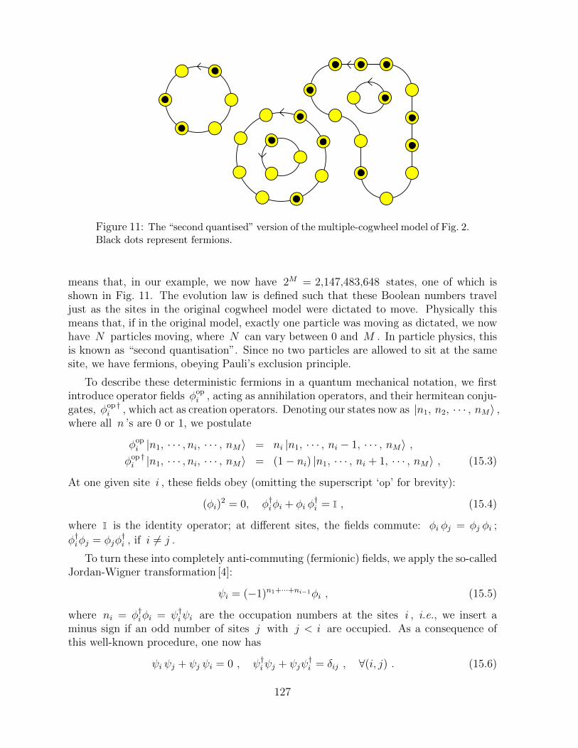
Figure 11: The “second quantised” version of the multiple-cogwheel model of Fig. 2.Black dots represent fermions.

means that, in our example, we now have 2M = 2,147,483,648 states, one of which isshown in Fig. 11. The evolution law is defined such that these Boolean numbers traveljust as the sites in the original cogwheel model were dictated to move. Physically thismeans that, if in the original model, exactly one particle was moving as dictated, we nowhave N particles moving, where N can vary between 0 and M . In particle physics, thisis known as “second quantisation”. Since no two particles are allowed to sit at the samesite, we have fermions, obeying Pauli’s exclusion principle.

To describe these deterministic fermions in a quantum mechanical notation, we firstintroduce operator fields φop

i , acting as annihilation operators, and their hermitean conju-gates, φop †

i , which act as creation operators. Denoting our states now as |n1, n2, · · · , nM〉 ,where all n ’s are 0 or 1, we postulate

φopi |n1, · · · , ni, · · · , nM〉 = ni |n1, · · · , ni − 1, · · · , nM〉 ,

φop †i |n1, · · · , ni, · · · , nM〉 = (1− ni) |n1, · · · , ni + 1, · · · , nM〉 , (15.3)

At one given site i , these fields obey (omitting the superscript ‘op’ for brevity):

(φi)2 = 0, φ†iφi + φi φ

†i = I , (15.4)

where I is the identity operator; at different sites, the fields commute: φi φj = φj φi ;

φ†iφj = φjφ†i , if i 6= j .

To turn these into completely anti-commuting (fermionic) fields, we apply the so-calledJordan-Wigner transformation [4]:

ψi = (−1)n1+···+ni−1φi , (15.5)

where ni = φ†iφi = ψ†iψi are the occupation numbers at the sites i , i.e., we insert aminus sign if an odd number of sites j with j < i are occupied. As a consequence ofthis well-known procedure, one now has

ψi ψj + ψj ψi = 0 , ψ†iψj + ψjψ†i = δij , ∀(i, j) . (15.6)

127

The virtue of this transformation is that the anti-commutation relations (15.6) stayunchanged after any linear, unitary transformation of the ψi as vectors in our M -dimensional vector space, provided that ψ†i transform as contra-vectors. Usually, theminus signs in Eq. (15.5) do no harm, but some care is asked for.

Now consider the permutation matrix P and write the Hamiltonian in Eq. (15.2) asa lower case hij ; it is an M ×M component matrix. Writing Uij(t) = (e−iht)ij , we have,at integer time steps, P t

op = Uop(t) . We now claim that the permutation that moves thefermions around, is generated by the Hamiltonian Hop

F defined as

HopF =

∑ij

ψ†j hji ψi . (15.7)

This we prove as follows:Let

ψi(t) = eiHopF t ψi e

−iHopF t ,

ddte−iH

opF t = −iHop

F e−iHopF t = −i e−iH

opF tHop

F ; (15.8)

Then

d

dtψk(t) = i eiH

opF t∑ij

[ψ†j hji ψi, ψk]e−iHop

F t = (15.9)

i eiHopF t∑ij

hji

(− ψ†j , ψkψi + ψ†jψi, ψk

)e−iH

opF t = (15.10)

− i eiHopF t∑i

hkiψi e−iHop

F t = − i∑i

hkiψi(t) , (15.11)

where the anti-commutator is defined as A, B ≡ AB+BA (note that the second termin Eq. (15.10) vanishes).

This is the same equation that describes the evolution of the states |k〉 of the originalcogwheel model. So we see that, at integer time steps t , the fields ψi(t) are permutedaccording to the permutation operator P t . Note now, that the empty state |0〉 (whichis not the vacuum state) does not evolve at all (and neither does the completely filledstate). The N particle state ( 0 ≤ N ≤M ), obtained by applying N copies of the fieldoperators ψ†i , therefore evolves with the same permutator. The Jordan Wigner minussign, (15.5), gives the transformed state a minus sign if after t permutations the orderof the N particles has become an odd permutation of their original relative positions.Although we have to be aware of the existence of this minus sign, it plays no significantrole in most cases. Physically, this sign is not observable.

The importance of the procedure displayed here is that we can read off how anti-commuting fermionic field operators ψi , or ψi(x) , can emerge from deterministic systems.The minus signs in their (anti-)commutators is due to the Jordan-Wigner transformation(15.5), without which we would not have any commutator expressions at all, so that thederivation (15.11) would have failed.

128

The final step in this second quantisation procedure is that we now use our freedomto perform orthogonal transformations among the fields ψ and ψ† , such that we expandthem in terms of the eigenstates ψ(Ei) of the one-particle Hamiltonian hij . Then thestate |∅〉 obeying

ψ(Ei)|∅〉 = 0 if Ei > 0 ; ψ†(Ei)|∅〉 = 0 if Ei < 0 , (15.12)

has the lowest energy of all. Now, that is the vacuum state, as Dirac proposed. Thenegative energy states are interpreted as holes for antiparticles. The operators ψ(E)annihilate particles if E > 0 or create antiparticles if E < 0 . For ψ†(E) it is theother way around. Particles and antiparticles now all carry positive energy. Is this thenthe resolution of the problem noted in chapter 14? This depends on how we handleinteractions, see chapter 9.2 in part I, and we discuss this important question further insection 22.1 and in chapter 23.

The conclusion of this section is that, if the Hamiltonian matrix hij describes asingle or composite cogwheel model, leading to classical permutations of the states |i〉 ,i = 1, · · · ,M , at integer times, then the model with Hamiltonian (15.7) is related to asystem where occupied states evolve according to the same permutations, the differencebeing that now the total number of states is 2M instead of M . And the energy is alwaysbounded from below.

One might object that in most physical systems the Hamiltonian matrix hij wouldnot lead to classical permutations at integer time steps, but our model is just a first step.A next step could be that hij is made to depend on the values of some local operatorfields ϕ(x) . This is what we have in the physical world, and this may result if thepermutation rules for the evolution of these fermionic particles are assumed to depend onother variables in the system.

In fact, there does exist a fairly realistic, simplified fermionic model where hij doesappear to generate pure permutations. This will be exhibited in the next section.

A procedure for bosons should go in analogous ways, if one deals with bosonic fields inquantum field theory. However, a relation with deterministic theories is not as straight-forward as in the fermionic case, because arbitrarily large numbers of bosonic particlesmay occupy a single site. To mitigate this situation, the notion of harmonic rotators wasintroduced, which also for bosons only allows finite numbers of states. We can applymore conventional bosonic second quantisation in some special two-dimensional theories,see subsection 17.1.1.

How second quantisation is applied in standard quantum field theories is described insection 20.3.

15.2. ‘Neutrinos’ in three space dimensions

In some cases, it is worth-while to start at the other end. Given a typical quantum system,can one devise a deterministic classical automaton that would generate all its quantumstates? We now show a new case of interest.

129

One way to determine whether a quantum system may be mathematically equivalentto a deterministic model is to search for a complete set of beables. As defined in subsec-tion 2.1.1, beables are operators that may describe classical observables, and as such theymust commute with one another, always, at all times. Thus, for conventional quantumparticles such as the electron in Bohr’s hydrogen model, neither the operators x nor pare beables because [ x(t) , x(t′) ] 6= 0 and [ p(t), p(t′) ] 6= 0 as soon as t 6= t′ . Typicalmodels where we do have such beables are ones where the Hamiltonian is linear in themomenta, such as in section 12.3, Eq. (12.18), rather than quadratic in p . But are theythe only ones?

Maybe the beables only form a space-time grid, whereas the data on points in betweenthe points on the grid do not commute. This would actually serve our purpose well, sinceit could be that the physical data characterising our universe really do form such a grid,while we have not yet been able to observe that, just because the grid is too fine for today’stools, and interpolations to include points in between the grid points could merely havebeen consequences of our ignorance.

Beables form a complete set if, in the basis where they are all diagonal, the collectionof eigenvalues completely identify the elements of this basis.

No such systems of beables do occur in nature, as far as we know today; that is, ifwe take all known forces into account, all operators that we can construct today ceaseto commute at some point. We can, and should, try to search better, but, alternatively,we can produce simplified models describing only parts of what we see, which do allowtransformations to a basis of beables. In chapter 12.1, we already discussed the harmonicrotator as an important example, which allowed for some interesting mathematics inchapter 13. Eventually, its large N limit should reproduce the conventional harmonicoscillator. Here, we discuss another such model: massless ‘neutrinos’, in 3 space-like andone time-like dimension.

A single quantised, non interacting Dirac fermion obeys the Hamiltonian34

Hop = αipi + βm , (15.13)

where αi, β are Dirac 4× 4 matrices obeying

αiαj + αjαi = 2δij ; β2 = 1 ; αi β + β αi = 0 . (15.14)

Only in the case m = 0 can we construct a complete set of beables, in a straightforwardmanner35. In that case, we can omit the matrix β , and replace αi by the three Paulimatrices, the 2 × 2 matrices σi . The particle can then be looked upon as a massless(Majorana or chiral) “neutrino”, having only two components in its spinor wave function.The neutrino is entirely ‘sterile’, as we ignore any of its interactions. This is why we callthis the ‘neutrino’ model, with ‘neutrino’ between quotation marks.

34Summation convention: repeated indices are usually summed over.35Massive ‘neutrinos’ could be looked upon as massless ones in a space with one or more extra dimen-

sions, and that does also have a beable basis. Projecting this set back to 4 space-time dimensions howeverleads to a rather contrived construction.

130

There are actually two choices here: the relative signs of the Pauli matrices could bechosen such that the particles have positive (left handed) helicity and the antiparticles areright handed, or they could be the other way around. We take the choice that particleshave the right handed helicities, if our coordinate frame (x, y, z) is oriented as the fingers1,2,3 of the right hand. The Pauli matrices σi obey

σ1 σ2 = iσ3 , σ2 σ3 = iσ1 , σ3 σ1 = iσ2 ; σ21 = σ2

2 = σ23 = 1 . (15.15)

The beables are:

Oopi = q, s, r , where

qi ≡ ±pi/|p| , s ≡ q · ~σ , r ≡ 12(q · ~x+ ~x · q) . (15.16)

To be precise, q is a unit vector defining the direction of the momentum, modulo its sign.What this means is that we write the momentum ~p as

~p = pr q , (15.17)

where pr can be a positive or negative real number. This is important, because we needits canonical commutation relation with the variable r , being [ r, pr ] = i , without furtherrestrictions on r or pr . If pr would be limited to the positive numbers |p| , this wouldimply analyticity constraints for wave functions ψ(r) .

The caret ˆ on the operator q is there to remind us that it is a vector with length one,|q| = 1 . To define its sign, one could use a condition such as qz > 0 . Alternatively, wemay decide to keep the symmetry Pint (for ‘internal parity’),

q ↔ −q , pr ↔ −pr , r ↔ −r , s↔ −s , (15.18)

after which we would keep only the wave functions that are even under this reflection.The variable s can only take the values s = ±1 , as one can check by taking the squareof q · ~σ . In the sequel, the symbol p will be reserved for p = +~p/|p| , so that q = ±p .

The last operator in Eq. (15.16), the operator r , was symmetrised so as to guaranteethat it is hermitean. It can be simplified by using the following observations. In the ~pbasis, we have

~x = i∂

∂~p;

∂

∂~ppr = q ; [xi, pr ] = iqi ; [xi, qj ] =

i

pr(δij − qiqj) ; (15.19)

xiqi − qixi =2i

pr→ 1

2(q · ~x+ ~x · q) = q · ~x+

i

pr. (15.20)

This can best be checked first by checking the case pr = |p| > 0, q = p , and noting thatall equations are preserved under the reflection symmetry (15.18).

It is easy to check that the operators (15.16) indeed form a completely commuting set.The only non-trivial commutator to be looked at carefully is [r, q] = [ q · ~x , q ] . Consider

131

again the ~p basis, where ~x = i∂/∂~p : the operator ~p · ∂/∂~p is the dilatation operator.But, since q is scale invariant, it commutes with the dilatation operator:

[ ~p · ∂∂~p

, q ] = 0 . (15.21)

Therefore,

[ q · ~x, q ] = i [ p−1r ~p · ∂

∂~p, q ] = 0 , (15.22)

since also [ pr, q ] = 0 , but of course we could also have used equation (15.19), # 4.

The unit vector q lives on a sphere, characterised by two angles θ and ϕ . If wedecide to define q such that qz > 0 then the domains in which these angles must lie are:

0 ≤ θ ≤ π/2 , 0 ≤ ϕ < 2π . (15.23)

The other variables take the values

s = ±1 , −∞ < r <∞ . (15.24)

An important question concerns the completeness of these beables and their relationto the more usual operates ~x, ~p and ~σ , which of course do not commute so that thesethemselves are no beables. This we discuss in the next subsection, which can be skipped atfirst reading. For now, we mention the more fundamental observation that these beablescan describe ontological observables at all times, since the Hamiltonian (15.13), whichhere reduces to

H = ~σ · ~p , (15.25)

generates the equations of motion

d

dt~x = −i[~x, H] = ~σ ,

d

dt~p = 0 ,

d

dtσi = 2εijk pj σk ; (15.26)

d

dtp = 0 ;

d

dt(p · ~σ) = 2εijk (pi/|p|) pjσk = 0 ,

d

dt(p · ~x) = p · ~σ , (15.27)

where p = ~p/|p| = ±q , and thus we have:

d

dtθ = 0 ,

d

dtϕ = 0 ,

d

dts = 0 ,

d

dtr = s = ± 1 . (15.28)

The physical interpretation is simple: the variable r is the position of a ‘particle’projected along a predetermined direction q , given by the two angles θ and ϕ , and thesign of s determines whether it moves with the speed of light towards larger or towardssmaller r values.

132

Note, that a rotation over 180 along an axis orthogonal to q may turn s into −s ,which is characteristic for half-odd spin representations of the rotation group, so that wecan still consider the neutrino as a spin 1

2particle.36

What we have here is a representation of the wave function for a single ‘neutrino’ inan unusual basis. As will be clear from the calculations presented in the subsection below,in this basis the ‘neutrino’ is entirely non localised in the two transverse directions, butits direction of motion is entirely fixed by the unit vector q and the Boolean variable s .In terms of this basis, the ‘neutrino’ is a deterministic object. Rather than saying thatwe have a particle here, we have a flat sheet, a plane. The unit vector q describes theorientation of the plane, and the variable s tells us in which of the two possible directionsthe plane moves, always with the speed of light. Neutrinos are deterministic planes, orflat sheets. The basis in which the operators q, r , and s are diagonal will serve as anontological basis.

Finally, we could use the Boolean variable s to define the sign of q , so that it becomesa more familiar unit vector, but this can better be done after we studied the operatorsthat flip the sign of the variable s , because of a slight complication, which is discussedwhen we work out the algebra, in subsections 15.2.1 and 15.2.2.

Clearly, operators that flip the sign of s exist. For that, we take any vector q ′ thatis orthogonal to q . Then, the operator q ′ · ~σ obeys (q ′ · ~σ) s = −s (q ′ · ~σ) , as onecan easily check. So, this operator flips the sign. The problem is that, at each point onthe sphere of q values, one can take any unit length superposition of two such vectorsq ′ orthogonal to q . Which one should we take? Whatever our choice, it depends onthe angles θ and ϕ . This implies that we necessarily introduce some rather unpleasantangular dependence. This is inevitable; it is caused by the fact that the original neutrinohad spin 1

2, and we cannot mimic this behaviour in terms of the q dependence because

all wave functions have integral spin. One has to keep this in mind whenever the Paulimatrices are processed in our descriptions.

Thus, in order to complete our operator algebra in the basis determined by the eigen-values q, s, and r , we introduce two new operators whose squares ore one. Define twovectors orthogonal to q , one in the θ -direction and one in the ϕ -direction:

q =

q1

q2

q3

, θ =1√

q21 + q2

2

q3 q1

q3 q2

q23 − 1

, ϕ =1√

q21 + q2

2

−q2

q1

0

. (15.29)

All three are normalised to one, as indicated by the caret. Their components obey

qi = εijk θjϕk , θi = εijk ϕjqk , ϕi = εijk qjθk . (15.30)

Then we define two sign-flip operators: write s = s3 , then

s1 = θ · ~σ , s2 = ϕ · ~σ , s3 = s = q · ~σ . (15.31)

36But rotations in the plane, or equivalently, around the axis q , give rise to complications, which canbe overcome, see later in this section.

133

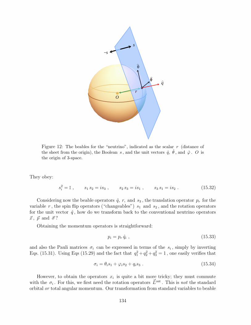
θ

ϕq

Or

s

−s

Figure 12: The beables for the “neutrino”, indicated as the scalar r (distance ofthe sheet from the origin), the Boolean s , and the unit vectors q, θ , and ϕ . O isthe origin of 3-space.

They obey:

s2i = I , s1 s2 = is3 , s2 s3 = is1 , s3 s1 = is2 . (15.32)

Considering now the beable operators q, r, and s3 , the translation operator pr for thevariable r , the spin flip operators (“changeables”) s1 and s2 , and the rotation operatorsfor the unit vector q , how do we transform back to the conventional neutrino operators~x , ~p and ~σ ?

Obtaining the momentum operators is straightforward:

pi = pr qi , (15.33)

and also the Pauli matrices σi can be expressed in terms of the si , simply by invertingEqs. (15.31). Using Eqs (15.29) and the fact that q2

1 + q22 + q2

3 = 1 , one easily verifies that

σi = θis1 + ϕis2 + qis3 . (15.34)

However, to obtain the operators xi is quite a bit more tricky; they must commutewith the σi . For this, we first need the rotation operators ~Lont . This is not the standardorbital or total angular momentum. Our transformation from standard variables to beable

134

variables will not be quite rotationally invariant, just because we will be using either theoperator s1 or the operator s2 to go from a left-moving neutrino to a right moving one.Note, that in the standard picture, chiral neutrinos have spin 1

2. So flipping from one

mode to the opposite one involves one unit ~ of angular momentum in the plane. Theontological basis does not refer to neutrino spin, and this is why our algebra gives somespurious angular momentum violation. As long as neutrinos do not interact, this effectstays practically unnoticeable, but care is needed when either interactions or mass areintroduced.

The only rotation operators we can start off with in the beable frame, are the operatorsthat rotate the planes with respect to the origin of our coordinates. These we call ~Lont :

Lonti = −iεijkqj

∂

∂qk. (15.35)

By definition, they commute with the si , but care must be taken at the equator, wherewe have a boundary condition, which can be best understood by imposing the symmetrycondition (15.18).

Note that the operators Lonti defined in Eq. (15.35) do not coincide with any of the

conventional angular momentum operators because those do not commute with the si ,as the latter depend on θ and ϕ . One finds the following relation between the angularmomentum ~L of the neutrinos and ~L ont :

Lonti ≡ Li + 1

2

(θis1 + ϕis2 −

q3 θi√1− q2

3

s3

); (15.36)

the derivation of this equation is postponed to subsection 15.2.1.

Since ~J = ~L+ 12~σ , one can also write, using Eqs. (15.34) and (15.29),

Lonti = Ji −

1

1− q23

q1

q2

0

s3 . (15.37)

We then derive, in subsection 15.2.1, Eq. (15.60), the following expression for theoperators xi in the neutrino wave function, in terms of the beables q, r and s3 , and thechangeables37 Lont

k , pr , s1 and s2 :

xi = qi (r −i

pr) + εijk qj L

ontk /pr +

1

2pr

(−ϕi s1 + θi s2 +

q3√1− q2

3

ϕi s3

)(15.38)

(note that θi and ϕi are beables since they are functions of q ).

The complete transformation from the beable basis to one of the conventional basesfor the neutrino can be derived from

〈~p, α | q, pr, s〉 = pr δ3(~p− q pr)χsα(q) , (15.39)

37See Eq. (15.47) and the remarks made there concerning the definition of the operator 1/pr in theworld of the beables, as well as in the end of section 15.2.2.

135

where α is the spin index of the wave functions in the basis where σ3 is diagonal, andχsα is a standard spinor solution for the equation (q · ~σαβ)χsβ(q) = s χsα(q) .

In subsection 15.2.2, we show how this equation can be used to derive the elements ofthe unitary transformation matrix mapping the beable basis to the standard coordinateframe of the neutrino wave function basis38 (See Eq. 15.83):

〈 ~x, α | q, r, s 〉 =i

2πδ ′(r − q · ~x )χsα(q) , (15.40)

where δ ′(z) ≡ ddzδ(z) . This derivative originates from the factor pr in Eq. (15.39), which

is necessary for a proper normalisation of the states.

15.2.1. Algebra of the beable ‘neutrino’ operators

This subsection is fairly technical and can be skipped at first reading. It derives the resultsmentioned in the previous section, by handling the algebra needed for the transformationsfrom the (q, s, r) basis to the (~x, σ3) or (~p, σ3) basis and back. This algebra is fairlycomplex, again, because, in the beable representation, no direct reference is made toneutrino spin. Chiral neutrinos are normally equipped with spin +1

2or −1

2with spin

axis in the direction of motion. The flat planes that are moving along here, are invariantunder rotations about an orthogonal axis, and the associated spin-angular momentumdoes not leave a trace in the non-interacting, beable picture.

This forces us to introduce some axis inside each plane that defines the phases of thequantum states, and these (unobservable) phases explicitly break rotation invariance.

We consider the states specified by the variables s and r , and the polar coordinatesθ and ϕ of the beable q , in the domains given by Eqs. (15.23), (15.24). Thus, we havethe states |θ, ϕ, s, r〉 . How can these be expressed in the more familiar states |~x, σz〉and/or |~p, σz〉 , where σz = ±1 describes the neutrino spin in the z -direction, and viceversa?

Our ontological states are specified in the ontological basis spanned by the operatorsq, s (= s3), and r . We add the operators (changeables) s1 and s2 by specifying theiralgebra (15.32), and the operator

pr = −i∂/∂r ; [ r, pr] = i . (15.41)

The original momentum operators are then easily retrieved. As in Eq, (15.17), define

~p = pr q . (15.42)

The next operators that we can reproduce from the beable operators q, r , and s1,2,3

are the Pauli operators σ1,2,3 :

σi = θis1 + ϕis2 + qis3 . (15.43)

38In this expression, there is no need to symmetrise q ·~x , because both q and ~x consist of C-numbersonly.

136

Note, that these now depend non-trivially on the angular parameters θ and ϕ , since thevectors θ and ϕ , defined in Eq. (15.29), depend non-trivially on q , which is the radialvector specified by the angles θ and ϕ . One easily checks that the simple multiplicationrules from Eqs. (15.32) and the right-handed orthonormality (15.30) assure that thesePauli matrices obey the correct multiplication rules also. Given the trivial commutationrules for the beables, [qi, θj] = [qi, ϕj] = 0 , and [pr, qi] = 0 , one finds that [pi, σj] = 0 ,so here, we have no new complications.

Things are far more complicated and delicate for the ~x operators. To reconstructan operator ~x = i∂/∂~p , obeying [xi, pj] = iδij and [xi, σj] = 0 , we first introduce theorbital angular momentum operator

Li = εijkxipk = −iεijkqj∂

∂qk(15.44)

(where σi are kept fixed), obeying the usual commutation rules

[Li, Lj] = iεijkLk , [Li, qj] = iεijkqk , [Li, pj] = iεijkpk , etc., (15.45)

while [Li, σj] = 0 . Note, that these operators are not the same as the angular momentain the ontological frame, the Lont

i of Eq. (15.35), since those are demanded to commutewith sj , while the orbital angular momenta Li commute with σj . In terms of the orbitalangular momenta (15.44), we can now recover the original space operators xi, i = 1, 2, 3 ,of the neutrinos:

xi = qi (r −i

pr) + εijk qj Lk/pr . (15.46)

The operator 1/pr , the inverse of the operator pr = −i∂/∂r , should be −i times theintegration operator. This leaves the question of the integration constant. It is straight-forward to define that in momentum space, but eventually, r is our beable operator.For wave functions in r space, ψ(r, · · ·) = 〈r, · · · |ψ〉 , where the ellipses stand for otherbeables (of course commuting with r ), the most careful definition is:

1

prψ(r) ≡

∫ ∞−∞

12i sgn(r − r′)ψ(r′)dr′ , (15.47)

which can easily be seen to return ψ(r) when pr acts on it. “sgn(x )” stands for the signof x . We do note that the integral must converge at r → ±∞ . This is a restrictionon the class of allowed wave functions: in momentum space, ψ must vanish at pr → 0 .Restrictions of this sort will be encountered more frequently in this book.

The anti hermitean term −i/pr in Eq. (15.46) arises automatically in a careful cal-culation, and it just compensates the non hermiticity of the last term, where qj and Lkshould be symmetrised to get a hermitean expression. Lk commutes with pr . The xidefined here ends up being hermitean.

This perhaps did not look too hard, but we are not ready yet. The operators Licommute with σj , but not with the beable variables si . Therefore, an observer of the

137

beable states, in the beable basis, will find it difficult to identify our operators Li . It willbe easy for such an observer to identify operators Lont

i , which generate rotations of the qivariables while commuting with si . He might also want to rotate the Pauli-like variablessi , employing a rotation operator such as 1

2si , but that will not do, first, because they

no longer obviously relate to spin, but foremost, because the si in the conventional basishave a much less trivial dependence on the angles θ and ϕ , see Eqs. (15.29) and (15.31).

Actually, the reconstruction of the ~x operators from the beables will show a non-trivial dependence on the variables si and the angles θ and ϕ . This is because ~x andthe si do not commute. From the definitions (15.29) and the expressions (15.29) for thethe vectors θ and ϕ , one derives, from judicious calculations:

[xi, θj] =i

pr

( q3√1− q2

3

ϕi ϕj − θi qj), (15.48)

[xi, ϕj] =−iϕipr

(qj +

θj q3√1− q2

3

), (15.49)

[xi, qj] =i

pr(δij − qi qj) . (15.50)

The expression q3/√

1− q23 = cot(θ) emerging here is singular at the poles, clearly due

to the vortices there in the definitions of the angular directions θ and ϕ .

From these expressions, we now deduce the commutators of xi and s1,2,3 :

[xi, s1] =i

pr

( ϕi q3√1− q2

3

s2 − θi s3

), (15.51)

[xi, s2] =−iprϕi

(s3 +

q3√1− q2

3

s1

), (15.52)

[xi, s3] =i

pr(σi − qi s3) =

i

pr(θi s1 + ϕi s2) . (15.53)

In the last expression Eq. (15.43) for ~σ was used. Now, observe that these equations canbe written more compactly:

[xi, sj] = 12

[ 1

pr

(− ϕis1 + θis2 +

q3 ϕi√1− q2

3

s3

), sj

]. (15.54)

To proceed correctly, we now need also to know how the angular momentum operatorsLi commute with s1,2,3 . Write Li = εijkxj qk pr , where only the functions xi do notcommute with the sj . It is then easy to use Eqs. (15.51)—(15.54) to find the desiredcommutators:

[Li, sj] = 12

[− θis1 − ϕis2 +

q3 θi√1− q2

3

s3, sj

], (15.55)

where we used the simple orthonormality relations (15.30) for the unit vectors θ, ϕ , andq . Now, this means that we can find new operators Lont

i that commute with all the sj :

Lonti ≡ Li + 1

2

(θis1 + ϕis2 −

q3 θi√1− q2

3

s3

), [Lont

i , sj] = 0 , (15.56)

138

as was anticipated in Eq. 15.36. It is then of interest to check the commutator of two ofthe new “angular momentum” operators. One thing we know: according to the Jacobiidentity, the commutator of two operators Lont

i must also commute with all sj . Now,expression (15.56) seems to be the only one that is of the form expected, and commuteswith all s operators. It can therefore be anticipated that the commutator of two Lont

operators should again yield an Lont operator, because other expressions could not pos-sibly commute with all s . The explicit calculation of the commutator is a bit awkward.For instance, one must not forget that Li also commutes non-trivially with cot(θ) :

[Li,q3√

1− q23

] =iϕi

1− q23

. (15.57)

But then, indeed, one finds [Lonti , Lont

j

]= iεijkL

ontk . (15.58)

The commutation rules with qi and with r and pr were not affected by the additionalterms:

[Lonti , qj] = iεijk qk , [Lont

i , r] = [Lonti , pr] = 0 . (15.59)

This confirms that we now indeed have the generator for rotations of the beables qi , whileit does not affect the other beables si, r and pr .

Thus, to find the correct expression for the operators ~x in terms of the beable variables,we replace Li in Eq. (15.46) by Lont

i , leading to

xi = qi (r −i

pr) + εijk qj L

ontk /pr +

1

2pr

(−ϕi s1 + θi s2 +

q3√1− q2

3

ϕi s3

). (15.60)

This remarkable expression shows that, in terms of the beable variables, the ~x coordi-nates undergo finite, angle-dependent displacements proportional to our sign flip operatorss1, s2 , and s3 . These displacements are in the plane. However, the operator 1/pr doessomething else. From Eq. (15.47) we infer that, in the r variable,

〈r1|1

pr|r2〉 = 1

2i sgn(r1 − r2) . (15.61)

Returning now to a remark made earlier in this chapter, one might decide to use thesign operator s3 (or some combination of the three s variables) to distinguish oppositesigns of the q operators. The angles θ and ϕ then occupy the domains that are moreusual for an S2 sphere: 0 < θ < π , and 0 < ϕ ≤ 2π . In that case, the operators s1,2,3

refer to the signs of q3, r and pr . Not much would be gained by such a notation.

The Hamiltonian in the conventional basis is

H = ~σ · ~p . (15.62)

139

It is linear in the momenta pi , but it also depends on the non commuting Pauli matricesσi . This is why the conventional basis cannot be used directly to see that this is adeterministic model. Now, in our ontological basis, this becomes

H = s pr . (15.63)

Thus, it multiplies one momentum variable with the commuting operator s . The Hamil-ton equation reads

dr

dt= s , (15.64)

while all other beables stay constant. This is how our ‘neutrino’ model became determin-istic. In the basis of states | q, r, s 〉 our model clearly describes planar sheets at distancer from the origin, oriented in the direction of the unit vector q , moving with the velocityof light in a transverse direction, given by the sign of s .

Once we defined, in the basis of the two eigenvalues of s , the two other operators s1

and s2 , with (see Eqs. (15.32))

s1 =

(0 11 0

), s2 =

(0 −ii 0

), s3 = s =

(1 00 −1

), (15.65)

in the basis of states | r 〉 the operator pr = −i∂/∂r , and, in the basis | q 〉 the operatorsLonti by

[Lonti , Lont

j ] = iεijkLontk , [Lont

i , qj] = iεijk qk , [Lonti , r] = 0 , [Lont

i , sj] = 0 , (15.66)

we can write, in the ‘ontological’ basis, the conventional ‘neutrino’ operators ~σ (Eq.(15.43)), ~x (Eq. (15.60)), and ~p (Eq. (15.42)). By construction, these will obey thecorrect commutation relations.

15.2.2. Orthonormality and transformations of the ‘neutrino’ beable states

The quantities that we now wish to determine are the inner products

〈~x, σz|θ, ϕ, s, r〉 , 〈~p, σz|θ, ϕ, s, r〉 . (15.67)

The states | θ, ϕ, s, r〉 will henceforth be written as | q, s, r〉 . The use of momentumvariables q ≡ ±~p/|p| , qz > 0, together with a real parameter r inside a Dirac bracketwill always denote a beable state in this subsection.

Special attention is required for the proper normalisation of the various sets of eigen-states. We assume the following normalisations:

〈~x, α | ~x ′, β〉 = δ3(~x− ~x ′) δαβ , (15.68)

〈~p, α | ~p ′, β〉 = δ3(~p− ~p ′) δαβ , (15.69)

〈~x, α | ~p, β〉 = (2π)−3/2 ei ~p·~x δαβ ; (15.70)

〈q, r, s | q ′, r′, s′ 〉 = δ2(q, q ′) δ(r − r′) δs s′ , (15.71)

δ2(q, q′) ≡ δ(θ − θ′) δ(ϕ− ϕ′)sin θ

, (15.72)

140

and α and β are eigenvalues of the Pauli matrix σ3 ; furthermore,∫δ3~x

∑α

| ~x, α〉〈~x, α | = I =

∫d2q

∫ ∞−∞

dr∑s=±

| q, r, s〉〈q, r, s | ;

∫d2q ≡

∫ π/2

0

sin θ dθ

∫ 2π

0

dϕ . (15.73)

The various matrix elements are now straightforward to compute. First we define thespinors χ±α (q) by solving

(q · ~σαβ)χsβ = s χsα ;

(q3 − s q1 − iq2

q1 + iq2 −q3 − s

)(χs1χs2

)= 0 , (15.74)

which gives, after normalising the spinors,

χ+1 (q) =

√12(1 + q3)

χ+2 (q) =

q1 + i q2√2(1 + q3)

;

χ−1 (q) = −√

12(1− q3)

χ−2 (q) =q1 + i q2√2(1− q3)

, (15.75)

where not only the equation s3 χ±α = ±χ±α was imposed, but also

s α1β χ

±α = χ∓β , s α

2β χ±α = ± i χ∓β , (15.76)

which implies a constraint on the relative phases of χ+α and χ−α . The sign in the second of

these equations is understood if we realise that the index s here, and later in Eq. (15.80),is an upper index.

Next, we need to know how the various Dirac deltas are normalised:

d3~p = p2r d2q dpr ; δ3(q pr − q ′ pr′) =

1

p2r

δ2(q, q ′) δ(pr − pr′) , (15.77)

We demand completeness to mean∫d2q

∫ ∞−∞

dpr∑s=±

〈 ~p, α | q, pr, s 〉〈 q, pr, s | ~p ′, α′〉 = δαα′δ3(~p− ~p ′) ; (15.78)

∫d3~p

2∑α=1

〈 q, pr, s | ~p, α 〉〈 ~p, α | q ′, pr′, s′ 〉 = δ2(q, q ′)δ(pr − pr′) δss′ , (15.79)

which can easily be seen to imply39

〈~p, α | q, pr, s〉 = pr δ3(~p− q pr)χsα(q) , (15.80)

since the norm p2r has to be divided over the two matrix terms in Eqs (15.78) and (15.79).

39Note that the phases in these matrix elements could be defined at will, so we could have chosen |p|in stead of pr . Our present choice is for future convenience.

141

This brings us to derive, using 〈 r | pr 〉 = (2π)−1/2 e i pr r ,

〈 ~p, α | q, r, s 〉 =1√2π

1

prδ2(±~p|p|

, q)e−i(q · ~p ) r χsα(q) , (15.81)

where the sign is the sign of p3 .

The Dirac delta in here can also be denoted as

δ2(±~p|p|

, q)

= (q · ~p )2 δ2(~p ∧ q) , (15.82)

where the first term is a normalisation to ensure the expression to become scale invariant,and the second just forces ~p and q to be parallel or antiparallel. In the case q = (0, 0, 1) ,this simply describes p2

3 δ(p1) δ(p2) .

Finally then, we can derive the matrix elements 〈 ~x, α | q, r, s 〉 . Just temporarily, weput q in the 3-direction: q = (0, 0, 1) ,

〈 ~x, α | q, r, s 〉 =1√2π

(2π)−3/2

∫d3~p

(q · ~p )2

prδ2(~p ∧ q)e−i(q · ~p ) r + i ~p · ~x χsα(q) =

=1

(2π)2

∫d3~p p3 δ(p1) δ(p2) ei p3(x3 − r) χsα(q) =

=1

2π

id

drδ(r − q · ~x )χsα(q) =

i

2πδ ′(r − q · ~x )χsα(q) . (15.83)

With these equations, our transformation laws are now complete. We have all matrixelements to show how to go from one basis to another. Note, that the states with vanishingpr , the momentum of the sheets, generate singularities. Thus, we see that the states |ψ 〉with 〈pr = 0 |ψ 〉 6= 0 , or equivalently, 〈 ~p = 0 |ψ 〉 6= 0 , must be excluded. We call suchstates ‘edge states’, since they have wave functions that are constant in space (in r andalso in ~x ), which means that they stretch to the ‘edge’ of the universe. There is an issuehere concerning the boundary conditions at infinity, which we will need to avoid. We seethat the operator 1/pr , Eq. (15.47), is ill defined for these states.

15.2.3. Second quantisation of the ‘neutrinos’

Being a relativistic Dirac fermion, the object described in this chapter so-far suffers fromthe problem that its Hamiltonian, (15.25) and (15.63), is not bounded from below. Thereare positive and negative energy states. The cure will be the same as the one used byDirac, and we will use it again later: second quantisation. We follow the proceduredescribed in section 15.1: for every given value of the unit vector q , we consider anunlimited number of ‘neutrinos’, which can be in positive or negative energy states. Tobe more specific, one might, temporarily, put the variables r on a discrete lattice:

r = rn = n δr , (15.84)

but often we ignore this, or in other words, we let δr tend to zero.

142

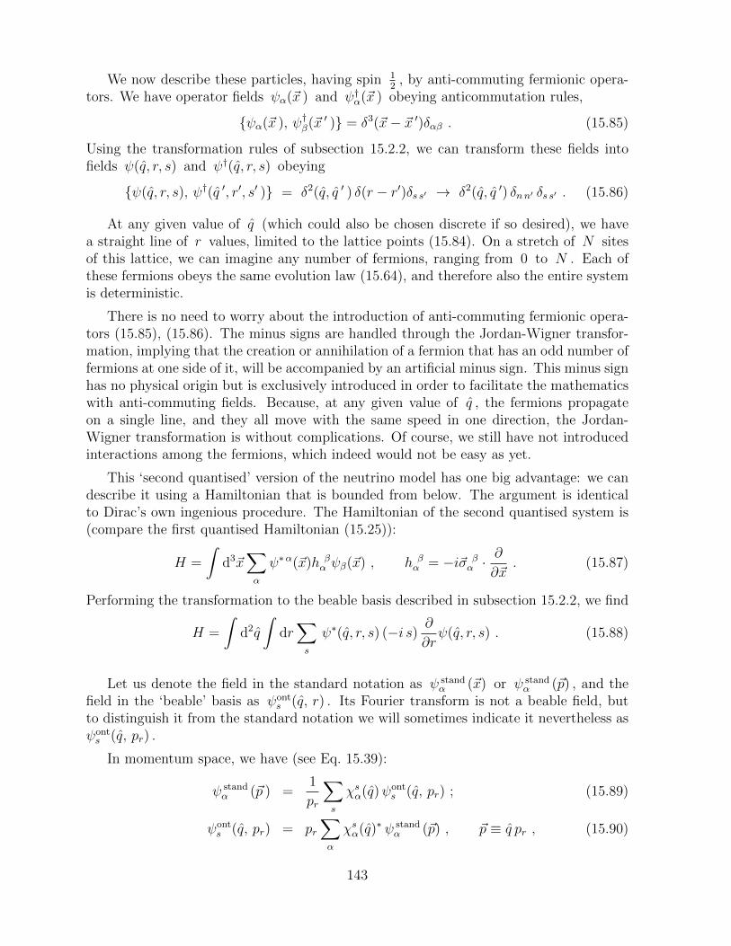
We now describe these particles, having spin 12

, by anti-commuting fermionic opera-tors. We have operator fields ψα(~x ) and ψ†α(~x ) obeying anticommutation rules,

ψα(~x ), ψ†β(~x ′ ) = δ3(~x− ~x ′)δαβ . (15.85)

Using the transformation rules of subsection 15.2.2, we can transform these fields intofields ψ(q, r, s) and ψ†(q, r, s) obeying

ψ(q, r, s), ψ†(q ′, r′, s′ ) = δ2(q, q ′ ) δ(r − r′)δs s′ → δ2(q, q ′) δnn′ δs s′ . (15.86)

At any given value of q (which could also be chosen discrete if so desired), we havea straight line of r values, limited to the lattice points (15.84). On a stretch of N sitesof this lattice, we can imagine any number of fermions, ranging from 0 to N . Each ofthese fermions obeys the same evolution law (15.64), and therefore also the entire systemis deterministic.

There is no need to worry about the introduction of anti-commuting fermionic opera-tors (15.85), (15.86). The minus signs are handled through the Jordan-Wigner transfor-mation, implying that the creation or annihilation of a fermion that has an odd number offermions at one side of it, will be accompanied by an artificial minus sign. This minus signhas no physical origin but is exclusively introduced in order to facilitate the mathematicswith anti-commuting fields. Because, at any given value of q , the fermions propagateon a single line, and they all move with the same speed in one direction, the Jordan-Wigner transformation is without complications. Of course, we still have not introducedinteractions among the fermions, which indeed would not be easy as yet.

This ‘second quantised’ version of the neutrino model has one big advantage: we candescribe it using a Hamiltonian that is bounded from below. The argument is identicalto Dirac’s own ingenious procedure. The Hamiltonian of the second quantised system is(compare the first quantised Hamiltonian (15.25)):

H =

∫d3~x

∑α

ψ∗α(~x)h βα ψβ(~x) , h β

α = −i~σ βα ·

∂

∂~x. (15.87)

Performing the transformation to the beable basis described in subsection 15.2.2, we find

H =

∫d2q

∫dr∑s

ψ∗(q, r, s) (−i s) ∂

∂rψ(q, r, s) . (15.88)

Let us denote the field in the standard notation as ψ standα (~x) or ψ stand

α (~p) , and thefield in the ‘beable’ basis as ψont

s (q, r) . Its Fourier transform is not a beable field, butto distinguish it from the standard notation we will sometimes indicate it nevertheless asψonts (q, pr) .

In momentum space, we have (see Eq. 15.39):

ψ standα (~p ) =

1

pr

∑s

χsα(q)ψonts (q, pr) ; (15.89)

ψonts (q, pr) = pr

∑α

χsα(q)∗ ψ standα (~p) , ~p ≡ q pr , (15.90)

143

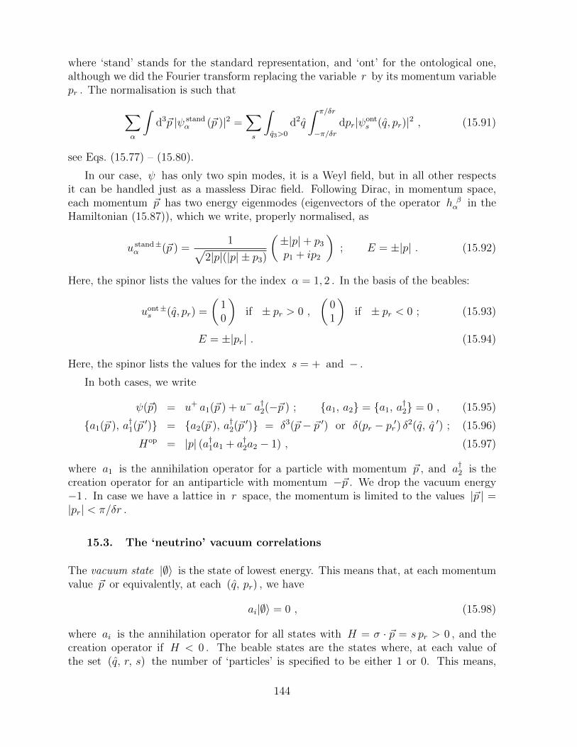
where ‘stand’ stands for the standard representation, and ‘ont’ for the ontological one,although we did the Fourier transform replacing the variable r by its momentum variablepr . The normalisation is such that

∑α

∫d3~p |ψ stand

α (~p )|2 =∑s

∫q3>0

d2q

∫ π/δr

−π/δrdpr|ψont

s (q, pr)|2 , (15.91)

see Eqs. (15.77) – (15.80).

In our case, ψ has only two spin modes, it is a Weyl field, but in all other respectsit can be handled just as a massless Dirac field. Following Dirac, in momentum space,each momentum ~p has two energy eigenmodes (eigenvectors of the operator h β

α in theHamiltonian (15.87)), which we write, properly normalised, as

u stand±α (~p ) =

1√2|p|(|p| ± p3)

(±|p|+ p3

p1 + ip2

); E = ±|p| . (15.92)

Here, the spinor lists the values for the index α = 1, 2 . In the basis of the beables:

uont±s (q, pr) =

(10

)if ± pr > 0 ,

(01

)if ± pr < 0 ; (15.93)

E = ±|pr| . (15.94)

Here, the spinor lists the values for the index s = + and − .

In both cases, we write

ψ(~p) = u+ a1(~p ) + u− a†2(−~p ) ; a1, a2 = a1, a†2 = 0 , (15.95)

a1(~p ), a†1(~p ′) = a2(~p ), a†2(~p ′) = δ3(~p− ~p ′) or δ(pr − pr′) δ2(q, q ′) ; (15.96)

Hop = |p| (a†1a1 + a†2a2 − 1) , (15.97)

where a1 is the annihilation operator for a particle with momentum ~p , and a†2 is thecreation operator for an antiparticle with momentum −~p . We drop the vacuum energy−1 . In case we have a lattice in r space, the momentum is limited to the values |~p | =|pr| < π/δr .

15.3. The ‘neutrino’ vacuum correlations

The vacuum state |∅〉 is the state of lowest energy. This means that, at each momentumvalue ~p or equivalently, at each (q, pr) , we have

ai|∅〉 = 0 , (15.98)

where ai is the annihilation operator for all states with H = σ · ~p = s pr > 0 , and thecreation operator if H < 0 . The beable states are the states where, at each value ofthe set (q, r, s) the number of ‘particles’ is specified to be either 1 or 0. This means,

144

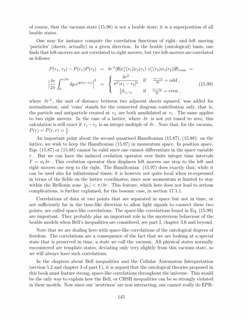
of course, that the vacuum state (15.98) is not a beable state; it is a superposition of allbeable states.

One may for instance compute the correlation functions of right- and left moving‘particles’ (sheets, actually) in a given direction. In the beable (ontological) basis, onefinds that left-movers are not correlated to right movers, but two left-movers are correlatedas follows:

P (r1, r2)− P (r1)P (r2) = δr 2〈∅|ψ∗s(r1)ψs(r1) ψ∗s(r2)ψs(r2)|∅〉conn =

∣∣∣ δr2π

∫ π/δr

0

dp eip(r2−r1)∣∣∣2 =

δr2

π2 |r1 − r2|2if r1−r2

δr= odd ,

14δr1, r2 if r1−r2

δr= even ,

(15.99)

where δr 2 , the unit of distance between two adjacent sheets squared, was added fornormalisation, and ‘conn’ stands for the connected diagram contribution only, that is,the particle and antiparticle created at r2 are both annihilated at r1 . The same appliesto two right movers. In the case of a lattice, where δr is not yet tuned to zero, thiscalculation is still exact if r1−r2 is an integer multiple of δr . Note that, for the vacuum,P (r) = P (r, r) = 1

2.

An important point about the second quantised Hamiltonian (15.87), (15.88): on thelattice, we wish to keep the Hamiltonian (15.97) in momentum space. In position space,Eqs. (15.87) or (15.88) cannot be valid since one cannot differentiate in the space variabler . But we can have the induced evolution operator over finite integer time intervalsT = nt δr . This evolution operator then displaces left movers one step to the left andright movers one step to the right. The Hamiltonian (15.97) does exactly that, while itcan be used also for infinitesimal times; it is however not quite local when re-expressedin terms of the fields on the lattice coordinates, since now momentum is limited to staywithin the Brillouin zone |pr| < π/δr . This feature, which here does not lead to seriouscomplications, is further explained, for the bosonic case, in section 17.1.1.

Correlations of data at two points that are separated in space but not in time, ornot sufficiently far in the time-like direction to allow light signals to connect these twopoints, are called space-like correlations. The space-like correlations found in Eq. (15.99)are important. They probably play an important role in the mysterious behaviour of thebeable models when Bell’s inequalities are considered, see part I, chapter 3.6 and beyond.

Note that we are dealing here with space-like correlations of the ontological degrees offreedom. The correlations are a consequence of the fact that we are looking at a specialstate that is preserved in time, a state we call the vacuum. All physical states normallyencountered are template states, deviating only very slightly from this vacuum state, sowe will always have such correlations.

In the chapters about Bell inequalities and the Cellular Automaton Interpretation(section 5.2 and chapter 3 of part I ), it is argued that the ontological theories proposed inthis book must feature strong, space-like correlations throughout the universe. This wouldbe the only way to explain how the Bell, or CHSH inequalities can be so strongly violatedin these models. Now since our ‘neutrinos’ are non interacting, one cannot really do EPR-

145

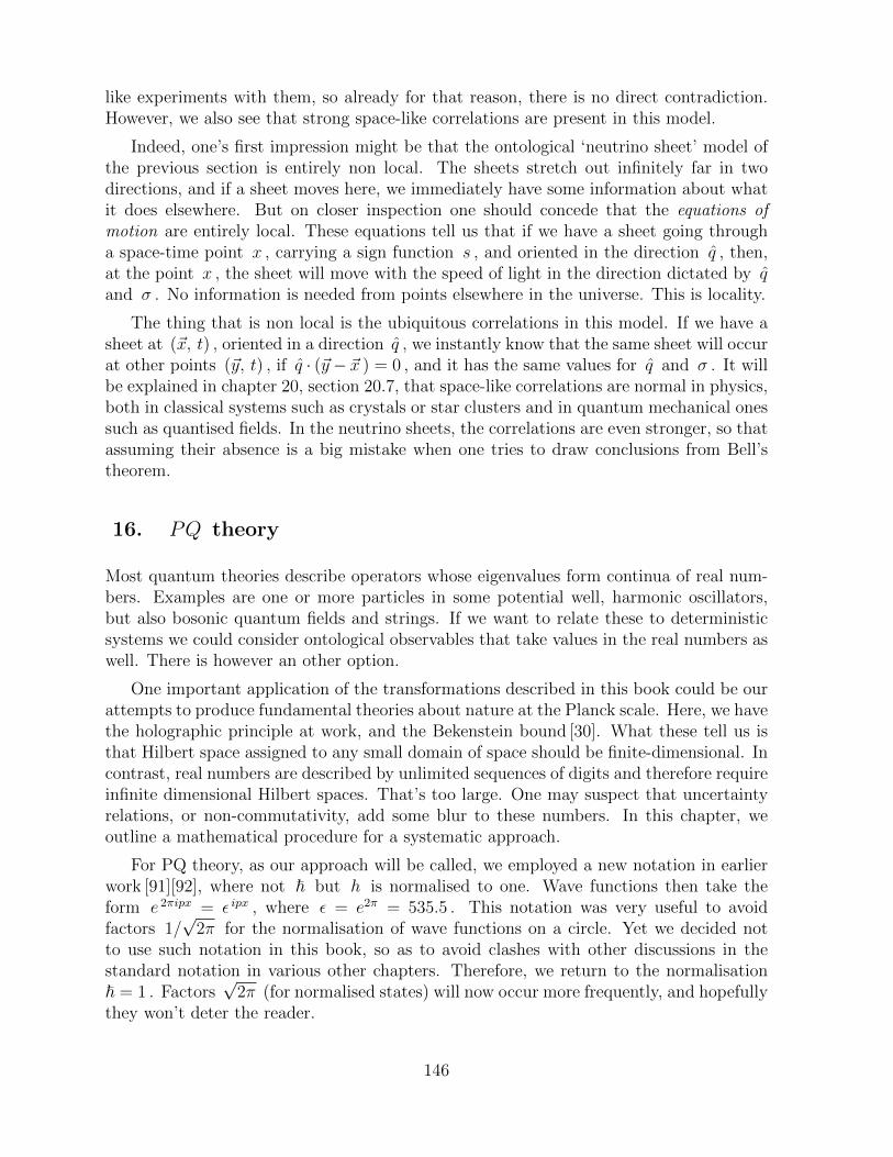
like experiments with them, so already for that reason, there is no direct contradiction.However, we also see that strong space-like correlations are present in this model.

Indeed, one’s first impression might be that the ontological ‘neutrino sheet’ model ofthe previous section is entirely non local. The sheets stretch out infinitely far in twodirections, and if a sheet moves here, we immediately have some information about whatit does elsewhere. But on closer inspection one should concede that the equations ofmotion are entirely local. These equations tell us that if we have a sheet going througha space-time point x , carrying a sign function s , and oriented in the direction q , then,at the point x , the sheet will move with the speed of light in the direction dictated by qand σ . No information is needed from points elsewhere in the universe. This is locality.

The thing that is non local is the ubiquitous correlations in this model. If we have asheet at (~x, t) , oriented in a direction q , we instantly know that the same sheet will occurat other points (~y, t) , if q · (~y− ~x ) = 0 , and it has the same values for q and σ . It willbe explained in chapter 20, section 20.7, that space-like correlations are normal in physics,both in classical systems such as crystals or star clusters and in quantum mechanical onessuch as quantised fields. In the neutrino sheets, the correlations are even stronger, so thatassuming their absence is a big mistake when one tries to draw conclusions from Bell’stheorem.

16. PQ theory

Most quantum theories describe operators whose eigenvalues form continua of real num-bers. Examples are one or more particles in some potential well, harmonic oscillators,but also bosonic quantum fields and strings. If we want to relate these to deterministicsystems we could consider ontological observables that take values in the real numbers aswell. There is however an other option.

One important application of the transformations described in this book could be ourattempts to produce fundamental theories about nature at the Planck scale. Here, we havethe holographic principle at work, and the Bekenstein bound [30]. What these tell us isthat Hilbert space assigned to any small domain of space should be finite-dimensional. Incontrast, real numbers are described by unlimited sequences of digits and therefore requireinfinite dimensional Hilbert spaces. That’s too large. One may suspect that uncertaintyrelations, or non-commutativity, add some blur to these numbers. In this chapter, weoutline a mathematical procedure for a systematic approach.

For PQ theory, as our approach will be called, we employed a new notation in earlierwork [91][92], where not ~ but h is normalised to one. Wave functions then take theform e 2πipx = ε ipx , where ε = e2π = 535.5 . This notation was very useful to avoidfactors 1/

√2π for the normalisation of wave functions on a circle. Yet we decided not

to use such notation in this book, so as to avoid clashes with other discussions in thestandard notation in various other chapters. Therefore, we return to the normalisation~ = 1 . Factors

√2π (for normalised states) will now occur more frequently, and hopefully

they won’t deter the reader.

146

In this chapter, and part of the following ones, dynamical variables can be real num-bers, indicated with lower case letters: p, q, r, x, · · · , they can be integers indicated bycapitals: N, P, Q, X, · · · , or they are angles (numbers defined on a circle), indicatedby Greek letters α, η, κ, %, · · · , usually obeying −π < α ≤ π , or sometimes definedmerely modulo 2π .

A real number r , for example the number r = 137.035999074 · · · , is composed ofan integer, here R = 137 , and an angle, %/2π = 0.035999074 · · · . In examples such asa quantum particle on a line, Hilbert space is spanned by a basis defined on the line: | r 〉 . In PQ theory, we regard such a Hilbert space as the product of Hilbert spacespanned by the integers |R 〉 and Hilbert space spanned by the angles, | % 〉 . So, we have

1√2π| r 〉 = |R, % 〉 = |R 〉 | % 〉 . (16.1)

Note that continuity of a wave function |ψ〉 implies twisted boundary conditions:

〈R + 1, % |ψ〉 = 〈R, %+ 2π |ψ〉 . (16.2)

The fractional part, or angle, is defined unambiguously, but the definition of the integralpart depends on how the angle is projected on the segment [0, 2π] , or: how exactly dowe round a real number to its integer value? We’ll take care of that when the questionarises.

So far our introduction; it suggests that we can split up a coordinate q into an integerpart Q and a fractional part ξ/2π and its momentum into an integer part 2πP and afractional part κ . Now we claim that this can be done in such a way that both [P,Q] = 0and [ξ, κ] = 0 .

Let us set up our algebra as systematically as possible.

16.1. The algebra of finite displacements

Let there be given an operator qop with non-degenerate eigenstates |q〉 having eigenvaluesq spanning the entire real line. The associated momentum operator is pop with eigenstates|p〉 having eigenvalues p , also spanning the real line. The usual quantum mechanicalnotation, now with ~ = 1 , is

qop|q〉 = q|q〉 ; pop|p〉 = p|p〉 ; [qop, pop] = i ;

〈q|q ′〉 = δ(q − q ′) ; 〈p|p ′〉 = δ(p− p ′) ; 〈q|p〉 = 1√2πeipq (16.3)

(often, we will omit the subscript “op” denoting that we refer to an operator, if this shouldbe clear from the context)

Consider now the displacement operators e−ipopa in position space, and eiqopb in mo-mentum space, where a and b are real numbers:

e−ipop a|q〉 = |q + a〉 ; eiqop b|p〉 = |p+ b〉 . (16.4)

147

We have

[qop , pop ] = i , eiqop b pop = (pop − b) eiqop b ;

eiqop b e−ipop a = e−ipop a eiab eiqop b

= e−ipop a eiqop b , if ab = 2π × integer . (16.5)

Let us consider the displacement operator in position space for a = 1 . It is unitary,and therefore can be written uniquely as e−iκ , where κ is a hermitean operator witheigenvalues κ obeying −π < κ ≤ π . As we see in Eq. (16.4), κ also represents themomentum modulo 2π . Similarly, eiξ , with −π < ξ ≤ π , is defined to be an operatorthat causes a shift in the momentum by a step b = 2π . This means that ξ/2π is theposition operator q modulo one. We write

p = 2πK + κ , q = X + ξ/2π , (16.6)

where both K and X are integers and κ and ξ are angles. We suggest that the readerignore the factors 2π at first reading; these will only be needed when doing precisecalculations.

16.1.1. From the one-dimensional infinite line to the two-dimensional torus

As should be clear from Eqs. (16.5), we can regard the angle κ as the generator of a shiftin the integer X , and the angle ξ as generating a shift in K :

e−iκ |X 〉 = |X + 1 〉 , eiξ |K 〉 = |K + 1 〉 . (16.7)

Since κ and ξ are uniquely defined as generating these elementary shifts, we deducefrom Eqs. (16.5) and (16.7) that

[ξ, κ] = 0 . (16.8)

Thus, consider the torus spanned by the eigenvalues of the operators κ and ξ . Wenow claim that the Hilbert space generated by the eigenstates |κ, ξ〉 is equivalent to theHilbert space spanned by the eigenstates |q〉 of the operator qop , or equivalently, theeigenstates |p〉 of the operator pop (with the exception of exactly one state, see later).

It is easiest now to consider the states defined on this torus, but we must proceedwith care. If we start with a wave function |ψ〉 that is continuous in q , we have twistedperiodic boundary conditions, as indicated in Eq. (16.2). Here, in the ξ coordinate,

〈X + 1, ξ |ψ〉 = 〈X, ξ + 2π |ψ〉 , or

〈κ, ξ + 2π |ψ〉 = 〈κ, ξ |eiκ|ψ〉 , (16.9)

whereas, since this wave function assumes X to be integer, we have strict periodicity inκ :

〈κ+ 2π, ξ |ψ〉 = 〈κ, ξ |ψ〉 . (16.10)

148

If we would consider the same state in momentum space, the periodic boundary condi-tions would be the other way around, and this is why, in the expression used here, thetransformations from position space to momentum space and back are non-trivial. For oursubsequent calculations, it is much better to transform first to a strictly periodic torus.To this end, we introduce a phase function φ(κ, ξ) with the following properties:

φ(κ, ξ + 2π) = φ(κ, ξ) + κ; φ(κ+ 2π, ξ) = φ(κ, ξ) ; (16.11)

φ(κ, ξ) = −φ(−κ, ξ) = −φ(κ,−ξ) ; φ(κ, ξ) + φ(ξ, κ) = κξ/2π . (16.12)

An explicit expression for such a function is derived in section 16.2 and summarised insection 16.3. Here, we just note that this function suffers from a singularity at the point(κ = ±π, ξ = ±π) . This singularity is an inevitable consequence of the demands (16.11)and (16.12). It is a topological defect that can be moved around on the torus, but notdisposed of.

Transforming |ψ〉 now with the unitary transformation

〈κ, ξ|ψ〉 = 〈κ, ξ|U(κ, ξ)|ψ〉 ; U(κ, ξ) = eiφ(κ, ξ) = eiκξ/2π−iφ(ξ, κ) , (16.13)

turns the boundary conditions (16.9) and (16.10) both into strictly periodic boundariesfor |ψ〉 .

For the old wave function, we had X = i∂/∂κ , so, qop = i∂/∂κ+ ξ/2π . The operatorpop would simply be −2πi∂/∂ξ , assuming that the boundary condition (16.9) ensuresthat this reduces to the usual differential operator. Our new, transformed wave functionnow requires a modification of these operators to accommodate for the unusual phasefactor φ(κ, ξ) . Now our two operators become

qop = i∂

∂κ+

ξ

2π−( ∂∂κφ(κ, ξ)

)= i

∂

∂κ+( ∂∂κφ(ξ, κ)

); (16.14)

pop = −2πi∂

∂ξ+ 2π

( ∂∂ξφ(κ, ξ)

)= −2πi

∂

∂ξ+ κ− 2π

( ∂∂ξφ(ξ, κ)

). (16.15)

This is how the introduction of a phase factor φ(κ, ξ) can restore the symmetry be-tween the operators qop and pop . Note that, although φ is not periodic, the derivative∂φ(κ, ξ)/∂ξ is periodic, and therefore, both qop and pop are strictly periodic in κ andξ (beware the reflections ξ ↔ κ in Eqs. (16.14) and (16.15)).

We check that they obey the correct commutation rule:

[qop, pop] = i . (16.16)

It is very important that these operators are periodic. It implies that we have no thetajumps in their definitions. If we had not introduced the phase function φ(κ, ξ) , we wouldhave such theta jumps and in such descriptions the matrix elements in Q, P space wouldbe much less convergent.

The operators i∂/∂κ and −i∂/∂ξ now do not exactly correspond to the operators Xand K anymore, because of the last terms in Eqs. (16.14) and (16.15). They are integers

149

however, which obviously commute, and these we shall call Q and P . To obtain theoperators qop and pop in the basis of the states |Q, P 〉 , we simply expand the wavefunctions in κ, ξ space in terms of the Fourier modes,

〈κ, ξ |Q, P 〉 =1

2πeiP ξ−iQκ . (16.17)

We now need the Fourier coefficients of the phase function φ(κ, ξ) . They are given insection 16.2, where we also derive the explicit expressions for the operators qop and pop

in the Q, P basis:

qop = Qop + aop ; 〈Q1, P1|Qop |Q2, P2〉 = Q1 δQ1Q2 δP1 P2 ,

〈Q1, P1| aop |Q2, P2〉 =(−1)P+Q+1 iP

2π(P 2 +Q2), (16.18)

where Q stands short for Q2 −Q1 , and P = P2 − P1 .

For the p operator, it is derived analogously,

pop = 2πPop + bop , 〈Q1, P1|Pop|Q2, P2〉 = P1 δQ1Q2δP1P2 ; (16.19)

〈Q1, P1| bop |Q2, P2〉 =(−1)P+Q iQ

P 2 +Q2. (16.20)

And now for some surprise. Let us inspect the commutator, [ qop, pop ] , in the basis ofthe integers Q and P . We have

[Qop, Pop] = 0 ; [ aop, bop ] = 0 ; [qop, pop] = [Qop, bop ] + 2π[ aop, Pop] ;

〈Q1, P1| [ qop, pop ] |Q2, P2〉 = −i(−1)P+Q)(1− δQ1Q2δP1P2) . (16.21)

Here, the delta function is inserted because the commutator vanishes if Q1 = Q2 andP1 = P2 . So, the commutator is not equal to i times the identity, but it can be writtenas

[ qop, pop ] = i ( I− |ψe 〉〈ψe | ) , where 〈Q,P |ψe 〉 = (−1)P+Q . (16.22)

Apparently, there is one state |ψe〉 (with infinite norm), for which the standard commuta-tor rule is violated. We encounter more such states in this book, to be referred to as edgestates, that have to be factored out of our Hilbert space. From a physical point of view itwill usually be easy to ignore the edge states, but when we do mathematical calculationsit is important to understand their nature. The edge state here coincides with the stateδ(κ−π) δ(ξ−π) , so its mathematical origin is easy to spot: it is located at the singularityof our auxiliary phase function φ(κ, ξ) , the one we observed following Eqs. (16.11) and(16.12); apparently, we must limit ourselves to wave functions that vanish at that spot in(κ, ξ ) space.

150

16.1.2. The states |Q,P 〉 in the q basis

As in other chapters, we now wish to identify the transformation matrix enabling usto transform from one basis to an other. Thus, we wish to find the matrix elementsconnecting states |Q,P 〉 to states |q〉 or to states |p〉 . If we can find the function〈q|0, 0〉 , which gives the wave function in q space of the state with Q = P = 0 , findingthe rest will be easy. Section 16.4, shows the derivation of this wave function. In (κ, ξ)space, the state |q〉 is

〈κ, ξ |q〉 = ei φ(κ,2πq) δ(ξ − ξq) , (16.23)

if q is written as q = X + ξq/2π , and X is an integer. Section 16.4 shows that then thewave function for P = Q = 0 is

〈q|0, 0〉 = 12π

∫ 2π

0

dκ e−iφ(κ,2πq) . (16.24)

The general wave function is obtained by shifting P and Q by integer amounts:

〈q|Q,P 〉 = 12πe2πiPq

∫ 2π

0

dκ e−iφ(κ, 2π(q−Q)) . (16.25)

The wave function (16.24), which is equal to its own Fourier transform, is specialbecause it is close to a block wave, having just very small tails outside the domain |q| < 1

2,

see Fig. 13

The wave 〈q|Q,P 〉 is similar to the so-called wavelets [48], which are sometimes usedto describe pulsed waves, but this one has two extra features. Not only is it equal to itsown Fourier transform, it is also orthogonal to itself when shifted by an integer. Thismakes the set of waves |Q,P 〉 in Eq. (16.25) an orthonormal basis.

This PQ formalism is intended to be used to transform systems based on integernumbers only, to systems based on real numbers, and back. The integers may be assumedto undergo switches described by a permutation operator Pop . After identifying someuseful expression for a Hamiltonian Hop , with Pop = e−iHop δt , one can now transformthis to a quantum system with that Hamiltonian in its new basis.

For a single PQ pair, constructing a deterministic model whose evolution operatorresembles a realistic quantum Hamiltonian is difficult. A precise, canonical, discreteHamiltonian formalism is possible in the PQ scheme, but it requires some more work thatwe postpone to section 19. Interesting Hamiltonians are obtained in the multidimensionalcase: Pi, Qi . Such a system is considered in chapter 17.

16.2. Transformations in the PQ theory

The following sections, with which we end chapter 16, can be read as Appendices tochapter 16. They contain technicalities most readers might not be interested in, but theyare needed to understand the details of some features that were encountered, in particular

151

1

43210-1 q

0.4

0.2

0-1 (X+.5)(q−X−.5)

(X+.5).ψ

Asymptotic wave form:

Figure 13: The wave function of the state |Q,P 〉 when P = Q = 0 . Below, theasymptotic form of the little peaks far from the centre, scaled up.

when explicit calculations have to be done, connecting the basis sets of the real numbersq , their Fourier transforms p , the integers (Q, P ) and the torus (κ, ξ) .

Let us first construct a solution to the boundary conditions (16.11) and (16.12) for aphase function φ(κ, ξ) ,

φ(κ, ξ + 2π) = φ(κ, ξ) + κ; φ(κ+ 2π, ξ) = φ(κ, ξ) ; (16.26)

φ(κ, ξ) = −φ(−κ, ξ) = −φ(κ,−ξ) ; φ(κ, ξ) + φ(ξ, κ) = κξ/2π . (16.27)

At first sight, these conditions appear to be contradictory. If we follow a closed contour(κ, ξ) = (0, 0) → (2π, 0) → (2π, 2π) → (0, 2π) → (0, 0) , we pick up a term 2π . Thisimplies that a function that is single valued everywhere does not exist, hence, we musthave a singularity. We can write down an amplitude ψ(κ, ξ) = r eiφ of which this is thephase, but this function must have a zero or a pole. Let’s assume it has a zero, and r issimply periodic. Then one can find the smoothest solution. If r and φ are real functions:

r(κ, ξ) eiφ(κ, ξ) =∞∑

N=−∞

e−π(N− ξ

2π)2+iNκ , (16.28)

one finds that this is obviously periodic in κ , while the substitution

ξ → ξ + 2π , N → N + 1 , (16.29)

152

gives the first part of Eq. (16.26).

The sum in Eq. (16.28), which fortunately converges rapidly, is a special case of theelliptic function ϑ3 , and it can also be written as a product [27]:

r(κ, ξ) eiφ(κ,ξ) = e−ξ2

4π

∞∏N=1

(1− e−2πN)∞∏N=0

(1 + e ξ+iκ−2πN−π)(1 + e−ξ−iκ−2πN−π) , (16.30)

from which we can easily read off the zeros: they are at (κ, ξ) = (2πN1 + π, 2πN2 + π) .We deliberately chose these to be at the corners (±π, ±π) of the torus, but it does notreally matter where they are; they are simply unavoidable.

The matrix elements 〈Q1, P1| qop |Q2, P2〉 are obtained by first calculating them onthe torus. We have40

qop = Qop + a(ξ, κ) ; Qop = i∂

∂κ, a(ξ, κ) =

( ∂∂κφ(ξ, κ)

). (16.31)

To calculate a(ξ, κ) we can best take the product formula (16.30):

a(ξ, κ) =∞∑N=0

aN(ξ, κ) ,

aN(ξ, κ) =∂

∂κ

(arg(1 + eκ+iξ−2π(N+

12

)) + arg(1 + e−κ−iξ−2π(N+12

))). (16.32)

Evaluation gives (note the interchange of κ and ξ ):

aN(ξ, κ) =12

sin ξ

cos ξ + cosh(κ− 2πN − π)+

12

sin ξ

cos ξ + cosh(κ+ 2πN + π), (16.33)

which now allows us to rewrite it as a single sum for N running from −∞ to ∞ insteadof 0 to ∞ .

Let us first transform from the ξ basis to the P basis, leaving κ unchanged. Thisturns a(ξ, κ) into an operator aop . With

〈P1|ξ〉〈ξ|P2〉 = 12πeiP ξ , P = P2 − P1 , (16.34)

we get the matrix elements of the operator aop in the (P, κ) frame:

〈P1|aop(κ)|P2〉 =∞∑

N=−∞

aN(P, κ) , P ≡ P2 − P1 , (16.35)

and writing z = e iξ , we find

aN(P, κ) =

∮dz

2πizzP

−12i(z − 1/z)

z + 1/z + eR + e−R, R = κ+ 2πN + π ,

aN(P, κ) = 12sgn(P )(−1)P−1ie−|P (κ+2πN+π) | , (16.36)

40With apologies for interchanging the κ and ξ variables at some places, which was unavoidable,please beware.

153

where sgn(P ) is defined to be ±1 if P >< 0 and 0 if P = 0 . The absolute valuetaken in the exponent indeed means that we always have a negative exponent there; itoriginated when the contour integral over the unit circle forced us to choose a pole insidethe unit circle.

Next, we find the (Q,P ) matrix elements by integrating this over κ with a factor〈Q1|κ〉〈κ|Q2〉 = 1

2πeiQκ , with Q = Q2 − Q1 . The sum over N and the integral over κ

from 0 to 2π combine into an integral over all real values of κ , to obtain the remarkablysimple expression

〈Q1, P1| aop |Q2, P2〉 =(−1)P+Q+1 iP

2π(P 2 +Q2). (16.37)

In Eq. (16.14), this gives for the q operator:

qop = Qop + aop ;

〈Q1, P1| qop |Q2, P2〉 = Q1 δQ1Q2 δP1 P2 + 〈Q1, P1| aop |Q2, P2〉 . (16.38)

For the p operator, the role of Eq. (16.31) is played by

pop = 2πP + b(κ, ξ) ; P = −i ∂∂ξ

, b(κ, ξ) = 2π( ∂∂ξφ(κ, ξ)

), (16.39)

and one obtains analogously, writing P ≡ P2 − P1 ,

pop = 2πPop + bop , 〈Q1, P1|Pop|Q2, P2〉 = P1 δQ1Q2δP1P2 ; (16.40)

〈Q1, P1| bop |Q2, P2〉 =(−1)P+Q iQ

P 2 +Q2. (16.41)

Note, in all these expressions, we have the symmetry under the combined interchange

p op ↔ 2π q op , P ↔ Q , X ↔ K ,

ξ ↔ κ , i↔ −i , 2π a op ↔ b op . (16.42)

16.3. Resume of the quasi-periodic phase function φ(ξ, κ)

Let Q and P be integers while ξ and κ obey −π < ξ < π , −π < κ < π . The operatorsobey

[Qop, Pop] = [ξop, Pop] = [Qop, κop] = [ξop, κop] = 0 . (16.43)

Inner products:

〈κ|Q〉 = 1√2πe−iQκ , 〈ξ|P 〉 = 1√

2πeiP ξ . (16.44)

The phase angle functions φ and φ are defined obeying (16.26) and (16.27), and

φ(ξ, κ) = φ(κ, ξ) , φ(ξ, κ) + φ(ξ, κ) = ξκ/2π . (16.45)

154

When computing matrix elements, we should not take the operator φ itself, since it ispseudo periodic instead of periodic, so that the edge state δ(κ ± π) gives singularities.Instead, the operator ∂φ(ξ, κ)/∂κ ≡ a(ξ, κ) is periodic, so we start from that. Notethat, on the (ξ, κ) -torus, our calculations often force us to interchange the order of thevariables ξ and κ . Thus, in a slightly modified notation,

a(ξ, κ) =∞∑

N=−∞

aN(ξ, κ) ; aN(ξ, κ) =12

sin ξ

cos ξ + cosh(κ+ 2π(N + 12)). (16.46)

With P2 − P1 ≡ P , we write in the (κ, P ) basis

〈κ1, P1|aopN |κ2, P2〉 = δ(κ1 − κ2)aN(κ1, P )

aN(κ, P ) ≡ 12π

∫ 2π

0

dξ eiP ξaN(ξ, κ) = 12sgn(P )(−1)P−1ie−|P (κ+2πN+π)| ,

a(κ, P ) = 12i(−1)P−1 cosh(Pκ)

sinh(Pπ). (16.47)

Conversely, we can derive in the (Q, ξ) basis, with Q2 −Q1 ≡ Q :

〈Q1, ξ1|aopN |Q2, ξ2〉 = δ(ξ1 − ξ2)aN(Q, ξ1)

aN(Q, ξ) =1

4πsin ξ

∫ π

−πdκ

eiQκ

cos ξ + cosh(κ+ 2πN + π);

a(Q, ξ) =∑N

aN(Q, ξ) = (−1)Qsinh(Qξ)

2 sinh(Qπ)(16.48)

(the latter expression is found by contour integration).

Finally, in the (Q,P ) basis, we have, either by Fourier transforming (16.47) or (16.48):

〈Q1, P1|aop|Q2, P2〉 =−i2π

(−1)Q+P P

Q2 + P 2. (16.49)

The operators qop and pop are now defined on the torus as

qop(κ, ξ) = Qop + a(ξ, κ) , pop(κ, ξ) = 2π(Pop + a(κ, ξ)) , (16.50)

with Qop = i∂/∂κ , Pop = −i∂/∂ξ . This reproduces Eqs. (16.37) and (16.41).

16.4. The wave function of the state |0, 0〉

We calculate the state |q〉 in the (κ, ξ) torus. Its wave equation is (see Eq. (16.14))

qop|q〉 = i eiφ(ξ,κ) ∂

∂κ

(e−iφ(ξ,κ) |q〉

)= q|q〉 . (16.51)

This equation is easy to solve:

〈κ, ξ|q〉 = C(ξ) eiφ(ξ,κ)−iqκ . (16.52)

155

Since the solution must be periodic in κ and ξ , while we have the periodicity condi-tions (16.26) for φ , we deduce that this only has a solution if ξ/2π is the fractional partof q , or, q = X + ξ/2π , where X is integer. In that case, we can write

〈κ, ξ|q〉 = C(ξ) e−iXκ−iφ(κ,ξ) = C(ξ) e−iφ(κ,2πq) . (16.53)

The complete matrix element is then, writing q = X + ξq/2π ,

〈κ, ξ|q〉 = C e−iφ(κ,2πq) δ(ξ − ξq) (16.54)

(note that the phase φ(κ, ξ) is not periodic in its second entry ξ ; the entries are reversedcompared to Eqs (16.26)). The normalisation follows from requiring∫ 2π

0

dκ

∫ 2π

0

dξ 〈q1|κ, ξ〉〈κ, ξ|q2〉 = δ(q1 − q2) ;∫ ∞−∞

dq 〈κ1, ξ1|q〉〈q|κ2, ξ2〉 = δ(κ1 − κ2)δ(ξ1 − ξ2) , (16.55)

from which

C = 1 . (16.56)

Note that we chose the phase to be +1 . As often in this book, phases can be chosenfreely.

Since

〈κ, ξ|Q,P 〉 = 12πeiP ξ−iQκ , (16.57)

we have

〈q|Q,P 〉 = 12π

∫ 2π

0

dκ eiP ξ−iQκ+iφ(κ,2πq) = 12πe2πiPq

∫ 2π

0

dκ eiφ(κ,2π(q−Q)) . (16.58)

17. Models in two space-time dimensions without interactions

17.1. Two dimensional model of massless bosons

An important motivation for our step from real numbers to integers is that we requiredeterministic theories to be infinitely precise. Any system based on a classical action,requires real numbers for its basic variables, but this also introduces limited precision. If,as one might be inclined to suspect, the ultimate physical degrees of freedom merely formbits and bytes, then these can only be discrete, and the prototypes of discrete systems arethe integers. Perhaps later one might want to replace these by integers with a maximalsize, such as integers modulo a prime number p , the elements of Z/pZ .

The question is how to phrase a systematic approach. For instance, how do we mimica quantum field theory? If such a theory is based on perturbative expansions, can we

156

mimic such expansions in terms of integers? Needless to observe that standard pertur-bation expansions seem to be impossible for discrete systems, but various special kindsof expansions can still be imagined, such as 1/N expansions, where N could be somecharacteristic of an underlying algebra.

We shall not be able to do this in this book, but we make a start at formulatingsystematic approaches. In this chapter, we consider a quantised field, whose field variables,of course, are operators with continua of eigenvalues in the real numbers. If we want toopen the door to perturbative field theories, we first need to understand free particles.One example was treated in section 15.2. These were fermions. Now, we try to introducefree bosons.

Such theories obey linear field equations, such as

∂2t φ(~x, t) =

d∑i=1

∂2i φ(~x, t)−m2 φ(~x, t) . (17.1)

In the case of fermions, we succeeded, to some extent, to formulate the massless casein three space dimensions (section 15.2, subsection 15.2.3), but applying PQ theory tobosonic fields in more than two dimensions has not been successful. The problem is thatequations such as Eq. (17.1) are difficult to apply to integers, even if we may fill the gapsbetween the integers with generators of displacements.

In our search for systems where this can be done, we chose, as a compromise, masslessfields in one space-like dimension only. The reason why this special case can be handledwith PQ theory is, that the field equation, Eq. (17.1), can be reduced to first orderequations by distinguishing left-movers and right-movers. Let us first briefly summarisethe continuum quantum field theory for this case.

17.1.1. Second-quantised massless bosons in two dimensions

We consider a single, scalar, non interacting, massless field q(x, t) . Both x and t areone-dimensional. The Lagrangian and Hamiltonian are:

L = 12(∂tq

2 − ∂xq2) ; Hop =

∫dx(1

2p2 + 1

2∂xq

2) , (17.2)

where we use the symbol p(x) to denote the canonical momentum field associated to thescalar field q(x) , which, in the absence of interactions, obeys p(x) = ∂t q(x) . The fieldsq(x) and p(x) are operator fields. The equal-time commutation rules are, as usual:

[q(x), q(y)] = [p(x), p(y)] = 0 ; [q(x), p(y)] = iδ(x− y) . (17.3)

Let us regard the time variable in q(x, t) and p(x, t) to be in Heisenberg notation.We then have the field equations:

∂2t q = ∂2

xq , (17.4)

157

and the solution of the field equations can be written as follows:

aL(x, t) = p(x, t) + ∂xq(x, t) = aL(x+ t) ; (17.5)

aR(x, t) = p(x, t)− ∂xq(x, t) = aR(x− t) . (17.6)

The equations force the operators aL to move to the left and aR to move to the right.In terms of these variables, the Hamiltonian (at a given time t ) is

Hop =

∫dx 1

4

((aL(x))2 + (aR(x))2

). (17.7)

The commutation rules for aL,R are:

[aL, aR] = 0 , [aL(x1), aL(x2)] = 2i δ ′(x1 − x2) ,

[aR(x1), aR(x2)] = −2i δ ′(x1 − x2) , (17.8)

where δ ′(z) = ∂∂zδ(z) .

Now let us Fourier transform in the space direction, by moving to momentum spacevariables k , and subtract the vacuum energy. We have in momentum space (note thatwe restrict ourselves to positive values of k ):

aL,R(k) = 1√2π

∫dx e−ikx aL,R(x) , a†(k) = a(−k) ; (17.9)

Hop =

∫ ∞0

dk 12

((aL†(−k)aL(−k) + aR†(k)aR(k)

), (17.10)

k, k′ > 0 : [aL(−k1), aL(−k2)] = 0 ,

[aL(−k1), aL†(−k2)] = 2k1δ(k1 − k2) . (17.11)

[aR(k1), aR(k2)] = 0 ,

[aR(k1), aR†(k2)] = 2k1δ(k1 − k2) . (17.12)

In this notation, aL,R(±k) are the annihilation and creation operators, apart from a factor√2k , so the Hamiltonian (17.7) can be written as

Hop =

∫ ∞0

dk (kNL(−k) + kNR(k)) . (17.13)

where NL,R(∓k)dk are the occupation numbers counting the left and right moving par-ticles. The energies of these particles are equal to the absolute values of their momentum.All of this is completely standard and can be found in all the text books about thissubject.

Inserting a lattice cut-off for the UV divergences in quantum field theories is alsostandard practice. Restricting ourselves to integer values of the x coordinate, and usingthe lattice length in x space as our unit of length, we replace the commutation rules(17.3) by

[q(x), q(y)] = [p+(x), p+(y)] = 0 ; [q(x), p+(y)] = i δx,y (17.14)

158

(the reason for the superscript + will be explained later, Eqs. (17.30) — (17.32)). Theexact form of the Hamiltonian on the lattice depends on how we wish to deal with thelattice artefacts. The choices made below might seem somewhat artificial or special,but it can be verified that most alternative choices one can think of can be transformedto these by simple lattice field transformations, so not much generality is lost. It isimportant however that we wish to keep the expression (17.13) for the Hamiltonian; alsoon the lattice, we wish to keep the same dispersion law as in the continuum, so that allexcitations must move left or right exactly with the same speed of light (which of coursewill be normalised to c = 1 ).

The lattice expression for the left- and right movers will be

aL(x+ t) = p+(x, t) + q(x, t)− q(x− 1, t) ; (17.15)

aR(x− t) = p+(x, t) + q(x, t)− q(x+ 1, t) . (17.16)

They obey the commutation rules

[aL, aR] = 0 ; [aL(x), aL(y)] = ± i if y = x± 1 ; else 0 ; (17.17)

[aR(x), aR(y)] = ∓ i if y = x± 1 ; else 0 . (17.18)

They can be seen to be the lattice form of the commutators (17.8). In momentum space,writing

aL,R(x) ≡ 1√2π

∫ π

−πdκ aL,R(κ) eiκx , aL,R †(κ) = aL,R(−κ) ; (17.19)

the commutation rules (17.11) and (17.12) are now

[aL(−κ1), aL†(−κ2)] = 2 sinκ1 δ(κ1 − κ2) ; (17.20)

[aR(κ1), aR†(κ2)] = 2 sinκ1 δ(κ1 − κ2) , (17.21)

so our operators aL,R(∓κ) and aL,R †(∓κ) are the usual annihilation and creation oper-ators, multiplied by the factor √

2| sinκ| . (17.22)

If we want the Hamiltonian to take the form (17.13), then, in terms of the creationand annihilation operators (17.20) and (17.21), the Hamiltonian must be

Hop =

∫ π

0

dκκ

2 sinκ

(aL†(−κ) aL(−κ) + a†R(κ) aR(κ)

). (17.23)

Since, in momentum space, Eqs. (17.15) and (17.16) take the form

aL(κ) = p+(κ) + (1− e−iκ)q(κ) , aR(κ) = p+(κ) + (1− eiκ)q(κ) , (17.24)

after some shuffling, we find the Hamiltonian (ignoring the vacuum term)

Hop = 12

∫ π

0

dκ( κ

tan 12κ|p+(κ)|2 + 4k tan 1

2κ |q(κ) + 1

2p+(κ)|2

), (17.25)

159

where |p+(κ)|2 stands for p+(κ) p+(−κ) . Since the field redefinition q(x)+ 12p+(x)→ q(x)

does not affect the commutation rules, and

limκ→0

κ

2 tan(12κ)

= 1 , 4 sin2(12κ)|q(κ)|2 → |(∂xq)(κ)|2 , (17.26)

we see that the continuum limit (17.2), (17.10) is obtained when the lattice length scaleis sent to zero.

Because of the factor (17.22), the expression (17.23) for our Hamiltonian shows thatthe operators a and a† , annihilate and create energies of the amount |κ| , as usual, andthe Hamilton equations for aL,R are

d

dtaL(−κ, t) = −i[ aL(−κ, t), Hop ] =

−i κ2 sinκ

2 sinκ aL(−κ) = −iκ aL(−κ, t) ;

d

dtaR(κ, t) = −iκ aR(κ, t) . (17.27)

Consequently,

aL(−κ, t) e−iκx = aL(−κ, 0)e−iκx−iκt ; aR(κ, t)eiκx = aR(κ, 0)eiκx−iκt . (17.28)

We now notice that the operators aL(x, t) = aL(x + t) and aR(x, t) = aR(x − t) moveexactly one position after one unit time step. Therefore, even on the lattice,

aL(x, 1) = aL(x+ 1, 0) , aR(x, 1) = aR(x− 1, 0) , etc. (17.29)

and now we can use this to eliminate p+(x, t) and q(x, t) from these equations. Writing

p+(x, t) ≡ p(x, t+ 12) , (17.30)

one arrives at the equations

q(x, t+ 1) = q(x, t) + p(x, t+ 12) ; (17.31)

p(x, t+ 12) = p(x, t− 1

2) + q(x− 1, t)− 2q(x, t) + q(x+ 1, t) . (17.32)

We now see why we had to shift the field q(x, t) by half the field momentum in Eq. (17.25):it puts the field at the same position t+ 1

2as the momentum variable p+(x, t) .

Thus, we end up with a quantum field theory where not only space but also time is ona lattice. The momentum values p(x, t + 1

2) can be viewed as variables on the time-like

links of the lattice.

At small values of κ , the Hamiltonian (17.23), (17.25) closely approaches that of thecontinuum theory, and so it obeys locality conditions there. For this reason, the modelwould be interesting indeed, if this is what can be matched with a cellular automaton.However, there is a problem with it. At values of κ approaching κ → ±π , the kernelsdiverge. Suppose we would like to write the expression (17.23) in position space as

Hop = 12

∑x, s

M|s|

(aL(x) aL(x+ s) + aR(x) aR(x+ s)

), (17.33)

160

then Ms would be obtained by Fourier transforming the coefficient κ/2 sin(κ) on theinterval [−π, π] for k . The factor 1

2comes from symmetrising the expression (17.33)

for positive and negative s . One obtains

Ms = 12π

∫ π−λ

−π+λ

κdκ

2 sinκe−isκ = 1

2

log 2

λ−∑s/2−1

k=01

k+1/2if s = even

log(2λ) +∑(s−1)/2

k=11k

if s = odd(17.34)

where λ is a tiny cut-off parameter. The divergent part of Hop is

14( log

1

λ)∑x,y

(−1)x−y(aL(x)aL(y) + aR(x)aR(y)

)=

14( log

1

λ)((∑

x

(−1)xaL(x))2

+(∑

x

(−1)xaR(x))2)

. (17.35)

Also the kernel 4κ tan 12κ in Eq. (17.25) diverges as κ→ ±π . Keeping the divergence

would make the Hamiltonian non-local, as Eq. (17.35) shows. We can’t just argue that thelargest κ values require infinite energies to excite them because they do not; accordingto Eq. (17.13), the energies of excitations at momentum κ are merely proportional toκ itself. We therefore propose to make a smooth cut-off, replacing the divergent kernelssuch as 4κ tan 1

2κ by expressions such as

(4κ tan 12κ)(1− e−Λ2(π−κ)2) , (17.36)

where Λ can be taken to be arbitrarily large but not infinite.

We can also say that we keep only those excitations that are orthogonal to plane waveswhere aL(x) or aR(x) are of the form C(−1)x . Also these states we refer to as edgestates.

What we now have is a lattice theory where the Hamiltonian takes the form (17.13),where NL(−κ) and NR(κ) (for positive κ ) count excitations in the left- and the rightmovers, both of which move with the same speed of light at all modes. It is this system thatwe can now transform to a cellular automaton. Note, that even though the lattice modelmay look rather contrived, it has a smooth continuum limit, which would correspond toa very dense automaton, and in theories of physics, it is usually only the continuum limitthat one can compare with actual observations, such as particles in field theories. Weemphasise that, up this point, our system can be seen as a conventional quantum model.

17.1.2. The cellular automaton with integers in 2 dimensions

The cellular automaton that will be matched with the quantum model of the previoussubsection, is a model defined on a square lattice with one space dimension x and onetime coordinate t , where both x and t are restricted to be integers. The variables aretwo sets of integers, one set being integer numbers Q(x, t) defined on the lattice sites,and the other being defined on the links connecting the point (x, t) with (x, t+1) . Thesewill be called P (x, t+ 1

2) , but they may sometimes be indicated as

P+(x, t) ≡ P−(x, t+ 1) ≡ P (x, t+ 12) . (17.37)

161

The automaton obeys the following time evolution laws:

Q(x, t+ 1) = Q(x, t) + P (x, t+ 12) ; (17.38)

P (x, t+ 12) = P (x, t− 1

2) + Q(x− 1, t)− 2Q(x, t) +Q(x+ 1, t) , (17.39)

just analogously to Eqs. (17.31) and (17.32). It is also a discrete version of a classicalfield theory where Q(x, t) are the field variables and P (x, t) = ∂

∂tQ(x, t) are the classical

field momenta.

Alternatively, one can write Eq. (17.39) as

Q(x, t+ 1) = Q(x− 1, t) +Q(x+ 1, t)−Q(x, t− 1) , (17.40)

which, incidentally, shows that the even lattice sites evolve independently from the oddones. Later, this will become important.

As the reader must understand by now, Hilbert space for this system is just introduced

as a tool. The basis elements of this Hilbert space are the states∣∣∣ Q(x, 0), P+(x, 0)

⟩. If

we consider templates as superpositions of such states, we will simply define the squares ofthe amplitudes to represent the probabilities. The total probability is the length-squaredof the state, which will usually be taken to be one. At this stage, superpositions meannothing more than this, and it is obvious that any chosen superposition, whose total lengthis one, may represent a reasonable set of probabilities. The basis elements all evolve interms of a permutation operator that permutes the basis elements in accordance with theevolution equations (17.38) and (17.39). As a matrix in Hilbert space, this permutationoperator only contains ones and zeros, and it is trivial to ascertain that statistical distri-butions, written as “quantum” superpositions, evolve with the same evolution matrix.

As operators in this Hilbert space, we shall introduce shift generators that are angles,defined exactly as in Eq. (16.7), but now at each point x1 at time t = 0 , we have anoperator κ(x1) that generates an integer shift in the variable Q(x1) and an operatorξ+(x1) generating a shift in the integer P+(x1) :

e−iκ(x1) | Q,P+ 〉 = | Q ′(x), P+(x) 〉 ; Q ′(x) = Q(x) + δxx1 ; (17.41)

e iξ+(x1) | Q,P+ 〉 = | Q(x), P+′(x) 〉 ; P+′(x) = P+(x) + δxx1 ; (17.42)

The time variable t is an integer, so what our evolution equations (17.38) and (17.39)generate is an operator Uop (t) obeying Uop (t1 + t2) = Uop (t1)Uop (t2) , but only forinteger time steps. In section 12.2, Eq. (12.10), a Hamiltonian Hop was found that obeysUop (t) = e−iHop t , by Fourier analysis. The problem with that Hamiltonian is that

1. It is not unique: one may add 2π times any integer to any of its eigenvalues; and

2. It is not extensive: if two parts of a system are space-like separated, we would likethe Hamiltonian to be the sum of the two separate Hamiltonians, but then it willquickly take values more than π , whereas, by construction, the Hamiltonian (12.10)will obey |H| ≤ π .

162

Thus, by adding appropriate multiples of real numbers to its eigenvalues, we would liketo transform our Hamiltonian into an extensive one. The question is how to do this.

Indeed, this is one of the central questions that forced us to do the investigationsdescribed in this book; the Hamiltonian of the quantum field theory considered here is anextensive one, and also naturally bounded from below.

At first sight, the similarity between the automaton described by the equations (17.38)and (17.39), and the quantum field theory of section (17.1.1) may seem to be superficial atbest. Quantum physicists will insist that the quantum theory is fundamentally different.

However, we claim that there is an exact mapping between the basis elements of thequantised field theory of subsection 17.1.1 and the states of the cellular automaton (again,with an exception for possible edge states). We shall show this by concentrating on theleft-movers and the right-movers separately.

Our procedure will force us first to compare the left-movers and the right-moversseparately in both theories. The automaton equations (17.38) and (17.39) ensure that, ifwe start with integers at t = 0 and t = 1

2, all entries at later times will be integers as

well. So this is a discrete automaton. We now introduce the combinations AL(x, t) andAR(x, t) as follows (all these capital letter variables take integer values only):

AL(x, t) = P+(x, t) +Q(x, t)−Q(x− 1, t) ; (17.43)

AR(x, t) = P+(x, t) +Q(x, t)−Q(x+ 1, t) , (17.44)

and we derive

AL(x, t+ 1) = P+(x, t) +Q(x− 1, t+ 1)− 2Q(x, t+ 1) +Q(x− 1, t+ 1)

+Q(x, t+ 1)−Q(x− 1, t+ 1) =

P+(x, t) +Q(x− 1, t+ 1)−Q(x, t+ 1) =

P+(x, t) +Q(x− 1, t) + P+(x− 1, t)−Q(x, t)− P+(x, t) =

P+(x− 1, t) +Q(x− 1, t)−Q(x, t) = AL(x− 1, t) . (17.45)

So, we have

AL(x− 1, t+ 1) = AL(x, t) = AL(x+ t) ; AR(x, t) = AR(x− t) , (17.46)

which shows that AL is a left-mover and AR is a right mover. All this is completelyanalogous to Eqs. (17.15) and (17.16).

17.1.3. The mapping between the boson theory and the automaton

The states of the quantised field theory on the lattice were generated by the left- andright moving operators aL(x + t) and aR(x − t) , where x and t are integers, but aL

and aR have continua of eigenvalues, and they obey the commutation rules (17.17) and(17.18):

[aL, aR] = 0 ; [aL(x), aL(y)] = ± i if y = x± 1 ; else 0 ; (17.47)

[aR(x), aR(y)] = ∓ i if y = x± 1 ; else 0 . (17.48)

163

In contrast, the automaton has integer variables AL(x+ t) and AR(x− t) , Eqs, (17.43)and (17.44). They live on the same space-time lattice, but they are integers, and theycommute.

Now, PQ theory suggests what we have to do. The shift generators κ(x1) and ξ(x1)(Eqs. 17.41 and 17.42) can be combined to define shift operators ηL(x1) and ηR(x1) forthe integers AL(x1, t) and AR(x1, t) . Define

e iηL(x1)|AL, AR〉 = |AL′, AR〉 , AL

′(x) = AL(x) + δx,x1 , (17.49)

e iηR(x1)|AL, AR〉 = |AL, AR′〉 , AR

′(x) = AR(x) + δx,x1 . (17.50)

These then have to obey the following equations:

ξ(x) = ηL(x) + ηR(x) ;

−κ(x) = ηL(x) + ηR(x)− ηL(x+ 1)− ηR(x− 1) . (17.51)

The first of these tells us that, according to Eqs. (17.43) and (17.44), raising P+(x) byone unit, while keeping all others fixed, implies raising this combination of AL and AR .The second tells us what the effect is of raising only Q(x) by one unit while keeping theothers fixed. Of course, the additions and subtractions in Eqs. (17.51) are modulo 2π .

Inverting Eqs. (17.51) leads to

ηL(x+ 1)− ηL(x− 1) = ξ(x) + κ(x)− ξ(x− 1) ,

ηR(x− 1)− ηR(x+ 1) = ξ(x) + κ(x)− ξ(x+ 1) . (17.52)

These are difference equations whose solutions involve infinite sums with a boundaryassumption. This has no further consequences; we take the theory to be defined bythe operators ηL,R(x) , not the ξ(x) and κ(x) . As we have encountered many timesbefore, there are some non-local modes of measure zero, ηL(x + 2n) = constant , andηR(x+ 2n) = constant .

What we have learned from the PQ theory, is that, in a sector of Hilbert space thatis orthogonal to the edge state, an integer variable A , and its shift operator η , obey thecommutation rules

Ae iη = e iη(A+ 1) ; [η, A] = i . (17.53)

This gives us the possibility to generate operators that obey the commutation rules (17.47)and (17.48) of the quantum field theory:

aL(x)?=√

2π AL(x)− 1√2π

ηL(x− 1) ; (17.54)

aR(x)?=√

2π AR(x)− 1√2π

ηR(x+ 1) . (17.55)

The factors√

2π are essential here. They ensure that the spectrum is not larger orsmaller than the real line, that is, without gaps or overlaps (degeneracies).

164

The procedure can be improved. In the expressions (17.54) and (17.55), we have anedge state whenever ηL,R take on the values ±π . This is an unwanted situation: theseedge states make all wave functions discontinuous on the points aL,R(x) =

√2π (N(x)+1

2) .

Fortunately, we can cancel most of these edge states by repeating more precisely theprocedure explained in our treatment of PQ theory: these states were due to vorticesin two dimensional planes of the tori spanned by the η variables. Let us transform, bymeans of standard Fourier transforming the A lattices to the η circles, so that we get amulti-dimensional space of circles – one circle at every point x .

As in the simple PQ theory (see Eqs. (16.14) and (16.15)), we can introduce a phasefunction ϕ(ηL) and a ϕ(ηR) , so that Eqs. (17.54) and (17.55) can be replaced with

aL(x) = − i√

2π∂

∂ηL(x)+√

2π( ∂

∂ηL(x)ϕ(ηL)

)− 1√

2πηL(x− 1) , (17.56)

aR(x) = − i√

2π∂

∂ηR(x)+√

2π( ∂

∂ηR(x)ϕ(ηR)

)− 1√

2πηR(x+ 1) , (17.57)

where ϕ(η(x)) is a phase function with the properties

ϕ(ηL(x) + 2πδx,x1 = ϕ(ηL(x)) + ηL(x1 + 1) ; (17.58)

ϕ(ηR(x) + 2πδx,x1 = ϕ(ηR(x)) + ηR(x1 − 1) . (17.59)

Now, as one can easily check, the operators aL,R(x) are exactly periodic for all η variables,just as we had in section 16.

A phase function with exactly these properties can be written down. We start with theelementary function φ(κ, ξ) derived in section 16.2, Eq. (16.28), having the properties

φ(κ, ξ + 2π) = φ(κ, ξ) + κ ; φ(κ+ 2π, ξ) = φ(κ, ξ) ; (17.60)

φ(κ, ξ) = −φ(−κ, ξ) = −φ(κ,−ξ) ; φ(κ, ξ) + φ(ξ, κ) = κξ/2π . (17.61)

The function obeying Eqs. (17.58) and (17.59) is now not difficult to construct:

ϕ(ηL) =∑x

φ(ηL(x+ 1), ηL(x)

);

ϕ(ηR) =∑x

φ(ηR(x− 1), ηR(x)

), (17.62)

and as was derived in section 16.2, a phase function with these properties can be given asthe phase of an elliptic function,

r(κ, ξ)eiφ(κ,ξ) ≡∞∑

N=−∞

e−π(N− ξ2π

)2−iNκ , (17.63)

where r and φ are both real functions of κ and ξ .

165

We still have edge states, but now these only sit at the corners where two consecutiveη variables take the values ±π . This is where the phase function φ , and therefore alsoϕ , become singular. We suspect that we can simply ignore them.

We then reach an important conclusion. The states of the cellular automaton canbe used as a basis for the description of the quantum field theory. These models areequivalent. This is an astounding result. For generations we have been told by our physicsteachers, and we explained to our students, that quantum theories are fundamentallydifferent from classical theories. No-one should dare to compare a simple computer modelsuch as a cellular automaton based on the integers, with a fully quantised field theory.Yet here we find a quantum field system and an automaton that are based on states thatneatly correspond to each other, they evolve identically. If we describe some probabilisticdistribution of possible automaton states using Hilbert space as a mathematical device,we can use any wave function, certainly also waves in which the particles are entangled,and yet these states evolve exactly the same way.

Physically, using 19th century logic, this should have been easy to understand: whenquantising a classical field theory, we get energy packets that are quantised and behaveas particles, but exactly the same are generated in a cellular automaton based on theintegers; these behave as particles as well. Why shouldn’t there be a mapping?

Of course one can, and should, be skeptical. Our field theory was not only constructedwithout interactions and without masses, but also the wave function was devised in sucha way that it cannot spread, so it should not come as a surprise that no problems areencountered with interference effects, so yes, all we have is a primitive model, not veryrepresentative for the real world. Or is this just a beginning?

Note: being exactly integrable, the model discussed in this section has infinitely manyconservation laws. For instance, one may remark that the equation of motion (17.40) doesnot mix even sites with odd sites of the lattice; similar equations select out sub-latticeswith x+ t = 4k and x and t even, from other sub-lattices.

17.1.4. An alternative ontological basis: the compactified model

In the above chapters and sections of this chapter, we have seen various examples ofdeterministic models that can be mapped onto quantum models and back. The readermay have noticed that, in many cases, these mappings are not unique. Modifying thechoices of the constant energy shifts δEi in the composite cogwheel model, section 2.2.2,we saw that many apparently different quantum theories can be mapped onto the sameset of cogwheels, although there, the δEi could have been regarded as various chemicalpotentials, having no effect on the evolution law. In our PQ theory, one is free to addfractional constants to Q and P , thus modifying the mapping somewhat. Here, theeffect of this would be that the ontological states obtained from one mapping do not quitecoincide with those of the other, they are superpositions, and this is an example of theoccurrence of sets of ontological states that are not equivalent, but all equally legal.

The emergence of inequivalent choices of an ontological basis is particularly evident ifthe quantum system in question has symmetry groups that are larger than those of the

166

ontological system. If the ontological system is based on a lattice, it can only have someof the discrete lattice groups as its symmetries, whereas the quantum system, based onreal coordinates, can have continuous symmetry groups such as the rotation, translationand Lorentz group. Performing a symmetry transformation that is not a symmetry of theontological model then leads to a new set of ontological states (or “wave functions”) thatare superpositions of the other states. Only one of these sets will be the “real” ontologicalstates. For our theory, and in particular the cellular automaton interpretation, chap-ters 5 and 21, this has no further consequences, except that it will be almost impossibleto single out the “true” ontological basis as opposed to the apparent ones, obtained afterquantum symmetry transformations.

In this subsection, we point out that even more can happen. Two (or perhaps more)systems of ontological basis elements may exist that are entirely different from one another.This is the case for the model of the previous subsection, which handles the mathematicsof non-interacting massless bosons in 1 + 1 dimensions. We argued that an ontologicalbasis is spanned by all states where the field q(x, t) is replaced by integers Q(x, t) . Alattice in x, t was introduced, but this was a temporary lattice; we could send the meshsize to zero in the end.

In subsection 17.1.2, we introduced the integers AL(x) and AR(x) , which are theinteger-valued left movers and right movers; they span an ontological basis. Equivalently,one could have taken the integers Q(x, t) and P+(x, t) at a given time t , but this is justa reformulation of the same ontological system.

But why not take the continuous degrees of freedom ηL(x) and ηR(x) (or equivalently,ξ(x, t) and κ(x, t) )? At each x , these variables take values between −π and π . Sincethey are also left- and right movers, their evolution law is exactly as deterministic as thatof the integers AL and AR :

∂

∂tηL(x, t) =

∂

∂xηL(x, t) ,

∂

∂tηR(x, t) = − ∂

∂xηR(x, t) , (17.64)

while all η ’s commute.

Actually, for the η fields, it is much easier now to regard the continuum limit forthe space–time lattice. The quantum operators aL,R are still given by Eqs, (17.56) and(17.57). There is a singularity when two consecutive η fields take the values ±π , but ifthey don’t take such values at t = t0 , they never reach those points at other times.

There exists a somewhat superior way to rephrase the mapping by making use of thefact that the η fields are continuous, so that we can do away with, or hide, the lattice.This is shown in more detail in subsection 17.3.5, where these ideas are applied in stringtheory.

What we conclude from this subsection is that both our quantum model of bosons andthe model of left and right moving integers are mathematically equivalent to a classicaltheory of scalar fields where the values are only defined modulo 2π . From the ontologicalpoint of view, this new model is entirely different from both previous models.

Because the variables of the classical model only take values on the circle, we call theclassical model a compactified classical field theory. At other places in this book, the

167

author warned that classical, continuous theories may not be the best ontological systemsto assume for describing Nature, because they tend to be chaotic: as time continues,more and more decimal places of the real numbers describing the initial state will becomerelevant, and this appears to involve unbounded sets of digital data. To our presentcontinuous field theory in 1 + 1 dimensions, this objection does not apply, because thereis no chaos; the theory is entirely integrable. Of course, in more complete models ofthe real world we do not expect integrability, so there this objection against continuummodels does apply.

17.1.5. The quantum ground state

Nevertheless, the mappings we found are delicate ones, and not always easy to implement.For instance, one would like to ask which solution of the cellular automaton, or thecompactified field theory, corresponds to the quantum ground state of the quantised fieldtheory. First, we answer the question: if you have the ground state, how do we add asingle particle to it?

Now this should be easy. We have the creation and annihilation operators for leftmovers and right movers, which are the Fourier transforms of the operators aL,R(x) ofEqs. (17.56) and (17.57). When the Fourier parameter, the lattice momentum κ , isin the interval −π < κ < 0 , then aL(κ) is an annihilation operator and aR(κ) is acreation operator. When 0 < κ < π , this is the other way around. Since nothing can beannihilated from the vacuum state, the annihilation operators vanish, so aL,R(x) actingon the vacuum can only give a superposition of one–particle states.

To see how a single left-moving particle is added to a classical cellular automatonstate, we consider the expression (17.56) for aL(x) , acting on the left-mover’s coordinatex + t → x when t = 0 . The operator ∂/∂ηL(x) multiplies the amplitude for the statewith iAL(x) ; the other operators in Eq. (17.56) are just functions of ηL at the point xand the point x− 1 . Fourier transforming these functions gives us the operators e±Niη

L

multiplied with the Fourier coefficients found, acting on our original state. According toEq. (17.49), this means that, at the two locations x and x − 1 , we add or subtract Nunits to the number AL there, and then we multiply the new state with the appropriateFourier coefficient. Since the functions in question are bounded, we expect the Fourierexpansion to converge reasonably well, so we can regard the above as being a reasonableanswer to the question how to add a particle. Of course, our explicit construction addeda particle at the point x . Fourier transforming it, gives us a particle with momentum−κ and energy κ .

In the compactified field model, the action of the operators (17.56) and (17.57) isstraightforward; we find the states with one or more particles added, provided that thewave function is differentiable. The ontological wave functions are not differentiable – theyare delta peaks, so particles can only be added as templates, which are to be regarded asprobabilistic distributions of ontological states.

Finding the vacuum state, i.e. the quantum ground state itself, is harder. It is thatparticular superposition of ontological states from which no particles can be removed.

168

Selecting out the annihilation parts of the operators aL,R(x) means that we have toapply the projection operator P− on the function aL(x) and P+ on aR(x) , where theprojection operators P± are given by

P±a(x) =∑x′

P±(x− x′)a(x′) , (17.65)

where the functions P±(y) are defined by

P±(y) =1

2π

∫ π

0

dκ e±iyκ =±iπy

if y odd , 12δy,0 if y even . (17.66)

The state for which the operators P+aL(x) and P−aR(x) vanish at all x is thequantum ground state. It is a superposition of all cellular automaton states.

Note that the theory has a Goldstone mode [14], which means that an excitation inwhich all fields q(x, t) , or all automaton variables Q(x, t) , get the same constant Q0

added to them, does not affect the total energy. This is an artefact of this particularmodel41. Note also that the projection operators P±(x) are not well-defined on x -independent fields; for these fields, the vacuum is ill-defined.

17.2. Bosonic theories in higher dimensions?

At first sight, it seems that the model described in previous sections may perhaps begeneralised to higher dimensions. In this section, we begin with setting up a scheme thatshould serve as an approach towards handling bosons in a multiply dimensional space as acellular automaton. Right-away, we emphasise that a mapping in the same spirit as whatwas achieved in previous sections and chapters will not be achieved. Nevertheless, wewill exhibit here the initial mathematical steps, which start out as deceptively beautiful.Then, we will exhibit, with as much clarity as we can, what, in this case, the obstaclesare, and why we call this a failure in the end. As it seems today, what we have here is aloose end, but it could also be the beginning of a theory where, as yet, we were forced tostop half-way.

17.2.1. Instability

We would have been happy with either a discretised automaton or a compactified classicalfield theory, and for the time being, we keep both options open.

Take the number of space-like dimensions to be d , and suppose that we replaceEqs. (17.38) and (17.39) by

Q(~x, t+ 1) = Q(~x, t) + P (~x, t+ 12) ; (17.67)

P (~x, t+ 12) = P (~x, t− 1

2) +

d∑i=1

(Q(~x− ei, t)− 2Q(~x, t) +Q(~x+ ei, t)

), (17.68)

41Paradoxically, models in two space-time dimensions are known not to allow for Goldstone modes;this theorem [26], however, only applies when there are interactions. Ours is a free particle model.

169

where ei are unit vectors in the i th direction in space.

Next, consider a given time t . We will need to localise operators in time, and cando this only by choosing the time at which an operator acts such that, at that particulartime, the effect of the operator is as concise as is possible. This was why, for the Poperators, in Eqs. (17.67) and (17.68), we chose to indicate time as t ± 1

2(where t is

integer). Let κop (~x, t + 12) be the generator of a shift of Q(~x, t) and the same shift

in Q(~x, t+ 1) (so that P (~x, t + 12) does not shift), while ξop (~x, t) generates identical,

negative shifts of P (~x, t + 12) and of P (~x, t − 1

2) , without shifting Q(~x, t) at the same

t , and with the signs both as dictated in Eqs (17.41) and (17.42). Surprisingly, one findsthat these operators obey the same equations (17.67) and (17.68): the operation

κop (~x, t+ 12) has the same effect as

κop (~x, t+ 32)−

2d∑i=1

(ξop (~x+ ei, t+ 1)− ξop (~x, t+ 1)

),

and ξop (~x, t) has the same effect as

ξop (~x, t+ 1)− κop (~x, t+ 12) (17.69)

(where the sum is the same as in Eq. (17.68) but in a more compact notation) andtherefore,

ξop (~x, t+ 1) = ξop (~x, t) + κop (~x, t+ 12) ; (17.70)

κop (~x, t+ 12) = κop (~x, t− 1

2) +

+d∑i=1

(ξop (~x− ei, t)− 2ξop (~x, t) + ξop (~x+ ei, t)

), (17.71)

and, noting that Q and P are integers, while κop and ξop are confined to the inter-val [0, 2π) , we conclude that again the same equations are obeyed by the real numberoperators

qop (~x, t)?= Q(~x, t) + 1

2πξop (~x, t) , and

pop (~x, t+ 12)

?= 2πP (~x, t+ 1

2) + κop (~x, t+ 1

2) . (17.72)

These operators, however, do not obey the correct commutation rules. There even

appears to be a factor 2 wrong, if we would insert the equations [Q(~x), κop (~x′)]?= iδ~x,~x′ ,

[ξop (~x), P (~x′)]?= iδ~x,~x′ . Of course, the reason for this failure is that we have the edge

states, and we have not yet restored the correct boundary conditions in ξ, κ space byinserting the phase factors ϕ , as in Eqs. (17.56), (17.57), or φ in (16.14), (16.15). Thisis where our difficulties begin. These phase factors also aught to obey the correct fieldequations, and this seems to be impossible to realise.

In fact, there is an other difficulty with the equations of motion, (17.67), (17.68):they are unstable. It is true that, in the continuum limit, these equations generate the

170

usual field equations for smooth functions q(~x, t) and p(~x, t) , but we now have latticeequations. Fourier transforming the equations in the space variables ~x and time t , onefinds

−2i(sin 12ω)q(~k, ω) = p(~k, ω) ,

−2i(sin 12ω)p(~k, ω) =

d∑i=1

2(cos ki − 1) q(~k, ω) . (17.73)

This gives the dispersion relation

4 sin2 12ω = 2(1− cosω) =

d∑i=1

2(1− cos ki) . (17.74)

In one space-like dimension, this just means that ω = ±k , which would be fine, but ifd > 1 , and ki take on values close to ±π , the r.h.s. of this equation exceeds the limitvalue 4, the cosine becomes an hyperbolic cosine, and thus we find modes that oscillateout of control, exponentially with time.

To mitigate this problem, we would somehow have to constrain the momenta ki to-wards small values only, but, both in a cellular automation where all variables are integers,and in the compactified field model, where we will need to respect the intervals (−π, π) ,this is hard to accomplish. Note that we used Fourier transforms on functions such asQ and P in Eqs. (17.67) and (17.68) that take integer values. In itself, that procedureis fine, but it shows the existence of exponentially exploding solutions. These solutionscan also be attributed to the non-existence of an energy function that is conserved andbounded from below. Such an energy function does exist in one dimension:

E = 12

∑x

P+(x, t)2 +

12

∑x

(Q(x, t) + P+(x, t)

)(2Q(x, t)−Q(x− 1, t)−Q(x+ 1, t)

), (17.75)

or in momentum space, after rewriting the second term as the difference of two squares,

E = 12

∫ ∞−∞

dk(

(cos 12k)2 |P+(k)|2 + 4(sin 1

2k)2 |Q(k) + 1

2P+(k)|2

). (17.76)

Up to a factor sin k / k , this is the Hamiltonian (17.25) (Since the equations of motionat different k values are independent, conservation of one of these Hamiltonians impliesconservation of the other).

In higher dimensions, models of this sort cannot have a non-negative, conserved energyfunction, and so these will be unstable.

17.2.2. Abstract formalism for the multidimensional harmonic oscillator

Our PQ procedure for coupled harmonic oscillators can be formalised more succinctlyand elegantly. Let us write a time-reversible harmonic model with integer degrees offreedom as follows. In stead of Eqs. (17.67) and (17.68) we write

171

Qi(t+ 1) = Qi(t) +∑j

TijPj(t+ 12) ; (17.77)

Pi(t+ 12) = Pi(t− 1

2)−

∑j

VijQj(t) . (17.78)

Here, t is an integer-valued time variable. It is very important that both matrices T andV are real and symmetric:

Tij = Tji ; Vij = Vji . (17.79)

Tij would often, but not always, be taken to be the Kronecker delta δij , and Vij wouldbe the second derivative of a potential function, here being constant coefficients. Since wewant Qi and Pi both to remain integer-valued, the coefficients Tij and Vij will also betaken to be integer-valued. In principle, any integer-valued matrix would do; in practice,we will find severe restrictions.

Henceforth, we shall omit the summation symbol∑

j , as its presence can be taken tobe implied by summation convention: every repeated index is summed over.

When we define the translation generators for Qi and Pi , we find that, in a Heisenbergpicture, it is best to use an operator κop

i (t+ 12) to add one unit to Qi(t) while all other

integers Qj(t) with j 6= i and all Pj(t + 12) are kept fixed. Note that, according to the

evolution equation (17.77), this also adds one unit to Qi(t+ 1) while all other Qj(t+ 1)are kept fixed as well, so that we have symmetry around the time value t+ 1

2. Similarly,

we define an operator ξopi (t) that shifts the value of both Pi(t− 1

2) and Pi(t+ 1

2) , while

all other Q and P operators at t− 12

and at t+ 12

are kept unaffected; all this was alsoexplained in the text between Eqs. (17.68) and (17.69).

So, we define the action by operators κopi and ξop

i by

e−iκopi (t+ 1

2)|Qj(t), Pj(t+ 1

2)〉 = |Q′j(t), Pj(t+ 1

2)〉 or

e−iκopi (t+ 1

2)|Qj(t+ 1), Pj(t+ 1

2)〉 = |Q′j(t+ 1), Pj(t+ 1

2)〉 with (17.80)

Q′j(t) = Qj(t) + δji , Q′j(t+ 1) = qj(t+ 1) + δji ;

eiξopi (t)|Qj(t), Pj(t+ 1

2)〉 = |Qj(t), P

′j(t+ 1

2)〉 or

eiξopi (t)|Qj(t), Pj(t− 1

2)〉 = |Qj(t), P

′j(t− 1

2)〉 with (17.81)

P ′j(t± 12) = Pj(t± 1

2) + δji .

The operators ξopi (t) and κop

i (t+ 12) then obey exactly the same equations as Qi(t)

and Pi(t+ 12) , as given in Eqs (17.77) and (17.78):

ξopi (t+ 1) = ξop

i (t) + Tij κopj (t+ 1

2) ; (17.82)

κopi (t+ 1

2) = κop

i (t− 12)− Vij ξop

j (t) . (17.83)

172

The stability question can be investigated by writing down the conserved energy func-tion. After careful inspection, we find that this energy function can be defined at integertimes:

H1(t) = 12Tij Pi(t+ 1

2)Pj(t− 1

2) + 1

2Vij Qi(t)Qj(t) , (17.84)

and at half-odd integer times:

H2(t+ 12) = 1

2Tij Pi(t+ 1

2)Pj(t+ 1

2) + 1

2Vij Qi(t)Qj(t+ 1) . (17.85)

Note that H1 contains a pure square of the Q fields but a mixed product of the P fieldswhile H2 has that the other way around. It is not difficult to check that H1(t) = H2(t+ 1

2) :

H2 −H1 = −12Tij Pi(t+ 1

2)VjkQk(t) + 1

2Vij Qi(t)Tjk Pk(t+ 1

2) = 0 . (17.86)

Similarly, we find that the Hamiltonian stays the same at all times. Thus, we have aconserved energy, and that could guarantee stability of the evolution equations.

However, we still need to check whether this energy function is indeed non-negative.This we do by rewriting it as the sum of two squares. In H1 , we write the momentumpart (kinetic energy) as

12Tij

(Pi(t+ 1

2) + 1

2VikQk(t)

)(Pj(t+ 1

2) + 1

2Vj`Q`(t)

)− 1

8TijVik Vj`Qk(t)Q`(t) , (17.87)

so that we get at integer times (in short-hand notation)

H1 = ~Q(12V − 1

8V T V ) ~Q+ 1

2(~P+ + 1

2~QV )T (~P+ + 1

2V ~Q) , (17.88)

and at half-odd integer times:

H2 = ~P (12T − 1

8T V T )~P + 1

2( ~Q− + 1

2~P T )V ( ~Q− + 1

2T ~P ) , (17.89)

where P+(t) stands for P (t+ 12) , and Q−(t+ 1

2) stands for Q(t) .

The expression (17.85) for H2 was the one used in Eq. (17.75) above. It was turnedinto Eq. (17.89) in the next expression, Eq. (17.76).

Stability now requires that the coefficients for these squares are all non-negative. Thishas to be checked for the first term in Eq. (17.88) and in (17.89). If V and/or T haveone or several vanishing eigenvectors, this does not seem to generate real problems, andwe replace these by infinitesimal numbers ε > 0 . Then, we find that, on the one handone must demand

〈T 〉 > 0 , 〈V 〉 > 0 ; (17.90)

while on the other had, by multiplying left and right by V −1 and T−1 :

〈 4V −1 − T 〉 ≥ 0 , 〈 4T−1 − V 〉 ≥ 0 . (17.91)

173

Unfortunately, there are not so many integer-valued matrices V and T with theseproperties. Limiting ourselves momentarily to the case Tij = δij , we find that the matrixVij can have at most a series of 2’s on its diagonal and sequences of ±1 ’s on both sidesof the diagonal. Or, the model displayed above in Eq. (17.67) and (17.68), on a latticewith periodicity N , is the most general multi-oscillator model that can be kept stable bya nonnegative energy function.

If we want more general, less trivial models, we have to search for a more advanceddiscrete Hamiltonian formalism (see Sect. 19).

If it were not for this stability problem, we could have continued to construct real-valued operators qop

i and popi by combining Qi with ξop

i and Pi with κopi . The

operators eiQξopi and e−iPκ

opi give us the states |Qi, Pi〉 from the ‘zero-state’ |0, 0〉 .

This means that only one wave function remains to be calculated by some other means,after which all functions can be mapped by using the operators eiaipi and eibjqj . Butsince we cannot obtain stable models in more than 1 space-dimensions, this procedureis as yet of limited value. It so happens, however, that the one-dimensional model isyet going to play a very important role in this work: (super) string theory, see the nextsection.

17.3. (Super)strings

So-far, most of our models represented non-interacting massless particles in a limitednumber of space dimensions. Readers who are still convinced that quantum mechanicalsystems will never be explained in terms of classical underlying models, will not be shockedby what they have read until now. After all, one cannot do Gedanken experiments withparticles that do not interact, and anyway, massless particles in one spacial dimensiondo not exhibit any dispersion, so here especially, interference experiments would be diffi-cult to imagine. This next chapter however might make him/her frown a bit: we arguethat the bulk region of the (super)string equations can be mapped onto a deterministic,ontological theory. The reason for this can be traced to the fact that string theory, in aflat background, is essentially just a one-space, one-time massless quantum field theory,without interactions, exactly as was described in previous sections.

As yet, however, our (super)strings will not interact, so the string solutions will actas non-interacting particles; for theories with interactions, go to chapters 9, 19, and 21.

Superstring theory started off as an apparently rather esoteric and formal approachto the question of unifying the gravitational force with other forces. The starting pointwas a dynamical system of relativistic string-like objects, subject to the rules of quantummechanics. As the earliest versions of these models were beset by anomalies, they appearedto violate Lorentz invariance, and also featured excitation modes with negative mass-squared, referred to as “tachyons”. These tachyons would have seriously destabilised thevacuum and for that reason had to be disposed of. It turned out however, that by carefullychoosing the total number of transverse string modes, or, the dimensions of the space-time occupied by these strings, and then by carefully choosing the value of the intercepta(0) , which fixes the mass spectrum of the excitations, and finally by imposing symmetry

174

constraints on the spectrum as well, one could make the tachyons disappear and repairLorentz invariance [39][49]. It was then found that, while most excitation modes of thestring would describe objects whose rest mass would be close to the Planck scale, a veryspecific set of excitation modes would be massless or nearly massless. It is these modesthat are now identified as the set of fundamental particles of the Standard Model, togetherwith possible extensions of the Standard Model at mass scales that are too large for beingdetected in today’s laboratory experiments, yet small compared to the Planck mass.

A string is a structure that is described by a sheet wiped out in space-time, the string‘world sheet’. The sheet requires two coordinates that describe it, usually called σ andτ . The coordinates occupied in an n = d+ 1 dimensional space-time, temporarily takento be flat Minkowski space-time, are described by the symbols42 Xµ(σ, τ), µ = 0, 1, · · · d .

Precise mathematical descriptions of a classical relativistic string and its quantumcounterpart are given in several excellent text books [39][49], and they will not be re-peated here, but we give a brief summary. We emphasise, and we shall repeat doing so,that our description of a superstring will not deviate from the standard picture, whendiscussing the fully quantised theory. We do restrict ourselves to standard perturbativestring theory, which means that we begin with a simply connected piece of world sheet,while topologically non-trivial configurations occur at higher orders of the string couplingconstant gs . We restrict ourselves to the case gs = 0 .

Also, we do have to restrict ourselves to a flat Minkowski background. These maywell be important restrictions, but we do have speculations concerning the back reactionof strings on their background; the graviton mode, after all, is as dictated in the stan-dard theory, and these gravitons do represent infinitesimal curvatures in the background.Strings in black hole or (anti)-de Sitter backgrounds are as yet beyond what we can do.

17.3.1. String basics

An infinitesimal segment d` of the string at fixed time, multiplied by an infinitesimal timesegment dt , defines an infinitesimal surface element dΣ = d` ∧ dt . A Lorentz invariantdescription of dΣ is

dΣµν =∂Xµ

∂σ

∂Xν

∂τ− ∂Xν

∂σ

∂Xµ

∂τ. (17.92)

Its absolute value dΣ is then given by

± dΣ2 = 12ΣµνdΣµν = (∂σX

µ)2(∂τXν)2 − (∂σX

µ∂τXµ)2 , (17.93)

where the sign distinguishes space-like surfaces (+) from time-like ones (−) . The stringworld sheet is supposed to be time-like.

The string evolution equations are obtained by finding the extremes of the NambuGoto action,

S = −T∫

dΣ = −T∫

dσdτ√

(∂σXµ∂τXµ)2 − (∂σXµ)2(∂τXν)2 , (17.94)

42To stay in line with most literature on string theory, we chose here capital Xµ to denote the (real)space-time coordinates. Later, these will be specified either to be real, or to be integers.

175

where T is the string tension constant; T = 1/(2πα′) .

The light cone gauge is defined to be the coordinate frame (σ, τ) on the string worldsheet where the curves σ = const. and the curves τ = const. both represent light raysconfined to the world sheet. More precisely:

(∂σXµ)2 = (∂τX

µ)2 = 0 . (17.95)

In this gauge, the Nambu-Goto action takes the simple form

S = T (∂σXµ)(∂τX

µ) (17.96)

(the sign being chosen such that if σ and τ are both pointing in the positive timedirection, and our metric is (−,+,+,+) ), the action is negative. Imposing both lightcone conditions (17.95) is important to ensure that also the infinitesimal variations of theaction (17.96) yield the same equations as the variations of (17.94). They give:

∂σ∂τ Xµ = 0 , (17.97)

but we must remember that these solutions must always be subject to the non-linearconstraint equations (17.95) as well.

The solutions to these equations are left- and right movers:

Xµ(σ, τ) = XµL(σ) +Xµ

R(τ) ; (∂σXµL)2 = 0 , (∂τX

µR)2 = 0 (17.98)

(indeed, one might decide here to rename the coordinates σ = σ+ and τ = σ− ). Wenow will leave the boundary conditions of the string free, while concentrating on the bulkproperties.

The re-parametrisation invariance on the world sheet has not yet been removed com-pletely by the gauge conditions (17.95), since we can still transform

σ → σ(σ) ; τ → τ(τ) . (17.99)

The σ and τ coordinates are usually fixed by using one of the space-time variables; onecan choose

X± = (X0 ±Xd)/√

2 , (17.100)

to define

σ = σ+ = X+L , τ = σ− = X+

R . (17.101)

Substituting this in the gauge condition (17.95), one finds:

∂σX+L ∂σX

−L = ∂σX

−L = 1

2

d−1∑i=1

(∂σXiL)2 , (17.102)

∂τX+R∂τX

−R = ∂τX

−R = 1

2

d−1∑i=1

(∂τXiR)2 . (17.103)

176

So, the longitudinal variables X± , or, X0 and Xd are both fixed in terms of the d−1 =n− 2 transverse variables X i(σ, τ) .

The boundary conditions for an open string are then

XµL(σ + `) = Xµ

L(σ) + uµ , XµR(σ) = Xµ

L(σ) , (17.104)

while for a closed string,

XµL(σ + `) = Xµ

L(σ) + uµ XµR(τ + `) = Xµ

R(τ) + uµ , (17.105)

where ` and uµ are constants. uµ is the 4-velocity. One often takes ` to be fixed, like2π , but it may be instructive to see how things depend on this free world-sheet coordinateparameter ` . One finds that, for an open string, the action over one period is43

Sopen = 12T

∫ `

0

dσ

∫ `

0

dτ ∂σXµ ∂τX

µ = 12Tu2 . (17.106)

For a particle, the action is S = pµuµ , and from that, one derives that the open string’smomentum is

pµopen = 12T uµ . (17.107)

For a closed string, the action over one period is

Sclosed = T

∫ `

0

dσ

∫ `

0

dτ ∂σXµ ∂τX

µ = Tu2 , (17.108)

and we derive that the closed string’s momentum is

pµclosed = T uµ . (17.109)

Note that the length ` of the period of the two world sheet parameters does not enterin the final expressions. This is because we have invariance under re-parametrisation ofthese world sheet coordinates.

Now, in a flat background, the quantisation is obtained by first looking at the indepen-dent variables. These are the transverse components of the fields, being X i(σ, τ) , withi = 1, 2, · · · , d − 1 . This means that these components are promoted to being quantumoperators. Everything is exactly as in section 17.1. X i

L are the left movers, XµR are the

right movers. One subsequently postulates that X+(σ, τ) is given by the gauge fixingequation (17.101), or

X+L (σ) = σ , X+

R (τ) = τ , (17.110)

while finally the coordinate X−(σ, τ) is given by the constraint equations (17.102) and(17.103).

43The factor 1/2 originates from the fact that, over one period, only half the given domain is covered.Do note, however, that the string’s orientation is reversed after one period.

177

The theory obtained this way is manifestly invariant under rotations among the trans-verse degrees of freedom, X i(σ, τ) in coordinate space, forming the space-like groupSO(d− 1) . To see that it is also invariant under other space-like rotations, involving thed th direction, and Lorentz boosts, is less straightforward. To see what happens, one has towork out the complete operator algebra of all fields Xµ , the generators of a Lorentz trans-formation, and finally their commutation algebra. After a lengthy but straightforwardcalculation, one obtains the result that the theory is indeed Lorentz invariant providedthat certain conditions are met:

- the sequences J = a(s) of string excited modes (“Regge trajectories”) must showan intercept a(0) that must be limited to the value a(0) = 1 (for open strings),and

- the number of transverse dimensions must be 24 (for a bosonic string) or 8 (for asuperstring), so that d = 25 or 9 , and the total number of space-time dimensionsD is 26 or 10.

So, one then ends up with a completely Lorentz invariant theory. It is this theory thatwe will study, and compare with a deterministic system. As stated at the beginning ofthis section, many more aspects of this quantised relativistic string theory can be foundin the literature.

The operators X+(σ, τ) and X−(σ, τ) are needed to prove Lorentz invariance, and,in principle, they play no role in the dynamical properties of the transverse variablesX i(σ, τ) . It is the quantum states of the theory of the transverse modes that we planto compare with classical states in a deterministic theory. At the end, however, we willneed X+ and X− as well. Of these, X+ can be regarded as the independent target timevariable for the theory, without any further dynamical properties, but then X−(σ, τ) maywell give us trouble. It is not an independent variable, so it does not affect our states, butthis variable does control where in space-time our string is. We return to this question insubsection 17.3.5.

17.3.2. Strings on a lattice

To relate this theory to a deterministic system [93], one more step is needed: the worldsheet must be put on a lattice [41], as we saw in section 17.1.1. How big or how smallshould we choose the meshes to be? It will be wise to choose these meshes small enough.Later, we will see how small; most importantly, most of our results will turn out to betotally independent of the mesh size aworldsheet . This is because the dispersion propertiesof the Hamiltonian (17.25) have been deliberately chosen in such a way that the latticeartefacts disappear there: the left- and right movers always go with the local speed oflight. Moreover, since we have re-parametrisation invariance on the world sheet, in steadof sending aworldsheet to zero, we could decide to send ` to infinity. This way, we cankeep aworldsheet = 1 throughout the rest of the procedure. Remember that, the quantity` did not enter in our final expressions for the physical properties of the string, not even

178

if they obey boundary conditions ensuring that we talk of open or closed strings. Thus,the physical limit will be the limit `→∞ , for open and for closed strings.

We now proceed as in sections 17.1.1 and 17.1.2. Assuming that the coordinates xand t used there, are related to σ and τ by44

σ = 1√2(x+ t) , τ = 1√

2(t− x) ; x = 1√

2(σ − τ) , t = 1√

2(σ + τ) , (17.111)

we find that the Nambu Goto action (17.96) amounts to d − 1 copies of the two-dimensional action obtained by integrating the Lagrangian (17.2):

L =d−1∑i−1

∂σXi ∂τX

i , (17.112)

provided the string constant T is normalised to one. (Since all d+ 1 modes of the stringevolve independently as soon as the on shell constraints (17.101) — (17.103) are obeyed,and we are now only interested in the transverse modes, we may here safely omit the 2longitudinal modes).

If our units are chosen such that T = 1 , so that α′ = 1/2π , we can use the latticerules (17.43) and (17.44), for the transverse modes, or

X iL(x, t) = pi(x, t) +X i(x, t)−X i(x− 1, t) ; (17.113)

X iR(x, t) = pi(x, t) +X i(x, t)−X i(x+ 1, t) . (17.114)

where P i(x, t) = ∂tXi(x, t) (cf Eqs. (17.15) and (17.16), or (17.43) and (17.44)). Since

these obey the commutation rules (17.17) and (17.18), or

[X iL, X

jR] = 0 ; [X i

L(x), XjL(y)] = ± i δij if y = x± 1 , else 0 , (17.115)

[X iR(x), Xj

R(y)] = ∓ i δij if y = x± 1 , else 0 , (17.116)

we can write these operators in terms of integer-valued operators AiL,R(x) and theirassociated shift generators ηiL,R , as in Eqs. (17.56) and (17.57). There, the η basis wasused, so that the integer operators AiL,R are to be written as −i∂/∂ηiL,R . To make animportant point, let us, momentarily, replace the coefficients there by α, β, and γ :

X iL(x) = − iα ∂

∂ηiL(x)+ β

( ∂

∂ηiL(x)ϕ(ηiL)

)− γ ηiL(x− 1) , (17.117)

and similarly for X iR ; here ϕ(η(x)) is the phase function introduced in Eqs. (17.58)

and (17.59).

What fixes the coefficients α, β and γ in these expressions? First, we must have theright commutation relations (17.115) and (17.116). This fixes the product α γ = 1 . Next,we insist that the operators X i

L are periodic in all variables ηiL(x) . This was why the

44With apologies for a somewhat inconsistent treatment of the sign of time variables for the right-movers; we preferred to have τ go in the +t direction while keeping the notation of section 17.1 for left-and right movers on the world sheet.

179

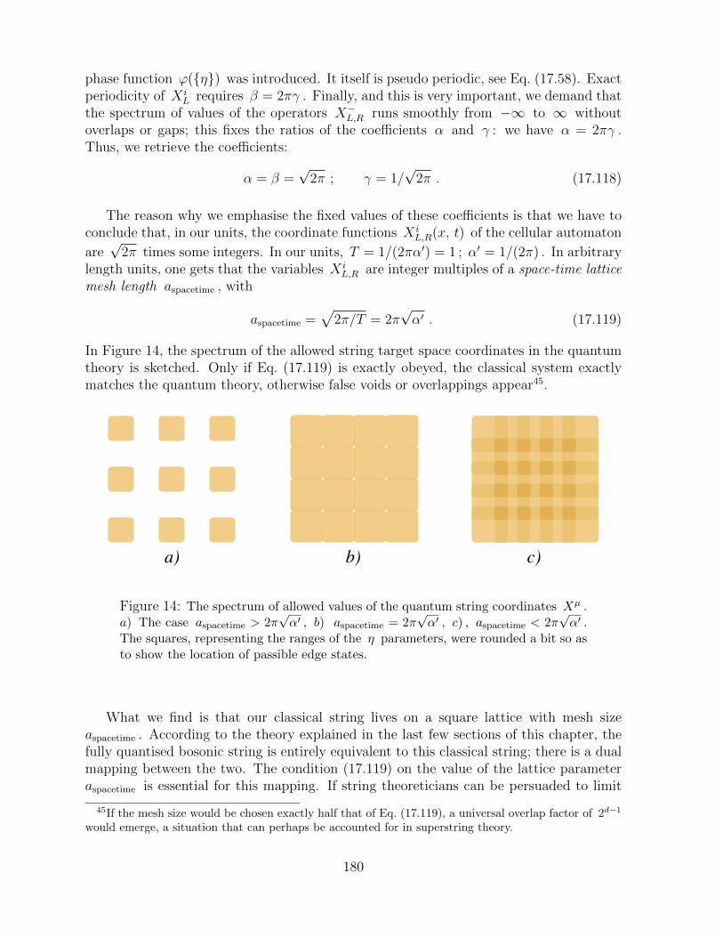
phase function ϕ(η) was introduced. It itself is pseudo periodic, see Eq. (17.58). Exactperiodicity of X i

L requires β = 2πγ . Finally, and this is very important, we demand thatthe spectrum of values of the operators X−L,R runs smoothly from −∞ to ∞ withoutoverlaps or gaps; this fixes the ratios of the coefficients α and γ : we have α = 2πγ .Thus, we retrieve the coefficients:

α = β =√

2π ; γ = 1/√

2π . (17.118)

The reason why we emphasise the fixed values of these coefficients is that we have toconclude that, in our units, the coordinate functions X i

L,R(x, t) of the cellular automaton

are√

2π times some integers. In our units, T = 1/(2πα′) = 1 ; α′ = 1/(2π) . In arbitrarylength units, one gets that the variables X i

L,R are integer multiples of a space-time latticemesh length aspacetime , with

aspacetime =√

2π/T = 2π√α′ . (17.119)

In Figure 14, the spectrum of the allowed string target space coordinates in the quantumtheory is sketched. Only if Eq. (17.119) is exactly obeyed, the classical system exactlymatches the quantum theory, otherwise false voids or overlappings appear45.

c)b)a)

Figure 14: The spectrum of allowed values of the quantum string coordinates Xµ .a) The case aspacetime > 2π

√α′ , b) aspacetime = 2π

√α′ , c) , aspacetime < 2π

√α′ .

The squares, representing the ranges of the η parameters, were rounded a bit so asto show the location of passible edge states.

What we find is that our classical string lives on a square lattice with mesh sizeaspacetime . According to the theory explained in the last few sections of this chapter, thefully quantised bosonic string is entirely equivalent to this classical string; there is a dualmapping between the two. The condition (17.119) on the value of the lattice parameteraspacetime is essential for this mapping. If string theoreticians can be persuaded to limit

45If the mesh size would be chosen exactly half that of Eq. (17.119), a universal overlap factor of 2d−1

would emerge, a situation that can perhaps be accounted for in superstring theory.

180

themselves to string coordinates that live on this lattice, they will see that the completeset of quantum states of the bosonic string still spans the entire Hilbert space they areused to, while now all basis elements of this Hilbert space propagate classically, accordingto the discrete analogues of the classical string equations.

Intuitively, in the above, we embraced the lattice theory as the natural ontologicalsystem corresponding to a non-interacting string theory in Minkowski space. However, inprinciple, we could just as well have chosen the compactified theory. This theory wouldassert that the transverse degrees of freedom of the string do not live on R d−1 , but onT d−1 , a (continuous) torus in d − 1 dimensions, again with periodicity conditions overlengths 2π

√α′ , and these degrees of freedom would move about classically.

In subsection 17.3.5 we elaborate further on the nature of the deterministic stringversions.

17.3.3. The lowest string excitations

String theory is a quantum field theory on the 1 + 1 dimensional world sheet of thestring. If this quantum field theory is in its ground state, the corresponding string modedescribes the lightest possible particle in this theory. As soon as we put excited statesin the world sheet theory, the string goes into excited states, which means that we aredescribing heavier particles. This way, one describes the mass- or energy spectrum of thestring.

In the original versions of the theory, the lightest particle turned out to have a negativemass squared; it would behave as a tachyon, which would be an unwanted feature of atheory.

The more sophisticated, modern versions of the theory are rearranged in such a waythat the tachyon mode can be declared to be unphysical, but it still acts as a descriptionof the formal string vacuum. To get the string spectrum, one starts with this unphysicaltachyon state and then creates descriptions of the other states by considering the actionof creation operators.

To relate these string modes to the ontological states at the deterministic, classicalsides of our mapping equation, we again consider the ground state, as it was described insubsection 17.1.5, to describe the tachyon solution. Thus, the same procedure as in thatsubsection will have to be applied. Similarly one can get the physical particles by havingthe various creation operators act on the tachyon (ground) state. This way, we get ourdescription of the photon (the first spin one state of the open string) and the graviton(the spin 2 excited state of the closed string).

17.3.4. The Superstring

To construct theories containing fermions, it was proposed to plant fermionic degrees offreedom on the string world sheet. Again, anomalies were encountered, unless the bosonicand fermionic degrees of freedom can be united to form super multiplets. Each bosoniccoordinate degree of freedom Xµ(σ, τ) would have to be associated with a fermionic degree

181

of freedom ψµ(σ, τ) . This should be done for the left-moving modes independently of theright-moving ones. A further twist can be given to the theory by only adding fermionicmodes to the left-movers, not to the right movers (or vice versa); this way, chirality can beintroduced in string theory, not unlike the chirality that is clearly present in the StandardModel. Such a theory is called a heterotic string theory.

Since the world sheet is strictly two-dimensional, we have no problems with spin andhelicity within the world sheet, so, here, the quantisation of fermionic fields — at least atthe level of the world sheet — is simpler than in the case of the ‘neutrinos’ discussed insubsection 15.2.3.

Earlier, we used the coordinates σ and τ as light cone coordinates on the world sheet;now, temporarily, we want to use there a space-like coordinate and a time-like one, whichwe shall call x1 = x and x0 = t .

On the world sheet, spinors are 2-dimensional rather than 4-dimensional, and we takethem to be hermitean operators, called Majorana fields, which we write as

ψµ∗(x, t) = ψµ(x, t) , and ψµ†(x, t) = ψµ ∗T (x, t) (17.120)

(assuming a real Minkowskian target space; the superscripts ∗T mean that if ψ = (ψ1

ψ2)

then ψ∗T = (ψ∗1, ψ∗2) ).

There are only two Dirac matrices, call them %0 and %1 , or, after a Wick rotation,%1 and %2 . They obey

%0 = i%2 , %α, %β = %α%β + %β%α = 2ηαβ , (α, β = 1, 2) . (17.121)

A useful representation is

%1 = σx =

(0 11 0

), %2 = σy =

(0 −ii 0

); %0 =

(0 1−1 0

). (17.122)

The spinor fields conjugated to the fields ψµ(x, t) are ψµ(x, t) , here defined by

ψµ

= ψµT%2 , (17.123)

Skipping a few minor steps, concerning gauge fixing, which can be found in the text booksabout superstrings, we find the fermionic part of the Lagrangian:

L(x, t) = −d∑

µ=0

ψµ(x, t) %α∂α ψ

µ(x, t) . (17.124)

Since the %2 is antisymmetric and fermion fields anti-commute, two different spinorsψ and χ obey

χψ = χT%2ψ = i(−χ1ψ2 + χ2ψ1) = i(ψ2χ1 − ψ1χ2) = ψT%2χ = ψχ . (17.125)

Also we have

χ%µψ = −ψ%µχ , (17.126)

182

an antisymmetry that explains why the Lagrangian (17.124) is not a pure derivative. TheDirac equation on the string world sheet is found to be

2∑α=1

%α∂αψµ = 0 . (17.127)

In the world sheet light cone frame, one writes

(%+∂− + %−∂+)ψ = 0 , (17.128)

where, in the representation (17.122),

%± = 1√2(%0 ± %1) , and (17.129)

%+ = −%− =√

2

(0 01 0

), %− = −%+ =

√2

(0 −10 0

). (17.130)

The solution of Eq. (17.127) is simply

ψµ(σ, τ) =

(ψµL(σ)

ψµR(τ)

). (17.131)

Thus, one finds that the fermionic left-movers and right-movers have no further spinorindices.

As is the case for the bosonic coordinate fields XµL,R(x) , also the fermionic field com-

ponents ψµL,R have two longitudinal modes, µ = ± , that are determined by constraintequations. These equations are dictated by supersymmetry. So for the fermions also, weonly keep the d − 1 transverse components as independent dynamical fields ( d is thenumber of space-like dimensions in target space).

The second-quantised theory for such fermionic fields has already briefly been discussedin our treatment of the second-quantised ‘neutrino’ system, in section 15.2.3. Let us repeathere how it goes for these string world sheet fermions. Again, we assume a lattice on theworld sheet, while the Dirac equation on the lattice now reduces to a finite-step equation,so chosen as to yield exactly the same solutions (17.131):

ψi(x, t) = − 1√2%0(%+ψi(x− 1, t− 1) + %−ψi(x+ 1, t− 1)

),

i = 1, · · · , d− 1 . (17.132)

The deterministic counterpart is a Boolean variable set si(x, t) , which we assume to betaking the values ±1 . One may write their evolution equation as

si(x, t) = si(x− 1, t− 1) si(x+ 1, t− 1) si(x, t− 2) . (17.133)

of which the solution can be written as

si(x, t) = siL(x, t) siR(r, t) , (17.134)

183

where siL and siR obey

siL(x, t) = siL(x+ 1, t− 1) ; siR(x, t) = siR(x− 1, t− 1) , (17.135)

which is the Boolean analogue of the Dirac equation (17.132).

One can see right away that all basis elements of the Hilbert space for the Diracequation can be mapped one-to-one onto the states of our Boolean variables. If we wouldstart with these states, there is a straightforward way to construct the anti-commutingfield operators ψiL,R(x, t) of our fermionic system, the Jordan-Wigner transformation [4],also alluded to in section 15.2.3. At every allowed value of the parameter set (x, i, α) ,where α stands for L or R , we have an operator aiα(x) acting on the Boolean variablesiα(x) as follows:

a|+〉 = |−〉 ; a|−〉 = 0 . (17.136)

These operators, and their hermitean conjugates a† obey the mixed commutation - anti-commutation rules

aiα(x), aiα(x) = 0 , aiα(x), ai†α (x) = I , (17.137)

[aiα(x1), ajβ(x2)] = 0 , [aiα(x1), aj†β (x2)] = 0 if

x1 6= x2

and/or i 6= jand/or α 6= β .

(17.138)

Turning the commutators in Eq. (17.138) into anti-commutators is easy, if one canput the entire list of variables x, i and α in some order. Call them y and consider theordering y1 < y2 . Then, the operators ψ(y) can be defined by:

ψ(y) ≡( ∏y1<y

s(y1))a(y) . (17.139)

This turns the rules (17.137) and (17.138) into the anti-commutation rules for fermionicfields:

ψ(y1), ψ(y2) = 0 ; ψ(y1), ψ†(y2) = δ(y1, y2) . (17.140)

In terms of the original variables, the latter rule is written as

ψiα(x1), ψj†β (x2) = δ(x1 − x2)δijδaβ . (17.141)

Let us denote the left-movers L by α = 1 or β = 1 , and the right movers R by α = 2or β = 2 . Then, we choose our ordering procedure for the variables y1 = (x1, i, α) andy2 = (x2, j, β) to be defined by

if α < β then y1 < y2 ;if α = β and x1 < x2 then y1 < y2 ;

if α = β and x1 = x2 and i < j then y1 < y2 ,else y1 = y2 or y1 > y2 . (17.142)

184

This ordering is time-independent, since all left movers are arranged before all rightmovers. Consequently, the solution (17.131) of the ‘quantum’ Dirac equation holds with-out modifications in the Hilbert space here introduced.

It is very important to define these orderings of the fermionic fields meticulously, as inEqs. (17.142). The sign function between brackets in Eq. (17.139), which depends on theordering, is typical for a Jordan-Wigner transformation. We find it here to be harmless,but this is not always the case. Such sign functions can be an obstruction against morecomplicated procedures one might wish to perform, such as interactions between severalfermions, between right-movers and left-movers, or in attempts to go to higher dimensions(such as in k -branes, where k > 2 ).

At this point, we may safely conclude that our dual mapping between quantised stringsand classical lattice strings continues to hold in case of the superstring.

17.3.5. Deterministic strings and the longitudinal modes

The transverse modes of the (non interacting) quantum bosonic and superstrings (in flatMinkowski space-time) could be mapped onto a deterministic theory of strings movingalong a target space lattice. How do we add the longitudinal coordinates, and how dowe check Lorentz invariance? The correct way to proceed is first to look at the quantumtheory, where these questions are answered routinely in terms of quantum operators.

Now we did have to replace the continuum of the world sheet by a lattice, but weclaim that this has no physical effect because we can choose this lattice as fine as weplease whereas rescaling of the world sheet has no effect on the physics since this is just acoordinate transformation on the world sheet. We do have to take the limit `→∞ butthis seems not to be difficult.

Let us first eliminate the effects of this lattice as much as possible. Rewrite Eqs. (17.5)and (17.6) as:

p(x, t) = ∂xk(x, t) , aL,R(x, t) = ∂xbL,R(x, t) ; (17.143)

bL(x+ t) = k(x, t) + q(x, t) ; bR(x− t) = k(x, t)− q(x, t) ; (17.144)

the new fields now obey the equal time commutation rules

[q(x, t), k(x′, t)] = 12i sgn(x− x′ ) ; (17.145)

[bL(x), bL(y)] = − [bR(x), bR(y)] = −i sgn(x− y) , (17.146)

where sgn(x) = 1 if x > 0 , sgn(x) = −1 if x < 0 and sgn(0) = 0 .

Staying with the continuum for the moment, we cannot distinguish two “adjacent”sites, so there will be no improvement when we try to replace an edge state that is singularat η(x) = ±π by one that is singular when this value is reached at two adjacent sites;in the continuum, we expect our fields to be continuous. In any case, we now drop theattempt that gave us the expressions (17.56) and (17.57), but just accept that there isa single edge state at every point. This means that, now, we replace these mapping

185

equations by

bL(x) =√

2πBLop (x) +

1√2πζLop(x) , (17.147)

bR(x) =√

2πBRop (x) +

1√2πζRop(x) , (17.148)

where the functions BL,R will actually play the role of the integer parts of the coordinatesof the string, and ζL,Rop (x) are defined by their action on the integer valued functionsBL,R(x) , as follows:

eiζL(x1)|BL,R(x)〉 = |B′L,R(x)〉 ,

B′L(x) = BL(x) + θ(x− x1 ) ,B′R(x) = BR(x) ;

(17.149)

eiζR(x1)|BL,R(x)〉 = |B′′L,R(x)〉 ,

B′′L(x) = BL(x) ,B′′R(x) = BR(x) + θ(x1 − x) ,

(17.150)

so that, disregarding the edge state,

[BL(x), ζL(y)] = −iθ(x− y) , [BR(x), ζR(y)] = −iθ(y − x) . (17.151)

This gives the commutation rules (17.146). If we consider again a lattice in x space, wherethe states are given in the ζ basis, then the operator BL

op(x) obeying commutation rule(17.151) can be written as

BLop(x1) =

∑y<x1

−i ∂

∂ζL(y). (17.152)

Now the equations of motion of the transverse string states are clear. These justseparate into left-movers and right-movers, both for the discrete lattice sites X i(σ, τ)and for the periodic ηi(σ, τ) functions, where i = 1, · · · , d − 1 . Also, the longitudinalmodes split up into left moving ones and right moving ones. These, however, are fixedby the gauge constraints. In standard string theory, we can use the light cone gauge topostulate that the coordinate variable X+ is given in an arbitrary way by the world sheetcoordinates, and one typically chooses the constraint equations (17.101).

This means that

a+L(σ) = 1 , a+

R(τ) = 1 , (17.153)

but by simple coordinate transformations σ → σ1(σ) and τ → τ1(τ) , one can chooseany other positive function of the coordinate σ (left-mover) or τ (right mover). Now,Eqs. (17.95) here mean that

(aµL(σ))2 = (aµR(τ))2 = 0 , (17.154)

so that, as in Eqs. (17.102) and (17.103), we have the constraints

a+L(σ) = 1

2

d−1∑i=1

(aiL(σ))2 , a+R(τ) = 1

2

d−1∑i=1

(aiR(t))2 , (17.155)

186

where aiL,R(x) = ∂xbiR,L(x) (see the definitions 17.143).

In view of Eq. (17.152) for the operator BiL(x) , it is now tempting to write for the

longitudinal coordinate X+L : ∂σB

iL(σ) = −i ∂

∂ζiL(σ), so that

∂σX+L (σ)

?= 1

2

d−1∑i=1

(− 2π ∂2

∂ζ(σ)2+

1

2π(∂σζ(σ))2 − 2i ∂

∂ζ(σ), ∂σζ(σ)

), (17.156)

but the reader may have noticed that we now disregarded the edge states, which heremay cause problems: they occur whenever the functions ηi cross the values ±π , wherewe must postulate periodicity.

We see that we do encounter problems if we want to define the longitudinal coordi-nates in the compactified classical field theory. Similarly, this is also hard in the discreteautomaton model, where we only keep the Bi

L,R as our independent ontological variables.How do we take their partial derivatives in σ and τ ?

Here, we can bring forward that the gauge conditions (17.153) may have to be replacedby Dirac delta functions, so as to reflect our choice of a world sheet lattice.

These aspects of the string models we have been considering are not well understood.This subsection was added to demonstrate briefly what happens if we study the gaugeconstraints of the theory to get some understanding of the longitudinal modes, in terms ofthe ontological states. At first sight it seemed that the compactified deterministic theorywould offer better chances to allow us to rigorously derive what these modes look like; itseems as if we can replace the world sheet lattice by a continuum, but the difficulties arenot entirely resolved.

If we adopt the cellular automaton based on the integers BiL,R , use of a world sheet

lattice is almost inevitable. On the world sheet, the continuum limit has to be taken withmuch care.

17.3.6. Some brief remarks on (super) string interactions

As long as our (super) strings do not interact, the effects of the constraints are minor.They tell us what the coordinates X−(σ, τ) are if we know all other coordinates on theworld sheet. In the previous section, our point was that the evolution of these coordinateson the world sheet is deterministic. Our mappings from the deterministic string statesonto the quantum string states is one-to-one, apart from the edge states that we chooseto ignore. In the text books on string theory, superstring interactions are described byallowing topologically non-trivial world sheets. In practice, this means that strings mayexchange arms when they meet at one point, or their end points may join or tear apart.All this is then controlled by a string coupling constant gs ; an expansion in powers of gsyields string world sheet diagrams with successively higher topologies.

Curiously, one may very well imagine a string interaction that is deterministic, exactlyas the bulk theory obeys deterministic equations. Since, in previous sections, we did notrefer to topological boundary conditions, we regard the deterministic description obtainedthere as a property of the string’s ‘bulk’.

187

A natural-looking string interaction would be obtained if we postulate the following:

Whenever two strings meet at one point on the space-time lattice, they ex-change arms, as depicted in Fig. 15.

This “law of motion” is deterministic, and unambiguous, provided that both strings areoriented strings. The deterministic version of the interaction would not involve any freelyadjustable string constant gs .

If we did not have the problem how exactly to define the longitudinal componentsof the space-time coordinates, this would complete our description of the deterministicstring laws. Now, however, we do have the problem that the longitudinal coordinatesare ‘quantum’; they are obtained from constraints that are non-linear in the other fieldsXµ(σ, τ) , each of which contain integer parts and fractional parts that do not commute.

Figure 15: Deterministic string interaction. This interaction takes place whenevertwo pieces of string meet at one space-time point.

This problem, unfortunately, is significant. It appears to imply that, in terms of the‘deterministic’ variables, we cannot exactly specify where on the world sheet the exchangedepicted in Figure 15 takes place. This difficulty has not been resolved, so as yet we cannotproduce a ‘deterministic’ model of interacting ‘quantum’ strings.

We conclude from our exercise in string theory that strings appear to admit a descrip-tion in terms of ontological objects, but just not yet quite. The most severe difficulties liein the longitudinal modes. They are needed to understand how the theory can be madeLorentz invariant. It so happens that local Lorentz invariance is a problem for everytheory that attempts to describe the laws of nature at the Planck scale, so it should notcome as a surprise that we have these problems here as well. We suspect that today’sincomplete understanding of Lorentz invariance at the Planck scale needs to be repaired,but it may well be that this can only be done in full harmony with the Cellular AutomatonInterpretation. What this section suggests us is that this cannot be done solely within theframework of string theory, although strings may perhaps be helpful to lead us to furtherideas.

An example of a corner of string theory that has to be swept clean is the black holeissue. Here also, strings seem to capture the physical properties of black holes partlybut not completely; as long as this is the case one should not expect us to be able toformulate a concise ontological theory. This is why most parts of this book concentrateon the general philosophy of the CAI rather than attempting to construct a completemodel.

188

18. Symmetries

In classical and in quantum systems, we have Noether’s theorem [1]:

Whenever there is a continuous symmetry in a system, there exists a conservedquantity associated with it.

Examples are conservation of momentum (translation symmetry), conservation of energy(symmetry with respect to time translations), and angular momentum (rotation sym-metry). In classical systems, Noether’s theorem is limited to continuous symmetries, inquantum systems, this theorem is even more universal: here also discrete symmetries havetheir associated conservation laws: parity P = ±1 of a system or particle (mirror sym-metry), non commuting discrete quantum numbers associated with more general discretepermutations, etc. Also, in a quantum system, one can reverse the theorem:

Every conserved quantity is associated to a symmetry,

for instance isospin symmetry follows from the conservation of the isospin vector ~I =(I1, I2, I3) , baryon number conservation leads to a symmetry with respect to U(1) rota-tions of baryonic wave functions, and so on.

18.1. Classical and quantum symmetries

We now claim that this more generalised Noether theorem can also be applied to classicalsystems, simply by attaching a basis element of Hilbert space to every state the classicalsystem can be in. If, for instance, the evolution law Ut, t+δt is independent of time t , wehave a conserved energy. This energy is obtained from the eigenvalue of Ut, t+δt for thesmallest admissible value of δt . Now since an energy eigenstate will usually not be anontological state of the system, this energy conservation law only emerges in our quantumprocedure; it does not show up in standard classical considerations. For us, this is veryimportant: if δt is as small as the Planck time, the energy eigenstates, all the way tothe Planck energy, are superpositions of ontological states. If, as we usually do, we limitourselves to quantum systems with much lower energies, we are singling out a section ofHilbert space that is not represented by individual ontological states, and for this reasonwe should not expect recognisable classical features in the quantum systems that we areusually looking at: atoms, molecules, elementary particles.

Often, our deterministic models are based on a lattice rather than a space-time con-tinuum. The classical space-time symmetries on a lattice are more restricted than thoseof a continuum. It is here that our mappings onto quantum systems may help. If weallow ontological states to have symmetry relations with superimposed states, much moregeneral symmetry groups may be encountered. This is further illustrated in this chapter.

Since we often work with models having only finite amounts of data in the form ofbits and bytes in given volume elements, we are naturally led to systems defined on alattice. There are many ways in which points can be arranged in a lattice configuration,

189

as is well known from the study of the arrangement of atoms in crystalline minerals. Thesymmetry properties of the minerals are characterised by the set of crystallographic pointgroups, of which there are 32 in three dimensions. [46]

The simplest of these is the cubic symmetry group generated by a cubic lattice:

~x = (n1, n2, n3) , (18.1)

where n1, n2 and n3 are integers. What we call the cubic group here, is the set of all 48orthogonal rotations including the reflections of these three integers into ± each other (6permutations and 23 signs). This group, called O(3,Z) , is obviously much smaller thanthe group O(3,R) of all orthonormal rotations. The cubic group is a finite subgroup ofthe infinite orthogonal group.

Yet in string theory, section 17.3.2, something peculiar seems to happen: even thoughthe string theory is equivalent to a lattice model, it nevertheless appears not to lose itsfull orthogonal rotation symmetry. How can this be explained?

18.2. Continuous transformations on a lattice

Consider a classical model whose states are defined by data that can be arranged in a d di-mensional cubic lattice. Rotation symmetry is then usually limited by the group O(d,Z) .If now we introduce our Hilbert space, such that every state of the classical system is abasis element of that, then we can introduce superpositions, and much more symmetrygroups are possible. There are several ways now to introduce continuous translations androtations.

To this end, it is, again, very instructive to do the Fourier transformation:

〈~x|ψ〉 = (2π)−d/2∫|κi|<π

dd~κ〈~κ|ψ〉ei~κ·~x , (18.2)

Here, |ψ〉 describes a single particle living on the lattice, but we could also take it asthe operator field of a second-quantised system, as is usual in quantum field theories. Ofcourse, as is usual in physics notation, 〈~x| are the bras in x space (where ~x is Eq. (18.1),the lattice), whereas 〈~κ| are the bras in momentum space, where ~κ are continuous, andall its components κi obey |κi| < π .

The inverse of the Fourier transform (18.2) is:

〈~κ|ψ〉 = (2π)−d/2∑~x∈Zd〈~x|ψ〉 e−i~κ·~x . (18.3)

18.2.1. Continuous translations

Translations over any distance ~a can now be defined as the operation

〈~κ|ψ〉 → 〈~κ|ψ〉 e−i~κ·~a , (18.4)

190

although only if ~a has integer components, this represents an ontological shift

〈~x|ψ〉 → 〈 ~x− ~a |ψ〉 , (18.5)

since ~x must sit in the lattice, otherwise this would represent a non ontological state.

If ~a has fractional components, the translation in x space can still be defined. Takefor instance a fractional value for ax , or, ~a = (ax, 0, 0) . Then

〈κx|ψ〉 → 〈κx|ψ〉 e−iκxax , 〈x|ψ〉 →∑x′

〈x′|ψ〉∆ax(x− x′) ,

∆ax(x1) = (2π)−1

∫ π

−πdκx e

−iaxκx+iκx x1 =sin π(x1 − ax)π (x1 − ax)

, (18.6)

where we also used Eq. (18.3) for the inverse of Eq. (18.2).

One easily observes that Eq. (18.6) reduces to Eq. (18.5) if ax tends to an integer.Translations over a completely arbitrary vector ~a are obtained as the product of fractionaltranslations over (ax, 0, 0) , (0, ay, 0) and (0, 0, az) :

〈~x|ψ〉 →∑

x′, y′, z′

〈~x ′|ψ〉∆~a(~x− ~x ′) , ∆~a(~x1) = ∆ax(x1)∆ay(y1)∆az(z1) . (18.7)

Notice that the kernel function ∆~a(~x1) maximises for the values of ~x1 closest to ~a ,so, even for translations over fractional values of the components of ~a , the translationoperation involves only the components of |ψ〉 closest to the target value ~x− ~a .

The generator for infinitesimal translations is the operator ~η op . Translations over a fi-nite distance ~a can then be described by the operator ei~a·~η op . Writing ~η op = (ηx, ηy, ηz) ,and taking ηx, ηy, and ηz each to act only in one dimension, we have

〈~κ| ~η op |ψ〉 = −~κ 〈~κ|ψ〉 , (18.8)

〈x| eiηx ax|ψ〉 =∑x′

〈x′|ψ〉 sin π(x− x′ − ax)π(x− x′ − ax)

, (18.9)

and when ax is taken to be infinitesimal, while x and x′ are integers, one finds

〈x|(I + iηxax)|ψ〉 =∑x′

〈x′|ψ〉(δxx′ + (1− δxx′)

(−1)x−x′(−πax)

π(x− x′)

); (18.10)

〈x| ηx |x〉 = 0 , 〈x| ηx |x′〉 =i (−1)x−x

′

x− x′if x 6= x′ . (18.11)

The eigenstates |ηx〉 of the operator ηx can be found: 〈x|ηx〉 = e−iηxx .

The expressions we found for this generator are the most natural ones but not theonly possible choices; we must always remember that one may add multiples of 2π to itseigenvalues. This modifies the matrix elements (18.11) while the effects of translationsover integer distances remain the same.

191

An important feature of our definition of fractional translations on a lattice is theircommutation rules. These translations are entirely commutative (as we can deduce fromthe definition Eq. (18.4)):

[~η, ~η ′] = 0 . (18.12)

18.2.2. Continuous rotations 1: Covering the Brillouin zone with circular regions

What can be done with translations on a lattice, can also be done for rotations, in variousways. Let us first show how to obtain a perfect general rotation operator on a lattice, inprinciple. Again, we start from the Fourier modes, eiκx , Eq. (18.2). How do we generatearbitrary rotations?

Taking again the cubic lattice as our prototype, we immediately see the difficulty: thespace of allowed values for ~κ is a square (in 2 dimensions) or a cube (in 3 dimensions).This square and this cube are only invariant under the discrete rotation group O(d,Z) .Therefore, rotations over other angles can at best be approximate, it seems. We illustratethe situation for a two-dimensional square lattice, but extrapolation to d > 2 spacedimensions and/or other lattice configurations is straightforward.

The space of allowed momentum values is called the Brillouin zone, and it is thesquare in Figure 16 a . A first approximation for a rotation of the lattice by any angleϕ is obtained by drawing the largest possible circle in the Brillouin zone (or the largestpossible sphere in the 3 or higher dimensional case) and rotate the region inside that. Thedata on the remainder of the Brillouin zone, outside the circle, are ignored or replaced byzero.

This procedure perhaps looks good for the lower frequency modes, but it does notrotate everything, and it would clearly disobey the desired group properties of rotationsand translations, so we must do something better with the remainder of the Brillouin zone.This is possible, see Fig 16 b . The rotation operator could then be defined as follows.

We fill the entire Brillouin zone with circular regions, such that they completely coverthe entire space without overlappings. As will be explained shortly, we prefer to keep thesecircles as large as possible to get the best46 result. The action of the rotation operatorwill now be defined to correspond to a rotation over the same angle ϕ inside all of thesecircles (arrows in Figs. 16 a and b ). With “circles” we here mean circular regions, or, ifd > 2 , regions bounded by (d− 1) -spheres.

This is – nearly47 – the best we can do in the Brillouin zone, being the space of theFourier vectors ~κ . The reason why we split the Brillouin zones into perfectly sphericalregions, rather than other shapes, becomes clear if we inspect the action of this operatorin ~x -space: how does this operator work in the original space of the lattice sites ~x ?

Let us first consider the action of a single circle, while the data on the rest of theBrillouin zone are replaced by zero. First take a circle (if d = 2 ) or sphere (if d = 3 )

46“best” here means that the effect of the rotation is maximally local, as will be seen in the sequel.47A slight complication that can be cured, is explained shortly after Eq. (18.19) on page 195.

192

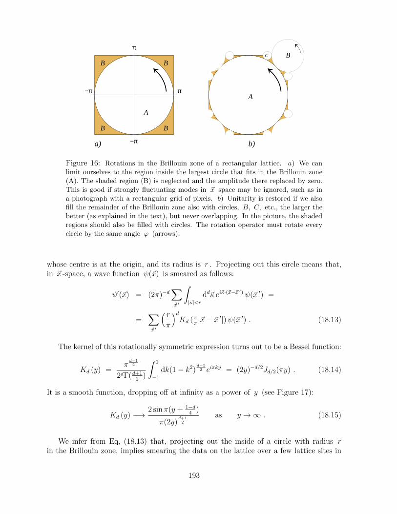
π

−π

π−π

BB

BB

A

B

A

C

b)a)

Figure 16: Rotations in the Brillouin zone of a rectangular lattice. a) We canlimit ourselves to the region inside the largest circle that fits in the Brillouin zone(A). The shaded region (B) is neglected and the amplitude there replaced by zero.This is good if strongly fluctuating modes in ~x space may be ignored, such as ina photograph with a rectangular grid of pixels. b) Unitarity is restored if we alsofill the remainder of the Brillouin zone also with circles, B, C, etc., the larger thebetter (as explained in the text), but never overlapping. In the picture, the shadedregions should also be filled with circles. The rotation operator must rotate everycircle by the same angle ϕ (arrows).

whose centre is at the origin, and its radius is r . Projecting out this circle means that,in ~x -space, a wave function ψ(~x) is smeared as follows:

ψ′(~x) = (2π)−d∑~x ′

∫|~κ|<r

dd~κ ei~κ·(~x−~x′) ψ(~x ′) =

=∑~x ′

( rπ

)dKd ( r

π|~x− ~x ′|)ψ(~x ′) . (18.13)

The kernel of this rotationally symmetric expression turns out to be a Bessel function:

Kd (y) =πd−12

2dΓ(d+12

)

∫ 1

−1

dk(1− k2)d−12 eiπky = (2y)−d/2Jd/2(πy) . (18.14)

It is a smooth function, dropping off at infinity as a power of y (see Figure 17):

Kd (y) −→2 sinπ(y + 1−d

4)

π(2y)d+12

as y →∞ . (18.15)

We infer from Eq, (18.13) that, projecting out the inside of a circle with radius rin the Brillouin zone, implies smearing the data on the lattice over a few lattice sites in

193

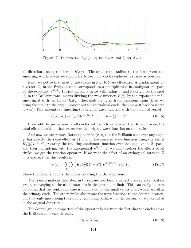
543210-1 y

b

a

Figure 17: The function Kd (y) , a) for d = 2 , and b) for d = 5 .

all directions, using the kernel Kd(y) . The smaller the radius r , the further out thesmearing, which is why we should try to keep our circles (spheres) as large as possible.

Next, we notice that most of the circles in Fig. 16 b are off-centre. A displacement bya vector ~κ1 in the Brillouin zone corresponds to a multiplication in configuration spaceby the exponent ei~κ1·~x . Projecting out a circle with radius r and its origin on the spot~κ1 in the Brillouin zone, means dividing the wave function ψ(~x) by the exponent ei~κ1·~x ,smearing it with the kernel Kd(y) , then multiplying with the exponent again (thus, webring the circle to the origin, project out the centralised circle, then move it back to whereit was). This amounts to smearing the original wave function with the modified kernel

Kd (y,~κ1) = Kd (y)ei~κ1·(~x−~x′) , y = r

π|~x− ~x ′| . (18.16)

If we add the projections of all circles with which we covered the Brillouin zone, thetotal effect should be that we recover the original wave function on the lattice.

And now we can rotate. Rotating a circle (r, κ1) in the Brillouin zone over any angleϕ has exactly the same effect as 1) finding the smeared wave function using the kernelKd (y) e−i~κ1·~x

′, rotating the resulting continuous function over the angle ϕ in ~x -space,

and then multiplying with the exponential ei~κ1·~x . If we add together the effects of allcircles, we get the rotation operator. If we want the effect of an orthogonal rotation Ωin ~x -space, then this results in

ψ′(~x) =∑~x ′

∑i

Kd (riπ|Ω~x− ~x ′|) ei~κi·(~x−~x ′) ψ(~x ′) , (18.17)

where the index i counts the circles covering the Brillouin zone.

The transformations described in this subsection form a perfectly acceptable rotationgroup, converging to the usual rotations in the continuum limit. This can easily be seenby noting that the continuum case is dominated by the small values of ~κ , which are all inthe primary circle. The other circles also rotate the wave functions to the desired location,but they only move along the rapidly oscillating parts, while the vectors ~κ1 stay orientedin the original direction.

The desired group properties of this operator follow from the fact that the circles coverthe Brillouin zone exactly once.

Ω3 = Ω1Ω2 . (18.18)

194

Of course, the operation (18.17), to be referred to as R(Ω) , is not quite an ordinary rota-tion. If T (~a) is the translation over a non-lattice vector ~a as described in section 18.2.1,then

R(Ω)T (~a) 6= T (Ω~a)R(Ω) , (18.19)

and furthermore, if Ω is chosen to be one of the elements of the crystal group of thelattice, R(Ω) does still not coincide with Ω itself. This latter defect can be cured, butwe won’t go into these details.

The best feature of this rotation operator is that it appears to act really locally in~x -space, spreading the lattice points only slightly with the Bessel function kernels (18.14),but it also has disadvantages: it will be extremely difficult to construct some deterministicevolution law that respects this transformation as a symmetry. For this reason, we nowconsider other continuous transformation prescriptions that yield rotations.

18.2.3. Continuous rotations 2: Using Noether charges and a discrete sub group

In a deterministic theory then, we wish to identify an evolution law that respects oursymmetries. This requires a different choice for the definitions of the symmetries involved.To this end, we enter Noether’s theorem, as it was introduced at the beginning of thischapter. For example, symmetry under time translations is associated to the conservationof energy, translation symmetry is associated to momentum conservation, and rotationsymmetry leads to the conservation of angular momentum. We refer to these conservedquantities as Noether charges. All these conserved charges are observable quantities,and therefore, if we wish to investigate them in a quantum theory that we relate toa deterministic system, then this deterministic system should also exhibit observablequantities that can be directly related to the Noether charges.

In the PQ formalism, the Noether charges for translation symmetry are built in, in asense. Translations in the Qi variables are associated to quantities pi , of which the integerparts Pi are ontological observables. Only the fractional parts generate translations,which then must be integer steps on the Q lattice. We need both components of themomentum. If the lattice length is small, the quanta of the integer parts of the momentaare large. Planets have very large momenta, cold atoms have very small momenta. Largemomenta also are sources of gravitational fields, and as such directly observable. Whatabout the transition region? It happens to be in a very familiar domain – the Planck unitof momentum is ∼ 6.5 kg m/sec . Momentum in that domain must be a mixture of theP observables and the Q displacement operators, whereas in ordinary physics we noticenothing special in that domain.

In the case of angular momentum, we may note that angular momentum is quantisedanyway. Can we associate an ontological observable (beable) to angular momentum? Notso easily, because angular momentum consists of non-commuting components. At bestwe will have ontological quantised variables playing the role of “the classical parts” ofangular momentum, supplemented by quantum degrees of freedom (changeables) thatrestore the commutation rules. We observe that, for small particles, angular momentum

195

is only partly observable; sometimes it is a beable, sometimes a changeable. For largesystems, angular momentum is observable, with some margin of error.

This leads us to consider the following structure – and indeed we will have to usesimilar methods whenever a symmetry group becomes large, meaning that it has verymany elements. Since angular momenta are non commutative, they cannot be quiteontological, but their ‘classical parts’ must be. Therefore, we assume that the totalangular momenta operators Ji can be written as follows:

Ji = Li + λi , [Ji, Jj] = iεijkJk , (18.20)

where Li represents the expectation values of Ji in all ontological states, so that Liare beables. The λi represent the remainder, and their expectation values in ontologicalstates vanish:

〈ont|λi|ont〉 = 0 for each ontological state |ont〉 . (18.21)

The following subsection will show an explicit procedure to obtain Li and λi .

18.2.4. Continuous rotations 3: Using the real number operators p and q con-structed out of P and Q

If our theory is defined on a lattice, there is another great way to recover many of thesymmetries of the continuum case, by using the PQ trick as it was exposed in section 16.We saw that string theory, section 17.3, was re-written in such a way that the stringmoves on a lattice in target space, where the lattice basically describes the integer partsof the coordinates, while the space in between the lattice sites actually correspond tothe eigenstates of the displacement operators for the momentum variables P . Together,they form a continuum, and since the entire system is equivalent to the continuum stringtheory, it also shares all continuous translation and rotation symmetries with that theory.

By allowing the application of this mechanism, string theory appears to be morepowerful than theories of point particles; the commutation rules for the operators intarget space are fundamentally different, and string theory allows target space to be in ahigh number of dimensions.

Thus, in the PQ formalism, we now use the continuum definition of angular momen-tum. Consider the wave function of a single particle in three space dimensions, so thatit lives on the product of three P, Q lattices. These lattices generate the three quantumcoordinates qi . Its Hilbert space H is the product space of three Hilbert spaces H1, H2

and H3 .

Write, as in Eqs. (16.18) and (16.19),

qopi = Qi + aop

i , popi = 2πPi + bop

i , (18.22)

so that the angular momentum operator is (in the 3-dimensional case)

Ji = εijkqopj pop

k = εijk(2πQjPk + 2πaopj Pk +Qjb

opk + aop

j bopk ) . (18.23)

196

Since the expectation values of aopi and bop

i vanish in the ontological states, |ont〉 =

|~P , ~Q〉 , and since the last term will be ≤ O(2π) , we can identify Li with the first term:

Li ≈ 2π εijkQjPk . (18.24)

Note, that the Li are quantised in multiples of 2π rather than one, as one might haveexpected, so Eq. (18.24) cannot hold exactly.

Let us now inspect the modifications on the commutation rules of these angular mo-mentum operators caused by the edge states. In each of the three Hilbert spaces Hi ,i = 1, 2, 3, , we have Eq. (16.22), while the operators of one of these Hilbert spacescommute with those of the others. Writing the indices explicitly:

[q1, p1] = i I2I3 ( I1 − |ψ1e〉〈ψ1

e | ) , [q1, p2] = 0 , and cyclic permutations, (18.25)

where Ii are the identity operators in the ith Hilbert space, and |ψie〉 are the edge stateson the ith P, Q lattice. One then easily derives that the three angular momentumoperators Ji defined in the usual way, Eq. (18.23), obey the commutation rules

[J1, J2] = iJ3 I1I2 ( I3 − |ψ3e〉〈ψ3

e | ) , and cyclic permutations. (18.26)

The importance of this result is that now we observe that the operator J3 only acts inHilbert spaces 1 and 2, but is proportional to the identity in H3 (since J3 contains onlyq1, q2, p1, and p2 ). So the projection operator for the edge state |ψ3

e〉 commutes with J3 .This implies that, if we limit ourselves to states that are orthogonal to the edge states, theywill also rotate to states orthogonal to the edge states. In this subspace of Hilbert spacethe rotations act normally. And we think that this is remarkable, because certainly the“ontological” basis defined on the six-dimensional ~P , ~Q lattice has no built-in continuousrotation invariance at all.

18.2.5. Quantum symmetries and classical evolution

In previous subsections it was observed that, when we project classical models on Hilbertspaces, new symmetries may emerge. These are symmetry transformations that mapclassical states onto superpositions of states. A few examples were shown.

None of our procedures are fool proof. In the special case to be discussed next, westudy time translation invariance. As stated earlier, we might split the energy E into aclassical part ( δE ) and a quantum part (the generator of discrete time translations, theHamiltonian H that lies in the interval [0, 2π/δt) . However, this would suggest that wecan only measure energies with 2π/δt as our margin of error. That cannot be right: ifδt is the Planck time, then the energy quantum is the Planck energy, EPlanck , which isabout 543 kiloWatt-hours; yet we pay our electricity bills per kiloWatt-hour, and thosebills are certainly ontological. Mutations in our DNA profiles might require only a coupleof electronVolts to take place, and these might be crucial for our genetically inheritedidentities; an electronVolt is about 10−28 times the Planck energy. Even that may haveto be (mostly) ontological.

197

Of course we are primarily interested in symmetries that are symmetries of the evolu-tion operator. The cogwheel model, section 2.2.1, for instance has the classical symmetryof rotations over N steps, if N is the number of cogwheel position states. But if we goto the energy eigenstates |k〉H , k = 0, · · ·N − 1 (Eqs. 2.21 and 2.22), we see that, there,a translation over n teeth corresponds to multiplication of these states as follows:

|k〉H → e2πikn/N |k〉H . (18.27)

Since these are eigenstates of the Hamiltonian, this multiplication commutes with H andhence the symmetry is preserved by the evolution law.

We now found out that we can enlarge the symmetry group by choosing the multipli-cation factors in frequency space

|k〉H → e2πikα/N |k〉H . (18.28)

where α now may be any real number, and this also corresponds to a translation in timeover the real number α . This enhances the symmetry group from the group of the cyclicpermutations of N elements to the group of the continuous rotations of a circle.

18.2.6. Quantum symmetries and classical evolution 2

An other rather trivial yet interesting example of a symmetry that is enlarged if we applyour quantum constructions, occurs in a simple cellular automaton in any number d ofspace dimensions. Consider the Boolean variables σ(~x, t) = ±1 distributed over all evensites in a lattice space-time, that is, over all points (~x, t) = (x1, · · · , xd, t) with xi andt all integers, and x1 + · · ·+ xd + t = even.

Let the evolution law be

σ(~x, t+ 1) =( d∏i=1

σ(~x+ ~ei , t) σ(~x− ~ei , t))σ(~x , t− 1) , (18.29)

where ~ei are the unit vectors in the ith direction in d dimensional space. Or: the productof the data on all direct space-time neighbours of any odd site (~x, t) is +1 . This law ismanifestly invariant under time reversal, and we see that it fixes all variables if the dataare given on a Cauchy surface consisting of two consecutive layers in time t, t− 1 . Theclassical model has the manifest translation symmetry over vectors δx = (a1, · · · , ad, τ)with

∑i ai + τ even.

Now let us introduce Hilbert space, and consider the odd lattice sites. On these oddsites, we define the action of changeables σ1(~x1, t1) as follows:

The data on the time frame t = t1 , are kept unchanged;on the time frame t = t1 − 1 , only σ(~x1, t1 − 1) changes sign, and all othersremain unchanged;consequently, according to the evolution law, also on the time frame t = t1+1 ,only σ(~x1, t1 + 1) changes sign, all others stay the same.

198

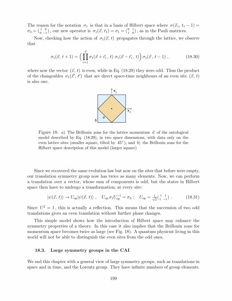
The reason for the notation σ1 is that in a basis of Hilbert space where σ(~x1, t1 − 1) =σ3 = ( 1 0

0 −1) , our new operator is σ1(~x, t1) = σ1 = (0 1

1 0) , as in the Pauli matrices.

Now, checking how the action of σ1(~x, t) propagates through the lattice, we observethat

σ1(~x, t+ 1) =( d∏i=1

σ1(~x+ ~ei , t) σ1(~x− ~ei , t))σ1(~x , t− 1) , (18.30)

where now the vector (~x, t) is even, while in Eq. (18.29) they were odd. Thus the productof the changeables σ1(~x′, t′) that are direct space-time neighbours of an even site (~x, t)is also one.

ba

κx

κy

Figure 18: a) The Brillouin zone for the lattice momentum ~κ of the ontologicalmodel described by Eq. (18.29), in two space dimensions, with data only on theeven lattice sites (smaller square, tilted by 45 ), and b) the Brillouin zone for theHilbert space description of this model (larger square)

Since we recovered the same evolution law but now on the sites that before were empty,our translation symmetry group now has twice as many elements. Now, we can performa translation over a vector, whose sum of components is odd, but the states in Hilbertspace then have to undergo a transformation; at every site:

|ψ(~x, t)〉 → Uop|ψ(~x, t)〉 , Uop σ1U−1op = σ3 ; Uop = 1√

2( 1 1

1 −1) . (18.31)

Since U2 = 1 , this is actually a reflection. This means that the succession of two oddtranslations gives an even translation without further phase changes.

This simple model shows how the introduction of Hilbert space may enhance thesymmetry properties of a theory. In this case it also implies that the Brillouin zone formomentum space becomes twice as large (see Fig. 18). A quantum physicist living in thisworld will not be able to distinguish the even sites from the odd ones.

18.3. Large symmetry groups in the CAI

We end this chapter with a general view of large symmetry groups, such as translations inspace and in time, and the Lorentz group. They have infinite numbers of group elements.

199

Now we imagine our automaton models to have discretised amounts of information spreadover space and time. How can we have infinite and/or continuous symmetry groups acton them?

Our impression from the previous results is that the conventional symmetry generators,as used in quantum theories, will be operators that always consist of combinations ofbeables and changeables: the Noether charges, such as angular momentum, energy andmomentum, will have classical limits that are perfectly observable, hence they are beables;yet quantum mechanically, the operators do not commute, and so there must also bechangeable parts.

The beable parts will be conjugated to the tiniest symmetry operations such as verytiny translations and rotations. These are unlikely to be useful as genuine transformationsamong the ontological data – of course they are not, since they must commute with thebeables.

The changeable parts of these operators are not ontological observables as they do notcommute. The P Q formalism, elaborated in section 16, is a realisation of this concept ofsplitting the operators: here, both in position space and in momentum space, the integerparts of the translation operators are beables, the fractional parts are changeables. Thecontinuous translation operators pop consist of both ingredients. We suspect that thiswill have to become a general feature of all large symmetry groups, in particular theHamiltonian itself, and this is what we shall attempt to implement in the next chapter,19.

19. The discretised Hamiltonian formalism in PQ theory

19.1. The vacuum state, and the double role of the Hamiltonian (cont’d)

The energy conservation law is usually regarded as an interesting and important featureof both classical and quantum mechanics, but it is often not fully realised how importantthe role of this law really is. The importance of energy is that it is conserved, it is definedlocally, and that it cannot be negative48. This allows us to define the vacuum as the singlequantum state of the universe that has the lowest possible energy (or energy per unit ofvolume).

Consider a small perturbation of this vacuum: a light particle, or a grain of dust.It carries only a small amount of energy. In our world, this energy cannot increasespontaneously, because the surrounding vacuum cannot deliver it, and its own energycannot increase. All transitions, all processes inside the grain of dust, can only transformthe object into other states with exactly the same energy. If the object decays, the decayproducts must have even lower amounts of energy. Since the number of distinct states

48Often, the Casimir effect is brought forward as a counter example. Of course, it is important to realisethat this effect can produce small regions of negative energy, but those regions are always accompaniedby domains of much larger amounts of positive energy nearby, so that this effect has little impact on thefundamental issues of stability raised here.

200

with the same or less energy is very limited, not much can happen; the object representsa very stable situation.

But now imagine an alien world where the concept of a conserved, positive energywould not exist. Perhaps our alien world would nevertheless have something like a vacuumstate, but it would have to be defined differently. In this alien world, our tiny object couldgrow spontaneously, since we postulated that there is no conserved quantity such as energyto stop it from doing so. What this means is that the tiniest perturbations around thevacuum state will destabilise this vacuum. Similarly, any other initial state may turn outto be unstable49.

We can state this differently: solutions of the equations of motion are stationary ifthey are in thermal equilibrium (possibly with one or more chemical potentials added).In a thermal equilibrium, we have the Boltzmann distribution:

Wi = C e−βEi+∑j µjRji , (19.1)

where β = 1/kT is the inverse of the temperature T , with Boltzmann constant k , andi labels the states; µj are chemical potentials, and Rji the corresponding conservedquantities.

If the energies Ei were not properly bounded from below, the lowest energies wouldcause this expression to diverge, particularly at low temperatures.

What is needed is a lower bound of the energies Ei so as to ensure stability of ourworld. Furthermore, having a ground state is very important to construct systematic ap-proximations to solutions of the time-independent Schrodinger equation, using extremumprinciples. This is not just a technical problem, it would raise doubt on the mere exis-tence of correct solutions to Schrodinger’s equation, if no procedure could be describedthat allows one to construct such solutions systematically.

In our world we do have a Hamiltonian function, equal to the total energy, that islocally conserved and bounded from below. Note that “locally conserved” means that alocally defined tensor Tµν(~x, t) exists that obeys a local conservation law, ∂µTµν = 0 , andthis feature is connected in important ways not only to the theory of special relativity,but also to general relativity.

Thus, the first role played by the Hamiltonian is that it brings law and order in theuniverse, by being 1) conserved in time, 2) bounded from below, and 3) local (that is, itis the sum of completely localised contributions).

Deriving an equation of motion that permits the existence of such a function, is noteasy, but was made possible by the Hamiltonian procedure, first worked out for continuumtheories (see section 5.6.2 in Part I).

Hamilton’s equations are the most natural ones that guarantee this mechanism towork: first make a judicious choice of kinetic variables xi and pi , then start with any

49The absence of a stabiliser does not imply that a dynamical system has to destabilise; the solarsystem is a classical case in point, it stayed in roughly the same state for billions of years, without anyconspicuous reason for not converting into a more “probable” state. Therefore, the argument presentedhere must be handled with care.

201

function H(xi, pj) that is bounded and local as desired, and subsequently write downthe equations for dxi/dt and dpj/dt that guarantee that dH/dt = 0 . The principle isthen carried over to quantum mechanics in the standard way.

Thus, in standard physics, we have a function or operator called Hamiltonian thatrepresents the conserved energy on the one hand, and it generates the equations of motionon the other.

And now, we argue that, being such a fundamental notion, the Hamiltonian principleshould also exist for discrete systems.

19.2. The Hamilton problem for discrete deterministic systems

Consider now a discrete, deterministic system. Inevitably, time will also be discrete. Timesteps must be controlled by a deterministic evolution operator, which implies that theremust be a smallest time unit, call it δt . When we write the evolution operator U(δt)as U(δt) = e−iE

quant δt then E quant is defined modulo 2π/δt , which means that we canalways choose E quant to lie in the segment

0 ≤ E quant < 2π/δt , (19.2)

Instead, in the real world, energy is an additively conserved quantity without anyperiodicity. In the PQ formalism, we have seen what the best way is to cure such asituation, and it is natural to try the same trick for time and energy: we must add aconserved, discrete, integer quantum to the Hamiltonian operator: E class = 2πN/δt , sothat we have an absolutely conserved energy,

E?= E quant + E class . (19.3)

In the classical theory, we can only use E class to ensure that our system is stable, asdescribed in the previous section.

In principle, it may seem to be easy to formulate a deterministic classical system wheresuch a quantity E class can be defined, but, as we will see, there will be some obstacles ofa practical nature. Note that, if Eq. (19.3) is used to define the total energy, and if E class

reaches to infinity, then time can be redefined to be a continuous variable, since now wecan substitute any value t in the evolution operator U(t) = e−iEt .

One difficulty can be spotted right away: usually, we shall demand that energy be anextensive quantity, that is, for two widely separated systems we expect

E tot = E1 + E2 + E int , (19.4)

where E int can be expected to be small, or even negligible. But then, if both E1 andE2 are split into a classical part and a quantum part, then either the quantum part ofE tot will exceed its bounds (19.2), or E class will not be extensive, that is, it will not evenapproximately be the sum of the classical parts of E1 and E2 .

202

An other way of phrasing the problem is that one might wish to write the total energyE tot as

E tot =∑

lattice sites i

Ei →∫

dd~x H(~x) , (19.5)

where Ei or H(~x) is the energy density. It may be possible to spread E totclass over the

lattice, and it may be possible to rewrite E quant as a sum over lattice sites, but then itremains hard to see that the total quantum part stays confined to the interval [0, 2π/δt)while it is treated as an extensive variable at the same time. Can the excesses be stowedin E int ?

This question will be investigated further in our treatment of the technical details ofthe cellular automaton, chapter 22.

19.3. Conserved classical energy in PQ theory

If there is a conserved classical energy Eclass(~P , ~Q) , then the set of ~P , ~Q values withthe same total energy E forms closed surfaces ΣE . All we need to demand for a theoryin (~P , ~Q) space is that the finite-time evolution operator U(δt) generates motion alongthese surfaces [94]. That does not sound hard, but in practice, to generate evolution lawswith this property is not so easy. This is because we often also demand that our evolutionoperator U(δt) be time-reversible: there must exist an inverse, U−1(δt) .

In classical mechanics of continuous systems, the problem of characterising some evolu-tion law that keeps the energy conserved was solved: let the continuous degrees of freedombe some classical real numbers qi(t), pi(t) , and take energy E to be some function

E = H(~p, ~q ) = T (~p ) + V (~q ) + ~p · ~A(~q ) , (19.6)

although more general functions that are bounded below are also admitted. The lastterm, describing typically magnetic forces, often occurs in practical examples, but maybe omitted for simplicity to follow the general argument.

Then take as our evolution law:

dqidt

= qi =∂H(~p, ~q )

∂pi, pi = −∂H(~p, ~q )

∂qi. (19.7)

One then derives

dH(~p, ~q )

dt= H =

∂H

∂qiqi +

∂H

∂pipi = piqi − qipi = 0 . (19.8)

This looks so easy in the continuous case that it may seem surprising that this principleis hard to generalise to the discrete systems. Yet formally it should be easy to derive someenergy-conserving evolution law:

203

Take a lattice of integers Pi and Qi , and some bounded, integer energyfunction H(~P , ~Q) . Consider some number E for the total energy. Consider

all points of the surface ΣE on our lattice defined by H(~P , ~Q) = E . Thenumber of points on such a surface could be infinite, but let us take the casethat it is finite. Then simply consider a path Pi(t), Qi(t) on ΣE , where tenumerates the integers. The path must eventually close onto itself. This waywe get a closed path on ΣE . If there are points on our surface that are notyet on the closed path that we just constructed, then we repeat the procedurestarting with one of those points. Repeat until ΣE is completely covered byclosed paths. These closed paths then define our evolution law.

At first sight, however, generalising the standard Hamiltonian procedure now seems tofail. Whereas the standard Hamiltonian formalism (19.8) for the continuous case involvesjust infinitesimal time steps and infinitesimal changes in coordinates and momenta, wenow need finite time steps and finite changes. One could think of making finite-sizecorrections in the lattice equations, but that will not automatically work, since odds arethat, after some given time step, integer-valued points in the surface ΣE may be difficultto find. Now with a little more patience, a systematic approach can be formulated, butwe postpone it to section 19.4.

19.3.1. Multi-dimensional harmonic oscillator

A superior procedure will be discussed in the next subsections, but first let us consider thesimpler case of the multi-dimensional harmonic oscillator of section 17.2, subsection 17.2.2:take two symmetric integer-valued tensors Tij = Tji , and Vij = Vji . The evolutionlaw alternates between integer and half-odd integer values of the time variable t . SeeEqs, (17.77) and (17.78):

Qi(t+ 1) = Qi(t) + TijPj(t+ 12) ; (19.9)

Pi(t+ 12) = Pi(t− 1

2)− VijQj(t) . (19.10)

According to Eqs. (17.84), (17.85), (17.88) and (17.89), the conserved classical Hamilto-nian is

H = 12Tij Pi(t+ 1

2)Pj(t− 1

2) + 1

2Vij Qi(t)Qj(t) =

12Tij Pi(t+ 1

2)Pj(t+ 1

2) + 1

2Vij Qi(t)Qj(t+ 1) =

12~P+T ~P+ + 1

2~P+TV ~Q+ 1

2~QV ~Q =

12(~P+ + 1

2~QV )T (~P+ + 1

2V ~Q) + ~Q(1

2V − 1

8V T V ) ~Q =

~P+(12T − 1

8T V T )~P+ + 1

2( ~Q+ 1

2~P+ T )V ( ~Q+ 1

2T ~P+) , (19.11)

where in the last three expressions, ~Q = ~Q(t) and ~P+ = ~P (t + 12) . The equations

(19.11) follow from the evolution equations (19.9) and (19.10) provided that T and Vare symmetric.

204

One reads off that this Hamiltonian is time-independent. It is bounded from below ifnot only V and T but also either V − 1

4V TV or T − 1

4TV T are bounded from below

(usually, one implies the other).

Unfortunately, this requirement is very stringent; the only solution where this energyis properly bounded is a linear or periodic chain of coupled oscillators, as in our one-dimensional model of massless bosons. On top of that, this formalism only allows forstrictly harmonic forces, which means that, unlike the continuum case, no non-linearinteractions can be accommodated for. A much larger class of models will be exhibitedin the next section.

Returning first to our model of massless bosons in 1 + 1 dimensions, section 17, wenote that the classical evolution operator was defined over time steps δt = 1 , and thismeans that, knowing the evolution operator specifies the Hamiltonian eigenvalue op tomultiples of 2π . This is exactly the range of a single creation or annihilation operatoraL,R and aL,R † . But these operators can act many times, and therefore the total energyshould be allowed to stretch much further. This is where we need the exactly conserveddiscrete energy function (19.11). The fractional part of H , which we could call E quant ,follows uniquely from the evolution operator U(δt) . Then we can add multiples of 2πtimes the energy (19.11) at will. This is how the entire range of energy values of our2 dimensional boson model results from our mapping. It cannot be a coincidence thatthe angular energy function E quant together with the conserved integer valued energyfunction E class taken together exactly represent the spectrum of real energy values forthe quantum theory. This is how our mappings work.

19.4. More general, integer-valued Hamiltonian models with interactions

According to the previous section, we recuperate quantum models with a continuous timevariable from a discrete classical system if not only the evolution operator over a timestep δt is time-reversible, but in addition a conserved discrete energy beable E class exists,taking values 2π N/δt where N is integer. Again, let us take δt = 1 . If the eigenvaluesof Uop(δt) are called e−iE

quant, with 0 ≤ E quant < 2π then we can define the complete

Hamiltonian H to be

H = E quant + E class = 2π(ν +N) , (19.12)

where 0 ≤ ν < 1 (or alternatively, − 1/2 < ν ≤ 1/2 ) and N is integer. The quantityconjugated to that is a continuous time variable. If we furthermore demand that E class isbounded from below then Eq. (19.12) defines a genuine quantum system with a conservedHamiltonian that is bounded from below.

As stated earlier, it appears to be difficult to construct explicit, non-trivial examplesof such models. If we try to continue along the line of harmonic oscillators, perhaps withsome non-harmonic forces added, it seems that the standard Hamiltonian formalism failswhen the time steps are finite, and if we find a Hamiltonian that is conserved, it is usuallynot bounded from below. Such models then are unstable; they will not lead to a quantumdescription of a model that is stable.

205

In this section, we shall show how to cure this situation, in principle. We concentrateon the construction of a Hamiltonian principle that keeps a classical energy function E class

exactly conserved in time.

In the multidimensional models, we had adopted the principle that we in turn updateall variables Qi , then all Pi . That has to be done differently. To obtain better models,let us phrase our assignment as follows:

Formulate a discrete, classical time evolution law for some model with the following prop-erties:

i The time evolution operation must be a law that is reversible in time50. Only thenwill we have an operator U(δt) that is unitary and as such can be re-written as theexponent of −i times a hermitean Hamiltonian.

ii There must exist a discrete function E class depending on the dynamical variablesof the theory, that is exactly conserved in time.

iii This quantity E class must be bounded from below.

When these first three requirements are met we will be able to map this system on aquantum mechanical model that may be physically acceptable. But we want more:

iv Our model should be sufficiently generic, that is, we wish that it features interac-tions.

v Ideally, it should be possible to identify variables such as our Pi and Qi so thatwe can compare our model with systems that are known in physics, where we havethe familiar Hamiltonian canonical variables ~p and ~q .

vi We would like to have some form of locality ; as in the continuum system, ourHamiltonian should be described as the integral (or sum) of a local Hamiltoniandensity, H(~x) , and there should exist a small parameter ε > 0 such that at fixedtime t , H(~x) only depends on variables located at ~x ′ with |~x ′ − ~x| < ε .

The last condition turns our system in some discretised version of a field theory ( ~P and~Q are then fields depending on a space coordinate ~x and of course on time t ). One mightthink that it would be hopeless to fulfil all these requirements. Yet there exist beautifulsolutions which we now construct. Let us show how our reasoning goes.

Since we desire an integer-valued energy function that looks like the Hamiltonian of acontinuum theory, we start with a Hamiltonian that we like, being a continuous functionHcont(~q, ~p ) and take its integer part, when also ~p and ~q are integer. More precisely (withthe appropriate factors 2π , as in Eqs. (16.6) and (18.22) in previous chapters): take Pi

50When information loss is allowed, as in section 7 of part I, we shall have to relax this condition.

206

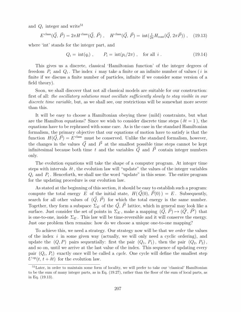
and Qi integer and write51

E class( ~Q, ~P ) = 2πH class( ~Q, ~P ) , H class( ~Q, ~P ) = int( 12πHcont( ~Q, 2π ~P )) , (19.13)

where ‘int’ stands for the integer part, and

Qi = int(qi) , Pi = int(pi/2π) , for all i . (19.14)

This gives us a discrete, classical ‘Hamiltonian function’ of the integer degrees offreedom Pi and Qi . The index i may take a finite or an infinite number of values ( i isfinite if we discuss a finite number of particles, infinite if we consider some version of afield theory).

Soon, we shall discover that not all classical models are suitable for our construction:first of all: the oscillatory solutions must oscillate sufficiently slowly to stay visible in ourdiscrete time variable, but, as we shall see, our restrictions will be somewhat more severethan this.

It will be easy to choose a Hamiltonian obeying these (mild) constraints, but whatare the Hamilton equations? Since we wish to consider discrete time steps ( δt = 1 ), theequations have to be rephrased with some care. As is the case in the standard Hamiltonianformalism, the primary objective that our equations of motion have to satisfy is that thefunction H( ~Q, ~P ) = E class must be conserved. Unlike the standard formalism, however,

the changes in the values ~Q and ~P at the smallest possible time steps cannot be keptinfinitesimal because both time t and the variables ~Q and ~P contain integer numbersonly.

The evolution equations will take the shape of a computer program. At integer timesteps with intervals δt , the evolution law will “update” the values of the integer variablesQi and Pi . Henceforth, we shall use the word “update” in this sense. The entire programfor the updating procedure is our evolution law.

As stated at the beginning of this section, it should be easy to establish such a program:compute the total energy E of the initial state, H( ~Q(0), ~P (0) ) = E . Subsequently,

search for all other values of ( ~Q, ~P ) for which the total energy is the same number.

Together, they form a subspace ΣE of the ~Q, ~P lattice, which in general may look like asurface. Just consider the set of points in ΣE , make a mapping ( ~Q, ~P ) 7→ ( ~Q′, ~P ′) thatis one-to-one, inside ΣE . This law will be time-reversible and it will conserve the energy.Just one problem then remains: how do we choose a unique one-to-one mapping?

To achieve this, we need a strategy. Our strategy now will be that we order the valuesof the index i in some given way (actually, we will only need a cyclic ordering), andupdate the (Q,P ) pairs sequentially: first the pair (Q1, P1) , then the pair (Q2, P2) ,and so on, until we arrive at the last value of the index. This sequence of updating everypair (Qi, Pi) exactly once will be called a cycle. One cycle will define the smallest stepU op(t, t+ δt) for the evolution law.

51Later, in order to maintain some form of locality, we will prefer to take our ‘classical’ Hamiltonianto be the sum of many integer parts, as in Eq. (19.27), rather than the floor of the sum of local parts, asin Eq. (19.13).

207

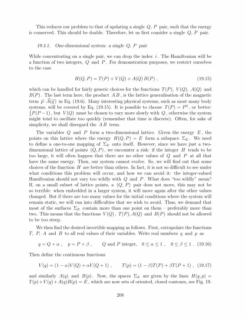
This reduces our problem to that of updating a single Q, P pair, such that the energyis conserved. This should be doable. Therefore, let us first consider a single Q, P pair.

19.4.1. One-dimensional system: a single Q, P pair

While concentrating on a single pair, we can drop the index i . The Hamiltonian will bea function of two integers, Q and P . For demonstration purposes, we restrict ourselvesto the case

H(Q,P ) = T (P ) + V (Q) + A(Q)B(P ) , (19.15)

which can be handled for fairly generic choices for the functions T (P ), V (Q), A(Q) andB(P ) . The last term here, the product AB , is the lattice generalisation of the magnetic

term ~p · ~A(~q ) in Eq. (19.6). Many interesting physical systems, such as most many bodysystems, will be covered by Eq. (19.15). It is possible to choose T (P ) = P 2 , or better:12P (P −1) , but V (Q) must be chosen to vary more slowly with Q , otherwise the system

might tend to oscillate too quickly (remember that time is discrete). Often, for sake ofsimplicity, we shall disregard the AB term.

The variables Q and P form a two-dimensional lattice. Given the energy E , thepoints on this lattice where the energy H(Q,P ) = E form a subspace ΣE . We needto define a one-to-one mapping of ΣE onto itself. However, since we have just a two-dimensional lattice of points (Q,P ) , we encounter a risk: if the integer H tends to betoo large, it will often happen that there are no other values of Q and P at all thathave the same energy. Then, our system cannot evolve. So, we will find out that somechoices of the function H are better than others. In fact, it is not so difficult to see underwhat conditions this problem will occur, and how we can avoid it: the integer-valuedHamiltonian should not vary too wildly with Q and P . What does “too wildly” mean?If, on a small subset of lattice points, a (Q, P ) pair does not move, this may not beso terrible: when embedded in a larger system, it will move again after the other valueschanged. But if there are too many values for the initial conditions where the system willremain static, we will run into difficulties that we wish to avoid. Thus, we demand thatmost of the surfaces ΣE contain more than one point on them – preferably more thantwo. This means that the functions V (Q) , T (P ), A(Q) and B(P ) should not be allowedto be too steep.

We then find the desired invertible mapping as follows. First, extrapolate the functionsT, P, A and B to all real values of their variables. Write real numbers q and p as

q = Q+ α , p = P + β , Q and P integer, 0 ≤ α ≤ 1 , 0 ≤ β ≤ 1 . (19.16)

Then define the continuous functions

V (q) = (1− α)V (Q) + αV (Q+ 1) , T (p) = (1− β)T (P ) + βT (P + 1) , (19.17)

and similarly A(q) and B(p) . Now, the spaces ΣE are given by the lines H(q, p) =T (p)+V (q)+A(q)B(p) = E , which are now sets of oriented, closed contours, see Fig. 19.

208

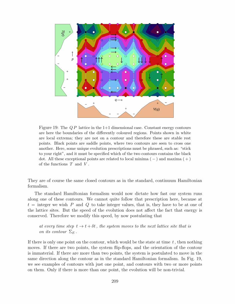
p

q

V(q)

T(p) +

+

+

+

+

+

−

−

−

−

−−−

−

Figure 19: The QP lattice in the 1+1 dimensional case. Constant energy contoursare here the boundaries of the differently coloured regions. Points shown in whiteare local extrema; they are not on a contour and therefore these are stable restpoints. Black points are saddle points, where two contours are seen to cross oneanother. Here, some unique evolution prescriptions must be phrased, such as: “stickto your right”, and it must be specified which of the two contours contains the blackdot. All these exceptional points are related to local minima (− ) and maxima ( + )of the functions T and V .

They are of course the same closed contours as in the standard, continuum Hamiltonianformalism.

The standard Hamiltonian formalism would now dictate how fast our system runsalong one of these contours. We cannot quite follow that prescription here, because att = integer we wish P and Q to take integer values, that is, they have to be at one ofthe lattice sites. But the speed of the evolution does not affect the fact that energy isconserved. Therefore we modify this speed, by now postulating that

at every time step t→ t+ δt , the system moves to the next lattice site that ison its contour ΣE .

If there is only one point on the contour, which would be the state at time t , then nothingmoves. If there are two points, the system flip-flops, and the orientation of the contouris immaterial. If there are more than two points, the system is postulated to move in thesame direction along the contour as in the standard Hamiltonian formalism. In Fig. 19,we see examples of contours with just one point, and contours with two or more pointson them. Only if there is more than one point, the evolution will be non-trivial.

209

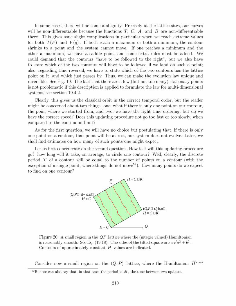
In some cases, there will be some ambiguity. Precisely at the lattice sites, our curveswill be non-differentiable because the functions T, C, A, and B are non-differentiablethere. This gives sone slight complications in particular when we reach extreme valuesfor both T (P ) and V (q) . If both reach a maximum or both a minimum, the contourshrinks to a point and the system cannot move. If one reaches a minimum and theother a maximum, we have a saddle point, and some extra rules must be added. Wecould demand that the contours “have to be followed to the right”, but we also haveto state which of the two contours will have to be followed if we land on such a point;also, regarding time reversal, we have to state which of the two contours has the latticepoint on it, and which just passes by. Thus, we can make the evolution law unique andreversible. See Fig. 19. The fact that there are a few (but not too many) stationary pointsis not problematic if this description is applied to formulate the law for multi-dimensionalsystems, see section 19.4.2.

Clearly, this gives us the classical orbit in the correct temporal order, but the readermight be concerned about two things: one, what if there is only one point on our contour,the point where we started from, and two, we have the right time ordering, but do wehave the correct speed? Does this updating procedure not go too fast or too slowly, whencompared to the continuum limit?

As for the first question, we will have no choice but postulating that, if there is onlyone point on a contour, that point will be at rest, our system does not evolve. Later, weshall find estimates on how many of such points one might expect.

Let us first concentrate on the second question. How fast will this updating procedurego? how long will it take, on average, to circle one contour? Well, clearly, the discreteperiod T of a contour will be equal to the number of points on a contour (with theexception of a single point, where things do not move52). How many points do we expectto find on one contour?

P

Q

(Q,P) = ε(b,a)

H = C

H = C

H = C + K

H = C + K

(Q,P) = ε(−a,b)

Figure 20: A small region in the QP lattice where the (integer valued) Hamiltonianis reasonably smooth. See Eq. (19.18). The sides of the tilted square are ε

√a2 + b2 .

Contours of approximately constant H values are indicated.

Consider now a small region on the (Q,P ) lattice, where the Hamiltonian H class

52But we can also say that, in that case, the period is δt , the time between two updates.

210

approximately linearises:

H class ≈ aP + bQ+ C , (19.18)

with small corrections that ensure that H class is an integer on all lattice points. With alittle bit of geometry, one finds a tilted square with sides of length ε

√a2 + b2 , where the

values of H class vary between values C and C+K , with K = ε(a2 +b2) . Assuming thatall these integers occur at about the same rate, we find that the total number of latticesites inside the square is ε2(a2 + b2) , and since there are K contours, every contour has,on average,

ε2(a2 + b2)/K = ε (19.19)

points on it. The lengths of the contours in Figure 20 is ε√a2 + b2 , so that, on average,

the distance between two points on a contour is√a2 + b2 .

This little calculation shows that, in the continuum limit, the propagation speed ofour updating procedure will be√(δq

δt

)2

+(δpδt

)2

=

√(∂H∂p

)2

+(∂H∂q

)2

, (19.20)

completely in accordance with the standard Hamilton equations! (Note that the factors2π in Eqs. (19.13) and (19.14) cancel out)

A deeper mathematical reason why our discrete lattice Hamiltonian formalism gen-erates the same evolution speed as the continuum theory may be traced to the Liouvilletheorem: a co-moving infinitesimal volume element in (p, q) -space stays constant in thecontinuum theory; in the discrete lattice case, time reversibility ensures that the numberof lattice points inside a small volume on the lattice stays fixed, so that we have the sameLiouville theorem on the lattice. When increasing values for the partial derivatives of theHamiltonian cause a squeezing of the infinitesimal volume elements, both the continuumtheory and the lattice theory require the same increase in the velocities to keep the volumeelements constant.

One concludes that our updating procedure exactly leads to the correct continuumlimit. However, the Hamiltonian must be sufficiently smooth so as to have more than onepoint on a contour. We now know that this must mean that the continuous motion inthe continuum limit cannot be allowed to be too rapid. We expect that, on the discretelattice, the distance between consecutive lattice points on a contour may vary erratically,so that the motion will continue with a variable speed. In the continuum limit, this mustaverage out to a smooth motion, completely in accordance with the standard Hamiltonequations.

Returning to the question of the contours with only one point on them, we expecttheir total lengths, on average, to be such that their classical periods would correspondto a single time unit δt . These periods will be too fast to monitor on our discrete timescale.

211

This completes our brief analysis of the 1+1 dimensional case. We found an evolutionlaw that exactly preserves the discrete energy function chosen. The procedure is unique assoon as the energy function can be extended naturally to a continuous function betweenthe lattice sites, as was realised in the case H = T +V +AB in Eq. (19.17). Furthermorewe must require that the energy function does not vary too steeply, so that most of theclosed contours contain more than one lattice point.

An interesting test case is the choice

T (P ) = 12P (P − 1) ; V (Q) = 1

2Q(Q− 1) , (19.21)

This is a discretised harmonic oscillator whose period is not exactly constant, but this oneis easier to generalise to higher dimensions than the oscillator described in section 17.2and subsection 19.3.1.

19.4.2. The multi dimensional case

A single particle in 1 space- and 1 time dimension, as described in the previous section,is rather boring, since the motion occurs on contours that all have rather short periods(indeed, in the harmonic oscillator, where both T and V are quadratic functions of theirvariables, such as in Eq. (19.21), the period will stay close to the fundamental time stepδt itself). In higher dimensions (and in multi component oscillators, particularly whenthey have non-linear interactions), this will be quite different. So now, we consider the

variables Qi, Pi, i = 1, · · · , n . Again, we postulate a Hamiltonian H( ~Q, ~P ) that, whenPi and Qi are integer, takes integer values only. Again, let us take the case that

H( ~Q, ~P ) = T (~P ) + V ( ~Q ) + A( ~Q )B(~P ) . (19.22)

To describe an energy conserving evolution law, we simply can apply the procedure de-scribed in the previous section n times for each cycle. For a unique description, it is nowmandatory that we introduce a cyclic ordering for the values 1, · · · , n that the index ican take. Naturally, we adopt the notation of the values for the index i to whateverordering might have been chosen:

1 < 2 < · · · < n < 1 · · · . (19.23)

We do emphasise that the procedure described next depends on this ordering.

Let Uopi be our notation for the operation in one dimension, acting on the variables

Qi, Pi at one given value for the index i . Thus, Uopi maps (Pi, Qi) 7→ (P ′i , Q

′i) using

the procedure of section 19.4.1 with the Hamiltonian (19.22), simply keeping all othervariables Qj, Pj, j 6= i fixed. By construction, Uop

i has an inverse Uop−1i . Now, it is

simple to produce a prescription for the evolution Uop for the entire system, for a singletime step δt = 1 :

Uop(δt) = Uopn Uop

n−1 · · · Uop1 . (19.24)

where we intend to use the physical notation: Uop1 acts first, then Uop

2 , etc., although theopposite order can also be taken. Note, that we have some parity violation: the operators

212

Uopi and Uop

j will not commute if i 6= j , and therefore, if n ≥ 3 , the resulting operatorUop is not quite the same as the one obtained when the order is reversed.

Time inversion gives:

Uop(−δt) = Uop−1(δt) = Uop−11 Uop−1

2 · · · Uop−1n . (19.25)

Finally, if the exchange Uopi ↔ Uop−1

i might be associated with “particle-antiparticleconjugation”, C , then the product P (parity) T (time inversion) C (conjugation) maystill be a good symmetry. In the real world, this might lead to a natural explanation ofCPT symmetry, while P , T , or CP are not respected.

19.4.3. The Lagrangian

It was emphasised by Elze [65] that systems with a discrete Hamiltonian should also havean action principle. If both time as well as the variables P and Q are discrete, one couldconsider Lagrangians such as

L(t)?= 1

2P (t)(Q(t+ 1)−Q(t− 1))−H(P (t), Q(t)) , S =

∑t∈Z

L(t) . (19.26)

This, however, would lead to Lagrange equations that are finite difference equations, atbest, while they would no longer guarantee conservation of energy. Some Lagrangians mayexist that are purely quadratic in the integers P and Q , but, as we saw, this would betoo strong a restriction that excludes any non-trivial theory. At this moment we have noproposal for a Lagrange principle that works as well as our discrete Hamilton formalism.

19.4.4. Discrete field theories

An important example of an infinite-dimensional (Qi, Pi) system is a local field theory.Suppose that the index i is replaced by a lattice coordinate ~x , plus possibly other indicesj labelling species of fields. Let us rename the variables (Φj(~x ), Pj(~x )) , where Φj arecanonical fields and Pj are their momentum variables (often, in the continuum theory,ddt

Φj ). Now assume that the Hamiltonian of the entire system is the sum of local terms:

H int =∑~x

H int(~x ) , H int(~x ) = V (~Φ(~x ), ~Φ(~x ′)) + T (~P (~x )) , (19.27)

where the coordinates ~x ′ are limited to neighbours of ~x only, and all functions V andT are integers. This would be a typical discretisation of a (classical or quantum) fieldtheory (ignoring, for simplicity, magnetic terms).

We can apply our multi-dimensional, discrete Hamiltonian equations to this case, butthere is one important thing to remember: where in the previous subsections we statedthat the indices i must be cyclically ordered, this now means that, in the field theory ofEq. (19.27), not only the indices i but also the coordinates ~x must be (cyclically) ordered.The danger of this is that the functions Vi(~x ) also refer to neighbours, and, consequently,

213

the evolution step defined at point ~x affects the evolution at its neighbouring points ~x ′ ,or: [Uop(~x ), Uop(~x ′ )] 6= 0 . Performing the updates in the order of the values of thecoordinates ~x , might therefore produce signals that move much faster than light, possiblygenerating instantaneous non local effects across the entire system over a single time stept→ t+ δt . This we need to avoid, and there happens to be an easy way to do this:

First make sure that the interaction terms in the Hamiltonian only involvenearest neighbours, The evolution equations (e.o.m.) of the entire systemover one time step δt , are then obtained by ordering the coordinates andother indices as follows: first update all even lattice sites, then update all oddlattice sites.

Since the Uop operators generated by Hi(~x ) do commute with the evolution operatorsUop(~x ′ ) when ~x and ~x ′ are both on an even site or both on an odd site of the lattice (sothat they are not nearest neighbours), this ordering does not pass on signals beyond twolattice links. Moreover, there is another huge advantage of this law: the order in whichthe individual even sites of the lattice are updated is now immaterial, and the same forthe set of all odd sites.

Thus, we obtained a cellular automaton whose evolution law is of the type

Uop = AopBop , Aop =∏

~x= even

Aop(~x) , Bop =∏

~y= odd

Bop(~y) , (19.28)

where the order inside the products over the sites ~x and ~y is immaterial, except thatAop(~x) and Bop(~y) do not commute when ~x and ~y are direct neighbours. Such automataare interesting objects to be studied, see chapter 21.

19.4.5. From the integer valued to the quantum Hamiltonian

A deterministic system obeying a discrete Hamiltonian formalism as described in theprevious sections is of particular interest when we map it onto a quantum system followingthe program discussed in this book. This is because we here have two different operatorsthat both play the role of energy: we have the integer valued, discrete Hamiltonian H class

that generates the classical equations of motion, and we have the angular, or fractionalvalued Hamiltonian H quant , defined from the eigenstates and eigenvalues of the one-timestep evolution operator Uop(δt) :

Uop(δt) = e−iHopquant , 0 ≤ H quant < 2π (δt = 1) , (19.29)

where H quant refers to the eigenvalues of the operator Hopquant .

As anticipated in section 19.4, we can now uniquely define a total Hamiltonian thatis a real number operator, by

H = H class +Hopquant . (19.30)

214

The bounds imposed in Eq. (19.29) are important to keep in mind, since H quant , asdefined, is strictly periodic. H class is assumed to take only integer values, times 2π/δt .In this section we study the quantum theory defined by the Hamiltonian (19.30).

We have seen, for instance in chapter 2, subsection 2.2.1, Eq. 2.26 in part I, and inchapter 12, section 12.2, Eq. 12.10 in part II, how the operator Hop

quant can be calculatedfrom the eigenvalues U(δt) of the operator Uop(δt) : for instance by Fourier transforma-tions, one derives that, if the eigenvalues of H quant are assumed to lie between 0 and 2π ,then

Hopquant = π −

∞∑n−1

i

n(Uop(n δt)− Uop(−n δt) ) . (19.31)

This sum converges nearly everywhere, but the vacuum is the edge state where the equa-tion does not hold, and it is not quite local, since the evolution operator over n steps intime, also acts over n steps in space.

But both H class and H quant are uniquely defined, and since H quant is bound to aninterval while H class is bounded from below, also H is bounded from below.

Note that demanding a large number of low energy states near the vacuum (the absenceof a large mass gap) implies that Uop(n δt) be non-trivial in the H class = 0 sector. Thisis often not the case in the models described in subsection 19.4.2, but in principle there isno reason why such models should not exist also. In fact, some of the cellular automatonmodels discussed later in chapter 21 have no manifestly conserved H class , so that all theirstates can be regarded as sitting in the H class = 0 sector of the theory.

Because of the non-locality of Eq. (19.31), the Hamiltonian (19.31) does not obey therule vi , but if Uop(δt) is the product of local evolution operators, the evolution overinteger time steps n δt is local, so the theory can be claimed to obey locality, as long aswe refrain from defining its states at time t when t is not an integer.53

As we have seen in section 14, the sum (19.31) does not converge rapidly everywherein Hilbert space. We are particularly interested in the Hamiltonian as it acts on statesvery close to the vacuum, in our notation: H class = 0, H quant = ω , where 0 < ω 2π .Suppose then that we introduce a cut-off in the sum (19.31) (or 12.8) by multiplying thesummand with e−n/R , where R is also the range of non-locality of the last significantterms of the sum. As we have seen in section 14, breaking off the expansion at the pointR modifies the Hamiltonian as follows:

H quant → H quant +2

RH quant

, (19.32)

and this is only acceptable if

RMPl/〈H quant〉2 . (19.33)

53Some have tried to shoot down our theories by objecting that our classical/quantum equivalence onlyholds for integer times. Of course we simply point out then that, if we restrict ourselves to sufficientlylow energies, the time-variability is sufficiently slow that having an equation that only holds rigorouslyat integer multiples of δt is all we need.

215

Here, MPl is the “Planck mass”, or whatever the inverse is of the elementary time scalein the model. This cut-off radius R must therefore be chosen to be very large, so that,indeed, the exact quantum description of our local model generates non-locality in theHamiltonian.

We conclude that the Hamiltonian can be expressed in terms of local terms, but weneed to include the operators Uop(±∆t) where ∆t is large compared to the inverse of theHamiltonian we wish to calculate. These will develop non localities that are still serious.This is still an obstacle against the construction of a local quantum Hamiltonian density(the classical component, H class obeys condition vi). As yet, therefore, more has to bedone to obtain locality: second quantisation.

The apparent locality clash between the quantum Hamiltonian and the classical theorymay well be looked upon as a possible additional explanation of the apparent non-localitiesexpected in ‘hidden variable’ theories: neither the pure quantum system that we usuallyemploy in quantum field theories, nor the associated classical system exhibit any non-locality, but the mapping between them does. This non-locality is spurious, it has nophysical consequence whatsoever, but mathematically it may imply that the quantumsystem should not be split up into local wave functions that do not communicate witheach other – perhaps that is the route along which apparent non-locality arises in classicalmechanical models. There is no non-locality in the classical theory, but it is in therepresentation of the quantum variables, or: the classical - quantum mapping.

20. Quantum Field Theory

In this chapter, we give a brief summary of the features of quantum field theory that weshall need to understand in this book.

We have seen that producing quantum Schrodinger equations starting from non quan-tum mechanical systems is essentially straightforward. However, to employ this observa-tion as a viable ontological interpretation of quantum mechanics, more is needed. Themain objection against these concepts has always been that quantum theories obeyinglocality in the quantum sense, are much more difficult to reproduce with classical systemsobeying locality in the classical sense, and impossible according to many.

Locality means that interaction at a distance can only occur with signals that undergosome delay. Locality in the classical sense here means that the classical evolution laws arebased on interactions with neighbouring sites only, in such a way that information cannotspread faster than the speed of light. Locality in the quantum sense means the samething, except that we allow for any kind of quantum mechanical interactions betweenneighbouring sites. If Oi(x) is an operator only depending on fundamental variables inthe immediate vicinity of a space-time point x , enumerated by an index i , then quantumlocality means that the commutation property

[Oi(x), Oj(x′)] = 0 , (20.1)

216

holds as soon as the two space-time points x and x′ are space-like separated:

(x− x′)2 ≡ (~x− ~x ′)2 − c2(t− t′)2 > 0 . (20.2)

The relativistic quantised field theories employed in the Standard Model are indeedstrictly local in the quantum mechanical sense, obeying Eqs. (20.1), (20.2). It is importantto recall here the essential features of these systems. A point to be made right-away is,that quantum field theories are quite complicated. This is partly due to the fact that weusually want special relativity to be valid, which is a difficult – while highly interesting– demand. But even without special relativity, there are some fairly intricate issues suchas second quantisation, perturbation theory, infinities, renormalisation, symmetries andanomalies. This is why the topic of this book is actually quite difficult: not only arewe attempting to derive quantum mechanics from scratch, but also (fully renormalised)quantum field theory.

Relativistic quantum field theories with a proper continuum limit can only incorporateelementary fields with spin 0, 1

2and 1. As is well-known, gravity would be propagated

by gravitons with spin 2, and supergravity would add one or more gravitino species withspin 3/2 , but then, if we want these fields to interact, we would have to be close to thePlanck scale, and this would require discretisation due to micro states. Since ordinaryquantum field theories assume strict continuity, they only apply to the continuum limit,which implies that we can safely omit spin 2 and spin 3/2 fields in those theories. Theway this works in quantum field theory is that, at the Standard Model scales, interactionswith gravitons and gravitinos are extremely weak.

On the other hand, one could argue that also special relativity is not our first priority,and ignoring special relativity would imply no rigorous constraint on spin. If we ignorespecial as well as general relativity, we could just as well ignore rotation invariance54.What is left then is a theory of quantised fields enumerated by an index that may or maynot represent spin. Later we may wish to reinstate Poincare invariance, at least at thequantum side of the equation, but this will have to be left as an important exercise forthe (hopefully near) future.

What we want to keep is a speed limit for signals that describe interactions, so thatthe notion of locality can be addressed. In practice, an elegant criterion can be given thatguarantees this kind of locality. Consider the quantum system in its Heisenberg notation.We have operators Oi(~x, t) where both the space coordinates ~x and the time coordinatet may be either continuous or discrete. The discrete index i enumerates different typesof operators.

When our operator fields obey quantum locality, Eqs. (20.1) and (20.2), in the con-tinuous case, this means that the Hamiltonian must be the integral of a Hamiltonian

54Ignoring such important symmetries in considering certain models does not mean that we believe thesesymmetries to be violated, but rather that we wish to focus on simple models where these symmetriesdo not, or not yet, play a role. In more sophisticated theories of Nature, of course one has to obey allknown symmetry requirements.

217

density:

H =

∫d3~x H(~x, t) , [H(~x, t) , H(~x ′, t)] = 0 if ~x 6= ~x ′ , (20.3)

while, when x → x′ , the commutator [H(~x, t) , H(~x ′, t) ] , may contain derivatives ofDirac delta distributions. Note that, here, we kept equal times t so that these space-timepoints are space-like separated unless they coincide.

On a discrete space-like lattice, it is tempting to replace Eqs. (20.3) by the latticeexpressions

H =∑~x

H(~x, t) , [H(~x,′ , t), H(~x ′, t)] = 0 if |~x− ~x ′| > a, (20.4)

where a is the link size of the lattice. The Hamiltonian densities at neighbouring sites,|~x− ~x ′| = a , will, in general, not commute. Although Eqs. (20.4) may well serve as agood definition of locality, they do not guarantee that signals are subject to a speed limit.Only in the continuum limit, one may recover commutation at space-like separations,(20.2), if special relativity holds (in that limit).

Cellular automata are typically lattice theories. In general, these theories are difficultto reconcile with Lorentz invariance. This does not mean that we plan to give up Lorentzinvariance; quite possibly, this important symmetry will be recovered at some stage. Butsince we want to understand quantum mechanics as a reflection of discreteness at a scalecomparable to the Planck scale, we are unable at present to keep Lorentz invariance inour models, so this price is paid, hopefully temporarily.

For simplicity, let us now return our attention to continuum quantum field theories,which we can either force to be Lorentz invariant, or replace by lattice versions at somelater stage. The present chapter is included here just to emphasise some important fea-tures.

20.1. General continuum theories – the bosonic case

Let the field variables be real number operators Φi(~x, t) and their canonical conjugatesPi(~x, t) . Here, i is a discrete index counting independent fields. The commutation rulesare postulated to be

[Φi(~x, t), Φj(~x′, t)] = [Pi(~x, t), Pj(~x

′, t)] = 0 ,

[Φi(~x, t), Pj(~x′, t)] = i δij δ

3(~x− ~x ′) (20.5)

(for simplicity, space was taken to be 3-dimensional).

In bosonic theories, when writing the Hamiltonian as

H =

∫d~xH(~x) , (20.6)

218

the Hamiltonian density H(~x) typically takes a form such as

H(~x) =∑i

(12P 2i (~x) + 1

2(~∂Φi(~x))2 + V (~Φ(~x))

). (20.7)

If we are in 3+1 dimensions, and we want the theory to be renormalizable, V (~Φ(~x)) must

be a polynomial function of ~Φ , of degree 4 or lower. Typically, one starts with

V (~Φ) = 12

∑i

m2i~Φ2i + V4(~Φ) , (20.8)

where mi are the (unrenormalized) masses of the particles of type i , and V4 is a homo-

geneous quartic expression in the fields ~Φi(~x) such as a self interaction 14!λΦ4 .

However, when ~Φ(~x) contains components that form a vector in 3-space, Lorentz-invariance dictates a deviation from Eq. (20.7). We then have local gauge invariance,

which implies that a constraint has to be imposed. Writing these vector fields as ~A(~x) ,

and their associated momentum fields as ~E(~x) , one is forced to include a time componentA0(~x) .

Gauge-invariance must then be invoked to ensure that locality and unitarity of thetheory are not lost, but the resulting Hamiltonian deviates a bit from Eq. (20.7). Thisdeviation is minimal if we choose the space-like radiation gauge

3∑i=1

∂iAi(~x) = 0 , (20.9)

since then the Hamiltonian will have the quadratic terms

H2(~x) = 12~E2(~x) + 1

2(~∂Ai(~x))2 − 1

2(~∂A0(~x))2 . (20.10)

In addition, one might have linear terms,

HJ(~x) = ~J(~x) · ~A(~x) + %(~x)A0(~x) , H ≡ H2 +HJ +H int , (20.11)

where ~J and % are some given background functions. ~J(~x) is a current density and %(~x)

a charge density. In a relativistic theory, ~J and % form a 4-vector. All remaining termsin the Hamiltonian, typically higher powers of the fields, which may cause interactionsamong particles to occur, are collected in H int .

Notably, the field A0(~x) does not have a canonical partner that would have beencalled E0(~x) , and therefore, the field A0 can be eliminated classically, by extremisingthe Hamiltonian H =

∫d~xH(~x) , which leads to the Coulomb force between the sources

% . This Coulomb force is instantaneous in time, and would have destroyed locality (andhence Lorentz invariance) if we did not have local gauge invariance.

This, of course, is a description of quantised field theories in a nut shell, as yet only forbosonic particles. How then the Schrodinger equation is solved by perturbation expansion

219

in powers of the coupling constant(s) λ and/or gauge coupling parameters g , is well-known and discussed in the standard text books. [29][66][83]

The most important point we need to emphasise is that the above formulation ofquantised field theories is easy to replace by discretised versions. All we need to do isreplace the partial derivatives ∂i = ∂/∂xi by lattice derivatives:

∂iΦ(~x)→ 1

a

(Φ(~x+ ~eia)− Φ(~x)

), (20.12)

where a is the lattice link size, and ~ei is the unit vector along a lattice link in the idirection. The continuum limit, a ↓ 0 , seems to be deceptively easy to take; in partic-ular, renormalization will now only lead to finite correction terms. Note however, thatsymmetries such as rotation symmetry and Lorentz invariance will be lost. Recoveringsuch symmetries in more sophisticated models (without taking a continuum limit) is be-yond our abilities just now – but notice that our treatment of string theory, section 17.3,appears to be heading in the right direction.

20.2. Fermionic field theories

Fermionic field systems are also an essential element in the Standard Model. The funda-mental variables are the Dirac fields ψi(~x) and their canonical associates ψ†i (~x) . Theyare spinor fields, so that i contains a spinor index. The fields anti -commute. The anti-commutation rules are

ψ†i (~x), ψj(~x′) = δijδ(~x− ~x ′) , ψi, ψj = ψ†i , ψ

†j = 0 , (20.13)

where a, b ≡ ab+ ba . Note, that these rules are typical for operators of the form (0 10 0

)

and (0 01 0

) , so these rules mean that ψi(~x) is to be regarded as an operator that annihilates

an object i at position ~x , and ψ†i (~x) creates one. The rules imply that ψ2i (~x) = 0 and

(ψ†i (~x))2 = 0 , so that we cannot create or annihilate two objects i at the same spot ~x .A state containing two (or more) particles of different type, and/or at different positions~x , will always be antisymmetric under interchange of two such fermions, which is Pauli’sprinciple.

In conventional quantum field theory, one now proceeds to the Lagrange formalism,which works magnificently for doing fast calculations of all sorts. For our purpose, how-ever, we need the Hamiltonian. The quantum Hamiltonian density for a fermionic fieldtheory is (compare section 15.2):

HF (~x) = ψ (m+W (~Φ) + ~γ · ~∂)ψ , (20.14)

where W (~Φ) stands short for the Yukawa interaction terms that we may expect, andψ = ψ†γ4 .

The matrices γµ, µ = 1, 2, 3, 4 , need to obey the usual anti-commutation rule

γµ, γν = 2δµν , (20.15)

220

which requires them to be at least 4× 4 matrices, so that the spinors are 4 dimensional.One can, however, reduce these to 2 component spinors, called Majorana spinors, by usinga constraint such as

ψ = C ψ = Cγ4ψ† , ψ† = C∗γ4 ψ , (20.16)

where ˜ stands for transposition, and C is a spinor matrix obeying 55, 56

γµC = −Cγ∗µ , C†C = 1 , C = C† . (20.17)

Just as in the bosonic case, we may consider replacing the continuum in space by aspace-like lattice, using expressions such as Eq. (20.12), at the price of (hopefully tem-porarily) giving up Lorentz invariance.

The Yukawa term W (Φ) in Eq. (20.14) may include interactions with gauge fields inthe usual way. The question addressed in this work is to what extent Hamiltonians suchas the sum of Eqs. (20.7) and (20.14) can be obtained from deterministic theories.

20.3. Standard second quantisation

Accurate calculations in field theories for interacting particles are practically impossiblewithout a systematic approximation procedure of some sort. The most efficient approx-imation scheme used is that of the perturbation expansion in terms of powers of allinteraction parameters. This works because, when the interaction terms vanish, the fieldswill obey linear field equations, which are trivial to solve.

These linear equations happen to coincide with the linear Schrodinger equations obeyedby single particle states. It is as if the wave functions |φi(~x, t)〉, |ψi(~x, t)〉 and theirassociated bra states are replaced by classical ontological fields Φi(~x, t), ψi(~x, t) and theircanonical conjugates, after which the quantisation procedure is applied to these fields yetagain, replacing Poisson brackets by commutators or anticommutators. This explains theterm “second quantisation” by which this procedure is known.

In fact it is not hard to show that the complete Hilbert space of all quantum states ofthe quantised field system (20.5) and (20.13) can be described as the product space of allsets of multi particle states that can be formed out of the ‘single-quantised’ particles.

Then, however, one has to insert the interaction terms of the Hamiltonian. We write

H = H0 + ∆H0 +H int + ∆H int , (20.18)

where H0 = H2 + HJ is the bilinear part of H , and H int contains the higher powersof the fields, causing interactions. ∆H0 and ∆H int are extra terms that are of the

55In section 15.2, we also used 2 dimensional spinors. The two-component spinor field used thereis obtained by using one of the projection operators P± = 1

2 (1 ± γ5) . The mass term can be madecompatible with that.

56The reason why Dirac needed a four-dimensional representation is that the constraint (20.16) wouldnot allow coupling to an electromagnetic field since this would violate gauge-invariance (in particular themass term).

221

same form as H0 and H int themselves, but they are taken care of at later stages ofthe perturbation expansion, just for technical reasons (renormalization). This is how onebegins to set up perturbation theory.

Now, in relativistic quantum theories, the single-quantised free particles have energyspectra that take the form E = ±

√p2 +m2 (for bosons), or E = ~α · ~p + β m (for

fermions; αi and β are the Dirac matrices). This implies that the energies of singleparticles appear to be unbounded from below. The beauty of the second-quantised theoryis that we can replace negative-energy particles by holes of positive energy antiparticles.This automatically ensures a lower bound for the total Hamiltonian.

For the case of fermions, it is easy to accept the idea that negative energy particleshave to be regarded as holes in the sea of antiparticles, because Pauli’s exclusion prin-ciple forbids the presence of more than one particle in any energy level. In the case ofbosons, the situation becomes clear if we regard every mode of the energy spectrum as aharmonic oscillator, controlled by creation and annihilation operators. Its energy is alsobounded from below. Note that, in terms of the quantum field variables Φ and ψ , theHamiltonian was non-negative by construction – if one disregards the complications dueto renormalization.

Thus, the second quantisation procedure restores a lower bound to the Hamiltonian,simply by allowing indefinite numbers of particles. We can allow the same mechanism towork for a cellular automaton, if the automaton also can be described in terms of particles.A particle hops over a grid of points in 3-space, and its evolution operator generates aHamiltonian that may be unbounded from below. Second quantisation now means thatwe allow for the presence of indefinite numbers of these particles, which may either behaveas fermions or as bosons. The particle - antiparticle procedure then ensures positivity ofthe total Hamiltonian.

20.4. Perturbation theory

How to compute the effects of these Hamiltonians in perturbation theory, such as massspectra, cross sections and lifetimes of the quantised particles that it contains, is standardtext material, and not the subject of this treatise, but we do need to know about someessential features for our further discussion.

Split up the Hamiltonian into a “free” part H0 and the various interaction parts, as inEq. (20.18), where the free part only contains terms that are bilinear in the field variablesΦi(~x), Pi(~x), ψi(~x) and ψi(~x) (possibly after having shifted some of the fields by a vac-uum value, such as in the Brout-Englert-Higgs mechanism). The interaction HamiltonianH int may also contain bilinear terms, here written as ∆H0 , needed to renormalize di-vergent effective interactions. There is some freedom as to whether we put parts of theseso-called counter terms in H0 or in ∆H0 , and how to split the interaction terms in H int

and ∆H int , which in fact is a choice concerning the book keeping process of the pertur-bative expansion. The fact that final results of the calculation should be independent ofthese choices is an important ingredient of what is called the renormalization group of thetheory (see section 20.8).

222

H int is assumed to depend on the coupling parameters λi, gi, etc., of the theory,such that H int vanishes if these parameters are set to zero.

As already mentioned in section 20.1, the analysis is facilitated by the introduction ofauxiliary terms in the Hamiltonian, called source terms, which are linear in the fields:

HJ(~x, t) =∑i

Ji(~x, t)Φi(~x) +∑i

ηi(~x, t)ψi(~x) +∑i

ψi(~x)ηi(~x, t) , (20.19)

where the “source functions” Ji(~x, t), ηi(~x, t) and ηi(~x, t) are freely chosen functions ofspace and time, to be replaced by zero at the end of the computation (the time dependenceis not explicitly mentioned here in the field variables, but, in a Heisenberg representation,of course also the fields are time dependent).

These source terms could serve as simple models for the creation of the initial particlesin a scattering experiment, as well as the detection process for the particles in the finalstate, but they can also simply be regarded as useful devices for a mathematical analysis ofthe physical properties of the system. One can then find all amplitudes one needs to know,by computing at any desired order in perturbation theory, that is, up to certain powersof the coupling parameters and the source functions, the vacuum-to-vacuum amplitude:

t=∞〈 ∅ | ∅ 〉t=−∞ = 1− i2

∫ ∫d4xd4x′ Ji(x)Jj(x

′)Pij(x− x′) +16

∫ ∫ ∫d4xd4x′d4x′′Wijk(x, x

′, x′′)Ji(x)Jj(x′)Jk(x

′′) + · · · , (20.20)

where x stands short for the space-time coordinates (~x, t) , and the correlation functionsPij(x − x′), Wijk(x, x

′, x′′) and many more terms of the sequence are to be calculated.Physically, this means that we compute expectation values of the products of operatorsΦi(~x, t), ψi(~x, t) and ψi(~x, t) of Eq. (20.19) in a Heisenberg representation. Local prod-ucts of these operators also follow from the expressions (20.20), if we take space-timepoints x and x′ to coincide.

The algorithm for the calculation of the two-point functions P , the three-point func-tions W , etc., is conveniently summarised in the so-called Feynman rules, for which werefer to the standard text books. [36][66][83]

20.4.1. Non-convergence of the coupling constant expansion

There are some conditions where particles interact strongly. Quarks are fermionic particlesthat interact so strongly that the forces between them keep them permanently bound inhadrons, the so-called quark confinement mechanism. This, however, only happens atthe distance scale of the Standard Model, When extrapolated to the Planck scale, thesestrong interactions have been calculated to be about as weak as the other forces, notablyelectromagnetism and the weak force. This means that, in a conveniently large domainnear the Planck scale, all perturbation expansions may be rapidly convergent: there, onenever needs to know the very high-order perturbative correction terms, since these aremany times smaller than the usual margins of error in our description of the dynamics.

It now so happens that, when we apply second quantisation in our cellular automatonmodels, something very similar may happen. If we choose our interactions to originate

223

from rare coincidences in the cellular configurations, then most of the interaction eventsmay be far separated at the Planck scale. This may imply that we have freely movingparticles interacting only weakly by means of an interaction Hamiltonian. Since thisHamiltonian starts out to be local, only a few higher order calculations may suffice toobtain an accurate description of the dynamics.

We can now consider combining the quantum field theoretic perturbation expansionwith the expansion needed to generate the interaction Hamiltonian itself. The result-ing theory will still be accurate in the domain close to the Planck scale. Our proposalis to start from this theory, and to apply the usual renormalization group procedures(section 20.8) to transform everything to the Standard Model scale.

20.5. The algebraic structure of the general, renormalizable, relativisticquantum field theory

The reasons for limiting ourselves to renormalizable quantum field theories are not com-pletely obvious. When coupling strengths become large, renormalizable field theories maygenerate poles where the perturbation expansion diverges. We call these Landau poles.Renormalization is then of little help. The renormalization group (section 20.8) explainshow the Landau poles can arise. If a Landau pole emerges in the small-distance domain,one has to conclude that the renormalization procedure fails, and here is little one can doabout this. If however a Landau pole is related to a large distance divergence, it can beattributed to non-canonical behaviour of the force fields at large distances, which can beinvestigated and understood.

Landau poles do also occur when the couplings are weak, but since they are non-perturbative effects, these poles retreat to very distant domains of extremely high energies,so that they quickly turn harmless. This is the case where, by demanding renormalizabil-ity, we can select out a precisely defined class of models that are mathematically accurate,and most useful for comparison with experiments. They are not infinitely accurate, but,as we shall see in section 22.1, also the procedure that we can use to derive a field theoryout of a cellular automaton, will have an accuracy that appears to be limited by theinteraction strength.

Finally, we note that, indeed, in the Standard Model itself, the interaction parametersare remarkably small. This was not known or expected to be the case, a few decades ago.

Relativistically invariant, renormalizable quantum field theories have a remarkablyrich mathematical structure. There are vector fields (for elementary particles with spin1), spinor fields (fermions with spin 1/2 ), and scalars (spin 0).

The vector fields have to be associated with a local gauge theory, usually of the Yang-Mills type. The number of distinct vector particle species equals the number of dimensions,also called the rank, of the local gauge group. Electromagnetism has U(1) as its localgauge group; the dimension is 1, so there is one photon species.The electro-weak interactions have this local gauge theory enlarged to U(1) ⊗ SU(2) ,with group dimension 4, while the strong force adds to this SU(3) , with dimension 8.

224

The fermionic and the scalar fields must all come as representations of the gaugegroup. They each transform trivially or non-trivially under local gauge transformations.This determines how these particles couple to the vectorial gauge fields.

The fermions are based on Dirac’s field equation, and the scalars start off with theKlein-Gordon equation. The interactions between these fields are written as Yukawaterms for the fermions, and quartic, sometimes also cubic, self interactions for the scalars.The allowed couplings are severely constrained by the condition that the system has tobe renormalizable and gauge-invariant.

After all algebraic equations have been written down, it must be checked explicitlywhether there are chiral anomalies. These are clashes between current-conservation lawsin the chiral symmetries one might expect in the theory. Anomalies that would be harm-ful for the self consistency of the theory only occur when right-handed fermions coupledifferently to the gauge fields than left handed ones. One then has to see to it that theseanomalies cancel out. They indeed do in the Standard Model.

In the Standard Model, the algebra turns out to be arranged in such a way that thefermions come as three identical copies (“generations”) of quarks and leptons. Quarkscome as triplet representations of the gauge SU(3) group, while the leptons are SU(3)singlets. All fermions couple, at least to some extent, to the SU(2)⊗ U(1) gauge fields,with the exceptions of the right-handed components of the neutrinos, which do not coupleto the gauge fields at all.

In principle, however, the mathematical rules known today would have allowed justany compact Lie group as the gauge group, and any kinds of representations for thefermions and the scalars, as long as there are not too many of those.

This summary here illustrates that the mathematical structure of the generic quantumfield theory, and the Standard Model in particular, is fairly complex. It would have tobe reproduced in a deterministic theory of nature. Further details are to be found innumerous text books. See for instance [29], [36].

20.6. Vacuum fluctuations, correlations and commutators

Because all contributions to our Hamiltonian are translation invariant, one expects thecorrelation functions to be translation invariant as well, and this is a good reason toconsider their Fourier transforms, so, instead of x space, one considers k space:

Pij(x(1) − x(2)) = (2π)−4

∫d4kPij(k) eik(x(1)−x(2)) , (20.21)

where we will often omit the caret ( ).

Disregarding factors 2π for the moment, one finds that the two-point functions arebuilt from elementary expressions such as the Feynman propagator,

∆Fm(x) ≡ −i

∫d4k

eikx

k2 +m2 − iε,

x = x(1) − x(2) , k2 = ~k2 − k20 , (20.22)

225

where ε is an infinitesimal positive number, indicating how one is allowed to arrangethe complex contour when k0 is allowed to be complex. This propagator describes thecontribution of a single, non interacting particle to the two-point correlation function. Ifthere are interactions, one finds that, quite generally, the two-point correlation functionstake the form of a dressed propagator :

∆F (x) =

∫ ∞0

dm%(m) ∆Fm(x) , (20.23)

where %(m) is only defined for m ≥ 0 and it is always non-negative. This property isdictated by unitarity and positivity of the energy, and always holds exactly in a relativisticquantum field theory [83]. The function %(m) can be regarded as the probability that anintermediate state emerges whose centre-of-mass energy is given by the number m . Inturn, %(m) can be computed in terms of Feynman diagrams with two external legs; itdescribes what may happen to a virtual particle as it travels from x(2) to x(1) . Diagramswith more external legs (which are usually the contributions to the scattering matrix withgiven numbers of free particles asymptotically far away in the in-state and the out-state),can be computed with these elementary functions as building blocks.

The two-point function physically corresponds to the vacuum expectation value of atime-ordered product of operators:

Pij(x(1) − x(2)) = 〈 ∅ |T (Φi(x

(1)),Φj(x(2))| ∅ 〉 , (20.24)

where

T (A(t1), B(t2)) = A(t1)B(t2) , if t1 > t2 ,

= B(t2)A(t1) , if t2 > t1 (20.25)

(for fermions, this is to be replaced by the P product: a minus sign is added if twofermions are interchanged).

We shall now show how, in explicit calculations, it is always found that two operatorsO1(x(1)) and O2(x(2)) commute when they both are local functions of the fields Fi(~x, t) ,and when their space-time points are space-like separated:

(~x )2 − (x0)2 > 0 , x = x(1) − x(2) . (20.26)

To this end, one introduces the on-shell propagators :

∆±m(x) = 2π

∫d4k eikx δ(k2 +m2)θ(±k0) ; k x = ~k · ~x− k0x0 . (20.27)

By contour integration, one easily derives:

∆Fm(x) = ∆+

m(x) if x0 > 0 ;

= ∆−m(x) = ∆+m(−x) if x0 < 0 ;

∆F∗m (x) = ∆−m(x) if x0 > 0 ;

= ∆+m(x) if x0 < 0 . (20.28)

226

Here, ∆F∗m is obtained from the Feynman propagator DF

m in Eq. (20.22) by replacing iwith −i .

Now we can use the fact that the expressions for ∆Fm(x) and ∆±m(x) are Lorentz-

invariant. Therefore, if x is space-like, one can always go to a Lorentz frame wherex0 > 0 or a Lorentz frame where x0 < 0 , so then,

∆Fm(x) = ∆+

m(x) = ∆−m(x) = ∆F∗m (x) = ∆F

m(−x) . (20.29)

This implies that, in Eq. (20.24), we can always change the order of the two operatorsO(x(1)) and O(x(2)) if x(1) and x(2) are space-like separated. Indeed, for all two-pointfunctions, one can derive from unitarity that they can be described by a dressed propagatorof the form (20.23), where, due to Lorentz invariance, %(m) cannot depend on the signof x0 . The only condition needed in this argument is that the operator O1(x(1)) is alocal function of the fields Φi(x

(1)) , and the same for O2(x(2)) . To prove that compositefields have two-point functions of the form (20.23), using unitarity and positivity of theHamiltonian, we refer to the literature [66]. To see that Eqs. (20.29) indeed imply thatcommutators between space-like separated operators vanish, and that this implies the nonexistence of information carrying signals between such points, we refer to section 20.7.

Now it is crucial to notice that the Feynman propagator ∆Fm(x) itself does not vanish

at space-like separations. In general, one finds for free fields with mass m , at vanishingx(1)0 − x(2)0 , and writing ~r = ~x(1) − ~x(2) ,

〈 ∅ |T (Φ(x(1)), Φ(x(2)) | ∅ 〉 = (2π)−4∆Fm(0, ~r ) =

∫d3~k

1

2(2π)3√~k2 +m2

ei~k·~r

=1

(2π)2

∫ ∞0

k2

√k2 +m2

eik|~r | , (20.30)

but, since the fields here commute, we can omit the T symbol. When the productm |~r| becomes large, this vanishes rapidly. But when m vanishes, we have long-rangecorrelations:

〈 ∅ |Φ(0, ~r) Φ(0,~0 ) | ∅ 〉 =1

(2π)2 ~r 2. (20.31)

For instance, for the photon field, the vacuum correlation function for the two-pointfunction is, in the Feynman gauge,

〈 ∅ |Aµ(0, ~r)Aν(0,~0 ) | ∅ 〉 =gµν

(2π)2 ~r 2. (20.32)

This means that we do have correlations over space-like distances. We attribute thisto the fact that we always do physics with states that are very close to the vacuum state.The correlations are non-vanishing in the vacuum, and in all states close to the vacuum(such as all n -particle states, with n finite). One may imagine that, at very high orinfinite temperature, all quantum states will contribute with equal probabilities to theintermediate states, and this may wipe out the correlations, but today’s physics always

227

stays restricted to temperatures that are very low compared to the Planck scale, most ofthe time, at most places in the Universe.

There is even more one can say. Due to the special analytic structure of the propagators∆Fm(x) , the n point functions can be analytically continued from Minkowski space-time

to Euclidean space-time and back. This means that, if the Euclidean correlation functionsare known, also the scattering matrix elements in Minkowski space-time follow, so that theentire evolution process at a given initial state can be derived if the space like correlationfunctions are known. Therefore, if someone thinks there is “conspiracy” in the space-likecorrelations that leads to peculiar phenomena later or earlier in time, then this mightbe explained in terms of the fundamental mathematical structure of a quantum fieldtheory. The author suspects that this explains why “conspiracy” in “unlikely” space-likecorrelations seems to invalidate the Bell and CHSH inequalities, while in fact this may beseen as a natural phenomenon. In any case, it should be obvious from the observationsabove, that the correlations in quantised field theories do not require any conspiracy, butare totally natural.

20.7. Commutators and signals

We shall now show that, just because all space-like separated sets of operators commute,no signal can be exchanged that goes faster than light, no matter how entangled theparticles are that one looks at. This holds for all relativistic quantum field theories, andin particular for the Standard Model. This fact is sometimes overlooked in studies ofpeculiar quantum phenomena.

Of course, if we replace the space-time continuum by a lattice in space, while time stayscontinuous, we lose Lorentz invariance, so that signals can go much faster, in principle(they still cannot go backwards in time).

Consider a field φ(x) , where x is a point in space-time. Let the field be self-adjoint:

φ(x) = φ†(x) . (20.33)

In conventional quantum field theories, fields are operators in the sense that they measurethings and at the same time modify the state, all at one space-time point x . Usually, thefield averages in vacuum are zero:

〈∅|φ(x)|∅〉 = 0 . (20.34)

Can a signal arrive at a point x(1) when transmitted from a point x(2) ? To find out, takethe field operators φ(x(1)) and φ(x(2)) . Let us take the case t(1) ≥ t(2) . In this case,consider the propagator

〈∅|T (φ(x(1)), φ(x(2)))|∅〉 = 〈∅|φ(x(1))φ(x(2))|∅〉 =

= ∆Fm(x(1) − x(2)) = ∆+

m(x(1) − x(2)) . (20.35)

It tells us what the correlations are between the field values at x(1) and at x(2) . Thisquantity does not vanish, as is typical for correlation functions, even when points arespace-like separated.

228

The question is now whether the operation of the field at x(2) can affect the stateat x(1) . This would be the case if the result of the product of the actions of the fieldsdepends on their order, and so we ask: to what extent does the expression (20.35) differfrom

〈∅|φ(x(2))φ(x(1))|∅〉 = (〈∅|φ†(x(1))φ†(x(2))|∅〉)∗ = (〈∅|T (φ(x(1)), φ(x(2)))|∅〉)∗ =

= ∆F ∗m (x(1) − x(2)) = ∆−m(x(1) − x(2)) . (20.36)

In stead of ∆m(x) we could have considered the dressed propagators of the interactingfields, which, from general principles, can be shown to take the form of Eq. (20.23). Wealways end up with the identity (20.29), which means that the commutator vanishes:

〈∅| [φ(x(1)), φ(x(2))] |∅〉 = 0 , (20.37)

if x(1) and x(2) are space-like separated. Thus, it makes no difference whether we actwith φ(x(1)) before or after we let φ(x(2)) act on the vacuum. This means that no signalcan be sent from x(2) to x(1) if it would have to go faster than light.

Since Eqs. (20.29) can be proved to hold exactly in all orders of the perturbationexpansion in quantum field theory, just by using the general properties (20.28) of thepropagators in the theory, one concludes that conventional quantum field theories neverallow signals to be passed on faster than light. This is very important since less rigorousreasoning starting from the possible production of entangled particles, sometimes makeinvestigators believe that there are ‘spooky signals’ going faster than light in quantumsystems. Whatever propagates faster than light, however, can never carry information.This holds for quantum field theories and it holds for cellular automata.

20.8. The renormalization group

A feature of quantum field theories that plays a special role in our considerations is therenormalization group. This group consists of symmetry transformations that in theirearliest form were assumed to be associated to the procedure of adding renormaliza-tion counter terms to masses and interaction coefficients of the theory. These counterterms are necessary to assure that higher order corrections do not become infinitely largewhen systematic (perturbative) calculations are performed. The ambiguity in separatinginteraction parameters from the counter terms can be regarded as a symmetry of thetheory. [11]

In practice, this kind of symmetry becomes important when one applies scale transfor-mations in a theory: at large distances, the counter terms should be chosen differently fromwhat they are at a small distance scale, if in both cases we require that higher order cor-rections are kept small. In practice, this has an important consequence for most quantumfield theories: a scale transformation must be accompanied by small, calculable correctionsto all mass terms and interaction coefficients. This then adds ‘anomalous dimensions’ tothe mass and coupling parameters [23][24][83]. In lowest order, these anomalies are easyto calculate, and the outcome is typically:

d

dµλ(µ) = βλ λ(µ)2 ,

d

dµm(µ) = βm λ(µ)m(µ) , (20.38)

229

with dimensionless coefficients βλ and βm . Here, µ represents the mass scale at whichthe coupling and mass parameters are being considered.

In gauge theories such as quantum electrodynamics, it is the charge squared, e(µ)2 , orequivalently, the fine structure constant α(µ) , that plays the role of the running couplingparameter λ(µ) . A special feature for non-Abelian gauge theories is that, there, thecoefficient βg2 receives a large negative contribution from the gauge self couplings, so,unless there are many charged fields present, this renormalization group coefficient isnegative.

It is important to observe, that the consideration of the renormalization group wouldhave been quite insignificant had there not been large scale differences that are relevant forthe theory. These differences originate from the fact that we have very large and very tinymasses in the system. In the effective Hamiltonians that we might be able to obtain froma cellular automaton, it is not quite clear how such large scale differences could arise.Presumably, we have to work with different symmetry features, each symmetry beingbroken at a different scale. Here we just note that this is not self-evident. The problemthat we encounter here is the hierarchy problem, the fact that enormously different length-,mass- and time scales govern our world, see section 8.2. This is not only a problem forour theory here, it is a problem that will have to be confronted by any theory addressingphysics at the Planck scale.

The mass and coupling parameters of a theory are not the only quantities that aretransformed in a non-trivial way under a scale transformation. All local operators O(~x, t)will receive finite renormalizations when scale transformations are performed. When com-posite operators are formed by locally multiplying different kinds of fields, the operatorproduct expansion requires scale dependent counter terms. What this means is that op-erator expressions obtained by multiplying fields together undergo thorough changes andmixtures upon large scale transformations. The transformation that leads us from thePlanck scale to the Standard Model scale is probably such a large scale transformation57,so that not only the masses and couplings that we observe today, but also the fields andoperator combinations that we use in the Standard Model today, will be quite differentfrom what they may look like at the Planck scale.

Note that, when a renormalization group transformation is performed, couplings, fieldsand operators re-arrange themselves according to their canonical dimensions. When goingfrom high mass scales to low mass scales, coefficients with highest mass dimensions, andoperators with lowest mass dimensions, become most significant. This implies that, seenfrom a large distance scale, the most complicated theories simplify since, complicated,composite fields, as well as the coefficients they are associated with, will rapidly becomeinsignificant. This is generally assumed to be the technical reason why all our ‘effective’theories at the present mass scale are renormalizable field theories. Non-renormalizablecoefficients have become insignificant. Even if our local Hamiltonian density may be quiteugly at the Planck scale, it will come out as a clean, renormalizable theory at scales suchas the Standard Model scale, exactly as the Standard Model itself, which was arrived at

57Unless several extra space-time dimensions show up just beyond the TeV domain, which would bringthe Planck scale closer to the Standard Model scale.

230

by fitting the phenomena observed today.

The features of the renormalization group briefly discussed here, are strongly linked toLorentz invariance. Without this invariance group, scaling would be a lot more complex,as we can see in condensed matter physics. This is the reason why we do not plan to giveup Lorentz invariance without a fight.

21. The cellular automaton

The fundamental notion of a cellular automaton was briefly introduced in Part I, sec-tion 5.1. We here resume the discussion of constructing a quantum Hamiltonian for theseclassical systems, with the intention to arrive at some expression that may be comparedwith the Hamiltonian of a quantum field theory [88], resembling Eq. (20.6), with Hamil-tonian density (20.7), and/or (20.14). In this chapter, we show that one can come veryclose, although, not surprisingly, we do hit upon difficulties that have not been completelyresolved.

21.1. Local time reversibility by switching from even to odd sites andback

Time reversibility is important for allowing us to perform simple mathematical manipu-lations. Without time reversibility, one would not be allowed to identify single states ofan automaton with basis elements of a Hilbert space. Now this does not invalidate ourideas if time reversibility is not manifest; in that case one has to identify basis states inHilbert space with information equivalence classes, as was explained in section 7. Theauthor does suspect that this more complicated situation might well be inevitable in ourultimate theories of the world, but we have to investigate the simpler models first. Theyare time reversible. Fortunately, there are rich classes of time reversible models that allowus to sharpen our analytical tools, before making our lives more complicated.

Useful models are obtained from systems where the evolution law U consists of twoparts: UA prescribes how to update all even lattice sites, and UB gives the updates ofthe odd lattice sites. So we have U = UA · UB .

21.1.1. The time reversible cellular automaton

In section 5.1, a very simple rule was introduced. The way it was phrased there, the dataon two consecutive time layers were required to define the time evolution in the futuredirection as well as back towards the past – these automata are time reversible. Since,quite generally, most of our models work with single time layers that evolve towards thefuture or the past, we shrink the time variable by a factor 2. Then, one complete timestep for this automaton consists of two procedures: one that updates all even sites only,in a simple, reversible manner, leaving the odd sites unchanged, while the procedure doesdepend on the data on the odd sites, and one that updates only the odd sites, while

231

depending on the data at the even sites. The first of these operators is called UA . It isthe operator product of all operations UA(~x) , where ~x are all even sites, and we take allthese operations to commute:

UA =∏~x even

UA(~x) ; [UA(~x), UA(~x ′)] = 0 , ∀ ~x, ~x ′ . (21.1)

The commutation is assured if UA(~x) depends only on its neighbours, which are odd,but not on the next-to-nearest neighbours, which are even again. Similarly, we have theoperation at the odd sites:

UB =∏~y odd

UB(~y) ; [UB(~y), UB(~y ′)] = 0 , ∀ ~y, ~y ′ , (21.2)

while [UA(~x), UB(~y)] 6= 0 only if ~x and ~y are direct neighbours.

In general, UA(~x) and UB(~y) at any single site are sufficiently simple (often they arefinite-dimensional, orthogonal matrices) that they are easy to write as exponentials:

UA(~x) = e−iA(~x) , [A(~x), A(~x ′)] = 0 ;

UB(~y) = e−iB(~y) , [B(~y), B(~y ′)] = 0 . (21.3)

A(~x) and B(~y) are defined to lie in the domain [0, 2π) , or sometimes in the domain(−π, π] .

The advantage of this notation is that we can now write58

UA = e−iA , A =∑~x even

A(~x) ; UB = e−iB , B =∑~y odd

B(~y) , (21.4)

and the complete evolution operator for one time step δt = 1 can be written as

U(δt) = e−iH = e−iA e−iB . (21.5)

Let the data in a cell ~x be called Q(~x) . In the case that the operation UA(~x) consistsof a simple addition (either a plane addition or an addition modulo some integer N ) bya quantity δQ(Q(~yi)) , where ~yi are the direct neighbours of ~x , then it is easy to writedown explicitly the operators A(~x) and B(~y) . Just introduce the translation operator

Uη(~x) = eiη(~x) , Uη|Q(~x) 〉 ≡ |Q(~x)− 1 modulo N 〉 , (21.6)

to find

UA(~x) = e−iη(~x) δQ(Q(~yi)) ,

A(~x) = η(~x) δQ(Q(~yi)) ; B(~y) = η(~y) δQ(Q(~xi)) . (21.7)

58The sign in the exponents is chosen such that the operators A and B act as Hamiltonians themselves.

232

The operator η(~x) is not hard to analyse. Assume that we are in a field of additionsmodulo N , as in Eq. (21.6). Go the basis of states |k〉U , with k = 0, 1, · · · , N− 1 , wherethe subscript U indicates that they are eigenstates of Uη and η (at the point ~x ):

〈Q|k〉U ≡1√Ne2πikQ/N . (21.8)

We have

〈Q|Uη|k〉U = 〈Q+ 1|k〉U = e2πik/N〈Q|k〉U ; Uη|k〉 = e2πik/N|k〉U (21.9)

(if −12N < k ≤ 1

2N ), so we can define η by

η|k〉U =2π

Nk|k〉U , 〈Q1|η|Q2〉 =

∑k

〈Q1|k〉U(2πN k) U〈k|Q2〉

=2π

N2

∑|k|< 1

2N

k e2πik(Q1−Q2)/N =4πi

N2

12N∑

k=1

k sin(2πk(Q1 −Q2)/N) , (21.10)

mathematical manipulations that must look familiar now, see Eqs. (2.25) and (2.26) insection 2.2.1.

Now δQ(~yi) does not commute with η(~yi) , and in Eq. (21.7) our model assumes thesites ~yi to be only direct neighbours of ~x and ~xi are only the direct neighbours of ~y .Therefore, all A(~x) also commute with B(~y) unless |~x − ~y | = 1 . This simplifies ourdiscussion of the Hamiltonian H in Eq. (21.5).

21.1.2. The discrete classical Hamiltonian model

In subsection 19.4.4, we have seen how to generate a local discrete evolution law from aclassical, discrete Hamiltonian formalism. Starting from a discrete, non negative Hamil-tonian function H , typically taking values N = 0, 1, 2, · · · ,one searches for an evolutionlaw that keeps this number invariant. This classical H may well be defined as a sum oflocal terms, so that we have a non negative discrete Hamiltonian density. It was decidedthat a local evolution law U(~x) with the desired properties can be defined, after whichone only has to decide in which order this local operation has to be applied to definea unique theory. In order to avoid spurious non-local behaviour, the following rule wasproposed:

The evolution equations (e.o.m.) of the entire system over one time step δt ,are obtained by ordering the coordinates as follows: first update all evenlattice sites, then update all odd lattice sites

(how exactly to choose the order within a given site is immaterial for our discussion).The advantage of this rule is that the U(~x) over all even sites ~x can be chosen all tocommute, and the operators on all odd sites ~y will also all commute with one another;

233

the only non-commutativity then occurs between an evolution operator U(~x) at an evensite, and the operator U(~y) at an adjacent site ~y .

Thus, this model ends up with exactly the same fundamental properties as the timereversible automaton introduced in subsection 21.1.1: we have UA as defined in Eq. (21.1)and UB as in (21.2), followed by Eqs. (21.3)–(21.5).

We conclude that, for model building, splitting a space-time lattice into the even andthe odd sub lattices is a trick with wide applications. It does not mean that we shouldbelieve that the real world is also organised in a lattice system, where such a fundamentalrole is to be attributed to the even and odd sub lattices; it is merely a convenient tool formodel building. We shall now discuss why this splitting does seem to lead us very closeto a quantum field theory.

21.2. The Baker Campbell Hausdorff expansion

The two models of the previous two subsections, the arbitrary cellular automaton andthe discrete Hamiltonian model, are very closely related. They are both described by anevolution operator that consists of two steps, UA and UB , or, Ueven and Uodd . The samegeneral principles apply. We define A, A(~x), B and B(~x) as in Eq. (21.4).

To compute the Hamiltonian H , we may consider using the Baker Campbell Hausdorffexpansion [34]:

eP eQ = eR ,

R = P +Q+ 12[P,Q] + 1

12[P, [P,Q]] + 1

12[[P,Q], Q] + 1

24[[P, [P,Q]], Q] + · · · , (21.11)

a series that continues exclusively with commutators. Replacing P by −iA , Q by −iBand R by −iH , we find a series for H in the form of an infinite sequence of commutators.Now we noted at the end of the previous subsection that the commutators between thelocal operators A(~x) and B(~x ′) are non-vanishing only if ~x and ~x ′ are neighbours,|~x− ~x ′| = 1 . Therefore, if we insert the sums (21.4) into Eq. (21.11), we obtain again asum. Writing

K(~r ) = A(~r ) if ~r is even, and B(~r ) if ~r is odd,

L(~r ) = A(~r ) if ~r is even, and −B(~r ) if ~r is odd, (21.12)

so that

A(~r) = 12

(K(~r) + L(~r)

)and B(~r) = 1

2

(K(~r)− L(~r)

), (21.13)

we find

H =∑~r

H(~r ) ,

H(~r ) = H1(~r ) +H2(~r ) +H3(~r ) + · · · , (21.14)

234

where

H1(~r ) = K(~r ) ,

H2(~r ) = 14i∑~s

[K(~r ), L(~s)] ,

H3(~r ) = 124

∑~s1, ~s2

[L(~r ) , [K(~s1), L(~s2)]] , etc. (21.15)

The sums here are only over close neighbours, so that each term here can be regarded asa local Hamiltonian density term.

Note however, that as we proceed to collect higher terms of the expansion, more andmore distant sites will eventually contribute; Hn(~r ) will receive contributions from sitesat distance n− 1 from the original point ~r .

Note furthermore that the expansion (21.14) is infinite, and convergence is not guar-anteed; in fact, one may suspect it not to be valid at all, as soon as energies larger thanthe inverse of the time unit δt come into play. We will have to discuss that problem. Butfirst an important observation that improves the expansion.

21.3. Conjugacy classes

One might wonder what happens if we change the order of the even and the odd sites.We would get

U(δt) = e−iH?= e−iB e−iA , (21.16)

in stead of Eq. (21.5). Of course this expression could have been used just as well. Infact, it results from a very simple basis transformation: we went from the states |ψ〉 tothe states UB|ψ〉 . As we stated repeatedly, we note that such basis transformations donot affect the physics.

This implies that we do not need to know exactly the operator U(δt) as defined inEqs. (21.5) or (21.16), we just need any one element of its conjugacy class. The conjugacyclass is defined by the set of operators of the form

GU(δt)G−1 , (21.17)

where G can be any unitary operator. Writing G = eF , where F is anti-hermitean, wereplace Eq. (21.11) by

eR = eF eP eQ e−F , (21.18)

so that

R = R + [F,R] + 12[F, [F,R]] + 1

3![F, [F, [F,R]]] + · · · . (21.19)

We can now decide to choose F in such a way that the resulting expression becomesas simple as possible. For one, interchanging P and Q should not matter. Secondly,

235

replacing P and Q by −P and −Q should give −R , because then we are looking atthe inverse of Eq. (21.19).

The calculations simplify if we write

S = 12(P +Q) , D = 1

2(P −Q) ; P = S +D , Q = S −D (21.20)

(or, in the previous section, S = −12iK , D = −1

2iL ). With

eR = eF eS+D eS−D e−F , (21.21)

we can now demand F to be such that:

R(S,D) = R(S,−D) = −R(−S,−D) , (21.22)

which means that R contains only even powers of D and odd powers of S . We can fur-thermore demand that R only contains terms that are commutators of D with something;contributions that are commutators of S with something can be removed iteratively byjudicious choices of F .

Using these constraints, one finds a function F (S,D) and R(S,D) . First let usintroduce a short hand notation. All our expressions will consist of repeated commutators.Therefore we introduce the notation

X1, X2, · · · , Xn ≡ [X1, [X2, [ · · · , Xn ]] · · ·] . (21.23)

Subsequently, we even drop the accolades . So when we write

X1X2X23 X4 , we actually mean: [X1, [X2, [X3, [X3, X4]]]] .

Then, with F = −12D + 1

24S2D + · · · , one finds

R(S,D) = 2S − 112DSD + 1

960D(8S2 −D2)SD+

160480

D(−51S4 − 76DSDS + 33D2S2 + 44SD2S − 38D4)SD + O(S,D)9 . (21.24)

There are three remarks to be added to this result:

(1) It is much more compact than the original BCH expansion; already the first twoterms of the expansion (21.24) correspond to all terms shown in Eq. (21.11).

(2) The coefficients appear to be much smaller than the ones in (21.11), consideringthe factors 1/2 in Eqs. (21.20) that have to be included. We found that, in general,sizeable cancellations occur between the coefficients in (21.11).

(3) However, there is no reason to suspect that the series will actually converge anybetter. The definitions of F and R may be expected to generate singularitieswhen P and Q , or S and D reach values where eR obtains eigenvalues thatreturn to one, so, for finite matrices, the radius of convergence is expected to be ofthe order 2π .

236

In this representation, all terms Hn(~r ) in Eq. (21.14) with n even, vanish. Using

S = −12iK , D = −1

2iL , R = −iH , (21.25)

one now arrives at the Hamiltonian in the new basis:

H1(~r ) = K(~r ) ,

H3(~r ) = 196

∑~s1,~s2

[L(~r ), [K(~s1), L(~s2)]] , (21.26)

H5(~r ) = 130720

∑~s1,···,~s4 [L(~r ),

(8[K(~s1), [K(~s2)− [L(~s1), [L(~s2)

), [K(~s3), L(~s4)]]]] ,

and H7 follows from the last line of Eq. (21.24).

All these commutators are only non-vanishing if the coordinates ~s1 , ~s2 , etc., areall neighbours of the coordinate ~r . It is true that, in the higher order terms, next-to-nearest neighbours may enter, but still, one may observe that these operators all are localfunctions of the ‘fields’ Q(~x, t) , and thus we arrive at a Hamiltonian H that can beregarded as the sum over d -dimensional space of a Hamiltonian density H(~x) , which hasthe property that

[H(~x), H(~x ′)] = 0 , if |~x, ~x ′| 1 . (21.27)

At every finite order of the series, the Hamiltonian density H(~x) is a finite-dimensionalhermitean matrix, and therefore, it will have a lowest eigenvalue h . In a large but finitevolume V , the total Hamiltonian H will therefore also have a lowest eigenvalue, obeying

E0 > hV . (21.28)

However, it was tacitly assumed that the Baker-Campbell-Hausdorff formula con-verges. This is usually not the case. One can argue that the series may perhaps convergeif sandwiched between two eigenstates |E1〉 and |E2〉 of H , where E1 and E2 are theeigenvalues, that obey

|E1 − E2| 2π , (21.29)

We cannot exclude that the resulting effective quantum field theory will depend quitenon-trivially on the number of Baker-Campbell-Hausdorff terms that are kept in theexpansion.

The Hamiltonian density (21.26) may appear to be quite complex and unsuitable toserve as a quantum field theory model, but it is here that we actually expect that therenormalization group will thoroughly cleanse our Hamiltonian, by invoking the mecha-nism described at the end of subsection 20.8.

22. The problem of quantum locality

When we have a classical cellular automaton, the condition of locality is easy to formulateand to impose. All one needs to require is that the contents of the cells are being updated

237

at the beat of a clock: once every unit of time, δt . If we assume the updates to takeplace in such a way that every cell is only affected by the contents of its direct neighbours,then it will be clear that signals can only be passed on with a limited velocity, c , usuallyobeying

|c| ≤ |δx/δt| , (22.1)

where |δx| is the distance between neighbouring cells. One could argue that this is adesirable property, which at some point might be tied in with special relativity, a theorythat also demands that no signals go faster than a limiting speed c .

The notion of locality in quantum physics is a bit more subtle, but in quantum fieldtheories one can also demand that no signals go faster than a limiting speed c . If a signalfrom a space-time point x(1) can reach an other space-time point x(2) , we say that x(2)

lies in the forward light cone of x(1) . If x(2) can send a signal to x(1) , then x(2) is in thebackward light cone of x(1) ; if neither x(1) can affect x(2) nor x(2) can affect x(1) , wesay that x(1) and x(2) are space-like separated.

The way to implement this in quantum field theories is by constructing a Hamiltonianin such a way that, for space-like separated space-time points, all quantum operatorsdefined at x(1) commute with all operators defined at x(2) . The quantum field theoriesused to describe the Standard Model obey this constraint. Physically, one can easily seethat, under this condition, performing any operation at x(1) and any measurement atx(2) , give the same result regardless the order of these two operations.

However, the existence of light cones, due to a fixed light velocity c , would not havebeen easy to deduce from the Hamiltonian unless the theory happens to obey the restric-tions of special relativity. If the model is self-consistent in different inertial frames, andspace-like operators commute at equal times, then relativity theory tells us they mustcommute everywhere outside the light cone. Now, most of our cellular automaton modelsfail to obey special relativity – not because we might doubt on the validity of the theoryof special relativity, but because relativistically invariant cellular automaton models areextremely difficult to construct. Consequently, our effective Hamiltonians for these mod-els tend to be non-commutative also outside the light cone, in spite of the fact that theautomaton cannot send signals faster than light.

This is one of the reasons why our effective Hamiltonians do not even approximatelyresemble the Standard Model. This does seem to be a mere technical problem, but it isa very important one, and the question we now wish to pose is whether any systematicapproach can be found to cure this apparent disease.

This important question may well be one of the principal reasons why as of the presentonly very few physicists are inclined to take the Cellular Automaton Interpretation se-riously. It is as if there is a fundamental obstacle standing in the way of reconstructingexisting physical models of the world using cellular automata.

Note, that the Baker-Campbell-Hausdorff expansion does seem to imply a weakerform of quantum locality: if we terminate the expansion at any finite order N , thenthe effective Hamiltonian density H(~x(1)) commutes with H(~x(2)) at equal times, if|~x(1) − ~x(2)| ≥ N |δ~x| . As we stated earlier, however, this is not good enough, because

238

the BCH expansion is not expected to converge at all. We have to search for betterconstructions.

22.1. Second quantisation in Cellular Automata

A promising approach for dealing with the danger of non-locality and unboundedness ofthe Hamiltonian may also be to stick more closely to quantum field theories. As it turnsout, this requires that we first set up automata that describe freely moving particles;subsequently, one follows the procedure of second quantisation, described in section 15,and further elaborated in subsection 15.2.3, and section 20.3.

In our theory, this means that we first have to describe deterministic motion of a singleparticle. We have already examples: the massless “neutrino” of section 15.2, and thesuperstring, section 17.3, but if we wish to reproduce anything resembling the StandardModel, we need the complete set, as described in section 20.5: fermions, scalar bosons,gauge bosons, and perhaps gravitons. This will be difficult, because the fields we havetoday are mirroring the wave functions of standard quantum particles, which propagatenon-deterministically.

We now have to replace these by the wave functions of deterministic objects, in linewith what has been discussed before, and rely on the expectation that, if we do this right,renormalization group effects may turn these into the more familiar quantised fields wesee in the Standard Model. The advantage of this approach should be that now we canstart with first-quantised states where the energy needs not be bounded below; secondquantisation will take care of that: we get particles and antiparticles, see section 20.3.

A conceivable approach towards deterministic first-quantised particles is to start withdiscrete PQ variables: discrete positions of a particle are labelled by three dimensionalvectors ~Q , and their momenta by discrete variables ~P . The conjugated variables arefractional momenta ~κ and fractional positions ~ξ , and we start with

e−iκi| ~Q, ~P 〉 = | ~Q+ ei, ~P 〉 , eiξi| ~Q, ~P 〉 = | ~Q, ~P + ei〉 , (22.2)

where ei are unit vectors spanning over one lattice unit in the i th direction. Subsequently,we add phases ϕ(~κ, ~ξ) as in chapter 16. We then choose deterministic evolution equations

for our ‘primordial’ particle in terms of its (~P , ~Q) coordinates. Our first attempt willbe to describe a fermion. It should resemble the “neutrino” from chapter 15.2, but wemay have to replace the sheets by point particles. This means that the primordial particlecannot obey Dirac’s equation. The important point is that we give the primordial particlea Hamiltonian hop

0 having a spectrum ranging from −π/δt to π/δt in natural units, usingthe systematic procedure described in chapter 14. hop

0 does not yet describe interactions.It is a free Hamiltonian and therefore it allows for a detailed calculation of the particle’sproperties, which of course will be trivial, in a sense, until we add interactions.

Upon second quantisation then, if the negative energy levels are filled, and he positiveenergy levels are kept empty, we have the vacuum state, the state with lowest energy.

This gives us a local Hamilton density Hop0 , and the evolution operator over one unit

239

δt in time will be generated by the operator (see section 15; we set δt = 1 again)

UopA = e−iH

op0 , Hop = ψ hop

0 ψ , (22.3)

This operator obeys locality and positivity by construction: locality follows from theobservation described in chapter 14, which is that the expansion of arc sines convergerapidly when we limit ourselves to the middle of the energy spectrum, and positivityfollows from second quantisation.

Now we carefully insert interactions. These will be described by an evolution operatorUopB = e−iB

op. Of course, this operator must also be deterministic. Our strategy is now

that UopB will only generate rare, local interactions; for instance, we can postulate that

two particles affect each other’s motion only under fairly special circumstances of thesurrounding vacuum. Note, that the vacuum is filled with particles, and these degreesof freedom may all play a role. We ensure that the interaction described by Uop

B is stilllocal, although perhaps next-to-next-to nearest neighbours could interact.

The total evolution operator is then

e−iHop

= Uop(δt) = (UopA )

12 Uop

B (UopA )

12 = e−

12iHop

0 e−iBop

e−12iHop

0 , (22.4)

which we symmetrised with the powers 1/2 for later convenience. This, we subject to theBaker-Campbell-Hausdorff expansion, section 21.2.

Now, it is important to make use of the fact that Bop is small. Expanding with respectto Bop , we may start with just the first non-trivial term. Using the notation defined inEq. (21.23) of section 21.3, we can find the complete set of terms in the expansion of Hop

to all powers of Hop0 but up to terms linear in Bop only. This goes as follows: let A, B,

and C(t) be operators, and t an arbitrary, small parameter. We use the fact that

eF Re−F = eF , R = R + [F,R] + 12!

[F, [F,R]] + 13!

[F, [F, [F,R]]] + · · · , (22.5)

and an expression for differentiating the exponent of an operator C(t) , to derive:

eC(t) = e12A etB e

12A ,

ddteC(t) =

∫ 1

0

dx exC(t) dCdte(1−x)C(t) = e

12ABetBe

12A = e

12AB e−

12A eC(t)

→∫ 1

0

dx exC(t), dCdt = eC(t)−1

C(t), dC

dt = e

12A, B , (22.6)

where, in the last line, we multiplied with e−C(t) at the right. Expanding in t , writingC(t) = A+ tC1 +O(t2) , we find

dC(t)dt

= C(t)

eC(t)−1e

12A , B ; C(t) = A+ A

2 sinh(12A), tB+O(t2B2) . (22.7)

From this we deduce that the operator Hop in Eq. (22.4) expands as

Hop = Hop0 +

Hop0

2 sin(12Hop

0 ), Bop+O(Bop)2 . (22.8)

240

Expanding the inverse sine, the accolades give

x2 sin(x/2)

= 1 + 124x2 + 7

5760x4 + · · · →

Hop

0

2 sin(12Hop

0 ), Bop = Bop + 1

24[Hop

0 , [Hop0 , Bop]] + 7

5760[Hop

0 , [Hop0 , [Hop

0 , [Hop0 , Bop]]]] + · · ·

+ O(Bop)2 . (22.9)

We can now make several remarks:

– This is again a BCH expansion, and again, one can object that it does not converge,neither in powers of Hop

0 nor in powers of Bop .

– However, now Bop may be assumed to be small, so we do not have to go to highpowers of Bop , when we wish to compute its effect on the Hamiltonian.

– But the expansion in Hop0 at first sight looks worrying. However:

– We have the entire expression (22.8), (22.9) to our disposal. The term linear in Bop

can be rewritten as follows:Let Bk` be the matrix elements of the operator Bop in the basis of eigenstates|E0〉 of Hop

0 . Then, the expression in accolades can be seen to generate the matrixelements of Hop :

Hk` =∆Eo

k`

2 sin(12

∆Eok`)Bk` , (22.10)

where ∆Eok` is the energy difference between the two basis elements considered.

– Since Bop is considered to be small, the energies E0 of the states considered areexpected to stay very close to the total energies of these states.

– It is perhaps not unreasonable now to assume that we may limit ourselves to ‘softtemplates’, where only low values for the total energies are involved. This may meanthat we might never have to worry about energies as large as 2π/δt , where we seethe first singularity in the expansion (22.9).

Thus, in this approach, we see good hopes that only the first few terms of the BCHexpansion suffice to get a good picture of our interacting Hamiltonian. These terms allobey locality, and the energy will still be bounded from below.

There will still be a long way to go before we can make contact with the StandardModel describing the world as we know it. What our procedure may have given us is adecent, local as well as bounded Hamiltonian at the Planck scale. We know from quantumfield theories that to relate such a Hamiltonian to physics that can be experimentallyinvestigated, we have to make a renormalization group transformation covering some20 orders of magnitude. It is expected that this transformation may wipe out most ofthe effective non-renormalizable interactions in our primordial Hamiltonian, but all thesethings still have to be proven.

241

An interesting twist to the second-quantisation approach advocated here is that wehave a small parameter for setting up a perturbation expansion. The sequence of higherorder corrections starts out to converge very well, but then, at very high orders, divergencewill set in. What this means is that, in practice, our quantum Hamiltonian is defined witha built-in margin of error that is extremely tiny but non-vanishing, just as what we havein quantum field theory. This might lead to a formal non-locality that is far too small tobe noticed in our quantum calculations, while it could suffice to take away some of theapparent paradoxes that are still bothering many of us.

What we did in this section is that we produced a credible scenario of how a theorynot unlike the Standard Model may emerge from further studies of the approach proposedhere. It was an argument, not yet a proof, in favour of the existence of cellular automatonmodels with this capacity.

22.2. More about edge states

Edge states were encountered frequently in this investigation. They arise when we attemptto reproduce canonical commutation rules auch as

[q, p] = iI , (22.11)

in a finite dimensional vector space. To prove that this is fundamentally impossible iseasy: just note that

Tr(p q) = Tr(q p) , Tr(I) = N , (22.12)

where N is the dimensionality of the vector space. So, we see that in a finite-dimensionalvector space, we need at least one state that violates Eq. (22.11). This is then our edgestate. When we limit ourselves to states orthogonal to that, we recover Eq. (22.11), butone cannot avoid that necessarily the operators q and p will connect the other states tothe edge state eventually.

In the continuum, this is also true; the operators q and p map some states with finiteL2 norm onto states with infinite norm.

Often, our edge states are completely delocalised in space-time, or in the space of fieldvariables. To require that we limit ourselves to quantum states that are orthogonal toedge states means that we are making certain restrictions on our boundary conditions.What happens at the boundary of the universe? What happens at the boundary of theHamiltonian (that is, at infinite energies)? This seems to be hardly of relevance whenquestions are asked about the local laws of our physical world. In chapter 16, we identifiedone edge state to a single point on a two-dimensional torus. There, we were motivatedby the desire to obtain more convergent expressions. Edge states generate effective non-locality, which we would like to see reduced to a minimum.

We also had to confront edge states in our treatment of the constraints for the lon-gitudinal modes of string theory (subsection 17.3.5). Intuitively, these edge state effectsseem to be more dangerous there.

242

Note furthermore, that in our first attempts to identify the vacuum state, section 14,it is found that the vacuum state may turn out to be an edge state. This is definitelya situation we need to avoid, for which we now propose to use the procedure of secondquantisation. Edge states are not always as innocent as they look.

22.3. Invisible hidden variables

In the simplest examples of models that we discussed, for instance those in chapters 13 and15, the relation between the deterministic states and the quantum basis states is mostlystraightforward and unambiguous. However, when we reach more advanced constructions,we find that, given the quantum Hamiltonian and the description of the Hilbert space inwhich it acts, there is a multitude of ways in which one can define the ontological states.This happens when the quantum model possesses symmetries that are broken in the on-tological description. Look at our treatment of string theory in section 17.3: the quantumtheory has the entire continuous, D dimensional Poincare group as a symmetry, whereas,in the deterministic description, this is broken down to the discrete lattice translationsand rotations in the D − 2 dimensional transverse space.

Since most of our deterministic models necessarily consist of discretised variables, theywill only, at best, have discrete symmetries, which means the all continuous symmetriesC of the quantum world that we attempt to account for, must be broken down to discretesubgroups D ⊂ C . This means that there is a group C/D of non-trivial transformationsof the set of ontological variables onto another set of variables that, amongst themselves,also completely commute, so that these could also serve as ‘the’ ontological variables. Wecan never know which of these sets are the ‘true’ ontological variables, and this meansthat the ‘true’ ontological variables are hidden from us. Thus, which operators exactlyare to be called true beables, which are changeables and which are superimposables, willbe hidden from our view. This is why we are happy to adopt the phrase ‘hidden variables’to describe our ontological variables. Whether or not we can call them ‘invisible’ dependson the question whether any quantum states can be invisible. That phrase might bemisleading.

For our analysis of Bell’s theorem, this is an important issue. If the true ontologicalvariables could have been identified, it would have been possible to deduce, in advance,how Alice and Bob will choose their settings. The fact that this is now impossible removesthe ‘conspiracy’ aspect ot the CAI.

22.4. How essential is the role of gravity?

Quantum gravity is not sufficiently well understood to allow us to include the gravitationalforce in our quantum theories. This may well be the reason why some aspects of this workare leaving holes and question marks. Gravity is active at the smallest conceivable scaleof physics, which is exactly the scale where we think our theories are most relevant. Sono-one should be surprised that we do not completely succeed in our technical procedures.As stated, what we would wish to be able to do is to find a class of deterministic models

243

that are locally discrete and classical, but that can be cast in a form that can be describedby a quantum field theory.

As emphasised before (section 19.1), our quantum field theories are described by aHamiltonian that is both extensive and bounded from below. It means that the Hamil-tonian can be written as

H =

∫d3~x T 00(~x) . (22.13)

The operator T 00 is the Hamilton density, and locality and causality in quantum fieldtheory require that, at equal times, t = t0 ,

[T 00(~x1, t0), T 00(~x2, t0)] = 0 if ~x1 6= ~x2 . (22.14)

Having difficulties recuperating Eq. (22.14) from our cellular automaton, it may be worthwhile to observe that the operator T 00 pays the important role of generator of space-dependent time translations : if we change the metric tensor g00 in the time direction byan amount δg00(~x, t) , then the change in the total action of matter is

δS = 12

∫d3~x dt

√−g T 00δg00(~x, t) , (22.15)

(which can actually be seen as a definition of the stress-energy-momentum tensor T µν ).Indeed, if we take δg00 to be independent of the space coordinate ~x , then the amount oftime that went by is modified by 1

2

∫δg00dt , which therefore yields a reaction proportional

to the total Hamiltonian H .

The operator∫

d3~x√−g T 00(~x) f(~x) is the generator of a space dependent time trans-

lation: δt = f(~x) . One finds that T µν(~x, t) is the generator of general coordinate trans-formations. This is the domain of gravity. This gives us reasons to believe that quantumtheories in which the Hamiltonian is extrinsic, that is, the integral of local terms T 00(~x, t) ,are intimately connected to quantum gravity. We still have problems formulating com-pletely self-consistent, unambiguous theories of quantum gravity, while this seems to bea necessary ingredient for a theory of quantum mechanics with locality.

Apart from the reasons just mentioned, we suspect an essential role for gravity also inconnection with our problem concerning the positivity of the Hamiltonian. In gravity, theenergy density of the gravitational field is well-known to be negative. Indeed, Einstein’sequation,

Tµν − 18πG

Gµν = 0 , (22.16)

can be interpreted as saying that the negative energy momentum density of gravity itself,the second term in Eq. (22.16), when added to the energy momentum tensor of matter,Tµν , leads to a total energy-momentum tensor that vanishes. The reason why the totalenergy-momentum tensor vanishes is that it generates local coordinate transformations,under which all amplitudes should be invariant.

In section 7, and in subsection 9.3, it was indicated that gravity might be associatedwith local information loss. This would then mean that information loss should becomean essential ingredient in theories that explain the emergence of quantum mechanics withlocality from a cellular automaton model with locality built in.

244

23. Conclusions of part II

We had three reasons for working out many of our technical exercises in the second part ofthis book. First, we wanted to show what techniques can be used to support our assertionsmade earlier, which state that there are many ways to link quantum mechanical modelswith completely deterministic ones. Most of these deterministic models were chosen justto demonstrate some points; these were too simple to show delicate structures of directphysical interest. Some of our models are “computationally universal”, which means thatthey contain sufficient amounts of complexity to investigate their physical interest [35].

Secondly, we wish to demonstrate that conventional quantum mechanics contains ex-tensive mathematical tools that can be employed here as well. Fourier expansions, Tay-lor expansions, unitary transformations in Hilbert space, perturbation expansions, theNoether theorem, and other well-known procedures, are all extremely useful here. Wewish to sketch the picture that quantum mechanics, as we know it, should be lookedupon as a powerful mathematical tool to handle statistical features of our theories. If thedynamical equations are too complex to allow us to solve them, the quantum statisticalapproach may be the only option we have. No other systematic mathematical machinerywould allow us to examine statistical features of any non-trivial cellular automaton whenstretched over scales a billion times a billion times as large as the elementary scale of theindividual cells. In quantised field theories, the tool that makes such jumps over scales iscalled the renormalization group.

Thirdly, we do not want to belittle the difficulties that are still there. A completelysystematic strategy for constructing models as complex as the Standard Model, has notyet been found; instead, we found several procedures that could be considered as usefulingredients for such a strategy, even if still quite incomplete. We emphasise that “no-go”theorems, such as Bell’s theorem and the CHSH inequalities, do contain the loopholesthat have been pointed out repeatedly. “Super determinism”, abhorred by a majority ofresearchers, becomes less fearsome if one realises that it comes with its own conservationlaw, the conservation of the ontic nature of a quantum state. To describe our universe,we have to limit ourselves to the ontic states. These form a very small subset of the“template states” that are normally used in quantum mechanics. Ontic states can onlyevolve into ontic states.

The issue of ‘conspiracy’ may still be worrisome to the reader, even if it is clear that ourtheory will not allow us to predict anything about the settings to be used by Alice and Bob.The notion of ‘free will’ can be addressed without religious or emotional overtones; it issimply a statement about correlation functions in the initial state. Complete clarificationsof issues such as these may have to wait until more is known about how to handle quantumfield theories, such as the Standard Model, in the CAI.

Quite generally, symmetries, symmetry conservation laws and symmetry transforma-tions, are central not only in conventional quantum mechanics but also in its CA inter-pretation. A special point was raised in connection with the non-compact, or infinitesymmetry groups, such as the various components of the Poincare group. Their Noethercharges are observable in the classical limit, but in the quantum domain these charges

245

do not commute. This means that these charges must be conglomerates of beables andchangeables, and this causes complications in reproducing such symmetries as features inour cellular automata.

We found a conspicuous property of the quantised strings and superstrings. Withoutmodifying any of their physics, it was noted that their ontological degrees of freedomappear to live on a space-time lattice, with a lattice length parameter aspacetime = 2π

√α ′ .

This not only reflects the fact that string theory is finite, but gives it a clear physicalinterpretation.

The Cellular Automaton Interpretation has to deal with more mysteries. We do repro-duce quantum mechanics exactly, so also the numerous peculiarities and counter intuitivecharacteristics of quantum mechanics are duly reproduced. There are however otherreasons why the most explicit model constructions sketched here are not, or not yet, suffi-ciently refined to serve as models where we can explain all typically quantum mechanicalconsequences. A critical reader may rightly point to these obstacles; we bring forwardas our defence that the Cellular Automaton Interpretation of quantum mechanics yieldsa considerable amount of clarification of features of quantum mechanics that have beenshrouded by mysteries over the years: the collapse question, the measurement problem,Schrodinger’s cat, the links between quantum mechanical descriptions and classical de-scriptions of our world, as well as clear indications as to how to avoid the “many worlds”as well as the ”pilot waves”. All these came as bonuses, while our real motivation hasalways been the question of reconciling the gravitational force with quantum mechanics.We suspect that the work presented here will be very helpful in achieving such aims.

Not only the interpretation of quantum mechanics, but also some issues in the foun-dations of quantum field theories may be at stake in this approach. We observed that theprocedure of second quantisation may have to be applied not only in the use of quantumfield theories, but also for the construction of our Hamiltonian, and this raises issues ofconvergence of the perturbation expansion. Our conclusion is now that this expansionmay not converge, just as what we have in quantum field theory. Here, however, thisleads us to suggest a novel implication: there is an unavoidable margin of error not onlyin our use of quantum field theories to calculate particle properties, but a similar marginof error may also exist in our use of quantum mechanics altogether: quantum calculationscannot be done with infinite accuracy.

Appendices

246

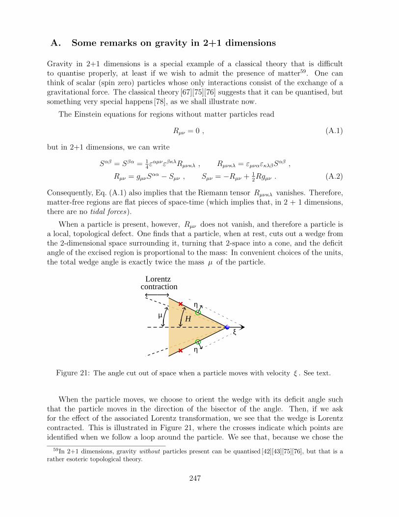
A. Some remarks on gravity in 2+1 dimensions

Gravity in 2+1 dimensions is a special example of a classical theory that is difficultto quantise properly, at least if we wish to admit the presence of matter59. One canthink of scalar (spin zero) particles whose only interactions consist of the exchange of agravitational force. The classical theory [67][75][76] suggests that it can be quantised, butsomething very special happens [78], as we shall illustrate now.

The Einstein equations for regions without matter particles read

Rµν = 0 , (A.1)

but in 2+1 dimensions, we can write

Sαβ = Sβα = 14εαµνεβκλRµνκλ , Rµνκλ = εµναεκλβS

αβ ,

Rµν = gµνSαα − Sµν , Sµν = −Rµν + 1

2Rgµν . (A.2)

Consequently, Eq. (A.1) also implies that the Riemann tensor Rµνκλ vanishes. Therefore,matter-free regions are flat pieces of space-time (which implies that, in 2 + 1 dimensions,there are no tidal forces).

When a particle is present, however, Rµν does not vanish, and therefore a particle isa local, topological defect. One finds that a particle, when at rest, cuts out a wedge fromthe 2-dimensional space surrounding it, turning that 2-space into a cone, and the deficitangle of the excised region is proportional to the mass: In convenient choices of the units,the total wedge angle is exactly twice the mass µ of the particle.

contractionLorentz

H

ξ

η

η

µ

Figure 21: The angle cut out of space when a particle moves with velocity ξ . See text.

When the particle moves, we choose to orient the wedge with its deficit angle suchthat the particle moves in the direction of the bisector of the angle. Then, if we askfor the effect of the associated Lorentz transformation, we see that the wedge is Lorentzcontracted. This is illustrated in Figure 21, where the crosses indicate which points areidentified when we follow a loop around the particle. We see that, because we chose the

59In 2+1 dimensions, gravity without particles present can be quantised [42][43][75][76], but that is arather esoteric topological theory.

247

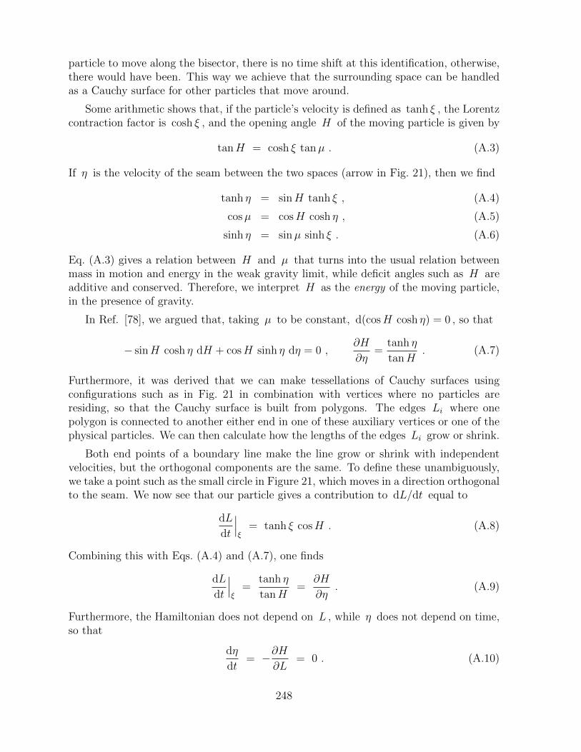
particle to move along the bisector, there is no time shift at this identification, otherwise,there would have been. This way we achieve that the surrounding space can be handledas a Cauchy surface for other particles that move around.

Some arithmetic shows that, if the particle’s velocity is defined as tanh ξ , the Lorentzcontraction factor is cosh ξ , and the opening angle H of the moving particle is given by

tanH = cosh ξ tanµ . (A.3)

If η is the velocity of the seam between the two spaces (arrow in Fig. 21), then we find

tanh η = sinH tanh ξ , (A.4)

cosµ = cosH cosh η , (A.5)

sinh η = sinµ sinh ξ . (A.6)

Eq. (A.3) gives a relation between H and µ that turns into the usual relation betweenmass in motion and energy in the weak gravity limit, while deficit angles such as H areadditive and conserved. Therefore, we interpret H as the energy of the moving particle,in the presence of gravity.

In Ref. [78], we argued that, taking µ to be constant, d(cosH cosh η) = 0 , so that

− sinH cosh η dH + cosH sinh η dη = 0 ,∂H

∂η=

tanh η

tanH. (A.7)

Furthermore, it was derived that we can make tessellations of Cauchy surfaces usingconfigurations such as in Fig. 21 in combination with vertices where no particles areresiding, so that the Cauchy surface is built from polygons. The edges Li where onepolygon is connected to another either end in one of these auxiliary vertices or one of thephysical particles. We can then calculate how the lengths of the edges Li grow or shrink.

Both end points of a boundary line make the line grow or shrink with independentvelocities, but the orthogonal components are the same. To define these unambiguously,we take a point such as the small circle in Figure 21, which moves in a direction orthogonalto the seam. We now see that our particle gives a contribution to dL/dt equal to

dL

dt

∣∣∣ξ

= tanh ξ cosH . (A.8)

Combining this with Eqs. (A.4) and (A.7), one finds

dL

dt

∣∣∣ξ

=tanh η

tanH=

∂H

∂η. (A.9)

Furthermore, the Hamiltonian does not depend on L , while η does not depend on time,so that

dη

dt= −∂H

∂L= 0 . (A.10)

248

These last two equations can be seen as the Hamilton equations for L and η . This meansthat η and L are canonically associated with one another. If there are many polygonsconnected together with seams Li , moving with transverse velocities tanh ηi , then weobtain Hamiltonian equations for their time dependence, with Poisson brackets

Li, ηj = δij . (A.11)

Thus, the lengths Li are like positions and the ηi are like the associated momenta.This clearly suggests that all one needs to do to obtain the quantum theory is to postulatethat these Poisson brackets are replaced by commutators.

A.1. Discreteness of time

There is, however, a serious complication, lying in the nature of our Hamiltonian. If wehave many particles, all adding deficit angles to the shape of our Cauchy surface, one caneasily see what might happen:

If the total energy due to matter particles exceeds the value 2π , the universewill close into itself, allowing only the value 4π for its total Hamiltonian,

assuming that the universe is simply connected. Thus, the question arises what it meansto vary the Hamiltonian with respect to η ’s, as in Eq. (A.9).

There is a way to handle this question: consider some region X in the universe Ω ,and ask how it evolves with respect to data in the rest of the universe, Ω\X . The problemis then to define where the boundary between the two regions X and Ω\X is.

An other peculiar feature of this Hamiltonian is that it is defined as an angle (evenif it might exceed the value 2π ; it cannot exceed 4π ). In the present work, we becamequite familiar with Hamiltonians that are actually simple angles: this means that theirconjugate variable, time, is discrete. The well-defined object is not the Hamiltonian itself,but the evolution operator over one unit of time: U = e−iH . Apparently, what we aredealing with here, is a world where the evolution goes in discretised steps in time.

The most remarkable thing however, is that we cannot say that the time for the entireuniverse is discrete. Global time is a meaningless concept, because gravity is a diffeo-morphism invariant theory. Time is just a coordinate, and physical states are invariantunder coordinate transformations, such as a global time translation. It is in regions wherematter is absent where we have local flatness, and only in those regions, relative timeis well-defined, and as we know now, discrete. Because of the absence of a global timeconcept, we have no Schrodinger equation, or even a discrete time-step equation, thattells us how the entire universe evolves.

Suppose we split the universe Ω into two parts, X and Ω\X . Then the edges Liin X obey a Schrodinger equation regarding their dependence on a relative time variablet (it is relative to time in Ω\X ). The Schrodinger equation is derived from Eq. (A.5),where now H and η are operators:

η = −i ∂∂L

, H = i∂

∂t. (A.12)

249

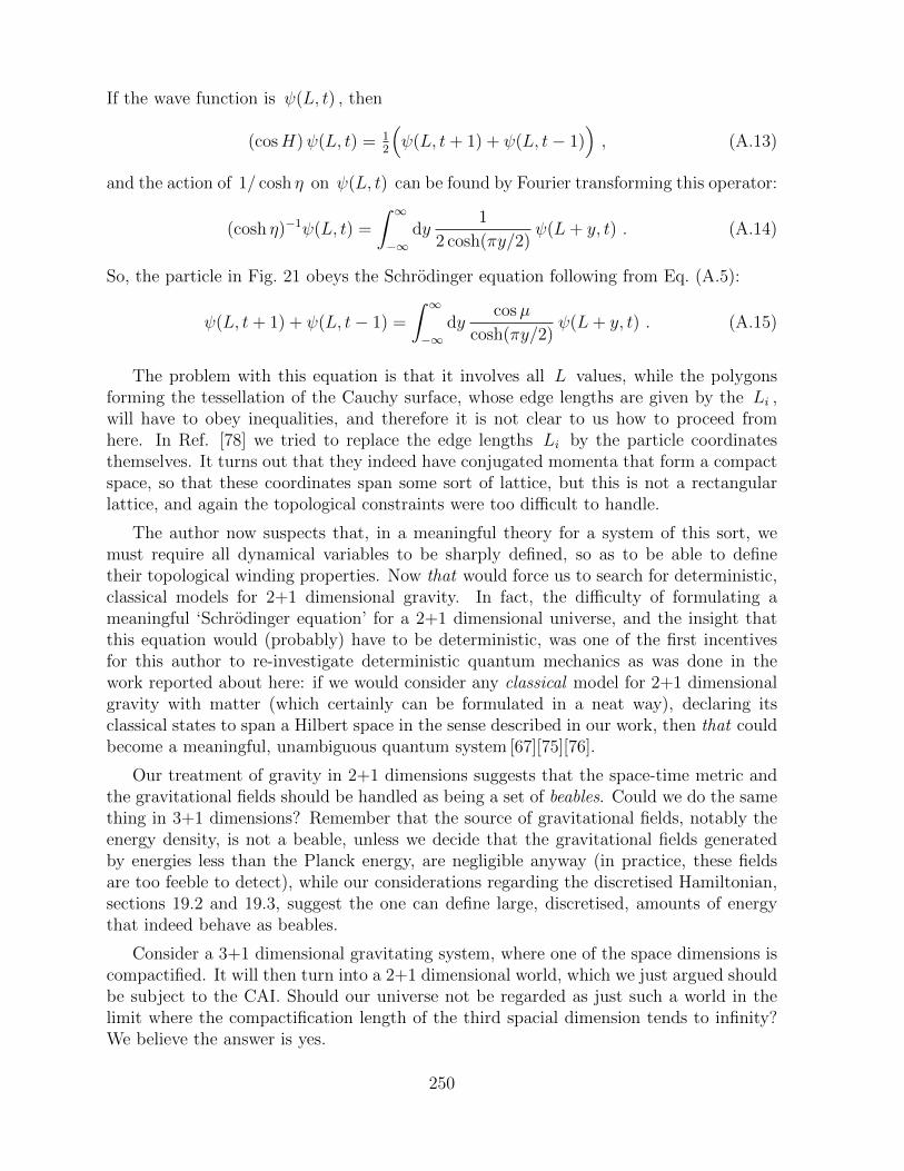
If the wave function is ψ(L, t) , then

(cosH)ψ(L, t) = 12

(ψ(L, t+ 1) + ψ(L, t− 1)

), (A.13)

and the action of 1/ cosh η on ψ(L, t) can be found by Fourier transforming this operator:

(cosh η)−1ψ(L, t) =

∫ ∞−∞

dy1

2 cosh(πy/2)ψ(L+ y, t) . (A.14)

So, the particle in Fig. 21 obeys the Schrodinger equation following from Eq. (A.5):

ψ(L, t+ 1) + ψ(L, t− 1) =

∫ ∞−∞

dycosµ

cosh(πy/2)ψ(L+ y, t) . (A.15)

The problem with this equation is that it involves all L values, while the polygonsforming the tessellation of the Cauchy surface, whose edge lengths are given by the Li ,will have to obey inequalities, and therefore it is not clear to us how to proceed fromhere. In Ref. [78] we tried to replace the edge lengths Li by the particle coordinatesthemselves. It turns out that they indeed have conjugated momenta that form a compactspace, so that these coordinates span some sort of lattice, but this is not a rectangularlattice, and again the topological constraints were too difficult to handle.

The author now suspects that, in a meaningful theory for a system of this sort, wemust require all dynamical variables to be sharply defined, so as to be able to definetheir topological winding properties. Now that would force us to search for deterministic,classical models for 2+1 dimensional gravity. In fact, the difficulty of formulating ameaningful ‘Schrodinger equation’ for a 2+1 dimensional universe, and the insight thatthis equation would (probably) have to be deterministic, was one of the first incentivesfor this author to re-investigate deterministic quantum mechanics as was done in thework reported about here: if we would consider any classical model for 2+1 dimensionalgravity with matter (which certainly can be formulated in a neat way), declaring itsclassical states to span a Hilbert space in the sense described in our work, then that couldbecome a meaningful, unambiguous quantum system [67][75][76].

Our treatment of gravity in 2+1 dimensions suggests that the space-time metric andthe gravitational fields should be handled as being a set of beables. Could we do the samething in 3+1 dimensions? Remember that the source of gravitational fields, notably theenergy density, is not a beable, unless we decide that the gravitational fields generatedby energies less than the Planck energy, are negligible anyway (in practice, these fieldsare too feeble to detect), while our considerations regarding the discretised Hamiltonian,sections 19.2 and 19.3, suggest the one can define large, discretised, amounts of energythat indeed behave as beables.

Consider a 3+1 dimensional gravitating system, where one of the space dimensions iscompactified. It will then turn into a 2+1 dimensional world, which we just argued shouldbe subject to the CAI. Should our universe not be regarded as just such a world in thelimit where the compactification length of the third spacial dimension tends to infinity?We believe the answer is yes.

250

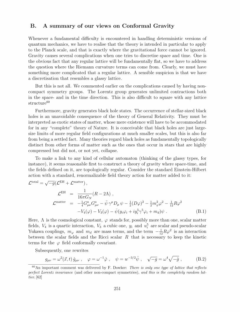
B. A summary of our views on Conformal Gravity

Whenever a fundamental difficulty is encountered in handling deterministic versions ofquantum mechanics, we have to realise that the theory is intended in particular to applyto the Planck scale, and that is exactly where the gravitational force cannot be ignored.Gravity causes several complications when one tries to discretise space and time. One isthe obvious fact that any regular lattice will be fundamentally flat, so we have to addressthe question where the Riemann curvature terms can come from. Clearly, we must havesomething more complicated that a regular lattice. A sensible suspicion is that we havea discretisation that resembles a glassy lattice.

But this is not all. We commented earlier on the complications caused by having non-compact symmetry groups. The Lorentz group generates unlimited contractions bothin the space- and in the time direction. This is also difficult to square with any latticestructure60

Furthermore, gravity generates black hole states. The occurrence of stellar-sized blackholes is an unavoidable consequence of the theory of General Relativity. They must beinterpreted as exotic states of matter, whose mere existence will have to be accommodatedfor in any “complete” theory of Nature. It is conceivable that black holes are just large-size limits of more regular field configurations at much smaller scales, but this is also farfrom being a settled fact. Many theories regard black holes as fundamentally topologicallydistinct from other forms of matter such as the ones that occur in stars that are highlycompressed but did not, or not yet, collapse.

To make a link to any kind of cellular automaton (thinking of the glassy types, forinstance), it seems reasonable first to construct a theory of gravity where space-time, andthe fields defined on it, are topologically regular. Consider the standard Einstein-Hilbertaction with a standard, renormalizable field theory action for matter added to it:

Ltotal =√−g(LEH + Lmatter) ,

LEH =1

16πGN

(R− 2Λ) ,

Lmatter = −14GaµνG

aµν − ψ γµDµ ψ − 1

2(Dϕ)2 − 1

2m2ϕϕ

2 − 112Rϕ2

−V4(ϕ)− V3(ϕ)− ψ(yiϕi + iy5i γ

5ϕi +md)ψ . (B.1)

Here, Λ is the cosmological constant, ϕ stands for, possibly more than one, scalar matterfields, V4 is a quartic interaction, V3 a cubic one, yi and u5

i are scalar and pseudo-scalarYukawa couplings, mϕ and md are mass terms, and the term − 1

12Rϕ2 is an interaction

between the scalar fields and the Ricci scalar R that is necessary to keep the kineticterms for the ϕ field conformally covariant.

Subsequently, one rewrites

gµν = ω2(~x, t) gµν , ϕ = ω−1ϕ , ψ = w−3/2ψ ,√−g = ω4

√−g , (B.2)

60An important comment was delivered by F. Dowker: There is only one type of lattice that reflectsperfect Lorentz invariance (and other non-compact symmetries), and this is the completely random lat-tice. [62]

251

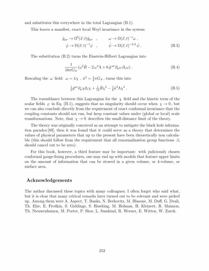
and substitutes this everywhere in the total Lagrangian (B.1).

This leaves a manifest, exact local Weyl invariance in the system:

gµν → Ω2(~x, t)gµν , ω → Ω(~x, t)−1ω ,

ϕ→ Ω(~x, t)−1ϕ , ψ → Ω(~x, t)−3/2 ψ . (B.3)

The substitution (B.2) turns the Einstein-Hilbert Lagrangian into

1

16πGN

(ω2R− 2ω4Λ + 6 g µν∂µω ∂νω) . (B.4)

Rescaling the ω field: ω = κχ , κ2 = 43πGN , turns this into

12gµν∂µχ∂νχ+ 1

12Rχ2 − 1

6κ2Λχ4 . (B.5)

The resemblance between this Lagrangian for the χ field and the kinetic term of thescalar fields ϕ in Eq. (B.1), suggests that no singularity should occur when χ→ 0 , butwe can also conclude directly from the requirement of exact conformal invariance that thecoupling constants should not run, but keep constant values under (global or local) scaletransformations. Note, that χ→ 0 describes the small-distance limit of the theory.

The theory was originally conceived as an attempt to mitigate the black hole informa-tion paradox [89], then it was found that it could serve as a theory that determines thevalues of physical parameters that up to the present have been theoretically non calcula-ble (this should follow from the requirement that all renormalization group functions βishould cancel out to be zero).

For this book, however, a third feature may be important: with judiciously chosenconformal gauge-fixing procedures, one may end up with models that feature upper limitson the amount of information that can be stowed in a given volume, or 4-volume, orsurface area.

Acknowledgements

The author discussed these topics with many colleagues; I often forget who said what,but it is clear that many critical remarks later turned out to be relevant and were pickedup. Among them were A. Aspect, T. Banks, N. Berkovitz, M. Blasone, M. Duff, G. Dvali,Th. Elze, E. Fredkin, S. Giddings, S. Hawking, M. Holman, H. Kleinert, R. Maimon,Th. Nieuwenhuizen, M. Porter, P. Shor, L. Susskind, R. Werner, E. Witten, W. Zurek.

252

References

[1] E. Noether, Invariante Variationsprobleme, Nachr. Konig. Gesellsch. Wiss. Gotting-en, Math-phys. Klasse 1918: 235257; N. Byers, E. Noether’s Discovery of the DeepConnection Between Symmetries and Conservation Laws, in Proceedings of a Sym-posium on the Heritage of Emmy Noether, held on 24 December 1996, at the Bar-IlanUniversity, Israel, Appendix B, 1998.

[2] M. Born, Zur Quantenmechanik der Stoßvorgange (German) [Toward the quan-tum mechanics of collision processes], j-z-physik, 37 (1926) 863–867; id., j-z-physik,38(1026) 803–827.

[3] L. de Broglie, presentation at the Solvay Conference, 1928, Electrons et Photons:Rapports et Discussions du Cinquieme Conseil de Physique tenu a Bruxelles du 24au 29 Octobre 1927 sous les auspices de l’Institut International Physique Solvay.

[4] P. Jordan and E. Wigner, Uber das Paulische Aquivalenzverbot, Z. Phys. 47 (1928)631.

[5] J. von Neumann, Mathematical Foundations of Quantum Mechanics (German edi-tion 1932), Princeton: Princeton University Press.

[6] A. Einstein, B. Podolsky and N. Rosen, Can Quantum mechanical description ofphysical reality be considered complete?, Phys. Rev. 47 (1935) 777; M. Jammer, Theconceptual Development of Quantum Mechanics, (Mc. Graw-Hill, 1966);

[7] Grete Hermann, Die naturphilosophischen Grundlagen der Quantenmechanik, Natur-wissenschaften, Volume 23, Number 42, 718-721 (1935), doi:10.1007/BF01491142(preview in German)

[8] E. Schrodinger, Die gegenwartige Situation in der Quantenmechanik, Die Naturwis-senschaften, 23 (1935) 807-812; 823-828; 844-849 [A 207d]. Transl.: The presentsituation in quantum mechanics, Translator: John D. Trimmer, Proc. of the Ame.Philosophical Society, 124, 323-38; section I.11 of part I of Quantum Theory andMeasurement (J.A. Wheeler and W.H. Zurek, eds.), Princeton university Press, NewJersey 1983.

[9] B. Kaufman, Crystal Statistics. II. Partition Function Evaluated by Spinor Analysis,Phys. Rev. 76 (1949) 1232.

[10] D. Bohm, A Suggested Interpretation of the Quantum Theory in Terms of “HiddenVariables, I”. Phys. Rev. 85 (1952) 166 - 179; id., II. Phys. Rev. 85 (1952) 180 - 193.

[11] E.C.G. Stueckelberg and A. Peterman, La normalization des constantes dans latheorie des quanta, Helv. Phys. Acta 26 (1953) 499.

[12] H. Everett, Relative State Formulation of Quantum Mechanics, Reviews of Mod.Phys. 29 (1957) 454.

253

[13] A.M. Gleason, Measures on the closed subspaces of a Hilbert space, Journal of Math-ematics and Mechanics 6 (1957) 885.

[14] J. Goldstone, Field theories with superconductor solutions, Nuovo Cim. 19 (1961) 154;Y. Nambu and G. Jona-Lasinio, Dynamical Model of Elementary Particles Based onan Analogy with Superconductivity. I, Phys. Rev. 122 (1961) 345.

[15] E. Merzbacher, Quantum mechanics, John Wiley & Sons, New York and London,1961.

[16] A.S. Davidov, Quantum mechanics, transl and edited by D. ter Haar, PergamonPress, Oxford, London, Edinburgh, New York, Paris, Frankfurt, 1965.

[17] R.J. Glauber, Coherent and incoherent states of radiation field, Phys. Rev. 131 (1963)2766.

[18] J. S. Bell, On the Einstein Podolsky Rosen Paradox, Physics 1 (1964) 195.

[19] Konrad Zuse, 1969, Rechnender Raum. Braunschweig: Friedrich Vieweg & Sohn,transl: Calculating Space, MIT Technical Translation AZT-70-164-GEMIT, Mas-sachusetts Institute of Technology (Project MAC), Cambridge, Mass. 02139. AdrianGerman and Hector Zenil (eds).

[20] J.F. Clauser, M.A. Horne, A. Shimony, and Rc.A. Holt, Proposed experiment to testlocal hidden-variable theories, Phys. Rev. Lett. 23 (15): 8804, doi:10.1103 / Phys RevLett. 23.880.

[21] B.S. DeWitt,Quantum Mechanics and Reality, Physics Today 23 (9) pp 30-40 (1970),id., The Many-Universes Interpretation of Quantum Mechanics, Proceedings of theInternational School of Physics ”Enrico Fermi” Course IL: Foundations of QuantumMechanics, Academic Press (1972).

[22] M. Gardner, The fantastic combinations of John Conway’s new solitary game “life”,Scientific American, 223 (4) (1970); On cellular automata, self-reproduction, theGarden of Eden and the game “life”, ibid., 224 (2) (1971).

[23] C.G. Callan, Broken Scale Invariance in Scalar Field Theory, Phys. Rev. D2 (1970)1541.

[24] K. Symanzik, Small Distance Behaviour in Field Theory and Power Counting, Com-mun. Math. Phys. 18, 227 (1970).

[25] H.D. Zeh, On the Interpretation of Measurement in Quantum Theory, Foundation ofPhysics, 1 (1970) 69.

[26] S.R. Coleman, There are no Goldstone bosons in two dimensions, Commun Math.Phys. 31 (1973) 259.

254

[27] I. S. Gradshteyn and I. M. Ryzhik’s Table of Integrals, Series, and Products, A.Jeffrey and D, Zwillinger (eds.), ISBN 0-12-294757-6; see also: A. Dieckmann,http://pi.physik.uni-bonn.de/˜dieckman/InfProd/InfProd.html.

[28] S.W. Hawking, Particle Creation by Black Holes, Commun. Math. Phys. 43 (1975)199, Erratum ibid. 46 (1976) 206; J.B. Hartle and S.W. Hawking, Path Integralderivation of black hole radiance, Phys.Rev. D13 (1976) 2188

[29] C. Itzykson and J-B. Zuber, Quantum Field Theory, Mc.Graw-Hill, Singapore, 1980,ISBN 0-07-066353-X; L.H. Ryder, Quantum Field Theory, Cambridge Univ. Press,1985. 1996, ISBN 0 521 47242.3.

[30] J. D. Bekenstein, A universal upper bound to the entropy to energy ratio for boundedsystems, Phys. Rev. D23, 287 (1981)

[31] J. S. Bell, On the impossible pilot wave, Foundations of Physics 12 (1982) 989; id.,Speakable and unspeakable in quantum mechanics (Cambridge Univ. Press, Cam-bridge, 1987).

[32] A. Aspect, J. Dalibard and G. Roger, Experimental Realization of Einstein-Podolsky-Rosen-Bohm Gedankenexperiment: A New Violation of Bell’s Inequalities,Phys. Rev. Letters, 49 (1982) 91; id., Experimental Test of Bell’s Inequalities UsingTime-Varying Analyzers, Phys. Rev. Letters, doi:10.1103 / PhysRevLett. 49.1804;

[33] P. Pearle, Reduction of the State Vector by a Nonlinear Schrodinger Equation,Phys. Rev. D 13 (1976) 857; id., Might God toss coins?, Found. Phys. 12 (1982)249.

[34] A.A. Sagle and R.E. Walde, Introduction to Lie groups and Lie algebras, Aca-demic Press, New York, 1973, ISBN 0-12-614-550-4. 49, Iss. 25, 1804 (1982) doi:10.1103/PhysRevLett.49.1804.

[35] E. Fredkin and T. Toffoli, Int.J.Theor.Phys. 21 (1982) 219; D.B. Miller and E. Fred-kin, Two-state, Reversible, Universal cellular Automata in Three Dimensions, Proc.2nd Conf. on Computing Frontiers, Ischia, Italy: ACM 45, doi: 10.1145/1062271,arXiv:nlin/0501022.

[36] B. de Wit and J. Smith, Field Theory in Particle Physics, Vol I, North-HollandElsevier, Amsterdam, Oxf., New Y., Tokyo, 1986, ISBN 0-444-86-999-9.

[37] A. Das and A. Melissinos, Quantum Mechanics, A Modern Introduction, Gordon andBreach, Ne York, London, Paris, Montreux, Tokyo, Melbourne, 1986.

[38] G.C. Ghirardi, A. Rimini and T. Weber, Unified dynamics for microscopic and macro-scopic systems, Phys. Rev. D 34 (1986) 470.

[39] M.B. Green, J.H. Schwarz and E. Witten, Superstring Theory, Cambridge Univ.Press, 1987, ISBN 0 521 32384 3.

255

[40] C.H. Brans, Bell’s Theorem Does Not Eliminate Fully Causal Hidden Variables, Int.J. Theor. Physics, 27 No 2 (1988) 219.

[41] I. Klebanov and L. Susskind, Continuum strings from discrete field theories,Nucl. Physics B 309 (1988) 175.

[42] E. Witten, 2+1 Gravity as an Exactly Soluble Model, Nucl. Phys. B311 (1988) 46-78.

[43] St. Carlip, Exact quantum scattering in 2+1 dimensional gravity, Nucl. Phys. B324(1989) 106-122; id., (2+1)-dimensional Chern-Simons gravity as a Dirac square root,Phys, Rev. D45 (1992) 3584-3590.

[44] A. Pais, Niets Bohr’s Times, in physics, philosophy, and polity, Clarendon Press,Oxford 1991, ISBN 0-19-852049-2.

[45] W.H. Zurek, Decoherence and the transition from quantum to classical, Physics To-day, 44 36 (1991).

[46] D.E. Sands, Introduction to Crystallography (Dover Classics of Science andMathematics) (Paperback - January 1994), ISBN 10: 0486678393 / ISBN 13:9780486678399.

[47] L. Susskind, The World as a Hologram, J. Math. Phys. 36 (1995) 6377, hep-th/

9409089.

[48] C. Torrence and G.P. Compo, A Practical Guide to Wavelet Analysis, Progr. inAtmospheric and Oceanic Sciences, Boulder, Colorado, Bulletin of the AmericanMeteorological Sociwty, October 1997.

[49] J.G. Polchinski, Introduction to the Bosonic String, String Theory Vol (I), CambridgeUniv. Press, 1998, ISBN 0 521 63303 6; id., Superstring Theory and Beyond, StringTheory Vol (II), Cambridge Univ. Press 1998, ISBN 0521 63304 4.

[50] A. Kempf, A Generalized Shannon Sampling Theorem, Fields at the Planck Scale asBandlimited Signals, Phys.Rev.Lett. 85 (2000) 2873.

[51] M. Blasone, P. Jizba and G. Vitiello, Dissipation and Quantization, hep-th/0007138.

[52] S. Wolfram, A New Kind of Science, Champaign, IL: Wolfram Media, Inc. (2002).ISBN 1-57955-008-8. OCLC 47831356; http://www.wolframscience.com

[53] A. Bassi and G.C. Ghirardi, Dynamical reduction models, Phys. Rep. 379 (2003) 257.

[54] M. Schlosshauer, Decoherence, the measurement problem, and interpretations ofquantum mechanics, Reviews of Mod. Phys., Vol 76, No. 4 (2004) 1267, arXiv:quant-ph/0312059.

[55] S.L. Adler, Quantum Theory as an Emergent Phenomenon, Cambridge UniversityPress, 2004.

256

[56] W.H. Zurek, Quantum origin of quantum jumps: Breaking of unitary symme-try induced by information transfer in the transition from quantum to classical,Phys. Rev. A 76, 052110 (2007), arXiv:quant-ph/0703160.

[57] M. Seevinck, Parts and Wholes. An Inquiry into Quantum and Classical Correl-ations, thesis presented at Utrecht University on October 27, 2008,arXiv:0811.1027[quant-ph].

[58] J. Conway, in New Scientist, 6 may 2006, p. 8: Free will - you only think you have it.

[59] J. Conway and S. Kochen, The Strong Free Will Theorem, arXiv:0807.3286

[quant-ph].

[60] J.Bub, Von Neumann’s ’No Hidden Variables’ Proof: A Re-Appraisal. Foundationsof Physics 40 (9-10): 13331340. (2010), doi:10.1007/s10701-010-9480-9.

[61] S. Hossenfelder, Testing super-deterministic hidden variables theories, Found. Phys.41 (2011) 1521 [arXiv:1105.4326 [quant-ph]], arXiv:1105.4326; id., Testing superde-terministic conspiracy, Journal of Physics: Conference Series 504 (2014) 012018doi:10.1088/1742-6596/504/1/012018.

[62] F. Dowker, Spacetime discreteness, Lorentz invariance and locality, J.Phys.Conf.Ser.306 (2011) 012016. DOI: 10.1088/1742-6596/306/1/012016.

[63] L. Vervoort, Bell’s Theorem: Two Neglected Solutions, Found Phys DOI 10.10701-013-9715-7, ArXiv 1203.6587v2.

[64] J.S. Gallicchio, A.S. Friedman, and D.I. Kaiser, Testing Bell’s Inequality with CosmicPhotons: Closing the Setting-Independence Loophole, Phys. Rev. Lett. 112 110405(2014), DOI:10.1103/PhysRevLett.112.110405, arXiv:1310.3288 [quant-ph].

[65] H-Th Elze, Quantumness of discrete Hamiltonian cellular automata, arXiv:1407.2160[quant-ph] 8 Jul 2014.

Papers by the author that are related to the subject of this work:

[66] G. ’t Hooft and M. Veltman, DIAGRAMMAR, CERN Report 73/9 (1973), reprintedin “Particle Interactions at Very High Energies”, Nato Adv. Study Inst. Series, Sect.B, vol. 4b, p. 177

[67] S. Deser, R. Jackiw and G. ’t Hooft, Three-dimensional Einstein gravity: dynamicsof flat space , Ann. Phys. 152 (1984) 220.

[68] G. ’t Hooft, On the quantum structure of a black hole, Nucl. Phys. B256 (1985) 727.

[69] On the quantization of space and time, Proc. of the 4th seminar on Quantum Gravity,May 25-29, 1987, Moscow, USSR. Eds. M.A. Markov, V.A. Berezin and V.P. Frolov,World Scientific 1988, p.551-567.

257

[70] Equivalence relations between deterministic and quantummechanical systems, J. Stat.Phys. 53 (1988) 323-344.

[71] Black holes and the foundations of quantum mechanics, In: Niels Bohr: Physics andthe World. Proc. of the Niels Bohr Centennial Symposium, Boston, MA, USA, Nov.12-14, 1985. Eds. H. Feshbach, T. Matsui and A Oleson. Publ. by Harwood AcademicPubl. GmbH (1988) p. 171-182.

[72] Quantization of discrete deterministic theories by Hilbert space extension, Nucl.Phys. B342 (1990) 471.

[73] G. ’t Hooft, K. Isler and S. Kalitzin, Quantum field theoretic behavior of a determin-istic cellular automaton, Nucl. Phys. B 386 (1992) 495;

[74] G. ’t Hooft, Dimensional Reduction in Quantum Gravity, Essay dedicated to AbdusSalam, Utrecht preprint THU-93/26; gr-qc/9310026;

[75] Classical N-particle cosmology in 2+1 dimensions, Class. Quantum Grav. 10 (1993)S79-S91.

[76] Cosmology in 2+1 dimensions, Nucl. Phys. B30 (Proc. Suppl.) (1993) 200-203.

[77] The scattering matrix approach for the quantum black hole: an overview. J. Mod.Phys. A11 (1996) pp. 4623-4688. gr-qc/9607022.

[78] Quantization of point particles in (2+1)-dimensional gravity and space-time discrete-ness, Class. Quantum Grav. 13 1023-1039.

[79] Quantum Gravity as a Dissipative Deterministic System, Class. Quant. Grav. 16(1999) 3263, arXiv:gr-qc/9903084.

[80] Determinism in Free Bosons, Int. J. Theor. Phys. 42 (2003) 355, arXiv:hep-th/0104080.

[81] The Holographic Mapping of the Standard Model onto the Black Hole Horizon, PartI: Abelian Vector Field, Scalar Field and BEH Mechanism, Class. Quantum Grav.22 (2005) 4179-4188, ITP-UU-05/17, SPIN-05/13, gr-qc/0504120 (Note: some signcorrections and further elucidations in the published version).

[82] The Black Hole Horizon as a Dynamical System, Int. Conf. on Einstein’s Legacy inthe New Millennium, Dec. 15-22, 2005, Puri, India, Int. J. Mod. Physics D15 No.10(2006) 1587 - 1602; arXiv:gr-qc/0606026.

[83] The Conceptual Basis of Quantum Field Theory, in Handbook of the Philosophy ofScience, Philosophy of Physics, edited by: Jeremy Butterfield et al, Elsevier, ISBN:978-0-444-51560-5, Part A, pp. 661-729 (2007).

[84] The Free-Will Postulate in Quantum Mechanics, ITP-UU-07/4, SPIN-07/4, arXiv:quant-ph/0701097.

258

[85] Emergent quantum mechanics and emergent symmetries, presented at PASCOS13, Imperial College, London, July 6, 2007; ITP-UU-07/39, SPIN-07/27; arXiv:

hep-th/0707.4568.

[86] Entangled quantum states in a local deterministic theory, 2nd Vienna Symposiumon the Foundations of Modern Physics (June 2009), ITP-UU-09/77, SPIN-09/30;arXiv:0908.3408v1 [quant-ph].

[87] Hilbert space in deterministic theories, a reconsideration of the interpretation of quan-tum mechanics, in Proceedings of the 3rd Stueckelberg Workshop on Relativistic FieldTheories, N. Carlevaro, R. Ruffini and G.V. Vereshchagin, eds., Cambridge ScientificPubl., 2010. pp. 1-18;

[88] Classical cellular Automata and Quantum Field Theory, in Proceedings of the Con-ference in Honour of Murray Gell-Mann’s 80th Birthday, on Quantum Mechan-ics, Elementary Particles, Quantum Cosmology and Complexity, Singapore, Febru-ary 2010, H.Fritzsch and K.K.Phua, eds., World Scientific, pp 397 - 408, repr. in:Int. J. Mod. Phys. A25, no 23 (2010) 4385-4396.

[89] The Conformal Constraint in Canonical Quantum Gravity, ITP-UU-10/40, Spin-10/33, arXiv:1011.0061[gr-qc]; A class of elementary particle models without anyadjustable real parameters, Found. Physics 41, no 12, pp 1829-1856, ITP-UU-11/14,Spin-11/08, arXiv:1104.4543.

[90] “How a wave function can collapse without violating Schrodinger’s equation, andhow to understand Born’s rule”, ITP-UU-11/43, SPIN-11/34, arXiv: 1112.1811

[quant-ph].

[91] Relating the quantum mechanics of discrete systems to standard canonical quantummechanics, ITP-UU-12/14; SPIN-12/12, arXiv:1204.4926.

[92] Duality between a deterministic cellular automaton and a bosonic quantum field the-ory in 1+1 dimensions, ITP-UU-12/18; SPIN-12/16, arXiv:1205.4107.

[93] Discreteness and Determinism in Superstrings, ITP-UU-12/25; SPIN-12/23, arXiv:1207.3612[hep-th].

[94] Hamiltonian formalism for integer-valued variables and integer time steps and apossible application in quantum physics, Report-no: ITP-UU-13/29, SPIN-13/21,http://arxiv.org/abs/1312.1229.

259