During the summer of 2008, Dustin Phan held an internship with the Wiseman Research Group in Los Angeles. During that time, he learned about the clinical trial process for developing FDA approved vaccines and developed an interest in cancer. When he came back to school that Fall, Dustin was fortunate enough to find Dr. John S. Lowengrub working on mathematical can-cer modeling. He worked with Dr. Lowengrub in develop-ing and analyzing a discrete mathematical model of solid tumor growth called a cellu-lar automaton model. Dustin was accepted into the UCI Mathematical, Computation, and Systems Biology graduate program, allowing him to con-tinue research in both fields after graduation. Cancer cells compete with each other and host cells in a fast paced

evolutionary system. Typically, mutations are introduced into the genome of cancer cells, and it is important to understand what types of mutations ensure that one mutant is more fit than another and is also more fit than the host cells. This work uses a mathemati-cal model that tracks the motion and interaction of discrete cells. The results demonstrate that there is a nontrivial trade-off between migration and proliferation. This can have profound implications

for traditional cancer treatment, which typically only targets highly proliferative cells. Being involved in state-of-the-art research, such as described in this paper, provides undergraduates with a unique opportunity to bridge classroom mathematics experi-ence and knowledge with real world applications.

Key Te rmsCell Motility

Cellular Automaton

Discrete Modeling

Invasion Time

Mathematical Modeling

Solid Tumor Growth

A Discrete Cellular Automaton Model Demonstrates Cell Moti l i ty Increases Fitness in Solid Tumors

Dustin D. PhanMathematics

John S. LowengrubSchool of Physical Sciences

Tumor growth is a complex biological process often studied through the use of both in vivo and in vitro experimentation. Mathematical models provide a com-

plementary approach by using a controlled environment in which a system can be described quantitatively. This can also yield prognostic data after thorough analysis by the modeler. In an effort to study the characteristics that increase cell fitness, this paper presents a discrete cellular automaton model that uses computer simulation to describe the invasion of healthy tissue by cancer cells. A mechanistic approach is used in which the proliferation, migration, and death of cells is controlled through preset parameters. Values can be adjusted and corresponding simulations can be analyzed. During simulation, cells with high migration probabilities create morphologies with considerably less population density than those with low migration probabilities, thereby creating space into which other cells may proliferate or migrate. Furthermore, these highly migratory cells display greater rates of population growth compared to less migratory cells with the same proliferation rate. The model also shows that tumor cell invasion times can decrease even when increasing only the cells’ tendency to migrate. Results show that the population growth rate of non-migratory cells may be achieved by cells with smaller proliferation rates but larger migration rates.

5 5 T H E U C I U N D E R G R A D U A T E R E S E A R C H J O U R N A L

A u t h o r

A b s t r a c t

F a c u l t y M e n t o r

56 T h e U C I U n d e r g r a d u a t e R e s e a r c h J o u r n a l

A D I S C R E T E C E L L U L A R A U T O M A T O N M O D E L

Introduct ion

Tumor growth and development is a complex biological process typically beginning with genetic mutations within a single cell. Genetic irregularities typically affect two basic types of genes: oncogenes and tumor suppressor genes. In healthy cells, oncogenes are responsible for producing hormones promoting mitosis, the regulated proliferation of cells. As a result, when oncogenes mutate or become over expressed, cells begin to proliferate regardless of the pres-ence of hormones, resulting in uncontrolled growth (Croce, 2008). Tumor suppressor genes, however, are responsible for the regulation of the cell cycle and apoptosis. When cells become damaged or mutated, these genes arrest the pro-gression of the cell cycle in order to carry out DNA repair or to induce apoptosis, that is, programmed cellular death (Sheer, 2004). This is designed to prevent any further muta-tions from being passed on to daughter cells. Therefore, any mutations in tumor suppressor genes causing loss of function may allow cells to avoid apoptosis and enable the propagation of mutations and damaged DNA to daughter cells (Barnes et al., 1993).

This paper seeks to investigate the characteristics making certain cells more fit than others in a highly competitive environment where success is determined by the cell’s abil-ity to propagate genetic material. The model presented in this paper focuses on two types of phenotypic changes. The first is associated with proliferation, in which the activation of oncogenes and inactivation of tumor suppressor genes lead to uncontrolled growth. The second type of mutation, however, affects cell motility. For instance, genes associated with cell motility in solid tumors have also been associated with metastasis, a crucial step in tumor development (Fidler, 1989). While proliferative cells continue to divide only so long as spatial and nutrient restrictions allow, motile cells can break away from the primary tumor and access new nutrient sources, leading to the development of secondary tumors at new sites in the body (Sahai, 2007). Therefore, studying the cellular characteristics leading to increased fit-ness is an important step toward understanding solid tumor development.

In studying tumor development, both in vitro and in vivo experimentation have been used extensively. In vivo studies typically allow researchers to perform studies on a living organism. The large number of biological variables in in vivo studies, however, makes it difficult for researchers to precisely identify all the processes involved. In vitro experi-mentation, alternatively, allows experimenters to create controlled studies of specific systems with fewer outside

variables. However, in vitro studies often do not reflect the reality of tumor development, and typically must be fol-lowed by in vivo testing in order to observe the overall effects of an experiment on a living organism.

Another means of studying biological mechanisms is through the use of mathematical and computational mod-els. Mathematical models often yield important diagnostic as well as prognostic data (Quaranta et al., 2008; Drasdo and Hohme, 2007), while computational models provide a precisely controlled environment in which the evolution of a system may be analyzed quantitatively. Simulations allow researchers to test conditions that are difficult to obtain through in vitro or in vivo experimentation, and can often rule out particular mechanisms as an explanation for experimen-tal observations (Fall et al., 2002).

In the past, population models such as the Gompertzian, the Bertalanffy, the exponential, and the logistic models have all been proposed as possible representations for the growth of solid tumors (Vinayg and Frank, 1982). However, each of these mathematical models describes only the overall increase in the number of tumor cells through population dynamics, and does not distinguish among detailed cellular processes, thus limiting the predictive capability. Another approach to the mathematical modeling of tumors is the use of deterministic partial differential equations to model processes such as the growth, differentiation, diffusion, and mutations of tumor cells (Wodarz and Komarova, 2005). Examples include reaction-diffusion equations, which are used to model the spatial spread of tumors and the chemi-cal reactions involved (Ward and King, 1999; Gatenby and Gawlinski, 1996), or the continuum mechanics models, which treat tumors as a collection of tissue while also con-sidering physical forces and pressure between cells (Tracqui, 1995; Greenspan, 1976). These types of models often describe the tumor as a whole, and are unable to capture the stochastic nature of tumors at the cellular and sub-cellular levels (Anderson et al., 2005).

This study uses a different type of model for tumor growth: the discrete cellular automaton model. In cellular automaton models, a spatial grid is first used to represent a host tissue, whereupon “cells” can be placed within the grid to repre-sent invading tumor cells. Then, through the use of sto-chastic interaction rules based on biological processes (e.g. cell cycle, mitosis), tumor growth patterns can be simulated. Thus, cellular automaton models are capable of describ-ing tumors at the cellular level, while still capturing the stochastic nature of cell behavior (Deutsch and Dormann, 2005; Anderson et al., 2005). The model presented here is

57T H E U C I U N D E R G R A D U A T E R E S E A R C H J O U R N A L

D u s t i n D . P h a n

different from much of the recent literature in which many biological processes and intricacies are modeled using cel-lular automata. Smolle and Stettner, for example, present a cellular automaton model in which autocrine and paracrine growth factors influence cell division, migration, and death, resulting in varying morphological patterns (1993). Gerlee and Anderson, in contrast, present a model investigating the impact of the micro-environment on the appearance of motile phenotypes, showing that tumors growing in harsh micro-environments are more likely to contain aggressive invasive phenotypes (2009), while Kansal et al. develops a complex three-dimensional cellular automaton describing brain tumors (2000). This paper, on the other hand, pres-ents a mathematical model of tumor growth focusing on only two forces, proliferation and migration, and how they trade off to influence the overall fitness of cells. While the model presented here is simpler, it is unique in that the deci-sion to proliferate requires multiple signals during which the cell may still migrate, creating a more realistic representation of cell dynamics. This provides insight that can then be car-ried over to more complex models.

Mathematical Model

Tissue ModelThe host tissue is represented by a two-dimensional matrix containing n x n lattice sites. Each lattice site carries a value of 0 or 1, where 0 represents open space into which tumor cells can invade and 1 denotes a site occupied by a tumor cell. Time is measured in the number of evolution steps.

Possible Cell ActionsAt the start of each time step, a tumor cell either dies or survives. Cells that survive carry out one of three possible actions: proliferation, migration, or quiescence. Parameters governing cell mechanisms at each time step are defined in Table 1.

Cell Survival and Death. For simplicity, each tumor cell has an equal probability of surviving or dying, with the probabili-ties of survival and death given by Ps and Pd, respectively, where:

Ps + Pd = 1 (1)

To determine the course of action for each tumor cell, a uniformly distributed random number 0 ≤ rr ≤ 1 is gener-ated and compared against the parameter Ps. If rr < Ps, the cell will survive and will continue to migrate, proliferate, or quiesce during its next time step. However, if rr ≥ Ps, the respective tumor cell will die. In this case, the lattice site previously occupied and set to 1 will empty and change to 0, creating an empty site, which allows other tumor cells to occupy it through migration or proliferation.

Cell Proliferation. Initially, PH=0. Cell proliferation is simulat-ed by first generating a uniformly distributed random num-ber 0 ≤ rrp ≤ 1. For rrp ≥ Pp no proliferation is performed, and the model continues to test for the possibility of migra-tion as shown in the following section. When rrp < Pp one proliferation signal is obtained; that is,

PH := PH + 1 (2)

The process is repeated until the total number of prolifera-tions signals PH = NP, then the tumor cell will proceed to proliferate. However, if PH < NP then the cell may migrate without proliferating, as seen in the flowchart (Figure 2). Proliferation is simulated using the system shown in Equation 3 to determine the direction of proliferation (Figure 1). First, a uniformly distributed random num-ber rr is selected. If 0 ≤ rr ≤ P1 , then the site chosen for proliferation is ηi-1, j. For P1 < rr ≤ P1 + P2, ηi+1, j is chosen. If P1 + P2 < rr ≤ P1 + P2 + P3, ηi, j-1 is chosen. Finally, for P1 + P2 + P3 < rr ≤ 1, ηi, j+1 is chosen for proliferation. Once an empty site is chosen, the value of the original cell ηi, j = 1, and the position occupied by the daughter cell changes from 0 to 1. Thus the proliferating cell ηi, j maintains its original position while its daughter cell occupies the chosen lattice adjacent site. Then PH = 0 for both the daughter cell and the original cell.

Table 1Definition of Model Parameters.

Ps Probability of cell survival.

Pd Probability of cell death.

Pm Probability of cell migration.

Pp Probability of cell proliferation.

Pq Probability of cell quiescence.

rr Random value to determine survival.

rrm Random value to determine migration.

rrp Random value to determine proliferation.

PH Number of proliferation signals.

NP Total PH needed to proliferate.

Figure 1The current position of the cell is denoted by ηi, j. Possible directions of migration are given by the four adjacent quadrants.

ηi-1, j ηi, j ηi+1, j

ηi, j-1

ηi, j +1

58 T h e U C I U n d e r g r a d u a t e R e s e a r c h J o u r n a l

A D I S C R E T E C E L L U L A R A U T O M A T O N M O D E L

The probability of proliferating or migrating into each of the adjacent lattice sites is given by:

P(ηi-1, j ) = = P1

1-ηi-1, j

4 – (ηi+1, j + ηi-1, j + ηi, j +1 + ηi, j-1 )

P(ηi+1, j ) = = P2

1-ηi+1, j

4 – (ηi+1, j + ηi-1, j + ηi, j +1 + ηi, j-1 )

P(ηi, j-1 ) = = P3

1-ηi, j-1

4 – (ηi+1, j + ηi-1, j + ηi, j +1 + ηi, j-1 )

P(ηi, j+1 ) = = P4

1-ηi, j+1

4 – (ηi+1, j + ηi-1, j + ηi, j +1 + ηi, j-1 )

(3)

Cell Migration. After the survival of a tumor cell has been determined, cell migration is simulated by choosing a uni-formly distributed random number 0 ≤ rrm ≤ 1 and compar-

ing it with Pm. For values rrm ≥ Pm, the cell will quiesce and no other action will be undertaken until the next time step. For rrm < Pm, the cell may migrate. To determine the direction of migration, suppose the current position of the tumor cell is given by ηi, j; the current value of this lattice site is 1. The cell can then migrate into each of four coordi-nate directions, through the process described in the previous section, as long as the respective lattice sites are empty.

The probability of migrating into a specified lattice site is weight-ed by the number of empty sites. Consequently, when all adjacent lat-tice sites are empty, the probabil-ity of migrating into each is 0.25, whereas when all adjacent lattice sites are occupied, there is no migra-tion and the cell will quiesce. Once migration direction probabilities have been calculated and an empty lattice site has been chosen, the cell vacates its original position and occupies its neighboring site. That is, ηi, j changes from 1 to 0 and the state of the new position changes from 0 to 1. For cases where each neighbor-ing site is occupied by a tumor cell and its lattice is denoted by 1, the cell

will quiesce and no other actions will be performed. Note that cell migration is periodic. That is, if cells migrate from the edge and the leave simulated space they will return on the other side.

Cell Quiescence. Cell quiescence occurs when a tumor cell neither proliferates nor migrates. Thus, when Pp + Pm < 1 then the probability of quiescence is given by (4).

Pq = 1 – Pm – Pp (4)

Since Pp and Pm are independent, it is possible that their sum exceeds 1. For Pp + Pm ≥ 1, quiescence can only occur in a living tumor cell when the lack of space prevents pro-liferation or migration from occurring.

Update Cell Positions

No

YesYes

Yes

Yes

Yes

No

No

Initialconditions Cell Dies

No

Norrm < Pm?PH ≥ NP?

NoBeginTime Step rr < Ps?

CellSurvivesrrp < Pp ?+1 PH

Quiescent

Calculate ProliferationProbabilities

Calculate MigrationProbabilities

Migration?Proliferation?

Yes

Figure 2Simulation flowchart of mathematical model. Parameters defined as in Table 1.

59T H E U C I U N D E R G R A D U A T E R E S E A R C H J O U R N A L

D u s t i n D . P h a n

Results

General Simulation ProceduresSimulation was conducted in a domain containing 32 x 32 lattice sites. Results were collected for both NP=1 and NP=2. Because the simu-lation models a stochastic process, 100 simulations were performed for each set of parameters. Simulation and computations were performed in MATLAB.

Tumor Growth PatternsFigure 3 shows several sample simu-lation results demonstrating the spa-tiotemporal distributions of cells starting from a single cell. In each case, the probability of prolifera-tion Pp=0.25. In the simulations, NP and Pm are varied. Note that for a fixed NP, a lower probability of migration allows patterns with more densely packed cells, while large migration probabilities are associated with less densely packed cell clusters. Specifically, Figures 3a and 3b have NP=1, whereas Figures 3c and 3d have NP=2. Large migration proba-bilities are associated with a large rate of growth of the cell population. This can be attributed to the fact that higher cell motility allows tumor cells to migrate into open spaces and increase opportunities for proliferation. Comparing Figures 3a and 3b with Figures 3c and 3d also shows that NP sig-nificantly affects the evolution of the cell population. That is, simulations with NP=2 are associated with a lower rate of proliferation, leading to slower growth of cell population compared with the NP=1 simulations.

Population GrowthIn Figure 4, the cell population is plotted as a function of time by counting the number of cells at each time evolu-tion. The mean cell population generated by the model is given by the green curve; blue error bars denote the stan-dard deviation for the 100 simulations performed for each parameter set. For a fixed value of NP, simulations with Pm=0.8 (Figs 4b and 4d), demonstrate significantly faster growth before stabilizing compared to those with Pm=0.2 (Figures 4a and 4c). For Ps=1, the final population always

totals 1024 because the maximum capacity of the grid is 32 x 32. Thus, more migratory cells have faster growth rates, even when proliferation rates remain unchanged. Increasing NP, (Figures 4c and 4d) retards growth due to the increased number of proliferation hits required for a cell to prolif-erate. In addition, the standard deviation increases as NP increases, indicating more variable results. Increasing migra-tion rates also increases variability (Figure 4).

Growth rates are determined using a least squares logistic fit to Equation 5 using a method as described by Cavallini (Cavallini, 1993). The logistic growth fit of each simulation is given by the red curve (Figure 4).

dPdt

PK= rP 1 – )( (5)

Figure 3Tumor growth patterns from computer simulation at time iterations 5, 15, 25, and 35. For all four cases, Ps = 1 and Pp = 0.25. Specific parameters for each of the cases are as follows: (a). NP = 1, Pm = 0.2. (b). NP = 1, Pm = 0.8. (c). NP = 2, Pm = 0.2. (d). NP = 2, Pm = 0.8.

A

D

C

B

0

30

25

20

15

10

5

0 30252015105

0

30

25

20

15

10

5

0 30252015105

0

30

25

20

15

10

5

0 30252015105

0

30

25

20

15

10

5

0 30252015105

0

30

25

20

15

10

5

0 30252015105

0

30

25

20

15

10

5

0 30252015105

0

30

25

20

15

10

5

0 30252015105

0

30

25

20

15

10

5

0 30252015105

0

30

25

20

15

10

5

0 30252015105

0

30

25

20

15

10

5

0 30252015105

0

30

25

20

15

10

5

0 30252015105

0

30

25

20

15

10

5

0 30252015105

0

30

25

20

15

10

5

0 30252015105

0

30

25

20

15

10

5

0 30252015105

0

30

25

20

15

10

5

0 30252015105

0

30

25

20

15

10

5

0 30252015105

5 352515

60 T h e U C I U n d e r g r a d u a t e R e s e a r c h J o u r n a l

A D I S C R E T E C E L L U L A R A U T O M A T O N M O D E L

Specifically, r is the growth rate and K = 1024 is the carrying capacity. In (Figure 4a) r = 0.135, in (Figure 4b) r = 0.2167, in (Figure 4c) r = 0.0631, and in (Figure 4d) r = 0.0972. Note that increasing NP from 1 to 2 roughly halves the growth rate. Also, the logistic fit is slightly better for larger Pm because in the logistic model, all cells should prolifer-ate. This is better approximated by large Pm since there is generally more space available to cells than with smaller Pm (Figures 8 and 9).

Invasion TimeThe number of time steps until each lattice site in the host tissue is occupied by a tumor cell is defined as the invasion time. In Figure 5, the invasion time is plotted as a function of Pm for different Pp. By increasing the probability of proliferation Pp of tumor cells, the time required to invade the host tissue falls dramatically because the cells proliferate more frequently. Also note that by fixing Pp and increasing the probability of migration Pm, the invasion time decreases significantly as well, although the effect is more dramatic for small Pp. Behavior for both the NP = 1 and NP = 2 models is quantitatively similar, but note the increased invasion time for the NP = 2 model (Figure 5b). However, when NP = 2 the

invasion times tend to saturate for large enough Pm. Least squared fits were calculated for each of the curves in Figure 5. A bisection method was used to calculate Pm values for each Pp curve corresponding to the same invasion time. This allows the probability of proliferation Pp to be plotted as a function of probability of migration Pm such that the combination yields the same invasion time (Figure 6).

When NP = 1 (Figure 6a) the graphs are monotone decreas-ing, indicating that the probability of proliferation to invade at a particular time decreases as the probability of migration increases. Thus, tumor cells with low proliferation rates and high migration rates yield the same invasion times as those with higher proliferation rates but lower migration rates. When NP = 2, there appears to be a critical invasion time T* above which the dependence of Pp upon Pm for equal invasion time is non-monotone (Figure 6b). In par-ticular, for invasion times Tinv < T*inv , Pp is a monotonically decreasing function of Pm. However, for Tinv ≥ T*inv there appears to be a critical Pm* that minimizes Pp for a given invasion time. When Pm < Pm*, probability of proliferation Pp for a given invasion time is a decreasing function of Pm.

0 50 100 150 2000

100

200

300

400

500

600

700

800

900

1000

0 50 100 150 2000

100

200

300

400

500

600

700

800

900

1000

0 50 100 150 2000

100

200

300

400

500

600

700

800

900

1000

0 50 100 150 2000

100

200

300

400

500

600

700

800

900

1000

A

C

B

D

Figure 4Population as a function of time. Population: [0,1024]. Time: [0,225]. For all four cases, Pp = 0.25 and Ps = 1. Green Curve: generated by model. Red Curve: Logistic Growth Fit. Blue Lines: Standard deviation of data. Parameters are as follows: (a). NP = 1, Pm = 0.2, growth rate = 0.1350 (b). NP = 1, Pm = 0.8, growth rate = 0.2167. (c). NP = 2, Pm = 0.2, growth rate = 0.0631. (d). NP = 2, Pm = 0.8, growth rate = 0.0972.

61T H E U C I U N D E R G R A D U A T E R E S E A R C H J O U R N A L

D u s t i n D . P h a n

However, for Pm ≥ Pm*, a large Pp is required for the same invasion time.

Non-Monotonic Behavior. When NP=2 and Pp is small (i.e. Pp < 0.1), the invasion time may exhibit a non-monotone dependence on Pm (Figure 7). This gives rise to the non-

monotonicity observed in Figure 6. To study this behavior, let NC* be the cells with the necessary space to migrate or proliferate, and let NC be the total number of cells on the lattice. Then NCratio is defined to be:

NCratio = NC*

NC(6)

Thus, if NCratio = 1, all cells have the capacity to migrate or proliferate. By plotting NCratio as a function of time, one sees that NCratio decreases more slowly when the prob-ability of migration Pm is larger (Figure 8). However, when Pm is large, there is more variability as described previously. That is, the number of cells with space NC* and the total number of cells NC are equal for more time steps. This is largely due to the loosely packed morphologies in the early time steps attributed to higher migration rates. Note that for Figures 8 and 9, although NCratio and NC* should fall to 0 for each of the individual cases, the variation in values may cause the mean to shift away from 0.

0 0.1 0.2 0.3 0.4 0.5 0.6 0.7 0.8 0.9 120

40

60

80

100

120

140

160

180

200

220

Pp=0.1Pp=0.2Pp=0.3Pp=0.4Pp=0.5Pp=0.6Pp=0.7Pp=0.8Pp=0.9

A

0 0.1 0.2 0.3 0.4 0.5 0.6 0.7 0.8 0.9 10

100

200

300

400

500

600

Pp=0.1Pp=0.2Pp=0.3Pp=0.4Pp=0.5Pp=0.6Pp=0.7Pp=0.8Pp=0.9

B

Figure 5Invasion Time as a function of Pm for fixed Pp. y-Axis: Invasion Time. x-Axis: Pm. Pm: [0, 0.975]. Step size 0.025. Parameters: (a). NP = 1, Ps = 1. (b). NP=2, Ps = 1.

0 0.1 0.2 0.3 0.4 0.5 0.6 0.7 0.8 0.9 10

0.02

0.04

0.06

0.08

0.1

0.12

0.14

0.16

0.18

0.2Time=330Time=430Time=530Time=630Time=730Time=830Time=930Time=1030Time=1130Time=1230

B

0 0.1 0.2 0.3 0.4 0.5 0.6 0.7 0.8 0.9 10.0

0.05

0.1

0.15

0.2

0.25

0.3

0.35Time=60Time=100Time=140Time=180Time=220Time=260Time=300Time=340

A

Figure 6Pp as a function of Pm for fixed invasion times. y-Axis: Pp. x-Axis: Pm. Pp: [0.025, 1]. Pm: [0, 0.975]. Step size 0.025. (a). NP = 1, Ps = 1. (b). NP = 2, Ps = 1.

Figure 7Invasion Time as a function of Pm for fixed Pp. y-Axis: Invasion Time. x-Axis: Pm. Pm: [0, 0.975]. Step size 0.025. Parameters: NP = 2, Ps = 1.

0.0 0.2 0.4 0.6 0.8 1.0200

400

600

800

1000

Pp=0.05Pp=0.1

62 T h e U C I U n d e r g r a d u a t e R e s e a r c h J o u r n a l

A D I S C R E T E C E L L U L A R A U T O M A T O N M O D E L

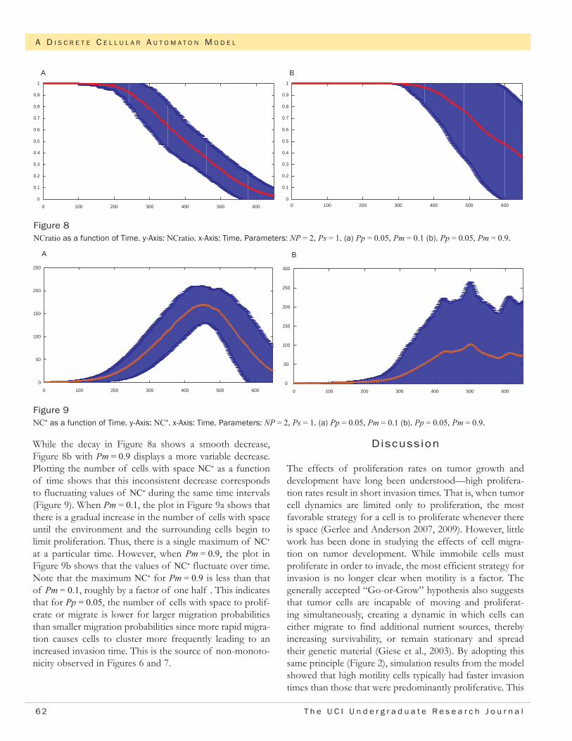
While the decay in Figure 8a shows a smooth decrease, Figure 8b with Pm = 0.9 displays a more variable decrease. Plotting the number of cells with space NC* as a function of time shows that this inconsistent decrease corresponds to fluctuating values of NC* during the same time intervals (Figure 9). When Pm = 0.1, the plot in Figure 9a shows that there is a gradual increase in the number of cells with space until the environment and the surrounding cells begin to limit proliferation. Thus, there is a single maximum of NC* at a particular time. However, when Pm = 0.9, the plot in Figure 9b shows that the values of NC* fluctuate over time. Note that the maximum NC* for Pm = 0.9 is less than that of Pm = 0.1, roughly by a factor of one half . This indicates that for Pp = 0.05, the number of cells with space to prolif-erate or migrate is lower for larger migration probabilities than smaller migration probabilities since more rapid migra-tion causes cells to cluster more frequently leading to an increased invasion time. This is the source of non-monoto-nicity observed in Figures 6 and 7.

Discussion

The effects of proliferation rates on tumor growth and development have long been understood—high prolifera-tion rates result in short invasion times. That is, when tumor cell dynamics are limited only to proliferation, the most favorable strategy for a cell is to proliferate whenever there is space (Gerlee and Anderson 2007, 2009). However, little work has been done in studying the effects of cell migra-tion on tumor development. While immobile cells must proliferate in order to invade, the most efficient strategy for invasion is no longer clear when motility is a factor. The generally accepted “Go-or-Grow” hypothesis also suggests that tumor cells are incapable of moving and proliferat-ing simultaneously, creating a dynamic in which cells can either migrate to find additional nutrient sources, thereby increasing survivability, or remain stationary and spread their genetic material (Giese et al., 2003). By adopting this same principle (Figure 2), simulation results from the model showed that high motility cells typically had faster invasion times than those that were predominantly proliferative. This

0 100 200 300 400 500 600

0

0.1

0.2

0.3

0.4

0.5

0.6

0.7

0.8

0.9

1

A

0 100 200 300 400 500 6000

0.1

0.2

0.3

0.4

0.5

0.6

0.7

0.8

0.9

1

B

Figure 8NCratio as a function of Time. y-Axis: NCratio. x-Axis: Time. Parameters: NP = 2, Ps = 1. (a) Pp = 0.05, Pm = 0.1 (b). Pp = 0.05, Pm = 0.9.

0 100 200 300 400 500 600

0

50

100

150

200

250

A

0 100 200 300 400 500 600

0

50

100

150

200

250

300

B

Figure 9NC* as a function of Time. y-Axis: NC*. x-Axis: Time. Parameters: NP = 2, Ps = 1. (a) Pp = 0.05, Pm = 0.1 (b). Pp = 0.05, Pm = 0.9.

63T H E U C I U N D E R G R A D U A T E R E S E A R C H J O U R N A L

D u s t i n D . P h a n

suggests that migratory cells were more capable of acquir-ing the space necessary to proliferate freely. Also, by keep-ing migration rates high, cells on the outer rim were able to create the necessary space for cells on the inner regions to continue proliferating, thus reducing quiescence and allow-ing more cells to remain active. These high motility cells tend to create morphologies with a large invasive area and low cell density (Figure 3), suggesting that large tumors do not necessarily contain a high number of cells (Qi et al., 1993, Gerlee and Anderson, 2009). It is also notable, however, that high migration rates coupled with very low prolifera-tion rates can result in increased invasion times, a possible result of the “Go-or-Grow” dynamic. Mathematically, we were also able to show that increasing motility may increase invasion time due to the frequent formation of cell clusters that limit the space required for proliferation and migration (Section 3.4.1). This shows that there exists an optimal com-bination of migration and proliferation for which tumor growth rate is maximized (Mansury et al., 2006).

In addition to the study of tumor morphologies and cellular behavior, the model presented in this paper was also used to study population growth. Specifically, a logistic growth fit was performed after plotting population as a function of time. This allows the investigator to estimate both the growth rate of the population and the carrying capacity of the system. Cellular automaton models have also been used in the past to model population growth, particularly the Gompertz model (Qi et al., 1993) and the logistic growth model (Hu and Ruan, 2001). In the case of Hu and Ruan, however, the cellular automaton model was based on a discretized form of the continuous logistic model. Both models are supported by extensive literature; however, these approaches do not distinguish among the details of the biological process. That is, growth models are incapable of demonstrating the dynamics of tumor growth at the cellular level. It should be noted that the cellular automaton model presented here has a better fit to the logistic model when the migration probability is large (Figure 4). In low migra-tion simulations, only cells on the outer rim are capable of proliferation or migration, while cells on the interior remain quiescent (Figure 3). As a result, fewer cells remain active. In contrast, the logistic model assumes all cells proliferate. Consequently, growth rates are less representative of the cellular automaton cell population. The data generated by the model presented here is likely not logistic or Gompertz; this is currently under investigation. Finally, the cellular automaton model as described in this paper was used to model invasion time as a function of cell proliferation and migration. Specifically, the analysis reveals that tumor cell invasion time decreases as the probability of migration

increases. In fact, further analysis of this model shows that high cell motility can compensate for a low proliferation rate. In particular, cells with high migration and low prolif-eration have comparable invasion times to those with low migration and high proliferation. This becomes especially significant because chemotherapy typically acts by killing cells that divide rapidly; this may fail to eliminate high motility cells with low proliferation rates (NCI, 2007; Skeel, 2003). High motility cells, despite their rapid invasion times, may not be effectively targeted by standard treatments. Thus, treatments resulting in mass tumor death may actu-ally select for high motility cells with equally rapid invasion times (Basanta et al., 2008; Thalhauser et al., 2009).

The model presented here is not without its limita-tions. Many biologically important procedures have been neglected in order to provide a model to test the effects of migration and proliferation in the simplest possible setting. Furthermore, simulation results presented in this paper have not yet considered cell death. Once incorporated, simulation results will be analyzed and discussed in future work. Nonetheless, as the model becomes more complex, closely related tumor growth patterns (Figure 3) may be created by vastly different parameter settings. For example, widely scattered cells may indicate high motility, but may also be the result of low proliferation and rapid death. In addition, functional behaviors like proliferation and migra-tion may be influenced by the environment of the cell; exposure to carcinogens, for example, can stimulate the rate of proliferation for cancer cells (Campbell and Reece, 2005). The extra-cellular matrix has also been shown to influence proliferation probabilities as well as direction of migration (Gerlee and Anderson, 2009). That is, rather than random diffusion, cell motility has more directed motion. Consequently, fixed proliferation and migration rates do not reflect the reality of human tumor development. The current model also does not consider the presence of a nutrient field, an important feature to be included in the future. Future studies will investigate the dynamics of com-peting cell populations in which each cell type has different migration and proliferation probabilities. Finally, the model currently assumes all cells to be equal of size, but one can investigate the dynamics of cell size by describing each tumor cell by multiple grid points. Cells may shrink due to intercellular forces, or increase due to the lack of surround-ing cells. Fortunately, once these biological parameters are further understood, the current model can be modified to incorporate more realistic biophysical processes.

6 4 T h e U C I U n d e r g r a d u a t e R e s e a r c h J o u r n a l

A D I S C R E T E C E L L U L A R A U T O M A T O N M O D E L

Acknowledgements

I want to thank Professor John S. Lowengrub for his tre-mendous support and guidance throughout the project. I also want to recognize the support of the Department of Mathematics and the Center for Complex Biological Systems.

Works Ci ted

Anderson, A. A hybrid mathematical model of tumor invasion: the importance of cell adhesion. Mathematical Medicine and Biology, 22 (2005): 163–186.

Barnes, D.E., T. Lindahl, and B. Sedgwick. DNA repair. Curr. Opn. Cell Biol., 5 (1993): 424–433.

Basanta, D., H. Hatzikirou, and A. Deustch. Studying the emer-gence of invasiveness in tumors using game theory. Eur. Phys. J. B63.3 (2008): 393–397.

Campbell, Neil A. and Jane B. Reece. Biology. 7th ed. San Francisco, CA: Pearson Education, 2005.

Cavallini, F. Fitting a logistic curve to data. J. College Mathematics, 24.3 (1993): 247–253.

Croce, C. Oncogenes and cancer. N. Engl. J. Med., 358 (2008): 502–511.

Deutsch, A. and S. Dormann. Cellular automaton modeling of biological pattern formation. Birkhauser, 2005.

Drasdo, D. and S. Hohme. On the role of physics in the growth and pattern of multicellular systems: What we learn from individual-cell based models? J. Stat. Phys., 128 (2007): 287–345.

Fall, C.P, E.S. Marland, J.M. Wagner, and J.J. Tyson. Computational cell biology. Springer Science, 2002.

Fidler, I.J. Origin and biology of cancer metastasis. Cytometry, 10 (1989): 673–680.

Gatenby, R.A. and E.T. Gawlinski. A reaction-diffusion model of cancer invasion. Cancer Res., 56 (1996): 5745–5753.

Gerlee, P. and A. Anderson. Evolution of cell motility in an indi-vidual-based model of tumor growth. J. Theor. Biol., 259 (2009): 67–83.

Gerlee, P. and A. Anderson. An evolutionary hybrid cellular automaton model of solid tumor growth. J. Theor. Biol., 246 (2007): 583–603.

Giese, A., R. Bjerkvig, M.E. Berens, and M. Westphal. Cost of migration: invasion of malignant gliomas and implications for treatment. J. Clin. Oncol. 21.8 (2003): 1624–1636.

Greenspan, H.P. On the growth and stability of cell cultures and solid tumors. J. Theor. Biol., 56 (1976): 229–242.

Hu, R. and X. Ruan. A logistic cellular automaton for simulat-ing tumor growth. Proceedings of the World Congress on International Control and Automation Shanghai., 4 (2001): 693–696.

Kansal, A.R., S. Torquato, G.I. Harsh, E.A. Chiocca, and T.S. Deisbock. Simulated brain tumor growth dynamics using a three-dimensional cellular automaton. J Theor Biol. 203 (2000): 367–382.

Mansury, Y., M. Diggory, and T.S. Deisboeck. Evolutionary game theory in an agent-based brain tumor model: exploring the ‘genotype-phenotype’ link. J Theor Biol. 238.1 (2006): 146–156.

National Cancer Institute. Chemotherapy and you: support for people with cancer (2007). <http://www.cancer.gov/cancer-topics/chemotherapy-and-you>.

Qi, A.S., X. Zheng, C.Y. Du, and B.S. An. A cellular automaton model of cancerous growth. J. theor. Biol., 161 (1993): 1–12.

Quranta, V., K. Rejniak, P. Gerlee, and A. Anderson. Invasion emerges from cancer cell adaptation to competitive microen-vironments: Quantitative predictions from multiscale math-ematical models. Sem. Cancer Biol., 18 (2008): 338–348

Sahai, E. Illuminating the metastatic process. Nat. Rev. Cancer. 7 (2007): 737–749.

Sheer, C.J. Principles of tumor suppression. Cell., 116 (2004): 235–246.

Skeel, R.T. Handbook of cancer chemotherapy. Lippincott Williams and Wilkins, 2003.

Smolle, J. and H. Stettner. Computer simulation of tumor cell invasion by a stochastic growth model. J. theor. Biol., 160 (1993): 63–72.

65T H E U C I U N D E R G R A D U A T E R E S E A R C H J O U R N A L

D u s t i n D . P h a n

Thalhauser, C.J., J.S. Lowengrub, D. Stupack, and N.L. Komarova. Selection in spatial stochastic models of cancer: migration as a key modulator of fitness. Biology Direct (2009): in press.

Tracqui, P. From passive diffusion to active cellular migration in mathematical models of tumor invasion. Acta Biotheor., 43 (1995): 443–464.

Vinayg, G. and J. Frank. Evaluation of some mathematical models for tumor growth. Int. J. Biomedical Computing, 13 (1982): 19–35

Ward, J.P. and J.R. King. Mathematical modeling of avascular-tumor growth II: modeling growth saturation. IMA J. Math. Appl. Med. Biol., 16 (1999): 171–211.

Wodarz, D. and N.L. Komarova. Computational biology of cancer: lecture notes and mathematical modeling. World Scientific Publishing, 2005.

66 T h e U C I U n d e r g r a d u a t e R e s e a r c h J o u r n a l

A D I S C R E T E C E L L U L A R A U T O M A T O N M O D E L

66 T h e U C I U n d e r g r a d u a t e R e s e a r c h J o u r n a l