The Accuracy of Density Forecasts from Foreign...

1

The Accuracy of Density Forecasts from Foreign Exchange Options

Peter Christoffersen* Stefano Mazzotta

McGill University McGill University

CIRANO and CIREQ

March 1, 2005

Abstract

Financial decision makers often consider the information in currency option valuations when

making assessments about future exchange rates. The purpose of this paper is to systematically

assess the quality of option based volatility and density forecasts. We use a unique dataset

consisting of over 10 years of daily data on over-the-counter currency option prices. We find that

the OTC implied volatilities provide largely unbiased and fairly accurate forecasts of 1-month

and 3-month ahead realized volatility. Furthermore, we find that the 1-month option implied

density forecasts are well calibrated for the centre of the distribution but we find evidence of

misspecification in the tail density forecasts.

* Corresponding author: [email protected]. We would like to thank the Editors (Rene Garcia and Ruey

Tsay) and two anonymous referees for very helpful comments. We have benefited from several visits to the External

Division of the European Central Bank whose hospitality is gratefully acknowledged. Very useful comments were

also provided by Torben Andersen, Lorenzo Cappiello, Olli Castren, Bruce Lehmann, Filippo di Mauro, Stelios

Makrydakis, Nour Meddahi and Neil Shephard. The OTC volatilities used in this paper were provided by Citibank

N.A. The usual disclaimer applies.

2

1. Introduction

Financial decision makers often consider the forward-looking information in currency

option valuations when making assessments about future developments in foreign exchange rates.

Financial market monitoring by central banks and international supervisory agencies is also

influenced by information implied in options valuations. Leading examples hereof include the

Bank for International Settlements (2003), the Bank of England (2000), the International

Monetary Fund (2002), and OECD (1999). Option implied at-the-money volatilities can be used

as forecasts of realised volatility and interval and density forecasts can be extracted from

strangles and risk-reversals. The purpose of this paper is to assess the quality of such volatility,

interval and density forecasts. Our work is based on a unique database consisting of more than

ten years of daily quotes on European currency options from the OTC market.1 The OTC quotes

include at-the-money implied volatilities, strangles and risk-reversals on the dollar, yen and

pound per euro2 as well as on the yen per dollar. From this data we have constructed daily 1-

month density and interval forecasts using the methodology in Malz (1997).

The main findings of the paper are as follows: First, using Mincer-Zarnowitz regressions

we find that the OTC implied at-the-money volatilities provide essentially unbiased and fairly

accurate forecasts of realized 1-month and 3-month volatility. Second, we find that the option-

based density forecasts are rejected in general. Tests on subsets of the support of the distribution

reveal that while the sources of rejections vary from currency to currency misspecification of the

distribution tails is common. Third, matching the density forecasting results, we find that wide-

range interval forecasts are often misspecified whereas narrow-range interval forecasts are well

specified.

Our volatility forecasting results is related to several papers working with market traded

options rather than OTC contracts that we use here. Beckers (1981) finds that not all available

information is reflected in the current option price and question the efficiency of the option

markets. Canina and Figlewski (1993) find implied volatility to be a poor forecast of subsequent

realized volatility. Lamoureux and Lastrapes (1993) provide evidence against restrictions of

option pricing models which assume that variance risk is not priced. Jorion (1995) finds that

statistical models of volatility based on returns are outperformed by implied volatility forecasts

even when the former are given the advantage of ex post in sample parameter estimation. He also

1 The OTC volatilities used in this paper were provided by Citibank N.A 2 Prior to January 1, 1999 these were denoted in DEM.

3

finds evidence of bias. More recently, Christensen and Prabhala (1998) using longer time series

and non overlapping data find that implied volatility outperforms past volatility in forecasting

future volatility. Fleming (1998) finds that implied volatility dominates the historical volatility in

terms of ex ante forecasting power and suggests that a linear model which corrects for the

implied volatility’s bias can provide a market-based estimator of conditional volatility. Blair,

Poon, and Taylor (2001), find that nearly all relevant information is provided by the VIX index

and there is not much incremental information in high-frequency index returns. Neely (2003)

finds that econometric projections supplement implied volatility in out-of-sample forecasting and

delta hedging. He also provides some explanations for the bias and inefficiency pointing to

autocorrelation and measurement error in implied volatility. More recently, Pong, Shackleton,

Taylor and Xu (2004) using OTC data obtain superior accuracy of the historical forecasts,

relative to implied volatilities from the use of high frequency returns, for horizons up to one

week. Covrig and Low (2003) use OTC data to find that quoted implied volatility subsumes the

information content of historically based forecasts at shorter horizons, and the former is as good

as the latter at longer horizons.

Our paper contributes in two areas of the literature. First, to our knowledge, the empirical

performance of option-based interval and density forecasts has not been systematically explored

so far. Second, while there is a considerable literature on implied volatility forecasts from

market-traded options, OTC data have only recently been employed.

In addition to volatility forecasts we evaluate option-based interval and density forecasts

which are widely used by financial institutions but which have not been systematically assessed

so far. OTC options are quoted daily with fixed moneyness in contrast with market-traded

options which have fixed strike prices and thus time-varying moneyness as the spot price

changes. This time-varying moneyness complicates the use of market-traded options for interval

and density forecasting in that the effective support of the distribution is changing over time.

The remainder of the paper is structured as follows. Section 2 defines the competing

volatility forecasts we consider and applies the Mincer-Zarnowitz methodology for volatility

forecast evaluation. Section 3 suggests methods for evaluating density forecasts from option

prices and present results from these methods. Section 4 suggests a method for evaluating

interval forecasts from option prices and present results from this method. Section 5 summarizes

and discusses potential points for future research.

4

2. Volatility Forecast Evaluation

It is widely believed that conditional density dynamics in daily FX rates are mainly driven

by conditional variance dynamics3 and exploring these explicitly first is therefore sensible. So,

while the main objective of this paper is to evaluate option implied densities, we first undertake a

brief study of option implied volatility forecasts. In order to evaluate the informational content of

the volatilities implied from currency options, we define the realized future volatility for the next

h days to be

∑=

+=h

iit

RVht R

h 1

2,

252σ

in annualized terms, where Rt+i = ln(St+i/St+i-1) is the FX spot return on day t+i.4 This realized

volatility will be our forecasting object of interest in this section. Notice that we implicitly

assume that the FX returns have no autocorrelation. We have verified that this assumption is

innocuous for the daily returns in highly liquid markets that we use.5

We will consider four competing forecasts of realized volatility. First and most importantly

the implied volatility from at-the-money OTC currency options with maturity h, where h is either

1 month or 3 months corresponding to roughly 21 and 63 trading days respectively. Denote this

options-implied volatility by IVht ,σ .

The other three volatility forecasts are derived from historical FX returns only. The

simplest possible forecast is the historical h-day volatility, defined as RVhht

HVht ,, −σ=σ .

We can instead consider volatilities that apply an exponential weighting scheme putting

progressively less weight on distant observations. The simplest such volatility is the Exponential

Smoother or RiskMetrics (RM) volatility, where daily variance evolves as

( ) 2221 1 ttt Rλ−+λσ=σ +

Following JP Morgan we simply fix λ=0.94 for all the daily FX returns. The fact that the

coefficients on past variance and past squared returns sum to one makes this model akin to a

random walk in variance.

3 See e.g. Baillie and Bollerslev (1989). 4 The descriptive statistics for the daily FX returns are reported in the appendix tables A.1 and A.2. 5 It is however not necessarily innocuous when using intraday data to calculate daily realized volatilities as done for

example in Andersen, Bollerslev, Diebold and Labys (2003).

5

Finally we consider a simple, symmetric GARCH(1,1) heteroskedastic (GH) model, where

the daily variance evolves as 222

1 ttt Rα+βσ+ω=σ +

In contrast with the RiskMetrics model, the GARCH model implies a non-constant term structure

of volatility which we use to calculate the multi-day (annualized) variance forecasts.6

Our dataset consists of daily FX rates from the BIS and daily OTC implied FX volatilities

from Citibank observed from March 31, 1992 to February 19, 2003. Prior to the euro introduction

on January 1, 1999 we observe FX options denoted against the Deutschmark (DEM). Thus, prior

to January 1, 1999 we use DEM options to forecast DEM volatility and afterwards we use euro

options to forecast euro volatility.7 We consider four FX rates: euro (DEM) versus USD, JPY and

GBP, as well as USD versus JPY. We will refer to these simply as “USD”, “JPY”, “GBP” and

“JPY/USD” below.

We are now ready to assess the quality of the different volatility forecasts. This will be

done using Mincer and Zarnowitz (1969) predictability regressions. We run four regressions per

FX rate corresponding to one for each of the volatility forecasts

GHRMHVIVjba jht

jhtjj

RVht ,,,for ,,,, =ε+σ+=σ

These regressions are run for h=21 and 63 corresponding to the 1-month and 3-month option

maturities. Table 1 reports the Mincer-Zarnowitz decomposition of the mean-squared-error

(MSE) of the above regressions. The MSE is decomposed into bias squared, inefficiency and

residual variation calculated from

( ) )(Var)1()(Var)1(][][MSE ,2

,22

,,RV

htjjhtj

jht

RVht

j RbEE σ−+σ−+σ−σ=

where R2 is the usual measure of regression fit. The decomposition in Table 1 is reported in

percent of the MSE. The left panel gives the 1-month horizon result and the right panel the 3-

month horizon result.

6 The GARCH model contains parameters which must be estimated. We do this on rolling 10-year samples starting

in January 1982 and using QMLE. Each year we forecast volatility one-year out-of-sample before updating the

estimation sample by another calendar year of daily returns. The euro volatility forecasts are constructed using

synthetic euro rates in the period prior to the introduction of the euro. 7 Table A.3 in the appendix reports descriptive statistics on 1-month and 3-month volatility forecasts from the four

forecasting models. Table A.4 reports contemporaneous correlations between the four volatility forecasts at each

horizon. Tables A.4 and A.5 cover the entire 1993-2003 sample.

6

Perusing first the MSE columns we see that the option implied volatilities have the lowest

MSE for all currencies and for both horizons. Considering next the residual variation column (the

right-most column in each panel) we see that six out of eight cases, the option implied volatility

forecast has the highest relative residual variation, meaning that a relatively small amount of its

MSE comes from systematic errors in the form of bias and inefficiency. The “inefficiency”

column reveals that the option implied volatilities have the lowest relative inefficiency in five out

of eight cases and it is small in the remaining three cases as well. Looking finally at the squared

bias column we see that the relative bias is small in all four forecasts but it is never the smallest

for the option implied forecasts. In sum, the option implied forecasts have the lowest MSE with a

low degree of systematic error, but a slight bias.

Bollerslev and Zhou (2005)8 point out that if the volatility risk is priced in the options

markets then we should expect to find a bias in the implied volatility forecasts. In a standard

stochastic volatility set up, it can be shown that if the price of volatility risk is zero, the process

followed by the volatility is identical under the objective and the risk neutral measures. In such a

case there would be no bias. However, the volatility risk premium is generally estimated to be

negative which in turn implies that the volatility process under the risk neutral measure will have

higher drift. This is also consistent with the fact that implied volatilities are empirically found to

be upward biased estimates of the objective volatility. Nevertheless, the results in Table 1

indicate that the bias in the option implied volatility forecasts in our application constitutes a

relatively minor part of the total forecast MSE.

The empirical properties of the option implied volatility forecasts found above suggest that

density forecasting based on the implied information in option prices holds promise. This is the

topic to which we now turn.

3. Option Implied Density Forecasts

The information in currency options can be used not only for volatility forecasting but for

spot rate density forecasting more generally. The question we address in this section is: How well

do risk neutral densities computed via a widely used methodology describe the physical

distribution of the future FX spot rate? We fully recognize that theoretically the risk neutral and

physical distributions can differ, but financial decision makers often consider risk neutral

densities (see e.g. Bank of England, 2000, Bank for International Settlements, 2003, OECD,

8 See also Bandi and Perron (2003), Chernov (2003), Bates (2002), and Benzoni (2001).

7

1999, and International Monetary Fund, 2002) when making assessments about future exchange

rates.

The pragmatic approach taken can be justified by considering that for currencies the risk

premium, i.e. the conditional mean, which would largely determine the difference between the

risk neutral and physical densities, may not be as important for the density shape as the higher

order moments in particular the conditional variance. Moreover, at the one month horizon the

magnitude of the drift is likely to be small compared with the dispersion. The conditional

variance in turn may not be too different in the risk neutral versus physical distributions. The

volatility forecasting results in Table 1 above indeed suggests that this is the case.

An option implied density forecast could certainly be misspecified due to the presence of a

currency risk premium. But rejection could also come from methodological and/or data problems

in the construction of the density forecasts. For someone wishing to use option implied density

forecasts of the FX spot rate going forward, any source of error is important. The tests we

consider below are designed to capture misspecification in general. Before turning to the main

topic of density forecast evaluation, we give a short overview of the construction of the option

implied density forecasts.

3.1 Option Implied Density Forecast Construction

When constructing the option implied density forecasts we rely on the methodology in

Malz (1997) which is tailored to the kind of OTC data available to us. Each day we observe the

implied volatility of three one-month derivatives: An at-the-money (ATM) call, a strangle (STR),

and a risk reversal (RR).9 The ATM call has a delta10 of 0.5 by definition and the strangle and

risk reversals are quoted with strike prices corresponding to deltas of .25 and .75. Writing the

implied volatility for each contract as a function of delta σ(δ) yields

[ ] [ ]( ))75.0()25.0(5.0)75.0()25.0(

)5.0(

σ−σ−σ−σ=σσ−σ=σ

σ=σ

ATMATMSTR

RR

ATM

Notice that the risk-reversal and strangle volatilities can be viewed as (proportional to) discrete

approximations of the first and second derivative of an implied volatility function of delta. This

9 A strangle consists of a long position in an out-of the-money call and an out-of the-money put. A risk reversal

consists of a long position in an out-of-the-money call and a short position in a out-of-the-money put. 10 The delta refers to the sensitivity of the call option with respect to the underlying exchange rate.

8

in turn suggests approximating the implied volatility function using a second order Taylor

expansion 2

210 )5.0()5.0()( −δσ+−δσ+σ=δσ STRRRATM bbb

Ensuring that the implied volatility function fits exactly at the three observed deltas

{0.25,0.5,0.75} gives three equations in{ }210 ,, bbb which when solved yield

2)5.0(16)5.0(2)( −δσ+−δσ−σ=δσ STRRRATM

Breeden and Litzenberger (1978) provides the necessary link between the implied volatility

function and the risk-neutral density function. They show that the second derivative of the call

option price, c, with respect to the strike price, K, is proportional to the risk-neutral density, f(*),

of the underlying asset

)()exp(2

2

KfrK

cτ−=

∂∂

where r denotes the risk-free rate and τ the time to maturity of the option which is one month in

our application. Malz (1997) approximates f(*) by calculating the numerical second-derivative of

the Black-Scholes call price allowing for the quadratic implied volatility function above.

While the Malz (1997) methodology is only one of many available, we use it because it is

explicitly tailored to the data we have and because other methods typically require more

observations per day. Interesting recent contributions in this area include Ait-Sahalia and Duarte

(2003) and Ioffe (2004). We are also motivated to use Malz’s method by the observation that

many large institutions (see e.g. Bank of England, 2000, Bank for International Settlements,

2003, OECD, 1999, and International Monetary Fund, 2002) indeed use this methodology.

Having constructed daily density forecast for the 30-day-ahead FX spot rate, we now turn

to the topic of density forecast evaluation.

3.2 Probability Transform Variables

Let ( )SF ht , and ( )Sf ht , denote the cumulative and probability density function forecasts

made on day t for the FX spot rate on day t+h using the Malz (1997) methodology described

above. We can then define the so-called probability transform variable as

( ).)( ,,, hthththt SFduufUhtS

+∞−∫+

≡≡

The transform variable captures the probability of obtaining a spot rate lower than the realization

where the probability is calculated using the density forecast. As it is interpretable as a

9

probability it can only take on values in the interval [0,1]. Notice that if the density forecast is

correctly calibrated then we should not be able to predict the value of the probability transform

variable Ut,h using information available at time t. In other words we should not be able to

forecast the probability of getting a value smaller than the realization. Thus, if the density

forecast is a good forecast of the true probability distribution then the corresponding transform

variable will be distributed as an independent uniform variable on the [0,1] interval.

Consider an extreme counterexample where all the realizations of the transform variable

Ut,h fall between 0 and 0.5. In this case all the realizations of the forecasted variable St,h fall in the

left side of the distribution forecast which in turn implies that the left side is too likely and the

right side is too unlikely in the density forecast. Observations should fall across the entire range

of the forecasted density and with likelihood equal to the probability specified in the density

forecast. Otherwise the density forecast is misspecified and the probability transform variable

will not be uniform. In the time series context where the density forecasts are conditional on

information available at time t and thus varying over time, the transform variable should be not

only uniform but i.i.d. uniform. We should not be able to predict the realization of the transform

variable with information available at time t.

Figure 1 assesses the unconditional distribution of the probability transform variable Ut,h for

each spot rate through a simple histogram. If the density forecast is correctly calibrated then each

of the histograms should be roughly flat and a random 10% of the 31 bars should fall outside the

two horizontal lines delimiting the 90% confidence band.

It appears that the histograms display certain systematic differences from the uniform

distribution. Notice in particular that the JPY/EUR histogram (top right panel) shows a

systematically declining shape moving from left to right. This is indicative of the forecasted

mean spot rate being wrong. There are too many observations where the realized spot rate lies in

the left side of the forecasted distribution (and generates a Ut,h less than 0.5) and vice versa. In the

USD/EUR case (top left panel) it appears that there are not enough observations in the two

extremes, which suggests that the forecasted density has tails, which are too fat. Finally, the

JPY/USD distribution (bottom right panel) appears to be misspecified in the right tail.

For the purpose of statistical testing it is more convenient to work with normally distributed

rather than uniform variables for which the bounded support may cause technical difficulties. As

10

suggested by Berkowitz (2001)11 we can use the standard normal inverse cumulative density

function to transform the uniform probability transform to a normal transform variable

( ) ( )( )hthththt SFUZ +−− Φ=Φ= ,

1,

1,

If the implied density provides an accurate forecast of the physical density, it must be the case

that the distribution of Ut,h is uniformly distributed and independent of any variable Xt observed

at time t. Consequently the normal transform variable Zt,h must be normally distributed and also

independent of all variables observed at time t.

Figure 2 assesses the unconditional normality of the normal transforms by plotting the

histograms with a normal distribution superimposed.12 The normal histograms typically confirm

the findings in Figure 1 but also add new insights. While it appeared in Figure 1 that the

GBP/EUR had fairly random deviations from the uniform distribution, it now appears that the

normal transform is systematically skewed compared with the superimposed normal distribution.

While the graphical evidence in Figures 1 and 2 is quite informative of the potential

deficiencies in the option implied density forecasts, it may be interesting to formally test the

hypothesis of the normal transforms following the standard normal distribution. We do this

below.

3.3 Tests of the Unconditional Normal Distribution

We first want to test the simple hypothesis that the normal transform variables are

unconditionally normally distributed. Basically, we want to test if the histograms in Figure 2 are

significantly different from the superimposed normal distribution. The unconditional normal

hypothesis can be tested using the first four moment conditions

[ ] [ ] [ ] [ ] 3,0,1,0 4,

3,

2,, ==== hthththt ZEZEZEZE

We still need to allow for autocorrelation arising from the overlap in the data and so we estimate

the following simply system of regressions

11 See also Diebold, Gunther and Tay (1998) and Diebold, Hahn and Tay (1999). 12 The superimposed normal distribution functions have different heights due to the different number of observations

available for each currency.

11

)4(,4

4,

)3(,3

3,

)2(,2

2,

)1(,1,

3

1

htht

htht

htht

htht

aZ

aZ

aZ

aZ

ε

ε

ε

ε

+=−

+=

+=−

+=

using GMM and test that each coefficient is zero individually as well as the joint test that they are

all zero jointly.13 In each case we allow for 21 day overlap in the daily observations. The results

of these tests are reported in Table 2.A.

Table 2.A shows that while only a few of the individual moments of the normal transform

variable are found to be significantly different from the normal distribution, the joint (Wald) test

that all moments match the normal distribution is rejected strongly in three cases and weakly in

the case of the JPY/USD. We thus find fairly strong evidence overall to reject the option-implied

density forecasts using simple unconditional tests.

In order to focus attention on the performance of the density forecasts in the tails of the

distribution, we report QQ-plots of the normal transform variables in Figure 3. QQ-plots display

the empirical quantile of the observed normal transform variable against the theoretical quantile

from the normal distribution. If the distribution of the normal transform is truly normal then the

QQ-plot should be close to the 45-degree line.

Figure 3 shows that the left tail is fit poorly in the case of the dollar, and that the right tail is

fit poorly in the case of the pound and the JPY/USD. In the case of the dollar there are too few

small observations in the data, which is evidence that the option implied density has a left tail that

is too thick. The pound has too many large observations indicating that the right tail of the

density forecast is too thin. In the JPY/USD case the right tail appears to be too thick. These

findings are also evident from Figure 1.

Rejecting the unconditional normality of the normal transform variables is important, but it

does not offer much constructive input into how the option-implied density forecasts can be

improved upon. The conditional normal distribution testing we turn to now is more helpful in this

regard.

13 See Bontemps and Meddahi (2005) for related testing procedures.

12

3.4 Tests of the Conditional Normal Distribution

We would like to know why the densities are rejected, and specifically if the construction

of the densities from the options data can be improved somehow. To this end we want to conduct

tests of the conditional distribution of the normal transform variable. Is it possible to predict the

realization of the time t+h normal transform variable using information available at time t? If so

then this information is not used optimally in the construction of the density forecast.

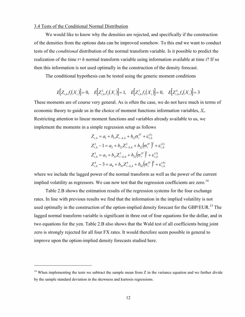
The conditional hypothesis can be tested using the generic moment conditions

( )[ ] ( )[ ] ( )[ ] ( )[ ] 3,0,1,0 44,3

3,2

2,1, ==== thtthtthttht XfZEXfZEXfZEXfZE

These moments are of course very general. As is often the case, we do not have much in terms of

economic theory to guide us in the choice of moment functions information variables, Xt.

Restricting attention to linear moment functions and variables already available to us, we

implement the moments in a simple regression setup as follows

( )( )

( ) )4(,

442

4,414

4,

)3(,

332

3,313

3,

)2(,

222

2,212

2,

)1(,12,111,

3

1

htIVthhtht

htIVthhtht

htIVthhtht

htIVthhtht

bZbaZ

bZbaZ

bZbaZ

bZbaZ

ε+σ++=−

ε+σ++=

ε+σ++=−

ε+σ++=

−

−

−

−

where we include the lagged power of the normal transform as well as the power of the current

implied volatility as regressors. We can now test that the regression coefficients are zero.14

Table 2.B shows the estimation results of the regression systems for the four exchange

rates. In line with previous results we find that the information in the implied volatility is not

used optimally in the construction of the option-implied density forecast for the GBP/EUR.15 The

lagged normal transform variable is significant in three out of four equations for the dollar, and in

two equations for the yen. Table 2.B also shows that the Wald test of all coefficients being joint

zero is strongly rejected for all four FX rates. It would therefore seem possible in general to

improve upon the option-implied density forecasts studied here.

14 When implementing the tests we subtract the sample mean from Z in the variance equation and we further divide

by the sample standard deviation in the skewness and kurtosis regressions.

13

3.5 Piecewise Density Evaluation

The inspection of the uniform histograms reveals that the densities have problems

particularly in the tails. In order formally test for misspecifications in the tail of the density

forecast we extend upon the testing methodology proposed by Berkowitz (2001).

Let a, b ∈ {0, 1} with a ≤ b. From the properties of the uniform distribution it follows that

if the density forecast is well specified then the collection of Ut,h ∈ {a, b} will be uniformly

distributed on {a, b} as well. We can than define another random variable Yt,h = (Ut,h-a)/(b-a)

with Ut,h ∈ {a, b} which is uniformly distributed on the interval {0, 1}. We can then use the

inverse normal transformation again to test for the specification of the density forecast in the

{a,b} interval.

The condition that Yt,h is uniformly distributed is necessary but not sufficient. For instance,

Ut,h could be uniformly distributed on a particular subset {a, b} of the interval {0, 1} but there

could still be too few or too many observations falling in the interval {a, b}. A further necessary

condition is that the coverage is correct. This corresponds to the requirement that the proportion

of the observations falling in the {a, b} interval is equal to b-a.

This requirement can be translated into a condition, which can be tested in a GMM

framework in addition to moment tests for the normality of ( )htht YZ ,1

,−Φ= . To do so we define

1 if0, if not

t ht,h

, U {a,b}I + ∈

=

And consider the following moments

( ) ( )( ) ( )

2, 1 , 2

3 4, 3 , 4

,

0, 1

0, 3

t h t t h t

t h t t h t

t h

E Z f X E Z f X

E Z f X E Z f X

E I b a

= = = = = −

Choosing particular moment functions and variables these conditions can be implemented in a

regression system setup as follows. For the unconditional case we have

15 Sub-sample tests not reported here reveals that the full sample rejection of the GBP forecasts is largely due to

problems early in the sample.

14

)5(,

5

5,

)4(,4

4,

)3(,3

3,

)2(,2

2,

)1(,1,

)exp(1)exp(

3

1

htht

htht

htht

htht

htht

aa

I

aZ

aZ

aZ

aZ

ε++

=

ε+=−

ε+=

ε+=−

ε+=

The estimation of the GMM system is done in such way as to specify the last condition as a

logistic regression. The joint null hypothesis can be tested with a Wald test that a1 = a2 = a3=a4

=0, and )()exp(1/()exp( 55 abaa −=+ . The conditional test mirrors exactly the test for the entire

distribution with the only addition of the fifth equation.

We implement the test on three subsets that are particularly relevant to our investigation:

the left tail, up to a theoretical probability mass of .25, the center of the distribution, from .25 to

.75, with a theoretical mass of .5, and the right tail with a theoretical mass of .25. The results are

reported in Tables 3-5. The Wald test results confirm that the tails are misspecified across the

board for all the densities, although for different reasons. The results do vary somewhat across

currencies for the center of the distribution. The conditional test cannot reject that the center of

the distribution is well specified for the USD/EUR and JPY/USD.

4. Interval Forecast Evaluation

Berkowitz (2001) has recently argued that it is possible that a density forecast may be

rejected overall even if it would provide adequate forecasts for certain segments of the

conditional distribution that are of particular interest to the forecaster. In this section we pursue

this issue via the construction of interval forecasts from the density forecasts from Section 3.

Interval forecasts and the closely related Value-at-Risk forecasts (one-sided interval forecasts)

have recently received much interest among financial practitioners as measures of portfolio risk.

They are therefore interesting in their own right.

In this section we study the performance of one-month interval forecasts calculated from

option prices and FX rates. The interval forecasts are constructed from the one-month option-

implied densities which in turn are calculated using the estimation method in Malz (1997) as

described in Section 3 above. We have computed conditional interval forecasts for the {0.45,

0.55} probability interval, as well as the {0.35, 0.65}, {0.25, 0.75}, {0.15, 0.85}, and the {0.05,

0.95} intervals. We now set out to evaluate the accuracy of the interval forecasts. To this end

15

consider the following simple framework based on Christoffersen (1998). Let the generic interval

forecast be defined as

{ })(),( , UhtLt,h pUpL

where pL and pU are the percentages associated with the lower and upper conditional quantiles

making up the interval forecast.

Consider now the indicator variable defined as

∈

= +

not if ,1if 0 )}(p),U(p{L S,

I Ut,hLt,hhtt,h

Then if the interval forecast is correctly calibrated, we must have that

( ) ( ) pppXI LUtht ≡−−== 1|1Pr ,

where Xt denotes a vector of information variables (and functions thereof) available on day t. If

the interval forecast is correctly calibrated then the expected outcome of the future FX rate falling

outside the predicted interval must be a constant equal to the pre-specified interval probability p.

This hypothesis will be tested in a logit regression setup. Under the alternative hypothesis

we have

( ) ( )( )t

ttht bXa

bXaXI

+++

==exp1

exp|1Pr ,

and the null hypothesis corresponds to the restrictions

( ))1/(ln,0 ppab −== .

Running these logit regressions on daily data we again have to worry about overlapping

observations, which we allow for using GMM estimation.

Table 6 shows the results for the logit regression tests of the interval forecasts. The interval

forecasts for the {0.45, 0.55}, {0.35, 0.65}, {0.25, 0.75}, {0.15, 0.85}, and the {0.05, 0.95}

intervals are denoted by the probability of an observation outside the interval, i.e. p=.90, .70, .50,

.30 and .10 respectively. We refer to these outside observations as hits. The zero/one hit sequence

is regressed on a constant, the 21-day lagged hit and the 21-day lagged 1-month implied

volatility. The lagged hit is included to capture any dependence in the outside observations. The

implied volatility is included to assess if it is incorporated optimally in the construction of the

interval forecast. If the interval forecast is correctly specified then the intercept should be ln(p/(1-

p)) and slopes should all be equal to zero. Table 6 reports coefficient estimates along with t-

statistics again calculated using GMM. Rather than reporting the constant term a, we report a’=a -

ln(p/(1-p)) and the t-stat for the test that a’=0. Below the solid line in each subsection of the table

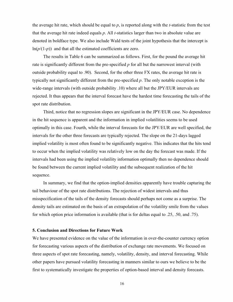
16

the average hit rate, which should be equal to p, is reported along with the t-statistic from the test

that the average hit rate indeed equals p. All t-statistics larger than two in absolute value are

denoted in boldface type. We also include Wald tests of the joint hypothesis that the intercept is

ln(p/(1-p)) and that all the estimated coefficients are zero.

The results in Table 6 can be summarized as follows. First, for the pound the average hit

rate is significantly different from the pre-specified p for all but the narrowest interval (with

outside probability equal to .90). Second, for the other three FX rates, the average hit rate is

typically not significantly different from the pre-specified p. The only notable exception is the

wide-range intervals (with outside probability .10) where all but the JPY/EUR intervals are

rejected. It thus appears that the interval forecast have the hardest time forecasting the tails of the

spot rate distribution.

Third, notice that no regression slopes are significant in the JPY/EUR case. No dependence

in the hit sequence is apparent and the information in implied volatilities seems to be used

optimally in this case. Fourth, while the interval forecasts for the JPY/EUR are well specified, the

intervals for the other three forecasts are typically rejected. The slope on the 21-days lagged

implied volatility is most often found to be significantly negative. This indicates that the hits tend

to occur when the implied volatility was relatively low on the day the forecast was made. If the

intervals had been using the implied volatility information optimally then no dependence should

be found between the current implied volatility and the subsequent realization of the hit

sequence.

In summary, we find that the option-implied densities apparently have trouble capturing the

tail behaviour of the spot rate distributions. The rejection of widest intervals and thus

misspecification of the tails of the density forecasts should perhaps not come as a surprise. The

density tails are estimated on the basis of an extrapolation of the volatility smile from the values

for which option price information is available (that is for deltas equal to .25, .50, and .75).

5. Conclusion and Directions for Future Work

We have presented evidence on the value of the information in over-the-counter currency option

for forecasting various aspects of the distribution of exchange rate movements. We focused on

three aspects of spot rate forecasting, namely, volatility, density, and interval forecasting. While

other papers have pursued volatility forecasting in manners similar to ours we believe to be the

first to systematically investigate the properties of option-based interval and density forecasts.

17

Our other findings can be summarized as follows. First, the implied volatilities from

currency options typically offer predictions that are unbiased and that explain more of the

variation in realized volatility than do volatility forecasts based on historical returns only.

Second, when evaluating the entire implied density forecasts these are generally rejected. Tests of

subsets of the density range suggest that the tails in the distribution are often misspecified. Third,

the option-implied intervals are accurate for the JPY/EUR but rejected for the other three

currencies in the study. We thus conclude that the information implied in option pricing is helpful

for volatility forecasting and for density and interval forecasting as long as the interest is

confined to the middle 70% range of the distribution.

The rejection of the widest intervals and the complete density forecast is of course

interesting and warrants further scrutiny. The potential reasons are at least fourfold. First, the

option contracts used may not have extreme enough strike prices to be useful for constructing

accurate distribution tails. Second, the information in options could be used sub-optimally in the

density estimates. Third, we could be rejecting the densities because certain information available

at the time of the forecasts is not incorporated in the option prices used to construct the densities,

i.e. option market inefficiencies. Fourth, the risk premium considerations, which were abstracted

from in this paper could be important enough to reject the risk-neutral density forecasts

considered. The misspecification of the mean in the case of the JPY/EUR rate suggests that an

omitted risk premium could be the culprit in that case. For the other three currencies, however,

the culprit appears to be tail misspecification, which is likely to arise from the lack of information

on deep in-the-money and deep out-of-the-money options.

Our results suggest several promising venues for future research. First, policy makers may

be interested in assessing speculative pressures on a given exchange rate. The option implied

densities can be used in this regard by constructing daily option-implied probabilities of say a 3%

appreciation or depreciation during the next month. Second, the accuracy of the left and right tail

interval forecast could be analyzed separately in order to gain further insight on the probability of

a sizable appreciation or depreciation. Third, relying on the triangular arbitrage condition linking

the JPY/EUR, the USD/EUR, and the JPY/USD, one can construct option implied covariances

and correlations from the option implied volatilities. These implied covariances can then be used

to forecast realized covariances as done for volatilities in this paper. Fourth, the misspecification

found in the option-implied density forecasts may be rectified by assuming different tail-shapes

in the density estimation or by incorporating return-based information. Converting the risk-

neutral densities to their statistical counterparts may improve the forecasts as well but will require

18

further assumptions, which may or may not be empirically valid. Bliss and Panigirtzoglou (2004)

present promising results in this direction.

19

References Ait-Sahalia, Y. and J. Duarte, 2003, Nonparametric Option Pricing under Shape Restrictions, Journal of Econometrics, 116, 9-47. Andersen, T., T. Bollerslev, F. X. Diebold, and P. Labys, 2003, Modeling and Forecasting Realized Volatility, Econometrica 71, 579-626. Baillie, R.T. and T. Bollerslev, 1989, The Message in Daily Exchange Rates: A Conditional-Variance Tale, Journal of Business & Economic Statistics, American Statistical Association, 7, 297-305. Bandi, F., and B. Perron, 2003, Long memory and the relation between implied and realized volatility, Manuscript, University of Chicago. Bank for International Settlements, 2003, Annual Report, Basle, Switzerland. Bank of England, 2000, Quarterly Bulletin, February, London. Bates, D., 2003 Empirical Option Pricing: A Retrospection," Journal of Econometrics 116:1/2, September/October, 387-404. Beckers, S., 1981, Standard deviations implied in options prices as predictors of future stock price volatility, Journal of Banking and Finance 5, 363-81. Benzoni, L. 2001, Pricing Options under Stochastic Volatility: An Empirical Investigation, Working Paper, University of Minnesota. Berkowitz, J., 2001, Testing Density Forecasts with Applications to Risk Management, Journal of Business and Economic Statistics 19, 465-474. Blair, B., S.-H. Poon, and S. Taylor, 2001, Forecasting S&P 100 volatility: The incremental information content of implied volatilities and high-frequency index returns, Journal of Econometrics 105, 5–26. Bliss, R. and N. Panigirtzoglou, 2004, Option-Implied Risk Aversion Estimates, Journal of Finance 59, 407-446. Bollerslev, T., and H. Zhou, 2005, Volatility Puzzles: A Unified Framework for Gauging Return-volatility Regressions, Journal of Econometrics, forthcoming. Bontemps, C., and N. Meddahi, 2005, Testing Normality: A GMM Approach, Journal of Econometrics, forthcoming. Breeden, D. and R. Litzenberger, H., 1978, Prices of state-contingent claims implicit in option prices, Journal of Business 51, 621-651 Canina, L., and S. Figlewski, 1993, The informational content of implied volatility, Review of Financial Studies 6, 659-81.

20

Chernov, M., 2003, On the role of volatility risk premia in implied volatilities based forecasting regressions, Manuscript, Columbia University. Christensen, B. J., and N.R. Prabhala, 1998, The relation between implied and realized volatility, Journal of Financial Economics 50, 125-50. Christoffersen P., 1998, Evaluating Interval Forecasts, International Economic Review 39, 841-862 Covrig, V. and B. S. Low, 2003, The Quality of Volatility Traded on the Over-the-Counter Currency Market: A Multiple Horizons Study, Journal of Futures Markets 23, 261-285. Diebold, F.X., T. Gunther, and A. S. Tay, 1998, Evaluating Density Forecasts with Applications to Financial Risk Management, International Economic Review 39, 863-883. Diebold, F.X., J. Hahn, and A. S. Tay, 1999, Multivariate Density Forecast Evaluation and Calibration in Financial Risk Management: High Frequency Returns on Foreign Exchange, Review of Economics and Statistics 81, 661-673 Fleming, J., 1998, The quality of market volatility forecasts implied by S&P 100 index option prices, Journal of Empirical Finance 5, 317-45. International Monetary Fund, 2002, Global Financial Stability Report, Washington, DC. Ioffe, I., 2004, Arbitrage Violations and Implied Valuations: The Option Market, Manuscript, Department of Finance, University of Minnesota. Jorion, P., 1995, Predicting Volatility in the Foreign Exchange Market, Journal of Finance 50, 507-528. Lamoureux, C., and W. Lastrapes, 1993, Forecasting stock-return variance: Toward an understanding of stochastic implied volatilities, Review of Financial Studies 6, 293-326. Malz, A., 1997, Estimating the Probability Distribution of the Future Exchange Rate from Option Prices, Journal of Derivatives, Winter, 18-36. Mincer, J. and V. Zarnowitz, 1969, The Evaluation of Economic Forecasts in J. Mincer (ed.), Economic Forecasts and Expectations, NBER, New York. Neely, C., 2003, Forecasting Foreign Exchange Volatility: Is Implied Volatility the Best We Can Do? Manuscript, Federal Reserve Bank of St. Louis. OECD, 1999, The Use of Financial Market Indicators by Monetary Authorities, Paris. Pong, S.-Y., M. Shackleton, S. J. Taylor, and X. Xu, 2004, Forecasting Currency Volatility: A Comparison of Implied Volatilities and AR(FI)MA Models, Journal of Banking and Finance 28, 2541-2563.

21

USD MSE Bias2 Inefficiency Random MSE Bias2 Inefficiency RandomImplied 7.99 1.25 3.16 95.58 6.46 1.43 5.80 92.77

Historical 12.08 0.00 27.19 72.81 9.16 0.05 28.80 71.15RiskMetrics 10.47 0.12 18.18 81.69 9.34 0.00 33.43 66.57

GARCH 9.04 2.80 1.96 95.24 6.34 1.24 1.91 96.85

JPY MSE Bias2 Inefficiency Random MSE Bias2 Inefficiency RandomImplied 14.42 1.29 0.76 97.94 11.20 0.49 0.51 99.01


GARCH 17.51 0.01 12.54 87.45 15.98 1.81 21.86 76.33

GBP MSE Bias2 Inefficiency Random MSE Bias2 Inefficiency RandomImplied 6.09 2.45 5.38 92.16 5.92 0.29 14.78 84.93


GARCH 7.66 0.02 13.68 86.30 7.29 1.11 26.70 72.19

JPY/USD MSE Bias2 Inefficiency Random MSE Bias2 Inefficiency RandomImplied 14.89 2.31 0.93 96.75 12.19 2.56 1.67 95.77


GARCH 15.66 1.56 1.21 97.23 12.78 2.72 0.55 96.73

Table 1: MSE and Mincer-Zarnowitz percentage decomposition

1-Month 3-Month

Notes to table: For each exchange rate and forecast horizon we regress realized volatility on each

volatility forecast and compute the mean squared error (MSE) from the regression. The table

reports the MSE along with the percentage Mincer-Zarnowitz decomposition into squared bias,

inefficiency and random variation.

22

Estimate t-stat Estimate t-stat Estimate t-stat Estimate t-statMean 0.072 1.018 -0.297 -4.031 -0.024 -0.278 -0.040 -0.525Var -0.201 -3.284 -0.070 -0.809 0.343 2.244 -0.073 -0.838Skew 0.163 0.732 -0.033 -0.120 0.490 1.511 -0.359 -1.243Kurt -0.299 -0.727 0.180 0.297 1.153 1.247 0.031 0.043

Stats p-val Stats p-val Stats p-val Stats p-valWald-test 50.6 0.000 64.0 0.000 29.6 0.000 7.5 0.112

Estimate t-stat Estimate t-stat Estimate t-stat Estimate t-statConst 0.621 1.962 -0.346 -1.271 0.780 2.762 -0.088 -0.307Lag LHS 0.128 2.295 0.145 2.573 0.304 4.328 0.120 1.9111MIV(-21) -0.050 -1.861 0.010 0.448 -0.095 -3.115 0.006 0.247

Const 0.030 0.197 0.128 0.726 0.854 3.635 0.160 0.929Lag LHS -0.122 -3.540 -0.023 -0.463 0.332 3.150 -0.011 -0.2661MIV(-21)2 -0.002 -2.046 -0.001 -1.154 -0.009 -4.003 -0.002 -1.751

Const 0.605 1.563 -0.239 -0.680 0.860 2.083 -0.365 -0.956Lag LHS 0.021 0.911 0.093 2.185 0.328 2.665 0.068 2.2391MIV(-21)3 0.000 -1.674 0.000 1.069 -0.001 -2.258 0.000 0.413

Const 0.165 0.279 0.334 0.610 1.675 1.861 0.170 0.214Lag LHS -0.047 -2.084 -0.001 -0.048 0.312 2.152 -0.014 -0.8331MIV(-21)4 0.000 -1.815 0.000 -0.541 0.000 -2.710 0.000 -1.208


Table 2.B: Conditional Test of Normal Transform

USD JPY GBP JPY/USD

Table 2.A: Unconditional Test of Normal Transform

USD JPY GBP JPY/USD

Notes to table: For each exchange rate density forecast we construct the normal transform

variable and test the first four unconditional moments in Panel A. In Panel B we regress powers

of the normal transform variable on its lag and powers of implied volatility to test the conditional

moments. The joint moment hypotheses are assessed in the Wald tests.

23

Estimate t-stat Estimate t-stat Estimate t-stat Estimate t-statMean 0.301 3.831 -0.036 -0.421 -0.025 -0.262 0.015 0.140Var -0.292 -4.780 0.055 0.475 0.089 0.629 0.069 0.413Skew 0.143 0.522 -0.219 -0.714 -0.451 -1.229 -0.359 -0.813Kurt -0.235 -0.566 0.345 0.508 0.401 0.473 0.558 0.543

Estimate p-val Estimate p-val Estimate p-val Estimate p-valCoverage 0.217 0.000 0.357 0.000 0.287 0.000 0.264 0.000


Estimate t-stat Estimate t-stat Estimate t-stat Estimate t-statConst -0.351 -0.801 -0.578 -1.074 -0.692 -1.270 0.581 0.657Lag LHS -0.144 -1.574 -0.035 -0.415 0.242 3.204 0.003 0.0261MIV(-21) 0.083 2.153 0.045 1.030 0.053 0.961 -0.052 -0.576

Const -0.484 -2.445 0.679 1.542 0.941 1.116 -0.763 -1.968Lag LHS -0.164 -1.259 -0.012 -0.164 -0.009 -0.115 -0.011 -0.1711MIV(-21)2 0.002 0.968 -0.005 -2.029 -0.008 -1.059 0.006 2.040

Const -0.057 -0.103 -1.121 -1.170 -2.166 -1.304 -0.175 -0.205Lag LHS 0.033 0.219 -0.061 -1.323 0.060 0.914 -0.030 -0.7611MIV(-21)3 0.001 3.140 0.000 1.145 0.001 0.995 0.000 -0.306

Const -0.249 -0.309 2.092 1.154 4.185 1.164 -1.189 -0.785Lag LHS -0.002 -0.015 -0.029 -0.768 -0.038 -0.691 -0.027 -0.7831MIV(-21)4 0.000 1.541 0.000 -2.031 0.000 -1.328 0.000 1.340



USD JPY GBP JPY/USD

Table 3.B: Conditional Test of the Normal Transform for {a,b} = {0,.25}

Table 3.A: Unconditional Test of the Normal Transform for {a,b} = {0,.25}

USD JPY GBP JPY/USD


variable for the left tail and test the first four unconditional moments in Panel A. In Panel B we

regress powers of the normal transform variable on its lag and powers of implied volatility to test

the conditional moments.

24

Estimate t-stat Estimate t-stat Estimate t-stat Estimate t-statMean -0.055 -0.979 -0.137 -2.375 -0.189 -2.934 0.024 0.413Var -0.066 -1.445 0.050 0.900 0.034 0.535 0.072 1.314Skew 0.142 0.801 0.188 1.139 0.061 0.340 0.058 0.357Kurt 0.223 0.580 0.061 0.190 -0.031 -0.094 -0.102 -0.339



Estimate t-stat Estimate t-stat Estimate t-stat Estimate t-statConst 0.080 0.201 0.315 1.182 0.499 1.292 0.374 1.361Lag LHS -0.005 -0.098 -0.063 -0.924 0.050 0.906 -0.093 -1.5981MIV(-21) -0.012 -0.377 -0.036 -1.623 -0.098 -2.350 -0.026 -1.235

Const 0.004 0.023 -0.322 -2.130 0.350 1.910 0.280 1.866Lag LHS -0.033 -1.237 0.053 0.889 0.001 0.022 0.060 1.4351MIV(-21)2 0.000 -0.394 0.003 2.713 -0.002 -1.487 -0.001 -1.204

Const 0.279 0.714 0.613 2.169 0.100 0.241 0.269 1.012Lag LHS 0.010 0.428 -0.009 -0.126 0.033 0.728 -0.041 -0.9241MIV(-21)3 0.000 -0.875 0.000 -1.655 -0.001 -1.683 0.000 -1.615

Const 0.010 0.018 -0.530 -0.962 0.826 1.443 0.440 0.859Lag LHS -0.031 -2.251 0.072 0.933 -0.010 -0.271 0.014 0.7641MIV(-21)4 0.000 0.074 0.000 1.785 0.000 -1.862 0.000 -1.165



USD JPY GBP JPY/USD

USD JPY GBP JPY/USD

Table 4.A: Unconditional Test of the Normal Transform for {a,b} = {.25,.75}

Table 4.B: Conditional Test of the Normal Transform for {a,b} = {0.25,.75}


variable for the center of the distribution and test the first four unconditional moments in Panel

A. In Panel B we regress powers of the normal transform variable on its lag and powers of

implied volatility to test the conditional moments.

25

Estimate t-stat Estimate t-stat Estimate t-stat Estimate t-statMean -0.075 -0.978 -0.212 -1.893 0.256 1.844 -0.280 -3.476Var -0.205 -2.610 -0.231 -1.755 0.637 2.504 -0.309 -4.462Skew 0.010 0.036 0.403 0.866 0.729 1.791 -0.213 -0.633Kurt 0.306 0.462 -0.129 -0.125 0.663 0.761 0.232 0.394



Estimate t-stat Estimate t-stat Estimate t-stat Estimate t-statConst 0.455 0.845 -1.667 -1.818 1.245 2.968 0.205 0.258Lag LHS -0.221 -2.937 0.031 0.163 0.377 2.264 0.103 1.0211MIV(-21) -0.051 -0.931 0.149 1.608 -0.122 -2.078 -0.022 -0.275

Const -0.578 -3.380 -1.035 -1.845 1.171 2.377 -0.394 -0.891Lag LHS 0.010 0.193 0.018 0.150 0.298 1.603 -0.137 -1.6741MIV(-21)2 0.003 2.281 0.010 1.690 -0.003 -0.556 0.003 0.827

Const 0.127 0.233 -2.203 -1.790 1.989 2.977 0.338 0.247Lag LHS -0.072 -0.982 -0.093 -0.623 0.431 2.067 0.000 -0.0051MIV(-21)3 0.000 -0.515 0.002 1.870 -0.001 -2.054 0.001 0.426

Const -0.307 -0.332 -4.195 -2.108 3.140 2.147 0.228 0.127Lag LHS 0.018 0.726 -0.038 -0.267 0.331 1.396 -0.104 -1.6931MIV(-21)4 0.000 0.969 0.000 1.908 0.000 -1.885 0.000 1.122



USD JPY GBP JPY/USD

USD JPY GBP JPY/USD

Table 5.A: Unconditional Test of the Normal Transform for {a,b} = {.75,1}

Table 5.B: Conditional Test of the Normal Transform for {a,b} = {0.75,1}


variable for the right tail and test the first four unconditional moments in Panel A. In Panel B we

regress powers of the normal transform variable on its lag and powers of implied volatility to test

the conditional moments.

26

Figure 1: Histogram of Probability Transforms with 90% Confidence Band

0 0.5 10

50

100

150

200USD

0 0.5 10

50

100

150

200JPY

0 0.5 10

50

100

150

200GBP

0 0.5 10

50

100

150

200JPY/USD

Notes to figure: For each exchange rate we plot the histogram of the probability transform

variable from the option implied density forecasts. The horizontal lines denote the 90%

confidence interval that the transform variables are uniformly distributed.

27

Figure 2: Histogram of Normal Transforms with Normal Distribution Imposed

-5 0 50

100

200

300USD

-5 0 50

100

200

300JPY

-5 0 50

100

200

300GBP

-5 0 50

100

200

300JPY/USD

Notes to figure: For each exchange rate we plot the histogram of the normal transform variable

from the option implied density forecasts. Each histogram is superimposed on a normal density

function.

28

Figure 3: QQ Plots of Normal Transform Variables

-4 -2 0 2 4-4

-2

0

2

4USD

-4 -2 0 2 4-4

-2

0

2

4JPY

-4 -2 0 2 4-4

-2

0

2

4

6GBP

-4 -2 0 2 4-4

-2

0

2

4JPY/USD

Notes to figure: For each exchange rate we scatter plot the empirical quantile of the normal

transform variable from the option implied density forecast against the corresponding quantile of

the normal distribution. The diagonal line denotes a perfect fit.

29

APPENDIX

USD/DEM JPY/DEM GBP/DEM JPY/USD USD/DEM JPY/DEM GBP/DEM JPY/USD Mean -8.25E-05 -4.11E-05 2.21E-05 -3.57E-05 5.07E-05 5.35E-05 2.89E-05 6.21E-05 Std. Dev. 7.12E-03 7.32E-03 5.38E-03 7.88E-03 1.03E-04 1.64E-04 8.33E-05 1.96E-04 Skewness -0.110 -0.876 0.653 -0.855 6.129 11.998 20.852 14.721 Kurtosis 5.084 10.346 9.267 10.962 57.905 194.273 634.957 328.912 Jarque-Bera 306 3783 2836 4615 220218 2465015 27760096 7451371 Observations 1670 1592 1661 1670 1670 1592 1661 1670

USD/DEM JPY/DEM GBP/DEM USD/DEM JPY/DEM GBP/DEMJPY/DEM 0.301 JPY/DEM 0.155GBP/DEM 0.348 0.087 GBP/DEM 0.124 0.073JPY/USD -0.467 0.228 -0.203 JPY/USD 0.215 0.326 0.045

USD/EUR JPY/EUR GBP/EUR JPY/USD USD/EUR JPY/EUR GBP/EUR JPY/USD Mean -1.41E-04 -1.18E-04 -1.17E-04 2.24E-05 4.79E-05 7.07E-05 2.54E-05 4.43E-05 Std. Dev. 6.92E-03 8.41E-03 5.04E-03 6.66E-03 8.93E-05 1.60E-04 4.64E-05 8.39E-05 Skewness 0.422 0.046 0.347 -0.149 8.472 8.871 4.300 4.836 Kurtosis 4.512 6.107 4.379 4.581 139.912 128.608 28.362 35.773 Jarque-Bera 129 415 102 111 816790 690618 30778 50109 Observations 1030 1030 1030 1030 1030 1030 1030 1030

USD/EUR JPY/EUR GBP/EUR USD/EUR JPY/EUR GBP/EURJPY/EUR 0.638 JPY/EUR 0.610GBP/EUR 0.704 0.487 GBP/EUR 0.421 0.212JPY/USD -0.234 0.600 -0.117 JPY/USD 0.134 0.488 0.011

Squared Daily ReturnsDaily Returns

Table A.2: Foreign Exchange Descriptive statistics. Post 1999

Table A.1: Foreign Exchange Descriptive statistics. Pre 1999

Squared Daily Returns Pairwise CorrelationsDaily Returns Pairwise Correlations

Daily Returns Squared Daily Returns

Squared Daily Returns Pairwise CorrelationsDaily Returns Pairwise Correlations

Notes to tables: Descriptive statistics are calculated for daily FX returns and squared returns.

Prior to 1999 exchange rates are quoted against the DEM (except for the JPY/USD) and post

1999 exchange rates are quoted against the EUR.

30

1-M IV 3-M IV 1-M HV 3-M HV 1-M GARCH 3-M GARCH RM Mean 10.94 11.07 10.69 10.90 11.17 11.06 10.81

Std. Dev. 2.34 1.88 3.36 2.72 2.01 1.60 3.00 Skewness 0.90 0.44 1.29 0.94 1.43 1.29 1.18 Kurtosis 4.59 3.03 5.19 3.76 6.59 6.42 4.82

Jarque-Bera 662.1 87.1 1378.7 497.7 2545.0 2207.6 1072.3 Observations 2748 2748 2893 2893 2893 2893 2893





Std. Dev. 2.28 1.91 2.97 2.48 2.45 2.27 2.71 Skewness 0.35 -0.07 1.68 1.03 2.20 2.34 1.42 Kurtosis 3.21 2.85 8.99 4.80 13.35 14.99 7.05





JPY/USD

Table A.3: Foreign Exchange Volatility: Descriptive statistics

USD

JPY

GBP

Notes to Table: For each exchange rate we compute the descriptive statistics for the various

annualized 1-month and 3-month volatility forecasts analyzed in Section 2. The forecasts are:

Implied Volatility (IV), Historical Volatility (HV), GARCH, and RiskMetrics (RM). For

RiskMetrics the forecast is the same for both horizons. The sample period is March 31, 1992 –

February 19, 2003.

31

IV RV HV GARCH IV RV HV GARCH RV 0.554 RV 0.459 HV 0.790 0.452 HV 0.818 0.376

GARCH 0.793 0.471 0.915 GARCH 0.723 0.437 0.753RM 0.844 0.473 0.945 0.922 RM 0.797 0.424 0.869 0.903

IV RV HV GARCH IV RV HV GARCH

RV 0.609 RV 0.591 HV 0.821 0.558 HV 0.866 0.572

GARCH 0.845 0.567 0.943 GARCH 0.798 0.537 0.792RM 0.871 0.571 0.952 0.951 RM 0.837 0.571 0.892 0.926


GARCH 0.780 0.498 0.915 GARCH 0.699 0.374 0.684RM 0.847 0.484 0.956 0.894 RM 0.791 0.390 0.879 0.888


GARCH 0.789 0.605 0.908 GARCH 0.691 0.549 0.741RM 0.837 0.619 0.960 0.905 RM 0.782 0.619 0.913 0.890

1-Month 3-Month

JPY/USD1-Month 3-Month

JPY1-Month 3-Month

GBP

Table A.4: Foreign Exchange Volatility Forecasts: Correlation

USD1-Month 3-Month

Notes to table: For each exchange rate and forecast horizon we compute the correlation matrix for

the four competing volatility forecasts considered in Section 2. The sample period is March 31,

1992 – February 19, 2003.

The Accuracy of Density Forecasts from Foreign...

Documents

Transcript of The Accuracy of Density Forecasts from Foreign...