Density Forecasts in Panel Data Models:

A Semiparametric Bayesian Perspective∗

Laura Liu†

University of Pennsylvania

April 28, 2017

Abstract

This paper constructs individual-specic density forecasts for a panel of rms or households

using a dynamic linear model with common and heterogeneous coecients and cross-sectional

heteroskedasticity. The panel considered in this paper features large cross-sectional dimension

(N) but short time series (T ). Due to short T , traditional methods have diculty in disentangling

the heterogeneous parameters from the shocks, which contaminates the estimates of the hetero-

geneous parameters. To tackle this problem, I assume that there is an underlying distribution

of heterogeneous parameters, model this distribution nonparametrically allowing for correlation

between heterogeneous parameters and initial conditions as well as individual-specic regressors,

and then estimate this distribution by pooling the information from the whole cross-section to-

gether. I develop a simulation-based posterior sampling algorithm specically addressing the

nonparametric density estimation of unobserved heterogeneous parameters. I prove that both

the estimated common parameters and the estimated distribution of the heterogeneous parame-

ters achieve posterior consistency, and that the density forecasts asymptotically converge to the

oracle forecast, an (infeasible) benchmark that is dened as the individual-specic posterior pre-

dictive distribution under the assumption that the common parameters and the distribution of

the heterogeneous parameters are known. Monte Carlo simulations demonstrate improvements

in density forecasts relative to alternative approaches. An application to young rm dynamics

also shows that the proposed predictor provides more accurate density predictions.

JEL Codes: C11, C14, C23, C53, L25

Keywords: Bayesian, Semiparametric Methods, Panel Data, Density Forecasts, Posterior

Consistency, Young Firms Dynamics

∗First version: November 15, 2016. Latest version: https://goo.gl/c6Ybrd. I am indebted to my advisors, FrancisX. Diebold and Frank Schorfheide, for much help and guidance at all stages of this research project. I also thank theother members of my committee, Xu Cheng and Francis J. DiTraglia, for their advice and support. I further benetedfrom many helpful discussions with Gianni G. Amisano, Evan Chan, Timothy Christensen, Benjamin Connault,Jeremy Greenwood, Hyungsik R. Moon, Andriy Norets, Paul Sangrey, Minchul Shin, Molin Zhong, and seminarparticipants at the University of Pennsylvania, the Federal Reserve Bank of Philadelphia, the Federal Reserve Board,the University of Virginia, Microsoft, the University of California, Berkeley, the University of California, San Diego(Rady), Boston University, and the University of Illinois at UrbanaChampaign, as well as conference participantsat the 26th Annual Meeting of the Midwest Econometrics Group. I would also like to acknowledge the KaumanFoundation and the NORC Data Enclave for providing researcher support and access to the condential microdata.All remaining errors are my own.†Department of Economics, University of Pennsylvania, Philadelphia, PA 19104. Email: yuliu4@sas.upenn.edu.

1 Introduction

Panel data, such as a collection of rms or households observed repeatedly for a number of periods,

are widely used in empirical studies and can be useful for forecasting individuals' future outcomes,

which is interesting and important in many applications. For example, PSID can be used to an-

alyze income dynamics (Hirano, 2002; Gu and Koenker, 2015), and bank balance sheet data can

help conduct bank stress tests (Liu et al., 2016). This paper constructs individual-specic density

forecasts using a dynamic linear panel data model with common and heterogeneous parameters and

cross-sectional heteroskedasticity.

In this paper, I consider young rm dynamics as the empirical application. For illustrative

purposes, let us consider a simple dynamic panel data model as the baseline setup:

yit︸︷︷︸performance

= βyi,t−1 + λi︸︷︷︸skill

+ uit︸︷︷︸shock

, uit ∼ N(0, σ2

), (1.1)

where i = 1, · · · , N , and t = 1, · · · , T + 1. The yit is the observed rm performance such as the

log of employment,1 λi is the unobserved skill of an individual rm, and uit is an i.i.d. shock. Skill

is independent of the shock, and the shock is independent across rms and times. β and σ2 are

common across rms, where β represents the persistence of the dynamic pattern, and σ2 gives the

size of the shocks. Based on the observed panel from period 0 to period T , I am interested in

forecasting the future performance of any specic rm in period T + 1, yi,T+1.

The panel considered in this paper features large cross-sectional dimension N but short time

series T . This framework is appealing to the young rm dynamics example because the number

of observations for each young rm is restricted by its age. Good estimates of the unobserved

skill λis facilitate good forecasts of yi,T+1s. Due to short T , traditional methods have diculty in

disentangling the unobserved skill λi from the shock uit, which contaminates the estimates of λi.

The naive estimators that only utilize the rm-specic observations are inconsistent even if N goes

to innity.

To tackle this problem, I assume that λi is drawn from the underlying skill distribution f and

estimate this distribution by pooling the information from the whole cross-section together. In terms

of modeling f , the parametric Gaussian density misses many features in real world data, such as

asymmetricity, heavy tails, and multiple peaks. For example, since good ideas are scarce, the skill

distribution of young rms may be highly skewed. In this sense, the challenge now is how we can

model f more carefully and exibly. Here I estimate f via a nonparametric Bayesian approach where

the prior is constructed from a mixture model and allows for correlation between λi and the initial

condition yi0 (i.e. a correlated random eects model).

Once this distribution is estimated, I can, intuitively speaking, use it as a prior distribution and

1Employment is one of the standard measures in the rm dynamics literature (Akcigit and Kerr, 2010; Zarutskieand Yang, 2015).

1

update it with the rm-specic data and obtain the rm-specic posterior. In a special case where

the common parameters are set to be β = 0 and σ2 = 1, the rm-specic posterior is characterized

by Bayes' theorem,

p (λi |f, yi,0:T ) =p (yi,1:T |λi) f (λi |yi0 )´p (yi,1:T |λi) f (λi |yi0 ) dλi

. (1.2)

This rm-specic posterior helps provide a better inference about the unobserved skill λi of each

individual rm and a better forecast of the rm-specic future performance, thanks to the underlying

distribution f that integrates the information from the whole panel in an ecient and exible way.2

It is natural to construct density forecasts based on the rm-specic posterior. In general,

forecasting can be done in point, interval, or density fashion, whereas density forecasts give the

richest insight regarding future outcomes. By denition, a density forecast provides a predictive

distribution of rm i's future performance and summarizes all sources of uncertainties, hence is

preferable in the context of young rm dynamics and other applications with large uncertainties

and nonstandard distributions. In particular, for the dynamic panel data model as specied in

equation (1.1), the density forecasts reect uncertainties arising from future shock ui,T+1, individual

heterogeneity λi, and estimation uncertainty of common parameters(β, σ2

)and skill distribution f .

A typical question that density forecasts could answer is: what is the chance that rm i will

hire 5, 10, or 100 more people next year? The answer to this kind of question is valuable to both

investors and regulators regarding how promising or troublesome each rm could be. For investors, it

is helpful to select a better performing portfolio of startups.3 For regulators, more accurate forecasts

facilitate monitoring and regulation of bank-lending practices and entrepreneur funding.4 Moreover,

once the density forecasts are obtained, one can easily recover the point and interval forecasts.

A benchmark for evaluating density forecasts is the posterior predictive distribution for yi,T+1

under the assumption that the common parameters(β, σ2

)and the distribution of the heterogeneous

coecients f are known. I refer to this predictive density as the (infeasible) oracle forecast. In the

special case where β = 0 and σ2 = 1, it is straightforward to construct the oracle predictor for rm

i, which combines rm i's uncertainties due to future shock and heterogeneous skill.

foraclei,T+1 (y) =

ˆφ (y − λi)︸ ︷︷ ︸future shock

· p (λi |f0, yi,0:T )︸ ︷︷ ︸heterogeneous skill

· dλi.

The part of skill uncertainty is exactly the rm-specic posterior in equation (1.2) and arises from

the lack of time-series information available to infer individual λi. Therefore, the common skill

2Note that this is only an intuitive explanation why the skill distribution f is crucial. In the actual implementation,the estimation of the correlated random eect distribution f , the estimation of common parameters

(β, σ2

), and the

inference of rm-specic skill λi are all done simultaneously.3The general model studied can include aggregate variables that have heterogeneous eects on individual rms,

so their coecients can be thought of as the betas for portfolio choices.4The aggregate-level forecasts can be obtained by summing rm-specic forecasts over dierent subgroups.

2

distribution f0 helps in formulating rm i's skill uncertainty and contributes to rm i's density

forecasts through the channel of skill uncertainty.

In practice, however, the skill distribution f (as well as the common parameters for models

beyond the special case) is unknown and unobservable, thus introducing another source of uncer-

tainty. Now the oracle predictor becomes an infeasible optimum. A good feasible predictor should

be as close to the oracle as possible, which in turn calls for a good estimate of the underlying skill

distribution f . The proposed semiparametric Bayesian procedure achieves better estimates of the

underlying skill distribution f than parametric approaches, hence more accurate density forecasts of

the future outcomes. In the special case where β = 0 and σ2 = 1, the three sources of uncertainties

can be decomposed as follows:5

fspi,T+1 (y) =

ˆφ (y − λi)︸ ︷︷ ︸future shock

· p (λi |f, yi,0:T )︸ ︷︷ ︸heterogeneous skill

· dΠ (f |y1:N,0:T )︸ ︷︷ ︸estimation

dλi.

The contributions of this paper are threefold. First, I develop a posterior sampling algorithm

specically addressing nonparametric density estimation of the unobserved λi. For a random eects

model, which is a special case with zero correlation between λi and yi0, the f part becomes a

relatively simple unconditional density estimation problem. I impose a Dirichlet Process Mixture

(DPM) prior on f and construct a posterior sampler building on the blocked Gibbs sampler proposed

by Ishwaran and James (2001, 2002). For a correlated random eects model, I further adapt the

proposed algorithm to the much harder conditional density estimation problem using a probit stick

breaking process prior suggested by Pati et al. (2013).

Second, I establish the theoretical properties of the proposed semiparametric Bayesian predictor

when the cross-sectional dimensionN tends to innity. First, I provide conditions for identifying both

the parametric component(β, σ2

)and the nonparametric component f . Second, I prove that both

the estimated common parameters and the estimated distribution of the heterogeneous coecients

achieve posterior consistency, an essential building block for bounding the discrepancy between the

proposed predictor and the oracle. Compared to previous literature on posterior consistency, there

are several challenges in the current setting: (1) disentangling unobserved individual eects λis and

shocks uits, (2) incorporating an unknown shock size σ2, (3) adding lagged dependent variables as

covariates, and (4) addressing correlated random eects from a conditional density estimation point

of view. Finally, I show that the density forecasts asymptotically converge to the oracle forecast in

weak topology, which constitutes another contribution to the nonparametric Bayesian literature and

specically designed for density forecasts.

To accommodate many important features of real-world empirical studies, I extend the simple

model (1.1) to a more general specication. First, a realistic application also incorporates other

observables with common eects (β′xi,t−1), where xi,t−1 can include lagged yit. Second, it is helpful to

5The superscript sp stands for semiparametric.

3

consider observables with heterogeneous eects (λ′iwi,t−1), i.e. a correlated random coecients model.

Finally, beyond heterogeneity in coecients (λi), it is desirable to take into account heterogeneity in

shock sizes (σ2i ) as well.

6 All numerical methods and theoretical properties are further established

for the general specication.

Third, Monte Carlo simulations demonstrate improvements in density forecasts relative to pre-

dictors with various parametric priors on f , evaluated by log predictive score. An application

to young rm dynamics also shows that the proposed predictor provides more accurate density

predictions. The better forecasting performance is largely due to three key features (in order of

importance): the nonparametric Bayesian prior, cross-sectional heteroskedasticity, and correlated

random coecients. The estimated model also helps shed light on the latent heterogeneity structure

of rm-specic coecients and cross-sectional heteroskedasticity, as well as whether and how these

unobserved heterogeneous features depend on the initial condition of the rms.

It is worth mentioning that although I describe the econometric intuition using the young rm

dynamics application as an example, the method can be applied to many economic and nancial

analyses that feature panel data with relatively large N and small T , such as microeconomic panel

surveys (e.g. PSID, NLSY, and Consumer Expenditure Survey (CE)), macroeconomic sectoral and

regional panel data (e.g. Industrial Production (IP), and State and Metro Area Employment, Hours,

and Earnings (SAE)), and nancial institution performance (e.g. Commercial Bank Data and Hold-

ing Company Data). Which T can be considered as a small T depends on the dimension of individual

heterogeneity (dw), the cross-sectional dimension (N), and size of the shocks (σ2 or σ2i ). There can

still be a signicant gain in density forecasts even when T exceeds 100. Roughly speaking, the

proposed predictor would provide sizeable improvement as long as the time series for individual i is

not informative enough to fully reveal its individual eects, λi and σ2i .

Moreover, the method proposed in this paper is general to many other problems beyond fore-

casting. Here estimating heterogeneous parameters is important because we want to generate good

forecasts, but in other cases, the heterogeneous parameters themselves can possibly be the objects

of interest. For example, people may be interested in individual-specic treatment eects, and the

technique developed here can be applied to those questions.

Related Literature First, this paper contributes to the literature on individual forecast in a

panel data setup, and is closely related to Liu et al. (2016) and Gu and Koenker (2015, 2016). Liu

et al. (2016) focus on point forecasts. They utilize the idea of Tweedie's formula to steer away from

the complicated deconvolution problem in estimating λi. Unfortunately, the Tweedie shortcut is

not applicable to the inference of underlying λi distribution and therefore not suitable for density

forecasts.

6Here and below, the terminologies random eects model and correlated random eects model also apply toindividual eects on σ2

i , which are slightly dierent from the traditional denitions concentrated on λi.

4

Gu and Koenker (2015) address the density estimation problem. Their method is dierent from

the one proposed in this paper in that this paper infers the underlying λi distribution via a full

Bayesian approach (i.e. imposing a prior on the λi distribution and updating the prior belief by the

observed data), whereas they employ an empirical Bayes procedure (i.e. picking the λi distribution

by maximizing the marginal likelihood of data). In principle, the full Bayesian approach is prefer-

able for density forecasts as it captures all kinds of uncertainties, including estimation uncertainty

of the underlying λi distribution, which has been omitted by the empirical Bayes procedure. In ad-

dition, this paper features correlated random eects allowing for both cross-sectional heterogeneities

and cross-sectional heteroskedasticities interacting with the initial conditions, whereas the Gu and

Koenker (2015) approach focuses on random eects models without such interaction.

In their recent paper, Gu and Koenker (2016) also compare their method with an alternative

nonparametric Bayesian estimator featuring a Dirichlet Process (DP) prior under a set of xed scale

parameters. There are two major dierences between their DP setup and the DPM prior used in

this paper. First, the DPM prior provides continuous individual eect distributions, which is more

reasonable in many empirical setups. Second, unlike their set of xed scale parameters, this paper

incorporates a hyperprior for the scale parameter and updates it via the observed data, hence let

the data choose the complexity of the mixture approximation, which can essentially be viewed as

automatic model selection.7

There have also been empirical works on the DPM model with panel data, such as Hirano (2002),

Burda and Harding (2013), Rossi (2014), and Jensen et al. (2015), but they focus on empirical

studies rather than theoretical analysis. Hirano (2002) and Jensen et al. (2015) use linear panel

models, while their setups are slightly dierent from this paper. Hirano (2002) considers exibility

in uit distribution instead of λi distribution. Jensen et al. (2015) assume random eects instead of

correlated random eects. Burda and Harding (2013) and Rossi (2014) implement nonlinear panel

data models via either a probit model or a logit model, respectively.

Among others, Delaigle et al. (2008) have also studied the similar deconvolution problem and

estimated the λi distribution in a frequentist way, but the frequentist approach misses estimation

uncertainty, which matters in density forecasts, as mentioned previously.

Second, in terms of asymptotic properties, this paper relates to the literature on posterior con-

sistency of nonparametric Bayesian methods in density estimation problems. The pioneer work by

Schwartz (1965) lays out two high-level sucient conditions in a general density estimation context.

Ghosal et al. (1999) bring Schwartz (1965)'s idea into the analysis of density estimation with DPM

priors. Amewou-Atisso et al. (2003) extend the discussion to linear regression problems with an

unknown error distribution. Tokdar (2006) further generalizes the results to cases in which the true

density has heavy tails. For a more thorough review and discussion on posterior consistency in

Bayesian nonparametric problems, please refer to the handbooks, Ghosh and Ramamoorthi (2003)

7Section 6 shows the simulation results comparing the DP prior vs the DPM prior, where both incorporate ahyperprior for the scale parameter.

5

and Hjort et al. (2010) (especially Chapters 1 and 2). To handle conditional density estimation,

similar mixture structure can be implemented, where the mixing probabilities can be characterized

by a multinomial choice model (Norets, 2010; Norets and Pelenis, 2012), a kernel stick break process

(Norets and Pelenis, 2014; Pelenis, 2014), or a probit stick breaking process (Pati et al., 2013). I

adopt the Pati et al. (2013) approach to oer a more coherent nonparametric framework that is

totally exible in the conditional measure. This paper builds on these previous works and estab-

lishes the posterior consistency result for panel data models. Furthermore, this paper obtains the

convergence of the semiparametric Bayesian predictor to the oracle predictor, which is another new

nding to the literature and specic to density forecasts.

Third, the algorithms constructed in this paper build on the literature on the posterior sampling

schemes for DPM models. The vast Markov chain Monte Carlo (MCMC) algorithms can be divided

into two general categories. One is the Pólya urn style samplers that marginalize over the unknown

distribution G (Escobar and West, 1995; Neal, 2000).8 The other resorts to the stick breaking process

(Sethuraman, 1994) and directly incorporates G into the sampling procedure. This paper utilizes a

sampler from the second category, Ishwaran and James (2001, 2002)'s blocked Gibbs sampler, as a

building block for the proposed algorithm. Basically, it incorporates truncation approximation and

augments the data with auxiliary component probabilities, which helps break down the complex

posterior structure and thus enhance mixing properties as well as reduce computation time.9 I

further adapt the proposed algorithm to the conditional density estimation for correlated random

eects using the probit stick breaking process prior suggested by Pati et al. (2013).

Last but not least, the empirical application in this paper also links to the young rm dynamics

literature. Akcigit and Kerr (2010) document the fact that R&D intensive rms grow faster, and

such boosting eects are more prominent for smaller rms. Robb and Seamans (2014) examine the

role of R&D in capital structure and performance of young rms. Zarutskie and Yang (2015) present

some empirical evidence that young rms experienced sizable setbacks during the recent recession,

which may partly account for the slow and jobless recovery. For a thorough review on young rm

innovation, please refer to the handbook by Hall and Rosenberg (2010). The empirical analysis of this

paper builds on these previous ndings. Besides providing more accurate density forecasts, we can

also use the estimated model to analyze the latent heterogeneity structure of rm-specic coecients

and cross-sectional heteroskedasticity, as well as whether and how these unobserved heterogeneous

features depend on the initial condition of the rms.

The rest of the paper is organized as follows. Section 2 introduces the baseline panel data model,

the predictors for density forecasts, and the nonparametric Bayesian priors. Section 3 proposes the

posterior sampling algorithms. Section 4 characterizes identication conditions and large sample

properties. Section 5 presents various extensions of the baseline model together with correspond-

8For the denition of G, see equation (2.5).9Robustness checks have been conducted with the more sophisticated slice-retrospective sampler (Dunson, 2009;

Yau et al., 2011; Hastie et al., 2015), which does not involve hard truncation but is more complicated to implement.Results from the slice-retrospective sampler are comparable with the simpler truncation sampler.

6

ing algorithms and theorems. Section 6 examines the performance of the semiparametric Bayesian

predictor using simulated data, and Section 7 applies the proposed predictor to the condential

microdata from the Kauman Firm Survey and analyzes the empirical ndings on young rm dy-

namics. Finally, Section 8 concludes and sketches future research directions. Notations, proofs, as

well as additional algorithms and results can be found in the Appendix.

2 Model

2.1 Baseline Panel Data Model

The baseline dynamic panel data model is specied in equation (1.1),

yit = βyi,t−1 + λi + uit, uit ∼ N(0, σ2

),

where i = 1, · · · , N , and t = 1, · · · , T + h. The yit is the observed individual outcome, such as

young rm performance. The main goal of this paper is to estimate the model using the sample

from period 1 to period T and forecast the future distribution of yi,T+h. In the remainder of the

paper, I focus on the case where h = 1 (i.e. one-period-ahead forecasts) for notation simplicity, but

the discussion can be extended to multi-period-ahead forecasts via either a direct or an iterated

approach (Marcellino et al., 2006).

In this baseline model, there are only three terms on the right hand side. βyi,t−1 is the AR(1)

term on lagged outcome, which captures the persistence pattern. λi is the unobserved individual

heterogeneity modeled as individual-specic intercept, which implies that dierent rms may have

dierent skill levels. uit is the shock with zero mean and variance σ2. To emphasize the basic idea,

the baseline model assumes cross-sectional homoskedasticity, which means that the shock size σ2 is

the same across all rms, which will be relaxed in the general model discussed in Section (5).

As stressed in the motivation, the underlying skill distribution f is the key for better density

forecasts. In literature, there are usually two kinds of assumptions imposed on f . One is the random

eects (RE) model, where the skill λi is independent of the initial performance yi0. The other is

the correlated random eects (CRE) model, where the skill λi and the initial performance yi0 can

be potentially correlated with each other. This paper considers both RE and CRE models while

focusing on the latter, as the CRE model is more realistic for young rm dynamics as well as many

other empirical setups, and RE can be viewed as a special case of CRE with zero correlation.

2.2 Oracle and Feasible Predictors

This subsection formally denes the infeasible optimal oracle predictor and the feasible semiparamet-

ric Bayesian predictor proposed in this paper. The kernel of both denitions relies on the conditional

7

predictor,

f condi,T+1

(y|β, σ2, f, yi,0:T

)=

ˆφ(y; βyiT + λi, σ

2)p(λi∣∣β, σ2, f, yi,0:T

)dλi, (2.1)

which provides the density forecasts of yi,T+1 conditional on the common parameters (β, σ2), un-

derlying λi distribution (f), and rm i's data (yi,0:T ). The term φ(y; βyiT + λi, σ

2)captures rm

i's uncertainty due to future shock, and

p(λi∣∣β, σ2, f, yi,0:T

)=

p(yi,1:T |λi, β, σ2, yi0

)f (λi |yi0 )´

p (yi,1:T |λi, β, σ2, yi0) f (λi |yi0 ) dλi

is the rm-specic posterior that characterizes rm i's uncertainty due to heterogeneous skill. Note

that the inference of(β, σ2, f

)pools information from the whole cross-section; once conditioned on(

β, σ2, f), rms' performances are independent across i, and only rm i's data are needed for its

density forecasts.

The infeasible oracle predictor is dened as if we knew all the elements that can be consistently

estimated. Specically, the oracle knows the common parameters (β0, σ20) and the underlying λi

distribution (f0), but not the skill of any individual rm λi. Then, the oracle predictor is formulated

by plugging the true values(β0, σ

20, f0

)into the conditional predictor in equation (2.1),

foraclei,T+1 (y) = f condi,T+1

(y|β0, σ

20, f0, yi,0:T

). (2.2)

In practice,(β, σ2, f

)are all unknown but can be estimated via the Bayesian approach. First, I

adopt the conjugate normal-inverse-gamma prior for the common parameters(β, σ2

),

(β, σ2

)∼ N

(mβ

0 ,Σβ0

)IG(σ2; aσ

2

0 , bσ2

0

),

in order to stay close to the linear Gaussian regression framework. To exibly model the underlying

skill distribution f , I resort to the nonparametric Bayesian prior, which is specied in detail in

the next subsection. Then, I update the prior belief using the observations from the whole panel

and obtain the posterior. The semiparametric Bayesian predictor is constructed by integrating the

conditional predictor over the posterior distribution of(β, σ2, f

),

fspi,T+1 (y) =

ˆf condi,T+1

(y|β, σ2, f, yi,0:T

)dΠ(β, σ2, f |y1:N,0:T

)dβdσ2df. (2.3)

The conditional predictor reects uncertainties due to future shock and heterogeneous skill, whereas

the posterior of(β, σ2, f

)captures estimation uncertainty.

8

2.3 Nonparametric Bayesian Priors

A prior on the skill distribution f can be viewed as a distribution over a set of distributions. Among

other options, I choose mixture models for the nonparametric Bayesian prior, because according

to the literature, mixture models can eectively approximate a general class of distributions (see

Section 4) while being relatively easy to implement (see Section 3). Moreover, the choice of the

nonparametric Bayesian prior also depends on whether f is characterized by a random eects model

or a correlated random eects model. The correlated random eects setup is more involved but can

be crucial in some empirical studies, such as the young rm dynamics application in this paper.

2.3.1 DPM Prior for Random Eects Model

In the random eects model, the skill λi is assumed to be independent of the initial performance

yi0, so the inference of the underlying skill distribution f can be considered as an unconditional

density estimation problem. The DPM model is a typical nonparametric Bayesian prior designed

for unconditional density estimation.

Dirichlet Process (DP) The key building block for the DPM model is the DP, which casts a

distribution over a set of discrete distributions. A DP has two parameters: the base distribution G0

characterizing the center of the DP, and the scale parameter α representing the precision (inverse-

variance) of the DP. Let G be a distribution drawn from the DP. Denote

G ∼ DP (α,G0) ,

if for any partition (A1, · · · , AK),

(G (A1) , · · · , G (AK)) ∼ Dir (αG0 (A1) , · · · , αG0 (AK)) .

Dir (·) stands for the Dirichlet distribution with probability distribution function (pdf) being

fDir (x1, · · · , xK ; η1, · · · , ηK) =Γ(∑K

k=1 ηk

)∏Kk=1 Γ(ηk)

K∏k=1

xηk−1k ,

which is a multivariate generalization of the Beta distribution.

9

An alternative view of DP is given by the stick breaking process,

G =∞∑k=1

pk1 (θ = θk) ,

θk ∼ G0, k = 1, 2, · · · ,

pk =

ζ1, k = 1,∏k−1j=1 (1− ζj) ζk, k = 2, 3, · · · ,

(2.4)

where ζk ∼ Beta (1, α) , k = 1, 2, · · · .

The stick breaking process distinguishes the roles of G0 and α in that the former governs component

value θk while the latter guides the choice of component probability pk. From now on, for a concise

exposition, I denote the pk part in equation (2.4) as

pk ∼ SB (1, α) , k = 1, 2, · · · ,

where the function name SB is the acronym for stick breaking, and the two arguments are passed

from the parameters of the Beta distribution for stick length ζk.

Dirichlet Process Mixture (DPM) Prior By denition, a draw from DP is a discrete distri-

bution. In this sense, imposing a DP prior on the skill distribution f amounts to restricting rms'

skills to some discrete levels, which may not be very appealing for young rm dynamics as well as

some other empirical applications. A natural remedy is to assume λ follows a continuous parametric

distribution f (λ; θ) where θ are the parameters, and adopt a DP prior for the distribution of θ.

Then, the parameters θ are discrete while the skill λ enjoys a continuous distribution. This addi-

tional layer of mixture lead to the idea of the DPM model. For variables supported on the whole

real line, like the skill λ here, a typical choice of the kernel of f (λ; θ) is a normal distribution with

θ =(µ, ω2

)being the mean and variance of the normal.

λi ∼ N(λi; µi, ω

2i

), (2.5)(

µi, ω2i

) iid∼ G,

G ∼ DP (α,G0) .

Equivalently, with component label k, component probability pk, and component parameters(µk, ω

2k

), one draw from the DPM prior can be rewritten as an innite mixture of normals,

λi ∼∞∑k=1

pkN(λi; µk, ω

2k

). (2.6)

10

Dierent draws from the DPM prior are characterized by dierent combinations ofpk, µk, ω

2k

, and

dierent combinations ofpk, µk, ω

2k

lead to dierent shapes of f . That is why the DPM prior is

exible enough to approximate many distributions. The component parameters(µk, ω

2k

)are directly

drawn from the DP base distribution G0, which is chosen to be the conjugate normal-inverse-gamma

distribution. The component probability pk is constructed via the stick breaking process governed

by the DP scale parameter α.

(µk, ω

2k

)∼ G0,

pk ∼ SB (1, α) , k = 1, 2, · · · .

Comparing the above two sets of expressions in equations (2.5) and (2.6), the rst set links the

exible structure in λ to the exible structure in(µ, ω2

), and serves as a more convenient setup

for the theoretical derivation of asymptotic properties as in Subsection 4.3; at the same time, the

second set separates the channels regarding component parameters and component probabilities,

and therefore is more suitable for the numerical implementation as in Section 3.

One virtue of the nonparametric Bayesian framework is to exibly elicit the tuning parameter

from the data. Namely, we can set up an additional hyperprior for the DP scale parameter α,

α ∼ Ga (α; aα0 , bα0 ) ,

and update it based on the observations. Roughly speaking, the DP scale parameter α is linked

to the number of unique components in the mixture density and thus determines and reects the

exibility of the mixture density. Let K∗ denote the number of unique components. As derived in

Antoniak (1974), we have

E [K∗|α] ≈ α log

(α+N

α

),

V ar [K∗|α] ≈ α[log

(α+N

α

)− 1

].

2.3.2 MGLRx Prior for Correlated Random Eects Model

To accommodate the correlated random eects model where the skill λi can be potentially correlated

with the initial performance yi0, it is necessary to consider a nonparametric Bayesian prior that is

compatible with the much harder conditional density estimation problem. One issue is associated

with the uncountable collection of conditional densities, and Pati et al. (2013) circumvent it by

linking the properties of the conditional density to the corresponding ones of the joint density

without explicitly modeling the marginal density of yi0. As suggested in Pati et al. (2013), I utilize

the Mixtures of Gaussian Linear Regressions (MGLRx) prior, a generalization of the Gaussian-

11

mixture prior for conditional density estimation. Conditioning on yi0,

λi|yi0 ∼ N(λi; µi [1, yi0]′ , ω2

i

), (2.7)(

µi, ω2i

)≡ θi

iid∼ G (·; yi0) ,

G (·; yi0) =

∞∑k=1

pk (yi0) δθk .

In the baseline setup, both individual heterogeneity λi and conditioning set yi0 are scalars, so µi is

a two-element row vector and ω2i is a scalar. Similar to the DPM prior, the component parameters

can be directly drawn from the base distribution, which is again specied as the conjugate normal-

inverse-gamma distribution,

θk ∼ G0, k = 1, 2, · · · . (2.8)

Now the mixture probabilities are characterized by the probit stick breaking process

pk (yi0) = Φ (ζk (yi0))∏j<k

(1− Φ (ζj (yi0))) , (2.9)

where stochastic function ζk is drawn from the Gaussian process ζk ∼ GP (0, Vk) for k = 1, 2, · · · .10

Expression (2.7) can be perceived as a conditional counterpart of expression (2.5) for the purpose

of theoretical derivation. The following expression (2.10) corresponds to expression (2.6), which is

in line with the numerical implementation in Section 3:

λi|yi0 ∼∞∑k=1

pk (yi0)N(µk [1, yi0]′ , ω2

k

), (2.10)

where the component parameters and component probabilities are specied in equations (2.8) and

(2.9), respectively.

This setup has three key features: (1) component means are linear in yi0; (2) component variances

are independent of yi0; and (3) mixture probabilities are exible functions of yi0. This framework is

general enough to accommodate many conditional distributions. Intuitively, by Bayes' theorem,

f (λ|y0) =f (λ, y0)

f (y0).

10For a generic variable c which can be multi-dimensional, the Gaussian process ζ (c) ∼ GP (m (c) , V (c, c)) isdened as follows: for any nite set of c1, c2, · · · , cn, [ζ (c1) , ζ (c2) , · · · , ζ (cn)]′ has a joint Gaussian distributionwith the mean vector being [m (c1) ,m (c2) , · · · ,m (cn)]

′ and the i,j-th entry of covariance matrix being V (ci, cj),i, j = 1, · · · , N .

12

The joint distribution in the numerator can be approximated by a mixture of normals

f (λ, y0) ≈∞∑k=1

pkφ(

[λ, y0]′ ; µk, Ωk

),

where µk is a two-element column vector, and Ωk is a 2 × 2 covariance matrix. Applying Bayes'

theorem again to the normal kernel for each component k,

φ(

[λ, y0]′ ; µk, Ωk

)= φ

(y0; µk,2, Ωk,22

)φ(λ; µk [1, y0]′ , ω2

k

),

where µk =[µk,1 −

Ωk,12Ωk,22

µk,2,Ωk,12Ωk,22

], ω2

k = Ωk,11 −(Ωk,12)

2

Ωk,22. Combining all the steps above, the

conditional distribution can be approximated as

f (λ|y0) ≈∞∑k=1

pkφ(y0; µk,2, Ωk,22

)φ(λ; µk [1, y0]′ , ω2

k

)f (y0)

=∞∑k=1

pk (y0)φ(λ; µk [1, y0]′ , ω2

k

),

The last line is given by collecting marginals of yi0 into pk (y0) =pkφ(y0; µk,2,Ωk,22)

f(y0) . In summary, the

current setup is similar to approximating the conditional density via Bayes' theorem, but does not

explicitly model the distribution of the conditioning variable yi0, and thus allows for more relaxed

assumptions on it.

3 Numerical Implementation

In this section, I propose a posterior sampling procedure for the baseline panel data model introduced

in Subsection 2.1 together with the nonparametric Bayesian prior specied in Subsection 2.3 that

enjoys desirable theoretical properties as discussed in Section 4.

Recall the baseline model,

yit = βyi,t−1 + λi + uit, uit ∼ N(0, σ2

),

and the conjugate normal-inverse-gamma prior for the common parameters(β, σ2

),

(β, σ2

)∼ N

(mβ

0 , ψβ0σ

2)IG(σ2; aσ

2

0 , bσ2

0

).

The hyperparameters are chosen in a relatively ignorant sense without inferring too much from the

data except aligning the scale according to the variance of the data (see Appendix B.1 for details).

The skill λi is drawn from the underlying skill distribution f , which can be characterized by either

13

the random eects model or the correlated random eects model. Subsection 3.1 describes the

posterior sampler for the former, and Subsection 3.2 delineates the posterior sampler for the latter.

3.1 Random Eects Model

For the random eects model, I impose the Gaussian-mixture DPM prior on f . The posterior

sampling algorithm builds on the blocked Gibbs sampler proposed by Ishwaran and James (2001,

2002). They truncate the number of components by a large K, and prove that as long as K is large

enough, the truncated prior is virtually indistinguishable from the original one. Once truncation

is conducted, it is possible to augment the data with latent component probabilities, which boosts

numerical convergence and leads to faster code.

To check the robustness regarding the truncation, I also implement the more sophisticated yet

complicated slice-retrospective sampler (Dunson, 2009; Yau et al., 2011; Hastie et al., 2015) which

does not truncate the number of components at a predetermined K. The full algorithm for the

general model (5.1) can be found as Algorithm B.4 in the Appendix. The estimates and forecasts

for the two samplers are comparable, so I will only show the results generated from the simpler

truncation sampler in this paper.

Suppose the number of components is truncated at K. Then, the Gaussian-mixture DPM prior

can be expressed as11

λi ∼K∑k=1

pkN(µk, ω

2k

), i = 1, · · · , N.

The parameters for each component can be viewed as directly drawn from the DP base distribution

G0. A typical choice of G0 is the normal-inverse-gamma prior, which respects the conjugacy when

the DPM kernel is also normal (see Appendix B.1 for details of hyperparameter choices).

G0

(µk, ω

2k

)= N

(µk; m

λ0 , ψ

λ0ω

2k

)IG(ω2k; a

λ0 , b

λ0

).

The component probabilities are constructed via a truncated stick breaking process governed by the

DP scale parameter α.

pk =

ζ1, k = 1,∏k−1j=1 (1− ζj) ζk, k = 2, · · · ,K − 1,

1−∑K−1

j=1 pj , k = K,

where ζk ∼ Beta (1, α) , k = 1, · · · ,K − 1.

11In this section, the nonparametric Bayesian priors are formulated as in equations (2.6) and (2.10). Such ex-pressions explicitly separate the channels regarding component parameters and component probabilities, and hencefacilitate the construction of the posterior samplers.

14

Note that due to the truncation approximation, the probability for component K is dierent from

its innite mixture counterpart in equation (2.4). Resembling the innite mixture case, I denote the

above truncated sticking process as

pk ∼ TSB (1, α,K) , k = 1, · · ·K,

where TSB is for truncated stick breaking, the rst two arguments are passed from the parameters

of the Beta distribution, and the last argument is the truncated number of components.

Let γi be rm i's component aliation, which can take values 1, · · · ,K, Jk be the set of rmsin component k, i.e. Jk = i : γi = k, and nk be the number of rms in component k, i.e. nk = #Jk.

Then, the (data-augmented) joint posterior for the model parameters is given by

p(α,pk, µk, ω

2k

, γi, λi , β, σ2

∣∣ y1:N,0:T

)(3.1)

=∏i,t

p(yit∣∣λi, β, σ2, yi,t−1

)·∏i

p(λi∣∣µγi , ω2

γi

)p (γi |pk)

·∏k

p(µk, ω

2k

)p (pk|α) · p (α) · p

(β, σ2

),

where k = 1, · · · ,K, i = 1, · · ·N , and t = 1, · · · , T . The rst block∏i,t p

(yit∣∣λi, β, σ2, yi,t−1

)links

observations to model parameters λi , β, and σ2. The second block∏i p(λi∣∣µγi , ω2

γi

)p (γi |pk)

links the skill λi to the underlying skill distribution f . The last block∏k p(µk, ω

2k

)p (pk|α) · p (α) ·

p(β, σ2

)formulates the prior belief on

(β, σ2, f

).

The following Gibbs sampler cycles over the following blocks of parameters (in order): (1) com-

ponent probabilities, α, pk; (2) component parameters,µk, ω

2k

; (3) component memberships,

γi; (4) individual eects, λi; (5) common parameters, β, σ2. A sequence of draws from this

algorithm forms a Markov chain with the sampling distribution converging to the posterior density.

Note that if the skill λi were known, only step (5) would be sucient to recover the common

parameters. If the mixture structure of f were known (i.e.(pk, µk, ω

2k

)for all components were

known), steps (3)-(5) would be needed to rst assign rms to components and then infer rm i's

skill based on the specic component that it has been assigned to. In reality, neither skill λi nor

its distribution f is known, so I incorporate two more steps (1)-(2) to model the underlying skill

distribution f .

Below, I present the formulas for the key nonparametric Bayesian steps, and leave the details of

standard posterior sampling procedures, such as drawing from a normal-inverse-gamma distribution

or a linear regression, to Appendix B.3.

Algorithm 3.1. (Baseline Model: Random Eects)

For each iteration s = 1, · · · , nsim,1. Component probabilities:

15

(a) Draw α(s) from a gamma distribution p(α(s)

∣∣ p(s−1)K

):

α(s) ∼ Ga(α(s); aα0 +K − 1, bα0 − log p

(s−1)K

).

(b) For k = 1, · · · ,K, draw p(s)k from the truncated stick breaking process p

(p

(s)k

∣∣∣α(s),n

(s−1)k

):

p(s)k ∼ TSB

1 + n(s−1)k , α(s) +

K∑j=k+1

n(s−1)j , K

, k = 1, · · ·K.

2. Component parameters: For k = 1, · · · ,K, draw(µ

(s)k , ω

2(s)k

)from a normal-inverse-gamma

distribution p

(µ

(s)k , ω

2(s)k

∣∣∣∣λ(s−1)i

i∈J(s−1)

k

).

3. Component memberships: For i = 1, · · ·N , draw γ(s)i from a multinomial distribution

p(γ

(s)i

∣∣∣p(s)k , µ

(s)k , ω

2(s)k

, λ

(s−1)i

):

γ(s)i = k, with probability pik, k = 1, · · · ,K,

pik ∝ p(s)k φ

(λ

(s−1)i ; µ

(s)k , ω

2(s)k

),

K∑k=1

pik = 1.

4. Individual eects: For i = 1, · · · , N , draw λ(s)i from a normal distribution

p

(λ

(s)i

∣∣∣∣µ(s)

γ(s)i

, ω2(s)

γ(s)i

, β(s−1), σ2(s−1), yi,0:T

).

5. Common parameters: Draw(β(s), σ2(s)

)from a linear regression model p

(β(s), σ2(s)

∣∣∣λ(s)i

, y1:N,0:T

).

3.2 Correlated Random Eects Model

To account for the conditional structure in the correlated random eects model, I implement the

MGLRx prior as specied in Subsection 2.3, which can be viewed as the conditional counterpart of

the Gaussian-mixture prior. In the baseline setup, the conditioning set is a singleton with yi0 being

the only element.

The major computational dierence from the random eects model in the previous subsection is

that now the component probabilities become exible functions of yi0. As suggested in Pati et al.

(2013), I adopt the following priors and auxiliary variables in order to take advantage of conjugacy

as much as possible. First, the covariance function for Gaussian process Vk (c, c) is specied as

Vk (c, c) = exp(−Ak |c− c|2

),

16

where k = 1, 2, · · · . An exponential prior is imposed on Ak, i.e.

p (Ak) ∝ exp (−Ak) ,

so p (Ak) has full support on R+ and satises Pati et al. (2013) Remark 5.2.

Furthermore, it is helpful to introduce a set of auxiliary stochastic functions ξk (yi0), k = 1, 2, · · · ,such that

ξk (yi0) ∼ N (ζk (yi0) , 1) ,

pk (yi0) = Prob (ξk (yi0) ≥ 0, and ξj (yi0) < 0 for all j < k) .

Note that the probit stick breaking process dened in equation (2.9) can be recovered by marginal-

izing over ξk (yi0).Finally, I blend the MGLRx prior with Ishwaran and James (2001, 2002) truncation approxima-

tion to simplify the numerical procedure while still retaining reliable results.

DenoteN×1 vectors ζk = [ζk (y10) , ζk (y20) , · · · , ζk (yN0)]′ and ξk = [ξk (y10) , ξk (y20) , · · · , ξk (yN0)]′,

as well as an N ×N matrix V k with the ij-th element being (V k)ij = exp(−Ak |yi0 − yj0|2

). The

next algorithm extends Algorithm 3.1 to the correlated random eects scenario. Step 1 for compo-

nent probabilities has been changed, while the rest of the steps are in line with those in Algorithm

3.1.

Algorithm 3.2. (Baseline Model: Correlated Random Eects)

For each iteration s = 1, · · · , nsim,1. Component probabilities:

(a) For k = 1, · · · ,K − 1, draw A(s)k via the random-walk Metropolis-Hastings approach,

p(A

(s)k

∣∣∣ ζ(s−1)k , yi0

)∝ exp

(−A(s)

k

)φ(ζ

(s−1)k ; 0, exp

(−A(s)

k |yi0 − yj0|2))

.

Then, calculate V(s)k such that(

V(s)k

)ij

= exp(−A(s)

k |yi0 − yj0|2).

(b) For k = 1, · · · ,K − 1, and i = 1, · · · , N , draw ξ(s)k (yi0) from a truncated normal distri-

bution p(ξ

(s)k (yi0)

∣∣∣ζ(s−1)k (yi0) , γ

(s−1)i

):

ξ(s)k (yi0)

∝ N

(ζ

(s−1)k (yi0) , 1

)1(ξ

(s)k (yi0) < 0

), if k < γ

(s−1)i ,

∝ N(ζ

(s−1)k (yi0) , 1

)1(ξ

(s)k (yi0) ≥ 0

), if k = γ

(s−1)i ,

∼ N(ζ

(s−1)k (yi0) , 1

), if k > γ

(s−1)i ,

17

.

(c) For k = 1, · · · ,K−1, draw ζ(s)k from a multivariate normal distribution p

(ζ

(s)k

∣∣∣V (s)k , ξ

(s)k

):

ζ(s)k ∼ N

(mζk, Σζ

k

),

Σζk =

[(V

(s)k

)−1+ IN

]−1

,

mζk = Σζ

kξ(s)k .

(d) For k = 1, · · · ,K, and i = 1, · · · , N , the component probabilities p(s)k (yi0) are fully

determined by ζ(s)k :

p(s)k (yi0) =

Φ(ζ

(s)1 (yi0)

), if k = 1,

Φ(ζ

(s)k (yi0)

)∏j<k

(1− Φ

(ζ

(s)j (yi0)

)), if k = 2, · · · ,K − 1,

1−∑K−1

j=1 p(s)k (yi0) , if k = K.

2. Component parameters: For k = 1, · · · ,K, draw(µ

(s)k , ω

2(s)k

)from a linear regression model

p

(µ

(s)k , ω

2(s)k

∣∣∣∣λ(s−1)i , yi0

i∈J(s−1)

k

).

3. Component memberships: For i = 1, · · ·N , draw γ(s)i from a multinomial distribution

p(γ

(s)i

∣∣∣p(s)k , µ

(s)k , ω

2(s)k

, λ

(s−1)i , yi0

):

γ(s)i = k, with probability pik, k = 1, · · · ,K,

pik ∝ p(s)k (yi0)φ

(λ

(s−1)i ; µ

(s)k [1, yi0]′ , ω

2(s)k

),

K∑k=1

pik = 1.

4. Individual eects: For i = 1, · · · , N , draw λ(s)i from a normal distribution

p

(λ

(s)i

∣∣∣∣µ(s)

γ(s)i

, ω2(s)

γ(s)i

, β(s−1), σ2(s−1), yi,0:T

).

5. Common parameters: Draw(β(s), σ2(s)

)from a linear regression model p

(β(s), σ2(s)

∣∣∣λ(s)i

, y1:N,0:T

).

Remark 3.3. With the above prior specication, all steps enjoy closed-form conditional posterior

distributions except step 1-a for Ak, which does not exhibit a well-known density form. Hence, I

resort to the random-walk Metropolis-Hastings (RWMH) algorithm to sample Ak. In addition, I also

incorporate an adaptive procedure based on Atchadé and Rosenthal (2005) and Grin (2016), which

adaptively adjusts the random walk step size and keep acceptance rates around 30%. Intuitively,

when the acceptance rate for the current iteration is too high (low), the adaptive algorithm increases

(decreases) the step size in the next iteration, and thus potentially raises (lowers) the acceptance rate

in the next round. The change in step size decreases with the number of iterations completed, and

18

the step size converges to the optimal value. Please refer to the detailed description in Algorithm

B.1 in the Appendix.

4 Theoretical Properties

4.1 Background

Generally speaking, Bayesian analysis starts with a prior belief and updates it with data. It is

desirable to ensure that the prior belief does not dominate the posterior inference asymptotically.

Namely, as more and more data have been observed, one would have weighed more on the data and

less on prior, and the eect from the prior would have ultimately been washed out. For pure Bayesians

who have dierent prior beliefs, the asymptotic properties make sure that they will eventually agree

on similar predictive distributions (Blackwell and Dubins, 1962; Diaconis and Freedman, 1986). For

frequentists who perceive that there is an unknown true data generating process, the asymptotic

properties act as frequentist justication for the Bayesian analysisas the sample size increases, the

updated posterior recovers the unknown truth. Moreover, the conditions for posterior consistency

provide guidance in choosing better-behaved priors.

In the context of innite dimensional analysis such as density estimation, posterior consistency

cannot be taken as given. On the one hand, Doob's theorem (Doob, 1949) indicates that Bayesian

posterior will achieve consistency almost surely under the prior measure. On the other hand, the null

set for the prior can be topologically large, and hence the true model can easily fall beyond the scope

of the prior, especially in nonparametric analysis. Freedman (1963) gives a simple counter-example

in the nonparametric setup, and Freedman (1965) further examines the combinations of the prior

and the true parameters that yield a consistent posterior, and proves that such combinations are

meager in the joint space of the prior and the true parameters. Therefore, for problems involving

density estimation, it is crucial to nd reasonable conditions on the joint behavior of the prior and

the true density to establish the posterior consistency argument.

In this section, I show the asymptotic properties of the proposed semiparametric Bayesian pre-

dictor when the time dimension T is xed and the cross-sectional dimension N tends to innity.

Basically, under reasonably general conditions, the joint posterior of the common parameters and

the individual eect distribution concentrates in an arbitrarily small region around the true data

generating process, and the density forecasts concentrate in an arbitrarily small region around the

oracle. Subsection 4.2 provides the conditions for identication, which lays the foundation for poste-

rior consistent analysis. Subsection 4.3 proves the posterior consistency of the estimator, which also

serves as an essential building block for bounding the discrepancy between the proposed predictor

and the oracle. Finally, Subsection 4.4 establishes the Bayesian asymptotic argument for density

forecasts.

19

4.2 Identication

To establish the posterior consistency argument, we rst need to ensure identication for both the

common parameters and the (conditional) distribution of individual eects. Here, I present the

identication result in terms of the correlated random eects model, with the random eects model

being a special case. In the baseline setup, the identication argument directly follows Assumptions

2.1-2.2 and Theorem 2.3 in Liu et al. (2016), which is in turn based on early works, such as Arellano

and Bover (1995) and Arellano and Bonhomme (2012), so below I only state the assumption and

the proposition without extensive discussion. For more general results addressing correlated random

coecients, cross-sectional heteroskedasticities, and unbalanced panels, please refer to Subsection

5.3.

Assumption 4.1. (Baseline Model: Identication)

1. yi0, λi are i.i.d. across i.

2. uit is i.i.d. across i and t, and independent of λi.

3. The characteristic function for λi|yi0 is non-vanishing almost everywhere.

4. T ≥ 2.

The rst condition characterizes the correlated random eects model, where there can be potential

correlation between skill λi and initial performance yi0. For the random eects case, this condition

can be altered to λi is independent of yi0 and i.i.d. across i. The second condition implies that skill

is independent of shock, and that shock is independent across rms and times, so skill and shock are

intrinsically dierent and distinguishable. The third condition facilitates the deconvolution between

the signal (skill) and the noise (shock) via Fourier transformation. The last condition guarantees

that the time span is long enough to distinguish persistence (βyi,t−1) and individual eects (λi).

Then, the identication statement is established as follows.

Proposition 4.2. (Baseline Model: Identication)

Under Assumption 4.1, the common parameters(β, σ2

)and the conditional distribution of indi-

vidual eects f(λi|yi0) are all identied.

4.3 Posterior Consistency

In this subsection, I establish the posterior consistency of the estimated common parameters(β, σ2

)and the estimated (conditional) distribution of individual eects f in the baseline setup. Note that

the estimated individual eects λis are not consistent because information is accumulated only along

the cross-section dimension but not along the time dimension. Subsections 4.3.1 and 4.3.2 examine

the random eects model and the correlated random eects model, respectively. Further discussion

of the general model can be found in Subsection 5.4.

20

4.3.1 Random Eects Model

First, let us consider the random eects model with f being an unconditional distribution. Let

Θ = R×R+ be the space of the parametric component ϑ =(β, σ2

), and let F be the set of densities

on R (with respect to Lebesgue measure) as the space of the nonparametric component f . The true

data generating process is characterized by (ϑ0, f0). The posterior consistency results are established

with respect to the weak topology, which is generated by a neighborhood basis constituted of the

weak neighborhoods dened below and is closely related to convergence in distribution or weak

convergence.

Denition 4.3. A weak neighborhood of f0 is dened as

Uε,Φ (f0) =

f ∈ F :

∣∣∣∣ˆ ϕjf −ˆϕjf0

∣∣∣∣ < ε

where ε > 0 and Φ = ϕjJj=1 are bounded, continuous functions.

Let Π (·, ·) be a joint prior distribution on Θ ×F with marginal priors being Πϑ (·) and Πf (·). Thecorresponding joint posterior distribution is denoted as Π (·, ·|y1:N,0:T ) with the marginal posteriors

indicated with superscripts.

Denition 4.4. The posterior achieves weak consistency at (ϑ0, f0) if for any Uε,Φ (f0) and any

δ > 0, as N →∞,

Π ((ϑ, f) : ‖ϑ− ϑ0‖ < δ, f ∈ Uε,Φ (f0)| y1:N,0:T )→ 1, a.s.

As stated in the original Schwartz (1965) theorem (Lemma 4.6), weak consistency is closely related

to the Kullback-Leibler (KL) divergence. For any two distributions f0 and f , the KL divergence of

f from f0 is dened as

dKL (f0, f) =

ˆf0 log

f0

f.

The KL property is characterized based on KL divergence as follows.

Denition 4.5. If for all ε > 0, Πf (f ∈ F : dKL (f0, f) < ε) > 0, we say f0 is in the KL support

of Πf , or f0 ∈ KL(Πf).

Preliminary: Schwartz (1965) Theorem The following lemma restates the Schwartz (1965)

theorem of weak posterior consistency. It is established in a simpler scenario where we observe λi

(not yi) and wants to infer its distribution.

Lemma 4.6. (Schwartz, 1965)

The posterior is weakly consistent at f0 under two sucient conditions:

21

1. Kullback-Leibler property: f0 is in the KL support of Π, or f0 ∈ KL (Π).

2. Uniformly exponentially consistent tests: For any U = Uε,Φ (f0), there exists γ > 0 and a

sequence of tests ϕN (λ1, · · · , λN ) testing12

H0 : f = f0 against H1 : f ∈ U c

such that13

Ef0 (ϕN ) < exp (−γN) and supf∈Uc

Ef (1−ϕN ) < exp (−γN) (4.1)

for all N > N0, where N0 is a positive integer.

The following sketch of proof gives the intuition behind the two sucient conditions. Note that the

posterior probability of U c is given by

Π (U c|λ1:N ) =

´Uc∏Ni=1

f(λi)f0(λi)

dΠ (f)´F∏Ni=1

f(λi)f0(λi)

dΠ (f)≡ numerN

denomN(4.2)

≤ ϕN +(1−ϕN ) numerN

denomN,

and we want it to be arbitrarily small.

First, based on the Borel-Cantelli lemma, the condition on the type-I error suggests that the

rst term ϕN → 0 almost surely.

Second, for the numerator of the second term, the condition on the type-II error implies that

Ef0 ((1−ϕN ) numerN ) =

ˆ(1−ϕN ) ·

ˆUc

N∏i=1

f (λi)

f0 (λi)dΠ (f) ·

N∏i=1

f0 (λi) dλi

=

ˆUc

ˆ(1−ϕN )

N∏i=1

f (λi) dλi · dΠ (f)

≤ supf∈Uc

Ef ((1−ϕN ))

< exp (−γN) .

Hence, exp(γN2

)(1−ϕN ) numerN → 0 almost surely.

Third, for the denominator of the second term, as N → 0,

denomN =

ˆF

exp

(−

N∑i=1

logf0 (λi)

f (λi)

)dΠ (f)→

ˆF

exp (−N · dKL (f0, f)) dΠ (f) .

12ϕN = 0 favors the null hypothesis H0, whereas ϕN = 1 favors the alternative hypothesis H1.13Ef0 (ϕN ) and supf∈Uc Ef (1−ϕN ) can be interpreted as type-I and type-II errors, respectively.

22

Combine it with the KL property f0 ∈ KL (Π), then

lim infN→∞

eγN · denomN =∞, for all γ > 0.

Hence, exp(γN4

)denomN →∞ almost surely.

Therefore, the posterior probability of U c

Π (U c|λ1:N )→ 0, a.s.

Schwartz (1965) Theorem guarantees posterior consistency in a general density estimation con-

text. However, as mentioned in the introduction, there are a number of challenges in adapting these

two conditions even to the baseline setup with random eects. The rst challenge is that, because we

observe yit rather than λi, we need to disentangle the uncertainties generated from unknown cross-

sectional heterogeneities λis and from independent shocks uits. Second is to incorporate unknown

shock size σ2. Third is to take care of the lagged dependent variables as covariates.

In all these scenarios, note that:

(1) The KL requirement ensures that the prior puts positive weight on the true distribution. To

satisfy the KL requirement, we need some joint assumptions on the true distribution f0 and the prior

Π. Compared to general nonparametric Bayesian modeling, the DPM structure (and the MGLRx

structure for the correlated random eects model) oers more regularities on the prior Π and thus

weaker assumptions on the true distribution f0 (see Lemma 4.8 and Assumption 4.14).

(2) Uniformly exponentially consistent tests guarantee that the data is informative enough to

dierentiate the true distribution from the alternatives. These tests are not specic to the DPM

setup but closely related to the denition of the weak neighborhood, hence linked to the identication

argument as well.

In the following discussion, I will tackle the aforementioned three challenges one by one.

Disentangle Skills and Shocks Now let us consider a simple cross-sectional case where β =

0, σ2 = 1, and T = 1. Since there is only one period, the t subscript is omitted.

yi = λi + ui, ui ∼ N (0, 1) , (4.3)

The only twist here is to distinguish the uncertainties originating from unknown individual eects

λis and from independent shocks uis. Note that unlike previous studies that estimate distributions of

observables,14 here the target λi intertwines with ui and cannot be easily inferred from the observed

yi, i.e. a deconvolution problem.

14Some studies (Amewou-Atisso et al., 2003; Tokdar, 2006) estimate distributions of quantities that can be inferredfrom observables given common coecients. For example, in the linear regression problems with an unknown errordistribution, i.e. yi = β′xi + ui, conditional on the regression coecients β, ui = yi − β′xi is inferable from the data.

23

Proposition 4.7. (Baseline Model: Skills vs Shocks)

In setup (4.3) with the random eects version of Assumption 4.1 (1-3), if f0 ∈ KL(Πf), the

posterior is weakly consistent at f0.

At the rst glance, Proposition 4.7 looks similar to the classical Schwartz (1965) theorem. However,

here both the KL requirement and the uniformly exponentially consistent tests are constructed on

the observed yi whereas the weak consistency result is established on the unobserved λi. There is a

gap between the two, as previously mentioned.

The KL requirement is achieved through the convexity of the KL divergence. In terms of the

tests, intuitively, if we obtain enough data and know the distribution of the shocks, it is possible

to separate the signal λi from the noise ui even in the cross-sectional setting. The exact argument

is delivered via proof by contradiction that utilizes characteristic functions to uncouple the eects

from λi and ui. Please refer to Appendix C.1.1 for the detailed proof.

Previous studies have proposed many sets of sucient conditions to ensure that f0 is in the

KL support of Πf . Based on Wu and Ghosal (2008) Theorem 5, the next lemma gives one set of

sucient conditions for f0 together with the Gaussian-mixture DPM prior,15

λi ∼ N(µi, ω

2i

),(

µi, ω2i

) iid∼ G,

G ∼ DP (α,G0) .

Lemma 4.8. (Wu and Ghosal, 2008: Gaussian)

If f0 and its prior G0 satisfy the following conditions:

1. f0 (λ) is a continuous density on R.2. For some 0 < M <∞, 0 < f0 (λ) ≤M for all λ.

3.∣∣´ f0 (λ) log f0 (λ) dλ

∣∣ <∞.

4. For some δ > 0,´f0 (λ) log f0(λ)

ϕδ(λ)dλ <∞, where ϕδ (λ) = inf‖λ′−λ‖<δ f0 (λ′).

5. For some η > 0,´|λ|2(1+η) f0 (λ) dλ <∞.

6. G0 has full support on R×R+.

then f0 ∈ KL(Πf).

Conditions 1-5 ensure that the true distribution f0 is well-behaved, and condition 6 further guaran-

tees that the DPM prior is general enough to contain the true distribution.

If the true distribution f0 has heavy tails, we can resort to Lemma E.1 following Tokdar (2006)

Theorem 3.3. Lemma E.1 ensures the posterior consistency of Cauchy f0 when G0 is the standard

conjugate normal-inverse-gamma distribution.

15In this section, the nonparametric Bayesian priors are in the form of equations (2.5) and (2.7), which are moresuitable for the posterior consistency analysis.

24

Unknown Shock Size Most of the time in practice, we do not know the shock variances in

advance. In this section, I consider cross-sectionally homoskedastic shocks with unknown variance

as in the baseline model. The cross-sectional heteroskedasticity scenario can be found in Subsection

5.4.1. Now consider a panel setting (T > 1)16 with β = 0:

yit = λi + uit, uit ∼ N(0, σ2

), (4.4)

where σ2 is unknown with the true value being σ20. The joint posterior consistency for

(σ2, f

)is

stated in the following proposition.

Proposition 4.9. (Baseline Model: Unknown Shock Size)

In setup (4.4) with the random eects version of Assumption 4.1, if f0 ∈ KL(Πf)and σ2

0 ∈supp

(Πσ2

), the posterior is weakly consistent at

(σ2

0, f0

).

Paralleling the previous subsection, we can refer to Lemma 4.8 for sucient conditions that ensure

f0 ∈ KL(Πf).

Appendix C.1.2 provides the complete proof. The KL requirement is satised based on the

dominated convergence theorem. The intuition behind the tests is to split the alternative region of(σ2, f

)into two parts. First, when a candidate σ2 is far from the true σ2

0, we can employ orthogonal

forward dierencing to get rid of λi (see Appendix D.1), and then use the residues to construct a

sequence of tests which distinguish Gaussian distributions with dierent variances. Second, when

σ2 is close to σ20 but f is far from f0, we need to make sure that the deviation generated from σ2 is

small enough so that it cannot oset the dierence in f .

Lagged Dependent Variables Lagged dependent variables are essential for most economic pre-

dictions, as persistence is usually an important feature of economic data. Now let us add a one-period

lag of yit to the right hand side of equation (5.4), which gives exactly the baseline model (1.1):

yit = βyi,t−1 + λi + uit, uit ∼ N(0, σ2

),

where ϑ =(β, σ2

)are unknown with the true value being ϑ0 =

(β0, σ

20

). The following assumption

ensures the existence of the required tests in the presence of a linear regressor.

Assumption 4.10. (Initial Conditions)

yi0 is compactly supported.

Proposition 4.11. (Baseline Model: Random Eects)

In the baseline setup (1.1) with random eects, suppose we have:

16Note that when λi and uit are both Gaussian with unknown variances, we cannot separately identify the variancesin the cross-sectional setting (T = 1). This is no longer a problem if either of the distributions is non-Gaussian or ifwe work with panel data.

25

1. The random eects version of Assumption 4.1.

2. yi0 satises Assumption 4.10.

3. f and G satisfy Lemma 4.8.

4. ϑ0 ∈ supp(Πϑ).

Then, the posterior is weakly consistent at (ϑ0, f0).

The proof can be found in Appendix C.1.3. The KL requirement is established as in previous cases.

The uniformly exponentially consistent tests are constructed by dividing the alternative region into

two parts: the tests on β and σ2 are achieved via orthogonal forward dierencing followed by a

linear regression, while the tests on f are crafted to address the non-i.i.d. observables due to the

AR(1) term.

Once again, we can refer to Tokdar (2006) Theorem 3.3 in order to account for heavy tails in

the true unknown distributions. For further details, please see Proposition E.3 regarding the general

model (5.1).

4.3.2 Correlated Random Eects Model

In the young rm example, the correlated random eects model can be interpreted as that a young

rm's initial performance may reect its underlying skill, which is a more sensible assumption.

For the correlated random eects model, the denitions and notations are parallel with the

random eects ones with slight adjustment considering that now f is a conditional distribution. In

the baseline setup, the conditioning set ci = yi0. As in Pati et al. (2013), it is helpful to link the

properties of the conditional density to the corresponding ones of the joint density without explicitly

modeling the marginal density of yi0, which circumvents the diculty associated with an uncountable

set of conditional densities. Let C be a compact subset of R for the conditioning variable ci = yi0,

H be the set of joint densities on R × C (with respect to Lebesgue measure), and F be the set of

conditional densities on R given conditioning variable c ∈ C.Let h, f , and q be the joint, conditional, and marginal densities, respectively. Denote

h0 (λ, c) = f0 (λ|c) · q0 (c) , h (λ, c) = f (λ|c) · q0 (c) .

where h, h0 ∈ H, and f, f0 ∈ F . h0, f0, and q0 are the true densities. Note that h and h0 share the

same marginal density q0, but dierent conditional densities f and f0. This setup does not require

estimating q0 and thus relaxes the assumption on the initial conditions.

The denitions of weak neighborhood and KL property rely on this joint density characterization.

Note that in both denitions, the conditioning variable c is integrated out with respect to the true

q0.

26

Denition 4.12. A weak neighborhood of f0 is dened as

Uε,Φ (f0) =

f ∈ F :

∣∣∣∣ˆ ϕjh−ˆϕjh0

∣∣∣∣ < ε

where ε > 0 and Φ = ϕjJj=1 are bounded, continuous functions of (λ, c).

Denition 4.13. If for all ε > 0, Πf (f ∈ F : dKL (h0, h) < ε) > 0, we say f0 is in the KL support

of Πf , or f0 ∈ KL(Πf).

As described in Subsection 2.3.2, the MGLRx prior is a conditional version of the nonparametric

Bayesian prior. It can be specied as follows, with the conditioning set simply being a scalar, yi0.

λi|yi0 ∼ N(λi; µi [1, yi0]′ , ω2

i

),(

µi, ω2i

)≡ θi

iid∼ G (·; yi0) ,

G (·; yi0) =

∞∑k=1

pk (yi0) δθk .

where for components k = 1, 2, · · ·

θk ∼ G0,

pk (yi0) = Φ (ζk (yi0))∏j<k

(1− Φ (ζj (yi0))) ,

ζk ∼ GP (0, Vk) .

The induced prior on the mixing measures G (θi; yi0) is denoted as Π.

Assumption 4.14. (Baseline Model: Correlated Random Eects)

1. Conditions on f0:

(a) For some 0 < M <∞, 0 < f0 (λ|y0) ≤M for all (λ, y0).

(b)∣∣´ [´ f0 (λ|y0) log f0 (λ|y0) dλ

]q0 (y0) dy0

∣∣ <∞.

(c)∣∣∣´ [´ f0 (λ|y0) log f0(λ|y0)

ϕδ(λ|y0)dλ]q0 (y0) dy0

∣∣∣ <∞, where ϕδ (λ|y0) = inf |λ′−λ|<δ f0 (λ|y0), for

some δ > 0.

(d) For some η > 0,´ [´

|λ|2(1+η) f0 (λ|y0) dλ]q0 (y0) dy0 <∞.

(e) f0 (·|·) is jointly continuous in (λ, y0).

(f) q0 (y0) > 0 for all y0 ∈ C.2. Conditions on Π:

(a) For k = 1, 2, · · · , Vk is chosen such that ζk ∼ GP (0, Vk) has continuous path realizations.

(b) For k = 1, 2, · · · , for any continuous g (·), and any ε > 0, Π(supy0∈C |ζk (y0)− g (y0)| < ε

)>

0.

(c) G0 is absolutely continuous.

27

These conditions follow Assumptions A1-A5 and S1-S3 in Pati et al. (2013) for posterior consistency

under the conditional density topology. The rst group of conditions can be viewed as conditional

density analogs of the conditions in Lemma 4.8. These requirements are satised for exible classes

of models, i.e. generalized stick-breaking process mixtures with the stick-breaking lengths being

monotone dierentiable functions of a continuous stochastic process.

Proposition 4.15. (Baseline Model: Correlated Random Eects)

In the baseline setup (1.1) with correlated random eects, suppose we have:

1. Assumption 4.1.

2. yi0 satises Assumption 4.10.

3. f and G satisfy Assumption 4.14.

4. ϑ0 ∈ supp(Πϑ).

Then, the posterior is weakly consistent at (ϑ0, f0).

The proof in Appendix C.2 is similar to the random eects case except that now both the KL

property and the uniformly exponentially consistent tests are constructed on h versus h0 rather

than f versus f0.

4.4 Density forecasts

Once the posterior consistency results are obtained, we can bound the discrepancy between the

proposed predictor and the oracle by the estimation uncertainties in β, σ2, and f , and then show

the asymptotical convergence of the density forecasts to the oracle forecast (see Appendix C.3 for

the detailed proof).

Proposition 4.16. (Baseline Model: Density Forecasts)

In the baseline setup (1.1), suppose we have:

1. For the random eects model, conditions in Proposition 4.11.

2. For the correlated random eects model,

(a) conditions in Proposition 4.15,

(b) q0 (y0) is continuous, and there exists q > 0 such that |q0 (y0)| > q for all y0 ∈ C.Then, the density forecasts converge to the oracle predictor in the following two ways:

1. Convergence of f condi,T+1 in weak topology: for any i and any Uε,Φ

(foraclei,T+1

), as N →∞,

P(f condi,T+1 ∈ Uε,Φ

(foraclei,T+1

)∣∣∣ y1:N,0:T

)→ 1, a.s.

2. Pointwise convergence of fspi,T+1: for any i, any y, and any ε > 0, as N →∞,∣∣∣fspi,T+1 (y)− foraclei,T+1 (y)∣∣∣ < ε, a.s.

28

The rst result focuses on the conditional predictor (2.1) and is more coherent with the weak

topology for posterior consistency in the previous subsection. The second result is established for the

semiparametric Bayesian predictor (2.3), which is the posterior mean of the conditional predictor. In

addition, the asymptotic convergence of aggregate-level density forecasts can be derived by summing

individual-specic forecasts over dierent subcategories.

5 Extensions

5.1 General Panel Data Model

The general panel data model with correlated random coecients can be specied as

yit = β′xi,t−1 + λ′iwi,t−1 + uit, uit ∼ N(0, σ2

i

)(5.1)

where i = 1, · · · , N , and t = 1, · · · , T + 1. Similar to the baseline setup in Subsection 2.1, the yit

is the observed individual outcomes, and I am interested in providing density forecasts of yi,T+1 for

any individual i.

The wi,t−1 is a vector of observed covariates that have heterogeneous eects on the outcomes,

with λi being the unobserved individual heterogeneities. wi,t−1 is strictly exogenous and captures

the key sources of individual heterogeneities. The simplest choice would be wi,t−1 = 1 where λi

can be interpreted as an individual-specic intercept, i.e. rm i's skill level in the baseline model

(1.1). Moreover, it is also helpful to include other key covariates of interest whose eects are more

diverse cross-sectionally, such as observables that characterize innovation activities. Furthermore,

the current setup can also take into account deterministic or stochastic aggregate eects, such as

time dummies for the recent recession. For notation clarity, I decompose wi,t−1 =(wA′t−1, w

I′i,t−1

)′,

where wAt−1 stands for a vector of aggregate variables, and wIi,t−1 is composed of individual-specic

variables.

The xi,t−1 is a vector of observed covariates that have homogeneous eects on the outcomes,

and β is the corresponding vector of common parameters. xi,t−1 can be either strictly exogenous

or predetermined, which can be further denoted as xi,t−1 =(xO′i,t−1, x

P ′i,t−1

)′, where xOi,t−1 is the

strictly exogenous part while xPi,t−1 is the predetermined part. The one-period-lagged outcome

yi,t−1 is a typical candidate for xPi,t−1 in the dynamic panel data literature, which captures the

persistence structure. In addition, both xOi,t−1 and xPi,t−1 can incorporate other general control

variables, such as rm characters as well as local and national economic conditions. The notation

xP∗i,t−1 indicates the subgroup of xPi,t−1 excluding lagged outcomes. Here, the distinction between

homogeneous eects (β′xi,t−1) versus heterogeneous eects (λ′iwi,t−1) allows us to enjoy the best

of both worldsrevealing the latent nonstandard structures for the key eects while avoiding the

curse-of-dimensionality problem, which shares the same idea as Burda et al. (2012).

29

The uit is an individual-time-specic shock characterized by zero mean and cross-sectional het-

eroskedasticity, σ2i . The normality assumption is not very restrictive due to the exibility in σ2

i

distribution. Table 1 in Fernandez and Steel (2000) demonstrates that scale mixture of normals

can capture a rich class of continuous, symmetric, and unimodal distributions (p. 81), including

Cauchy, Laplace, Logistic, etc. More rigorously, as proved by Kelker (1970), this class is composed

of marginal distributions of higher-dimensional spherical distributions.

In the correlated random coecients model, λi can depend on some of the covariates and initial

conditions. Specically, I dene the conditioning set at period t to be

ci,t−1 =yi,0:t−1, x

P∗i,0:t−1, x

Oi,0:T , wi,0:T

(5.2)

and allow the distribution of λi and σ2i to be a function of ci0. Note that as lagged yit and x

P∗i,t−1

are predetermined variables, the sequences of xP∗i,t−1 in the conditioning set ci,t−1 start from period

0 to period t − 1; while xOi,t−1 and wi,t−1 are both strictly exogenous, so the conditioning set ci,t−1

contains their entire sequences. For future use, I also dene the part of ci,t−1 that is composed of

individual-specic variables as

c∗i,t−1 =yi,0:t−1, x

P∗i,0:t−1, x

Oi,0:T , w

Ii,0:T

.

Furthermore, the above setup can be extended to unbalanced panels. Let Ti denote the longest

chain for individual i that has complete observations, from t0i to t1i. That is, yit, wi,t−1, xi,t−1 areobserved for all t = t0i, · · · , t1i. Then, I discard the unobserved periods and redene the conditioningset at time t = 1, t0i, · · · , t1i, T + 1 to be

ci,t−1 =yi,τPi,t−1

, xP∗i,τPi,t−1

, xOi,τPiT

, wi,τPiT

, (5.3)

where the set for time periods τPi,t−1 = 0, t0i − 1, · · · , t1i − 1, T ∩ 0, · · · , t− 1. Note that ti0 can

be 1, and ti1 can be T , so this structure is also able to accommodate balanced panels. Accordingly,

the individual-specic component of ci,t−1 is

c∗i,t−1 =yi,τPi,t−1

, xP∗i,τPi,t−1

, xOi,τPiT

, wIi,τPiT

.

5.2 Posterior Samplers

5.2.1 Random Coecients Model

Compared to Subsection 3.1 for the baseline setup, the major change here is to account for cross-

sectional heteroskedasticity via another exible prior on the distribution of σ2i . Dene li = log

(σ2i − σ2

)where σ2 is some small positive number. Then, the support of fσ

2

0 is bounded below by σ2 and thus

satises the requirement for the asymptotic convergence of the density forecasts in Proposition

30

5.12.17 The log transformation ensures an unbounded support for li so that Algorithm 3.1 with

Gaussian-mixture DPM prior can be directly employed. Beyond cross-sectional heteroskedasticity,

there is a minor alternation due to the (potentially) multivariate λi. In this scenario, the component

mean µk is a vector and component variance Ωk is a positive denite matrix.

The following algorithm parallels Algorithm 3.1. Both algorithms are based on truncation ap-

proximation, which is relatively easy to implement and enjoys good mixing properties. For the

slice-retrospective sampler, please refer to Algorithm B.4 in the Appendix.

Denote D = Di , DA as a shorthand for the data sample used for estimation, where Di = c∗i,Tcontains the observed data for individual i, and DA = wA0:T is composed of the aggregate regressors

with heterogeneous eects. Note that because λi and σ2i are independent with respect to each other,

their mixture structures are completely separate. As mixture structures of λi and li are almost

identical, I dene a generic variable z which can represent either λ or l, and then include z as a

superscript to indicate whether a specic parameter belongs to the λ part or the l part. Most of

the conditional posteriors are either similar to Algorithm B.4 or standard for posterior sampling

(see Appendix B.3), except for the additional term(σ2i − σ2

)−1in step 4-b, which takes care of the

change of variables from li = log(σ2i − σ2

)to σ2

i .

Algorithm 5.1. (General Model: Random Coecients)

For each iteration s = 1, · · · , nsim,1. Component probabilities: For z = λ, l,

(a) Draw αz(s) from a gamma distribution p(αz(s)

∣∣ pz(s−1)Kz

).

(b) For kz = 1, · · · ,Kz, draw pz(s)kz from the truncated stick breaking process p

(pz(s)kz

∣∣∣αz(s),nz(s−1)kz

).

2. Component parameters: For z = λ, l, for kz = 1, · · · ,Kz, draw(µz(s)kz ,Ω

z(s)kz

)from a

multivariate-normal-inverse-Wishart distribution (or a normal-inverse-gamma distribution if

z is a scalar) p

(µz(s)kz ,Ω

z(s)kz

∣∣∣∣z(s−1)i

i∈Jz(s−1)

kz

).

3. Component memberships: For z = λ, l, for i = 1, · · ·N , draw γz(s)i from a multinomial

distribution p(γz(s)i

∣∣∣pz(s)kz , µz(s)kz ,Ω

z(s)kz

, z

(s−1)i

).

4. Individual-specic parameters:

(a) For i = 1, · · · , N , draw λ(s)i from a multivariate-normal distribution (or a normal distri-

bution if λ is a scalar) p(λ

(s)i

∣∣∣µλ(s)

γλi,Ω

λ(s)

γλi,(σ2i

)(s−1), β(s−1), Di, DA

).

17Note that only Proposition 5.12 for density forecasts needs a positive lower bound on the distribution of σ2i . The

propositions for identication and posterior consistency of the estimates are not restricted to but can accommodatesuch requirement.

31

(b) For i = 1, · · · , N , draw(σ2i

)(s)via the random-walk Metropolis-Hastings approach

p((σ2i

)(s) ∣∣∣µl(s)γli,Ω

l(s)

γli, λ

(s)i , β(s−1), Di, DA

)∝((σ2i

)(s) − σ2)−1

φ(

log((σ2i

)(s) − σ2)

; µl(s)

γli,Ω

l(s)

γli

) t1i∏t=t0i

φ(yit; λ

(s)′i wi,t−1 + β(s−1)′xi,t−1,

(σ2i

)(s)).

5. Common parameters: Draw β(s) from a linear regression model p(β(s)

∣∣∣λ(s)i ,(σ2i

)(s), D

).

5.2.2 Correlated Random Coecients Model

Regarding conditional density estimation, I impose the MGLRx prior on both λi and li. Compared

to Algorithm 3.2 for the baseline setup, the algorithm here makes the following changes: (1) generic

variable z = λ, l, (2)(σ2i − σ2

)−1in step 4-b, (3) vector λi, and (4) vector conditioning set ci0.

The conditioning set ci0 is characterized by equation (5.2) for balanced panels or equation (5.3) for

unbalanced panels. In practice, it is more computationally ecient to incorporate a subset of ci0 or

a function of ci0 guided by the specic problem at hand.

Algorithm 5.2. (General Model: Correlated Random Coecients)

For each iteration s = 1, · · · , nsim,1. Component probabilities: For z = λ, l,

(a) For kz = 1, · · · ,Kz − 1, draw Az(s)kz via the random-walk Metropolis-Hastings approach,

p(Az(s)kz

∣∣∣ ζz(s−1)kz , ci0

)and then calculate V

(s)k .

(b) For kz = 1, · · · ,Kz − 1, and i = 1, · · · , N , draw ξz(s)kz (ci0) from a truncated normal

distribution p(ξz(s)kz (ci0)

∣∣∣ζz(s−1)kz (ci0) , γ

z(s−1)i

).

(c) For kz = 1, · · · ,Kz−1, ζz(s)kz from a multivariate normal distribution p

(ζz(s)kz

∣∣∣V z(s)kz , ξ

z(s)kz

).

(d) For kz = 1, · · · ,Kz− 1, and i = 1, · · · , N , the component probabilities pz(s)kz (ci0) are fully

determined by ζz(s)kz .

2. Component parameters: For z = λ, l, for kz = 1, · · · ,Kz,

(a) Draw µz(s)kz from a matricvariate-normal distribution (or a multivariate-normal distribu-

tion if z is a scalar) p

(µz(s)kz

∣∣∣∣Ωz(s−1)kz ,

z

(s−1)i , ci0

i∈Jz(s−1)

kz

).

(b) Draw Ωz(s)kz from an inverse-Wishart distribution (or an inverse-gamma distribution if z

is a scalar) p

(Ωz(s)kz

∣∣∣∣µz(s)kz ,z

(s−1)i , ci0

i∈Jz(s−1)

kz

).

3. Component memberships: For z = λ, l, for i = 1, · · ·N , draw γz(s)i from a multinomial

distribution p(γz(s)i

∣∣∣pz(s)kz , µz(s)kz ,Ω

z(s)kz

, z

(s−1)i , ci0

).

4. Individual-specic parameters:

(a) For i = 1, · · · , N , draw λ(s)i from a multivariate-normal distribution (or a normal distri-

bution if λ is a scalar) p(λ

(s)i

∣∣∣µλ(s)

γλi,Ω

λ(s)

γλi,(σ2i

)(s−1), β(s−1), Di, DA

).

32

(b) For i = 1, · · · , N , draw(σ2i

)(s)via the random-walk Metropolis-Hastings approach

p((σ2i

)(s) ∣∣∣µl(s)γli,Ω

l(s)

γli, λ

(s)i , β(s−1), Di, DA

).

5. Common parameters: Draw β(s) from a linear regression model p(β(s)

∣∣∣λ(s)i ,(σ2i

)(s), D

).

5.3 Identication

5.3.1 Balanced Panels

Assumption 5.3. (General Model: Setup)

1. Conditional on wA0:T ,c∗i0, λi, σ

2i

are i.i.d. across i.

2. For all t, conditional on yit, ci,t−1, xP∗it is independent ofλi, σ

2i

and β.

3.xOi,0:T , wi,0:T

are independent of

λi, σ

2i

and β.

4. Let uit = σivit. vit is i.i.d. across i and t and independent of ci,t−1.

Remark 5.4. (i) For the random eects case, the rst condition can be altered to λi, σ

2i

are

independent of ci0 and i.i.d. across i.

(ii) For the distribution of the shock uit, a general class of shock distributions can be accommo-

dated by the scale mixture of normals generated from the exible distribution of σ2i (Kelker, 1970;

Fernandez and Steel, 2000). It is possible to allow some additional exibility in the distribution

of uit. For example, the identication argument still holds as long as (1) vit is i.i.d. across i and

independent over t, and (2) the distributions of vit, fvt (vit), have known functional forms, such that

E[vit] = 0, V[vit] = 1. Nevertheless, as this paper studies panels with short time spans, time-varying

shock distribution may not play a signicant role. I will keep the normality assumption in the rest

of this paper to streamline the arguments.

Assumption 5.5. (General Model: Identication) For all i,

1. The common parameter vector β is identiable.18

2. wi,0:T−1 has full rank dw.

3. Conditioning on ci0, λi and σ2i are independent of each other.

4. The characteristic functions for λi|ci0 and σ2i |ci0 are non-vanishing almost everywhere.

Proposition 5.6. (General Model: Identication)

Under Assumptions 5.3 and 5.5, the common parameters β and the conditional distribution of

individual eects, fλ(λi|ci0) and fσ2(σ2i |ci0), are all identied.

Please refer to Appendix D.1 for the proof. Assumption 5.3-5.5 and Proposition 5.6 are similar to

Assumption 2.1-2.2 and Theorem 2.3 in Liu et al. (2016) except for the treatment of heteroskedas-

ticity. First, this paper supports unobserved cross-sectional heteroskedasticity whereas Liu et al.

18The identication of common parameters in panel data models is standard in the literature. For example,there have been various ways to dierence data across t to remove the individual eects λi (e.g. orthogonal forwarddierencing, see Appendix D.1), and we can construct moment conditions based on the transformed data to identifythe common parameters β. Here I follow Liu et al. (2016) and state a high-level identication assumption.

33

(2016) incorporate cross-sectional heteroskedasticity as a parametric function of observables. Sec-

ond, Liu et al. (2016) allow for time-varying heteroskedasticity whereas the identication restriction

in this paper can only permit time-varying distribution for vit (see Remark 5.4 (ii)) while keeping

zero mean and unit variance. However, considering that this paper focuses on the scenarios with

short time dimension, lack of time-varying heteroskedasticity would not be a major concern.

5.3.2 Unbalanced Panels

Assumption 5.7. (Unbalanced Panels) For all i,

1. ci0 is observed.

2. xiT and wiT are observed.

3. The common parameter vector β is identiable.

4. wi,(t0i−1):(t1i−1) has full rank dw.

The rst condition guarantees the existence of the initial conditioning set for the correlated random

coecients model. In practice, it is not necessary to incorporate all initial values of the predeter-

mined variables and the whole series of the strictly exogenous variables. It is more feasible to only

take into account a subset of ci0 or a function of ci0 that is relevant for the specic analysis. The

second condition ensures that the covariates in the forecast equation are available in order to make

predictions. The third condition is the same as Assumption 5.5 (1) that makes a high-level assump-

tion on the identication of common parameters. The fourth condition is the unbalanced panel

counterpart of Assumption 5.5 (2). It guarantees that the observed chain is long and informative

enough to distinguish dierent aspects of individual eects. Now we can state similar identication

results for unbalanced panels.

Proposition 5.8. (Identication: Unbalanced Panels)

For unbalanced panels, under Assumptions 5.3, 5.5 (3-4), and 5.7, the common parameter vector

β and the conditional distributions of individual eects, fλ(λi|ci0) and fσ2(σ2i |ci0), are all identied.

5.4 Asymptotic Properties

In Subsection 5.4.1, I address posterior consistency of fσ2with unknown individual-specic het-

eroskedasticity σ2i . In Subsection 5.4.2, I proceed with the general setup (5.1) by considering (cor-

related) random coecients, adding other strictly exogenous and predetermined covariates into xit,

and accounting for unbalanced panels, then the posterior consistency can be obtained with respect

to the common parameters vector β and the (conditional) distributions of individual eects, fλ and

fσ. In Subsection 5.4.3, I establish the asymptotic properties of the density forecasts.

Let dz be the dimension of zit, where z is a generic vector of variables which can be either w

(observables with heterogeneous eects) or x (observables with homogeneous eects). Then, the

space of common parameters Θ = Rdx , the space of distributions of heterogeneous coecients Fλ

34

is a set of (conditional) densities on Rdw , and the space of distributions of shock sizes Fσ2is a set

of (conditional) densities on R+. The data sample used for estimation is D = Di , DA denedin Subsection 5.2.1, which constitutes the conditioning set for posterior inference.

5.4.1 Cross-sectional Heteroskedasticity

In many empirical applications, such as the young rm analysis in Section 7, risk may largely vary

over the cross-section. Therefore, it is more realistic to address cross-sectional heteroskedasticity,

which also contributes considerably to more precise density forecasts. To illustrate the main essence,

let us adapt the special case in equation (4.4) to incorporate cross-sectional heteroskedastic shocks

while keeping random eects and balanced panels unchanged.

yit = λi + uit, uit ∼ N(0, σ2

i

), (5.4)

where β = 0, and λi is independent of σ2i . Their distributions, f

λ (λi) and fσ2 (

σ2i

), are unknown,

with the true distributions being fλ0 (λi) and fσ2

0

(σ2i

), respectively. Their posteriors are consistently

estimated as established in the following proposition.

Proposition 5.9. (Cross-sectional Heteroskedasticity)

In setup (5.4) with the random eects version of Assumption 5.3 (1 and 4) and Assumption 5.5

(3-4), if fλ0 ∈ KL(

Πfλ)and fσ

2

0 ∈ KL(

Πfσ2), the posterior is weakly consistent at

(fλ0 , f

σ2

0

).

Please refer to Appendix D.2 for the complete proof. The KL requirement is again given by the

convexity of KL divergence. The intuition of the tests is again to break down the alternatives into two

circumstances. First, when a candidate fσ2and the true fσ

2

0 are not identical, we can once again

rely on orthogonal forward dierencing (see Appendix D.1) to distinguish variance distributions.

Note that the Fourier transformation (i.e. characteristic functions) is not suitable for disentangling

products of random variables, so I resort to the Mellin transform (Galambos and Simonelli, 2004)

instead. The second circumstance comes when the variance distributions are close to each other,

but fλ is far from fλ0 . Here I apply the argument for Proposition 4.7 with slight adaption.

fλ0 ∈ KL(

Πfλ)is guaranteed by the sucient conditions in Lemma 4.8 (or Lemma E.1 for

true distribution with heavy tails). Concerning fσ2

0 , I impose a Gaussian-mixture DPM prior on

l = log(σ2 − σ2

), and similar sucient conditions apply to the distribution of l as well.

5.4.2 General Setup

In this subsection, I generalize the setup to the full panel data model in equation (5.1) with regard

to the following three aspects. The proofs are along the same lines of the baseline model plus

cross-sectionally heteroskedasticity.

First, in practice, it is more desirable to consider heterogeneous coecients beyond the individual-

specic intercept, which features a vector of λi interacting with observed wit. In the young rm

35

example, dierent young rms may respond dierently to the nancial crisis, and R&D activities

may benet the young rms in dierent magnitudes. A (correlated) random coecient model can

capture such heterogeneities and facilitate predictions.

The uniformly exponentially consistent tests for multivariate λi are constructed in a similar way

as Proposition 4.7 outlined in the disentangle skills and shocks part of Subsection 4.3.1. Note that

for each l = 1, · · · , dw, we can implement orthogonal forward dierencing with respect to all other

λimm6=l and reduce the problem to λil versus shocks as in equation (4.3). The same logic still holds

when we add lagged dependent variables and other predictors. Furthermore, a multi-dimensional

version of Lemma 4.8 or Assumption 4.14 guarantees the KL property of multivariate λi .

Second, additional strictly exogenous (xOi,t−1) and predetermined (xP∗i,t−1) predictors help control

for other sources of variation and gain more accurate forecasts. We can reproduce the proof of

Proposition 4.15 by allowing the conditioning set ci0 to include the initial values of the predetermined

variables and the whole series of the strictly exogenous variables.

Third, it is constructive to account for unbalanced panels with missing observations, which incor-

porates more data into the estimation and elicits more information for the prediction. Conditional

on the covariates, the common parameters, and the distributions of individual heterogeneities, yi,t+1s

are cross-sectionally independent, so the posterior consistency argument is still valid in like manner

given Assumption 5.7.

Combining above discussions all together, we achieve the posterior consistency result for the

general panel data model. The random coecients model is relatively more straightforward regarding

posterior consistency, as the random coecients setup together with Assumption 5.5 (3) implies that(λi, σ

2i , ci0

)are independent among one another. The theorem for the random coecients model is

stated as follows.

Proposition 5.10. (General Model: Random Coecients)

Suppose we have:

1. Assumptions 5.3, 5.5 (3-4), 5.7, and 4.10.

2. Lemma 4.8 on λ and l.

3. β0 ∈ supp(Πβ).

Then, the posterior is weakly consistent at(β0, f

λ0 , f

σ2

0

).

For heavy tails in the true unknown distributions, Lemma E.2 generalizes Lemma E.1 to the multi-

variate scenario, and Proposition E.3 gives a parallel posterior consistency result.

In the world of correlated random coecients, λi is independent of σ2i conditional on ci0. In other

words, λi and σ2i can potentially depend on the initial condition ci0, and therefore can potentially

relate to each other through ci0. For example, a young rm's initial performance may reveal its

underlying ability and risk. The following proposition is established for the correlated random

coecients model.

Proposition 5.11. (General Model: Correlated Random Coecients)

36

Under Assumptions 5.3, 5.5 (3-4), 5.7, 4.10, and 4.14, if β0 ∈ supp(Πβ), the posterior is weakly

consistent at(β0, f

λ0 , f

σ2

0

).

Note that Propositions 5.10 and 5.11 are parallel with each other, as the rst group of conditions in

Assumption 4.14 is the conditional analog of Lemma 4.8 conditions.

5.4.3 Density Forecasts

In the sequel, the next proposition shows convergence of density forecasts in the general model.

Proposition 5.12. (General Model: Density Forecasts)

In the general model (5.1), suppose we have:

1. For the random coecients model,

(a) conditions in Proposition 5.10,

(b) supp(fσ

2

0

)is bounded below by some σ2 > 0.

2. For the correlated random coecients model,

(a) conditions in Proposition 5.11,

(b) q0 (y0) is continuous, and there exists q > 0 such that |q0 (y0)| > q for all y0 ∈ C,(c) supp

(fσ

2

0

)is bounded below by some σ2 > 0.

Then the density forecasts converge to the oracle predictor in the following two ways:

1. Convergence of f condi,T+1 in weak topology: for any i and any Uε,Φ

(foraclei,T+1

), as N →∞,

P(f condi,T+1 ∈ Uε,Φ

(foraclei,T+1

)∣∣∣ y1:N,0:T

)→ 1, a.s.

2. Pointwise convergence of fspi,T+1: for any i, any y, and any ε > 0, as N →∞,∣∣∣fspi,T+1 (y)− foraclei,T+1 (y)∣∣∣ < ε, a.s.

The additional requirement that the support of fσ2

0 is bounded below ensures that the likelihood

would not explode. Then, the proof is in the same vein as the baseline setup.

6 Simulation

In this section, I have conducted extensive Monte Carlo simulation experiments to examine the

numerical performance of the proposed semiparametric Bayesian predictor. Subsection 6.1 describes

the evaluation criteria for point forecasts and density forecasts. Subsection 6.2 introduces other

alternative predictors. Subsection 6.3 considers the baseline setup with random eects. Subsection

6.4 extends to the general setup incorporating cross-sectional heterogeneity and correlated random

coecients.

37

6.1 Forecast Evaluation Methods

As mentioned in the model setup in Subsection 2.1, this paper focuses on one-step-ahead forecasts,

but a similar framework can be applied to multi-period-ahead forecasts. The forecasting performance

is evaluated along both the point and density forecast dimensions, with particular attention to the

latter.

Point forecasts are evaluated via the Mean Square Error (MSE), which corresponds to the

quadratic loss function. Let yi,T+1 denote the forecast made by the model,

yi,T+1 = β′xiT + λ′iwiT ,

where λi and β stand for the estimated parameter values. Then, the forecast error is dened as

ei,T+1 = yi,T+1 − yi,T+1,

with yi,T+1 being the realized value at time T + 1. The formula for the MSE is provided in the

following equation,

MSE =1

N

∑i

e2i,T+1.

The Diebold and Mariano (1995) test is further implemented to assess whether or not the dierence

in the MSE is signicant.

The accuracy of the density forecasts is measured by the log predictive score (LPS) as suggested

in Geweke and Amisano (2010),

LPS =1

N

∑i

log p (yi,T+1|D) ,

where yi,T+1 is the realization at T +1, and p (yi,T+1|D) represents the predictive likelihood with re-

spect to the estimated model conditional on the observed data D. In addition, exp (LPSA − LPSB)

gives the odds of the future realizations based on predictor A versus predictor B. I also perform the

Amisano and Giacomini (2007) test to examine the signicance in the LPS dierence.

6.2 Alternative Predictors

In the simulation experiments, I compare the proposed semiparametric Bayesian predictor with al-

ternatives. Dierent predictors are characterized by dierent priors. As these priors are distributions

over distributions, Figure 6.1 plots two draws from each prior one in red and the other in black.

The homogeneous prior (Homog) implies an extreme kind of pooling, which assumes that all

rms share the same level of skill λ∗. It can be viewed as a Bayesian counterpart of the pooled

OLS estimator. Because λ∗ is unknown beforehand, the corresponding subgraph plots two vertical

lines representing two degenerate distributions with dierent locations. More rigorously, this prior

38

Figure 6.1: Alternative Predictors

The black and red lines represent two draws from each prior.

39

is dened as λi ∼ δλ∗ , where δλ∗ is the Dirac delta function representing a degenerate distribution

P (λi = λ∗) = 1. The unknown λ∗ becomes another common parameter, similar to β, so I adopt a

multivariate-normal-inverse-gamma prior on([β, λ∗]′ , σ2

).

The at prior (Flat) is specied as p (λi) ∝ 1, an uninformative prior with the posterior mode

being the MLE estimate. Roughly speaking, given the common parameters, there is no pooling from

the cross-section, so we learn rm i's skill λi only using its own history.

The parametric prior (Param) pools the information from the cross-section via a parametric skill

distribution, such as a Gaussian distribution with unknown mean and variance. The corresponding

subgraph contains two curves with dierent means and variances. More explicitly, we have λi ∼N(µi, ω

2i

)where a normal-inverse-gamma hyperprior is further imposed on

(µi, ω

2i

). This prior can

be thought of as a limit case of the DPM prior when the scale parameter α→∞, so there is only one

component, and(µi, ω

2i

)are directly drawn from the base distribution G0. The choice of hyperprior

follows the suggestion by Basu and Chib (2003) to match the Gaussian model with the DPM model

such that the predictive (or marginal) distribution of a single observation is identical under the two

models (pp. 226-227).

The nonparametric discrete prior (NP-disc) is modeled by a DP where λi follows a exible

nonparametric distribution but on a discrete support. This paper focuses on continuous f , which

may be more sensible for the skill of young rms as well as other similar empirical studies. In this

sense, it is helpful to check with the NP-disc predictor to examine how much can be gained or lost

from the continuity assumption and from the additional layer of mixture.

In addition, NP-R denotes the proposed nonparametric prior for random eects/coecients

models, and NP-C for correlated random eects/coecients models. Both of them are exible

priors on continuous distributions while NP-C allows λi to depend on the initial condition of the

rms.

The nonparametric predictors would reduce the estimation bias due to their exibility while

increasing the estimation variance due to their complexity. In ex-ante, it is not transparent which

predictor performs better the parsimonious parametric ones or the exible nonparametric ones.

Therefore, it is worthwhile to implement the Monte Carlo experiments and assess which predictor

produces more accurate forecasts under which circumstances.

6.3 Baseline Model

Let us rst consider the baseline model with random eects. The specications are summarized in

Table 6.1.

β0 is set to be 0.8 as economic data usually exhibit some degree of persistence. σ20 equals 1/4,

so the rough magnitude of signal-noise ratio is σ20/V (λi) = 1/4. The initial conditions yi0 is drawn

from a truncated normal distribution where I take the standard normal as the base distribution

and truncate it at |yi0| < 5. This truncation setup complies with Assumption 4.10 such that yi0 is

40

Table 6.1: Simulation Setup: Baseline Model

(a) Dynamic Panel Data Model

Law of motion yit = βyi,t−1 + λi + uit, uit ∼ N(0, σ2

)Common parameters β0 = 0.8, σ2

0 = 1Initial conditions yi0 ∼ TN (0, 1,−5, 5)Sample size N = 1000, T = 6

(b) Random Eects

Degenerate λi = 0Skewed λi ∼ 1

9N(2, 1

2

)+ 8

9N(−1

4 ,12

)Fat tail λi ∼ 1

5N (0, 4) + 45N(0, 1

4

)Bimodal λi ∼ 0.35N (0, 1) + 0.65N (10, 1), normalized to V ar (λi) = 1

compactly supported. Choices of N = 1000 and T = 6 are comparable with the young rm dynamics

application.

There are four experiments with dierent true distributions of λi, f0 (·). As this subsection

focuses on the simplest baseline model with random eects, λi is independent of yi0 in all these four

experiments. The rst experiment features a degenerate λi distribution, where all rms enjoy the

same skill level. Note that it does not satisfy the rst condition in Lemma 4.8, which requires the

true λi distribution to be continuous. The purpose of this distribution is to learn how bad things

can go under the misspecication that the true λi distribution is completely o the prior support.

The second and third experiments are based on skewed and fat tail distributions with the functional

forms being borrowed from Monte Carlo design 2 in Liu et al. (2016). These two specications reect

more realistic scenarios in empirical studies. The last experiment portrays a bimodal distribution

with asymmetric weights on the two components.

I simulated 1,000 panel datasets for each setup and report the average statistics of these 1,000

repetitions. Forecasting performance, especially the relative rankings and magnitudes, is highly

stable across repetitions. In each repetition, I generated 40,000 MCMC draws with the rst 20,000

being discarded as burn-in. Based on graphical and statistical tests, the MCMC draws seem to

converge to a stationary distribution. Both the Brook-Draper diagnostic and the Raftery-Lewis

diagnostic yield desirable MCMC accuracy. For trace plots, prior/posterior distributions, rolling

means, and autocorrelation graphs of β, σ2, α, and λ1, please refer to Figures F.1 to F.4.

Table 6.2 shows the forecasting comparison among alternative predictors. The point forecasts

are evaluated by MSE together with the Diebold and Mariano (1995) test. The performance of the

density forecasts is assessed by the LPS and the Amisano and Giacomini (2007) test. For the oracle

predictor, the table reports the exact values of MSE and LPS (multiplied by the cross-sectional

dimension N). For other predictors, the table reports the percentage deviations from the oracle

41

Table 6.2: Forecast Evaluation: Baseline Model

Degenerate Skewed Fat Tail BimodalMSE* LPS*N MSE* LPS*N MSE* LPS*N MSE* LPS*N

Oracle 0.25*** -725*** 0.29*** -798*** 0.29*** -804*** 0.27*** -766***

NP-R 0.8%*** -4*** 0.04%*** -0.3*** 0.08%*** -1*** 1.2%*** -6***

Homog 0.03%*** -0.2*** 32%*** -193*** 29%*** -187*** 126%*** -424***Flat 21%*** -102*** 1.4%*** -7*** 0.3%*** -2*** 8%*** -38***Param 0.8%*** -4*** 0.3%*** -1*** 0.1%*** -1.5*** 7%*** -34***NP-disc 0.03%*** -0.2*** 31%*** -206*** 29%*** -205*** 7%*** -40***

MSE and dierence with respect to the oracle LPS*N. The tests are conducted with respect to NP-

R, with signicance levels indicated by *: 10%, **: 5%, and ***: 1%. The entries in bold indicate

the best feasible predictor in each column.

For each experiment, point forecasts and density forecasts share comparable rankings. When the

λi distribution is degenerate, Homog and NP-disc are the best, as expected. They are followed by

NP-R and Param, and Flat is considerably worse. When the λi distribution is non-degenerate,

there is a substantial gain in both point forecasts and density forecasts from employing the NP-R

predictor. In the bimodal case, the NP-R predictor far exceeds all other competitors. In the skewed

and fat tailed cases, the Flat and Param predictors are second best, yet still signicantly inferior

to NP-R. The Homog and NP-disc predictors yield the poorest forecasts, which suggests that

their discrete supports are not able to approximate the continuous λi distribution, and even the

nonparametric DP prior with countably innite support (NP-disc) is far from enough.

Therefore, when researchers believe that the underlying λi distribution is indeed discrete, the DP

prior (NP-disc) is a more sensible choice; on the other hand, when the underlying λi distribution

is actually continuous, the DPM prior (or the MGLRx prior later for the correlated random eects

model) promotes better forecasts. In the empirical application to young rm dynamics, it would be

more reasonable to assume continuous distributions of individual heterogeneities in levels, reactions

to R&D, and shock sizes, and results show that the continuous nonparametric prior outperforms the

discrete DP prior in terms of density forecasts (see Table 7.3).

To investigate why we obtain better forecasts, Figure 6.2 demonstrates the posterior distribution

of the λi distribution (i.e. a distribution over distributions) for experiments Skewed, Fat Tail,

and Bimodal. In each case, the subgraphs are constructed from the estimation results of one of

the 1,000 repetitions, with the left subgraph given by the Param estimator and the right one by

NP-R. In each subgraph, the black solid line represents the true λi distribution, f0. The blue bands

show the posterior distribution of f , Π (f | y1:N,0:T ).

For the skewed λi distribution, the NP-R estimator better tracks the peak on the left and

the tail on the right. For the λi distribution with fat tails, the NP-R estimator accommodates

the slowly decaying tails, but is still not able to fully mimic the spiking peak. For the bimodal

42

λi distribution, it is not surprising that the NP-R estimator captures the M-shape fairly nicely.

In summary, the nonparametric prior exibly approximates a vast set of distributions, which helps

provide more precise estimates of the underlying λi distributions and consequently more accurate

density forecasts. This observation conrms the connection between skill distribution estimation

and density forecasts as stated in Propositions 4.11 and 4.16.

I have also considered various robustness checks. In terms of the setup, I have tried dierent

cross-sectional dimensions N = 100, 500, 1000, 105, dierent time spans T = 6, 10, 20, 50,

dierent persistences β = 0.2, 0.5, 0.8, 0.95, dierent sizes of the i.i.d. shocks σ2 = 1/4 and 1,

which govern the signal-to-noise ratio, and dierent underlying λi distributions including standard

normal. In general, the NP-R predictor is the overall best for density forecasts except when

the true λi comes from a degenerate distribution or a normal distribution. In the latter case, the

parsimonious Param prior coincides with the underlying λi distribution and is not surprisingly

but only marginally better than the NP-R predictor. Roughly speaking, in the context of young

rm dynamics, the superiority of the NP-R predictor is more prominent when the time series for

a specic rm i is not informative enough to reveal its skill but the whole panel can recover the

skill distribution and hence rm i's uncertainty due to heterogenous skill. That is, NP-R works

the better than the alternatives when N is not too small, T is not too long, σ2 is not too large,

and the λi distribution is relatively non-Gaussian. For instance, as the cross-sectional dimension N

increases, the blue band in Figure 6.2 gets closer to the true f0 and eventually completely overlaps

it (see Figure F.5), which resonates the posterior consistency statement.

In terms of estimators, I have also constructed the posterior sampler for more sophisticated priors,

such as the Pitman-Yor process which allows power law tail for clustering behaviors, as well as DPM

with skew normal components which better accommodates asymmetric data generating process.

They provide some improvement in the corresponding situations, but call for extra computation

eorts.

6.4 General Model

The general model accounts for three key features: (i) multidimensional individual heterogeneity, (ii)

cross-sectional heteroskedasticity, and (iii) correlated random coecients. The exact specication is

characterized in Table 6.3.

In terms of multidimensional individual heterogeneity, now λi is a 3-by-1 vector, and the cor-

responding covariates are composed of the level, time-specic w(2)t−1, and individual-time-specic

w(3)i,t−1.

In terms of correlated random coecients, I adopt the conditional distribution following Dunson

and Park (2008) and Norets and Pelenis (2014). They regard it as a challenging problem because

such conditional distribution exhibits rapid changes in its shape which considerably restricts local

sample size. The original conditional distribution in their papers is one-dimensional, and I expand it

43

Figure 6.2: f0 vs Π (f | y1:N,0:T ) : Baseline Model

(a) Skewed

(b) Fat Tail

(c) Bimodal

44

Table 6.3: Simulation Setup: General Model

Law of motion yit = βyi,t−1 + λ′iwi,t−1 + uit, uit ∼ N(0, σ2

i

)Covariates wi,t−1 = [1, w

(2)t−1, w

(3)i,t−1]′,

where w(2)t−1 ∼ N (0, 1) and w

(3)i,t−1 ∼ Ga (1, 1)

Common parameters β0 = 0.8Initial conditions yi0 ∼ U (0, 1)Correlated random coecients λi|yi0 ∼ e−2yi0N

(yi0v, 0.12vv′

)+(1− e−2yi0

)N(y4i0v, 0.22vv′

),

where v = [1, 2, −1]′

Cross-sectional heteroskedasticity σ2i |yi0 ∼ 0.454 (yi0 + 0.5)2 · (IG (51, 40) + 0.2)

Sample size N = 1000, T = 6

Table 6.4: Prior Structures

Predictor λi prior li prior

Heterosk NP-C MGLRx MGLRx

Homog Point mass Point massHomosk NP-C MGLRx Point mass

Heterosk Flat Uninformative UninformativeParam N IGNP-disc DP DPNP-R DPM DPM

to accommodate the three-dimensional λi via a linear transformation of the original. In Figure 6.3

panel (a), the left subgraph presents the joint distribution of λi1 and yi0, where λi1 is the coecient

on w(1)i,t−1 = 1 and can be interpreted as the heterogeneous intercept. It shows that the shape of the

joint distribution is fairly complex, containing many local peaks and valleys. The right subgraph

shows the conditional distribution of λi1 given yi0 = 0.25, 0.5, 0.75. We can see that the conditional

distribution is involved as well and evolves with the conditioning variable yi0.

In addition, I also let the cross-sectional heteroskedasticity interact with the initial conditions,

and the functional form is modied from Pelenis (2014) case 2. The modication guarantees the

continuity of σ2i distribution, bounds it above zero (see conditions for Propositions 5.10-5.12), and

ensures that the signal-to-noise ratio is not far from 1. Their joint and conditional distributions are

depicted in Figure 6.3 panel (b).

The rest of the setup is the same as the baseline scenario in the previous subsection.

Due to cross-sectional heteroskedasticity and correlated random coecients, the prior structures

become more complicated. Table 6.4 describes the prior setups of λi and li, with the predictor labels

being consistent with the denitions in Subsection 6.2. Note that I further add the Homosk-NP-C

predictor in order to examine whether it is practically relevant to model heteroskedasticity.

Table 6.5 assesses the forecasting performance of these predictors. Considering point forecasts,

from the best to the worst, the ranking is Heterosk-NP-R, Heterosk-Param, Heterosk-NP-disc,

45

Figure 6.3: DGP: General Model

(a) p (λi1|yi0)

(b) p(σ2i |yi0

)

46

Table 6.5: Forecast Evaluation: General Model

MSE* LPS*N

Oracle 0.70*** -1150***

Heterosk NP-C 13.68%*** -74***

Homog 89.28%*** -503***Homosk NP-C 20.84%*** -161***

Heterosk Flat 151.60%*** -515***Param 11.30%*** -139***NP-disc 13.08%*** -150***NP-R 11.25%*** -93***

The point forecasts are evaluated by the Mean Square Error (MSE) together with the Diebold and Mariano(1995) test. The performance of the density forecasts is assessed by the log predictive score (LPS) and theAmisano and Giacomini (2007) test. For the oracle predictor, the table reports the exact values of MSE andLPS. For other predictors, the table reports the percentage deviations from the benchmark MSE anddierence with respect to the benchmark LPS. The tests are conducted with respect to Heterosk-NP-C,with signicance levels indicated by *: 10%, **: 5%, ***: 1%. The entries in bold indicate the best feasiblepredictor in each column.

Heterosk-NP-C, Homosk-NP-C, Homog, and Heterosk-Flat. The rst two constitute the rst

tier, the next two can be viewed as the second tier, the next one is the third tier, and the last two are

markedly inferior. It is not surprising that more parsimonious estimators outperform Heterosk-NP-

C in terms of point forecasts, though Heterosk-NP-C is correctly specied while the parsimonious

ones are not.

Nevertheless, the focus of this paper is density forecasting, where Heterosk-NP-C becomes the

most accurate density predictor. Several lessons can be inferred from a more detailed comparison

among predictors. First, based on the comparison between Heterosk-NP-C and Homog/Homosk-

NP-C, it is important to account for individual eects in both coecients λis and shock sizes σ2i s.

Second, comparing Heterosk-NP-C with Heterosk-Flat/Heterosk-Param, we see that the exible

nonparametric prior plays a signicant role in enhancing density forecasts. Third, the dierence

between Heterosk-NP-C and Heterosk-NP-disc indicates that the discrete prior performs less

satisfactorily when the underlying individual heterogeneity is continuous. Last, Heterosk-NP-R is

less favorable than Heterosk-NP-C, which necessitates a careful modeling of the correlated random

coecient structure.

7 Empirical Application: Young Firm Dynamics

7.1 Background and Data

To see how the proposed predictor works in real world analysis, I applied it to provide density

forecasts of young rm performance. Studies have documented that young rm performance is

47

aected by R&D, recession, etc. and that dierent rms may react dierently to these factors

(Akcigit and Kerr, 2010; Robb and Seamans, 2014; Zarutskie and Yang, 2015). In this empirical

application, I examine these channels from a density forecasting perspective.

To analyze rm dynamics, traditional cross-sectional data are not sucient whereas panel data

are more suitable as they track the rms over time. In particular, it is desirable to work with a

dataset that contains sucient information on early rm nancing19 and innovation, and spreads

over the recent recession. The restricted-access Kauman Firm Survey (KFS) is the ideal candidate

for such purpose, as it oers the largest panel of startups (4,928 rms founded in 2004, nationally

representative sample) and longest time span (2004-2011, one baseline survey and seven follow-up

annual surveys), together with detailed information on young rms. For further description of the

survey design, please refer to Robb et al. (2009).20

7.2 Model Specication

I consider the general model with multidimensional individual heterogeneity in λi and cross-sectional

heteroskedasticity in σ2i . Following the rm dynamics literature, such as Akcigit and Kerr (2010) and

Zarutskie and Yang (2015), rm performance is measured by employment. From an economic point

of view, young rms make a signicant contribution to employment and job creation (Haltiwanger

et al., 2012), and their struggle during the recent recession may partly account for the recent jobless

recovery. Specically, here yit is chosen to be the log of employment denoted as log empit. I adopt

the log of employment instead of employment growth rate since the latter signicantly reduces the

cross-sectional sample size due to the rank requirment for unbalanced panels. It is preferable to

work with larger N according to the theoretical argument.

For the key variables with potential heterogeneous eects (wi,t−1), I compare the forecasting

performance of the following three setups:21

(i) wi,t−1 = 1, which species the baseline model with λi being the individual-specic intercept.

(ii) wi,t−1 = [1, rect−1]′. rect is an aggregate dummy variable indicating the recent recession. It

is equal to 1 for 2008 and 2009, and is equal to 0 for other periods.

(iii) wi,t−1 = [1, R&Di,t−1]′. R&Dit is given by the ratio of a rm's R&D employment over its

total employment, considering that R&D employment has more complete observations compared to

other innovation intensity gauges.22

19In the current version of the empirical exercises, rm nancing variables (e.g. capital structure) are not includedas regressors because they overly restrict the cross-sectional dimension, but I intend to include them in future workin which I will explicitly model rm exit and thus allow for a larger cross-section.

20Here I do not impose weights on rms as the purpose of the current study is forecasting individual rm perfor-mance. Further extensions can easily incorporate weights into the estimation procedure.

21I do not jointly incorporate recession and R&D because such specication largely restricts the cross-sectionalsample size due to the rank requirment for unbalanced panels.

22I have also explored other measures of rm performance (e.g. the log of revenue) and innovation activities(e.g. a binary variable on whether the rm spends any money on R&D, numbers of intellectual propertiespatents,copyrights, or trademarksowned or licensed by the rm). The estimated AR(1) coecients and relative rankings of

48

Table 7.1: Descriptive Statistics for Observable

10% mean med 90% std skew kurt

log emp 0.41 1.44 1.34 2.63 0.86 0.82 3.58R&D 0.05 0.22 0.17 0.49 0.18 1.21 4.25

Figure 7.1: Histograms for Observables

The panel used for estimation spans 2004 to 2010 with time dimension T = 6.23 The data

for 2011 is reserved for pseudo out-of-sample forecast evaluation. Sample selection is performed as

follows:

(i) For any (i, t) combination where R&D employment is greater than the total employment,

there is an incompatibility issue, so I set R&Dit = NA, which only aects 0.68% of the observations.

(ii) I only keep rms with long enough observations according to Assumption 5.7, which ensures

identication in unbalanced panels. This results in cross-sectional dimension N = 859 for the

baseline specication, N = 794 with recession, and N = 677 with R&D.

(iii) In order to compare forecasting performance across dierent setups, the sample is further

restricted so that all three setups share exactly the same set of rms.

After all these data cleaning steps, we are left with N = 654 rms. The proportion of missing

values are (#missing obs) / (NT ) = 6.27% . The descriptive statistics for log empit and R&Dit are

summarized in Table 7.1, and the corresponding histograms are plotted in Figure 7.1, where both

distributions are right skewed and may have more than one peak. Therefore, we anticipate that the

proposed predictors with nonparametric priors would perform well in this scenario.

density forecasts are generally robust across measures.23Note that the estimation sample starts from period 0 (i.e. 2004) and ends at period T (i.e. 2010) with T + 1 = 7

periods in total.

49

Table 7.2: Common Parameter β

Baseline Recession R&Dmean std mean std mean std

Heterosk NP-C/R 0.48 0.01 0.46 0.02 0.52 0.01

Homog 0.85 0.02 0.85 0.02 0.89 0.02Homosk NP-C 0.37 0.02 0.88 0.02 0.51 0.03

Heterosk Flat 0.19 0.02 0.25 0.00 0.50 0.00Param 0.48 0.03 0.26 0.03 0.56 0.03NP-disc 0.55 0.02 0.79 0.02 0.84 0.04NP-R 0.47 0.03 0.30 0.03 0.74 0.04NP-C 0.38 0.02 0.40 0.06 0.53 0.01

7.3 Results

The alternative priors are similar to those in the Monte Carlo simulation except for one additional

prior, Heterosk-NP-C/R, which assumes that λi is correlated with yi0 while σ2i is not, by imposing

an MGLRx prior on λi and a DPM prior on li = log(σ2i − σ2

). It is possible to craft other priors

according to the specic heterogeneity structure of the empirical problem at hand. For example, let

λi1 correlate with yi0 while setting λi2 independent of yi0. I will leave this to future exploration. The

conditioning set is chosen to be standardized yi0. The standardization ensures numerical stability

in practice, as the conditioning variables enter exponentially into the covariance function for the

Gaussian process.

Table 7.2 characterizes the posterior estimates of the common parameter β. In most of the cases

except for Homog and NP-disc, the posterior means are around 0.4 ∼ 0.5, which suggests that

the young rm performance exhibits some degree of persistency, but not remarkably strong, which is

reasonable as young rms generally experience more uncertainty. For Homog and NP-disc, their

posterior means of β are much larger. This may arise from the fact that homogeneous or discrete λi

structure is not able to capture all individual eects, so these estimators may attribute the remaining

individual eects to persistence and thus overestimate β. NP-R also gives large estimate of β. The

reason is similar if the true data generating process is correlated random eects/coecients, the

random eects/coecients model would miss the eects of the initial condition and misinterpret them

as the persistence of the system. In all scenarios, the posterior standard deviations are relatively

small, which indicates that the posterior distributions are very tight.24

Table 7.3 compares the forecasting performance of the predictors across dierent model setups.

The Heterosk-NP-C/R predictor is chosen to be the benchmark for all comparisons. For the

benchmark predictor, the table reports the exact values of MSE and LPS (multiplied by the cross-

24Comparing with the literature, the closest one is Zarutskie and Yang (2015) using usual panel data methods,where the estimated persistence of log employment is 0.824 and 0.816 without rm xed eects (Table 2) and 0.228with rm xed eects (Table 4).

50

sectional dimension N). For other predictors, the table reports the percentage deviations from the

benchmark MSE and dierence with respect to the benchmark LPS*N.

In terms of point forecasts, most of the estimators are comparable according to MSE, with

only Flat performing poorly in all three setups. Intuitively, shrinkage in general leads to better

forecasting performance, especially for point forecasts, whereas the Flat prior does not introduce

any shrinkage to individual eects(λi, σ

2i

). Conditional on the common parameter β, the Flat

estimator of(λi, σ

2i

)is a Bayesian analog of individual-specic MLE/OLS that utilizes only the

individual-specic observations, which is inadmissible under xed T (Robbins, 1956; James and

Stein, 1961; Efron, 2012).

For density forecasts measured by LPS, the overall best is the Heterosk-NP-C/R predictor in

the R&D setup. Comparing setups, the one with recession yields the worst density forecasts (and

point forecasts as well), so the recession dummy does not contribute much to forecasting and may

even incur overtting.

Comparing across predictors for the baseline and R&D setups, the main message is similar to the

Monte Carlo simulation of the general model in Subsection 6.4. In summary, it is crucial to account

for individual eects in both coecients λis and shock sizes σ2i s through a exible nonparametric

prior that acknowledges continuity and correlated random eects/coecients when the underlying

individual heterogeneity is likely to possess these features.25 Note that now both NP-R and NP-

C are inferior to NP-C/R where the distribution of λi depends on the initial conditions but the

distribution of σ2i does not.

26

Figure 7.2 provides the histograms of the probability integral transformation (PIT) in the R&D

setup. While LPS characterizes the relative ranks of predictors, PIT supplements LPS and can be

viewed as an absolute evaluation on how good the density forecasts coincide with the true (unob-

served) conditional forecasting distributions with respect to the current information set. In this

sense, under the null hypothesis that the density forecasts coincide with the truth, the probability

integral transforms are i.i.d. U (0, 1) and the histogram is close to a at line. For details of PIT,

please refer to Diebold et al. (1998). In each subgraph, the two red lines indicate the condence

interval. We can see that, in NP-C/R, NP-C and Flat, the histogram bars are mostly within the

condence band, while other predictors yield apparent inverse-U shapes. The reason might be that

the other predictors do not take correlated random coecients into account but instead attributes

the subtlety of correlated random coecients to the estimated variance, which leads to more diused

predictive distributions.27

Figure 7.3 shows the predictive distributions of 10 randomly selected rms in the R&D setup. In

25Intuitively, in the R&D setup, the odds given by the exponential of the dierence in LPS indicate that the futurerealizations are on average 12% more likely in Heterosk-NP-C/R versus Homog, 60% more likely in Heterosk-NP-C/R versus Heterosk-Flat, etc.

26This result cannot be directly compared to the Gibrat's law literature (Lee et al., 1998; Santarelli et al., 2006),as the dependent variable here is the log of employment instead of employment growth.

27In future revisions, I plan to implement the formal PIT tests proposed in Amisano and Geweke (2016).

51

Table 7.3: Forecast Evaluation: Young Firm Dynamics

Baseline Recession R&DMSE* LPS*N MSE* LPS*N MSE* LPS*N

Heterosk NP-C/R 0.20*** -230*** 0.23*** -272*** 0.20*** -228***

Homog 10%*** -81*** -2%*** -41*** 8%*** -74***Homosk NP-C 7%*** -66*** 2%*** -17*** 9%*** -52***

Heterosk Flat 22%*** -42*** 44%*** -701*** 102%*** -309***Param 4%*** -60*** 35%*** -135*** 7%*** -52***NP-disc 1%*** -9*** -7%*** -1*** 2%*** -20***NP-R 1%*** -5*** 28%*** -63*** 3%*** -16***NP-C 3%*** -6*** 3%*** -5*** 0.1%*** -5***

The point forecasts are evaluated by the Mean Square Error (MSE) together with the Diebold and Mariano(1995) test. The performance of the density forecasts is assessed by the log predictive score (LPS) and theAmisano and Giacomini (2007) test. For the benchmark predictor Heterosk-NP-C/R, the table reports theexact values of MSE and LPS. For other predictors, the table reports the percentage deviations from thebenchmark MSE and dierence with respect to the benchmark LPS. The tests are conducted with respectto the benchmark, with signicance levels indicated by *: 10%, **: 5%, ***: 1%. The entries in boldindicate the best predictor in each column.

Figure 7.2: PIT

Red lines indicate the condence interval.

52

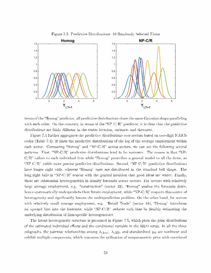
Figure 7.3: Predictive Distributions: 10 Randomly Selected Firms

terms of the Homog predictor, all predictive distributions share the same Gaussian shape paralleling

with each other. On the contrary, in terms of the NP-C/R predictor, it is clear that the predictive

distributions are fairly dierent in the center location, variance, and skewness.

Figure 7.4 further aggregates the predictive distributions over sectors based on two-digit NAICS

codes (Table 7.4). It plots the predictive distributions of the log of the average employment within

each sector. Comparing Homog and NP-C/R across sectors, we can see the following several

patterns. First, NP-C/R predictive distributions tend to be narrower. The reason is that NP-

C/R tailors to each individual rm while Homog prescribes a general model to all the rms, so

NP-C/R yields more precise predictive distributions. Second, NP-C/R predictive distributions

have longer right tails, whereas Homog ones are distributed in the standard bell shape. The

long right tails in NP-C/R concur with the general intuition that good ideas are scarce. Finally,

there are substantial heterogeneities in density forecasts across sectors. For sectors with relatively

large average employment, e.g. construction (sector 23), Homog pushes the forecasts down,

hence systematically underpredicts their future employment, while NP-C/R respects this source of

heterogeneity and signicantly lessens the underprediction problem. On the other hand, for sectors

with relatively small average employment, e.g. Retail Trade (sector 44), Homog introduces

an upward bias into the forecasts, while NP-C/R reduces such bias by exibly estimating the

underlying distribution of rm-specic heterogeneities.

The latent heterogeneity structure is presented in Figure 7.5, which plots the joint distributions

of the estimated individual eects and the conditional variable in the R&D setup. In all the three

subgraphs, the pairwise relationships among λi,level, λi,RD, and standardized yi0 are nonlinear and

exhibit multiple components, which reassures the utilization of nonparametric prior with correlated

53

Figure 7.4: Predictive Distributions: Aggregated by Sectors

Subgraph titles are two-digit NAICS codes. Only sectors with more than 10 rms are shown.

54

Table 7.4: Two-digit NAICS Codes

Code Sector

11 Agriculture, Forestry, Fishing and Hunting21 Mining, Quarrying, and Oil and Gas Extraction22 Utilities23 Construction31-33 Manufacturing42 Wholesale Trade44-45 Retail Trade48-49 Transportation and Warehousing51 Information52 Finance and Insurance53 Real Estate and Rental and Leasing54 Professional, Scientic, and Technical Services56 Administrative and Support and Waste Management and Remediation Services61 Educational Services62 Health Care and Social Assistance71 Arts, Entertainment, and Recreation72 Accommodation and Food Services81 Other Services (except Public Administration)

Figure 7.5: Joint Distributions of λi and Condition Variable

random coecients. Furthermore, λi,level, λi,RD, and standardized yi0 are positively correlated with

each other, which roughly indicates that larger rms respond more positively to R&D activities

within the KFS young rm sample.28

28The model here mainly serves the forecasting purpose, so we need to be careful with any causal interpretation.

55

8 Concluding Remarks

This paper proposes a semiparametric Bayesian predictor which performs well in density forecasts

of individuals in a panel data setup. It considers the underlying distribution of individual eects

and pools the information from the whole cross-section in an ecient and exible way. Monte

Carlo simulations and an empirical application to young rm dynamics show that the keys for the

better density forecasts are, in order of importance, nonparametric Bayesian prior, cross-sectional

heteroskedasticity, and correlated random coecients.

Moving forward, I plan to extend my research in the following several directions:

Theoretically, I will continue the Bayesian asymptotic discussion with strong posterior consis-

tency and rates of convergence.

Methodologically, I will explore some variations of the current setup. First, some empirical

studies may include a large number of covariates with potential heterogeneous eects (i.e. more

variables included in wi,t−1), so it is both theoretically and empirically desirable to investigate

a variable selection scheme in a high-dimensional nonparametric Bayesian framework. Chung and

Dunson (2012) and Liverani et al. (2015) employ variable selection via binary switches, which may be

adaptable to the panel data setting. Another possible direction is to construct a Bayesian-Lasso-type

estimator coherent with the current nonparametric Bayesian implementation. Second, I will consider

panel VAR (Canova and Ciccarelli, 2013), a useful tool to incorporate several variables for each of the

individuals and to jointly model the evolution of these variables, allowing us to take more information

into account for forecasting purposes and oer richer insights into the latent heterogeneity structure.

Meanwhile, it is also interesting to incorporate extra cross-variable restrictions derived from economic

theories and implement the Bayesian GMM method as proposed in Shin (2014). Third, I will

experiment with nonlinear panel data models, such as the Tobit model that helps accommodate

rms' endogenous exit choice. Such extension would be numerically feasible, but requires further

theoretical work. A natural next step would be extending the theoretical discussion to the family of

generalized linear models.

56

References

Akcigit, U. and Kerr, W. R. (2010). Growth through heterogeneous innovations.

Amewou-Atisso, M., Ghosal, S., Ghosh, J. K. and Ramamoorthi, R. V. (2003). Posterior

consistency for semi-parametric regression problems. Bernoulli, 9 (2), 291312.

Amisano, G. and Geweke, J. (2016). Prediction using several macroeconomic models. The Review

of Economics and Statistics, forthcoming.

and Giacomini, R. (2007). Comparing density forecasts via weighted likelihood ratio tests.

Journal of Business & Economic Statistics, 25 (2), 177190.

Antoniak, C. E. (1974). Mixtures of Dirichlet processes with applications to Bayesian nonpara-

metric problems. The Annals of Statistics, pp. 11521174.

Arellano, M. and Bonhomme, S. (2012). Identifying distributional characteristics in random

coecients panel data models. The Review of Economic Studies, 79 (3), 9871020.

and Bover, O. (1995). Another look at the instrumental variable estimation of error-components

models. Journal of Econometrics, 68 (1), 29 51.

Atchadé, Y. F. and Rosenthal, J. S. (2005). On adaptive Markov chain Monte Carlo algorithms.

Bernoulli, 11 (5), 815828.

Basu, S. and Chib, S. (2003). Marginal likelihood and Bayes factors for Dirichlet process mixture

models. Journal of the American Statistical Association, 98 (461), 224235.

Blackwell, D. and Dubins, L. (1962). Merging of opinions with increasing information. The

Annals of Mathematical Statistics, 33 (3), 882886.

Burda, M. and Harding, M. (2013). Panel probit with exible correlated eects: quantifying

technology spillovers in the presence of latent heterogeneity. Journal of Applied Econometrics,

28 (6), 956981.

, and Hausman, J. (2012). A Poisson mixture model of discrete choice. Journal of Economet-

rics, 166 (2), 184203.

Canova, F. and Ciccarelli, M. (2013). Panel Vector Autoregressive Models: A Survey. Working

Paper Series, European Central Bank 1507, European Central Bank.

Chung, Y. and Dunson, D. B. (2012). Nonparametric bayes conditional distribution modeling

with variable selection. Journal of the American Statistical Association.

57

Delaigle, A., Hall, P. andMeister, A. (2008). On deconvolution with repeated measurements.

The Annals of Statistics, pp. 665685.

Diaconis, P. and Freedman, D. (1986). On inconsistent Bayes estimates of location. The Annals

of Statistics, pp. 6887.

Diebold, F. X., Gunther, T. A. and Tay, A. S. (1998). Evaluating density forecasts with

applications to nancial risk management. International Economic Review, 39 (4), 863883.

and Mariano, R. S. (1995). Comparing predictive accuracy. Journal of Business & Economic

Statistics, 13 (3).

Doob, J. L. (1949). Application of the theory of martingales. Le calcul des probabilites et ses

applications, pp. 2327.

Dunson, D. B. (2009). Nonparametric Bayes local partition models for random eects. Biometrika,

96 (2), 249262.

and Park, J.-H. (2008). Kernel stick-breaking processes. Biometrika, 95 (2), 307323.

Efron, B. (2012). Large-scale Inference: Empirical Bayes Methods for Estimation, Testing, and

Prediction, vol. 1. Cambridge University Press.

Escobar, M. D. andWest, M. (1995). Bayesian density estimation and inference using mixtures.

Journal of the American Statistical Association, 90 (430), 577588.

Fernandez, C. and Steel, M. F. (2000). Bayesian regression analysis with scale mixtures of

normals. Econometric Theory, 16 (01), 80101.

Freedman, D. A. (1963). On the asymptotic behavior of Bayes' estimates in the discrete case. The

Annals of Mathematical Statistics, pp. 13861403.

(1965). On the asymptotic behavior of Bayes estimates in the discrete case II. The Annals of

Mathematical Statistics, 36 (2), 454456.

Galambos, J. and Simonelli, I. (2004). Products of Random Variables: Applications to Problems

of Physics and to Arithmetical Functions. Marcel Dekker.

Geweke, J. and Amisano, G. (2010). Comparing and evaluating Bayesian predictive distributions

of asset returns. International Journal of Forecasting, 26 (2), 216230.

Ghosal, S., Ghosh, J. K., Ramamoorthi, R. et al. (1999). Posterior consistency of Dirichlet

mixtures in density estimation. The Annals of Statistics, 27 (1), 143158.

Ghosh, J. K. and Ramamoorthi, R. (2003). Bayesian Nonparametrics. Springer-Verlag.

58

Griffin, J. E. (2016). An adaptive truncation method for inference in Bayesian nonparametric

models. Statistics and Computing, 26 (1), 423441.

Gu, J. and Koenker, R. (2015). Unobserved heterogeneity in income dynamics: an empirical

Bayes perspective. Journal of Business & Economic Statistics, forthcoming.

and (2016). Empirical Bayesball remixed: empirical Bayes methods for longitudinal data.

Journal of Applied Econometrics, pp. n/an/a.

Hall, B. H. and Rosenberg, N. (2010). Handbook of the Economics of Innovation, vol. 1. Elsevier.

Haltiwanger, J., Jarmin, R. S. and Miranda, J. (2012). Who creates jobs? Small versus large

versus young. Review of Economics and Statistics, 95 (2), 347361.

Hastie, D. I., Liverani, S. and Richardson, S. (2015). Sampling from Dirichlet process mixture

models with unknown concentration parameter: mixing issues in large data implementations.

Statistics and Computing, 25 (5), 10231037.

Hirano, K. (2002). Semiparametric Bayesian inference in autoregressive panel data models. Econo-

metrica, 70 (2), 781799.

Hjort, N. L., Holmes, C., Müller, P. and Walker, S. G. (2010). Bayesian Nonparametrics.

Cambridge University Press.

Ishwaran, H. and James, L. F. (2001). Gibbs sampling methods for stick-breaking priors. Journal

of the American Statistical Association, 96 (453), 161173.

and (2002). Approximate Dirichlet process computing in nite normal mixtures: smoothing

and prior information. Journal of Computational and Graphical Statistics, 11 (3), 508532.

James, W. and Stein, C. (1961). Estimation with quadratic loss. In Proceedings of the Fourth

Berkeley Symposium on Mathematical Statistics and Probability, Volume 1: Contributions to the

Theory of Statistics, Berkeley, Calif.: University of California Press, pp. 361379.

Jensen, M. J., Fisher, M. and Tkac, P. (2015). Mutual fund performance when learning the

distribution of stock-picking skill.

Kalli, M., Griffin, J. E. and Walker, S. G. (2011). Slice sampling mixture models. Statistics

and Computing, 21 (1), 93105.

Kelker, D. (1970). Distribution theory of spherical distributions and a location-scale parameter

generalization. Sankhya: The Indian Journal of Statistics, Series A, pp. 419430.

Lee, Y., Amaral, L. A. N., Canning, D., Meyer, M. and Stanley, H. E. (1998). Universal

features in the growth dynamics of complex organizations. Physical Review Letters, 81 (15), 3275.

59

Liu, L.,Moon, H. R. and Schorfheide, F. (2016). Forecasting with dynamic panel data models.

Liverani, S., Hastie, D. I., Azizi, L., Papathomas, M. andRichardson, S. (2015). PReMiuM:

an R package for prole regression mixture models using Dirichlet processes. Journal of Statistical

Software, 64 (7).

Marcellino, M., Stock, J. H. and Watson, M. W. (2006). A comparison of direct and iter-

ated multistep AR methods for forecasting macroeconomic time series. Journal of Econometrics,

135 (1), 499526.

Neal, R. M. (2000). Markov chain sampling methods for Dirichlet process mixture models. Journal

of Computational and Graphical Statistics, 9 (2), 249265.

Norets, A. (2010). Approximation of conditional densities by smooth mixtures of regressions. The

Annals of Statistics, 38 (3), 17331766.

and Pelenis, J. (2012). Bayesian modeling of joint and conditional distributions. Journal of

Econometrics, 168 (2), 332346.

and (2014). Posterior consistency in conditional density estimation by covariate dependent

mixtures. Econometric Theory, 30, 606646.

Papaspiliopoulos, O. and Roberts, G. O. (2008). Retrospective Markov chain Monte Carlo

methods for Dirichlet process hierarchical models. Biometrika, 95 (1), 169186.

Pati, D., Dunson, D. B. and Tokdar, S. T. (2013). Posterior consistency in conditional distri-

bution estimation. Journal of Multivariate Analysis, 116, 456472.

Pav, S. E. (2015). Moments of the log non-central chi-square distribution. arXiv preprint

arXiv:1503.06266.

Pelenis, J. (2014). Bayesian regression with heteroscedastic error density and parametric mean

function. Journal of Econometrics, 178, 624638.

Robb, A., Ballou, J., DesRoches, D., Potter, F., Zhao, Z. and Reedy, E. (2009). An

overview of the Kauman Firm Survey: results from the 2004-2007 data. Available at SSRN

1392292.

and Seamans, R. (2014). The role of R&D in entrepreneurial nance and performance. Available

at SSRN 2341631.

Robbins, H. (1956). An empirical Bayes approach to statistics. In Proceedings of the Third Berkeley

Symposium on Mathematical Statistics and Probability, University of California Press, Berkeley

and Los Angeles.

60

Rossi, P. E. (2014). Bayesian Non- and Semi-parametric Methods and Applications. Princeton

University Press.

Santarelli, E., Klomp, L. and Thurik, A. R. (2006). Gibrat's law: an overview of the empirical

literature. In Entrepreneurship, Growth, and Innovation, Springer, pp. 4173.

Schwartz, L. (1965). On Bayes procedures. Zeitschrift für Wahrscheinlichkeitstheorie und ver-

wandte Gebiete, 4 (1), 1026.

Sethuraman, J. (1994). A constructive denition of Dirichlet priors. Statistica Sinica, pp. 639650.

Shin, M. (2014). Bayesian GMM.

Tokdar, S. T. (2006). Posterior consistency of Dirichlet location-scale mixture of normals in density

estimation and regression. Sankhya: The Indian Journal of Statistics, pp. 90110.

Walker, S. G. (2007). Sampling the Dirichlet mixture model with slices. Communications in

Statistics - Simulation and Computation, 36 (1), 4554.

Wu, Y. and Ghosal, S. (2008). Kullback Leibler property of kernel mixture priors in Bayesian

density estimation. Electronic Journal of Statistics, 2, 298331.

Yau, C., Papaspiliopoulos, O., Roberts, G. O. and Holmes, C. (2011). Bayesian non-

parametric hidden Markov models with applications in genomics. Journal of the Royal Statistical

Society: Series B (Statistical Methodology), 73 (1), 3757.

Zarutskie, R. andYang, T. (2015). How did young rms fare during the great recession? Evidence

from the Kauman Firm Survey. In Measuring Entrepreneurial Businesses: Current Knowledge

and Challenges, University of Chicago Press.

61

A Notations

U (a, b) represents a uniform distribution with minimum value a and maximum value b. If a = 0

and b = 1, we obtain the standard uniform distribution, U (0, 1).

N(µ, σ2

)or N

(x;µ, σ2

)stands for a Gaussian distribution with mean µ and variance σ2.

Its probability distribution function (pdf) is given by φ(x;µ, σ2

). When µ = 0 and σ2 = 1 (i.e.

standard normal), we reduce the notation to φ (x). The corresponding cumulative distribution

functions (cdf) are denoted as Φ(x;µ, σ2

)and Φ (x), respectively. The same convention holds for

multivariate normal, where N (µ,Σ), N (x;µ,Σ), φ (x;µ,Σ), and Φ (x;µ,Σ) are for the distribution

with the mean vector µ and the covariance matrix Σ.

TN(µ, σ2, a, b

)denotes a truncated normal distribution with µ and σ2 being the mean and

variance before truncation, and a and b being the lower and upper end of the truncated interval.

The gamma distribution is denoted as Ga (x; a, b) with pdf being fGa (x; a, b) = ba

Γ(a)xa−1e−bx.

The according inverse-gamma distribution is given by IG (x; a, b) with pdf being fIG (x; a, b) =ba

Γ(a)x−a−1e−b/x. The Γ (·) in the denominators is the gamma function.

The inverse Wishart distribution is a generalization of the inverse gamma distribution to

multi-dimensional setups. Let Ω be a d× d matrix, then the inverse Wishart distribution is denoted

as IW (Ω; Ψ, ν), and its pdf is fIW (Ω; Ψ, ν) = |Ψ|ν2

2νd2 Γd( ν

2)|Ω|−

ν+d+12 e−

12tr(ΨΩ−1). When Ω is a scalar,

the inverse Wishart distribution is reduced to a inverse-gamma distribution with a = ν/2, b = Ψ/2.

1 (·) is an indicator function that equals 1 if the condition in the parenthesis is satised and

equals 0 otherwise.

IN is an N ×N identity matrix.

In the panel data setup, for a generic variable z, which can be v, w , x, or y, zit is a dz × 1

vector, and zi,t1:t2 = (zit1 , · · · , zit2) is a dz × (t2 − t1 + 1) matrix.

‖·‖ represents the Euclidean norm, i.e. for a n-dimensional vector z = [z1, z2, · · · , zn]′,

‖z‖ =√z2

1 + · · ·+ z2n.

supp (·) denotes the support of a probability measure.

B Algorithms

B.1 Hyperparameters

Recall the prior for the common parameters:

(β, σ2

)∼ N

(mβ

0 , ψβ0σ

2)IG(σ2; aσ

2

0 , bσ2

0

).

A-1

The hyperparameters are chosen in a relatively ignorant sense without inferring too much from the

data except aligning the scale according to the variance of the data.

aσ2

0 = 2, (B.1)

bσ2

0 = Ei(V ar

t

i (yit))·(aσ

2

0 − 1)

= Ei(V ar

t

i (yit)), (B.2)

mβ0 = 0.5, (B.3)

ψβ0 =1

bσ2

0 /(aσ

2

0 − 1) =

1

Ei(V ar

t

i (yit)) . (B.4)

In equation (B.2) here and equation (B.5) below, Eti and V art

i stand for the sample mean and

variance for rm i over t = 1, · · · , T , and Ei and V ariare the sample mean and variance over the

whole cross-section i = 1, · · · , N . Equation (B.2) ensures that on average the prior and the data have

a similar scale. Equation (B.3) conjectures that the young rm dynamics are highly likely persistent

and stationary. Since we don't have strong prior information in the common parameters, their priors

are chosen to be not very restrictive. Equation (B.1) characterizes a rather less informative prior on

σ2 with innite variance, and Equation (B.4) assumes that the prior variance of β is equal to 1 on

average.

The hyperpriors for the DPM prior are specied as:

G0

(µk, ω

2k

)= N

(µk; m

λ0 , ψ

λ0ω

2k

)IG(ω2k; a

λ0 , b

λ0

),

α ∼ Ga (α; aα0 , bα0 ) .

Similarly, the hyperparameters are chosen to be:

aλ0 = 2, bλ0 = V ari(Eti (yit)

)·(aλ0 − 1

)= V ar

i(Eti (yit)

), (B.5)

mλ0 = 0, ψλ0 = 1,

aα0 = 2, bα0 = 2. (B.6)

where bλ0 is selected to match the scale, while aλ0 , mλ0 , and ψ

λ0 yields a relatively ignorant and diuse

prior. Following Ishwaran and James (2001, 2002), the hyperparameters for the DP scale parameter

α in equation (B.6) allows for a exible component structure with a wide range of component

numbers. The truncated number of components is set to be K = 50, so that the approximation

error is uniformly bounded by Ishwaran and James (2001) Theorem 2:∥∥∥fλ,K − fλ∥∥∥ ∼ 4N exp

(−K − 1

α

)≤ 2.10× 10−18,

at the prior mean of α (α = 1) and cross-sectional sample size N = 1000.

A-2

I have also examined other choices of hyperparameters, and results are not very sensitive to

hyperparameters as long as the implied priors are exible enough to cover the range of observables.

B.2 Random-Walk Metropolis-Hastings

When there is no closed-form conditional posterior distribution in some MCMC steps, it is help-

ful to employ the Metropolis-within-Gibbs sampler and use the random-walk Metropolis-Hastings

(RWMH) algorithm for those steps. The adaptive RWMH algorithm below is based on Atchadé and

Rosenthal (2005) and Grin (2016), which adaptively adjust the random walk step size in order to

keep acceptance rates around certain desirable percentage.

Algorithm B.1. (Adaptive RWMH)

Let us consider a generic variable θ. For each iteration s = 1, · · · , nsim,1. Draw candidate θ from the random-walk proposal density θ ∼ N

(θ(s−1), ζ(s)Σ

).

2. Calculate the acceptance rate

a.r.(θ|θ(s−1)) = min

(1,

p(θ|·)p(θ(s−1)|·)

),

where p(θ|·) is the conditional posterior distribution of interest.

3. Accept the proposal and set θ(s) = θ with probability a.r.(θ|θ(s−1)). Otherwise, reject the

proposal and set θ(s) = θ(s−1).

4. Update the random-walk step size for the next iteration,

log ζ(s+1) = ρ(

log ζ(s) + s−c(a.r.(θ|θ(s−1))− a.r.?

)),

where 0.5 < c ≤ 1, a.r.? is the target acceptance rate, and

ρ (x) = min (|x|, x) · sgn (x) ,

where x > 0 is a very large number.

Remark B.2. (i) In step 1, since the algorithms in this paper only consider RWMH on conditionally

independent scalar variables, Σ is simply taken to be 1.

(ii) In step 4, I choose c = 0.55, a.r.? = 30% in the numerical exercises, following Grin (2016).

B.3 Details on Posterior Samplers

The formulas below focus on the (correlated) random coecients model in Algorithms 5.1 and 5.2

where the (correlated) random eects model in Algorithms 3.1 and 3.2 are special cases with solely

univariate λi.

A-3

B.3.1 Step 2: Component Parameters

Random Coecients Model For z = λ, l and kz = 1, · · · ,Kz, draw(µz(s)kz ,Ω

z(s)kz

)from a

multivariate-normal-inverse-Wishart distribution (or a normal-inverse-gamma distribution if z is a

scalar) p

(µz(s)kz ,Ω

z(s)kz

∣∣∣∣z(s−1)i

i∈Jz(s−1)

kz

):

(µz(s)kz ,Ω

z(s)kz

)∼ N

(µz(s)kz ; mz

kz , ψzkzΩ

z(s)kz

)IW(

Ωz(s)kz ; Ψz

kz , νzkz

),

mzkz =

1

nz(s−1)kz

∑i∈Jz(s−1)

kz

z(s−1)i ,

ψzkz =(

(ψz0)−1 + nz(s−1)kz

)−1,

mzkz = ψzkz

(ψz0)−1mz0 +

∑i∈Jz(s−1)

kz

z(s−1)i

,

νzkz = νz0 + nz(s−1)kz ,

Ψzkz = Ψz

0 +∑

i∈Jz(s−1)kz

(z

(s−1)i

)2+mz′

0 (ψz0)−1mz0 −mz′

kz (ψzkz)−1mz

kz .

Correlated Random Coecients Model Due to the complexity arising from the conditional

structure, I break the updating procedure for(µz(s)kz ,Ω

z(s)kz

)into two steps. For z = λ, l and

kz = 1, · · · ,Kz,

(a) Draw µz(s)kz from a matricvariate-normal distribution (or a multivariate-normal distribution

if z is a scalar) p

(µz(s)kz

∣∣∣∣Ωz(s−1)kz ,

z

(s−1)i , ci0

i∈Jz(s−1)

kz

):

vec(µz(s)kz

)∼ N

(vec(µz(s)kz

); vec (mz

kz) , ψzkz

),

mz,zckz =

∑i∈Jz(s−1)

kz

z(s−1)i

[1, c′i0

],

mz,cckz =

∑i∈Jz(s−1)

kz

[1, c′i0

]′ [1, c′i0

],

mzkz = mz,zc

kz

(mz,cckz

)−1,

ψzkz =

[(ψz0)−1 + mz,cc

kz ⊗(

Ωz(s−1)kz

)−1]−1

,

vec (mzkz) = ψzkz

[(ψz0)−1 vec (mz

0) +

(mz,cckz ⊗

(Ωz(s−1)kz

)−1)vec (mz

kz)

],

where vec (·) denotes matrix vectorization, and ⊗ is the Kronecker product.

(b) Draw Ωz(s)kz from an inverse-Wishart distribution (or an inverse-gamma distribution if z is a

A-4

scalar) p

(Ωz(s)kz

∣∣∣∣µz(s)kz ,z

(s−1)i , ci0

i∈Jz(s−1)

kz

):

Ωz(s)kz ∼ IW

(Ωz(s)kz ; Ψz

kz , νzkz

),

νzkz = νz0 + nz(s−1)kz ,

Ψzkz = Ψz

0 +∑

i∈Jz(s−1)kz

(z

(s−1)i − µz(s)kz

[1, c′i0

]′)(z

(s−1)i − µz(s)kz

[1, c′i0

]′)′.

B.3.2 Step 4: Individual-specic Parameters

For i = 1, · · · , N , draw λ(s)i from a multivariate-normal distribution (or a normal distribution if λ

is a scalar) p(λ

(s)i

∣∣∣µλ(s)

γλi,Ω

λ(s)

γλi,(σ2i

)(s−1), β(s−1), Di, DA

):

λ(s)i ∼ N

(mλi ,Σ

λi

),

Σλi =

((Ωλ(s)

γλi

)−1+((σ2i

)(s−1))−1

t1i∑t=t0i

wi,t−1w′i,t−1

)−1

,

mλi = Σλ

i

((Ωλ(s)

γλi

)−1µλi +

((σ2i

)(s−1))−1

t1i∑t=t0i

wi,t−1

(yit − β(s−1)′xi,t−1

)),

where the conditional prior mean is characterized by

µλi =

µλ(s)

γλi, for the random coecients model,

µλ(s)

γλi[1, c′i0]′ , for the correlated random coecients model.

A-5

B.3.3 Step 5: Common parameters

Cross-sectional Homoskedasticity Draw(β(s), σ2(s)

)from a linear regression model with un-

known variance, p(β(s), σ2(s)

∣∣∣λ(s)i

, D

):

(β(s), σ2(s)

)∼ N

(β(s); mβ, ψβσ2(s)

)IG(σ2(s); aσ

2, bσ

2),

ψβ =

((ψβ0

)−1+

N∑i=1

t1i∑t=t0i

xi,t−1x′i,t−1

)−1

,

mβ = ψβ

((ψβ0

)−1mβ

0 +N∑i=1

t1i∑t=t0i

xi,t−1

(yit − λ(s)′

i wi,t−1

)),

aσ2

= aσ2

0 +NT

2

bσ2

= bσ2

0 +1

2

(N∑i=1

T∑t=1

(yit − λ(s)′

i wi,t−1

)2+mβ′

0

(ψβ0

)−1mβ

0 −mβ′(ψβ)−1

mβ

).

Cross-sectional Heteroskedasticity Draw β(s) from a linear regression model with known

variance, p(β(s)

∣∣∣λ(s)i ,(σ2i

)(s), D

):

β(s) ∼ N(mβ,Σβ

),

Σβ =

((Σβ

0

)−1+((σ2i

)(s))−1N∑i=1

t1i∑t=t0i

xi,t−1x′i,t−1

)−1

,

mβ = Σβ

((Σβ

0

)−1mβ

0 +((σ2i

)(s))−1N∑i=1

t1i∑t=t0i

xi,t−1

(yit − λ(s)′

i wi,t−1

)).

Remark B.3. For unbalanced panels, the summations and products in steps 4 and 5 (Subsections

B.3.2 and B.3.3) are instead over t = t0i, · · · , t1i, the observed periods for individual i.

B.4 Slice-Retrospective Samplers

The next algorithm borrows the idea from some recent development in DPM sampling strategies

(Dunson, 2009; Yau et al., 2011; Hastie et al., 2015), which integrates the slice sampler (Walker,

2007; Kalli et al., 2011) and the retrospective sampler (Papaspiliopoulos and Roberts, 2008). By

adding extra auxiliary variables, the sampler is able to avoid hard truncation in Ishwaran and James

(2001, 2002). I experiment with it to check whether the approximation error due to truncation would

signicantly aect the density forecasts or not, and the results do not change much. The following

algorithm is designed for the random coecient case. A corresponding version for the correlated

random coecient case can be constructed in a similar manner.

A-6

The auxiliary variables uzi , i = 1, · · · , N , are i.i.d. standard uniform random variables, i.e.

uzi ∼ U (0, 1). Then, the mixture of components in equation (2.6) can be rewritten as

z ∼∞∑

kz=1

1 (uzi < pzikz) fz (z; θzkz) ,

where z = λ, l. By marginalizing over uzi , we can recover equation (2.6). Accordingly, we can dene

the number of active components as

Kz,A = max1≤i≤N

γzi ,

and the number of potential components (including active components) as

Kz,P = min

kz :

1−kz∑j=1

pzj

< min1≤i≤N

uzi

.

Although the number of components is innite literally, we only need to care about the components

that can potentially be occupied. Therefore, Kz,P serves as an upper limit on the number of

components that need to be updated at certain iteration. Here I suppress the iteration indicator

s for exposition simplicity, but note that both Kz,A and Kz,P can change over iterations; this is

indeed the highlight of this sampler.

Algorithm B.4. (General Model: Random Coecients III (Slice-Retrospective))

For each iteration s = 1, · · · , nsim, steps 1-3 in Algorithm 5.1 are modied as follows:

For z = λ, l,

1. Active components:

(a) Number of active components:

Kz,A = max1≤i≤N

γz(s−1)i .

(b) Component probabilities: for kz = 1, · · · ,Kz,A, draw pz∗kz from the stick breaking process

p(pz∗kz

∣∣∣αz(s−1),nz(s−1)kz

):

pz∗kz ∼ SB

nz(s−1)kz , αz(s−1) +

Kz,A∑j=kz+1

nz(s−1)j

, kz = 1, · · · ,Kz,A.

(c) Component parameters: for kz = 1, · · · ,Kz,A, draw θz∗kz from p

(θz∗kz

∣∣∣∣z(s−1)i

i∈Jz(s−1)

kz

)as in Algorithm 3.1 step 2.

(d) Label switching: jointly updatepz(s)kz , θ

z(s)kz , γz∗i

Kz,A

kz=1based on

pz∗kz , θ

z∗kz , γ

z(s−1)i

Kz,A

kz=1by

three Metropolis-Hastings label-switching moves:

A-7

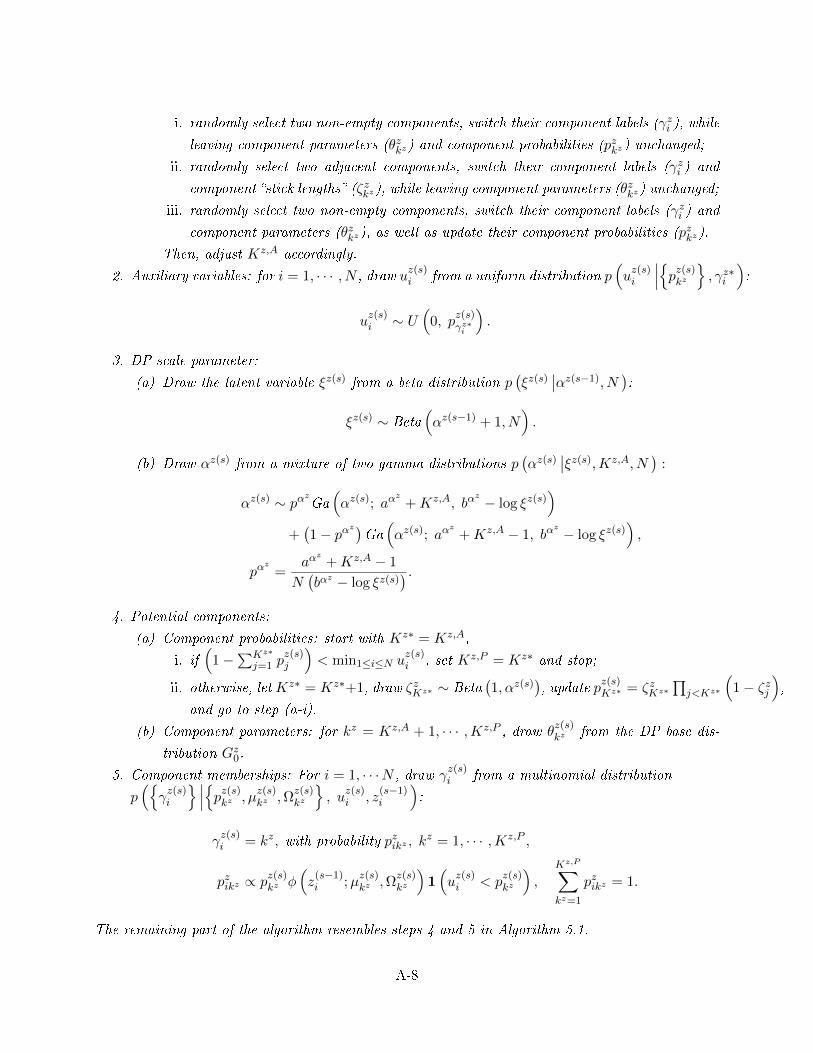
i. randomly select two non-empty components, switch their component labels (γzi ), while

leaving component parameters (θzkz) and component probabilities (pzkz) unchanged;

ii. randomly select two adjacent components, switch their component labels (γzi ) and

component stick lengths (ζzkz), while leaving component parameters (θzkz) unchanged;

iii. randomly select two non-empty components, switch their component labels (γzi ) and

component parameters (θzkz), as well as update their component probabilities (pzkz).

Then, adjust Kz,A accordingly.

2. Auxiliary variables: for i = 1, · · · , N , draw uz(s)i from a uniform distribution p

(uz(s)i

∣∣∣pz(s)kz

, γz∗i

):

uz(s)i ∼ U

(0, p

z(s)γz∗i

).

3. DP scale parameter:

(a) Draw the latent variable ξz(s) from a beta distribution p(ξz(s)

∣∣αz(s−1), N):

ξz(s) ∼ Beta(αz(s−1) + 1, N

).

(b) Draw αz(s) from a mixture of two gamma distributions p(αz(s)

∣∣ξz(s),Kz,A, N)

:

αz(s) ∼ pαzGa(αz(s); aα

z+Kz,A, bα

z − log ξz(s))

+(1− pαz

)Ga(αz(s); aα

z+Kz,A − 1, bα

z − log ξz(s)),

pαz

=aα

z+Kz,A − 1

N(bαz − log ξz(s)

) .4. Potential components:

(a) Component probabilities: start with Kz∗ = Kz,A,

i. if(

1−∑Kz∗

j=1 pz(s)j

)< min1≤i≤N u

z(s)i , set Kz,P = Kz∗ and stop;

ii. otherwise, letKz∗ = Kz∗+1, draw ζzKz∗ ∼ Beta(1, αz(s)

), update p

z(s)Kz∗ = ζzKz∗

∏j<Kz∗

(1− ζzj

),

and go to step (a-i).

(b) Component parameters: for kz = Kz,A + 1, · · · ,Kz,P , draw θz(s)kz from the DP base dis-

tribution Gz0.

5. Component memberships: For i = 1, · · ·N , draw γz(s)i from a multinomial distribution

p(γz(s)i

∣∣∣pz(s)kz , µz(s)kz ,Ω

z(s)kz

, u

z(s)i , z

(s−1)i

):

γz(s)i = kz, with probability pzikz , k

z = 1, · · · ,Kz,P ,

pzikz ∝ pz(s)kz φ

(z

(s−1)i ;µ

z(s)kz ,Ω

z(s)kz

)1(uz(s)i < p

z(s)kz

),

Kz,P∑kz=1

pzikz = 1.

The remaining part of the algorithm resembles steps 4 and 5 in Algorithm 5.1.

A-8

Remark B.5. Note that:

(i) Steps 1-b,c,d are sampling from marginal posterior of (pzkz , θzkz , γ

zi ) for the active components

with the auxiliary variables uzi s being integrated out. Thus, extra caution is needed in dealing with

the order of the steps.

(ii) The label switching moves 1-d-i and 1-d-ii are based on Papaspiliopoulos and Roberts (2008),

and 1-d-iii is suggested by Hastie et al. (2015). All these label switching moves aim to improve

numerical convergence.

(iii) Step 3 for DP scale parameter αz follows Escobar and West (1995). It is dierent from step

1-a in Algorithm 5.1 due to the unrestricted number of components in the current sampler.

(iv) Steps 4-a-ii and 4-b that update potential components are very similar to steps 1-b and 1-c

that update active componentsjust take Jzkz as an empty set and draw directly from the prior.

(v) The auxiliary variable uzi also appears in step 5 that updates component memberships. The

inclusion of auxiliary variables helps determine a nite set of relevant components for each individual

i without mechanically truncating the innite mixture.

C Proofs for Baseline Model

C.1 Posterior Consistency: Random Eects Model

C.1.1 Skills vs Shocks

Proof. (Proposition 4.7)

Based on the Schwartz (1965) theorem stated in Lemma 4.6, two sucient conditions guarantee

the posterior consistency: KL requirement and uniformly exponentially consistent tests.

(i) KL requirement

The proposition assumes that the KL property holds for the distribution of λ, i.e. for all ε > 0,

Πf

(f ∈ F :

ˆf0 (λ) log

f0 (λ)

f (λ)dλ < ε

)> 0,

whose sucient conditions are stated in Lemmas 4.8 and E.1. On the other hand, the KL requirement

is specied on the observed y in order to guarantee that the denominator in equation (4.2) is large

enough. In this sense, we need to establish that for all ε > 0,

Π

(f ∈ F :

ˆf0 (y − u)φ (u) log

´f0 (y − u′)φ (u′) du′´f (y − u′)φ (u′) du′

dudy < ε

)> 0.

Let g (x) = x log x, a (u) = f0 (y − u)φ (u), A =´a (u) du, b (u) = f (y − u)φ (u), B =

´b (u) du.

A-9

We can rewrite the integral over u as

ˆf0 (y − u)φ (u) log

´f0 (y − u′)φ (u′) du′´f (y − u′)φ (u′) du′

du = A · logA

B= B · g

(A

B

)=B · g

(ˆb (u)

B· f0 (y − u)

f (y − u)du

)≤ˆb (u) g

(f0 (y − u)

f (y − u)

)du

=

ˆφ (u) f0 (y − u) log

f0 (y − u)

f (y − u)du, (C.1)

where the inequality is given by Jensen's inequality. Then, further integrating the above expression

over y, we have

ˆf0 (y − u)φ (u) log

´f0 (y − u′)φ (u′) du′´f (y − u′)φ (u′) du′

dudy ≤ˆφ (u) f0 (y − u) log

f0 (y − u)

f (y − u)dudy

=

ˆφ (u) du ·

ˆf0 (λ) log

f0 (λ)

f (λ)dλ = ε

The inequality follows the above expression (C.1), the next equality is given by change of variables,

and the last equality is given by the KL property of the distribution of λ.

(ii) Uniformly exponentially consistent tests

(ii-a) When λ is observed

Note that by the Hoeding's inequality, the uniformly exponentially consistent tests are equiva-

lent to strictly unbiased tests, so we only need to construct a test function ϕ? such that

Ef0 (ϕ?) < inff∈Uc

Ef (ϕ?) .

Without loss of generality, let us consider a weak neighborhood dened on ε > 0 and a bounded

continuous function ϕ ranging from 0 to 1. Then, the corresponding neighborhood is given by

Uε,ϕ (f0) =

f :

∣∣∣∣ˆ ϕf −ˆϕf0

∣∣∣∣ < ε

.

We can divide the alternative region into two parts29

U cε,ϕ (f0) = A1 ∪A2

29It is legitimate to divide the alternatives into sub-regions. Intuitively, with dierent alternative sub-regions, thenumerator in equation (4.2) is composed of integrals over dierent domains, and all of them converge to 0.

A-10

where

A1 =

f :

ˆϕf >

ˆϕf0 + ε

,

A2 =

f :

ˆϕf <

ˆϕf0 − ε

.

For A1, we can choose the test function ϕ? to be ϕ. For A2, we can choose ϕ? to be 1 − ϕ. Then,in either case A = A1, A2, type I error Ef0 (ϕ?) =

´ϕ?f0, and power inff∈A Ef (ϕ?) ≥

´ϕ?f0 + ε,

hence the tests exist when λ is observed.

(ii-b) When y is observed instead of λ

Dene g (λ) = f (λ)− f0 (λ). Then, by denition,´g (λ) dλ = 0 for all g. There are always tests

if we observe λ, then for any g, there exists a ε > 0 such that

ˆ|g (λ)| dλ > ε. (C.2)

The next step is to prove that there are tests when y is observed instead of λ, which is done via

proof by contradiction. Suppose there is no test when we only observe y, then there exists a g such

that

h (y) =

ˆg (y − u)φ (u) du = 0 for all y,

due to the continuity of h. Employing the Fourier transform, we have

Fy (ξ) = Fλ (ξ) · c1 exp(−c2ξ

2)

= 0 for all ξ.

Since c1 exp(−c2ξ

2)6= 0, then

Fλ (ξ) = 0 for all ξ.

Finally, the inverse Fourier transform leads to

g (λ) = 0 for all λ,

which contradicts equation (C.2). Therefore, there are also tests when y is observed instead of λ.

Combining (i) and (ii-b), f achieves posterior consistency even when we only observe y.

C.1.2 Unknown Shocks Sizes

Proof. (Proposition 4.9)

(i) KL requirement

Based on the observed sucient statistics λ = 1T

∑Tt=1 yit with corresponding errors u = 1

T

∑Tt=1 uit,

A-11

the KL requirement can be written as follows: for all ε > 0,

Π

f ∈ F , σ2 ∈ R+ :

ˆf0

(λ− u

)φ

(u; 0,

σ20

T

)log

´f0

(λ− u′

)φ(u′; 0,

σ20T

)du′

´f(λ− u′

)φ(u′; 0, σ

2

T

)du′

dudλ < ε

> 0.

Under the prior specication together with hyperparameters specied in Appendix B.1, the integral

is bounded with probability one. Following the dominated convergence theorem,

limσ2→σ2

0

ˆf0

(λ− u

)φ

(u; 0,

σ20

T

)log

´f0

(λ− u′

)φ(u′; 0,

σ20T

)du′

´f(λ− u′

)φ(u′; 0, σ

2

T

)du′

dudλ

=

ˆf0

(λ− u

)φ

(u; 0,

σ20

T

)log

´f0

(λ− u′

)φ(u′; 0,

σ20T

)du′

´f(λ− u′

)φ(u′; 0,

σ20T

)du′

dudλ,

where the upper bound of the right hand side can be characterized by the KL property of the

distribution of λ as in the proof of Proposition 4.7 part (i). The sucient conditions of the KL

property of the distribution of λ are stated in Lemmas 4.8 and E.1.

(ii) Uniformly exponentially consistent tests

The alternative region can be split into the following two parts:

(ii-a)∣∣σ2 − σ2

0

∣∣ > ∆

Orthogonal forward dierencing yields yit ∼ N(0, σ2

0

). Then, as N →∞,

1N(T−1)

∑Ni=1

∑T−1t=1 (yit)

2

σ20

∼ χ2N(T−1)

d→ N

(1,

2

N (T − 1)

).

Note that for a generic variable x ∼ N (0, 1), for x∗ > 0,

P (x > x∗) ≤ φ (x∗)

x∗. (C.3)

Then, we can directly construct the following test function

ϕN (y1:N,1:T−1) =

1

(1

N(T−1)

∑Ni=1

∑T−1t=1 (yit)

2

σ20

< 1− ∆2σ2

0

), for σ2 < σ2

0 −∆,

1

(1

N(T−1)

∑Ni=1

∑T−1t=1 (yit)

2

σ20

> 1 + ∆2σ2

0

), for σ2 > σ2

0 + ∆,

which satises the requirements (4.1) for the uniformly exponentially consistent tests.

(ii-b)∣∣σ2 − σ2

0

∣∣ < ∆, f ∈ U cε,Φ (f0)

Without loss of generality, let Φ = ϕ be a singleton and ϕ? be the test function that distin-

A-12

guishes f = f0 versus f ∈ U cε,ϕ (f0) when σ20 is known. Then, we can express the dierence between

Ef (ϕ?) and Ef0 (ϕ?) as

ˆϕ?(λ)f(λ− u

)φ

(u; 0,

σ2

T

)dudλ−

ˆϕ?(λ)f0

(λ− u

)φ

(u; 0,

σ20

T

)dudλ

>

ˆϕ?(λ)(

f(λ− u

)− f0

(λ− u

))φ

(u; 0,

σ20

T

)dudλ

−∣∣∣∣ˆ ϕ?

(λ)f(λ− u

)(φ

(u; 0,

σ2

T

)− φ

(u; 0,

σ20

T

))dudλ

∣∣∣∣ . (C.4)

Since ϕ? is the test function when σ20 is known, the rst term

ˆϕ?(λ)(

f(λ− u

)− f0

(λ− u

))φ

(u; 0,

σ20

T

)dudλ > ε. (C.5)

For the second term,∣∣∣∣ˆ ϕ?(λ)f(λ− u

)(φ

(u; 0,

σ2

T

)− φ

(u; 0,

σ20

T

))dudλ

∣∣∣∣≤ˆϕ?(λ)f(λ− u

) ∣∣∣∣φ(u; 0,σ2

T

)− φ

(u; 0,

σ20

T

)∣∣∣∣ dudλ≤ˆ ∣∣∣∣φ(u; 0,

σ2

T

)− φ

(u; 0,

σ20

T

)∣∣∣∣ du≤√σ2

0

σ2− 1− ln

σ20

σ2. (C.6)

The second inequality is given by the fact that ϕ?(λ)∈ [0, 1]. The last inequality follows Pinsker's

inequality that bounds the total variation distance by the KL divergence, which has an explicit form

for normal distributions

dKL

(φ

(u; 0,

σ20

T

), φ

(u; 0,

σ2

T

))=

1

2

(σ2

0

σ2− 1− ln

σ20

σ2

).

We can choose ∆ > 0 such that for any∣∣σ2 − σ2

0

∣∣ < ∆,√σ2

0

σ2− 1− ln

σ20

σ2<ε

2.

Plugging expressions (C.5) and (C.6) into (C.4), we obtain

ˆϕ?(λ)f(λ− u

)φ

(u; 0,

σ2

T

)dudλ−

ˆϕ?(λ)f0

(λ− u

)φ

(u; 0,

σ20

T

)dudλ > ε− ε

2=ε

2,

so ϕ? is the test function with respect to the alternative sub-region∣∣σ2 − σ2

0

∣∣ < ∆, f ∈ U cε,Φ (f0).

A-13

C.1.3 Lagged Dependent Variables

Proof. (Proposition 4.11)

(i) KL requirement

Dene the sucient statistics λ (β) = 1T

∑Tt=1 yit − βyi,t−1 with corresponding errors u =

1T

∑Tt=1 uit. The KL requirement is satised as long as for all ε > 0,

Π

f ∈ F ,

(β, σ2

)∈ R× R+ :

ˆf0

(λ (β0)− u

)φ

(u; 0,

σ20

T

)log

´f0

(λ (β0)− u′

)φ(u′; 0,

σ20T

)du′

´f(λ (β)− u′

)φ(u′; 0, σ

2

T

)du′

dudλ < ε

> 0.

Similar to the previous case, the dominated convergence theorem and the KL property of the dis-

tribution of λ complete the proof.

(ii) Uniformly exponentially consistent tests

The alternative region can be split into the following two parts:

(ii-a) |β − β0| > ∆ or∣∣σ2 − σ2

0

∣∣ > ∆′

Orthogonal forward dierencing yields yit = βyi,t−1 + uit, uit ∼ N(0, σ2

0

). Then, as N →∞,

βOLS =

(N∑i=1

T−1∑t=1

(yi,t−1)2

)−1( N∑i=1

T−1∑t=1

yi,t−1yit

)d→ N

(β0,

σ20

N∑T−1

t=1 E (yi,t−1)2

)1

N(T−1)

∑Ni=1

∑T−1t=1

(yit − βOLS yi,t−1

)2

σ20

∼ χ2N(T−1)−1

d→ N

(1,

2

N (T − 1)− 1

).

Since the upper tail of a normal distribution is bounded as in expression (C.3), we can directly

construct the following test function

ϕN = 1− (1−ϕN,β)(1−ϕN,σ2

),

where

ϕN,β (y1:N,1:T−1) =

1(βOLS < β0 − ∆

2

), for β < β0 −∆,

1(βOLS > β0 + ∆

2

), for β > β0 + ∆,

ϕN,σ2 (y1:N,1:T−1) =

1

(1

N(T−1)

∑Ni=1

∑T−1t=1 (yit−βOLS yi,t−1)

2

σ20

< 1− ∆′

2σ20

), for σ2 < σ2

0 −∆′,

1

(1

N(T−1)

∑Ni=1

∑T−1t=1 (yit−βOLS yi,t−1)

2

σ20

> 1 + ∆′

2σ20

), for σ2 > σ2

0 + ∆′,

A-14

which satises the requirements (4.1) for the uniformly exponentially consistent tests.

(ii-b) |β − β0| < ∆,∣∣σ2 − σ2

0

∣∣ < ∆′, f ∈ U cε,Φ (f0)

The following proof is analogous to the proofs of Proposition 3.3 in Amewou-Atisso et al. (2003)

except the inclusion of shocks uits in the current setup, which prohibits direct inference of λi.

Without loss of generality, let Φ = ϕ and ϕ? (y) be the corresponding test function on y =

yi1 − β0yi0 = λi + ui1 when β0 and σ20 are known. Then, we can construct a uniformly continuous

test function

ϕ?? (y) =

ϕ? (y) , if |y| < M1,

1, if |y| > M2,

maxϕ? (y) , ϕ? (M1) + 1−ϕ?(M1)

M2−M1(y −M1)

, if y ∈ [M1,M2] ,

maxϕ? (y) , 1 + ϕ?(−M1)−1

M2−M1(y +M2)

if y ∈ [−M2,−M1] ,

where M1 is chosen such that

ˆ|y|>M1

f0 (y − u)φ(u; 0, σ2

0

)dudy1 <

ε

4.

Then,

ˆϕ?? (y) f (y − u)φ

(u; 0, σ2

0

)dudy1 −

ˆϕ?? (y) f0 (y − u)φ

(u; 0, σ2

0

)dudy1 >

3

4ε. (C.7)

Due to uniform continuity, given ε > 0, there exists δ > 0 such that |ϕ?? (y′)− ϕ?? (y)| < ε/4 for

any |y′ − y| < δ. As yi0 is compacted supported, we can choose ∆ such that |(β − β0) yi0| < δ.

Let y1 be a generic variable representing yi1. Dene the test function for the non-i.i.d. case to

be ϕi (y1) = ϕ?? (y1 − β0yi0). Then, the dierence between Ef (ϕi) and Ef0 (ϕi) is

ˆϕi (y1) f (y1 − βyi0 − u)φ

(u; 0, σ2

)dudy1 −

ˆϕi (y1) f0 (y1 − β0yi0 − u)φ

(u; 0, σ2

0

)dudy1

>

ˆϕi (y1) (f (y1 − β0yi0 − u)− f0 (y1 − β0yi0 − u))φ

(u; 0, σ2

0

)dudy1

+

ˆϕi (y1) (f (y1 − βyi0 − u)− f (y1 − β0yi0 − u))φ

(u; 0, σ2

0

)dudy1

−∣∣∣∣ˆ ϕi (y1) f (y1 − βyi0 − u)

(φ(u; 0, σ2

)− φ

(u; 0, σ2

0

))dudy1

∣∣∣∣ .From expression (C.7), the rst term is bounded below by 3ε/4. Similar to the proof of Proposition

4.9 part (ii-b), the third term is bounded above by ε/4. For the second term, note that for any δ,

ˆϕ?? (y1 − δ) f (y1 − δ − u) dy1 =

ˆϕ?? (y1) f (y1 − u) dy1

A-15

Then,

ˆϕi (y1) (f (y1 − βyi0 − u)− f (y1 − β0yi0 − u)) dy1

=

ˆϕ?? (y1 + (β − β0) yi0) f (y1 − u) dy1 −

ˆϕ?? (y1) f (y1 − u) dy1

≥−ˆ|ϕ?? (y1 + (β − β0) yi0)− ϕ?? (y1)| f (y1 − u) dy1

≥− ε

4

where the last inequality is given by the uniform continuity of ϕ??. Hence, Ef (ϕi)−Ef0 (ϕi) > ε/4,

and ϕi constitutes the tests with respect to the alternative sub-region|β − β0| < ∆,

∣∣σ2 − σ20

∣∣ < ∆′, f ∈ U cε,Φ (f0).

C.2 Posterior Consistency: Correlated Random Eects Model

Recall that h, f , and q are the joint, conditional, and marginal densities, respectively. In addition,

h0 (λ, c) = f0 (λ|c) · q0 (c) , h (λ, c) = f (λ|c) · q0 (c) .

Proof. (Proposition 4.15)

(i) KL requirement

Dene the sucient statistics λ (β) = 1T

∑Tt=1 yit − βyi,t−1 with corresponding errors u =

1T

∑Tt=1 uit. Considering joint density characterization, the observations are i.i.d. across i in the

correlated random eects setup. The KL requirement can be specied as follows: for all ε > 0,

Π

f ∈ F ,

(β, σ2

)∈ R× R+ :

ˆh0

(λ (β0)− u, y0

)φ

(u; 0,

σ20

T

)log

´h0

(λ (β0)− u′, y0

)φ(u′; 0,

σ20T

)du′

´h(λ (β)− u′, y0

)φ(u′; 0, σ

2

T

)du′

dudλdy0 < ε

> 0.

The rest of the proof is similar to the previous cases employing the dominated convergence theorem

and the KL property of the joint distribution of (λ, y0) with sucient conditions stated in Assumption

4.14.

(ii) Uniformly exponentially consistent tests

It follows the proof of Proposition 4.11 part (ii) except that in case |β − β0| < ∆,∣∣σ2 − σ2

0

∣∣ <∆′, f ∈ U cε,Φ (f0), the test function ϕ is dened on (y1, y0) that distinguishes the true h0 from

alternative h.

C.3 Density Forecasts

Proof. (Proposition 4.16)

A-16

(i) Random Eects: Result 1

In this part, I am going to prove that for any i and any Uε,Φ

(foraclei,T+1

), as N →∞,

P(f condi,T+1 ∈ Uε,Φ

(foraclei,T+1

)∣∣∣ y1:N,0:T

)→ 1, a.s.

This is equivalent to proving that for any bounded continuous function ϕ,

P(f ∈ F :

∣∣∣∣ˆ ϕ (y) f condi,T+1

(y|β, σ2, f, yi,0:T

)dy −

ˆϕ (y) foraclei,T+1 (y) dy

∣∣∣∣ < ε

∣∣∣∣ y1:N,0:T

)→ 1, a.s.

where ∣∣∣∣ˆ ϕ (y) f condi,T+1

(y|β, σ2, f, yi,0:T

)dy −

ˆϕ (y) foraclei,T+1 (y) dy

∣∣∣∣=

∣∣∣∣ˆ ϕ (y)φ(y; βyiT + λi, σ

2)p(λi∣∣β, σ2, f, yi,0:T

)dλidy

−ˆϕ (y)φ

(y; β0yiT + λi, σ

20

)p(λi∣∣β0, σ

20, f0, yi,0:T

)dλidy

∣∣∣∣=

∣∣∣∣∣´ϕ (y)φ

(y; βyiT + λi, σ

2)∏

t p(yit∣∣λi, β, σ2, yi,t−1

)f (λi) dλidy´ ∏

t p (yit |λi, β, σ2, yi,t−1 ) f (λi) dλi

−´ϕ (y)φ

(y; β0yiT + λi, σ

20

)∏t p(yit∣∣λi, β0, σ

20, yi,t−1

)f0 (λi) dλidy´ ∏

t p(yit∣∣λi, β0, σ2

0, yi,t−1

)f0 (λi) dλi

∣∣∣∣∣ .The last equality is given by plugging in

p(λi∣∣β, σ2, f, yi,0:T

)=

∏t p(yit∣∣λi, β, σ2, yi,t−1

)f (λi)´ ∏

t p (yit |λ′i, β, σ2, yi,t−1 ) f (λ′i) dλ′i

.

Set

A =

ˆ ∏t

p(yit∣∣λi, β, σ2, yi,t−1

)dλi,

B =

ˆϕ (y)φ

(y; βyiT + λi, σ

2)∏

t

p(yit∣∣λi, β, σ2, yi,t−1

)dλidy.

with A0 and B0 being the counterparts for the oracle predictor. Then, we want to make sure the

following expression is arbitrarily small,∣∣∣∣BA − B0

A0

∣∣∣∣ ≤ |B0| |A−A0||A0| |A|

+|B −B0||A|

,

and it is sucient to establish the following four statements.

A-17

(a) |A−A0| < ε′

|A−A0|

≤

∣∣∣∣∣ˆ ∏

t

p(yit∣∣λi, β0, σ

20, yi,t−1

)(f (λi)− f0 (λi)) dλi

∣∣∣∣∣+

∣∣∣∣∣ˆ (∏

t

p(yit∣∣λi, β, σ2, yi,t−1

)−∏t

p(yit∣∣λi, β0, σ

20, yi,t−1

))f0 (λi) dλi

∣∣∣∣∣The rst term is less than ε′/2 with probability one due to the posterior consistency of f and that

∏t

p(yit∣∣λi, β0, σ

20, yi,t−1

)= C

(β0, σ

20, yi,0:T

)φ

(λi;

1

T

∑T

(yit − β0yi,t−1) ,σ2

0

T

)(C.8)

is a bounded continuous function in λi, with C(β0, σ

20, yi,0:T

)being

C(β0, σ

20, yi,0:T

)=

1√T(2πσ2

0

)T−12

exp

(−∑

t (yit − β0yi,t−1)2 − 1T (∑

T (yit − β0yi,t−1))2

2σ20

).

For the second term,∣∣∣∣∣ˆ (∏

t

p(yit∣∣λi, β, σ2, yi,t−1

)−∏t

p(yit∣∣λi, β0, σ

20, yi,t−1

))f0 (λi) dλi

∣∣∣∣∣≤M

ˆ ∣∣∣∣∣∏t

p(yit∣∣λi, β, σ2, yi,t−1

)−∏t

p(yit∣∣λi, β0, σ

20, yi,t−1

)∣∣∣∣∣ dλi≤MC

(β0, σ

20, yi,0:T

) ˆ ∣∣∣∣∣φ(λi;

1

T

∑T

(yit − βyi,t−1) ,σ2

T

)− φ

(λi;

1

T

∑T

(yit − β0yi,t−1) ,σ2

0

T

)∣∣∣∣∣ dλi+M

∣∣C (β, σ2, yi,0:T

)− C

(β0, σ

20, yi,0:T

)∣∣ ˆ φ

(λi;

1

T

∑T

(yit − βyi,t−1) ,σ2

T

)dλi. (C.9)

where the last inequality is given by rewriting∏t p(yit∣∣λi, β, σ2, yi,t−1

)as a distribution of λi

(equation C.8). Following Pinsker's inequality that bounds the total variation distance by the KL

A-18

divergence,

ˆ ∣∣∣∣∣φ(λi;

1

T

∑T

(yit − βyi,t−1) ,σ2

T

)− φ

(λi;

1

T

∑T

(yit − β0yi,t−1) ,σ2

0

T

)∣∣∣∣∣ dλi≤

√√√√2dKL

(φ

(λi;

1

T

∑T

(yit − β0yi,t−1) ,σ2

0

T

), φ

(λi;

1

T

∑T

(yit − βyi,t−1) ,σ2

T

))

≤

√σ2

0

σ2− 1− ln

σ20

σ2+

(β − β0)2 (∑

t yi,t−1)2

Tσ2. (C.10)

As(β, σ2

)enjoy posterior consistency, both

∣∣C (β, σ2, yi,0:T

)− C

(β0, σ

20, yi,0:T

)∣∣ in expression (C.9)

and

√σ20σ2 − 1− ln

σ20σ2 +

(β−β0)2(∑t yi,t−1)

2

Tσ2 in expression (C.10) can be arbitrarily small. Therefore,

the second term is less than ε′/2 with probability one.

(b) |B −B0| < ε′

|B −B0|

≤

∣∣∣∣∣ˆϕ (y)φ

(y; β0yiT + λi, σ

20

)∏t

p(yit∣∣λi, β0, σ

20, yi,t−1

)(f (λi)− f0 (λi)) dλidy

∣∣∣∣∣+

∣∣∣∣∣∣∣∣ˆϕ (y)

φ(y; βyiT + λi, σ

2)∏

t

p(yit∣∣λi, β, σ2, yi,t−1

)− φ

(y; β0yiT + λi, σ

20

)∏t

p(yit∣∣λi, β0, σ

20, yi,t−1

) f0 (λi) dλidy

∣∣∣∣∣∣∣∣Similar to (a), the rst term is small due to the posterior consistency of f , while Pinsker's inequality

together with the posterior consistency of(β, σ2

)ensure a small second term.

(c) There exists A > 0 such that |A0| > A.

A0 =

ˆ ∏t

p(yit∣∣λi, β0, σ

20, yi,t−1

)f0 (λi) dλi

= C(β0, σ

20, yi,0:T

) ˆφ

(λi;

1

T

∑T

(yit − β0yi,t−1) ,σ2

0

T

)f0 (λi) dλi

Since φ(λi;

1T

∑T (yit − β0yi,t−1) ,

σ20T

)and f0 (λi) share the same support on R, the integral is

bounded below by some positive A. Moreover, we have |A−A0| < ε′ from (a), then |A| > |A0|−ε′ >A− ε′. Therefore, both |A0| and |A| are bounded below.

A-19

(d) |B0| <∞

|B0| =

∣∣∣∣∣ˆϕ (y)φ

(y; β0yiT + λi, σ

20

)∏t

p(yit∣∣λi, β0, σ

20, yi,t−1

)f0 (λi) dλidy

∣∣∣∣∣≤ Mϕ ·

1(2πσ2

0

)T2

·∣∣∣∣ˆ φ

(y; β0yiT + λi, σ

20

)f0 (λi) dλidy

∣∣∣∣= Mϕ ·

1(2πσ2

0

)T2

(ii) Random Eects: Result 2

Now the goal is to prove that for any i, any y, and any ε > 0, as N →∞,∣∣∣fspi,T+1 (y)− foraclei,T+1 (y)∣∣∣ < ε, a.s.

where∣∣∣fspi,T+1 (y)− foraclei,T+1 (y)∣∣∣

=

∣∣∣∣ˆ φ(y; βyiT + λi, σ

2)p(λi∣∣β, σ2, f, yi,0:T

)dΠ(β, σ2, f |y1:N,0:T

)dλidβdσ

2df

−ˆφ(y; β0yiT + λi, σ

20

)p(λi∣∣β0, σ

20, f0, yi,0:T

)dλi

∣∣∣∣=

∣∣∣∣∣ˆ ´

φ(y; βyiT + λi, σ

2)∏

t p(yit∣∣λi, β, σ2, yi,t−1

)f (λi) dλidy´ ∏

t p (yit |λi, β, σ2, yi,t−1 ) f (λi) dλidΠ(β, σ2, f |y1:N,0:T

)dβdσ2df

−´φ(y; β0yiT + λi, σ

20

)∏t p(yit∣∣λi, β0, σ

20, yi,t−1

)f0 (λi) dλidy´ ∏

t p(yit∣∣λi, β0, σ2

0, yi,t−1

)f0 (λi) dλi

∣∣∣∣∣≤ˆ ∣∣∣∣∣´φ(y; βyiT + λi, σ

2)∏

t p(yit∣∣λi, β, σ2, yi,t−1

)f (λi) dλidy´ ∏

t p (yit |λi, β, σ2, yi,t−1 ) f (λi) dλi

−´φ(y; β0yiT + λi, σ

20

)∏t p(yit∣∣λi, β0, σ

20, yi,t−1

)f0 (λi) dλidy´ ∏

t p(yit∣∣λi, β0, σ2

0, yi,t−1

)f0 (λi) dλi

∣∣∣∣∣ dΠ(β, σ2, f |y1:N,0:T

)dβdσ2df.

Note that along the same lines as part (i) Random Eects: Result 1, the integrand∣∣∣∣∣´φ(y; βyiT + λi, σ

2)∏

t p(yit∣∣λi, β, σ2, yi,t−1

)f (λi) dλidy´ ∏

t p (yit |λi, β, σ2, yi,t−1 ) f (λi) dλi

−´φ(y; β0yiT + λi, σ

20

)∏t p(yit∣∣λi, β0, σ

20, yi,t−1

)f0 (λi) dλidy´ ∏

t p(yit∣∣λi, β0, σ2

0, yi,t−1

)f0 (λi) dλi

∣∣∣∣∣ < ε.

(iii) Correlated Random Eects: Result 1

As the posterior consistency for conditional density estimation is characterized by the joint

A-20

distribution over (λi, yi0), the convergence of joint predictive distribution (yi,T+1, yi0) follows the

same logic as part (i) Random Eects: Result 1. Hence for any bounded continuous function

ϕ (y, yi0) , and any ε > 0, as N →∞,

P

f ∈ F ,

(β, σ2

)∈ R× R+ :∣∣∣∣ˆ ϕ (y, yi0) f condi,T+1

(y|β, σ2, f, yi,0:T

)q0 (yi0) dyi0dy

−ˆϕ (y, yi0) foraclei,T+1 (y|yi0) q0 (yi0) dyi0dy

∣∣∣∣ < ε

∣∣∣∣∣∣∣∣∣∣∣y1:N,0:T

→ 1, a.s.

where∣∣∣∣ˆ ϕ (y, yi0) f condi,T+1

(y|β, σ2, f, yi,0:T

)q0 (yi0) dyi0dy −

ˆϕ (y, yi0) foraclei,T+1 (y|yi0) q0 (yi0) dyi0dy

∣∣∣∣=

∣∣∣∣∣´ϕ (y, yi0)φ

(y; βyiT + λi, σ

2)∏

t p(yit∣∣λi, β, σ2, yi,t−1

)f (λi|yi0) q0 (yi0) dλidyi0dy´ ∏

t p (yit |λi, β, σ2, yi,t−1 ) f (λi|yi0) q0 (yi0) dλidyi0

−´ϕ (y, yi0)φ

(y; β0yiT + λi, σ

20

)∏t p(yit∣∣λi, β0, σ

20, yi,t−1

)f0 (λi|yi0) q0 (yi0) dλidyi0dy´ ∏

t p(yit∣∣λi, β0, σ2

0, yi,t−1

)f0 (λi|yi0) q0 (yi0) dλidyi0

∣∣∣∣∣ .(C.11)

However, it is more desirable to establish the convergence of conditional predictive distribution

yi,T+1|yi0, i.e. for any bounded continuous function on y, ϕ (y) and any ε > 0, as N →∞,

P

f ∈ F ,(β, σ2

)∈ R× R+ :∣∣∣∣ˆ ϕ (y) f condi,T+1

(y|β, σ2, f, yi,0:T

)dy −

ˆϕ (y) foraclei,T+1 (y|yi0) dy

∣∣∣∣ < ε

∣∣∣∣∣∣∣ y1:N,0:T

→ 1, a.s.

where ∣∣∣∣ˆ ϕ (y) f condi,T+1

(y|β, σ2, f, yi,0:T

)dy −

ˆϕ (y) foraclei,T+1 (y|yi0) dy

∣∣∣∣=

∣∣∣∣∣´ϕ (y)φ

(y; βyiT + λi, σ

2)∏

t p(yit∣∣λi, β, σ2, yi,t−1

)f (λi|yi0) dλidy´ ∏

t p (yit |λi, β, σ2, yi,t−1 ) f (λi|yi0) dλi

−´ϕ (y)φ

(y; β0yiT + λi, σ

20

)∏t p(yit∣∣λi, β0, σ

20, yi,t−1

)f0 (λi|yi0) dλidy´ ∏

t p(yit∣∣λi, β0, σ2

0, yi,t−1

)f0 (λi|yi0) dλi

∣∣∣∣∣ . (C.12)

Set ϕ (y, yi0) = ϕ(y)q0(yi0) . Note that q0 (yi0) is continuous and bounded below due to condition

2-b in Proposition 4.16, so ϕ (y, yi0) is a bounded continuous continuous function. Then, the right

hand side of equation (C.11) coincides with the right hand side of equation (C.12), so we achieve

the convergence of conditional predictive distribution yi,T+1|yi0.(iv) Correlated Random Eects: Result 2

A-21

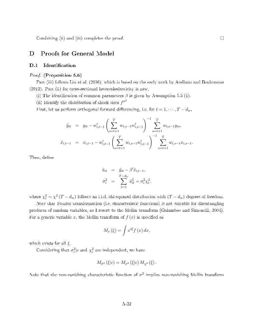
Combining (ii) and (iii) completes the proof.

D Proofs for General Model

D.1 Identication

Proof. (Proposition 5.6)

Part (iii) follows Liu et al. (2016), which is based on the early work by Arellano and Bonhomme

(2012). Part (ii) for cross-sectional heteroskedasticity is new.

(i) The identication of common parameters β is given by Assumption 5.5 (1).

(ii) Identify the distribution of shock sizes fσ2

First, let us perform orthogonal forward dierencing, i.e. for t = 1, · · · , T − dw,

yit = yit − w′i,t−1

(T∑

s=t+1

wi,s−1w′i,s−1

)−1 T∑s=t+1

wi,s−1yis,

xi,t−1 = xi,t−1 − w′i,t−1

(T∑

s=t+1

wi,s−1w′i,s−1

)−1 T∑s=t+1

wi,s−1xi,s−1.

Then, dene

uit = yit − β′xi,t−1,

σ2i =

T−dw∑t=1

u2it = σ2

i χ2i .

where χ2i ∼ χ2 (T − dw) follows an i.i.d. chi-squared distribution with (T − dw) degrees of freedom.

Note that Fourier transformation (i.e. characteristic functions) is not suitable for disentangling

products of random variables, so I resort to the Mellin transform (Galambos and Simonelli, 2004).

For a generic variable x, the Mellin transform of f (x) is specied as

Mx (ξ) =

ˆxiξf (x) dx,

which exists for all ξ.

Considering that σ2i |c and χ2

i are independent, we have

Mσ2 (ξ|c) = Mσ2 (ξ|c)Mχ2 (ξ) .

Note that the non-vanishing characteristic function of σ2 implies non-vanishing Mellin transform

A-22

Mσ2 (ξ|c) (almost everywhere), so it is legitimate to take the logarithm of both sides,

logMσ2 (ξ|c) = logMσ2 (ξ|c) + logMχ2 (ξ) .

Taking the second derivative with respect to ξ, we get

∂2

∂ξ∂ξ′logMσ2 (ξ|c) =

∂2

∂ξ∂ξ′logMσ2 (ξ|c)− ∂2

∂ξ∂ξ′logMχ2 (ξ) .

The Mellin transform of chi-squared distribution Mχ2 (ξ) is a known functional form. In addition,

we have

logMσ2 (0|c) = logMσ2 (0|c)− logMχ2 (0) = 0,

∂

∂ξlogMσ2 (0|c) =

∂

∂ξlogMσ2 (0|c)− ∂

∂ξlogMχ2 (0)

= i(E(

log σ2∣∣ c)− E

(χ2∣∣ c)) .

Based on Pav (2015),

E(χ2∣∣ c) = log 2 + ψ

(T − dw

2

),

where ψ (·) is the derivative of the log of the Gamma function.Given logMσ2 (0|c), ∂

∂ξ logMσ2 (0|c), and ∂2

∂ξ∂ξ′ logMσ2 (ξ|c), we can fully recover logMσ2 (ξ|c)and hence uniquely determine fσ

2. Please refer to Theorem 1.19 in Galambos and Simonelli (2004)

for the uniqueness.

(iii) Identify the distribution of individual eects fλ

Dene

yi,1:T = yi,1:T − β′xi,0:T−1 = λ′iwi,0:T−1 + ui,1:T .

Let Y = yi,1:T , W = w′i,0:T−1, Λ = λi and U = ui,1:T . The above expression can be simplied as

Y = WΛ + U.

Denote FY , FΛ and FU as the conditional characteristic functions for Y , Λ and U , respectively.

Based on Assumption (5.5) (4), FΛ and FU are non-vanishing almost everywhere. Then, we obtain

logFΛ

(W ′ξ|c

)= logFY (ξ|c)− logFU (ξ|c) .

Let ζ = W ′ξ and AW = (W ′W )−1W ′, then the second derivative of logFΛ (ζ|c) is characterized by

∂2

∂ζ∂ζ ′logFΛ (ζ|c) = AW

(∂2

∂ξ∂ξ′(logFY (ξ|c)− logFU (ξ|c)

))A′W .

A-23

Moreover,

logFΛ (0|c) = 0,

∂

∂ζlogFΛ (0|c) = iE

(AW Y

∣∣∣ c) ,so we can pin down log Λ (ζ|c) and fλ.

The proof of Proposition (5.8) for unbalanced panels follows in a similar manner.

D.2 Cross-sectional Heteroskedasticity

Proof. (Proposition 5.9)

(i) KL requirement

As λ and σ2 are independent, we have

dKL

(fλ0 f

σ2

0 , fλfσ2)

= dKL

(fλ0 , f

λ)

+ dKL

(fσ

2

0 , fσ2).

Based on the observed sucient statistics λ = 1T

∑Tt=1 yit with corresponding errors u = 1

T

∑Tt=1 uit,

the KL requirement is: for all ε > 0,

Π

f ∈ F , fσ2 ∈ Fσ2

::

ˆfλ0

(λ− u

)φ

(u; 0,

σ2

T

)fσ

2

0

(σ2)

log

´fλ0

(λ− u′

)φ(u; 0, σ

2′

T

)fσ

2

0

(σ2′) du′dσ2′

´fλ(λ− u′

)φ(u; 0, σ

2′

T

)fσ2 (σ2′) du′dσ2′

· dudσ2dλ < ε

> 0.

As in the proof of Proposition 4.7 part (i), similar convexity reasoning can be applied to bound the

KL divergence on y by dKL

(fλ0 f

σ2

0 , fλfσ2). The sucient conditions for KL properties on λ and

l are listed in Lemmas 4.8 and E.1. Note that since the KL divergence is invariant under variable

transformations, the KL property of the distribution of l is equivalent to the KL property of the

distribution of σ2.

(ii) Uniformly exponentially consistent tests

The alternative region can be split into the following two parts:

(ii-a) fσ2 ∈ U cε′,Φ′

(fσ

2

0

)Orthogonal forward dierencing yields yit ∼ N

(0, σ2

i

). Dene σ2

i =∑T−dw

t=1 y2it = σ2

i χ2i , where

χ2i ∼ χ2 (T − dw) follows an i.i.d. chi-squared distribution with (T − dw) degrees of freedom. Here

and below, I ignore the subscripts to simplify the notation.

Let gσ2 (σ2)

= fσ2 (σ2)− fσ2

0

(σ2). There are always tests if we observe σ2, then for any gσ

2,

A-24

there exists a ε > 0 such that ˆ ∣∣∣gσ2 (σ2)∣∣∣ dσ2 > ε. (D.1)

Similar to part (ii-b) in the proof of Proposition 4.7, here again I utilize the proof-by-contradiction

technique. Suppose there is no test when σ2 is observed instead of σ2, then there exist a gσ such

that

h(σ2)

=

ˆgσ

2

(σ2

χ2

)fχ2

(χ2)dχ2 = 0 for all σ2,

due to the continuity of h. Here I utilize the Mellin transform for products of random variables. As

σ2 and χ2 are independent, we have

Mσ2 (ξ) = Mσ2 (ξ) ·Mχ2 (ξ) = 0 for all ξ.

The Mellin transform of chi-squared distribution Mχ2 (ξ) 6= 0, then

Mσ2 (ξ) = 0 for all ξ.

Note that Mσ2 (ξ) uniquely determines gσ2 (σ2). Then, the inverse Mellin transform leads to

gσ2 (σ2)

= 0 for all σ2,

which contradicts equation (D.1). Therefore, there are also tests distinguishing the true fσ2

0 from

alternative fσ2even when we only observe σ2.

(ii-b') fσ2

= fσ2

0 , fλ ∈ U cε,Φ(fλ0)

This is an intermediate step for part (ii-c). Once again I resort to proof by contradiction. Dene

gλ (λ) = fλ (λ)−fλ0 (λ). There are always tests if we observe λ, then for any gλ, there exists a ε > 0

such that ˆ ∣∣∣gλ (λ)∣∣∣ dλ > ε. (D.2)

Suppose there is no test when y is observed instead of λ, then there exist a gλ such that

0 = h (y) =

ˆgλ (y − u)φ

(u; 0, σ2

)fσ

2

0

(σ2)dudσ2 for all y

=⇒0 = Fy (ξ) =

ˆe−iξy gλ (y − u)φ

(u; 0, σ2

)fσ

2

0

(σ2)dudσ2dy

=

ˆe−iξ(λ+σv)gλ (λ)φ

(u; 0, σ2

)fσ

2

0

(σ2)dudσ2dλ

= Fλ (ξ) ·ˆc1 exp

(−c2ξ

2σ2)fσ

2

0

(σ2)dσ2 = 0 for all ξ

=⇒Fλ (ξ) = 0 for all ξ

=⇒gλ (λ) = 0 for all λ,

A-25

which contradicts equation (D.2). Therefore, there are also tests if we know fσ2

0 but only observe y.

(ii-b) fσ2 ∈ Uε′,Φ′

(fσ

2

0

), fλ ∈ U cε,Φ

(fλ0)

Without loss of generality, let Φ = ϕ and ϕ? be the corresponding test function when fσ2

0 is

known as in case (ii-b'). Then, the dierence between Ef (ϕ?) and Ef0 (ϕ?) is

ˆϕ?(λ)fλ(λ− u

)φ

(u; 0,

σ2

T

)fσ

2 (σ2)dudσ2dλ−

ˆϕ?(λ)fλ0

(λ− u

)φ

(u; 0,

σ2

T

)fσ

2

0

(σ2)dudσ2dλ

>

ˆϕ?(λ)(

fλ(λ− u

)− fλ0

(λ− u

))φ

(u; 0,

σ2

T

)fσ

2

0

(σ2)dudσ2dλ

−∣∣∣∣ˆ ϕ?

(λ)fλ(λ− u

)φ

(u; 0,

σ2

T

)(fσ

2 (σ2)− fσ2

0

(σ2))dudσ2dλ

∣∣∣∣ .Case (ii-b') implies that the rst term is greater than some ε > 0. Meanwhile, we can choose

ε′ = ε/2 and Φ′ =ϕ′(σ2)

= 1for Uε′,Φ′

(fσ

2

0

)so that the second term is bounded by ε/2. Hence,

Ef (ϕ?) − Ef0 (ϕ?) > ε/2, and ϕ? is the test function with respect to the alternative sub-regionfσ

2 ∈ Uε′,Φ′(fσ

2

0

), fλ ∈ U cε,Φ

(fλ0)

.

E Extension: Heavy Tails

Lemma E.1 gives one set of conditions accommodating fz0 with heavy tails using the Gaussian-

mixture DPM prior. It follows Tokdar (2006) Theorem 3.3. The notation is slightly dierent from

Tokdar (2006). Here Gz0 is dened on(µzi , (ω

zi )

2), the mean and the variance, while Tokdar (2006)

has the mean and the standard deviation as the arguments for Gz0.

Lemma E.1. (Tokdar, 2006)

If fz0 and the DP base distribution Gz0 satisfy the following conditions:

1.∣∣´ fz0 (z) log fz0 (z) dz

∣∣ <∞.

2. For some η ∈ (0, 1),´|z|η fz0 (z) dz <∞.

3. There exist ω0 > 0, 0 < b1 < η, b2 > b1, and c1, c2 > 0 such that for large µ > 0,

max

Gz0

([µ− ω0µ

η2 ,∞

)×[ω2

0,∞)), Gz0

([0,∞)×

(µ2−η,∞

)),

Gz0

((−∞,−µ+ ω0µ

η2

]×[ω2

0,∞)), Gz0

((−∞, 0]×

(µ2−η,∞

)) ≥ c1µ

−b1 ,

max

Gz0 ((−∞, µ)× (0, exp (2µη − 1))) ,

Gz0 ((−µ,∞)× (0, exp (2µη − 1)))

> 1− c2µ

−b2 .

Then, fz0 ∈ KL (Πz).

The next lemma extends Lemma E.1 to the multivariate case. Then, Proposition E.3 largely parallels

Proposition (5.10) with dierent condition sets for the KL property, which accounts for heavy tails

in the true unknown distributions..

A-26

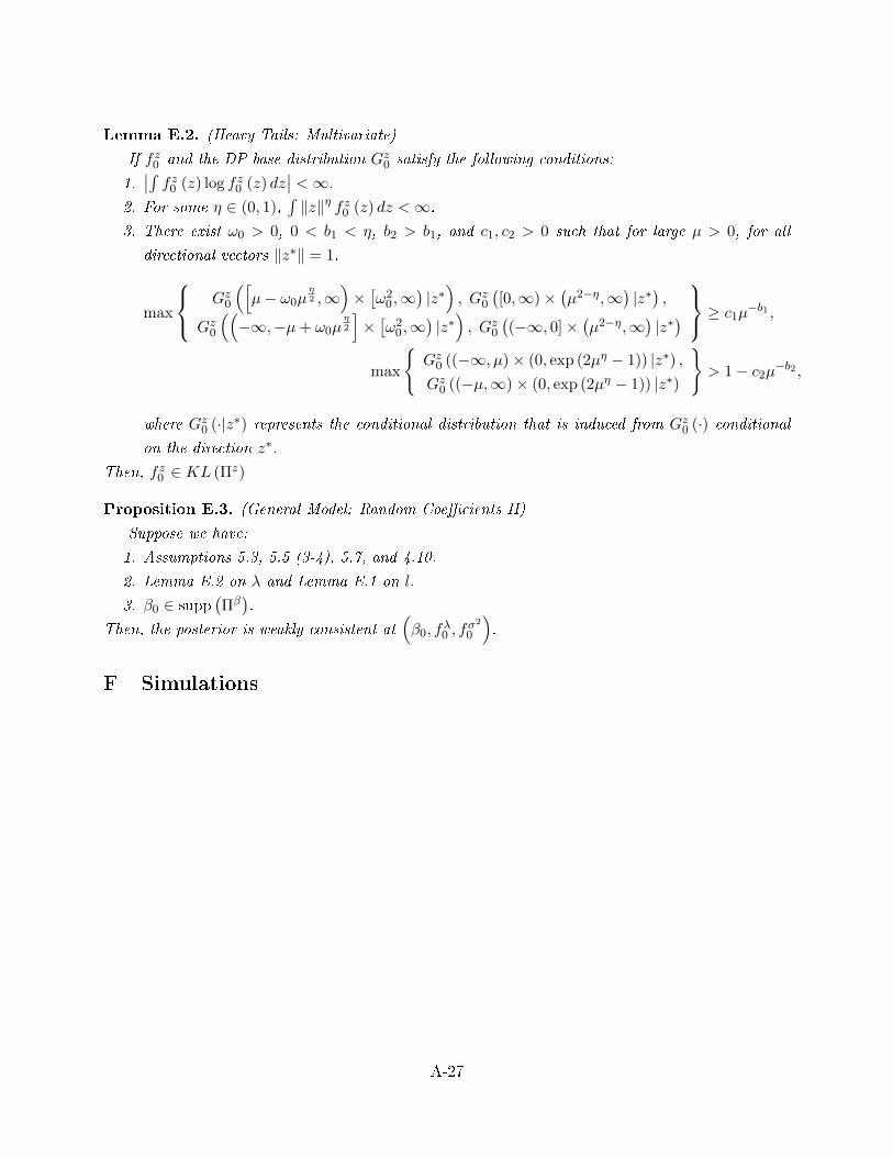
Lemma E.2. (Heavy Tails: Multivariate)

If fz0 and the DP base distribution Gz0 satisfy the following conditions:

1.∣∣´ fz0 (z) log fz0 (z) dz

∣∣ <∞.

2. For some η ∈ (0, 1),´‖z‖η fz0 (z) dz <∞.

3. There exist ω0 > 0, 0 < b1 < η, b2 > b1, and c1, c2 > 0 such that for large µ > 0, for all

directional vectors ‖z∗‖ = 1,

max

Gz0

([µ− ω0µ

η2 ,∞

)×[ω2

0,∞)|z∗), Gz0

([0,∞)×

(µ2−η,∞

)|z∗),

Gz0

((−∞,−µ+ ω0µ

η2

]×[ω2

0,∞)|z∗), Gz0

((−∞, 0]×

(µ2−η,∞

)|z∗) ≥ c1µ

−b1 ,

max

Gz0 ((−∞, µ)× (0, exp (2µη − 1)) |z∗) ,Gz0 ((−µ,∞)× (0, exp (2µη − 1)) |z∗)

> 1− c2µ

−b2 ,

where Gz0 (·|z∗) represents the conditional distribution that is induced from Gz0 (·) conditional

on the direction z∗.

Then, fz0 ∈ KL (Πz)

Proposition E.3. (General Model: Random Coecients II)

Suppose we have:

1. Assumptions 5.3, 5.5 (3-4), 5.7, and 4.10.

2. Lemma E.2 on λ and Lemma E.1 on l.

3. β0 ∈ supp(Πβ).

Then, the posterior is weakly consistent at(β0, f

λ0 , f

σ2

0

).

F Simulations

A-27

Figure F.1: Convergence Diagnostics: β

For each iteration s, rolling mean is calculated over the most recent 1000 draws.

A-28

Figure F.2: Convergence Diagnostics: σ2

For each iteration s, rolling mean is calculated over the most recent 1000 draws.

A-29

Figure F.3: Convergence Diagnostics: α

For each iteration s, rolling mean is calculated over the most recent 1000 draws.

A-30

Figure F.4: Convergence Diagnostics: λ1

For each iteration s, rolling mean is calculated over the most recent 1000 draws.

A-31

Figure F.5: f0 vs Π (f | y1:N,0:T ) : Baseline Model, N = 105

The black solid line represents the true λi distribution, f0. The blue bands show the posterior distributionof f , Π (f | y1:N,0:T ).

A-32