Evaluating Density ForecastsFrancis X. Diebold , Todd A. Gunther , and Anthony S. Tay* # +

Department of Economics*

University of Pennsylvaniaand

NBER

Department of Economics#

University of Pennsylvania

Department of Economics and Statistics+

National University of Singapore

This Print: August 23, 1997

Send correspondence to Diebold at fdiebold@mail.sas.upenn.edu.

Copyright © 1997 F.X. Diebold, T.A. Gunther, and A.S. Tay. This paper is available on theWorld Wide Web at http://www.ssc.upenn.edu/~diebold/ and may be freely reproduced foreducational and research purposes, so long as it is not altered, this copyright notice isreproduced with it, and it is not sold for profit.

Abstract: We propose methods for evaluating density forecasts. We focus primarily onmethods that are applicable regardless of the particular user’s loss function. We illustrate themethods with a detailed simulation example, and then we present an application to densityforecasting of daily stock market returns. We discuss extensions for improving suboptimaldensity forecasts, multi-step-ahead density forecast evaluation, multivariate density forecastevaluation, monitoring for structural change and its relationship to density forecasting, anddensity forecast evaluation with known loss function.

Acknowledgments: Thorough reading and comments from two referees and Ken Westdrastically improved this paper. Helpful discussion was also provided by seminar participantsat Harvard/MIT, Michigan, Penn, Princeton, the Federal Reserve Bank of Kansas City, theFederal Reserve Bank of Atlanta, and the UCSD Conference on Time Series Analysis ofHigh-Frequency Financial Data. We are especially grateful for helpful comments from GaryChamberlain, Clive Granger, Jin Hahn, Bruce Hansen, Jerry Hausman, Hashem Pesaran, JimStock, Ken Wallis, Mark Watson and Tao Zha. All remaining inadequacies are ours alone. For support we thank the National Science Foundation, the Sloan Foundation, the Universityof Pennsylvania Research Foundation, and the National University of Singapore.

Diebold, F.X., Gunther, T. and Tay, A. (1998), "Evaluating Density Forecasts, with Applications to Financial Risk Management,"

International Economic Review, 39, 863-883.

See, for example, Efron and Tibshirani (1993) and Gelman, Carlin, Stern and Rubin1

(1995).

2

1. Introduction

Prediction occupies a distinguished position in econometrics; hence, evaluating

predictive ability is a fundamental concern. Reviews of the forecast evaluation literature,

such as Diebold and Lopez (1996), reveal that most attention has been paid to evaluating

point forecasts. In fact, the bulk of the literature focuses on point forecasts, while

conspicuously smaller sub-literatures treat interval forecasts (e.g., Chatfield, 1993;

Christoffersen, 1997) and probability forecasts (e.g., Wallis, 1993; Clemen, Murphy and

Winkler, 1995).

Little attention has been given to evaluating density forecasts. At least three factors

explain this neglect. First, analytic construction of density forecasts has historically required

restrictive and sometimes dubious assumptions, such as Gaussian innovations and no

parameter estimation uncertainty. Recent work using numerical and simulation techniques to

construct density forecasts, however, has reduced our reliance on such assumptions. In fact,

improvements in computer technology have rendered the provision of credible density

forecasts increasingly straightforward, in both classical and Bayesian frameworks. 1

Second, until recently there was little demand for density forecasts; historically, point

and interval forecasts seemed adequate for most users' needs. Again, however, recent

developments have changed the status quo, particularly in quantitative finance. The booming

area of financial risk management, for example, is effectively dedicated to providing density

forecasts of portfolio values and to tracking certain aspects of the densities. The day will soon

3

arrive in which risk management will routinely entail nearly real -time issuance and evaluation

of such density forecasts.

Finally, the problem of density forecast evaluation appears difficult. Although it is

possible to adapt techniques developed for the evaluation of point, interval and probability

forecasts to the evaluation of density forecasts, such approaches lead to incomplete evaluation

of density forecasts. For example, using Christoffersen’s (1997) method for evaluating

interval forecasts, we can evaluate whether the series of 90% prediction intervals

corresponding to a series of density forecasts is correctly conditionally calibrated, but that

leaves open the question of whether the corresponding prediction intervals at other confidence

levels are correctly conditionally calibrated. Correct conditional calibration of density

forecasts corresponds to the simultaneous correct conditional calibration of all possible

interval forecasts, the assessment of which seems a daunting task.

In light of the increasing importance of density forecasts, and lack of attention paid to

them in the literature, we propose methods for evaluating density forecasts. Our work is

related to the contemporaneous and independent work of Granger and Pesaran (1996), who

explore a decision environment with probability forecasts defined over discrete outcomes (an

environment different from ours, but closely related), and obtain a result analogous to our

Proposition 2. They do not, however, focus on forecast evaluation. Our evaluation methods

are based on an integral transform that turns out to have a long history, dating at least to

Rosenblatt (1952). Contemporaneous and independent work by Crnkovic and Drachman

(1996) is also closely related.

4

We proceed as follows. In section 2, we present a detailed statement and discussion of

the problem, and we provide the theoretical underpinnings of the methods that we introduce

subsequently. In section 3 we present methods of density forecast evaluation when the loss

function is not known, which is often the relevant case in practice. In section 4, we provide a

detailed simulation example of density forecast evaluation in an environment with time-

varying volatility. In section 5, we use our tools to evaluate density forecasts of U.S. S&P

500 daily stock returns. In section 6, we discuss extensions for improving suboptimal density

forecasts, evaluating multi-step and multivariate density forecasts, monitoring for structural

change when density forecasting, and evaluating density forecasts when the loss function is

known. We conclude in section 7.

2. Density Forecasts, Loss Functions and Action Choices: Implications for Density

Forecast Evaluation

Studying the relationships among density forecasts, loss functions and action choices

will help to clarify what can and can not be hoped for when evaluating density forecasts, and

will suggest productive directions for density forecast evaluation. We first show that the

problem of density forecast evaluation is intrinsically linked to the forecast user’s loss

function, which would appear to bode poorly for our quest for a universally-applicable

approach to density forecast evaluation. We then show that, contrary to first impressions, all

is not lost: the analysis suggests an important route to density forecast evaluation, which we

pursue in subsequent sections.

The Decision Environment

ft (yt) pt (yt) t

a (p(y)) argmina A

L(a, y)p(y)dy .

{ft (yt | t )}mt 1 yt

t {yt 1 , yt 2 , ... } {pt(yt | t)}mt 1

{yt}mt 1

L(a, y)

p(y)

a

L(a , y)

y f(y)

For notational convenience, we will often not indicate the information set and simply2

write and , but the dependence on should be understood. Moreover, becausein this section we consider the relationships among density forecasts, loss functions andactions in a one-period context, we temporarily drop the time subscripts for notationalconvenience.

We indulge in the standard abuse of notation, which favors convenience over3

precision, by failing to distinguish between random variables and their realizations. Themeaning will be clear from context.

Note the implicit assumption that agents proceed as if p equals f, in spite of the fact4

that p is only an estimate of f. A richer analysis would account for the estimationuncertainty; see the concluding remarks at the end of this paper.

We assume a unique minimizer. A sufficient condition is that A be compact and that5

L be strictly convex in ‘a’.

5

Let be the sequence of data generating processes governing a series ,

where , and let be a corresponding sequence of 1-step-

ahead density forecasts. Finally, let denote the corresponding series of realizations.2 3

Each forecast user has a loss function , where ‘a’ refers to an action choice,

and chooses an action to minimize expected loss computed using the density believed to be

the data generating process. If she believes that the density forecast is the correct4

density, then she chooses an action such that5

The action choice defines the loss faced for every realization of the process

. This loss is a random variable and possesses a probability distribution, which we

call the loss distribution, and which depends only on the action choice.

Expected loss with respect to the true data generating process is

E[L(a , y)] L(a , y) f(y)dy.

L(a j , y) f(y)dy L(ak , y) f(y)dy,

rj rk L(aj ,y)f(y)dy L(ak ,y)f(y)dy .

pj (y) pk (y)

pj (y) pk (y)

aj

f(y) y aj

pj ak pk

pj pk

L(a, y)

6

The effect of the density forecast on the user’s expected loss is easily seen. A density forecast

translates into a loss distribution. Two different forecasts will, in general, lead to different

action choices and hence different loss distributions. The better is a density forecast, the

lower is its expected loss, computed with respect to the true data generating process.

Ranking Two Forecasts

Suppose the user has the option of choosing between two forecasts in a given period,

denoted by and , where the subscript refers to the forecast. The user will weakly

prefer forecast to forecast if

where denotes the action that minimizes expected loss when the user bases the action

choice on forecast j.

Ideally, we would like to find a ranking of forecasts with which all users would agree,

regardless of their loss function. Unfortunately, the following proposition shows that such a

ranking does not exist.

Proposition 1: Let be the density of , let be the optimal action based on forecast

, and let be the optimal action based on forecast . Then there does not exist a ranking

r of arbitrary density forecasts and , both distinct from f, such that for all loss functions

,

L1(ak , y) f(y)dy < L1(aj ,y)f(y)dy,

L2(ak , y) f(y)dy > L2(aj ,y)f(y)dy.

L1

L2 pj pk

L1(a, y) (y a)2

L2(a, y) (y 2 a)2 y p(y) dy

y 2 p(y) dy

The result is analogous to Arrow's celebrated impossibility theorem. The ranking6

effectively reflects a social welfare function, which does not exist.

7

Proof: In order to establish the result, it is sufficient to find a pair of loss functions and

, a density function f governing y, and a pair of forecasts, and , such that

while

That is, user 1 does better on average under forecast k, while user 2 does better under forecast

j. It is straightforward to construct such an example. Suppose the true density function is

N(0,1), and suppose that user 1's loss function is and user 2's loss

function is . The optimal action choices are then and

. That is, user 1 bases her action choice on the mean, with higher expected loss

occurring with larger errors in the forecast mean, while user 2's actions and expected losses

depend on the error in the forecast of the uncentered second moment. In this context,

consider two forecasts: forecast j is N(0,2) and forecast k is N(1,1). User 1 prefers forecast j,

because it leads to an action choice, and hence a loss distribution, with lower expected loss,

but user 2 prefers forecast k for the same reason.

To repeat: there is no way to rank two incorrect density forecasts such that all users

will agree with the ranking. However, it is easy to see that if a forecast coincides with the6

L(a j , y) f(y)dy L(ak , y) f(y)dy, k.

pj (y) f(y) aj

aj

{p t (yt | t)}mt 1

{ft (yt | t )}mt 1

{p t (yt | t)}mt 1 {ft (yt | t )}m

t 1

{ft (yt | t )}mt 1

ft (yt t)

Granger and Pesaran (1996) independently arrive at a similar result.7

8

true data generating process, then it will be preferred by all forecast users, regardless of loss

function. Formally, we have the following proposition: 7

Proposition 2: Suppose that , so that minimizes the expected loss with

respect to the true distribution. Then

Proof: The result follows immediately from the assumption that minimizes expected loss

over all possible actions, including those which might be chosen under alternative density

forecasts.

The proposition, although simple, is not vacuous. In particular, it suggests a useful

direction for evaluating density forecasts. Regardless of loss function, we know that the

correct density is weakly superior to all forecasts, which suggests evaluating forecasts by

assessing whether the forecast densities are correct, i.e., whether =

. If not, we know that some users, depending on their loss functions, could

potentially be better served by a different density forecast. We now develop that idea in

detail.

3. Evaluating Density Forecasts

The task of determining whether = appears difficult,

perhaps hopeless, because is never observed, even after the fact. Moreover,

and importantly, the true density may exhibit structural change, as indicated by its

z tyt pt (u)du

Pt (yt).

q t(zt )P 1

t (z t)zt

ft (P 1t (zt ))

ft(P 1t (zt ))

p t(P 1t (zt ))

.

ft (yt)

pt (yt)

zt

qt (z t)

ft (yt) yt pt (yt) yt

zt yt pt (yt)P 1

t (zt )zt

yt zt

pt (yt)P t(yt )

yt

yt P 1t (z t)

pt (yt) ft(yt ) qt (z t)

9

time subscript. As it turns out, the challenges posed by these subtleties are not

insurmountable.

The Probability Integral Transform

Our methods are based on the relationship between the data generating process, ,

and the sequence of density forecasts, , as related through the probability integral

transform, , of the realization of the process taken with respect to the density forecast. The

probability integral transform is defined as

The following lemma describes the distribution, , of the probability integral transform.

Lemma 1: Let be the true density of , let be a density forecast of , and let

be the probability integral transform of with respect to . Then assuming that

is continuous and nonzero over the support of , has support on the unit

interval with density

Proof: Follows from the facts that and .

Note, in particular, a key fact: if , then is simply the U(0,1) density.

This idea dates at least to Rosenblatt (1952).

{z t}mt 1

iidU(0,1).

q(z1,z2, ...,zm)

y1

z1

...y1

zm

ym

z1

...ym

zm

fm(P 1m (zm) | m) fm 1(P 1

m 1(zm 1 ) | m 1) ...

...× f1(y 11 (z1 ) | 1 )

y1

z1

y2

z2

ym

zm

fm(P 1m (zm) | m) fm 1(P 1

m 1(zm 1 ) | m 1) ...

...×f1 (y 11 (z1) | 1),

pt (yt) ft(yt )

pt (yt) ft(yt )

{yt}mt 1 {ft (yt | t)}m

t 1

t {yt 1 , yt 2 , ... } {p t (yt)}mt 1

{ft (yt | t)}mt 1

{yt}mt 1

{p t (yt)}mt 1

{yt}mt 1

f(ym , ... ,y1 | 1) fm(ym | m) fm 1 (ym 1 | m 1 ) ... f1(y1 | 1 ).

{z t}mt 1

10

Now we go beyond our one-period characterization of the density of z when

and characterize both the density and dependence structure of the entire z

sequence when .

Proposition 3: Suppose is generated from where

. If a sequence of density forecasts coincides with

, then under the usual condition of a non-zero Jacobian with continuous partial

derivatives, the sequence of probability integral transforms of with respect to

is iid U(0,1). That is,

Proof: The joint density of can be decomposed as

We therefore compute the joint density of using the change of variables formula

because the Jacobian of the transformation is lower triangular. Thus we have

q(zm, ... , z1 | )fm(P 1

m (zm) | m)

pm(P 1m (zm))

.fm 1(P 1

m 1 (zm 1) | m 1)

pm 1(P 1m 1 (zm 1))

...

...×f1(P 1

1 (z1) | 1)

p1 (P 11 (z1 ))

.

{z t}mt 1

{z t}mt 1

{zt}mt 1

The “hit” series is 1 if the realization is contained in the forecast interval, and 08

otherwise.

11

From Lemma 1, under the assumed conditions, each of the ratios above is a U(0,1) density,

the product of which yields an m-variate U(0,1) distribution for . Because the joint

distribution is the product of the marginals, we have that is distributed iid U(0,1).

The intuition for the above result may perhaps be better understood from the

perspective of Christoffersen (1997), who shows that a correctly conditionally calibrated

interval forecast will provide a hit sequence that is distributed iid Bernoulli, with the desired

success probability. If a sequence of density forecasts is correctly conditionally calibrated,8

then every interval will be correctly conditionally calibrated and will generate an iid Bernoulli

hit sequence. This fact manifests itself in the iid uniformity of the corresponding probability

integral transforms.

Practical Application

The theory developed thus far suggests that we evaluate density forecasts by assessing

whether the probability integral transform series, , is iid U(0,1). Simple tests of iid

U(0,1) behavior are readily available, such as runs tests or Kolmogorov-Smirnov tests, all of

12

which are actually joint tests of uniformity and iid. Such tests, however, are not likely to be

of much value in practical applications, because they are not constructive; that is, when

rejection occurs, the tests generally provide no guidance as to why. If, for example, such a

statistic rejects the hypothesis of iid U(0,1) behavior, is it because of violation of

unconditional uniformity, violation of iid, or both? Moreover, even if we know that rejection

comes from violation of uniformity, we’d like to know more: What, precisely, is the nature of

the violation of uniformity, and how important is it? Similarly, even if we know that rejection

comes from a violation of iid, what precisely is its nature? Is z heterogeneous but

independent, or is z dependent? If z is dependent, is the dependence operative primarily

through the conditional mean, or are higher-ordered conditional moments, such as the

variance, relevant? Is the dependance strong and important, or is iid an adequate

approximation, even if strictly false?

The nonconstructive nature of tests of iid U(0,1) behavior, and the nonconstructive

nature of related separate tests of iid and U(0,1), make us eager to adopt more revealing

methods of exploratory data analysis. First, as regards evaluating unconditional uniformity,

we suggest visual assessment using the obvious graphical tool, a density estimate. Simple

histograms are attractive in the present context because they allow straightforward imposition

of the constraint that z has support on the unit interval, in contrast to more sophisticated

procedures such as kernel density estimates with the standard kernel functions. The estimated

density can be visually compared to a U(0,1), and confidence intervals under the null

hypothesis of iid U(0,1) are easy to compute.

yt

2ht

3t(6)

(z z ) ( z z )

(z z ) ( z z )2 ( z z )3 ( z z )4

A caveat, however, is that there is in general no one-to-one correspondence between9

the type of dependence found in z and the dependence in y missed by the forecasts.

13

Second, as regards evaluating whether z is iid, we again suggest visual assessment

using the obvious graphical tool, the correlogram, supplemented with the usual Bartlett

confidence intervals. The correlogram assists with the detection of particular dependence

patterns in z and can provide useful information about the deficiencies of density forecasts.

For instance, serial correlation in the z series may indicate that the mean dynamics have been

inadequately modeled by the forecaster. Because we’re interested in potentially sophisticated9

nonlinear forms of dependence, in addition to linear dependence, we examine not only the

correlogram of , but also those of powers of . In practice, we have found

examination of the correlograms of , , and to be adequate; it

will reveal dependence operative through the conditional mean, conditional variance,

conditional skewness, or conditional kurtosis.

4. Application to a Simulated GARCH Process

Before proceeding to apply our density forecast evaluation methods to real data, it is

useful to examine their efficacy on simulated data, for which we know the true data-

generating process. Hence we examine data simulated from a realistic t-GARCH process

designed to mimic high-frequency financial asset return data (Bollerslev, 1987). Specifically,

we use a GARCH(1,1) data generating process, the conditional density of which is a

standardized Student’s-t with six degrees of freedom,

ht y 2t 1 ht 1.

The process as specified does have mean zero and variance 1, but it is neither iid nor10

unconditionally Gaussian.

The dashed lines superimposed on the histogram are approximate 95% confidence11

intervals for the individual bin heights under the null that z is iid U(0,1).

14

We choose the parameters in accordance with those typically obtained when fitting GARCH

models to high-frequency financial asset returns: = 0.01, =0.13, and =0.86. We

simulate a series of length 8000, chosen to mimic the sample sizes typical of high-frequency

financial data, and we plot it in Figure 1. The persistence in conditional volatility is visually

obvious.

We will examine the usefulness of our density forecast evaluation methods in

assessing four progressively better density forecasts. Throughout, we split the sample in half

and use the “in-sample” observations 1 through 4000 for estimation, and the “out-of-sample”

observations 4001 through 8000 for density forecast evaluation.

To establish a benchmark, we first evaluate forecasts that are based on an incorrect and

extremely naive assumption that the process is iid N(0,1). That is, in each of the periods10

4001-8000, we simply issue the forecast “N(0,1).” In Figure 2a we show two histograms of z,

one with 20 bins and one with 40 bins. The histograms have a distinct non-uniform11

“butterfly” shape -- a hump in the middle and two wings on the sides -- indicating that too

many of the realizations fell in middle and in the tails of the forecast densities relative to what

we’d expect if the data were really iid normal. This is exactly what we’d hope the histograms

( z z ) ( z z )2 ( z z )3 ( z z )4

( z z )2 ( z z )4

The dashed lines superimposed on the correlograms are Bartlett’s approximate 95%12

confidence intervals under the null that z is iid.

15

to reveal, given that the data-generating process is an unconditionally leptokurtic

GARCH(1,1).

In Figure 2b we show the correlograms of , , and . 12

The strong serial correlation in and makes clear another key deficiency of

the N(0,1) forecasts -- they fail to capture the volatility dynamics operative in the process.

Again, this is what we’d hope the correlograms would reveal, given our knowledge of the true

data-generating process.

Second, we evaluate forecasts produced under the incorrect assumption that the

process is iid but not necessarily Gaussian. We estimate the unconditional distribution from

observations 1 through 4000, freeze it, and then issue it as the density forecast in each of the

periods 4001 through 8000. Figures 3a and 3b contain the results. The z histogram is now

almost perfect (as it must be, apart from estimation error, which is small in a sample of size

4000), but the correlograms correctly continue to indicate neglected volatility dynamics.

Third, we evaluate forecasts that are based on a GARCH(1,1) model estimated under

the incorrect assumption that the conditional density is Gaussian. We use observations 1

through 4000 to estimate the model, freeze the estimated model, and then use it to make

(time-varying) density forecasts from 4001 through 8000. Figures 4a and 4b contain the z

histograms and correlograms. The histograms are closer to uniform and therefore improved,

but they still display slight peaks at either end and a hump in the middle. We would hope to

see such a reduction, but not elimination, of the butterfly pattern, because allowance for

Recall that the data generating process is conditionally, as well as unconditionally,13

fat-tailed.

16

conditionally Gaussian GARCH effects should account for some, but not all, unconditional

leptokurtosis. The correlograms now show no evidence of neglected conditional volatility13

dynamics, again as expected because the conditionally Gaussian GARCH model delivers

consistent estimates of the conditional variance parameters, in spite of the fact that the

conditional density is misspecified (Bollerslev and Wooldridge, 1992).

Finally, we forecast with an estimated correctly-specified t-GARCH(1,1) model. We

show the z histogram and correlograms in Figures 5a and 5b. Because we are forecasting

with a correctly specified model, estimated using a large sample, we would expect that the

histogram and the correlograms would fail to find flaws with the density forecasts, which is

the case.

In closing this section, we note that at each step of the above simulation exercise, our

density forecast evaluation procedures clearly and correctly revealed the strengths and

weaknesses of the various density forecasts. The results, as with all simulation results, are

specific to the particular data-generating process examined, but the process and the sample

size were chosen to be realistic for the leading applications in high-frequency finance. This

gives us confidence that the procedures will perform well on real financial data, to which we

now turn, and for which we don’t have the luxury of knowing the true data-generating

process.

5. Application to Daily S&P 500 Returns

( z z )2 ( z z )4

See, among many others, Bollerslev, Chou and Kroner (1992).14

17

We study density forecasts of daily value-weighted S&P 500 returns, with dividends,

from 02/03/62 through 12/29/95; we plot the data in Figure 6. As before, we split the sample

into in-sample and out-of-sample periods for model estimation and density forecast

evaluation. There are 4133 in-sample observations (07/03/62 - 12/29/78) and 4298 out-of-

sample observations (01/02/79 - 12/29/95). We then assess a series of density forecasts using

our evaluation methods.

As in the simulation example, we begin with an examination of N(0,1) density

forecasts, in spite of the fact that high-frequency financial data are well-known to be

unconditionally leptokurtic and conditionally heteroskedastic. In Figures 7a and 7b we14

show the histograms and correlograms of z. The histograms have the now-familiar butterfly

shape, indicating that the S&P realizations are leptokurtic relative to the N(0,1) density

forecasts, and the correlograms of and indicate that the N(0,1) forecasts are

severely deficient, because they neglect strong conditional volatility dynamics.

Next, we generate density forecasts using an apparently much more sophisticated

model. Both the Akaike and Schwarz information criteria select an MA(1)-GARCH(1,1)

model for the in-sample data, which we estimate, freeze, and use to generate out-of-sample

density forecasts. Figures 8a and 8b contain the z histograms and correlograms. The

histograms are closer to uniform and therefore improved, although they still display slight

peaks at either end and a hump in the middle. The correlograms look even better; all

evidence of neglected conditional volatility dynamics has vanished.

y

ym 1

Such a regression is sometimes called a Mincer-Zarnowitz regression, after Mincer15

and Zarnowitz (1969).

18

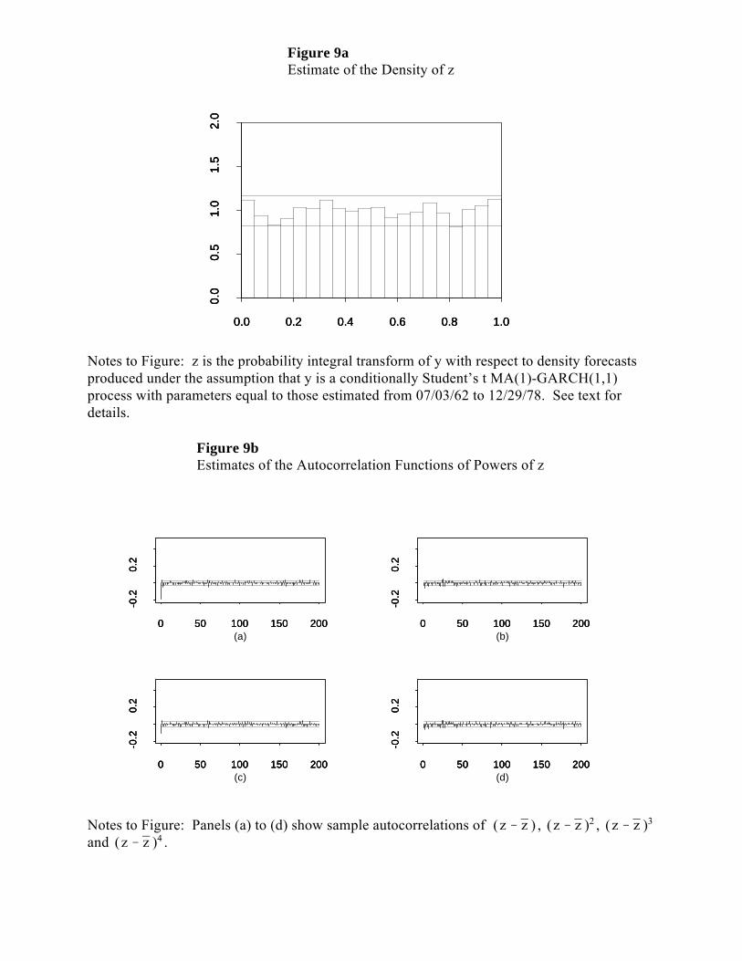
Finally, in an effort to remove the last vestiges of non-uniformity from the z

histogram, we estimate and then forecast with an MA(1) - t-GARCH(1,1) model. We show

the z histogram and correlograms in Figures 9a and 9b. The histogram is improved, albeit

slightly, and the correlograms remain good.

6. Extensions

Improving Density Forecasts

We have approached forecast evaluation from an historical perspective, evaluating the

ability of a forecaster based on past realizations. The intent, of course, is to gauge the likely

future accuracy of the forecaster based on past performance, assuming that the relationship

between the correct density and the forecaster’s predictive density remains fixed. Given that

we observe systematic errors in the historical forecasts, we may wish to simply reject the

forecast. It may also turn out that the errors are irrelevant to the user, a case we further

examine when we explicitly account for the user’s loss function. Nevertheless, it is possible

to take the errors into consideration when using the current forecast, just as it is possible to do

so in the point forecast case. In the point forecast case, for example, we can regress the y's on

the 's, the predicted values, and use the estimated relationship to construct an adjusted point

forecast.15

In the context of density forecasts that produce an iid z sequence, we can construct a

similar procedure by rewriting the relationship in Lemma 1. Suppose that the user is in period

m and possesses a density forecast of . From Lemma 1, we have

fm 1 (y m 1) pm 1(ym 1 ) qm 1 (P(ym 1 ))

pm 1(ym 1 ) qm 1 (zm 1).

qm 1 (z m 1) fm 1 (y m 1)

qm 1 (z m 1) qm 1 (z m 1)

{zt}mt 1 fm 1 (y m 1)

qm 1 (z m 1)

{z1, z3, z5, ... } {z2, z4, z6, ... }

In finite samples, of course, there is no guarantee that the “improved” forecast will16

actually be superior to the original, because it is based on an estimate of q rather than the trueq, and the estimate could be very poor. The same limitation obtains for Mincer-Zarnowitzregressions. The practical efficacy of our improvement methods is an empirical matter, whichwill have to await future research.

19

Thus if we know , we would know the actual distribution . Because

is unknown, an estimate can be formed using the historical series of

, and an estimate of the true distribution can then be constructed.

Standard density estimation techniques can be used to produce the estimate .16

Multi-Step-Ahead Density Forecasts

The evaluation of h-step ahead forecasts can also be evaluated using our methods,

except that provisions must be made for autocorrelation in z. This is analogous to expecting

MA(h-1) autocorrelation structures for optimal h-step ahead point forecast errors. In this

case, it will probably be easier to partition the z series into groups for which we expect iid

uniformity if the forecasts were indeed correct. For instance, for correct 2-step ahead

forecasts, the sub-series and should each be iid U(0,1), although

the full series would not be iid U(0,1).

If a formal test is desired, it may be obtained via Bonferroni bounds, as suggested in a

different context by Campbell and Ghysels (1995). Under the assumption that the z series is

(h-1)-dependent, each of the following h sub-series will be iid: {z , z , z , ...}, {z , z ,1 1+h 1+2h 2 2+h

z , ...}, ..., {z , z , z , ...}. Thus, a test with size bounded by can be obtained by2+2h h 2h 3h

performing h tests, each of size /h, on each of the h sub-series of z, and rejecting the null

p(y1t , y2t ,... , yNt | t 1) p(yNt | yN 1,t ,... , y1t , t 1) ... p(y2t | y1t , t 1 )p(y1t | t 1),

f(y1t , y2t ,... , yNt | t 1)N

i 1[p(yit | yi 1,t ,... , y1t , t 1) q(P(yit | yi 1,t ,... , y1t , t 1) )]

p(y1t , y2t ,... , yNt | t 1 ) q(z1t , z2t ,... , zNt | t 1) .

t 1 ( y1t , y2t ,..., yNt )

( y1t , y2t ,..., yNt )

20

hypothesis of iid uniformity if the null is rejected for any of the h sub-series. With the huge

high-frequency datasets now available in finance, such sample splitting, although inefficient,

is not likely to cause important power deterioration.

Multivariate Density Forecasts

The principle that governs the univariate techniques in this paper readily extends to the

multivariate case, as shown in Diebold, Hickman, Inoue and Tay (1997). Suppose that the

variable of interest y is now an (N x 1) vector, and that we have on hand m multivariate

forecasts and their corresponding multivariate realizations. Further suppose that we are able

to decompose each period’s forecasts into their conditionals, i.e., for each period’s forecasts

we can write

where now refers to the past history of . Then for each period we can

transform each element of the multivariate observation by its corresponding

conditional distribution. This procedure will produce a set of N z-series that will be iid U(0,1)

individually, and also when taken as a whole. Note that we will have N! sets of z series,

depending on how the joint density forecasts are decomposed, giving us a wealth of

information with which to evaluate the forecasts. In addition, the univariate formula for the

adjustment of forecasts, discussed above, can be applied to each individual conditional,

yielding

m

t 1zt N m

2, m

12,

m

t 1zt

m2

± 1.96 m12

.

m

t 1z 2

t N m3

, 4m45

,

m

t 1z 2

tm3

± 1.96 4m45

.

zt

iidU(0,1) zt

iid 12

, 112

z 2t

iid 13

, 445

21

Monitoring for Structural Change When Density Forecasting

Real-time monitoring of adequacy of density forecasts using CUSUM techniques is a

simple matter, because under the adequacy hypothesis the z series is iid U(0,1), which is free

of nuisance parameters. In particular, if , then , so that

asymptotically in m,

which yields the approximate 95% confidence interval for the CUSUM,

Similar calculations hold for the CUSUM of squares. Trivial calculations reveal that under

the adequacy hypothesis , so that asymptotically in m,

which yields the approximate 95% confidence interval for the CUSUM of squares,

Evaluating Density Forecasts Using a Specific Loss Function

If a series of density forecasts has been systematically in error, it may still be the case

that for a particular user, depending on her loss function, the systematic errors may be

ap af

dt L(ap,t , yt )1m

m

t 1L(ap,t , yt ).

ap

{pt(yt )}mt 1

{ap, t}mt 1

L(ap, t , yt )

Ef,t [L(af,t , yt )]

ap,t af, t

Ef,t [L(af,t , yt )]

Ep,t [L(ap,t , yt )] Ef,t [L(af,t , yt )]

Ef,t [L(af,t , yt )] Ep, t [L(ap, t af, t , yt )] E[dt ] 0

Because we have assumed a unique optimal action choice, .17

22

irrelevant. To be precise, the forecast may be such that the action choice induced by the

forecast, , minimizes the user’s actual expected loss. In such cases, which we now17

consider, the user’s loss function can be incorporated into the evaluation process, as is done in

other forecasting contexts by Diebold and Mariano (1995) and Christoffersen and Diebold

(1996, 1997a, 1997b).

Consider a density forecast series, , and the corresponding action series,

, of a particular user. The series of action choices results in a series of potential

losses, . We would like to compare each period’s realized loss with that period’s

expected loss under the optimal action choice . The expected difference will

be positive unless .

Unfortunately, we are unable to evaluate . Instead, we will have to use

an estimate of as a proxy for . We can then compute the

difference,

Under the joint null hypothesis that the series of density forecasts is optimal relative to the

user’s loss function and that the forecaster correctly specifies the expected loss in each period,

i.e., , we have , which can be tested in the

same way that Diebold and Mariano (1995) test whether two point forecasts are equally

accurate under the relevant loss function.

23

7. Summary and Concluding Remarks

We have provided a characterization of optimal density forecasts, and we have

proposed methods for evaluating whether reported density forecasts coincide with the true

sequence of conditional densities. In addition to studying the decision problem associated

with density forecasting and showing how to use the series of probability integral transforms

to judge the adequacy of a series of density forecasts, we also indicated how to improve a

suboptimal density forecast by using information on previously-issued density forecasts and

subsequent realizations, how to evaluate multi-step and multivariate density forecasts, and

how to monitor for structural change when density forecasting. We did all of this in a

framework not requiring specification of the loss function, but when information on the

relevant loss function is available, we also showed how to evaluate a density forecast with

respect to that loss function.

Notwithstanding their classical feel, our methods are also applicable to Bayesian

forecasts issued as predictive probability densities. Superficially, it would seem that strict

Bayesians would have little interest in our evaluation methods, on the grounds that

conditional on a particular sample path and specification of the prior and likelihood, the

predictive density simply is what it is, and there’s nothing to evaluate. But such is not the

case. A misspecified likelihood, for example, can lead to poor forecasts, whether classical or

Bayesian, and density forecast evaluation can help us to flag misspecified likelihoods. It

comes as no surprise, therefore, that model checking by comparing predictions to data is

emerging as an integral part of modern Bayesian data analysis and forecasting, as highlighted

For a concise introduction to predictive likelihood, see Bjørnstad (1990).18

We thank a clever referee for making this observation.19

24

for example in Gelman, Carlin, Stern and Rubin (1995), and our methods are very much in

that spirit.

It appears that our methods may also be related to the idea of predictive likelihood,

which is based not on the joint density of the sample (the likelihood), but rather the joint

density of future observations, conditional upon the sample (the predictive likelihood). 18 19

Moreover, in a fascinating development, Clements and Hendry (1993) establish a close link

between predictive likelihood and a measure of the accuracy of point forecasts that they

propose, the generalized forecast error second moment (GFESM). A more detailed

investigation of the relationships among our methods, predictive likelihood methods, and the

GFESM is beyond the scope of this paper but appears to be a promising direction for future

research.

In closing, we wish to focus on the fact that our evaluation tools do not depend on the

method used to produce the density forecasts being evaluated; in our framework, the forecasts

are the primitives, and in particular, we do not assume that the forecasts are based on a model.

This is useful because many density forecasts of interest do not come from models, and even

when they do, the forecast evaluator may not have access to the model. Such is the case, for

example, with the density forecasts of inflation recorded in the Survey of Professional

Forecasters since 1968; for a description of those forecasts and evaluation using our methods,

Diebold, Tay and Wallis also augment the methods proposed here with resampling20

procedures to approximate better the finite-sample distributions of the test statistics of interestin small macroeconomic, as opposed to financial, samples.

Our simulation results indicate that the effects of parameter estimation uncertainty21

are inconsequential at least for the comparatively large samples relevant in finance.

25

see Diebold, Tay and Wallis (1997). A second and very important example of model-free20

density forecasts is provided by the recent finance literature, which shows how to use options

written at different strike prices to extract a model-free estimate of the market’s risk-neutral

density forecast of returns on the underlying asset (e.g., Aït-Sahalia and Lo, 1995; Soderlind

and Svensson, 1997).

At the same time, we readily acknowledge that many density forecasts are based on

estimated models, and the sample size sometimes is small, in which case it seems clear that it

would be useful to extend our methods to account for parameter estimation uncertainty, in a

fashion precisely analogous to West’s (1996) and West and McCracken’s (1997) extensions

of Diebold and Mariano (1995). Similarly, the decision-theoretic background that we sketch21

requires that agents use density forecasts as if they were known to be the true conditional

density, in a fashion similar to West, Edison and Cho (1993); it remains to be seen how the

decision theory would change if uncertainty were acknowledged.

26

References

Aït-Sahalia, Y. and A. Lo (1995), “Nonparametric Estimation of State-Price Densities Implicitin Financial Asset Prices,” Manuscript, Graduate Schools of Business, Chicago andMIT.

Bjørnstad, J.F. (1990), “Predictive Likelihood: A Review,” Statistical Science, 5, 242-265.

Bollerslev, T. (1987), “A Conditional Heteroskedastic Time Series Model for SpeculativePrices and Rates of Return,” Review of Economics and Statistics, 69, 542-547.

Bollerslev, T., Chou, R.Y. and Kroner, K.F. (1992), “ARCH Modeling in Finance: A Reviewof the Theory and Empirical Evidence,” Journal of Econometrics, 52, 5-59.

Bollerslev, T. and Wooldridge, J.M. (1992), “Quasi-Maximum Likelihood Estimation andInference in Dynamic Models with Time-Varying Covariances,” EconometricReviews, 11, 143-179.

Campbell, B. and E. Ghysels (1995), “Federal Budget Projections: A NonparametricAssessment of Bias and Efficiency,” Review of Economics and Statistics, 77, 17-31.

Chatfield, C. (1993), “Calculating Interval Forecasts,” Journal of Business and EconomicsStatistics, 11, 121-135.

Christoffersen, P.F. (1997), “Evaluating Interval Forecasts,” International Economic Review,Forthcoming.

Christoffersen, P.F. and Diebold, F.X. (1996), “Further Results on Forecasting and ModelSelection Under Asymmetric Loss,” Journal of Applied Econometrics, 11, 561-572.

Christoffersen, P.F. and Diebold, F.X. (1997a), “Optimal Prediction Under AsymmetricLoss,” Econometric Theory, forthcoming. http://www.ssc.upenn.edu/~diebold/

Christoffersen, P.F. and Diebold, F.X. (1997b), “Cointegration and Long-HorizonForecasting,” Manuscript, Department of Economics, University of Pennsylvania. http://www.ssc.upenn.edu/~diebold/

Clemen, R.T., A.H. Murphy and R.L. Winkler (1995), “Screening Probability Forecasts: Contrasts Between Choosing and Combining,” International Journal of Forecasting,11, 133-146.

Clements, M.P. and Hendry, D.F. (1993), "On the Limitations of Comparing Mean SquareForecast Errors" (with discussion), Journal of Forecasting, 12, 617-637.

27

Crnkovic, C. and Drachman, J. (1996), “A Universal Tool to Discriminate Among RiskMeasurement Techniques,” Manuscript, J.P. Morgan & Co.

Diebold, F.X., Hickman, A., Schuermann, T. and Tay, A. (1997), “Evaluating MultivariateForex Density Forecasts,” Manuscript in preparation for Second Olsen Conference onHigh-Frequency Data in Finance. http://www.ssc.upenn.edu/~diebold/

Diebold, F.X. and J.A. Lopez (1996), “Forecast Evaluation and Combination,” in G.S.Maddala and C.R. Rao (eds.), Handbook of Statistics. Amsterdam: North-Holland,241-268.

Diebold, F.X. and R.S. Mariano (1995), “Comparing Predictive Accuracy,” Journal ofBusiness and Economic Statistics, 13, 253-263.

Diebold, F.X., Tay, A.S. and Wallis, K.D. (1997), “Evaluating Density Forecasts of Inflation: The Survey of Professional Forecasters,” in preparation for R.F. Engle and H. White(eds.), Festschrift in honor of C.W.J. Granger. http://www.ssc.upenn.edu/~diebold/

Efron, B. and Tibshirani, R.J. (1993), An Introduction to the Bootstrap. New York: Chapman and Hall.

Gelman, A, Carlin, J.B., Stern, H.S., Rubin, D.B. (1995), Bayesian Data Analysis. London: Chapman and Hall.

Granger, C.W.J. and M.H. Pesaran (1996), “A Decision Theoretic Approach to ForecastEvaluation,” Manuscript, Departments of Economics, University of California, SanDiego and Cambridge University.

Mincer, J. and V. Zarnowitz (1969), “The Evaluation of Economic Forecasts,” in J. Mincer(ed.), Economic Forecasts and Expectations. New York: National Bureau ofEconomic Research.

Rosenblatt, M. (1952), “Remarks on a Multivariate Transformation,” Annals of MathematicalStatistics, 23, 470-472.

Soderlind, P. and Svensson, L.E.O. (1997), “New Techniques to Extract Market Expectationsfrom Financial Instruments,” National Bureau of Economic Research Working Paper5877, Cambridge, Mass.

Wallis, K.F. (1993), Comment on J.H. Stock and M.W. Watson, “A Procedure for PredictingRecessions with Leading Indicators,” in J.H. Stock and M.W. Watson (eds.), BusinessCycles, Indicators and Forecasting. Chicago: University of Chicago Press for NBER,153-156.

28

West, K.D. (1996), "Asymptotic Inference About Predictive Ability," Econometrica, 64,1067-1084.

West, K.D. and McCracken, M.W. (1997), “Regression-Based Tests of Predictive Ability,”Manuscript, Department of Economics, University of Wisconsin.

West, K.D., Edison, H.J. and Cho, D. (1993), “A Utility-Based Comparison of Some Modelsof Exchange Rate Volatility,” Journal of International Economics, 35, 23-45.

-10

-5

0

5

10

1000 2000 3000 4000 5000 6000 7000 8000

SimulatedReturns

Time

Figure 1Simulated t-GARCH(1,1) Series (y)

Notes to Figure: The parameters are =0.01, =0.13, and =0.86. The standardized series isdistributed t(6). Data in the shaded region are used for estimation, and data in the unshadedregion are used for out-of-sample forecast evaluation.

0.0 0.2 0.4 0.6 0.8 1.0

0.0

0.5

1.0

1.5

2.0

0.0 0.2 0.4 0.6 0.8 1.0

0.0

0.5

1.0

1.5

2.0

0.0 0.2 0.4 0.6 0.8 1.0

0.0

0.5

1.0

1.5

2.0

0.0 0.2 0.4 0.6 0.8 1.0

0.0

0.5

1.0

1.5

2.0

0.0 0.2 0.4 0.6 0.8 1.0

0.0

0.5

1.0

1.5

2.0

0.0 0.2 0.4 0.6 0.8 1.0

0.0

0.5

1.0

1.5

2.0

0 50 100 150 200

-0.1

0.2

0.5

0 50 100 150 200

-0.1

0.2

0.5

0 50 100 150 200

-0.1

0.2

0.5

(a)0 50 100 150 200

-0.1

0.2

0.5

0 50 100 150 200

-0.1

0.2

0.5

0 50 100 150 200

-0.1

0.2

0.5

(b)

0 50 100 150 200

-0.1

0.2

0.5

0 50 100 150 200

-0.1

0.2

0.5

0 50 100 150 200

-0.1

0.2

0.5

(c)0 50 100 150 200

-0.1

0.2

0.5

0 50 100 150 200

-0.1

0.2

0.5

0 50 100 150 200

-0.1

0.2

0.5

(d)

(z z ) (z z )2 (z z )3

(z z )4

Figure 2aEstimates of the Density of z

Figure 2bEstimates of the Autocorrelation Functions of Powers of z

Notes to Figure: z is the probability integral transform of y with respect to density forecastsproduced under the incorrect assumption that y is iid N(0,1). See text for details.

Notes to Figure: Panels (a) to (d) show sample autocorrelations of , , and .

0.0 0.2 0.4 0.6 0.8 1.0

0.0

0.5

1.0

1.5

2.0

0.0 0.2 0.4 0.6 0.8 1.0

0.0

0.5

1.0

1.5

2.0

0.0 0.2 0.4 0.6 0.8 1.0

0.0

0.5

1.0

1.5

2.0

0 50 100 150 200

-0.1

0.2

0.5

0 50 100 150 200

-0.1

0.2

0.5

0 50 100 150 200

-0.1

0.2

0.5

(a)0 50 100 150 200

-0.1

0.2

0.5

0 50 100 150 200

-0.1

0.2

0.5

0 50 100 150 200

-0.1

0.2

0.5

(b)

0 50 100 150 200

-0.1

0.2

0.5

0 50 100 150 200

-0.1

0.2

0.5

0 50 100 150 200

-0.1

0.2

0.5

(c)0 50 100 150 200

-0.1

0.2

0.5

0 50 100 150 200

-0.1

0.2

0.5

0 50 100 150 200

-0.1

0.2

0.5

(d)

(z z ) (z z )2 (z z )3

(z z )4

Figure 3aEstimate of the Density of z

Figure 3bEstimates of the Autocorrelation Functions of Powers of z

Notes to Figure: z is the probability integral transform of y with respect to density forecastsproduced under the incorrect assumption that y is iid with density equal to the unconditionaldensity estimated over periods 1-4000. See text for details.

Notes to Figure: Panels (a) to (d) show sample autocorrelations of , , and .

0.0 0.2 0.4 0.6 0.8 1.0

0.0

0.5

1.0

1.5

2.0

0.0 0.2 0.4 0.6 0.8 1.0

0.0

0.5

1.0

1.5

2.0

0.0 0.2 0.4 0.6 0.8 1.0

0.0

0.5

1.0

1.5

2.0

0.0 0.2 0.4 0.6 0.8 1.0

0.0

0.5

1.0

1.5

2.0

0.0 0.2 0.4 0.6 0.8 1.0

0.0

0.5

1.0

1.5

2.0

0.0 0.2 0.4 0.6 0.8 1.0

0.0

0.5

1.0

1.5

2.0

0 50 100 150 200

-0.1

0.2

0.5

0 50 100 150 200

-0.1

0.2

0.5

0 50 100 150 200

-0.1

0.2

0.5

(a)0 50 100 150 200

-0.1

0.2

0.5

0 50 100 150 200

-0.1

0.2

0.5

0 50 100 150 200

-0.1

0.2

0.5

(b)

0 50 100 150 200

-0.1

0.2

0.5

0 50 100 150 200

-0.1

0.2

0.5

0 50 100 150 200

-0.1

0.2

0.5

(c)0 50 100 150 200

-0.1

0.2

0.5

0 50 100 150 200

-0.1

0.2

0.5

0 50 100 150 200

-0.1

0.2

0.5

(d)

(z z ) (z z )2 (z z )3

(z z )4

Figure 4aEstimates of the Density of z

Figure 4bEstimates of the Autocorrelation Functions of Powers of z

Notes to Figure: z is the probability integral transform of y with respect to density forecastsproduced under the incorrect assumption that y is a conditionally Gaussian GARCH(1,1)process with parameters equal to those estimated over periods 1-4000. See text for details.

Notes to Figure: Panels (a) to (d) show sample autocorrelations of , , and .

0.0 0.2 0.4 0.6 0.8 1.0

0.0

0.5

1.0

1.5

2.0

0.0 0.2 0.4 0.6 0.8 1.0

0.0

0.5

1.0

1.5

2.0

0.0 0.2 0.4 0.6 0.8 1.0

0.0

0.5

1.0

1.5

2.0

0 50 100 150 200

-0.1

0.2

0.5

0 50 100 150 200

-0.1

0.2

0.5

0 50 100 150 200

-0.1

0.2

0.5

(a)0 50 100 150 200

-0.1

0.2

0.5

0 50 100 150 200

-0.1

0.2

0.5

0 50 100 150 200

-0.1

0.2

0.5

(b)

0 50 100 150 200

-0.1

0.2

0.5

0 50 100 150 200

-0.1

0.2

0.5

0 50 100 150 200

-0.1

0.2

0.5

(c)0 50 100 150 200

-0.1

0.2

0.5

0 50 100 150 200

-0.1

0.2

0.5

0 50 100 150 200

-0.1

0.2

0.5

(d)

(z z ) (z z )2 (z z )3

(z z )4

Figure 5aEstimate of the Density of z

Figure 5bEstimates of the Autocorrelation Functions of Powers of z

Notes to Figure: Histogram of z series produced from forecasts of simulated t-GARCH(1,1)series based on estimated t-GARCH model. We estimate parameters over 1-4000 andforecast over 4001-8000.

Notes to Figure: Panels (a) to (d) show sample autocorrelations of , , and .

-0.20

-0.15

-0.10

-0.05

0.00

0.05

0.10

Time

07/03/62 12/29/78 12/29/95

S&P 500Returns

Figure 6Daily S&P 500 Returns (y)

Notes to Figure: Value-weighted S&P 500 returns, with dividends, 02/03/62 - 12/29/95. Data in the shaded region are used for estimation, and data in the unshaded region are usedfor out-of-sample forecast evaluation.

0.0 0.2 0.4 0.6 0.8 1.0

0.0

0.5

1.0

1.5

2.0

0.0 0.2 0.4 0.6 0.8 1.0

0.0

0.5

1.0

1.5

2.0

0.0 0.2 0.4 0.6 0.8 1.0

0.0

0.5

1.0

1.5

2.0

0.0 0.2 0.4 0.6 0.8 1.0

0.0

0.5

1.0

1.5

2.0

0.0 0.2 0.4 0.6 0.8 1.0

0.0

0.5

1.0

1.5

2.0

0.0 0.2 0.4 0.6 0.8 1.0

0.0

0.5

1.0

1.5

2.0

0 50 100 150 200

-0.1

0.2

0.5

0 50 100 150 200

-0.1

0.2

0.5

0 50 100 150 200

-0.1

0.2

0.5

(a)0 50 100 150 200

-0.1

0.2

0.5

0 50 100 150 200

-0.1

0.2

0.5

0 50 100 150 200

-0.1

0.2

0.5

(b)

0 50 100 150 200

-0.1

0.2

0.5

0 50 100 150 200

-0.1

0.2

0.5

0 50 100 150 200

-0.1

0.2

0.5

(c)0 50 100 150 200

-0.1

0.2

0.5

0 50 100 150 200

-0.1

0.2

0.5

0 50 100 150 200

-0.1

0.2

0.5

(d)

(z z ) (z z )2 (z z )3

(z z )4

Figure 7aEstimates of the Density of z

Figure 7bEstimates of the Autocorrelation Functions of Powers of z

Notes to Figure: z is the probability integral transform of y with respect to density forecastsproduced under the assumption that y is iid normal. See text for details.

Notes to Figure: Panels (a) to (d) show sample autocorrelations of , , and .

0.0 0.2 0.4 0.6 0.8 1.0

0.0

0.5

1.0

1.5

2.0

0.0 0.2 0.4 0.6 0.8 1.0

0.0

0.5

1.0

1.5

2.0

0.0 0.2 0.4 0.6 0.8 1.0

0.0

0.5

1.0

1.5

2.0

0 50 100 150 200

-0.2

0.2

0 50 100 150 200

-0.2

0.2

0 50 100 150 200

-0.2

0.2

(a)0 50 100 150 200

-0.2

0.2

0 50 100 150 200

-0.2

0.2

0 50 100 150 200

-0.2

0.2

(b)

0 50 100 150 200

-0.2

0.2

0 50 100 150 200

-0.2

0.2

0 50 100 150 200

-0.2

0.2

(c)0 50 100 150 200

-0.2

0.2

0 50 100 150 200

-0.2

0.2

0 50 100 150 200

-0.2

0.2

(d)

(z z ) (z z )2 (z z )3

(z z )4

Figure 8aEstimate of the Density of z

Figure 8bEstimates of the Autocorrelation Functions of Powers of z

Notes to Figure: z is the probability integral transform of y with respect to density forecastsproduced under the assumption that y is a conditionally Gaussian MA(1)-GARCH(1,1)process with parameters equal to those estimated from 07/03/62 to 12/29/78. See text fordetails.

Notes to Figure: Panels (a) to (d) show autocorrelations of , , and.

0.0 0.2 0.4 0.6 0.8 1.0

0.0

0.5

1.0

1.5

2.0

0.0 0.2 0.4 0.6 0.8 1.0

0.0

0.5

1.0

1.5

2.0

0.0 0.2 0.4 0.6 0.8 1.0

0.0

0.5

1.0

1.5

2.0

0 50 100 150 200

-0.2

0.2

0 50 100 150 200

-0.2

0.2

0 50 100 150 200

-0.2

0.2

(a)0 50 100 150 200

-0.2

0.2

0 50 100 150 200

-0.2

0.2

0 50 100 150 200

-0.2

0.2

(b)

0 50 100 150 200

-0.2

0.2

0 50 100 150 200

-0.2

0.2

0 50 100 150 200

-0.2

0.2

(c)0 50 100 150 200

-0.2

0.2

0 50 100 150 200

-0.2

0.2

0 50 100 150 200

-0.2

0.2

(d)

(z z ) (z z )2 (z z )3

(z z )4

Figure 9aEstimate of the Density of z

Figure 9bEstimates of the Autocorrelation Functions of Powers of z

Notes to Figure: z is the probability integral transform of y with respect to density forecastsproduced under the assumption that y is a conditionally Student’s t MA(1)-GARCH(1,1)process with parameters equal to those estimated from 07/03/62 to 12/29/78. See text fordetails.

Notes to Figure: Panels (a) to (d) show sample autocorrelations of , , and .