Tests of Mean-Variance Spanning

RAYMOND KAN and GUOFU ZHOU∗

This version: October, 2011

∗Kan is from the University of Toronto, Zhou is from Washington University in St. Louis. We thankan anonymous referee, Stephen Brown, Philip Dybvig, Wayne Ferson, Chris Geczy, Gonzalo Rubio Irigoyen,Bob Korkie, Alexandra MacKay, Shuzhong Shi, Tim Simin, seminar participants at Beijing University,Fields Institute, Indiana University, University of California at Irvine, York University, and participantsat the 2000 Northern Finance Meetings, the 2001 American Finance Association Meetings, and the ThirdAnnual Financial Econometrics Conference at Waterloo for helpful discussions and comments. Kan gratefullyacknowledges financial support from the National Bank Financial of Canada.

Corresponding Author: Guofu Zhou, Olin Business School, Washington University, St. Louis, MO 63130.Phone: (314) 935-6384 and e-mail: zhou@wustl.edu

ABSTRACT

In this paper, we conduct a comprehensive study of tests for mean-variance spanning. Under

the regression framework of Huberman and Kandel (1987), we provide geometric interpretations

not only for the popular likelihood ratio test, but also for two new spanning tests based on the Wald

and Lagrange multiplier principles. Under normality assumption, we present the exact distributions

of the three tests, analyze their power comprehensively. We find that the power is most driven by

the difference of the global minimum-variance portfolios of the two minimum-variance frontiers,

and it does not always align well with the economic significance. As an alternative, we provide a

step-down test to allow better assessment of the power. Under general distributional assumptions,

we provide a new spanning test based on the generalized method of moments (GMM), and evaluate

its performance along with other GMM tests by simulation.

I. Introduction

In portfolio analysis, one is often interested in finding out whether one set of risky assets can improve

the investment opportunity set of another set of risky assets. If an investor chooses portfolios based

on mean and variance, then the question becomes whether adding a new set of risky assets can allow

the investor to improve the minimum-variance frontier from a given set of risky assets. This question

was first addressed by Huberman and Kandel (1987, HK hereafter). They propose a multivariate

test of the hypothesis that the minimum-variance frontier of a set of K benchmark assets is the

same as the minimum-variance frontier of the K benchmark assets plus a set of N additional test

assets. Their study has generated many applications and various extensions. Examples include

Ferson, Foerster, and Keim (1993), DeSantis (1993), Bekaert and Urias (1996), De Roon, Nijman,

and Werker (2001), Korkie and Turtle (2002), Ahn, Conrad, and Dittmar (2003), Jagannathan,

Skoulakis, and Wang (2003), Penaranda and Sentana (2004), Christiansen, Joensen, and Nielsen

(2007), and Chen, Chung, Ho and Hsu (2010).

In this paper, we aim at providing a complete understanding of various tests of mean-variance

spanning.1 First, we provide two new spanning tests based on the Wald and Lagrange multiplier

principles. The popular HK spanning test is a likelihood ratio test. Unlike the case of testing the

CAPM as in Jobson and Korkie (1982) and Gibbons, Ross, and Shanken (1989, GRS hereafter),

this test is in general not the uniformly most powerful invariant test (as shown below), and hence

the new tests are of interest. Second, we provide geometrical interpretations of the three tests in

terms of the ex post minimum-variance frontier of the K benchmark assets and that of the entire

N + K assets, which are useful for better economic understanding of the tests. Third, under the

normality assumption, we present the small sample distributions for all of the three tests, and

provide a complete analysis of their power under alternative hypotheses. We relate the power of

these tests to the economic significance of departure from the spanning hypothesis, and find that

the power of the tests does not align well with the economic significance of the difference between

the two minimum-variance frontiers. Fourth, as an attempt to overcome the power problem, we

propose a new step-down spanning test that is potentially more informative than the earlier three

tests. Finally, without the normality assumption, we provide a new spanning test based on the

1We would like to alert readers two common mistakes in applications of the widely used HK test of spanning. Thefirst is that the test statistic is often incorrectly computed due to a typo in HK’s original paper. The second is thatthe HK test is incorrectly used for the single test asset case (i.e., N = 1).

1

generalized method of moments (GMM). We evaluate its performance along with other GMM tests

by simulation. and reach a similar conclusion to the normality case.

The rest of the paper is organized as follows. The next section discusses the spanning hypothesis

and the regression based approach for tests of spanning. Section III provides a comprehensive power

analysis of various regression based spanning tests. Section IV discusses how to generalize these

tests to the case that the assets returns are not multivariate normally distributed. Section V

applies various mean-variance spanning tests to examine whether there are benefits of international

diversification for a U.S. investor. The final section concludes.

II. Regression Based Tests of Spanning

In this section, we introduce the various regression-based spanning tests, and provide both their

distributions under the null and their geometric interpretations. The Appendix contains the proofs

of all propositions and formulas.

A. Mean-Variance Spanning

The concept of mean-variance spanning is simple. Following Huberman and Kandel (1987), we say

that a set of K risky assets spans a larger set of N+K risky assets if the minimum-variance frontier

of the K assets is identical to the minimum-variance frontier of the K assets plus an additional

N assets. The first set is often called the benchmark assets, and the second set the test assets.

When there exists a risk-free asset and when unlimited lending and borrowing at the risk-free

rate is allowed, then investors who care about the mean and variance of their portfolios will only

be interested in the tangency portfolio of the risky assets (i.e., the one that maximizes the Sharpe

ratio). In that case, the investors are only concerned with whether the tangency portfolio from using

K benchmark risky assets is the same as the one from using all N +K risky assets. However, when

a risk-free asset does not exist, or when the risk-free lending and borrowing rates are different, then

investors will be interested instead in whether the two minimum-variance frontiers are identical.

The answer to this question allows us to address two interesting questions in finance. The first

question asks whether, conditional on a given set of N + K assets, an investor can maximize

his utility by holding just a smaller set of K assets instead of the complete set. This question

2

is closely related to the concept of K-fund separation and has implications for efficient portfolio

management. The second question asks whether an investor, conditional on having a portfolio of K

assets, can benefit by investing in a new set of N assets. This latter question addresses the benefits

of diversification, and is particularly relevant in the context of international portfolio management

when the K benchmark assets are domestic assets whereas the N test assets are investments in

foreign markets.

HK first discuss the question of spanning and formalize it as a statistical test. Define Rt =

[R′1t, R′2t]′ as the raw returns on N + K risky assets at time t, where R1t is a K-vector of the

returns on the K benchmark assets and R2t is an N -vector of the returns on the N test assets.2

Define the expected returns on the N +K assets as

µ = E[Rt] ≡[µ1

µ2

], (1)

and the covariance matrix of the N +K risky assets as

V = Var[Rt] ≡[V11 V12

V21 V22

], (2)

where V is assumed to be nonsingular. By projecting R2t on R1t, we have

R2t = α+ βR1t + εt, (3)

with E[εt] = 0N and E[εtR′1t] = 0N×K , where 0N is an N -vector of zeros and 0N×K is an N by K

matrix of zeros. It is easy to show that α and β are given by α = µ2 − βµ1 and β = V21V−1

11 . Let

δ = 1N −β1K where 1N is an N -vector of ones. HK provide the necessary and sufficient conditions

for spanning in terms of restrictions on α and δ as

H0 : α = 0N , δ = 0N . (4)

To understand why (4) implies mean-variance spanning, we observe that when (4) holds, then

for every test asset (or portfolio of test assets), we can find a portfolio of the K benchmark assets

that has the same mean (since α = 0N and β1K = 1N ) but a lower variance than the test asset

(since R1t and εt are uncorrelated and Var[εt] is positive definite). Hence, the N test assets are

dominated by the K benchmark assets.

2Note that we can also define Rt as total returns or excess returns (in excess of risk-free lending rate).

3

To facilitate later discussion and to gain a further understanding of what the two conditions

α = 0N and δ = 0N represent, we consider two portfolios on the minimum-variance frontier of the

N +K assets with their weights given by

w1 =V −1µ

1′N+KV−1µ

, (5)

w2 =V −11N+K

1′N+KV−11N+K

. (6)

From Merton (1972) and Roll (1977), we know that the first portfolio is the tangency portfolio when

the tangent line starts from the origin, and the second portfolio is the global minimum-variance

portfolio.3

Denote Σ = V22 − V21V−1

11 V12 and Q = [0N×K , IN ] where IN is an N by N identity matrix.

Using the partitioned matrix inverse formula, the weights of the N test assets in these two portfolios

can be obtained as

Qw1 =QV −1µ

1′N+KV−1µ

=[−Σ−1β, Σ−1]µ

1′N+KV−1µ

=Σ−1(µ2 − βµ1)

1′N+KV−1µ

=Σ−1α

1′N+KV−1µ

, (7)

and

Qw2 =QV −11N+K

1′N+KV−11N+K

=[−Σ−1β, Σ−1]1N+K

1′N+KV−11N+K

=Σ−1(1N − β1K)

1′N+KV−11N+K

=Σ−1δ

1′N+KV−11N+K

. (8)

From these two expressions, we can see that testing α = 0N is a test of whether the tangency

portfolio has zero weights in the N test assets, and testing δ = 0N is a test of whether the

global minimum-variance portfolio has zero weights in the test assets. When there are two distinct

minimum-variance portfolios that have zero weights in the N test assets, then by the two-fund

separation theorem, we know that every portfolio on the minimum-variance frontier of the N +K

assets will also have zero weights in the N test assets.4

B. Multivariate Tests of Mean-Variance Spanning

To test (4), additional assumptions are needed. The popular assumption in the literature is to

assume α and β are constant over time. Under this assumption, α and β can be estimated by

3In defining w1, we implicitly assume 1′N+KV−1µ 6= 0 (i.e., the expected return of the global minimum-variance

portfolio is not equal to zero). If not, we can pick the weight of another frontier portfolio to be w1.4Instead of testing H0 : α = 0N and δ = 0N , we can generalize the approach of Jobson and Korkie (1983) and

Britten-Jones (1999) to test directly Qw1 = 0N and Qw2 = 0N .

4

running the following regression

R2t = α+ βR1t + εt, t = 1, 2, . . . , T, (9)

where T is the length of time series. HK’s regression based approach is to test (4) in regression (9)

by using the likelihood ratio test.

For notational brevity, we use the matrix form of model (9) in what follows:

Y = XB + E, (10)

where Y is a T × N matrix of R2t, X is a T × (K + 1) matrix with its typical row as [1, R′1t],

B = [α, β ]′, and E is a T×N matrix with ε′t as its typical row. As usual, we assume T ≥ N+K+1

and X ′X is nonsingular. For the purpose of obtaining exact distributions of the test statistics, we

assume that conditional on R1t, the disturbances εt are independent and identically distributed as

multivariate normal with mean zero and variance Σ.5 This assumption will be relaxed later in the

paper.

The likelihood ratio test of (4) compares the likelihood functions under the null and the alter-

native. The unconstrained maximum likelihood estimators of B and Σ are the usual ones

B ≡ [ α, β ]′ = (X ′X)−1(X ′Y ), (11)

Σ =1

T(Y −XB)′(Y −XB). (12)

Under the normality assumption, we have

vec(B′) ∼ N(vec(B′), (X ′X)−1 ⊗ Σ), (13)

T Σ ∼ WN (T −K − 1,Σ), (14)

where WN (T −K−1,Σ) is the N -dimensional central Wishart distribution with T −K−1 degrees

of freedom and covariance matrix Σ. Define Θ = [α, δ ]′, the null hypothesis (4) can be written as

H0 : Θ = 02×N . Since Θ = AB + C with

A =

[1 0′K

0 −1′K

], (15)

C =

[0′N

1′N

], (16)

5Note that we do not require Rt to be multivariate normally distributed; the distribution of R1t can be time-varyingand arbitrary. We only need to assume that conditional on R1t, R2t is normally distributed.

5

the maximum likelihood estimator of Θ is given by Θ ≡ [ α, δ ]′ = AB + C. Define

G = TA(X ′X)−1A′ =

[1 + µ′1V

−111 µ1 µ′1V

−111 1K

µ′1V−1

11 1K 1′K V−1

11 1K

], (17)

where µ1 = 1T

∑Tt=1R1t and V11 = 1

T

∑Tt=1(R1t − µ1)(R1t − µ1)′, it can be verified that

vec(Θ′) ∼ N(vec(Θ′), (G/T )⊗ Σ). (18)

Let Σ be the constrained maximum likelihood estimator of Σ and U = |Σ|/|Σ|, the likelihood

ratio test of H0 : Θ = 02×N is given by

LR = −T ln(U)A∼ χ2

2N . (19)

It should be noted that, numerically, one does not need to perform the constrained estimation in

order to obtain the likelihood ratio test statistic. From Seber (1984, p.410), we have

Σ− Σ = Θ′G−1Θ, (20)

and hence 1/U can be obtained from the unconstrained estimate alone as

1

U=|Σ||Σ|

= |Σ−1Σ| = |Σ−1(Σ + Θ′G−1Θ)| = |IN + Σ−1Θ′G−1Θ| = |I2 + HG−1|, (21)

where

H = ΘΣ−1Θ′ =

[α′Σ−1α α′Σ−1δ

α′Σ−1δ δ′Σ−1δ

]. (22)

Denoting λ1 and λ2 as the two eigenvalues of HG−1, where λ1 ≥ λ2 ≥ 0, we have 1/U =

(1 + λ1)(1 + λ2). Then, the likelihood ratio test can then be written as

LR = T2∑

i=1

ln(1 + λi). (23)

The two eigenvalues of HG−1 are of great importance since all invariant tests of (4) are functions

of these two eigenvalues (Theorem 10.2.1 of Muirhead (1982)). In order for us to have a better

understanding of what λ1 and λ2 represent, we present an economic interpretation of these two

eigenvalues in the following lemma.

6

Lemma 1. Suppose there exists a risk-free rate r. Let θ1(r) and θ(r) be the sample Sharpe ratio

of the ex post tangency portfolios of the K benchmark asset, and of the N +K assets, respectively.

We have

λ1 = maxr

1 + θ2(r)

1 + θ21(r)

− 1, λ2 = minr

1 + θ2(r)

1 + θ21(r)

− 1. (24)

If there were indeed a risk-free rate, it would be natural to measure how close the two frontiers

are by comparing the squared sample Sharpe ratios of their tangency portfolios because investors

are only interested in the tangency portfolio. However, in the absence of a risk-free rate, it is not

entirely clear how we should measure the distance between the two frontiers. This is because the

two frontiers can be close over some some region but yet far apart over another region. Lemma 1

suggests that λ1 measures the maximum difference between the two ex post frontiers in terms of

squared sample Sharpe ratios (by searching over different values of r), and λ2 effectively captures

the minimum difference between the two frontiers in terms of the squared sample Sharpe ratios.

Besides the likelihood ratio test, econometrically, one can also use the standard the Wald test

and Lagrange multiplier tests for almost any hypotheses. As is well known, see. e.g., Berndt and

Savin (1977), the Wald test is given by

W = T (λ1 + λ2)A∼ χ2

2N . (25)

and the Lagrange multiplier test is given by

LM = T

2∑

i=1

λi1 + λi

A∼ χ22N . (26)

Note that although LR, W , and LM all have an asymptotic χ22N distribution, Berndt and Savin

(1977) and Breusch (1979) show that we must have W ≥ LR ≥ LM in finite samples.6 Therefore,

using the asymptotic distributions to make an acceptance/rejection decision, the three tests could

give conflicting results, with LM favoring acceptance and W favoring rejection.

Note also that unlike the case of testing the mean-variance efficiency of a given portfolio, the

three tests are not increasing transformation of each other except for the case of N = 1,7 so they

are not equivalent tests in general. It turns out that none of the three tests are uniformly most

6The three test statistics can be modified to have better small sample properties. The modified LR statistic isobtained by replacing T by T −K− (N +1)/2, the modified W statistic is obtained by replacing T by T −K−N +1,and the modified LM statistic is obtained by replacing T by T −K + 1.

7When N = 1, we have λ2 = 0 and hence LR = T ln(1 + WT

) and LM = W/(1 + WT

).

7

powerful invariant tests when N ≥ 2, and which test is more powerful depends on the choice of an

alternative hypothesis. Therefore, it is important for us not just to consider the likelihood ratio

test but also the other two.

C. Small Sample Distributions of Spanning Tests

As demonstrated by GRS and others, asymptotic tests could be grossly misleading in finite samples.

In this section, we provide finite sample distribution of the three tests under the null hypothesis.8

Starting with the likelihood ratio test, HK and Jobson and Korkie (1989) show that the exact

distribution of the likelihood ratio test under the null hypothesis is given by9

(1

U12

− 1

)(T −K −N

N

)∼ F2N,2(T−K−N). (27)

Although this F -test has been used to test the spanning hypothesis in the literature for N = 1, it

should be emphasized that this F -test is only valid when N ≥ 2. When N = 1, the correct F -test

should be (1

U− 1

)(T −K − 1

2

)∼ F2,T−K−1. (28)

In this case, the exact distribution of the Wald and Lagrange multiplier tests can be obtained from

the F -test in (28) since all three tests are increasing transformations of each other.

Based on Hotelling (1951) and Anderson (1984), the exact distribution of the Wald test under

the null hypothesis is, when N ≥ 2,

P [λ1 + λ2 ≤ w]

= I w2+w

(N − 1, T −K −N)−B(

12 ,

T−K2

)

B(N2 ,

T−K−N+12

)(1 + w)−(T−K−N2

)I( w2+w )

2

(N − 1

2,T −K −N

2

), (29)

where B(·, ·) is the beta function, and Ix(·, ·) is the incomplete beta function.

For the exact distribution of the Lagrange multiplier test when N ≥ 2, there are no simple

8The small sample version of the likelihood ratio, the Wald and the Lagrange multiplier tests are known as theWilks’ U , the Lawley-Hotelling trace, and the Pillai trace, respectively, in the multivariate statistics literature.

9HK’s expression of the F -test contains a typo. Instead of U12 , it was misprinted as U . This mistake was

unfortunately carried over, to our knowledge, to all later studies such as Bekaert and Urias (1996) and Errunza,Hogan, and Hung (1999), with the exception of Jobson and Korkie (1989).

8

expressions available in the literature.10 The simplest expression we have obtained is, for 0 ≤ v ≤ 2,

P

[λ1

1 + λ1+

λ2

1 + λ2≤ v]

= I v2(N − 1, T −K −N + 1)−

∫ v2

4

max[0,v−1] uN−3

2 (1− v + u)T−K−N

2 du

2B(N − 1, T −K −N + 1). (30)

Unlike that for the Wald test, this formula requires the numerical computation of an integral, which

can be done using a suitable computer program package.

Under the null hypothesis, the exact distributions of all the three tests depend only on N and

T −K, and are independent of the realizations of R1t. Therefore, under the null hypothesis, the

unconditional distributions of the test statistics are the same as their distributions when conditional

on R1t. In Table 1, we provide the actual probabilities of rejection of the three tests under the null

hypothesis when the rejection is based on the 95% percentile of their asymptotic χ22N distribution.

We see that the actual probabilities of rejection can differ quite substantially from the asymptotic

p-value of 5%, especially when N and K are large relative to T . For example, when N = 25,

even when T is as high as 240, the probabilities of rejection can still be two to four times the size

of the test for the Wald and the likelihood ratio tests. Therefore, using asymptotic distributions

could lead to a severe over-rejection problem for the Wald and the likelihood ratio tests. For the

Lagrange multiplier test, the actual probabilities of rejection are actually quite close to the size

of the test, except when T is very small. If one wishes to use an asymptotic spanning test, the

Lagrange multiplier test appears to be preferable to the other two in terms of the size of the test.

Table 1 about here

D. The Geometry of Spanning Tests

While it is important to have finite sample distributions of the three tests, it is equally important to

develop a measure that allows one to examine the economic significance of departures from the null

hypothesis. Fortunately, all three tests have nice geometrical interpretations. To prepare for our

presentation of the geometry of the three test statistics, we introduce three constants a = µ′V −1µ,

b = µ′V −11N+K , c = 1′N+K V−11N+K , where µ = 1

T

∑Tt=1Rt and V = 1

T

∑Tt=1(Rt− µ)(Rt− µ)′. It

10Existing expressions in Mikhail (1965) and Pillai and Jayachandran (1967) require summing up a large numberof terms and only work for the special case that both N and T −K are odd numbers.

9

is well known that these three constants determine the location of the ex post minimum-variance

frontier of the N + K assets. Similarly, the corresponding three constants for the mean-variance

efficiency set of just the K benchmark assets are a1 = µ′1V−1

11 µ1, b1 = µ′1V−1

11 1K , c1 = 1′K V−1

11 1K .

Using these constants, we can write

G =

[1 + a1 b1b1 c1

]. (31)

The following lemma relates the matrix H to these two sets of efficiency constants.

Lemma 2. Let ∆a = a− a1, ∆b = b− b1, and ∆c = c− c1, we have

H =

[∆a ∆b

∆b ∆c

]. (32)

Since H summarizes the marginal contribution of the N test assets to the efficient set of the K

benchmark assets, Jobson and Korkie (1989) call this matrix the “marginal information matrix.”

With this lemma, we have

U =1

|I2 + HG−1|=

|G||G+ H|

=(1 + a1)c1 − b21(1 + a)c− b2

=c1 + d1

c+ d=

(c1

c

)1 + d1

c1

1 + dc

, (33)

where d = ac− b2 and d1 = a1c1 − b21. Therefore, the F -test of (27) can be written as

F =

(T −K −N

N

)(1

U12

− 1

)=

(T −K −N

N

)( √

c√c1

)

√1 + d

c√1 + d1

c1

− 1

. (34)

In Figure 1, we plot the ex post minimum-variance frontier of the K benchmark assets as well

as the frontier for all N + K assets in the (σ, µ) space. Denote g1 the ex post global minimum-

variance portfolio of the K assets and g the ex post global minimum-variance portfolio of all N +K

assets. It is well known that the standard deviation of g1 and g are 1/√c1 and 1/

√c, respectively.

Therefore, the first ratio√c/√c1 is simply the ratio of the standard deviation of g1 to that of g,

and this ratio is always greater than or equal to one. To obtain an interpretation of the second ratio√1 + d

c

/√1 + d1

c1, we note that the absolute value of the slopes of the asymptotes to the efficient set

hyperbolae of the K benchmark assets and of all N +K assets are

√d1/c1 and

√d/c, respectively.

Therefore,√

1 + d1c1

is the length of the asymptote to the hyperbola of the K benchmark assets

from σ = 0 to σ = 1, and

√1 + d

c is the corresponding length of the asymptote to the hyperbola

10

of the N +K assets. Since the ex post frontier of the N +K assets dominates the ex post frontier

of the K benchmark assets, the ratio

√1 + d

c

/√1 + d1

c1must be greater than or equal to one. In

Figure 1, we can see that for N > 1, the F -test of (27) can be geometrically represented as11

F =

(T −K −N

N

)[(OD

OC

)(AH

BF

)− 1

]. (36)

Figure 1 about here

Under the null hypothesis, the two minimum-variance frontiers are ex ante identical, so the two

ratios√c/√c1 and

√1 + d

c

/√1 + d1

c1should be close to one and the F -statistic should be close to

zero. When either g1 is far enough from g or the slopes of the asymptotes to the two hyperbolae

are very different, we get a large F -statistic and we will reject the null hypothesis of spanning.

For the Wald and the Lagrange multiplier tests, mean-variance spanning is tested by examining

different parts of the two minimum-variance frontiers. To obtain a geometrical interpretation of

these two test statistics, we define θ1(r) and θ(r) as the slope of the tangent lines to the sample

frontier of the K benchmark assets and of all N + K assets, respectively, when the tangent lines

have a y-intercept of r. Also denote µg1 = b1/c1 and µg = b/c as the sample mean of the ex post

global minimum-variance portfolio of the K benchmark assets and of all N+K assets, respectively.

Using these definitions, the Wald and Lagrange multiplier tests can be represented geometrically

as12

λ1 + λ2 =c− c1

c1+θ2(µg1)− θ2

1(µg1)

1 + θ21(µg1)

=

(OD

OC

)2

− 1 +

(BE

BF

)2

− 1 (37)

andλ1

1 + λ1+

λ2

1 + λ2=c− c1

c+θ2(µg)− θ2

1(µg)

1 + θ2(µg)= 1−

(OC

OD

)2

+ 1−(AG

AH

)2

. (38)

From these two expressions and Figure 1, we can see that both the Wald and the Lagrange multiplier

test statistics are each the sum of two quantities. The first quantity measures how close the two ex

post global minimum-variance portfolios g1 and g are, and the second quantity measures how close

11For N = 1, the F -test of (28) can be geometrically represented as

F =

(T −K − 1

2

)[(OD

OC

)2(AH

BF

)2

− 1

]. (35)

12Note that θ21(µg1) = d1/c1 and θ2(µg) = d/c and they are just the square of the slope of the asymptote to theefficient set hyperbolae of the K benchmark assets and of all N +K assets, respectively.

11

together the two tangency portfolios are. However, there is a subtle difference between the two test

statistics. For the Wald test, g1 is the reference point and the test measures how close the sample

frontier of the N +K assets is to g1 in terms of the increase in the variance of going from g to g1,

and in terms of the improvement of the square of the slope of the tangent line from introducing N

additional test assets, with µg1 as the y-intercept of the tangent line. For the Lagrange multiplier

test, g is the reference point and the test measures how close the sample frontier of the K assets is

to g in terms of the reduction in the variance of going from g1 to g, and in terms of the reduction

of the square of the slope of the tangent line when using only K benchmark assets instead of all

the assets, with µg as the y-intercept of the tangent line. Such a difference is due to the Wald test

being derived under the unrestricted model but the Lagrange multiplier test being derived under

the restricted model.

III. Power Analysis of Spanning Tests

A. Single Test Asset

In the mean-variance spanning literature, there are many applications and studies of HK’s likelihood

ratio test. However, not much has been done on the power of this test. GRS consider the lack

of power analysis as a drawback of HK test of spanning. Since the likelihood ratio test is not in

general the uniformly most powerful invariant test, it is important for us to understand the power

of all three tests.

We should first emphasize that although in finite samples we have the inequality W ≥ LR ≥LM , this inequality by no means implies the Wald test is more powerful than the other two. This

is because the inequality holds even when the null hypothesis is true. Hence, the inequality simply

suggests that the tests have different sizes when we use their asymptotic χ22N distribution. In

evaluating the power of these three tests, it is important for us to ensure that all of them have the

correct size under the null hypothesis. Therefore, the acceptance/rejection decisions of the three

tests must be based on their exact distributions but not on their asymptotic χ22N distribution. It also

deserves emphasis that the distributions of the three tests under the alternative are conditional on

G, i.e., conditional on the realizations of the ex post frontier of K benchmark assets. Thus, similar

to GRS, we study the power functions of the three tests conditional on a given value of G, not the

12

unconditional power function.

When there is only one test asset (i.e., N = 1), all three tests are increasing transformations of

the F -test in (28). For this special case, the power analysis is relatively simple to perform because

it can be shown that this F -test has the following noncentral F -distribution under the alternative

hypothesis (1

U− 1

)(T −K − 1

2

)∼ F2,T−K−1(Tω), (39)

where Tω is the noncentrality parameter and ω = (Θ′G−1Θ)/σ2, with σ2 representing the variance

of the residual of the test asset. Geometrically, ω can be represented as13

ω =

[c− c1

c1+θ2(µg1)− θ2

1(µg1)

1 + θ21(µg1)

], (40)

where c1 = 1′KV−1

11 1K and c = 1′N+KV−11N+K are the population counterparts of the efficient set

constants c1 and c, and θ1(µg1) and θ(µg1) are the slope of the tangent lines to the ex ante frontiers

of the K benchmark assets, and of all N+K assets, respectively, with the y-intercept of the tangent

lines as µg1 .

In Figure 2, we present the power of the F -test as a function of ω∗ = Tω/(T − K − 1) for

T −K = 60, 120, and 240, when the size of the test is 5%. It shows that the power function of the

F -test is an increasing function of T −K and ω∗ and this allows us to determine what level of ω∗

that we need to reject the null hypothesis with a certain probability. For example, if we wish the

F -test to have at least a 50% probability of rejecting the spanning null hypothesis, then we need

ω∗ to be greater than 0.089 for T −K = 60, 0.043 for T −K = 120, and 0.022 for T −K = 240.

Figure 2 about here

Note that ω is the sum of two terms. The first term measures how close the ex ante global

minimum-variance portfolios of the two frontiers are in terms of the reciprocal of their variances.

The second term measures how close the ex ante tangency portfolios of the two frontiers are in

terms of the square of the slope of their tangent lines.

In determining the power of the test, the distance between the two global minimum-variance

portfolios is in practice a lot more important than the distance between the two tangency portfolios.

13The derivation of this expression is similar to that of (37) and therefore not provided.

13

We provide an example to illustrate this. Consider the case of two benchmark assets (i.e., K = 2),

chosen as the equally weighted and value-weighted market portfolio of the NYSE.14 Using monthly

returns from 1926/1–2006/12, we estimate µ1 and V11 and we have µg1 = b1/c1 = 0.0074, σg1 =

1/√c1 = 0.048, and θ1(µg1) = 0.0998. We plot the ex post minimum-variance frontier of these

two benchmark assets in Figure 3. Suppose we take this frontier as the ex ante frontier of the

two benchmark assets and consider the power of the F -test for two different cases. In the first

case, we consider a test asset that slightly reduces the standard deviation of the global minimum-

variance portfolio from 4.8%/month to 4.5%/month. This case is represented by the dotted frontier

in Figure 3. Although geometrically this asset does not improve the opportunity set of the two

benchmark assets by much, the ω for this test asset is 0.1610 (with 0.1574 coming from the first

term). Based on Figure 2, this allows us to reject the null hypothesis with a 79% probability for

T −K = 60, and the probability of rejection goes up to almost one for T −K = 120 and 240. In

the second case, we consider a test asset that does not reduce the variance of the global minimum-

variance portfolio but doubles the slope of the asymptote of the frontier from 0.0998 to 0.1996.

This case is represented by the outer solid frontier in Figure 3. While economically this test asset

represents a great improvement in the opportunity set, its ω is only 0.0299 and the F -test does not

have much power to reject the null hypothesis. From Figure 2, the probability of rejecting the null

hypothesis is only 20% for T −K = 60, 37% for T −K = 120, and 66% for T −K = 240.

It is easy to explain why the F -test has strong power rejecting the spanning hypothesis for

a test asset that can improve the variance of the global minimum-variance portfolio but little

power for a test asset that can only improve the tangency portfolio. This is because the sampling

error of the former is in practice much less than that of the latter. The first term of ω involves

c − c1 = 1′N+KV−11N+K − 1′KV

−111 1K which is determined by V but not µ. Since estimates of V

are in general a lot more accurate than estimates of µ (see Merton (1980)), even a small difference

in c and c1 can be detected and hence the test has strong power to reject the null hypothesis when

c 6= c1. However, the second term of ω involves θ2(µg1) − θ21(µg1), which is difficult to estimate

accurately as it is determined by both µ and V . Therefore, even when we observe a large difference

in the sample measure θ2(µg1) − θ21(µg1), it is possible that such a difference is due to sampling

errors rather than due to a genuine difference. As a result, the spanning test has little power

14This example was also used by Kandel and Stambaugh (1989).

14

against alternatives that only display differences in the tangency portfolio but not in the global

minimum-variance portfolio.

Figure 3 about here

B. Multiple Test Assets

The calculation for the power of the spanning tests is extremely difficult when N > 1. For example,

even though the F -test in (27) has a central F -distribution under the null, it does not have a

noncentral F -distribution under the alternatives. To study the power of the three tests for N > 1,

we need to understand the distribution of the two eigenvalues, λ1 and λ2, of the matrix HG−1 under

the alternatives. In this subsection, we provide first the exact distribution of λ1 and λ2 under the

alternative hypothesis, then a simulation approach for computing the power in small samples, and

finally examples illustrating the power under various alternatives.

Denote ω1 ≥ ω2 ≥ 0 the two eigenvalues of HG−1 where H = ΘΣ−1Θ′ is the population

counterpart of H. The joint density of λ1 and λ2 can be written as

f(λ1, λ2) = e−T (ω1+ω2)

2 1F1

(T −K + 1

2;N

2;D

2, L(I2 + L)−1

)×

N − 1

4B(N,T −K −N)

2∏

i=1

λN−3

2i

(1 + λi)T−K+1

2

(λ1 − λ2), (41)

for λ1 ≥ λ2 ≥ 0, where L = Diag(λ1, λ2), 1F1 is the hypergeometric function with two matrix

arguments, and D = Diag(Tω1, Tω2). Under the null hypothesis, the joint density function of λ1

and λ2 simplifies to

f(λ1, λ2) =N − 1

4B(N,T −K −N)

2∏

i=1

λN−3

2i

(1 + λi)T−K+1

2

(λ1 − λ2). (42)

To understand why λ1 and λ2 are essential in testing the null hypothesis, note that the null

hypothesis H0 : Θ = 02×N can be equivalently written as H0 : ω1 = ω2 = 0. This is because HG−1

is a zero matrix if and only if H is a zero matrix, and this is true if and only if Θ = 02×N since

Σ is nonsingular. Therefore, tests of H0 can be constructed using the sample counterparts of ω1

and ω2, i.e., λ1 and λ2. In theory, distributions of all functions of λ1 and λ2 can be obtained from

their joint density function (41). However, the resulting expression is numerically very difficult

15

to evaluate under alternative hypotheses because it involves the evaluation of a hypergeometric

function with two matrix arguments. Instead of using the exact density function of λ1 and λ2, the

following proposition helps us to obtain the small sample distribution of functions of λ1 and λ2 by

simulation.

Proposition 1. λ1 and λ2 have the same distribution as the eigenvalues of AB−1 where A ∼W2(N, I2, D) and B ∼W2(T −K −N + 1, I2), independent of A.

With this proposition, we can simulate the exact sampling distribution of any functions of λ1

and λ2 as long as we can generate two random matrices A and B from the noncentral and central

Wishart distributions, respectively. In the proof of Proposition 1 (in the Appendix), we give details

on how to do so by drawing a few observations from the chi-squared and the standard normal

distributions.

Before getting into the specific results, we first make some general observations on the power

of the three tests. It can be shown that the power is a monotonically increasing function in Tω1

and Tω2.15 This implies that, as expected, the power is an increasing functions of T . The more

interesting question is how the power is determined for a fixed T . For such an analysis, we need to

understand what the two eigenvalues of HG−1, ω1 and ω2, represent. The proof of Lemma 2 works

also for the population counterparts of H, so we can write

H =

[∆a ∆b∆b ∆c

]=

[a− a1 b− b1b− b1 c− c1

], (43)

where a = µ′V −1µ, b = µ′V −11N+K , c = 1′N+KV−11N+K , a1 = µ′1V

−111 µ1, b1 = µ′1V

−111 1K , and

c1 = 1′KV−1

11 1K are the population counterparts of the efficient set constants. Therefore, H is a

measure of how far apart the ex ante minimum-variance frontier of K benchmark assets is from

the ex ante minimum-variance frontier of all N +K assets. Conditional on a given value of G, the

further apart the two frontiers, the bigger the H, the bigger the ω1 and ω2, and the more powerful

the three tests. However, for a given value of H, the power also depends on G, which is a measure

of the ex post frontier of K benchmark assets. The better is the ex post frontier of K benchmark

assets, the bigger the G, and the less powerful the three tests. This is expected because if G is

15It is possible for the Lagrange multiplier test that its power function is not monotonically increasing in Tω1 andTω2 when the sample size is very small. (See Perlman (1974) for a discussion of this.) However, for the usual samplesizes and significance levels that we consider, this problem will not arise.

16

large, we can see from (18) that the estimates of α and δ will be imprecise and hence it is difficult

to reject the null hypothesis even though it is not true.

In Figure 4, we present the power of the likelihood ratio test as a function of ω∗1 = Tω1/(T −K− 1) and ω∗2 = Tω2/(T −K− 1) for N = 2 and 10, and for T −K = 60 and 120, when the size of

the test is 5%. Figure 4 shows that for fixed ω∗1 and ω∗2, the power of the likelihood ratio test is an

increasing function of T −K and a decreasing function of N . The fact that the power of the test

is a decreasing function of N does not imply we should use fewer test assets to test the spanning

hypothesis. It only suggests that if the additional test assets do not increase ω1 and ω2 (i.e., the

additional test assets do not improve the frontier), then increasing the number of test assets will

reduce the power of the test. However, if the additional test assets can improve the frontier, then

it is possible that the power of the test can be increased by using more test assets.

Figure 4 about here

The plots for the power function of the Wald and the Lagrange multiplier tests are very similar

to those of the likelihood ratio test, so we do not report them separately. For the purpose of

comparing the power of these three tests, we report in Table 2 the probability of rejection of the

three tests for N = 10 and T −K = 60 under different values of ω∗1 and ω∗2. Although the difference

in the power between the three tests is not large, a pattern emerges. When ω2 ≈ 0, the Wald test

is the most powerful among the three. However, when ω1 ≈ ω2, the Lagrange multiplier test is

more powerful than the other two. There are only a few cases where the likelihood ratio test is

the most powerful one. The pattern that we observe in Table 2 holds for other values of N and

T −K. Therefore, which test is more powerful depends on the relative magnitude of ω1 and ω2.

The following lemma presents two extreme cases that help to identify alternative hypotheses with

ω2 ≈ 0 or ω1 ≈ ω2.

Lemma 3. Define

µz = arg minr

[θ2(r)− θ2

1(r)]

=∆b

∆c. (44)

Under alternative hypotheses, we have (i) ω2 = 0 if and only if c = c1 or θ2(µz) = θ21(µz), (ii)

ω1 = ω2 if and only ifc− c1

c1=θ2(µz)− θ2

1(µz)

1 + θ21(µz)

. (45)

17

The first part of the lemma suggests that when there is a point at which the two ex ante minimum-

variance frontiers are very close, then we have ω2 ≈ 0. The second part of the lemma suggests that

if the percentage reduction of the inverse of the variance of the global minimum-variance portfolio

is roughly the same as the percentage increase in one plus the square of the slope of the tangent

line (when the y-intercept of the tangent line is µz), then we will have ω1 ≈ ω2.

Table 2 about here

As discussed earlier in the single test asset case, the effect of a small improvement of the

standard deviation of the global minimum-variance portfolio is more important than the effect of

a large increase in the slope of the tangent lines. Therefore, if we believe that the test assets could

allow us to reduce the standard deviation of the global minimum-variance portfolio by even a small

amount under the alternative hypothesis, then we should expect ω1 to dominate ω2 and the Wald

test should be slightly more powerful than the other two tests.

IV. A Step-down Test

For reasonable alternative hypotheses, as shown earlier, the distance between the standard devi-

ations of the two global minimum-variance portfolios is the primary determinant of the power of

the three spanning tests whereas the distance between the two tangency portfolios is relatively

unimportant. This is expected because the test of spanning is a joint test of α = 0N and δ = 0N

and it weighs the estimates α and δ according to their statistical accuracy. Since δ does not involve

µ (recall that δ is proportional to the weights of the N test assets in the global minimum-variance

portfolio of all N + K assets), it can be estimated a lot more accurately than α. Therefore, tests

of spanning inevitably place heavy weights on δ and little weights on α. Although this practice is

natural from a statistical point of view, it does not take into account the economic significance of

the departure from the spanning hypothesis. A small difference in the global minimum-variance

portfolios, while statistically significant, is not necessarily economically important. On the other

hand, a big difference in the tangency portfolios can be of great economic importance, but this

importance is difficult to detect statistically.

The fact that statistical significance does not always correspond to economic significance for the

18

three spanning tests suggests that researchers need to be cautious in interpreting the p-values of

these tests. A low p-value does not always imply that there is an economically significant difference

between the two frontiers, and a high p-value does not always imply that the test assets do not add

much to the benchmark assets. To mitigate this problem, we suggest researchers should examine

the two components of the spanning hypothesis (α = 0N and δ = 0N ) individually instead of

jointly. Such a practice could allow us to better assess the statistical evidence against the spanning

hypothesis.

To be more specific, we suggest the following step-down procedure to test the spanning hypoth-

esis.16 This procedure is potentially more flexible and provides more information than the three

tests discussed earlier.

The step-down procedure is a sequential test. We first test α = 0N , and then test δ = 0N but

conditional on the constraint α = 0N . To test α = 0N , similar to the GRS F -test, denote

F1 =

(T −K −N

N

)( |Σ||Σ|− 1

)=

(T −K −N

N

)(a− a1

1 + a1

), (46)

where Σ is the unconstrained estimate of Σ and Σ is the constrained estimate of Σ by imposing

only the constraint of α = 0N . Under the null hypothesis, F1 has a central F -distribution with N

and T −K −N degrees of freedom. Now to test δ = 0N conditional α = 0N , we use the following

F -test

F2 =

(T −K −N + 1

N

)( |Σ||Σ| − 1

)=

(T −K −N + 1

N

)[(c+ d

c1 + d1

)(1 + a1

1 + a

)− 1

], (47)

where Σ is the constrained estimate of Σ by imposing both the constraints of α = 0N and δ = 0N .

In the Appendix, we show that under the null hypothesis, F2 has a central F -distribution with N

and T −K −N + 1 degrees of freedom, and it is independent of F1.

Suppose the level of significance of the first test is α1 and that of the second test is α2. Under

the step-down procedure, we will accept the spanning hypothesis if we accept both tests. Therefore,

the significance level of this step-down test is 1− (1− α1)(1− α2) = α1 + α2 − α1α2.17 There are

16See Section 8.4.5 of Anderson (1984) for a discussion of the step-down procedure. It should be noted that thestep-down procedure there applies to each of the test assets but not to each component of the hypothesis as in ourcase.

17Alternatively, one can reverse the order by first testing δ = 0N and then testing α = 0N conditional on δ = 0N .In choosing the ordering of the tests, the natural choice is to test the more important component first.

19

two benefits of using this step-down test. The first is that we can get an idea of what is causing the

rejection. If the rejection is due to the first test, we know it is because the two tangency portfolios

are statistically very different. If the rejection is due to the second test, we know the two global

minimum-variance portfolios are statistically very different. The second benefit is flexibility in

allocating different significance levels to the two tests based on their relative economic significance.

For example, knowing that it does not take a big difference in the two global minimum-variance

portfolio to reject δ = 0N at the traditional significance level of 5%, we may like to set α2 to a

smaller number so that it takes a bigger difference in the two global minimum-variance portfolios

for us to reject this hypothesis. Contrary to the three traditional tests that permit the statistical

accuracy of α and δ to determine the relative importance of the two components of the hypothesis,

the step-down procedure could allow us to adjust the significance levels based on the economic

significance of the two components. Such a choice could result in a power function that is more

sensible than those of the traditional tests.

To illustrate the step-down procedure, we return to our earlier example of two benchmark assets

in Figure 3. For T −K = 60 and a level of significance of 5%, we show that the three traditional

tests reject the spanning hypothesis with probability 0.79 for a test asset that merely reduces the

standard deviation of the global minimum-variance portfolio from 4.8% to 4.5%, whereas for a test

asset that doubles the slope of the asymptote from 0.0998 to 0.1996, the three tests can only reject

with probability 0.20. In Table 3, we provide the power function of the step-down test for these two

cases, using different values of α1 and α2 while keeping the significance level of the test at 5%.18

For different values of α1 and α2, the step-down test has different power in rejecting the spanning

hypothesis. However, in order for the step-down test to be more powerful in rejecting the test asset

that doubles the slope of the asymptote, we need to set α2 to be less than 0.0001. Note that if

we wish to accomplish roughly the same power as the traditional tests, all we need to do is to set

α1 = α2 = 0.02532. While choosing the appropriate α1 and α2 is not a trivial task, it is far better

to be able to have control over them than to leave them determined by statistical considerations

alone.

Table 3 about here

18Under the alternative hypotheses, F1 and F2 are not independent. Details on the computation of the power ofthe step-down test are available upon request.

20

V. Tests of Mean-Variance Spanning Under Nonnormality

A. Conditional Homoskedasticity

Exact small sample tests are always preferred if they are available. The normality assumption is

made so far to derive the small sample distributions. These results also serve as useful benchmarks

for the general nonnormality case. In this section, we present the spanning tests under the assump-

tion that the disturbance εt in (9) is nonnormal. There are two cases of nonnormality to consider.

The first case is when εt is nonnormal but it is still independently and identically distributed when

conditional on R1t. The second case is when the variance of εt can be time-varying as a function

of R1t, i.e., the disturbance εt exhibits conditional heteroskedasticity.

For the first case that εt is conditionally homoskedastic, the three tests, (23)–(26), are still

asymptotically χ22N distributed under the null hypothesis, but their finite sample distributions will

not be the same as the ones presented in Section II. Nevertheless, those results can still provide a

very good approximation for the small sample distribution of the nonnormality case. To illustrate

this, we simulate the returns on the test assets under the null hypothesis but with εt independently

drawn from a multivariate Student-t distribution with five degrees of freedom.19 In Table 4, we

present the actual probabilities of rejection of the three tests in 100,000 simulations, for different

values of K, N , and T , when the rejection decision is based on the 95th percentile of the exact

distribution under the normality case. As we can see from Table 4, even when εt departs significantly

from normality, the small sample distribution derived for the normality case still works amazingly

well. Our findings are very similar to those of MacKinlay (1985) and Zhou (1993), in which they

find that when εt is conditionally homoskedastic, nonnormality of εt has little impact on the finite

sample distribution of the GRS test even for T as small as 60. Therefore, if one believes conditional

homoskedasticity is a good working assumption, one should not hesitate to use the small sample

version of the three tests derived in Section II even though εt does not have a multivariate normal

distribution.20

Table 4 about here

19Due to the invariance property, it can be shown that the joint distribution of λ1 and λ2 does not depend on Σwhen εt has a multivariate elliptical distribution. Details are available upon request.

20For some distributions of εt, Dufour and Khalaf (2002) provide a simulation based method to construct finitesample tests in multivariate regressions. Their methodology can be used to obtain exact tests of spanning undermultivariate elliptical errors.

21

B. Conditional Heteroskedasticity

When εt exhibits conditional heteroskedasticity, the earlier three test statistics, (23)–(26), will no

longer be asymptotically χ22N distributed under the null hypothesis.21 In this case, Hansen’s (1982)

GMM is the common viable alternative that relies on the moment conditions of the model. In

this subsection, we present the GMM tests of spanning under the regression approach. This is the

approach used by Ferson, Foerster, and Keim (1993).

Define xt = [1, R′1t]′, εt = R2t −B′xt, the moment conditions used by the GMM estimation of

B are

E[gt] = E[xt ⊗ εt] = 0(K+1)N . (48)

We assume Rt is stationary with finite fourth moments. The sample moments are given by

gT (B) =1

T

T∑

t=1

xt ⊗ (R2t −B′xt) (49)

and the GMM estimate of B is obtained by minimizing gT (B)′S−1T gT (B) where ST is a consistent

estimate of S0 = E[gtg′t], assuming serial uncorrelatedness of gt. Since the system is exactly

identified, the unconstrained estimate B, and hence Θ, does not depend on ST and remains the

same as their OLS estimates in Section II. The GMM version of the Wald test can be written as

Wa = Tvec(Θ′)′[(AT ⊗ IN )ST (A′T ⊗ IN )

]−1vec(Θ′)

A∼ χ22N , (50)

where

AT =

[1 + a1 −µ1V

−111

b1 −1′K V−1

11

]. (51)

Since both the model and the constraints are linear, Newey and West (1987) show that the GMM

version of the likelihood ratio test and the Lagrange multiplier test have exactly the same form as

the Wald test, even though one needs the constrained estimate of B to calculate the likelihood ratio

and Lagrange multiplier tests. Therefore, all three tests are numerically identical if they use the

same ST . In practice, different estimates of ST are often used for the Wald test and the Lagrange

multiplier test. For the case of the Wald test, ST is computed using the unconstrained estimate of

B whereas for the Lagrange multiplier test, ST is usually computed using the constrained estimate

21It can be shown that under the null hypothesis, the asymptotic distribution of the three test statistics is a linearcombination of 2N independent χ2

1 random variables.

22

of B. Since the constrained estimate of B depends on the choice of ST , a two-stage or an iterative

approach is often used for performing the Lagrange multiplier test. Despite using different ST , the

two tests are still asymptotically equivalent under the null hypothesis. For the rest of this section,

we focus on the GMM Wald test because its analysis does not require a specification of the initial

weighting matrix and the number of iterations.

C. A Specific Example: Multivariate Elliptical Distribution

To study the potential impact of conditional heteroskedasticity on tests of spanning, we look at the

case that the returns have a multivariate elliptical distribution. Under this class of distributions,

the conditional variance of εt is in general not a constant, but a function of R1t, unless the returns

are multivariate normally distributed. The use of the multivariate elliptical distribution to model

returns can be motivated both empirically and theoretically. Empirically, Mandelbrot (1963) and

Fama (1965) find that normality is not a good description for stock returns because stock returns

tend to have excess kurtosis compared with the normal distribution. This finding has been sup-

ported by many later studies, including Blatteberg and Gonedes (1974), Richardson and Smith

(1993) and Zhou (1993). Since many members in the elliptical distribution like the multivariate

Student-t distribution can have excess kurtosis, one could better capture the fat-tail feature of

stock returns by assuming that the returns follow a multivariate elliptical distribution. Theoreti-

cally, we can justify the choice of multivariate elliptical distribution because it is the largest class

of distributions for which mean-variance analysis is consistent with expected utility maximization.

For our purpose, the choice of multivariate elliptical distribution is appealing because the GMM

Wald test has a simple analytical expression in this case. This analytical expression allows for simple

analysis of the GMM Wald tests under conditional heteroskedasticity. The following proposition

summarizes the results.22

Proposition 2. Suppose Rt is independently and identically distributed as a non-degenerate mul-

tivariate elliptical distribution with finite fourth moments. Define its kurtosis parameter as

κ =E[((Rt − µ)′V −1(Rt − µ))2]

(N +K)(N +K + 2)− 1. (52)

22We thank Chris Geczy for suggesting the use of kurtosis parameter in this proposition. See Geczy (1999) for asimilar conditional heteroskedasticity adjustment for tests of mean-variance efficiency under elliptical distribution.

23

Then the GMM Wald test of spanning is given by

W ea = T tr(HG−1

a )A∼ χ2

2N , (53)

where H defined in (22) and

Ga =

[1 + (1 + κ)a1 (1 + κ)b1

(1 + κ)b1 (1 + κ)c1

], (54)

where κ is a consistent estimate of κ.23

We use the notation W ea here to indicate that this GMM Wald test is only valid when Rt has a mul-

tivariate elliptical distribution, whereas the GMM Wald test Wa in (50) is valid for all distributions

of Rt. Note that when returns exhibit excess kurtosis, Ga − G is a positive definite matrix, so the

regular Wald test W = T tr(HG−1) is greater than the GMM Wald test W ea .24 Since Ga − G does

not go to zero asymptotically when κ > 0, using the regular Wald test W will lead to over-rejection

problem when returns follow a multivariate elliptical distribution with excess kurtosis. In the fol-

lowing, we study a popular member of the multivariate elliptical distribution: the multivariate

Student-t distribution.25 To assess the impact of the multivariate Student-t distribution on tests

of spanning, we perform a simulation experiment using the same two benchmark assets given in

Figure 3. For different choices of N , we simulate returns of the benchmark assets and the test

assets jointly from a multivariate Student-t distribution with mean and variance satisfying the null

hypothesis. In Table 5, we present the actual size of the regular Wald test W and the two GMM

Wald tests Wa and W ea , when the significance level of the tests is 5%. The results are presented for

two different values of degrees of freedom for the multivariate Student-t distribution, ν = 5 and 10.

Table 5 about here

As we can see from Table 5, the regular Wald tests reject far too often. The over-rejection

problem is severe when N is large and when the degrees of freedom are small. In addition, the

23In our empirical work, we use the biased-adjusted estimate of the kurtosis parameter developed by Seo andToyama (1996).

24It can be shown that −2/(N+K+2) < κ <∞ for multivariate elliptical distribution with finite fourth moments.Therefore, Ga cannot be too much smaller than G when the total number of assets (N +K) is large, but Ga can bemuch bigger than G when the return distribution has fat tails.

25For multivariate Student t-distribution with ν degrees of freedom, we have κ = 2/(ν − 4).

24

over-rejection problem does not go away as T increases. For the GMM Wald test under the

elliptical distribution (W ea ), it works reasonably well except when N is large and T is small, and its

probability of rejection gets closer to the size of the test as T increases. However, for the general

GMM Wald test (Wa), it does not work well at all except when N is very small. In many cases,

it over-rejects even more than the regular Wald test. Such over-rejection is due to the fact that

Wa requires the estimation of a large S0 matrix using ST , which is imprecise when N is relatively

large to T . While Wa is asymptotically equivalent to W ea under elliptical distribution, the poor

finite sample performance of Wa suggests that it is an ineffective way to correct for conditional

heteroskedasticity when N is large.

Table 5 also reports the average ratios of W/Wa and W/W ea . To understand what values these

average ratios should take, we note that the limit of the expected bias of the regular Wald test

under the multivariate Student-t distribution is

limT→∞

E

[W

Wa

]− 1 = lim

T→∞E

[W

W ea

]− 1 ≈ κ

2=

1

ν − 4, (55)

when the square of the slope of the asymptote to the sample frontier of the K benchmark assets,

θ21(µg), is small compared with one (which is usually the case for monthly data). Therefore, when

ν = 5, the limit of the expected bias is about 100%, and when ν = 10, the limit of the expected bias

is about 16.7%. The magnitude of this bias is much greater than the one reported by MacKinlay

and Richardson (1991) for test of mean-variance efficiency of a given portfolio. They find that

when ν = 5, the bias of the regular Wald test is less than 35% even when the squared Sharpe ratio

of the benchmark portfolio is very large, and is negligible when the squared Sharpe ratio is small.

To resolve this difference, we note that the test of mean-variance efficiency of a given portfolio is a

test of α = 0N . The asymptotic variance of α with and without the conditional heteroskedasticity

adjustment are[1 +

(ν−2ν−4

)a1

]Σ and (1 + a1)Σ, respectively.26 When the squared Sharpe ratio of

the benchmark portfolio, a1, is small compared with one, 1 + a1 is very close to 1 +(ν−2ν−4

)a1, and

hence the impact of the conditional heteroskedasticity adjustment on test of α = 0N is minimal.

For the case of test of spanning, it is a joint test of α = 0N and δ = 0N . The asymptotic

variance of δ with and without the conditional heteroskedasticity adjustment are(ν−2ν−4

)c1Σ and

c1Σ, respectively, and the ratio of the two is always equal to (ν − 2)/(ν − 4). Hence, when ν is

26The asymptotic variance of α is given in (A32) of the Appendix. For the special case of K = 1, this expressionis given in MacKinlay and Richardson (1991).

25

small, the asymptotic bias of W could still be very large even when the asymptotic variance of α is

almost unaffected. Therefore, conditional heteroskedasticity has potentially much bigger impact on

tests of spanning than on tests of mean-variance efficiency of a given portfolio, and it is advisable

not to ignore such adjustment for tests of spanning. In finite samples, Table 5 shows that for ν = 5,

W ea is only about 60% but not 100% larger than W , even when T = 240. For ν = 10, the average

ratio of W/W ea is roughly 1.16 and it is very close to the limit of 1.167. As for the average ratios

of W/Wa, they are far away from its limit and often less than one. This again suggests that we

should be cautious in using Wa to adjust for conditional heteroskedasticity when N is large.

Besides its impact on the size of the regular Wald test, multivariate Student-t distribution also

has significant impact on the power of the spanning test. This is because when returns follow

a multivariate Student-t distribution, the asymptotic variances of α and δ are higher than the

normality case. As a result, departures from the null hypothesis become more difficult to detect.

Nevertheless, the power reduction is not uniform across all alternative hypotheses. For test assets

that improve the tangency portfolio (i.e., α 6= 0N ), we do not expect a significant change in power

because the asymptotic variances of α under multivariate Student-t and multivariate normality are

almost identical. However, for test assets that improve the variance of the global minimum-variance

portfolio (i.e., δ 6= 0N ), we expect there can be a substantial loss in power when returns follow a

multivariate Student-t distribution. This is because the asymptotic variance of δ under multivariate

Student-t returns is much higher than in the case of multivariate normal returns, especially when

the degrees of freedom is small.

In Figure 5, we plot the power function of W ea under multivariate Student-t returns for these

two types of alternative hypotheses. We use the same two benchmark assets as in Figure 3 and

a single test asset constructed under different alternative hypotheses. Since we do not have the

analytical expression for the power function of W ea under multivariate Student-t returns, the power

functions are obtained by simulation. In addition, the power functions are size-adjusted so that

W ea has the correct size under the null hypothesis. The two plots on the left hand side are for the

power function of a test asset that has α 6= 0. For both T = 60 and 120, we can see from Figure 5

that the power function for a test asset that has nonzero α does not change much by going from

multivariate normal returns to multivariate Student-t returns. However, for a test asset that has

δ 6= 0, the two plots on the right hand side of Figure 5 show that there is a substantial decline in

26

the power of W ea when returns follow a multivariate Student-t distribution, as compared with the

case of multivariate normal. While there is a substantial reduction in the probability for W ea to

reject nonzero δ when the returns follow a multivariate Student-t distribution with a low degrees

of freedom, we still find that small difference in the global minimum-variance portfolio is easier to

detect than large difference in the tangency portfolio. Therefore, just like the regular Wald test in

the normality case, we cannot easily interpret the statistical significance in the GMM Wald test W ea .

To better understand the source of rejection, we can construct a GMM version of the step-down

test similar to the one for the case of normality. For the sake of brevity, we do not present the

GMM step-down test here but details are available upon request.

Figure 5 about here

VI. An Application

In this section, we apply various spanning tests to investigate if there are benefits for international

diversification for a US investor who has an existing investment opportunity set that consists of the

S&P 500 index and the 30-year U.S. Treasury bond. We assume the investor is considering investing

in the equity markets of seven developed countries: Australia, Canada, France, Germany, Italy,

Japan, and U.K. To address the question whether there are benefits for international diversification

for this U.S. investor, we rely on monthly data over the period January 1970 to December 2007.

Monthly data for all the return series are obtained the Global Financial Data, and they are all

converted into U.S. dollar returns.

In Figure 6, we plot the ex post opportunity set available to the U.S. investor from combining

the S&P 500 index and the 30-year U.S. Treasury bond. The sample return and standard deviation

of the other seven developed countries are also indicated in the figure. From Figure 6, we can

see that over the 38-year sample period, the U.K. equity market had the highest average return

(14.5%/year), whereas the 30-year U.S. Treasury bond had the lowest average return (9.2%/year).

Although we observe that some international equity markets (France, U.K. and Australia) lie

outside the frontier formed by the U.S. bond and equity, it is possible that this occurs because of

sampling errors, and a U.S. investor may not be able to expand his opportunity set reliably by

introducing some foreign equity into his portfolio.

27

Figure 6 about here

In Table 6, we report two mean-variance spanning tests on each of the seven foreign equity

indices as well as a joint test on all seven indices. The first test is the corrected HK F -test and

the second test is the step-down test. The tests are performed using monthly data over the 38-year

sample period and its two subperiods. Both tests are exact under normality assumption on the

residuals. Results from the entire period show that the traditional F -test rejects spanning at the

5% level for all the countries except for Canada. The joint test also rejects spanning for all seven

countries. While we can reject spanning using the traditional F -test, it is not entirely clear how to

interpret the results. For example, since we can reject spanning for Australia but not for Canada,

does it mean the former is a better investment than the latter for the U.S. investor? Without

knowing where the rejection comes from, one cannot easily answer this question. The step-down

test can help in this case. There are two components in the step-down test, F1 and F2. F1 is a test

of α = 0N whereas F2 is a test of δ = 0N conditional on α = 0N . From Table 6, the F1 tests can

only reject α = 0N at the 5% level for Australia and Japan but the F2 tests can reject δ = 0N for all

cases except for Canada. In addition, the joint test cannot reject α = 0N for all seven countries but

the evidence against δ = 0N is overwhelming. By separating the sources of the rejection, we can

conclude that there is strong evidence that the global minimum-variance portfolio can be improved

by the seven foreign equity indices, but there is weaker evidence that the tangency portfolio can be

improved.

Table 6 about here

The subperiod results are not very stable. Although we can jointly reject spanning for the seven

equity indices in each subperiod, the evidence again is limited to rejection of δ = 0N but not to

rejection of α = 0N . Overall, the first subperiod offers more rejections of the spanning hypothesis

than the second subperiod. One could interpret this as evidence that the global equity markets

are becoming more integrated in the second subperiod, hence reducing the benefits of international

diversification.

Given that returns exhibit conditional heteroskedasticity and fat-tails, the spanning tests in

Table 6 which based on the normality assumption may not be appropriate. To determine the

28

robustness of the results, we present in Table 7 some asymptotic spanning tests that do not rely

on the normality assumption. We report two regression based Wald W ea (which is only valid when

returns follow a multivariate elliptical distribution) and Wa. Consistent with results in Table 5,

we find that for the regression based Wald tests, W ea are mostly smaller than Wa, possibly due

to Wa is inflated in small sample. Keeping in mind that the reported p-values of these tests are

only asymptotic, we compare the test results in Table 7 with those in Table 6. We find that once

we correct for conditional heteroskedasticity in the Wald tests, the evidence against rejection of

spanning in Table 6 is further weakened, indicating that there could be over-rejection problems

in Table 6 due to nonnormality of returns. Nevertheless, the asymptotic tests in Table 7 still can

jointly reject spanning for the seven foreign equity indices in almost every case, indicating the

rejection in Table 6 is robust to conditional heteroskedasticity in the returns.

Table 7 about here

In summary, we find that an U.S. investor with an existing opportunity set of the S&P 500

index and the 30-year U.S. Treasury bond can expand his opportunity set by investing in the

equity indices of the seven developed countries. However, the improvement is only statistically

significant at the global minimum-variance part of the frontier, but not at the part that is close to

the tangency portfolio. To the extent that the U.S. investor is not interested in holding the global

minimum-variance portfolio, there is no compelling evidence that international diversification can

benefit this U.S. investor.

VII. Conclusions

In this paper, we conduct a comprehensive study of various tests of mean-variance spanning. We

provide geometrical interpretations and exact distributions for three popular test statistics based on

the regression model. We also provide a power analysis of these tests that offers economic insights

for understanding the empirical performance of these tests. In realistic situations, spanning tests

have very good power for assets that could improve the variance of the global minimum-variance

portfolio, but they have very little power against assets that could only improve the tangency

portfolio. To mitigate this problem, we suggest a step-down test of spanning that allows us to

extract more information from the data as well as gives us the flexibility to adjust the size of the

29

test by weighting the two components of the spanning hypothesis based on their relative economic

importance.

As an application, we apply the spanning tests to study benefits of international diversification

for a U.S. investor. We find that there is strong evidence that equity indices in seven developed

countries are not spanned by the S&P 500 index and the 30-year U.S. Treasury bond. However,

the data cannot offer conclusive evidence that there are benefits for international diversification,

except for those who are interested in investing in the part of the frontier that is close to the global

minimum-variance portfolio.

30

Appendix

Proof of Lemma 1 and Lemma 2: We first prove Lemma 2. Denote β = V21V−1

11 and Σ = V22 −V21V

−111 V12. Using the partitioned matrix inverse formula, it is easy to verify that

V −1 =

[V −1

11 + β′Σ−1β −β′Σ−1

−Σ−1β Σ−1

]=

[V −1

11 0K×N0N×K ON×N

]+

[−β′IN

]Σ−1[−β IN ]. (A1)

Therefore,[a b

b c

]

=

[µ′

1′N+K

]V −1[µ 1N+K ]

=

[µ′

1′N+K

] [V −1

11 0K×N0N×K 0N×N

][µ 1N+K ] +

[µ′

1′N+K

] [−β′IN

]Σ−1[−β IN ][µ 1N+K ]

=

[µ′11′K

]V −1

11 [µ1 1K ] +

[(µ2 − βµ1)′

(1N − β1K)′

]Σ−1[µ2 − βµ1 1N − β1K ]

=

[a1 b1b1 c1

]+ H. (A2)

This completes the proof of Lemma 2.

For the proof of Lemma 1, we write

1 + θ2(r) = 1 + a− 2br + cr2 = [1, −r][

1 + a b

b c

][1

−r

], (A3)

and similarly

1 + θ21(r) = 1 + a1 − 2b1r + c1r

2 = [1, −r][

1 + a1 b1

b1 c1

][1

−r

]. (A4)

Therefore, we can write

1 + θ2(r)

1 + θ21(r)

− 1 =

[1, −r][

∆a ∆b

∆b ∆c

][1

−r

]

[1, −r][

1 + a1 b1

b1 c1

][1

−r

] , (A5)

and it is just a ratio of two quadratic forms in [1, −r]′. The maximum and minimum of this ratio

of two quadratic forms are given by the two eigenvalues of[

∆a ∆b

∆b ∆c

][1 + a1 b1

b1 c1

]−1

= HG−1, (A6)

31

which are λ1 and λ2, respectively. This completes the proof of Lemma 1.

Proof of (30): Let ξ1 = λ1/(1 + λ1) and ξ2 = λ2/(1 + λ2). From Anderson (1984, p.529) and using

the duplication formula

Γ(k)Γ

(k − 1

2

)=

√πΓ(2k − 1)

22k−2(A7)

when 2k is an integer, we can write the joint density function of ξ1 and ξ2 under the null hypothesis

as

f(ξ1, ξ2) =n+ 1

2B(2m+ 2, 2n+ 3)

[2∏

i=1

ξmi (1− ξi)n]

(ξ1 − ξ2) for 1 ≥ ξ1 ≥ ξ2 ≥ 0, (A8)

where m = (N − 3)/2 and n = (T −K −N − 2)/2.

Using a transformation a1 = ξ1 + ξ2 and a2 = ξ1ξ2, we have the joint density function of a1 and

a2 as

f(a1, a2) =n+ 1

2B(2m+ 2, 2n+ 3)am2 (1− a1 + a2)n. (A9)

Since a1 = (ξ1 + ξ2) ≥ 2√ξ1ξ2 = 2

√a2 and 1 − a1 + a2 = (1 − ξ1)(1 − ξ2) ≥ 0, the probability

for ξ1 + ξ2 ≤ v is equal to

P [a1 ≤ v]

=n+ 1

2B(2m+ 2, 2n+ 3)

∫ v2

4

0

∫ min[v,1+a2]

2√a2

am2 (1− a1 + a2)nda1da2

=n+ 1

2B(2m+ 2, 2n+ 3)

∫ v2

4

0am2

[(1− a1 + a2)n+1

n+ 1

]∣∣∣∣2√a2

min[v,1+a2]

da2

=1

2B(2m+ 2, 2n+ 3)

∫ v2

4

0am2 (1−√a2)2n+2da2 −

∫ v2

4

max[0,v−1]am2 (1− v + a2)n+1da2

= I v2(2m+ 2, 2n+ 3)− 1

2B(2m+ 2, 2n+ 3)

∫ v2

4

max[0,v−1]am2 (1− v + a2)n+1da2. (A10)

This completes the proof.

Proof of (37) and (38): Since λ1 and λ2 are the two eigenvalues of HG−1, they are the solutions

to the following equation

|HG−1 − λI2| = 0, (A11)

or equivalently the solutions to

|H − λG| =∣∣∣∣

∆a− λ(1 + a1) ∆b− λb1∆b− λb1 ∆c− λc1

∣∣∣∣ = 0. (A12)

32

Simplifying, we have

(c1 + d1)λ2 −[∆ac1 − 2∆bb1 + ∆c(1 + a1)

]λ+

[∆a∆c− (∆b)2

]= 0. (A13)

It is easy to see that

λ1 + λ2 =∆ac1 − 2∆bb1 + ∆c(1 + a1)

c1 + d1

=∆a− 2∆bµg1 + ∆cµ2

g1

1 + d1c1

+∆c(

1+a1c1− µ2

g1

)

1 + d1c1

=θ2(µg1)− θ2

1(µg1)

1 + θ21(µg1)

+∆c

c1, (A14)

where the last equality follows from the fact that

θ2(r)− θ21(r) = (a− 2br + cr2)− (a1 − 2b1r + c1r

2) = ∆a− 2∆br + ∆cr2. (A15)

For the Lagrange multiplier test, we define ξi = λi/(1 + λi) and we have ξ1 and ξ2 as the two

eigenvalues of H(H + G)−1, which are the solutions to the following equation

|H − ξ(H + G)| =∣∣∣∣

∆a− ξ(1 + a) ∆b− ξb∆b− ξb ∆c− ξc

∣∣∣∣ = 0. (A16)

Comparing (A12) with (A16), the only difference is a1, b1, c1 are replaced by a, b, and c. Therefore,

by making the corresponding substitutions, ξ1 + ξ2 takes the same form as (A14). This completes

the proof.

Proof of (41): Following Muirhead (1982), it is easy to show that Y ∗1 =√TG−

12 Θ and Σ are

independent of each other. Furthermore, the eigenvalues of Y ∗1 (T Σ)−1Y ∗1′ = G−

12 ΘΣ−1Θ′G−

12 are

the same as the eigenvalues of ΘΣ−1Θ′G−1 = HG−1, so from Theorem 10.4.5 of Muirhead (1982),

we have the joint density function of the two eigenvalues of HG−1 as

f(λ1, λ2) = e−tr(Ω)/21F1

(T −K + 1

2;N

2;Ω

2, L(I2 + L)−1

)×

N − 1

4B(N,T −K −N)

2∏

i=1

λN−3

2i

(1 + λi)T−K+1

2

(λ1 − λ2), (A17)

for λ1 ≥ λ2 ≥ 0, where L = Diag(λ1, λ2), 1F1 is the hypergeometric function with two matrix

arguments, and

Ω = TG−12 ΘΣ−1Θ′G−

12 . (A18)

33

It is well known that the hypergeometric function only depends on the eigenvalues of Ω, which is

the same as the eigenvalues of THG−1. Therefore, the joint density function of λ1 and λ2 depends

only on the eigenvalues of THG−1 and we can replace Ω with D. This completes the proof.

Proof of Proposition 1: Using Theorem 10.4.2 of Muirhead (1982), we can find out the density

function of the two eigenvalues of AB−1 is exactly the same as (41). To generate B, we use the

Bartlett’s decomposition of central Wishart distribution (see Muirhead (1982), Theorem 3.2.14).

Define L a lower triangular 2 by 2 matrix with L11 ∼√χ2T−K−N+1, L22 ∼

√χ2T−K−N , L21 ∼

N( 0, 1), and they are independent of each other. Then B = LL′ ∼ W2(T − K − N + 1, I2). To

generate A, we generate a central Wishart S ∼W2(N − 2, I2) using the same procedure and a 2 by

2 matrix Z where vec(Z) ∼ N(vec(D12 ), I4), then we have Z ′Z ∼W2(2, I2, D) and A = S + Z ′Z ∼

W2(N, I2, D). This completes the proof.

Proof of Lemma 3: By replacing ∆a, ∆b, ∆c by ∆a, ∆b, and ∆c, we have from (A14)

ω1 + ω2 =∆c

c1+θ2(µg1)− θ2

1(µg1)

1 + θ21(µg1)

. (A19)

Similarly, with the same replacement, we have from (A13)

ω1ω2 =∆a∆c− (∆b)2

c1 + d1

=

(∆c

c1

)(θ2(µz)− θ2

1(µz)

1 + θ21(µg1)

), (A20)

where the last equality follows from the fact that

θ2(µz)− θ21(µz) = ∆a− 2∆b

(∆b

∆c

)+ ∆c

(∆b

∆c

)2

= ∆a− (∆b)2

∆c. (A21)

(i) Since under the alternative hypothesis, we have ω1 > 0. Therefore, from (A20), we can see that

ω2 = 0 if and only if ∆c = 0 or θ2(µz)− θ21(µz). (ii) Using the inequality (a+ b)2 ≥ 4ab for a and

b nonnegative and the definition of µz, we have

(ω1 + ω2)2 =

[∆c

c1+θ2(µg1)− θ2

1(µg1)

1 + θ21(µg1)

]2

≥ 4

(∆c

c1

)(θ2(µg1)− θ2

1(µg1)

1 + θ21(µg1)

)

≥ 4

(∆c

c1

)(θ2(µz)− θ2

1(µz)

1 + θ21(µg1)

)

= 4ω1ω2. (A22)

34

For ω1 = ω2 > 0, we need the two inequalities to be equalities. This is true if and only if

∆c

c1=θ2(µg1)− θ2

1(µg1)

1 + θ21(µg1)

(A23)

and µg1 = µz. Combining these two conditions, we prove the lemma.

Proof of the distribution of (46) and (47): The proof that under the null hypothesis, F1 has a

central F -distribution with N and T −K − N degrees of freedom follows directly from Theorem

8.4.5 of Anderson (1984). For F2, we have from Seber (1984, pp.412–413),

|Σ||Σ|∼ UN,1,T−K (A24)

under the null hypothesis, and hence from 2.42 of Seber (1984), we have

F2 =

(T −K −N + 1

N

)( |Σ||Σ| − 1

)∼ FN,T−K−N+1. (A25)

The independence of F1 and F2 under the null hypothesis follows from Corollary 10.5.4 of Muirhead

(1982). This completes the proof.

Proof of (50): From Hansen (1982), the asymptotic variance of vec(B′) is given by (D′0S−10 D0)−1,

where

D0 = E

[∂gT (B)

∂vec(B′)′

]= −E[xtx

′t]⊗ IN . (A26)

Since Θ = AB − C, the asymptotic variance of vec(Θ′) is given by

(A⊗ IN )(D′0S−10 D0)−1(A′ ⊗ IN ) = (A⊗ IN )D−1

0 S0D−10 (A′ ⊗ IN )

= (A(E[xtx′t])−1 ⊗ IN )S0((E[xtx

′t])−1A′ ⊗ IN ). (A27)

Using the partitioned matrix inverse formula, we have

A(E[xtx′t])−1 =

[1 0′K0 −1′K

] [1 µ′1µ1 V11 + µ1µ

′1

]−1

=

[1 0′K0 −1′K

] [1 + µ′1V

−111 µ1 −µ′1V −1

11

−V −111 µ1 V −1

11

]

=

[1 + µ′1V

−111 µ1 −µ1V

−111

1′KV−1

11 µ1 −1′KV−1

11

]. (A28)

Replacing S0 and A(E[xtx′t])−1 by their consistent estimates ST and AT , we obtain (50). This

completes the proof.

35

Proof of Proposition 2: When Rt follows a multivariate elliptical distribution, we have

E[R1tR′1t ⊗ εtε′t] = µ1µ

′1 ⊗ Σ + (1 + κ)V11 ⊗ Σ = (V11 + µ1µ

′1)⊗ Σ + κV11 ⊗ Σ, (A29)

using Corollary 3.2.1 and 3.2.2 in Mathai, Provost, and Hayakawa (1995). It follows that

S0 = E[xtx′t]⊗ Σ +

[0 0′K

0K κV11

]⊗ Σ. (A30)

Using this expression and (A26), the asymptotic variance of vec(B′) is given by

(D′0)−1S0D−10 =

[1 + a1 −µ′1V −1

11

−V −111 µ1 V −1

11

]⊗ Σ + κ

[a1 −µ′1V −1

11

−V −111 µ1 V −1

11

]⊗ Σ. (A31)

Note that the first term is the asymptotic variance of vec(B′) under the conditional homoskedasticity

assumption, and the second term is the adjustment matrix due to the conditional heteroskedasticity.

The asymptotic variance of vec(Θ′) is then given by

(A⊗ IN )(D−10 )′S0D

−10 (A′ ⊗ IN ) =

[1 + (1 + κ)a1 (1 + κ)b1

(1 + κ)b1 (1 + κ)c1

]⊗ Σ. (A32)

By replacing a1, b1, c1, κ, Σ by their consistent estimates a1, b1, c1, κ and Σ, the consistent estimate

of the asymptotic variance of vec(Θ′) is Ga ⊗ Σ. Therefore, the GMM Wald test is

Wa = Tvec(Θ′)′(G−1a ⊗ Σ−1)vec(Θ′) = Tvec(Θ′)′vec(Σ−1Θ′G−1

a ) = T tr(HG−1a ), (A33)

where the last equality follows from the identity tr(AB) = vec(A′)′vec(B). This completes the

proof.

Proof of (55): Since Wa is asymptotically equivalent to W ea , the limit of E[W/Wa] is the same as

the limit of E[W/W ea ]. For W , we have from (A14),

W = tr(HG−1) =θ2(µg)− θ2

1(µg)

1 + θ21(µg)

+∆c

c1. (A34)

Using a similar proof, we have

W ea = tr(HG−1

a ) =θ2(µg)− θ2

1(µg)

1 + (1 + κ)θ21(µg)

+∆c

c1(1 + κ)≡ X1 +X2. (A35)

Under the null hypothesis, the two terms X1 and X2 are asymptotically independent of each other

and distributed as χ2N . When θ2

1(µg) is small compared with one, we have

tr(HG−1) ≈ X1 + (1 + κ)X2, (A36)

36

and hence

limT→∞

W

W ea

− 1 ≈ X1 + (1 + κ)X2

X1 +X2− 1 = κ

(X2

X1 +X2

). (A37)

Asymptotically, X2/(X1 +X2) has a beta distribution and its expected value is 1/2. Therefore, we

have

limT→∞

E

[W

W ea

]− 1 ≈ κ

2. (A38)

This completes the proof.

37

References

Ahn, D., J. Conrad, and R.F. Dittmar. “Risk adjustment and trading strategies.” Review of

Financial Studies, 16 (2003), 459–485.

Anderson, T. W. An introduction of multivariate statistical analysis, 2nd edition. Wiley, New

York (1984).

Bekaert, G., and M. S. Urias. “Diversification, integration and emerging market closed-end funds.”

Journal of Finance, 51 (1996), 835–869.

Berndt, E. R., and N.E. Savin. “Conflict among criteria for testing hypotheses in the multivariate

linear regression model.” Econometrica, 45 (1977), 1263–1278.

Blattberg, R. C., and N. J. Gonedes, “A comparison of the stable and Student distributions as

statistical models of stock prices.” Journal of Business, 47 (1974), 244–280.

Breusch, T. S. “Conflict among criteria for testing hypotheses: extensions and comments.” Econo-

metrica, 47 (1979), 203–207.

Britten-Jones, M. “The sampling error in estimates of mean-variance efficient portfolio weights.”

Journal of Finance, 54 (1999), 655–671.

Chen, W., H. Chung, K. Ho and T. Hsu. “Portfolio optimization models andmeanCvariance

spanning tests, in Handbook of Quantitative Finance and Risk Management, eds. by Lee et

al, Springe, (2010), 165–184.

Chong, T. K. “An Inquiry into the Appropriateness and Sensitivity of Recent Multivariate Tests

of The CAPM, Ph.D. dissertation.” New York University (1988).

Christiansen, C., J. S. Joensen, and H. S. Nielsen. “The risk-return trade-off in human capital

investment.” Labour Economics, 14 (2007), 971–986.

De Roon, F. A., and T. E. Nijman. “Testing for mean-variance spanning: A survey.” Journal of

Empirical Finance, 8 (2001), 111–155.

38

De Roon, F. A., T. E. Nijman, and B. J. M. Werker. “Testing for mean-variance spanning with

short sales constraints and transaction costs: the case of emerging markets.” Journal of

Finance, 56 (2001), 721–742.

DeSantis, G. “Volatility bounds for stochastic discount factors: tests and implications from in-

ternational financial markets.” Ph.D. dissertation, Department of Economics, University of

Chicago (1993).

Dufour, J., and L. Khalaf. “Simulation based finite and large sample tests in multivariate regres-

sions.” Journal of Econometrics, 111 (2002), 303–322.

Errunza, V., K. Hogan, and M. Hung. “Can the gains from international diversification be achieved

without trading abroad?” Journal of Finance, 54 (1999), 2075–2107.

Fama, E. F. “The behavior of stock market prices.” Journal of Business, 38 (1965), 34–105.

Ferson, W., Foerster, S. R., Keim, D. B., 1993. “General tests of latent variable models and

mean-variance spanning.” Journal of Finance, 48, 131–156.

Geczy, C. “Some generalized tests of mean-variance efficiency and multifactor model performance.”

Working Paper, University of Pennsylvania (1999).

Gibbons, M. R., S. A. Ross, and J. Shanken. “A test of the efficiency of a given portfolio.”

Econometrica, 57 (1989), 1121–1152.

Hansen, L. P. “Large sample properties of the generalized method of moments estimators.” Econo-

metrica, 50 (1982), 1029–1054.

Hotelling, H. “A generalized T test and measure of multivariate dispersion,” in: J. Neyman, (Eds.),

Proceedings of the Second Berkeley Symposium on Mathematical Statistics and Probability,

University of California, Los Angeles and Berkeley (1951), pp. 23–41.

Huberman, G., and S. Kandel. “Mean-variance spanning.” Journal of Finance, 42 (1987), 873–

888.

Jagannathan, R., G. Skoulakis, and Z. Wang. “Analysis of large cross sections of security returns,”

in: Y. Aıt-Sahalia, and L. Hansen, (Eds.), Handbook of Financial Econometrics, forthcoming

(2003).

39

Jobson, J. D., and B. Korkie. “Potential performance and tests of portfolio efficiency.” Journal

of Financial Economics, 10 (1982), 433–466.

Jobson, J. D., and B. Korkie. “Statistical inference in two-parameter portfolio theory with multiple

regression software.” Journal of Financial and Quantitative Analysis, 18 (1983), 189–197.

Jobson, J. D., and B. Korkie. “A performance interpretation of multivariate tests of asset set

intersection, spanning and mean-variance efficiency.” Journal of Financial and Quantitative

Analysis, 24 (1989), 185–204.

Kandel, S., and R. F. Stambaugh. “A mean-variance framework for tests of asset pricing models.”

Review of Financial Studies, 2 (1992), 125–156.

Korkie, B., and H. J. Turtle. “A mean-variance analysis of self-financing portfolios.” Management

Science 48 (2002), 427–443.

Mandelbrot, B., “The variation of certain speculative prices.” Journal of Business, 36 (1963),

394–419.

MacKinlay, A. C. “Analysis of multivariate financial tests.” Ph.D. dissertation, Graduate School

of Business, University of Chicago (1985).

MacKinlay, A. C., and M. P. Richardson. “Using generalized method of moments to test mean-

variance efficiency.” Journal of Finance, 46 (1991), 511–527.

Mathai, A. M., S. B. Provost, and T. Hayakawa. Bilinear forms and zonal polynomials. Springer-

Verlag, New York (1995).

Merton, R. C. “An analytic derivation of the efficient portfolio frontier.” Journal of Financial

and Quantitative Analysis, 7 (1972), 1851–1872.

Merton, R. C. “On estimating the expected return on the market.” Journal of Financial Eco-

nomics, 8 (1980), 323–361.

Mikhail, N. N., “A comparison of tests of the Wilks-Lawley hypothesis in multivariate analysis.”

Biometrika, 52 (1965), 149–156.

Muirhead, R. J. Aspects of multivariate statistical theory. Wiley, New York (1982).

40

Newey, W., and K. D. West. “Hypothesis testing with efficient method of moments estimation.”

International Economic Review, 28 (1987), 777–787.

Penaranda, F., and E. Sentana. “Spanning tests in return and stochastic discount mean-variance

frontiers: a unifying approach.” Working paper, CEMFI (2004).

Perlman, M. D. “On the monotonicity of the power function of tests based on traces of multivariate

beta matrices.” Journal of Multivariate Analysis, 4 (1974), 22–30.

Pillai, K. C. S., and K. Jayachandran. “Power comparison of tests of two multivariate hypotheses

based on four criteria.” Biometrika 54 (1967), 195–210.

Richardson, M. P., and T. Smith. “A test for multivariate normality in stock returns.” Journal

of Business, 66 (1993), 295–321.

Roll, R. “A critique of the asset pricing theory’s test; Part I: on past and potential testability of

theory.” Journal of Financial Economics, 4 (1977), 129–176.

Seber, G. A. F. Multivariate Observations. Wiley, New York (1984).

Seo, T., and T. Toyama. “On the estimation of kurtosis parameter in elliptical distributions.”

Journal of the Japan Statistical Society 26 (1996), 59–68.

Zhou, G. “Asset pricing test under alternative distributions.” Journal of Finance, 48 (1983),

1925–1942.

41

1√c1

1√c

sample minimum-variance frontier of K benchmark assets

sample minimum-variance frontier of all N +K assets

σ

µ

AG =√1 + θ21(µg)

BE =√1 + θ2(µg1 )

BF =√1 + d1

c1

AH =

√1 + d

c

H

F

G

E

g

g1

O C D 1

(µg) A

(µg1 ) B

FIGURE 1The Geometry of Mean-Variance Spanning TestsThe figure plots the ex post minimum-variance frontier hyperbola of K benchmark assets andthat of all N + K assets on the (σ, µ) space. The constants that determine the hyperbola of Kbenchmark assets are a1 = µ′1V11µ1, b1 = µ′1V111K , c1 = 1′K V111K , and d1 = a1c1 − b21, where µ1

and V11 are maximum likelihood estimates of the expected return and covariance matrix of the Kbenchmark assets. The constants that determine the hyperbola of all N +K assets are a = µ′V µ,b = µ′V 1N+K , c = 1′N+K V 1N+K , and d = ac−b2, where µ and V are maximum likelihood estimatesof the expected return and covariance matrix of all N+K assets. Portfolios g1 and g are the ex postglobal minimum-variance portfolios of the two frontiers. The dotted line going through BF is one

of the asymptotes to the hyperbola of K benchmark assets. It has slope −√

d1c1

and the distance

BF is√

1 + d1c1

. The dotted line going through AH is one of the asymptotes to the hyperbola of all

N +K assets. It has slope

√dc and the distance AH is

√1 + d

c . The distance AG is√

1 + θ21(µg)

where θ1(µg) is the slope of the tangent line to the frontier of the K benchmark assets when the

y-intercept of the tangent line is µg. The distance BE is√

1 + θ2(µg1) where θ(µg1) is the slope ofthe tangent line to the frontier of all N +K assets when the y-intercept of the tangent line is µg1 .

42

0 0.02 0.04 0.06 0.08 0.1 0.12 0.14 0.16 0.18 0.2

0

0.1

0.2

0.3

0.4

0.5

0.6

0.7

0.8

0.9

1

ω∗

Pow

er

T −K = 60

T −K = 120

T −K = 240

FIGURE 2Power Function of Mean-Variance Spanning Test with Single Test AssetThe figure plots the probability of rejecting the null hypothesis of mean-variance spanning as afunction of ω∗ for three different values of T − K (the number of time series observations minusthe number of benchmark assets), when there is only one test asset and the size of the test is 5%.The spanning test is an F -test, which has a central F -distribution with 2 and T −K − 1 degreesof freedom under the null hypothesis, and has a noncentral F -distribution with 2 and T −K − 1degrees of freedom with noncentrality parameter (T −K − 1)ω∗ under the alternatives.

43

0 0.05 0.1 0.15 0.2−0.01

−0.005

0

0.005

0.01

0.015

0.02

0.025

VW

EW

Slope = θ1(µg1) = 0.0998

µg1 g1

σ

µ

efficient frontier of two benchmark assets

FIGURE 3Minimum-Variance Frontier of Two Benchmark AssetsThe figure plots the minimum-variance frontier hyperbola of two benchmark assets in the (σ, µ)space. The two benchmark assets are the value-weighted (VW) and equally weighted (EW) port-folios of the NYSE. g1 is the global minimum-variance portfolio and the two dashed lines are theasymptotes to the efficient set parabola. The frontier of the two benchmark assets is estimatedusing monthly data from the period 1926/1–2006/12. The figure also presents two additional fron-tiers for the case that a test asset is added to the two benchmark assets. The dotted frontier is fora test asset that improves the standard deviation of the global minimum-variance portfolio from4.8%/month to 4.5%/month. The outer solid frontier is for a test asset that does not improve theglobal minimum-variance portfolio but doubles the slope of the asymptote from 0.0998 to 0.1996.

44

00.05

0.10.15

0

0.05

0.1

0.150

0.10.20.30.40.50.60.70.80.9

1

ω∗2

N = 2, T −K = 60

ω∗1

Pow

er

00.05

0.10.15

0

0.05

0.1

0.150

0.10.20.30.40.50.60.70.80.9

1

ω∗2

N = 10, T −K = 60

ω∗1

Pow

er

00.05

0.10.15

0

0.05

0.1

0.150

0.10.20.30.40.50.60.70.80.9

1

ω∗2

N = 2, T −K = 120

ω∗1

Pow

er

00.05

0.10.15

0

0.05

0.1

0.150

0.10.20.30.40.50.60.70.80.9

1

ω∗2

N = 10, T −K = 120

ω∗1

Pow

er

FIGURE 4Power Function of Likelihood Ratio TestThe figure plots the probability of rejecting the null hypothesis of mean-variance spanning asa function of ω∗1 and ω∗2 using the likelihood ratio test when the size of the test is 5%, where(T −K − 1)ω∗1 and (T −K − 1)ω∗2 are the eigenvalues of the noncentrality matrix THG−1. Thefour plots are for two different values of N (number of test assets) and two different values of T −K(number of time series observations minus number of benchmark assets). The likelihood ratio testis an F -test, which has a central F -distribution with 2N and 2(T − K − N) degrees of freedomunder the null hypothesis.

45

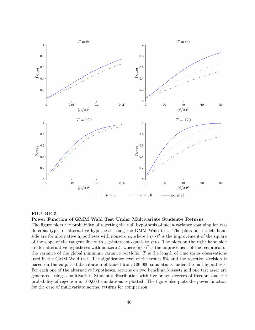
0 0.05 0.1 0.150

0.2

0.4

0.6

0.8

1

Pow

er

(α/σ)2

T = 60

0 20 40 60 800

0.2

0.4

0.6

0.8

1

Pow

er

(δ/σ)2

T = 60

0 0.05 0.1 0.150

0.2

0.4

0.6

0.8

1

Pow

er

(α/σ)2

T = 120

0 20 40 60 800

0.2

0.4

0.6

0.8

1

Pow

er

(δ/σ)2

T = 120

· – · – ν = 5 · · · · · · ν = 10 —— normal

FIGURE 5Power Function of GMM Wald Test Under Multivariate Student-t ReturnsThe figure plots the probability of rejecting the null hypothesis of mean-variance spanning for twodifferent types of alternative hypotheses using the GMM Wald test. The plots on the left handside are for alternative hypotheses with nonzero α, where (α/σ)2 is the improvement of the squareof the slope of the tangent line with a y-intercept equals to zero. The plots on the right hand sideare for alternative hypotheses with nonzero δ, where (δ/σ)2 is the improvement of the reciprocal ofthe variance of the global minimum variance portfolio. T is the length of time series observationsused in the GMM Wald test. The significance level of the test is 5% and the rejection decision isbased on the empirical distribution obtained from 100,000 simulations under the null hypothesis.For each one of the alternative hypotheses, returns on two benchmark assets and one test asset aregenerated using a multivariate Student-t distribution with five or ten degrees of freedom and theprobability of rejection in 100,000 simulations is plotted. The figure also plots the power functionfor the case of multivariate normal returns for comparison.

46

5 10 15 20 25 304

6

8

10

12

14

16

U.S. Bond

S&P 500

Australia

Canada

France

GermanyItaly

Japan

U.K.

Average

Return

Standard Deviation

FIGURE 6Average Return and Standard Deviation of U.S. and International InvestmentsThe figure plots the average return and sample standard deviation (in annualized percentage) ofS&P 500 index, 30-year U.S. Treasury bond, and seven international equity indices, computedusing monthly data over the period January 1970 to December 2007. The figure also plots theopportunity set from combining the S&P 500 index and the 30-year U.S. Treasury bond.

47

TABLE 1Sizes of Three Asymptotic Tests of Spanning Under Normality

The table presents the actual probabilities of rejection of three asymptotic tests of spanning (Wald (W ), like-lihood ratio (LR), and Lagrange multiplier (LM)), under the null hypothesis for different values of number ofbenchmark assets (K), test assets (N), and time series observations (T ). The asymptotic p-values of all threetests are set at 5% based on the asymptotic distribution of χ2

2N and the actual p-values reported in the tableare based on their finite sample distributions under normality assumption.

Actual Probabilities of Rejection

K N T W LR LM

2 2 60 0.078 0.063 0.048120 0.063 0.056 0.049240 0.056 0.053 0.050

10 60 0.249 0.125 0.037120 0.126 0.080 0.044240 0.082 0.063 0.047

25 60 0.879 0.500 0.015120 0.422 0.185 0.033240 0.183 0.099 0.042

5 2 60 0.094 0.076 0.059120 0.069 0.062 0.054240 0.059 0.056 0.052

10 60 0.315 0.172 0.058120 0.146 0.095 0.054240 0.089 0.069 0.052

25 60 0.932 0.638 0.038120 0.479 0.229 0.047240 0.203 0.113 0.049

10 2 60 0.126 0.105 0.084120 0.081 0.073 0.064240 0.064 0.060 0.057

10 60 0.446 0.279 0.118120 0.186 0.126 0.075240 0.103 0.081 0.061

25 60 0.981 0.838 0.146120 0.579 0.315 0.082240 0.238 0.138 0.063

48

TABLE 2Comparison of Power of Three Tests of Spanning Under Normality

The table presents the probabilities of rejection of Wald, likelihood ratio, and Lagrange multiplier tests ofspanning in 100,000 simulations under the alternative hypotheses when the number of test assets (N) is equalto 10 and the number of time series observations less the number of benchmark assets (T −K) is equal to 60.The size of the tests is set at 5% and the alternative hypotheses are summarized by two measures ω∗1 and ω∗2 ,where (T −K−1)ω∗1 and (T −K−1)ω∗2 are the eigenvalues of the noncentrality matrix THG−1. Numbers thatare boldfaced indicate the test has the highest power among the three tests.

Likelihood Ratio Test

ω∗2 = 0.0 ω∗2 = 0.3 ω∗2 = 0.6 ω∗2 = 0.9 ω∗2 = 1.2 ω∗2 = 1.5

ω∗1 = 0.0 0.0500

ω∗1 = 0.3 0.0823 0.1251

ω∗1 = 0.6 0.1226 0.1752 0.2338

ω∗1 = 0.9 0.1724 0.2307 0.2952 0.3612

ω∗1 = 1.2 0.2260 0.2913 0.3596 0.4257 0.4913

ω∗1 = 1.5 0.2834 0.3533 0.4228 0.4897 0.5533 0.6127

Wald Test

ω∗2 = 0.0 ω∗2 = 0.3 ω∗2 = 0.6 ω∗2 = 0.9 ω∗2 = 1.2 ω∗2 = 1.5

ω∗1 = 0.0 0.0500

ω∗1 = 0.3 0.0825 0.1243

ω∗1 = 0.6 0.1241 0.1735 0.2292

ω∗1 = 0.9 0.1739 0.2289 0.2901 0.3546

ω∗1 = 1.2 0.2299 0.2905 0.3547 0.4193 0.4834

ω∗1 = 1.5 0.2902 0.3538 0.4195 0.4829 0.5450 0.6042

Lagrange Multiplier Test

ω∗2 = 0.0 ω∗2 = 0.3 ω∗2 = 0.6 ω∗2 = 0.9 ω∗2 = 1.2 ω∗2 = 1.5

ω∗1 = 0.0 0.0500

ω∗1 = 0.3 0.0820 0.1260

ω∗1 = 0.6 0.1216 0.1754 0.2362

ω∗1 = 0.9 0.1685 0.2314 0.2981 0.3650

ω∗1 = 1.2 0.2199 0.2902 0.3617 0.4296 0.4962

ω∗1 = 1.5 0.2731 0.3496 0.4234 0.4930 0.5589 0.6195

49

TABLE 3Power of Step-Down Test of Spanning Under Normality

The table presents the probabilities of rejection of step-down test for two different alternatives, conditional onthe frontier of two benchmark assets is given in Figure 3. The first alternative (∆a = 0.0299) is a test assetthat doubles the slope of the asymptote to the efficient hyperbola of the two benchmark assets. The secondalternative (∆c = 67.16) is a test asset that reduces the standard deviation of the global minimum-varianceportfolio of the two benchmark assets from 4.8%/month to 4.5%/month. The step-down test is a sequential test.The first test is an F -test on α = 0N and the second test is an F -test of δ = 0N conditional on the restriction ofα = 0N . The null hypothesis of spanning is only accepted if we accept both tests. α1 and α2 are the significancelevels for the first and the second F -test, respectively. The number of time series observations is 62.

Probability of Rejection

Significance Levels ∆a = 0.0299 ∆a,∆b = 0

α1 α2 ∆b,∆c = 0 ∆c = 67.16

0.00000 0.05000 0.05117 0.874570.02532 0.02532 0.19930 0.809140.04040 0.01000 0.23996 0.702560.04905 0.00100 0.25889 0.422300.04914 0.00090 0.25908 0.410710.04924 0.00080 0.25927 0.397980.04933 0.00070 0.25946 0.383850.04943 0.00060 0.25966 0.367940.04952 0.00050 0.25985 0.349710.04962 0.00040 0.26004 0.328290.04971 0.00030 0.26023 0.302170.04981 0.00020 0.26041 0.268230.04990 0.00010 0.26060 0.218000.04995 0.00005 0.26070 0.177100.04996 0.00004 0.26071 0.165780.04997 0.00003 0.26073 0.152400.04998 0.00002 0.26075 0.135740.04999 0.00001 0.26077 0.112540.05000 0.00000 0.26068 0.05000

50

TABLE 4Sizes of Small Sample Tests of Spanning Under Nonnormality of Residuals

The table presents the probabilities of rejection of Wald (W ), likelihood ratio (LR), and Lagrange multiplier(LM) tests of spanning under the null hypothesis when the residuals follow a multivariate Student-t distributionwith five degrees of freedom. The rejection decision is based on 95th percentile of their exact distributions undernormality and the results for different values of the number of benchmark assets (K), test assets (N), and timeseries observations (T ) are based on 100,000 simulations.

Actual Probabilities of Rejection

K N T W LR LM

2 2 60 0.048 0.048 0.048120 0.049 0.050 0.050240 0.051 0.051 0.051

10 60 0.047 0.047 0.047120 0.046 0.046 0.046240 0.047 0.049 0.050

25 60 0.046 0.047 0.047120 0.046 0.046 0.046240 0.047 0.048 0.048

5 2 60 0.049 0.048 0.048120 0.051 0.051 0.051240 0.051 0.051 0.051

10 60 0.047 0.047 0.047120 0.048 0.048 0.048240 0.049 0.049 0.048

25 60 0.046 0.046 0.047120 0.046 0.046 0.046240 0.048 0.048 0.048

10 2 60 0.050 0.049 0.049120 0.049 0.049 0.049240 0.051 0.051 0.051

10 60 0.048 0.048 0.048120 0.049 0.049 0.049240 0.049 0.049 0.049

25 60 0.048 0.048 0.048120 0.047 0.047 0.047240 0.047 0.047 0.047

51

TABLE 5Sizes of Spanning Tests Under Multivariate Student-t Returns

The table presents the probabilities of rejection of using regular Wald test (W ) and two GMM Wald tests (Wa

and W ea ) of spanning under the null hypothesis when the returns follow a multivariate Student-t distribution

with five and with ten degrees of freedom. The number of benchmark assets is two and they are chosen tohave the same characteristics as the value-weighted and equally weighted market portfolios of the NYSE. Therejection decisions of the Wald tests are based on 95th percentile of χ2

2N . The table also presents the averageratios of the regular Wald tests to the GMM Wald tests. Results for different values of number of test assets(N) and time series observations (T ) are based on 100,000 simulations.

Actual Probabilities of Rejection Average Average

N T W Wa W ea W/Wa W/W e

a

Degrees of Freedom = 5

2 60 0.195 0.166 0.091 1.141 1.474120 0.197 0.113 0.078 1.305 1.564240 0.204 0.084 0.070 1.452 1.648

10 60 0.555 0.832 0.231 0.685 1.424120 0.469 0.536 0.112 0.962 1.519240 0.459 0.309 0.073 1.191 1.609

25 60 0.979 1.000 0.844 0.138 1.386120 0.851 0.995 0.346 0.569 1.480240 0.756 0.870 0.137 0.892 1.570

Degrees of Freedom = 10

2 60 0.116 0.134 0.090 1.003 1.136120 0.101 0.090 0.071 1.070 1.148240 0.095 0.070 0.063 1.113 1.156

10 60 0.373 0.747 0.243 0.677 1.142120 0.239 0.399 0.121 0.878 1.155240 0.183 0.201 0.079 0.998 1.162

25 60 0.942 1.000 0.871 0.157 1.136120 0.636 0.982 0.402 0.583 1.151240 0.406 0.724 0.172 0.826 1.160

52

TABLE 6Mean-Variance Spanning Tests on Seven International Equity Indices Under

NormalityThe table presents two sets of mean-variance spanning tests on seven international equity indices, using the S&P500 index and the 30-year U.S. Treasury bond as benchmark assets. The first test is an F -test of H0 : α = 0N

and δ = 0N . The second test is a step down test where F1 is an F -test of α = 0N , and F2 is an F -test of δ = 0N

conditional on α = 0N . The two tests are performed on each international equity index as well as jointly onall seven international equity indices. The reported p-values are exact under the normality assumption on theresiduals. The results are presented for the entire sample period as well as for its two subperiods.

Step-Down Test

Country α δ F -test p-value F1 p-value F2 p-value

Entire Period: 1970/1—2007/12

Australia 0.00597 0.468 14.479 0.000 4.734 0.030 24.026 0.000

Canada 0.00130 0.116 2.132 0.120 0.549 0.459 3.718 0.054

France 0.00492 0.305 6.700 0.001 3.361 0.067 9.987 0.002

Germany 0.00349 0.439 17.083 0.000 2.222 0.137 31.858 0.000

Italy 0.00416 0.536 12.999 0.000 1.610 0.205 24.355 0.000

Japan 0.00619 0.561 18.376 0.000 4.560 0.033 31.943 0.000

U.K. 0.00461 0.244 4.534 0.011 2.973 0.085 6.070 0.014

All 5.161 0.000 1.262 0.267 9.314 0.000

First Subperiod: 1970/1—1988/12

Australia 0.00668 0.545 9.113 0.000 2.174 0.142 15.970 0.000

Canada 0.00128 0.113 1.206 0.301 0.245 0.621 2.174 0.142

France 0.00639 0.320 3.389 0.035 1.939 0.165 4.819 0.029

Germany 0.00362 0.511 14.798 0.000 1.199 0.275 28.372 0.000

Italy 0.00468 0.595 8.420 0.000 0.839 0.361 16.011 0.000

Japan 0.01555 0.580 19.600 0.000 17.449 0.000 20.275 0.000

U.K. 0.00658 0.220 1.831 0.163 1.877 0.172 1.778 0.184

All 4.575 0.000 2.580 0.014 6.718 0.000

Second Subperiod: 1989/1—2007/12

Australia 0.00455 0.329 4.273 0.015 2.215 0.138 6.297 0.013

Canada 0.00136 0.120 0.879 0.417 0.314 0.576 1.448 0.230

France 0.00332 0.271 3.504 0.032 1.459 0.228 5.538 0.019

Germany 0.00284 0.299 3.106 0.047 0.788 0.376 5.429 0.021

Italy 0.00319 0.420 3.745 0.025 0.607 0.437 6.894 0.009

Japan −0.00343 0.508 6.527 0.002 0.602 0.439 12.473 0.001

U.K. 0.00280 0.285 5.463 0.005 1.480 0.225 9.426 0.002

All 1.738 0.046 0.795 0.593 2.722 0.010

53

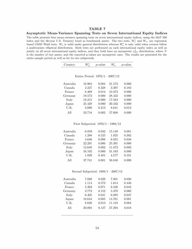
TABLE 7Asymptotic Mean-Variance Spanning Tests on Seven International Equity IndicesThe table presents four mean-variance spanning tests on seven international equity indices, using the S&P 500index and the 30-year U.S. Treasury bond as benchmark assets. The two tests, W e

a and Wa, are regressionbased GMM Wald tests. Wa is valid under general distribution whereas W e

a is only valid when returns followa multivariate elliptical distribution. Both tests are performed on each international equity index as well asjointly on all seven international equity indices, and they both have an asymptotic χ2

2N distribution, where Nis the number of test assets, and the reported p-values are asymptotic ones. The results are presented for theentire sample period as well as for its two subperiods.

Country W ea p-value Wa p-value

Entire Period: 1970/1—2007/12

Australia 10.964 0.004 21.573 0.000

Canada 2.227 0.328 3.397 0.183

France 8.469 0.014 10.373 0.006

Germany 19.573 0.000 28.422 0.000

Italy 18.215 0.000 17.584 0.000

Japan 25.428 0.000 30.432 0.000

U.K. 3.090 0.213 8.641 0.013

All 33.718 0.002 57.608 0.000

First Subperiod: 1970/1—1988/12

Australia 6.859 0.032 15.149 0.001

Canada 1.288 0.525 1.925 0.382

France 4.646 0.098 6.055 0.048

Germany 22.291 0.000 25.391 0.000

Italy 12.648 0.002 11.872 0.003

Japan 34.102 0.000 31.163 0.000

U.K. 1.829 0.401 4.577 0.101

All 37.741 0.001 56.848 0.000

Second Subperiod: 1989/1—2007/12

Australia 7.080 0.029 7.801 0.020

Canada 1.114 0.573 1.614 0.446

France 5.303 0.071 6.320 0.042

Germany 3.773 0.152 5.378 0.068

Italy 6.405 0.041 6.095 0.047

Japan 10.644 0.005 14.761 0.001

U.K. 8.620 0.013 11.124 0.004

All 20.094 0.127 27.294 0.018

54