An Empirical Comparison of Methods for Temporal

Distribution and Interpolation at the National Accounts

Baoline Chen

Office of Directors

Bureau of Economic Analysis 1441 L St., NW, Washington, DC 20230

Email: Baoline.chen@bea.gov

August 30, 2007

Abstract

This study evaluates five mathematical and five statistical methods for temporal disaggregation in an attempt to select the most suitable method(s) for routine compilation of sub-annual estimates through temporal distribution and interpolation in the national accounts at BEA. The evaluation is conducted using 60 series of annual data from the National Economic Accounts, and the final sub-annual estimates are evaluated according to specific criteria to ensure high quality final estimates that are in compliance with operational policy at the national accounts. The study covers the cases of temporal disaggregation when 1) both annual and sub-annual information is available; 2) only annual data are available; 3) sub-annual estimates have both temporal and contemporaneous constraints; and 4) annual data contain negative values. The estimation results show that the modified Denton proportional first difference method outperforms the other methods, though the Casey-Trager growth preservation model is a close competitor in certain cases. Lagrange polynomial interpolation procedure is inferior to all other methods. _________ I would like to express our great appreciation to Pierre Cholette from Statistics Canada, David Findley and Brian Monsell from the Census Bureau, Roberto Barcellan from Eurostats, and Nils Maehle from the MIF for providing us the software programs and related documentations used in the estimation experiment and for their helpful discussions on the subject. I am also very grateful to Stephen Morris and Aaron Elrod for the tremendous amount of estimation work and tedious statistical analysis they have helped with on the project. Thanks go to Brent Moulton, Marshall Reinsdorf and Ana Aizcorbe for their helpful comments.

1

1. Introduction

National accounts face the task of deriving a large number

of monthly or quarterly estimates using mostly annual data and

some less reliable or less comprehensive quarterly or monthly

information from proxy variables known as indicators. The annual

data are usually detailed and of high precision but not very

timely; they provide the most reliable information on the overall

level and long-term movements in the series. The quarterly or

monthly indicators are less detailed and of lower precision but

they are timely; they provide the only explicit information about

the short-term movements in the series. Statistically speaking,

the process of deriving high frequency data from low frequency

data and, if it is available, related high frequency information

can be described as temporal disaggregation. To simplify the

exposition, we follow the terminology used in the literature to

refer to the low frequency data as annual data and the high

frequency data as sub-annual data (Cholette and Dagum, 2006).

Typically the annual sums of the sub-annual indicator

series are not consistent with the annual values, which are

regarded as temporal aggregation constraints or benchmarks, and

quite often the annual and sub-annual series exhibit inconsistent

annual movements. The primary objective of temporal

disaggregation is to obtain sub-annual estimates that preserve as

much as possible the short-term movements in the indicator series

under the restriction provided by the annual data which exhibit

long term movements of the series. Temporal disaggregation

combines the relative strength of the less frequent annual data

and the more frequent sub-annual information.

Temporal disaggregation also covers the cases where sub-

annual information is not available. In addition, it covers the

cases where a set of sub-annual series are linked by some

accounting relationship regarded as a contemporaneous aggregation

constraint. In such cases, temporal disaggregation should

2

produce sub-annual estimates that are consistent with both

temporal and contemporaneous aggregation constraints.

Temporal disaggregation is closely related to but different

from benchmarking. They are related in that benchmarking or

temporal disaggregation arises because of the need to remove

discrepancies between annual benchmarks and corresponding sums of

the sub-annual values. They are different because the

benchmarking problem arises when time series data for the same

target variable are measured at different frequencies with

different level of accuracy, whereas temporal disaggregation

deals with the problem where the sub-annual data are not for the

same target variable as the annual data.

There are two facets of the temporal disaggregation

problem: temporal distribution and interpolation. Temporal

distribution is needed when annual data are either the sum or

averages of sub-annual data. In general distribution deals with

all flow and all index variables. Interpolation, on the other

hand, deals with estimation of missing values of a stock

variable, which at points in time have been systematically

skipped by the observation process. In the estimation of

quarterly variables, interpolation is used for all stock

variables whose annual values equal those of the fourth (or the

first) quarter of the same year. An example is population at the

end of a year which equals the population at the end of the

fourth quarter of the same year. Sometimes sub-annual estimates

need to be made before the relevant annual and/or quarterly

information is available. In such cases temporal distribution

and interpolation are combined with extrapolation to produce sub-

annual estimates.

There is a wide variety of methods for temporal

distribution, interpolation and extrapolation. Because

benchmarking and temporal disaggregation deal with similar

statistical problems, the methods used for temporal

disaggregation are very similar to those used for benchmarking.

To a large extent, the choice of methods depends on two factors:

3

basic information available for estimation, and preference or

operational criteria suitable for either a mathematical approach.

There are three general cases regarding the availability of

information: 1) information is available on both an annual and

sub-annual basis; 2) information is only available on an annual

basis; and 3) annual and/or sub-annual information is not yet

available at the time of estimation.

If both annual and sub-annual information is available, the

choices are pure numerical procedures, mathematical benchmarking

methods, or statistical methods. Examples of pure numerical

procedures are linear interpolation or distribution procedures,

and Lagrange interpolation procedure. The most widely used

mathematical benchmarking methods are the Denton adjustment

method (Denton, 1971) and its variants (Helfand et al, 1977;

Cholette, 1979) and the Causey-Trager method (Causey and Trager,

1981; Bozik and Otto, 1988). The most commonly used statistical

methods are the Chow-Lin regression methods (1971) and their

extensions (Bournay and Laroque, 1979; Fernandez, 1981;

Litterman, 1983); time-series ARIMA models (Hillmer and Trabelsi,

1987); and generalized regression-based methods (Cholette and

Dagum, 2006). More recently, time series models such as

benchmarking based on signal extraction (Durbin and Quenneville,

1997; Chen, Cholette and Dagum, 1997) and the structural time

series models in state space representation for interpolation and

temporal distribution (Harvey and Pierse, 1984; Gudmundson, 1999;

Proietti, 1999; and Aadland, 2000) have also been developed.

If, on the other hand, only annual data are available,

choices are mathematical, numerical smoothing methods, and time

series ARIMA models. Commonly used smoothing methods are those

developed by Boot, Feibes, and Lisman (1970), and by Denton

(1971). A commonly used numerical smoothing procedure is the

cubic spline. The ARIMA models developed to generate sub-annual

estimates in the absence of sub-annual information are those by

Stram and Wei (1986) and Wei and Stram (1990).

4

When annual and/or sub-annual information for the current

year is not yet available at the time of estimation,

extrapolation is necessary. If only sub-annual indicator values

are available, they can be used to extrapolate the annual

aggregate, which can then be used to distribute or interpolate

the sub-annual estimates. The idea is that the indicator and the

annual series have the same time profile and, thus, they have the

same growth rate. However, if no information on the indicator is

yet available, the sub-annual estimates for the current periods

can only be derived from the extrapolation of previous sub-annual

estimates or from interpolation of the extrapolated annual data.

If the available information is not sufficiently reliable and/or

not complete, it is then necessary to consider some classical

extrapolation methods based on previously available sub-annual

information or based on the methods that use related series.

Like most government statistical agencies, deriving sub-

annual estimates using only annual data and incomplete sub-annual

information is a routine practice in the national accounts at

BEA. The national accounts at BEA have experimented with a

variety of techniques over the years. Up to the 1970s, the

Bassie adjustment procedure (Bassie, 1958) was the major method

used at BEA. Bassie was the first to develop a method for

constructing sub-annual series whose short-term movements would

closely reflect those of a related (indicator) series while

maintaining consistency with annual aggregates. The Bassie

procedure tends to smooth the series, and hence, it can seriously

disturb the period-to-period rates of change in sub-annual series

that exhibit strong short-term variation. Because the Bassie

method operates on only two consecutive years of data, using the

Bassie method often results in a step problem if data of several

years are adjusted simultaneously. Moreover, the Bassie method

does not support extrapolation.

Because of the unsatisfactory results from the Bassie

procedure, the Minimum Constrained Variance Internal Moving

Average (MCVIM) procedure was introduced to the national accounts

5

during the 1980s, and both Bassie and MCVIM were used for

interpolation and temporal distribution. MCVIM method is based

on the idea of deriving sub-annual estimates by minimizing the

variance in the period-to-period changes in the estimated sub-

annual series. However, in the 1990s, the Bassie and MCVIM

procedures were largely replaced by a purely numerical procedure

known as the Lagrange polynomial interpolation procedure when BEA

transferred to the AREMOS time-series database.

Polynomial interpolation is a method that takes a

collection of n points of annual data and constructs a polynomial

function of degree n-1 that passes these annual values. Using

the Lagrange polynomial interpolation procedure assumes that the

polynomial function that passes the annual values is a Lagrange

polynomial; the n points of annual values are called Lagrange

data. In general, Lagrange polynomial interpolation can be

considered if only the approximation of level is needed.

Lagrange polynomial interpolation procedure has some serious

known drawbacks. First of all, Lagrange polynomial interpolation

is a global method, and hence, it requires some information about

the function globally. In practice, the approximated values

based on a certain assumed degree of polynomial could sharply

disagree with the actual values of the function due to lack of

information about the function globally. Secondly, the

approximation error may be unbounded as the degree of polynomial

increases. Thirdly, computation of the Lagrange is costly,

because it requires a large number of evaluations. The Lagrange

polynomial interpolation formula uses 3n additions, 2n divisions

and 2n multiplications even when done most efficiently.

Lagrange polynomial interpolation has not proven

satisfactory in the national accounts. The major problems

encountered are inconsistency in the short-term movements shown

in the indicator and final estimated sub-annual series, the sharp

increase or decrease at the end of the interpolated series, and

the jumpy links between the newly interpolated span of a series

and the previously benchmarked span of the series. An added

6

difficulty arises in practice because Lagrange polynomial

interpolation in AREMOS uses five annual data points, but under

the current revision policy at the national accounts, only data

of the most recent three years can be used in estimation. Thus,

it requires a forward extrapolation of two annual data points

before Lagrange polynomial interpolation can be performed.

Although there is a recommended extrapolation procedure, analysts

often have to make judgmental decisions on the extrapolation

procedure to be used when encountering various data problems.

Sub-annual estimates generated from the Lagrange polynomial

interpolation procedure in AREMOS are directly affected by the

choices of extrapolation procedures.

Because of the difficulties experienced using Lagrange

polynomial interpolation, alternative methods such as linear

interpolation, Bassie and MCVIM methods continue to be used in

various parts of the national accounts. To improve the quality

of sub-annual estimates in the national accounts, there is strong

interest in finding an appropriate standardized method for

temporal disaggregation at the national accounts. Various

attempts have been made in recent years by researchers at BEA in

a search for a better method for temporal disaggregation (Klick,

2000; Loebach 2002).

The objective of this study is to evaluate a number of

existing mathematical and statistical methods for temporal

disaggregation based on certain specific criteria and to

recommend the most suitable method(s) for practice in the

national accounts. The evaluation is conducted using 60 annual

data series from the National Economic Accounts. The study will

cover the cases where 1) both annual and indicator series are

available; 2) only annual data are available; 3) annual series

contain both positive and negative values; and 4) annual series

have both temporal and contemporaneous constraints. To evaluate

different methods for temporal disaggregation, three software

packages were used: ECOTRIM from Eurostats, BENCH from the

Statistics of Canada, and BMARK from the U.S. Census Bureau.

7

Each software package offers some unique features and has

advantages over the others in certain aspects of computation.

The plan for the rest of the paper is as follows. Section

2 presents various mathematical and statistical methods for

temporal disaggregation. Section 3 discusses the five criteria

for evaluation. Section 4 presents and discusses the estimation

results. Section 5 evaluates the methods and software package

used in the experiment and suggests method(s) and software for

temporal disaggregation at the national accounts. Section 6

concludes the paper.

2. Methods for Temporal Disaggregation

There is a variety of mathematical and statistical methods

developed for temporal disaggregation. The distinction between a

mathematical and a statistical method is that a mathematical

model treats the process of an unknown sub-annual series as

deterministic and treats the annual constraints as binding,

whereas a statistical model treats the process of an unknown sub-

annual series as stochastic and allows the annual constraints to

be either binding or not binding. The choice of a particular

method depends to a large extend on the information available for

estimation and subjective preference or operational criteria.

Because the objective of this study is to search for the

most suitable method(s) for interpolation and temporal

distribution for routine compilation of sub-annual estimates in

the national accounts, we focus on three mathematical methods:

the Denton adjustment method (1971) and its variants; the Causey-

Trager growth preservation method (Causey and Trager, 1981); and

the smoothing method (Boot, Feibes and Lisman, 1970). We shall

also review five extensions of the Chow-Lin regression method

(Chow and Lin, 1971), which include an AR(1) model estimated by

applying maximum likelihood (ML) and generalized least squares

(GLS), the Fernandez random walk model (1981), and the Litterman

random walk-Markov model (1998) estimated by applying ML and GLS.

8

In this section we shall briefly describe the mathematical

and statistical methods being reviewed in this study and discuss

the advantages and disadvantages of these methods.

2.1 Mathematical Methods for Temporal Disaggregation

We shall start with the original Denton adjustment method

(Denton, 1971) and its variants, and then describe the Causey-

Trager method (Causey and Trager, 1981). These methods are

suitable for interpolation or distribution when both annual and

sub-annual indicator values are available. We shall then discuss

the Boot, Feibes and Lisman smoothing method for distribution and

interpolation when only annual values are available.

To formalize our discussion, we first define some notation.

Let zt and xt denote the sub-annual indicator series and sub-

annual estimates from distribution or interpolation for sub-

annual period t = 1, 2 …, T, where T is the total number of sub-

annual periods in the sample. Let ym denote the annual value of

year m for m = 1, 2 …, M, where M is the total number of annual

values in the sample. Let kmt denote the coverage fraction of

sub-annual estimate of period t, e.g. for quarterly or monthly

series of index variables, kmt = 1/4 or kmt = 1/12; for flow

variables, kmt = 1. Also let t1m and t2m denote the first and last

periods covered by the m-th annual value, e.g. if m = 2, for a

quarterly series, t = t1m = 5 and t = t2m = 8 respectively. Let ∆

denote backward first difference operator, e.g., ∆xt = xt – xt-1,

∆zt = zt – zt-1, ∆xt - ∆zt = ∆(xt – zt) = (xt – zt) – (xt-1 – zt-1).

Let ∆2 denote the backward second difference operator, e.g., ∆2xt

- ∆2zt = ∆2(xt – zt) = ∆(xt – zt) – ∆(xt-1 – zt-1).

2.1.1 The original Denton adjustment method and its variants

The original Denton adjustment method is based on the

principle of movement preservation. According to this principle,

9

the sub-annual series xt should preserve the movement in the

indicator series, because the movement in the indicator series is

the only information available. Formally, we specify a penalty

function, P(x, z), where x = (x1 …, xT)’ and z = (z1 …, zT)’ are

Tx1 column vectors of final sub-annual and indicator values. The

mathematical problem of the original Denton adjustment model is

to choose final sub-annual estimates, x, so as to minimize the

penalty function P(x, z), subject to the temporal aggregation

constraints,

ym = ∑=

m

m

t

tttmtxk

2

1

,

for m = 1, 2 …, M, in the cases of distribution of index or flow

variables. In the cases of interpolation of stock variables, the

constraint becomes

ym = mtx 1, or ym =

mtx 2,

for m = 1, 2 …, M, with either the first or the last sub-annual

estimate equals the annual value for year m.

Let y = (y1 …, yM)’ be a column vector of M annual values;

let B be a TxM matrix that maps sub-annual estimates to annual

constraints; and let A be a TxT weighting matrix. Then, the

original Denton model can be specified in the matrix form as

(1) Minx P(x, z) = )zx(A)'zx( −− ,

Subject to

(2) y = B’x.

The solution to the final sub-annual estimate is

10

(3) x = z + C(y – B’z),

where y – B’z measures the annual discrepancy and C represents

the distribution rule determining how the annual discrepancy is

distributed to each sub-annual period. If A is ITxT, then C will

be the inverse of the number of sub-annual periods in a year.

The annual discrepancy would then be distributed evenly to each

sub-annual period. Apparently, that is not a good choice of

distribution rule.

Denton proposed several variants of the original movement

preservation model based on the first or higher order difference

of the final sub-annual estimates and the indicator series. The

most widely used are the additive and proportional first and

second difference variants.

1) The additive first difference variant preserves the sample

period-to-period change in the level of the final sub-annual

estimates and the indicator values, (xt – zt), under the annual

constraint. As a result, xt tends to be parallel to zt. The

objective in this case is achieved by minimizing the sum of

squares of ∆(xt – zt), so the penalty function is P(x, z) =

∑ −∆=

T

ttt )]zx([

1

2 .

2) The proportional first difference variant preserves the

proportional period-to-period change in the final sub-annual

estimates and the indicator series, xt/zt. As a result, xt tends

to have the same period-to-period growth rate as zt. The

objective here is achieved by minimizing the sum of squares of

∆(xt/zt) = (xt/zt) – (xt-1/zt-1), and the penalty function in this

case is P(x, z) = ∑ −= −

−T

t t

t

t

t )z

x

z

x(1

2

1

1 .

11

3) The additive second difference variant preserves the sample

period-to-period change in ∆(xt – zt) as linear as possible. In

this case, the objective is to minimize the sum of squares of

∆2(xt – zt), and the penalty function is P(x, z) = ∑ −∆=

T

ttt )]zx([

1

22 .

4) The proportional second difference variant preserves the

sample period-to-period change in ∆(xt/zt) as linear as possible.

The objective in this case is to minimize the sum of squares of

∆2(t

t

zx

), and the penalty function is P(x, z) = ∑ −∆= −

−T

t t

t

t

t )]z

x

z

x([

1

2

1

1 .

Denton imposed the initial conditions that no adjustments

are to be made in the indicator values outside of the sample.

Thus, in the first difference variants, the initial condition

boils down to x0 = z0, and in the second difference variants, the

initial conditions boil down to xo = zo and x-1 = z-1. Such

initial conditions result in a major short-coming of the original

Denton method, because it induces a transient movement at the

beginning of the series. It forces the final sub-annual

estimates to equal the original series at time zero and results

in the minimization of the first change (x1 – z1). Such transient

movement defeats the principle of movement preservation. Helfand

et al. (1977) solved this problem by modifying the penalty

function to P(x, z) = ∑ −∆=

T

ttt )]zx([

2

2 for the additive first

difference variant, and P(x, z) = ∑ ∆=

T

t t

t)z

x(2

2 for the proportional

first difference variant. The modified first difference variants precisely omit this first term to solve this short-coming of the

original Denton method. The penalty functions for the second

difference variants are modified accordingly.

12

2.1.2 The Causey-Trager growth preservation model

The growth preservation model is first developed by Causey

and Trager (1981) and later revised by Trager (1982). They

propose that instead of preserving the proportional period-to-

period change in final sub-annual estimates and indicator series

xt/zt, the objective should be to preserve the period-to-period

percentage change in the indicator series. As a result, the

period-to-period percentage change in xt tends to be very close

to that in zt. This objective is achieved by minimizing the sum

of squares of (xt/xt-1 – zt/zt-1). Formally, the mathematical

problem of the Causey-Trager model is

(4) Minx P(x, z) = ∑ −= −−

T

t t

t

t

t ]zz

xx

[2

2

11,

subject to (2), the same temporal constraints as those specified

in the original Denton model.

The Causey-Trager model is non-linear in the final sub-

annual estimates xt, and thus, it does not have a closed form

solution. The Causey-Trager model is solved iteratively using

the solution to the Denton proportional first difference model as

the starting values. Causey (1981) provided a numerical

algorithm using steepest descent to obtain the final sub-annual

estimates xt, t = 1, 2 …, T. This numerical algorithm was later

revised by Trager (1982). Because the Causey-Trager model is

non-linear and is solved iteratively, the computational cost is

higher compared to the Denton proportional first difference

model, which has a closed form solution.

2.1.3. The Boot, Feibes and Lisman smoothing method (BFL)

Smoothing methods are suitable for univariate temporal

disaggregation when only annual data are available. The basic

13

assumption of smoothing methods is that the unknown sub-annual

trend can be conveniently described by a mathematical function of

time. Because no sub-annual information is available, the sub-

annual path is given a priori or chosen within a larger class,

such as that the necessary condition of satisfying temporal

aggregation constraints and the desirable condition of smoothness

are both met. One such smoothing method is the BFL method.

There are two versions of the BFL method, the first difference

model and the second difference model.

The objective of the first difference model is to minimize

period-to-period change in the level of final sub-annual

estimates ∆xt subject to the annual constraints. Formally, the

problem is to

(5) Minx P(x) = ∑ −=

−

T

ttt )xx(

2

21 ,

subject to (2). The constraints are the same as those specified

in the original Denton model.

The objective of the second difference model is to keep the

period-to-period change in ∆xt as linear as possible. This

objective is achieved by minimizing the sum of squares of ∆2xt =

(∆xt - ∆xt-1) subject to annual constraints. Formally, the second

difference model is

(6) Minx P(x) = ∑ −∆=

−

T

ttt )]xx([

2

21 ,

subject to (2).

Like other smoothing methods, the BFL method does not allow

extrapolation of sub-annual estimates, because it is designed

only to give a sub-annual breakdown of the available annual data.

Thus, to produce the current year estimates, a forecast value of

14

the current year annual value is needed. All sub-annual periods

of the current year are then estimated at the same time.

2.2 Regression Methods

There have been quite a number of statistical methods

developed for temporal disaggregation. These methods are

designed to improve upon the mathematical methods discussed

above, which do not take into consideration certain behaviors of

economic time series data. Some examples of the statistical

benchmarking methods are optimal regression models (Chow and Lin,

1971; Bournay and Laroque; 1979; Fernandez, 1983; Litterman,

1983), dynamic regression models (De Fonzo, 2002), unobserved

component models or structural time series models using Kalman

filter to solve for optimal estimates of the missing sub-annual

observations (Gudmundson, 1999; Hotta and Vasconcellos, 1999;

Proietti, 1999; Gomez, 2000), and Cholette-Dagum regression-based

benchmarking methods (Cholette and Dagum, 1994, 2006).

For our purpose, we will limit our discussion on the more

widely used Chow-Lin regression model and its variants, which are

used in our experiment. We shall also briefly discuss the

Cholette-Dagum regression-based method, because, in some respect,

it can be considered a generalization of the Denton benchmarking

approach. The structural time series models formulated in state

space representation for interpolation and temporal distribution

are not yet fully corroborated by empirical applications, and,

therefore, will not be discussed here.

2.2.1 The Chow-Lin regression method

Chow-Lin (1971) developed a static multivariate regression

based method for temporal disaggregation. They argue that sub-

annual series to be estimated could be related to multiple

series, and the relationship between the sub-annual series and

the observed related sub-annual series is

15

(7) xt = ztβ + ut,

where x is a Tx1 vector, z is a Txp matrix of p related series, β

is px1 vector of coefficients, ut is a Tx1 vector of random

variables with mean zero and TxT covariance matrix V. They

further assume that there is no serial correlation in the

residuals of the sub-annual estimates.

In matrix form, the relationship between annual and sub-

annual series can be expressed as

(8) y = B’x = B’zβ + B’u.

Chow-Lin derives the solutions by means of the minimum

variance linear unbiased estimator approach. The estimated

coefficient β) is the GLS estimator with y being the dependent

variable and annual sums of the related sub-annual series as the

independent variables. The estimated coefficients are

(9) β)

= [z’B(B’VB)-1B’z]-1z’B(B’VB)-1y,

and the linear unbiased estimator of x is

(10) x) = zβ) + VB(B’VB)-1[y – B’zβ

)].

The first term in (10) applies β) to the observed related

sub-annual series of the explanatory variables. The second term

is an estimate of the Tx1 vector u of residuals obtained by

distributing the annual residuals y – B’zβ) with the TxM matrix

VB(B’VB)-1. This implies that if the sub-annual residuals are

serially uncorrelated, each with variance σ2, then V = σ2ITxT, and

16

then annual discrepancies are distributed in exactly the same

fashion as Denton’s basic model with A = ITxT.

The assumption of no serial correlation in the residuals of

sub-annual estimates is generally not supported by empirical

evidence. Chow-Lin proposes a method to estimate the covariance

matrix V under the assumption that the errors follow a first-

order autoregressive AR(1) process. There are two static

variants of the Chow-Lin approach intended to correct the serial

correlation in the sub-annual estimates. One is the random walk

model developed by Fernandez (1981), and the other is the random

walk-Markov model developed by Litterman (1983).

2.2.2 The Random walk model

Fernandez argues that economic time series data are often

composed of a trend and a cyclical component, and he proposes to

transform the series to eliminate the trend before estimation.

He sets up the relationship between the annual and the sub-annual

series as that in equation (8) and derives β) and the linear

unbiased estimator of x as those in equations (9) and (10).

However, Fernandez argues that the sub-annual residuals follow

the process

(11) ut = ut-1 + εt,

where εt ∼ N(0, VTxT), is a vector of random variables with mean

zero and covariance matrix VTxT. Based on this specification, the

relationship between x and z is

(12) xt – xt-1 = ztβ - zt-1β + ut – ut-1,

which can be expressed as

(13) Dxt = Dztβ + Dut,

17

where D is the first difference operator.

The relationship between the annual and sub-annual series

also needs to be transformed accordingly, because the sum of Dxt

is not equal to y. Fernandez shows such relationship in the

matrix form as

(14) ∆y = QDx = QDzβ + QDu,

where ∆ is similar to D but the dimension of ∆y is MxM, and Q is

MxT matrix. This specification holds if the final sub-annual

estimates x in year 0 are constant, an assumption considered

reasonable for large sample size.

Given the sub-annual residual process specified by

Fernandez and setting QD = B’, the solutions are

(15) x) = zβ) + (D’D)-1B(B’(D’D)-1 B)-1[y – B’zβ

)],

(16) β) = [z’B(B’(D’D)-1B)-1B’z]-1z’B(B’(D’D)-1B)-1y.

If A = D’D, these solutions are identical to those derived

from the first difference regression model. Fernandez concludes

that 1) before estimating the sub-annual series through

interpolation or distribution, the behavior of the series should

be studied. If the series is non-stationary and serially

correlated, then the first difference data should be used to

transform the data in order to obtain stationary and uncorrelated

series; 2) if the first difference is not enough, other

transformation is needed to convert residuals to serially

uncorrelated and stationary variables; and 3) given proper

transformation, the degree of serial correlation can be tested by

generalized least square estimation.

18

2.2.3 The Random walk-Markov model

Litterman (1983) argues that the relationship between

short-run movements in x and zβ is fairly stable in most cases,

but the levels of x and zβ may vary over time. He points out

that Chow-Lin’s specification of the covariance matrix, V =

Inxnσ2, is not adequate if the sub-annual residuals exhibit serial

correlation, because this specification would lead to step

discontinuity of the sub-annual estimates between the annual

periods as it allocates each annual residual among all sub-annual

estimates. He also argues that Chow-Lin’s treatment of serial

correlation is only adequate if the error process is stationary.

Litterman argues that Fernandez’ random walk assumption for

the sub-annual residual term could remove all serial correlation

in the annual residuals when the model is correct. However, in

some cases, Fernandez’ specification does not remove all serial

correlation. Litterman proposes the following generalization of

the Fernandez method,

(17) xt = ztβ + ut,

(18) ut = ut-1 + εt,

(19) εt = αεt-1 + et,

where et ∼ N(0, V), is a vector of random variables with mean

zero and covariance matrix V, and the implicit initial condition

is that u0 = 0. In fact, given the specification of his model,

Litterman’s model is considered an ARIMA (1, 1, 0) model.

Under this assumption of the sub-annual residual process,

Litterman transforms the annual residual vector into E = HDu and

derived the covariance matrix V as

19

(20) V = (D’H’HD)-1σ2,

where H is an TxT matrix with 1 in the diagonal elements and -α

in the entries below the diagonal elements. The solutions of x

and β are respectively

(21) x = z β + (D’H’HD)-1B’[B(D’H’HD)-1B’]-1[Y – B’z β],

(22) β = [z’B(B’(D’H’HD)-1B’)-1B’z]-1z’B(B’(D’H’HD)-1B’)-1Y.

Litterman suggests two steps to estimate β and derives the

linear unbiased estimator of x. The first step is to follow the

estimator derived by Fernandez and to generate the annual

residuals, U = B u . The second step is to estimate α by forming

the first-order autocorrelation coefficient of the first

difference of the annual residuals and solving for α. Therefore,

Litterman’s method also uses first difference data rather than

the level data.

2.2.4 AR(1) model

Apart from the random walk models, there are also attempts

to model the errors as an AR(1) process. Bournay and Laroque

(1979) propose that the sub-annual errors follow an AR(1) process

(11) ut = ρut-1 + εt,

where εt ∼ N(0, σ2) is white noise, and |ρ| < 1. The value of the

coefficient ρ represents the strength of movement preservation of

the distribution or interpolation model. Bournay and Laroque

suggested that ρ = .999, which represents very strong movement

preservation. The AR(1) model can be estimated by applying ML or

20

GLS. Cholette and Dagum (2006) suggest that ρ be set to .9 for

monthly series and to .93 for quarterly series.

Cholette and Dagum developed Regression-based benchmarking

method (1994), which consists of two basic models, the additive

model and the multiplicative model.

The Cholette-Dagum additive benchmarking model is

formulated as follows,

(12) zt = ∑ β=

H

hhthr

1+ xt + et, t = 1, …, T,

subject to

(13) ym = ∑=

m

m

t

tttmtxj

2

1

+ εt, m = 1, …, M,

where E(et) = 0, E(etet-1) = λ−

λσσ 1tt ωt, λ measures degree of

heteroscedasticity, E(εm) = 0 and E(εmet) = 0.

The first term in (12) specifies deterministic time

effects. If H = 1 and rth = -1, this term captures the average

level discrepancy between the annual and the sub-annual data. In

some cases, a second regressor is used to capture a deterministic

trend in the discrepancy. In some cases, rth may be absent, which

implies H = 0. The Cholette-Dagum model allows the annual

constraint to be not binding. This is the case if εt is nonzero.

The above additive model can be modified into proportional model.

One can see from (12) and (13) that by setting the parameters to

certain default values, the Cholette-Dagum additive model can be

modified to approximate the Denton additive and proportional

models.

The Cholette-Dagum multiplicative benchmarking model is

formulated as follows,

(14) lnzt = ∑ β=

H

hhth nr

1l + lnxt + lnet, t = 1, …, T,

21

subject to (13), where E(εm) = 0 and E(εmεm) = 2mεσ .

The multiplicative model requires that both annual and sub-annual

indicator observations to be positive in order to avoid negative final

estimates of sub-annual values. Typically, the deterministic regressor

is a constant, i.e. H = 1 and rHt = -1, which captures the average

proportional level difference between the annual and the sub-annual

indicator data. If this is the case, the first term in (13) is a

weighted average of the proportional annual discrepancies. Similar as

in the additive model, in some cases, a second regressor is used to

capture a deterministic trend in the proportional discrepancy, or the

regressor may be absent, in which case H = 0. By setting the

parameters in the multiplicative model to certain default values, the

multiplicative model can be modified to approximate the Causey-Trager

growth preservation model.

3. Test Criteria and Estimation Strategy

Our objective is to select a method or methods most

suitable for routine temporal distribution and interpolation in

the national accounts. The most suitable method(s) should

generate final sub-annual estimates that best satisfy certain

pre-specified criteria and should be easy to implement given the

operational criteria set by the national accounts.

3.1 Test Criteria

Five basic criteria should be used to evaluate the final

sub-annual estimates generated using different methods.

1) Temporal aggregation constraint must be satisfied. This means

that for each annual period, the sub-annual estimates must

aggregate or average to the annual benchmarks. The temporal

discrepancy can be measured with respect to the indicator series

or to the estimated final sub-annual series. Temporal

22

discrepancies with respect to indicator series show how much the

indicator series need to be adjusted so that the temporal

constraints can be satisfied, and could be large because the

indicator and the annual benchmark in general do not directly

measure the same target variable. Temporal discrepancies with

respect to the final sub-annual estimates measure how well the

temporal aggregation constraints are satisfied, and should be

null if the annual benchmarks are binding.

Temporal discrepancies can be measured algebraically (in

level) or proportionally. For year m = 1, 2 …, M, algebraic

temporal discrepancy with respect to final sub-annual estimates

is computed as

(3.1) AxD = ym - ∑

=

m

m

t

tttmtxk

2

1

, for indicator and flow variables,

or

AxD = ym – xt1m (or ym – xt2m), for stock variables.

Correspondingly, proportional temporal discrepancy with respect

to final sub-annual estimates is computed as

(3.2) PxD = ym/ ∑

=

m

m

t

tttmtxk

2

1

, for indicator and flow variables,

or

PxD = ym/xt1m (or ym/xt2m), for stock variables.

Algebraic and proportional discrepancies with respect to the

indicator series AzD and P

zD can be written out simply by

replacing xt with zt in (3.1) and (3.2).

Two statistics of temporal discrepancies are empirically

useful. The means of discrepancies measure the level or

proportional difference between the annual benchmarks and the

indicator series, or between the annual benchmarks and the

estimated sub-annual series, of all annual periods in the sample.

23

The standard deviation of discrepancies measures the dispersion

of discrepancies of all sample periods. A large standard

deviation may imply erratic discrepancies over sample periods,

suggesting a contradiction between the annual and indicator

variables, and it may also imply that in the process of

satisfying the annual benchmarks, temporal distribution or

interpolation distorts the movements of the indicator series.

Erratic discrepancies may suggest low reliability of the

indicator series.

2) Short-term movements in the indicator series should be

preserved as much as possible. Short-term movement preservation

can be measured in terms of level, proportion, and growth rates.

Different methods are designed to achieve different objectives of

short-term movement preservation. For example, the Denton

additive first difference method is designed to preserve period-

to-period movements in the indicator series. Thus, the objective

is to minimize period-to-period change between the sub-annual and

indicator series. The resulting sub-annual estimates tend to be

parallel to the indicator series. The Denton proportional first

difference method is designed to preserve proportional period-to-

period movements in the final sub-annual estimates and the

indicator series. Therefore, the objective is to minimize

period-to-period change in the ratio of the final sub-annual

estimates to the indicator series. Final sub-annual series

estimated using this method tends to have the same period-to-

period percentage changes as the indicator series. The Causey-

Trager method is designed to preserve period-to-period growth

rate in the indicator series. The resulting sub-annual estimates

and the indicator series tend to have the same growth rates.

Two statistics can be used to measure short-term movement

preservation: 1) the average absolute change in period-to-period

differences between the final sub-annual estimates and the

indicator series of all sub-annual periods in the sample, cL; and

2) the average absolute change in period-to-period growth rates

24

between the final sub-annual estimates and the indicator series

of all periods in the sample, cP. These two statistics are

computed as follows:

(3.3) cL = ∑ −−−−=

−−T

ttttt )T/(|)zz()xx(|

211 1 ,

(3.4) cP = )T/(|.)]z/z/()x/x[(| ttt

T

tt 10111

2−−∑ −−

=.

The first statistic cL measures changes in the period-to-

period differences, and thus, it is more relevant to additive

benchmarking. The second statistic cP measures changes in the

period-to-period growth rates, and thus, it is more relevant to

proportional or growth rate preserving benchmarking.

3) Final sub-annual estimates should not exhibit drastic

distortions at the breaks between years. By distortion we mean

that the movements in the sub-annual estimates are inconsistent

with the movements in the indicator series, unless such

inconsistent movements are observed in the annual values. Some

benchmarking methods may generate large percentage changes in the

sub-annual periods at the breaks between years. In a comparative

study of benchmarking methods Hood (2002) shows that the average

absolute percentage change between the estimated sub-annual

series and the indicator is larger during the months from

November to February than that during the months from March to

October. For some benchmarking methods, the distortion can be

quite large.

To evaluate estimates obtained using different methods, for

monthly series we compute the average absolute change in period-

to-period growth rate from November to February, and from March

to October, of all years in the sample. We denote the first

grouped average as CB and the second grouped average as CM, where

25

B stands for periods at breaks and M stands for periods in the

middle of a year. For quarterly series we compute CB as the

average absolute period-to-period change in growth rate from the

fourth quarter to the following first quarter, and CM as the

average from the second to the third quarter, of all sample

years. We compare the two grouped averages computed using final

sub-annual series estimated by each method. A good benchmarking

method should generate the least distortions at the breaks

between years when compared with other methods.

4. Final sub-annual estimates should not exhibit step

discontinuity or drastic distortions at the beginning and ending

periods of the sample. To evaluate final estimates from

different methods, we compare the absolute change in period-to-

period growth rate between the final estimates and the indicator

values for the second and the last periods of the sample. Note

that the second period is when the first period-to-period growth

can be computed.

A related issue is how smoothly the final estimates

interpolated using revised annual and indicator data link to the

previously benchmarked series. The national accounts revise the

annual and the subannual values of the previous three calendar

years during annual revision in each July. Under the current

revision policy only the final sub-annual estimates of the most

recent three calendar years are updated during annual revision.

Final estimates for the periods prior to the three years being

revised are considered previously benchmarked and not to be

revised.

There are two alternative ways to comply with the current

revision policy. The first alternative is to incorporate linking

as an initial condition in the optimization problem. That is to

require the optimal solution to satisfy the condition that the

newly revised final estimates be linked to the unrevised estimate

of the last sub-annual period prior to the three years being

revised. The second alternative is to simply replace the

26

previous three years of annual and indicator data with the

revised data in a sample of many years, and re-interpolate the

whole sample. Then use the newly interpolated final estimates of

the most recent three years to replace the estimates obtained

prior to the annual revision. The rationale for the second

alternative is that re-interpolating the whole sample rather than

just the sample of the previous three years may lead to more

gradual transition from the span of the sample that is previously

benchmarked to the span of the newly revised sample. To find out

which alternative provides smoother linking, we compute the

absolute percentage change in the linking period using the final

estimates generated using each method and denote it as CL.

5. Contemporaneous constraint, if present, should be satisfied.

Some series have both temporal and contemporaneous constraints.

Two examples are the 16 quarterly series of government taxes on

production and imports and the 15 quarterly series of industry

transfer payments to government. Each tax and transfer payment

series has temporal constraints to be satisfied. For each

quarter, the quarterly total of the taxes serves as

contemporaneous constraint for the 16 series on taxes, and the

quarterly total of the transfer payments serve as contemporaneous

constraint for the 15 series on transfer payments.

Satisfying contemporaneous constraint is a reconciliation

issue rather than benchmarking issue. Ideally, the software for

benchmarking should also be able to handle reconciliation.

Unfortunately, most benchmarking programs are designed for

benchmarking only and do not provide the option for

reconciliation. To evaluate different methods, we compute the

contemporaneous discrepancy as the percentage difference between

the sum of the final sub-annual estimates and the contemporaneous

aggregate for each sub-annual period, and compare the

contemporaneous discrepancies of the final sub-annual estimates

interpolated using different methods.

27

3.2 Methods for Evaluation and Software Used for Estimation

The methods selected for evaluation are five mathematical

methods and five regression methods discussed in Section 2. The

five mathematical methods are: the modified Denton additive first

difference and proportional first difference methods; the Causey-

Trager growth preservation method, and the first and second

difference Boot-Feibes-Lisman smoothing methods. The five

regression methods are: an AR(1) model by Bournay and Laroque

(1975) estimated by applying ML and GLS; the random walk model by

Fernandez (1981); and the Random walk-Markov model by Litterman

(1983) estimated by applying ML and GLS.

We use three software programs for estimation: 1) a FORTRAN

program BMARK developed by the Statistical Methodology Research

Division at the Census Bureau; 2) a FORTRAN program BENCH

developed by the Statistical Research Division at Statistics

Canada; and 3) ECOTRIM program for Windows based on Visual Basic

and C++ languages developed by Eurostat. The BMARK program is

designed for univariate benchmarking and it supplies procedures

based on four mathematical benchmarking methods, two for

benchmarking seasonally unadjusted series and two for

benchmarking seasonally adjusted series. The two options

relevant for interpolation and distribution for the national

accounts are the modified Denton proportional first difference

method and the iterative, non-linear Causey-Trager growth

preservation method. In the BMARK program these methods are

referred to as RATIO and TREND models. We shall refer to these

methods as RATIO and TREND in the following discussion.

The BENCH program is designed for univariate benchmarking

and for temporal disaggregation. It is developed for a

generalization of the Denton methods based on GLS regression

techniques. It provides options for specifying binding or non-

binding benchmarks, benchmarks for particular years only, and

sub-annual benchmarks. It allows for incorporating particular

information about the error generating process. For instance,

28

the autocorrelation of the errors may be modeled by assuming that

the errors follow a stationary ARMA process, and the reliability

of each annual and sub-annual observation may be characterized by

their variances. Although the program is designed for

benchmarking using regression based methods, the program can be

used to approximate the modified Denton additive and proportional

first difference methods by assigning a set of parameters to the

default values.

The ECOTRIM program is developed for Windows by Eurostat.

It supplies procedures based on temporal disaggregation of low

frequency series using mathematical and statistical methods. It

allows for univariate and multivariate temporal disaggregation of

time series. For univariate series with indicator or related

series, ECOTRIM provides the options of five regression methods

listed above. For univariate series with no indicators, ECOTRIM

provides the options of first and second difference smoothing

methods by Denton and by Boot-Feibes-Lisman. For temporal

disaggregation of multivariate series with respect to both

temporal and contemporaneous constraints, ECOTRIM provides

procedures using the Fernandez random walk model, the Chow-Lin

white noise model, the Denton adjustment methods and the Rossi

regression model (1982). Moreover, ECOTRIM provides both

interactive and batch mode for temporal disaggregation.

We use all three software programs to generate final sub-

annual estimates using the selected methods and evaluate the

final estimates according to the five criteria discussed above.

4. Estimation Results

When compiling sub-annual estimates by temporal

distribution and interpolation, the national accounts encounter

the following cases: 1) both annual and sub-annual indicator data

are available; 2) only annual data are available; 3) both

temporal and contemporaneous constraints are presents; and 4)

29

annual data contain negative values. In order to have a proper

understanding of how each method works, we choose series so that

all these cases are included in our experiments.

We have selected 60 series for temporal distribution and

interpolation, 15 from the National Income and Wealth division

(NIWD) and 45 from the Government division (GOVD). Table A1 in

the Appendix lists the annual series and their indicator series,

if available, included in the estimation experiment. Data used

in estimation were obtained after the 2005 annual revision. For

the 15 series from NIWD, some are quarterly variables and some

are monthly variables. Indicator series are available for 14 out

of the 15 series. Of the 45 series from the GOVD, 16 are

government taxes on production and imports, 15 are transfer

payments to the federal government, and 14 are series from the

Federal and the State and Local Government branches. The series

on taxes and transfer payments are quarterly variables, and they

have both temporal and contemporaneous constraints. The

contemporaneous constraints for taxes and transfer payments are,

respectively, quarterly total of the taxes and quarterly total of

the transfer payments. No indicator series are available for the

14 series from the Federal and State and Local Governments

branches, and some of these series have multiple negative annual

values in the sample.

Because choices of methods for temporal distribution or

interpolation largely depend on the basic information available

for estimation, we separate the 60 series into two categories: 1)

annual series with sub-annual indicators; and 2) annual series

without sub-annual indicators. We shall discuss the results in

each category according to the criteria discussed in Section 3.

4.1 Temporal disaggregation of annual series with indicators

Of the 60 series included in the experiment, 45 series fall

into this category, 14 of which are from NIWD, and the remaining

31 are from the GOVD, which have both temporal and

30

contemporaneous constraints. The sample sizes are between 8 to

12 years. For some series we have pre- and post-revised annual

and indicator values from 2002 to 2004.

The indicator series selected for distribution and

interpolation are not the same target variables measured by the

annual data. They are intended to provide information on the

short-term movements in the target variables. Thus, indicators

selected should be closely correlated with the target variables.

To see if the indicators are closely correlated with the target

variables, we computed the correlation coefficient ρ between each

pair of annual series and annual aggregates of sub-annual

indicator series. Table 1 shows that all but one ρ values are in

the range of .8130 and .9999, and 39 of the 45 pairs have a ρ

value greater than .9, an indication of strong correlation

between the annual and the corresponding indicator series. (Most

tables are included at the end of the report.)

Table 1 is here

We estimated these series using the following methods: the

modified Denton additive first difference (DAFD) and proportional

first difference (DPFD) methods; the Casey-Trager growth rate

preservation method (TREND); the Fernandez random-walk model

(RAWK); the Litterman random-walk Markov model estimated by

applying ML (RAWKM MAX) and GLS (RAWKM MIN) and the Bournay and

Laroque AR(1) model also estimated by applying maximum likelihood

(AR(1) MAX) and GLS (AR(1) MIN). To compare these methods with

Lagrange polynomial interpolation, we also included the final

estimates from Lagrange polynomial interpolation procedure (LPI).

We used the options of the modified Denton additive and

proportional first difference methods from BENCH program; the

options of the modified Denton proportional first difference

method and the Casey-Trager method from BMARK program; and the

options for the five regression based methods from ECOTRIM

31

program. For the regression models, the parameter to be

estimated is the one in the autocorrelation process of the

errors. ECOTRIM program allows the options of having the user

choose the parameter’s value or having the parameter be optimally

estimated. By choosing the parameter’s value, the user decides

how strong the short-term movement preservation should be. In

this experiment, we choose the option of having the parameter be

optimally determined in the estimation. Both BENCH and BMARK

programs provide the option of the modified Denton proportional

first difference method, and we used both to compare the results

from the two software programs. We continue to refer to the

Denton proportional first difference option from BMARK as RATIO.

To simplify the exposition, we shall use the abbreviations of the

methods in the following discussion of the results.

The final sub-annual estimates from the mathematical and

regression methods are quite close in level. See Figures 1-1 to

1-10 for details. (All figures are included at the end of the

report.) However, the final estimates from LPI procedure

sometimes display a significant jump or dip at the beginning

and/or ending periods of the sample. Four such examples are

provided in Figures 1-1 to 1-4. In Figure 1-1, the big dip at

the end of the final estimates from LPI exhibits contradictory

movement as seen in the indicator series. In Figure 1-2 and 1-3,

such contradiction can be seen both at the beginning and at the

end of the final estimates from LPI. In Figure 1-4, the final

estimates from LPI are flat for all periods in 2004, while the

indicator values increase mildly and the annual value for 2004

increases sharply. In this case, the balance between the short-

term movements in the indicator series and the long-term

movements in the annual series is lost in the final estimates

from LPI. In some cases, the final estimates from LPI display

movements inconsistent with those seen in the annual and

indicator series for some periods in the sample. For example, in

Figure 1-5 the movements in the LPI estimates from the beginning

of 2001 to the end of 2002 do not match the movements seen in the

32

indicator series. In Figure 1-6 the LPI estimates display a

zigzagged pattern that is in sharp contrast to the smooth

movements in the indicator series. Reasons for such behaviors in

the LPI final estimates are discussed in the introduction.

Final estimates from the modified Denton additive first

difference method (DAFD) may also display a pattern that is not

observed in the indicator series. Two such examples are shown in

Figure 1-7 and 1-8. In Figure 1-7a and 1-7b, the indicator

series is quite volatile, especially in the later periods in the

sample. However, these movements are quite moderate compared

with the progressively sharper zigzagged pattern seen in the

final estimates from DAFD. This zigzagged pattern may be caused

by the mechanism of the DAFD model to minimize period-to-period

difference between the indicator series and estimated final sub-

annual series. Figure 1-8a and 1-8b show a similar example.

These examples suggest that the DAFD method may not be the proper

choice for distribution and interpolation if there are frequent

rises and falls in the indicator series, because by keeping the

indicator values and final estimates parallel, some volatile

pattern is generated. Next we shall compare the final estimates

according to the 5 test criteria. Final estimates generated by

the 5 regression methods are quite close in level. Figure 1-9

and 1-10 are two examples.

Temporal aggregation constraint

As discussed in Section 3 proportional annual discrepancy

with respect to indicator series PzD measures the annual values

relative to the annual aggregates of the indicator values. The

more different is PzD from one, the more adjustments in the

indicator series are needed to satisfy annual constraints. In

most cases, the computed PzD is very different from one,

indicating that the annual values and the annual aggregates of

the indicator values of these series are quite different in level

33

(See Table 2-1 and 2-2). This is because the indicator and the

annual data do not directly measure the same target variables.

The computed proportional annual discrepancy with respect to

final sub-annual estimates PxD is equal to one for all final

estimates, except for 6 final sub-annual series from LPI. In

these 6 cases, PxD is significantly different from one, indicating

that the temporal constraints are not satisfied. For all other

methods evaluated in this study, temporal aggregation constraints

are satisfied.

Table 2-1 and 2-2 are here

Short-term movement preservation

Recall that the two statistics which measure the short-term

preservation are the average absolute change in period-to-period

difference LxC and the average absolute change in period-to-

period growth rate between the final sub-annual estimates and the

indicator series PxC . These two statistics can be interpreted as

correction in level and in percentage or as adjustment to the

indicator series in order to satisfy temporal constraints.

Because in the national accounts the emphasis is placed on

achieving smooth period-to-period percentage changes, we focus on

the comparison of PxC value from final estimates interpolated

using each method.

Table 3-1 contains the PxC values of the 14 NIWD series from

each method. The final estimates from LPI often have larger PxC

values when compared with the final estimates from other methods.

One can also see from Figure 2-1 to 2-4 that LPI final estimates

have larger dispersions in the period-to-period difference in

growth rates. In some cases, PxC of the final estimates from LPI

34

is greater by a factor of at least 10 compared with PxC values of

the final estimates from the other methods.

Table 3-1 is here

For each of the 14 series, the PxC values of the final

estimates from DAFD, DPFD, RATIO and TREND are quite close,

except for the two cases where PxC values of the final estimates

from DAFD are unreasonably large. These large PxC values

correspond to the cases where the DAFD final estimates exhibit a

sharp zigzagged pattern. For some series, the PxC values of the

final estimates from the five regression based methods are more

varied. See Figure 3-1 to 3-4 for details.

No single method produces the minimum PxC in all 14 cases.

To have some idea about which method on average better preserves

the short-term movements, we computed the mean of the 14 PxC

values for each method. From Table 3-1 we can see that the

smallest mean of the 14 PxC values is from the final estimates of

DPFD. Thus, for the 14 series from NIWD, the modified Denton

proportional first difference (DPFD) option from BENCH program is

on average the best in preserving the short-term movements in the

indicator series. A comparison of the PxC values from the

mathematical methods with the PxC values from the regression

methods shows that the means of PxC values from the regression

based methods are in general significantly larger.

For the 16 series of taxes on production and imports and

the 15 series of transfer payments to the federal government, we

only compare the final sub-annual estimates from the DPFD, RATIO,

TREND and LPI methods1. From Table 3-2 one can see that for each

1 Because of the erratic behaviors of the final estimates from DAFD, we excluded DAFD from experiment after estimating the 14 series from NIWD. We did not include the estimates

35

tax or transfer payment series, the PxC values from DPFD, RATIO

and TREND are only slightly different. The final estimates of

taxes from DPFD has the smallest mean of the 16 PxC values, and

the final estimates of transfer payments from TREND has the

smallest mean of the 15 PxC values. We should point out that the

differences between the means of PxC values are only marginal.

Thus, we could say that for the series on taxes and transfer

payments, the DPFD option from BENCH and the TREND option from

BMAK preserve short-term movements equally well.

Table 3-2 is here

Minimum distortion at breaks between years

Final estimates from all methods included in the experiment

exhibit some degree of distortion at breaks between years. Table

4-1a and 4-1b contain the CB and CM values for the final sub-

annual estimates of the 14 series from NIWD estimated using each

method. It is clear that for each series of final estimates, CB

is greater than CM. The pattern of distortion at breaks between

years can also be observed easily from Figures 2-1 to 2-10. In

almost all cases, the final estimates from LPI generate larger

distortions at breaks between years. See Figures 2-1 to 2-8 for

examples. In a few cases, the final estimates from DAFD also

display much larger distortions than the final estimates from the

other methods. Figures 2-9 and 2-10 give two such examples. The

unusually large distortions occur when the final estimates from

DAFD exhibit zigzag patterns as shown in Figure 1-9 and 1-10.

Table 4-1a and 4-1b are here

from regression models because ECOTRIM program is currently experiencing problems in the two-stage estimation of multivariate series with contemporaneous constraints.

36

A comparison of the CB values in Table 4-1a shows that DPFD

method has out-performed the other methods for the 14 series from

NIWD, and DPFD has also produced the smallest mean of all 14 CB

values. A comparison of the CB values from the regression

methods show that the AR(1) methods generate smaller distortions

than the other regression methods. However, when compared with

the CB values from the mathematical methods, the CB values from

the regression methods are in general larger, indicating that the

final estimates from these regression methods generate larger

distortions at breaks between years.

Table 4-2a and 4-2b contain the CB and CM values for the

final estimates of taxes and transfer payments. From Table 4-2a

we can see that for each series, the CB values from DPFD, RATIO

and TREND are very close. The minimum mean of the 16 CB values

for tax series and the minimum of the 15 CB values for the

transfer payment series are both from DPFD, though the means of

CB values from different methods are only marginally different.

Thus, we can say that the modified Denton proportional first

difference method (DPFD from BENCH and RATIO from BMAK) and the

Casey-Trager method (TREND) generate similar distortions at

breaks between years.

Table 4-2a and 4-2b are here

Minimum distortion in the beginning and ending periods

A good method for temporal disaggregation should not

generate final estimates that impose large distortion at the

beginning and ending periods of the sample. Such distortion is

measured by inconsistent period-to-period growth rate between the

final estimates and the indicator series. There are two aspects

we need to consider when examining distortions at the beginning

and ending periods of final estimates. First, we look at the

absolute change in period-to-period growth rates between the

37

final estimates and the indicator values in the second and the

last sub-annual periods, and we denote them as C2 and CT.

Table 5-1a and 5-1b contain the values of C2 and CT of the

14 NIWD series from the final sub-annual estimates of all methods

under evaluation. One can see that for almost all series, C2 and

CT values from LPI estimate are much larger than those from the

final estimates of the other methods. This clearly shows that

Lagrange polynomial interpolation method has a tendency to

generate distortions at the beginning and ending periods of the

sample. Such distortions can also be observed in Figures 2-1 to

2-8. In two cases, C2 and CT from DAFD have unreasonably large

values, which correspond to the cases where the final estimates

exhibit sharp zigzagged patterns.

Table 5-1a and 5-1b are here

A careful comparison of the C2 and CT values show that there

is not a single method that produces the minimum C2 and CT for all

14 series. We computed the means of the 14 C2 and CT values and

found that the minimum means of C2 and CT are both computed from

DPFD final estimates, though the differences between the means of

C2 and CT of DPFD, RATIO and TREND methods are fairly small.

However, for most series, the C2 and CT values from the regression

methods are much larger, and so are the means of the C2 and CT

values. These results suggest that on average, DPFD method

generates the least distortion at the beginning and ending sub-

annual periods of the sample.

Table 5-2a and 5-2b are here

Table 5-2a and 5-2b show the C2 and CT values of the final

sub-annual estimates of the 16 tax and 15 transfer payment series

from LPI, DPFD, RATIO and TREND methods. Again, for almost all

series, the C2 and CT values from LPI are much larger than those

38

from the other methods. However, the results for the other

methods are mixed. For the final estimates of both taxes and

transfer payments the minimum mean of C2 is from the DPFD method,

whereas the minimum CT is from the TREND method for both taxes

and transfer payments. One should note that the means for C2 and

CT from different methods differ very marginally.

Next we shall look at how smoothly the revised estimates

link to the previously benchmarked series. We have both pre-

revised and revised data from 2002 to 2004 for 9 of the 14 series

from NIWD, and we experimented with both alternatives for linking

using DPFD, RATIO and TREND methods. We decided not to use the

regression methods for the linking test, because the sample size

of 3 years is too small for any reliable statistical results.

Tables 6-1 and 6-2 compare the absolute change in period-

to-period growth rate between the newly revised final sub-annual

estimate and the indicator value in the first period of the

revised sample. Table 6-1 shows the results if the revised final

estimates are linked to the previously benchmarked estimates

obtained using the same method. Table 6-2 shows the results if

the revised final estimates are linked to the previously

benchmarked estimates from LPI. One would expect less smooth

transition if the revised estimates are linked to the previously

benchmarked estimates obtained using a different method,

especially a method with serious known problems.

Table 6-1 and 6-2 are here

The left panels in both Table 6-1 and 6-2 show the results

using the first alternative for linking; and the right panels

show the results using the second alternative for linking. We

observe the following from these tables: 1) the absolute

difference in growth rates shown in the left panels are smaller

in most cases than those shown in the corresponding columns in

the right panels, indicating that setting linking as an initial

39

condition in the optimization problem tend to lead to smoother

transition; 2) a comparison of the means of the 9 series in Table

6-1 and 6-2 show that DPFD method combined with the first

alternative for linking generates the smoothest transition; and

3) transition is less smooth if the revised final estimates are

linked to the previously benchmarked estimates obtained using

LPI.

Contemporaneous constraint

The 16 series on taxes have a contemporaneous constraint,

and so do the 15 series on transfer payments. Ideally, a

benchmarking program should provide an option for temporal

disaggregation when contemporaneous constraint is present.

Unfortunately, BENCH and BMARK programs do not provide such an

option. ECOTRIM provides an option of a two-stage method for

disaggregation of multivariate series. In the first stage,

temporal constraint of each series is satisfied, and the

estimates from the first stage are used as preliminary estimates

in the second stage when the contemporaneous constraint is

included in estimation. The options for the second stage

temporal distribution and interpolation are the modified Denton

proportional first and second difference methods and a regression

method developed by Rossi (1982).

We chose to use the option of the modified Denton

proportional first difference for multivariate series in ECOTRIM

for the second stage estimation, using the estimates obtained

from LPI, DPFD, RATIO, and TREND as the preliminary estimates in

the second stage. Table 7-1 and 7-2 show how well the first

stage estimates from DPFD, RATIO, TREND, and LPI satisfy the

contemporaneous constraint, and how well the second stage

estimates satisfy the contemporaneous constraint. We computed

the contemporaneous discrepancy measured by the level difference

and by the percentage difference between the sum of the final

40

estimates of the 16 taxes (15 transfer payments) and the total

taxes (total transfer payments) for each quarter in the sample.

Table 7-1 and 7-2 are here

From Table 7-1 and 7-2 one can see that for both taxes and

transfer payments the contemporaneous discrepancies from the

first stage estimation are very small for estimates from DPFD,

RATIO and TREND, whereas the contemporaneous discrepancies for

the estimates obtained using LPI is much larger. One can also

see that the contemporaneous constraints for both taxes and

transfer payments are perfectly satisfied in the second stage

estimation. For each component series of taxes and transfer

payments, the estimates obtained using DPFD, RATIO and TREND in

the first stage estimation are only adjusted mildly in the second

stage estimation, whereas some component series estimated using

LPI in the first stage are adjusted by much bigger margins. The

results suggest that the modified Denton proportional first

difference for multivariate series in ECOTRIM is a good candidate

for the second stage temporal disggregation when contemporaneous

constraint is present.

4.2 Temporal Disaggregation of Annual Series without Indicators

Of the 60 series included in the experiment, 15 series have

no sub-annual information available, 14 of which are from GOVD

and 1 is from NIWD. The annual data are from 1993 to 2004. 5

out of the 15 series have negative values in the annual series.

The methods available for disaggregation without sub-annual

information are the smoothing methods developed by Boot, Feibes

and Lisman (BFL) (1970), ARIMA models by Stram and Wei (1986,

1990), and numerical procedures such as LPI and cubic spline

interpolation. We focus on the BFL and LPI methods. We did not

include the ARIMA models in our experiment, because the annual

41

series are not sufficiently long and because such methods require

estimation of unobserved covariance matrix. ECOTRIM program

provides the options of the first difference and second

difference BFL models (BFLFD, BFLSD); BENCH program provides an

equivalent version of the first difference BFL model by setting

the indicator value to 1 for all sub-annual periods in the DAFD

method; BMARK program also provides a similar option in the RATIO

method. ECOTRIM and BENCH programs are able to disaggregate the

annual series that have negative values, but BMARK program is not

able to handle such cases. This is probably due to programming

details. Nevertheless, this is a limitation of BMARK program.

When sub-annual information is not available, some test

criteria need to be modified. Instead of examining short-term

movement preservation measured by the average absolute change in

period-to-period growth rate between the final and the indicator

series, we compare the smoothness of final sub-annual estimates.

Instead of examining distortions of sub-annual movements at the

beginning and/or ending periods, we compare the smoothness of the

final estimates at the beginning and ending periods.

Temporal aggregation constraint

Temporal aggregation constraints are satisfied by the final

sub-annual estimates obtained using LPI, DAFD, BFLFD, BFLSD, and

RATIO methods. The final estimates from FAFD, BFLFD and RATIO

are fairly close in level. From Figures 4-1 to 4-5 one can see

that the final estimates obtained from LPI may display sharp

increase or decrease at the beginning or the ending period of the

series, and they may also exhibit sharp turns in the middle

portion of the series. Similarly, as shown in Figure 4-5 and 4-

6, the final estimates from BFLSD method may also show large

increase or decrease at the beginning or ending periods of the

final sub-annual series.

42

Smoothness of the final estimates

We compare smoothness of the final estimates from different

methods using the average absolute period-to-period growth rates

of the final sub-annual estimates. For the 5 series which have

negative values in the annual series, the estimated final sub-

annual series also has negative values. Consequently, period-to-

period growth rate cannot be computed. Thus, for these series,

we compare period-to-period change in level as a proxy for

smoothness. When comparing the final estimates obtained using

different methods, the smoothest series should have the least

volatile changes between periods.

Table 8-1a shows the average absolute period-to-period

growth rates of the final sub-annual estimates of the 10 non-

negative series estimated using LPI, DAFD, BFLFD, BFLSD and RATIO

methods. DAFD and RATIO are BFLFD equivalent from BENCH and

BMARK. One can see that no single method has generated the

minimum average absolute period-to-period growth rate in all 10

cases. A comparison of the means of the average absolute period-

to-period growth rates of the 10 series shows that DAFD (BENCH

version of BFLFD) generates the smoothest final estimates among

the five methods, though the means from DAFD, BFLFD, BFLSD and

RATIO are quite close. Figure 4-7 to 4-10 show that period-to-

period growth rate of final estimates from LPI and BFLSD can be

quite volatile.

Table 8-1a is here

Table 8-1b shows the average absolute period-to-period

change in level of the 5 series which have negative values in the

annual data. No results from RATIO because BMARK program cannot

disaggregate series that have negative values. A comparison of

the means of the average absolute period-to-period level change

of the 5 series shows that DAFD generates smoothest final

estimates. Figure 4-11 to 4-12 are examples to show that the

43

final estimates from LPI or BFLSD may have much larger period-to-

period change than the final estimates from BFLFD.

Table 8-1b is here

Smoothness in the beginning and ending periods

A good smoothing method should not produce sharp jump or

dip in the beginning and/or ending periods of the final sub-

annual series, if such movement is not observed in the annual

data. We evaluate the smoothness of all final sub-annual

estimates in the beginning and ending periods by comparing the

period-to-period growth rate in the second and the last period of

the series. The left panel of Table 8-2a shows the absolute

percentage change of the 10 non-negative series in the second

period. It is obvious that the final estimates from LPI and

BFLSD may have much larger percentage change in the second

period. In fact, this is the case for 9 out 10 series of LPI

estimates and 6 out of 10 series of BFLSD estimates.

Table 8-2a is here

The right panel of Table 8-2a shows the absolute period-to-

period growth rates of the 10 series in the last period of the

sample. Similarly, the final estimates from LPI and BFLSD

exhibit much larger percentage change compared with other

estimates. Four examples are shown in Figure 4-7 to 4-10. A

comparison of the growth rates from all series and from all

methods shows that on average the final estimates from DAFD have

the smallest period-to-period growth rate in the second and the

last periods of the sample.

Table 8-2b shows the absolute period-to-period level change

in the beginning and ending periods of the 5 series that have

negative values. Again, the final estimates from LPI and BFLSD

44

exhibit much larger period-to-period change in the second and

last periods. Figure 4-11 and 4-12 show two such examples.

Moreover, on average, the final estimates from DAFD method

exhibit the smallest period-to-period level change in the

beginning and ending periods of the series.

Table 8-2b is here

In sum, for diaggregation of annual series that have no

sub-annual information available, BFLFD method seems to perform

the best. Out of three versions of BFLFD model, the one provided

in BENCH program performs slightly better than the other

versions. BMARK program fail to handle disaggregation of annual

series that have negative values.

4.3 Comparative Summary of the Estimation Results

In this section we shall provide a comparative summary of

the results from the estimation of 60 series using a variety of

methods. Table 9-1 compares the 4 mathematical methods and 5

regression methods used to estimate the 14 series from NIWD. The

6 statistics used for the comparative evaluation are: 1) PxD , the

mean of proportional temporal discrepancy with respect to the

final estimates; 2) PC , the mean of the average absolute change

in period-to-period growth rate between the final estimates and

the indicator series; 3) BC , the mean of the average absolute

change in period-to-period growth rate between the final

estimates and the indictor series during all periods at breaks

between years in the sample; 4) 2C , the mean of the absolute

change in growth rate between the final estimates and the

indicator values in the second period of the sample; 5) TC , the

mean of the absolute change in growth rate between the final

estimates and the indicator values in the last period of the

sample; and 6) LC , the mean of the absolute change in growth rate

45

between the final estimates and the indicator values in the

linking period. These statistics are taken from the tables used

in earlier discussion.

Recall that PxC measures short-term movement preservation, CB

is the statistic to measure the distortion at the breaks between

years, C2 and CT measure the distortions at the beginning and

ending periods of the sample, and CL measures how well the newly

revised final estimates link to the previously benchmarked

series. These 5 statistics measure the difference in various

aspects of short-term movements between the final estimates and

the indicator series. Thus, the smaller the number the better

the results.

Table 9-1 is here

It is clear from Table 9-1 that the modified Denton

proportional first difference method (DPFD) from BENCH program

outperforms the other methods, though the differences between

DPFD, RATIO, and TREND are fairly small. The results from DAFD

are contaminated by the two cases in which the final estimates

exhibit very volatile patterns. The results also show that the

mean statistics are in general larger for regression methods, and

LPI is inferior to all the other methods.

Table 9-2 contains the comparative results for the 4

mathematical methods used to estimate the 30 series from GOVD.

Because these series are not used to test linking of the newly

revised data due to lack of pre-revision data, and because they

have contemporaneous constraints, LC is replaced with CxD the mean

of the contemporaneous discrepancy. The left panel shows the

comparative statistics for the taxes and the right panel shows

the comparative statistics for the transfer payments.

Table 9-2 is here

46

There is no clear winner in all 5 test criteria. However,

the modified Denton proportional first difference model (DPFD)

from BENCH and the Causey-Trager model (TREND) from BMARK are

close competitors. Again, differences between DPFD, RATIO and

TREND are only marginal. LPI is inferior to the others methods.

Table 9-3 compares the mathematical methods used to

estimate the 15 annual series that have no sub-annual

information. For the 10 series that have no negative values, the

statistics used to evaluate the smoothness of the final estimates

are: 1) tg , the mean of the average period-to-period growth rate

of the sample; 2) 2g and Tg , the mean of the period-to-period

percentage change in the second and the last period. For the 5

series with negative values, means of the corresponding period-

to-period level changes, tx∆ , 2x∆ and Tx∆ , are used instead.

Table 9-3 is here

The comparative results show that for series with or

without negative values in the annual data, the first difference

BFL approximation provided by BENCH (DAFD) outperforms the other

methods. The BMARK approximation of the first difference BFL

model cannot handle the series with negative annual values. The

LPI and BFLSD methods often generate large percentage change in

the beginning and ending periods of the final estimates.

5. Evaluation of the Methods for Temporal Disaggregation in NEA

We have experimented with 6 mathematical methods, 5

regression methods and 3 software programs for temporal

disaggregation in our search for the most suitable method(s) for

routine compilation of sub-annual estimates through temporal

distribution and interpolation in the national accounts. We now

discuss how each method has performed.

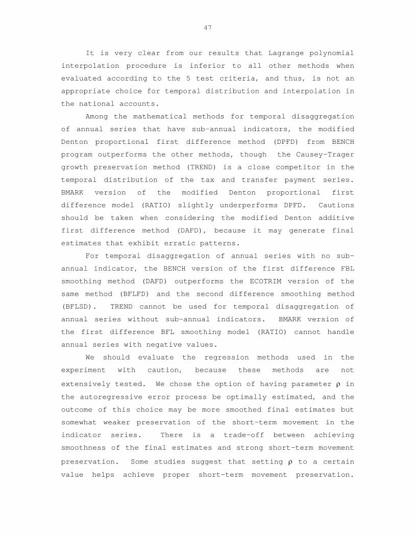
47

It is very clear from our results that Lagrange polynomial

interpolation procedure is inferior to all other methods when

evaluated according to the 5 test criteria, and thus, is not an

appropriate choice for temporal distribution and interpolation in

the national accounts.

Among the mathematical methods for temporal disaggregation

of annual series that have sub-annual indicators, the modified

Denton proportional first difference method (DPFD) from BENCH

program outperforms the other methods, though the Causey-Trager

growth preservation method (TREND) is a close competitor in the

temporal distribution of the tax and transfer payment series.

BMARK version of the modified Denton proportional first

difference model (RATIO) slightly underperforms DPFD. Cautions

should be taken when considering the modified Denton additive

first difference method (DAFD), because it may generate final

estimates that exhibit erratic patterns.

For temporal disaggregation of annual series with no sub-

annual indicator, the BENCH version of the first difference FBL

smoothing method (DAFD) outperforms the ECOTRIM version of the

same method (BFLFD) and the second difference smoothing method

(BFLSD). TREND cannot be used for temporal disaggregation of

annual series without sub-annual indicators. BMARK version of

the first difference BFL smoothing model (RATIO) cannot handle

annual series with negative values.

We should evaluate the regression methods used in the

experiment with caution, because these methods are not

extensively tested. We chose the option of having parameter ρ in

the autoregressive error process be optimally estimated, and the

outcome of this choice may be more smoothed final estimates but

somewhat weaker preservation of the short-term movement in the

indicator series. There is a trade-off between achieving

smoothness of the final estimates and strong short-term movement

preservation. Some studies suggest that setting ρ to a certain

value helps achieve proper short-term movement preservation.

48

More tests with different parameter values should be conducted to

reach more conclusive evaluation.

We should also point out that the current revision policy

in the national accounts limit the advantages that regression

methods can offer. Most of the series used in the experiment are

clearly serially correlated. Using regression methods to correct

serial correlation should improve the final estimates. However,

because only the most recent 3 years of data can be used in

estimation, it would be very difficult for any regression method

to produce reliable results.

6. Conclusion

We have experimented with 5 mathematical and 5 regression

methods for temporal distribution and interpolation using 3

software programs designed for benchmarking and temporal

disaggregation. Because we have used a large number of series

that allow us to study a variety of cases routinely encountered

in temporal distribution and interpolation at the national

accounts, we have acquired a good understanding of how each

method works in each case. Such knowledge provides us with a

solid basis for selecting the most suitable method(s) for routine

compilation at the national accounts.

This study has also helped familiarize us with the frontier

research in this area. New research on temporal disaggregation

and new software programs developed for that purpose continue to

emerge, which should further benefit our research in the future.

One can see from the estimation results that the mathematical

methods are easier to use, but they do not correct any serial

correlation in the time-series data. Thus, in our future

research, we would like to further examine regression-based

methods which would help correct serial correlation in the time-

series data. The best method for temporal disaggregation at the

national accounts should produces sub-annual estimates that

49

satisfy the criteria used in our evaluation and are also free of

serial correlation. Toward that goal we shall continue our

research.

References Aadland, D.M. (2000), “Distribution and interpolation using

transformed data,” Journal of Applied Statistics 27, pp. 141-156.

Bassie, V.L. (1958), Economic Forecasting, Appendix A,

“Interpolation formulas for the adjustment of index numbers.” McGraw-Hill, New York.

Bloem, A.M., Dippelsman, R.J., Maehle, O.N. (2001) Quarterly

National Accounts Manual: Concepts, Data Sources, and Compilation, International Monetary Fund, Washington, DC.

Boot, J.C.G., Feibes, W., Lisman, J.H.C. (1967), “Further methods

of derivation of quarterly figures from annual data.” Applied Statistics 16(1), pp. 65-75.

Bournay, J., Laroque, G. (1979), Reflexions sur la methode

d’elaboration des comptes trimestriels.” Annuales de I’I.N.S.E. 36, pp. 3-30.

Bozik, J.E., Otto, M.C. (1988), “Benchmarking: Evaluating Methods

that preserve month-to-month changes,” Statistical Research Division Report Series RR-88-07, Bureau of the Census.

Causey, B. and M.L. Trager (1981), “Derivation of solution to the

benchmarking problem: Trend revision,” Unpublished research notes, U.S. Census Bureau.

Chen, Z.G., Cholette, P.A., Dagum, E. Bee (1997), “A

nonparametric method for benchmarking survey data via signal extraction,” Journal of the American Statistical Association 92, pp. 1563-1571.

Cholette, P.A., Dagum, E. Bee (1994), “Benchmarking time series

with autocorrelated sampling errors,” International Statistical Review 63, pp. 365-377.

Cholette, P.A. (2001), User’s Manual of Programme BENCH to

Benchmark, Interpolate and Calendarize Time-Series Data on Microcomputer, Statistics Canada, Time Series Research and Analysis Division.

50

Cholette, P.A., Dagum, E. Bee (2006), Benchmarking, Temporal Distribution, and Reconciliation Methods of Time Series, Lecture Notes in Statistics 186, Springer Science+Business Media, LLC, New York.

Chow, G.C., Lin, A.L. (1971), “Best linear unbiased

interpolation, distribution and extrapolation of time series by related series,” The review of Economics and Statistics 53, pp. 372-375.

Di Fonzo, T. (2003), “Temporal disaggregation of economic time

series: toward a dynamic extension,” Dipartimento di Scienze Statische, Universita di Padova.

Denton, F.T., (1971), “Adjustment of monthly or quarterly series

to annual totals: An approach based on quadratic minimization,” Journal of the American Statistical Association 66(333), pp. 99-102.

Durbin, J., Quenneville, B. (1997), “Benchmarking by state space

models,” International Statistical Review 65, pp. 23-48. Eurostat (1999), Handbook on Quarterly National Accounts, Office

for Official Publications of the European Communities. Fernadez, R.B. (1981), “A methodological note on the estimation

of time series,” The Review of Economics and Statistics 63(3), pp. 471-476.

Gomez, V. (2000), “Estimating missing observations in ARIMA

models with the Kalman filter,” Annali di Statistica, Rome, Istat.

Gudmundson, G. (1999), “Disaggregation of annual flow data with

multiplicative trends,” Journal of Forecasting 18, pp. 33-37. Harvey, A.C., Pierse, R.G. (1984), “Estimating missing

observations in economic time series,” Journal of the American Statistical Association 79, pp. 125-131.

Helfand, S.D., Monsour, J.J., Trager, M.L. (1977), “Historical

revision of current business survey estimates,” Proceedings of the Business and Economics Statistics Section, American Statistical Association, pp. 246-250.

Hillmer S.C., Trabelsi, A. (1987), “Benchmarking of economic time

series,” Journal of the American Statistical Association 82, pp. 1064-1071.

51

Hood, C.C. (2005), “An Empirical Comparison of Methods for Benchmarking seasonally adjusted series to annual totals,” Proceedings of Business and Economic Statistics Section, American Statistical Association.

Hotta, L.K., Vasconellos, K.L. (1999), “Aggregation and

disaggregation of structural time series models,” Journal of Time Series Analysis 20, pp. 155-171.

Klick, J. (2000), “Proposal for a New Interpolation Methodology,”

Unpublished research notes, Bureau of Economic Analysis. Litterman, R.B. (1983), “A random walk, markov model for the

distribution of time series,” Journal of Business and Statistics, 1, pp. 169-173.

Loebach, L. (2002), “Second order interpolation method,”

Unpublished research notes, Bureau of Economic Analysis. Proietti, T. (1999), “Distribution and interpolation revisited: a

structural approach,” Statistica 58, pp. 411-432. Rossi, N. (1982), “A note on the estimation of disaggregated time

series when the aggregate is known,” The Review of Economics and Statistics 64(4), pp. 695-696.

Stram, D.O., Wei, W.W. (1986), “Temporal aggregation in the ARIMA

process,” Journal of Time Series Analysis 7, pp. 279-292. Trager, M.L. (1982), “Derivation of solution to the benchmarking

problem” relative revision,” Unpublished research notes, U.S. Census Bureau.

Wei, W.W., Stram, D.O. (1990), “Disaggregation of time series

models,” Journal of the Royal Statistical Society, Series B 52, pp. 453-467.

52

Figure 1-1: Annual, Indicator and Interpolated SeriesMonetary Interests (MIRPERSON 1995-2004)

400000

450000

500000

550000

600000

650000

700000

750000

800000

Jan-9 5Apr-9

5Jul-95

O ct-95

Jan-9 6Apr-9

6Jul-96

O ct-96Jan-9 7

Apr-97Jul-97

O ct-97Jan-9 8

Apr-98Jul-98

O ct-98

Jan-9 9Apr-9

9Jul-99

O ct-99

Jan-0 0Apr-0

0Jul-00

O ct-00

Jan-0 1Apr-0

1Jul-01

O ct-01Jan-0 2

Apr-02Jul-02

O ct-02Jan-0 3

Apr-03Jul-03

O ct-03

Jan-0 4Apr-0

4Jul-04

O ct-04

time

Qua

rter

ly E

stim

ates

INDICATOR* Annual LPI DPFD RATIO TREND

Figure 1-2: Annual, Indicator and Interpolated SeriesHousing owner occupied closing cost (XOTHOTHCCO 1995-2004)

0

5000

10000

15000

20000

25000

30000

35000

40000

Jan-9 5Apr-9

5Jul-95

Oct-95Jan-9 6

Apr-96Jul-96

Oct-96Jan-97

Apr-97Jul-97

Oct-97Jan-9 8

Apr-98Jul-98

Oct-98Jan-9 9

Apr-99Jul-99

Oct-99Jan-0 0

Apr-00Jul-00

Oct-00Jan-01

Apr-01Jul-01

Oct-01Jan-0 2

Apr-02Jul-02

Oct-02Jan-0 3

Apr-03Jul-03

Oct-03Jan-0 4

Apr-04Jul-04

Oct-04

time

Qua

rter

ly E

stim

ates

INDICATOR* Annual LPI DPFD RATIO TREND

53

Figure 1-3: Annual, Indicator and Interpolated SeriesCrop Output (GFOCXLOSS 1994-2004 (revised data))

75000

80000

85000

90000

95000

100000

105000

Jan-9 4Apr-9

4Jul-94

O ct-94

Jan-9 5Apr-9

5Jul-95

O ct-95

Jan-9 6Apr-9

6Jul-96

O ct-96

Jan-9 7Apr-9

7Jul-97

O ct-97

Jan-9 8Apr-9

8Jul-98

O ct-98

Jan-9 9Apr-9

9Jul-99

O ct-99

Jan-0 0Apr-0

0Jul-00

O ct-00

Jan-0 1Apr-0

1Jul-01

O ct-01

Jan-0 2Apr-0

2Jul-02

O ct-02

Jan-0 3Apr-0

3Jul-03

O ct-03

Jan-0 4Apr-0

4Jul-04

O ct-04

time

Qua

rter

ly E

stim

ates

INDICATOR* Annual LPI DPFD DAFD RATIO TREND

Figure 1-4: Annual, Indicator and Interpolated SeriesOwner-Occupied Mobile Homes (EOMHP 1995-2004 revised data)

20000

24000

28000

32000

36000

40000

Jan-95Apr-9

5Jul-9

5Oct-

95Jan-96

Apr-96Jul-9

6Oct-

96Jan-97

Apr-97Jul-9

7Oct-

97Jan-98

Apr-98Jul-9

8Oct-

98Jan-99

Apr-99Jul-9

9Oct-

99Jan-00

Apr-00Jul-0

0Oct-

00Jan-01

Apr-01Jul-0

1Oct-

01Jan-02

Apr-02Jul-0

2Oct-

02Jan-03

Apr-03Jul-0

3Oct-

03Jan-04

Apr-04Jul-0

4Oct-

04

time

Mon

thly

Est

imat

es

INDICATOR* Annual LPI DPFD DAFD RATIO TREND

54

Figure 1-5: Annual, Indicator and Interpolated SeriesTennant-Occupied Mobile Homes (ETMHP 1995-2004 revised data)

4700

4900

5100

5300

5500

5700

5900

6100

6300

Jan-9 5Apr-9

5Jul-95

Oct-95

Jan-9 6Apr-9

6Jul-96

Oct-96Jan-97

Apr-97Jul-97

Oct-97Jan-98

Apr-98Jul-98

Oct-98

Jan-99Apr-9

9Jul-99

Oct-99Jan-00

Apr-00Jul-00

Oct-00Jan-0 1

Apr-01Jul-01

Oct-01

Jan-02Apr-0

2Jul-02

Oct-02

Jan-03Apr-0

3Jul-03

Oct-03Jan-04

Apr-04Jul-04

Oct-04

time

Mon

thly

Est

imat

es

INDICATOR* Annual LPI DPFD DAFD RATIO TREND

Figure 1-6: Annual, Indicator and Interpolated Series

Livestock Output (GFOL$ 1994-2004 revised data)

80000

85000

90000

95000

100000

105000

110000

115000

Jan-94Apr-9

4Jul-9

4Oct-9

4Jan-9 5

Apr-95Jul-9

5Oct-9

5Jan-9 6

Apr-96Jul-9

6Oct-9

6Jan-9 7

Apr-97Jul-9

7Oct-9

7Jan-9 8

Apr-98Jul-9

8Oct-9

8Jan-99

Apr-99Jul-9

9Oct-9

9Jan-0 0

Apr-00Jul-0

0Oct-0

0Jan-0 1

Apr-01Jul-0

1Oct-0

1Jan-0 2

Apr-02Jul-0

2Oct-0

2Jan-0 3

Apr-03Jul-0

3Oct-0

3

time

Qua

rter

ly E

stim

ates

INDICATOR* Annual LPI DPFD DAFD RATIO TREND

55

Figure 1-7a: Annual, Indicator and Interpolated SeriesGasoline Consumption (E1GAS1 1993-2004)

0

50000

100000

150000

200000

250000

300000

350000

400000

450000

Jan-9 3Apr-9

3Jul-93

Oct-93

Jan-9 4Apr-9

4Jul-94

Oct-94

Jan-9 5Apr-9

5Jul-95

Oct-95

Jan-9 6Apr-9

6Jul-96

Oct-96

Jan-9 7Apr-9

7Jul-97

Oct-97

Jan-9 8Apr-9

8Jul-98

Oct-98

Jan-9 9Apr-9

9Jul-99

Oct-99

Jan-0 0Apr-0

0Jul-00

Oct-00

Jan-0 1Apr-0

1Jul-01

Oct-01

Jan-0 2Apr-0

2Jul-02

Oct-02

Jan-0 3Apr-0

3Jul-03

Oct-03

Jan-0 4Apr-0

4Jul-04

Oct-04

time

Mon

thly

Est

imat

es

INDICATOR* Annual LPI DPFD DAFD RATIO TREND

Figure 1-7b: Annual, Indicator and Interpolated SeriesGasoline Consumption (E1GAS1 1993-2004)

100000

120000

140000

160000

180000

200000

220000

240000

Jan-93Apr-9

3Jul-93

Oct-93

Jan-94Apr-9

4Jul-94

Oct-94

Jan-9 5Apr-9

5Jul-95

Oct-95

Jan-96Apr-9

6Jul-96

Oct-96

Jan-97Apr-9

7Jul-97

Oct-97

Jan-9 8Apr-9

8Jul-98

Oct-98

Jan-9 9Apr-9

9Jul-99

Oct-99

Jan-00Apr-0

0Jul-00

Oct-00

Jan-01Apr-0

1Jul-01

Oct-01

Jan-02Apr-0

2Jul-02

Oct-02

Jan-03Apr-0

3Jul-03

Oct-03

Jan-04Apr-0

4Jul-04

Oct-04

time

Mon

thly

Est

imat

es

INDICATOR* Annual LPI DPFD RATIO TREND

56

Figure 1-8a: Annual, Indicator and Interpolated SeriesInvestment in Pre-Packaged Equipment & Software (SFTWRE 1997-2004)

-1000

-500

0

500

1000

1500

Jan-9 7Apr-9

7Jul-97

Oct-97Jan-9 8

Apr-98

Jul-98Oct-9

8Jan-9 9

Apr-99

Jul-99Oct-9

9Jan-0 0

Apr-00Jul-00

Oct-00Jan-0 1

Apr-01Jul-01

Oct-01Jan-0 2

Apr-02

Jul-02Oct-0

2Jan-0 3

Apr-03

Jul-03Oct-0

3Jan-0 4

Apr-04Jul-04

Oct-04

time

Qua

rter

ly E

stim

ates

INDICATOR* Annual LPI DPFD DAFD RATIO TREND

Figure 1-8b: Annual, Indicator and Interpolated SeriesInvestment in Pre-Packaged Equipment & Software (SFTWRE 1997-2004)

30

35

40

45

50

55

60

Jan-9 7Apr-9

7Jul-9

7Oct-9

7Jan-98

Apr-98Jul-9

8Oct-9

8Jan-99

Apr-99Jul-9

9Oct-9

9Jan-0 0

Apr-00Jul-0

0Oct-0

0Jan-0 1

Apr-01Jul-0

1Oct-0

1Jan-02

Apr-02Jul-0

2Oct-0

2Jan-03

Apr-03Jul-0

3Oct-0

3Jan-0 4

Apr-04Jul-0

4Oct-0

4

time

Qua

rter

ly E

stim

ates

INDICATOR* Annual LPI DPFD RATIO TREND

57

Figure 1-9: Annual, Indicator and Interpolated SeriesGasoline Consumption (E1GAS1 1993-2004)

0

50000

100000

150000

200000

250000

300000

Jan-9 3Apr-9

3Jul-93

Oct-93

Jan-9 4Apr-9

4Jul-94

Oct-94

Jan-9 5Apr-9

5Jul-95

Oct-95

Jan-9 6Apr-9

6Jul-96

Oct-96

Jan-9 7Apr-9

7Jul-97

O ct-97

Jan-9 8Apr-9

8Jul-98

Oct-98

Jan-9 9Apr-9

9Jul-99

Oct-99

Jan-0 0Apr-0

0Jul-00

O ct-00

Jan-0 1Apr-0

1Jul-01

Oct-01

Jan-0 2Apr-0

2Jul-02

Oct-02

Jan-0 3Apr-0

3Jul-03

Oct-03

Jan-0 4Apr-0

4Jul-04

Oct-04

time

Mon

thly

Est

imat

es

AR(1) MAX Annual RAWK RAWKM MAX AR(1) MIN RAWKM MIN INDICATOR* LPI

Figure 1-10: Annual, Indicator and Interpolated SeriesNonresidential Telecommunications (CURTUM 1993-2004)

0

5000

10000

15000

20000

25000

Jan-9 3Apr-9

3Jul-93

Oct-93

Jan-9 4Apr-9

4Jul-94

Oct-94

Jan-9 5Apr-9

5Jul-95

Oct-95

Jan-9 6Apr-9

6Jul-96

Oct-96

Jan-9 7Apr-9

7Jul-97

Oct-97

Jan-9 8Apr-9

8Jul-98

Oct-98

Jan-9 9Apr-9

9Jul-99

Oct-99

Jan-0 0Apr-0

0Jul-00

Oct-00

Jan-0 1Apr-0

1Jul-01

Oct-01

Jan-0 2Apr-0

2Jul-02

Oct-02

Jan-0 3Apr-0

3Jul-03

Oct-03

Jan-0 4Apr-0

4Jul-04

Oct-04

time

Mon

thly

Est

imat

es

INDICATOR* Annual LPI AR(1) MAX RAWK RAWKM MAX AR(1) MIN RAWKM MIN

58

Figure 2-1: Absolute difference in period-to-period growth rateMonetary Interest (MIRPERSON 1995-2004)

0.00

0.01

0.01

0.02

0.02

0.03

0.03

0.04

0.04

0.05

0.05

Jan-9 5Apr-9

5Jul-95

Oct-95

Jan-9 6Apr-9

6Jul-96

Oct-96Jan-9 7

Apr-97Jul-97

Oct-97Jan-9 8

Apr-98Jul-98

Oct-98Jan-99

Apr-99Jul-99

Oct-99Jan-0 0

Apr-00Jul-00

Oct-00Jan-0 1

Apr-01Jul-01

Oct-01Jan-0 2

Apr-02Jul-02

Oct-02Jan-0 3

Apr-03Jul-03

Oct-03

Jan-0 4Apr-0

4Jul-04

Oct-04

time

Prop

ortio

nal C

orre

ctio

n

LPI DPFD RATIO TREND

Figure 2-2: Absolute difference in period-to-period growth rateHousing Owner-Occupied Closing Cost (XOTHOTHCCO 1995-2005)

0.00

0.05

0.10

0.15

0.20

0.25

0.30

Jan-95

Apr-95Jul-9

5Oct-

95Jan-96

Apr-96Jul-9

6Oct-

96Jan-97

Apr-97Jul-9

7Oct-

97Jan-98

Apr-98Jul-9

8Oct-

98Jan-99

Apr-99Jul-9

9Oct-

99Jan-00

Apr-00Jul-0

0Oct-

00Jan-01

Apr-01Jul-0

1Oct-

01Jan-02

Apr-02Jul-0

2Oct-

02Jan-03

Apr-03Jul-0

3Oct-

03Jan-04

Apr-04Jul-0

4Oct-

04Jan-05

Apr-05Jul-0

5Oct-

05

time

Prop

ortio

nal C

orre

ctio

n

DPFD RATIO TREND

59

Figure 2-3: Absolute Difference in Period-to-Period Growth RateOwner-Occupied Stationary Homes (EOSTP 1995-2004 revised data)

0

0.0005

0.001

0.0015

0.002

0.0025

0.003

0.0035

Jan-9 5Apr-9

5Jul-95

Oct-95Jan-9 6

Apr-96Jul-96

Oct-96Jan-9 7

Apr-97Jul-97

Oct-97Jan-9 8

Apr-98Jul-98

Oct-98Jan-9 9

Apr-99Jul-99

Oct-99Jan-0 0

Apr-00Jul-00

Oct-00Jan-0 1

Apr-01Jul-01

Oct-01Jan-0 2

Apr-02Jul-02

Oct-02Jan-0 3

Apr-03Jul-03

Oct-03Jan-0 4

Apr-04Jul-04

Oct-04

time

Prop

ortio

nal C

orre

ctio

n

LPI DPFD DAFD RATIO TREND

Figure 2-4: Absolute Difference in Period-to-Period Growth RateTennant-Occupied Mobile Homes (ETMHP 1995-2004 revised data)

0

0.005

0.01

0.015

0.02

0.025

Jan-9 5Apr-9

5Jul-95

Oct-95Jan-9 6

Apr-96Jul-96

Oct-96Jan-9 7

Apr-97Jul-97

Oct-97Jan-9 8

Apr-98Jul-98

Oct-98Jan-9 9

Apr-99Jul-99

Oct-99Jan-0 0

Apr-00Jul-00

Oct-00Jan-0 1

Apr-01Jul-01

Oct-01Jan-0 2

Apr-02Jul-02

Oct-02Jan-0 3

Apr-03Jul-03

Oct-03Jan-0 4

Apr-04Jul-04

Oct-04

time

Prop

ortio

nal C

orre

ctio

n

LPI DPFD DAFD RATIO TREND

60

Figure 2-5: Absolute Difference in Period-to-Period Growth RateCrop Output (GFOCXLOSS$ 1994-2004 revised data)

0

0.005

0.01

0.015

0.02

0.025

0.03

Jan-9 4Apr-9

4Jul-94

Oct-94

Jan-9 5Apr-9

5Jul-95

Oct-95

Jan-9 6Apr-9

6Jul-96

Oct-96

Jan-9 7Apr-9

7Jul-97

Oct-97

Jan-9 8Apr-9

8Jul-98

Oct-98

Jan-9 9Apr-9

9Jul-99

Oct-99

Jan-0 0Apr-0

0Jul-00

Oct-00

Jan-0 1Apr-0

1Jul-01

Oct-01

Jan-0 2Apr-0

2Jul-02

Oct-02

Jan-0 3Apr-0

3Jul-03

Oct-03

Jan-0 4Apr-0

4Jul-04

Oct-04

time

Prop

ortio

nal C

orre

ctio

n

LPI DPFD DAFD RATIO TREND

Figure 2-6: Absolute Difference in Period-to-Period Growth Rate

Livestock Output (GFOL$ 1994-2004 revised data)

0.000

0.020

0.040

0.060

0.080

0.100

0.120

0.140

0.160

0.180

Jan-9 4Apr-9

4Jul-94

Oct-94Jan-9 5

Apr-95Jul-95

Oct-95Jan-9 6

Apr-96Jul-96

Oct-96Jan-9 7

Apr-97Jul-97

Oct-97Jan-9 8

Apr-98Jul-98

Oct-98Jan-9 9

Apr-99Jul-99

Oct-99Jan-00

Apr-00Jul-00

Oct-00Jan-0 1

Apr-01Jul-01

Oct-01Jan-0 2

Apr-02Jul-02

Oct-02Jan-03

Apr-03Jul-03

Oct-03

time

Prop

ortio

nal C

orre

ctio

n

LPI DPFD DAFD RATIO TREND

61

Figure 2-7: Absolute Difference in Period-to-Period Growth RateNonresidential Telecommunications (CURTUM 1993-2004)

0

0.01

0.02

0.03

0.04

0.05

0.06

0.07

0.08

0.09

Jan-9 3Apr-9

3Jul-93

Oct-93

Jan-9 4Apr-9

4Jul-94

Oct-94

Jan-9 5Apr-9

5Jul-95

Oct-95

Jan-9 6Apr-9

6Jul-96

Oct-96

Jan-9 7Apr-9

7Jul-97

Oct-97

Jan-9 8Apr-9

8Jul-98

Oct-98

Jan-9 9Apr-9

9Jul-99

Oct-99

Jan-0 0Apr-0

0Jul-00

Oct-00

Jan-0 1Apr-0

1Jul-01

Oct-01

Jan-0 2Apr-0

2Jul-02

Oct-02

Jan-0 3Apr-0

3Jul-03

Oct-03

Jan-0 4Apr-0

4Jul-04

Oct-04

time

Prop

ortio

nal C

orre

ctio

n

LPI DPFD DAFD RATIO TREND

Figure 2-8: Absolute Difference in Period-to-Period Growth RateNonresidential Manufacturing (CURMFG 1993-2004)

0

0.01

0.02

0.03

0.04

0.05

0.06

0.07

Jan-9 3Apr-9

3Jul-93

Oct-93

Jan-9 4Apr-9

4Jul-94

Oct-94

Jan-9 5Apr-9

5Jul-95

Oct-95

Jan-9 6Apr-9

6Jul-96

Oct-96

Jan-9 7Apr-9

7Jul-97

Oct-97

Jan-9 8Apr-9

8Jul-98

Oct-98

Jan-9 9Apr-9

9Jul-99

Oct-99

Jan-0 0Apr-0

0Jul-00

Oct-00

Jan-0 1Apr-0

1Jul-01

Oct-01

Jan-0 2Apr-0

2Jul-02

Oct-02

Jan-0 3Apr-0

3Jul-03

Oct-03

Jan-0 4Apr-0

4Jul-04

Oct-04

time

Prop

ortio

nal C

orre

ctio

n

LPI DPFD DAFD RATIO TREND

62

Figure 2-9a: Absolute Difference in Period-to-Period Growth RateGasoline Consumption (E1GAS1 1993-2004)

0.00

1.00

2.00

3.00

4.00

5.00

6.00

7.00

8.00

9.00

10.00

Jan-9 3Apr-9

3Jul-93

Oct-93

Jan-9 4Apr-9

4Jul-94

Oct-94

Jan-9 5Apr-9

5Jul-95

Oct-95

Jan-9 6Apr-9

6Jul-96

Oct-96

Jan-9 7Apr-9

7Jul-97

Oct-97

Jan-9 8Apr-9

8Jul-98

Oct-98

Jan-9 9Apr-9

9Jul-99

Oct-99

Jan-0 0Apr-0

0Jul-00

Oct-00

Jan-0 1Apr-0

1Jul-01

Oct-01

Jan-0 2Apr-0

2Jul-02

Oct-02

Jan-0 3Apr-0

3Jul-03

Oct-03

Jan-0 4Apr-0

4Jul-04

Oct-04

time

Prop

ortio

nal C

orre

ctio

n

LPI DPFD RATIO TREND DAFD

Figure 2-9b: Absolute Difference in Period-to-Period Growth Rate

Gasoline Consumption (E1GAS1 1993-2004)

0.00

0.01

0.01

0.02

0.02

0.03

0.03

0.04

0.04

0.05

0.05

Jan-9 3Apr-9

3Jul-93

Oct-93

Jan-9 4Apr-9

4Jul-94

Oct-94

Jan-95Apr-9

5Jul-95

Oct-95

Jan-9 6Apr-9

6Jul-96

Oct-96

Jan-9 7Apr-9

7Jul-97

Oct-97

Jan-9 8Apr-9

8Jul-98

Oct-98

Jan-9 9Apr-9

9Jul-99

Oct-99

Jan-0 0Apr-0

0Jul-00

Oct-00

Jan-0 1Apr-0

1Jul-01

Oct-01

Jan-0 2Apr-0

2Jul-02

Oct-02

Jan-0 3Apr-0

3Jul-03

Oct-03

Jan-0 4Apr-0

4Jul-04

Oct-04

time

Prop

ortio

nal C

orre

ctio

n

LPI DPFD RATIO TREND

63

Figure 2-10a: Absolute Difference in Period-to-Period Growth RateInvestment in Pre-Packaged Equipment & Software (SFTWRE 1997-2004)

0.00

20.00

40.00

60.00

80.00

100.00

120.00

Jan-9 7Apr-9

7Jul-97

O ct-97Jan-9 8

Apr-98Jul-98

O ct-98Jan-9 9

Apr-99Jul-99

O ct-99Jan-0 0

Apr-00Jul-00

O ct-00Jan-0 1

Apr-01Jul-01

O ct-01Jan-0 2

Apr-02Jul-02

O ct-02Jan-0 3

Apr-03Jul-03

O ct-03Jan-0 4

Apr-04Jul-04

O ct-04

time

Prop

ortio

nal C

orre

ctio

n

LPI DPFD RATIO TREND DAFD

Figure 2-10b: Absolute Difference in Period-to-Period Growth RateInvestment in Pre-Packaged Equipment & Software (SFTWRE 1997-2004)

-0.01

0.00

0.01

0.01

0.02

0.02

0.03

0.03

0.04

0.04

0.05

Jan-9 7Apr-9

7Jul-97

Oct-97Jan-9 8

Apr-98Jul-98

Oct-98Jan-9 9

Apr-99Jul-99

Oct-99Jan-0 0

Apr-00Jul-00

Oct-00Jan-0 1

Apr-01Jul-01

O ct-01Jan-0 2

Apr-02Jul-02

Oct-02Jan-0 3

Apr-03Jul-03

Oct-03Jan-0 4

Apr-04Jul-04

Oct-04

time

Prop

ortio

nal C

orre

ctio

n

LPI DPFD RATIO TREND

64

Figure 2-11: Absolute Difference in Period-to-Period Growth RateTennant-Occupied Mobile Homes (ETMHP 1995-2004 revised data)

0

0.001

0.002

0.003

0.004

0.005

0.006

0.007

0.008

0.009

Jan-9 5Apr-9

5Jul-9

5Oct-

95Jan-96

Apr-96Jul-9

6Oct-

96Jan-97

Apr-97Jul-9

7Oct-

97Jan-9 8

Apr-98Jul-9

8Oct-

98Jan-9 9

Apr-99Jul-9

9Oct-

99Jan-00

Apr-00Jul-0

0Oct-

00Jan-01

Apr-01Jul-0

1Oct-

01Jan-0 2

Apr-02Jul-0

2Oct-

02Jan-03

Apr-03Jul-0

3Oct-

03Jan-04

Apr-04Jul-0

4Oct-

04

time

Prop

ortio

nal C

orre

ctio

n

AR(1) MAX RAWK RAWKM MAX AR(1) MIN RAWKM MIN

Figure 2-12: Absolute Difference in Period-to-Period Growth RateCrop Output (GFOCXLOSS 1994-2004 revised data)

0

0.005

0.01

0.015

0.02

0.025

0.03

Jan-94

Apr-94Jul-9

4

Oct-94Ja

n-95

Apr-95Ju

l-95

Oct-95Jan-9

6

Apr-96Jul-

96

Oct-96Ja

n-97

Apr-97Jul-9

7

Oct-97Jan

-98

Apr-98Jul-

98

Oct-98Ja

n-99

Apr-99Jul-9

9

Oct-99Jan

-00

Apr-00Ju

l-00

Oct-00Jan-0

1

Apr-01Jul-0

1

Oct-01Ja

n-02

Apr-02Ju

l-02

Oct-02Jan-0

3

Apr-03Jul-

03

Oct-03Ja

n-04

Apr-04Jul-0

4

Oct-04

time

Prop

ortio

nal C

orre

ctio

n

AR(1) MAX RAWK RAWKM MAX AR(1) MIN RAWKM MIN LIP

65

Figure 2-13: Absolute Difference in Period-to-Period Growth RateGasoline Consumption (E1GAS1 1993-2004)

0

0.001

0.002

0.003

0.004

0.005

0.006

0.007

Jan-9 3

Apr-93

Jul-93

Oct-93Jan-94

Apr-94

Jul-94

Oct-94Jan-95

Apr-95Jul-9

5Oct-

95Jan-96

Apr-96Jul-9

6Oct-

96Jan-97

Apr-97

Jul-97

Oct-97Jan-9 8

Apr-98

Jul-98

Oct-98Jan-9 9

Apr-99Jul-9

9Oct-

99Jan-0 0

Apr-00Jul-0

0Oct-

00Jan-01

Apr-01

Jul-01

Oct-01Jan-02

Apr-02

Jul-02

Oct-02Jan-03

Apr-03Jul-0

3Oct-

03Jan-04

Apr-04Jul-0

4Oct-

04

time

Prop

ortio

nal C

orre

ctio

n

AR(1) MAX RAWK RAWKM MAX AR(1) MIN RAWKM MIN

Figure 2-14: Absolute Difference in Period-to-Period Growth RateNonresidential Telecommunications (CURTUM 1993-2004)

0

0.002

0.004

0.006

0.008

0.01

0.012

0.014

Jan-93

Apr-93Jul-9

3Oct-

93Jan-94

Apr-94Jul-9

4Oct-

94Jan-95

Apr-95

Jul-95

Oct-95Jan-96

Apr-96Jul-9

6Oct-

96Jan-97

Apr-97Jul-9

7Oct-

97Jan-98

Apr-98Jul-9

8Oct-

98Jan-99

Apr-99Jul-9

9Oct-

99Jan-00

Apr-00Jul-0

0Oct-

00Jan-01

Apr-01Jul-0

1Oct-

01Jan-02

Apr-02Jul-0

2Oct-

02Jan-03

Apr-03Jul-0

3Oct-

03Jan-04

Apr-04Jul-0

4Oct-

04

time

Prop

ortio

nal C

orre

ctio

n

AR(1) MAX RAWK RAWKM MAX AR(1) MIN RAWKM MIN

66

Figure 3-1: Absolute Difference in Period-to-Period Growth RateTaxes on Retail Trade (TPCRT 1997-2004)

0.000

0.002

0.004

0.006

0.008

0.010

0.012

0.014

Jan-97

Apr-97Jul-9

7Oct-

97Jan-98

Apr-98Jul-

98Oct-

98Jan-99

Apr-99Jul-9

9Oct-

99Jan-0

0

Apr-00

Jul-0

0Oct-

00Jan-01

Apr-01Jul-0

1Oct-

01Jan

-02

Apr-02Ju

l-02Oct-

02Jan-03

Apr-03Jul-0

3Oct-

03Ja

n-04

Apr-04Jul-0

4Oct-

04

time

Prop

ortio

nal C

orre

ctio

n

LPI DPFD RATIO TREND

Figure 3-2: Absolute Difference in Period-to-Period Growth RateTaxes on Wholesale Trade (TPCWT 1997-2004)

0.000

0.002

0.004

0.006

0.008

0.010

0.012

Jan-9

7

Apr-97

Jul-9

7

Oct-97

Jan-9

8

Apr-98

Jul-9

8

Oct-98

Jan-9

9

Apr-99Ju

l-99

Oct-99

Jan-0

0

Apr-00

Jul-0

0

Oct-00

Jan-0

1

Apr-01

Jul-0

1

Oct-01

Jan-0

2

Apr-02Ju

l-02

Oct-02

Jan-0

3

Apr-03

Jul-0

3

Oct-03

Jan-0

4

Apr-04

Jul-0

4

Oct-04

time

Prop

ortio

nal C

orre

ctio

n

LPI DPFD RATIO TREND

67

Figure 3-3: Absolute Difference in Period-to-Period Growth RateTransfers from Mining (TRCMI 1997-2004)

0

0.01

0.02

0.03

0.04

0.05

0.06

Jan-9

7

Apr-97

Jul-9

7

Oct-97Ja

n-98

Apr-98

Jul-9

8

Oct-98Ja

n-99

Apr-99

Jul-9

9

Oct-99Ja

n-00

Apr-00Ju

l-00

Oct-00Jan

-01

Apr-01Jul-

01

Oct-01Jan

-02

Apr-02

Jul-02

Oct-02Ja

n-03

Apr-03

Jul-0

3

Oct-03Ja

n-04

Apr-04

Jul-0

4

Oct-04

time

Prop

ortio

nal C

orre

ctio

n

LPI DPFD RATIO TREND

Figure 3-4: Absolute Difference in Period-to-Period Growth RateTransfers from Transportation and Warehousing (TRCTW 1997-2004)

0.00

0.01

0.02

0.03

0.04

0.05

0.06

Jan-97

Apr-97Jul-9

7

Oct-97Jan-98

Apr-98Jul-9

8

Oct-98Jan-99

Apr-99Jul-

99

Oct-99Jan-00

Apr-00Jul-

00

Oct-00Jan

-01

Apr-01Jul-0

1

Oct-01Jan

-02

Apr-02Jul-0

2

Oct-02Ja

n-03

Apr-03Jul-0

3

Oct-03Ja

n-04

Apr-04Jul-0

4

Oct-04

time

Prop

ortio

nal C

orre

ctio

n

LPI DPFD RATIO TREND

68

Figure 4-1: Final Sub-Annual EstimateTDI Benefits (CGNTRTD 1993-2004)

0500

100015002000

25003000350040004500

Jan-9 3Apr-9

3Jul-93

O ct-93

Jan-9 4Apr-9

4Jul-94

O ct-94

Jan-9 5Apr-9

5Jul-95

O ct-95

Jan-9 6Apr-9

6Jul-96

O ct-96

Jan-9 7Apr-9

7Jul-97

O ct-97

Jan-9 8Apr-9

8Jul-98

O ct-98

Jan-9 9Apr-9

9Jul-99

O ct-99

Jan-0 0Apr-0

0Jul-00

O ct-00

Jan-0 1Apr-0

1Jul-01

O ct-01

Jan-0 2Apr-0

2Jul-02

O ct-02

Jan-0 3Apr-0

3Jul-03

O ct-03

Jan-0 4Apr-0

4Jul-04

O ct-04

time

LPI DAFD BFLFD BFLSD RATIO Annual

Figure 4-2: Final Sub-Annual EstimateOuter Continental Shelf Royalties (IBT811 1993-2004)

0200400600800

100012001400160018002000

Jan-9 3Apr-9

3Jul-93

Oct-93

Jan-9 4Apr-9

4Jul-94

Oct-94

Jan-9 5Apr-9

5Jul-95

Oct-95

Jan-9 6Apr-9

6Jul-96

Oct-96

Jan-9 7Apr-9

7Jul-97

Oct-97

Jan-9 8Apr-9

8Jul-98

Oct-98

Jan-9 9Apr-9

9Jul-99

Oct-99

Jan-0 0Apr-0

0Jul-00

Oct-00

Jan-0 1Apr-0

1Jul-01

Oct-01

Jan-0 2Apr-0

2Jul-02

Oct-02

Jan-0 3Apr-0

3Jul-03

Oct-03

Jan-0 4Apr-0

4Jul-04

Oct-04

time

LPI DAFD BFLFD BFLSD RATIO Annual

69

Figure 4-3: Final Sub-Annual EstimateNonresidential Other Power (CUROTHPOW 1993-2004)

0

2000

4000

6000

8000

10000

12000

Jan-9 3Apr-9

3Jul-93

O ct-93

Jan-9 4Apr-9

4Jul-94

O ct-94

Jan-9 5Apr-9

5Jul-95

O ct-95

Jan-9 6Apr-9

6Jul-96

Oct-96

Jan-9 7Apr-9

7Jul-97

O ct-97

Jan-9 8Apr-9

8Jul-98

O ct-98

Jan-9 9Apr-9

9Jul-99

O ct-99

Jan-0 0Apr-0

0Jul-00

O ct-00

Jan-0 1Apr-0

1Jul-01

O ct-01

Jan-0 2Apr-0

2Jul-02

O ct-02

Jan-0 3Apr-0

3Jul-03

Oct-03

Jan-0 4Apr-0

4Jul-04

Oct-04

time

LPI BFLFD BFLSD RATIO DPFD Annual

Figure 4-4: Final Sub-Annual EstimateMaritime Operating (SUB420 1993-2004)

0

50

100

150

200

250

300

350

Jan-9 3Apr-9

3Jul-93

Oct-93

Jan-9 4Apr-9

4Jul-94

Oct-94

Jan-9 5Apr-9

5Jul-95

Oct-95

Jan-9 6Apr-9

6Jul-96

Oct-96

Jan-9 7Apr-9

7Jul-97

Oct-97

Jan-9 8Apr-9

8Jul-98

Oct-98

Jan-9 9Apr-9

9Jul-99

Oct-99

Jan-0 0Apr-0

0Jul-00

Oct-00

Jan-0 1Apr-0

1Jul-01

Oct-01

Jan-0 2Apr-0

2Jul-02

Oct-02

Jan-0 3Apr-0

3Jul-03

Oct-03

Jan-0 4Apr-0

4Jul-04

Oct-04

time

LPI DAFD BFLFD BFLSD RATIO Annual

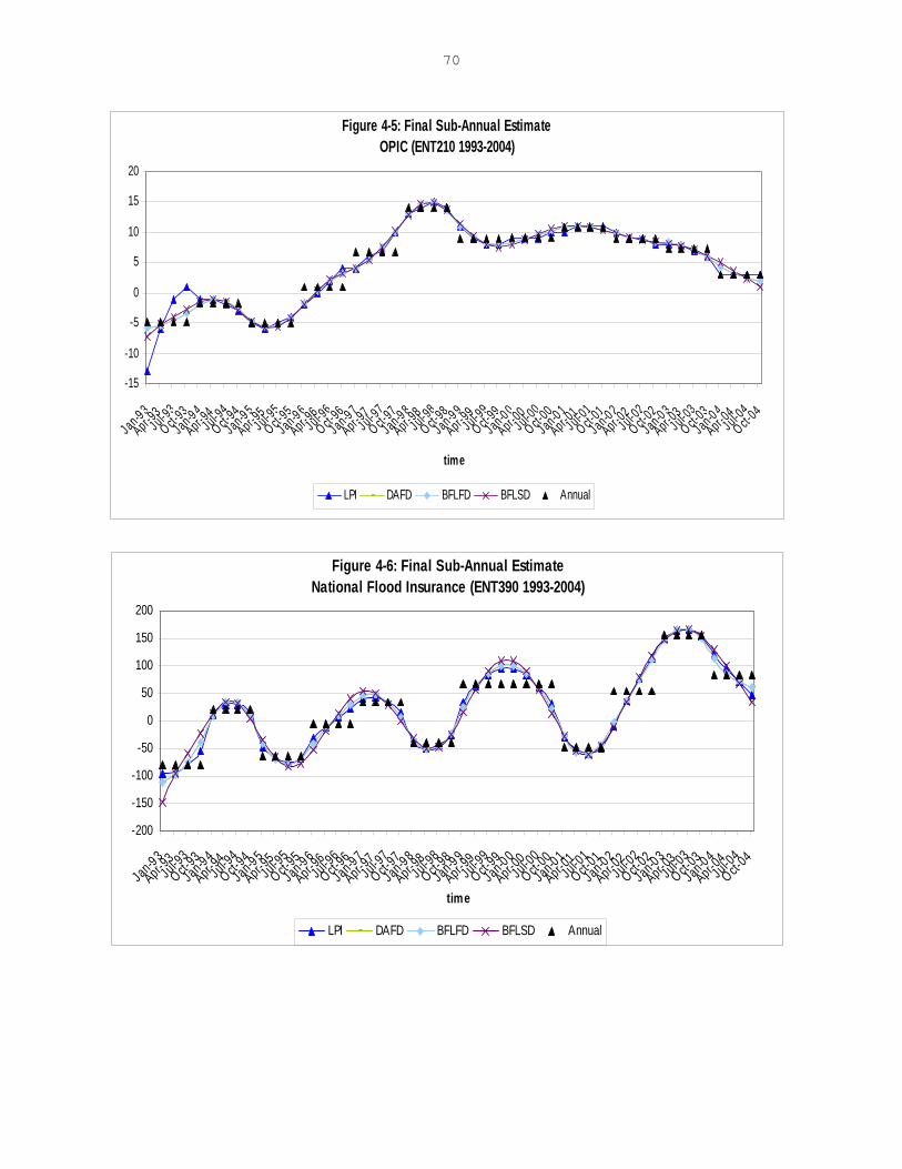
70

Figure 4-5: Final Sub-Annual EstimateOPIC (ENT210 1993-2004)

-15

-10

-5

0

5

10

15

20

Jan-9 3Apr-9

3Jul-93

Oct-93

Jan-9 4Apr-9

4Jul-94

Oct-94

Jan-9 5Apr-9

5Jul-95

Oct-95

Jan-9 6Apr-9

6Jul-96

Oct-96

Jan-9 7Apr-9

7Jul-97

Oct-97

Jan-9 8Apr-9

8Jul-98

Oct-98

Jan-9 9Apr-9

9Jul-99

Oct-99

Jan-0 0Apr-0

0Jul-00

Oct-00

Jan-0 1Apr-0

1Jul-01

Oct-01

Jan-0 2Apr-0

2Jul-02

Oct-02

Jan-0 3Apr-0

3Jul-03

Oct-03

Jan-0 4Apr-0

4Jul-04

Oct-04

time

LPI DAFD BFLFD BFLSD Annual

Figure 4-6: Final Sub-Annual EstimateNational Flood Insurance (ENT390 1993-2004)

-200

-150

-100

-50

0

50

100

150

200

Jan-93Apr-9

3Jul-9

3Oct-

93Jan-94

Apr-94

Jul-94

Oct-94

Jan-95Apr-9

5Jul-9

5Oct-

95Jan-9 6

Apr-96

Jul-96

Oct-96

Jan-9 7Apr-9

7Jul-9

7Oct-

97Jan-98

Apr-98

Jul-98

Oct-98

Jan-99Apr-9

9Jul-9

9Oct-

99Jan-0 0

Apr-00

Jul-00

Oct-00

Jan-0 1Apr-0

1Jul-0

1Oct-

01Jan-02

Apr-02

Jul-02

Oct-02

Jan-03Apr-0

3Jul-0

3Oct-

03Jan-0 4

Apr-04

Jul-04

Oct-04

time

LPI DAFD BFLFD BFLSD Annual

71

Figure 4-7: Period-to-Period Growth Rate TDI Benefits (CGNTRD 1993-2004)

-10-8-6-4-202468

10

Jan-9 3Apr-9

3J ul-93

O ct-93

J an-9 4Apr-9

4Jul-94

O ct-94

Jan-9 5Apr-9

5Jul-95

O ct-95

Jan-9 6Apr-9

6J ul-96

O ct-96

J an-9 7Apr-9

7Jul-97

O ct-97

Jan-9 8Apr-9

8J ul-98

O ct-98

J an-9 9Apr-9

9Jul-99

O ct-99

Jan-0 0Apr-0

0Jul-00

O ct-00

Jan-0 1Apr-0

1Jul-01

O ct-01

Jan-0 2Apr-0

2Jul-02

O ct-02

Jan-0 3Apr-0

3J ul-03

O ct-03

J an-0 4Apr-0

4Jul-04

O ct-04

time

g(t-

1)

LPI DAFD BFLFD BFLSD RATIO

Figure 4-8: Period-to-Period Growth RateOuter Continental Shelf Royalties (IBT811 1993-2004)

-20

-10

0

10

20

30

40

Jan-9 3Apr-9

3Jul-93

Oct-93

Jan-9 4Apr-9

4Jul-94

Oct-94

Jan-9 5Apr-9

5Jul-95

Oct-95

Jan-9 6Apr-9

6Jul-96

Oct-96

Jan-9 7Apr-9

7Jul-97

Oct-97

Jan-9 8Apr-9

8Jul-98

Oct-98

Jan-9 9Apr-9

9Jul-99

Oct-99

Jan-0 0Apr-0

0Jul-00

Oct-00

Jan-0 1Apr-0

1Jul-01

Oct-01

Jan-0 2Apr-0

2Jul-02

Oct-02

Jan-0 3Apr-0

3Jul-03

Oct-03

Jan-0 4Apr-0

4Jul-04

Oct-04

time

g(t-

1)

LPI DAFD BFLFD BFLSD RATIO

72

Figure 4-9: Period-to-Period Growth Rate Nonresidential Other Power (CUROTHPOW 1993-2004)

-40

-30

-20

-10

0

10

20

30

40

50

Jan-9 3Apr-9

3Jul-93

Oct-93

Jan-9 4Apr-9

4Jul-94

Oct-94

Jan-9 5Apr-9

5Jul-95

Oct-95

Jan-9 6Apr-9

6Jul-96

Oct-96

Jan-9 7Apr-9

7Jul-97

Oct-97

Jan-9 8Apr-9

8Jul-98

Oct-98

Jan-9 9Apr-9

9Jul-99

Oct-99

Jan-0 0Apr-0

0Jul-00

Oct-00

Jan-0 1Apr-0

1Jul-01

Oct-01

Jan-0 2Apr-0

2Jul-02

Oct-02

Jan-0 3Apr-0

3Jul-03

Oct-03

Jan-0 4Apr-0

4Jul-04

Oct-04

time

g(t-

1)

LPI BFLFD DFLSD RATIO DPFD

Figure 4-10: Period-to-Period Growth Rate

Maritime Operating (SUB420 1993-2004)

-80-60

-40-20

020

4060

80100

120

Jan-9

3

Apr-93Ju

l-93

Oct-93Ja

n-94

Apr-94Ju

l-94

Oct-94Ja

n-95

Apr-95Ju

l-95

Oct-95Ja

n-96

Apr-96Ju

l-96

Oct-96Ja

n-97

Apr-97Ju

l-97

Oct-97Ja

n-98

Apr-98Ju

l-98

Oct-98Ja

n-99

Apr-99Ju

l-99

Oct-99Ja

n-00

Apr-00Ju

l-00

Oct-00Ja

n-01

Apr-01Ju

l-01

Oct-01Ja

n-02

Apr-02Ju

l-02

Oct-02Ja

n-03

Apr-03Ju

l-03

Oct-03Ja

n-04

Apr-04Ju

l-04

Oct-04

time

g(t-

1)

LPI DAFD BFLFD BFLSD RATIO

73

Figure 4-11: Absolute Period-to-Period Level ChangeOPIC (ENT210 1993-2004)

0

1

2

3

4

5

6

7

8

Jan-9 3Apr-9

3Jul-93

O ct-93

Jan-9 4Apr-9

4Jul-94

O ct-94

Jan-9 5Apr-9

5Jul-95

O ct-95

Jan-9 6Apr-9

6Jul-96

O ct-96

Jan-9 7Apr-9

7Jul-97

O ct-97

Jan-9 8Apr-9

8Jul-98

O ct-98

Jan-9 9Apr-9

9Jul-99

O ct-99

Jan-0 0Apr-0

0Jul-00

O ct-00

Jan-0 1Apr-0

1Jul-01

O ct-01

Jan-0 2Apr-0

2Jul-02

O ct-02

Jan-0 3Apr-0

3Jul-03

O ct-03

Jan-0 4Apr-0

4Jul-04

O ct-04

time

LPI DAFD BFLFD BFLSD

Figure 4-12: Absolute Period-to-Period Level Change

National Flood Insurance (ENT390 1993-2004)

0

10

20

30

40

50

60

70

Jan-93

Apr-93

Jul-93

Oct-93Jan-94

Apr-94

Jul-94

Oct-94

Jan-95

Apr-95

Jul-95

Oct-95

Jan-96

Apr-96Jul-9

6Oct-

96Jan-97

Apr-97

Jul-97

Oct-97

Jan-98

Apr-98

Jul-98

Oct-98Jan-99

Apr-99

Jul-99

Oct-99

Jan-00

Apr-00

Jul-00

Oct-00

Jan-01

Apr-01Jul-0

1Oct-

01Jan-02

Apr-02

Jul-02

Oct-02

Jan-03

Apr-03

Jul-03

Oct-03Jan-04

Apr-04

Jul-04

Oct-04

time

LPI DAFD BFLFD BFLSD

74

Table 1: Correlation Coefficient ρ between Annual and Sub-annual Indicators

Series ρ Series ρ Series ρMIRPERSON 0.8130 TPCAG 0.9516 TRCAG 0.9443

XOTHOTHCOST 0.9236 TPCMI 0.8579 TRCMI 0.8968XOTHOTHCCO 0.9273 TPCUT 0.9844 TRCUT 0.9124GFOCXLOSS 0.9729 TPCAE 0.9918 TRCAE 0.9535

EOMHP 0.8711 TPCCO 0.9970 TRCCO 0.9647EOSTP 0.9994 TPCDG 0.9971 TRCDG 0.9349ETMHP 0.9795 TPCED 0.9954 TRCED 0.9345ETSPP 0.9804 TPCFR 0.9941 TRCFR 0.8286EIGAS1 0.9988 TPCIN 0.9721 TRCIN 0.9698GFOLS 0.9927 TPCNG 0.9773 TRCNG 0.9503

CURMFG 0.9320 TPCOS 0.9985 TRCOS 0.9536CURTUM 0.9996 TPCPF 0.9854 TRCPF 0.9757CURMFU 0.9999 TPCRT 0.9951 TRCRT 0.9473SFTWRE 0.9654 TPCTW 0.9550 TRCTW 0.9519

TPCWT 0.9981 TRCWT 0.9460TPCGV -0.6598

NEA Series Taxes Transfer Payments

Table 2-1: Proportional Discrepancies of NEA Series from All Methods

DzP Dx

P

No. Series IND LPI DPFD DAFD RATIO TREND AR(1)MAX RAWK RAWKM MAX AR(1)MIN RAWKM MIN1 MIRPERSON 1.0502 1.0000 1.0000 1.0000 1.0000 1.0000 1.0000 1.0000 1.0000 1.0000 1.00002 XOTHOTHCOST 0.0399 1.0409 1.0000 1.0000 1.0000 1.0000 1.0000 1.0000 1.0000 1.0000 1.00003 XOTHOTHCCO 0.0339 1.0332 1.0000 1.0000 1.0000 1.0000 1.0000 1.0000 1.0000 1.0000 1.00004 GFOCXLOSS 1.0018 1.0000 1.0000 1.0000 1.0000 1.0000 1.0000 1.0000 1.0000 1.0000 1.00005 EOMHP 1.0240 1.0000 1.0000 1.0000 1.0000 1.0000 1.0000 1.0000 1.0000 1.0000 1.00006 EOSTP 1.0125 1.0000 1.0000 1.0000 1.0000 1.0000 1.0000 1.0000 1.0000 1.0000 1.00007 ETMHP 1.0050 1.0000 1.0000 1.0000 1.0000 1.0000 1.0000 1.0000 1.0000 1.0000 1.00008 ETSPP 0.9768 1.0000 1.0000 1.0000 1.0000 1.0000 1.0000 1.0000 1.0000 1.0000 1.00009 E1GAS1 0.1296 0.8997 1.0000 1.0000 1.0000 1.0000 1.0000 1.0000 1.0000 1.0000 1.0000

10 GFOL 1.0003 1.0000 1.0000 1.0000 1.0000 1.0000 1.0000 1.0000 1.0000 1.0000 1.000011 CURMFG 0.9098 0.9167 1.0000 1.0000 1.0000 1.0000 1.0000 1.0000 1.0000 1.0000 1.000012 CURTUM 1.0008 0.9167 1.0000 1.0000 1.0000 1.0000 1.0000 1.0000 1.0000 1.0000 1.000013 CURMFU 1.0002 0.8997 1.0000 1.0000 1.0000 1.0000 1.0000 1.0000 1.0000 1.0000 1.000014 SFTWRE 0.0021 1.0000 1.0000 1.0000 1.0000 1.0000 1.0000 1.0000 1.0000 1.0000 1.0000

MEAN 0.7276 0.9791 1.0000 1.0000 1.0000 1.0000 1.0000 1.0000 1.0000 1.0000 1.0000 Table 2-2: Proportional Discrepancies of Taxes and Transfers from All Methods

DzP Dx

P DzP Dx

P

No. Series IND LPI DPFD RATIO TREND No. Series IND LPI DPFD RATIO TREND1 TPCAG 0.0079 1.0000 1.0000 1.0000 1.0000 17 TRCAG 0.0051 1.0000 1.0000 1.0000 1.00002 TPCMI 0.0181 1.0000 1.0000 1.0000 1.0000 18 TRCMI 0.0832 1.0000 1.0000 1.0000 1.00003 TPCUT 0.0453 1.0000 1.0000 1.0000 1.0000 19 TRCUT 0.0528 1.0000 1.0000 1.0000 1.00004 TPCAE 0.0565 1.0000 1.0000 1.0000 1.0000 20 TRCAE 0.0189 1.0000 1.0000 1.0000 1.00005 TPCCO 0.0073 1.0000 1.0000 1.0000 1.0000 21 TRCCO 0.0363 1.0000 1.0000 1.0000 1.00006 TPCDG 0.0193 1.0000 1.0000 1.0000 1.0000 22 TRCDG 0.0720 1.0000 1.0000 1.0000 1.00007 TPCED 0.0122 1.0000 1.0000 1.0000 1.0000 23 TRCED 0.0718 1.0000 1.0000 1.0000 1.00008 TPCFR 0.2877 1.0000 1.0000 1.0000 1.0000 24 TRCFR 0.1748 1.0000 1.0000 1.0000 1.00009 TPCIN 0.0496 1.0000 1.0000 1.0000 1.0000 25 TRCIN 0.0429 1.0000 1.0000 1.0000 1.000010 TPCNG 0.0381 1.0000 1.0000 1.0000 1.0000 26 TRCNG 0.2017 1.0000 1.0000 1.0000 1.000011 TPCOS 0.0219 1.0000 1.0000 1.0000 1.0000 27 TRCOS 0.0156 1.0000 1.0000 1.0000 1.000012 TPCPF 0.0299 1.0000 1.0000 1.0000 1.0000 28 TRCPF 0.0899 1.0000 1.0000 1.0000 1.000013 TPCRT 0.1944 1.0000 1.0000 1.0000 1.0000 29 TRCRT 0.0598 1.0000 1.0000 1.0000 1.000014 TPCTW 0.0230 1.0000 1.0000 1.0000 1.0000 30 TRCTW 0.0598 1.0000 1.0000 1.0000 1.000015 TPCWT 0.1885 1.0000 1.0000 1.0000 1.0000 31 TRCWT 0.0444 1.0000 1.0000 1.0000 1.000016 TPCGV 0.0002 1.0000 1.0000 1.0000 1.0000

MEAN 0.0625 1.0000 1.0000 1.0000 1.0000 MEAN 0.0686 1.0000 1.0000 1.0000 1.0000 PzD and P

xD : proportional discrepancies with respect to the indicator and to the final estimates.

75

Table 3-1: Average Absolute Change in Period-to-Period Growth Rates of the 14 NEA Series from All Methods Used in Estimation

No. Series LPI DPFD DAFD RATIO TREND AR(1)MAX RAWK RAWKM MAX AR(1)MIN RAWKM MIN

1 MIRPERSON 0.021167 0.019644 0.019731 0.019644 0.019583 0.021569 0.021677 0.021124 0.021570 0.0207472 XOTHOTHCOST 0.133133 0.073193 0.074254 0.073196 0.075050 0.091518 0.122100 0.134704 0.091679 0.1346553 XOTHOTHCCO 0.139077 0.072490 0.073897 0.072493 0.074296 0.090358 0.120557 0.133172 0.090591 0.1331124 GFOCXLOSS 0.005332 0.004029 0.004055 0.004030 0.004022 0.005208 0.004395 0.004614 0.004636 0.0043395 EOMHP 0.004309 0.004007 0.003991 0.004009 0.004002 0.004229 0.004312 0.004412 0.004235 0.0043416 EOSTP 0.000562 0.000453 0.000335 0.000456 0.000456 0.000517 0.000493 0.000523 0.000517 0.0005197 ETMHP 0.003792 0.002064 0.002042 0.002062 0.002068 0.001283 0.001202 0.001263 0.001284 0.0014468 ETSPP 0.002032 0.001540 0.001539 0.001540 0.001540 0.000992 0.000932 0.000979 0.001012 0.0009879 E1GAS1 0.007328 0.000842 0.338758 0.000840 0.000841 0.001474 0.001000 0.000919 0.001504 0.00096210 GFOL 0.036586 0.002612 0.002607 0.002612 0.002617 0.002124 0.002591 0.002714 0.002264 0.00271511 CURMFG 0.013898 0.002238 0.005462 0.002239 0.002241 0.005300 0.005270 0.005476 0.001294 0.00149812 CURTUM 0.010083 0.000770 0.000770 0.000772 0.000771 0.001103 0.001602 0.002184 0.000131 0.00019213 CURMFU 0.010561 0.000165 0.000174 0.000165 0.000165 0.000184 0.000279 0.000705 0.000185 0.00070514 SFTWRE 0.003651 0.004529 9.256027 0.008688 0.008688 0.004369 0.004883 0.004966 0.004397 0.004921

MEAN 0.027965 0.013470 0.698832 0.013768 0.014024 0.017374 0.022031 0.024061 0.016992 0.023555STEDV 0.046776 0.025616 2.464566 0.025530 0.026180 0.033123 0.044423 0.049064 0.033385 0.049261

Note: Average absolute change in period-to-period growth rate measures how strong the short-term movement preservation is from final estimates generated from each method. Both mathematical and regression methods are used in the temporal disaggregation of the 14 NEA series.

Table 3-2: Average Absolute Change in Period-to-Period Growth Rates of taxes and Transfer Payment Series from All Methods Used in Estimation

No. Series LPI DPFD RATIO TREND No. Series LPI DPFD RATIO TREND1 TPCAG 0.006431 0.011371 0.011368 0.011369 17 TRCAG 0.013351 0.014940 0.014993 0.0150302 TPCMI 0.028513 0.028179 0.028153 0.028008 18 TRCMI 0.019062 0.017891 0.017911 0.0178243 TPCUT 0.004098 0.004910 0.004919 0.004916 19 TRCUT 0.017733 0.017084 0.017081 0.0170954 TPCAE 0.003437 0.003621 0.003622 0.003619 20 TRCAE 0.011737 0.016984 0.016982 0.0168215 TPCCO 0.007254 0.008035 0.008061 0.008044 21 TRCCO 0.011490 0.016933 0.016879 0.0164686 TPCDG 0.001573 0.001938 0.001945 0.001945 22 TRCDG 0.014070 0.019178 0.019176 0.0191657 TPCED 0.004984 0.003499 0.003526 0.003526 23 TRCED 0.013455 0.018675 0.018663 0.0186668 TPCFR 0.004669 0.003052 0.003051 0.003050 24 TRCFR 0.029007 0.020065 0.020062 0.0198319 TPCIN 0.005971 0.004057 0.004063 0.004063 25 TRCIN 0.008618 0.013094 0.013120 0.01295110 TPCNG 0.007865 0.007526 0.007527 0.007531 26 TRCNG 0.029719 0.049168 0.049170 0.04900211 TPCOS 0.002999 0.001962 0.001965 0.001963 27 TRCOS 0.011520 0.016679 0.016801 0.01652812 TPCPF 0.004389 0.004072 0.004079 0.004078 28 TRCPF 0.008145 0.012897 0.012914 0.01255013 TPCRT 0.003302 0.002215 0.002315 0.002313 29 TRCRT 0.012417 0.017723 0.017709 0.01757514 TPCTW 0.013122 0.014782 0.014782 0.014796 30 TRCTW 0.011007 0.014489 0.014456 0.01443715 TPCWT 0.003304 0.002680 0.002680 0.002682 31 TRCWT 0.012330 0.017084 0.017073 0.01697416 TPCGV 0.032408 0.039481 0.041658 0.039787

MEAN 0.008395 0.008836 0.008982 0.008856 MEAN 0.014911 0.018859 0.018866 0.018728STEDV 0.009045 0.010596 0.011012 0.010629 STEDV 0.006520 0.008635 0.008632 0.008631

Note: Average absolute change in period-to-period growth rate measures how strong the short-term movement preservation is from final estimates generated from each method. Only mathematical methods are used in the temporal disaggregation of taxes and transfer payment series. LPI

estimates are from 2000 to 2004 and estimates from other methods are from 1997 to 2004.

76

Table 4-1a: Distortions at Breaks between Years (CB) of NEA Series from All Methods Used in Estimation

No. Series LPI DPFD DAFD RATIO TREND AR(1)MAX RAWK RAWKM MAX AR(1)MIN RAWKM MIN1 MIRPERSON NA 0.023008 0.023009 0.023008 0.023104 0.024147 0.024050 0.023277 0.024120 0.0229322 XOTHOTHCOST NA 0.087255 0.087255 0.087260 0.092153 0.103276 0.142011 0.158695 0.103421 0.1585723 XOTHOTHCCO NA 0.086506 0.086607 0.086512 0.091278 0.101939 0.139940 0.156539 0.102142 0.1563954 GFOCXLOSS 0.006340 0.004395 0.004387 0.004395 0.004417 0.005000 0.005246 0.005280 0.004983 0.0052805 EOMHP 0.004603 0.004479 0.004532 0.004481 0.004460 0.004839 0.004894 0.004567 0.004911 0.0044506 EOSTP 0.000740 0.000517 0.000357 0.000520 0.000520 0.000580 0.000543 0.000524 0.000581 0.0005237 ETMHP 0.002839 0.001467 0.001455 0.001485 0.001485 0.001858 0.001517 0.001333 0.001810 0.0015918 ETSPP 0.001236 0.000898 0.000910 0.000899 0.000899 0.001079 0.001007 0.000981 0.001104 0.0009879 E1GAS1 0.006609 0.000998 0.385888 0.000997 0.001008 0.001340 0.001015 0.001033 0.001367 0.00110410 GFOL 0.037537 0.003389 0.003403 0.003390 0.003391 0.003272 0.003095 0.003076 0.003216 0.00307611 CURMFG 0.016333 0.002544 0.006457 0.002546 0.002555 0.005676 0.005555 0.005475 0.005845 0.00549512 CURTUM 0.013909 0.001004 0.001004 0.001009 0.001015 0.001482 0.001914 0.002562 0.001482 0.00279513 CURMFU 0.009057 0.000210 0.000213 0.000208 0.000208 0.000247 0.000300 0.000647 0.000243 0.00064714 SFTWRE 0.003956 0.005271 4.795107 0.009219 0.009219 0.004939 0.006167 0.005808 0.004950 0.005362

MEAN 0.009378 0.015853 0.473065 0.016138 0.016837 0.019595 0.025468 0.027999 0.019633 0.027988STEDV 0.010558 0.030632 1.438067 0.030546 0.032269 0.037360 0.051637 0.057835 0.037419 0.057769

Note: Distortion at breaks between years is measured by the average absolute change in period-to- Period growth rate between final estimates and indicator series of all sub-annual periods at breaks (4th to 1st quarters for quarterly data, Nov. to Feb. for monthly data) of all sample years.

Table 4-1b: Average Absolute Change in Period-to-Period Growth Rates of All Sub-annual Periods in the Middle of Each Sample Year (CM) from NEA Series

No. Series LPI DPFD DAFD RATIO TREND AR(1)MAX RAWK RAWKM MAX AR(1)MIN RAWKM MIN1 MIRPERSON 0.015665 0.016433 0.016436 0.016433 0.016222 0.019109 0.019412 0.019068 0.019137 0.0186602 XOTHOTHCOST 0.089314 0.059769 0.059779 0.059771 0.058725 0.080294 0.103094 0.111804 0.080471 0.1118253 XOTHOTHCCO 0.098526 0.059110 0.059180 0.059111 0.058086 0.079303 0.102055 0.110867 0.079565 0.1108874 GFOCXLOSS 0.004127 0.003497 0.003554 0.003498 0.003463 0.003818 0.004010 0.004021 0.003725 0.0040205 EOMHP 0.004223 0.003833 0.003784 0.003836 0.003834 0.003939 0.004079 0.004390 0.003911 0.0043436 EOSTP 0.000485 0.000428 0.000329 0.000431 0.000431 0.000480 0.000472 0.000524 0.000480 0.0005207 ETMHP 0.001496 0.001029 0.001016 0.001047 0.001052 0.001024 0.001064 0.001245 0.001048 0.0013898 ETSPP 0.000911 0.000811 0.000811 0.000811 0.000811 0.000938 0.000894 0.000976 0.000953 0.0009849 E1GAS1 0.007737 0.000776 0.317487 0.000773 0.000769 0.001535 0.000992 0.000867 0.000272 0.00020310 GFOL 0.035682 0.001873 0.001851 0.001872 0.001881 0.001028 0.002110 0.002369 0.001356 0.00237011 CURMFG 0.012363 0.002114 0.005038 0.002115 0.002114 0.005089 0.005101 0.005431 0.005073 0.00547012 CURTUM 0.007751 0.000665 0.000665 0.000666 0.000660 0.000922 0.001464 0.002021 0.000959 0.00219213 CURMFU 0.011392 0.000145 0.000156 0.000146 0.000146 0.000152 0.000267 0.000722 0.000155 0.00072214 SFTWRE 0.003365 0.003833 13.438140 0.008191 0.008191 0.003835 0.003678 0.004177 0.003880 0.004508

MEAN 0.020931 0.011023 0.993445 0.011336 0.011170 0.015202 0.018847 0.020331 0.015162 0.020276STEDV 0.032251 0.020917 3.582809 0.020834 0.020463 0.029097 0.037496 0.040682 0.029217 0.040706

Note: Each entry contains the average absolute change in period-to-period growth rates of all sub-annual periods in the middle of a year (2nd to 3rd quarter for quarterly data and Mar. to Oct. for monthly data) of all sample years.

77

Table 4-2a: Distortion at Breaks between Years (CB) of Taxes and Transfer Payments from All Methods Used in Estimation

No. Series LPI DPFD RATIO TREND No. Series LPI DPFD RATIO TREND1 TPCAG 0.004006 0.014711 0.014748 0.014736 17 TRCAG 0.009569 0.017161 0.017387 0.0179732 TPCMI 0.017983 0.033139 0.033123 0.033240 18 TRCMI 0.014683 0.020406 0.020390 0.0203623 TPCUT 0.002694 0.005509 0.005517 0.005495 19 TRCUT 0.013601 0.019511 0.019466 0.0195414 TPCAE 0.001787 0.003891 0.003885 0.003876 20 TRCAE 0.006814 0.019793 0.019713 0.0200965 TPCCO 0.004287 0.008569 0.008542 0.008477 21 TRCCO 0.006817 0.020173 0.020119 0.0203196 TPCDG 0.000994 0.002303 0.002282 0.002293 22 TRCDG 0.008304 0.022325 0.022373 0.0229637 TPCED 0.002905 0.003724 0.003729 0.003705 23 TRCED 0.007538 0.021346 0.021356 0.0220078 TPCFR 0.002744 0.003491 0.003491 0.003474 24 TRCFR 0.020035 0.022859 0.022851 0.0225609 TPCIN 0.003072 0.004344 0.004351 0.004343 25 TRCIN 0.004809 0.015646 0.015757 0.015716

10 TPCNG 0.005173 0.009191 0.009205 0.009199 26 TRCNG 0.017785 0.060204 0.060218 0.05832211 TPCOS 0.001776 0.002375 0.002377 0.002366 27 TRCOS 0.006660 0.019262 0.019646 0.01964512 TPCPF 0.001988 0.004352 0.004336 0.004336 28 TRCPF 0.005246 0.015206 0.015230 0.01518713 TPCRT 0.001707 0.002487 0.002486 0.002482 29 TRCRT 0.007027 0.020437 0.020451 0.02082714 TPCTW 0.010877 0.018076 0.018067 0.018105 30 TRCTW 0.006800 0.016670 0.016898 0.01686015 TPCWT 0.002663 0.003697 0.003697 0.003691 31 TRCWT 0.007491 0.020202 0.020205 0.02041816 TPCGV 0.018741 0.047274 0.047523 0.048617

MEAN 0.005212 0.010446 0.010460 0.010527 MEAN 0.009545 0.022080 0.022137 0.022186STEDV 0.005618 0.012724 0.012772 0.013003 STEDV 0.004695 0.010788 0.010766 0.010258

Note: Distortion at breaks between years is measured by the average absolute change in period-to- Period growth rate between final estimates and indicator series of all sub-annual periods at breaks (4th to 1st quarters for quarterly data, Nov. to Feb. for monthly data) of all sample years. LPI estimates are from 2000 to 2004 and estimates from other methods are from 1997 to 2004.

Table 4-2b: Average Absolute Change in Period-to-Period Growth Rates of All Sub-

annual Periods in the Middle of Each Sample Year (CM) of Taxes and Transfers

No. Series LPI DPFD RATIO TREND No. Series LPI DPFD RATIO TREND1 TPCAG 0.003881 0.008239 0.008199 0.008213 17 TRCAG 0.006884 0.012858 0.012749 0.0122712 TPCMI 0.017000 0.023228 0.023494 0.023093 18 TRCMI 0.008871 0.015533 0.015587 0.0154453 TPCUT 0.002341 0.004367 0.004359 0.004373 19 TRCUT 0.008307 0.014808 0.014844 0.0148014 TPCAE 0.002341 0.004367 0.004359 0.004373 20 TRCAE 0.007550 0.014350 0.014421 0.0137515 TPCCO 0.004595 0.007563 0.007610 0.007638 21 TRCCO 0.007254 0.013895 0.013842 0.0128586 TPCDG 0.000937 0.001596 0.001630 0.001620 22 TRCDG 0.008923 0.016227 0.016178 0.0156047 TPCED 0.003195 0.003288 0.003335 0.003358 23 TRCED 0.008912 0.016171 0.016138 0.0155358 TPCFR 0.002972 0.002641 0.002639 0.002652 24 TRCFR 0.015663 0.017446 0.017448 0.0172749 TPCIN 0.004211 0.003807 0.003793 0.003800 25 TRCIN 0.005726 0.010700 0.010648 0.010359

10 TPCNG 0.004490 0.005965 0.005954 0.005968 26 TRCNG 0.018618 0.038822 0.038813 0.04026411 TPCOS 0.001897 0.001576 0.001578 0.001585 27 TRCOS 0.007436 0.014258 0.014133 0.01360612 TPCPF 0.003348 0.003830 0.003838 0.003836 28 TRCPF 0.004755 0.010733 0.010744 0.01007713 TPCRT 0.002320 0.002153 0.002154 0.002156 29 TRCRT 0.008158 0.015178 0.015138 0.01452514 TPCTW 0.005385 0.011694 0.011703 0.011694 30 TRCTW 0.006695 0.012445 0.012167 0.01216615 TPCWT 0.002335 0.003447 0.003446 0.003450 31 TRCWT 0.007619 0.014161 0.014137 0.01374616 TPCGV 0.020915 0.030505 0.036160 0.030524

MEAN 0.005135 0.007392 0.007766 0.007396 MEAN 0.008758 0.015839 0.015799 0.015485STEDV 0.005563 0.008165 0.009306 0.008146 STEDV 0.003638 0.006638 0.006654 0.007131

Note: Each entry contains the average absolute change in period-to-period growth rates of all sub-annual periods in the middle of a year (2nd to 3rd quarter for quarterly data and March to October for monthly data) of all sample years.

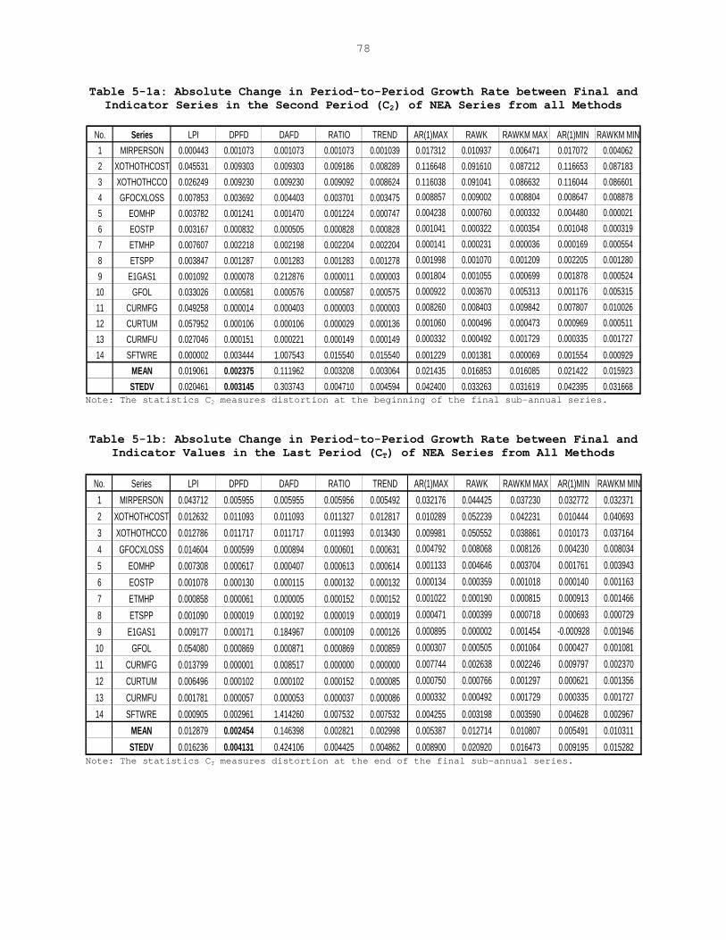
78

Table 5-1a: Absolute Change in Period-to-Period Growth Rate between Final and Indicator Series in the Second Period (C2) of NEA Series from all Methods

No. Series LPI DPFD DAFD RATIO TREND AR(1)MAX RAWK RAWKM MAX AR(1)MIN RAWKM MIN1 MIRPERSON 0.000443 0.001073 0.001073 0.001073 0.001039 0.017312 0.010937 0.006471 0.017072 0.0040622 XOTHOTHCOST 0.045531 0.009303 0.009303 0.009186 0.008289 0.116648 0.091610 0.087212 0.116653 0.0871833 XOTHOTHCCO 0.026249 0.009230 0.009230 0.009092 0.008624 0.116038 0.091041 0.086632 0.116044 0.0866014 GFOCXLOSS 0.007853 0.003692 0.004403 0.003701 0.003475 0.008857 0.009002 0.008804 0.008647 0.0088785 EOMHP 0.003782 0.001241 0.001470 0.001224 0.000747 0.004238 0.000760 0.000332 0.004480 0.0000216 EOSTP 0.003167 0.000832 0.000505 0.000828 0.000828 0.001041 0.000322 0.000354 0.001048 0.0003197 ETMHP 0.007607 0.002218 0.002198 0.002204 0.002204 0.000141 0.000231 0.000036 0.000169 0.0005548 ETSPP 0.003847 0.001287 0.001283 0.001283 0.001278 0.001998 0.001070 0.001209 0.002205 0.0012809 E1GAS1 0.001092 0.000078 0.212876 0.000011 0.000003 0.001804 0.001055 0.000699 0.001878 0.000524

10 GFOL 0.033026 0.000581 0.000576 0.000587 0.000575 0.000922 0.003670 0.005313 0.001176 0.00531511 CURMFG 0.049258 0.000014 0.000403 0.000003 0.000003 0.008260 0.008403 0.009842 0.007807 0.01002612 CURTUM 0.057952 0.000106 0.000106 0.000029 0.000136 0.001060 0.000496 0.000473 0.000969 0.00051113 CURMFU 0.027046 0.000151 0.000221 0.000149 0.000149 0.000332 0.000492 0.001729 0.000335 0.00172714 SFTWRE 0.000002 0.003444 1.007543 0.015540 0.015540 0.001229 0.001381 0.000069 0.001554 0.000929

MEAN 0.019061 0.002375 0.111962 0.003208 0.003064 0.021435 0.016853 0.016085 0.021422 0.015923STEDV 0.020461 0.003145 0.303743 0.004710 0.004594 0.042400 0.033263 0.031619 0.042395 0.031668

Note: The statistics C2 measures distortion at the beginning of the final sub-annual series.

Table 5-1b: Absolute Change in Period-to-Period Growth Rate between Final and Indicator Values in the Last Period (CT) of NEA Series from All Methods

No. Series LPI DPFD DAFD RATIO TREND AR(1)MAX RAWK RAWKM MAX AR(1)MIN RAWKM MIN1 MIRPERSON 0.043712 0.005955 0.005955 0.005956 0.005492 0.032176 0.044425 0.037230 0.032772 0.0323712 XOTHOTHCOST 0.012632 0.011093 0.011093 0.011327 0.012817 0.010289 0.052239 0.042231 0.010444 0.0406933 XOTHOTHCCO 0.012786 0.011717 0.011717 0.011993 0.013430 0.009981 0.050552 0.038861 0.010173 0.0371644 GFOCXLOSS 0.014604 0.000599 0.000894 0.000601 0.000631 0.004792 0.008068 0.008126 0.004230 0.0080345 EOMHP 0.007308 0.000617 0.000407 0.000613 0.000614 0.001133 0.004646 0.003704 0.001761 0.0039436 EOSTP 0.001078 0.000130 0.000115 0.000132 0.000132 0.000134 0.000359 0.001018 0.000140 0.0011637 ETMHP 0.000858 0.000061 0.000005 0.000152 0.000152 0.001022 0.000190 0.000815 0.000913 0.0014668 ETSPP 0.001090 0.000019 0.000192 0.000019 0.000019 0.000471 0.000399 0.000718 0.000693 0.0007299 E1GAS1 0.009177 0.000171 0.184967 0.000109 0.000126 0.000895 0.000002 0.001454 -0.000928 0.001946

10 GFOL 0.054080 0.000869 0.000871 0.000869 0.000859 0.000307 0.000505 0.001064 0.000427 0.00108111 CURMFG 0.013799 0.000001 0.008517 0.000000 0.000000 0.007744 0.002638 0.002246 0.009797 0.00237012 CURTUM 0.006496 0.000102 0.000102 0.000152 0.000085 0.000750 0.000766 0.001297 0.000621 0.00135613 CURMFU 0.001781 0.000057 0.000053 0.000037 0.000086 0.000332 0.000492 0.001729 0.000335 0.00172714 SFTWRE 0.000905 0.002961 1.414260 0.007532 0.007532 0.004255 0.003198 0.003590 0.004628 0.002967

MEAN 0.012879 0.002454 0.146398 0.002821 0.002998 0.005387 0.012714 0.010807 0.005491 0.010311STEDV 0.016236 0.004131 0.424106 0.004425 0.004862 0.008900 0.020920 0.016473 0.009195 0.015282

Note: The statistics CT measures distortion at the end of the final sub-annual series.

79

Table 5-2a: Absolute Change in Period-to-Period Growth Rate between Final and Indicator Values in the Second Period (C2) of Taxes and Transfer Payments

No. Series LPI DPFD RATIO TREND No. Series LPI DPFD RATIO TREND1 TPCAG 0.018493 0.009110 0.008296 0.008305 17 TRCAG 0.031642 0.007879 0.007591 0.0075912 TPCMI 0.072552 0.010632 0.010337 0.010510 18 TRCMI 0.029310 0.004831 0.004924 0.0049273 TPCUT 0.002654 0.002573 0.002400 0.002365 19 TRCUT 0.029292 0.005503 0.005590 0.0055954 TPCAE 0.012119 0.001877 0.002002 0.001971 20 TRCAE 0.022738 0.010853 0.011757 0.0117575 TPCCO 0.008943 0.005186 0.006252 0.005979 21 TRCCO 0.016262 0.009734 0.009696 0.0096966 TPCDG 0.008943 0.000145 0.000502 0.000502 22 TRCDG 0.025447 0.011808 0.011704 0.0125687 TPCED 0.011180 0.000902 0.001524 0.001524 23 TRCED 0.028500 0.011293 0.011294 0.0117228 TPCFR 0.007507 0.000319 0.000302 0.000296 24 TRCFR 0.023732 0.003871 0.003902 0.0037039 TPCIN 0.014039 0.000513 0.000380 0.000380 25 TRCIN 0.015417 0.007985 0.008165 0.007409

10 TPCNG 0.022426 0.002826 0.002664 0.002582 26 TRCNG 0.121623 0.040431 0.060572 0.04070311 TPCOS 0.012504 0.000835 0.001127 0.001127 27 TRCOS 0.019182 0.010779 0.011391 0.01139112 TPCPF 0.019175 0.002064 0.002330 0.002211 28 TRCPF 0.019182 0.007345 0.007353 0.00734813 TPCRT 0.011990 0.000821 0.000855 0.000821 29 TRCRT 0.026207 0.011188 0.010822 0.01134414 TPCTW 0.017095 0.011550 0.011888 0.011775 30 TRCTW 0.028514 0.008688 0.008476 0.00947115 TPCWT 0.002261 0.000292 0.000262 0.000262 31 TRCWT 0.024032 0.010570 0.009975 0.01066716 TPCGV 0.129279 0.030823 0.030470 0.030647

MEAN 0.023198 0.005029 0.005100 0.005079 MEAN 0.030739 0.010851 0.012214 0.011059STEDV 0.032526 0.007860 0.007727 0.007773 STEDV 0.025625 0.008557 0.013615 0.008649

Note: The statistics C2 measures distortion at the beginning of the final sub-annual series. LPI estimates are from 2000 to 2004 and estimates from other methods are from 1997 to 2004. Table 5-2b: Absolute Change in Period-to-Period Growth Rate between Final and

Indicator Values in the Last Period (CT) of Taxes and Transfer Payments

No. Series LPI DPFD RATIO TREND No. Series LPI DPFD RATIO TREND1 TPCAG 0.010793 0.001024 0.001899 0.001899 17 TRCAG 0.009570 0.005301 0.001394 0.0050492 TPCMI 0.012411 0.001644 0.001232 0.001174 18 TRCMI 0.013677 0.004520 0.004478 0.0034203 TPCUT 0.000366 0.000668 0.000842 0.000791 19 TRCUT 0.012528 0.004429 0.004047 0.0031934 TPCAE 0.001566 0.000328 0.000230 0.000190 20 TRCAE 0.007930 0.003557 0.002308 0.0032215 TPCCO 0.003585 0.003445 0.002725 0.002579 21 TRCCO 0.006229 0.003172 0.003003 0.0029346 TPCDG 0.002355 0.000610 0.000205 0.000205 22 TRCDG 0.005519 0.003129 0.003178 0.0023727 TPCED 0.001004 0.000183 0.000371 0.000371 23 TRCED 0.004393 0.003063 0.002927 0.0023458 TPCFR 0.002443 0.000359 0.000347 0.000343 24 TRCFR 0.026826 0.022630 0.022577 0.0138939 TPCIN 0.004657 0.001246 0.001383 0.001359 25 TRCIN 0.001812 0.003684 0.004256 0.00332010 TPCNG 0.001705 0.001062 0.001272 0.001208 26 TRCNG 0.008472 0.004066 0.004085 0.00319111 TPCOS 0.001722 0.000700 0.000472 0.000366 27 TRCOS 0.006256 0.003355 0.002964 0.00061012 TPCPF 0.002068 0.000313 0.000055 0.000055 28 TRCPF 0.003099 0.003303 0.003419 0.00255613 TPCRT 0.002064 0.000202 0.000172 0.000172 29 TRCRT 0.005842 0.003085 0.002958 0.00196514 TPCTW 0.004204 0.002021 0.001716 0.001716 30 TRCTW 0.003715 0.003657 0.003694 0.00237215 TPCWT 0.004416 0.000441 0.000467 0.000467 31 TRCWT 0.006607 0.003163 0.002574 0.00166316 TPCGV 0.011953 0.035845 0.001698 0.001820

MEAN 0.004207 0.003131 0.000943 0.000920 MEAN 0.008165 0.004941 0.004524 0.003474STEDV 0.003928 0.008765 0.000784 0.000775 STEDV 0.006106 0.004936 0.005060 0.003046

Note: The statistics CT measures distortion at the end of the final sub-annual series.

80

Table 6-1: Absolute Change in Period-to-Period Growth Rate between the Final and Indicator Values in the Linking Period (CL) Using Linking Alternative 1:

Setting Linking As An Initial Condition in the Optimization Model

Alternative 1: Linking to Benchmarked Series Linking to Benchmarked Series Obtained Using the Same Method Obtained Using LPI

Series DPFD** RATIO** TREND** DPFD* RATIO* TREND*

MIRPERSON 0.019145 0.019975 0.019144 0.029351 0.028715 0.029350

XOTHOTHCCO 0.101260 0.101252 0.108766 0.124225 0.124217 0.134156

XOTHOTHCOST 0.103711 0.103699 0.111862 0.133326 0.133320 0.145946

GFOCXLOSS 0.005340 0.005327 0.005389 0.003868 0.003868 0.003906

GFOL 0.006112 0.006102 0.006065 0.023099 0.023099 0.023506

EOMHP 0.011240 0.011241 0.011500 0.011225 0.011226 0.011225

EOSTP 0.001217 0.001304 0.001304 0.001373 0.001380 0.001380

ETMHP 0.007767 0.007776 0.006539 0.005021 0.005014 0.005014

ETSPP 0.005756 0.005756 0.005756 0.005249 0.005249 0.005249

MEAN 0.029061 0.029159 0.030703 0.037415 0.037343 0.039970 Note: ** stands for linking to benchmarked sub-annual values estimated using the same method, and * stands for linking to benchmarked sub-annual values estimated using the LPI procedure. Table 6-2: Absolute Change in Period-to-Period Growth Rate between the Final and Indicator Values in the Linking Period (CL) Using Linking Alternative 2: Replacing Previous Estimates with Revised Final Estimates in the Whole Sample

Alternative 2: Linking to Benchmarked Series Linking to Benchmarked Series Obtained Using the Same Method Obtained Using LPI

Series DPFD^ RATIO^ TREND^ DPFD RATIO TREND

MIRPERSON 0.015850 0.015851 0.017117 0.033120 0.033121 0.033187

XOTHOTHCCO 0.096004 0.095995 0.106978 0.138122 0.138113 0.143138

XOTHOTHCOST 0.098423 0.098405 0.110324 0.152860 0.152852 0.158419

GFOCXLOSS 0.006296 0.006271 0.006336 0.003744 0.003742 0.003807

GFOL 0.006747 0.006731 0.006701 0.043753 0.043751 0.043780

EOMHP 0.025510 0.025503 0.025254 0.025449 0.025439 0.024142

EOSTP 0.003523 0.003836 0.003836 0.004163 0.004145 0.004145

ETMHP 0.049781 0.049899 0.044998 0.038944 0.039000 0.039172

ETSPP 0.017140 0.017142 0.017133 0.015085 0.015086 0.015078MEAN 0.035475 0.035515 0.037631 0.050582 0.050583 0.051652

Note: ^ stands for using newly revised final estimates to replace previous estimates estimated using the same method.

81

Table 7-1: Contemporaneous Discrepancy in Two-Stage Estimation for Taxes

Stage 1=LPI Stage 2=DPFD Stage 1=DPFD Stage 2=DPFD Stage 1=RATIO Stage 2=DPFD Stage 1=TREND Stage 2=DPFDDate Diff Diff % Diff Diff % Diff Diff % Diff Diff % Diff Diff % Diff Diff % Diff Diff % Diff Diff %

1/1/1997 NA NA NA NA -66.66 0.0112 0.45 0.0000 -0.11 0.0000 0.02 0.0000 -47.22 0.0079 0.03 0.00004/1/1997 NA NA NA NA -4.25 0.0007 4.02 0.0000 -1.44 0.0002 -0.01 0.0000 -28.41 0.0047 0.07 0.00007/1/1997 NA NA NA NA 31.71 0.0051 0.91 0.0000 0.27 0.0000 -0.08 0.0000 15.20 0.0025 0.11 0.000010/1/1997 NA NA NA NA 39.21 0.0063 -1.28 0.0000 1.28 0.0002 0.17 0.0000 60.43 0.0097 0.15 0.00001/1/1998 NA NA NA NA 16.80 0.0027 -4.52 0.0000 -1.74 0.0003 0.44 0.0001 67.92 0.0108 0.19 0.00004/1/1998 NA NA NA NA 1.04 0.0002 5.94 0.0000 0.39 0.0001 0.42 0.0001 16.60 0.0026 0.24 0.00007/1/1998 NA NA NA NA -7.96 0.0012 10.68 0.0000 0.61 0.0001 0.38 0.0001 -36.21 0.0056 0.28 0.000010/1/1998 NA NA NA NA -9.85 0.0015 -13.02 0.0000 0.74 0.0001 0.56 0.0001 -48.30 0.0074 0.32 0.00001/1/1999 NA NA NA NA -4.29 0.0007 4.87 0.0000 -1.60 0.0002 0.37 0.0001 -4.55 0.0007 0.37 0.00014/1/1999 NA NA NA NA -0.30 0.0000 -18.88 0.0000 -0.10 0.0000 0.03 0.0000 -11.27 0.0017 0.44 0.00017/1/1999 NA NA NA NA 1.99 0.0003 4.28 0.0000 1.83 0.0003 -0.68 -0.0001 -6.91 0.0010 0.51 0.000110/1/1999 NA NA NA NA 2.57 0.0004 3.23 0.0000 -0.13 0.0000 0.41 0.0001 22.73 0.0033 0.57 0.00011/1/2000 7192.00 1.0310 1.96 0.0000 1.21 0.0002 3.43 0.0000 -0.28 0.0000 1.28 0.0002 55.85 0.0080 0.66 0.00014/1/2000 343.00 0.0485 4.20 0.0000 0.18 0.0000 1.01 0.0000 -0.32 0.0000 0.12 0.0000 9.86 0.0014 0.78 0.00017/1/2000 -3422.00 0.4805 6.58 0.0000 -0.50 0.0001 4.02 0.0000 -0.16 0.0000 0.14 0.0000 -29.75 0.0042 0.88 0.000110/1/2000 -4113.00 0.5723 9.12 0.0000 -0.89 0.0001 -5.81 0.0000 0.75 0.0001 0.02 0.0000 -35.96 0.0050 1.00 0.00011/1/2001 -1721.00 0.2373 11.37 0.0000 -0.88 0.0001 -10.20 0.0000 0.35 0.0000 0.11 0.0000 -4.08 0.0006 1.13 0.00024/1/2001 -78.00 0.0107 13.21 0.0000 -0.52 0.0001 -25.36 0.0000 -0.22 0.0000 -0.53 -0.0001 -23.32 0.0032 1.25 0.00027/1/2001 821.00 0.1132 14.75 0.0000 0.19 0.0000 14.36 0.0000 1.47 0.0002 1.31 0.0002 -13.91 0.0019 1.36 0.000210/1/2001 978.00 0.1326 16.15 0.0000 1.25 0.0002 -6.84 0.0000 -1.61 0.0002 0.28 0.0000 41.32 0.0056 1.41 0.00021/1/2002 324.00 0.0434 17.24 0.0000 2.76 0.0004 -11.96 0.0000 1.16 0.0002 0.12 0.0000 122.90 0.0165 1.47 0.00024/1/2002 -65.00 0.0086 21.55 0.0000 2.27 0.0003 14.98 0.0000 0.93 0.0001 0.08 0.0000 28.07 0.0037 1.57 0.00027/1/2002 -259.00 0.0336 23.83 0.0000 -0.19 0.0000 8.07 0.0000 -0.12 0.0000 0.87 0.0001 -69.49 0.0090 1.67 0.000210/1/2002 0.00 0.0000 23.68 0.0000 -4.82 0.0006 -7.34 0.0000 -1.97 0.0003 -1.13 -0.0001 -81.48 0.0105 1.76 0.00021/1/2003 120.00 0.0153 25.45 0.0000 -11.64 0.0015 -42.07 -0.0001 -1.37 0.0002 1.75 0.0002 3.43 0.0004 1.83 0.00024/1/2003 68.00 0.0086 28.21 0.0000 -9.98 0.0013 -4.19 0.0000 1.11 0.0001 0.61 0.0001 17.11 0.0022 1.93 0.00027/1/2003 -32.00 0.0040 32.96 0.0000 0.68 0.0001 -32.99 0.0000 -1.22 0.0002 -0.05 0.0000 -3.13 0.0004 2.01 0.000210/1/2003 -156.00 0.0190 35.58 0.0000 20.96 0.0026 -17.05 0.0000 1.48 0.0002 -0.04 0.0000 -17.41 0.0021 2.09 0.00031/1/2004 -845.00 0.1009 38.66 0.0000 51.65 0.0062 -10.29 0.0000 1.12 0.0001 0.78 0.0001 -4.80 0.0006 2.14 0.00034/1/2004 -591.00 0.0697 40.09 0.0000 44.20 0.0052 -22.88 0.0000 -1.84 0.0002 -0.50 -0.0001 0.18 0.0000 2.14 0.00037/1/2004 123.00 0.0144 40.74 0.0000 -3.22 0.0004 -11.31 0.0000 0.05 0.0000 -0.16 0.0000 1.01 0.0001 2.16 0.000310/1/2004 1313.00 0.1508 41.78 0.0000 -92.62 0.0106 1.64 0.0000 0.67 0.0001 -0.54 -0.0001 3.62 0.0004 2.19 0.0003

Mean 0.00 0.1547 22.35 0.0000 0.00 0.0019 -5.13 0.0000 0.00 0.0001 0.20 0.0000 0.00 0.0042 1.08 0.0001Std dev 2153.22 0.2589 12.83 0.0000 26.28 0.0030 13.20 0.0000 1.10 0.0001 0.59 0.0001 40.97 0.0040 0.76 0.0001

Table 7-2: Contemporaneous Discrepancy in Two-Stage Estimation for Transfers

Stage 1=LPI Stage 2=DPFD Stage 1=DPFD Stage 2=DPFD Stage 1=RATIO Stage 2=DPFD Stage 1=TREND Stage 2=DPFDDate Diff Diff % Diff Diff % Diff Diff % Diff Diff % Diff Diff % Diff Diff % Diff Diff % Diff Diff %

1/1/1997 NA NA NA NA -3.05 0.0109 0.00 0.0000 0.00 0.0000 0.00 0.0000 -149.00 0.5337 0.00 0.00004/1/1997 NA NA NA NA -0.29 0.0010 0.00 0.0000 1.00 0.0035 0.00 0.0000 -88.00 0.3110 0.00 0.00007/1/1997 NA NA NA NA 1.60 0.0049 0.00 0.0000 -2.00 0.0061 0.00 0.0000 0.00 0.0000 0.00 0.000010/1/1997 NA NA NA NA 1.72 0.0058 0.00 0.0000 1.00 0.0034 0.00 0.0000 237.00 0.8050 0.00 0.00001/1/1998 NA NA NA NA 0.86 0.0027 0.00 0.0000 0.00 0.0000 0.00 0.0000 317.00 1.0000 0.00 0.00004/1/1998 NA NA NA NA 0.13 0.0004 0.00 0.0000 -1.00 0.0032 0.00 0.0000 130.00 0.4208 0.00 0.00007/1/1998 NA NA NA NA -0.34 0.0010 0.00 0.0000 0.00 0.0000 0.00 0.0000 -127.00 0.3884 0.00 0.000010/1/1998 NA NA NA NA -0.65 0.0015 0.00 0.0000 1.00 0.0022 0.00 0.0000 -320.00 0.7169 0.00 0.00001/1/1999 NA NA NA NA -0.22 0.0006 0.00 0.0000 -1.00 0.0029 0.00 0.0000 -7.00 0.0200 0.00 0.00004/1/1999 NA NA NA NA -0.02 0.0001 0.00 0.0000 0.00 0.0000 0.00 0.0000 -51.00 0.1447 0.00 0.00007/1/1999 NA NA NA NA 0.09 0.0003 0.00 0.0000 -1.00 0.0028 0.00 0.0000 -28.00 0.0783 0.00 0.000010/1/1999 NA NA NA NA 0.13 0.0003 0.00 0.0000 2.00 0.0053 0.00 0.0000 86.00 0.2281 0.00 0.00001/1/2000 752.00 1.7735 0.00 0.0000 0.07 0.0002 0.00 0.0000 0.00 0.0000 0.00 0.0000 200.00 0.4717 0.00 0.00004/1/2000 36.00 0.0834 0.00 0.0000 0.01 0.0000 0.00 0.0000 0.00 0.0000 0.00 0.0000 75.00 0.1738 0.00 0.00007/1/2000 -357.00 0.8122 0.00 0.0000 -0.04 0.0001 0.00 0.0000 0.00 0.0000 0.00 0.0000 -114.00 0.2594 0.00 0.000010/1/2000 -431.00 0.9527 0.00 0.0000 -0.06 0.0001 0.00 0.0000 0.00 0.0000 0.00 0.0000 -161.00 0.3559 0.00 0.00001/1/2001 -179.00 0.3865 0.00 0.0000 -0.05 0.0001 0.00 0.0000 -1.00 0.0022 0.00 0.0000 26.00 0.0561 0.00 0.00004/1/2001 -8.00 0.0170 0.00 0.0000 -0.02 0.0000 0.00 0.0000 2.00 0.0043 0.00 0.0000 23.00 0.0490 0.00 0.00007/1/2001 86.00 0.1733 0.00 0.0000 0.02 0.0000 0.00 0.0000 1.00 0.0020 0.00 0.0000 -24.00 0.0484 0.00 0.000010/1/2001 101.00 0.2136 0.00 0.0000 0.07 0.0001 0.00 0.0000 -2.00 0.0042 0.00 0.0000 -25.00 0.0529 0.00 0.00001/1/2002 34.00 0.0727 0.00 0.0000 0.18 0.0004 0.00 0.0000 -2.00 0.0043 0.00 0.0000 26.00 0.0556 0.00 0.00004/1/2002 -6.00 0.0129 0.00 0.0000 0.13 0.0003 0.00 0.0000 0.00 0.0000 0.00 0.0000 12.00 0.0258 0.00 0.00007/1/2002 -29.00 0.0622 0.00 0.0000 -0.01 0.0000 0.00 0.0000 2.00 0.0043 0.00 0.0000 -15.00 0.0322 0.00 0.000010/1/2002 1.00 0.0021 0.00 0.0000 -0.28 0.0006 0.00 0.0000 0.00 0.0000 0.00 0.0000 -23.00 0.0493 0.00 0.00001/1/2003 30.00 0.0631 0.00 0.0000 -0.67 0.0014 0.00 0.0000 0.00 0.0000 0.00 0.0000 -19.00 0.0400 0.00 0.00004/1/2003 16.00 0.0330 0.00 0.0000 -0.58 0.0012 0.00 0.0000 0.00 0.0000 0.00 0.0000 -16.00 0.0330 0.00 0.00007/1/2003 -8.00 0.0162 0.00 0.0000 0.05 0.0001 0.00 0.0000 1.00 0.0020 0.00 0.0000 2.00 0.0040 0.00 0.000010/1/2003 -38.00 0.0760 0.00 0.0000 1.19 0.0024 0.00 0.0000 -1.00 0.0020 0.00 0.0000 33.00 0.0660 0.00 0.00001/1/2004 -191.00 0.3719 0.00 0.0000 2.98 0.0058 0.00 0.0000 0.00 0.0000 0.00 0.0000 59.00 0.1149 0.00 0.00004/1/2004 -134.00 0.2571 0.00 0.0000 2.55 0.0049 0.00 0.0000 -1.00 0.0019 0.00 0.0000 24.00 0.0461 0.00 0.00007/1/2004 23.00 0.0481 0.00 0.0000 -0.19 0.0004 0.00 0.0000 1.00 0.0021 0.00 0.0000 -26.00 0.0544 0.00 0.000010/1/2004 302.00 0.5518 0.00 0.0000 -5.38 0.0098 0.00 0.0000 0.00 0.0000 0.00 0.0000 -57.00 0.1042 0.00 0.0000

Mean 0.00 0.2990 0.00 0.0000 0.00 0.0018 0.00 0.0000 0.00 0.0018 0.00 0.0000 0.00 0.2106 0.00 0.0000Std dev 238.48 0.4406 0.00 0.0000 1.43 0.0028 0.00 0.0000 1.08 0.0019 0.00 0.0000 117.92 0.2560 0.00 0.0000

Note: LPI estimates are from 2000 to 2004 and estimates from other methods are from 1997 to 2004.

82

Table 8-1a: Average Absolute Period-to-Period Growth Rates of 10 Nonnegative Series with (with no Indicators)

No Series LPI DAFD BFLFD BFLSD RATIO

1 CGNTRMVGM 0.023405 0.021686 0.021686 0.022544 0.021698

2 CGNTRD 0.022476 0.018115 0.018115 0.019001 0.018124

3 CGNTRWC 0.012288 0.011966 0.011966 0.012215 0.011964

4 CGNTRMVCHP 0.147960 0.152658 0.153884 0.136917 0.153983

5 IBT811 0.070604 0.061159 0.061159 0.065522 0.061168

6 SUB230 0.008720 0.007409 0.007407 0.007485 0.007364

7 SUB270 0.021909 0.017439 0.017439 0.017856 0.017534

8 SUB420 0.196998 0.170361 0.172380 0.178834 0.169732

9 SUB370 0.084699 0.078003 0.078002 0.082908 0.078017

10 CUROTHPOW 0.039285 0.019513 0.019513 0.021267 0.019513MEAN 0.062834 0.055831 0.056155 0.056455 0.055910STEDV 0.063841 0.060243 0.060889 0.059506 0.060345

Table 8-1b: Average Absolute Period-to-Period Change in Level of 5 Series

with Negative Values (with no Indicators) No Series LPI DAFD BFLFD BFLSD RATIO11 ENT210 1.276596 1.032340 1.032843 1.115596 NA12 ENT230 30.446809 31.502340 31.502088 33.923819 NA13 ENT260 1.000000 0.680000 0.684605 2.539333 NA14 ENT330 6.680851 6.362979 6.362781 6.788759 NA15 ENT390 84.454545 83.853636 83.852493 86.886250 NA

MEAN 24.771760 24.686259 24.686962 26.250751 NASTEDV 35.49169395 35.42170396 35.42037586 36.42909631 NA

Table 8-2a: Period-to-Period Growth Rate in the Second and Last Periods for

10 Nonnegative Series (with no indicators) Perod-to-period growth rate in second period Period-to-period growth rate in period T

No Series LPI DAFD BFLFD BFLSD RATIO LPI DAFD BFLFD BFLSD RATIO

1 CGNTRMVGM 0.032407 0.008242 0.008234 0.033392 0.008301 0.009831 0.001589 0.001594 0.001853 0.001581

2 CGNTRD 0.076803 0.004719 0.004727 0.015832 0.004689 0.053591 0.010363 0.010368 0.039420 0.010215

3 CGNTRWC 0.010700 0.002202 0.002208 0.005663 0.002197 0.006607 0.002997 0.003004 0.009008 0.002891

4 CGNTRMVCHP 0.980769 0.855564 0.867715 0.705519 0.872928 0.031250 0.008663 0.008668 0.028051 0.008653

5 IBT811 0.016692 0.006208 0.006200 0.051918 0.006024 0.044795 0.005834 0.005828 0.053421 0.005511

6 SUB230 0.000000 0.002712 0.002688 0.006793 0.000000 0.000000 0.000258 0.000267 0.001478 0.000000

7 SUB270 0.022989 0.003803 0.003750 0.005436 0.011236 0.015000 0.006155 0.006165 0.020230 0.005000

8 SUB420 0.044118 0.013564 0.013675 0.061061 0.013699 0.130081 0.058041 0.058059 0.229874 0.061728

9 SUB370 0.054217 0.012591 0.012593 0.064276 0.011457 0.026087 0.000289 0.000289 0.032888 0.000000

10 CUROTHPOW 0.020180 0.002322 0.002331 0.025108 0.002331 0.000241 0.000269 0.000278 0.004725 0.000278MEAN 0.125887 0.091193 0.092412 0.097500 0.093286 0.031748 0.009446 0.009452 0.042095 0.009586STEDV 0.301219 0.268604 0.272445 0.214827 0.273975 0.039076 0.017457 0.017461 0.068245 0.018670

Table 8-2b: Period-to-Period Change in Level in the Second and Last Period

for 5 Series with Negative Values (with no indicators) Perod-to-period level change in second period Period-to-period level change in period T

No Series LPI DAFD BFLFD BFLSD RATIO LPI DAFD BFLFD BFLSD RATIO11 ENT210 7.000000 0.390000 0.392000 1.950306 NA 0.000000 0.380000 0.379384 1.381385 NA12 ENT230 21.000000 11.250000 11.242637 33.943410 NA 2.000000 1.750000 1.750832 1.334403 NA13 ENT260 1.000000 1.490000 1.489087 5.028955 NA 1.000000 0.680000 0.684605 2.539333 NA14 ENT330 10.000000 0.740000 0.744938 3.643498 NA 10.000000 5.090000 5.094136 18.364176 NA15 ENT390 3.000000 12.050000 12.051963 52.603882 NA 23.000000 8.850000 8.849186 34.293185 NA

MEAN 8.400000 5.184000 5.184125 19.434010 NA 7.200000 3.350000 3.351629 11.582496 NASTEDV 7.861298 5.922743 5.920239 22.766691 NA 9.679876 3.598173 3.597543 14.599927 NA

83

Table 9-1: Comparative Evaluation of the Methods Used in the Estimation of the 14 NEA Series According to the Test Criteria

Mean of Statistics LPI DPFD DPAD RATIO TREND AR(1)MAX RAWK RAWKM MAX AR(1)MIN RAWKM MIN

DXp 0.979053 1.000000 1.000000 1.000000 1.000000 1.000000 1.000000 1.000000 1.000000 1.000000

Cp 0.027965 0.013470 0.874160 0.013768 0.014024 0.017374 0.022031 0.024061 0.016992 0.023555

CB 0.009378 0.015853 0.473065 0.016138 0.016837 0.019595 0.025468 0.027999 0.019633 0.027988

C2 0.019061 0.002375 0.111962 0.003208 0.003064 0.021435 0.016853 0.016085 0.021422 0.015923

CT 0.012879 0.002454 0.146398 0.002821 0.002998 0.005387 0.012714 0.010807 0.005491 0.010311

CL NA 0.029061 NA 0.029159 0.030703 NA NA NA NA NA Note: Each entry contains the mean of the test statistics of the 14 series from a particular method used in estimation. Table 9-2: Comparative Evaluation of the Methods Used in Estimation of Series

on Taxes and Transfer Payments According to the Test Criteria

16 series of taxes on production and imports 15 series of transfer payments

Mean of Statistics LPI DPFD RATIO TREND LPI DPFD RATIO TREND

DXp 1.000000 1.000000 1.000000 1.000000 1.000000 1.000000 1.000000 1.000000

Cp 0.008395 0.008836 0.008982 0.008856 0.014911 0.018859 0.018866 0.018728

CB 0.005212 0.010446 0.010460 0.010527 0.009545 0.022080 0.022137 0.022186

C2 0.023198 0.005029 0.005100 0.005079 0.030739 0.010851 0.012214 0.011059

CT 0.004207 0.003131 0.000943 0.000920 0.008165 0.004941 0.004524 0.003474

DXC(%) 0.154714 0.024831 0.024834 0.024855 0.296904 0.001800 0.001835 0.000397

Note: Each entry in the left panel contains the mean of the test statistics of the 16 series on taxes from a particular method used in estimation, and each entry in the right panel contains the corresponding mean statistics of the 15 series on transfer payments. Estimates from LPI are from 2000 to 1997 and estimates from other methods are from 1997 to 2004. Table 9-3: Comparative Evaluation of the Methods Used in Estimation of Series

without Sub-annual Indicators According to the Test Criteria

Average statistics for 10 non-negative series Average statistics for 5 series with negative values

Mean of Statistics LPI DAFD BFLFD BFLSD RATIO LPI DAFD BFLFD BFLSD RATIO

gt 6.283447 5.583084 5.615520 5.645487 5.590992 24.771760 24.686259 24.686962 26.250751 NA

g2 12.588737 9.119256 9.241199 9.749978 9.328617 8.400000 5.184000 5.184125 19.434010 NA

gT 3.174829 0.944566 0.945199 4.209480 0.958577 7.200000 3.350000 3.351629 11.582496 NA Note: Each entry in the left panel contains the mean of the test statistics of the 10 nonnegative series without indicators, and each entry in the right panel contains the corresponding test statistics of the 5 series with negative values.

84

Appendix: Information on Series and Software Used in the Experiment

Table A1: Series Used in Estimation Experiment

Series

Definition

Series with Indicators 1 MIRPERSON.a

JTOTN.q Monetary Interest Paid by Persons

2 XOTHOTHCOST.A MTGVALORIG.Q

Total Closing Cost Mortgage Originations, seasonally adjusted

3 XOTHOTHCCO.A MTGVALORIG.Q

Owner-Occupied Closing Cost Mortgage Originations, seasonally adjusted

4 GFOCXLOSS$.A JGFOCXLOSS$.Q

Crop Output Constant-Dollar Gross Crop Output Excluding Losses

5 EOMHP EOMH

Owner-Occupied Mobile Homes Extrapolated using Mobile Home Housing Stock

6 EOSTP EOST

Owner-Occupied Stationary Homes Extrapolated using Stationary Unit Housing Stock

7 ETMHP ETMH

Tennant-Occupied Mobile Homes Extrapolated using Mobile Home Housing Stock

8 ETSPP ETSP

Tennant-Occupied Stationary Homes Extrapolated using Stationary Unit Housing Stock

9 E1GAS1.A E1GAS0A.M

Consumption of Gasoline Monthly Indicator of Gasoline Consumption

10 GFOL$.A JGFOL$.Q

Livestock output Constant-Dollar Gross Livestock Output

11 CURMFG.A VIPMFG.M

Nonresidential Manufacturing Monthly Value Estimates for Nonresidential Const.

12 CURTUM.A VIPTCM.M

Nonresidential Telecommunications Monthly Value Estimates for Telecommunications Const.

13 CURMFU.A VIPMFU.M

Residential Multi-Family Monthly Value Estimates for Multi-Family Const.

14 SFTWRE QIND_PRE_SA.Q

Investment in Pre-Packaged Equipment & Software Quarterly Indicator

15 TPCAG TPCTL

Taxes on Ag., Forestry, Fishing, Hunting Total Taxes

16 TPCMI TPCTL

Taxes on Mining Total Taxes

17 TPCUT TPCTL

Taxes on Utilities Total Taxes

18 TPCAE TPCTL

Taxes on Arts, Entertainment, etc. Total Taxes

19 TPCCO TPCTL

Taxes on Construction Total Taxes

20 TPCDG TPCTL

Taxes on Durable Goods Total Taxes

21 TPCED TPCTL

Taxes on Education, Health, Social Assistance Total Taxes

22 TPCFR TPCTL

Taxes on Fin., Ins., Real Est., Rental, Leasing Total Taxes

23 TPCIN TPCTL

Taxes on Information Total Taxes

24 TPCNG TPCTL

Taxes on Nondurable Goods Total Taxes

25 TPCOS TPCTL

Taxes on Other Services, Except Government Total Taxes

26 TPCPF TPCTL

Taxes on Professional & Business Services Total Taxes

27 TPCRT TPCTL

Taxes on Retail Trade Total Taxes

28 TPCTW TPCTL

Taxes on Transportation & Warehousing Total Taxes

29 TPCWT TPCTL

Taxes on Wholesale Trade Total Taxes

30 TPCGV TPCTL

Taxes on Government Enterprises Total Taxes

31 TRCAG TRCTL

Transfers from Ag., Forestry, Fishing, Hunting Total Transfers

32 TRCMI TRCTL

Transfers from Mining Total Transfers

85

Table A1: Series Used in Estimation Experiment (Cont.)

Series

Definition

Series with Indicators 33 TRCUT

TRCTL Transfers from Utilities Total Transfers

34 TRCAE TRCTL

Transfers from Arts, Entertainment, etc. Total Transfers

35 TRCCO TRCTL

Transfers from Construction Total Transfers

36 TRCDG TRCTL

Transfers from Durable Goods Total Transfers

37 TRCED TRCTL

Transfers from Education, Health & Social Assistance Total Transfers

38 TRCFR TRCTL

Transfers from Fin., Ins., Real Est., Rental, Leasing Total Transfers

39 TRCIN TRCTL

Transfers from Information Total Transfers

40 TRCNG TRCTL

Transfers from Nondurable Goods Total Transfers

41 TRCOS TRCTL

Transfers from Other Services, Except Government Total Transfers

42 TRCPF TRCTL

Transfers from Professional & Business Services Total Transfers

43 TRCRT TRCTL

Transfers from Retail Trade Total Transfers

44 TRCTW TRCTL

Transfers from Transportation & Warehousing Total Transfers

45 TRCWT TRCTL

Transfers from Wholesale Trade Total Transfers

Series without Indicators

46 CGNTRMVGM

State & Local Transfers: General Medical Assistance

47 CGNTRTD

TDI Benefits

48 CGNTRWC Workers Compensation Benefits

49 CGNTRMVCHP State & Local Transfers: Child Health Program

50 ENT210

OPIC

51 ENT230

Bonneville Power

52 ENT260

Colorado River Basins

53 ENT370

TVA

54 ENT390

National Flood Insurance

55 IBT811

Outer Continental Shelf Royalties

56 SUB230

Housing-235-236-Rent Supplement

57 SUB270

Rental Assistance

58

SUB310 Amtrak

59 SUB420

Maritime Operating

60 CUROTHPOW.A

Nonresidential Other Power

Note: The indictors and their definitions are in italic letters. TPC-series: Taxes on production & imports. TRC-series: Business transfers to government. ENT-series: Current surplus of government enterprise. SUB-series: Subsidies. IBT-series: Indirect business Taxes.