Municipality disaggregation of German's agricultural...

Copyright 2011 by Norbert Röder and Alexander Gocht. All rights reserved. Readers may make verbatim copies of this document for non-commercial purposes by any means, provided that this copyright notice appears on all such copies.

Paper prepared for the 122nd EAAE Seminar

"EVIDENCE-BASED AGRICULTURAL AND RURAL POLICY MAKIN G: METHODOLOGICAL AND EMPIRICAL CHALLENGES OF POLICY

EVALUATION" Ancona, February 17-18, 2011

Municipality disaggregation of German's agricultural sector

model Raumis

Röder N.1 and Gocht A.1

1 Johann Heinrich von Thünen-Institute; Institute of Rural Studies, Bundesallee 50, 38116 Braunschweig, Germany

[email protected]

Ancona - 122nd EAAE Seminar "Evidence-Based Agricultural and Rural Policy Making”

Page 1 of 14

Municipality disaggregation of German's agricultural sector

model Raumis

Röder N. and Gocht A.

Abstract Since several decades the RAUMIS modelling system is applied for policy impact assessments to measure the impact of agriculture on the environment. A disaggregation at the municipality level with more than 9.000 administrative units, instead of currently used 316 counties, would tremendously improve the environmental impact analysis. Two sets of data are used for this purpose. The first are geo-referenced data, that are, however, incomplete with respect its coverage of production activities in agriculture. The second set is the micro census statistic itself, that has a full coverage, but data protection rules (DPR) prohibit its straightforward use. The paper show how this bottleneck can be passed to obtain a reliable modelling data set at municipality level with a complete coverage of the agricultural sector in Germany. We successfully applied a Bayesian estimator, that uses prior information derived a cluster analysis based on the micro census and GIS information. Our test statistics of the estimation, calculated by the statistical office, comparing our estimates and the real protected data, reveals that the proposed approach adequately estimates most activities and can be used to fed the municipality layer in the RAUMIS modelling system for an extended policy analysis. Keywords: Highest Posterior Density estimator (HPD), RAUMIS, Down scaling JEL classification: C11, C61, C81, Q15.

1. INTRODUCTION

Frequently, the impact of agricultural activities on the environment can only be properly

assessed if the underlying distribution is well-covered. For instance, the likely impact of new

pests such as the western corn rootworm (Diabrotica virgifera ssp. virgifera LeConte), which is

relevant to the debate on bT-maize, depends on the share of maize in the crop rotation. Namely,

if the share of maize exceeds 50%, western corn rootworm may have a serious impact

(CARRASCO et al., 2009). If we analyse the cultivated area in 2007 at the county level (316

regions in Germany) the results indicate that the cultivation of maize in Germany should barely

be affected by the rootworm (FDZ, 2010). However, if we conduct the same analysis on the

municipality level, almost 13% of the maize cultivating areas would be affected by the

rootworm. Thus, because agricultural land use and its dynamics are site-dependent, the

utilisation of wider regional averages to model specific situations can be misleading (e.g.,

OSTERBURG et al., 2009, p. 40 ff.).

The agricultural and environmental modelling and information system RAUMIS

(HENRICHSMEYER et al., 1996) is a mathematical programming, modelling and information

platform used to cover Germany’s agricultural sector. RAUMIS is used to analyse agricultural

and agri-environmental policy instruments and currently operates at the county level. Similar to

other economic models such as CAPRI (BRITZ and WITZKE, 2008), the RAUMIS model


Page 2 of 14

simulates an aggregate over all farms in a particular region. To overcome problems related to

data aggregation, the underlying heterogeneity of farming patterns must be represented. Thus,

several different approaches have been applied to disaggregate regional models. For example, a

specifically tailored component in the CAPRI model has been used to disaggregate crop shares,

stocking densities and fertilizer application rates from about 250 administrative regions across

Europe into clusters of 1x1 km grid cells (LEIP et al., 2008) that are based on homogeneous

spatial mapping units (KEMPEN et al., 2005). Other downscaling approaches of agricultural

statistical data with the help of geographical and/or remote sensing data are presented by

DENDONCKER et al., (2006), VERBURG et al. (2006), YOU and WOOD, (2006). However, the

resulting resolution with respect to animal and crop categories is very limited and therefore less

useful in modelling agricultural decision process. Also if the results are spatially disaggregated

into clusters of grid cells, the borders of the clusters do not necessarily coincide with

administrative boundaries. Alternatively, a disaggregation of regional production levels into

farming groups such as done by GOCHT and BRITZ (2010) is an option. However, this approach

also has serious disadvantages because of the missing territorial representation which in turn

does not allow spatially geo-referenced data to be linked, an important feature for regional

models as RAUMIS.

Alternatively and in the focus of this study, county data are disaggregated to the

municipality level using Agricultural Census data and GIS data. However, the provision of data

is limited by legal constraints. In particular, many production activities at the municipality level

fall under the data protection regulation (DPR) and are not reportable because the number of

observations is limited. Currently, the DPR is by censoring data if they are derived from less

than three observations or if a one or two observations dominate the result (primary

confidentiality) (EUROSTAT, 2009). In Germany a result is viewed as being dominated if a

single observation contributes more than 80% to the aggregate (FDZ, personal communication).

Furthermore, additional aggregates are censored to ensure that data censored in step one cannot

be retrieved from the published data (secondary confidentiality). As result, the likelihood that

the data will be censored increases with increasing resolution.

If we want to overcome this and disaggregate the county data for the RAUMIS model to

the municipality level using Agricultural Census data we need a method to extract additional

information from official statistical offices without violating DPR. In contrast to GOCHT and

ROEDER (2010) who apply a method based on locally weighted averages and only restricted to a

specific region in Germany, we propose an algorithm that recovers local information with the

help of the activities’ median at the municipality level German wide. These medians are

calculated for clusters of similar municipalities. The aim of the present study is to develop an

algorithm that is capable to depict the distribution of agricultural land use with the spatial

resolution of municipalities. We evaluate the estimated results with respect to both relative

intensities (i.e. shares in the crop rotation and stocking levels) and absolute values (i.e. ha or

livestock units (LU)). To our knowledge no attempt has been made so far at this coverage and


Page 3 of 14

administrative resolution, which results in a public and not traceable dataset for policy impact

assessment.

The remainder of the paper is organized as follows. Section 2 highlights some key

characteristics of the data. In Section 3, we describe the applied data manipulation algorithms

and introduce the estimation framework. Lastly, Section 4 presents the results, and we conclude

in a final section.

2. METHODS

The section starts with explaining the preparatory steps necessary to overcome

inconsistent data definitions between the statistical data bases and the RAUMIS model

definition, before we describe the estimation framework and we finalize introducing the test

statistic used to evaluate our estimates.

Figure 1 presenting the consecutive processing steps in order to facilitate the

understanding of the data processing and handling. It distinguishes between two data processing

environments. Processing at the Research data centre (FDZ) is done via sending data

processing algorithm of standard statistical packages to the FDZ and because a researcher has

never direct access to the micro data, one is forced to construct the processing algorithm

virtually blind, knowing only the data structure and definition of the data. These conditions are

rather uncomfortable because a validation whether a result is an observed trend or just a

phenomena resulting from mapping or definition errors is difficult. Also the situation that

economic simulation models are rarely realized in a standard statistical package makes the

direct processing in the FDZ environment very cumbersome, and often impossible for economic

policy evaluation. However, the big advantage is to have the opportunity to use the high

resolution micro data shown in Figure 1 with the AFiD-Panel Agriculture database, to derive

indicators. The Panel provides extensive information on the agricultural activities of farms in a

four year interval for all farms in Germany.

All routines to be processed at the FDZ will be checked and results leave the FDZ only

when they are in compliance with the DPR, presented in Figure 1 as the dotted rectangle

between the two processing environments. Figure 1 also shows the processing at office

environment, which is the researcher's office. Here we can use the outcome of the FDZ, which

is anonymous not traceable and in compliance with the DPR for further analysis and

applications. In Figure 1 step 3 illustrates the setup of an estimation framework, in which we

use GIS data together with the FDZ information to obtain a consistent municipality data set.

We now explain step 1 until 3 in more detail: The data preparation in Step 1 comprise the

usual preparatory data work, mainly harmonizing definitions. As we need for RAUMIS a

consistent data set at municipality level for several years from 1999 onwards we had to adjust

and map regional definitions. As example, municipalities merged, split or exchanged and hence

significant amounts of land. After harmonizing we remained with 9,679 time consistent

municipality units. We had to aggregate some statistical codes to be in line with our 36

RAUMIS agricultural production activities.


Page 4 of 14

Figure 1: Information flow in the estimation procedure

A) Consistent municipality data set

B) Data set with test statistics

1) Data preparation

4) Calculate test statistics

3) Estimate consistent municipality data set

Farm Structure Survey Microdata(FDZ 1999, 2003, 2007)

GIS land use data(BKG, 2008)

Control of Compliance with data protection regulations

Processing at FDZ

Processing at Office

2) Calculate Municipality clusters

Country aggregates for activities(FDZ, 2010)

Source: Own elaboration

As the DPR prevent a direct retrieval of RAUMIS production activities at municipality

level, we developed in Step 2 a processing algorithm that complies with the DPR. We clustered

the 9,679 regional units into 180 clusters based on several indicators for general land use, arable

land use and animal density given in Table 1. For the three groups we independently applied the

kMeans-algorithm (Witten & Frank, 2005). The algorithm was sent to the FDZ and applied to

the micro data.

Table 1: Indicators obtained from each cluster Indicator group Unit Indicators

General land use % of utilized agricultural area (UAA) Arable land, cereals, root crops, vegetables, main forage area, fruits, grassland, rough pastures

Arable land use % of arable land

winter wheat, summer barley, rye, other winter cereals, other cereals, grain maize, rape seed, potatoes, sugar beet, green maize, other forage crops on arable land, other crops, set aside

Livestock husbandry Livestock units (LU) per ha of UAA Suckler cows, dairy cows, heifers, bulls, calves, sheep, horses, poultry, pig fattening, pig breeding

Source: Own elaboration

For each cluster, and hence the municipalities belonging to it, we obtained median and

standard deviation of the respective indicators from the FDZ. In Step 3 we setup an estimation

framework with the aim to estimate the municipality production structure of our 36 RAUMIS


Page 5 of 14

production activities. We setup the model per county. Hence we have to solve 316 models. With

each model we estimate the maximum 36 possible production activities for all municipalities in

a county the number of municipalities per county ranges from 6 to 159 with a median of 25. In

addition, the estimation algorithm uses GIS information on the extent of five land use types

(utilized agricultural area (UAA), arable land, grassland, wine yards and orchards) and the

agricultural production statistic at the country level, which is public available.

The cluster median for each indicators is interpreted as a priori information in the

Bayesian sense, whereas the data information consists of the given county production values,

sum of production activities over the municipalities is equal to the county level, and the

constraint that the estimated activity levels add up to observed land use type, observed in GIS

data GOCHT and ROEDER (2010).

Our Bayesian Highest Posterior Density estimator (HPD) maximizes the log of the joint

posterior density (see HECKELEI et al., 2008), i.e. it searches for the most probable deviations

from the cluster median fitting our data information on country activity level and the land type

GIS information. Without knowledge about the exact distribution of the error terms in the

clustered data, normally distributed errors with a co-variance of zero between the different

medians and the obtained variance from FDZ are assumed.

The constraints alone do not allow a unique solution to be identified because there are too

many unknown vectors of estimated cropping hectares and livestock herd sizes, exceeding the

number of data constraints from GIS and country level statistic. Therefore, prior information

must be included in combination with a penalty function. Generalised maximum entropy

(GOLAN et al., 1996) has frequently been applied to this end. However, we used the HPD

estimation, which allows a direct and transparent formulation of prior information and reduces

the computational complexity of the model (HECKELEI ET AL., 2008).

After we applied the estimation we obtained absolute and relative shares for all RAUMIS

activities. In Step 4, we calculate test-statistics to verify our findings by comparing the obtained

estimates with the micro census data. We had to use the virtually blind approach, sending the

estimates together with the routines to the FDZ and obtained the test statistics. We evaluated the

distribution of the differences between estimated and observed cropping shares and livestock

densities weighted with the respective local production level to assess the overall quality of the

results.

The following software was used for the analysis at the FDZ: SAS 9.1 for regression and

cluster analysis and the Conopt3-solver in GAMS 23.5 for the Bayesian minimisation problem.

3. RESULTS

In section 3.1 we analyse the overall fit of the model using the weighted differences

between observed and estimated cropping shares and livestock densities. Afterwards we

compare for selected activities the real intensity gradient at municipality level with the ones

resulting from our estimation approach and a distribution obtained by a naive break down of

"county shares" using to the municipality in a county. We finish this section with a detailed


Page 6 of 14

analysis of the distribution and development of maize production in Germany to illustrate the

potential of high resolution data.

3.1. Error Distribution

Table 2 shows that for nearly all analyzed livestock activities the estimated livestock

densities deviate from the observed ones by less than 0.1 LU per ha. For cattle, sheep and horses

roughly 90% of the stock is located in municipalities where the density is estimated with an

accuracy of ± 0.1 LU per ha. The distribution of granivores is covered worse. Here, especially

for laying hens the density is partly significantly underestimated. However, this is not surprising

as especially egg and poultry production pronounced local concentrations are typical.

Table 2: Distribution of the differences between the estimated and observed livestock

densities at municipality level (in LU per ha) (differences weighted with respective local level)

Quantile of the error distribution

RAUMIS Description 5% 25% 50% 75% 95%

KALB Calves -0.11 -0.04 -0.01 0.01 0.12

BULL Male cattle > 6 month; stock bulls -0.10 -0.03 0.00 0.04 0.11

FAER Heifers -0.16 -0.02 0.01 0.04 0.11

MIKU Dairy cows -0.12 -0.02 0.01 0.04 0.10

AMMU Suckler and fattening cows -0.09 -0.03 -0.01 0.01 0.05

SCHA Sheep -0.13 -0.04 -0.02 0.00 0.04

SOTI Other livestock (horses) -0.09 -0.03 -0.01 0.01 0.05

SAUH Sows for piglet production -0.30 -0.06 -0.01 0.03 0.11

SMAS Pig fattening -0.24 -0.04 0.01 0.07 0.27

LEHE Laying hens -3.46 -0.15 -0.05 0.00 0.32

SOGE Poultry fattening (broiler, turkeys, etc.) -0.69 -0.21 -0.07 0.00 0.27 Source: FDZ, own calculation.

Also for the cropping shares the local shares are generally well met (table 3). For

cropping activities generally 50% of the production is located in municipalities where the

respective share on the UAA is estimated with accuracy above ± 3%. The algorithm hardly

overestimates the cropping share at the local level. Especially, the share of wheat, rye, rape

seed, the grassland activities, fruits, vegetable, set aside and fallow is severely underestimated in

some areas. The large differences for rape seed, set aside, and rye might be linked to their

concentration in Eastern Germany. Here, the farms are rather large in comparison to the

municipalities so the difference between the land use in the cadastre for the municipality and the

actual land use of the farms in this municipality might be rather large. For the three grassland

activities the difference might be explained by a mutual exchange of activities in particular

meadows and pastures. In addition in particular the location of the rough grazing reported in the

cadastre is likely to differ significantly from the distribution according to the Agricultural

Census as not all these areas are managed by farms or where included in the definition of

agricultural area. The last argument might also explain the problems observed in fruits,

vegetables and fallow.


Page 7 of 14

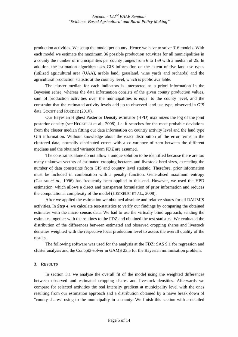
Table 3: Distribution of the differences between estimated and observed cropping shares at

municipality level (in % of UAA) (differences weighted with respective local level)

Quantile of the error distribution

RAUMIS Description 5% 25% 50% 75% 95%

WWEI Winter wheat, spelt -0.40 -0.02 0.02 0.04 0.08

SWEI Summer wheat, durum wheat -0.07 -0.02 -0.01 0.00 0.01

WGER Winter barley -0.11 -0.02 0.00 0.02 0.05

SGER Summer barley -0.06 -0.02 0.00 0.02 0.06

ROGG Rye, and winter cereal mixes -0.20 -0.03 0.00 0.04 0.10

HAFE Oats and summer cereal mixes -0.05 -0.02 -0.01 0.00 0.03

KMAI Grain maize (including CCM) -0.07 -0.03 0.00 0.03 0.11

SGET Other cereals, triticale -0.07 -0.03 -0.01 0.01 0.05

RAPS Rape and turnip rape -0.21 -0.02 0.01 0.03 0.06

HUEL Pulses -0.07 -0.03 -0.01 0.00 0.05

SHAN Other oilseeds and industrial crops (hops, tobacco, etc.)

-0.09 -0.04 -0.01 0.00 0.04

SKAR Potatoes -0.06 -0.03 -0.01 0.02 0.07

ZRUE Sugar beet -0.08 -0.02 0.00 0.02 0.05

SHAC Other root crops (fodder beet, etc.) -0.03 -0.01 0.00 0.00 0.00

SMAI Green and silage maize -0.09 -0.02 0.00 0.03 0.07

FEGR Grass on arable land (including all other fodder on arable land)

-0.09 -0.03 -0.01 0.02 0.06

WIES Meadow -0.20 -0.03 0.00 0.03 0.09

WEID Pasture -0.27 -0.08 -0.02 0.01 0.11

HUTU Rough pastures -0.19 -0.05 -0.02 0.00 0.05

FLST Set aside -0.15 -0.08 -0.06 -0.04 -0.02

GEMU Vegetables, strawberries -0.15 -0.06 -0.02 0.00 0.05

SOPF Other plant production (flowers, nurseries, etc.) -0.09 -0.02 -0.01 0.00 0.03

OBST Fruits (without strawberries) -0.16 -0.03 -0.01 0.00 0.03

REBL Wine -0.10 -0.03 0.00 0.02 0.07

FALL Fallow -0.52 -0.03 -0.01 0.00 0.01 Source: FDZ, own calculation.

3.2. Fit of the estimate

Figure 2 compares for different production activities the cumulative density distribution

observed at the municipality level (red curve = Municipality observed) with the outcome of the

estimation procedure described above (blue curve = Municipality estimated) and a distribution

calculated naively on the county shares (green curve = Municipality taken over from county

shares). Note, we do not present the tails of each curve as the extreme values of the observed

distribution at municipality levels are censored due to DPR. For a better comparability all

curves are truncated to the available interval that ranges from the 5% to 95% quantile.


Page 8 of 14

The first row presents the shares of arable land and grass land on UAA. The second row depicts

production activity shares for maize, winter wheat and sugar beet on arable land and the last row

visualizes the distribution for dairy cows, other cattle and fattening pigs. Each of the curves is a

cumulated density distribution, it depicts how much of a certain activity level (y-axes) can be

represented by a certain range of shares from zero up to the indicated share of the curve on the

x-axes.

Figure 2: Cumulated density plots for selected agricultural activities in 2007

5%

25%

45%

65%

85%

0% 20% 40% 60% 80%

Cu

mu

late

d s

ha

re o

f m

aiz

e

Share on arable land

Maize

Mun. estimated

Mun. observed

County observed

5%

25%

45%

65%

85%

0% 20% 40% 60% 80% 100%

Cu

mu

late

d s

ha

re o

f a

rab

le la

nd

Share on UAA

Arable land

5%

25%

45%

65%

85%

0% 20% 40% 60%

Cu

mu

late

d s

ha

re o

f w

inte

r w

he

at


Winter wheat

5%

25%

45%

65%

85%

0% 20% 40% 60% 80% 100%

Cu

mu

late

d s

ha

re o

f g

rass

lan

d

Share on UAA

Grassland

5%

25%

45%

65%

85%

0% 10% 20% 30%

Cu

mu

late

d s

ha

re o

f su

ga

r b

ee

t


Sugar beet

5%

25%

45%

65%

85%

0,0 0,5 1,0 1,5 2,0 2,5

Cu

mu

late

d s

ha

re o

f d

air

y c

ow

s

LU per ha UAA

Dairy cows

5%

25%

45%

65%

85%

0,0 0,5 1,0 1,5 2,0 2,5

Cu

mu

late

d s

ha

re o

f o

the

r ca

ttle

LU per ha UAA

Other cattle

5%

25%

45%

65%

85%

0,0 0,5 1,0 1,5 2,0 2,5 3,0 3,5

Cu

mu

late

d s

ha

re o

f fa

tte

nin

g p

igs

LU per ha UAA

Fattening pigs

Source: FDZ, and own calculation.

In all figures, the county shares are on the left side of the observed shares. This is not

surprising as we lose the heterogeneity of shares across municipalities by the aggregation of the

observed municipality level (red line) to county shares and their re-assignment to all

municipalities of a county. The green line presents the current resolution of the RAUMIS

modelling system, for which we assume that shares for production activities at county level

equal those in the municipalities. This does not hold as differences between county and

observed municipality exists, as presented in Figure 2.

We also can observe that the steeper the curve is for a given activity the smaller is the

heterogeneity of production shares range in which the majority of the production can be found.

As example for grassland: 45% of Germany’s total grassland is located in municipalities where


Page 9 of 14

the share of grassland on UAA is below 40% and roughly 18% of the grassland is located in

municipalities where the respective share is above 80% (red curve). If the shares are calculated

on a county base instead more than 55% of Germany’s grassland is located in counties where

the share is below 40% and roughly 10% is located in counties where the grassland share

exceeds 80% (green curve). One can see that the blue curve (the estimated values at

municipality level) follow the red (the observed distribution) quite closely. The green curve (if

county averages are taken as a proxy for the local situation) is far left of the red one. As

indicated before, this implies that in particular the proportion of grassland in areas with a

grassland share of 25% to 60% is greatly overestimated. The distribution of arable land differs

quite significantly from the one for grassland. Only 10% of Germany’s arable land is located in

counties or municipalities where the arable land accounts for less than 50% of the UAA. At

municipality level for arable land the fit between the estimated and observed distribution is

lower than for grassland. In tendency the difference between the observed distribution at

municipality level and the estimated at municipality on the one hand and the county averages is

comparable. While the county averages locate more arable land in areas with lower shares of

arable land (underestimate the specialisation). Our estimation approach is overspecialised

compared to the observed distribution at municipality level. This result might be explained by

the fact that there exists a difference of nearly 2 million ha (~ 30% of the grassland according to

the census) between the grassland areas reported in the Agricultural Census and the cadastre. If

this error is not randomly distributed a slight systematic underestimation of the grassland share

in municipalities with high shares of arable land will lead due to the large lever of the grassland

share to a significant right shift of the curve (Taking a municipality of 1,000 UAA and a share

of arable land of 10% an underestimation of 1% (= error of 10 ha grassland) will relocate 910 ha

of arable land to the right (to areas with higher shares of arable land)).The tendency to

overspecialize is found in other production activities, particular with high shares as winter

wheat. Another reason for the overspecialisation might be the fact that for most activities the

standard deviation, which we use as an indicator for the confidence we have in the

appropriateness of a cluster median for a designated municipality is strongly positively with

cluster median. This implies that larger shares are intrinsically associated with a lower

confidence in the value and a deviation from the prior information is less punished in our HPD

estimation framework.

To summarize Figure 2 the municipality based estimator outperforms the county based

approach especially for activities that are of smaller overall importance and locally concentrated

like rough grazing, sugar beet, wine, potatoes, or poultry.

3.3. Local distribution and development and cultivation of maize in Germany

After we evaluated the quality of the estimation, we will use of the obtained results to

analyse the distribution and development of maize shares in Germany at municipality levels, to

gain more insight into possible phytosanitary problems. To our knowledge, such an exercise is

done for Germany for the first time with such a resolution.


Page 10 of 14

Figure 3 depicts the estimated distribution on municipality level of maize (grain and green) in

Germany for 2007. Despite the fact that maize was grown only on 16% of Germany’s arable

land, maize covers more than 33% of the respective arable land in a couple of areas. One centre

regarding the cultivation of maize lies in north-western Germany between the Ruhrgebiet and

Rhine in the south-west and the Elbe in the north-east. Regarding the cultivation of maize a

second large hot spot is located in south-eastern Bavaria east of the Inn and between the Alps

and the Bavarian Forest. Smaller areas with high shares of maize (beyond 33%) can be found in

the Geest (Schleswig Holstein), the Upper Rhine valley (Baden-Württemberg), the foothills of

the Allgäu (Baden-Württemberg and Bavaria) and the Sauerland (Northrhine-Westphalia).

Maize reaches, hence, in several areas quite critical levels regarding phytosanitary issues when

the distribution is analysed at municipality level.

Figure 3: Dynamic of estimated maize shares on arable land 2007 compared to 1999

Source: Own estimation

In the following section we analyze the development of maize shares depicted by the

small maps in Figure 3. The area cultivated with maize expanded by 300,000 ha between 1999

and 2007 resulting in a moderate increase of maize’s share on total arable land from 13.3% to

15.9%. However, these aggregate figures cover a quite significant dynamic on the local level

that we now are able to analyze with the outcome of the estimation. In large parts of North-

Western Germany, in the Geest, and in the vicinity of mountain ranges (Eifel, Sauerland,

Allgäu, Alps and Bavarian forest) maize’s share on arable land increased by more than 10%.


Page 11 of 14

Till 2002 the cultivation of maize was strongly linked to arable forage cropping in particular

dairy farming and bull fattening. This explains the high shares of maize in areas with high cattle

densities (e.g. along the North Sea and in the foothill of the alps). Grain maize including corn-

cob mix was important in the Upper Rhine Valley, along the border between Northrhine-

Westphalia and Lower Saxony and in south east of Bavaria. While the area of grain maize

remained nearly constant over the last decade the area of green maize declined parallel to the

declining cattle stock till 2002. From 2002 till 2007 the maize area expanded by more than

360,000 ha due to the promotion of biogas production based on silage maize (BMELV, various

years). While the cultivation of maize declined in the north-western part of Northrhine

Westphalia, the eastern part of Bavaria and the northern part of Baden-Württemberg. This

development is critical for two reasons. First, maize cultivation is expanded in areas where

maize is already the dominant crop, increasing phytosanitary risks. Second, the cultivation of

maize in mountain ranges induces a high risk of erosion, as in these areas the precipitation is

high, the terrain is fairly undulated and maize is developing a protective vegetation cover late in

the year.

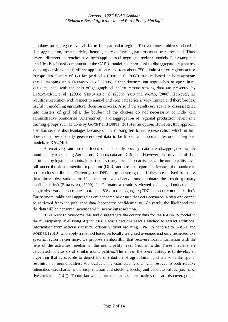
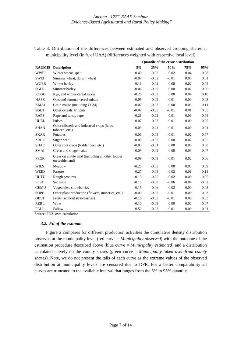
Figure 4 compares the result obtained from the estimation approach and the county

averages for the share of maize on arable land. In large parts of Germany the county averages

are a reasonable estimate for the municipality shares (e.g. Rhineland-Palatine, Hesse, Thuringia,

and Saxony). However, the county averages underestimate drastically the relevance of maize in

the Geest of Schlewig-Holstein and Lower Saxony, and in the foothills of the Alps, the Bavarian

Forst and the Odenwald. On the other hand the relevance of maize is overestimated for large

parts of the Black forest, the marsh land of Lower Saxony and the north eastern part of

Schleswig-Holstein.


Page 12 of 14

Figure 4: Difference between the estimated share of maize on arable land for 2007

(estimated municipality shares – county averages)

Source: Own estimation

4. CONCLUSIONS AND OUTLOOK

The proposed method of disaggregation, which combined the highest posterior density

(HPD) and a cluster analysis improved land use estimates at the municipality level and

complied with the data protection rules (DPR) at the FDZ.

The correlation between the observed and predicted values was analysed for the entire

data set in German, and the results indicated that the proposed approach can adequately depict

the spatial and density distribution of most RAUMIS activities while complying with the DPR.

Not surprisingly the described procedure greatly improves the mapping quality for

activities whose distribution shows are clear spatial pattern that does not coincidence with the

county borders e.g. the distribution of rough pastures or the distribution of maize in Schleswig-

Holstein and Baden-Württemberg. If an activity is widespread and dominant the advantage of

the estimated results versus a naive downscaling of the county shares is less clear.

For most activities the described procedure generally covers well the intensity gradient

present in Germany’s agriculture. However, it has slight tendency for an overspecialisation. In


Page 13 of 14

principle, there are three reasons why our estimated results on the municipality level deviate

from the observed levels:

1. The reference area and therefore the plot is not recorded in the same municipality as the

farmstead. In the FSS the UAA is attributed to a municipality according to the locality of

the farmstead, while in the cadastre the plot the situs principle is applied.

2. Agricultural used areas are wrongly recorded in the cadastre or Agricultural Census. To

illustrate the importance of this fact, one has to keep in mind that the agricultural area

reported in the cadastre exceeds the one of the FSS by nearly 2 million ha or 10%.

3. False attribution of activities on the municipality level (in step 3). This can be due to

several reasons. First, the fact that the median is not a suitable estimator for the activity

level in a given municipality. Second, the assumption of a normal error distribution is

oversimplifying. Third, the weighting of the different parts of the error term is

inappropriate.

REFERENCES

BKG (Bundesamt für Kartographie und Geodäsie) (2008): Basis-DLM (Digitales Basis-Landschaftsmodell)

1:25 000. Frankfurt / Main.

BMELV (Bundesministerium für Ernährung,. Landwirtschaft und Verbraucherschutz) (Various years): Statistisches

Jahrbuch über Ernährung, Landwirtschaft und Forsten der Bundesrepublik Deutschland.

Britz W. and Witzke, P. (2008): CAPRI model documentation (2008): Available at http://www. capri-

model.org/docs/capri_documentation.pdf, pp. 181.

Carrasco L. R., T. D. Harwood, S. Toepfer, A. MacLeod, N. Levay, J. Kiss, R. H. A. Baker, J. D. Mumford and

Knight, J. D. (2009): Dispersal kernels of the invasive alien western corn rootworm and the effectiveness of buffer

zones in eradication programmes in Europe. Annals of Applied Biology 156 (1): 63-77.

Dendoncker N., P. Bogaert, and Rounsevell, M. (2006): A statistical method to downscale aggregated land use data

and scenarios. Journal of Land Use Science 1 (2): 63-82.

EUROSTAT (2009): Statistical disclosure control. Available at:

http://epp.eurostat.ec.europa.eu/portal/page/portal/research_methodology/methodology/statistical_disclosure_control.

Last update: 25.04.2009.

FDZ (Research Data Centres of the Federal Statistical Office and the Statistical Offices of the Länder) (2010), AFID-

panel agriculture, 1999, 2003 and 2007.

Gocht A, and Britz, W. (2010), EU-wide farm types supply in CAPRI - How to consistently disaggregate sector

models into farm type models, Journal of Policy Modeling.

Gocht, A. and N. Röder (2010): Recovering localized information on agricultural structure underlying data

confidentiality regulations - potentials of different data aggregation and segregation techniques. Paper presented at

50th annual conference of the GEWISOLA "Möglichkeiten und Grenzen der wissenschaftlichen Politikanalyse",

Braunschweig, 29.09. - 01.10.2010. URL: http://purl.umn.edu/93975.

Golan A., G. Judge and Miller, D. (1996): Maximum entropy econometrics, Robust Estimation with Limited Data.

John Wiley, New York.

Heckelei T., T. Jansson, and Mittelhammer, R. (2008): A Bayesian Alternative to Generalized Cross Entropy

Solutions for Underdetermined Econometric Models Discussion Paper 2008:2, University of Bonn, Available at

http://www.ilr1.uni-bonn.de/agpo/publ/dispap/ download/dispap08_02.pdf

Henrichsmeyer, W., Cypris, C., Löhe, W., Meudt, M., Sander, R., von Sothen, F., Isermeyer, F., Schefski, A.,

Schleef, K.-H., Neander, E., Fasterding, F., Helmcke, B., Neumann, M., Nieberg, H., Manegold, D., and Meier, T.


Page 14 of 14

(1996): Entwicklung eines gesamtdeutschen Agrarsektormodells RAUMIS96. Endbericht zum Kooperationsprojekt.

Forschungsbericht für das BML (94 HS 021), 1996, vervielfältigtes Manuskript Bonn/Braunschweig.

Kempen M., Britz W. and Heckelei T. (2005): A Statitical Approach for Spatial Disaggregation of Crop Production

in the EU, In: Arfini Filippo (ed.). Modelling agricultural policies: state of the art and new challenges; proceedings of

the 89th European Seminar of the European Association of Agricultural Economists (EAAE), Parma, Italy, February

3rd-5th, 2005. Parma : Monte Universita Parma Editore, pp. 810-830.

Leip A., Marchi G., Koeble R., Kempen M., Britz W. and Li C. (2008): Linking an economic model for European

agriculture with a mechanistic model to estimate nitrogen and carbon losses from arable soils in Europe.

Biogeosciences 5(1), 73-94.

Osterburg B., H. Nitsch, B. Laggner and W. Roggendorf (2009): Auswertung von Daten des Integrierten

Verwaltungs- und Kontrollsystems zur Abschätzung von Wirkungen der EU-Agrarreform auf Umwelt und

Landschaft. Arbeitsberichte aus der vTI-Agrarökonomie 07/2009. Braunschweig.

verburg p., c. schulp, n. witte and a. veldkamp (2006): Downscaling of land use change scenarios to assess the

dynamics of European landscapes. Agriculture, ecosystems and environment 114: 39–56.

Witten, I.H. and E. Frank (2005): Data Mining: Practical Machine Learning Tools and Techniques. Elsevier.

Amsterdam

You L. and S. Wood (2006): An entropy approach to spatial disaggregation of agricultural production. Agricultural

Systems 90: 329-347.

Zellner A. (1971): An introduction to Bayesian inference in econometrics. New York: Wiley.

Municipality disaggregation of German's agricultural...

Documents

Transcript of Municipality disaggregation of German's agricultural...