Unsupervised Disaggregation of Low Frequency Power Measurements

Hyungsul Kim∗ Manish Marwah† Martin Arlitt† Geoff Lyon† Jiawei Han∗

AbstractFear of increasing prices and concern about climate changeare motivating residential power conservation efforts. Weinvestigate the effectiveness of several unsupervised disag-gregation methods on low frequency power measurementscollected in real homes. Specifically, we consider variantsof the factorial hidden Markov model. Our results indi-cate that a conditional factorial hidden semi-Markov model,which integrates additional features related to when andhow appliances are used in the home and more accuratelyrepresents the power use of individual appliances, outper-forms the other unsupervised disaggregation methods. Ourresults show that unsupervised techniques can provide per-appliance power usage information in a non-invasive manner,which is ideal for enabling power conservation efforts.

1 Introduction

Concern over global climate change has motivated ef-forts to reduce the emissions of CO2 and other GHGs(greenhouse gases). Energy use in the residential sectoris a significant contributor of GHGs [49]. For example,the residential sector is responsible for over one third ofall electricity use in the United States [2]. While infor-mation is available on the typical use of electricity inhomes (e.g., space heating, space cooling, water heat-ing and lighting account for about 50% of all residentialelectricity use [3]), it has not enabled most home ownersto reduce their electricity consumption.

Two typical approaches to conserving energy are ef-ficiency and curtailment [1]. The former involves one-time actions (e.g., upgrading to more energy-efficientappliances) that have a higher cost. The latter re-quires continuous participation (e.g., using less heat-ing/cooling on a daily basis), with a smaller incremen-tal cost. There are two general issues that inhibit con-sumers from applying these techniques. First, energyuse is a very abstract concept to most consumers [24, 8].Second, consumers are often mistaken about how en-ergy is used in the home, and thus which actions wouldbe most beneficial for conserving energy [15, 4, 38].Numerous studies have identified the attributes of asolution to these issues: personalized, frequent, con-tinuous, credible, clear and concise feedback that pro-vides an appliance-specific breakdown of how energy isused in the home [5, 19, 7, 1, 11, 13, 15, 38]. Fieldstudies showed that with proper feedback, residential

∗University of Illinois, Urbana-Champaign, IL†HP Labs, Palo Alto, CA

electricity and/or gas use could be reduced by up to50% [14], although typical savings were in the 9%-20%range [42, 20, 45, 1, 47]. Improved feedback can alsohelp curtail peak use by up to 50% [27, 44].

Much of this research occurred decades ago, in re-sponse to the oil crisis in the 1970s [39]. At that time,computer hardware technology was not as advanced, soproviding frequent feedback to home owners cost effec-tively seemed infeasible [19]. As the crisis subsided(and prices dropped), the financial incentive to con-serve diminished [45]. The growing concern over climatechange has revived the importance of conservation. To-day, computer hardware technology is more advanced,so frequent feedback is now feasible. In particular, asold power meters are replaced with smart meters, moreinformation will be available to consumers [38].

An open issue is how to provide an appliance-specific breakdown of energy use in a cost-effectivemanner. Without this, residential energy conservationefforts are unlikely to achieve widespread success. Thispaper investigates how to obtain this information viapower load disaggregation. While this topic has receivedattention since the early 1990s [18], our work has threedistinguishing characteristics. First, we assume only lowfrequency measurements are available. This makes ourtechniques more widely applicable since smart meterstypically provide samples no more than once per second.Second, we use an unsupervised disaggregation approach,as this does not require the data to be labeled, which canbe laborious and intrusive. Third, we use empirical datacollected from seven homes over a six month period.

The specific problem we address is as follows. Giventhe aggregate power consumption for T time periods,Y = 〈y1, y2, . . . , yT 〉, and the number of appliances,M , we want to infer the power load of each of the Mappliances, that is,

Q(1) = 〈q(1)1 , q(1)2 , . . . , q

(1)T 〉

Q(2) = 〈q(2)1 , q(2)2 , . . . , q

(2)T 〉

...

Q(M) = 〈q(M)1 , q

(M)2 , . . . , q

(M)T 〉

such that yt =∑Mi=1 q

(i)t , where q

(i)t is the power load

of appliance i at time t.We achieve this using energy disaggregation meth-

747 Copyright © SIAM.Unauthorized reproduction of this article is prohibited.

ods based on extensions of a hidden Markov model(HMM). We use four HMM variants to model the data.Factorial HMM (FHMM) models the hidden states ofall the appliances. Conditional FHMM (CFHMM) ex-tends FHMM to incorporate additional features, suchas time of day, other sensor measurements, and depen-dency between appliances. A third variant, factorialhidden semi-Markov model (FHSMM) extends FHMMto better fit the probability distributions of the state oc-cupancy durations of the appliances. The fourth variantcomposes FHSMM and CFHMM, to consider the addi-tional features together with the more accurate proba-bility distributions of the state occupancy durations ofthe appliances. We refer to this variant as conditionalfactorial hidden semi-Markov model (CFHSMM).

Our paper makes two key contributions. First, weexplore four unsupervised techniques for disaggregatinglow frequency power load data. Second, we provide aperformance evaluation of the techniques using powerload data from real homes. We find that CFHSMMoutperforms the other variants, and demonstrate thatunsupervised disaggregation techniques are feasible.

The remainder of the paper is organized as follows.Section 2 provides background information and relatedwork. Section 3 discusses features that can be used fordisaggregation of low frequency power measurements.Section 4 describes the four models we use to identifythe stable-state signatures of household appliances. Sec-tion 5 presents our results, using power load data fromactual homes. Section 6 summarizes our work.

2 Background and Related Work

2.1 Background Hidden Markov Models (HMM)are used for probabilistically modeling sequential data.HMMs are known to perform well at tasks such asspeech recognition [37], problems in computational bi-ology [28], etc.

A discrete-time hidden Markov model can be viewedas a Markov model whose states are not directly ob-served: instead, each state is characterized by a prob-ability distribution function, modeling the observationscorresponding to that state. More formally, an HMM isdefined by the following:

– S = {S1, S2, · · · , SN} the finite set of hidden states.

– the transition matrix A = {aij , 1 ≤ i, j ≤ N}representing the probability of moving from stateSi to state Sj ,

aij = P (qt+1 = Sj |qt = Si), 1 ≤ i, j ≤ N,

with aij ≥ 0,∑Nj=1 aij = 1, and where qt denotes

the state occupied by the system at time t.

P(d1=2)

ON ON OFF ON

ON ON ON OFF

ON ON OFF OFF

yt-1 yt yt+1 yt+2

OFF

OFF

ON

yt-2y

q3

q2

q1

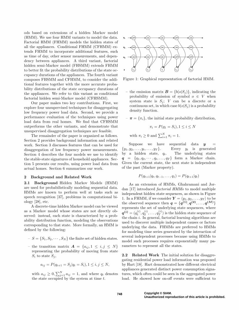
Figure 1: Graphical representation of factorial HMM.

– the emission matrix B = {b(o|Sj)}, indicating theprobability of emission of symbol o ∈ V whensystem state is Sj ; V can be a discrete or acontinuous set, in which case b(o|Sj) is a probabilitydensity function.

– π = {πi}, the initial state probability distribution,

πi = P (q1 = Si), 1 ≤ i ≤ N

with πi ≥ 0 and∑Ni=1 πi = 1.

Suppose we have sequential data y ={y1, y2, . . . , yt, . . . , yT }. Every yt is generatedby a hidden state, qt. The underlying statesq = {q1, q2, · · · , qt, . . . , qT } form a Markov chain.Given the current state, the next state is independentof the past (Markov property).

P (qt+1|qt, qt−1, . . . , q1) = P (qt+1|qt)

As an extension of HMMs, Ghahramani and Jor-dan [17] introduced factorial HMMs to model multipleindependent hidden state sequences, as shown in Figure1. In a FHMM, if we consider Y = 〈y1, y2, . . . , yT 〉 to bethe observed sequence then q = {q(1), q(2), . . . , q(M)}represents the set of underlying state sequences, where

q(i) = (q(i)1 , q

(i)2 , . . . , q

(i)T ) is the hidden state sequence of

the chain i. In general, factorial learning algorithms areused to discover multiple independent causes or factorsunderlying the data. FHMMs are preferred to HMMsfor modeling time series generated by the interaction ofseveral independent processes because using HMMs tomodel such processes requires exponentially many pa-rameters to represent all the states.

2.2 Related Work The initial solution for disaggre-gating residential power load information was proposedby Hart [18]. Hart demonstrated how different electricalappliances generated distinct power consumption signa-tures, which often could be seen in the aggregated powerload. He showed how on-off events were sufficient to

748 Copyright © SIAM.Unauthorized reproduction of this article is prohibited.

characterize the use of some appliances. For other ap-pliances, Hart considered using Finite State Machinesto develop signatures. Hart called this approach “Non-intrusive Appliance Load Monitoring”(NALM).

Other research efforts have attempted to improveNALM, often by proposing alternative signature identi-fication techniques. Farinaccio and Zmeureanu [12] usea pattern recognition approach to disaggregate whole-house electricity consumption into its major end-uses.Prudenzi [36] proposes a neural net approach for identi-fying the electrical signatures of residential appliances.Laughman et al. suggest collecting data at higher fre-quencies (e.g., 8,000 Hz) to use higher harmonics in theaggregate current signal to generate appliance signa-tures [29]. Ito et al. [22] extract features from the cur-rent (e.g., amplitude, form, timing) to develop appliancesignatures. Suzuki et al. [46] use an integer program-ming approach to disaggregate residential power use.Saitoh et al. [41] extract nine features from the mea-sured current signal, and use them to classify the state ofan appliance. Kato et al. [23] describe an “electric appli-ance recognition method”. It uses Principal ComponentAnalysis (PCA) to extract features from electric signals.These features are classified using a Support Vector Ma-chine. For “unregistered” appliances, a one-class SVMis used. Lin et al. [31] use a dynamic Bayesian networkto take user behavior into account, and a Bayes filter todisaggregate the data online. However, these methodshave practical limitations which motivate the develop-ment of alternative techniques. Matthews et al. reflecton some of these works and describe the characteristicsof a workable solution [32]. Our work focuses specificallyon disaggregating low frequency power load data with-out the need for extra sensors, as these are importantattributes of a cost-effective solution.

Several research efforts have prototyped tools forin-home use. Serra et al. built a prototype power me-ter, which included software to disaggregate the powerconsumption and automatically identify different ap-pliances (as well as to detect malfunctioning appli-ances) [43]. However, they considered only a small num-ber of appliances and used very simple signatures; thusthe approach seems unsuitable for actual home environ-ments. Kim et al. augment electricity usage data froma single power meter with ambient signals from inexpen-sive sensors placed near appliances [25]. They use threetypes of indirect sensors: magnetic, acoustic and light,to distinguish between multiple appliances that are si-multaneously on and monitor variable power consump-tion. Unfortunately, the need for additional sensors isundesirable from a practical perspective.

An interesting variation on the NALM approachwas proposed by Patel et al. [35]. They use a plug-in

sensor to detect electrical events within a home. Theyleverage the fact that mechanical switches produce elec-trical noise [21], and that the noise characteristics canvary dramatically by appliance [48]. They apply ma-chine learning techniques to recognize specific devicesbeing turned on or off. More specifically, they performa Fast Fourier Transform on the incoming signal to sep-arate the component frequencies. They then use a Sup-port Vector Machine to classify which appliance wasturned on. In several trials, they found accuracies of85–90% in classifying the events. However, they cannotdetermine the power consumed during each event fromthe noise. To address this, they developed a sensor thatcan be installed by the end user [34].

Disaggregating power data in commercial settingshas additional challenges. For example, Norford andLeeb [33] present results for space-conditioning equip-ment in an commercial setting. Some of the challengesinclude more identical appliances, and more complexappliance signatures.

Lastly, hidden Markov models have been appliedto a wide range of topics. One relevant study isfrom Yadwadkar et al. [50]. They use profile hiddenMarkov models to recognize distinct applications withina network file trace. The success of their approachmotivates us to explore HMMs for developing appliancesignatures for residential power use.

3 Disaggregation with Low Sampling Rates

There are two kinds of features for power disaggregation– transient signatures and stable-state signatures [18].Transient signatures capture electrical events, such ashigh frequency noise in electrical current or voltage,generated as a result of an appliance turning on oroff [35]. Although these features are good candidatesfor use in disaggregation, sampling data fast enoughto capture them requires special instrumentation. Forexample, Patel et al. use a custom built device tomeasure at rates up to 100KHz [35]. However, mostsmart meters deployed in the U.S. have low samplingrates, typically 1Hz or less.

Stable-state signatures relate to more sustainedchanges in power characteristics when an appliance isturned on/off. These persist until the state of theappliance changes, which can be captured with lowfrequency sampling. But even for stable-state features,the frequency of sampling is important since at lowsampling rates the probability of multiple on/off eventsoccurring between two measurements increases, makingthe disaggregation task more difficult. In addition tothe real power measurement, AC power meters typicallyprovide several other metrics, such as, reactive power,frequency, power factor, etc., each of which could

749 Copyright © SIAM.Unauthorized reproduction of this article is prohibited.

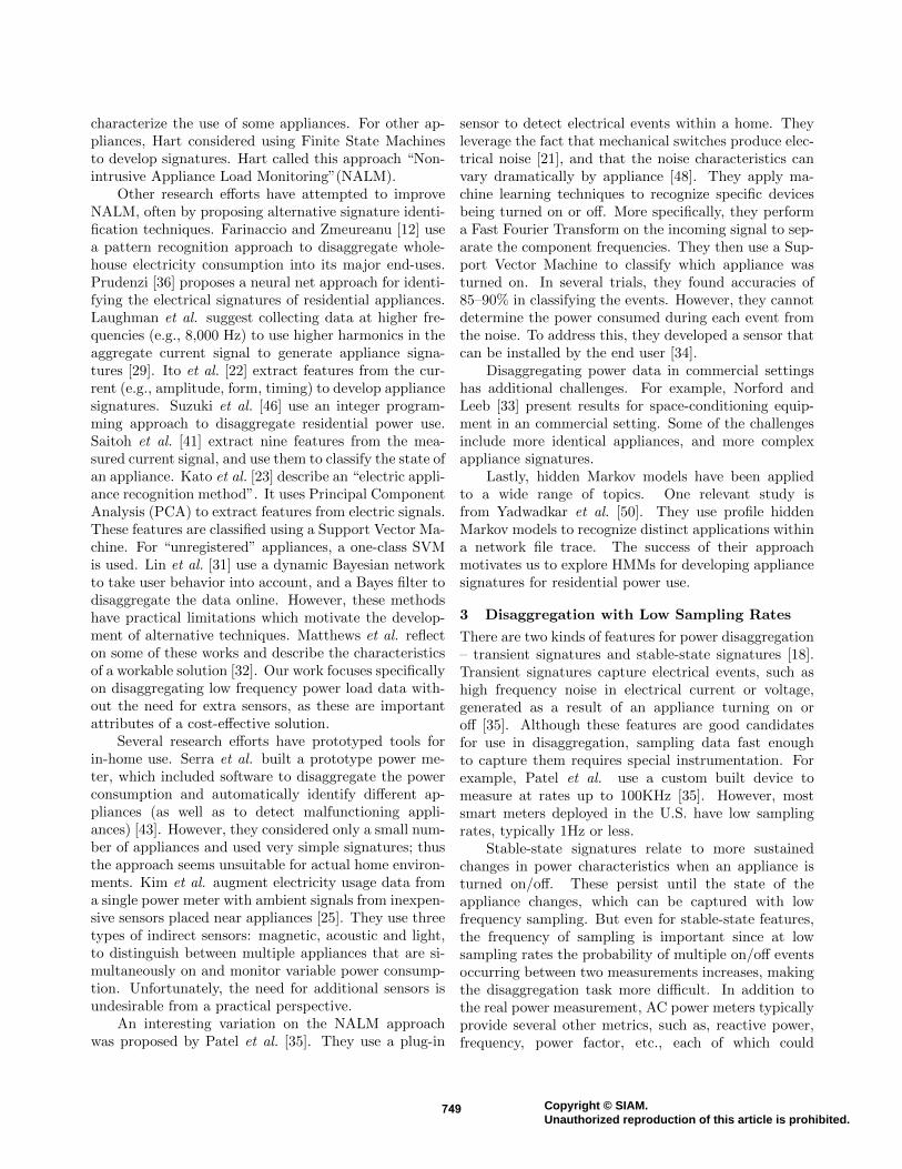
Label Location Appliance Powerfam tv Family Room Television 73 Wfam ps3 Family Room Playstation 3 67 Wfam stereo Family Room Home Theater 41 Wkit ref Kitchen Refrigerator 82 Wliv tv Living Room Television 177 Wliv xbox Living Room Xbox 360 111 Woff laptop Office Laptop 61 Woff monitor Office Monitor 38 W

Table 1: Summary of the household appliances.

potentially be used as additional features depending onthe set of appliances to be disaggregated.

In this work, we focus on stable-state featuressince these features can be more readily obtained,e.g., from smart meters, in which case no additionalinstrumentation is required in the homes. The mosteffective feature for disaggregation is the real powermeasurement. However, other power features may helpdistinguish appliances, so our approach is designedto allow multiple other features to be integrated intothe model. Other useful features, unrelated to powermetrics, are: duration on/off, date/time, dependencybetween appliances, daily schedule of the occupants,etc. Further, unlike past work, we develop unsupervisedlearning algorithms for disaggregating the appliances.

We collected detailed power measurements from 7homes in California, for a period of six months. To en-able us to know the ground truth, we installed extensiveinstrumentation in the home, collecting data at the indi-vidual appliance level. We then aggregate the data frommultiple individual appliances to test the ability of themethods to disaggregate this data. We use the originaltraces of power use for each instrumented appliance toassess the performance of the disaggregation methods.It is important to clarify that if we can successfully dis-aggregate the aggregate power data, thorough (and ex-pensive) instrumentation of homes will not be necessaryto obtain per-appliance measurements. Further, labo-rious ”labelling” of the collected data is not required.This is an important practical consideration, and themotivation for our focus on unsupervised techniques.

In the following subsections, we focus on one home,and investigate the possible stable-state features. Ta-ble 1 lists a subset of the monitored appliances in thehome. Each “Label” is an abbreviation formed from theappliance type and its location. For example, “fam tv”is the television located in the Family Room, while“liv tv” is the television located in the Living Room.

3.1 Power Consumption The real power consump-tion is the most significant feature. Table 1 shows theaverage values for each of the appliances. We assumethat each appliance has two states (on and off) and

fam_tv

Watt

Fre

qu

en

cy

0

5000

10000

15000

20000

25000

0 50 100 150 200 250

fam_ps3

Watt

Fre

qu

en

cy

0

200

400

600

800

1000

1200

0 50 100 150 200 250

fam_stereo

Watt

Fre

qu

en

cy

0

5000

10000

15000

20000

0 50 100 150 200 250

kit_ref

Watt

Fre

qu

en

cy

0

5000

10000

15000

20000

25000

0 50 100 150 200 250

liv_tv

Watt

Fre

qu

en

cy

0

500

1000

1500

2000

2500

3000

3500

0 50 100 150 200 250

liv_xbox

Watt

Fre

qu

en

cy

0

500

1000

1500

0 50 100 150 200 250

off_laptop

Watt

Fre

qu

en

cy

0

500

1000

1500

2000

2500

3000

0 50 100 150 200 250

off_monitor

Watt

Fre

qu

en

cy

0

10000

20000

30000

40000

50000

60000

0 50 100 150 200 250

Figure 2: Histograms of appliance power consumption.

fam_tv

Duration in Minutes

Fre

quen

cy

0

20

40

60

80

100

120

0 50 100 150 200 250 300

fam_ps3

Duration in Minutes

Fre

quen

cy

0

5

10

15

20

25

30

0 50 100 150 200 250 300

fam_stereo

Duration in Minutes

Fre

quen

cy

0

10

20

30

40

50

60

70

0 200 400 600 800

kit_ref

Duration in Minutes

Fre

quen

cy

0

500

1000

1500

2000

2500

3000

3500

0 20 40 60 80 100

liv_tv

Duration in Minutes

Fre

quen

cy

0

20

40

60

80

100

0 50 100 150 200 250 300

liv_xbox

Duration in Minutes

Fre

quen

cy

0

10

20

30

40

50

60

0 50 100 150 200 250 300

off_laptop

Duration in Minutes

Fre

quen

cy

0

50

100

150

200

0 50 100 150 200 250 300

off_monitor

Duration in Minutes

Fre

quen

cy

0

10

20

30

40

0 2000 4000 6000 8000

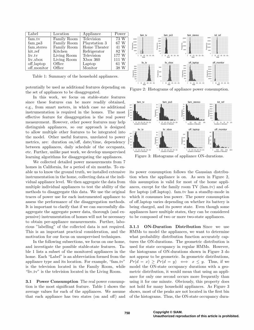
Figure 3: Histograms of appliance ON-durations.

its power consumption follows the Gaussian distribu-tion when the appliance is on. As seen in Figure 2,this assumption is valid for most of the home appli-ances, except for the family room TV (fam tv) and of-fice laptop (off laptop). fam tv has a standby-mode inwhich it consumes less power. The power consumptionof off laptop varies depending on whether its battery isbeing charged, and its power state. Even though someappliances have multiple states, they can be consideredto be composed of two or more two-state appliances.

3.1.1 ON-Duration Distribution Since we useHMMs to model the appliances, we want to determinewhat probability distribution function accurately cap-tures the ON-durations. The geometric distribution isused for state occupancy in regular HMMs. However,the histograms of ON-durations shown in Figure 3 donot appear to be geometric. In geometric distributions,Pr(d = x) ≥ Pr(d = y) ⇐⇒ x ≤ y. Thus, if wemodel the ON-state occupancy durations with a geo-metric distribution, it would mean that using an appli-ance for only one second occurs more frequently thanusing it for one minute. Obviously, this property doesnot hold for many household appliances. As Figure 3shows, most of the peaks are not located in the first binof the histograms. Thus, the ON-state occupancy dura-

750 Copyright © SIAM.Unauthorized reproduction of this article is prohibited.

fam_tv

Duration in Minutes

Fre

quen

cy

0

50

100

150

200

250

300

350

0 200 400 600 800 1000

fam_ps3

Duration in Minutes

Fre

quen

cy0

5

10

15

20

0 200 400 600 800 1000

fam_stereo

Duration in Minutes

Fre

quen

cy

0

20

40

60

80

100

120

0 200 400 600 800 1000

kit_ref

Duration in Minutes

Fre

quen

cy

0

500

1000

1500

2000

2500

0 20 40 60 80 100

liv_tv

Duration in Minutes

Fre

quen

cy

0

50

100

150

200

0 200 400 600 800 1000

liv_xbox

Duration in Minutes

Fre

quen

cy

0

10

20

30

40

50

0 200 400 600 800 1000

off_laptop

Duration in Minutes

Fre

quen

cy

0

50

100

150

200

250

300

0 200 400 600 800 1000

off_monitor

Duration in Minutes

Fre

quen

cy

0

5

10

15

0 200 400 600 800 1000

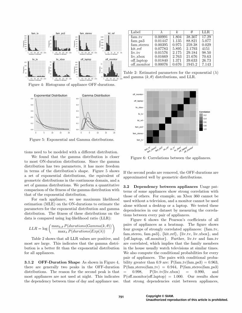
Figure 4: Histograms of appliance OFF-durations.

Exponential Distribution

0.0

0.1

0.2

0.3

0.4

0.5

0 5 10 15 20

Gamma Distribution

0.0

0.1

0.2

0.3

0.4

0.5

0 5 10 15 20

Figure 5: Exponential and Gamma distributions.

tions need to be modeled with a different distribution.We found that the gamma distribution is closer

to most ON-duration distributions. Since the gammadistribution has two parameters, it has more freedomin terms of the distribution’s shape. Figure 5 showsa set of exponential distributions, the equivalent ofgeometric distributions in the continuous domain, and aset of gamma distributions. We perform a quantitativecomparison of the fitness of the gamma distribution withthat of the exponential distribution.

For each appliance, we use maximum likelihoodestimation (MLE) on the ON-durations to estimate theparameters for the exponential distribution and gammadistribution. The fitness of these distributions on thedata is compared using log-likelihood ratio (LLR):

LLR = log

(maxk,θ P (durations|Gamma(k, θ))

maxλ P (durations|Exp(λ))

)Table 2 shows that all LLR values are positive, and

most are large. This indicates that the gamma distri-bution is a better fit than the exponential distributionfor all appliances.

3.1.2 OFF-Duration Shape As shown in Figure 4,there are generally two peaks in the OFF-durationdistributions. The reason for the second peak is thatmost appliances are not used at night. This indicatesthe dependency between time of day and appliance use.

Label λ k θ LLRfam tv 0.00991 1.804 38.307 17.29fam ps3 0.01447 1.135 88.821 5.077fam stereo 0.00395 0.975 259.38 0.029kit ref 0.07783 5.895 2.1793 4151liv tv 0.01576 2.175 29.184 98.50liv xbox 0.01669 2.763 21.676 70.63off laptop 0.01840 1.371 39.633 26.73off monitor 0.00076 0.676 1945.2 7.143

Table 2: Estimated parameters for the exponential (λ)and gamma (k, θ) distributions, and LLR.

fam_tv

fam_stereo

fam_ps3

kit_ref

liv_tv

liv_xbox

off_laptop

off_monitor

fam_tv

fam_stereo

fam_ps3kit_ref

liv_tv

liv_xbox

off_laptop

off_monitor

Correlation

0.2

0.4

0.6

0.8

1.0

Figure 6: Correlations between the appliances.

If the second peaks are removed, the OFF-durations areapproximated well by geometric distributions.

3.2 Dependency between appliances Usage pat-terns of some appliances show strong correlation withthose of others. For example, an Xbox 360 cannot beused without a television, and a monitor cannot be usedalone without a desktop or a laptop. We tested thesedependencies in our dataset by measuring the correla-tions between every pair of appliances.

Figure 6 shows the Pearson’s coefficients of allpairs of appliances as a heatmap. The figure showsfour groups of strongly correlated appliances: {fam tv,fam stereo, fam ps3}, {kit ref}, {liv tv, liv xbox}, and{off laptop, off monitor}. Further, liv tv and fam tvare correlated, which implies that the family membersin the house usually watch televisions at similar times.We also compute the conditional probabilities for everypair of appliances. The pairs with conditional proba-bility greater than 0.9 are: P(fam tv|fam ps3) = 0.963,P(fam stereo|fam tv) = 0.944, P(fam stereo|fam ps3)= 0.998, P(liv tv|liv xbox) = 0.990, andP(off monitor|off laptop) = 1.000. Our results showthat strong dependencies exist between appliances,

751 Copyright © SIAM.Unauthorized reproduction of this article is prohibited.

fam_tv

Time

Day

of t

he W

eek

MON

TUE

WED

THU

FRI

SAT

SUN

4 AM 8 AM 12 PM 4 PM 8 PM

Usage(%)

0

20

40

60

80

off_laptop

Time

Day

of t

he W

eek

MON

TUE

WED

THU

FRI

SAT

SUN

4 AM 8 AM 12 PM 4 PM 8 PM

Usage(%)

0

20

40

60

80

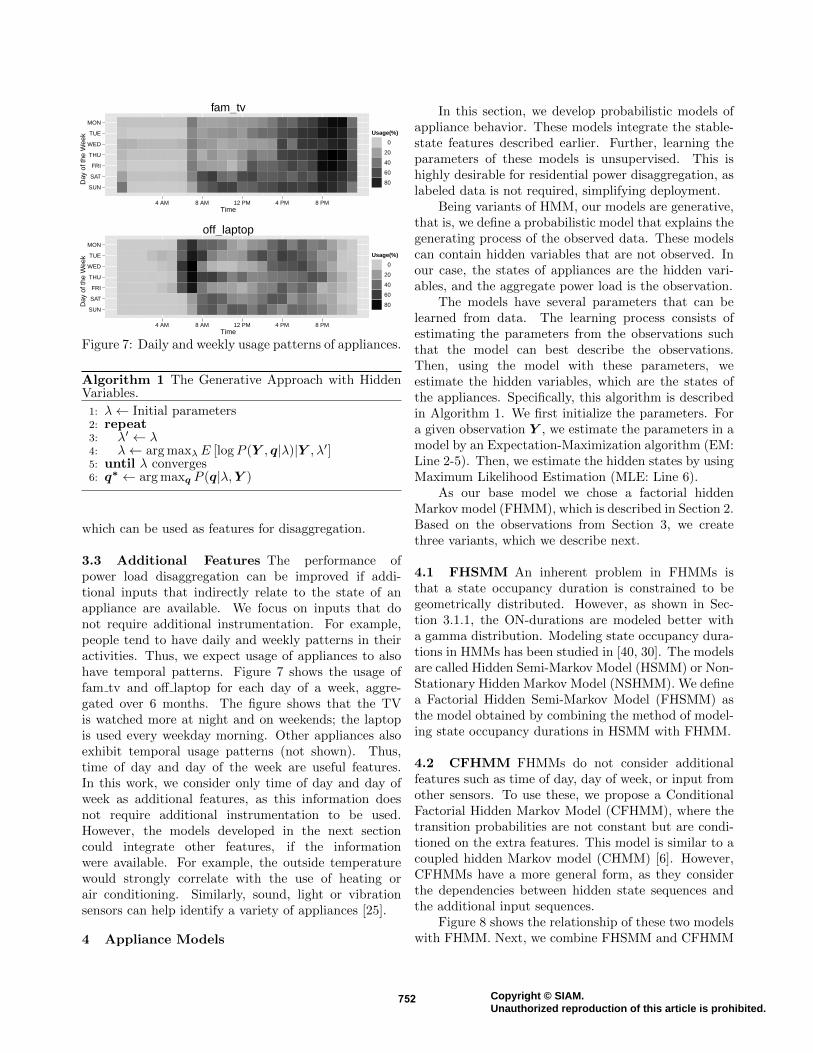
Figure 7: Daily and weekly usage patterns of appliances.

Algorithm 1 The Generative Approach with HiddenVariables.

1: λ← Initial parameters2: repeat3: λ′ ← λ4: λ← arg maxλE [logP (Y , q|λ)|Y , λ′]5: until λ converges6: q∗ ← arg maxq P (q|λ,Y )

which can be used as features for disaggregation.

3.3 Additional Features The performance ofpower load disaggregation can be improved if addi-tional inputs that indirectly relate to the state of anappliance are available. We focus on inputs that donot require additional instrumentation. For example,people tend to have daily and weekly patterns in theiractivities. Thus, we expect usage of appliances to alsohave temporal patterns. Figure 7 shows the usage offam tv and off laptop for each day of a week, aggre-gated over 6 months. The figure shows that the TVis watched more at night and on weekends; the laptopis used every weekday morning. Other appliances alsoexhibit temporal usage patterns (not shown). Thus,time of day and day of the week are useful features.In this work, we consider only time of day and day ofweek as additional features, as this information doesnot require additional instrumentation to be used.However, the models developed in the next sectioncould integrate other features, if the informationwere available. For example, the outside temperaturewould strongly correlate with the use of heating orair conditioning. Similarly, sound, light or vibrationsensors can help identify a variety of appliances [25].

4 Appliance Models

In this section, we develop probabilistic models ofappliance behavior. These models integrate the stable-state features described earlier. Further, learning theparameters of these models is unsupervised. This ishighly desirable for residential power disaggregation, aslabeled data is not required, simplifying deployment.

Being variants of HMM, our models are generative,that is, we define a probabilistic model that explains thegenerating process of the observed data. These modelscan contain hidden variables that are not observed. Inour case, the states of appliances are the hidden vari-ables, and the aggregate power load is the observation.

The models have several parameters that can belearned from data. The learning process consists ofestimating the parameters from the observations suchthat the model can best describe the observations.Then, using the model with these parameters, weestimate the hidden variables, which are the states ofthe appliances. Specifically, this algorithm is describedin Algorithm 1. We first initialize the parameters. Fora given observation Y , we estimate the parameters in amodel by an Expectation-Maximization algorithm (EM:Line 2-5). Then, we estimate the hidden states by usingMaximum Likelihood Estimation (MLE: Line 6).

As our base model we chose a factorial hiddenMarkov model (FHMM), which is described in Section 2.Based on the observations from Section 3, we createthree variants, which we describe next.

4.1 FHSMM An inherent problem in FHMMs isthat a state occupancy duration is constrained to begeometrically distributed. However, as shown in Sec-tion 3.1.1, the ON-durations are modeled better witha gamma distribution. Modeling state occupancy dura-tions in HMMs has been studied in [40, 30]. The modelsare called Hidden Semi-Markov Model (HSMM) or Non-Stationary Hidden Markov Model (NSHMM). We definea Factorial Hidden Semi-Markov Model (FHSMM) asthe model obtained by combining the method of model-ing state occupancy durations in HSMM with FHMM.

4.2 CFHMM FHMMs do not consider additionalfeatures such as time of day, day of week, or input fromother sensors. To use these, we propose a ConditionalFactorial Hidden Markov Model (CFHMM), where thetransition probabilities are not constant but are condi-tioned on the extra features. This model is similar to acoupled hidden Markov model (CHMM) [6]. However,CFHMMs have a more general form, as they considerthe dependencies between hidden state sequences andthe additional input sequences.

Figure 8 shows the relationship of these two modelswith FHMM. Next, we combine FHSMM and CFHMM

752 Copyright © SIAM.Unauthorized reproduction of this article is prohibited.

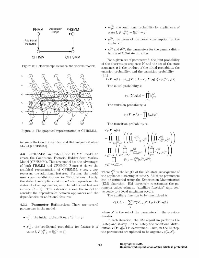
FHMM FHSMM

CFHMM CFHSMM

Distribution Shape

Additional Features

Figure 8: Relationships between the various models.

P(d3=3)

P(d1=2)

P(d2=3)

P(d1=5)

ON ON OFF ON

ON ON ON OFF

ON ON OFF OFF

yt-1 yt yt+1 yt+2

OFF

OFF

ON

yt-2y

q3

q2

q1

1 2 2 11c2

3 0 0 23c1

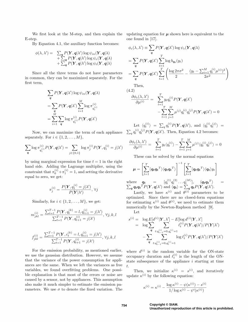
Figure 9: The graphical representation of CFHSMM.

to create the Conditional Factorial Hidden Semi-MarkovModel (CFHSMM).

4.3 CFHSMM We extend the FHMM model tocreate the Conditional Factorial Hidden Semi-MarkovModel (CFHSMM). This new model has the advantagesof both FHSMM and CFHMM. Figure 9 shows thegraphical representation of CFHSMM. c1, c2, . . . , cKrepresent the additional features. Further, the modeluses a gamma distribution for ON-durations. Lastly,the state of an appliance at time t also depends on thestates of other appliances, and the additional featuresat time (t − 1). This extension allows the model toconsider the dependencies between appliances and thedependencies on additional features.

4.3.1 Parameter Estimations There are severalparameters in the model.

• π(i)j , the initial probabilities, P (q

(i)1 = j)

• f(i)jkl, the conditional probability for feature k of

value l, P (c(k)t−1 = l|q(i)t = j)

• m(i)jkl, the conditional probability for appliance k of

state l, P (q(k)t−1 = l|q(i)t = j)

• µ(i), the mean of the power consumption for theappliance i

• κ(i) and θ(i), the parameters for the gamma distri-bution of ON-state duration

For a given set of parameter λ, the joint probabilityof the observation sequence Y and the set of the statesequences q is the product of the initial probability, theemission probability, and the transition probability.(4.1)

P (Y , q|λ) = ψin(Y , q|λ) · ψe(Y , q|λ) · ψt(Y , q|λ)

The initial probability is

ψin(Y , q|λ) =

M∏i=1

π(i)

q(i)1

The emission probability is

ψe(Y , q|λ) =

T∏t=1

bqt(yt)

The transition probability is

ψt(Y , q|λ)

=

M∏i=1

∏t:q

(i)t =0

M∏j=1

m(i)

q(i)t+1jq

(j)t

K∏j=1

f(i)

q(i)t+1jc

(j)t

∏

t:q(i)t =1

M∏j=1:i 6=j

m(i)

q(i)t+1jq

(j)t

K∏j=1

f(i)

q(i)t+1jc

(j)t

∏

t:q(i)t =1,q

(i)t−1=0

P (d = `(i)t |κ(i), θ(i))

where `(i)t is the length of the ON-state subsequence of

the appliance i starting at time t. All these parameterscan be estimated using the Expectation Maximization(EM) algorithm. EM iteratively re-estimates the pa-rameter values using an “auxiliary function” until con-vergence to a local maximum occurs.

The auxiliary function to be maximized is

φ(λ, λ′) =∑q

P (Y , q|λ′) logP (Y , q|λ)

where λ′ is the set of the parameters in the previousiteration.

In each iteration, the EM algorithm performs theE-step and M-step. In the E-step, the conditional distri-bution P (Y , q|λ′) is determined. Then, in the M-step,the parameters are updated to be arg maxλ φ(λ, λ′).

753 Copyright © SIAM.Unauthorized reproduction of this article is prohibited.

We first look at the M-step, and then explain theE-step.

By Equation 4.1, the auxiliary function becomes:

φ(λ, λ′) =∑

q P (Y , q|λ′) logψin(Y , q|λ)

+∑

q P (Y , q|λ′) logψe(Y , q|λ)

+∑

q P (Y , q|λ′) logψt(Y , q|λ)

Since all the three terms do not have parametersin common, they can be maximized separately. For thefirst term, ∑

q

P (Y , q|λ′) logψin(Y , q|λ)

=∑q

P (Y , q|λ′)M∑i=1

log π(i)

q(i)1

=

M∑i=1

∑q

log π(i)

q(i)1

P (Y , q|λ′)

Now, we can maximize the term of each applianceseparately. For i ∈ {1, 2, . . . ,M},∑q

log π(i)

q(i)1

P (Y , q|λ′) =∑

j∈{0,1}

log π(i)j P (Y , q

(i)1 = j|λ′)

by using marginal expression for time t = 1 in the righthand side. Adding the Lagrange multiplier, using the

constraint that π(i)0 +π

(i)1 = 1, and setting the derivative

equal to zero, we get:

π(i)j =

P (Y , q(i)1 = j|λ′)

P (Y |λ′), ∀j

Similarly, for i ∈ {1, 2, . . . ,M}, we get:

m(i)jkl =

∑T−1t=1 P (Y , q

(k)t = l, q

(i)t+1 = j|λ′)∑T−1

t=1 P (Y , q(i)t+1 = j|λ′)

, ∀j, k, l

f(i)jkl =

∑T−1t=1 P (Y , c

(k)t = l, q

(i)t+1 = j|λ′)∑T−1

t=1 P (Y , q(i)t+1 = j|λ′)

, ∀j, k, l

For the emission probability, as mentioned earlier,we use the gaussian distribution. However, we assumethat the variance of the power consumption for appli-ances are the same. When we left the variances as freevariables, we found overfitting problems. One possi-ble explanation is that most of the errors or noise arecaused by a sensor, not by appliances. This assumptionalso make it much simpler to estimate the emission pa-rameters. We use σ to denote the fixed variation. The

updating equation for µ shown here is equivalent to theone found in [17].

φe(λ, λ′) ≡

∑q

P (Y , q|λ′) logψe(Y , q|λ)

=∑q

P (Y , q|λ′)T∑t=1

log bqt(yt)

=∑q

P (Y , q|λ′)T∑t=1

(log 2πσ2

2−

(yt −∑Mi=1 q

(i)t µ(i))2

2σ2

)Then,

(4.2)

∂φe(λ, λ′)

∂µ(i)=

T∑t=1

ytq(i)t P (Y , q|λ′)

−T∑t=1

M∑j=1

µ(j)q(i)t q

(j)t P (Y , q|λ′) = 0

Let 〈q(i)t 〉 =∑q q

(i)t P (Y , q|λ′), and 〈q(i)t q

(j)t 〉 =∑

q q(i)t q

(j)t P (Y , q|λ′). Then, Equation 4.2 becomes:

∂φe(λ, λ′)

∂µ(i)=

T∑t=1

yt〈q(i)t 〉 −T∑t=1

M∑j=1

µ(j)〈q(i)t q(j)t 〉 = 0

These can be solved by the normal equations

µ =

[T∑t=1

〈qtqtT 〉〈qtqtT 〉

]−1 [ T∑t=1

〈qtqtT 〉〈qt〉yt

]

where qt = [q(1)t q

(2)t . . . q

(M)t ], 〈qtqtT 〉 =∑

q qtqtTP (Y , q|λ′) and 〈qt〉 =

∑q qtP (Y , q|λ′).

Lastly, we have κ(i) and θ(i) parameters to beoptimized. Since there are no closed-form equationsfor estimating κ(i) and θ(i), we need to estimate themnumerically by the Newton-Raphson method [9].

Let

s(i) = logE[d(i)|Y , λ′]− E[log d(i)|Y , λ′]= log

∑q

∑t:q

(i)t−1=0,q

(i)t =1

`(i)t P (Y , q|λ′)/P (Y |λ′)

−∑q

∑t:q

(i)t−1=0,q

(i)t =1

log `(i)t P (Y , q|λ′)/P (Y |λ′)

where d(i) is the random variable for the ON-stateoccupancy duration and `

(i)t is the length of the ON-

state subsequence of the appliance i starting at timet.

Then, we initialize κ(i) = s(i), and iterativelyupdate κ(i) by the following equation:

κ(i) = κ(i) − log κ(i) − ψ(κ(i))− s(i)

1/ log κ(i) − ψ′(κ(i))

754 Copyright © SIAM.Unauthorized reproduction of this article is prohibited.

where ψ is the digamma function and ψ′ is the trigammafunction.

After iteratively estimating κ(i), we set

θ(i) = E[d(i)|Y , λ′](κ(i))−1

=

∑q

∑t:q

(i)t−1=0,q

(i)t =1

`(i)t

P (Y , q|λ′)P (Y |λ′)

(κ(i))−1

These updating equations complete the M-step inour EM algorithm. In contrast to the M-step, the exactinference of the conditional distribution P (Y , q|λ′) inthe E-step is computationally intractable as mentionedin [17]. There are alternative ways to approximate theinference, including Gibbs sampling and the mean fieldapproximation [17]. Here, we use Gibbs sampling [16],one of the Monte Carlo methods, because of its simplic-ity. Since Gibbs sampling is a well-known tool and easyto adapt to any model, we omit its details.

4.3.2 Hidden State Estimation The goal of theenergy load disaggregation is to discover the states ofappliances. We are more interested in the sequencesof the hidden variables in the CFHSMM than theparameters in the model. After learning the parameters,we need to use Maximum Likelihood Estimation (MLE)to estimate the sequences of the hidden variables.

In other words, we want to find q∗ such that

q∗ = arg maxq

P (Y , q|λ)

The Viterbi algorithm can efficiently estimate thehidden states for HMMs. It uses dynamic program-ming to solve the optimization problem. However, dy-namic programming for CFHSMMs is computationallyintractable [17]. Thus, we use simulated annealing(SA) [26] to find q∗. For the same reason as with Gibbssampling, we omit the explanation of SA.

5 Experimental Results

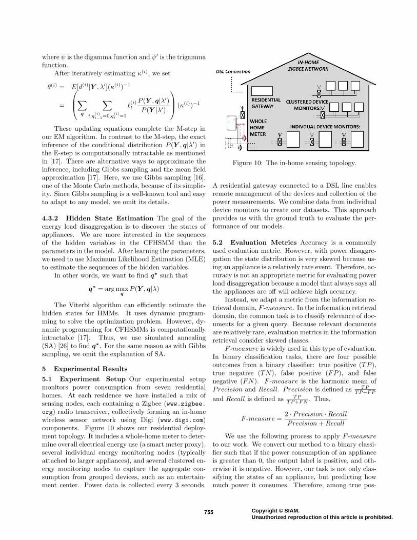
5.1 Experiment Setup Our experimental setupmonitors power consumption from seven residentialhomes. At each residence we have installed a mix ofsensing nodes, each containing a Zigbee (www.zigbee.org) radio transceiver, collectively forming an in-homewireless sensor network using Digi (www.digi.com)components. Figure 10 shows our residential deploy-ment topology. It includes a whole-home meter to deter-mine overall electrical energy use (a smart meter proxy),several individual energy monitoring nodes (typicallyattached to larger appliances), and several clustered en-ergy monitoring nodes to capture the aggregate con-sumption from grouped devices, such as an entertain-ment center. Power data is collected every 3 seconds.

Figure 10: The in-home sensing topology.

A residential gateway connected to a DSL line enablesremote management of the devices and collection of thepower measurements. We combine data from individualdevice monitors to create our datasets. This approachprovides us with the ground truth to evaluate the per-formance of our models.

5.2 Evaluation Metrics Accuracy is a commonlyused evaluation metric. However, with power disaggre-gation the state distribution is very skewed because us-ing an appliance is a relatively rare event. Therefore, ac-curacy is not an appropriate metric for evaluating powerload disaggregation because a model that always says allthe appliances are off will achieve high accuracy.

Instead, we adapt a metric from the information re-trieval domain, F -measure. In the information retrievaldomain, the common task is to classify relevance of doc-uments for a given query. Because relevant documentsare relatively rare, evaluation metrics in the informationretrieval consider skewed classes.

F -measure is widely used in this type of evaluation.In binary classification tasks, there are four possibleoutcomes from a binary classifier: true positive (TP ),true negative (TN), false positive (FP ), and falsenegative (FN). F -measure is the harmonic mean ofPrecision and Recall. Precision is defined as TP

TP+FP

and Recall is defined as TPTP+FN . Thus,

F -measure =2 · Precision ·RecallPrecision+Recall

We use the following process to apply F -measureto our work. We convert our method to a binary classi-fier such that if the power consumption of an applianceis greater than 0, the output label is positive, and oth-erwise it is negative. However, our task is not only clas-sifying the states of an appliance, but predicting howmuch power it consumes. Therefore, among true pos-

755 Copyright © SIAM.Unauthorized reproduction of this article is prohibited.

Shape

F−

Mea

sure

0.5

0.6

0.7

0.8

0.9

1.0

2 4 6 8 10

Model

FHMM

FHSMM

Figure 11: The effect of ON-duration shape.

itives, we consider predictions that differ significantlyfrom ground truth as incorrect. More specifically, wesplit the true positives into two categories, accurate truepositive (ATP), and inaccurate true positive (ITP). Wedistinguish the predictions as follows. Let x be the pre-dicted value, and x0 be the ground truth value.

• When x = 0 and x0 = 0, the prediction is truenegative (TN).

• When x = 0 and x0 > 0, the prediction is falsenegative (FN).

• When x > 0 and x0 = 0, the prediction is falsepositive (FP).

• When x > 0, x0 > 0, and |x−x0|x0

≤ ρ, the predictionis an accurate true positive (ATP).

• When x > 0, x0 > 0, and |x−x0|x0

> ρ, the predictionis an inaccurate true positive (ITP).

where ρ is a threshold.We redefine Precision and Recall such

that Precision = ATPATP+ITP+FP and Recall =

ATPATP+ITP+FN . F -measure remains the harmonicmean of the new Precision and Recall. We use thenew F -measure as our metric with ρ = 0.2 in theevaluation. Most appliances in our evaluation havestandard variations of around 20% of their means. Forexample, the power consumption of kit ref has standarddeviation of 15W, where its mean is 82W.

Since the output of the unsupervised models do nothave labels on each appliance, we compute F -measurefor all possible mappings, and take the maximum valuesas their performance.

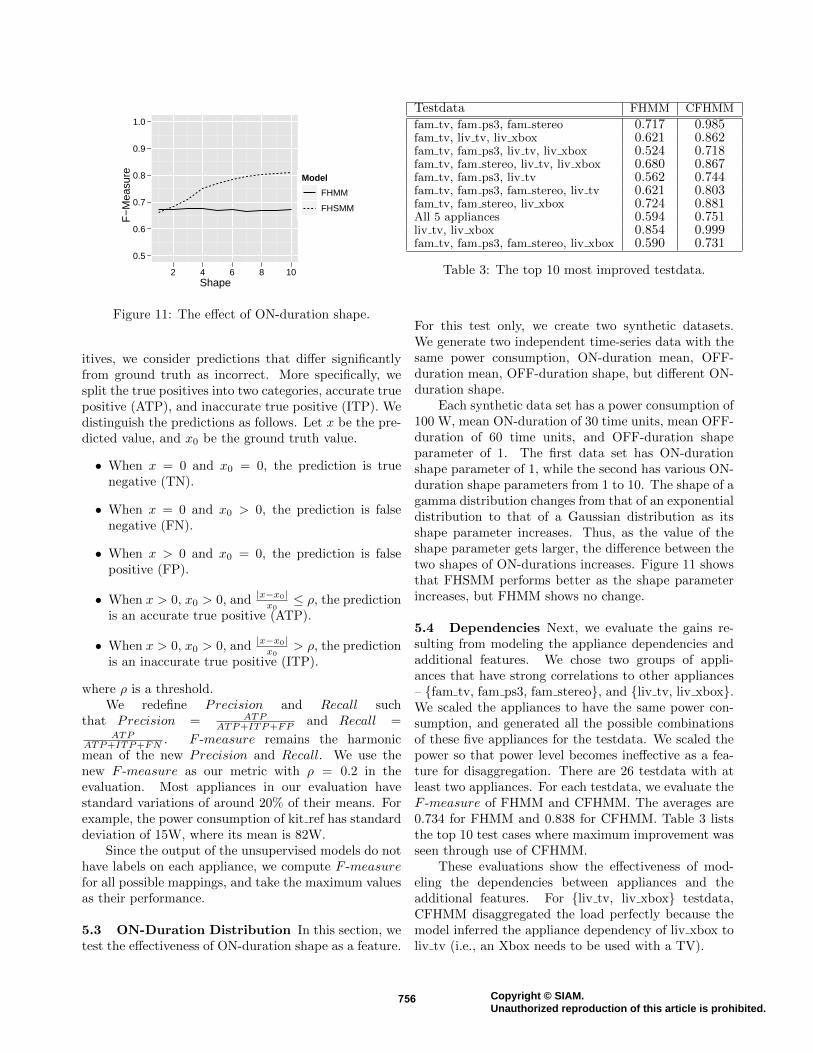
5.3 ON-Duration Distribution In this section, wetest the effectiveness of ON-duration shape as a feature.

Testdata FHMM CFHMM

fam tv, fam ps3, fam stereo 0.717 0.985fam tv, liv tv, liv xbox 0.621 0.862fam tv, fam ps3, liv tv, liv xbox 0.524 0.718fam tv, fam stereo, liv tv, liv xbox 0.680 0.867fam tv, fam ps3, liv tv 0.562 0.744fam tv, fam ps3, fam stereo, liv tv 0.621 0.803fam tv, fam stereo, liv xbox 0.724 0.881All 5 appliances 0.594 0.751liv tv, liv xbox 0.854 0.999fam tv, fam ps3, fam stereo, liv xbox 0.590 0.731

Table 3: The top 10 most improved testdata.

For this test only, we create two synthetic datasets.We generate two independent time-series data with thesame power consumption, ON-duration mean, OFF-duration mean, OFF-duration shape, but different ON-duration shape.

Each synthetic data set has a power consumption of100 W, mean ON-duration of 30 time units, mean OFF-duration of 60 time units, and OFF-duration shapeparameter of 1. The first data set has ON-durationshape parameter of 1, while the second has various ON-duration shape parameters from 1 to 10. The shape of agamma distribution changes from that of an exponentialdistribution to that of a Gaussian distribution as itsshape parameter increases. Thus, as the value of theshape parameter gets larger, the difference between thetwo shapes of ON-durations increases. Figure 11 showsthat FHSMM performs better as the shape parameterincreases, but FHMM shows no change.

5.4 Dependencies Next, we evaluate the gains re-sulting from modeling the appliance dependencies andadditional features. We chose two groups of appli-ances that have strong correlations to other appliances– {fam tv, fam ps3, fam stereo}, and {liv tv, liv xbox}.We scaled the appliances to have the same power con-sumption, and generated all the possible combinationsof these five appliances for the testdata. We scaled thepower so that power level becomes ineffective as a fea-ture for disaggregation. There are 26 testdata with atleast two appliances. For each testdata, we evaluate theF -measure of FHMM and CFHMM. The averages are0.734 for FHMM and 0.838 for CFHMM. Table 3 liststhe top 10 test cases where maximum improvement wasseen through use of CFHMM.

These evaluations show the effectiveness of mod-eling the dependencies between appliances and theadditional features. For {liv tv, liv xbox} testdata,CFHMM disaggregated the load perfectly because themodel inferred the appliance dependency of liv xbox toliv tv (i.e., an Xbox needs to be used with a TV).

756 Copyright © SIAM.Unauthorized reproduction of this article is prohibited.

Home ID Num. of Appliances FHMM CFHSMMHome 1 4 0.983 0.998Home 2 6 0.899 0.930Home 3 6 0.859 0.881Home 4 7 0.625 0.693Home 5 8 0.713 0.781Home 6 8 0.641 0.722Home 7 10 0.796 0.874

Table 4: The evaluations on several homes.

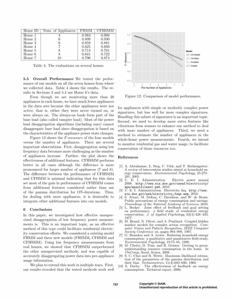
5.5 Overall Performance We tested the perfor-mance of our models on all the seven homes from wherewe collected data. Table 4 shows the results. The re-sults in Sections 3 and 5.4 use Home 6’s data.

Even though we are monitoring more than 20appliances in each house, we have much fewer appliancesin the data sets because the other appliances were notactive, that is, either they were never turned on, orwere always on. The always-on loads form part of thebase load (also called vampire load). Most of the powerload disaggregation algorithms (including ours) cannotdisaggregate base load since disaggregation is based onthe characteristics of the appliance power state changes.

Figure 12 shows the F -measure of the four modelsversus the number of appliances. There are severalimportant observations. First, disaggregation using lowfrequency data becomes more challenging as the numberof appliances increase. Further, the plot shows theeffectiveness of additional features. CFHSMM performsbetter in all cases although the difference is morepronounced for larger number of appliances (7 and 8).The difference between the performance of CFHSMMand CFHMM is minimal indicating that for this dataset most of the gain in performance of CFHSMM comesfrom additional features considered rather than useof the gamma distribution for ON-durations. Thus,for dealing with more appliances, it is desireable tointegrate other additional features into our models.

6 Conclusions

In this paper, we investigated how effective unsuper-vised disaggregation of low frequency power measure-ments is. This is an important topic, as an effectivemethod of this type could facilitate residential electric-ity conservation efforts. We considered a existing modelFHMM and three new models (FHSMM, CFHMM andCFHSMM). Using low frequency measurements fromreal homes, we showed that CFHSMM outperformedthe other unsupervised methods, and was capable ofaccurately disaggregating power data into per-applianceusage information.

We plan to extend this work in multiple ways. First,our results revealed that the tested methods work well

The Number of Appliances

F−

Mea

sure

0.5

0.6

0.7

0.8

0.9

1.0

2 3 4 5 6 7 8

Model

CFHSMM

CFHMM

FHSMM

FHMM

Figure 12: Comparison of model performance.

for appliances with simple or modestly complex powersignatures, but less well for more complex signatures.Handling this subset of signatures is an important topic.Second, we need to develop more extra features likevibrations from sensors to enhance our method to dealwith more number of appliances. Third, we need amethod to estimate the number of appliances in thewhole-home power measurements. Fourth, we intendto monitor residential gas and water usage, to facilitateconservation of those resources too.

References

[1] A. Abrahamse, L. Steg, C. Vlek, and T. Rothengatter.A review of intervention studies aimed at household en-ergy conservation. Environmental Psychology, 25:273–291, 2005.

[2] U. E. I. Administration. Electric power annual2008. http://www.eia.doe.gov/cneaf/electricity/epa/epaxlfilees1.pdf, 2010.

[3] U. E. I. Administration. Electricity faq. http://www.eia.doe.gov/ask/electricity_faqs.asp, 2010.

[4] S. Attari, M. DeKay, C. Davidson, and W. de Bruin.Public perceptions of energy consumption and savings.Proceedings of the National Academy of Sciences, 2010.

[5] L. Becker. Joint effect of feedback and goal settingon performance: a field study of residential energyconservation. J. of Applied Psychology, 63(4):428–433,1977.

[6] M. Brand, N. Oliver, and A. Pentland. Coupled hiddenmarkov models for complex action recognition. Com-puter Vision and Pattern Recognition, IEEE ComputerSociety Conference on, pages 994–999, 1997.

[7] G. Brandon and A. Lewis. Reducing household energyconsumption: a qualitative and quantitative field study.Environmental Psychology, 19:75–85, 1999.

[8] M. Chetty, D. Tran, and R. Grinter. Getting to green:understanding resource consumption in the home. InUbiComp, Seoul, Korea, 2008.

[9] S. C. Choi and R. Wette. Maximum likelihood estima-tion of the parameters of the gamma distribution andtheir bias. Technometrics, 11(4):683–690, 1969.

[10] S. Darby. The effectiveness of feedback on energyconsumption. Technical report, 2006.

757 Copyright © SIAM.Unauthorized reproduction of this article is prohibited.

[11] L. Farinaccio and R. Zmeureanu. Using a pattern recog-nition approach to disaggregate the total electricity con-sumption in a house into the major end uses. Energyand Buildings, 30:245–259, 1999.

[12] C. Fischer. Feedback on household electricity consump-tion: a tool for saving energy? Energy Efficiency, 1:79–104, 2008.

[13] R. Fitch. New meter helps buyer save energy. Houseand Home, 51(5):58, 1977.

[14] G. Gardner and P. Stern. The short list: the most ef-fective actions U.S. households can take to curb climatechange. Environment Magazine, 2008.

[15] S. Geman and D. Geman. Stochastic relaxation, gibbsdistributions, and the bayesian restoration of images.IEEE Transactions on Pattern Analysis and MachineIntelligence, 6:721–741, 1984.

[16] Z. Ghahramani and M. I. Jordan. Factorial hiddenmarkov models. Machine Learning, 29:245–273, 1997.

[17] G. Hart. Nonintrusive appliance load monitoring.Proceedings of the IEEE, 80(2):1870–1891, 1992.

[18] S. Hayes and J. Cone. Reduction of residential con-sumption of electricity through simple monthly feed-back. Applied Behavior Analysis, 14(1):81–88, 1981.

[19] J. V. Houwelingen and F. V. Raaij. The effect of goal-setting and daily electronic feedback on in-home energyuse. Consumer Research, 16:98–105, 1989.

[20] E. Howell. How switches produce electrical noise. IEEEtransactions on electromagnetic compatibility, EMC-21(3):162–170, 1979.

[21] M. Ito, R. Uda, S. Ichimura, K. Tago, T. Hoshi, andY. Matsushita. A method of appliance detection basedon features of power waveform. In IEEE Symposium onApplications and the Internet, Tokyo, Japan, 2004.

[22] T. Kao, H. Cho, D. Lee, T. Toyomura, and T. Ya-mazaki. Appliance recognition from electric current sig-nals for information-energy integrated network in homeenvironments. In International Conference on SmartHomes and Health Telematics, Tours, France, 2009.

[23] W. Kempton and L. Layne. The consumer’s energyanalysis environment. Energy Policy, 22(10):857–866,1994.

[24] Y. Kim, T. Schmid, Z. Charbiwala, and M. Srivas-tava. Viridiscope: design and implementation of a finegrained power monitoring system for homes. In Ubi-Comp, Orlando, FL, 2009.

[25] S. Kirkpatrick, C. D. Gelatt, and M. P. Vec-chi. Optimization by simulated annealing. Science,220(4598):pp. 671–680, 1983.

[26] R. Kohlenberg, T. Phillips, and W. Proctor. A be-havioral analysis of peaking in residential electrical-energy consumers. Applied Behavior Analysis, 9(1):13–18, 1976.

[27] A. Krogh, M. Brown, S. Mian, K. Sjolander, andD. Haussler. Hidden Markov models in computationalbiology. Molecular Biology, 235:1501–1531, 1994.

[28] C. Laughman, K. Lee, R. Cox, S. Shaw, S. Leeb,L. Norford, and P. Armstrong. Power signature anal-ysis. IEEE Power and Energy, 1(2):56–63, 2003.

[29] S. Levinson. Continuously variable duration hiddenmarkov models for automatic speech recognition. Com-puter Speech and Language, 1(1):29 – 45, 1986.

[30] G. Lin, S. Lee, J. Hsu, and W. Jih. Applyingpower meters for appliance recognition on the electricpanel. In IEEE Industrial Electronics and Applications,Taichung, Taiwan, 2010.

[31] H. Matthews, L. Soibelman, M. Berges, and E. Gold-man. Automatically disaggregating the total electricalload in residential buildings: a profile of the requiredsolution. In Intelligent Computing in Engineering, Ply-mouth, UK, 2008.

[32] L. Norford and S. Leeb. Non-intrusive electrical loadmonitoring in commercial buildings based on steady-state and transient load-detection algoritms. Energyand Buildings, 24:51–64, 1996.

[33] S. Patel, S. Gupta, and M. Reynolds. The design andevaluation of an end-user-deployable, whole house, con-tactless power consumption sensor. In Human factorsin computing systems, Atlanta, GA, 2010.

[34] S. Patel, T. Robertson, J. Kientz, M. Reynolds, andG. Abowd. At the flick of a switch: detecting andclassifying unique electrical events on the residentialpower line. In UbiComp, Innsbruck, Austria, 2007.

[35] A. Prudenzi. A neuron nets based procedure for iden-tifying domestic appliances pattern-of-use from energyrecordings at meter panel. IEEE Power EngineeringSociety Winter Meeting, 2:491–496, 2002.

[36] L. Rabiner. A tutorial on hidden Markov models andselected applications in speech recognition. Proceedingsof the IEEE, 77(2):257–286, 1989.

[37] Y. Riche, J. Dodge, and R. Metoyer. Studying always-on electricity feedback in the home. In Human factorsin computing systems, Atlanta, GA, 2010.

[38] B. Ritchie, G. McDougall, and J. Claxton. Complexi-ties of household energy consumption and conservation.Consumer Research, 8(3):233–242, 1981.

[39] M. Russell and R. Moore. Explicit modelling of stateoccupancy in hidden markov models for automaticspeech recognition. volume 10, pages 5 – 8, 1985.

[40] T. Saitoh, Y. Aota, T. Osaki, R. Konishi, and K. Sug-ahara. Current sensor based non-intrusive appliancerecognition for intelligent outlet. In Int. Technical Con-ference on Circuits/Systems, Computers and Commu-nications, Shimonoseki City, Japan, 2008.

[41] C. Seligman and J. Darley. Feedback as a meansof decreasing residential energy consumption. AppliedPsychology, 62(4):363–368, 1977.

[42] H. Serra, J. Correia, A. Gano, A. de Campos, andI. Teixeira. Domestic power consumption measurementand automatic home appliance detection. In IEEE In-telligent Signal Processing workshop, Algarve, Portugal,2005.

[43] R. Sexton, N.Johnson, and A. Konakayama. Consumerresponse to continuous-display electricity-use monitorsin a time-of-use pricing experiment. Consumer Re-search, 14(1):55–62, 1987.

[44] P. Stern. What psychology knows about energy con-servation. American Physchologist, 47(10):1224–1232,1992.

[45] K. Suzuki, S. Inagaki, T. Suzuki, H. Nakamura, andK. Ito. Nonintrusive appliance load monitoring basedon integer programming. In Int. Conference on Instru-mentation, Control and Information Technology, Tokyo,Japan, 2008.

[46] T. Ueno, F. Sano, O. Saeki, and K. Tsuji. Effectivenessof an energy-consumption information system on energysavings in residential houses based on monitored data.Applied Energy, 83:166–183, 2006.

[47] R. Vines. Noise on residential power distribution cir-cuits. IEEE transactions on electromagnetic compati-bility, EMC-26(4):161–168, 1984.

[48] R. Watson, M. Zinyousera, and R. M. (editors). Tech-nologies, policies and measures for mitigating climatechange. Technical report, 1996.

[49] N. Yadwadkar, C. Bhattacharyya, and K. Gopinath.Discovery of application workloads from network filetraces. In USENIX FAST, San Jose, CA, 2010.

758 Copyright © SIAM.Unauthorized reproduction of this article is prohibited.