Diffusion Measurements of Ethane in Activated

Carbon

by

PARINAZ MAKHTOUMI

A thesis submitted in partial fulfillment of the requirements for the degree of

Master of Science.

in

CHEMICAL ENGINEERING

Department of Chemical and Materials Engineering

University of Alberta

c© PARINAZ MAKHTOUMI, 2016

Abstract

Increasing demand for energy in the world has made industries to look for economically

efficient methods to produce energy. One possible approach is to increase natural gas

productions, due to its cleanliness and lower price. However, energy consumption of the

cryogenic processes is high in natural gas processing plants. Adsorptive separations are

becoming widespread in various industries such as oil and gas as a promising alternative to

the conventional cryogenic processes. Activated carbons are among the most attractive

porous materials used in adsorption processes, due to their high internal surface areas

and ease of availability in the market. They exhibit bimodal pore size distributions,

comprising microporous structure throughout a network of larger macropores. This makes

them interesting and challenging adsorbents in adsorption studies.

The separation of ethane from natural gas is one of the important processes in gas

processing plants. Ethane is highly needed as feedstock for ethylene production plants.

In this thesis, adsorption kinetics of ethane on activated carbon was studied using Zero

Length Column (ZLC) technique. ZLC is a useful chromatographic method to study

equilibrium and kinetics of adsorption. It is known as a fast and easy lab-scale technique

for adsorbent screenings and diffusion studies. In ZLC, external heat and mass transfer

resistances and dispersion are eliminated by the use of low adsorbate concentration, small

amount of adsorbent and high flow rates. In the experiments, the adsorbent sample is

first pre-equilibrated with the test gas for a sufficient time. The kinetics and equilibrium

information can be obtained from the desorption curve when the flow is switched to pure

purge gas under controlled conditions.

ii

The experimental set-up was developed during this project. System characterization

experiments such as dead volume measurements, detector selection, detector’s response

time calculations were performed and are discussed in detail. ZLC measurements were

carried out to study the controlling diffusion mechanism and obtain the diffusivity values.

By performing low concentration experiments, diffusion in macropores found to be the

controlling resistance. Among the various mechanisms, molecular and Knudsen diffusion

were identified to be important.

iii

To all courageous girls around the world who go beyond the traditional

norms and become the leaders of their own lives.

Acknowledgements

I would first like to thank my thesis supervisor, Dr. Arvind Rajendran for his countless

advice, motivation and active collaboration during this project. I am deeply grateful for

giving me the opportunity to work in his research group. I broadened my knowledge and

professional skills during our weekly individual and group meetings. Being a member of

a multi-cultural group was a great experience. I really enjoyed our weekly group lunches

and Friday evenings in the Faculty Club where we talked about movies, cultures and

politics.

I acknowledge Ali and his wife who helped me to start my journey of life in Canada;

I wish them a happy life together with their son Sadra. I am sincerely grateful to my

colleagues, Ali and Ashwin for their help in developing the ZLC experimental set-up, and

their insights through the project, Libardo who assisted me on my thesis by providing

supplementary materials, Gokul, Nagesh and Nick for inviting me to their activities on

the weekends. Thank you guys, it was really fun hanging out with you. I would like

to also thank Adolfo, Dave, Johan, and Behnam for their support during my project.

Gratitude for helping me with my work is also due to James Sawada with his guidance

and advice on the experimental aspects.

I am sincerely grateful to Weizhu An for her advices on the experiments. I am also

grateful to Dr. De Klerk and his student Giselle Uzcategui who helped me to conduct

mercury porosimetry experiments; I wish her the best of luck in her PhD program. I

would like to thank Masoud Jahandar Lashaki for his help in experimental measurement

of nitrogen adsorption. I would also thank Artin Afacan, Kevin Heidebrecht and Les

Dean who collaborated and helped me in this project at University of Alberta.

My thanks to Navid for patiently listening to my worries during various stages of

this project, and giving me his thoughts and comments on the text of this thesis. I

acknowledge Dr. Motamedi for his great contribution in reviewing my thesis and our

v

Sugar Bowl sessions after work in the freezing Edmonton winters. Sincere thanks to my

dearest friend in Iran, Mehrnaz for her every day texts, and being there for me for almost

10 years. I would like to thank my friends in Edmonton, my roommate Sholeh for her

delicious Saturday french toasts, and my friends Azadeh and Ali for their weekend’s pizza

nights.

Last but not least, my deepest gratitude goes to My family throughout all my en-

deavours. I would like to extend my gratitude onto my grandparents as well; my late

grandfather for being the most unforgettable character in my life and the biggest ad-

vocate of women’s education and leadership. He accompanied me in my international

mathematics competition in high school which was the most memorable trip in my life.

Parinaz Makhtoumi

vi

Contents

1 Introduction 1

1.1 Natural gas . . . . . . . . . . . . . . . . . . . . . . . . . . . . . . . . . . . 1

1.2 Natural gas processing . . . . . . . . . . . . . . . . . . . . . . . . . . . . . 2

1.3 Adsorptive separation process . . . . . . . . . . . . . . . . . . . . . . . . . 4

1.4 Activated carbon . . . . . . . . . . . . . . . . . . . . . . . . . . . . . . . . 5

1.4.1 Applications . . . . . . . . . . . . . . . . . . . . . . . . . . . . . . . 5

1.4.2 Production and characteristics . . . . . . . . . . . . . . . . . . . . . 6

1.5 Objective and organization of the present work . . . . . . . . . . . . . . . 7

2 Diffusion in Porous Solids: Fundamentals and Measurement Methods 9

2.1 Diffusion . . . . . . . . . . . . . . . . . . . . . . . . . . . . . . . . . . . . . 10

2.2 Diffusion mechanisms . . . . . . . . . . . . . . . . . . . . . . . . . . . . . . 11

2.2.1 Micropore diffusion . . . . . . . . . . . . . . . . . . . . . . . . . . . 11

2.2.2 Macropore diffusion . . . . . . . . . . . . . . . . . . . . . . . . . . . 12

2.3 Mass transfer resistances . . . . . . . . . . . . . . . . . . . . . . . . . . . . 16

2.4 Experimental techniques . . . . . . . . . . . . . . . . . . . . . . . . . . . . 17

2.4.1 Uptake rate measurements . . . . . . . . . . . . . . . . . . . . . . . 17

2.4.2 Chromatographic methods . . . . . . . . . . . . . . . . . . . . . . . 17

2.4.3 NMR spectroscopy . . . . . . . . . . . . . . . . . . . . . . . . . . . 18

2.5 Diffusion in activated carbon . . . . . . . . . . . . . . . . . . . . . . . . . . 18

3 Zero Length Column Technique 21

3.1 Theory of ZLC . . . . . . . . . . . . . . . . . . . . . . . . . . . . . . . . . 21

vii

3.2 Long time asymptote analysis . . . . . . . . . . . . . . . . . . . . . . . . . 25

3.3 Equilibrium control . . . . . . . . . . . . . . . . . . . . . . . . . . . . . . . 25

3.4 Previous studies using ZLC . . . . . . . . . . . . . . . . . . . . . . . . . . 27

4 Experimental Procedure and Solid Characterization 29

4.1 ZLC set-up . . . . . . . . . . . . . . . . . . . . . . . . . . . . . . . . . . . 29

4.2 ZLC procedure . . . . . . . . . . . . . . . . . . . . . . . . . . . . . . . . . 31

4.3 Choice of detector . . . . . . . . . . . . . . . . . . . . . . . . . . . . . . . . 31

4.4 Data analysis . . . . . . . . . . . . . . . . . . . . . . . . . . . . . . . . . . 34

4.5 Dead volume measurement . . . . . . . . . . . . . . . . . . . . . . . . . . . 36

4.6 Isotherm measurement . . . . . . . . . . . . . . . . . . . . . . . . . . . . . 37

4.7 Solid characterization . . . . . . . . . . . . . . . . . . . . . . . . . . . . . . 38

4.7.1 Thermo-gravimetric analysis (TGA) . . . . . . . . . . . . . . . . . . 38

4.7.2 Mercury porosimetry . . . . . . . . . . . . . . . . . . . . . . . . . . 39

4.7.3 Nitrogen adsorption measurement . . . . . . . . . . . . . . . . . . . 42

4.7.4 Conclusion . . . . . . . . . . . . . . . . . . . . . . . . . . . . . . . . 45

5 Results and Discussion 47

5.1 Isotherm measurements . . . . . . . . . . . . . . . . . . . . . . . . . . . . . 47

5.1.1 Volumetric measurement . . . . . . . . . . . . . . . . . . . . . . . . 49

5.1.2 Equilibrium measurement using ZLC . . . . . . . . . . . . . . . . . 50

5.2 Diffusion measurements . . . . . . . . . . . . . . . . . . . . . . . . . . . . 52

5.2.1 Experiments with different particle sizes . . . . . . . . . . . . . . . 53

5.2.2 Estimation of macropore diffusivity . . . . . . . . . . . . . . . . . . 55

5.2.3 Heterogeneity among the particles . . . . . . . . . . . . . . . . . . 64

5.3 Summary . . . . . . . . . . . . . . . . . . . . . . . . . . . . . . . . . . . . 64

6 Conclusions and Recommendations 66

6.1 Recommendations . . . . . . . . . . . . . . . . . . . . . . . . . . . . . . . . 67

Bibliography 69

A Error Analysis 75

B ZLC Experimental Data Reproducibility and Repeatability 77

List of Figures

1.1 World natural gas production by region. Source: OECD/IEA Key Natural

Gas Trends, IEA publishing, reproduced with permission . . . . . . . . . . 2

1.2 Natural gas processing unit black diagram . . . . . . . . . . . . . . . . . . 3

2.1 Schematic description of molecular diffusion inside the macropores. Dia-

gram is not scaled. . . . . . . . . . . . . . . . . . . . . . . . . . . . . . . . 13

2.2 Schematic description of Knudsen diffusion inside the macropores. . . . . . 14

2.3 Schematic description of viscous flow diffusion inside the macropores. . . . 14

2.4 Schematic description of surface diffusion inside the macropores . . . . . . 15

2.5 Pore size distribution of Ajax activated carbon from mercury porosimetry

and nitrogen adsorption by Mayfield et al. - reproduced with permission

from ACS Publications . . . . . . . . . . . . . . . . . . . . . . . . . . . . . 20

3.1 Schematic Description of ZLC column as a CSTR. . . . . . . . . . . . . . . 22

3.2 (a) ZLC desorption curves for a gaseous system, and (b) corresponding

Ft plot for a kinetically controlled experiments. Different L values are

equivalent to different flow rates. . . . . . . . . . . . . . . . . . . . . . . . 26

4.1 Schematic diagram of the ZLC experimental set-up used in this work. . . . 30

4.2 Zero length column, Swagelok 1/8” to 1/16” reducer with one particle in

one end. . . . . . . . . . . . . . . . . . . . . . . . . . . . . . . . . . . . . . 30

4.3 Flame ionization detector calibration curves at (a) high and (b) low con-

centrations. . . . . . . . . . . . . . . . . . . . . . . . . . . . . . . . . . . . 32

x

4.4 Thermal conductivity detector calibration curves at (a) high and (b) low

concentrations. . . . . . . . . . . . . . . . . . . . . . . . . . . . . . . . . . 33

4.5 Mass spectrometer calibration curves for (a) high and (b) low concentra-

tions. . . . . . . . . . . . . . . . . . . . . . . . . . . . . . . . . . . . . . . 34

4.6 Blank runs with extra volume at different flow rates (5, 10, 20 sccm). The

time t=0 denotes the moment when the purge gas is switched from the test

gas. . . . . . . . . . . . . . . . . . . . . . . . . . . . . . . . . . . . . . . . . 35

4.7 Schematic demonstration of studied correction times (t1, t2, t3). . . . . . . 36

4.8 Blank runs with extra volume at different flow rates (5, 10, 20 sccm) after

correction. . . . . . . . . . . . . . . . . . . . . . . . . . . . . . . . . . . . . 36

4.9 Blank ZLC responses at different flow rates. . . . . . . . . . . . . . . . . . 37

4.10 Thermo-gravimetric analysis result for 2-GA activated carbon with sample

weight of 70.409 mg. . . . . . . . . . . . . . . . . . . . . . . . . . . . . . . 39

4.11 Mercury intrusion curves for 2-GA activated carbon samples. . . . . . . . . 41

4.12 Pore sized distribution of 2-GA activated carbon from mercury porosimetry

experiments. . . . . . . . . . . . . . . . . . . . . . . . . . . . . . . . . . . . 41

4.13 BET plot of 2-GA activated carbon samples from N2 adsorption experiments. 43

4.14 V-t plot of 2-GA activated carbon samples obtained from N2 adsorption

experiments. . . . . . . . . . . . . . . . . . . . . . . . . . . . . . . . . . . 44

4.15 Pore size distribution of 2-GA activated carbon samples from N2 adsorption

measurement. . . . . . . . . . . . . . . . . . . . . . . . . . . . . . . . . . . 45

4.16 Pore size distribution of 2-GA activated carbon obtained from mercury

porosimetry and N2 adsorption. . . . . . . . . . . . . . . . . . . . . . . . . 46

5.1 Qualitative description of type I isotherm and Henry’s law constant. . . . . 48

5.2 Adsorption isotherms of ethane on 2-GA activated carbon up to (a) 100

kPa and (b) 1 kPa markers are experimental points and lines are fitted

using dual-site Langmuir model. . . . . . . . . . . . . . . . . . . . . . . . . 50

5.3 Experimental ZLC response curves of 2-GA activated carbon at 0.01 atm

of ethane at 30C. . . . . . . . . . . . . . . . . . . . . . . . . . . . . . . . . 51

5.4 Comparison of ethane isotherms by ZLC experiment at 10, 20, and 50 sccm

and the volumetric measurement (T=30C). . . . . . . . . . . . . . . . . . 52

5.5 Summary of different diffusion mechanism and their experimental checks. . 53

5.6 Experimental ZLC desorption curves for uncrushed (A) and crushed (B)

samples at T = 30C and 50, 50 sccm. . . . . . . . . . . . . . . . . . . . . 55

5.7 Experimental ZLC response curves of Activated carbon at 0.01 atm of

ethane at 30C, purging with helium. . . . . . . . . . . . . . . . . . . . . . 56

5.8 Experimental ZLC response curves of Activated carbon at 0.01 atm of

ethane at 30C, purging with nitrogen. . . . . . . . . . . . . . . . . . . . . 57

5.9 Comparison of experimental ZLC curves on activated carbon particle at

0.01 atm of ethane in two different purge gases (N2 and He), at 30C and

50 sccm. . . . . . . . . . . . . . . . . . . . . . . . . . . . . . . . . . . . . . 58

5.10 Comparison of experimental ZLC curves on activated carbon particle at

0.01 atm of ethane in two different purge gases (N2 and He), 30C and 50

sccm. . . . . . . . . . . . . . . . . . . . . . . . . . . . . . . . . . . . . . . . 59

5.11 Temperature dependence of molecular, Knudsen and measured diffusivities. 61

5.12 Comparison of temperature dependence of molecular, Knudsen and mea-

sured diffusivities. . . . . . . . . . . . . . . . . . . . . . . . . . . . . . . . . 62

5.13 Comparison of experimental ZLC curves on activated carbon particle at

0.01 atm of ethane in two different purge gases (N2 and He), 30C and 50

sccm. . . . . . . . . . . . . . . . . . . . . . . . . . . . . . . . . . . . . . . . 63

5.14 Comparison of ZLC desorption curves for old (3.7 mg) and new (new)

particles. . . . . . . . . . . . . . . . . . . . . . . . . . . . . . . . . . . . . . 65

A.1 Demonstration of various asymptotic approaches on the ZLC desorption

curves. . . . . . . . . . . . . . . . . . . . . . . . . . . . . . . . . . . . . . . 75

B.1 Experimental ZLC response curves of Activated carbon at 0.01 atm of

ethane at 30C, purging with helium at 20, 30 and 50 sccm. . . . . . . . . 77

B.2 Experimental ZLC response curves of Activated carbon at 0.01 atm of

ethane at 30C, purging with nitrogen at 20, 30 and 50 sccm. . . . . . . . . 78

B.3 Experimental ZLC response curves of Activated carbon at 0.01 atm of

ethane at 50 and 70C, purging with helium at 50 sccm. . . . . . . . . . . 78

List of Tables

3.1 Limited set of previous ZLC studies . . . . . . . . . . . . . . . . . . . . . . 28

4.1 Properties of 2-GA activated carbon obtained from mercury porosimetry

measurements . . . . . . . . . . . . . . . . . . . . . . . . . . . . . . . . . 42

5.1 Dual-site Langmuir parameters for ethane on 2-GA activated carbon . . . . 49

5.2 Summary of time constants for ZLC desorption curves from different par-

ticle sizes of activated carbon . . . . . . . . . . . . . . . . . . . . . . . . . 54

5.3 Parameters and calculated molecular diffusivity from helium and nitrogen

ZLC desorption curves at 30C and 50 sccm flow rate . . . . . . . . . . . 57

5.4 Parameters and calculated values from ZLC desorption curves . . . . . . . 60

5.5 Predicted macropore diffusivities and the the values obtained from helium

ZLC curves at different temperatures, 50 sccm flow rate . . . . . . . . . . . 61

5.6 Summary of values of diffusivity for nitrogen calculated and obtained from

ZLC curves . . . . . . . . . . . . . . . . . . . . . . . . . . . . . . . . . . . 64

xiv

Nomenclature

Abbriviations

cal Calculated by correlations

dose Dosing cell in volumetric measurement

exp Experimental result

sample Sample cell in volumetric measurement

Constants

Rg Ideal gas constant

Greek Symbols

β ZLC dimensionless parameter

∆U Heat of adsorption

ε Lennard-Jones constant

εp Macropore porosity

γ Mercury surface tension

µ Viscosity

ρ Density

σ Collision diameter

xv

τ Tortuosity

θ Contact angle of mercury and the surface

Roman Symbols

S Effective sensitivity of mass spectrometer

a Cross sectional area of adsorbate molecule, initial condition in Eq. 4.3

b Adsorption equilibrium constant for site 1, final condition in Eq. 4.3

C Concentration in the fluid phase

Cp Concentration in the macropores

C∗ Equilibrium value of concentration in fluid phase

C0 Initial concentration in fluid phase

d Adsorption equilibrium constant for site 2

D Diffusivity

De Effective diffusivity

DK Knudsen diffusivity

Dmacro Macropore diffusivity

Dmicro Micropore diffusivity

Dm Molecular diffusivity

Dpore Combination of molecular, Knudsen and viscous flow diffusivities

Ds Surface diffusivity

Dv Viscous flow diffusivity

E Activation energy

F Volumetric flow rate

H Henry’s law constant

I Ion current

i Intercept in V-t method

J Mass flux

K Effective Henry’s law constant

k Boltzman constant, Mass transfer coefficient in Eq. 2.15

kf Film resistance coefficient

L ZLC dimensionless parameter

M Molecular weight

mads Mass of adsorbent

N Avogadro Number

n Concentration in the micropores

nads adsorbed amount

P Pressure

q Adsorbed amount concentration

qs Saturation capacity

rc micropoarticle radius

Rp Particle radius

rp pore radius

Re Reynolds number

S Detector Signal

SBET BET surface area

Sc Schmidt number

Sh Sherwood number

T Temperature

V Micropore volume

V Volume

V g fluid phase volume

V s Skeletal volume of adsorbents

Vm Monolayer volume adsorbed

Chapter 1

Introduction

1.1 Natural gas

Natural gas refers to the gas mixture formed from the decomposition of plants and an-

imals under heat and pressure over millions of years. Natural gas is one of the major

non-renewable fossil fuels which is commonly known as the cleanest energy among other

hydrocarbon fuels [1]. According to natural gas information report in 2015 by Interna-

tional Energy Agency (IEA), natural gas production increased 1.6% this year compared

with the production in 2014 [2] (see Fig.1.1). This jump is mostly due to an increase in

natural gas productions in Iran, Qatar and the United States which are among the top

natural gas producers in the world.

Canada is the fifth largest natural gas producer in the world. Natural gas resources

are found in almost all the provinces and territories across Canada. Alberta is the most

prominent source of fossil fuels, including natural gas, among other provinces. The first

natural gas well was drilled in 1883 in southeast Alberta [3]. According to a report

by Alberta government published in 2011, the remaining recoverable natural gas in this

province is estimated to be 77 trillion cubic feet [tcf] [3]. The non-conventional resources

are not accounted for in this estimation. They are categorized into three groups: Coal Bed

Methane (CBM) is the natural gas found in coal, Shale gas is found in organic rich rocks

like shale, and tight gas is trapped in low permeability rocks such as limestone. CBM and

1

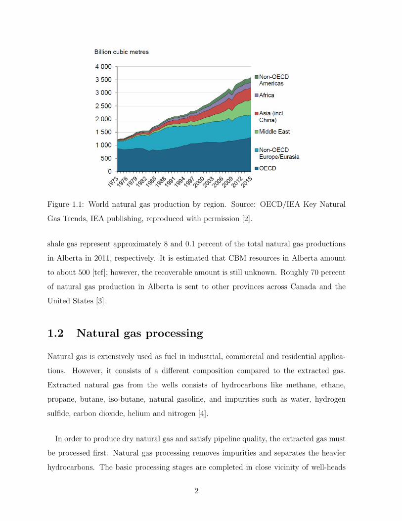
Figure 1.1: World natural gas production by region. Source: OECD/IEA Key Natural

Gas Trends, IEA publishing, reproduced with permission [2].

shale gas represent approximately 8 and 0.1 percent of the total natural gas productions

in Alberta in 2011, respectively. It is estimated that CBM resources in Alberta amount

to about 500 [tcf]; however, the recoverable amount is still unknown. Roughly 70 percent

of natural gas production in Alberta is sent to other provinces across Canada and the

United States [3].

1.2 Natural gas processing

Natural gas is extensively used as fuel in industrial, commercial and residential applica-

tions. However, it consists of a different composition compared to the extracted gas.

Extracted natural gas from the wells consists of hydrocarbons like methane, ethane,

propane, butane, iso-butane, natural gasoline, and impurities such as water, hydrogen

sulfide, carbon dioxide, helium and nitrogen [4].

In order to produce dry natural gas and satisfy pipeline quality, the extracted gas must

be processed first. Natural gas processing removes impurities and separates the heavier

hydrocarbons. The basic processing stages are completed in close vicinity of well-heads

2

!

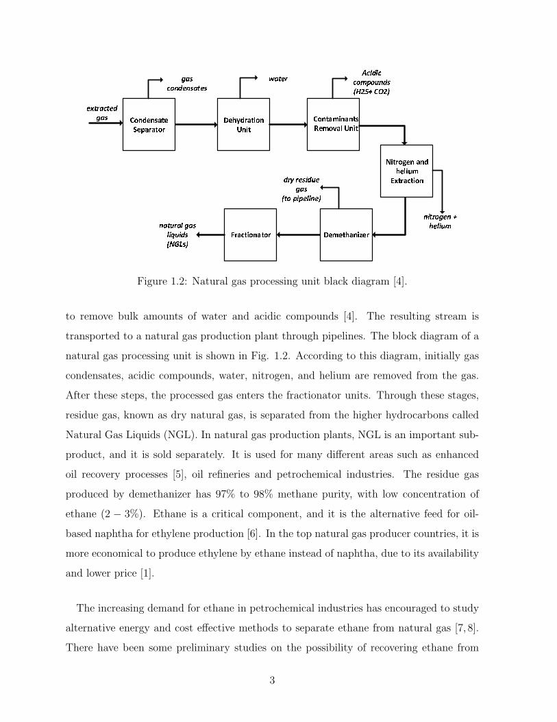
Figure 1.2: Natural gas processing unit black diagram [4].

to remove bulk amounts of water and acidic compounds [4]. The resulting stream is

transported to a natural gas production plant through pipelines. The block diagram of a

natural gas processing unit is shown in Fig. 1.2. According to this diagram, initially gas

condensates, acidic compounds, water, nitrogen, and helium are removed from the gas.

After these steps, the processed gas enters the fractionator units. Through these stages,

residue gas, known as dry natural gas, is separated from the higher hydrocarbons called

Natural Gas Liquids (NGL). In natural gas production plants, NGL is an important sub-

product, and it is sold separately. It is used for many different areas such as enhanced

oil recovery processes [5], oil refineries and petrochemical industries. The residue gas

produced by demethanizer has 97% to 98% methane purity, with low concentration of

ethane (2 − 3%). Ethane is a critical component, and it is the alternative feed for oil-

based naphtha for ethylene production [6]. In the top natural gas producer countries, it is

more economical to produce ethylene by ethane instead of naphtha, due to its availability

and lower price [1].

The increasing demand for ethane in petrochemical industries has encouraged to study

alternative energy and cost effective methods to separate ethane from natural gas [7, 8].

There have been some preliminary studies on the possibility of recovering ethane from

3

residue gas by adsorptive separations [9].

1.3 Adsorptive separation process

Cryogenic methods based on turbo expansion process at very low temperatures ∼ 188

K, are currently used to recover heavier hydrocarbons (NGLs) in natural gas processing

plants. Although cryogenic units have demonstrated high efficiencies, they are neither

energy nor cost efficient for medium and small applications. Adsorptive separation pro-

cesses are becoming widespread in various industries such as oil and gas as a promising

alternative. However, these processes have not been proven to be economically feasible.

Therefore, further studies are required in this area to achieve the maximum efficiency and

develop selective and durable materials.

As mentioned in the previous section, there are preliminary studies on ethane recovery

from natural gas using adsorptive separation processes. Perez et al. [9] studied the sep-

aration of ethane (C2) from residue gas using different adsorbents in a pressure/vacuum

swing adsorption (PVSA) cycle by multi-objective optimization. In general, adsorption is

governed by two different phenomena which take place simultaneously; equilibrium and

mass transfer. In order to optimize an adsorption unit, investigations in these two areas

are required. Malek and Farooq [10, 11] have performed dynamic column breakthrough

experiments to obtain equilibrium and kinetics data of ethane on activated carbon and

silica gel to develop a Pressure swing adsorption (PSA) simulation for hydrogen purifica-

tion. There are established and reliable techniques in the literature to measure adsorption

equilibrium [12]. Nevertheless, kinetics is more puzzling, due to its complexity and multi-

ple mechanisms that occur simultaneously. As a result, detailed knowledge of gas diffusion

within the porous media is needed for process design [13]. In order to study kinetics of

a system the first steps are to choose a reliable experimental technique and a suitable

mathematical model for correct measurements.

Mass transfer measurements by conventional uptake rate techniques are quite challeng-

ing. In these measurements, eliminating the external heat and mass transfers for strongly

4

adsorbed species are burdensome. In order to minimize these effects, one approach is to

use small amount of adsorbent; keeping in mind that sensitivity of equipment may cause

measurement limitations. In standard chromatographic measurements, external heat and

mass transfers are minimized by high velocity of gas stream. The major disadvantage

of this technique is the presence of axial dispersion in the system which affects the mass

transfer data [12]. Zero length column (ZLC) was first introduced in 1988 by Eic and

Ruthven [14] as a simple and rapid chromatographic technique to study adsorption kinet-

ics on small samples of zeolites with no dispersion effect. The mathematical model and

associated assumptions have been studied thoroughly ever since, in order to make ZLC

applicable for different systems.

1.4 Activated carbon

1.4.1 Applications

Several porous materials have been studied for ethane separation processes. All these sor-

bents have unique characteristics, such as high capacity, thermal stability, and mechanical

strength.

Activated carbons are among the most attractive porous materials used for adsorptive

separation processes, due to their ease of regeneration and high diffusivities. They are

known for their heterogeneous structure, randomly oriented pores, and wide pore size dis-

tribution compared to zeolites. Theses amorphous adsorbents generally show a polymodal

pore size distribution. Therefore, different mass transfer mechanisms are involved in gas

adsorption over these materials [15]. For this reason, adsorption kinetics in activated

carbons is an interesting topic from industrial and academic point of view. Although

there are several studies on adsorption of hydrocarbons over commercial adsorbents such

as activated carbon, the same sample from different manufacturing companies show var-

ious kinetics behaviors. This is due to difference in the production processes and pore

structure. This necessitates an independent study for every sample of activated carbon

produced by any individual manufacturer.

5

1.4.2 Production and characteristics

Activated carbon is a term used for a wide range of materials with carbon as the core

component. The common features of this group are their high porosity and high internal

surface area. The production process includes combustion or decomposition of organic

compounds with high carbon percentage. The first application of activated carbon was

many centuries ago when Egyptians used charcoals for medical and purification appli-

cations. The first industrial use goes back to 1900 in sugar refining industry [16]. Gas

adsorption by these carbonaceous materials gained attention during World War I, and

was utilized in gas masks to adsorb hazardous gases. Nowadays, there are numerous

types of activated carbons with versatile properties in different shapes such as granules,

finely divided powders, spherical, fibrous and cloth forms. They are used in waste water

treatments, air purifications, food processing and many more industries [16].

Activated carbons are composed of 85 to 95% carbon, whereas other elements such as

hydrogen, nitrogen, sulfur, and oxygen are also present. These atoms exist in the raw

materials, and transferred during the preparation procedure. Activated carbons are the

outcome of pyrolysis of raw materials which consists of two steps; carbonization at ∼

800C, and activation by CO2 or steam at ∼ 1000C. In the first step, decomposition

changes most of the noncarbon elements to volatile compounds, and others to aromatic

sheets which are cross-linked randomly. The random orientation of these sheets provides

free spaces that are filled with tar and other decomposition products. Activation clears

the interstices, and shapes randomly distributed pores with high surface areas. The pore

structure and adsorption characteristics of the carbonaceous material improves during the

second step [16].

The outcome is a substance with random arrangement of microcrystallites with porous

structures that are highly dependant on the raw materials and the production process.

The major portion of surface area in activated carbons is present in very small pores known

as micropores that have the effective diameters smaller than 2 nm. Pore classification

is based on the distance between the pore walls. Micropores often have comparable

6

dimensions to molecules. Generally, the specific micropore volume is 0.15 to 0.7 cm3

gin

activated carbons [13]. The surface area contributed by micropores account for roughly

95% of the total surface area. On the other hand, mesopores represent 5% of total surface

area. The effective dimension of this group is 2 to 50 nm [17], with specific volume of 0.1

to 0.2 cm3

g. Macropores are the last group in this classification, and they do not play a

significant role in the adsorption process. They are the channels for gas molecules to pass

through, and reach the mesopores and micropores [16]. There are different experimental

methods to characterize the pore structure in porous materials. Mercury porosimetry is

an effective method widely used for pore size distribution studies in the mesopores and

macropore range [18]. Gas adsorption is another technique usually applied in micropore

analysis [17]. These methods are covered in detail in Chapter 4.

As discussed above, the micropores provide the largest surface area and total volume in

activated carbons, and play the most important role in the adsorption process. However,

depending on the diffusing molecule radii, they may not enter the micropores. Similar

to porous structure, chemical composition of activated carbons has a strong influence on

adsorption properties. The non-carbon elements present in the activated carbon, such

as oxygen and hydrogen, are located on the edges and corners of the aromatic sheets.

The critical element is oxygen. Carbon-oxygen groups influence surface properties. As a

result, they increase the adsorption capacity in polar systems such as water [16].

1.5 Objective and organization of the present work

As mentioned earlier, adsorptive separation processes are gaining attention in industry as

an alternative technique for the conventional cryogenic processes. One of the proposed

applications of adsorptive processes is separating ethane from residue gas. A detailed

process design using pressure/vacuum swing adsorption on this topic has been completed

in our research group [19]. One of the candidate adsorbents for this separation is activated

carbon, due to its availability in the market. Hence, further investigation on adsorption of

ethane in activated carbon would help to design the optimized process with high efficiency.

7

The aim of this work is to study diffusion behavior of ethane at low concentrations

over activated carbon granules at temperatures between 303 and 373 K. In order to

achieve this, Zero Length Column measurements were conducted to study the controlling

mass transfer mechanism on different adsorbent sizes. Tortuosity factor is a property of

adsorbent describing the pore structure of solid. This parameter is also studied carefully

using the ZLC experimental results.

In this thesis, Chapter 2 reviews different mass transfer mechanisms present in adsorp-

tion, as well as related equations and the available measurement techniques. Zero Length

Column fundamentals, the mathematical model, and a summary of previous ZLC stud-

ies are discussed in Chapter 3. Chapter 4 is focused on practical aspects of the present

work such as experimental set-up, system characterization, experimental limitations, and

solid characterization techniques, mercury porosimetry and N2 adsorption measurements.

Chapter 5 is reserved for the main ZLC experimental results, model predictions, and fur-

ther discussions. Conclusion from the experimental results and recommended future work

are covered in the last chapter.

8

Chapter 2

Diffusion in Porous Solids:

Fundamentals and Measurement

Methods

Solids with porous structure can accommodate large amounts of gas or liquid. This

property has been utilized in several practical applications. Columns packed with these

materials (adsorbents) are commonly used for removing water traces from gas or liquid

streams [13]. The unique property of these materials is to selectively adsorb one com-

ponent from a mixture. The same processes are implemented in oil and gas refineries

to remove undesirable components. Removal of acidic compounds from natural gas can

be mentioned as a notable example. Another practical application is in purification pro-

cesses where increasing the purity of the valued component would result in economical

advantage, e.g. oxygen purification from air for medical practices [20].

The selectivity of an adsorbent depends on the differences in either adsorption kinetics

or adsorption equilibrium of the components involved in the separation [12]. As a result,

studies on these two governing phenomena for each component are important, and the

mechanisms should be understood carefully to model the separation behavior. The rate

of adsorption is usually controlled by the fluid transport through the packed columns and

inside the porous structure of the adsorbent, known as diffusion [21]. In this chapter,

9

different mechanisms of mass transfer in a porous solid are described, and a summary of

available diffusion measurement techniques is also provided. Activated carbons are one

category of the available adsorbents widely used in adsorptive processes, owing to their

thermal stability and high diffusivities. Previous studies on adsorption kinetics in acti-

vated carbons is reviewed in the last section.

2.1 Diffusion

Chemical potential gradient is the driving force for any mass transport phenomena. The

tendency of matter to eliminate chemical potetial variations in space and reach equilibrium

is called diffusion. Diffusion takes place in all the states of matter with different rates [21].

Adolf Fick is considered the first scientist to propose a mathematical formulation to define

diffusivity. He used the analogy of the Fourier heat conduction to model diffusion. Fick’s

first law of diffusion defines the term diffusivity resulting from concentration gradient in

isothermal conditions:

J = −D∂C∂x

(2.1)

In this mathematical representation, J is the mass flux, D is diffusivity, and ∂C∂x

is the

concentration gradient. Fick’s second law illustrates the concentration profile in a system

where diffusion is taking place [21]:

∂C

∂t= D

∂2C

∂x2(2.2)

Fick modeled the diffusing force in terms of concentration gradient, although it has been

since established in terms of the correct form should be that of the chemical potential

gradient. The simplification in using concentration gradient has consequences and are not

discussed here. Readers are referred to detailed literature on this topic [21]. Since this

thesis focuses on the diffusion of gases in solids only this topic will be discussed in detail.

10

2.2 Diffusion mechanisms

IUPAC classifies pores acording to their sizes [17]:

• pore sizes larger than ∼ 50 nm are called macropores;

• pore sizes between 2 nm and 50 nm are called mesopores;

• pores with sizes smaller than 2 nm are called micropores.

The diffusion mechanism depends on the pore size and the diameter of the diffusing

molecules. In the large pores transport is mainly dominated by the interactions between

the diffusing molecules, their collisions with the pore walls, and an additional flux due to

adsorbed species. However, in sufficiently small pores, when the pore diameter is compa-

rable with the molecular diameter, the molecules never escape from the force field of the

pore walls. There are several techniques to determine the dominant diffusion mechanisms.

Experiments should be conducted for each system to confirm the controlling diffusion

mechanism. This section describes different possible diffusion mechanisms present in the

porous materials.

2.2.1 Micropore diffusion

In micropores (pore sizes smaller than 2 nm), the pore diameter and the molecular diame-

ter of the diffusing species are typically within the same range. The transport of diffusing

molecules in these pore sizes is referred to as micropore diffusion. The practical applica-

tion of this is found in size-selective separations. If the size of one species in a mixture

is smaller than the micropore size of the adsorbent only that species will enter the pores.

In this range, surface forces play a significant role, diffusing molecules cannot escape this

strong force field, and they are considered as adsorbed phase. There are techniques avail-

able to measure micropore diffusivity, such as chromatography and NMR [12, 21] which

will be discussed in detail in the next section. When diffusion in the micropores controls

the rate of adsorption, the mathematical solution can be explained by Fick’s first law:

∂q

∂t=

1

r2∂

∂r(r2Dmicro

∂q

∂r) (2.3)

11

where q is the adsorbed phase concentration, r is radius vector, and Dmicro is micropore

diffusivity.

2.2.2 Macropore diffusion

If diffusion in micropores is quick enough, adsorption rate will be controlled by diffusion

through the macropores and mesopores of the particle. In this case, diffusion can be

controlled by four different mechanisms which are influenced by the pore size, system

conditions and adsorbate properties [12]. For instance, in large pores, interactions between

the diffusing molecules affect the transport rate. As pore size decreases collisions between

the diffusing species and the pore walls increase. This corresponds to Knudsen diffusion.

In small pores, contribution of surface diffusion becomes dominant. Total macropore

diffusivity is a function of all of the controlling mechanisms combined. Pore physical

properties, also, contribute to the total macropore diffusivity such as porosity and the

tortuosity. Tortuosity is a geometric factor which is an intrinsic characteristic of the

pores. It shows how pores deviate from an ideal cylindrical shape. Hences, it takes

into account the orientation of the pores and the different pore sizes in a particle [12].

Another term which is related to the pore characteristics is the porosity (εp) or void space

ratio in the solid particle. Both these terms can be measured using solid characterization

techniques. The measurement techniques and the contribution of pore properties will be

discussed in the next chapters.

The diffusivity and the equilibrium constant vary with temperature:

D = D0exp(−ERgT

) (2.4)

H = H0exp(−∆U0

RgT) (2.5)

In these equations, D0 and H0 are the pre-exponential constants, T is temperature, Rg

is the ideal gas constant, ∆U0 and E are heat of adsorption and activation energy which

are approximately within the same range. Activated diffusion mechanisms are discussed

12

in the subsequent sections.

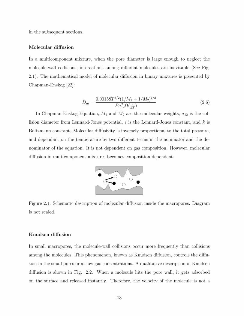
Molecular diffusion

In a multicomponent mixture, when the pore diameter is large enough to neglect the

molecule-wall collisions, interactions among different molecules are inevitable (See Fig.

2.1). The mathematical model of molecular diffusion in binary mixtures is presented by

Chapman-Enskog [22]:

Dm =0.00158T 3/2(1/M1 + 1/M2)

1/2

Pσ212Ω( ε

kT)

(2.6)

In Chapman-Enskog Equation, M1 and M2 are the molecular weights, σ12 is the col-

lision diameter from Lennard-Jones potential, ε is the Lennard-Jones constant, and k is

Boltzmann constant. Molecular diffusivity is inversely proportional to the total pressure,

and dependant on the temperature by two different terms in the nominator and the de-

nominator of the equation. It is not dependent on gas composition. However, molecular

diffusion in multicomponent mixtures becomes composition dependent.

Figure 2.1: Schematic description of molecular diffusion inside the macropores. Diagram

is not scaled.

Knudsen diffusion

In small macropores, the molecule-wall collisions occur more frequently than collisions

among the molecules. This phenomenon, known as Knudsen diffusion, controls the diffu-

sion in the small pores or at low gas concentrations. A qualitative description of Knudsen

diffusion is shown in Fig. 2.2. When a molecule hits the pore wall, it gets adsorbed

on the surface and released instantly. Therefore, the velocity of the molecule is not a

13

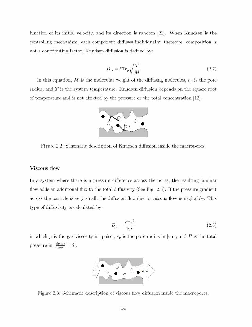
function of its initial velocity, and its direction is random [21]. When Knudsen is the

controlling mechanism, each component diffuses individually; therefore, composition is

not a contributing factor. Knudsen diffusion is defined by:

DK = 97rp

√T

M(2.7)

In this equation, M is the molecular weight of the diffusing molecules, rp is the pore

radius, and T is the system temperature. Knudsen diffusion depends on the square root

of temperature and is not affected by the pressure or the total concentration [12].

Figure 2.2: Schematic description of Knudsen diffusion inside the macropores.

Viscous flow

In a system where there is a pressure difference across the pores, the resulting laminar

flow adds an additional flux to the total diffusivity (See Fig. 2.3). If the pressure gradient

across the particle is very small, the diffusion flux due to viscous flow is negligible. This

type of diffusivity is calculated by:

Dv =Prp

2

8µ(2.8)

in which µ is the gas viscosity in [poise], rp is the pore radius in [cm], and P is the total

pressure in [dynescm2 ] [12].

Figure 2.3: Schematic description of viscous flow diffusion inside the macropores.

14

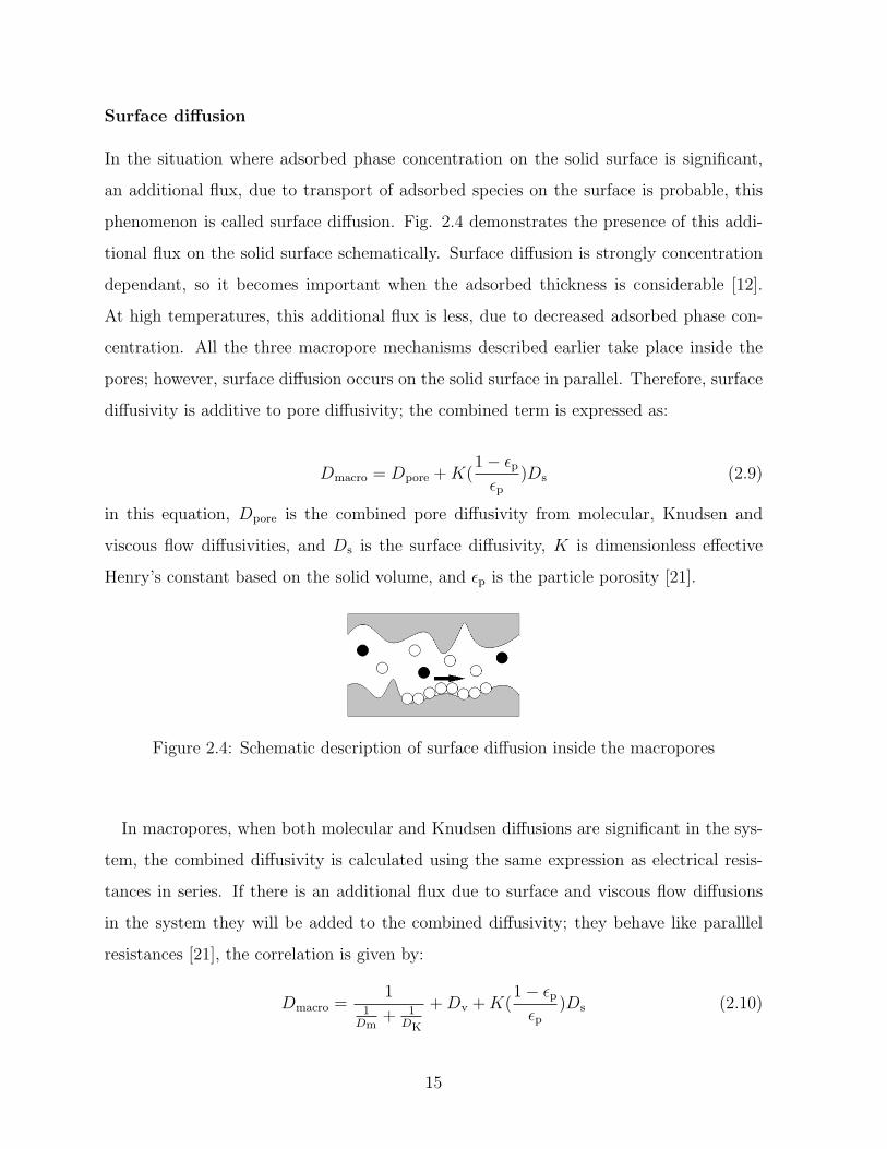
Surface diffusion

In the situation where adsorbed phase concentration on the solid surface is significant,

an additional flux, due to transport of adsorbed species on the surface is probable, this

phenomenon is called surface diffusion. Fig. 2.4 demonstrates the presence of this addi-

tional flux on the solid surface schematically. Surface diffusion is strongly concentration

dependant, so it becomes important when the adsorbed thickness is considerable [12].

At high temperatures, this additional flux is less, due to decreased adsorbed phase con-

centration. All the three macropore mechanisms described earlier take place inside the

pores; however, surface diffusion occurs on the solid surface in parallel. Therefore, surface

diffusivity is additive to pore diffusivity; the combined term is expressed as:

Dmacro = Dpore +K(1 − εpεp

)Ds (2.9)

in this equation, Dpore is the combined pore diffusivity from molecular, Knudsen and

viscous flow diffusivities, and Ds is the surface diffusivity, K is dimensionless effective

Henry’s constant based on the solid volume, and εp is the particle porosity [21].

Figure 2.4: Schematic description of surface diffusion inside the macropores

In macropores, when both molecular and Knudsen diffusions are significant in the sys-

tem, the combined diffusivity is calculated using the same expression as electrical resis-

tances in series. If there is an additional flux due to surface and viscous flow diffusions

in the system they will be added to the combined diffusivity; they behave like paralllel

resistances [21], the correlation is given by:

Dmacro =1

1Dm

+ 1DK

+Dv +K(1 − εpεp

)Ds (2.10)

15

2.3 Mass transfer resistances

The adsorption of a component is usually described by two transport mechanisms; trans-

port through the gas medium to the surface of the adsorbent, and transport into the

particle known as diffusion. The combination of these mechanisms control the rate of

adsorption. Transport inside the porous particles was discussed in the previous section,

the particle is typically surrounded by a laminar layer, and mass transfer occurs from this

sub-layer to the particle surface by molecular diffusion. Film resistance can be defined by

the linear driving force (LDF) equation:

∂q

∂t=

3kfRp

(C − C∗) (2.11)

In this equation, q is the average adsorbed phase concentration over the particle, Rp

is the particle radius, C is the concentration of the diffusing molecules, and C∗ is the fluid

phase concentration that would be at equilibrium with the adsorbed phase. Mass transfer

coefficient introduces a dimensionless parameter called Sherwood number (Sh) which is

defined by:

Sh =2kfRp

Dm

(2.12)

This number in the analogous to Nusselt number (Nu) in heat transfer studies. In the

static conditions Sherwood number is equal to 2.0. It increases with an increase in the

flow. The sherwood number is related to Reynolds (Re) and Schmidt (Sc) numbers

which are the dimensionless parameters characterizing the flow conditions [21]. There

are several correlations that show the relationship between these three parameters in

solid-fluid systems as found in the literature [22]. One such correlation is [12]:

Sh = 2.0 + 1.1Sc13Re0.6 (2.13)

Transport inside the pores is typically slower than transport through the external fluid

film. As a result, the fluid film usually has a minor contribution in the total resistance

16

as compared to pore diffusion mechanisms. If more than one resistance control the mass

transfer in the system, the effective mass transfer coefficient k is defined as [12]:

1

kH=

rc2

15HDmicro

+Rp

2

15εpDmacro

+Rp

3kf(2.14)

In this equation, H is equilibrium constant, rc is micro-particle radius, and Rp is particle

radius.

2.4 Experimental techniques

There are several available techniques to study diffusion in porous materials. This section

contains a brief review of the traditional methods used for studying adsorption kinetics.

2.4.1 Uptake rate measurements

One of the techniques commonly used for determining the intraparticle diffusivity is batch

experiment. In this technique, a number of particles are placed in the apparatus, and are

exposed to a step change in sorbate concentration at the external surface of the particle

at time zero. The rate of adsorption is measured by following the mass of the adsorbent

(gravimetry) or the pressure in the chamber (volumetry). The diffusional time constant

can be calculated by comparing the experimental results to the analytical solution. The

particles used in the experiment can be either adsorbent crystals or pellets. This mea-

surement requires a very sensitive balance or pressure transducers for reliable results [12].

Although straightforward this technique has a few shortcomings. The use of large mass

of the solid leads to strong heat effects that can mask the measurement of mass transfer.

2.4.2 Chromatographic methods

The external heat and mass transfers cannot be perfectly eliminated in the batch exper-

iments. Chromatographic methods are the alternative to the conventional uptake rate

measurements. In these methods, a gas stream flows through a column packed with the

17

adsorbent particles. Chromatographic measurements are performed by a step change or

pulse injection to a packed column, or a reduced amount of adsorbent particles, called

differential beds. Dispersion may be present in such systems. In order to separate the

dispersion and mass transfer effects, experiments over a range of gas velocities should be

performed [12].

One of the chromatographic techniques in which experiments are carried out on a small

amount of adsorbent under high flow rates of gas is Zero Length Column (ZLC) [14].

It was developed to study intraparticle diffusivities by eliminating the dispersion effect

which is present in other chromatographic techniques [21]. Zero Length Column is the

method used for diffusion measurements in the present study and will be discussed in the

following chapter.

2.4.3 NMR spectroscopy

Nuclear magnetic resonance (NMR) spectroscopy is an analytical technique widely used

in organic chemistry to detect the unknown species in complex solutions. This technique

was developed based on the interactions between the diffusing molecules in an external

magnetic field. It is also used in characterising atoms and molecules in order to determine

the diffusivity and solubility. This method is a powerful technique for diffusion measure-

ments such as elementary processes in the molecular level. Self diffusion measurements

is another application where the molecules under study are labeled and experiments are

performed under equilibrium condition [21]. However, this technique is more suitable in

molecular and self diffusivity determination.

2.5 Diffusion in activated carbon

Activated carbons are widely used in adsorptive separation processes [23]. They are

commercially available in large amounts, and they possess unique properties relevant to

these processes, such as high internal surface area, thermal staibility and high diffusion

rates [24]. According to their pore analysis, they have randomly ordered pore network

18

with wide pore size distributions, due to their production procedure [13]. They exhibit

bimodal distributions, comprising microporous structure throughout a network of larger

macropores. Therefore, diffusion in such systems is more complex than similar systems

[21]. As mentioned earlier, adsorption of gas on adsorbent particles is controlled by various

mass transfer resistances; transport to the particle surface and diffusion into the particle.

Film resistance can be determined by the relevant equations available in the literature [22].

On the other hand, the rate of diffusion of the gas in the adsorbent particle should be

measured and calculated for each system with the aid of mathematical models [25].

Gas diffusion in the macropores is usually due to molecular and Knudsen diffusions. In

activated carbons, it is possible for gas molecules to adsorb significantly on the surface.

This adds an additional flux in parallel to that of the pore diffusion, and accelerates

the transfer [26]. This mechanism is known as surface diffusion, and is significant at

high adsorbed concentrations. Doong et al. [27] studied PSA separation of a mixture

of CO2, H2, and CH4, and noticed that surface diffusion contributed 50% of the total

flux over the activated carbon sample. Do et al. [28] perfromed differntial adsorption

bed (DAB) experiments of ethane in activated carbon. They proposed a model based

on pore and surface diffusion in the system. They could successfully verify the model by

the DAB results. Unlike pore diffusion, surface diffusion is concentration dependant; i.e.

adsorbed molecules become more mobile in higher concentrations. There are available

models that describe the concentration dependence of surface diffusion of different species

on activated carbons [29, 30]. The classical theories used for surface diffusion cannot be

applied for activatd carbon. Mesured surface diffusivities in activated carbons have been

shown faster behavior. This behavior is due to the disordered distribution of pores in

their structure [31]. Hu et al. [32] performed DAB experiments of ethane and propane

in Ajax activated carbon differentially in order to study the concentration dependence of

surface diffusion. They observed that at higher surface coverages, the traditional theories

fail to explain high surface diffusivities in activated carbons. Micropore diffusion was also

predicted and observed by the previous studies in the small and medium size particles

of activated carbon. Hu and Do [33], developed a mathematical model for adsorption of

19

hydrocarbons in small particles of activated carbons. They showed that ethane adsorption

on activated carbons is not only controlled by macropore diffusion but also micropore

diffusion, and the combination of pore and surface diffusions cannot fully predict the

uptake rate results.

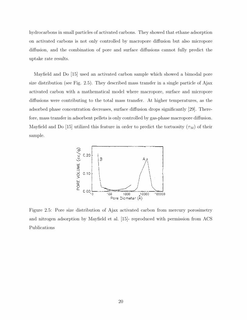
Mayfield and Do [15] used an activated carbon sample which showed a bimodal pore

size distribution (see Fig. 2.5). They described mass transfer in a single particle of Ajax

activated carbon with a mathematical model where macropore, surface and micropore

diffusions were contributing to the total mass transfer. At higher temperatures, as the

adsorbed phase concentration decreases, surface diffusion drops significantly [29]. There-

fore, mass transfer in adsorbent pellets is only controlled by gas-phase macropore diffusion.

Mayfield and Do [15] utilized this feature in order to predict the tortuosity (τM) of their

sample.

Figure 2.5: Pore size distribution of Ajax activated carbon from mercury porosimetry

and nitrogen adsorption by Mayfield et al. [15]- reproduced with permission from ACS

Publications

20

Chapter 3

Zero Length Column Technique

Zero length column (ZLC) is one of the available techniques to study diffusion. It

was first introduced by Eic and Ruthven to measure intracystalline diffusivity in zeolite

powders [14]. Over these years, the method has been extended and modified to measure

diffusion in pellets, liquid systems, bi-porous materials, and to study equilibrium. The

advantage of this approach lies in the elimination of external heat and mass transfer resis-

tances by using small amount of adsorbent, low concentration of sorbate in gas, and high

flow rates of purge gas. In comparison with the conventional chromatographic methods,

ZLC is simple and fast which makes it a suitable candidate for lab-scale adsorption kinet-

ics studies or rapid screenings [34,35]. The diffusion measurements reported in this thesis

were all performed using ZLC technique. This chapter is focused on ZLC background,

theory and the previous studies on this topic.

3.1 Theory of ZLC

In ZLC, the column is packed with a small amount of the adsorbent (∼ 5 mg). The

sample is first pre-equilibrated with the test gas. Then, a switching valve is used to

switch the gas stream from the test to a non adsorbing purge gas, typically helium.

Kinetics and equilibrium characteristics of the system are measured by following the

desorption behavior of the adsorbate. The mathematical model used to describe the ZLC

21

system, is based on the Fick’s second law of diffusion describing the mass balance in the

particles [21]. In addition, mass balance of the adsorbing component in the fluid phase

is, also, considered. These two mass balances have to be solved simultaneously, to derive

the desorption curve. In this model it is assumed that system is at isothermal conditions,

particles are spherical, and ZLC column is a well mixed cell [14]. It is worth noting that

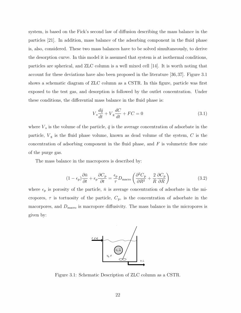
account for these deviations have also been proposed in the literature [36,37]. Figure 3.1

shows a schematic diagram of ZLC column as a CSTR. In this figure, particle was first

exposed to the test gas, and desorption is followed by the outlet concentration. Under

these conditions, the differential mass balance in the fluid phase is:

V sdq

dt+ V g

dC

dt+ FC = 0 (3.1)

where V s is the volume of the particle, q is the average concentration of adsorbate in the

particle, V g is the fluid phase volume, known as dead volume of the system, C is the

concentration of adsorbing component in the fluid phase, and F is volumetric flow rate

of the purge gas.

The mass balance in the macropores is described by:

(1 − εp)∂n

∂t+ εp

∂Cp

∂t=εpτDmacro

(∂2Cp

∂R2+

2

R

∂Cp

∂R

)(3.2)

where εp is porosity of the particle, n is average concentration of adsorbate in the mi-

cropores, τ is tortuosity of the particle, Cp, is the concentration of adsorbate in the

macorpores, and Dmacro is macropore diffusivity. The mass balance in the micropores is

given by:

Figure 3.1: Schematic Description of ZLC column as a CSTR.

22

∂n

∂t= Dmicro

(∂2n

∂r2+

2

r

∂n

∂r

)(3.3)

∂n

∂t=

3

rcDmicro

∂n

∂r

∣∣r=rc

(3.4)

∂q

∂t=

3

Rp

εpτDmacro

∂Cp

∂R

∣∣R=Rp

(3.5)

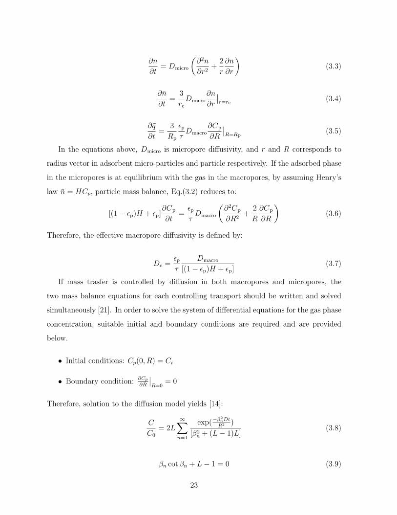
In the equations above, Dmicro is micropore diffusivity, and r and R corresponds to

radius vector in adsorbent micro-particles and particle respectively. If the adsorbed phase

in the micropores is at equilibrium with the gas in the macropores, by assuming Henry’s

law n = HCp, particle mass balance, Eq.(3.2) reduces to:

[(1 − εp)H + εp]∂Cp

∂t=εpτDmacro

(∂2Cp

∂R2+

2

R

∂Cp

∂R

)(3.6)

Therefore, the effective macropore diffusivity is defined by:

De =εpτ

Dmacro

[(1 − εp)H + εp](3.7)

If mass trasfer is controlled by diffusion in both macropores and micropores, the

two mass balance equations for each controlling transport should be written and solved

simultaneously [21]. In order to solve the system of differential equations for the gas phase

concentration, suitable initial and boundary conditions are required and are provided

below.

• Initial conditions: Cp(0, R) = Ci

• Boundary condition: ∂Cp

∂R

∣∣R=0

= 0

Therefore, solution to the diffusion model yields [14]:

C

C0

= 2L∞∑n=1

exp(−β2nDtR2 )

[β2n + (L− 1)L]

(3.8)

βn cot βn + L− 1 = 0 (3.9)

23

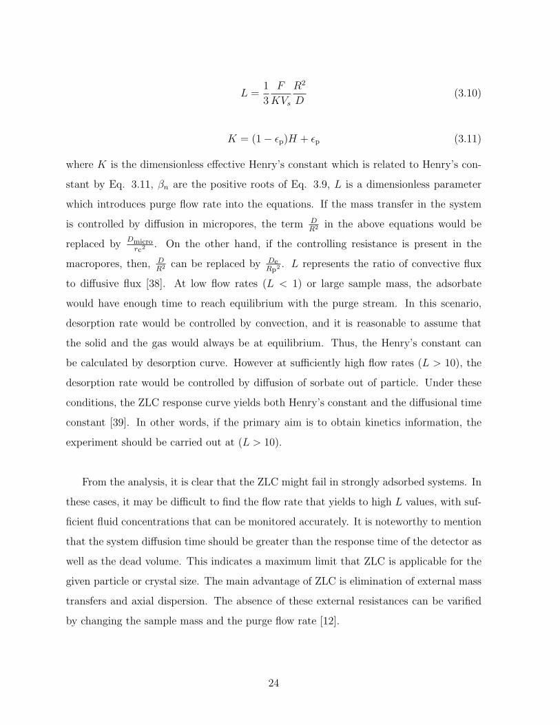
L =1

3

F

KVs

R2

D(3.10)

K = (1 − εp)H + εp (3.11)

where K is the dimensionless effective Henry’s constant which is related to Henry’s con-

stant by Eq. 3.11, βn are the positive roots of Eq. 3.9, L is a dimensionless parameter

which introduces purge flow rate into the equations. If the mass transfer in the system

is controlled by diffusion in micropores, the term DR2 in the above equations would be

replaced byDmicrorc2

. On the other hand, if the controlling resistance is present in the

macropores, then, DR2 can be replaced by De

Rp2 . L represents the ratio of convective flux

to diffusive flux [38]. At low flow rates (L < 1) or large sample mass, the adsorbate

would have enough time to reach equilibrium with the purge stream. In this scenario,

desorption rate would be controlled by convection, and it is reasonable to assume that

the solid and the gas would always be at equilibrium. Thus, the Henry’s constant can

be calculated by desorption curve. However at sufficiently high flow rates (L > 10), the

desorption rate would be controlled by diffusion of sorbate out of particle. Under these

conditions, the ZLC response curve yields both Henry’s constant and the diffusional time

constant [39]. In other words, if the primary aim is to obtain kinetics information, the

experiment should be carried out at (L > 10).

From the analysis, it is clear that the ZLC might fail in strongly adsorbed systems. In

these cases, it may be difficult to find the flow rate that yields to high L values, with suf-

ficient fluid concentrations that can be monitored accurately. It is noteworthy to mention

that the system diffusion time should be greater than the response time of the detector as

well as the dead volume. This indicates a maximum limit that ZLC is applicable for the

given particle or crystal size. The main advantage of ZLC is elimination of external mass

transfers and axial dispersion. The absence of these external resistances can be varified

by changing the sample mass and the purge flow rate [12].

24

3.2 Long time asymptote analysis

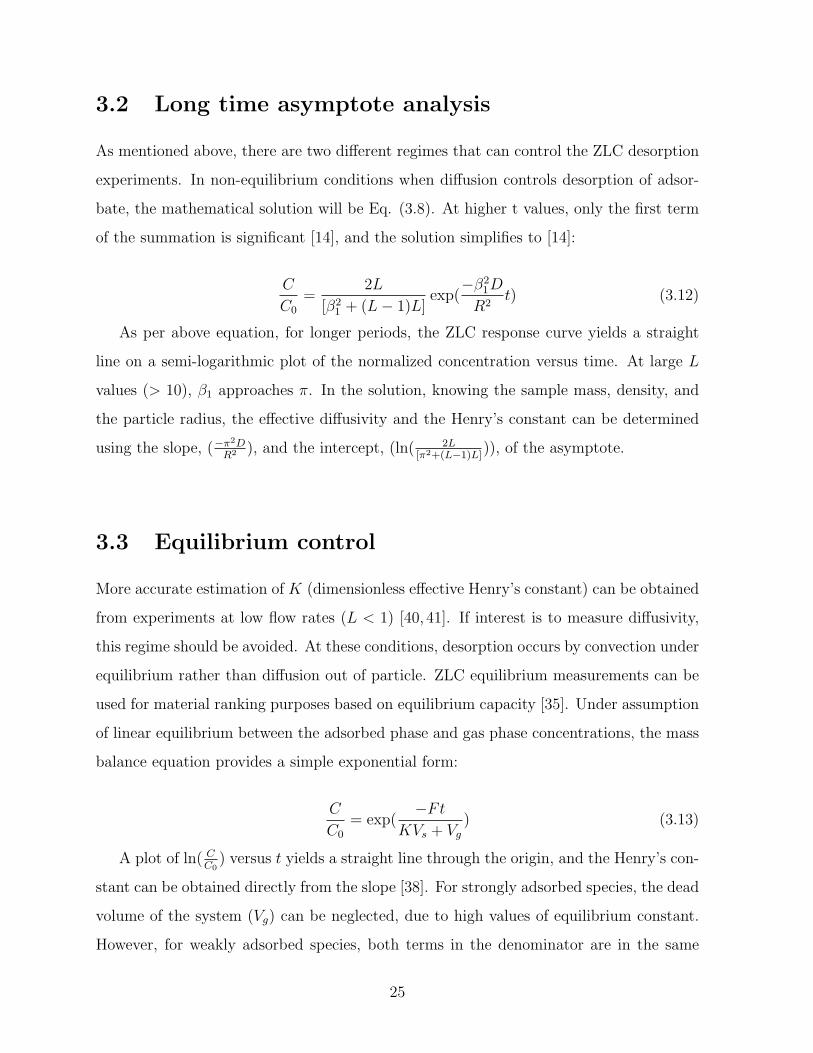
As mentioned above, there are two different regimes that can control the ZLC desorption

experiments. In non-equilibrium conditions when diffusion controls desorption of adsor-

bate, the mathematical solution will be Eq. (3.8). At higher t values, only the first term

of the summation is significant [14], and the solution simplifies to [14]:

C

C0

=2L

[β21 + (L− 1)L]

exp(−β2

1D

R2t) (3.12)

As per above equation, for longer periods, the ZLC response curve yields a straight

line on a semi-logarithmic plot of the normalized concentration versus time. At large L

values (> 10), β1 approaches π. In the solution, knowing the sample mass, density, and

the particle radius, the effective diffusivity and the Henry’s constant can be determined

using the slope, (−π2DR2 ), and the intercept, (ln( 2L

[π2+(L−1)L])), of the asymptote.

3.3 Equilibrium control

More accurate estimation of K (dimensionless effective Henry’s constant) can be obtained

from experiments at low flow rates (L < 1) [40, 41]. If interest is to measure diffusivity,

this regime should be avoided. At these conditions, desorption occurs by convection under

equilibrium rather than diffusion out of particle. ZLC equilibrium measurements can be

used for material ranking purposes based on equilibrium capacity [35]. Under assumption

of linear equilibrium between the adsorbed phase and gas phase concentrations, the mass

balance equation provides a simple exponential form:

C

C0

= exp(−Ft

KVs + Vg) (3.13)

A plot of ln( CC0

) versus t yields a straight line through the origin, and the Henry’s con-

stant can be obtained directly from the slope [38]. For strongly adsorbed species, the dead

volume of the system (Vg) can be neglected, due to high values of equilibrium constant.

However, for weakly adsorbed species, both terms in the denominator are in the same

25

order of magnitude. In this case, Vg can be easily measured by the same ZLC experiment

with an empty column. The area under the ZLC blank response curve provides the dead

volume of the system. In an equilibrium controlled system, the ZLC desorption curve in

the plot of CC0

versus Ft (Flow × time) only depends on the desorption volume [39]. This

indicates that the curves at different flow rates should overlap. On the other hand, in a

kinetically controlled system, curves would diverage. An increase in the flow rate results

a decrease in the fluid phase concentration. There is a point at which ZLC response for

higher flow rate crosses the lower flow rate response. These are the simple experimental

checks to confirm whether experiments are performed under equilibrium or the kinetically

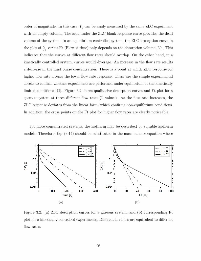
limited conditions [42]. Figure 3.2 shows qualitative desorption curves and Ft plot for a

gaseous system at three different flow rates (L values). As the flow rate increases, the

ZLC response deviates from the linear form, which confirms non-equilibrium conditions.

In addition, the cross points on the Ft plot for higher flow rates are clearly noticeable.

For more concentrated systems, the isotherm may be described by suitable isotherm

models. Therefore, Eq. (3.14) should be substituted in the mass balance equation where

(a) (b)

Figure 3.2: (a) ZLC desorption curves for a gaseous system, and (b) corresponding Ft

plot for a kinetically controlled experiments. Different L values are equivalent to different

flow rates.

26

dqdC

is calculated by the isotherm model. For a system modelled by Langmuir isotherm, the

solution of the ZLC desorption curve under equilibrium conditions will be characterized

as Eq. (3.15) [38].

dq

dt=

dq

dC.dC

dt(3.14)

ln(C

C0

) =−Ft

KVs + Vg− KVsKVs + Vg

[1

1 + bC− 1

1 + bC0

+ ln(1 + bC0

1 + bC)

](3.15)

This solution reduces to a linear response at very low concentrations.

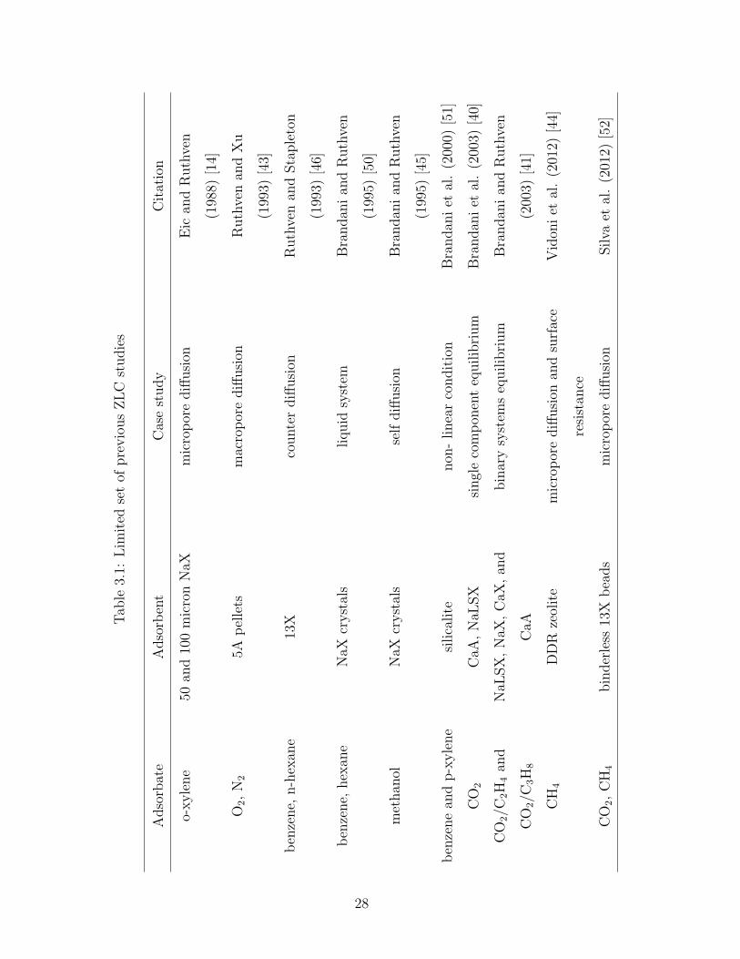
3.4 Previous studies using ZLC

Since the time ZLC was introduced to determine diffusivity of gases in microporous solids

[14], it has been applied to several systems, in order to measure and obtain the controlling

diffusion mechanims: intracrystalline (micropore) diffusion, macropore diffusion [39, 43],

and surface resistance [44]. Through the time, the method has been changed and modified

to study self diffusivity [45], counter diffusion [46], kinetics in liquid systems [46]. These

modifications change the traditional ZLC to be applicable under non-linear conditions [47],

non-isothermal systems [48], biporous adsorbents [49]. In addition, Brandani et al. [40,41]

modified the ZLC assumptions to measure equilibrium for single components and binary

systems which was explained in detail in the previous section. Table 3.1 lists some of

previous works on ZLC and case studies.

27

Tab

le3.

1:L

imit

edse

tof

pre

vio

us

ZL

Cst

udie

s

Adso

rbat

eA

dso

rben

tC

ase

study

Cit

atio

n

o-xyle

ne

50an

d10

0m

icro

nN

aXm

icro

por

ediff

usi

onE

ican

dR

uth

ven

(198

8)[1

4]

O2,

N2

5Ap

elle

tsm

acro

por

ediff

usi

onR

uth

ven

and

Xu

(199

3)[4

3]

ben

zene,

n-h

exan

e13

Xco

unte

rdiff

usi

onR

uth

ven

and

Sta

ple

ton

(199

3)[4

6]

ben

zene,

hex

ane

NaX

cryst

als

liquid

syst

emB

randan

ian

dR

uth

ven

(199

5)[5

0]

met

han

olN

aXcr

yst

als

self

diff

usi

onB

randan

ian

dR

uth

ven

(199

5)[4

5]

ben

zene

and

p-x

yle

ne

silica

lite

non

-linea

rco

ndit

ion

Bra

ndan

iet

al.

(200

0)[5

1]

CO

2C

aA,

NaL

SX

singl

eco

mp

onen

teq

uilib

rium

Bra

ndan

iet

al.

(200

3)[4

0]

CO

2/C

2H

4an

d

CO

2/C

3H

8

NaL

SX

,N

aX,

CaX

,an

d

CaA

bin

ary

syst

ems

equilib

rium

Bra

ndan

ian

dR

uth

ven

(200

3)[4

1]

CH

4D

DR

zeol

ite

mic

rop

ore

diff

usi

onan

dsu

rfac

e

resi

stan

ce

Vid

oni

etal

.(2

012)

[44]

CO

2,

CH

4bin

der

less

13X

bea

ds

mic

rop

ore

diff

usi

onSilva

etal

.(2

012)

[52]

28

Chapter 4

Experimental Procedure and Solid

Characterization

In the previous chapter, we discussed that the ZLC technique was modified to study

kinetics and equilibrium in different systems. The mathematical model based on Fick’s

law of diffusion was provided. In this chapter, details of the ZLC experiments such as

experimental set-up and procedure, choice of detector, data processing method, dead

volume measurements, and solid characterization experiments are discussed.

4.1 ZLC set-up

During this project, a ZLC set-up was developed to study diffusion in porous solids. Some

preliminary tests on the set-up and the solid were conducted prior to the ZLC experi-

ments, such as dead volume determination and solid characterization. These aspects will

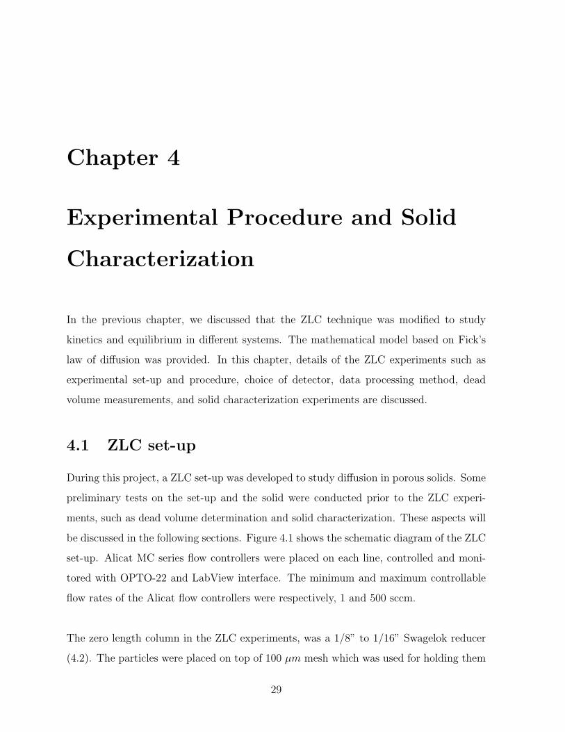
be discussed in the following sections. Figure 4.1 shows the schematic diagram of the ZLC

set-up. Alicat MC series flow controllers were placed on each line, controlled and moni-

tored with OPTO-22 and LabView interface. The minimum and maximum controllable

flow rates of the Alicat flow controllers were respectively, 1 and 500 sccm.

The zero length column in the ZLC experiments, was a 1/8” to 1/16” Swagelok reducer

(4.2). The particles were placed on top of 100 µm mesh which was used for holding them

29

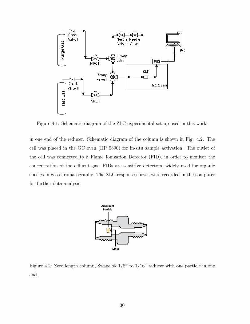
Figure 4.1: Schematic diagram of the ZLC experimental set-up used in this work.

in one end of the reducer. Schematic diagram of the column is shown in Fig. 4.2. The

cell was placed in the GC oven (HP 5890) for in-situ sample activation. The outlet of

the cell was connected to a Flame Ionization Detector (FID), in order to monitor the

concentration of the effluent gas. FIDs are sensitive detectors, widely used for organic

species in gas chromatography. The ZLC response curves were recorded in the computer

for further data analysis.

Figure 4.2: Zero length column, Swagelok 1/8” to 1/16” reducer with one particle in one

end.

30

In all the experiments, 2-GA activated carbon obtained from Kuraray corporation was

used. Prior to the experiments, the sample was activated at 200C for a particle of ∼ 4

mg at the flow rate of 5 sccm. The test was dry dilute ethane, 1% ethane mixed with

helium, as provided by Praxair. In the experiments both He (purity of 99.5%) and N2

(purity of 99.5%) provided by the same company was used as the purge gas.

4.2 ZLC procedure

The ZLC experiments were started by regenerating the adsorbent by subjecting it to high

temperature. After activation, the system temperature was reduced to the experimental

temperature (30, 50 or 70C), and the sample was pre-equilibrated with the test gas (he-

lium stream containing 1% ethane) for a period of 1 hour. At time zero, the flow was

switched to pure purge gas (He or N2) at the same flow rate. In order to have a smooth

transition when switching the valve, a vent line was added to the purge line prior to the

main switch valve. Two needle valves were installed on the vent line to maintain the

system pressure at a constant value. The FID signal was continuously monitored by com-

puter, and then converted to normalized concentration. The ZLC tests were performed

at different flow rates ranging from 5 to 50 sccm, and were repeated to ensure data re-

producibility.

4.3 Choice of detector

ZLC experiments require a sensitive detector to monitor the concentration of the sorbate

in the gas stream. In order to find the best detector for the system under study, pre-

liminary tests on different detectors namely, Flame Ionization Detector (FID), Thermal

Conductivity Detector (TCD), Mass Spectrometer (MS) were studied and tested for ac-

curacy, sensitivity, ease of calibration and dead volume.

31

Flame ionization detector (FID)

Flame ionization detectors are widely used in organic gas chromatography and are well-

known for their sensitivity. In this type of detector, the gas passes through a hydrogen/air

flame, and combustion of the gas in the flame produces ions. The generation of the ions

is proportional to the concentration of organic species in the gas stream. The main dis-

advantage of FID is its failure to detect inorganic compounds. However, the advantages

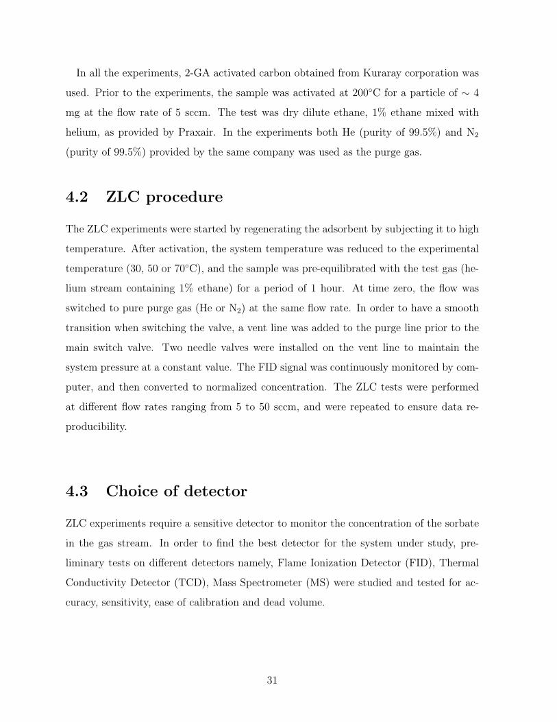
prevail for organic systems due to its linear response and high sensitivity of about 10-7.

The detector Linearity was verified using different mixtures of ethane in helium by FID

connected to a HP 9800 GC. These mixtures were prepared by metering the flows of

helium and ethane. According to the results provided in Fig. 4.3, FID passes sensitivity

and calibration tests even at very low concentrations of ethane.

(a) (b)

Figure 4.3: Flame ionization detector calibration curves at (a) high and (b) low concen-

trations.

Thermal Conductivity Detector

The Thermal conductivity detector (TCD) measures the thermal conductivity of the gas

and compares it with a reference gas (i.e. He or H2). The most significant advantage of

this equipment is its ability to detect both the organic and inorganic compounds. Pre-

32

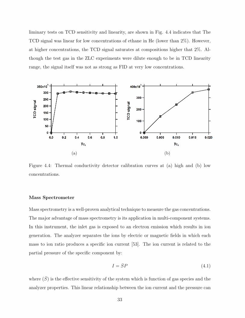
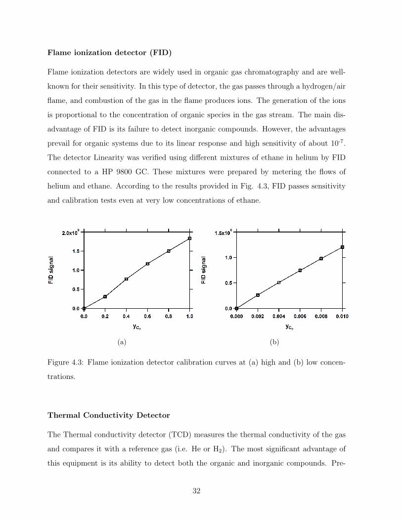
liminary tests on TCD sensitivity and linearity, are shown in Fig. 4.4 indicates that The

TCD signal was linear for low concentrations of ethane in He (lower than 2%). However,

at higher concentrations, the TCD signal saturates at compositions higher that 2%. Al-

though the test gas in the ZLC experiments were dilute enough to be in TCD linearity

range, the signal itself was not as strong as FID at very low concentrations.

(a) (b)

Figure 4.4: Thermal conductivity detector calibration curves at (a) high and (b) low

concentrations.

Mass Spectrometer

Mass spectrometry is a well-proven analytical technique to measure the gas concentrations.

The major advantage of mass spectrometry is its application in multi-component systems.

In this instrument, the inlet gas is exposed to an electron emission which results in ion

generation. The analyzer separates the ions by electric or magnetic fields in which each

mass to ion ratio produces a specific ion current [53]. The ion current is related to the

partial pressure of the specific component by:

I = SP (4.1)

where (S) is the effective sensitivity of the system which is function of gas species and the

analyzer properties. This linear relationship between the ion current and the pressure can

33

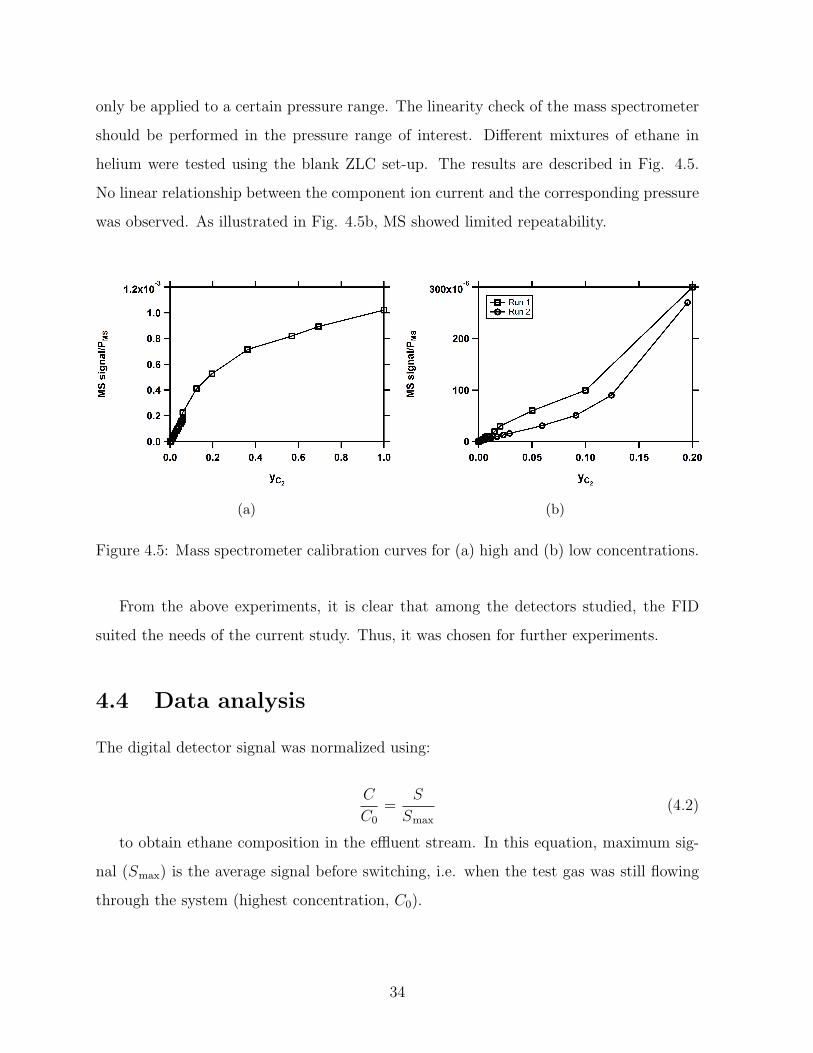
only be applied to a certain pressure range. The linearity check of the mass spectrometer

should be performed in the pressure range of interest. Different mixtures of ethane in

helium were tested using the blank ZLC set-up. The results are described in Fig. 4.5.

No linear relationship between the component ion current and the corresponding pressure

was observed. As illustrated in Fig. 4.5b, MS showed limited repeatability.

(a) (b)

Figure 4.5: Mass spectrometer calibration curves for (a) high and (b) low concentrations.

From the above experiments, it is clear that among the detectors studied, the FID

suited the needs of the current study. Thus, it was chosen for further experiments.

4.4 Data analysis

The digital detector signal was normalized using:

C

C0

=S

Smax

(4.2)

to obtain ethane composition in the effluent stream. In this equation, maximum sig-

nal (Smax) is the average signal before switching, i.e. when the test gas was still flowing

through the system (highest concentration, C0).

34

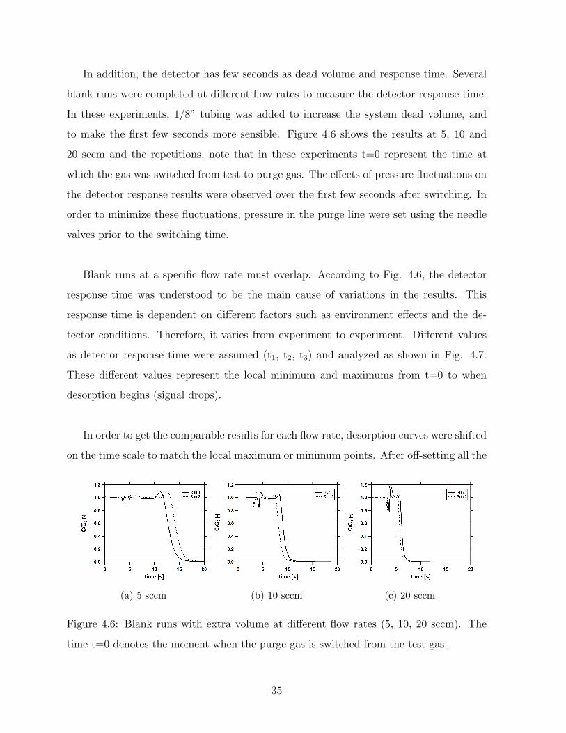
In addition, the detector has few seconds as dead volume and response time. Several

blank runs were completed at different flow rates to measure the detector response time.

In these experiments, 1/8” tubing was added to increase the system dead volume, and

to make the first few seconds more sensible. Figure 4.6 shows the results at 5, 10 and

20 sccm and the repetitions, note that in these experiments t=0 represent the time at

which the gas was switched from test to purge gas. The effects of pressure fluctuations on

the detector response results were observed over the first few seconds after switching. In

order to minimize these fluctuations, pressure in the purge line were set using the needle

valves prior to the switching time.

Blank runs at a specific flow rate must overlap. According to Fig. 4.6, the detector

response time was understood to be the main cause of variations in the results. This

response time is dependent on different factors such as environment effects and the de-

tector conditions. Therefore, it varies from experiment to experiment. Different values

as detector response time were assumed (t1, t2, t3) and analyzed as shown in Fig. 4.7.

These different values represent the local minimum and maximums from t=0 to when

desorption begins (signal drops).

In order to get the comparable results for each flow rate, desorption curves were shifted

on the time scale to match the local maximum or minimum points. After off-setting all the

(a) 5 sccm (b) 10 sccm (c) 20 sccm

Figure 4.6: Blank runs with extra volume at different flow rates (5, 10, 20 sccm). The

time t=0 denotes the moment when the purge gas is switched from the test gas.

35

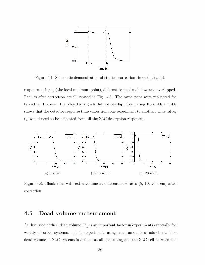
Figure 4.7: Schematic demonstration of studied correction times (t1, t2, t3).

responses using t1 (the local minimum point), different tests of each flow rate overlapped.

Results after correction are illustrated in Fig. 4.8. The same steps were replicated for

t2 and t3. However, the off-setted signals did not overlap. Comparing Figs. 4.6 and 4.8

shows that the detector response time varies from one experiment to another. This value,

t1, would need to be off-setted from all the ZLC desorption responses.

(a) 5 sccm (b) 10 sccm (c) 20 sccm

Figure 4.8: Blank runs with extra volume at different flow rates (5, 10, 20 sccm) after

correction.

4.5 Dead volume measurement

As discussed earlier, dead volume, V g is an important factor in experiments especially for

weakly adsorbed systems, and for experiments using small amounts of adsorbent. The

dead volume in ZLC systems is defined as all the tubing and the ZLC cell between the

36

switching valve and the detector. In order to measure the system dead volume, blank

tests have to be carried out using an empty ZLC column. The area under desorption

response curve in Ft plot corresponds to the system dead volume. This value should be

subtracted from all the ZLC responses to avoid errors in analysis. Figure 4.9 shows the

ZLC blank experiments performed at different flow rates (5-50 sccm). In these experi-

ments, 1% ethane in helium is the test gas, and pure He is used as the purge gas. The

total measured dead volume of the ZLC set-up is ∼ 0.5 cc. It is also observed that the

time required for CC0

to reach a value of 0.0001 at flow rate of 50 sccm is ∼ 20 seconds.

Figure 4.9: Blank ZLC responses at different flow rates.

4.6 Isotherm measurement

The adsorption isotherms were measured using high pressure adsorption analyzer (HPVA-

100) from VIT scientific instruments. This volumetric system contained a dosing cell and

a sample cell with known volumes (V dose and V sample respectively). There are a number

of pressure transducers and sensitive thermocouples installed in each of these cells that

monitor pressure and temperature data. First, an adsorbent sample with a known mass

was loaded in the sample cell. This cell was then evacuated and out-gassed. Meanwhile,

the dosing cell filled with the test gas. A known volume of the test gas was transferred

from the dosing cell to the sample cell through the tubing and the valves. System dead

37

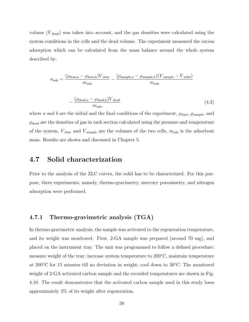
volume (V dead) was taken into account, and the gas densities were calculated using the

system conditions in the cells and the dead volume. The experiment measured the excess

adsorption which can be calculated from the mass balance around the whole system

described by:

nads =(ρdose,a − ρdose,b)V dose

mads

− (ρsample,a − ρsample,b)(V sample − V solid)

mads

− (ρdead,a − ρdead,b)V dead

mads

(4.3)

where a and b are the initial and the final conditions of the experiment, ρdose, ρsample, and

ρdead are the densities of gas in each section calculated using the pressure and temperature

of the system, V dose and V sample are the volumes of the two cells, mads is the adsorbent

mass. Results are shown and discussed in Chapter 5.

4.7 Solid characterization

Prior to the analysis of the ZLC curves, the solid has to be characterized. For this pur-

pose, three experiments, namely, thermo-gravimetry, mercury porosimetry, and nitrogen

adsorption were performed.

4.7.1 Thermo-gravimetric analysis (TGA)

In thermo-gravimetric analysis, the sample was activated to the regeneration temperature,

and its weight was monitored. First, 2-GA sample was prepared (around 70 mg), and

placed on the instrument tray. The unit was programmed to follow a defined procedure:

measure weight of the tray; increase system temperature to 200C, maintain temperature

at 200C for 15 minutes till no deviation in weight; cool down to 30C. The monitored

weight of 2-GA activated carbon sample and the recorded temperatures are shown in Fig.

4.10. The result demonstrates that the activated carbon sample used in this study loses

approximately 3% of its weight after regeneration.

38

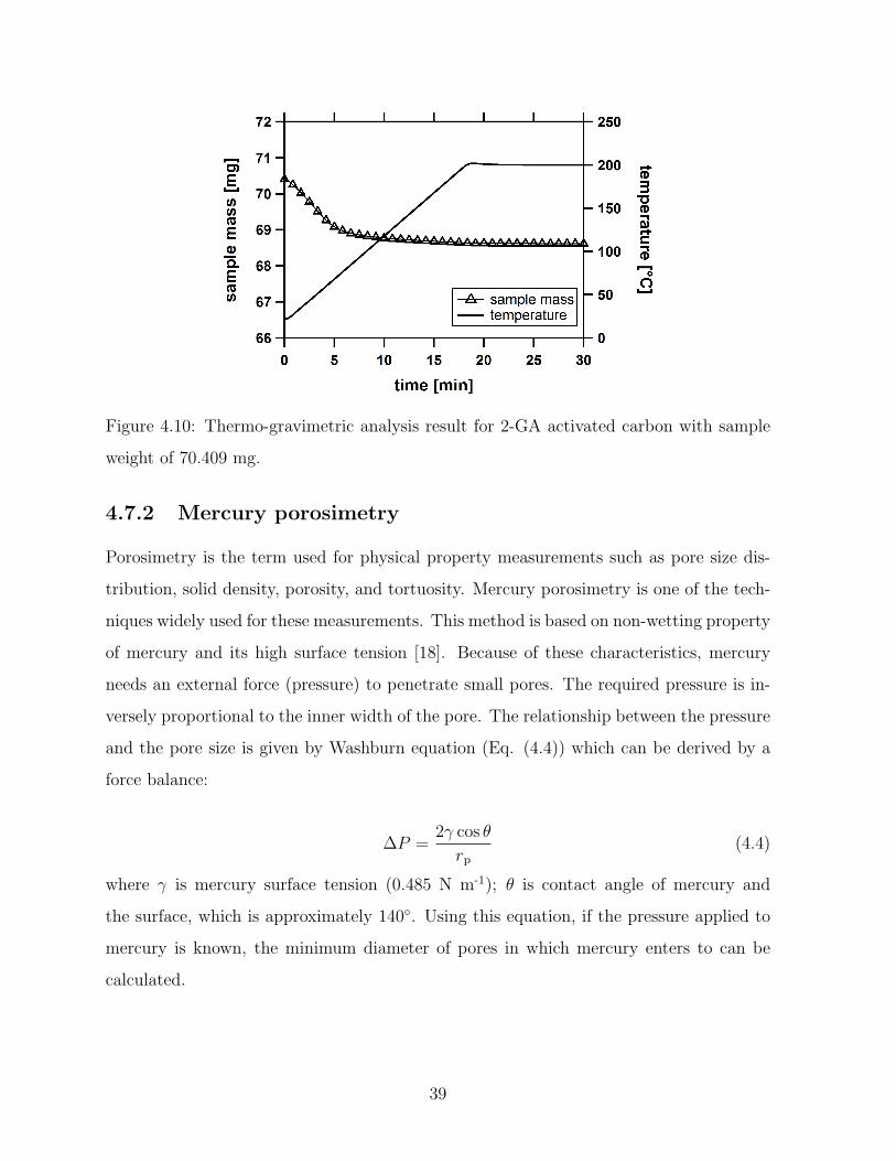
Figure 4.10: Thermo-gravimetric analysis result for 2-GA activated carbon with sample

weight of 70.409 mg.

4.7.2 Mercury porosimetry

Porosimetry is the term used for physical property measurements such as pore size dis-

tribution, solid density, porosity, and tortuosity. Mercury porosimetry is one of the tech-

niques widely used for these measurements. This method is based on non-wetting property

of mercury and its high surface tension [18]. Because of these characteristics, mercury

needs an external force (pressure) to penetrate small pores. The required pressure is in-

versely proportional to the inner width of the pore. The relationship between the pressure

and the pore size is given by Washburn equation (Eq. (4.4)) which can be derived by a

force balance:

∆P =2γ cos θ

rp(4.4)

where γ is mercury surface tension (0.485 N m-1); θ is contact angle of mercury and

the surface, which is approximately 140. Using this equation, if the pressure applied to

mercury is known, the minimum diameter of pores in which mercury enters to can be

calculated.

39

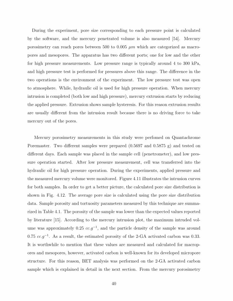
During the experiment, pore size corresponding to each pressure point is calculated

by the software, and the mercury penetrated volume is also measured [54]. Mercury

porosimetry can reach pores between 500 to 0.005 µm which are categorized as macro-

pores and mesopores. The apparatus has two different ports; one for low and the other

for high pressure measurements. Low pressure range is typically around 4 to 300 kPa,

and high pressure test is performed for pressures above this range. The difference in the

two operations is the environment of the experiment. The low pressure test was open

to atmosphere. While, hydraulic oil is used for high pressure operation. When mercury

intrusion is completed (both low and high pressure), mercury extrusion starts by reducing

the applied pressure. Extrusion shows sample hysteresis. For this reason extrusion results

are usually different from the intrusion result because there is no driving force to take

mercury out of the pores.

Mercury porosimetry measurements in this study were perfomed on Quantachrome

Poremaster. Two different samples were prepared (0.5697 and 0.5875 g) and tested on

different days. Each sample was placed in the sample cell (penetrometer), and low pres-

sure operation started. After low pressure measurement, cell was transferred into the

hydraulic oil for high pressure operation. During the experiments, applied pressure and

the measured mercury volume were monitored. Figure 4.11 illustrates the intrusion curves

for both samples. In order to get a better picture, the calculated pore size distribution is

shown in Fig. 4.12. The average pore size is calculated using the pore size distribution

data. Sample porosity and tortuosity parameters measured by this technique are summa-

rized in Table 4.1. The porosity of the sample was lower than the expected values reported

by literature [15]. According to the mercury intrusion plot, the maximum intruded vol-

ume was approximately 0.25 cc.g−1, and the particle density of the sample was around

0.75 cc.g−1. As a result, the estimated porosity of the 2-GA activated carbon was 0.33.

It is worthwhile to mention that these values are measured and calculated for macrop-

ores and mesopores, however, activated carbon is well-known for its developed micropore

structure. For this reason, BET analysis was performed on the 2-GA activated carbon

sample which is explained in detail in the next section. From the mercury porosimetry

40

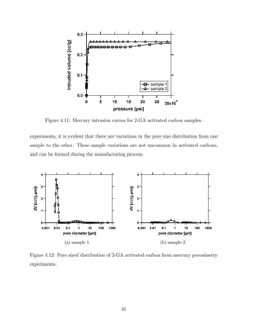
Figure 4.11: Mercury intrusion curves for 2-GA activated carbon samples.

experiments, it is evident that there are variations in the pore size distribution from one

sample to the other. These sample variations are not uncommon in activated carbons,

and can be formed during the manufacturing process.

(a) sample 1 (b) sample 2

Figure 4.12: Pore sized distribution of 2-GA activated carbon from mercury porosimetry

experiments.

41

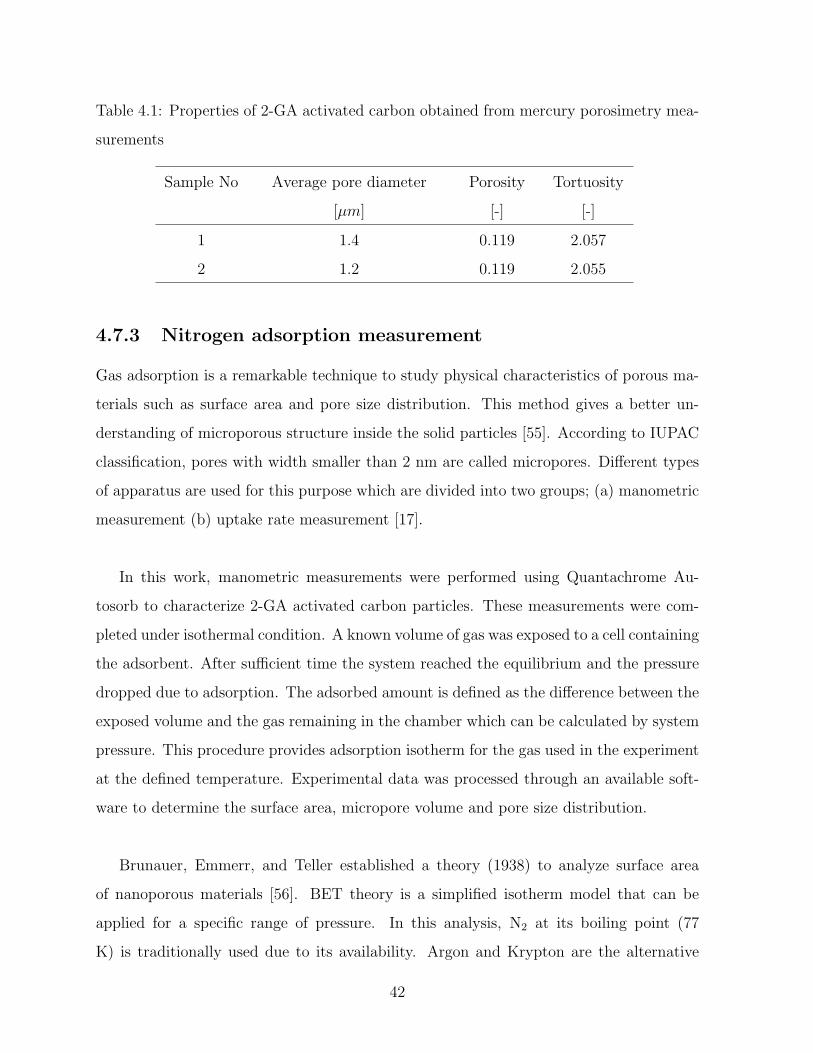
Table 4.1: Properties of 2-GA activated carbon obtained from mercury porosimetry mea-

surements

Sample No Average pore diameter Porosity Tortuosity

[µm] [-] [-]

1 1.4 0.119 2.057

2 1.2 0.119 2.055

4.7.3 Nitrogen adsorption measurement

Gas adsorption is a remarkable technique to study physical characteristics of porous ma-

terials such as surface area and pore size distribution. This method gives a better un-

derstanding of microporous structure inside the solid particles [55]. According to IUPAC

classification, pores with width smaller than 2 nm are called micropores. Different types

of apparatus are used for this purpose which are divided into two groups; (a) manometric

measurement (b) uptake rate measurement [17].

In this work, manometric measurements were performed using Quantachrome Au-

tosorb to characterize 2-GA activated carbon particles. These measurements were com-

pleted under isothermal condition. A known volume of gas was exposed to a cell containing

the adsorbent. After sufficient time the system reached the equilibrium and the pressure

dropped due to adsorption. The adsorbed amount is defined as the difference between the

exposed volume and the gas remaining in the chamber which can be calculated by system

pressure. This procedure provides adsorption isotherm for the gas used in the experiment

at the defined temperature. Experimental data was processed through an available soft-

ware to determine the surface area, micropore volume and pore size distribution.

Brunauer, Emmerr, and Teller established a theory (1938) to analyze surface area

of nanoporous materials [56]. BET theory is a simplified isotherm model that can be

applied for a specific range of pressure. In this analysis, N2 at its boiling point (77

K) is traditionally used due to its availability. Argon and Krypton are the alternative

42

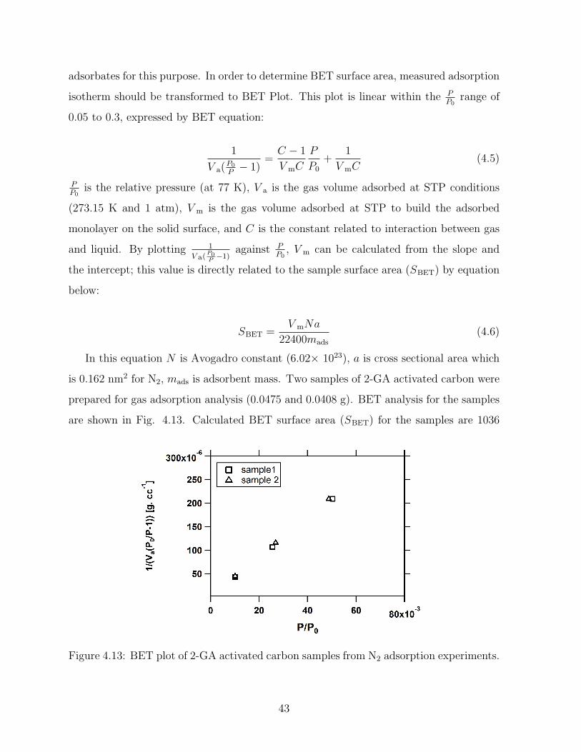
adsorbates for this purpose. In order to determine BET surface area, measured adsorption

isotherm should be transformed to BET Plot. This plot is linear within the PP0

range of

0.05 to 0.3, expressed by BET equation:

1

V a(P0

P− 1)

=C − 1

V mC

P

P0

+1

V mC(4.5)

PP0

is the relative pressure (at 77 K), V a is the gas volume adsorbed at STP conditions

(273.15 K and 1 atm), V m is the gas volume adsorbed at STP to build the adsorbed

monolayer on the solid surface, and C is the constant related to interaction between gas

and liquid. By plotting 1

V a(P0P−1)

against PP0

, V m can be calculated from the slope and

the intercept; this value is directly related to the sample surface area (SBET) by equation

below:

SBET =V mNa

22400mads

(4.6)

In this equation N is Avogadro constant (6.02× 1023), a is cross sectional area which

is 0.162 nm2 for N2, mads is adsorbent mass. Two samples of 2-GA activated carbon were

prepared for gas adsorption analysis (0.0475 and 0.0408 g). BET analysis for the samples

are shown in Fig. 4.13. Calculated BET surface area (SBET) for the samples are 1036

Figure 4.13: BET plot of 2-GA activated carbon samples from N2 adsorption experiments.

43

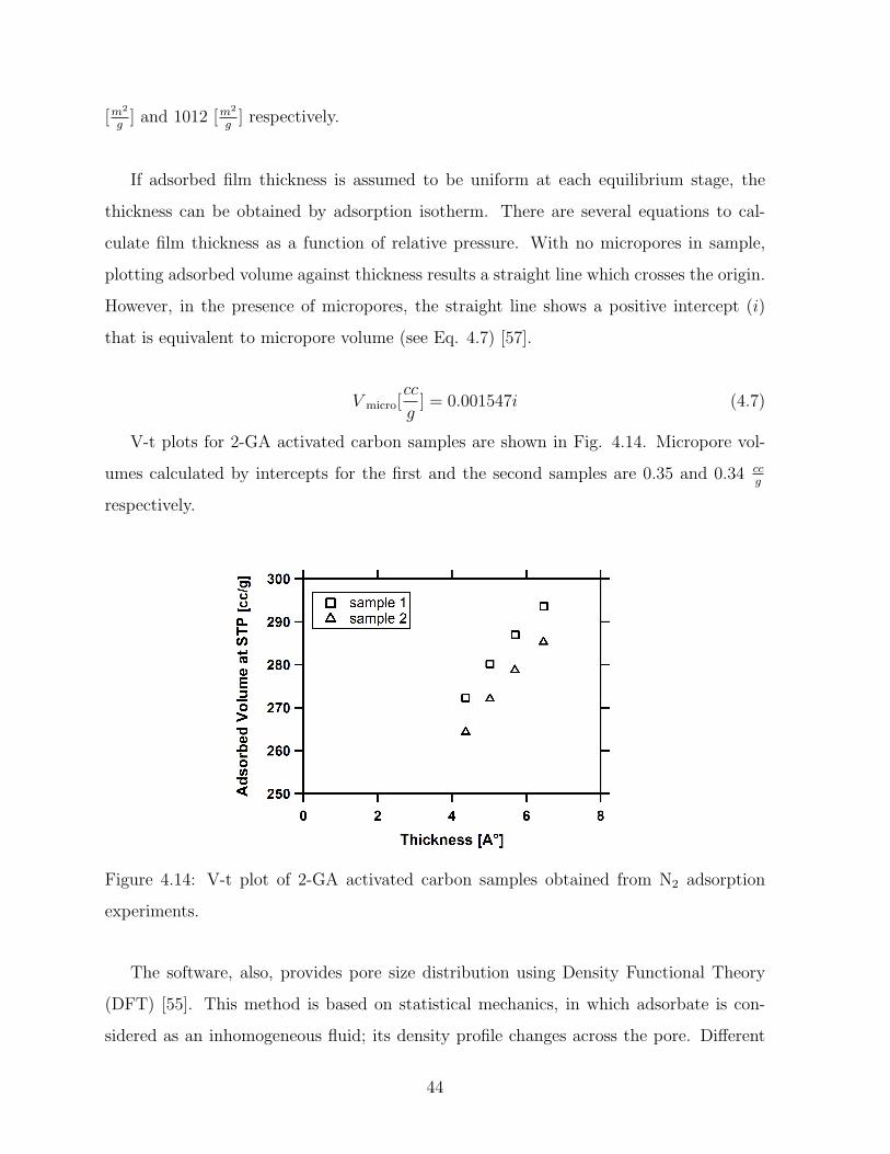
[m2

g] and 1012 [m

2

g] respectively.

If adsorbed film thickness is assumed to be uniform at each equilibrium stage, the

thickness can be obtained by adsorption isotherm. There are several equations to cal-

culate film thickness as a function of relative pressure. With no micropores in sample,

plotting adsorbed volume against thickness results a straight line which crosses the origin.

However, in the presence of micropores, the straight line shows a positive intercept (i)

that is equivalent to micropore volume (see Eq. 4.7) [57].

V micro[cc

g] = 0.001547i (4.7)

V-t plots for 2-GA activated carbon samples are shown in Fig. 4.14. Micropore vol-

umes calculated by intercepts for the first and the second samples are 0.35 and 0.34 ccg

respectively.

Figure 4.14: V-t plot of 2-GA activated carbon samples obtained from N2 adsorption

experiments.

The software, also, provides pore size distribution using Density Functional Theory

(DFT) [55]. This method is based on statistical mechanics, in which adsorbate is con-

sidered as an inhomogeneous fluid; its density profile changes across the pore. Different

44

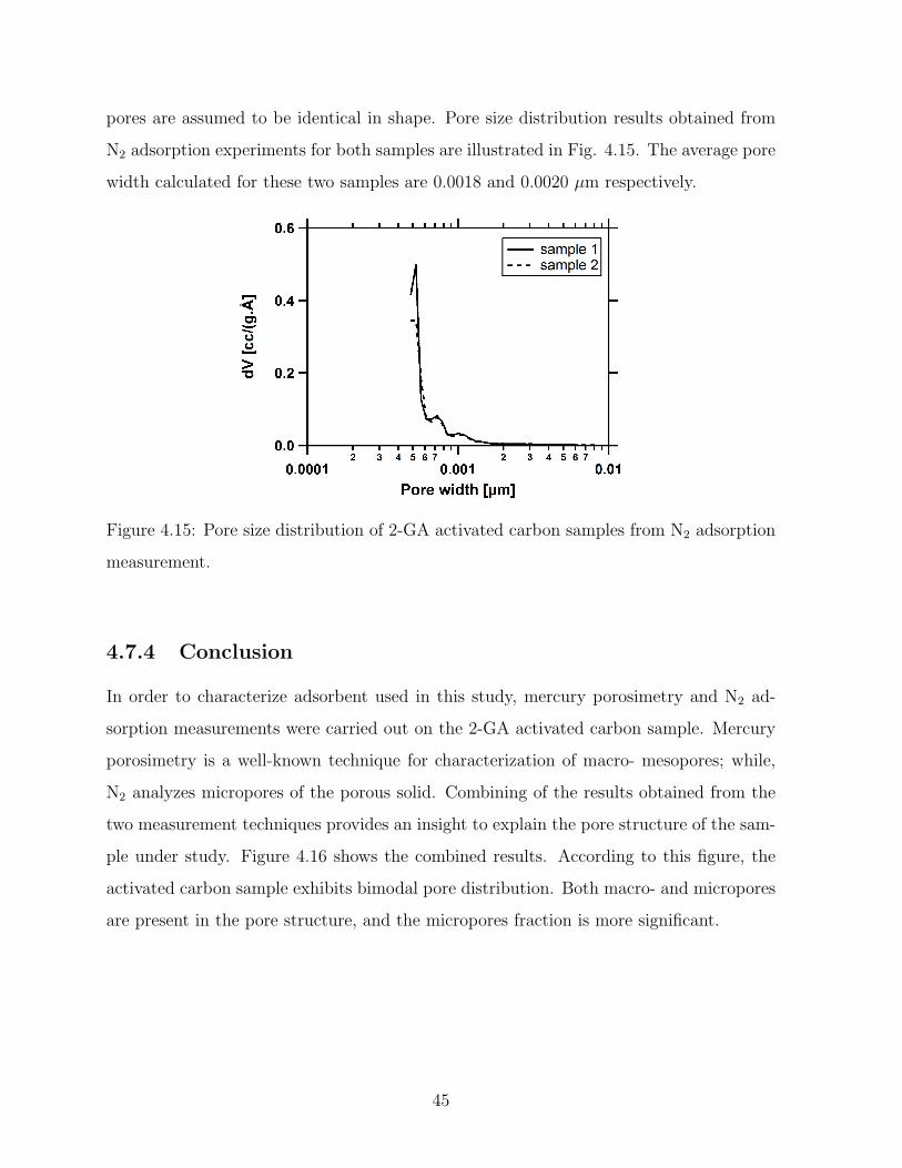
pores are assumed to be identical in shape. Pore size distribution results obtained from

N2 adsorption experiments for both samples are illustrated in Fig. 4.15. The average pore

width calculated for these two samples are 0.0018 and 0.0020 µm respectively.

Figure 4.15: Pore size distribution of 2-GA activated carbon samples from N2 adsorption

measurement.

4.7.4 Conclusion

In order to characterize adsorbent used in this study, mercury porosimetry and N2 ad-

sorption measurements were carried out on the 2-GA activated carbon sample. Mercury

porosimetry is a well-known technique for characterization of macro- mesopores; while,

N2 analyzes micropores of the porous solid. Combining of the results obtained from the

two measurement techniques provides an insight to explain the pore structure of the sam-

ple under study. Figure 4.16 shows the combined results. According to this figure, the

activated carbon sample exhibits bimodal pore distribution. Both macro- and micropores

are present in the pore structure, and the micropores fraction is more significant.

45

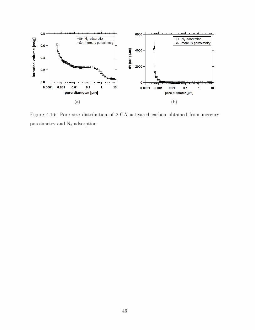
(a) (b)

Figure 4.16: Pore size distribution of 2-GA activated carbon obtained from mercury

porosimetry and N2 adsorption.

46

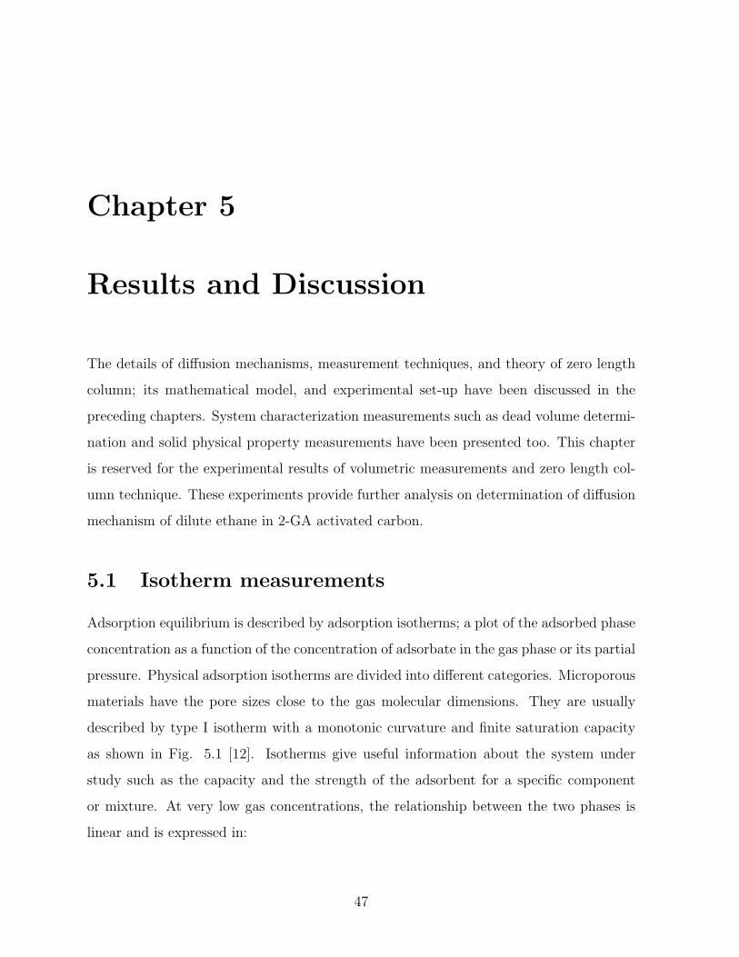
Chapter 5

Results and Discussion

The details of diffusion mechanisms, measurement techniques, and theory of zero length

column; its mathematical model, and experimental set-up have been discussed in the

preceding chapters. System characterization measurements such as dead volume determi-

nation and solid physical property measurements have been presented too. This chapter

is reserved for the experimental results of volumetric measurements and zero length col-

umn technique. These experiments provide further analysis on determination of diffusion

mechanism of dilute ethane in 2-GA activated carbon.

5.1 Isotherm measurements

Adsorption equilibrium is described by adsorption isotherms; a plot of the adsorbed phase

concentration as a function of the concentration of adsorbate in the gas phase or its partial

pressure. Physical adsorption isotherms are divided into different categories. Microporous

materials have the pore sizes close to the gas molecular dimensions. They are usually

described by type I isotherm with a monotonic curvature and finite saturation capacity

as shown in Fig. 5.1 [12]. Isotherms give useful information about the system under

study such as the capacity and the strength of the adsorbent for a specific component

or mixture. At very low gas concentrations, the relationship between the two phases is

linear and is expressed in:

47

Figure 5.1: Qualitative description of type I isotherm and Henry’s law constant.

q = HC (5.1)

where q is the concentration of the adsorbed phase and C is the concentration of adsorbate

in the gas phase. This condition is known as Henry’s Law and the slope is called Henry’s

Law constant (see Fig. 5.1). At higher concentrations, isotherms deviate from the linear

form and become curved [38]. There are different mathematical models that predict the

behavior of adsorption isotherms by a number of parameters. The Langmuir isotherm is

perhaps the simplest model which is commonly used to describe adsorption equilibrium

as shown below:

q =qsbC

1 + bC(5.2)

In the above equation, qs, b, and C are saturation capacity, affinity parameter, and fluid

phase concentration, respectively. The affinity parameter (b) is described by

b = b0exp(−∆U

RgT) (5.3)

where b0 is the pre-exponential factor, ∆U is the the internal energy of adsorption, T is

temperature, and Rg is the ideal gas constant. In this model, it is assumed that adsorption

on the surface is a monolayer, each site can accommodate only one adsorbed molecule,

different sites are energetically homogeneous, and there is no interaction between the

48

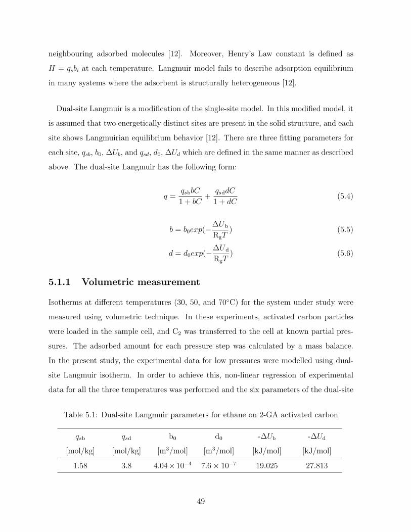
neighbouring adsorbed molecules [12]. Moreover, Henry’s Law constant is defined as

H = qsbi at each temperature. Langmuir model fails to describe adsorption equilibrium

in many systems where the adsorbent is structurally heterogeneous [12].

Dual-site Langmuir is a modification of the single-site model. In this modified model, it

is assumed that two energetically distinct sites are present in the solid structure, and each

site shows Langmuirian equilibrium behavior [12]. There are three fitting parameters for

each site, qsb, b0, ∆Ub, and qsd, d0, ∆Ud which are defined in the same manner as described

above. The dual-site Langmuir has the following form:

q =qsbbC

1 + bC+

qsddC

1 + dC(5.4)

b = b0exp(−∆Ub

RgT) (5.5)

d = d0exp(−∆Ud

RgT) (5.6)

5.1.1 Volumetric measurement

Isotherms at different temperatures (30, 50, and 70C) for the system under study were

measured using volumetric technique. In these experiments, activated carbon particles

were loaded in the sample cell, and C2 was transferred to the cell at known partial pres-

sures. The adsorbed amount for each pressure step was calculated by a mass balance.

In the present study, the experimental data for low pressures were modelled using dual-

site Langmuir isotherm. In order to achieve this, non-linear regression of experimental

data for all the three temperatures was performed and the six parameters of the dual-site

Table 5.1: Dual-site Langmuir parameters for ethane on 2-GA activated carbon

qsb

[mol/kg]

qsd

[mol/kg]

b0

[m3/mol]

d0

[m3/mol]

-∆Ub

[kJ/mol]

-∆Ud

[kJ/mol]

1.58 3.8 4.04× 10−4 7.6 × 10−7 19.025 27.813

49

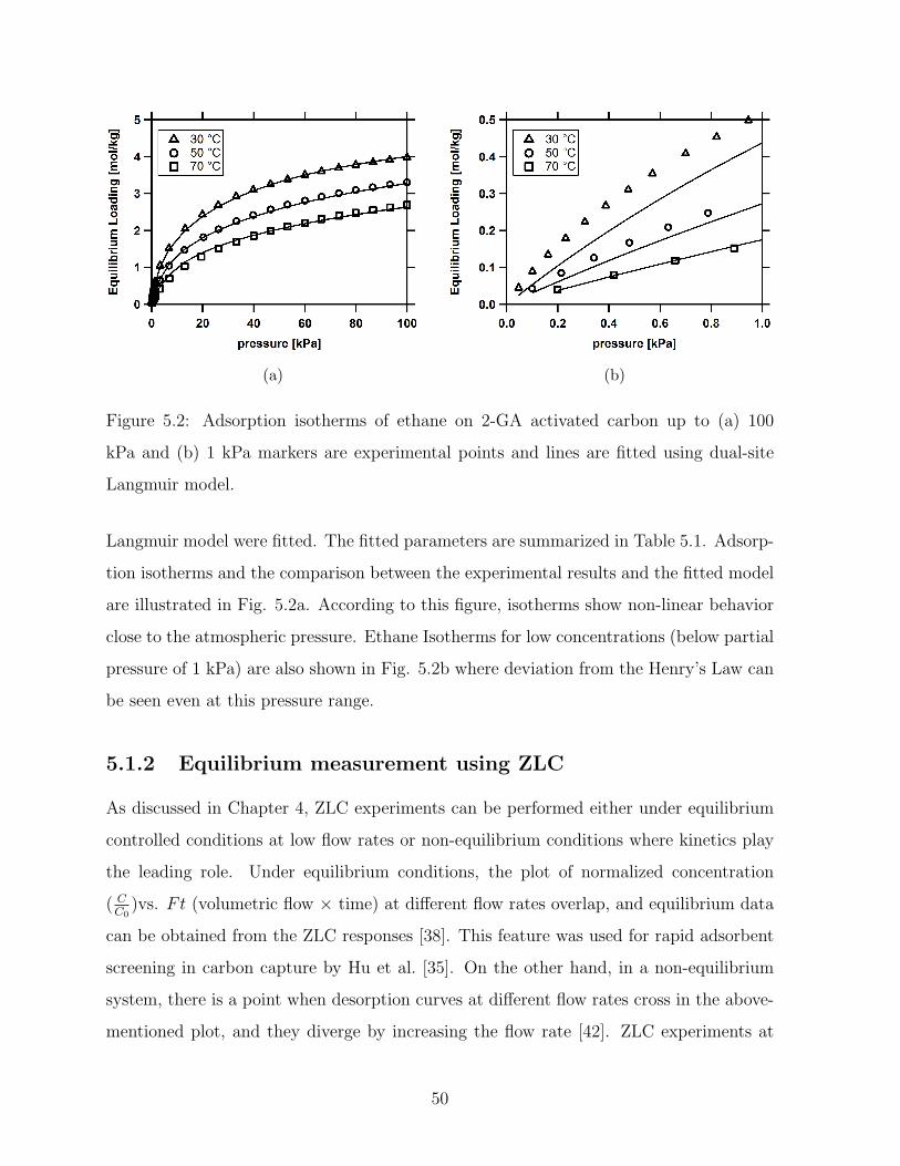
(a) (b)

Figure 5.2: Adsorption isotherms of ethane on 2-GA activated carbon up to (a) 100

kPa and (b) 1 kPa markers are experimental points and lines are fitted using dual-site

Langmuir model.

Langmuir model were fitted. The fitted parameters are summarized in Table 5.1. Adsorp-

tion isotherms and the comparison between the experimental results and the fitted model

are illustrated in Fig. 5.2a. According to this figure, isotherms show non-linear behavior

close to the atmospheric pressure. Ethane Isotherms for low concentrations (below partial

pressure of 1 kPa) are also shown in Fig. 5.2b where deviation from the Henry’s Law can

be seen even at this pressure range.

5.1.2 Equilibrium measurement using ZLC

As discussed in Chapter 4, ZLC experiments can be performed either under equilibrium

controlled conditions at low flow rates or non-equilibrium conditions where kinetics play

the leading role. Under equilibrium conditions, the plot of normalized concentration

( CC0

)vs. Ft (volumetric flow × time) at different flow rates overlap, and equilibrium data

can be obtained from the ZLC responses [38]. This feature was used for rapid adsorbent

screening in carbon capture by Hu et al. [35]. On the other hand, in a non-equilibrium

system, there is a point when desorption curves at different flow rates cross in the above-

mentioned plot, and they diverge by increasing the flow rate [42]. ZLC experiments at

50

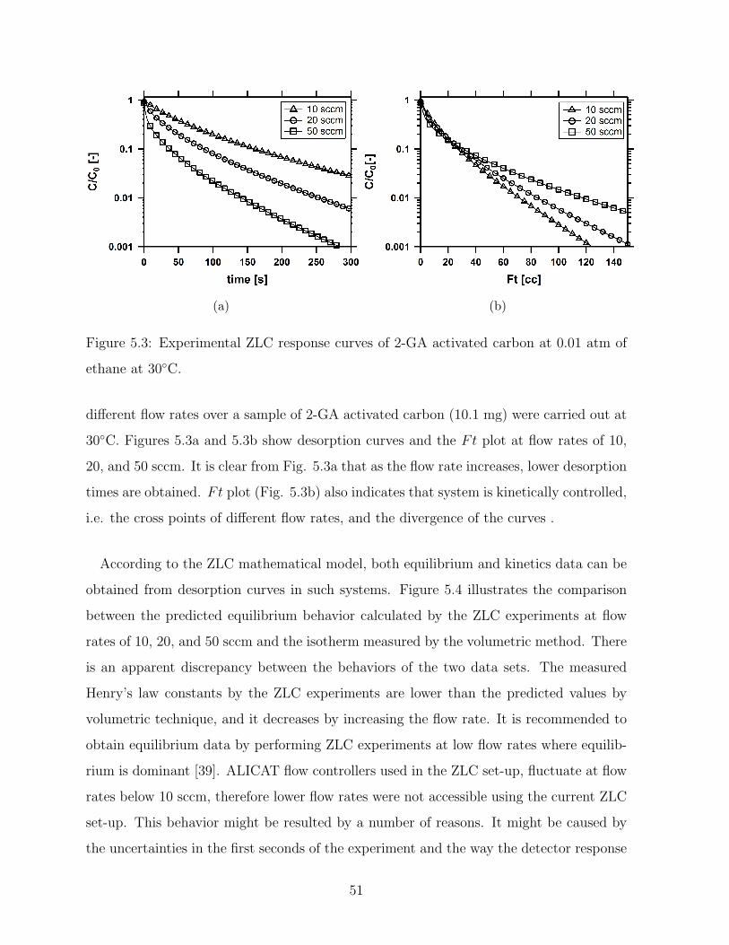
(a) (b)

Figure 5.3: Experimental ZLC response curves of 2-GA activated carbon at 0.01 atm of

ethane at 30C.

different flow rates over a sample of 2-GA activated carbon (10.1 mg) were carried out at

30C. Figures 5.3a and 5.3b show desorption curves and the Ft plot at flow rates of 10,

20, and 50 sccm. It is clear from Fig. 5.3a that as the flow rate increases, lower desorption

times are obtained. Ft plot (Fig. 5.3b) also indicates that system is kinetically controlled,

i.e. the cross points of different flow rates, and the divergence of the curves .

According to the ZLC mathematical model, both equilibrium and kinetics data can be

obtained from desorption curves in such systems. Figure 5.4 illustrates the comparison

between the predicted equilibrium behavior calculated by the ZLC experiments at flow

rates of 10, 20, and 50 sccm and the isotherm measured by the volumetric method. There

is an apparent discrepancy between the behaviors of the two data sets. The measured

Henry’s law constants by the ZLC experiments are lower than the predicted values by

volumetric technique, and it decreases by increasing the flow rate. It is recommended to

obtain equilibrium data by performing ZLC experiments at low flow rates where equilib-

rium is dominant [39]. ALICAT flow controllers used in the ZLC set-up, fluctuate at flow

rates below 10 sccm, therefore lower flow rates were not accessible using the current ZLC

set-up. This behavior might be resulted by a number of reasons. It might be caused by

the uncertainties in the first seconds of the experiment and the way the detector response

51

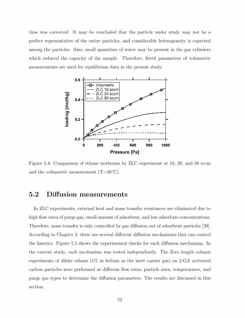
time was corrected. It may be concluded that the particle under study may not be a

perfect representative of the entire particles, and considerable heterogeneity is expected

among the particles. Also, small quantities of water may be present in the gas cylinders

which reduced the capacity of the sample. Therefore, fitted parameters of volumetric

measurements are used for equilibrium data in the present study.

Figure 5.4: Comparison of ethane isotherms by ZLC experiment at 10, 20, and 50 sccm

and the volumetric measurement (T=30C).

5.2 Diffusion measurements

In ZLC experiments, external heat and mass transfer resistances are eliminated due to

high flow rates of purge gas, small amount of adsorbent, and low adsorbate concentrations.

Therefore, mass transfer is only controlled by gas diffusion out of adsorbent particles [39].

According to Chapter 2, there are several different diffusion mechanisms that can control

the kinetics. Figure 5.5 shows the experimental checks for each diffusion mechanism. In

the current study, each mechanism was tested independently. The Zero length column

experiments of dilute ethane (1% in helium as the inert carrier gas) on 2-GA activated

carbon particles were performed at different flow rates, particle sizes, temperatures, and

purge gas types to determine the diffusion parameters. The results are discussed in this

section.

52

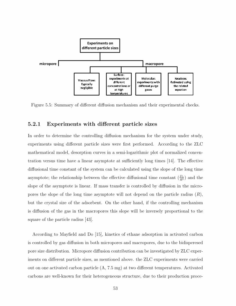
Figure 5.5: Summary of different diffusion mechanism and their experimental checks.

5.2.1 Experiments with different particle sizes

In order to determine the controlling diffusion mechanism for the system under study,

experiments using different particle sizes were first performed. According to the ZLC

mathematical model, desorption curves in a semi-logarithmic plot of normalized concen-

tration versus time have a linear asymptote at sufficiently long times [14]. The effective

diffusional time constant of the system can be calculated using the slope of the long time

asymptote; the relationship between the effective diffusional time constant (De

R2 ) and the

slope of the asymptote is linear. If mass transfer is controlled by diffusion in the micro-

pores the slope of the long time asymptote will not depend on the particle radius (R),

but the crystal size of the adsorbent. On the other hand, if the controlling mechanism

is diffusion of the gas in the macropores this slope will be inversely proportional to the

square of the particle radius [43].

According to Mayfield and Do [15], kinetics of ethane adsorption in activated carbon

is controlled by gas diffusion in both micropores and macropores, due to the bidisperesed

pore size distribution. Micropore diffusion contribution can be investigated by ZLC exper-

iments on different particle sizes, as mentioned above. the ZLC experiments were carried

out on one activated carbon particle (A, 7.5 mg) at two different temperatures. Activated

carbons are well-known for their heterogeneous structure, due to their production proce-

53

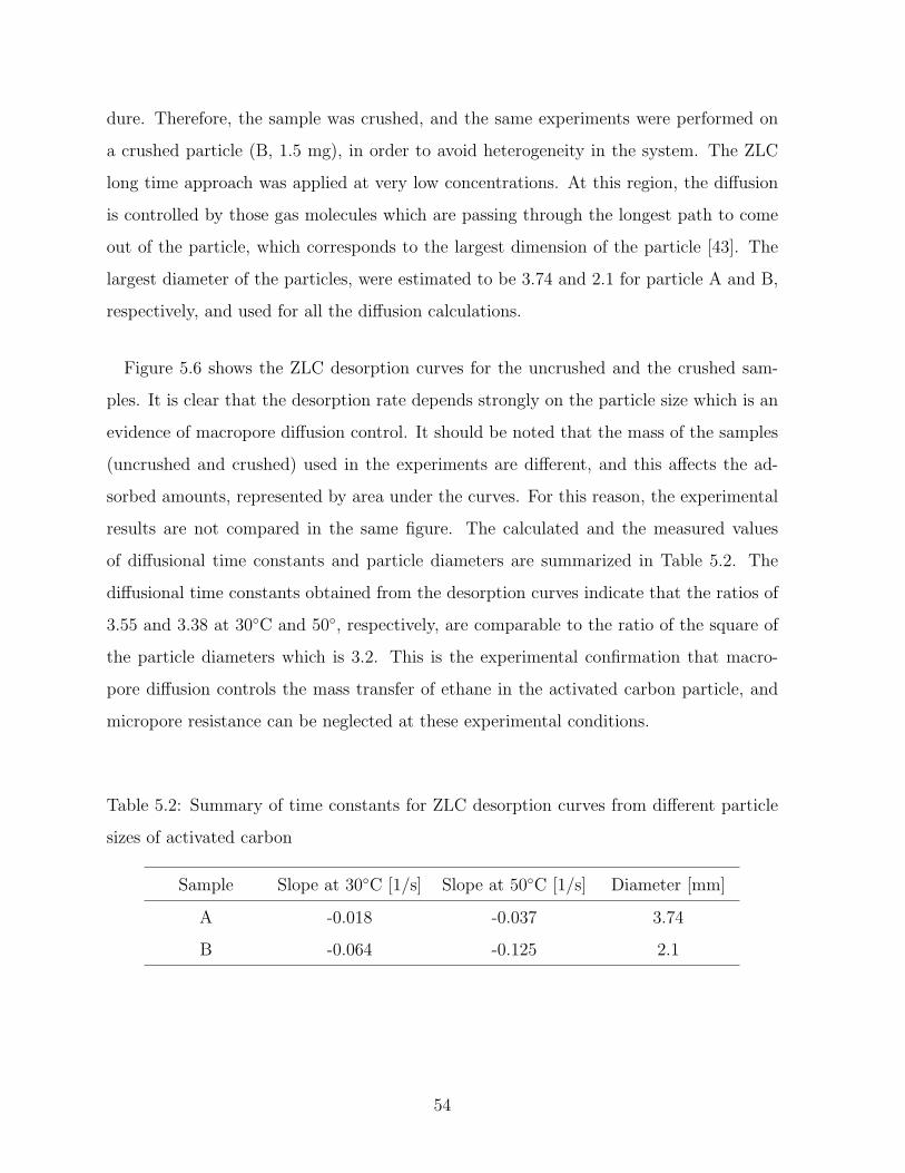
dure. Therefore, the sample was crushed, and the same experiments were performed on

a crushed particle (B, 1.5 mg), in order to avoid heterogeneity in the system. The ZLC

long time approach was applied at very low concentrations. At this region, the diffusion

is controlled by those gas molecules which are passing through the longest path to come

out of the particle, which corresponds to the largest dimension of the particle [43]. The

largest diameter of the particles, were estimated to be 3.74 and 2.1 for particle A and B,

respectively, and used for all the diffusion calculations.

Figure 5.6 shows the ZLC desorption curves for the uncrushed and the crushed sam-

ples. It is clear that the desorption rate depends strongly on the particle size which is an

evidence of macropore diffusion control. It should be noted that the mass of the samples

(uncrushed and crushed) used in the experiments are different, and this affects the ad-

sorbed amounts, represented by area under the curves. For this reason, the experimental

results are not compared in the same figure. The calculated and the measured values

of diffusional time constants and particle diameters are summarized in Table 5.2. The

diffusional time constants obtained from the desorption curves indicate that the ratios of

3.55 and 3.38 at 30C and 50, respectively, are comparable to the ratio of the square of

the particle diameters which is 3.2. This is the experimental confirmation that macro-

pore diffusion controls the mass transfer of ethane in the activated carbon particle, and

micropore resistance can be neglected at these experimental conditions.

Table 5.2: Summary of time constants for ZLC desorption curves from different particle

sizes of activated carbon

Sample Slope at 30C [1/s] Slope at 50C [1/s] Diameter [mm]

A -0.018 -0.037 3.74

B -0.064 -0.125 2.1

54

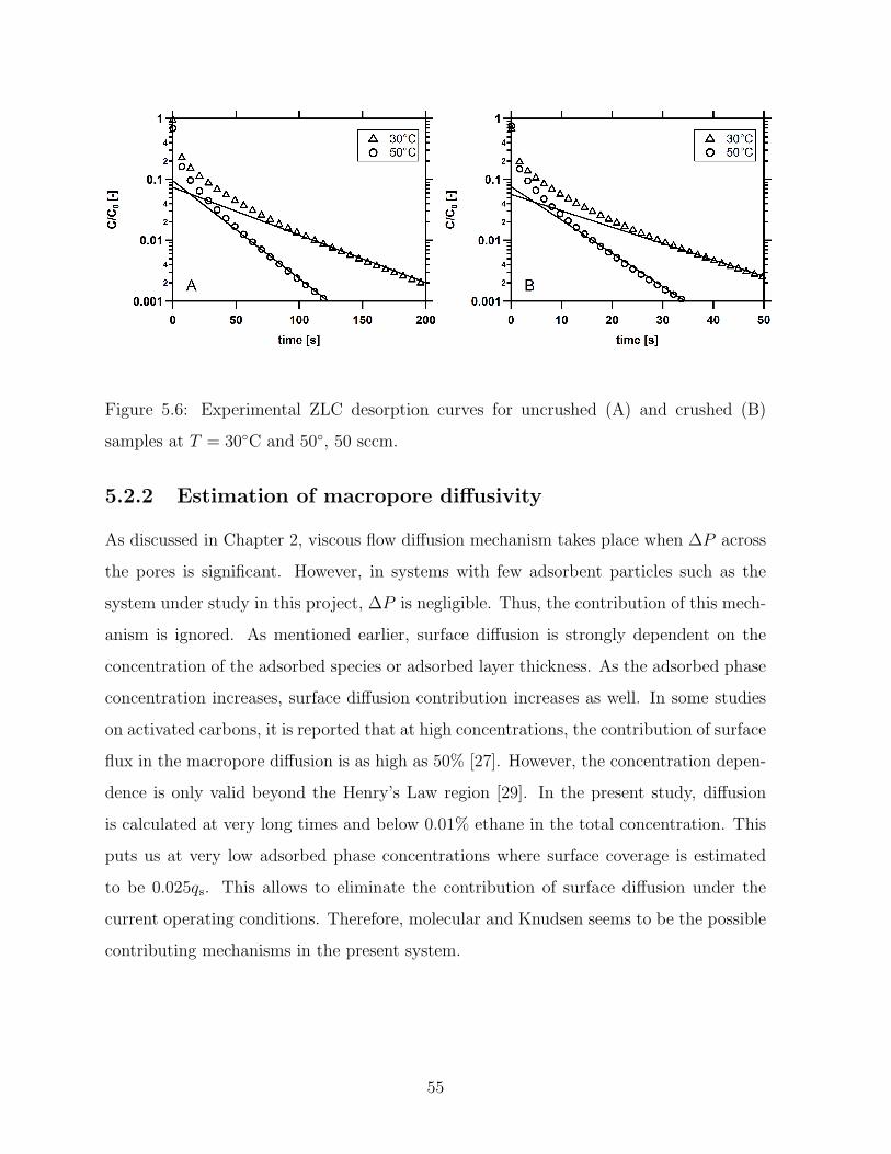
Figure 5.6: Experimental ZLC desorption curves for uncrushed (A) and crushed (B)

samples at T = 30C and 50, 50 sccm.

5.2.2 Estimation of macropore diffusivity

As discussed in Chapter 2, viscous flow diffusion mechanism takes place when ∆P across

the pores is significant. However, in systems with few adsorbent particles such as the

system under study in this project, ∆P is negligible. Thus, the contribution of this mech-

anism is ignored. As mentioned earlier, surface diffusion is strongly dependent on the

concentration of the adsorbed species or adsorbed layer thickness. As the adsorbed phase

concentration increases, surface diffusion contribution increases as well. In some studies

on activated carbons, it is reported that at high concentrations, the contribution of surface

flux in the macropore diffusion is as high as 50% [27]. However, the concentration depen-

dence is only valid beyond the Henry’s Law region [29]. In the present study, diffusion

is calculated at very long times and below 0.01% ethane in the total concentration. This

puts us at very low adsorbed phase concentrations where surface coverage is estimated

to be 0.025qs. This allows to eliminate the contribution of surface diffusion under the

current operating conditions. Therefore, molecular and Knudsen seems to be the possible

contributing mechanisms in the present system.

55

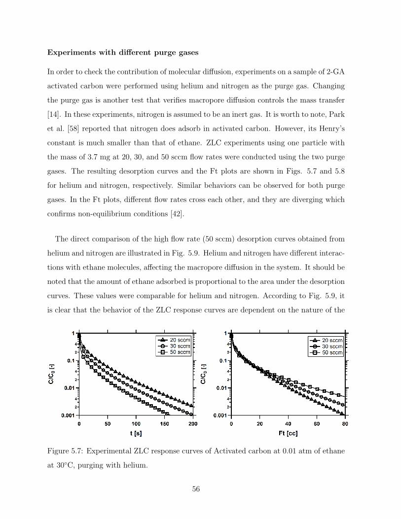
Experiments with different purge gases

In order to check the contribution of molecular diffusion, experiments on a sample of 2-GA

activated carbon were performed using helium and nitrogen as the purge gas. Changing

the purge gas is another test that verifies macropore diffusion controls the mass transfer

[14]. In these experiments, nitrogen is assumed to be an inert gas. It is worth to note, Park

et al. [58] reported that nitrogen does adsorb in activated carbon. However, its Henry’s

constant is much smaller than that of ethane. ZLC experiments using one particle with

the mass of 3.7 mg at 20, 30, and 50 sccm flow rates were conducted using the two purge

gases. The resulting desorption curves and the Ft plots are shown in Figs. 5.7 and 5.8

for helium and nitrogen, respectively. Similar behaviors can be observed for both purge

gases. In the Ft plots, different flow rates cross each other, and they are diverging which

confirms non-equilibrium conditions [42].

The direct comparison of the high flow rate (50 sccm) desorption curves obtained from

helium and nitrogen are illustrated in Fig. 5.9. Helium and nitrogen have different interac-

tions with ethane molecules, affecting the macropore diffusion in the system. It should be

noted that the amount of ethane adsorbed is proportional to the area under the desorption

curves. These values were comparable for helium and nitrogen. According to Fig. 5.9, it

is clear that the behavior of the ZLC response curves are dependent on the nature of the

Figure 5.7: Experimental ZLC response curves of Activated carbon at 0.01 atm of ethane

at 30C, purging with helium.

56

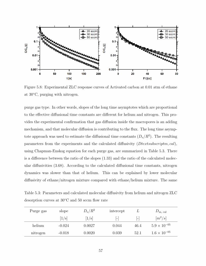
Figure 5.8: Experimental ZLC response curves of Activated carbon at 0.01 atm of ethane

at 30C, purging with nitrogen.

purge gas type. In other words, slopes of the long time asymptotes which are proportional

to the effective diffusional time constants are different for helium and nitrogen. This pro-

vides the experimental confirmation that gas diffusion inside the macropores is an adding

mechanism, and that molecular diffusion is contributing to the flux. The long time asymp-

tote approach was used to estimate the diffusional time constants (De/R2). The resulting

parameters from the experiments and the calculated diffusivity (Dtextsubscriptm, cal),

using Chapman-Enskog equation for each purge gas, are summarized in Table 5.3. There

is a difference between the ratio of the slopes (1.33) and the ratio of the calculated molec-

ular diffusivities (3.68). According to the calculated diffusional time constants, nitrogen

dynamics was slower than that of helium. This can be explained by lower molecular

diffusivity of ethane/nitrogen mixture compared with ethane/helium mixture. The same

Table 5.3: Parameters and calculated molecular diffusivity from helium and nitrogen ZLC

desorption curves at 30C and 50 sccm flow rate

Purge gas slope De/R2 intercept L Dm, cal

[1/s] [1/s] [-] [-] [m2/s]

helium -0.024 0.0027 0.044 46.4 5.9 × 10−05

nitrogen -0.018 0.0020 0.039 52.1 1.6 × 10−05

57

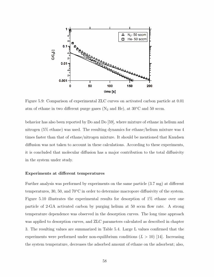
Figure 5.9: Comparison of experimental ZLC curves on activated carbon particle at 0.01

atm of ethane in two different purge gases (N2 and He), at 30C and 50 sccm.

behavior has also been reported by Do and Do [59], where mixture of ethane in helium and

nitrogen (5% ethane) was used. The resulting dynamics for ethane/helium mixture was 4

times faster than that of ethane/nitrogen mixture. It should be mentioned that Knudsen

diffusion was not taken to account in these calculations. According to these experiments,

it is concluded that molecular diffusion has a major contribution to the total diffusivity

in the system under study.

Experiments at different temperatures

Further analysis was performed by experiments on the same particle (3.7 mg) at different

temperatures, 30, 50, and 70C in order to determine macropore diffusivity of the system.

Figure 5.10 illustrates the experimental results for desorption of 1% ethane over one

particle of 2-GA activated carbon by purging helium at 50 sccm flow rate. A strong

temperature dependence was observed in the desorption curves. The long time approach

was applied to desorption curves, and ZLC parameters calculated as described in chapter

3. The resulting values are summarized in Table 5.4. Large L values confirmed that the

experiments were performed under non-equilibrium conditions (L > 10) [14]. Increasing

the system temperature, decreases the adsorbed amount of ethane on the adsorbent; also,

58

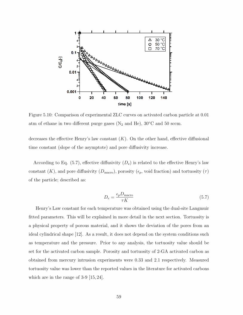
Figure 5.10: Comparison of experimental ZLC curves on activated carbon particle at 0.01

atm of ethane in two different purge gases (N2 and He), 30C and 50 sccm.

decreases the effective Henry’s law constant (K). On the other hand, effective diffusional

time constant (slope of the asymptote) and pore diffusivity increase.

According to Eq. (5.7), effective diffusivity (De) is related to the effective Henry’s law

constant (K), and pore diffusivity (Dmacro), porosity (εp, void fraction) and tortuosity (τ)

of the particle; described as:

De =εpDmacro

τK(5.7)

Henry’s Law constant for each temperature was obtained using the dual-site Langmuir

fitted parameters. This will be explained in more detail in the next section. Tortuosity is

a physical property of porous material, and it shows the deviation of the pores from an

ideal cylindrical shape [12]. As a result, it does not depend on the system conditions such

as temperature and the pressure. Prior to any analysis, the tortuosity value should be

set for the activated carbon sample. Porosity and tortuosity of 2-GA activated carbon as

obtained from mercury intrusion experiments were 0.33 and 2.1 respectively. Measured

tortuosity value was lower than the reported values in the literature for activated carbons

which are in the range of 3-9 [15,24].

59

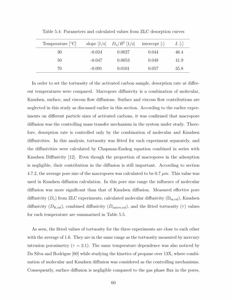
Table 5.4: Parameters and calculated values from ZLC desorption curves

Temperature [C] slope [1/s] De/R2 [1/s] intercept [-] L [-]

30 -0.024 0.0027 0.044 46.4

50 -0.047 0.0053 0.049 41.9

70 -0.091 0.0101 0.057 35.8

In order to set the tortuosity of the activated carbon sample, desorption rate at differ-

ent temperatures were compared. Macropore diffusivity is a combination of molecular,

Knudsen, surface, and viscous flow diffusions. Surface and viscous flow contributions are

neglected in this study as discussed earlier in this section. According to the earlier exper-

iments on different particle sizes of activated carbons, it was confirmed that macropore

diffusion was the controlling mass transfer mechanism in the system under study. There-

fore, desorption rate is controlled only by the combination of molecular and Knudsen

diffusivities. In this analysis, tortuosity was fitted for each experiment separately, and

the diffusivities were calculated by Chapman-Enskog equation combined in series with

Knudsen Diffusivity [12]. Even though the proportion of macropores in the adsorption

is negligible, their contribution in the diffusion is still important. According to section

4.7.2, the average pore size of the macropores was calculated to be 0.7 µm. This value was

used in Knudsen diffusion calculation. In this pore size range the influence of molecular

diffusion was more significant than that of Knudsen diffusion. Measured effective pore

diffusivity (De) from ZLC experiments, calculated molecular diffusivity (Dm,cal), Knudsen

diffusivity (DK,cal), combined diffusivity (Dmacro,cal), and the fitted tortuosity (τ) values

for each temperature are summarized in Table 5.5.

As seen, the fitted values of tortuosity for the three experiments are close to each other

with the average of 1.6. They are in the same range as the tortuosity measured by mercury

intrusion porosimetry (τ = 2.1). The same temperature dependence was also noticed by

Da Silva and Rodrigue [60] while studying the kinetics of propane over 13X, where combi-

nation of molecular and Knudsen diffusion was considered as the controlling mechanisms.

Consequently, surface diffusion is negligible compared to the gas phase flux in the pores,

60

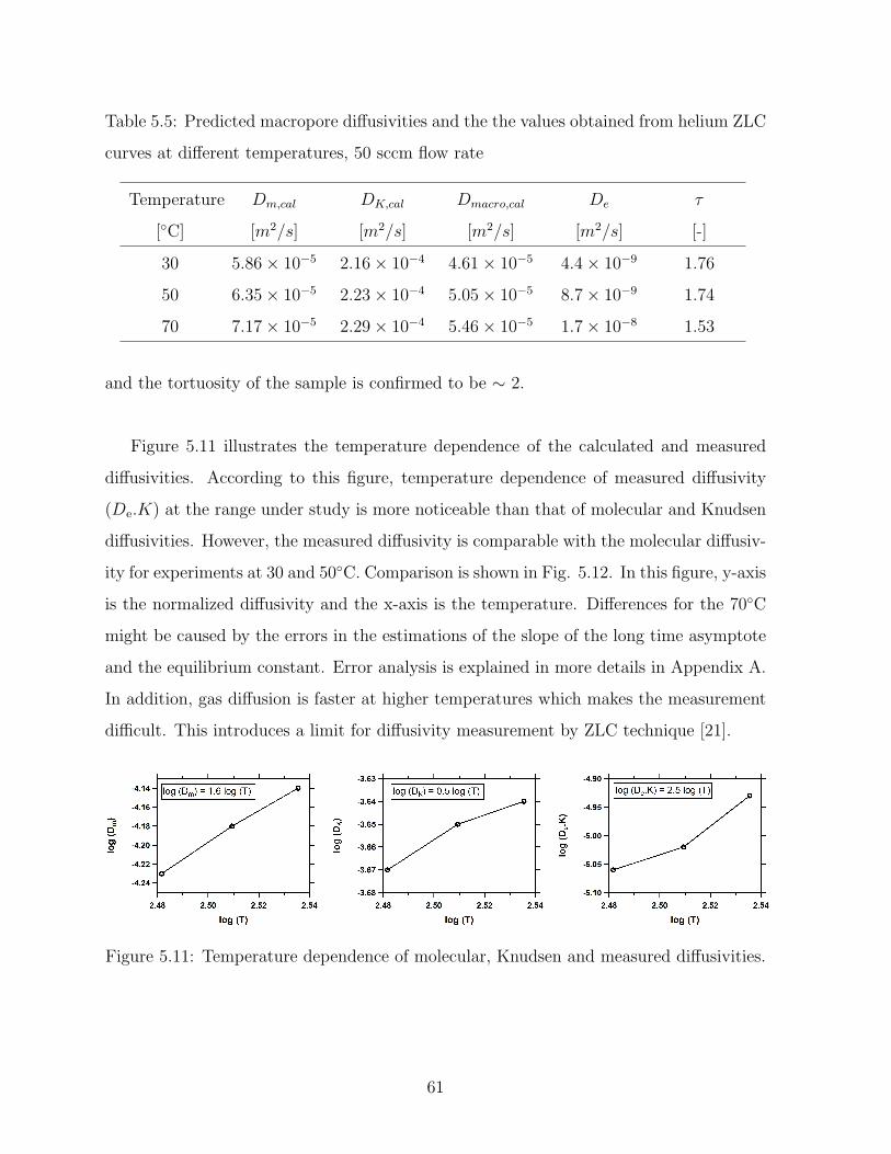
Table 5.5: Predicted macropore diffusivities and the the values obtained from helium ZLC

curves at different temperatures, 50 sccm flow rate

Temperature Dm,cal DK,cal Dmacro,cal De τ

[C] [m2/s] [m2/s] [m2/s] [m2/s] [-]

30 5.86 × 10−5 2.16 × 10−4 4.61 × 10−5 4.4 × 10−9 1.76

50 6.35 × 10−5 2.23 × 10−4 5.05 × 10−5 8.7 × 10−9 1.74

70 7.17 × 10−5 2.29 × 10−4 5.46 × 10−5 1.7 × 10−8 1.53

and the tortuosity of the sample is confirmed to be ∼ 2.

Figure 5.11 illustrates the temperature dependence of the calculated and measured

diffusivities. According to this figure, temperature dependence of measured diffusivity

(De.K) at the range under study is more noticeable than that of molecular and Knudsen

diffusivities. However, the measured diffusivity is comparable with the molecular diffusiv-

ity for experiments at 30 and 50C. Comparison is shown in Fig. 5.12. In this figure, y-axis

is the normalized diffusivity and the x-axis is the temperature. Differences for the 70C

might be caused by the errors in the estimations of the slope of the long time asymptote

and the equilibrium constant. Error analysis is explained in more details in Appendix A.

In addition, gas diffusion is faster at higher temperatures which makes the measurement

difficult. This introduces a limit for diffusivity measurement by ZLC technique [21].

Figure 5.11: Temperature dependence of molecular, Knudsen and measured diffusivities.

61

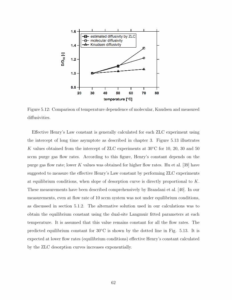
Figure 5.12: Comparison of temperature dependence of molecular, Knudsen and measured

diffusivities.

Effective Henry’s Law constant is generally calculated for each ZLC experiment using

the intercept of long time asymptote as described in chapter 3. Figure 5.13 illustrates

K values obtained from the intercept of ZLC experiments at 30C for 10, 20, 30 and 50

sccm purge gas flow rates. According to this figure, Henry’s constant depends on the

purge gas flow rate; lower K values was obtained for higher flow rates. Hu et al. [39] have

suggested to measure the effective Henry’s Law constant by performing ZLC experiments

at equilibrium conditions, when slope of desorption curve is directly proportional to K.

These measurements have been described comprehensively by Brandani et al. [40]. In our

measurements, even at flow rate of 10 sccm system was not under equilibrium conditions,

as discussed in section 5.1.2. The alternative solution used in our calculations was to

obtain the equilibrium constant using the dual-site Langmuir fitted parameters at each

temperature. It is assumed that this value remains constant for all the flow rates. The

predicted equilibrium constant for 30C is shown by the dotted line in Fig. 5.13. It is

expected at lower flow rates (equilibrium conditions) effective Henry’s constant calculated

by the ZLC desorption curves increases exponentially.

62

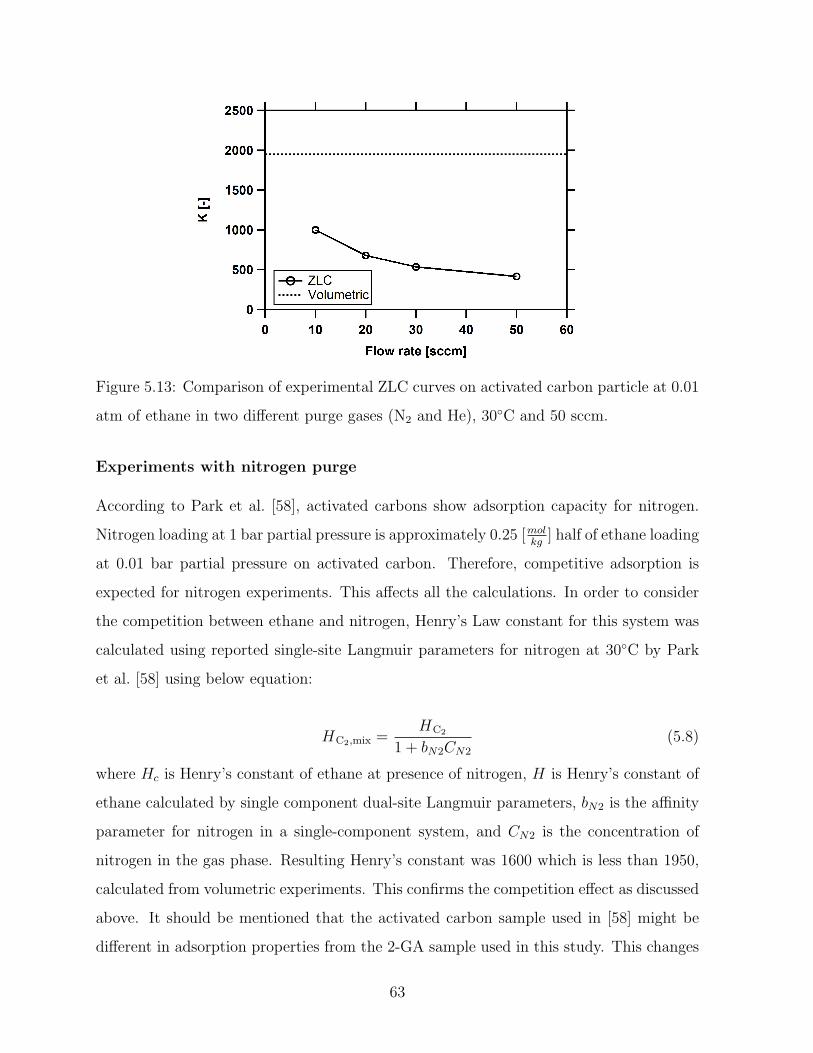
Figure 5.13: Comparison of experimental ZLC curves on activated carbon particle at 0.01

atm of ethane in two different purge gases (N2 and He), 30C and 50 sccm.

Experiments with nitrogen purge

According to Park et al. [58], activated carbons show adsorption capacity for nitrogen.

Nitrogen loading at 1 bar partial pressure is approximately 0.25 [molkg

] half of ethane loading

at 0.01 bar partial pressure on activated carbon. Therefore, competitive adsorption is

expected for nitrogen experiments. This affects all the calculations. In order to consider

the competition between ethane and nitrogen, Henry’s Law constant for this system was

calculated using reported single-site Langmuir parameters for nitrogen at 30C by Park

et al. [58] using below equation:

HC2,mix =HC2

1 + bN2CN2

(5.8)

where Hc is Henry’s constant of ethane at presence of nitrogen, H is Henry’s constant of

ethane calculated by single component dual-site Langmuir parameters, bN2 is the affinity

parameter for nitrogen in a single-component system, and CN2 is the concentration of

nitrogen in the gas phase. Resulting Henry’s constant was 1600 which is less than 1950,

calculated from volumetric experiments. This confirms the competition effect as discussed

above. It should be mentioned that the activated carbon sample used in [58] might be

different in adsorption properties from the 2-GA sample used in this study. This changes

63

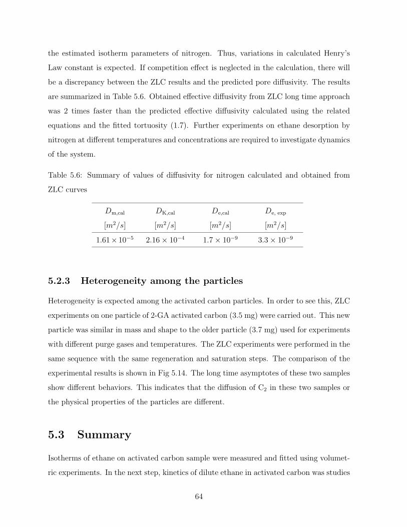
the estimated isotherm parameters of nitrogen. Thus, variations in calculated Henry’s

Law constant is expected. If competition effect is neglected in the calculation, there will

be a discrepancy between the ZLC results and the predicted pore diffusivity. The results

are summarized in Table 5.6. Obtained effective diffusivity from ZLC long time approach

was 2 times faster than the predicted effective diffusivity calculated using the related

equations and the fitted tortuosity (1.7). Further experiments on ethane desorption by

nitrogen at different temperatures and concentrations are required to investigate dynamics

of the system.

Table 5.6: Summary of values of diffusivity for nitrogen calculated and obtained from

ZLC curves

Dm,cal DK,cal De,cal De, exp

[m2/s] [m2/s] [m2/s] [m2/s]

1.61× 10−5 2.16 × 10−4 1.7 × 10−9 3.3 × 10−9

5.2.3 Heterogeneity among the particles

Heterogeneity is expected among the activated carbon particles. In order to see this, ZLC

experiments on one particle of 2-GA activated carbon (3.5 mg) were carried out. This new

particle was similar in mass and shape to the older particle (3.7 mg) used for experiments

with different purge gases and temperatures. The ZLC experiments were performed in the

same sequence with the same regeneration and saturation steps. The comparison of the

experimental results is shown in Fig 5.14. The long time asymptotes of these two samples

show different behaviors. This indicates that the diffusion of C2 in these two samples or

the physical properties of the particles are different.

5.3 Summary

Isotherms of ethane on activated carbon sample were measured and fitted using volumet-

ric experiments. In the next step, kinetics of dilute ethane in activated carbon was studies

64

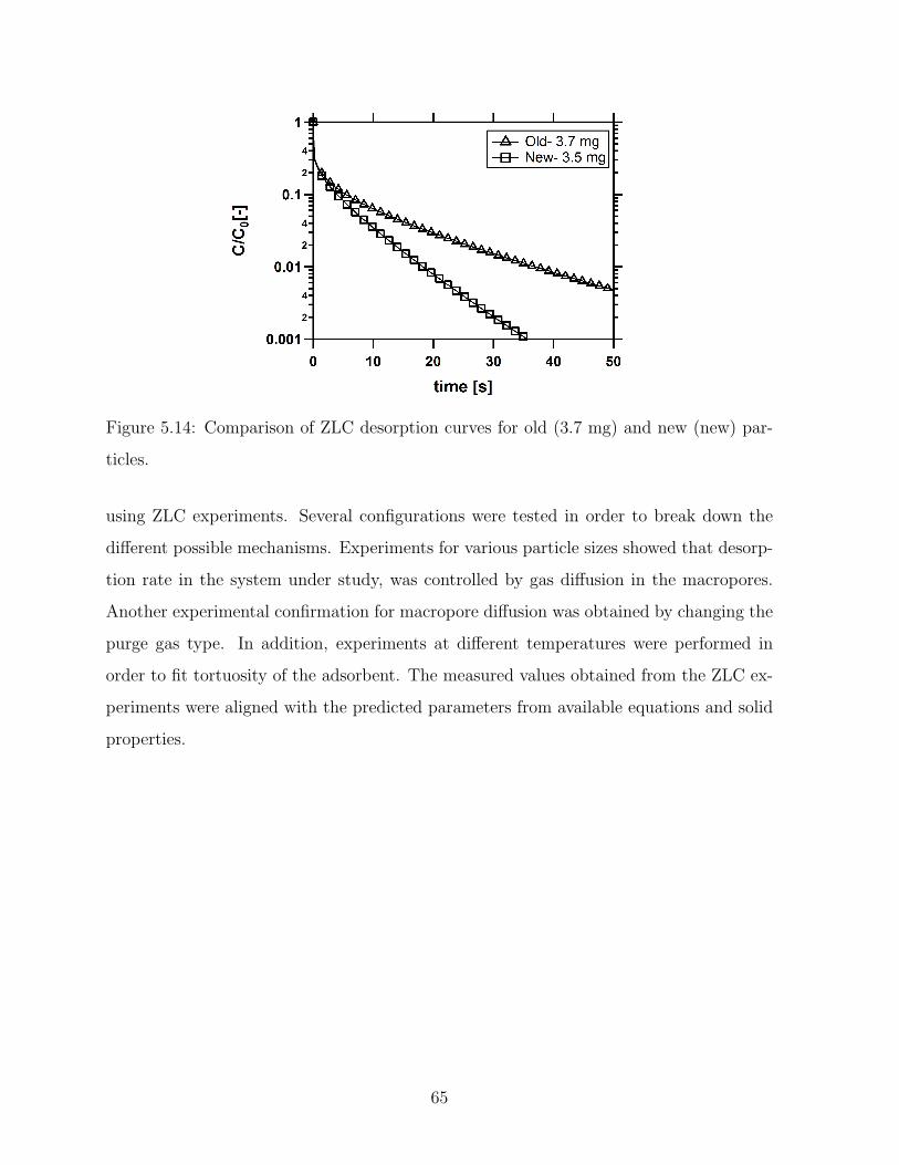
Figure 5.14: Comparison of ZLC desorption curves for old (3.7 mg) and new (new) par-

ticles.

using ZLC experiments. Several configurations were tested in order to break down the

different possible mechanisms. Experiments for various particle sizes showed that desorp-

tion rate in the system under study, was controlled by gas diffusion in the macropores.

Another experimental confirmation for macropore diffusion was obtained by changing the

purge gas type. In addition, experiments at different temperatures were performed in

order to fit tortuosity of the adsorbent. The measured values obtained from the ZLC ex-

periments were aligned with the predicted parameters from available equations and solid

properties.

65

Chapter 6

Conclusions and Recommendations

This study was focused on determination of diffusion in porous materials using the ZLC

method. The main advantages and limitations of this approach have been noted in chap-

ters 3 and 5. This information is summarized in this chapter.

In the present work, diffusion measurements of dilute ethane on 2-GA activated carbon

particles manufactured by Kuraray Co. were completed. Solid characterization measure-

ments were performed using mercury intrusion porosimetry and N2 adsorption techniques

prior to the ZLC experiments. Physical properties of the adsorbent sample were analyzed.

Pore size distribution, porosity, and tortuosity of the sample were determined and com-

pared to the values reported in the literature. Isotherms of ethane on activated carbon at

different temperatures were measured using volumetric method, and the dual-site Lang-

muir parameters were fitted to the experimental data using non-linear regression. The

ZLC set-up was built during the course of this project. Flame ionization detector was

used as the sensitive detector connected to the outlet of the ZLC set-up, in order to mon-

itor the concentration of ethane in the effluent gas. Dead volume measurements resulted

the value of 0.5 cc, which is comparable to data published in the literature. ZLC method

depends on following the desorption curve measured at sufficiently high flow rates when

system is under non-equilibrium conditions, and desorption rate is controlled by diffusion.

66

The experiments provided useful methods for studying the diffusion mechanism of the

test gas in the adsorbent particles. Experimental results i.e. Ft plots indicated that

under the studied conditions, desorption rate was controlled by diffusion of gas out of

adsorbent particles. Different particle sizes of the activated carbon were tested, in order

to verify the diffusion mechanism. The experimental results were affected by the particle

sizes. This confirms macropore diffusion in the system under study. Surface diffusion was

neglected in this study because the ZLC experiments were performed at very low surface

coverage. Also, viscous flow diffusion was overpassed, due to insignificant pressure drop

across the adsorbent particle. According to the experiments on different purge gas types,

it was observed that the desorption rates were dependent on the nature of the purge

gas. Diffusional time constants for nitrogen were slower than helium. This is related to

different interactions that are between molecules in ethane/helium and ethane/nitrogen

mixtures. Therefore, macropore diffusion was assumed to be the contribution of molecular

and Knudsen diffusivities. There was a good agreement between the calculated diffusiv-

ities from equations, solid properties obtained from characterization tests and the ZLC

experiments.

6.1 Recommendations

ZLC measurements were carried out on one particle of the adsorbent. However, activated

carbons have shown heterogeneity within the sample batch. Therefore, it is recommended

to study adsorption/desorption characteristics in such systems on bulk amounts of the

sample. If the aim is to understand the diffusion mechanisms, ZLC technique will be a

suitable candidate, providing reliable estimation of the diffusivity values. Another limita-

tion in the present study was the equilibrium measurements. Due to the flow controllers

used in the current ZLC set-up, equilibrium conditions were not achievable to collect

isotherm data. It is recommended for the future works to study equilibrium measure-

ments on ZLC prior to diffusion experiments using suitable flow controllers. Furthermore,

in order to avoid trace amounts of water in the cylinders, it is suggested to add drying

columns downstream of the gas cylinders. This enhances the measured capacity of ad-

67

sorbent in ZLC experiments. In order to observe the contribution of surface diffusion

to the total desorption rate, ZLC experiments at higher concentrations of ethane can be

performed. This can be achieve by adding an ethane stream to the test line before the

main switching valve, in order to attain concentrated gas. It is recommended to perform

the experiments differentially to study the concentration dependence of surface diffusion

in the system under study.

The diffusivity value obtained from ZLC experiment for nitrogen purge, was not fully in

line with the predicted diffusivities using the related equations. It was approximately two

times faster than that of the combination of molecular and Knudsen for ethane/nitrogen

mixture. It may be caused by competition between nitrogen and ethane. It is suggested

to measure nitrogen isotherms of the activated carbon sample at different temperatures,

and perform ZLC experiments using nitrogen purge at those temperatures. Therefore,

the comparison between the experimental results and predicted diffusivities develops a

better understanding of the system. Experiments on dilute ethane in nitrogen carrier gas

and different purge gases will also provide good insight to the matter, and will show the

effect of carrier gas in the experiments.

68

Bibliography

[1] Q. Wang, X. Chen, A. N. Jha, and H. Rogers, “Natural Gas from Shale Formation

The Evolution, Evidences and Challenges of Shale Gas Revolution in United States,”

Renewable Sustainable Energy Rev., vol. 30, pp. 1–28, 2014.

[2] Internatinal Energy Agency, OECD/IEA 2016 Key Natural Gas Trends. IEA Pub-

lishing, 2016.

[3] The Alberta Energy Resources Conservation Board, Alberta’s Energy Industry an

Overview. Government of Alberta, 2012.

[4] Gas Processors Association Board of Authors, 11th Edition GPSA Engineering Data

Book. Gas Processors Suppliers Association, 1998.

[5] S. Thomas, “Enhanced Oil Recovery-an Overview,” Oil Gas Sci. Technol., vol. 63,

pp. 9–19, 2008.

[6] M. Huff and L. D. Schmidt, “Ethylene Formation by Oxidative Dehydrogenation

of Ethane Over Monoliths at Very Short Contact Times,” J. Phys. Chem., vol. 97,

pp. 11815–11822, 1993.

[7] M. Arruebo, J. Coronas, M. Menendez, and J. Santamarıa, “Separation of Hydrocar-

bons from Natural Gas Using Silicalite Membranes,” Sep. Purif. Technol., vol. 25,

pp. 275–286, 2001.

[8] N. Magnowski, A. Avila, C. Lin, M. Shi, and S. Kuznicki, “Extraction of Ethane

from Natural Gas by Adsorption on Modified ETS-10,” Chem. Eng. Sci., vol. 66,

pp. 1697–1701, 2011.

69

[9] L. E. Perez, A. M. Avila, J. A. Sawada, A. Rajendran, and S. M. Kuznicki, “Process

Optimization-Based Adsorbent Selection for Ethane Recovery from Residue Gas,”

Sep. Purif. Technol., vol. 168, pp. 19–31, 2016.

[10] A. Malek and S. Farooq, “Kinetics of Hydrocarbon Adsorption on Activated Carbon

and Silica Gel,” AIChE J., vol. 43, pp. 761–776, 1997.

[11] A. Malek and S. Farooq, “Determination of Equilibrium Isotherms Using Dynamic

Column Breakthrough and Constant Flow Equilibrium Desorption,” J. Chem. Eng.

Data, vol. 41, pp. 25–32, 1996.

[12] D. Ruthven, Principles of Adsorption and Adsorption Processes. Wiley, 1984.

[13] R. T. Yang, Gas Separation by Adsorption Processes. Butterworths, 1987.

[14] M. Eic and D. M. Ruthven, “A New Experimental Technique for Measurement of

Intracrystalline Diffusivity,” Zeolites, vol. 8, pp. 40–45, 1988.

[15] P. Mayfield and D. Do, “Measurement of the Single-Component Adsorption Kinetics

of Ethane, Butane and Pentane onto Activated Carbon Using a Differential Adsorp-

tion Bed,” Ind. Eng. Chem. Res., 1991.

[16] R. Bansal, Activated Carbon Adsorption. Taylor & Francis, 2005.

[17] M. Thommes, K. Kaneko, A. V. Neimark, J. P. Olivier, F. Rodriguez-Reinoso, J. Rou-

querol, and K. S. Sing, “Physisorption of Gases, with Special Reference to the Eval-

uation of Surface Area and Pore Size Distribution (IUPAC Technical Report),” Pure

Appl. Chem., vol. 87, pp. 1051–1069, 2015.

[18] H. Giesche, “Mercury Porosimetry: a General (Practical) Overview,” Part. Part.

Syst. Char., vol. 23, pp. 9–19, 2006.

[19] L. E. Perez, “Ethane Recovery from Residue Gas Using Pressure Swing Adsorption,”

Master’s thesis, University of Alberta, 2015.

70

[20] S. A. Hosseinzadeh Hejazi, A. Rajendran, J. A. Sawada, and S. M. Kuznicki, “Dy-

namic Column Breakthrough and Process Studies of High-Purity Oxygen Production

Using Silver Exchanged Titanosilicates (Ag-ETS-10),” Ind. Eng. Chem. Res., vol. 55,

p. 59936005, 2016.

[21] J. Karger, D. M. Ruthven, and D. N. Theodorou, Diffusion in Nanoporous Materials.

Wiley-VCH, 2012.

[22] R. Bird, W. Stewart, and E. Lightfoot, Transport Phenomena. J. Wiley, 2002.

[23] S. Sircar, T. Golden, and M. Rao, “Activated Carbon for Gas Separation and Stor-

age,” Carbon, vol. 34, pp. 1–12, 1996.

[24] P. Gray and D. Do, “Adsorption and Desorption of Gaseous Sorbates on a Bidis-

persed Particle with Freundlich Isotherm: II. Experimental Study of Sulphur Dioxide

Sorption on Activated Carbon Particles,” Gas Sep. Purif., vol. 3, pp. 201–208, 1989.

[25] I. Neretnieks, “Analysis of Some Adsorption Experiments with Activated Carbon,”

Chem. Eng. Sci., vol. 31, pp. 1029–1035, 1976.

[26] P. G. Gray and D. D. Do, “Dynamics of Carbon Dioxide Sorption on Activated-

Carbon Particles,” AIChE J., vol. 37, pp. 1027–1034, 1991.

[27] S.-J. Doong and R. Yang, “Bulk Separation of Multicomponent Gas Mixtures

by Pressure Swing Adsorption: Pore/Surface Diffusion and Equilibrium Models,”

AIChE J., vol. 32, pp. 397–410, 1986.

[28] D. Do, X. Hu, and P. Mayfield, “Multicomponent Adsorption of Ethane, n-butane

and n-pentane in activated carbon,” Gas Sep. Purif., vol. 5, pp. 35–48, 1991.

[29] A. Kapoor, R. T. Yang, and C. Wong, “Surface Diffusion,” Catalysis Reviews, vol. 31,

pp. 129–214, 1989.

[30] S. Bhatia and D. Do, “On the Concentration Dependence of Surface Diffusion Coeffi-

cients in Capillary Porous Materials,” in Proceedings of the Royal Society of London

A: Mathematical, Physical and Engineering Sciences, vol. 434, 1991.

71

[31] D. D. Do, “A Model for Surface dDiffusion of Ethane and propane in Activated

Carbon,” Chem. Eng. Sci., vol. 51, pp. 4145–4158, 1996.

[32] X. Hu, D. Do, and G. Rao, “Experimental Concentration Dependence of Surface Dif-

fusivity of Hydrocarbons in Activated Carbon,” Chem. Eng. Sci., vol. 49, pp. 2145–

2152, 1994.

[33] X. Hu and D. D. Do, “Multicomponent Adsorption Kinetics of Hydrocarbons onto

Activated Carbon: Contribution of Micropore Resistance,” Chem. Eng. Sci., vol. 48,

pp. 1317–1323, 1993.

[34] X. Hu, S. Brandani, A. I. Benin, and R. R. Willis, “Development of a Semiautomated

Zero Zength Column Technique for Carbon Capture Applications: Study of Diffusion

Behavior of CO2 in MOFs,” Ind. Eng. Chem. Res., vol. 54, pp. 5777–5783, 2015.

[35] X. Hu, S. Brandani, A. I. Benin, and R. R. Willis, “Development of a Semiautomated

Zero Length Column Technique for Carbon Capture Applications: Rapid Capacity

Ranking of Novel Adsorbents,” Ind. Eng. Chem. Res., vol. 54, pp. 6772–6780, 2015.

[36] J. A. Silva, F. A. Da Silva, and A. E. Rodrigues, “An Analytical Solution for the

Analysis of Zero-Length-Column Experiments with Heat Effects,” Ind. Eng. Chem.

Res., vol. 40, no. 16, pp. 3697–3702, 2001.

[37] W. Duncan and K. Moller, “A zero lengthcriterion for ZLC chromatography,” Chem.

Eng. Sci., vol. 55, no. 22, pp. 5415–5420, 2000.

[38] F. Brandani, Development and Application of the Zero Length Column (ZLC)

Techique for Measuring Adsorption Equilibria. PhD thesis, University of Maine,

2002.

[39] X. Hu, E. Mangano, D. Friedrich, H. Ahn, and S. Brandani, “Diffusion Mechanism

of CO2 in 13X Zeolite Beads,” Adsorption, vol. 20, pp. 121–135, 2014.

[40] F. Brandani, D. Ruthven, and C. G. Coe, “Measurement of Adsorption Equilibrium

by the Zero Length Column (ZLC) Technique Part 1: Single-Component Systems,”

Ind. Eng. Chem. Res., vol. 42, pp. 1451–1461, 2003.

72

[41] F. Brandani and D. Ruthven, “Measurement of Adsorption Equilibria by the Zero

Length Column (ZLC) Technique Part 2: Binary Systems,” Ind. Eng. Chem. Res.,

vol. 42, pp. 1462–1469, 2003.

[42] S. Brandani, “A Simple Graphical Check of Consistency for Zero Length Column

Desorption Curves,” Chem. Eng. Technol., vol. 39, pp. 1194–1198, 2016.

[43] D. M. Ruthven and Z. Xu, “Diffusion of Oxygen and Nitrogen in 5A Zeolite Crystals

and Commercial 5A Pellets,” Chem. Eng. Sci., vol. 48, pp. 3307–3312, 1993.

[44] A. Vidoni and D. M. Ruthven, “Diffusion of C2H6 and C2H4 in DDR Zeolite,” Ind.

Eng. Chem. Res., vol. 51, pp. 1383–1390, 2012.

[45] S. Brandani, J. Hufton, and D. Ruthven, “Self-Diffusion of Propane and Propylene in

5A and 13X zeolite Crystals Studied by the Tracer ZLC Method,” Zeolites, vol. 15,

pp. 624–631, 1995.

[46] D. M. Ruthven and P. Stapleton, “Measurement of Liquid Phase Counter-Diffusion

in Zeolite Crystals by the ZLC Method,” Chem. Eng. Sci., vol. 48, pp. 89–98, 1993.

[47] S. Brandani, “Effects of Nonlinear Equilibrium on Zero Length Column Experi-

ments,” Chem. Eng. Sci., vol. 53, pp. 2791–2798, 1998.

[48] S. Brandani, C. Cavalcante, A. Guimaraes, and D. Ruthven, “Heat Effects in ZLC

Experiments,” Adsorption, vol. 4, pp. 275–285, 1998.

[49] S. Brandani, “Analytical Solution for ZLC Desorption Curves with Bi-porous Adsor-

bent Particles,” Chem. Eng. Sci., vol. 51, pp. 3283–3288, 1996.

[50] S. Brandani and D. M. Ruthven, “Analysis of ZLC Desorption Curves for Liquid

Systems,” Chem. Eng. Sci., 1995.

[51] S. Brandani, M. A. Jama, and D. M. Ruthven, “Zlc Measurements under Non-linear

Conditions,” Chem. Eng. Sci., vol. 55, pp. 1205–1212, 2000.

73

[52] J. A. Silva, K. Schumann, and A. E. Rodrigues, “Sorption and Kinetics of CO2 and

CH4 in Binderless Beads of 13X Zeolite,” Microporous Mesoporous Mater., vol. 158,

pp. 219–228, 2012.

[53] O. Auban, J. Malet, P. Brun, J. Brinster, J. Quillico, and E. Studer, “Implementa-

tion of Gas Concentration Measurement Systems Using Mass Spectrometry inCon-

tainment Thermal-Hydraulics Test Facilities: Different Approaches for Calibration

and Measurement with Steam/Air/Helium Mixtures,” in 10th International Topical

Meeting on Nuclear Reactor Thermal Hydraulics (NURETH-10), Seoul, Korea, 2003.

[54] P. A. Webb, “An Introduction to the Physical Characterization of Materials by Mer-

cury Intrusion Porosimetry with Emphasis on Reduction and Presentation of Exper-

imental Data,” Micromeritics Instrument Corp, Norcross, Georgia, 2001.

[55] K. Sing, “The Use of Nitrogen Adsorption for the Characterisation of Porous Mate-

rials,” Colloids Surf., A, vol. 187, pp. 3–9, 2001.

[56] S. Brunauer, P. H. Emmett, and E. Teller, “Adsorption of Gases in Multimolecular

Layers,” J. Am. Chem. Soc., vol. 60, pp. 309–319, 1938.

[57] J. De Boer, B. Linsen, and T. J. Osinga, “Studies on Pore Systems in Catalysts: VI.

The Universal t Curve,” J. Catal., vol. 4, pp. 643–648, 1965.

[58] Y. Park, D.-K. Moon, Y.-H. Kim, H. Ahn, and C.-H. Lee, “Adsorption Isotherms

of CO2, CO, N2, CH4, Ar and H2 on Activated Carbon and Zeolite LiX up to 1.0

MPa,” Adsorption, vol. 20, pp. 631–647, 2014.

[59] H. Do and D. Do, “Maxwell-Stefan Analysis of Multicomponent Transient Diffusion

in a Capillary and Adsorption of Hydrocarbons in Activated Carbon Particle,” Chem.

Eng. Sci., vol. 53, pp. 1239–1252, 1998.

[60] F. A. Da Silva and A. E. Rodrigues, “Adsorption Equilibria and Kinetics for Propy-

lene and Propane over 13X and 4A Zeolite Pellets,” Ind. Eng. Chem. Res., vol. 38,

pp. 2051–2057, 1999.

74

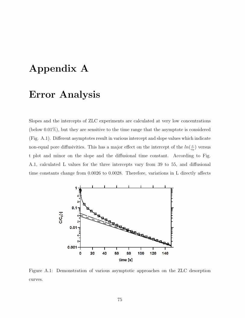
Appendix A

Error Analysis

Slopes and the intercepts of ZLC experiments are calculated at very low concentrations

(below 0.01%), but they are sensitive to the time range that the asymptote is considered

(Fig. A.1). Different asymptotes result in various intercept and slope values which indicate

non-equal pore diffusivities. This has a major effect on the intercept of the ln( cc0

) versus

t plot and minor on the slope and the diffusional time constant. According to Fig.

A.1, calculated L values for the three intercepts vary from 39 to 55, and diffusional

time constants change from 0.0026 to 0.0028. Therefore, variations in L directly affects

Figure A.1: Demonstration of various asymptotic approaches on the ZLC desorption

curves.

75

the calculated pore diffusivity. In order to eliminate this, Henry’s Law constants were

calculated using the fitted parameters for the volumetric equilibrium measurements. It is

worthwhile to remind that the measured loadings using ZLC experiments are lower than

those predicted from volumetric method. Uncertainty in the calculated pore diffusivity is

expected, as caused by the variations in the slope of the ZLC asymptote and the considered

equilibrium constant. The expected uncertainty is calculated according to Eq. A.1, where

∆De is the variations of the effective diffusivity and ∆K is the expected uncertainty in

effective Henry’s constant. Effective pore diffusivity variation is approximately 1 × 10−6.

This will change the fitted tortuosity in the range of 2.5 to 1.5.

∆Dmacro = ((∂Dmacro

∂De

∆De)2 + (

∂Dmacro

∂K∆K)2)0.5 (A.1)

76

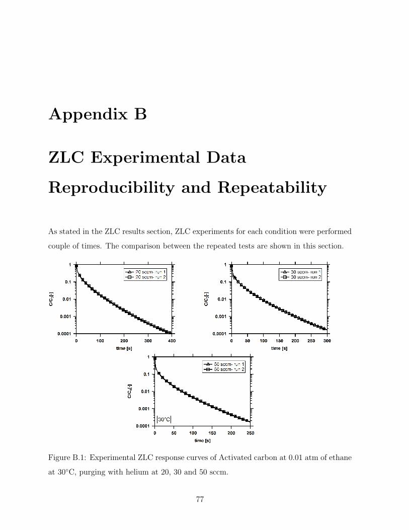
Appendix B

ZLC Experimental Data

Reproducibility and Repeatability

As stated in the ZLC results section, ZLC experiments for each condition were performed

couple of times. The comparison between the repeated tests are shown in this section.

Figure B.1: Experimental ZLC response curves of Activated carbon at 0.01 atm of ethane

at 30C, purging with helium at 20, 30 and 50 sccm.

77

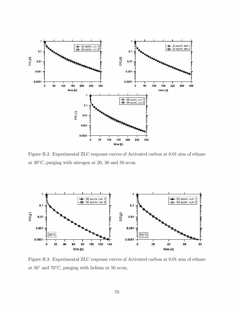
Figure B.2: Experimental ZLC response curves of Activated carbon at 0.01 atm of ethane

at 30C, purging with nitrogen at 20, 30 and 50 sccm.

Figure B.3: Experimental ZLC response curves of Activated carbon at 0.01 atm of ethane

at 50 and 70C, purging with helium at 50 sccm.

78