SYSTEM MODELLING AND TESTING OF A MAGNETIC …

SYSTEM MODELLING AND TESTING OF A MAGNETIC

SUSCEPTIBILITY DEVICE AND EFFECT OF DOWNHOLE

IN-SITU TEMPERATURES ON MAGNETIC SUSCEPTIBILITY

Arfan Ali

Submitted for the

Degree of Doctor of Philosophy in

Petroleum Engineering

Heriot-Watt University

Institute of Petroleum Engineering

Edinburgh

United Kingdom

April 2009

This copy of the thesis has been supplied on conditions that anyone who consults it is

understood to recognize that the copyright rests with its author and that no quotation from the

thesis and no information derived from it may be published without the prior written consent of

the author or of the University (as may be appropriate)

ACADEMIC REGISTRY Research Thesis Submission

Name Arfan Ali

SchoolPGI Institute of Petroleum Engineering (IPE)

Version (ie First Resubmission Final)

Final Degree Sought (Award and Subject area)

PhD

Declaration In accordance with the appropriate regulations I hereby submit my thesis and I declare that 1) the thesis embodies the results of my own work and has been composed by myself 2) where appropriate I have made acknowledgement of the work of others and have made reference to

work carried out in collaboration with other persons 3) the thesis is the correct version of the thesis for submission and is the same version as any electronic

versions submitted 4) my thesis for the award referred to deposited in the Heriot-Watt University Library should be made

available for loan or photocopying and be available via the Institutional Repository subject to such conditions as the Librarian may require

5) I understand that as a student of the University I am required to abide by the Regulations of the University and to conform to its discipline

Please note that it is the responsibility of the candidate to ensure that the correct version of the thesis

is submitted

Signature of Candidate

Date

Submission Submitted By (name in capitals) Arfan Ali

Signature of Individual Submitting

Date Submitted

For Completion in Academic Registry Received in the Academic Registry by (name in capitals)

Method of Submission (Handed in to Academic Registry posted through internalexternal mail)

E-thesis Submitted (mandatory from November 2008)

Signature

Date

Please note this form should bound into the submitted thesis February 2008 November 2008

Abstract

Abstract

Magnetic techniques have so far been under exploited in the petroleum industry

Recently scientists have published some results on laboratory based magnetic

susceptibility data for reservoir rock minerals which show strong correlations with key

petrophysical parameters including permeability However such laboratory based

experiments are not representative of in-situ reservoir conditions Part of this thesis

investigates the in-situ magnetic properties of reservoir rocks and minerals at reservoir

temperatures via laboratory experiments to model downhole conditions

The shapes of hysteresis curves at various temperatures and the shapes of temperature

dependent susceptibility (TDS) curves for individual minerals (paramagnetic

diamagnetic ferromagnetic) were used to identify the type of magnetic minerals

present their concentrations phase transitions and changes in mineralogy For

paramagnetic minerals magnetic susceptibility decreases with an increase in

temperature whereas diamagnetic susceptibility is shown to be independent of

temperature Ferromagnetic substances can show a variety of thermomagnetic changes

depending on the type of ferromagnetic minerals present

Changes in the domain state of ferromagnetic carriers with temperature were also

observed which either resulted from the formation of new ferromagnetic components

andor variations in grain size Theoretical and experimental data on the

thermomagnetic properties of reservoir rock minerals are also presented

A downhole sonde capable of taking magnetic susceptibility measurements in-situ

downhole has been designed and tested in this thesis Since the laboratory based

methods have demonstrated correlations between the magnetically derived mineral

contents and petrophysical parameters the downhole magnetic susceptibility sonde can

potentially provide in-situ predictions of these parameters Model boreholes were

prepared in the laboratory using powder samples and by drilling through solid blocks of

rock Tests were performed on these model boreholes using the magnetic susceptibility

sonde

i

Dedication

Dedication

To my parents Abdul Rashid and Salma Jabeen for their unfailing love their

inspirational upbringing the sacrifices rendered to provide me with all the facilities and

comfort for completing my studies up to this end

ii

Acknowledgements

Acknowledgements

First and foremost I would like to thank Dr Mark Hounslow and Dr Shiyi Zheng for

taking their time to exam my thesis and providing me with a valuable feedback

I sincerely thank to my supervisor and colleague Professor David K Potter for his

invaluable guidance motivation and encouragement throughout the course of this

research I really loved my time working for him since I joined Heriot-Watt in 2005

and I seriously think that we are like minded in many aspects

I thank Scottish Enterprise for providing funds to accomplish a part of this research I

thank Heriot-Watt University library for the use of their collections Without them this

research would have been most difficult I also thank Alastair Housten for his assistance

during visits to the electronics department (HWU) for giving me space to work in their

labs and also providing me technical assistance

I thank various oil and gas companies for the use of their reservoir samples I thank

Denis Mclaughlin for helping in preparing the downhole models of the borehole and in

other bits and pieces from time to time I also thank computer support staff for their

support in installing necessary software into my PC for running the prototype downhole

sonde

I thank Dr Oleksander Ivakhnenko for providing me a number of reservoir rock

samples and in exchanging technical ideas especially in carrying out hysteresis

measurements I also thank the staff in the Department of Earth and Environmental

Science of the Ludwig-Maximilian University in Munich Germany for letting me use

the Variable Field Translation Balance (VFTB)

I thank Dr Jim Somerville for providing me information on various sandstone samples

used in this thesis I also thank Professor Patrick Corbett for providing necessary

support in obtaining my Royal Society of Edinburgh (RSE) fellowship award This

helped me financially to continue working on this thesis I am also grateful to my office

colleagues Masoud Riazi and Ali Reza for sharing research related ideas

iii

Acknowledgements

Special thanks to my beloved brothers lsquoAsad and Alirsquo who have been a continuous

source of inspiration in every aspect of my life Finally I would like to thank my wife

Maleeha for her invaluable support towards the end of this thesis She has been very

considerate since I could not give her much time after marriage

iv

Contents

Contents

Abstract helliphelliphelliphelliphelliphelliphelliphelliphelliphelliphelliphelliphelliphelliphelliphelliphelliphelliphelliphelliphelliphelliphelliphelliphelliphelliphelliphelliphellip

Dedication helliphelliphelliphelliphelliphelliphelliphelliphelliphelliphelliphelliphelliphelliphelliphelliphelliphelliphelliphelliphelliphelliphelliphelliphelliphelliphelliphellip

Acknowledgements helliphelliphelliphelliphelliphelliphelliphelliphelliphelliphelliphelliphelliphelliphelliphelliphelliphelliphelliphelliphelliphelliphelliphellip

Contents helliphelliphelliphelliphelliphelliphelliphelliphelliphelliphelliphelliphelliphelliphelliphelliphelliphelliphelliphelliphelliphelliphelliphelliphelliphelliphelliphelliphellip

List of Tables helliphelliphelliphelliphelliphelliphelliphelliphelliphelliphelliphelliphelliphelliphelliphelliphelliphelliphelliphelliphelliphelliphelliphelliphelliphelliphellip

List of Figures helliphelliphelliphelliphelliphelliphelliphelliphelliphelliphelliphelliphelliphelliphelliphelliphelliphelliphelliphelliphelliphelliphelliphelliphelliphellip

List of Illustrations helliphelliphelliphelliphelliphelliphelliphelliphelliphelliphelliphelliphelliphelliphelliphelliphelliphelliphelliphelliphelliphelliphelliphellip

List of Abbreviations helliphelliphelliphelliphelliphelliphelliphelliphelliphelliphelliphelliphelliphelliphelliphelliphelliphelliphelliphelliphelliphelliphellip

Chapter 1 Introduction helliphelliphelliphelliphelliphelliphelliphelliphelliphelliphelliphelliphelliphelliphelliphelliphelliphelliphelliphelliphelliphellip

11 Importance of clay minerals in petroleum industry and their effect on various

logging toolshelliphelliphelliphelliphelliphelliphelliphelliphelliphelliphelliphelliphelliphelliphelliphelliphelliphelliphelliphelliphelliphelliphelliphelliphelliphelliphelliphellip

12 Clay magnetism and its significance in reservoir characterizationhelliphelliphelliphelliphellip

13 Various magnetic techniques used in hydrocarbon industry and the magnetic

susceptibility sondehelliphelliphelliphelliphelliphelliphelliphelliphelliphelliphelliphelliphelliphelliphelliphelliphelliphelliphelliphelliphelliphelliphelliphellip

14 Research Objectiveshelliphelliphelliphelliphelliphelliphelliphelliphelliphelliphelliphelliphelliphelliphelliphelliphelliphelliphelliphelliphelliphelliphellip

15 Organisation of the Dissertationhelliphelliphelliphelliphelliphelliphelliphelliphelliphelliphelliphelliphelliphelliphelliphelliphelliphelliphellip

Chapter 2 Introduction to Magnetic Susceptibility of Rocks and Minerals

Found in Hydrocarbon Reservoirs helliphelliphelliphelliphelliphelliphelliphelliphelliphelliphelliphelliphelliphelliphelliphelliphelliphellip

21 Brief synopsis helliphelliphelliphelliphelliphelliphelliphelliphelliphelliphelliphelliphelliphelliphelliphelliphelliphelliphelliphelliphelliphelliphelliphellip

22 Classes of clay minerals based on their magnetic behaviourhelliphelliphelliphelliphelliphelliphelliphellip

221 Diamagnetism helliphelliphelliphelliphelliphelliphelliphelliphelliphelliphelliphelliphelliphelliphelliphelliphelliphelliphelliphelliphelliphelliphellip

222 Paramagnetism helliphelliphelliphelliphelliphelliphelliphelliphelliphelliphelliphelliphelliphelliphelliphelliphelliphelliphelliphelliphelliphelliphellip

223 Ferromagnetism helliphelliphelliphelliphelliphelliphelliphelliphelliphelliphelliphelliphelliphelliphelliphelliphelliphelliphelliphelliphellip

224 Ferrimagnetism helliphelliphelliphelliphelliphelliphelliphelliphelliphelliphelliphelliphelliphelliphelliphelliphelliphelliphelliphelliphelliphellip

225 Antiferromagnetism helliphelliphelliphelliphelliphelliphelliphelliphelliphelliphelliphelliphelliphelliphelliphelliphelliphelliphelliphelliphellip

23 Common minerals found in hydrocarbon reservoir sediments helliphelliphelliphelliphelliphelliphellip

24 Magnetic domain theory and domain size helliphelliphelliphelliphelliphelliphelliphelliphelliphelliphelliphelliphelliphellip

241 Multidomain (MD) helliphelliphelliphelliphelliphelliphelliphelliphelliphelliphelliphelliphelliphelliphelliphelliphelliphelliphelliphelliphellip

242 Single domain (SD) helliphelliphelliphelliphelliphelliphelliphelliphelliphelliphelliphelliphelliphelliphelliphelliphelliphelliphelliphellip

243 Pseudo-single domain (PSD) helliphelliphelliphelliphelliphelliphelliphelliphelliphelliphelliphelliphelliphelliphelliphelliphellip

244 Superparamagnetism (SP) helliphelliphelliphelliphelliphelliphelliphelliphelliphelliphelliphelliphelliphelliphelliphelliphelliphellip

25 Magnetic hysteresis helliphelliphelliphelliphelliphelliphelliphelliphelliphelliphelliphelliphelliphelliphelliphelliphelliphelliphelliphelliphelliphelliphellip

251 Magnetic hysteresis parameters helliphelliphelliphelliphelliphelliphelliphelliphelliphelliphelliphelliphelliphelliphelliphellip

i

ii

iii

v

ix

xi

xv

xvi

1

2

3

3

6

7

12

12

12

13

14

15

16

16

17

18

18

19

19

19

20

20

v

Contents

252 Effect of grain size on hysteresis loops helliphelliphelliphelliphelliphelliphelliphelliphelliphelliphelliphelliphellip

253 Effect of various clay minerals on hysteresis loops helliphelliphelliphelliphelliphelliphelliphelliphellip

254 Equipment used for hysteresis and thermomagnetic measurementshelliphelliphellip

26 Magnetic susceptibility helliphelliphelliphelliphelliphelliphelliphelliphelliphelliphelliphelliphelliphelliphelliphelliphelliphelliphelliphelliphelliphellip

261 Initial magnetic susceptibility at room temperature helliphelliphelliphelliphelliphelliphelliphellip

262 Magnetic susceptibility of minerals at reservoir temperatures helliphelliphelliphellip

27 Summary helliphelliphelliphelliphelliphelliphelliphelliphelliphelliphelliphelliphelliphelliphelliphelliphelliphelliphelliphelliphelliphelliphelliphelliphelliphelliphellip

Chapter 3 System Modelling and Testing of the Downhole Magnetic

Susceptibility Measurement System helliphelliphelliphelliphelliphelliphelliphelliphelliphelliphelliphelliphelliphelliphelliphelliphellip

31 Introduction helliphelliphelliphelliphelliphelliphelliphelliphelliphelliphelliphelliphelliphelliphelliphelliphelliphelliphelliphelliphelliphelliphelliphelliphelliphellip

32 Literature review helliphelliphelliphelliphelliphelliphelliphelliphelliphelliphelliphelliphelliphelliphelliphelliphelliphelliphelliphelliphelliphelliphelliphellip

33 Operating principle of the new magnetic susceptibility sonde helliphelliphelliphelliphelliphelliphellip

331 A detailed mathematical analysis of the susceptibility measurement

system helliphelliphelliphelliphelliphelliphelliphelliphelliphelliphelliphelliphelliphelliphelliphelliphelliphelliphelliphelliphelliphelliphelliphelliphelliphelliphelliphellip

34 Design aspects of the magnetic susceptibility sonde helliphelliphelliphelliphelliphelliphelliphelliphelliphellip

341 Coil system design helliphelliphelliphelliphelliphelliphelliphelliphelliphelliphelliphelliphelliphelliphelliphelliphelliphelliphelliphelliphellip

3411 Operating frequency and coil spacing helliphelliphelliphelliphelliphelliphelliphelliphelliphelliphellip

342 Design of sonde electronics helliphelliphelliphelliphelliphelliphelliphelliphelliphelliphelliphelliphelliphelliphelliphelliphelliphellip

3421 Voltage regulators helliphelliphelliphelliphelliphelliphelliphelliphelliphelliphelliphelliphelliphelliphelliphelliphelliphellip

3422 Signal amplification and filtering helliphelliphelliphelliphelliphelliphelliphelliphelliphelliphelliphellip

3423 Signal processing helliphelliphelliphelliphelliphelliphelliphelliphelliphelliphelliphelliphelliphelliphelliphelliphelliphelliphellip

3424 Fixed length timer helliphelliphelliphelliphelliphelliphelliphelliphelliphelliphelliphelliphelliphelliphelliphelliphelliphellip

3425 Protection diodes helliphelliphelliphelliphelliphelliphelliphelliphelliphelliphelliphelliphelliphelliphelliphelliphelliphelliphellip

343 Digital and pulse rate output helliphelliphelliphelliphelliphelliphelliphelliphelliphelliphelliphelliphelliphelliphelliphelliphellip

3431 Digital output helliphelliphelliphelliphelliphelliphelliphelliphelliphelliphelliphelliphelliphelliphelliphelliphelliphelliphelliphellip

3432 Pulse rate output helliphelliphelliphelliphelliphelliphelliphelliphelliphelliphelliphelliphelliphelliphelliphelliphelliphelliphellip

35 Shielding of the measurement system helliphelliphelliphelliphelliphelliphelliphelliphelliphelliphelliphelliphelliphelliphelliphellip

36 Conclusions helliphelliphelliphelliphelliphelliphelliphelliphelliphelliphelliphelliphelliphelliphelliphelliphelliphelliphelliphelliphelliphelliphelliphelliphelliphellip

Chapter 4 Experimental Setup and Initial Testing of the Sonde helliphelliphelliphelliphellip


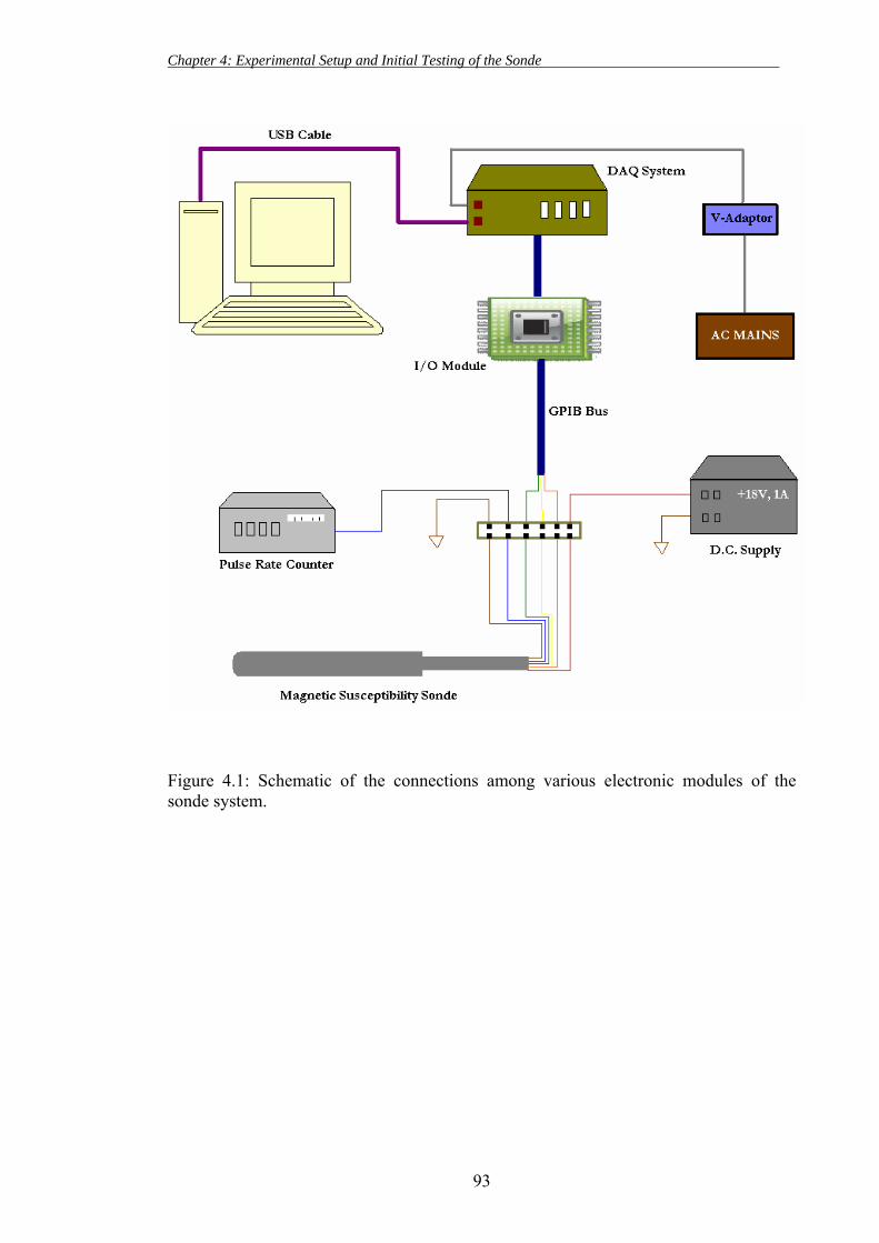
42 Connections and test set-up helliphelliphelliphelliphelliphelliphelliphelliphelliphelliphelliphelliphelliphelliphelliphelliphelliphelliphelliphellip

421 Data acquisition system (DAQ) helliphelliphelliphelliphelliphelliphelliphelliphelliphelliphelliphelliphelliphelliphelliphellip

422 C series IO module helliphelliphelliphelliphelliphelliphelliphelliphelliphelliphelliphelliphelliphelliphelliphelliphelliphelliphelliphelliphellip

423 Data transfer using LabView helliphelliphelliphelliphelliphelliphelliphelliphelliphelliphelliphelliphelliphelliphelliphelliphellip

43 Operating considerations of the sonde helliphelliphelliphelliphelliphelliphelliphelliphelliphelliphelliphelliphelliphelliphelliphellip

21

22

23

24

25

27

31

45

45

45

46

47

51

52

55

56

56

57

60

61

61

61

61

63

63

64

71

71

72

73

73

73

74

vi

Contents

431 Sonde calibration helliphelliphelliphelliphelliphelliphelliphelliphelliphelliphelliphelliphelliphelliphelliphelliphelliphelliphelliphelliphelliphellip

432 Capacitive effects of borehole fluids helliphelliphelliphelliphelliphelliphelliphelliphelliphelliphelliphelliphelliphellip

433 Thermal equilibration helliphelliphelliphelliphelliphelliphelliphelliphelliphelliphelliphelliphelliphelliphelliphelliphelliphelliphellip

434 Referencing helliphelliphelliphelliphelliphelliphelliphelliphelliphelliphelliphelliphelliphelliphelliphelliphelliphelliphelliphelliphelliphelliphelliphellip

435 Pressure and temperature considerations helliphelliphelliphelliphelliphelliphelliphelliphelliphelliphelliphelliphellip

436 Electromagnetic compatibility helliphelliphelliphelliphelliphelliphelliphelliphelliphelliphelliphelliphelliphelliphelliphelliphellip

437 Logging rate helliphelliphelliphelliphelliphelliphelliphelliphelliphelliphelliphelliphelliphelliphelliphelliphelliphelliphelliphelliphelliphelliphellip

44 Prototype performance experiments helliphelliphelliphelliphelliphelliphelliphelliphelliphelliphelliphelliphelliphelliphelliphelliphellip

45 Borehole materials used in my experiments helliphelliphelliphelliphelliphelliphelliphelliphelliphelliphelliphelliphellip

46 Preparation of model boreholes in the laboratory helliphelliphelliphelliphelliphelliphelliphelliphelliphelliphelliphellip

461 Model boreholes from powder material helliphelliphelliphelliphelliphelliphelliphelliphelliphelliphelliphelliphellip

462 Model boreholes from solid rock helliphelliphelliphelliphelliphelliphelliphelliphelliphelliphelliphelliphelliphelliphelliphellip

47 Results of experiments in the model boreholes helliphelliphelliphelliphelliphelliphelliphelliphelliphelliphellip

471 Sonde performance in a 445 mm diameter heterogeneous borehole ndash

Powder samples helliphelliphelliphelliphelliphelliphelliphelliphelliphelliphelliphelliphelliphelliphelliphelliphelliphelliphelliphelliphelliphelliphelliphellip

472 Sonde performance in a 50 mm diameter heterogeneous borehole ndash Solid

rock samples helliphelliphelliphelliphelliphelliphelliphelliphelliphelliphelliphelliphelliphelliphelliphelliphelliphelliphelliphelliphelliphelliphelliphelliphelliphellip

48 Effect of an increase in borehole diameter on sonde performance helliphelliphelliphellip

49 Conclusions helliphelliphelliphelliphelliphelliphelliphelliphelliphelliphelliphelliphelliphellip helliphelliphelliphelliphelliphelliphelliphelliphelliphelliphellip

Chapter 5 Effect of Temperature on Magnetic Susceptibility of Reservoir

Rocks helliphelliphelliphelliphelliphelliphelliphelliphelliphelliphelliphelliphelliphelliphelliphelliphelliphelliphelliphelliphelliphelliphelliphelliphelliphelliphelliphelliphelliphellip


52 Previous studies helliphelliphelliphelliphelliphelliphelliphelliphelliphelliphelliphelliphelliphelliphelliphelliphelliphelliphelliphelliphelliphelliphelliphelliphellip

53 Reservoir samples used in my experiments helliphelliphelliphelliphelliphelliphelliphelliphelliphelliphelliphelliphelliphellip

54 Importance of magnetic hysteresis measurements on reservoir rocks helliphelliphelliphellip

55 Room temperature magnetic hysteresis measurements on reservoir samples hellip

551 Reservoir I samples (P210 and P286) helliphelliphelliphelliphelliphelliphelliphelliphelliphelliphelliphelliphellip

552 Reservoir II samples (P840 P8122 and P813) helliphelliphelliphelliphelliphelliphelliphelliphelliphellip

553 HPHT shallow marine samples (M28 and M68) helliphelliphelliphelliphelliphelliphelliphelliphellip

554 Turbidite samples (175024 176061 and S3) helliphelliphelliphelliphelliphelliphelliphellip

555 Hematite sample (MST1) helliphelliphelliphelliphelliphelliphelliphelliphelliphelliphelliphelliphelliphelliphelliphelliphelliphellip

56 Effect of temperature on magnetic susceptibilities of dia para and

ferromagnetic minerals helliphelliphelliphelliphelliphelliphelliphelliphelliphelliphelliphelliphelliphelliphelliphelliphelliphelliphelliphelliphelliphellip

561 Temperature dependent susceptibility (TDS) analysis on para-ferro

samples (176061 P813) helliphelliphelliphelliphelliphelliphelliphelliphelliphelliphelliphelliphelliphelliphelliphelliphelliphelliphelliphelliphellip

75

75

75

75

75

76

76

76

77

79

79

81

81

81

83

84

85

104

104

105

106

107

107

110

111

111

112

112

112

115

vii

Contents

562 Temperature dependent susceptibility (TDS) analysis on dia-ferro

samples (P84 P286) helliphelliphelliphelliphelliphelliphelliphelliphelliphelliphelliphelliphelliphelliphelliphelliphelliphelliphelliphelliphelliphellip

563 High temperature analysis on dia-antiferro sample (MST1) helliphelliphelliphelliphellip

57 Temperature and depth dependence on magnetic hysteresis parameters

58 Percent susceptibility contribution of the matrix and the ferromagnetic

components helliphelliphelliphelliphelliphelliphelliphelliphelliphelliphelliphelliphelliphelliphelliphelliphelliphelliphelliphelliphelliphelliphelliphelliphelliphelliphelliphellip


Chapter 6 Conclusions Summary of Innovative Aspects and

Recommendations helliphelliphelliphelliphelliphelliphelliphelliphelliphelliphelliphelliphelliphelliphelliphelliphelliphelliphelliphelliphelliphelliphelliphelliphellip


611 System modelling and testing of a magnetic susceptibility sonde system

612 Temperature dependence of the magnetic susceptibility of reservoir rocks

62 Summary of innovative aspects helliphelliphelliphelliphelliphelliphelliphelliphelliphelliphelliphelliphelliphelliphelliphelliphelliphellip

63 Recommendations for future work helliphelliphelliphelliphelliphelliphelliphelliphelliphelliphelliphelliphelliphelliphelliphelliphellip

References helliphelliphelliphelliphelliphelliphelliphelliphelliphelliphelliphelliphelliphelliphelliphelliphelliphelliphelliphelliphelliphelliphelliphelliphelliphelliphelliphellip

119

121

121

125

127

154

154

154

155

157

157

159

viii

List of Tables

List of Tables

11 Effect of clays on downhole logging tools used in hydrocarbon exploration helliphellip

21 Initial mass magnetic susceptibilities of diamagnetic paramagnetic and

compensated antiferromagnetic minerals of petroleum-bearing sediments and

compounds related to the hydrocarbon industry helliphelliphelliphelliphelliphelliphelliphelliphelliphelliphelliphelliphellip

22 Initial mass magnetic susceptibilities of ferromagnetic ferrimagnetic and canted

antiferrimagnetic minerals of petroleum-bearing sediments and compounds related to

hydrocarbon industry helliphelliphelliphelliphelliphelliphelliphelliphelliphelliphelliphelliphelliphelliphelliphelliphelliphelliphelliphelliphelliphelliphelliphelliphellip

23 Single domain-multidomain and superparamagnetic-single domain threshold

sizes of ferrimagnetic and ferromagnetic minerals helliphelliphelliphelliphelliphelliphelliphelliphelliphelliphelliphellip

24 CurieNeel temperatures and common high temperature mineral transformations

of ferromagnetic ferrimagnetic and canted antiferrimagnetic minerals of petroleum-

bearing sediments and compounds related to hydrocarbon industry helliphelliphelliphelliphelliphellip

25 Calculated mass magnetic susceptibility (χm) values for common clay minerals

(para ferri and anti-ferro) at various reservoir temperatures using the Curie-Weiss

law

41 Specifications for the magnetic susceptibility sonde system helliphelliphelliphelliphelliphelliphelliphellip

42 A six wire electrical interface for the magnetic susceptibility sonde system helliphellip

43 Properties of reservoir samples used in my study and their corresponding

magnetic susceptibilities measured on Bartingtonrsquos probe helliphelliphelliphelliphelliphelliphelliphelliphelliphellip

44 Change in sonde output when run in a 445 mm diameter heterogeneous

borehole consisting of CC CI BI and BM layers helliphelliphelliphelliphelliphelliphelliphelliphelliphelliphelliphelliphellip

45 Change in sonde output when run in a 50 mm diameter heterogeneous borehole

consisting layers of Doddington Locharbriggs and Clashach sandstones

helliphelliphelliphelliphellip

46 Effect of decentralization of the magnetic susceptibility sonde on its output

signal inside the borehole helliphelliphelliphelliphelliphelliphelliphelliphelliphelliphelliphelliphelliphelliphelliphelliphelliphelliphelliphelliphelliphelliphellip

51 Summary of the reservoir rock samples used in the study Abbreviation (NM) -

not measured (NK) ndash not known helliphelliphelliphelliphelliphelliphelliphelliphelliphelliphelliphelliphelliphelliphelliphelliphelliphelliphelliphellip

52 Magnetic susceptibility of magnetite and its percent fraction in various domain

states helliphelliphelliphelliphelliphelliphelliphelliphelliphelliphelliphelliphelliphelliphelliphelliphelliphelliphelliphelliphelliphelliphelliphelliphelliphelliphelliphelliphelliphelliphellip

53 Numbers volumes and total surface area of SP SSD and MD magnetite crystals

in a 10cm3 pot of soil with bulk χLfld = 0001times10-6m3kg-1 calculated assuming

10

34

34

35

35

36

88

89

89

90

91

92

129

130

ix

List of Tables

spherical crystals (v=43πr3 a=4πr2) and 50 porosity helliphelliphelliphelliphelliphelliphelliphelliphelliphelliphellip

54 Room temperature magnetic properties of representative reservoir rock samples

55 High temperature magnetic properties of representative reservoir rock samples

at applied fields of 10mT helliphelliphelliphelliphelliphelliphelliphelliphelliphelliphelliphelliphelliphelliphelliphelliphelliphelliphelliphelliphelliphelliphellip

130

131

133

x

List of Figures

List of Figures

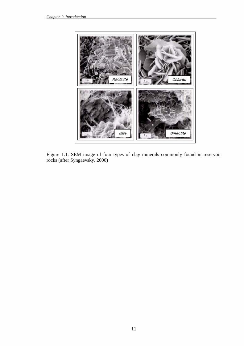
11 Scanning electron microscope (SEM) image of four types of clay minerals

commonly found in reservoir rocks helliphelliphelliphelliphelliphelliphelliphelliphelliphelliphelliphelliphelliphelliphelliphelliphelliphelliphellip

21 Atomicmagnetic behaviour of diamagnetic paramagnetic ferromagnetic

antiferromagnetic and ferrimagnetic classes of substances helliphelliphelliphelliphelliphelliphelliphelliphelliphellip

22 The range of initial mass magnetic susceptibility values (quoted by various

authors) for paramagnetic and compensated antiferromagnetic minerals related to

hydrocarbon reservoirs and their sediment environment helliphelliphelliphelliphelliphelliphelliphelliphelliphelliphellip


authors) for diamagnetic minerals related to hydrocarbon reservoirs and their

sediment environment helliphelliphelliphelliphelliphelliphelliphelliphelliphelliphelliphelliphelliphelliphelliphelliphelliphelliphelliphelliphelliphelliphelliphellip


authors) for ferromagnetic and canted antiferromagnetic minerals related to

hydrocarbon reservoirs and their sediment environment helliphelliphelliphelliphelliphelliphelliphelliphelliphellip

25 SP-SD and SD-MD threshold sizes of ferrimagnetic and canted

antiferromagnetic minerals helliphelliphelliphelliphelliphelliphelliphelliphelliphelliphelliphelliphelliphelliphelliphelliphelliphelliphelliphelliphellip

26 Magnetic hysteresis curve of an assemblage of randomly oriented multidomain

or single domain ferromagnetic minerals helliphelliphelliphelliphelliphelliphelliphelliphelliphelliphelliphelliphelliphelliphelliphellip

27 Comparison of coercivity (HcrHc) and magnetisation (MrsMs) ratios changes

in the domain state of ferromagnetic minerals helliphelliphelliphelliphelliphelliphelliphelliphelliphelliphelliphelliphelliphellip

28 Typical hysteresis loops for samples containing combinations of ferromagnetic

and paramagnetic minerals (ferro+para) antiferromagnetic and diamagnetic minerals

(aferro+dia) and for relatively cleaner paramagnetic and diamagnetic samples helliphellip

29 Theoretically calculated magnetic susceptibility values for different reservoir

minerals at temperatures 20-330 oC using Curie-Weiss law helliphelliphelliphelliphelliphelliphelliphelliphellip

210 Temperature-susceptibility curves of various reservoir rock minerals on a

logarithmic scale helliphelliphelliphelliphelliphelliphelliphelliphelliphelliphelliphelliphelliphelliphelliphelliphelliphelliphelliphelliphelliphelliphelliphelliphelliphellip

211 Experimental thermomagnetic curves and their 2nd derivative measured for

hematite sample MST1 helliphelliphelliphelliphelliphelliphelliphelliphelliphelliphelliphelliphelliphelliphelliphelliphelliphelliphelliphelliphelliphelliphellip

31 A schematic view of the downhole magnetic susceptibility sonde helliphelliphelliphelliphellip

32 Photograph of the prototype magnetic susceptibility sonde helliphelliphelliphelliphelliphelliphelliphellip

33 Core Drive Circuit with Manual Switching helliphelliphelliphelliphelliphelliphelliphelliphelliphelliphelliphelliphelliphellip

34 (a) General form of a 3-pole Bessel filter (b) Bessel filter with real component

values helliphelliphelliphelliphelliphelliphelliphelliphelliphelliphelliphelliphelliphelliphelliphelliphelliphelliphelliphelliphelliphelliphelliphelliphelliphellip

11

37

38

38

39

39

40

40

41

42

43

44

66

67

68

68

xi

List of Figures

35 (a) The electronic circuitry for the magnetic susceptibility sonde system for

providing binary output helliphelliphelliphelliphelliphelliphelliphelliphelliphelliphelliphelliphelliphelliphelliphelliphelliphelliphelliphelliphelliphelliphelliphellip

35 (b) The remaining part of the electronic circuit which provides pulse rate output

from the magnetic susceptibility sonde system helliphelliphelliphelliphelliphelliphelliphelliphelliphelliphelliphelliphelliphelliphellip

41 Schematic of the connections among various electronic modules of the sonde

system helliphelliphelliphelliphelliphelliphelliphelliphelliphelliphelliphelliphelliphelliphelliphelliphelliphelliphelliphelliphelliphelliphelliphelliphelliphelliphelliphelliphelliphellip

42 A print out of the LabView program written for the sonde system helliphelliphelliphelliphellip

43 A computer screen image of the sonde data output helliphelliphelliphelliphelliphelliphelliphelliphelliphelliphellip

44 An increase in frequency of the output waveform when the sonde comes in

contact with a strongly magnetic formation helliphelliphelliphelliphelliphelliphelliphelliphelliphelliphelliphelliphelliphelliphellip

45 Apparatus to prepare model boreholes from powder materials (a) Various parts

of the borehole preparation kit shown individually (b) When parts are put together

46 (a) High pressure assembly for inserting pressure on the powdered samples (b)

Another pressure assembly to remove the central rod out from the borehole sample

47 445 mm internal diameter borehole samples made from powder materials hellip

48 50 mm internal diameter borehole samples made from solid blocks of materials

49 Prototype magnetic susceptibility sonde running inside the 445 mm diameter

samples (from the top BI CI and BM samples) when stacked together in the

borehole formation helliphelliphelliphelliphelliphelliphelliphelliphelliphelliphelliphelliphelliphelliphelliphelliphelliphelliphelliphelliphelliphelliphelliphelliphellip

410 Output from the magnetic susceptibility sonde when run in a 445 mm

diameter heterogeneous reservoir helliphelliphelliphelliphelliphelliphelliphelliphelliphelliphelliphelliphelliphelliphelliphelliphelliphelliphelliphellip


samples (from the top Doddington Locharbriggs and Clashach sandstones) when

stacked together in the borehole formation At the bottom is a solid Locharbriggs

block helliphelliphelliphelliphelliphelliphelliphelliphelliphelliphelliphelliphelliphelliphelliphelliphelliphelliphelliphelliphelliphelliphelliphelliphelliphelliphelliphelliphelliphelliphellip

412 Output from the magnetic susceptibility sonde when run in a 50 mm diameter

heterogeneous reservoir helliphelliphelliphelliphelliphelliphelliphelliphelliphelliphelliphelliphelliphelliphelliphelliphelliphelliphelliphelliphelliphelliphelliphellip

413 A photographic image of the borehole section and the sonde placed in its

center helliphelliphelliphelliphelliphelliphelliphelliphelliphelliphelliphelliphelliphelliphelliphelliphelliphelliphelliphelliphelliphelliphelliphelliphelliphelliphelliphelliphelliphelliphellip


when run in the borehole of Figure 413 helliphelliphelliphelliphelliphelliphelliphelliphelliphelliphelliphelliphelliphelliphelliphelliphellip

51 (a) shows room temperatue hysteresis curves for shoreface reservoir I amp II

samples (P21 P286 P8122 P84 and P813) HPHT shallow marine samples (M68

and M28) turbidite samples (S3 176061 and 175024) and a hematite sample

MST1 (b) shows the magnified hysteresis loops excluding highly paramagnetic

69

70

93

94

95

95

96

97

98

98

99

100

101

102

103

103

xii

List of Figures

turbidite samples (S3 176061 and 175024) helliphelliphelliphelliphelliphelliphelliphelliphelliphelliphelliphelliphelliphellip

52 (a) and (c) represent the magnetic hysteresis loops for shoreface reservoir I

samples (P21 and P286) and shoreface reservoir II samples (P8122 P84 and P813)

respectively Their corresponding ferromagnetic hysteresis loops (b) and (d) are

shown on the right after subtracting the paramagneticdiamagnetic componentshelliphellip

53 (a) and (c) represent the magnetic hysteresis loops for HPHT shallow marine

reservoir samples (M68 and M28) and turbidite samples (S3 176061 and 175024)

Their corresponding ferromagnetic hysteresis loops (b) and (d) are shown on the

right after subtracting the paramagneticdiamagnetic components helliphelliphelliphelliphelliphelliphellip

54 Theoretical magnetic susceptibility versus temperature curves for a mixture of

Illite+Quartz helliphelliphelliphelliphelliphelliphelliphelliphelliphelliphelliphelliphelliphelliphelliphelliphelliphelliphelliphelliphelliphelliphelliphelliphelliphelliphellip

55 Schematic trends and transitions of low field (Lfld) magnetic susceptibility

values from room temperature to +700 oC for different minerals and domains

superparamagnetic (SP) paramagnetic (P) magnetite (MAG Tc 580 oC)

titanomagnetite (TMAG Tc 250 oC) helliphelliphelliphelliphelliphelliphelliphelliphelliphelliphelliphelliphelliphelliphelliphelliphelliphellip

56 Susceptibility versus temperature curves measured at 11mT and 10mT

applied fields for two samples having mainly diamagnetic matrix and a small

ferromagnetic component helliphelliphelliphelliphelliphelliphelliphelliphelliphelliphelliphelliphelliphelliphelliphelliphelliphelliphelliphelliphelliphellip


applied fields for two samples having mainly paramagnetic matrix and a relatively

large ferromagnetic component helliphelliphelliphelliphelliphelliphelliphelliphelliphelliphelliphelliphelliphelliphelliphelliphelliphelliphellip

58 Change in slope with temperature for sample 176061 having a relatively higher


59 Variations in low field (Lfld) ferromagnetic and paramagnetic susceptibilities

with temperature for sample 176061 helliphelliphelliphelliphelliphelliphelliphelliphelliphelliphelliphelliphelliphelliphelliphelliphelliphellip

510 Change in slope with temperature for sample P813 having a small amount of


511 Effect of temperature on ferromagnetic component for sample P813 helliphelliphellip

512 Variations in low field ferromagnetic and paramagnetic susceptibilities with

temperature for sample P813 helliphelliphelliphelliphelliphelliphelliphelliphelliphelliphelliphelliphelliphelliphelliphelliphelliphelliphelliphelliphellip

513 Experimental low field and ferromagnetic susceptibility (χLfld and χferro)

versus temperature curves for samples having a paramagnetic matrix and the


514 Experimental paramagnetic susceptibility (χpara) versus temperature curves for

reservoir samples having a paramagnetic matrix and a small ferromagnetic

134

135

136

137

137

138

139

140

140

141

141

142

142

xiii

List of Figures

component helliphelliphelliphelliphelliphelliphelliphelliphelliphelliphelliphelliphelliphelliphelliphelliphelliphelliphelliphelliphelliphelliphelliphelliphelliphelliphelliphellip

515 Hysteresis curves for samples P286 and P84 helliphelliphelliphelliphelliphelliphelliphelliphelliphelliphelliphellip

516 Sample P84 has a higher diamagnetic component whereas sample P286

contain paramagnetic impurities which can be seen by a lower magnitude

diamagnetic susceptibility curve for sample P286 helliphelliphelliphelliphelliphelliphelliphelliphelliphelliphelliphellip

517 Change in high field slope with temperature for samples P84 and P286 helliphellip

518 Changes in ferromagnetic hysteresis loops with temperature for sample P84


520 Formation of a new ferromagnetic component in sample P286 at high

temperatures helliphelliphelliphelliphelliphelliphelliphelliphelliphelliphelliphelliphelliphelliphelliphelliphelliphelliphelliphelliphelliphelliphelliphelliphelliphelliphellip


versus temperature curves for samples having mainly diamagnetic matrix and a

small ferromagnetic component helliphelliphelliphelliphelliphelliphelliphelliphelliphelliphelliphelliphelliphelliphelliphelliphelliphelliphellip

522 Experimental diamagnetic susceptibility (χdia) versus temperature curves for

samples shown in Figure 521 helliphelliphelliphelliphelliphelliphelliphelliphelliphelliphelliphelliphelliphelliphelliphelliphelliphelliphelliphellip

523 Changes in the slope of hysteresis curve with temperature for sample MST1

having an anti-ferromagnetic component (hematite) and a diamagnetic matrix

(quartz) helliphelliphelliphelliphelliphelliphelliphelliphelliphelliphelliphelliphelliphelliphelliphelliphelliphelliphelliphelliphelliphelliphelliphelliphelliphelliphelliphelliphellip

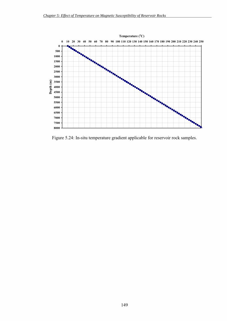
524 In-situ temperature gradient applicable for reservoir rock samples helliphelliphelliphellip

525 (a) and (b) represent the saturation magnetization (Ms) and saturation

remanent magnetization (Mrs) for samples P813 176061 and P84 respectively (c)

and (d) show the corresponding coercivity (Hc) and coercivity of remanence (Hcr)

values for the three samples helliphelliphelliphelliphelliphelliphelliphelliphelliphelliphelliphelliphelliphelliphelliphelliphelliphelliphelliphelliphellip

526 Dependence of remanence ratios with depth for samples P813 176061 and

P84 helliphelliphelliphelliphelliphelliphelliphelliphelliphelliphelliphelliphelliphelliphelliphelliphelliphelliphelliphelliphelliphelliphelliphelliphelliphelliphelliphelliphelliphelliphellip

527 Dependence of coercivity ratios with depth for the representative sediment

samples helliphelliphelliphelliphelliphelliphelliphelliphelliphelliphelliphelliphelliphelliphelliphelliphelliphelliphelliphelliphelliphelliphelliphelliphelliphelliphelliphelliphellip

528 Coercivity ratio HcrHc versus remanence ratio MrsMs for respective

temperature intervals for shoreface samples P813 P84 P286 HPHT sample M28

and turbidite samples 175024 176061 helliphelliphelliphelliphelliphelliphelliphelliphelliphelliphelliphelliphelliphelliphelliphellip

529 Percent susceptibility contribution of individual minerals (diamagnetic

paramagnetic ferromagnetic) towards total magnetic susceptibility (χLfld) signal for

all the studied reservoir samples helliphelliphelliphelliphelliphelliphelliphelliphelliphelliphelliphelliphelliphelliphelliphelliphelliphelliphelliphellip

143

144

144

145

146

146

147

147

148

148

149

150

151

151

152

153

xiv

List of Illustrations


21 The Variable Field Translation Balance (VFTB) helliphelliphelliphelliphelliphelliphelliphelliphelliphelliphellip

31 CAD diagram of the custom made hollow adaptor used to connect the sonde to

the wireline helliphelliphelliphelliphelliphelliphelliphelliphelliphelliphelliphelliphelliphelliphelliphelliphelliphelliphelliphelliphelliphelliphelliphelliphelliphelliphelliphellip

32 Schematic diagram showing the output pulses of monostable multivibrators and

are representative of the magnetic susceptibility signal

24

52

60

xv

List of Abbreviations

List of Abbreviations AC

AMS oC

DAC

DAQ

DC

EM

FWHM

H

Hc

Hcr

HPHT

IC

IO

IRM

K

LED

LTO

M

MD

Mrs

Ms

Msp

NI

NRM

PCB

ppm

PSD

SD

SEM

SI

SIRM

SNR

Alternating Current

Anisotropy of Magnetic Susceptibility

Degree Celsius

Digital-to-Analog Converter

Data Acquisition System

Direct Current

Electromagnetic

Full Width Half Maximum

Magnetic Field Strength

Coercivity of Magnetisation (Coercive Force)

Coercivity of Remanent Magnetisation

High Pressure High Temperature

Integrated Circuit

Input-Output

Isothermal Remanent Magnetisation

Kelvin Potassium

Light Emitting Diode

Low Temperature Oxidation

Magnetisation

Multi-Domain

Saturation Remanent Magnetisation

Saturation Magnetisation

Spontaneous Magnetisation

National Instruments

Natural Remanent Magnetisation

Printed Circuit Board

Parts Per Million

Pseudo-Single Domain

Single-Domain

Scanning Electron Microscope

Systems International

Saturation Isothermal Remanent Magnetisation

Signal to Noise Ratio

xvi


SP

Tc

TDS

TN

USB

VFTB

XRD

Super-Paramagnetic

Curie Temperature

Temperature Dependent Susceptibility

Neacuteel Temperature

Universal Serial Bus

Variable Field Translation Balance

X-ray Diffraction

χ MS Magnetic Susceptibility

χm χ Mass Magnetic Susceptibility

χv κ Volume (bulk) Magnetic Susceptibility

χo Initial Magnetic Susceptibility

χHfld Hfld MS High Field Magnetic Susceptibility

χLfld Lfld MS Low Field Magnetic Susceptibility

χferro Ferromagnetic Susceptibility

χdia Diamagnetic Susceptibility

χpara Paramagnetic Susceptibility

χM Molar Magnetic Susceptibility

μT Micro-Tesla

θ paramagnetic Curie temperature

μr Relative Permeability of the Specimen

μ0 Permeability of Free Space

φ Magnetic Flux

B Magnetic Flux Density

real Reluctance of the Magnetic Circuit

xvii

Chapter 1

Introduction

In all worldwide petroleum basins shaley sand analysis has always challenged

geologists engineers and petrophysicists The main challenge is to identify from cores

or logs the degree to which the clay minerals affect the reservoir quality which is an

important factor in determining the reservoir pay zones For example illite is an

important clay mineral particularly with respect to studies of fluid flow Small increases

in its occurrence can dramatically affect the permeability and microporosity of a sample

by bridging pore space and creating microporous rims A 1-2 increase in the content

of authigenic illite can cause a decrease in permeability of about 2-3 orders of

magnitude without significantly affecting the porosity (Ivakhnenko and Potter 2006)

Even though a reservoir rock looks solid to the naked eye a microscopic examination

reveals the existence of tiny openings in the rock which may help the fluid flow

(Leonardon 1961) It is possible to have a very high porosity without any permeability

at all as in the case of compacted shales The reverse of high permeability with a low

porosity might also be true eg in microfractured carbonates Therefore it is imperative

to know the types of clay minerals and their relative percentages in the reservoir rock

matrix

The petrophysics group at the Institute of Petroleum Engineering Heriot-Watt

University has shown strong correlations between laboratory based magnetic

susceptibility data of reservoir rock minerals with key petrophysical parameters

including permeability (Potter 2005) Therefore it will be extremely useful to develop

a downhole magnetic susceptibility logging sonde which can predict the magnetic

behaviour of most common reservoir clay minerals at in-situ conditions The magnetic

signal obtained downhole can then be used as an indirect indicator of fluid permeability

The testing of the downhole magnetic susceptibility sonde and modeling the magnetic

behaviour of clay minerals at reservoir conditions has been the main subject of this

thesis

1

Chapter 1 Introduction


logging tools

Most of the shaley sand evaluation methods require knowledge of the amount of shales

or clays present in the formation material and how they affect the measurements of

various logging tools Over the years the term lsquoclaysrsquo and lsquoshalesrsquo have been used

interchangeably not because of the lack of understanding but due to different ways in

which properties are measured Clays are defined in terms of both particle size and

mineralogy In terms of size clays refer to particle diameter sizes less than 24mm

Clays are often found in sandstones siltstones and conglomerates The most common

types of clay minerals found in sedimentary rocks are kaolinite chlorite illite and

smectite The scanning electron microscope (SEM) image of these four clay types is

shown in Figure 11 (Syngaevsky 2000) The major effects of clays in a hydrocarbon

reservoir are 1) reduction of effective porosity and permeability 2) migration of fines

whenever clay minerals turn loose migrate and plug the pore throats that cause further

reduction in permeability 3) water sensitivity whenever clays start to hydrate and swell

after contact with water (or mud filtrate) which in turn causes reduction in effective

porosity and permeability 4) acid sensitivity-whenever acid reacts with iron-bearing

clays to form a gelatinous precipitate that clogs pore throat and reduce permeability

Shales are a mixture of clay minerals and other fine grained particles deposited in very

low energy environments They can be distributed in sandstone reservoirs in three

possible ways (1) laminar shale where shale can exist in the form of laminae between

layers of clean sand (2) structural shale where shale can exist as grains or nodules

within the formation matrix and (3) dispersed shale where shale can be dispersed

throughout the sand partially filling the intergranular interstices or can be coating the

sand grains All these forms can occur simultaneously in the same formation Each form

can affect the amount of rock porosity by creating a layer of closely bound surface

water on the shale particle

The presence of clay minerals or shale affects the responses of the majority of logging

tools For example they can generally cause a higher reading of apparent porosity

indicated by density neutron and sonic tools and a suppressed reading by resistivity

tools This is because in density tools the presence of clay minerals lowers the apparent

density and this causes an increase in the apparent porosity of the tool Also there is a

limitation of tool calibration whenever clay minerals are present In neutron tools the

2


higher concentration of hydrogen ions in clays translate to a higher calculated porosity

whereas in sonic tools the interval transit time of clays is high which corresponds to a

higher porosity In electric logs the clay minerals because of their large surface area

absorb a large quantity of reservoirrsquos pore water to their surface This bound water

contributes to additional electrical conductivity hence lowering the resistivity Table 11

shows a list of various logging tools their method of operation and how their

performance is affected by the presence of clay minerals

12 Clay magnetism and its significance in reservoir characterization

The major constituents of many sedimentary rocks usually quartz in sandstones or

calcite in carbonates are represented by a low and negative magnetic susceptibility I

will explain the magnetic susceptibility term in Section 26 Chapter 2 On the other

hand permeability controlled by clays like illite is represented by a low and positive

magnetic susceptibility Therefore by simply looking at the magnetic susceptibility

signal (positive or negative) one can tell whether there are paramagnetic clay minerals

present in the reservoir rock

And this is certainly a good guide to explaining the relative magnitudes of

susceptibilities in samples of pure minerals However it is uncommon for a natural

sample to contain only one category of magnetic minerals For instance the presence of

iron bearing minerals also gives a high and positive magnetic susceptibility It is

therefore necessary to consider virtually all samples as a mixture of minerals often

falling into two or three categories of magnetic behaviour and each having a different

magnetic susceptibility value The idea of interpreting each measurement in terms of

many different minerals sounds a fairly daunting task But in practice we can simplify

matters by making some assumptions about which minerals are significant in a sample

Samples which are not contaminated by ferrous metal do not usually contain iron

bearing minerals In their absence the susceptibility of a sample is most likely to be

controlled by other paramagneticdiamagnetic minerals


susceptibility sonde

Historically the development of magnetic studies for hydrocarbon application was

restricted to magnetic prospecting (Donovan et al 1979) and petrophysical

investigations for the detection of oil and gas reservoirs (Bagin et al 1973 Bagin and

3


Malumyan 1976) Magnetic techniques utilizing the Earthrsquos magnetic field or the

natural remanent magnetisation (NRM) in the reservoir rocks also played a prominent

role in petroleum reservoir exploration and research High resolution magnetic surveys

(Eventov 1997 2000) utilize the present Earthrsquos magnetic field Such survey tools

measure three orthogonal components of the local magnetic fields and from these data

the toolrsquos inclination azimuth and toolface orientation can be calculated Also

boreholes are commonly surveyed for drilling using the Earthrsquos magnetic field as a

north reference (Wilson and Brooks 2001)

Palaeomagnetism together with standard magnetostratigraphy is starting to be used for

correlation purposes in the petroleum industry (Gillen et al 1999 Cioppa et al 2001

Filippycheva et al 2001) NRM in palaeomagnetism is a key parameter for the

orientation of directional properties to geographic coordinates (Hailwood and Ding

1995) and helping to date hydrocarbons (Symons et al 1999) Environmental

magnetism is also an important discipline for the detection of hydrocarbon seepage

(Yeremin et al 1986 Liu et al 1996 Costanzo-Alvarez et al 2000) and

contamination (Cogoini 1998)

A variety of techniques have been used in the past to measure the magnetic properties of

minerals including fractionation with a magnetic separator (Stradling 1991) Frantz

isodynamic separator (Nesset and Finch 1980 and McAndrew 1957) magnetometer

(Foner and McNiff 1968 and Lewis and Foner 1976) SQUID (Sepulveda et al 1994)

resonant coil (Cooke and De Sa 1981 and Isokangas 1996) and the inductance bridge

(Drobace and Maronic 1999 Stephenson and De Sa 1970 Foner 1991 and Tarling and

Hrouda 1993) These techniques are generally considered laboratory methods due to

the length of time required to process the samples

The developments in instrumentation and software with time have attracted a number

of scientists towards the application of magnetic susceptibility methods in the

hydrocarbon industry They include magnetic susceptibility studies and its integration

with magnetometer and other surface geophysical surveys and with soil magnetic

studies accomplished in the laboratory However some still think that there will be

insufficient contrast in the magnetic susceptibility of sand and gravel compared to clays

and other sedimentary rocks in order to differentiate those (Jeffrey et al 2007)

4


The development of industrial grade equipment to measure magnetic susceptibility was

identified by the Julius Kruttschnitt Mineral Research Centre (JKMRC) This equipment

is able to measure complex magnetic susceptibility (ie both phase and amplitude of the

magnetic susceptibility vector) from 10 Hz to 100 kHz at infinitely adjustable field

strengths (Cavanough and Holtham 2001 and Cavanough and Holtham 2004) The CS-

2 and KLY-2 Kappabridge was used for the measurement of thermal changes of

magnetic susceptibility in weakly magnetic rocks (Hrouda 1994) Low field variation

of magnetic susceptibility was used to see its effect on anisotropy of magnetic

susceptibility (AMS) (Hrouda 2002) Magnetic susceptibility and AMS together with

the intensity inclination and declination of the natural remanent magnetisation have

formed the basis of high resolution rock magnetic analyses (Hall and Evans 1995 Liu

and Liu 1999 Robin et al 2000)

At present certain magnetic methods are becoming more recognised and applied within

the petroleum industry in particular using magnetic susceptibility measurements to

predict petrophysical properties such as clay content and permeability (Potter 2004a

Potter 2004b Potter et al 2004 Potter 2005 Potter 2007 Ivakhnenko and Potter

2008 Potter and Ivakhnenko 2008) However all these methods are laboratory based

and the downhole magnetic susceptibility measurements remain a relatively unexploited

tool There are no commercially available downhole magnetic susceptibility logging

tools for industry diameter boreholes as these measurements are not currently part of oil

and gas industry wireline logging or measurements while drilling operations

Therefore one of the aims of this thesis is to build a prototype magnetic susceptibility

sonde capable of measuring the magnetic susceptibility of the formation downhole The

new sonde will be a modernized version of the existing electromagnetic (EM) well-

logging tools The EM tools refer to the process of acquiring information of the earth

formation properties (mainly resistivityconductivity) by taking into account the effect

of eddy currents (Liu et al 1989) In practice the conductivity signal measured by the

EM tools is also affected by the magnetic susceptibility of the formation material

(Fraser 1973) The influence of magnetic susceptibility on EM data has long been

known but very little has been done about its importance towards oil and gas

explorations In most cases magnetic susceptibility has been treated as a source of

contamination in the conductivity signal and people have been trying very hard to

eliminate that contamination by various techniques In doing so useful information

5


about the magnetic susceptibility is wasted and also the recovered conductivity models

become less reliable The magnetic susceptibility sonde in this thesis will suppress the

conductivity signal with the help of various electronic modules such that the

susceptibility signal will overshadow the conductivity signal

14 Research Objectives

This dissertation has three main objectives The first objective is the system modeling

and testing of a demonstration version of the downhole sonde capable of taking raw

magnetic susceptibility measurements in-situ conditions This includes the susceptibility

contributions from all the reservoir rock minerals which are present within the vicinity

of the sensor coil in the sonde The susceptibility signal will potentially aid in the

interpretation of the main lithological zonations inside the borehole at high resolution

Since the petrophysics research group at HW University has demonstrated correlations

between the magnetically derived mineral contents and petrophysical parameters

(permeability the cation exchange capacity per unit pore volume and the flow zone

indicator) the downhole magnetic susceptibility signal can potentially provide in-situ

predictions of these parameters The cut-offs between the different lithologies could be

quantitatively more accurate than the gamma ray tool due to the higher potential

resolution of the magnetic sonde The proposed sonde would operate at oil or gas

reservoir temperatures (up to at least 110deg C) and pressures of around 6000 ndash 10000 psi

(about 40 ndash 70 MPa) This would make downhole in-situ measurements of magnetic

susceptibility as part of a wireline logging string Possibly it may also be incorporated

in another form of downhole measurements these being measurements while drilling

(MWD)

The second objective of this dissertation is to create some model boreholes in the

laboratory and to test the working of the prototype downhole sonde on these boreholes

at normal conditions of temperature and pressure The heterogeneous boreholes will

contain layers of relatively clean sand confined and dispersed clay and some shaley

material The prototype magnetic susceptibility sonde should be able to pick up bed

boundaries and to distinguish various types of layers based on their magnetic

susceptibility values

The third objective is to study the temperature dependence of magnetic susceptibility on

reservoir rocks in order to determine magnetic susceptibilities at reservoir conditions

6


Thermomagnetic analyses on a number of reservoir samples is carried out (to model the

in-situ conditions for the downhole sonde) to investigate the effect of increase in

temperature on their low and high field magnetic susceptibilities hysteresis parameters

domain state etc This would help to model the effect on the output of downhole

susceptibility sonde at in-situ conditions

15 Organization of the Dissertation

Chapter 1 is the introductory chapter emphasizing how shaleyclay rich formations

give rise to a higher magnetic susceptibility signal than clean formations It briefly

explains how shaley formations affect the performance of various logging tools and the

importance of magnetic susceptibility data which is obtained as a byproduct from the

conductivity tool It also briefly outlines previous work on various magnetic techniques

in the petroleum industry

Chapter 2 describes general aspects of rock and mineral magnetism It outlines various

classes of clay minerals in terms of their magnetic behaviour The magnetic properties

like domain states and magnetic hysteresis are explained in terms of mineral grain size

and magnetic phase The main challenge in this chapter is to identify the degree to

which the clay minerals affect the susceptibility signal For this I have compiled and

presented in tabular form the magnetic susceptibility data for a range of

mineralsmaterials from existing literature Towards the end of this chapter

thermomagnetic analysis of the magnetic susceptibility signal is explained which forms

the basis of Chapter 5

Chapter 3 explains the step by step procedure for the design and modeling of the

prototype magnetic susceptibility sonde system This includes the design of the

electronic circuit coil system the housing to hold the printed circuit board (PCB) and

the coils and the shielding system to protect the sonde from the borehole environment

This chapter also explains a detailed mathematical analysis of the sonde operation

output data formats and the type of wireline used

Chapter 4 explains the performance of the sonde system as a whole It involves

interaction among the sonde various electronic modules and the personal computer It

also demonstrates how the connections are carried out between the sonde and the data

acquisition system (DAQ) The experimental setup on initial testing of the magnetic

7


8

susceptibility sonde and the transfer and processing of the susceptibility data using

LABVIEW software is also explained in this chapter

Chapter 5 describes laboratory based thermomangetic analyses on a number of

different reservoir rock samples (shoreface shallow marine (high pressure high

temperature) and turbidite) In particular the effect of variation in grain size and

magnetic mineralogy is analysed with respect to variation in temperature Hysteresis

parameters are shown to be a powerful tool for identifying multiple domain states and

changes in mineralogy in a reservoir rock sample I have used the variations of magnetic

susceptibility with temperature to model the in-situ reservoir conditions I have also

performed temperature dependent susceptibility (TDS) measurements to quantify

mineralogy

The main conclusions drawn from the different sections of this thesis are reported in

Chapter 6 All innovative aspects of the thesis and recommendations for further work

are also summarised in this chapter


9

Tool Designation

Measurement Applications Limitations Effect of Clays on Tool Performance

Induction logging

Dual induction

DIL

Formation resistivity in oil-

based muds or air-drilled

boreholes

Determine Sw can be used

in oil based or fresh water

muds Focused to minimize

the influence of the

borehole

Difficult to calibrate

lower vertical resolution

not ideal for mapping

confined fractures

Clays cause an increase in magnetic

susceptibility signal which is

superimposed on the conductivity

signal and so tool gives a higher

output

Gamma ray GR

Records naturally occurring

gamma radiations from the

formation

Detection of radioactive

minerals estimate shale in

dirty sands shale vs non-

shale and shale content

Not very suitable for well

to well correlations and

also in KCL based

drilling muds

Presence of clays causes a higher

output signal from the gamma ray

tool

Sonic

Borehole

compensated

Long spaced sonic

BHC

LSS

Measures the transit time of

acoustic waves through the

formation rock

Detection of fractures

lithology and porosity

prediction

May cause problems

when tool is run at

shallower depths for large

diameter boreholes

doesnrsquot detect secondary

porosity

The transit time of clays is higher

The tool gives a higher value of

apparent porosity

Compensated

neutron log

CNL Impact of neutrons on H

atoms within the formation

Determination of porosity

correlation lithology and

gas detection

Cannot be used in gas-

filled boreholes

High concentration of hydrogen

ion in clays translate to a higher

calculated porosity

The tool is sensitive to shales which

contain boronrare-earth elements

with a high thermal neutron capture

hapter 1 Introduction

10

Normal resistivity

logs

Short normal

Long normal

Lateral

SN

LN

LAT

Formation resistivity Determine Sw porosity

severe invasion effect

Cannot be used in non-

conductive muds

Bound water in clays reduces the

resistivity signal

Density

Compensated

formation density

Litho-Density tool

FDC

LDT

Impact of gamma rays on

electrons in the formation

Measurement of porosity

bulk density seismic

velocity identification of

minerals in complex

lithology nature of fluid in

pores gas detection

Borehole size correction

is required

Clay has lower density (higher

apparent porosity) than quartz

Spontaneous

potential

SP Measures naturally

occurring potentials in the

well bore as a function of

depth

Detection of permeable

zones determination of

formation water salinity

and bed thicknesses


conductive or oil-based

muds

Bound water in clays contributes

to additional electrical

conductivity or lower resistivity

Microresistivity

logs

Microlaterolog

Proximity log

MLL

PL

Resistivity of the

invadedflushed zone

Determine Sw identify

permeable formations can

be used to correct deep

resistivity measurements

Quantitative inference of

permeability is not

possible poor if thick

mudcake poor if shallow

invasion


resistivity signal

Table 11 Effect of clays on downhole logging tools used in hydrocarbon exploration

C


Figure 11 SEM image of four types of clay minerals commonly found in reservoir rocks (after Syngaevsky 2000)

11

Chapter 2

Introduction to Magnetic Susceptibility of Rocks and Minerals Found

in Hydrocarbon Reservoirs

21 Brief synopsis

This chapter provides an overview of the main magnetic properties of rocks and

minerals found in hydrocarbon reservoirs and also highlights the advantages of

measuring their magnetic susceptibility signal It describes the laboratory based method

for measuring the magnetic susceptibility of reservoir rocks at various temperatures and

the importance of susceptibility versus temperature curves in characterizing the

reservoir rock matrix The description will lay the basis for the importance of the

magnetic susceptibility sonde designed in Chapter 3 and the thermomagnetic analysis

of magnetic susceptibility explained in Chapter 5 of this thesis To understand the

importance of magnetic susceptibility the magnetic properties and main magnetic

classes of reservoir rocks and minerals are described in relation to their applicability to

the petroleum industry The magnetic analyses covered in this chapter include magnetic

susceptibility magnetic hysteresis and thermomagnetic measurements

22 Classes of clay minerals based on their magnetic behaviour

A mineral or material is classified as magnetic if it gives rise to magnetic induction in

the presence of a magnetic field The magnetization (M) of the material is related to the

applied field strength (H) by the equation

M = χH (21)

where χ is the magnetic susceptibility of the material It is a dimensionless quantity

which expresses the ease with which a substance may be magnetized Magnetic

susceptibility is a very important physical parameter in exploration geophysics and

information about its distributions can be used to determine subsurface structures and

to detect mineral deposits and other natural resources All substances universally exhibit

magnetic susceptibility at temperatures above absolute zero (Tarling and Hrouda 1993)

12

Chapter 2 Magnetic Susceptibility of Rocks and Minerals Found in Hydrocarbon Reservoirs

Magnetic susceptibility data for minerals present in sediments has been reported by a

number of authors (Foex et al 1957 Mullins 1977 Collinson 1983 Hunt et al 1995

Matteson et al 2000) although the data is by no means comprehensive The most

extensive single literature source is Hunt at al (1995) Another useful source of relative

and indirect magnetic susceptibility values is given by Rosenblum and Brownfield

(1999) I therefore collected and recalculated where necessary all available literature

data of magnetic susceptibility for relevant sediment minerals and these values are

given in Tables 21 and 22 The data shows that all minerals can be classified in terms

of their magnetic behaviour falling into one of the five categories diamagnetism

paramagnetism ferromagnetism ferrimagnetism and antiferromagnetism

221 Diamagnetism

Diamagnetism is shown by the materials whose outermost shells are completely filled

with electrons On the application of an external magnetic field the spin of the electrons

andor their orbital angular momentum changes This makes the electrons to precess and

oppose the external applied field In other words diamagnetic materials cause a

reduction in the strength of the external applied field the reason diamagnetic materials

show negative magnetic susceptibilities Diamagnetic susceptibility is usually very

weak and only those atoms with completely filled orbits show diamagnetic effect

(Butler 1992) The susceptibility of a diamagnetic material is given by the equation

(Spaldin 2003)

av2

e

20 )(r

6mZeNμχ minus= (22)

where N is the number of atoms per unit volume μ0 is the permeability of free space (a

free atom is considered) r is the orbital radius of the electrons Z is the total number of

electrons e is the charge and me is the mass of electron Also note from the equation

that the susceptibility lsquoχrsquo is dimensionless and also negative and that there is no explicit

temperature dependence However the amount of magnetization is proportional to

(r2)av which is very weakly temperature dependent

The plot of magnetization (M) versus applied field (H) gives the curve shown in Figure

21a Pure quartz calcite and feldspar are examples of diamagnetic minerals and are

characterized by having negative magnetic susceptibilities in the order of -10-6 SI in

13


terms of volume susceptibility (Hrouda 1973 and Borradaile et al 1987 as reported by

Borradaile 1988) However these minerals are rarely pure as they commonly contain

non-diamagnetic inclusions

Since diamagnetic materials show negative magnetic susceptibilities whereas

paramagnetic materials show positive magnetic susceptibilities the alloys of

diamagnetic and paramagnetic materials can be used in delicate magnetic measurements

(Spaldin 2003) This is due to the fact that a particular composition of diamagnetic and

paramagnetic minerals can be used to have net zero magnetic susceptibility at a

particular temperature

222 Paramagnetism

In this class of materials the atoms or ions have a net magnetic moment due to unpaired

electrons in their partially filled orbits However the individual magnetic moments do

not interact magnetically (Figure 21b) In transition metal salts the cations have

partially filled d shells and the anions cause separation between cations This weakens

the magnetic moments on neighboring cations (Spaldin 2003) The Langevin model

states that each atom has a magnetic moment which is randomly oriented as a result of

thermal energies (Langevin 1905) Therefore in zero applied magnetic field the

magnetic moments point in random directions When a field is applied a partial

alignment of the atomic magnetic moments in the direction of the field results in a net

positive magnetization and positive susceptibility (Tarling 1983) At low fields the

flux density within a paramagnetic material is directly proportional to the applied field

so the susceptibility χ = MH is approximately constant Unless the temperature is very

low (ltlt100 K) or the field is very high paramagnetic susceptibility is independent of

the applied field (Moskowitz 1991)

Most iron bearing carbonates and silicates are paramagnetic Many salts of transition

elements are also paramagnetic At normal temperatures and in moderate fields the

paramagnetic susceptibility is small However the strength of paramagnetic

susceptibility depends on the concentration of paramagnetic minerals present in the

sample In most cases it is larger than the diamagnetic susceptibility contribution In

samples containing ferromagneticferrimagnetic minerals the paramagnetic

susceptibility contribution can only be significant if the concentration of

ferromagneticferrimagnetic minerals is very small In this case a paramagnetic

14


correction may be needed For common paramagnetic rock forming minerals the

paramagnetic susceptibility generally ranges between 10-2 to 10-4 SI vol (Dunlop and

ozdemir 1997)

223 Ferromagnetism

The atomic magnetic moments in ferromagnetic materials exhibit very strong

interactions resulting in a parallel or antiparallel alignment of their magnetic moments

This produces a strong magnetization even in the absence of an applied magnetic field

(Figure 21c) In 1907 Weiss postulated this effect by the presence of a molecular field

within the ferromagnetic material He suggested that magnetic materials consists of

small regions called magnetic domains within which all the atomic magnetic moments

are aligned in the same direction (domain saturation magnetisation) On the application

of an external applied field the response of these magnetic domains to the applied field

determines the magnetic susceptibility of the material (Petty 2007)

In quantum mechanics the Heisenberg model of ferromagnetism describes the parallel

alignment of magnetic moments in terms of an exchange interaction between

neighboring moments (Kennedy 1985) As opposed to paramagnetic materials the

magnetization in ferromagnetic materials is saturated in moderate magnetic fields and at

high temperatures Therefore ferromagnetic materials are usually compared in terms of

saturation magnetization (magnetization when all domains are aligned) rather than

susceptibility

There are numerous ferromagnetic materials present in reservoir rocks and the Fe-Ti

oxides form the majority of them by far Other mineral groups or minerals exhibiting

ferromagnetic properties include goethite (an iron oxyhydroxide) pyrrhotite greigite

(iron sulphides) and hydrated iron sulphate which results from the hydration of pyrite

and marcasite (a relatively unstable minerals when exposed to air) All these minerals

have characteristically high magnetic susceptibilities (greater than paramagnetic

minerals) ranging anywhere from 10-3 SI vol to 100 SI vol (Carmichael 1982 as

reported by Borradaile 1988)

As ferromagnetic materials are heated the thermal agitation of the atoms implies that

the degree of alignment of the atomic magnetic moments decreases and hence the

saturation magnetization also decreases Eventually the thermal agitation becomes so

15


great that the material becomes paramagnetic The temperature of this transition is

called the Curie temperature Tc (for iron Fe Tc =770 degC for cobalt Co Tc =1131 degC

and for nickel Ni Tc =358 degC) Above the Curie temperature the susceptibility varies

according to the Curie-Weiss law The temperature dependence of magnetic

susceptibility for various types of reservoir minerals is explained in Section 262

224 Ferrimagnetism

Ferrimagnetism is only observed in compounds which have more complex crystal

structures than pure elements The exchange interactions enable the parallel alignment

of atomic magnetic moments in some parts of the crystal and anti-parallel alignment in

others (Figure 21d) These break down the material into magnetic domains (see Section

24 for detailed explanation of magnetic domains) Ferrimagnetic materials are very

similar to ferromagnetic materials in terms of spontaneous magnetization Curie

temperatures coercivity hysteresis and remanence After the applied magnetic field is

removed ferromagnetic and ferrimagnetic materials acquire and retain remanent

magnetisation Magnetite is an example of a ferrimagnetic material

225 Antiferromagnetism

In antiferromagnetic materials the exchange interactions causes the antiparallel

alignment of the atomic magnetic moments (Figure 21e) This is in contrast with

ferromagnetic materials where the atomic magnetic moments are aligned in parallel If

the magnitude of atomic magnetic moments is equal and they are completely opposite in

direction this will result in a net zero spontaneous magnetization and the material is a

perfectly compensated antiferromagnetic Such materials have zero remanence no

hysteresis and a small positive susceptibility that varies in a peculiar way with

temperature Ilmenite is such an example (OrsquoReilly 1984)

If the cancelling of the magnetic moments is not complete a small net moment is

observed and the system is described as imperfect antiferromagnetism This imbalance

can have a number of possible origins such as lattice defects crystal impurities or the

spin-canting when the cation-anion-cation exchange bonds are slightly tilted (lt 1o) or

canted Canted antiferromagnetism exhibit the typical magnetic characteristics of

ferromagnetic and ferrimagnetic materials Hematite is an example of a canted

antiferromagnetic mineral (Dunlop and Ozdemir 1997)

16


Unlike ferromagnetic materials which show paramagnetic behaviour above their Curie

temperature the antiferromagnetic materials show paramagnetic behaviour above Neacuteel

temperature (TN) The paramagnetic behavoiur is indicated with a negative intercept

indicating negative exchange interactions (Moskowitz 1991) In the periodic table the

only element exhibiting antiferromagnetism at room temperature is chromium (TN =37

ordmC)

For convenience in the text I will often use the term ferromagnetic to describe

ferromagnetic ferrimagnetic and canted antiferromagnetic substances in this thesis

23 Common minerals found in hydrocarbon reservoir sediments

The most common clay minerals and compounds relevant for petroleum reservoirs and

their initial mass magnetic susceptibilities are shown in Tables 21 and 22 The main

clays are chlorite illite (paramagnetic) kaolinite (diamagnetic) etc While

ferromagnetic minerals (magnetite titanomagnetite maghemite pyrrhotite etc) contain

large concentrations of iron (oxides and sulphides) paramagnetic minerals contain

much smaller concentrations among the diamagnetic cations and anions Therefore a

sample of rock or soil containing predominantly ferromagnetic minerals will give a

much higher susceptibility than one containing say all paramagnetic minerals

Magnetite for instance is about 1000 times more magnetic than one of the strongest

paramagnetic minerals (siderite for example) and about 10000 times stronger than the

weakest clay minerals (illite for example) Hematite being a canted antiferromagnetic

mineral exhibits susceptibility values close to that of strong paramagnetic minerals

(siderite Figure 24)

The paramagnetic minerals (a few of them are shown in Table 21 and Figures 22 and

24) include clay minerals (smectite illite montmorillonite vermiculite glauconite

chlorite etc) iron and manganese carbonates (siderite ferroan dolomite rhodochrosite)

ferromagnesian silicates (pyroxenes amphiboles etc) as well as a variety of oxides

and suphides of iron (ilmenite pyrite etc) Illite siderite ilmenite chamosite and some

chlorites appear to be the most common paramagnetic minerals in sediment (Note

ilmenite is actually an antiferromagnetic mineral)

The mass magnetic susceptibilities of diamagnetic reservoir minerals possess relatively

lower magnitudes compared to the paramagnetic and ferromagnetic classes (Figures 22

17


23 and 24) They include kaolinite clay alumino-silicate compounds (Na-Ca and K

feldspars) as well as sulphates carbonates and chlorides of diamagnetic cations

Elemental carbon has the most negative values of diamagnetic susceptibility While

minerals like graphite and kaolinite have negative mass diamagnetic susceptibilities

calcite quartz and magnesite have significantly smaller negative susceptibilities (Table

21) Dolomite and gypsum exhibit susceptibilities in the mid range of these two

extremes

24 Magnetic domain theory and domain size

As mentioned in section 224 ferrimagnetic materials are composed of small regions

called magnetic domains where magnetic moments are aligned either parallel or

antiparallel (Kittel 1949) The existence of domains is hinted at by the observation that

some magnetic properties in particular coercivity and remanence vary greatly with

grain size (after Dunlop 1981) The main reason for domain formation is the

magnetocrystalline energy Such energies act as a source of demagnetizing field within

the crystal In order to reduce the effect of these demagnetizing fields the crystal

divides itself into a number of domains which are separated by Domain walls also

called Bloch walls When a strong external field is applied on the sample it overcomes

the energies required to establish the Bloch walls As a result the domain walls vanish

and the individual magnetic moments start aligning with the external applied field

Upon removal of the field the Bloch walls may or may not come back to their original

positions and this causes a remanent magnetization in the materials However if the

applied field is weak the Bloch walls return to their original positions upon removal of

the applied field (Thompson and Oldfield 1986)

Domains are small in size (08-100s microns) but much larger than atomic distances

The behaviour of magnetic materials can therefore be subdivided on the basis of their

grain size falling into four categories multidomain (MD) single domain (SD) pseudo-

single domain (PSD) and superparamagnetic (SP)

241 Multidomain (MD)

The crystals which contain more than one domain are called multidomain (MD) In

most cases the numbers of domains in a given crystal are linked to its size The larger

the crystal the higher the number of domains it will have Multidomain grains tend to

be magnetized easily because their domain walls can be easily translated by the

18


application of an external magnetic field Therefore such grains show low values of

coercivity and remanence Some text books state that the number of domains for a given

grain size depends on the magnitudes of the exchange and magnetocrystalline energies

which again are directly linked to the grain size

242 Single domain (SD)

Smaller crystal sizes accommodate only one domain within which all the atomic

magnetic moments are aligned in parallel Since there are no domain walls present in

these grains relatively higher external fields are required to change the direction of their

atomic magnetic moments the reason SD grains are magnetically hard and have high

values of coercivity and remanence (Argyle and Dunlop 1990) The threshold size for

SD grains depend on several factors including their saturation magnetization and the

shape of the grain In most cases the SD-MD threshold size are based on theoretical

calculations For example for magnetite it is about 80 nm and for hematite is about

15μm (much larger than magnetite because its saturation magnetization is about 200

times lower than for magnetite) (Butler and Banerjee 1975)

243 Pseudo-single domain (PSD)

The crystals which contain only a few domains show magnetic properties that are a

mixture of SD and MD behaviour These grains are considered as pseudo-single domain

(PSD) PSD grains are commonly found in natural rocks For magnetite this behaviour

occurs in the size range between 01-20μm (Argyle and Dunlop 1990) PSD grains are

extremely stable and can hold remanent magnetisation over very long periods of time

(Merrill et al 1996)

244 Superparamagnetism (SP)

SP grains are the ultrafine ferromagnetic crystals which can no longer retain magnetic

remanence In the absence of an external magnetic field they show no alignment of

atomic magnetic moments (paramagnetic behaviour) However in the presence of an

applied magnetic field they show very high induced magnetization the reason they are

called superparamagnetic Table 23 shows the threshold sizes for some of the

superparamagnetic minerals found in reservoir sediments

19


25 Magnetic hysteresis

Magnetic hysteresis denotes the non-reversible behaviour of magnetization when the

sample is cycled in an external magnetic feild A typical hysteresis curve (a plot of the

variation of magnetization lsquoMrsquo with applied field lsquoHrsquo) is shown in Figure 26 It is

shown that as the ferromagnetic sample goes through the hysteresis cycle a remanent

magnetization is formed and the sample is unable to return back to its original

magnetization state The full hysteresis curve is obtained when the magnetic field is

gradually increased to the saturation magnetization of the sample and then cycled to a

negative maximum The area enclosed by the hysteresis loop represents the

ferromagnetic energy stored by the sample (Vasudeva 1966)

251 Magnetic hysteresis parameters

Various diagnostic magnetic parameters obtained from the hysteresis loop are saturation

magnetization (Ms) saturation remanent magnetization (Mrs) coercivity (Hc)

coercivity of remanence (Hcr) and low field (Lfld) and high field (Hfld) magnetic

susceptibilities In Chapter 5 I will show detailed experimental results on the hystereis

properties of various types of rock minerals at reservoir temperatures Here I will briefly

explain these parameters Their interpretation on the identification of magnetic

mineralogy is explained in section 261

From Figure 26 Ms is equivalent to the amount of magnetization produced at

saturation (saturation is the point where the material cannot acquire any more

magnetism with increased applied field) The field required to reach Ms is lower for

ferromagnetic minerals because they are the easiest to magnetize In cases where the

sample is dominated by weaker magnetic minerals (canted antiferromagnetic

paramagnetic and diamagnetic) extreme fields up to 3 Tesla are required to make all of

their atomic magnetic moments to respond to the field (Hill 1982) Standard laboratory

instruments cannot achieve these high fields Therefore the true saturation

magnetization cannot be determined for these minerals However the magnetization

created in the sample from the maximum field applied in the laboratory is often

considered to be the saturation magnetization Now if the magnetizing field is gradually

decreased to zero it is found that the intensity of magnetization instead of being zero

has a certain value This value of magnetization for which H=0 is called residual

magnetism or remanent magnetization (Mrs) Application of a reverse field leads to a

point where the overall magnetization is zero (M = 0 on hysteresis loop) The field

20


necessary to achieve this is called the coercivity (Hc) To arrive back at the origin (point

where the sample has zero remanent magnetism) a somewhat stronger reverse field is

necessary denoted by Hcr in Figure 26 Low-field magnetic susceptibility (χLfld) or

initial magnetic susceptibility is measured as the gradient of the magnetisation curve of

its reversible part It is observed in low fields in the order of the magnetic field of the

Earth Similarly the high-field magnetic susceptibility (χHfld) is the gradient of the

closed linear part of the hysteresis loop observed at high fields Slope corrected

hysteresis loops allow Ms Mrs Hc and Hcr to be discriminated on the basis of

individual magnetic minerals (antiferro- ferri- or ferro-) Such loops are called

ferromagnetic hysteresis loops and are discussed in Section 55 (Chapter 5) of this

thesis

252 Effect of grain size on hysteresis loops

The shape of a hysteresis loop is determined partly by the domain state of the material

For instance an SD grain that has its easy magnetisation axis parallel to the magnetic

field can switch between equilibrium states only when the reversed applied field is

strong enough to subdue the anisotropy energy barrier Thatrsquos why hysteresis loops for

SD materials are typically wider than for MD materials where the anisotropy energy

barrier is relatively lower This is just a reflection of the higher coercivity and

remanence in SD material Thus for an assembly of randomly oriented SD grains the

type of curve as illustrated in Figure 26 is produced However when the field is

perpendicular to the grainrsquos easy axis there is no hysteresis observed as the equilibrium

states have equal magnetisation MD grains exhibit more complex behaviour as they

may have any number of equilibrium positions which are sensitive to the previous

petrological and magnetic history of the grains Such grains in general exhibit narrower

hysteresis loops than SD grains

Plotting HcrHc values versus MrsMs for different grain sizes of a single ferromagnetic

mineral has proven very useful in distinguishing domain states (Day et al 1977) and is

known as a Day plot It was initially used to define possible domain states for

titanomagnetite and later calibrated for magnetite (Thompson and Oldfield 1986

Tauxe 1993 Dunlop 2002) In fact MrsMs is a definitive test for differentiating

between SD and non-SD particles The combination of HcrHc and MrsMs ratios can

be used to estimate bulk domain state and average particle size for the ferromagnetic

fraction Hysteresis parameters of various SP-SD and SD-MD mixtures and the

21


influence of SP grains are shown in Figure 27 (after Geiss 1999) From this figure it

becomes clear that a plot of MrsMs and HcrHc can give a general idea of the sizes of

the magnetic particles present but it should be used with a close inspection of magnetic

mineralogy and the original hysteresis loop

In Dayrsquos original plot only the discrete sizes of remanence carrying particles of

titanomagnetite grains were considered with different regions of the plot depicting

multidomain (MD) pseudo-single domain (PSD) and single domain (SD) states As the

applied field is reduced to zero after reaching Ms each SD grain rotates to the nearest

easy magnetisation direction resulting in a random dispersion of uniaxial SD particles

having an MrsMs value of 05 (Dunlop and Ozdemir 1997) In MD grains when a

strong field is applied domain walls are destroyed and the magnetisation reaches

saturation On removal of the magnetising field domains reform and because of lattice

imperfection and internal strains rather than returning exactly to their initial positions

the domain walls settle only near initial positions resulting in a small remanent

magnetisation For ideal MD grains MrsMs is generally lt 005 HcrHc has less

discriminating power in comparison with MrsMs however HcrHc is equal to around 1

for SD grains and for ideal MD grains HcrHc gt~4 (Dunlop and Ozdemir 1997)

253 Effect of various clay minerals on hysteresis loops

In Chapter 5 we will see that the shape of the hysteresis curve depends on the amount

and type of clay minerals present in the samples Therefore it is essential to provide the

reader a basic overview of how various combinations of diamagnetic paramagnetic and

ferromagnetic minerals affect the shape of the hysteresis loop As mentioned in section

223 only ferromagnets can retain a memory of the applied field and hence can

generate a hysteresis loop However the high field slope of the hysteresis loop will tell

us whether any paramagnetic or diamagnetic minerals are also present in the sample and

approximately in how much concentration Therefore in a complex case of a high

applied magnetic field well above the saturation magnetisation (Ms) of any

ferromagnetic component in the sample only the paramagnetic diamagnetic and

antiferromagnetic matrix minerals will respond to the external field Diamagnetic

minerals are recognised by exhibiting straight lines of negative high field slope In

contrast paramagnetic minerals exhibit straight lines with a positive slope A mixture of

a diamagnetic matrix mineral (such as quartz) and a paramagnetic clay mineral (such as

illite) will have a slope that is dependent upon the content of the two minerals Changes

22


in the slope of the hysteresis curves potentially allow very sensitive and subtle changes

in the magnetic mineralogy to be readily recognized (Potter and Ivakhnenco 2007) The

complex multi-component hysteresis curves exhibit graphically the magnetic

contribution of these components and also numerically through the values of the high

and low field magnetic susceptibilities (the slopes at high and low fields)

Figure 28 shows typical hysteresis loops for a ferromagnetic and paramagnetic

combination (ferro+para) an antiferromagnetic and diamagnetic combination

(antiferro+dia) and for relatively clean paramagnetic and diamagnetic samples The

large kink at low fields for antiferro+dia shows that there is a reasonable amount of

antiferromagnetic minerals inside the sample The negative high field slope indicates

that the main matrix mineral in the sample is diamagnetic On the other hand a smaller

kink at low fields for ferro+para shows that the sample contains only a small percentage

of ferromagnetic minerals whereas the positive high field slope indicates the presence of

paramagnetic component

254 Equipment used for hysteresis and thermomagnetic measurements

The magnetic hysteresis parameters and temperature dependent susceptibility (TDS)

curves shown in Chapter 5 were measured by using the Variable Field Translation

Balance (VFTB) located in the rock magnetic laboratory of the Ludwig-Maximilian

University in Munich Germany The VFTB system (Illustration 21) is a one-

dimensional harmonic oscillator with damping in the forced oscillation mode It has a

horizontal translation balance in which the magnetisation of the sample is measured

The measurements can be made in fields up to 1000 mT The temperature can be

controlled using an oven and liquid nitrogen within a range from -170 oC to 700 oC

The main advantage of the VFTB is that all the apparatus is computer controlled so that

once the sample is in the measuring position many experiments can be applied to the

same sample Thus a whole range of magnetic experiments can be carried out including

isothermal remanent magnetization (IRM) natural remanent magnetization (NRM)

saturation isothermal remanent magnetization (SIRM) and thermomagnetic analysis

Normally a hysteresis loop measurement is followed by the thermomagnetic

measurements

23


The studied reservoir sample consists of powdered material or sediment chips of known

mass (normally about 05 g) and is compacted into a non-magnetic container The

sample is very tightly packed into the container with quartz wool in order to fix the

material and to avoid contamination by air (material oxidation) The sample holder

slides into the sleeve at the end of the balance assembly The obtained data is processed

using a software program VFTB Analyser 16 which allows mass correction for each

sample as well as determination of magnetic properties such as Ms Mrs Hc Hcr etc

Illustration 21 The Variable Field Translation Balance (VFTB)

26 Magnetic susceptibility

As discussed in section 22 all substances are affected by the application of a magnetic

field The intensity of magnetic force lines changes which depends on the type of

magnetic minerals present Diamagnetic substances cause a reduction in the density of

magnetic force lines making the applied field weaker In contrast paramagnetic and

ferromagnetic substances cause an increase in the density of magnetic force lines hence

reinforcing the applied magnetic field The analogue of such a change of magnetic field

inside a substance named magnetic induction B is described as follows

B = μ0(H+M) (23)

24


where H is the magnetic field strength μ0 is the permeability of free space (4πtimes10-7

Henrym) and M is the intensity of magnetisation of a substance related to unit

volume It is convenient to have the parameters in equation (23) independent of

magnetic field strength Thus dividing equation (23) by H we have

μ = BH = μ0+μ0MH = μ0+μ0χv (24)

In this equation μ is the relative permeability which is proportional to the

dimensionless coefficient the volume magnetic susceptibility χv From equation (21)

we can write the volume magnetic susceptibility χv as

ΗΜχv = (25)

where M is the magnetization induced in the sample and H is the applied magnetic field

(both in units of Am-1 and therefore χv is dimensionless) χv is a bulk measurement that

groups all of the magnetic subpopulations present in a sample into one value Since

measurements of χv do not account for mass they are sensitive to changes in the bulk

density of the material being measured Therefore χv measurements are corrected for

mass to account for any bulk density differences between the samples This allows for

an accurate and easier comparison of χv Mass dependent susceptibility (χm) is

determined by

ρχ

==χ vmm H

M (26)

where χm is the mass magnetic susceptibility measured in m3 kg-1 Mm is the mass

magnetisation and ρ is the density of the sample

261 Initial magnetic susceptibility at room temperature

The low field magnetic susceptibility (χLfld) is measured normally in a low steady field

(asymp 1 mT) It can also be measured in a low alternating magnetic field As detailed in

Section 26 it is defined as the ratio of the magnetisation to the applied magnetic field

25


It is also the initial gradient of the magnetisation curve in a magnetic hysteresis loop

(see Section 25)

The magnetic susceptibility that is conventionally measured in the laboratory by the

most standard equipment is the extrinsic or apparent initial magnetic susceptibility (χ0)

(Moskowitz 1991) which is different from the intrinsic magnetic susceptibility (χi)

The difference is due to the effects of substance self-demagnetisation Hence the

intrinsic susceptibility is the lsquotruersquo magnetic susceptibility after removal of the effects of

internal demagnetising fields in the substance In general unless stated otherwise it is

the low field extrinsic magnetic susceptibility that is implied by the term lsquomagnetic

susceptibilityrsquo in the text of this thesis

Inside a magnetic mineral the applied filed (H) is opposed due to the presence of

magnetocrystalline energies within the mineral The magnitude of the demagnetising

field is NdM where Nd is the demagnetising factor which depends on the grain size

grain shape and its domain state and M is the magnetisation Consequently inside the

grain the internal magnetic field Hi is (Moskowitz 1991)

Hi = H-NdM (27)

The magnetisation is given by

M = χi Hi (28)

Thus extrinsic magnetic susceptibility has the following relationship to the intrinsic

susceptibility

χ0 = χi(1+Ndχi) (29)

For strong ferromagnetic and ferrimagnetic materials such as magnetite Ndχi is greater

than 1 Since the magnitude of the measured susceptibility also depends on the volume

concentration of the ferromagnetic minerals (Cferro) it is convenient that for

ferromagnetic minerals of strong susceptibility χ0 asymp 1Nd Therefore in most instances

the initial magnetic susceptibility is given by the following

26


χ0 = Cferroχ0 asymp CferroNd (210)

In natural samples containing magnetite with spherical grains the demagnetisation

factor is nearly 13 Therefore the approximate volume fraction of magnetite can be

estimated as (Thompson and Oldfield 1986)

Cferro asymp χ03 (211)

Initial magnetic susceptibility of ferromagnetic and ferrimagnetic fractions is induced

due to reversible displacement of mobile domain walls in MD grains or magnetic

moment rotation in SD particles For SD grains the low magnetic fields are not very

effective in rotating SD moments Therefore the magnetic susceptibilities in SD and

PSD particles are usually lower than MD grains

Initial magnetic susceptibility depends not only on ferromagnetic but also on

paramagnetic and diamagnetic minerals In sediments the concentration of

ferromagnetic minerals is often so low that the measured susceptibility values reflect

changes in non-ferromagnetic minerals such as silicates carbonates and clays However

such minerals may contain a varying amount of iron impurities and hence show a range

of magnetic susceptibilities depending on their chemistry Therefore Equation 210 has

to be used with caution for reservoir sediments

262 Magnetic susceptibility of minerals at reservoir temperatures

As mentioned in section 22 all minerals belong to one of the five classes of magnetic

behaviour (diamagnetism paramagnetism ferromagnetism ferrimagnetism and

antiferromagnetism) In this section I will discuss the effect of temperature on these

five classes of minerals These temperature-susceptibility analyses will indirectly model

the behaviour of minerals at in-situ conditions

Section 221 explains that diamagnetic susceptibility is almost independent of

temperature The paramagnetic susceptibility in most cases decreases exponentially with

temperature according to the Curie law (Butler 1992) The exceptions are Pauli

paramagnets where the electrons are able to wander through the lattice (in case of

paramagnetic metals) and hence the localized moment approximation is unlikely to be a

27


good one In such cases the magnetic susceptibility is more or less independent of

temperature

The temperature dependence of paramagnetic susceptibility can be explained by the

Langevin localized moment model by assuming that the non-interacting magnetic

moments on atomic sites are randomly oriented as a result of their thermal energy

When an external magnetic field is applied the orientation of the atomic moments shifts

slightly towards the field direction According to Langevin model the magnetization of

a paramagnetic material is related to the temperature by the equation (Langevin 1905)

TH

3kNm

3NmαM

B

2== (212)

or

TC

T3kNm

HMχ

B

2=== (213)

where C = Nm23kB is a constant m and H represent the magnitudes of the magnetic

moment and field vectors respectively and kB is Boltzmannrsquos constant

The above equation is called the Curie law the susceptibility of a paramagnet is

inversely proportional to the temperature This law assumes that the localized atomic

magnetic moments do not interact with each other Instead they are just reoriented by

the applied magnetic field Materials which obey this law contain magnetic moments

which are localized at the atomic or ionic state The hydrated salts of transition metals

are examples of this type of behaviour as they are surrounded by a number of non-

magnetic ionsatoms which prevent interaction between neighboring magnetic

moments

Many paramagnetic materials do not obey the Curie law but instead follow a more

general temperature dependence the Curie-Weiss law (Kittel 1996) Weiss explained

the Curie-Weiss behaviour by postulating the existence of an internal interaction

between the localized moments which he called a lsquomolecular fieldrsquo Weiss assumed that

the intensity of the molecular field is directly proportional to the magnetization (Petty

2007)

28


γMHw = (214)

wtotal HHH += (215)

Substituting equations 213 and 214 into equation 215 we get

TC

γMHM

=+

(216)

CγT

CHMminus

= (217)

Therefore

θminus

==cTC

HMχ (218)

θ is called the paramagnetic Curie temperature for a ferromagnet When a ferromagnetic

material is heated its spontaneous magnetization disappears at the ferromagnetic Curie

temperature Tc (Tc le θ) The paramagnetic Curie temperature (θ) for a ferromagnetic

solid is several degrees higher than the ferromagnetic Curie temperature (Tc) The

gradual transition from ferromagnetic to paramagnetic behaviour is explained by

persistence of the molecular field due to short-range magnetic order above Tc At

temperatures higher than the paramagnetic Curie temperature the susceptibility χ

becomes the paramagnetic susceptibility and is proportional to 1(Tc- θ) as given by the

Curie-Weiss law Tc is a direct measure of the strength of the magnetic exchange

interactions (Dunlop and Ozdemir 1997) In brief when θ = 0 the Curie-Weiss law

equates to the Curie law (as in case of paramagnets) When θ ne 0 there is an interaction

between neighboring magnetic moments and the material is either ferromagnetic or

antiferromagntic (Petty 2007) If θ is positive then the material is ferromagnetic below

the transition temperature and the value of θ corresponds to the transition temperature

Tc If θ is negative then the material is antiferromagnetic below the transition

temperature In both cases the material can only be paramagnetic when the temperature

goes above Tc

The spontaneous magnetisation of a single magnetic phase (Msp) has the following

dependence with temperature

29


Msp(T) α (Tc ndash T)γ (219)

where γ is 05 in the molecular field approximation (Dunlop and Ozdemir 1997) The

thermomagnetic Msp(T) or Curie curve is therefore relatively simple for a single

magnetic phase A major disadvantage of high temperature measurements is the

frequent occurrence of irreversible changes in magnetic mineralogy through oxidation

reduction and dehydration leading to the destruction of original minerals and the

formation of new ones Table 24 summarizes the major mineral transformations and

shows that they may give rise to a variety of changes in susceptibility-temperature

curves In many sedimentary samples these alterations occur below Tc and the

thermomagnetic curves therefore record the thermo-chemical stability of the sample

rather than Tc The degree of alteration can be also observed from the differences

between the cooling and heating curves Some of the common alteration states of

thermomagnetic measurements include the inversion of maghemite to hematite the

dehydration of iron hydroxides or the conversion of iron sulphides to iron oxides In

Chapter 5 I have used experimental thermomagnetic results to simulate magnetic

properties at reservoir temperatures

In Table 25 I have calculated the variations in magnetic susceptibility at various

temperatures for paramagnetic ferromagnetic and anti-ferromagnetic minerals I have

taken room temperature magnetic susceptibility values for these materials from Tables

21 and 22 and calculated the change in magnetic susceptibility versus temperature

using the Curie-Weiss law The results are shown in two columns under each mineral

(except illite which has a single susceptibility value at room temperature) showing the

upper and lower limit of susceptibility values given for each of these minerals in the

literature The susceptibility versus temperature results are plotted in Figure 29

showing the variations in susceptibility values from low temperate (light orange colour)

to high temperature (dark red colour) Figure 210 shows the results of Table 25 on a

logarithmic scale Note that for magnetite and hematite the mass magnetic

susceptibility increases with temperature (between 20-330 oC) indicating that certain

minerals may have transformed into high susceptibility minerals at these temperatures

Figure 211 shows the experimental thermomagnetic curves measured for hematite

sample MST1 In a standard experiment the sample is heated from room temperature to

a maximum temperature of 700 degC The magnetisation is measured during the heating

30


and cooling runs The sample is heated in a closed holder in order to avoid the effects of

high-temperature oxidation Figure 211a shows that the sample has a Curie point (Tc)

equal to 675 oC This is also evident by a large spike shown in Figure 211b at 675 oC

which is a plot of the 2nd derivative of the magnetization values of Figure 211a versus

applied field It can also be seen that the shape of the cooling curve closely follows the

heating curve indicating that there have been very limited oxidation effects andor

changes in mineralogy The fact that the two curves are not identical indicates the

effects of thermal delay (the time ferromagnetic minerals take to reform their magnetic

domains during the cooling process)

27 Summary

In this chapter the main principles of magnetism and mineral magnetic properties and

techniques applicable to the petroleum industry have been discussed The previously

published magnetic susceptibility data for minerals related to reservoir matrix rocks has

been summarised The following points are worth noting from the analysis

bull According to the general classification criteria of magnetic properties such as

magnetic susceptibility and remanent magnetisation reservoir rock matrix minerals

will comprise one or more of five principal magnetic groups diamagnetic

paramagnetic (including perfectly compensated antiferromagnetic) ferromagnetic

ferrimagnetic and canted antiferromagnetic

bull Magnetic susceptibility is a universal and fundamental quantitative characteristic

of all levels of substance from atoms and molecules to rocks The reservoir rock

susceptibility is the magnetic susceptibility of the sum of all the minerals present

bull Diamagnetic substances (such as the major rock matrix minerals quartz and calcite)

are characterised by negative magnetic susceptibility values absence of remanent

magnetisation and independence of magnetic susceptibility with temperature

bull Paramagnetic materials (such as the permeability controlling clay illite) exhibit

positive values of magnetic susceptibility absence of remanent magnetisation and

inverse linear dependence of the magnetic susceptibility with temperature The

perfectly antiferromagnetic class is included in this group which normally is

distinguished with the presence of a Curie point (Tc) For diamagnetic and

31


paramagnetic substances the magnetic susceptibility at high fields is the same as

that at low fields (χHfld=χLfld) Paramagnetic substances exhibit thermomagnetic

curves for magnetic susceptibility and induced magnetisation

bull Ferromagnetic substances possess high positive values of magnetic susceptibility

(significantly higher values compared to paramagnetic minerals) They acquire

remanent magnetisation and exhibit a specific dependence of this remanence on

temperature with conversion to the paramagnetic state above TC The ferrimagnetic

class belongs to this group together with the imperfect (canted) antiferromagnetic

minerals such as hematite In addition this group is characterised by the applied

field dependent parameters of magnetic susceptibility (χLfld χHfld) magnetisations

(Ms) remanence (Mrs) coercivity (Hc Hcr) and Curie point

bull The shapes of the hysteresis curves depend on the amount and type of minerals

present in the samples Diamagnetic substances are represented by straight lines

with negative slope whereas paramagnetic minerals are represented by straight

lines with positive slope The characteristic ldquokinksrdquo in the low field part of

hysteresis loops indicate the presence of ferromagnetic minerals

bull Temperature dependent susceptibility measurements can be used to simulate in-situ

reservoir conditions and to model the reservoir thermomagnetic conditions

32


Minerals and compounds

Mass magnetic susceptibility χm

(10-8 m3 kg-1) Density

(103 kg m-3)

Composition References

Paramagnets and Compensated Antiferromagnets Arsenopyrite 50 605 FeAsS tewy Chalcopyrite (055-10) 42 CuFeS2 bibltewy Chamosite ~90 (MgFe)3Fe3[AlSi3O10](OH)8 coth Chlorite Chlorite BVSbo

25-554 28 (MgAlFe)12[(SiAl)8O20](OH)16 ta

Chlorite CFS 525 Fe-dolomite 11 (CaMgFe)CO3 mu

Ferrous chlorite 145 FeCl2 co

Ferrous sulphite 517 FeSO4 middot7H2O co

Glauconite ~416 24

(KNa)(AlFeMg)2[(AlSi)4O10] (OH)2

de

Illite 15 275 (K1-15Al4)[(Si7-65Al1-15 O20](OH)4 brcacoduth Ilmenite 100-115 FeTiO3 blcacodufo

Lepidocrocite 40-70 425 γ- FeOOH blfoth Limonite 66-74 424 FeOOHmiddotnH2O blth

Manganese sulphate 81 MnSO4middot4H2O co

Montmo rillonite 13-14 25 Na07(Mg07Al33Si8O20)OH4middotnH2O brcacodu

Muscovite 1-15 11 KAl2[(AlSi3)O10](OH)2 mu

Nontronite 65 ~90 Na033Fe2[(Al033Si367)4O10](OH)2middot nH2O coth

Pyrite 1-100 502 FeS2 biblfohitowySiderite 32-270 396 FeCO3 bibrhimetepa

Smectite ~32 706 (12CaNA)07(AlMgFe)4 [(SiAl)8O20] nH2O ma

Troilite 13-36 483 FeS biblfohi

Vermiculite 152 (MgFeAl)3[(AlSi)4O10](OH)2middot mu 4H2O

Diamagnets Anhydrite -05 - -2 28 CaSO4 bibrpato

Calcite -048 156 CaCO3 bibrwy Dolomite ~-12 316 CaMg(CO3)2 towy

Feldspar -049 - -067 265 (KNa)AlSi3O8 and Ca(Na)Al2Si2O8

bldumupe

Graphite -37 - -93 216 C bishtowawy Gypsum -05 - -13 26 CaSO4middotnH2O bishwawy Halite

Sodium Chlorite

-048 - -075

-064

208 NaCl bibrshwawy

Kaolinite -2 263 Al4[Si4O10](OH)8 de Magnesite -048 MgCO3 co

Quartz -05 - -06 26 SiO2 bibrpato

33


Table 21 Initial mass magnetic susceptibilities of diamagnetic paramagnetic and compensated antiferromagnetic minerals of petroleum-bearing sediments and compounds related to the hydrocarbon industry All magnetic susceptibilities were measured in weak fields at room temperature and at a pressure of one atmosphere Literature values for susceptibilities were converted into SI units when necessary and from volume to mass susceptibility using appropriate values for densities biBiot 1962 blBleil et al 1982 boBorradaile et al 1990 brBrace 1965 caCarmichael 1989 coCollinson 1983 deDeer et al 1992 doDortman 1976 duDunlop and Ozdemir 1997 foFoex et al 1957 hiHill 1963 maMatteson et al 2000 meMelnikov 1975 muMullins 1977 paParasnis 1979 pePetersen 1985 shSharma 1986 taTarling and Hrouda 1993 teTelford et al 1990 thThompson and Oldfield 1986 toTorquato 1991 waWatt 1988 wyWyllie et al 1958

Minerals Magnetic order Mass magnetic susceptibility χm (10-8 m3 kg-1)

Density

(103 kg m-3)

Composition Spontaneous magnetisation Ms (103 A m-1)

References

Iron Ferromagnetic 50000 787 αFe 1715 coduhuth Magnetite Ferrimagnetic 20000-110000 518 FeFe2O4 480 duhuth

Maghemite Ferrimagnetic 40000-50000 490 λFe2O3

380 duhuth

Titano magnetite

Ferrimagnetic 2500-12000 498 Fe3-xTixO4

x=06 125 duhu

Titano maghemite

Ferrimagnetic 57000 499

Fe(3-x)RTixRmiddot3(1-

R)O4 R=8[8+z(1+x)

]

cohu

Greigite Ferrimagnetic Fe3S4 ~125 du Pyrrhotite Ferrimagnetic 10-30000 462 Fe1-xS ~80 duhu Hematite Canted AFM 10-760 526 Fe2O3 ~25 duhumu Goethite AFM weak FM 26-280 427 αFeOOH ~2 lt1 duhuth Hydrated iron (II) sulphate

Ferrimagnetic

05-100 413 FeSO47H2O ha

Table 22 Initial mass magnetic susceptibilities of ferromagnetic ferrimagnetic and canted antiferromagnetic minerals of petroleum-bearing sediments and compounds related to the hydrocarbon industry All magnetic susceptibilities were measured in weak fields at room temperature and at a pressure of one atmosphere Literature values for susceptibilities were converted into SI units when necessary and from volume to mass susceptibility using appropriate values for densities FM Ferromagnetic AFM Antiferromagnetic coCollinson 1983 duDunlop Ozdemir 1997 haHanson and Sauchuk 1991 huHunt et al 1995 muMullins 1977 thThompson and Oldfield 1986

34


35

Mineral Superparamagnetic threshold size (μm)

Single domain threshold size (μm)

Maghemite 002-002712 003-01115

Magnetite 0025-0036711 005-008158

Hematite 0025-00323 153

Greigite 00510 0810

Titanomagnetite (TM 60) 0084 06413

Pyrrhotite 1-214

Goethite 10-5015

Table 23 Single domain-multidomain and superparamagnetic-single domain threshold sizes of ferrimagnetic and ferromagnetic minerals Argyle amp Dunlop 19841 Bando et al 19652 Banerjee 19713 Butler and Banerjee 19754 Dunlop 1973a5 Dunlop 1973b6 Dunlop and Bina7 1977 Enkin and Williams 19948 Geiss and Heider 19969 Hoffmann 199210 McNab et al 196811 Moskowitz et al 199712 Soffel 197113 Soffel 197714 Soffel 199115

Minerals Curie or Neel temperature TcTN (oC)

Common high temperature mineral transformation

Effect on magnetic

susceptibility

References

Curie temperature (Tc) (ferro-para)

Iron 765-780 coduhuthMagnetite 575-585 duhuth

Maghemite 590-675 Changes to haematite at ~300 oC Decreases duhuth Titano-

magnetite 480-580 Oxidises to titanomaghemite Increases hu

Titano- maghemite 280-400 Changes to magnetite Increases hu

Greigite ~330 du Pyrrhotite 320 duhu

Neel temperature (TN) (antiferro-para)

Hematite 675 duhumu Goethite 120 Dehydrates to haematite at 300-400 oC A tiny change duhuth

Lepidocrocite -196 Changes to maghemite at 250-350 oC Increases Titanohaematites Changes to hematite at 675 oC Increases

Antiferro-para Reductionoxidation to magnetitemaghemite on cooling from ~600 oC Increases

Table 24 CurieNeel temperatures and common high temperature mineral transformations of ferromagnetic ferrimagnetic and canted antiferrimagnetic minerals of petroleum-bearing sediments and compounds related to hydrocarbon industry coCollinson 1983 duDunlop and Ozdemir 1997 huHunt et al 1995 muMullins 1977 thThompson and Oldfield 1986

Magnetic Susceptibility of Rocks and Minerals Found in Hydrocarbon Reservoirs

36

Table 25 Calculated mass magnetic susceptibility (χm) values for common clay minerals (para ferri and anti-ferro) at various reservoir temperatures using the Curie-Weiss law The room temperature magnetic susceptibility values are taken from Tables 1 and 2 For illite there is a single χm value (015 hence shown in a single column) whereas for the other minerals there is a range of χm values found in different literature MS Magnetic susceptibility

Illite Biotite Siderite Pyrite Hematite Magnetite Temp (oC) Mass MS χm

(10-6 m3 kg-1)χm = 015

Mass MS χm(10-6 m3 kg-1) χm = 052-098

Mass MS χm(10-6 m3 kg-1) χm = 032-27

Mass MS χm(10-6 m3 kg-1) χm = 001-10

Mass MS χm(10-6 m3 kg-1) χm = 01-76

Mass MS χm(10-6 m3 kg-1) χm = 200-1100

20 01500 05200 - 09800 03200 - 27000 00100 - 10000 01000 - 76000 2000000 - 11000000 30 01000 03467 - 06533 02133 - 18000 00067 - 06667 01016 - 77178 2036364 - 11200000 50 00600 02080 - 03920 01280 - 10800 00040 - 04000 01048 - 79648 2113208 - 11622642 70 00429 01486 - 02800 00914 - 07714 00029 - 02857 01083 - 82281 2196078 - 12078431 90 00333 01156 - 02178 00711 - 06000 00022 - 02222 01120 - 85094 2285714 - 12571429

110 00273 00945 - 01782 00582 - 04909 00018 - 01818 01159 - 88106 2382979 - 13106383 130 00231 00800 - 01508 00492 - 04154 00015 - 01538 01202 - 91339 2488889 - 13688889 150 00200 00693 - 01307 00427 - 03600 00013 - 01333 01248 - 94819 2604651 - 14325581 170 00176 00612 - 01153 00376 - 03176 00012 - 01176 01297 - 98574 2731707 - 15024390 190 00158 00547 - 01032 00337 - 02842 00011 - 01053 01351 - 102639 2871795 - 15794872 210 00143 00495 - 00933 00305 - 02571 00010 - 00952 01409 - 107054 3027027 - 16648649 230 00130 00452 - 00852 00278 - 02348 00009 - 00870 01472 - 111865 3200000 - 17600000 250 00120 00416 - 00784 00256 - 02160 00008 - 00800 01541 - 117129 3393939 - 18666667 270 00111 00385 - 00726 00237 - 02000 00007 - 00741 01617 - 122914 3612903 - 19870968 290 00103 00359 - 00676 00221 - 01862 00007 - 00690 01701 - 129299 3862069 - 21241379 310 00097 00335 - 00632 00206 - 01742 00006 - 00645 01795 - 136384 4148148 - 22814815 330 00091 00315 - 00594 00194 - 01636 01899 - 144290 00006 - 00606 4480000 - 24640000

Chapter 2


Diamagnetic Paramagnetic Ferromagnetic

M

H

M

H

(a) (b) (c)

Ferrimagnetic Antiferromagnetic

M

H (d) (e)

Figure 21 Atomicmagnetic behaviour of diamagnetic paramagnetic ferromagnetic antiferromagnetic and ferrimagnetic classes of substances Under each category magnetization (M) is shown against the applied magnetic field (H) modified after Mee and Daniel (1988)

37


Paramagnets

0

50

100

150

200

250

300


Mas

s m

agne

tic s

usce

ptib

ility

(10

-8 m

3 kg-1

)

Smec

tite

Cha

lcop

yrite

Mus

covi

te

Mon

tmor

illon

ite

Illite Ver

mic

ulite

Trol

ite

Gla

ucon

ite

Ars

enop

yrite

Ferro

us su

lphi

te

Chl

orite

CFS

Chl

orite

Lepi

docr

ocite

Lim

onite

Man

gane

se su

lpha

te

Cha

mos

ite

Pyrit

e

Ilmen

ite Ferro

us c

hlor

ite

Side

rite

Figure 22 The range of initial mass magnetic susceptibility values (quoted by various authors) for paramagnetic and compensated antiferromagnetic minerals related to hydrocarbon reservoirs and their sediment environment Lepidocrocite and ilmenite are antiferromagnetic minerals The values for the minerals were taken from Table 21

Diamagnets

-10

-9

-8

-7

-6

-5

-4

-3

-2

-1

0

Mas

s m

agne

tic s

usce

ptib

ility

(10

-8 m

3 kg-1

)

Mag

nesi

te

Cal

cit e

Qua

rtz

Feld

spar

Sodi

um c

hlor

ite

Hal

ite

Dol

omite

Gyp

sum

Kao

linite

Anh

ydrit

e

Gra

phite

Figure 23 The range of initial mass magnetic susceptibility values (quoted by various authors) for diamagnetic minerals related to hydrocarbon reservoirs and their sediment environment The values for the minerals were taken from Table 21

38


01

1

10

100

1000

10000

100000

1000000


Mas

s m

agne

tic s

usce

ptib

ility

(10

-8 m

3 kg-1

)

Smec

tite

Cha

lcop

yrite

Mon

tmor

illon

ite

Mus

covi

teIll

iteV

erm

icul

iteTr

olite

Gla

ucon

ite

Ars

enop

yrite

Ferro

us su

lphi

te

Chl

orite

CFS

Chl

orite

Lepi

docr

ocite

Lim

onite

Man

gane

se su

lpha

te

Cha

mos

ite

Pyrit

eIlm

enite

Ferro

us c

hlor

iteSi

derit

e

Geo

thite Hem

atite

Tita

nom

agne

tite

Pyrrh

otite

Mag

hem

ite

Iron

Tita

nom

aghe

mite

Mag

netit

e

Paramagnetic FM

Figure 24 The range of initial mass magnetic susceptibility values (quoted by various authors) for ferromagnetic and canted antiferromagnetic minerals related to hydrocarbon reservoirs and their sediment environment Hematite is a canted antiferromagnetic mineral The values for the minerals were taken from Tables 21 and 23 and Mullins (1977) Collinson (1983) Thompson and Oldfield (1986) Hunt et al (1995)

001

01

1

10

100

Minerals

Cry

stal

siz

e (1

0-6m

)

SP-SD threshold sizes SD-MD threshold sizes

Mag

hem

ite

Mag

netit

e

Hem

atite

Gre

igite

Tita

nom

agne

tite

Mag

hem

ite

Mag

netit

e

Tita

nom

agne

tite

Gre

igite Py

rrhot

ite

Hem

atite

Geo

thite

Figure 25 SP-SD and SD-MD threshold sizes of ferrimagnetic and canted antiferromagnetic minerals

39


Magnetic field (H)

Mag

netis

atio

n (M

)

Mrs

HcLfld MS

Hfld MS

Ms

Hcr

Figure 26 Magnetic hysteresis curve of an assemblage of randomly oriented multidomain or single domain ferromagnetic minerals

SD 100

SD 75

SD 50

SD 25 SD 0

SPSD 005

SPSD 01

SPSD 015

SPSD 036

000

005

010

015

020

025

030

035

040

045

050

055

060

0 1 2 3 4 5 6 7 8 9 10 1

HcrHc

Mrs

Ms

1

Mixture (SD-MD)Mixture (SP-SD)

Singledomain

Pseudo-singledomain

Multidomain or superparamagnetic

+ Superparamagnetic

Figure 27 Comparison of coercivity (HcrHc) and magnetisation (MrsMs) ratios changes in the domain state of ferromagnetic minerals (after Geiss 1999) Originally the plot with domain state fields indicated by the dashed lines was used for titanomagnetite samples by Day et al (1977) In Figure 27 various mixtures of single domain (SD) and multidomain (MD) or super-paramagnetic (SP) and SD grains are shown for magnetite

40


41

-200

-150

-100

-50

0

50

100

150

200

250

-1500 -1000 -500 0 500 1000 1500

Applied field (H)

Mag

netiz

atio

n (M

)

diamagneticparamagnetic

aferro+dia

ferro+para

Figure 28 Typical hysteresis loops for samples containing combinations of ferromagnetic and paramagnetic minerals (ferro+para) antiferromagnetic and diamagnetic minerals (aferro+dia) and for relatively cleaner paramagnetic and diamagnetic samples

apter 2 Magnetic Susceptibility of Rocks and Minerals Found in Hydrocarbon Reservoirs

42

Magnetite

Illite

Biotite

Siderite

Pyrite

Hematite

00001 0001 001 01 1 10 100 1000 10000

Mass magnetic susceptibility (10-6 m3kg-1)

High Temperature Low Temperature

Figure 29 Theoretically calculated magnetic susceptibility values for different reservoir minerals at temperatures 20-330 oC using Curie-Weiss law Room temperature magnetic susceptibility values are taken from Tables 21 and 22 The high temperature susceptibility values are given in Table 25

Ch


Figure 210 Temperature-susceptibility values of Table 25 on a logarithmic scale Mass magnetic susceptibility initially increases with an increase in temperature for hematite and magnetite indicating that these minerals are antiferromagnetic and ferromagnetic respectively The susceptibility however decreases for paramagnetic minerals like illite biotite and siderite

43


-06

-04

-02

00

02

04

06

08

10

12

0 50 100 150 200 250 300 350 400 450 500 550 600 650 700 750

Temperature (oC)

Nor

mal

ized

mas

s mag

netis

atio

n M

(T)M

(26o C

)

Heating curveCooling curve

Tc

(a)

-001

-0005

0

0005

001

0015

002

0025

0 100 200 300 400 500 600 700 800

Temperature (oC)

Mas

s mag

netis

atio

n (1

0-3

m3 k

g-1)

MST1

(b)

Figure 211 Experimental thermomagnetic curves measured for hematite sample MST1 (a) Shows the magnetisation measured during heating and cooling runs (b) Plot of the 2nd derivative of the magnetization values of Figure 211(a) versus applied field

44

Chapter 3

System Modelling and Testing of the Downhole Magnetic

Susceptibility Measurement System

31 Introduction

This chapter focuses on the system modelling and testing of a prototype magnetic

susceptibility sonde system for wireline logging applications The working principle of

the sonde is explained with the help of mathematical equations in this chapter A

detailed mathematical analysis is also carried out to understand the variations in

magnetic susceptibility within the formation material and how these subtle variations

are picked up by the magnetic susceptibility sonde Further on the design aspects of

various parts of the sonde are explained in this chapter It involves the mechanical

system design electronic circuit design coil system design and shielding the

measurement system from the borehole environment The type of output interface and

the format of the output signal are also explained The new susceptibility sonde

promises to increase the competitive advantage over existing logging tools and to open

new business markets and opportunities

32 Literature review

Majority of the magnetic susceptibility measuring systems developed to date are

laboratory based For simplicity I divide these systems into three main groups The

most prevalent methods are the Gouy balance Evans balance and the Faraday method

(Vulfson 1998) The second group of methods is based on induction principles These

involve measurements of the electromotive force produced by a vibrating sample or the

inductance of a coil after the sample is inserted into it Methods based on the analysis of

chemical shift in nuclear magnetic resonance (NMR) belong to the third group The

details of each method can be found in the literature (Selwood 1956 Collinson 1983

Ergin 1983 Vulfson 1998)

There have been developments over time where companies have produced magnetic

susceptibility measuring tools for downhole logging operations Such systems induce

a very low intensity magnetic field into the formation material which causes the

magnetic minerals (if any) within the formation to respond This gives the value of total

45

Chapter 3 System Modelling and Testing of the Downhole Magnetic Susceptibility Measurement System

magnetic susceptibility for that particular piece of rock These systems have so far been

used in mineral exploration in particular detecting the presence of magnetite in earth

ores

The prototype magnetic susceptibility logging system designed by Simplec faced

problems like low amplitude system drift in terms of borehole diameter and coil

temperature variations (David et al 1981) A redesign of the Simplec system faced high

frequency noise issues (James et al 1981) One of the limitations of such tools is that

they have much smaller diameter and hence cannot be used in bigger diameter

boreholes used in hydrocarbon exploration They are also less sensitive to low

susceptibility paramagneticdiamagnetic minerals and are mainly used for identifying

the presence of ferromagnetic minerals

Therefore one of the main aims of this chapter is to detail the system modeling and

testing of the prototype magnetic susceptibility sonde for taking susceptibility

measurements in-situ downhole It should have potential to be scaled up for use in

larger diameter boreholes It should also be sensitive enough to detect the presence of

low susceptibility paramagnetic and negative susceptibility diamagnetic minerals in the

formation material

33 Operating principle of the new magnetic susceptibility sonde

Rewriting the permeability equation 24 we get

μr = μ0 + μ0 χ (31)

where

μr (or BH) is the relative permeability of the specimen (dimensionless)

χ (or MH) is the magnetic susceptibility of the specimen (dimensionless)

Further re-arrangement we get

μ0 χ = μr - μ0 (32)

The schematic of the prototype magnetic susceptibility sonde is shown in Figure 31 It

consists of a field generating or transmitter coil and a compensated pick-up coil The

46


sonde uses a very high thermal stability oscillator which excites the transmitter coil The

oscillator is embedded on to the printed circuit board (PCB) The flux is induced in the

pick-up coil as a result of transmitter energisation The frequency of the induced signal

represents the susceptibility of the sample surrounding the coil section of the sonde We

will see in Section 331 (mathematically modeling of the sonde system) that when the

sonde is placed inside a borehole the frequency of the output signal changes as a result

of a change in permeability of the material surrounding the sonde The reference signal

of the sonde is noted when held in air In this case the permeability of air (μ0)

determines the susceptibility signal The electronic circuitry used in the sonde computes

the difference (μ - μ0) digitizes it and passes it to the personal computer on the surface

for interpretation purposes Any voltage off sets as a result of an increase in temperature

are compensated out by the sonde electronics

As mentioned in Section 13 Chapter 1 the output from the pick-up coil consists of a

composite signal a primary voltage induced by the primary magnetic field as a result of

direct coupling between the transmitter and the pick-up coils and a secondary voltage

induced by the secondary magnetic field which is a combination of the magnetic

susceptibility of the formation material and the formation eddy currents The primary

voltage is at 00 in phase whilst the secondary voltage is at 900 (quadrature phase

component) out of phase with respect to the primary magnetic field The received signal

is therefore separated into these two components The in-phase component is often

being cancelled out by the use of compensated coil system The quadrature phase

component is a function of both the electrical conductivity σ (representative of eddy

currents) and magnetic susceptibility χ of the formation The electronics designed and

embedded inside the susceptibility sonde filters out the magnetic susceptibility signal by

suppressing the conductivity signal

331 A detailed mathematical analysis of the susceptibility measurement system

Whilst carrying out magnetic susceptibility measurements downhole the sonde makes a

closed magnetic path among the coils the formation material located in the immediate

vicinity of the coils and the air gap between the coils and the formation According to

Amperes law the magnetizing force H of a closed magnetic path is given by the

following equation

NiH =times l (33)

47


where lsquo rsquo is the magnetizing force lsquo rsquo is the length of the closed magnetic path lsquo rsquo

is the number of turns on the core and lsquo i rsquo is the amount of current flowing through the

core windings For the sonde system the above equation will become as

H l N

NiHHH ggffcc =++ lll (34)

where subscript lsquocrsquo represents the core on which the coils are wound lsquofrsquo represents the

formation and lsquogrsquo represents the air gap

According to Amperes law the relationship between the magnetic flux density B and

the magnetising force is given by the formula H

μHB = (35)

where 0mμμμ = (36)

mμ represents the permeability of the core material and represents the permeability

of free space Substituting equation 36 into equation 35 we get

0μ

HμμB 0m= (37)

The relationship between the magnetic flux φ and the magnetic flux density B is

given by the formula

BAφ = (38)

where A is the area of the closed magnetic path between the transmitter and receiver

coils and the formation material Equation 38 can also be written as

AφB =

Substituting this into equation 37 we get

HμμAφ

0m=

48


or

AμμφH

0m= (39)

Equation 39 shows another form of equation 35 and can be rewritten separately for

each of the core the formation material and the air gap For example for the core it will

become as

c0c

cc Aμμ

φH = (310)

where

cH is the magnetic field intensity of the core material

cφ is the amount of flux passing through the core

cA is the area of the core

cμ is the permeability of the core and

0μ is the permeability of free space

Similarly for the formation and air-gap equation 39 will take the form as

f0f

ff Aμμ

φH = (311)

g0g

gg Aμμ

φH = (312)

Since the sonde makes a closed magnetic path a uniform magnetic flux φ will flow

through the path That is

cφ = fφ = = gφ φ

Substituting these values into equations 310 311 and 312 we get

c0cc Aμμ

φH = (313)

49


f0ff Aμμ

φH = (314)

g0g Aμ

φH = ( =1 ie permeability of air) (315) gμ

Substituting equations 313-315 into equation 34 we get

cc0c

)Aμμ

φ( l + ff0f

)Aμμ

φ( l + gg0

)Aμφ( l = Ni

or

φc0c Aμμ

[ cl + f0f Aμμ

fl +

g0Aμgl ] = (316) Ni

where

c0c Aμμcl = creal (317)

f0f Aμμfl

= freal (318)

g0Aμgl = greal (319)

creal and freal greal represent the reluctances of the core the formation and the air-gap

respectively Therefore equation 316 will take the form as

φ [ creal + freal + greal ] = (320) Ni

We know that an increase in resistance in electrical circuits reduces the amount of

current flowing through the circuit Similarly an increase in reluctance in the magnetic

circuits reduces the amount of flux through them The area ( ) and path length ( ) of

the core material will be constant For the air gap and will also stay the same

unless there are some washouts in the borehole However any washouts can be easily

picked up by a large spike in the magnetic signal andor from a caliper log This will

make and constant in normal conditions of sonde operation However any

cA cl

gA gl

creal greal

50


presence of paramagnetic andor ferromagnetic minerals in the formation will change

the permeability of the formation material ( fμ ) and hence freal will change A change in

reluctance will change the amount of flux flowing through the formation material

thus affecting the magnetic coupling between the transmitter and the pickup coils This

change in magnetic coupling directly corresponds to the magnetic susceptibility (χ) of

the formation material

freal

Another potential use of the mathematical model is that it can provide an approximate

indication of the type of minerals present in the formation For instance the

susceptibility signal of the sonde provides us the amount of flux flowing through the

formation material and in turn the permeability of the formation Provided the formation

contains only one type of paramagneticferromagnetic minerals the permeability

derived from the susceptibility signal can provide an indication of the type of minerals

present in the formation material

It is also worth noting that the majority of the reservoir fluids (ie formationdrilling

fluids) are diamagnetic They posses very low values of magnetic susceptibilities and

hence do not have much impact on sonde output (Ergin et al 1975) Likewise the short-

term changes in earthrsquos magnetic field andor the magnetic field of the drill string are

too small to affect the sonde output (Ergin and Yarulin 1979)

34 Design aspects of the magnetic susceptibility sonde

The schematic of the prototype magnetic susceptibility sonde showing the sonde

mechanics and the connections among various electronic modules is shown in Figure

31 From the figure the prototype sonde consists of an aluminium cylinder containing

the printed circuit board (PCB) The coil section is placed inside a non-magnetic

polyvinylchloride (PVC) tube The coil terminals are passed to the PCB for electrical

connection between the coils and the PCB A custom made adapter shown in Figure 31

and by illustration 31 is used to connect the sonde to the wireline

I have used silicon oil in the sonde which surrounds the coil section in order to reduce

the thermal effects on output voltage drift The silicon oil acts the same way as used for

pressure equalization in aeroplanes To keep the pressure and temperature at normal

conditions inside the planes the pressure on the inner walls of the planes is exerted such

that it becomes equal to the outside air pressure The silicon oil in the sonde behaves the

51


same way When the sonde travels downhole the silicon oil expands volumetrically

with an increase in the temperature until the pressure on the inner walls of the sonde and

the outside formation pressure is equalized

Illustration 31 CAD diagram of the custom made hollow adaptor used to connect the sonde to the wireline

The finished prototype of the magnetic susceptibility sonde is shown in Figure 32 The

sonde has a 43 mm external diameter and can be used to depths of around 4000 meters

The operating frequency of the sonde is kept quite low to reduce the effect of eddy

currents which are produced as a result of formation conductivity The coil section has a

vertical full-width-half-maximum (FWHM) response of 140 mm and the logging is

carried out at a rate of 5 per second giving a theoretical maximum logging rate of 140 times

5 mm per second (07 m per second) The sonde is calibrated for operation in 445 mm

diameter boreholes However the prototype is being modified for use in larger diameter

boreholes

341 Coil system design

There is a vast range of techniques which can be used to design the coil system for the

magnetic susceptibility sonde and can be based on either

bull Detecting the magnetic flux change caused by the sample by measuring the

voltage induced in the pick-up coil

52


bull Measuring the dipole field of a magnetized specimen or the corresponding flux

changes by using superconducting quantum interference device (SQUID)

bull Measuring the forces exerted on a magnetized sample in an inhomogeneous (or

gradient) magnetic field

bull Measuring the torque exerted by a magnetized sample in a homogeneous

magnetic field

While these methods are fairly straightforward to implement in stationary fields

difficulties arise in case of time varying fields This is because severe restrictions are

posed by the experimental boundary conditions the most critical of which is the poor

signal to noise (SN) ratio Taking these factors into consideration the most convenient

and appropriate method for use in the sonde system is by using a pick-up coil system

In Figure 31 a transmitter coil and a compensated pick-up coil are wound on a hollow

non-magnetic cylinder with an inner diameter of 39 mm and outer diameter of 41 mm

The compensated pick-up coil can take the form of axial radial and coaxial types The

compensation of the latter two can be implemented either in the usual form (ie a

transmitter coil and a compensation coil) or by winding the turns alternatively in

opposite directions For the system shown in Figure 31 I have used an axial pick-up

coil made up of turns of thin wire wound in opposite directions The length of the

solenoid is around 35 mm for each of the transmitter and pick-up coils This makes the

sensor coil section of the sonde around 100 mm long (there is a 30 mm spacing between

the coils) The coilrsquos response in the sonde system is exactly described by the

considerations of mathematical equations mentioned in Section 331 as well as feed

through wires to transmit the signal to the recording device (a personal computer in this

case)

The compensated coil system is based on a very common principle measuring the

voltage in a pick-up coil induced by a transmitter coil in a varying magnetic field The

transmitter coil of the prototype magnetic susceptibility sonde generates a magnetic

field of around 10 mT The pick-up coil in principle measures the time derivative of

the enclosed flux using the equation

(321) int= FBdFΦ

53


Assuming a location-independent time dependence the following equation

)dt

dH(t)(γ~)dt

dM(t)(β~dt

dB(t)α~dtdΦ(t)Uind +==minus= (322)

holds true for the induced voltage The coefficients (t)Uind β~ and describe the

coupling of the flux of sample (harrM(r)) and field (harrH(r)) respectively to the pick-up

coil Knowing the coefficients

γ~

β~ and dHdt the magnetization M (which essentially

represents the magnetic susceptibility of the sample under test) can be determined from

the induced voltage in the pick-up coil Since one is only interested in the

magnetization signal which is often small compared to that of the primary field it is

advantageous to have coils with ltlt β

γ~

(t)Uind

γ~ ~ or preferably = 0 This is realized by the

compensated coil system where the flux of the transmitter coil is just cancelled out ie

= 0

γ~

γ~

Although the flux of the transmitting field is cancelled out the existing field gradients

may still lead to a non-compensated net flux Therefore this type of coil system acts as a

gradiometer probing the gradient of the background field along a particular direction

And of course a more detailed analysis of these coils can be extended with respect to

higher order derivatives of the field However in our case the application of this

compensated coil permits to obtain sufficiently well resolved magnetization data in

order to achieve the required dynamic range and resolution for the sonde Also the

subsequent subtraction of the component related to the exciting field introduces always

an error Assuming = 0 for well-compensated pick-up coils the magnetization is then

given by the expression

γ~

int +primeprime=t

0t 0ind M t)dt(Uβ~1M(t) (323)

Where is the initial magnetization at t0M 0 The results for magnetization M are

obtained by subtracting signals obtained with and without sample

54


3411 Operating frequency and coil spacing

The sonde resolution and its depth of investigation (how deep the sonde looks into the

formation) depends on the operating frequency of the oscillator and on the spacing

between the transmitter and the pick-up coils The larger the spacing between the coils

the higher will be the depth of investigation (also called skin depth) Since frequency is

inversely proportional to skin depth (S) the operating frequency of the transmitter will

also have to be kept low in order to achieve these higher depths of investigation The

lower frequency would also help generate less eddy currents within the formation

material and therefore would aid the susceptibility signal to overcome on conductivity

effects

Immunity to errors arising due to conductivity (1ρ) can be demonstrated by reference to

skin depth which is also defined as the depth of penetration of the alternating magnetic

field for which the flux is attenuated to 1e = (037)

S = radic2ρωμ (324)

where ω is the operating frequency of the sonde I have used an operating frequency of

14 kHz for our sonde system shown in Figure 31

On the other hand a smaller spacing between the transmitter and pick-up coils would

mean lower depth of investigation but higher resolution The oscillator frequency will

have to be increased accordingly due to a smaller spacing between the coils The

spacing between the coils should however be greater than half the wavelength of the

oscillator frequency (λ2) otherwise the pick-up coil will not see much of the flux

induced by the transmitter coil and the formation material The higher frequency means

more eddy currents are generated within the formation material Therefore there should

be a trade off between the depth of investigation and the resolution of the sonde I have

created a 30 mm spacing between the coils which gives sufficient depth of investigation

(approx 35mm) without compromising much on the resolution itself This is because

the higher resolution is one of the key advantages of the magnetic susceptibility sonde

over existing logging tools

The aspect ratio (wd) between axial width w and inner diameter d of the coils is chosen

to reach both a reasonable high current density and a low inductance at the same time

55


The current density increases with decreasing axial width whereas the inductance

diminishes with increasing axial width Since both aims cannot be achieved at the same

time a compromise has to be made so that the aspect ratio is generally on the order of 1

A minimum acceptable value will be fixed by demands on the field homogeneity The

coils used in the sonde system have an aspect ratio of wd = 11

342 Design of sonde electronics

In this section I provide a step by step design of the electronic circuit for the magnetic

susceptibility sonde system (Figures 33 - 35) The transmitter coil and its associated

electronics are shown in Figure 33 The transmitter is energized by a simple crystal

oscillator circuit oscillating at a frequency of 14 kHz When the switch S1 is closed an

instantaneous voltage is built-up across the transmitter windings This causes the current

to flow through the transmitter whose magnitude is limited by the resistance of the

transmitter coil Inductors (such as the transmitter coil) resist changes in the current

flowing through them Any change in current generates a voltage across the coil which

opposes the change Now if the switch S1 is opened the current flowing through the

transmitter will drop To oppose the drop in current the transmitter coil will generate an

instantaneous voltage (sometimes in the form of large voltage spikes) across its

windings Such instantaneous voltage can damage the electronic components To

resolve this a diode D1 is connected across the transmitter in reverse-biased mode as

shown in Figure 33 The diode used in this way is called a flywheel diode The reverse

breakdown voltage of the diode is 50V When the switch is opened the current in the

transmitter coil flows through the diode thus safely reducing the instantaneous voltage

It is important to note that I have also used a parallel combination of resistors r1 amp r2 to

limit the amount of current flowing through the transmitter coil

The compensated pick-up coil along with its associated electronics is shown in Figure

35a The coil picks up the induced voltage from the transmitter amplifies it and

converts it into a variable frequency pulse signal for the implanted electronics The

design procedure for the transmitter and pick-up coil system is already discussed in

Section 341 Here I will mainly concentrate on the processing of the magnetic

susceptibility signal

56


3421 Voltage regulators

In Figure 35a a +15V regulated dc power supply is used to supply power to the sonde

The voltage is stepped down to +5V and +12V by the use of voltage regulator ICrsquos (IC5

and IC6) The two regulator ICrsquos have been used to separately supply power to the

amplifier circuit and to the signal processing circuit If a single power supply is used its

output is destabilized during magnetic induction within the receiver coil This happens

due to the transient flow of current through the receiver coil The voltage regulators

solve this problem In this particular case the signal amplifier circuit is supplied power

from IC6 whereas IC5 supplies power to the rest of the surface mount components

3422 Signal amplification and filtering

At the pick-up coil the amplitude of the output signal is not large enough to be

processed by the electronic circuitry To record the output very high first stage gains

are required with a good signal to noise ratio (SNR) Cascading amplifiers are not

optimum since the signal will soon saturate due to various voltage drifts offsets and

errors including non-linearities and gain errors Further accumulated error artifacts can

have much larger amplitude than the signal itself Hence the maximum attainable gain

and the SNR will depend on the real time control accuracy that we have over the offset

and gain correction to prevent signal saturation

For signal amplification I have introduced an operational amplifier shown by IC1 in

Figure 35a This is an independent high gain dual BiCMOS operational amplifier

optimized and fully specified for +3V and +5V operation Nevertheless in extremely

difficult input conditions causing excessive baseline drifts or offsets (e g extremely

high input impedance electrodes with bad contacts or frictions with the skin) ac

coupling will be required prior to the instrumentation amplifiers This is to avoid

saturation problems and to be capable to use a higher pre-amplification value without

causing saturation and hence maximizing the signal to noise ratio The amplified

sinusoidal output is fed to the signal processing stage

A programmable band pass filter shown in Figure 34 is used at the output of the signal

amplification IC1 in Figure 35a Band pass filtering is performed to remove high

frequency noise produced during transmitter magnetizations and also to remove DC

offset as early as possible since the following high gain amplifier (IC22) may add offset

57


which can lead into channel saturation For simplicity the filtering circuit of Figure 34

is not shown inside Figure 35a

The general form of a band pass filter is shown in Figure 34a It is a 3-pole Bessel filter

with a relatively steeper roll-off The poles of a filter determine the amount of roll-off in

the filter The roll-off gets steeper and steeper as the number of poles is increased

However an increase in the number of poles would mean an increase in the size of the

filter circuit I have tested the filter output with various number of poles and finally

decided to use a 3-pole filter based on the available space on the circuit board and the

required output

From Figure 34a we can write

Q12 minus=R (325)

Ω=== 121 oldRRR

FCCC old 121 ===

oldR and represent the existing values of the resistors and capacitors Q is called the

quality factor of the filter It provides a certain amount of gain at the filter output As the

resistance

oldC

R depends on the quality factor Q its value can simply be changed by

changing the value of Q

The resistor is too small to be used in the electronic circuit It gives high off-set

values with temperature variations resulting in an unstable output Similarly

capacitor is too big to be used in a filter to remove high frequency noise Such

capacitors are usually used for low frequency signals (eg 50 Hz AC signal) To scale

the values of resistors and capacitors into realistic component values the following

equations have been used for a 3-pole Bessel filter

Ω1

F1

oldmnew RKR = (326)

oldfm

new CKK

C 1= (327)

58


where and are called the magnitude scaling and frequency scaling factors of the

filter The factor can be calculated by the following equation

mK fK

fK

σωK f

0= (328)

where is the reciprocal of the time constant 0ω τ and σ represents the real part of the

complex frequency variable of the filter It gives the location of the 3rd pole on the real

axis

Figure 34b shows the band pass Bessel filter with realistic component values I have

taken Q=1 ( ) to provide a unity gain at the filter output This is due to the reason

that a certain amount of gain has already been provided by IC1 in Figure 35a

With the filter acts as a voltage follower thus providing a unity gain at its output

This filter allows low frequency components (below cut-off frequency ) to pass and

stops the high frequency noise components (above ) The cut-off frequency for the

circuit in Figure 34b is calculated by the following formula

0=R

0=R

cf

cf cf

πRCfc 2

1= (329)

93 104710114321

minustimestimestimestimestimes=

zkH383=

This frequency is high enough to pass all the valuable signal information through the

filter The noise frequencies are usually in the range of multiples of kHz and hence will

be easily stopped by the filter Due to extremely high input impedance and the absence

of leakage current at the inputs no saturation is expected to occur at the filter output

The baseline drifts if any will typically be removed efficiently with the band pass filter

following the first amplification stage This configuration maintains a maximum

Common Mode Rejection Ratio (CMRR) level which is one of the most critical

characteristics required to maintain signal integrity

59


3423 Signal processing

The signal processing stage consists of four ICrsquos IC2A IC2B IC3 and IC4A IC2A

IC2B and IC4A are retriggerable resettable monostable multivibrators which produce a

fixed duration pulse at their output The duration of the output pulse can be calculated

using the formula 07 times Rt times Ct and depends on the values of the resistors and

capacitors connected to pins 14amp15 or 1amp2 of these ICrsquos IC2A is triggered on the

positive edge of the input sinusoidal wave coming from the output of the signal

amplification stage It gives the output pulses of width 91microsec with a time period (T) of

073msec at test point 2 (TP2) in the circuit A schematic of the output pulse train (also

called clock signal) is shown in illustration 32 Although the pulse width is constant

the time period 073msec (reciprocal of frequency) is variable which depends on the

change in frequency of the pick up coil which ultimately corresponds to the magnetic

susceptibility of the sample being analysed

T

Pulse width

Illustration 32 Schematic diagram showing the output pulses from monostable multivibrators and are representative of the magnetic susceptibility signal

The output from IC2A is fed to IC3 which is a 12-stage high speed binary counter This

device is incremented on the falling edge of the input clock and all its outputs are reset

to a low level by applying logic high on its reset input The 14 kHz pulses are fed to the

counter at pin10 whereas pin2 generates an output pulse after counting 32 pulses at its

input This means the counter will generate an output pulse every 32times073 msec = 2336

msec The counter output stays ON for another 2336 msec which makes the time period

of the output pulses as 4672 msec (21 Hz) In other words the counter acts as a divider

by 26 The division is performed to stabilize the data output coming from the IC2A This

is because at 14 kHz frequency it is very difficult to measure the change in phase

frequency or even the time period of the sample at the output of the pick-up coil

Therefore at test point 3 (TP3) I get pulses of width 2336 msec and at a frequency of

21 Hz The remaining two multivibrators (IC2B and IC4A) cut the pulse width down to

60


05 μs at TP4 and to 01 micros at TP5 respectively whilst maintaining 4672 msec time

period TP4 is used to load the data into the shift registers whereas TP5 is used to reset

the binary counters explained in the next sub-section

3424 Fixed length timer

IC7 is a low power crystal controlled oscillator that can be externally programmed to

operate up to 10 MHz It has a built-in 327 kHz clock at pin5 which is connected to the

dual 4-input NAND gate (IC8A) The output of the NAND gate is fed to the counter

ICrsquos (IC9 and IC10) which act as dividers for the input 327 kHz signal and produce a

475 msec impulse signal at the input of IC14 The purpose of the D-type flip flop

(IC11) is to divide the output of IC14 by 2 so that I get equally spaced pulses (not

impulses) at the output of the flip flop with half the frequency to that of the impulses

The output of the flip-flop goes into the counter ICrsquos (IC12 and IC13) which starts

counting these pulses upon receiving the load signal from TP4

3425 Protection diodes

The purpose of the diodes D1 D2 D3 and D4 (Figures 35a and 35b) is to protect the

circuit from any excessive currents If the signal is between 0 and +5V there will be no

conduction through the diodes If the voltage goes negative there will be conduction

from the +5V supply to ground Similarly if the voltage goes beyond +5V there will be

conduction from the circuit terminals to ground Therefore the diodes will clamp the

voltage one diode drop below zero and one diode drop above +5V which is the

maximum signal that can flow through these lines as long as the current flow doesnrsquot

damage these diodes I have put the resistors R13 R14 R15 and R19 in series with

diode pairs to protect them against high currents

343 Digital and pulse rate output

The sonde provides an output in the form of six wires The red wire is connected to a

+15V power supply and the brown wire is connected to the ground terminal The three

wires (blue yellow and grey) provide the digital output which is sent to the computer

for processing

3431 Digital output

To explain how I get susceptibility data out from the sonde I summarize below the

incidents happening at all the test points (TPrsquos)

61


TP1 receives 14 kHz sine wave coming out from the receiver coil When the sonde

comes across a piece of rock having paramagneticferromagnetic minerals the induced

flux in the pick up coil changes due to which the frequency of the sine wave changes

This change in frequency is proportional to the magnetic susceptibility of that piece of

rock

TP2 converts the incoming sine wave into 100 μsec duration of fixed width pulses with

a variable time period of around 073 msec The time period varies with a variation in

the frequency of the sine wave

TP3 drops the frequency of the input signal down to 21 Hz (475 msec) This is done to

make the signal more stable and readable in the presence of noise

TP4 uses pulses of 05 μsec width to load the D-type flip flop (IC11) The flip flop

passes its data to the counter ICrsquos (IC12 and IC13) These ICrsquos make a 24 bit binary

counter the output of which goes into the shift register IC (IC15) The counter ICrsquos

keep counting the input pulses until TP5 sends a reset signal to these ICrsquos Therefore the

data in the counter ICrsquos (and in the shift register) depends on the time period of 05 μs

pulses Their time period varies with a variation in the frequency of the input sinusoid

Therefore the number of pulses in the shift register depends on the frequency of

the input sinusoid (a typical value of 14 kHz is shown in the circuit of Figure 35a)

Any variation in the frequency corresponds directly to the magnetic susceptibility

signal

TP5 receives pulses of 01 microsec width which reset the binary counter ICrsquos (IC9 IC10

IC12 and IC13) The resetting is performed after the data has been shifted to the shift

register

In summary pulses at TP4 continue loading up the data into the shift register whereas

pulses at TP5 continue resetting the counters The data in the shift register is transferred

out of the sonde at DATA OUT (point 4) in the form of 24-bit binary However to

transfer this data out I need to apply an external clock pulse to the shift register at CLK

IN (point 3) The READY signal at point 5 indicates at the output that the data is ready

to be shifted out and the clock signal at point 3 shifts the data out of the shift register

respectively

62


3432 Pulse rate output

Figure 35b shows the remaining electronic circuitry for the sonde which provides the

pulse rate output The point when 05 μsec pulse at TP4 loads the data from counter ICrsquos

into the shift register data is also loaded from the counter ICrsquos into IC16 which is a 14-

bit CMOS (complimentary metal oxide semiconductor) digital-to-analog converter

(DAC) The DAC produces two complementary outputs IOUTA and IOUTB which

may be configured for single-end or differential operation IOUTB is connected to

ground whereas IOUTA is fed to the comparator IC (IC20) via load resistor R24 The

reference signal at pin17 of the DAC is fed to the amplifier IC19 which acts as a voltage

follower The output of this amplifier is fed to the second input terminal (pin3) of the

comparator IC which provides the magnetic susceptibility output in the form of pulses

This type of output is useful in the sense that one can simply attach a frequency meter or

a rate meter at the sonde output to determine the magnetic susceptibility However in

the borehole environment the surface telemetry system will require 24-bit binary output

signal for data interpretation

35 Shielding of the measurement system

When devising a complete measurement system three strategies may be pursued to

achieve a good signal to noise ratio (SNR) and to enable sensitive measurements at all

The first one is to construct the field generator (transmitter coil system in this case) in

such a way that any possible or unwanted interference to the measurement system is

avoided by shielding the transmitter coil The second strategy consists in shielding the

measurement system (compensated pick-up coils) in such a way that it becomes

unsusceptible to any unwanted external interference and the third is to shield the whole

system from temperature and pressure induced stresses In general four main

mechanisms of interference can be distinguished to any electromagnetic system

[Sch91]

bull Galvanic coupling (wiring)

bull Capacitive coupling (E-field)

bull Magnetic coupling (H-field)

bull Radiation coupling (EH-field)

By means of operating the system freely floating galvanic coupling to any other system

can be safely avoided However galvanic coupling within the measurement system may

63


still occur The strength of the latter three mechanisms depends much on the actual

conditions Owing to the operating conditions of the sonde with low voltages and low

currents it is unlikely that capacitive and radiation coupling will occur Also due to a

small amount of magnetic field produced by the transmitter coil it is less probable that

magnetic coupling will play any major role in terms of magnetic interference within the

measurement system

36 Conclusions

bull The new magnetic susceptibility sonde system modelled and tested in this

chapter makes an indirect measurement of the formation permeability by taking

into account the magnetic susceptibility signal of the formation material It can

infer key petrophysical parameters at in-situ reservoir temperatures and

pressures

bull The sonde induces a time-varying magnetic field (also called primary magnetic

field) into the formation material The strength of the applied magnetic field is

increased in the presence of paramagnetic and ferromagnetic minerals and is

decreased in the presence of diamagnetic minerals Therefore the resulting

magnetic field at the pick up coil determines the magnetic susceptibility of the

formation material and to some extent identifies the mineralogy

bull The sonde presents several advantages over conventional wireline logging tools

in terms of its resolution speed of measurement analysis time etc It can aid

interpretation of image logs and standard wireline gamma ray logs It also

overcomes many limitations present day logging tools have in particular in

shaley formations

bull If used with the gamma ray tool the susceptibility sonde can be used to provide

more accurate information on mineral contents and petrophysical parameters

This is achieved by comparing the magnetic susceptibility signal with the data

from the gamma ray tool

bull The sonde would operate at oil or gas reservoir temperatures (up to at least 110

degC) and pressures of around 6000-10000 psi (about 40-70 MPa) It might also be

64


65

incorporated in another form of downhole measurements these being

measurements while drilling (MWD) or logging while drilling (LWD)

bull Since the laboratory based magnetic susceptibility measurements by other

authors have shown strong correlations with fluid permeability (k) the cation

exchange capacity per unit pore volume (Qv) and the flow zone indicator (FZI)

this makes downhole in-situ measurements of magnetic susceptibility a strong

candidate to become a routine part of a wireline logging string

Interface adaptor bw the sonde and the wireline

Flying leads

apter 3 System Modelling and Testing of the Downhole Magnetic Susceptibility Measurement System

66

PCB

Al-alloy enclosure

Figure 31 A schematic view of the downhole magnetic susceptibility sonde

Connectors to prevent contact bw the PCB and the outer Al

enclosure

Outer pressure tube

Aluminium adaptor

Electrical connectors

Transmitter coil

Non-magnetic enclosure

Pick-up coil

Coil terminals

Ch


Flying leads Top section that encloses PCB electronics

Coil section

Figure 32 Photograph of the prototype magnetic susceptibility sonde

67


68

Out2-1Q1

1 1

1

Op-amp

Filter put

Hall Sensor Output C2

C1

R

R1 R2

Op-amp

47nF

47nF

FO

H15k 15k

ilter utput

a Sensor Output

ll

C2

C1

R1 R2

Figure 34 (a) General form of a 3-pole Bessel filter (b) Bessel filter with real component values

Figure 33 Core Drive Circuit with Manual Switching

D1

r2

r1

Transmitter

Flywheel diode

+

-5V

Switch

72ohm

72ohm

Signal from IC1a

Signal from IC1a

Oscillator

1k 1k

(b)

(a)

Filter output

Filter output


69 Figure 35a The electronic circuitry for the magnetic susceptibility sonde system for providing binary output


Figure 35b The remaining part of the electronic circuit which provides pulse rate output from the magnetic susceptibility sonde system

70

CHAPTER 4

Experimental Setup and Initial Testing of the Sonde

41 Introduction

Although many aspects and components of the magnetic susceptibility sonde have been

described separately in the previous chapter the testing of the system as a whole was

not documented Throughout this chapter various system modules are shown with

block diagrams to provide the reader with an idea of how various parts of the

susceptibility system (the sonde the personal computer and various electronic modules)

interact with each other and the complexity involved in the implementation of such

systems The reader will easily understand that the whole operation and interactions

among the electronic modules were not easy to simulate For instance it would be

difficult to determine the impact of modular and intermodular noise on the accuracy

achieved in the borehole environment The impact of such noise will be minor though

compared to the amplitude of the susceptibility signal of reservoir minerals

In this chapter a list of critical design criteria was compiled for the sonde system which

includes environmental conditions space constraints and preferred performance

requirements based on the current and future business needs However in order to test

the performance of the whole system reference measurements under genuine reservoir

conditions should be carried out This is also the only practicable way to test the

electromagnetic shielding as well as the degree of compensation realized under dynamic

conditions In Chapter 5 I have carried out magnetic susceptibility measurements on

reservoir samples at various reservoir temperatures to model the in-situ downhole

conditions

As an introduction Section 42 detail the connections and test set up between the sonde

and other system modules It also explains how the data is transferred from the sonde to

the personal computer It is followed by Section 43 which deals with operating

considerations and field calibration of the sonde Section 44 explains various prototype

performance experiments carried out in this chapter Section 45 describes the materials

used in such experiments Section 46 explains the step by step procedure for making

various diameter model boreholes in the laboratory and Section 47 detail the prototype

performance during experiments on these laboratory made boreholes Section 4

71

Chapter 4 Experimental Setup and Initial Testing of the Sonde

shows the effect of an increase in borehole diameter on sonde performance whereas the

results are discussed in Section 49

42 Connections and test set-up

Figure 41 shows the connections amongst various electronic modules of the magnetic

susceptibility sonde system It consists of the sonde iteself a dc power source a data

acquisition system (DAQ) an input-output (IO) module a universal serial bus (USB)

to link between the DAQ system and the computer a general purpose interface bus

(GPIB) a pulse rate counter and a six port wire connector

First of all insert an IO module into the DAQ chassis To do this remove the plastic

cover from the connector in any empty module slot within the chassis squeeze the two

IO module latches on its sides insert it into the module slot on the DAQ chassis and

press it until both latches lock the module in place Connect the DAQ chassis to any

available USB port on your computer with the help of a USB cable Connect the power

source to the DAQ chassis The DAQ chassis requires an external +12V dc regulated

power supply This is supplied by an external voltage regulator shown in Figure 41 By

combining the ease of use and low cost of a data logger with the performance and

flexibility of modular instrumentation National Instruments (NI) compact DAQ

provides fast and accurate measurements in a small simple and affordable system

A 6-core polytetrafluoroethylene (PTFE) coated leads come out of the sonde Their

colour codes and the associated functionalities are given in Table 42 The six leads go

into each of the six ports of the wire connector unit The other end of these ports are

connected to various electronic modules A +18V 32mA max regulated dc source

supplies power to the sonde The dc supply is connected to the live wire (red) and

common return line wire (brown) of the sonde The blue wire which determines the

pulse rate output is connected to the pulse rate counter (also called frequency meter in

some text) The remaining three wires (grey yellow and orange) which constitute the

digital output of the sonde are fed to the DAQ unit With the flexible NI software

provided one can easily log the sonde data out to a file or export the data to a

spreadsheet This system is ideal for applications that require portability and hence it

can be used at well site for real time data acquisition

72


421 Data acquisition system (DAQ)

The NI Compact DAQ system is a data acquisition and control system that uses open

software and runs built-in data logging programs for acquisition analysis control and

display of the data It provides plug-and-play simplicity to transfer sonde data over the

USB bus on to the personal computer It consists of three parts C series IO modules

the cDAQ chassis and a USB connection to transfer data from the DAQ chassis to the

personal computer The IO module fits inside the DAQ chassis and acts as a

communication means between the sonde and the DAQ chassis The grey yellow and

orange wires (digital output of the sonde) are fed to the IO module through the GPIB

(general purpose interface bus) cable shown in Figure 41

422 C series input-output (IO) module

I have used NI 9401 C-series IO module which is an 8-channel bidirectional digital

input module for any NI Compact DAQ chassis It can be programmed for eight digital

inputs eight digital outputs or four digital inputs and four digital outputs For our sonde

system I have used it as 4 IP 4 OP module The IO module is designed as a self-

contained measurement module All circuitry required to process the sonde data is

contained within the module itself All analog to digital (ADC) and digital to analog

(DAC) conversions happen in the module before the data reaches the chassis The IO

modules are hot-swappable and automatically detected by the DAQ chassis

423 Data transfer using LabView

First of all power on the DAQ chassis It has two light emitting diodes (LEDrsquos) marked

with lsquoactiversquo and lsquoreadyrsquo The lsquoactiversquo LED indicates whether the chassis is

communicating over the USB bus Its colour indicates whether the USB connection is

full-speed (shown by green light) or hi-speed (shown by orange light) The lsquoreadyrsquo LED

is lit when the chassis is ready to receive data from the sonde The IO module and the

DAQ chassis measure and control the digital data coming out of the sonde They also

provide necessary signal conditioning to sonde data The data processing at the DAQ

chassis requires customizing the DAQ system with IO module to meet channel count

and measurement type requirements This is done through the LabView software A

brief detail of how the data is output from the sonde is described below

A custom made data acquisition and control program called lsquoSondeSystemrsquo was written

in LabView software to check the prototype sonde performance A block diagram of

73


this program is shown in Figure 42 The program is scaled to a change of one least

significant bit which is equal to 4π times10-5 SI units For simplicity I have shown the

sonde output in decimal numbers within the program in Figure 42 However all the

sonde output values will eventually be multiplied by 4π times 10-5 as shown in Tables 44

and 45 The software communicates with the DAQ chassis and the IO module to

monitor and acquire all the measurements The software generates a 10 kHz clock pulse

which is supplied to the orange wire of the sonde through the DAQ chassis The IO

module then clocks the susceptibility data out of the sonde in a 24-bit serial fashion The

DAQ chassis makes the sonde data being transferred in a 24-bit binary mode to the

personal computer The binary data output is decimated by the software and is displayed

on the computer screen

Figure 43 shows a computer screen image of the sonde data output It is divided into

two parts The 10 kHz trigger waveform is shown by the upper half of the image and the

data waveform is shown by the lower half When the sonde comes in contact with a

formation containing magnetic minerals its output increases This increase in output is

shown by an increase in frequency of the output pulses shown in the data waveform

window (Figure 44) However the exact change in the sonde output is read by the

lsquoDatarsquo button shown on the right in Figures 43 and 44

43 Operating considerations of the sonde

The operating considerations of the sonde mentioned below correspond to those of

standard wireline tools However I have used 445 mm diameter boreholes instead of

industry standard 1016 mm diameter (sometime even larger) boreholes This is because

the sonde external diameter is 43 mm and it has to be in close proximity of the

formation in order to detect its magnetic susceptibility signal In Sections 472 and 48

I will see the effect of bigger diameter boreholes on sonde performance Some of the

considerations taken into account during sonde preparation include

bull Maximum downhole time = 24 hours

bull Total power dissipated by electronics = 18 Watts

bull Borehole operating temperature = 110 oC

bull Maximum case temperature of any chip should not exceed 100 oC

bull Maximum power dissipated by a single chip = 15 to 2 Watts

bull Entire system must fit within 43mm external diameter enclosure

74


431 Sonde calibration

A composite block of sand cement and magnetite is used for calibration purposes The

details of this block are given in Section 48 The magnetite particles can show

extremely small drifts within the calibration block over long periods of time The

calibration check is performed before and after a logging sequence The calibration of

the sonde with time is assumed to be superior to the ferromagnetic drift of the sample

432 Capacitive effects of borehole fluids

The magnetic susceptibility sonde will be involved in applications where it will be

immersed in water or mud downhole To simulate the capacitive effects of these

borehole fluids during calibration the calibration is grounded via hand contact and the

change in reading is noted

433 Thermal equilibration

The temperature compensation of sonde electronics (Section 35 Chapter 3) has a time

constant of approximately 10 minutes Therefore prior to commence logging the sonde

electronics should be allowed to achieve thermal equilibrium within the borehole for

this period of time

434 Referencing

The sonde is raised to about 15 meter above the ground and the magnetic susceptibility

reading is noted This reading is called the sonde reference All the readings in the

borehole are taken with respect to this sonde reference However care should be taken

that no metallic objects are present near the sonde when taking the reference

measurement

435 Pressure and temperature considerations

The electronic circuitry is maintained at approximately normal air pressure The silicon

oil surrounds the sensing coil and compensates for the temperature and pressure induced

drifts However the sonde should not be exposed to temperatures in excess of 110 degC as

this is the maximum temperature rating the sonde electronics have I have also installed

a peak recording thermometer inside the sonde which cut out the electronic circuit

automatically if the temperature exceeds 110 degC

75


436 Electromagnetic compatibility

The sonde electronics mentioned in Chapter 3 contains no high frequency components

likely to cause emissions which could affect other apparatus lying nearby The design

including the use of filter in the mains supply and decoupling of internal power

supplies is intended to produce minimal emissions Other equipment operating in the

area is therefore unlikely to be affected The unit is also unlikely to be affected by

interference from other equipment in the normal operating environment However the

sensor coils by their nature are susceptible to electromagnetic interference and

operation close to high frequency sources of radiation should be avoided Interference is

indicated by instability in the reading when the sonde is maintained in a fixed position

437 Logging rate

The zone of investigation has a vertical FWHM (full width half maximum) of 140 mm

and a horizontal penetration beyond the borehole wall of 35 mm The sonde system

acquires data at a rate of 5 readings per second Therefore the maximum logging rate

achieved will be 5 x 140 mm per second or 07 m per second Lower logging rates must

be used for higher resolution

44 Prototype performance experiments

The main purpose of these experiments is to characterize and evaluate the performance

of the prototype magnetic susceptibility sonde Beyond simply proof of concept these

experiments seek to answer the following key performance-related questions

bull How is the sondersquos performance affected by in-situ conditions

bull How sensitive is the sonde

bull How does an increase in borehole diameter affect the sonde performance

bull How does the sonde output change with a change in mineralogy or its percentage

within the formation

bull What kind of susceptibility data is output from the sonde when run in a

heterogeneous borehole

To answer these questions several baseline or control experiments were carried out To

see the effect on sonde performance in-situ downhole I need to know how various

environmental parameters which may affect the sonde output change with an increase

in depth Temperature and pressure are the most important parameters which encounter

significant variations with depth However a change in pressure is known to have a

76


very little or no effect on the magnetic susceptibility signal whereas a change in

temperature affects the magnetic susceptibility significantly In Chapter 5 I have

carried out experiments to see the effect of a change in temperature on the magnetic

susceptibility signal There I have performed laboratory based experiments on various

reservoir samples to model the in-situ downhole conditions

I have already discussed in Section 33 Chapter 3 one of the factors contributing

towards sonde sensitivity is the strength of its magnetic field which eventually depends

on the number of turns on the coils the length and spacing between the coils and the

amount of current flowing through the coils A low strength magnetic field

(corresponding to the lower part on the hysteresis curve) may be overshadowed by the

formation eddy currents Likewise a strong magnetic field (corresponding to the high

field part of the hysteresis curve) will not take into account the ferromagnetic

component of the formation (I will explain this in Chapter 5 in detail) The prototype

sonde produces a 10 mT applied field which is strong enough to suppress formation

eddy currents and also to take into account the ferromagnetic minerals present within


Another main factor contributing towards sonde sensitivity is its distance from the

formation wall The performance of the magnetic susceptibility sonde will deteriorate if

it is not in the close proximity of the formation wall (in other words the diameter of the

borehole is increased) This is because the strength of the magnetic field decreases in

non-magnetic or weakly magnetic mediums (it decreases exponentially in air)

Therefore if there is an increase in gap between the sonde and the formation wall the

strength of the magnetic field penetrating into the formation material will decrease This

decrease in strength will also depend on the type of drilling fluid present between the

sonde and the formation (conductive mud oil based mud air based etc) In the

following sections I will prepare 445 mm 50 mm and 1016 mm diameter laboratory

based model boreholes to see the effect of an increase in diameter on sonde

performance

45 Borehole materials used in my experiments

Seven representative materials were used in my experiments for the preparation of

model boreholes (Table 43) These include Doddington sandstone (DS) Clashach

sandstone (CS) Locharbriggs sandstone (LS) china clay (CC) mixtures of china clay +

77


ilmenite (CI) ball clay + ilmenite (BI) and ball clay + magnetite (BM) The rock

susceptibility data was obtained using the Bartingtonrsquos magnetic probe Some of the

data for samples DS CS and LS was obtained from the Building Research

Establishment (BRE) as part of their research in Partners in Technology Programme

funded by the Department of the Environment Transport and the Regions and Natural

Stone Products Ltd [1]

China clay is diamagnetic and consists of a mixture of diamagnetic clay kaolinite and

quartz It shows negative magnetic susceptibility when measured on the Bartington

susceptibility probe On the other hand ball clay contains a small amount of hematite

the reason it is light brown in colour It also contains other minerals primarily kaolinite

(but also montmorillonite) Mica and quartz are also present in substantial amounts Its

fine particle size makes it very low perm CI and BI samples were obtained by mixing

china and ball clays with ilmenite powder which is a paramagnetic mineral The BM

sample is obtained by mixing ball clay with magnetite powder (a ferromagnetic

mineral) This gives us a variety of borehole samples containing one or more of the

diamagnetic paramagnetic and ferromagnetic mineral The main permeability

controlling clay mineral lsquoillitersquo is not available in powder form - the reason I have used

ilmenite which is an antiferromagnetic mineral and whose magnetic susceptibility

(17times10-6 m3kg-1) is very close to that of illite (015times10-6 m3kg-1)

Samples DS CS and LS were obtained by drilling 50 mm internal diameter holes

through their solid rocks The Doddington Sandstone (quarried near the golf course in

the village of Doddington between Wooler and Berwick-upon-Tweed UK) is from the

Fell Sandstone Group of the Carboniferous Limestone It is a fine-to-medium grained

stone with occasional rust coloured markings (the sample I used doesnrsquot have any rust

markings though) It is a relatively clean sandstone and shows diamagnetic behaviour

when measured on Bartingtonrsquos MS2K magnetic susceptibility probe (Table 43)

Clashach Sandstone (quarried along the Moray Firth coast UK) is a pale yellow buff

non-calcareous medium grained sandstone (we can see the yellowish pink streaks on

the sample in Figure 48) When measured on the MS2K probe it shows a very small

and positive magnetic susceptibility (Table 43) The positive susceptibility may be due

to the presence of paramagnetic or ferromagnetic minerals We will see the effect on the

sonde of paramagnetic and ferromagnetic minerals in Chapter 5 in detail

78


Locharbriggs Sandstone (quarried near the village of Locharbriggs UK) has a

distinctive medium-grained texture combining with the subtle bedding planes It is

from the New Red Sandstone of Permian age It shows a slightly higher positive

magnetic susceptibility (Table 43) compared to Clashach and Doddington sandstones

The higher susceptibility is due to the presence of hematite (a canted antiferromagnetic

mineral) which is the likely the cause of this material being red

46 Preparation of model boreholes in the laboratory

The heterogeneous model boreholes have been prepared in the laboratory using

powdered materials and from solid rocks The 445 mm diameter boreholes were

prepared using a combination of ball clay china clay ilmenite and magnetite powders

The 50 mm diameter boreholes were prepared from solid blocks of Doddington

Clashach and Locharbriggs sandstones In both cases the borehole samples are stacked

together to see the effect of bed boundaries and also the effect of individual samples on

the magnetic susceptibility sonde

461 Model boreholes from powder material

To prepare a heterogeneous borehole from powder materials I have used two

techniques In the first technique I have used the apparatus shown in Figure 45a It

consists of a hard transparent plastic tube which holds the material tight inside the tube

There is a non-magnetic steel rod placed in the center of the plastic tube It is a 445 mm

diameter rod which when removed from the plastic tube leaves a gap in the middle

which allows the prototype sonde to pass through the model borehole There is also a

base holder made from a non-magnetic steel to hold the plastic tube in place There is

also a hole in the middle of this base holder which holds the steel rod in the center of the

tube Figure 45b shows the arrangement when various parts of this borehole preparation

kit are put together There is a pressure seal on the top which is used to push the powder

material down for compaction

The clay samples (BI CI and BM) are initially passed through a series of sieves to

remove the coarse particles I also crushed the Locharbriggs sandstone (LS) in powder

form to see the effect of quartz sandstone on the output of the susceptibility sonde The

four samples are then poured in layers into the assembly shown in Figure 45b The

pressure seal is put on the top which slides down inside plastic tube to put pressure on

powder samples The sample is then put in a high pressure chamber shown in Figure

79


46a A couple of steel rods are used to push the pressure seal down for sample

compaction I allowed the sample to settle for a week after which it was removed from

the pressure chamber The sample is then put inside another pressure chamber (Figure

46b) to remove the central steel rod out This chamber uses a very rigid white polymer

rod whose one side is put on the central steel rod The pressure is exerted on the other

end of the polymer rod with the help of a nozzle in the pressure chamber The pressure

is manually increased with the help of a handle which gradually pushes the central rod

out of the borehole sample leaving a 445 mm diameter hole in the centre

Model boreholes prepared this way were very brittle It was very difficult to run the

sonde through the borehole without touching its side walls Any slight contact of the

sonde on either side of the borehole wall would scrap the material off the wall thus

leaving a bigger diameter hole at that particular depth If the material used in the model

boreholes possess a very small positive or otherwise negative magnetic susceptibility

(eg CI sample) it would make it very difficult for the susceptibility sonde to detect its

magnetic susceptibility if part of the borehole wall is scratched off It will also be seen

in Section 472 that the sensitivity of the sonde drops with an increase in borehole

diameter or if there is no material within the vicinity of the sonde Also since these

boreholes are prepared by merely exerting pressure on the powder sample the borehole

walls are not very compacted However the main problem using such boreholes is them

being brittle

In the second technique I have used exactly the same arrangement as in the first

technique except in this case I have used a hollow plastic tube at the center which has a

445 mm internal diameter In this case I do not remove the center tube out of the

borehole sample The powder material is poured in between the outer and inner plastic

tubes Pressure is exerted with the help of a pressure seal and the pressure assemblies

shown in Figure 46 In this technique I prepared samples made of pure china clay

china clay + ilmenite (95 5) ball clay + ilmenite (70 30) and ball clay +

magnetite (this sample is actually a mixture of 50 ball clay 40 sand 9 cement and

1 magnetite) If the samples are poured in layers the plastic tubes have to be long to

accommodate all the layers If too long they cannot withstand the high pressure exerted

by the pressure assembly of Figure 46 Therefore the samples are prepared individually

and are shown in Figure 47

80


462 Model boreholes from solid rock

In the second set of borehole samples I have prepared 50 mm diameter boreholes by

drilling through solid blocks of Doddington Clashach and Locharbriggs sandstones

(Figure 48) Such boreholes have an external diameter of 80 mm A 30 mm thickness of

the borehole wall is sufficient for the sonde magnetic field to penetrate through the

material and obtain enough magnetic information from the borehole formation

47 Results of experiments in the model boreholes

471 Sonde performance in a 445 mm diameter heterogeneous borehole- Powder

samples

Figure 49 shows the individual samples of Figure 47 when stacked together in a

borehole formation (from the top BI CI and BM samples) The sonde enters the

borehole from the top and runs downwards through the center plastic tube In real

wireline logging applications the sonde is sent downwards and the logging is carried

out whilst it is being pulled up However for our experiments purposes I have done the

logging while moving the sonde downwards since it is easy to track the position of the

sensor coil within the borehole if the sonde runs from the top There is a gap of around

50 mm between neighbouring samples (BI and CI and CI and BM) There is no

material present within these gaps They are deliberately created to model fractures

within borehole formation and to see their effect on the susceptibility sonde system

There is also a gap between the sonde and the formation wall equal to the thickness of

the inner plastic tube (25 mm in this case) This gap is essential because in real

downhole conditions the susceptibility sonde will not be touching the borehole wall and

there will be a small gap between the sonde and the formation wall However care

should be taken in case of deviated wells where the tilt in the tool string will change the

distance between the sonde and the formation wall The sensors built on the tool string

provide information on the amount and direction of tilt If the tilt makes the sonde to

bring nearer to the formation wall it will cause an artificial increase in the sonde output

Likewise if the sonde moves further away from the formation it will cause a reduction

in its output In these situations the sonde output should be adjusted in conjunction with

the tilt information (ie the positioning of the coil section with respect to the formation)

Table 44 shows the output data from the magnetic susceptibility sonde when run in the

borehole of Figure 49 (table also includes data from the china clay sample which is not

shown in Figure 49) The base of the sensor coil section is the reference position from

81


which all the measurements are taken Figure 410 shows the corresponding plot of the

data given in Table 44 From the figure the sonde provides an output of 150 SI when

held in air (outside the borehole at depth 9000 mm) However as the sensor coil section

of the sonde comes in contact with the china clay sample (depths 9025-9125 mm) the

sonde output starts decreasing This is because china clay mainly contains diamagnetic

clay kaolinite and there are no paramagnetic or ferromagnetic minerals present The

output decreases to its maximum when the whole of the sensor coil lies within the CC

sample (9125 mm) The sonde output may also have some contribution from eddy

currents produced within the CC sample I will discuss the effect of these currents in

more detail in Section 472

As the sonde travels out of the CC sample its output increases slightly (depths 9125-

9175 mm) due to the presence of fracture and there is no material present Since the

length of the sensor coil is 100 mm at 9175 mm depth half of the sensor coil will still

be under the influence of the CC sample That is why the sonde output doesnrsquot come

back to its base reading (150 SI) and still shows a slight negative at depth 9175 mm

As the sensor coil moves towards the CI sample (depths 9175-9275 mm) the sonde

output starts increasing (from more negative to less negative) This is because CI sample

contains ilmenite as an impurity which has a small and positive magnetic susceptibility

The sonde output ultimately becomes positive at depth 9275 mm (the point where the

whole of the sensor coil lies within the CI sample) Therefore one can say that about

5 ilmenite is required to raise the magnetic susceptibility of diamagnetic china clay to

positive

Again due to the fracture at depths 9275-9325 mm the sonde output starts decreasing

We can see in Figure 410 that the sonde output is slightly positive at depth 9300 mm

This is because at this depth 75 of the sensor coil is still lying within the CI sample

and only 25 of it lies in the fracture region That is why sonde output shows a small

and positive output due ilmenite present in the CI sample However at depth 9325 mm

50 of the sensor coil lies in the fracture region The susceptibility of air overcomes the

small positive signal due to ilmenite and the output comes back to the base reading (150

SI)

82


The sonde output increases quite rapidly as the sensor coil moves towards the BI sample

(depths 9325-9425 mm) It is maximum at depth 9425 mm when the sensor coil is

completely surrounded by the BI sample Once again as the sensor coil moves out from

the BI sample into the fracture (depths 9425-9475 mm) the output decreases to some

extent but it doesnrsquot reach to the base line reading ie 150 SI This is due to the reason

that at depth 9475 mm the sonde srarts receiving magnetic signal from the BM sample

due to the high magnetic susceptibility of magnetite As the sensor coil moves into the

BM sample (depths 9475-9575 mm) the sonde shows much higher output compared to

BI sample This is because 1 magnetite in sample BM has much higher magnetic

susceptibility than a 30 ilmenite in the BI sample (see Tables 21 and 22 Chapter 2

for magnetic susceptibilities of paramagnetic and ferromagnetic minerals)

472 Sonde performance in a 50 mm diameter heterogeneous borehole - Solid rock

samples


borehole formation (from the top DS LS and CS samples) In this case samples have

been prepared from solid blocks of rock One such Locharbriggs block is shown in

Figure 411 on which all the samples are stacked There is no central plastic tube present

in the borehole of Figure 411 (as was required in Figure 49) I increased the diameter

of this borehole from 445 mm in Section 471 to 50 mm in this section to see its effect

on the sensitivity of the sonde In the next section I will increase the borehole diameter

to 1016 mm to see the effect of industry standard boreholes on the sonde output For

these larger boreholes the sonde is centralised using adhesive plastic plugs (not shown

in Figures 411 and 413) inside the borehole samples

In Figure 411 the sonde enters the borehole from the top and runs downwards In this

case samples are stacked on top of each other and there is no gap in between

neighbouring samples (no fractures) Table 45 shows the output data of the magnetic

susceptibility sonde and Figure 412 shows the corresponding plot of the data From the

figure the sonde provides an output reading of 150 SI when held in air (7000 mm)

However as the sensor coil section of the sonde comes in contact with the DS layer

(depths 7025-7125 mm) the sonde output starts decreasing This is consistent with the

fact that Doddington sandstone mainly consists of a diamagnetic quartz and whose

probe magnetic susceptibility is -03times10-5 SI (Table 43) The output decreases to the

maximum (146 SI) when the whole of the sensor coil lies within the sample (7125 mm)

83


The Locharbriggs sandstone contains hematite the reason its probe magnetic

susceptibility is slightly positive (17times10-5 SI Table 43) That is why when the sonde

comes in contact with the LS layer in Figure 412 (depths 7125-7225 mm) its output

slightly increases from 146 SI in Doddington layer to 147 SI in Locharbriggs However

in this case the overall sonde output is still negative (lt150 SI) This is because the coil

section in the sonde is 100 mm long When the transmitter coil induces magnetic field in

to the formation the field travels a vertical distance of around 100 mm from transmitter

coil to the receiver coil traversing through the formation Along with the magnetic

susceptibility signal produced due to magnetic minerals within the formation material

eddy currents are also generated due to conductivity of the formation material If the

concentration of magnetic minerals is relatively small the conductivity effects dominate

the magnetic susceptibility signal and the sonde output goes negative (lt150 SI) That is

why the magnetic probe shows a small positive susceptibility for the LS sample (since

its magnetic field sees into a very small volume of material and no significant eddy

currents are generated) whereas the magnetic sonde shows a negative susceptibility

(conductivity effects overcome magnetic susceptibility) The sonde output decreases to

146 SI for CS layer (depths 7225-7325 mm) and increases back to 147 SI for LS block

(depths 7325-7425 mm)

Another point to note from Figures 410 and 412 is that the sonde output is more

negative for the CC sample compared to the DS sample The CC sample is dominated

by diamagnetic kaolinite whereas the Doddington sample mainly contains diamagnetic

quartz One reason is that kaolinite is more diamagnetic than quartz But the main

reason for the CC sample being more negative is due to its 445 mm internal diameter

and hence being close to that of the sonde Eddy currents have a pronounced effect on

sonde output when the formation is close to the sensor coils

48 Effect of an increase in borehole diameter on sonde performance

To model the effect of an increase in borehole diameter and the effect of

decentralisation on the sensitivity of the prototype sonde I have prepared a four inch

(1016 mm) internal diameter borehole section It has the dimensions of height ndash 290

mm width ndash 230 mm depth - 230 mm and weighs around 25 kg It is a homogenous

sample and has a composition by weight of 80 sand 18 cement and 2

magnetite To prove the homogeneity of this model borehole I used Bartingtonrsquos

portable MS2K probe and tested the magnetic susceptibility signal along the outer walls

84


of this model borehole The susceptibility was very consistent along all the four walls

Figure 413 shows a photographic image of this borehole section and the sonde placed

in its centre

First of all I took the reference magnetic susceptibility reading by holding the sonde in

air about 15 meter above the ground The sonde is then slid through the borehole

sample such that the sensing coil section is inside the borehole and is surrounded by the

formation material The sonde is placed in the centre of the 1016 mm diameter borehole

and the sonde output is noted This gives the magnetic susceptibility of the borehole

material surrounding the sonde The sonde is then decentralized in small steps towards

one side of the borehole Since the borehole sample is homogeneous it doesnrsquot matter to

which side of the borehole the sonde is decentralized Table 46 shows an increase in the

sonde output as it is moved towards one side of the borehole wall The table also

calculates the net magnetic susceptibility value (after subtracting the air value) which

corresponds to the magnetic susceptibility of the formation material

Figure 414 shows a graphical variation in magnetic susceptibility signal as the gap

between the sonde and the nearside formation wall changes The sonde has an outer

diameter of 43 mm When the sonde is at the center of the 1016 mm diameter borehole

there will be a 29 mm gap between the sonde and on either side of the formation wall

This makes the sonde read a lower value of magnetic susceptibility However as the

sonde is moved towards either side of the borehole the gap between the sonde and the

nearside formation wall decreases This makes the magnetic susceptibility output

increase until it reaches to its maximum value when the sonde is touching the formation

wall

49 Conclusions

bull Model boreholes prepared in the laboratory can be used to test the prototype sonde

and to process the data output from the sonde Such boreholes can be made using

powder materials or by drilling through solid pieces of rock

bull The sonde is more sensitive for smaller diameter boreholes In such cases the

formation wall is much closer to the sensor coil and the magnetic susceptibility

produced by magnetic minerals present within the formation material can be easily

detected by the sonde The sensitivity of the sonde decreases with an increase in

85


86

borehole diameter In other words sensitivity decreases as the distance between

the borehole wall and the sonde increases

bull If there is a relatively lower concentration of magnetic minerals present within the

formation material eddy currents produced within the formation overcome

susceptibility and the sonde shows a negative output The conductivity of

normally encountered borehole fluids will not however be sufficiently high to

produce this effect

bull One of the main advantages of NI Compact DAQ used in system modelling of the

prototype sonde is that it combines signal connectors signal conditioning and

analog-to-digital converters in a single package This feature eliminates the need

of cabling together multiple components and reduces the number of components

that can contribute to noise or failure Another advantage of the DAQ system is

that the digitally isolated DAQ module also breaks error-causing ground loops

Ground loops occur when the system or device under test shares the same ground

as the data acquisition system and there is a potential difference between the two

devices


Power requirements +12 to +18 Vdc at 32mA

Interface Three-wire 24-bit serial interface

Electrical

IO connection 6-wire

Construction

The susceptibility sonde contains an aluminium cylinder containing the electronics and the PVC enclosure containing the sensor coil This cylinder is sufficiently robust for down-hole operation but can be damaged if it is subjected to excessive shock through dropping or strain through bending

Connector type The sonde uses interface adaptor which includes electrical feed-through for electrical connection between the coil and the electronics

Pressure compensation Silicon oil which expands with an increase in temperature for pressure compensation

Mechanical

Weightlength 1kg approx870mm

Pulse rate output 80 μs pulse width is output Output data format

Digital data output Data is output in a 24-bits format with the MSB first

Calibration block A cement sand and stable single domain magnetite composite block is used for sonde calibration Calibration

Groundwater effects The borehole fluids (formationdrilling fluids) do not affect the sonde output

Max operating pressure

10000 psi Environmental

Max operating temperature

110 0C

Max stratigraphic resolution

35 mm FWHM (full width half maximum)

87

apter 4 Experimental Setup and Initial Testing of the Sonde

88

Sensing coil type A field generating and a compensated pick-up coil

Operating frequency 14 kHz

Principle of operation ac induction

Measuring range (4π times 10-5) to (4π times 10-1) SI

Temperature induced baseline drift

lt80π times 10-5 SI from 20 0C to 90 0C lt1 full scale

Performance

Jitter This can be reduced by shielding the whole system from temperature and pressure induced stresses See section 36 Chapter 3 for details

Table 41 Specifications for the magnetic susceptibility sonde system

Ch


Wire no

Colour

code

Functionality

Description

1 0 to 8000 times (4π times 10-5) SI full scale Blue Pulse rate out

2 Grey Ready Low to high pulse denotes data ready

3 Yellow Serial data out Data are clocked out in a 24-bit binary format

4

Orange Clock in Data is clocked out after the ready pulse is provided

5 Red Input Operates from a regulated +18V supply

6 Brown Ground Ground terminal

Table 42 A six wire electrical interface for the magnetic susceptibility sonde system

Sample type Short name

Mineral composition

Sediment type

Porosity ()

Volume magnetic susceptibility

(10-5 SI) Doddington sandstone

DS Mainly quartz Sandstone 148 -03

Clashach sandstone

CS Mainly quartz Sandstone 214 01

Locharbriggs sandstone

LS Quartz hematite Sandstone 182-249 17

China clay

CC Kaolinite quartz Whiter clay NM -07

China clay + ilmenite

CI Kaolinite quartz ilmenite

Whiter clay NM 23

Ball clay + ilmenite

BI Kaolinite hematite ilmenite

quartz

Darker clay NM 302

Ball clay + magnetite

BM Ball clay magnetite

cement sand

Brown clay NM

2215

Table 43 Properties of reservoir samples used in my study and their corresponding magnetic susceptibilities measured on Bartingtonrsquos probe NM ndash not measured

89


Arbitrary

depth (mm)

Volume magnetic

susceptibility in air (A)

(4π times10-5 SI)

Volume magnetic

susceptibility inside borehole

(B) (4π times10-5 SI)

Net volume magnetic

susceptibility

(B - A) (4π times10-5 SI)

Type of formation

Overlap bw sensor coil and

individual layers(mm)

9000 150 150 0 0

9025 150 150 0

Air 0

9050 150 148 -2 25

9075 150 146 -4 50

9100 150 143 -7 75

9125 150 141 -9

China clay

(CC)

100

9150 150 144 -6 25

9175 150 148 -2

Natural crack 50

9200 150 149 -1 25

9225 150 150 0 50

9250 150 151 1 75

9275 150 152 2

China clay +

Ilmenite (CI)

100

9300 150 151 1 25

9325 150 150 0

Natural crack 50

9350 150 156 6 25

9375 150 164 14 50

9400 150 170 20 75

9425 50 172 22

Ball clay +

Ilmenite (BI)

100

9450 150 167 17 25

9475 150 160 10

Natural crack 50

9500 150 164 14 25

9525 150 180 30 50

9550 150 196 46 75

9575 150 199 49

Ball clay + sand +

cement + magnetite

(BM) 100

9600 150 192 42 75

9625 150 171 21 50

9650 150 154 4 25

9675 150 150 0

Air

0 Table 44 Change in sonde output when run in a 445 mm diameter heterogeneous borehole consisting of CC CI BI and BM layers

90


Arbitrary

depth (mm)

Volume magnetic


(4π times10-5 SI)

Volume magnetic



Net volume magnetic

susceptibility


Type of borehole sample


individual layers (mm)

7000 150 150 0 0

7025 150 150 0 Air

0

7050 150 149 -1 25

7075 150 148 -2 50

7100 150 147 -3 75

7125 150 146 -4

Doddington sandstone

100

7150 150 146 -4 25

7175 150 147 -3 50

7200 150 147 -3 75

7225 150 147 -3


100

7250 150 147 -3 25

7275 150 146 -4 50

7300 150 146 -4 75

7325 150 146 -4

Clashach sandstone

100

7350 150 146 -4 25

7375 150 147 -3 50

7400 150 147 -3 75

7425 150 147 -3

Locharbriggs block

100

7450 150 148 -2 75

7475 150 149 -1 50

7500 150 150 0 25

7525 150 150 0

Air

0 Table 45 Change in sonde output when run in a 50 mm diameter heterogeneous borehole consisting layers of Doddington Locharbriggs and Clashach sandstones

91


Volume magnetic


(4π times10-5 SI)

Sonde decentralization inside borehole

(mm)


inside borehole (B)

(4π times10-5 SI)

Net volume magnetic susceptibility

(B - A)

(4π times10-5 SI) 150 0 155 5

150 5 157 7

150 9 160 10

150 13 164 14

150 17 170 20

150 21 173 23

150 25 189 39

150 29 213 63 Table 46 Effect of decentralization of the magnetic susceptibility sonde on its output signal inside the borehole

92


93

Figure 41 Schematic of the connections among various electronic modules of the sonde system


94

Figure 42 A print out of the LabView program written for the sonde system

Ch


150

Figure 43 A computer screen image of the sonde data output

174

Figure 44 An increase in frequency of the output waveform when the sonde comes in contact with a strongly magnetic formation

95


(a) Transparent

plastic tube Central non-magnetic

steel rod Base holder to hold

the plastic tube and the steel tube in place

Pressure seal (b) Figure 45 Apparatus to prepare model boreholes from powder materials (a) Various parts of the borehole preparation kit shown individually (b) When parts are put together

96


(a) Pressure handle to increase pressure on the borehole sample

Steel rods to push the pressure seal against the powder material

Borehole sample with

layers of ball clay + ilmenite china clay + ilmenite Locharbriggs and ball clay + magnetite

(b) White polymer to push the

central non-magnetic steel rod out of the borehole sample

Handle to push the polymer tube down inside the center of the borehole

Gap to push the central steel

rod out of the borehole sample

Figure 46 (a) High pressure assembly for inserting pressure on the powdered samples (b) Another pressure assembly to remove the central rod out from the borehole sample

97


Figure 47 445 mm internal diameter borehole samples made from powder materials Left ball clay + ilmenite sample Center china clay + ilmenite sample Right ball clay + magnetite sample

Figure 48 50 mm internal diameter borehole samples made from solid blocks of materials Left Clashach sandstone Center Doddington sandstone Right Locharbriggs sandstone

98


Magnetic susceptibility sonde

Output leads

445 mm diameter borehole

Power supply

Gaps to simulate fractures

GPIB bus

DAQ system

IO module Figure 49 Prototype magnetic susceptibility sonde running inside the 445 mm diameter samples (from the top BI CI and BM samples) when stacked together in the borehole formation

99


8975

9025

9075

9125

9175

9225

9275

9325

9375

9425

9475

9525

9575

130 140 150 160 170 180 190 200

Volume magnetic susceptibility (4π x10-5 SI)

9625

9675

9725

Dep

th (m

m)

igure 410 Output from the magnetic susceptibility sonde when run in a 445 mm

-ve susceptibility +ve susceptibility

CC sample

CI sample

BI sample

BM sample

Fdiameter heterogeneous reservoir The depth on the vertical scale represents four different layers china clay (9025-9125 mm) china clay + ilmenite (9175-9275 mm) ball clay + ilmenite (9325-9425 mm) ball clay + magnetite (9475-9575 mm)

100


Figure 411 Prototype magnetic susceptibility sonde running inside the 50 mm diameter samples (from the top Doddington Locharbriggs and Clashach sandstones) when stacked together in the borehole formation At the bottom is a solid Locharbriggs block

101


7000

7025

7050

7075

7100

71257150

7175

7200

7225

7250

7275

7300

7325

7350

7375

74007425

7450

7475

7500

7525

7550

140 142 144 146 148 150 152 154 156 158 160


Dep

th (m

m)


DS sample

LS sample

CS sample

LB sample

Figure 412 Output from the magnetic susceptibility sonde when run in a 50 mm iameter heterogeneous reservoir The depth on the vertical scale represents three d

different layers Doddington sandstone (DS 7025-7125 mm) Locharbriggs sandstone (LS 7125-7225 mm) Clashach sandstone (CS 7225-7325 mm) Locharbriggs block (LB 7325-7425 mm) LS and LB layers show slightly higher susceptibility due to the presence of hematite

102


Figure 413 A photographic image of the borehole section and the sonde placed in its enter c

0

10

20

30

40

50

60

70

0 5 9 13 17 21 25 29

Gap between the sonde and the nearside formation wall (mm)

Form

atio

n m

agne

tic su

sc (

x10-5

cgs

)

Figure 414 Effect of decentralization of the magnetic susceptibility sonde on its output

hen run in the borehole of Figure 413

w

103

Chapter 5

Effect of Temperature on Magnetic Susceptibility of Reservoir Rocks

51 Introduction

The main objective of this chapter is to study the variations in magnetic properties of

reservoir rock samples at reservoir temperatures Using the geothermal gradient the

experimental variation of magnetic susceptibility with temperature was converted into

the variation with depth Initially room temperature magnetic hysteresis measurements

on all reservoir rock samples were obtained This allows one to identify multiple

mineral components in the rock samples and also their relative amounts High

temperature magnetic hysteresis measurements on the samples were performed to model

the behaviour of various reservoir minerals (ferromagnetic paramagnetic diamagnetic)

at in-situ reservoir conditions Experiments showed very interesting results indicating

that the change in magnetic behaviour of reservoir rock with temperature depend on the

type of magnetic minerals present For example rock samples having predominantly

diamagnetic matrix show a very little or no variation in their high field hysteresis slope

with temperature For samples having predominantly paramagnetic minerals their high

field hysteresis slope decreases with an increase in temperature according to the Curie-

Weiss law Ferromagnetic minerals (I include for simplicity ferrimagnetic and

antiferromagnetic components in this category) can show a variety of behaviour at high

temperatures In this chapter I also study the effect of temperature on the ferromagnetic

hysteresis loops which are obtained after subtracting the paramagneticdiamagnetic

contributions of the reservoir rock minerals present in the samples under test The

results show that the ferromagnetic susceptibility doesnrsquot change much with temperature

in the lower part of the ferromagnetic hysteresis loop However at high applied fields

ferromagnetic susceptibility slightly increases with an increase in temperature

In the second phase of experiments temperature dependent susceptibility (TDS)

measurements on reservoir rock samples were carried out at low applied fields (11mT

and 10mT) In this case I separate out magnetic susceptibilities of individual reservoir

rock minerals (ferromagnetic paramagnetic and diamagnetic) and analyse their

response at increasing temperatures Magnetic hysteresis parameters like saturation

magnetization (Ms) saturation remanent magnetization (Mrs) coercivity (Hc) and

104

Chapter 5 Effect of Temperature on Magnetic Susceptibility of Reservoir Rocks coercivity of remanence (Hcr) were also obtained from the ferromagnetic hysteresis

loops To analyse the effect of temperature on these individual parameters the ratios

MrsMs and HcrHc were plotted on a Day plot to identify the variations in magnetic

phase and grain size

52 Previous studies

Magnetic susceptibility is a measure of the degree to which a substance affects a known

magnetic field and is a function of the concentration grain size and the type of

magnetic minerals present (Begeacutet et al 1990) The temperature dependent

susceptibility (TDS) and magnetic hysteresis measurements help detect thermal

alterations in the reservoir rock minerals The acquisition of TDS curves also helps to

identify the type of magnetic minerals and magnetic phase transitions in a sample

(Hrouda et al 2003) Changes in hysteresis curves with temperature reflect the

variations in multiple mineral components (diamagnetic paramagnetic and

ferromagnetic) in the rock sample The complex multi-component hysteresis curves

exhibit graphically the magnetic contribution of these components and also numerically

through the values of the high and low field magnetic susceptibilities (the slopes at high

and low fields) The temperature dependence of their magnetic susceptibilities are used

to separate out the effect of each of these minerals from a mixture of magnetic

assemblages (Kelso et al 2002) In such measurements magnetic susceptibility

measurements at low field (χLfld) reflect the result of all the thermal changes in a

complex mineral system such as a natural rock (Henry et al 2005) A change in high

field susceptibility (χHfld) of a sample can be explained by a change in paramagnetic

andor diamagnetic minerals Recently a study based on the comparison of hysteresis

loops measured at room temperature after successive heating steps revealed that the

processes of grain growth oxidation stress release and phase transformations can be

evaluated using this technique (Henry et al 2005)

As a sample is heated internal thermal energies are aided by external energy which as a

general rule causes the low field susceptibility (χLfld) to reduce Therefore the

magnetisation (and hence χLfld) of a material is a competition between the ordering of

atomic magnetic moments and their disordering by thermal energies The thermal

alteration of magnetic minerals can correspond to the appearance of a new

ferromagnetic mineral from paramagnetic phases the transformation of ferromagnetic

phases into other ferromagnetic minerals or to grain-size and structural changes of

105

Chapter 5 Effect of Temperature on Magnetic Susceptibility of Reservoir Rocks ferromagnetic carriers (Henry et al 2005) The nature of mineral changes may be

highly unpredictable because they are often related to other properties of the sample

such as the amount of water organic matter and the presence and intensity of a

reducing atmosphere It would also mean that many Curie temperature (Tc) and Neel

temperature (TN) values are approximate and may vary according to the precise

crystalline structure degree of oxidation and presence of impurities

53 Reservoir samples used in my experiments

Ten representative samples from five reservoirs were studied in this chapter (Table 51)

The reservoir rock samples were deliberately chosen to reflect a range of typical

reservoir types and petrophysical properties (porosity permeability) The samples

represent three types of reservoir (i) shoreface (ii) high pressure high temperature

(HPHT) shallow marine (due to being at greater depth than the shoreface samples) and

(iii) turbidite reservoirs Shoreface reservoir I (oil well 2) from the North Sea was

represented by a clean sandstone (P210) and a muddy sandstone (P286) Sample P286

is situated around 7 m below sample P210 Another shoreface reservoir (reservoir II

and oil well 8 belongs to another sector of the North Sea and of a completely different

age) was represented by a cemented calcite dogger (P813) a relatively clean sandstone

(P840) and a micaceous sandstone (P8122) The samples are separated by intervals of

around 2 and 10m respectively

The HPHT shallow marine samples (sandstones M28 and M68) have also been taken

from one oil well They were collected at well depths of 56671 and 56933 meters

respectively

The turbidite reservoir samples came from a gas reservoir in the Nile delta They consist

of an unconsolidated white sand (175024) an unconsolidated darker sand (176061)

and a shale (S3)

Note that the remaining petroleum fluids oil residue and organic matter have been

cleaned out of samples M28 and M68 by standard cleaning procedures However

samples P210 P286 P840 and P8122 contain tiny amounts of residual crude oil

106

Chapter 5 Effect of Temperature on Magnetic Susceptibility of Reservoir Rocks 54 Importance of magnetic hysteresis measurements on reservoir rocks

Magnetically weak samples (sedimentary rocks which include clastic and carbonate

reservoirs) often show magnetic susceptibilities which are around 01x10-6 m3kg-1 or

smaller (John Dearing 1999) The presence of small amounts of ferromagnetic minerals

(eg magnetite) can significantly affect the magnetic susceptibility of these weakly

magnetic rocks Table 52 shows that the magnetic susceptibility value of 0001x10-6

m3kg-1 is equivalent to ~096 ppm of SP magnetite (002 μm) ~162 ppm SSD (02 μm)

or 496 ppm titanomagnetite (20 μm) Table 53 shows the volume concentration of

these crystals in a 10cm3 pot The half of the pot is assumed to be occupied by the solid

framework This shows that samples showing relatively low values of magnetic

susceptibilities there may still be millions of magnetite crystals

Likewise if a sample shows negative magnetic susceptibility value it should not mean

that the sample only contains diamagnetic minerals About 45ppm (00045)

titanomagnetite or 9 ppm (00009) ultrafine magnetite is required to raise the χLfld of

diamagnetic peat (-0009x10-6 m3kg-1) to zero (John Dearing 1999) Therefore from the

low field magnetic susceptibility values it is difficult to tell which minerals

(diamagnetic paramagnetic ferromagnetic) are present in the sample and in how much

concentration High field hysteresis measurements provide us a solution where

ferromagnetic components are shown by characteristic kinks at low fields whereas at

high fields largely paramagnetic and diamagnetic components contribute in the


55 Room temperature magnetic hysteresis measurements on reservoir samples

Initially magnetic hysteresis measurements on all the reservoir samples were obtained

at room temperature using the equipment described in Section 254 Chapter 2 The

hysteresis curves were plotted on a graph of applied magnetic field (x-axis) versus

magnetisation (y-axis) This is achieved by cycling a sample between a very strong

magnetic field applied in one direction and an equal but opposite magnetic field in the

other direction By doing this a sample responds to these applied field cycles by

creating its own magnetisation on the basis of the concentration of magnetic minerals

their grain size and grain shape In my experiments the applied field ranged up to 1000

mT (field strength is measured in milliTesla (mT) magnetization measured in Am2)

107

Chapter 5 Effect of Temperature on Magnetic Susceptibility of Reservoir Rocks On the hysteresis plots the magnetic susceptibility is given by the slope of the graph

Changes in the slope for a given sample can indicate the relative amounts of multiple

mineral components in the sample (Ivakhnenko and Potter 2008) It potentially allows

very sensitive and subtle changes in the magnetic mineralogy to be readily recognized

This can be important since small changes in illite (a paramagnetic clay) content can

significantly affect fluid permeability (Potter 2005 amp 2007) These mineralogical

changes which can potentially be easily recognized from the hysteresis curves may not

necessarily be readily identified by other methods such as X-ray diffraction (XRD)

Figures 51a and 51b show the room temperature hysteresis curves of all the reservoir

samples studied in this chapter Graphical analysis of these curves from various

reservoir rocks reveal clear differences that can be explained by the relative amounts of

the different mineral components that they contain Diamagnetic minerals are

recognised by exhibiting straight lines of negative slope In contrast paramagnetic

minerals will exhibit a straight line with positive slope A mixture of a diamagnetic

matrix mineral (such a quartz) and a paramagnetic clay mineral (such as illite) will have

a slope that is dependent upon the content of the two minerals (Ivakhnenko and Potter

2008) The presence of ferromagnetic components causes ldquokinksrdquo in the characteristic

hysteresis loops in the low field region of the graphs The special case of a single

ferromagnetic component hysteresis loop is shown in Chapter 2 (Section 25 Figure

27)

In a complex case of a high applied magnetic field well above the saturation

magnetisation (Ms) of any ferromagnetic component in the sample only the

paramagnetic diamagnetic and antiferromagnetic matrix minerals will respond to the

external field Therefore the magnetisation in high magnetic fields above Ms can be

used to calculate the high-field magnetic susceptibility (χHfld)

One method of finding the high field magnetic susceptibility (χHfld) is to calculate the

high field slope by adding a trendline for a few data points in the high field part of the

hysteresis curve using the equation below

y = mx + c

For magnetisation lsquoMrsquo and applied field lsquoHrsquo we can rewrite the above equation as

108

Chapter 5 Effect of Temperature on Magnetic Susceptibility of Reservoir Rocks

M = mH + c (51)

where lsquoMrsquo represents the magnetisation lsquoHrsquo represents the applied field and lsquomrsquo is the

slope of the line in the high field part of the hysteresis curve which also represents the

paramagneticdiamagnetic susceptibility The intercept lsquocrsquo is the shift of the high field

slope from the origin (M=0 H=0) due to the presence of ferromagnetic impurities This

means we can calculate the paramagnetic susceptibility by subtracting the value of the

intercept lsquocrsquo from the magnetisation lsquoMrsquo at high applied fields And of course another

more conventional way is to calculate the angle of the high field slope The tangent of

the angle will be the paramagnetic susceptibility (provided both X and Y axes are on the

same scale) However one should be careful to multiply the resulting magnetic

susceptibility by 4πtimes10-4 if the applied field is in mT (by 4πtimes10-7 if the applied field is

in Tesla) That is

χHfld = (MH)times4πtimes10-4 (52)

where magnetisation (M) is in Am2kg-1 and applied field (H) is in mT The χHfld

represents the sum of magnetic susceptibilities of paramagnetic diamagnetic and

antiferromagnetic components

χHfld = χdia + χpara + χantiferro (53)

Whereas the initial low field magnetic susceptibility (χLfld) also takes into account the

ferromagnetic component of the sample That is

χLfld = χferro + χdia + χpara + χantiferro (54)

Therefore the difference between equations 53 and 54 gives us the ferromagnetic

susceptibility

χferro = χLfld - χHfld

Likewise we can obtain the magnetisation induced by the ferromagnetic component

(Mferro) after subtracting the magnetisation induced by the diamagnetic andor

paramagnetic components (MHfld) from the hysteresis curve

109


Mferro = MLfld ndash MHfld

We can then calculate ferromagnetic hysteresis curves (Figures 52 and 52) for the

reservoir samples by plotting the magnetisation (Mferro) against the applied field (H)

551 Reservoir I samples (P210 and P286)

Room temperature hysteresis loops for shoreface reservoir I samples (P21 and P286)

are shown in Figure 52a In this figure sample P210 exhibits an almost straight line

with a steep negative high field slope This demonstrates that the sample consists

primarily of a diamagnetic mineral This is consistent with the fact that this sample is a

clean sand (essentially diamagnetic quartz) The slight ldquokinkrdquo in the curve at low

applied field indicates the presence of a very minute amount of a ferromagnetic mineral

Sample P286 also exhibits a negative slope at high fields indicating a predominant

diamagnetic component (again quartz in this case) but the slope is less negative than

that for sample P210 This suggests an increased contribution from paramagnetic

component(s) in sample P286 This is consistent with this sample being a muddy

sandstone (Table 51) with a slightly higher content of paramagnetic illite clay

However the less pronounced hysteresis loop at low applied fields demonstrates a

relatively low concentration of ferromagnetic component in sample P286 compared to

sample P210

Figure 52b shows the corresponding ferromagnetic hysteresis loops (after diamagnetic

correction) for samples P21 and P286 The high field slope is almost zero and the

hysteresis curves purely indicate the magnetisations due to ferromagnetic contribution

Some of the slope-corrected ferromagnetic loops in Figure 52 do not show perfect

saturation at higher fields (gt04 T) This is because I have performed the slope

correction manually and there may still be a tiny amount of error (due to

paramagneticdiamagnetic impurities) in the construction of these ferromagnetic

hysteresis loops From Figure 52b the magnitude of magnetisation is higher for sample

P21 than for sample P286 verifying that sample P286 contains a relatively lower

ferromagnetic component

110

Chapter 5 Effect of Temperature on Magnetic Susceptibility of Reservoir Rocks 552 Reservoir II samples (P840 P8122 and P813)

Room temperature hysteresis loops for shoreface reservoir II samples (P8122 P84 and

P813) are shown in Figure 52c Samples P840 and P8122 show a very similar pattern

to those of reservoir I samples (P21 and P286) Sample P840 consists predominantly

of a diamagnetic mineral (quartz again) with a small ferromagnetic component Sample

P8122 also has a diamagnetic high field signature (likely to be predominantly quartz)

but the slope is slightly more positive indicating the presence of another mineral (in this

case mica) This sandstone also has a small ferromagnetic component shown by a small

kink in the low field part of the hysteresis curve In contrast sample P813 is a natural

cement dogger whose high field magnetic susceptibility is dominated by a paramagnetic

mineral (possibly pyrite) Its low field magnetic susceptibility reveals the presence of a

relatively higher amount of ferromagnetic component shown by a bigger kink

Figure 52d shows the corresponding ferromagnetic hysteresis loops for samples P8122

and P84 (after diamagnetic correction) and for sample P813 (after paramagnetic

correction) The magnitude of ferromagnetic magnetization (in other words

ferromagnetic contribution towards low field magnetic susceptibility) is higher in

sample P813 than in samples P8122 and P84 The ferromagnetic hysteresis loops of

reservoir I and reservoir II samples (Figures 52b and 52d) show that sample P286 has

got the lowest ferromagnetic component amongst all Its ferromagnetic hysteresis loop

is also more unstable (distorted) compared to other samples We will see in Section

562 how its ferromagnetic component behaves with an increase in temperature

553 HPHT shallow marine samples (M28 and M68)

Figure 53a shows the room temperature hysteresis loops for high pressure high

temperature shallow marine reservoir samples M28 and M68 Sample M28 exhibits a

straight line with positive high field slope due to the presence of paramagnetic clays

However unlike shoreface sample P813 sample M28 has a very slight kink at low

fields indicating the presence of a very small amount of ferromagnetic component

Sample M68 is very similar to shoreface reservoir samples P21 P84 and P286 It

exhibits a straight line with negative slope (diamagnetic component) at high fields with

a slight ldquokinkrdquo at low fields (small ferromagnetic component) Their corresponding

ferromagnetic hysteresis loops shown in Figure 53b indicate that sample M28 contains

a very similar magnitude of ferromagnetic component like shoreface sample P286

111

Chapter 5 Effect of Temperature on Magnetic Susceptibility of Reservoir Rocks However ferromagnetic component in M28 is relatively stable compared to sample

P286

554 Turbidite samples (175024 176061 and S3)

Room temperature hysteresis loops for turbidite samples (175024 176061 and S3) are

shown in Figures 53c The steeper positive high field slopes of samples 176061 (darker

sand) and S3 (shale) indicate a higher paramagnetic clay content than the relatively

cleaner sand sample 175024 Their low field hysteresis loops indicate that all of these

samples contain ferromagnetic components However samples 176061 and S3 contain a

higher ferromagnetic content shown by a bigger kink than sample 175024

Figure 53d shows their corresponding ferromagnetic hysteresis loops We can see that

the magnitude of magnetisation due to the ferromagnetic component is highest in

sample S3 (rich shale) slightly less in sample 176061 (darker sand) and finally the

lowest in sample 175024 (whiter sand) Also we can see that ferromagnetic hysteresis

loops are much smoother and stable for these samples compared to sample P286 This

is due to the presence of a higher ferromagnetic content in these samples

555 Hematite sample (MST1)

Room temperature hysteresis loop for sample MST1 is shown in Figure 51b The

negative high field slope indicates that the main matrix mineral is diamagnetic quartz

The ferromagnetic component saturates at much higher fields which suggests the

presence of an antiferromagnetic component (hematite in this case) The presence of an

antiferromagnetic component is inferred because 1) the loop is open at fields above 04

T and 2) its ferromagnetic component saturates at much higher applied fields


ferromagnetic minerals

The shapes of temperature-susceptibility curves and distinctive transition points can be

used for the detection of minerals and domains in a sample For example paramagnetic

substances show a decline in their magnetic susceptibility (χpara) with increasing

temperature according to the Curie-Weiss Law The higher the amount of paramagnetic

minerals in a sample the greater will be the decay in high field slope at increasing

temperatures Theoretically modelled variations in magnetic susceptibility with

temperature for a paramagnetic clay (illite) are shown in Figure 54

112

Chapter 5 Effect of Temperature on Magnetic Susceptibility of Reservoir Rocks The thermal treatment of ferromagnetic minerals may also lead to the destruction and

formation of new mineral phases through oxidation reduction and dehydration For

example the presence of titanomagnetite undergoes alteration during low temperature

oxidation (lt 200 oC) (Thomson and Oldfield 1986) In the first step of low temperature

oxidation (LTO) the (titano)magnetite is changed to (titano)maghemite This is

accompanied by decreasing susceptibility and magnetization intensity and increasing

Curie temperatures In the second step the (titano)maghemite is changed into magnetite

and then further into hematite The oxidation to magnetite is accompanied by increasing

Curie temperatures susceptibility and magnetization intensity whereas the oxidation to

hematite lowers the susceptibility and magnetic intensity but increases the Curie

temperature (Petersen and Friesen 1982) It is not necessary in each case during low

temperature oxidation that (titano)magnetite is first changed into (titano)maghemite and

then into magnetite or hematite There might also be a direct way of oxidizing

(titano)magnetite into magnetite and hematite

Figure 55 summarizes the common features in temperature-susceptibility curves

However it is difficult to interpret these curves especially when the sample contains a

mixture of minerals To some extent the curves are additive eg a mixture of magnetite

and paramagnetic minerals will produce an intermediate curve (John Dearing 1999)

However one should keep in mind that the temperature-susceptibility curve represented

by MAG in Figure 55 is for the coarse grain MD magnetite whose susceptibility does

not change much with an increase in temperature (below Tc) In Figures 29 and 210 I

have shown fine grained magnetite whose magnetic susceptibility increases with an

increase in temperature This is due to the reason that smallar crystals normally contain

SD or PSD grains At higher temperatures these grains tend to shift towards more stable

MD state This effect is also shown in Figure 528 of this chapter

The high temperature susceptibility measurements in my experiments are carried out by

using the VFTB equipment (variable field translation balance) discussed in Section 25

Chapter 2 The instrument contains a heating unit which is composed of a heater coil a

water-cooled unit and a thermocouple capable of heating the sample up to 800 0C The

system is designed to control the sample temperature to observe continuous change in

magnetic properties of a sample with temperature Magnetic properties that can be

measured by this equipment include measurement of isothermal remanent

magnetization (IRM) hysteresis curves DC magnetiszation AC susceptibility and

113

Chapter 5 Effect of Temperature on Magnetic Susceptibility of Reservoir Rocks anisotropy of magnetic susceptibility (AMS) It takes a relatively long time (asymp15mins)

for a heating run and acquisition of hysteresis curves However the wide dynamic range

and sensitivity of measurement (from 2times10-6Am2 to 5times10-4Am2) and the strong

magnetic field with a maximum field of 5T along with the precise control of

temperature within plusmn02 0C appeal to cutting edge magnetic studies In my experiments

I have not reached the Curie temperature of the minerals since the in-situ reservoir

temperatures for most of the minerals found in hydrocarbon reservoirs do not exceed

200 0C

In this section I have performed temperature dependent susceptibility (TDS)

measurements on reservoir samples at 11 mT and 10 mT applied fields Such analyses

will be useful to simultaneously see the effect of variations in temperature and applied

field on the magnetic susceptibilities of individual minerals (χpara χdia and χferro) Figure

56 shows susceptibility versus temperature curves for samples M68 and P286 having

mainly diamagnetic matrix and a small ferromagnetic component These curves are

drawn using equations given in Section 55 The diamagnetic susceptibility (χdia) of

these samples does not show much variation at 11 mT (Figure 56a) and 10 mT (Figure

56b) applied fields A slight decrease in χdia curve with temperature is due to the

presence of paramagnetic impurities in the sample The curves χferro and χLfld follow very

closely to each other at 11 mT applied field and is shown by a small difference between

χferro and χLfld curves (Figure 56a) This indicates that χLfld is mainly dominated by

ferromagnetic components and there is very little effect of the diamagnetic matrix on

the low field susceptibility signal

From the hysteresis curves mentioned in Section 55 it is known that the majority of the

minerals (diamagnetic paramagnetic ferromagnetic) respond at relatively low applied

fields However there is only a partial alignment of paramagnetic magnetic moments at

low fields This is because their atomic magnetic moments require relatively higher

applied fields in order to change their orientation In Figure 56 I have shown the

magnitudes of susceptibilities for samples M68 and P286 at 11 mT and 10 mT applied

fields At 11 mT χferro and χLfld curves follow very closely because diamagnetic and

paramagnetic contributions are low and χLfld is mainly dominated by χferro However at

10 mT the larger difference between χferro and χLfld curves indicates that diamagnetic

magnetic moments have an increased contribution towards χLfld The susceptibility

scale at 10mT is much lower compared to 11mT due to the reason that in the lower part

114

Chapter 5 Effect of Temperature on Magnetic Susceptibility of Reservoir Rocks of the hysteresis curve magnetisation increases very slowly with a sharp increase in the

applied field This significantly reduces the magnitude of magnetic susceptibility (χ =

MH) A similar effect is seen for samples 176061 and 175024 where the difference

between χferro and χLfld becomes wider at 10 mT (Figure 57) However the difference is

relatively narrower compared to samples M68 and P286 This is due to the fact that

176061 and 175024 samples contain relatively large amount of ferromagnetic

minerals

Since the curves are nicely separated and the paramagneticdiamagnetic susceptibilities

become more effective at 10 mT than at 11 mT applied field this allows one to analyse

temperature induced changes in individual susceptibilities (χpara χdia and χferro) more

effectively at higher applied fields At the same time it becomes more and more

difficult to design the downhole susceptibility sonde with higher applied fields due to

various reasons (formation conductivity effects start dominating over susceptibility

signal) However the 10 mT is still very low and hence quite practical in making a

downhole logging probe Therefore in the following sections I will analyse TDS

curves for all the reservoir samples at 10 mT

561 Temperature dependent susceptibility (TDS) analysis on para-ferro samples

(176061 P813)

In this section I carry out magnetic hysteresis measurements at various reservoir

temperatures and temperature dependent susceptibility (TDS) measurements on

reservoir samples that contain a ferromagnetic component and a paramagnetic matrix

These analyses are useful in identifying temperature induced changes in magnetic

mineralogies (para dia and ferro) their grain size distribution and the concentration of

minerals within the sample

As mentioned in Section 554 sample 176061 is a darker sand with a relatively higher

paramagnetic and ferromagnetic content The magnetic susceptibility in the sample is

mainly dominated by the ferromagnetic component The sample is initially heated at

four different temperatures (25 89 125 and 245 0C) and the corresponding hysteresis

curves are obtained at each of these temperatures (Figure 58) By the looking at these

hysteresis curves one can see that the ferromagnetic susceptibility (shown by a kink at

low fields) does not change much with an increase in temperature This suggests that no

major mineral transformation has occurred in the sample The slope of the kink may

115

Chapter 5 Effect of Temperature on Magnetic Susceptibility of Reservoir Rocks also change if there is a change in the amount of paramagnetic component present in the

sample This is because the contribution of paramagnetic susceptibility towards low

field susceptibility (χLfld) will have an effect on the slope of the kink Since the kink

shape doesnrsquot change in Figure 58 it suggests that the relative contribution of

ferromagnetic susceptibility towards χLfld is much higher than the paramagnetic

susceptibility

From Figure 58 the paramagnetic susceptibility (shown by the high field slope)

decreases as the temperature increases The amount of decrease in the high field slope

with temperature is an indicative of how much paramagnetic component is present in

the sample If the sample contains a relatively large amount of paramagnetic

component it will cause the high field slope to decrease quite significantly at higher

temperatures

To see the effect of temperature variations on the individual minerals I have plotted the

relevant paramagnetic ferromagnetic and low field (Lfld) susceptibilities of sample

176061 in Figure 59 χferro increases significantly between room temperature and

around 100 oC This could be due to a number of reasons

bull The overall MD behaviour of the sample was enhanced

bull Due to oxhidation of magnetite into maghemite and hematite

bull Due to the presence of titanomagnetite in the sample (see titanomagnetite

susceptibility curve in Figure 55)

The fact that χferro starts decreasing after around 100 oC makes an even stronger case for

the presence of titanomagnetite From Figure 55 the susceptibility of titanomagnetite

increases to about 100 oC when SDPSD grains start transforming into more stable MD

grains This happens due to the presence of higher magnetocrystalline energies in

SDPSD grains which act as a source of demagnetizing field The effect of this

demagnetizing field is enhanced at higher temperature and therefore minerals tend to

shift to their more stable MD state At around 100 oC the susceptibility of

titanomagnetite starts decreasing whereas the presence of magnetite tries to flatten the

susceptibility curve Therefore Figure 59 suggests that both titanomagneitie and

magnetite minerals are present in the sample The susceptibility versus temperature

curves of both these minerals are superimposed to give the resultant χferro curve Figure

59 also shows that the ferromagnetic mineral concentration is much higher than the

116

Chapter 5 Effect of Temperature on Magnetic Susceptibility of Reservoir Rocks paramagnetic concentration (χferro gtgt χpara) and that the ferromagnetic minerals dominate

the χLfld values The result is that the low field magnetic susceptibility curve follows

very closely to the ferromagnetic susceptibility curve and is less dependent on the

paramagnetic susceptibility If there is a higher concentration of paramagnetic

component in the sample it will cause a significant decrease in the slope of the low

field susceptibility curve which in some cases may intersect the ferromagnetic

susceptibility curve (we will see this effect in the TDS analysis of sample P813 below)

Figure 510 shows the temperature dependent hysteresis curves for sample P813 (a

cement dogger from shoreface reservoir) obtained at temperatures 25 89 125 and 245 oC respectively This sample has a higher paramagnetic and a relatively lower

ferromagnetic content This is shown by its hysteresis curve at 25 oC with a high and

positive high field slope and a small kink at low fields The presence of a relatively

higher paramagnetic component is also evident from a significant decrease in high field

slope with temperature Therefore for sample P813 one can assume that the low field

magnetic susceptibility of the sample will reduce quite significantly at high

temperatures due to a decrease in the paramagnetic susceptibility This is in contrast to

sample 176061 (Figure 58) where a relatively higher ferromagnetic component does

not show paramagnetic and hence low field susceptibilities (χpara and χLfld) display

dropping significantly at higher temperatures

To see the effect of temperature variations on the ferromagnetic component of sample

P813 I have shown in Figure 511 the ferromagnetic hysteresis loops for sample P813

after paramagnetic slope correction We can see that the ferromagnetic component

doesnrsquot change much with temperature at low applied fields However at higher fields

the ferromagnetic slope increases with an increase in temperature This indicates the

possible transformation of a small amount of ferromagnetic component into

paramagnetic component This increase in slope is however not very prominent at low

applied fields The reason behind this is that magnetic signatures of magnetite and

hematite do not show very different magnetizations at low applied fields Since I have

performed temperature dependent susceptibility (TDS) measurements at 10mT in this

chapter it would mean that ferromagnetic component will not show any abnormal

change at higher temperatures This is also evident from the ferromagnetic susceptibility

curve shown in Figure 512 which doesnrsquot show any abnormal change in low field or

ferromagnetic susceptibilities with temperature

117

Chapter 5 Effect of Temperature on Magnetic Susceptibility of Reservoir Rocks From Figure 512 a high and positive χLfld for sample P813 reflects the presence of

paramagnetic andor ferromagnetic minerals The figure shows that the ferromagnetic

mineral concentration is slightly higher than the paramagnetic concentration giving rise

to slightly lower values for χpara than χferro However the ferromagnetic to paramagnetic

susceptibility ratio (χferroχpara) is much lower for this sample compared to sample

176061 (Figure 59) As the temperature increases paramagnetic susceptibility of

sample P813 significantly decreases due to the presence of a relatively higher

paramagnetic component The result is that the χLfld curve starts decreasing at a higher

rate than do χferro As the temperature reaches to about 140 oC external thermal energies

overcome the magnetic moments in paramagnetic minerals The result is that the net

high field slope becomes negative (Figure 510) and the diamagnetic susceptibility

overshadows χpara This causes the χpara curve to intersect the temperature axis (Figure

512) the reason χLfld curve intersects the χferro curve resulting in χLfld lt χferro

Figure 513 shows the χLfld and χferro curves for all the para-ferro samples studied in this

chapter Samples S3 (shale) 176061 (darker sand) and 175024 (whiter sand) contain a

relatively large ferromagnetic component compared to their paramagnetic component

This makes their χferro curves follow very closely to χLfld curves In contrast sample

P813 contains a relatively lower ferromagnetic and a higher paramagnetic content That

is why its χLfld curve doesnrsquot follow the χferro curve Instead it decreases significantly

with a decrease in the paramagnetic susceptibility

As opposed to all other samples (176061 175024 P813) χLfld and χferro curves for

sample S3 do not show a bump at around 100 oC This suggests that the sample does not

contain any titanomagnetite crystals A slow and steady decrease in χferro suggests that

S3 is dominated by magnetite crystals All other samples (176061 175024 and P813)

contain a tiny amount of titanomagnetite the reason they show a small kink in their χferro

curve at around 100 oC

Figure 514 shows the χpara curves for all the para-ferro samples studied in this chapter

From the figure sample S3 contains the highest paramagnetic content It then decreases

to sample 176061 then to 175024 and finally to P813 However in terms of relative

amounts of the paramagnetic and ferromagnetic content sample P813 has got the

highest concentration of paramagnetic component the reason why its χLfld curve

intersects the χferro curve (Figure 513) For the remaining samples (176061 175024

118

Chapter 5 Effect of Temperature on Magnetic Susceptibility of Reservoir Rocks and S3) χLfld curves close down to χferro curves at higher temperatures However the

concentrations of their paramagnetic component is not enough to make them intersect

their χferro curves

Therefore for all the samples there will be a relatively bigger gap between the room

temperature χferro and χLfld curves which will narrow down at higher temperatures (since

paramagnetic minerals start to lose their magnetizations at higher temperatures) The

size of the gap will depend on the relative concentrations of paramagnetic and

ferromagnetic components in the sample If I keep increasing temperature a point is

reached beyond which the diamagnetic component in the sample overshadows the

paramagnetic effect and the χLfld curve intersects the χferro curve This happens at around

140 oC for sample P813 On the other hand if there is a relatively higher concentration

of ferromagnetic component in the sample there will be a narrower gap between the

room temperature χferro and χLfld curves which will stay almost consistent even at higher

temperatures

562 Temperature dependent susceptibility (TDS) analysis on dia-ferro samples

(P84 P286)

In this section I analyse temperature dependent susceptibility curves for samples P84

and P286 from a shoreface reservoir Sample P84 is a clean sandstone Its main matrix

mineral is diamagnetic quartz with a tiny amount of ferromagnetic component Sample

P286 is a muddy sandstone It contains a tiny amount of paramagnetic impurities which

can be seen from a relatively higher high field slope (less negative compared to sample

P84) in Figure 515 Although their room temperature hysteresis curves (Figure 515)

show that both samples have almost similar amounts of ferromagnetic component their

χferro curves in Figure 516 show that sample P84 has slightly higher ferromagnetic

component than sample P286 It is also evident from this figure that the magnitude of

diamagnetic susceptibility for sample P286 is less than sample P84 due to the presence

of paramagnetic impurities Another important point to note is that at low applied fields

diamagnetic mineral assemblages are easily masked by the presence of much stronger

ferromagnetic minerals However the bigger gap between χLfld and χferro curves (Figure

516) for both samples P84 and P286 indicates that the concentration of ferromagnetic

minerals is small enough and the diamagnetic component dominates in these samples

119

Chapter 5 Effect of Temperature on Magnetic Susceptibility of Reservoir Rocks Figure 517 shows the temperature dependent hysteresis curves for samples P84 and

P286 obtained at temperatures 25 89 125 and 245 oC respectively Since the sample

P84 has got a higher diamagnetic component (Figure 515) its high field slope doesnrsquot

change much with temperature (Figure 517a) This is consistent with the fact that

diamagnetic susceptibilities do not show much variation at increasing temperatures

However in case of sample P286 the high field slope decreases with an increase in

temperature (Figure 517b) This is also consistent with the fact that P286 contains

paramagnetic impurities (paramagnetic susceptibility decreases at higher temperatures)

This analysis is also useful in the sense that by just visual observation of the sample we

can roughly tell whether there will be much effect of temperature on the sample The

darker the sample is the higher the amount of paramagnetic clay minerals in the sample

and the greater will be the effect of temperature on samplersquos magnetic susceptibility On

the other hand if the sample is a relatively clean sand it will mainly have a diamagnetic

matrix which will not be affected much by temperature variations And of course the

presence of any ferromagnetic minerals in the sample will also have an impact on the

overall magnetic susceptibility since these minerals can show a variety of susceptibility

variations at increasing temperatures (Figure 55)

Figures 518 and 519 show the ferromagnetic hysteresis loops for samples P84 and

P286 A slight increase in the high field slope with temperature for sample P84 is likely

due to the oxidation of magnetite into hematite It is also evident from the figures that

the ferromagnetic component for sample P286 is erratic at higher temperatures

compared to the ferromagnetic component for sample P84 If the heating is continued to

about 464 oC a new ferromagnetic component is formed in sample P286 This is shown

by a massive kink in the hysteresis loop in Figure 520 This effect will be explained in

detail in Section 58 where I plot the hysteresis parameter ratios MrsMs and HcrHc on

a Day plot (Figure 528) In short at high temperatures (above 300 oC) reducing

process caused by the partial burning of a small amount of organic matter causes the

transformation of maghemite and hematite in to magnetite The reducing process can be

demonstrated by the low temperature Verwey transition (not covered in this thesis) the

temperature at which magnetite undergoes a phase change

Figure 521 shows the temperature dependent susceptibility curves (χLfld and χferro) for

all the dia-ferro samples studied in this chapter Their corresponding χdia curves are

shown in Figure 522 The high field slopes of the hysteresis curves of these samples

120

Chapter 5 Effect of Temperature on Magnetic Susceptibility of Reservoir Rocks (Figure 51b) indicate that the paramagnetic impurities increase from sample P84 to

P286 and then to sample P8122 Figure 522 confirms this by showing an increase in

the paramagnetic component in these samples their corresponding χdia curves start

shifting upwards This is due to the fact that the increased paramagnetic concentration

starts overcoming the diamagnetic susceptibility

563 High temperature analysis on dia-antiferro sample (MST1)

Figure 523 shows the change in slope with temperature for sample MST1 having an

anti-ferromagnetic component (hematite in this particular case) shown by a big and

wide kink that saturates at much higher fields and a diamagnetic matrix shown by the

negative high field slope The high field slope decreases with an increase in

temperature This indicates that the diamagnetic matrix mineral has paramagnetic

impurities which lose their magnetization at higher temperatures The kink at low field

doesnrsquot change much indicating that the ferromagnetic component (I include for

simplicity ferrimagnetic and antiferromagnetic components in this category) has not

gone through any high temperature mineral transformation


Using the geothermal gradient the experimental variation of magnetic susceptibility

with temperature was converted into the variation with depth for our reservoir rock

samples A gradient of 33 moC (Mayer-Gurr 1976) was used in my study The

equation that was used to convert temperature respectively to depth of sediment is as

follows

D = 33T-33(Ts+kt) (55)

where D is depth in m T is temperature in oC Ts is the average annual sediment surface

temperature in oC and kt is a geographic constant The average annual sediment surface

temperature has been taken as 92 oC and kt taken as 08 which is an appropriate value

for the North Sea region The conversion of temperature to depth using this equation is

shown in Figure 524

Typical depths of the North Sea shoreface reservoir samples were around 4000 m

corresponding to an in-situ temperature of 131 oC The in-situ temperature for the

turbidite samples were around 63 oC whilst those for the HPHT shallow marine

121

Chapter 5 Effect of Temperature on Magnetic Susceptibility of Reservoir Rocks samples were around 181-188 oC Except for sample P286 I have not analysed any of

our samples beyond 245 oC since the reservoir depths for most of these samples

indicate that their reservoir temperatures do not exceed beyond 200 oC

In order to gain an insight into the magnetic properties of reservoir rocks and minerals

at in- situ reservoir conditions the dependence of magnetic hysteresis parameters on

temperature variations has been experimentally determined for the representative

reservoir samples The hysteresis parameters and their ratios provide additional methods

for determining magnetic mineralogy magnetic grain size and magnetic concentration

Note that I have not considered the effect of pressure changes on the magnetic

properties of the reservoir samples which are likely to be far less significant than the

effect of temperature (Kapička et al 2003)

In this section I have classified samples into three groups based on their room

temperature low field magnetic susceptibility values given in Table 54 The values of

magnetic susceptibility and hysteresis data in Table 54 have been calculated directly

from the hysteresis loops (and ferromagnetic hysteresis loops Figures 52 and 53)

discussed earlier in the chapter Sample P84 (relatively clean sand) has relatively lower

χLfld On the contrary sample 176061 (darker sand) is characterized by a relatively

higher value of magnetic susceptibility For sample P813 (calcite dogger) the

corresponding value is somewhere between that of sample P84 and 176061 Sample

P84 is dominated by diamagnetic matrix whereas sample P813 contains paramagnetic

matrix

The high temperature hysteresis parameters (Table 55) are obtained from the

ferromagnetic hysteresis loops analysed individually for each of the samples at various

temperatures For simplicity the ferromagnetic hysteresis loops for the individual

samples are not shown in this chapter (except for sample P813 in Figure 511) From

the table sample P813 has a slightly higher ferromagnetic content than sample P84

shown by the slightly higher χferro values

Four parameters can be derived from the hysteresis data (Section 25 Chapter 2)

saturation magnetization (Ms in Am2) saturation remanent magnetization (Mrs in

Am2) coercivity (Hc in mT) and the coercivity of remanence (Hcr in mT) The

changes in the hysteresis parameters as a function of thermal demagnetization are

122

Chapter 5 Effect of Temperature on Magnetic Susceptibility of Reservoir Rocks shown in Figure 525 These parameters are plotted against depth (modelled from the

experimental changes with temperature) The magnetic parameter changes can be

mainly caused by (1) variations in grain-sizes andor (2) chemical transformations

among magnetite maghemite and hematite (Liu et al 2002) In Figure 525a the

saturation megnetisation does not change much at greater depths for all three samples

(P84 176061 and P813) This indicates that no major mineral transformation has

occurred in these samples (Cui et al 1994) In Figure 525b the room temperature

saturation remanent magnetization (Mrs) increases from sample P84 (006) to sample

P813 (0094) and in turn to sample 176061 (25) indicating that sample 176061 has

got the highest concentration of ferromagnetic grains However for each of the three

samples Mrs decreases at higher depths or in other words with increasing

temperatures This indicates that the concentration of PSDSD grains decreases and that

of MD grains increases at greater depths (Liu et al 2002) See Table I for typical

hysteresis parameter values of MD PSD and SD grains

The coercivity (Hc) and coercivity of remanence (Hcr) values for all three samples

decrease at greater depths (Figures 525c and 525d) The presence of a small amount of

SP grains can contribute enough induced magnetization resulting in a lower value of Hc

but with no effect on Hcr which depends only on remanence (Jackson et al 1990)

Therefore the presence of both SP and MD particles can decrease Hc and a high value

of HcrHc can reflect the presence of both SP and MD grains However a decrease in

both Hc and Hcr in Figures 525c and 525d suggests that PSD grains are being

transformed into MD grains (rather than SP) at higher depths (Moskowitz 1980)

The variations in hysteresis parameters can be explained better when plotted as MrsMs

and HcrHc ratios as shown in Figures 526 and 527 From Tables 54 and I the room

temperature MrsMs ratios for samples P84 (0171) P813 (0160) and 176061 (0332)

indicate the concentration of PSD grains in these samples However the MrsMs

(HcrHc) ratio decreases (increases) with an increase in temperature (depth) for samples

P84 and P813 indicating that PSD grains concentration decreases and MD grains

concentration increases (Dunlop 1986) For sample 176061 the MrsMs ratio

decreases first but then stabilizes itself after around 4000m

When plotted on a Day plot (Figure 528) an explanation for the observed changes in

hysteresis parameters of our reservoir samples (176061 P84 and P813) becomes

123

Chapter 5 Effect of Temperature on Magnetic Susceptibility of Reservoir Rocks apparent To see the effect of depth on hysteresis parameters for a number of reservoir

samples I have also plotted samples P286 M28 and 175024 on the Day plot From

Figure 528 the sedimentologically distinctive cement dogger (sample P813) and the

relatively clean sand (P84) do not show any significant change in magnetic properties at

higher depths They simply show a slow drift from PSD towards MD region A similar

but less pronounced trend is observed for sample 175024 Samples M28 and 176061

show a slightly different behaviour Initially they tend to shift from PSD to MD region

(MrsMs decreases) However at higher depths their MrsMs ratios increase again

showing an increase in the concentration of SDPSD grains This is caused when a small

amount of MD magnetite oxidises to a high susceptibility maghemite (Liu et al 2002)

Although samples M28 and 176061 contain very different concentrations of

ferromagnetic minerals their temperature analyses show very similar effects on their

hysteresis parameters One can argue that suppose mineralogical alterations are minimal

and much of the change observed in Fig 528 is due to the temperature dependence of

particle magnetic properties at SPSD boundary- ie demagnetisation of the Mrs (ie

lower MrsMs) If this is true the ratio MrsMs should keep decreasing at higher

temperatures However for samples 176064 and M28 in Fig 528 we see that MrsMs

initially decreases and then increases with an increase in temperature We have also

shown the evidence of mineralogical alteration in Fig 520 which also supports the

argument of hysteresis parameter changes as a result of mineralogical alterations

The shoreface sample P286 plot in the SD region at room temperature As the

temperature is increased (which corresponds to higher depths and is shown by different

colour markings on the Day plot) the sample shifts towards the pseudo-single-domain

(PSD) and multidomain (MD) regions This shift is due to the growth of a newly formed

MD magnetite which was also shown in Figure 520 (shown by lower values of

coercivity and remanence) Note also that for sample P286 the in-situ reservoir

temperature (around 131 oC) is unlikely to cause significant changes in the domain state

of the ferromagnetic component compared to room temperature conditions It is also

worth noting that the model experiments in the laboratory also need to replicate the

redox conditions downhole (humidity pressure etc) for the results to accurately reflect

the in-situ reservoir conditions

124


Grain type Hc (mT)

HcrHc

MrsMs

MD

LOW (25-4)

HIGH gt4

LOW (001-003)

PSD MEDIUM MEDIUM

(15-4) MEDIUM (003-05)

SD HIGH

(10-40) LOW

lt2 HIGH

(05-09)

Table I Typical hysteresis parameter values for MD PSD and SD grains (Dunlop

1986)


components

Whilst analysing the magnetic properties of reservoir samples it is important to

determine the magnetic phase of the matrix and the percent susceptibility contribution

of the matrix and the ferromagnetic components towards low field susceptibility (χLfld)

In this section I have used a technique in which by plotting the ratio χferroχLfld against

the percent susceptibility contribution of either the main matrix mineral (χdia or

χpara) or the ferromagnetic mineral (χferro) whichever is greater one can easily make

interpretations about the magnetic nature of the matrix and other components within the

sample (Figure 529) For this analysis I have used room temperature mineral

susceptibility values given in Table 55 The x-axis in Figure 529 expresses the

following relationship

χferro χLfld = χferro (χmatrix + χferro) (56)

where χmatrix represents the susceptibility of either the diamagnetic (χdia) or

paramagnetic (χpara) matrix

Zone I (dia-ferro samples χdia gt χferro)

The figure has been divided into four zones The ratio χferroχLfld less than 0 (zone I)

indicates that the main matrix mineral is diamagnetic and the percent contribution of the

diamagnetic matrix (χdia) towards χLfld is greater than 50 Therefore for zone I samples

(P21 P84 P286 and M68) the vertical axis represents the percent susceptibility

125

Chapter 5 Effect of Temperature on Magnetic Susceptibility of Reservoir Rocks contribution of the diamagnetic matrix (χdia) Equation 56 also shows that χdia

contribution increases as the ratio χferro χLfld get closer to the origin and it decreases as

the ratio moves away from the origin (more negative) Therefore for zone I samples

P21 and P84 show a very similar diamagnetic susceptibility contribution Sample P286

shows higher diamagnetic susceptibility contribution (being closer to the origin)

compared to samples P21 and P84 However the hysteresis curves of these samples

(Figure 51b) show that samples P21 and P84 have higher negative high field slopes

compared to sample P286 This would mean that samples P21 and P84 have got a

higher diamagnetic component However if I analyse the ferromagnetic component in

these samples (Figures 52b and 52d) sample P286 has got the lowest amount of

ferromagnetic component which makes its diamagnetic susceptibility more prominent at

low fields than for samples P21 and P84 the reason why sample P286 plots higher in

Figure 529 Likewise sample M68 has got the highest diamagnetic susceptibility

contribution even though its high field slope is very similar to those of samples P21 and

P84 (Figure 51b) This is again due to its relatively smaller ferromagnetic component

compared to samples P21 and P84

Zone II (para-ferro samples χpara gt χferro)

For χferroχLfld ratios between 0-05 (zone II) the main matrix mineral is paramagnetic

and the χpara contribution towards χLfld is greater than 50 It is maximum at the origin

and decreases as the ratio moves from 0 towards 05 There is no sample lying in zone II

which would mean that none of our samples has paramagnetic component that

contributes more than 50 towards low field susceptibility

Zone III (ferro-para samples χferro gt χpara)

For χferroχLfld ratios between 05-1 (zone III) samples contain a paramagnetic matrix

and the ferromagnetic minerals The ferromagnetic contribution in this case is greater

than paramagnetic contribution (contributes more than 50 towards χLfld) There will be

no paramagnetic effect when χferroχLfld ratio becomes unity (Equation 56) Therefore

for samples lying in zone III (M28 175024 P813 176061 S3) M28 has got the

lowest ferromagnetic component whereas sample S3 has got the highest

Zone IV (ferro-dia samples χferro gt χdia)

For χferroχLfld ratios greater than 1 (zone IV) the main matrix mineral will again be

diamagnetic The only difference in this case is that the χferro will contribute greater than

126

Chapter 5 Effect of Temperature on Magnetic Susceptibility of Reservoir Rocks 50 towards χLfld Therefore the vertical axis for zone IV samples (P8122) will

represent the percent susceptibility contribution due to the ferromagnetic component

(χferro) It will be higher for χferroχLfld ratio close to 1 and decreases as the ratio

becomes higher and moves away from unity

59 Conclusions

bull Increase in temperature causes the magnetic ordering of paramagnetic material to

become more chaotic leading to a slight decrease in χLfld due to χpara being

reduced This can be seen in Figure 513 where χferro and χLfld has a bigger gap at

low temperatures and the gap narrows towards higher temperatures

bull Pure diamagnetic minerals exhibit a magnetic susceptibility that is independent of

temperature (and therefore independent of depth in the reservoir) The fact that

experimentally some predominantly ldquodiamagneticrdquo reservoir samples (P84 P286)

showed slight decreases in χdia with increasing temperature (Figure 516)

suggested that there are small amounts of paramagnetic minerals in the samples

bull Magnetic hysteresis measurements conducted at various temperatures can be used

to identify relative concentrations and changes in magnetic behaviour (para dia

and ferro) A greater decrease in high field slope with temperature would mean the

presence of a higher amount of paramagnetic component in the sample This is

consistent with observations of decreases in χpara for reservoir samples S3 and

176061 (Figure 514) having an intrinsically higher paramagnetic content

compared to the ferromagnetic content

bull Subtracting the paramagnetic and diamagnetic component from the hysteresis

loops the resultant ferromagnetic hysteresis loops are indicative of the

ferromagnetic concentration in the sample The temperature analyses of

ferromagnetic hysteresis loops provide information on the stability of the

ferromagnetic component From this one can infer whether the sample is likely to

undergo chemical changes at in-situ reservoir conditions Information like

saturation magnetisation domain state and percent contribution of ferromagnetic

minerals towards total susceptibility (χLfld) is obtained from the ferromagnetic

hysteresis loops

127

Chapter 5 Effect of Temperature on Magnetic Susceptibility of Reservoir Rocks bull Some idea of the domain state single-domain (SD) or multidomain (MD) of the

ferromagnetic carriers in the reservoir samples can be obtained by plotting

relevant hysteresis parameters (HcrHc versus MrsMs) on a Day plot Changes in

the domain state with increasing temperatures were observed which either resulted

from the formation of new ferromagnetic components andor variations in grain

size For example the shoreface sample P286 (Figure 528) plot in the SD region

at room temperature As the temperature was increased significantly the sample

shifts towards the pseudo-single-domain (PSD) and multidomain (MD) regions

This shift is due to the growth of newly formed MD magnetite which was also

shown in Figure 520 Note however that for sample P286 the in-situ reservoir

temperature (around 131 oC) is unlikely to cause significant changes in the domain

state of the ferromagnetic component compared to room temperature conditions

bull Dividing the susceptibility of the ferromagnetic component (χferro) by the low field

susceptibility (χLfld) for any reservoir sample and plotting it against the percent

susceptibility contribution of the dominant susceptibility carrying mineral one can

easily make interpretations about the magnetic nature of the matrix and other

components within the sample One can also determine the percent contribution

each component brings to the total or low field magnetic susceptibility

128


Sample Well Type of reservoir sedimentary environment

Type of hydrocarbon in

reservoir

Sediment Well depth (m)

Permeability (mD)

Porosity ()

P210 2 Shoreface Oil Sandstone 36603 996 186

P286 2 Shoreface Oil Muddy

sandstone 36675 9 173

P813 8 Shoreface Oil Dogger 37162 002 59 P840 8 Shoreface Oil Sandstone 37184 75 211

P8122 8 Shoreface Oil Micaceous


M28 NK HPHT shallow marine

Oil Sandstone 56671 36 284



175024 20 Turbidite Gas Whiter sand 175024 NM NM

176061 20 Turbidite Gas Darker sand 176061 NM NM

S3 20 Turbidite Gas Shale 17454 NM NM Table 51 Summary of the reservoir rock samples used in the study Abbreviation (NM) - not measured (NK) - not known

129


Titanomagnetite

10-6m3kg-1

Single domain

10-6m3kg-1

Ultrafine

10-6m3kg-1

Fraction ppm

20 60 100 10 100000

2 6 10 1 10000

02 06 1 01 1000

002 006 01 001 100

0002 0006 001 0001 10

00002 00006 0001 00001 1

000002 000006 00001 000001 01

Table 52 Magnetic susceptibility of magnetite and its percent fraction in various domain states (based on John Dearing 1999)

Crystal

diameter

(μm)

Crystal

concentration

(ppm)

Crystal

volume

(μm3)

Surface

area

(μm2)

No of

crystals in

10cm3 pot

Total mineral

surface area in

10cm3 pot

SP 002 1 4times10-6 1times10-3 1times1012 1times109

SSD 02 16 4times10-3 2times10-1 2times109 3times108

MD 200 5 4times10-6 6times105 6times100

8times10-5

Table 53 Numbers volumes and total surface area of SP SSD and MD magnetite crystals in a 10cm3 pot of soil with bulk χLfld = 0001times10-6m3kg-1 calculated assuming spherical crystals (v=43πr3 a=4πr2) and 50 porosity (based on John Dearing 1999)

130


Sample Hc (mT)

Hcr (mT)

Mrs (10-6 Am2kg-1)

Ms (10-6 Am2kg-1)

HcrHc MrsMs SIRM (10-6 Am2kg-1)

Lfld mass magnetic

susceptibility (10-8 m3kg-1)

Hfld mass magnetic


Mass ferromagnetic


Natural remanent

magnetisation (10-8 Am2kg-1)

P210 14995 25192 0070 0370 1680 0259 0078 -0225 -0523 0298 651

P286 10000 12220 0040 0170 1222 0235 0189 -0202 -0440 0221 193

P813 10025 32080 0094 0589 3200 0160 0120 1256 0290 0966 285 P840 15000 42017 0060 0350 2801 0171 0140 -0239 -0539 0300 125

P8122 14992 43432 0065 0430 2897 0151 0070 0267 -0208 0475 54

M28 8021 30108 0045 0300 3754 0185 0075 0582 0225 0358 40 M68 7000 25350 0040 0217 3621 0184 0080 -0360 -0559 0198 48

175024 9013 49659 0600 5000 5510 0120 0374 8609 2036 6573 668 176061 10000 29825 2500 19000 2983 0332 4821 24959 4265 20694 1127

S3 11970 35290 5000 23000 2948 0217 4414 93967 11480 82487 10579

Table 54 Room temperature magnetic properties of representative reservoir rock samples

131


Sample Temp (oC)

Modelled depth (m)

Type of reservoir

sedimentary environment

Sediment Ms (10-6

Am2kg-1)

Mrs (10-6

Am2kg-1)

Hc (mT)

Hcr (mT)

MrsMs HcrHc Applied field (mT)

Lfld mass magnetic


Hfld (paradia) mass magnetic susceptibility (10-8 m3kg-1)

Mass ferro-magnetic


P813 25 495 Shoreface Dogger 0589 0094 10025 32080 0160 3200 10 1256 0290 0966 P813 89 2607 Shoreface Dogger 0598 0080 8101 26329 0134 3250 10 1931 0112 1819 P813 125 3795 Shoreface Dogger 0621 0070 6989 23203 0120 3320 10 1819 0025 1794 P813 245 7755 Shoreface Dogger 0627 0050 2991 10768 0080 3600 10 1308 -0155 1463 P21 25 495 Shoreface Sandstone 0370 0070 14995 25192 0259 1680 10 -0225 -0523 0298 P21 89 2607 Shoreface Sandstone 0350 0055 9012 15411 0157 1710 10 0549 -0566 1115 P21 125 3795 Shoreface Sandstone 0400 0050 11021 19199 0125 1742 10 0566 -0582 1148 P21 245 7755 Shoreface Sandstone 0300 0045 8000 17144 0150 2143 10 0201 -0610 0811

P286 25 495 Shoreface Muddy

sandstone 0170 0040 10000 12220 0235 1222 10 -0202 -0440 0221


sandstone 0178 0025 9000 11250 0140 1250 10 0152 -0473 0625


sandstone 0219 0020 6982 9000 0091 1289 10 0088 -0491 0579


sandstone 0100 0015 3000 5820 0150 1940 10 -0158 -0509 0350


sandstone 16990 2130 0992 4339 0125 4374 10 0904 -0001 0904 P84 25 495 Shoreface Sandstone 0350 0060 15000 42017 0171 2801 10 -0239 -0539 0300 P84 89 2607 Shoreface Sandstone 0340 0050 11010 31446 0147 2856 10 0366 -0567 0932 P84 125 3795 Shoreface Sandstone 0340 0045 9000 26213 0132 2913 10 0349 -0579 0928 P84 245 7755 Shoreface Sandstone 0310 0030 8000 25600 0097 3200 10 0207 -0593 0801

P8122 25 495 Shoreface Micaceous sandstone 0430 0065 14992 43432 0151 2897 10 0267 -0208 0475


132

apter 5 Effect of Temperature on Magnetic Susceptibility of Reservoir Rocks

133



M28 25 495 HPHT Sandstone 0300 0045 8021 30108 0185 3754 10 0582 0225 0358 M28 89 2607 HPHT Sandstone 0240 0042 11000 42076 0176 3825 10 0855 0061 0794 M28 125 3795 HPHT Sandstone 0240 0036 14982 58580 0150 3910 10 0979 -0013 0992 M28 245 7755 HPHT Sandstone 0240 0048 1000 3625 0201 3625 10 0778 -0144 0922 M68 25 495 HPHT Sandstone 0217 0040 7000 25350 0184 3621 10 -0360 -0559 0198 M68 89 2607 HPHT Sandstone 0236 0029 10000 35520 0123 3552 10 -0062 -0591 0528 M68 125 3795 HPHT Sandstone 0295 0025 9998 34913 0085 3492 10 -0146 -0606 0461 M68 245 7755 HPHT Sandstone 0267 0020 5000 18605 0075 3721 10 -0143 -0628 0485

175024 25 495 Turbidite White sand 5000 0600 9013 49659 0120 5510 175024 8609 2036 6573 175024 89 2607 Turbidite White sand 4600 0400 7000 39347 0087 5621 175024 13004 1378 11627 175024 125 3795 Turbidite White sand 4400 0350 6950 39775 0080 5723 175024 11725 1179 10546 175024 245 7755 Turbidite White sand 3600 0200 5000 29345 0056 5869 175024 9418 0704 8714 176061 25 495 Turbidite Darker sand 19000 2500 10000 29825 0332 2983 10 24959 4265 20694 176061 89 2607 Turbidite Darker sand 17500 2000 9010 27950 0312 3102 10 48856 3357 45499 176061 125 3795 Turbidite Darker sand 17000 1800 8000 25716 0306 3215 10 47636 2972 44664 176061 245 7755 Turbidite Darker sand 14700 1500 5000 15123 0372 3025 10 39822 2016 37805

S3 25 495 Turbidite Shale 23000 5000 11970 35290 0217 2948 10 93967 11480 82487 S3 89 2607 Turbidite Shale 16000 3000 10600 31588 0188 2980 10 80255 9129 71125 S3 125 3795 Turbidite Shale 12000 2000 9770 29680 0167 3038 10 65246 7407 57838 S3 245 7755 Turbidite Shale 9000 1287 5350 21270 0143 3976 10 52671 47279 5392

Table 55 High temperature magnetic properties of representative reservoir rock samples at applied fields of 10mT

Ch


-30

-15

0

15

30

-1000 -800 -600 -400 -200 0 200 400 600 800 1000

Magnetic field (mT)

Mas

s mag

netis

atio

n (1

0-3 A

m2kg

-1) P813

M28MST1P8122P286P21P84M68175024176061S3

-3

-2

-1

0

1

2

3

-1000 -800 -600 -400 -200 0 200 400 600 800 1000

Magnetic field (mT)

Mas

s mag

netis

atio

n (1

0-3 A

m2kg

-1)

P813M28MST1P8122P286P21P84M68

Figure 51 (a) shows room temperatue hysteresis curves for shoreface reservoir I amp II

(a)

(b)

samples (P21 P286 P8122 P84 and P813) HPHT shallow marine samples (M68 and M28) turbidite samples (S3 176061 and 175024) and a hematite sample MST1 Sample S3 is a shale with the highest positive high field slope (b) shows the magnified hysteresis loops excluding highly paramagnetic turbidite samples (S3 176061 and 175024) Sample M68 is relatively cleaner sand with the highest negative high field slope

134

Chapter 5 Effect of Temperature on Magnetic Susceptibility of Reservoir Rocks (a) (b)

-3

-2

-1

0

1

2

-1 -05 0 05 1

Magnetic fie ld (T)

Mag

netis

atio

n (1

0-3

Am

2 kg-1

)

-06

-03

0

03

06

-1 -05 0 05

Magnetic fie ld (T)

1

3 P21

P286

-06

-03

0

03

0

-1 -05 0 05 1

Magnetic fie ld (T)

6

-3

-2

-1

0

1

2

3

-1 -05 0 05 1

Magnetic fie ld (T)

Mag

netis

atio

n (1

0-3

Am

2 kg-1

)

P8122

P84

P813

igure 52 (a) and (c) represent the magnetic hysteresis loops for shoreface reservoir I

(d) (c)

Fsamples (P21 and P286) and shoreface reservoir II samples (P8122 P84 and P813) respectively Their corresponding ferromagnetic hysteresis loops (b) and (d) are shown on the right after subtracting the paramagneticdiamagnetic components

135


-3

-2

-1

0

1

2

-1 -05 0 05 1

Magnetic fie ld (T)

Mag

netis

atio

n (1

0-3

Am

2 kg-1

)

-06

-03

0

03

-1 -05 0 05 1

Magnetic fie ld (T)

063 M68

M28

-30

-20

-10

0

10

20

3

-1 -05 0 05 1

Magnetic fie ld (T)

0

-40

-20

0

20

40

-1 -05 0 05 1

Magnetic fie ld (T)

Mag

netis

atio

n (1

0-3

Am

2 kg-1

)

176061

S3

175024

igure 53 (a) and (c) represent the magnetic hysteresis loops for HPHT shallow marine

(c) (d)

Freservoir samples (M68 and M28) and turbidite samples (S3 176061 and 175024) Their corresponding ferromagnetic hysteresis loops (b) and (d) are shown on the right after subtracting the paramagneticdiamagnetic components Sample S3 (a shale) is rich in ferromagnetic component and so is sample 176061 which is a darker sand The HPHT shallow marine samples which represent clean sandstone contain a lot less ferromagnetic component

136


000

002

004

006

008

010

012

014

016

0 50 100 150 200 250 300 350

Temperature oC

Mag

netic

sus

cept

ibili

ty (1

0-6

m3 kg

-1)

100 Illite80 Illite60 Illite40 Illite20 Illite10 Illite

igure 54 Theoretical magnetic susceptibility versus temperature curves for a mixture

igure 55 Schematic trends and transitions of low field (Lfld) magnetic susceptibility

Fof Illite+Quartz The curves above assume that quartz magnetic susceptibility (diamagnetic) is unaffected by temperature Ferromagnetic minerals formed on cooling

MAG

TMAG

SP TcMAG P

700 600 50020 100 400200 300 Temperatur e oC

Fvalues from room temperature to +700 oC for different minerals and domains superparamagnetic (SP) paramagnetic (P) magnetite (MAG Tc 580 oC) titanomagnetite (TMAG Tc 250 oC) Susceptibility axis not to scale (based on Thomson and Oldfield 1986)

137


-1

0

1

2

3

4

5

6

7

8

0 50 100 150 200 250 300

Temperature oC

Mag

netic

susc

eptib

ility

(10-8

m3 kg

-1)

M68 (susc Lfld)M68 (susc ferro)M68 (susc dia)P286 (susc Lfld)P286 (susc ferro)P286 (susc dia)

Applied field = 11mT

(a)

-09

-07

-05

-03

-01

01

03

05

07

09

0 50 100 150 200 250 300

Temperature oC

Mag

netic

susc

eptib

ility

(10-8

m3 kg

-1)



(b)

igure 56 Susceptibility versus temperature curves measured at 11mT and 10mT F

applied fields for two samples having mainly diamagnetic matrix and a small ferromagnetic component

138


(a)

0

50

100

150

200

250

300

0 50 100 150 200 250 300

Temperature oC

Mag

netic

susc

eptib

ility

(10-8

m3 kg

-1)

176061 (susc Lfld)176061 (susc ferro)176061 (susc para)175024 (susc Lfld)175024 (susc ferro)175024 (susc para)


0

20

40

60

0 50 100 150 200 250 300

Temperature oC

Mag

netic

susc

eptib

ility

(10-8

m3 kg

-1)



(b)


applied fields for two samples having mainly paramagnetic matrix and a relatively large ferromagnetic component

139


-60

-40

-20

0

20

40

60

-1000 -500 0 500 1000

Magnetic field (mT)

Mas

s mag

netis

atio

n (1

0-3 A

m2kg

-1)

T 25 deg CT 89 deg CT 125 deg CT 245 deg C

176061

Ferro

Para

igure 58 Change in slope with temperature for sample 176061 having a relatively Fhigher ferromagnetic component Magnetic susceptibility of ferromagnetic component slightly increases with temperature whereas for paramagnetic component it decreases sharply with temperature However the predominant ferromagnetic component in the sample prohibits a sharp decrease in its slope with temperature Therefore the higher the ferromagnetic component in the sample there will be less decrease in slope with temperature

0

20

40

60

0 50 100 150 200 250 300

Temperature oC

Mag

netic

susc

eptib

ility

(10-8

m3 kg

-1)

176061 (susc Lfld)176061 (susc ferro)176061 (susc para)


Figure 59 Variations in low field (Lfld) ferromagnetic and paramagnetic susceptibilities with temperature for sample 176061 The individual susceptibility curves help us identify whatrsquos happening to various magnetic minerals in the sample

140


-3

-2

-1

0

1

2

3

-1000 -500 0 500 1000

Magnetic field (mT)

Mas

s mag

netis

atio

n (1

0-3 A

m2kg

-1)


P813

decreases with temperature

Para slope

Figure 510 Change in slope with temperature for sample P813 having a small amount of ferromagnetic component The susceptibility is mainly dominated by paramagnetic matrix The high field slope decreases rapidly with an increase in temperature since the higher paramagnetic susceptibility overshadows the ferromagnetic component

-1

-08

-06

-04

-02

0

02

04

06

08

1

-1 -05 0 05 1

Magnetic field (T)

Mas

s mag

netis

atio

n (1

0-3 A

m2kg

-1)


P813

Ferro slope increases with temperature

Figure 511 Effect of temperature on ferromagnetic component for sample P813 The high field ferromagnetic slope slightly increases with temperature However the

resence of large paramagnetic component overshadows this effect

p

141


-05

0

05

1

15

2

25

3

0 50 100 150 200 250 300

Temperature oC

Mag

netic

susc

eptib

ility

(10-8

m3 kg

-1)

P813 (susc Lfld)P813 (susc ferro)P813 (susc dia)


Figure 512 Variations in low field ferromagnetic and paramagnetic susceptibilities with temperature At around 140 oC diamagnetic effect dominates and the slope becomes negative This is also evident from the fact that ferromagnetic susceptibility becomes higher than Lfld susceptibility at this temperature

01

1

10

100

0 50 100 150 200 250 300

Temperature oC

Mag

netic

susc

eptib

ility

(10-8

m3 kg

-1)

S3 (susc Lfld)S3 (susc ferro)176061 (susc Lfld)176061 (susc ferro)175024 (susc Lfld)175024 (susc ferro)P813 (susc Lfld)P813 (susc ferro)


Figure 513 Experimental low field and ferromagnetic susceptibility (χLfld and χferro) versus temperature curves for samples having a paramagnetic matrix and the ferromagnetic component

142


-05

15

35

55

75

95

115

135

0 50 100 150 200 250 300

Temperature oC

Mag

netic

susc

eptib

ility

(10-8

m3 kg

-1)

S3 (susc para)176061 (susc para)175024 (susc para)P813 (susc para)


Figure 514 Experimental paramagnetic susceptibility (χpara) versus temperature curves for reservoir samples having a paramagnetic matrix and a small ferromagnetic component

143


-5

-4

-3

-2

-1

0

1

2

3

4

5

-1000 -800 -600 -400 -200 0 200 400 600 800 1000

Magnetic field (mT)

Mas

s mag

netis

atio

n (1

0-3 A

m2kg

-1)

P286P84

Figure 515 Hysteresis curves for samples P286 and P84 Both have almost the same ferromagnetic component However sample P286 has slightly higher paramagnetic component than P84 Theoretically for the same ferromagnetic component the low field susceptibility for sample P286 should decrease more rapidly compared to sample

84 (Figure 516) P

-1

-05

0

05

1

0 50 100 150 200 250 300

Temperature oC

Mag

netic

susc

eptib

ility

(10-8

m3 kg

-1)

P84 (susc Lfld)P84 (susc ferro)P84 (susc dia)P286 (susc Lfld)P286 (susc ferro)P286 (susc dia)


Figure 516 Sample P84 has a higher diamagnetic component whereas sample P286 contain paramagnetic impurities which can be seen by a lower magnitude diamagnetic susceptibility curve for sample P286

144


145

-5

-4

-3

-2

-1

0

1

2

3

4

5

-1000 -500 0 500 1000

Magnetic field (mT)

Mas

s mag

netis

atio

n (1

0-3 A

m2kg

-1)


(a)

P84

-4

-3

-2

-1

0

1

2

3

4

-1000 -500 0 500 1000

Magnetic field (mT)

Mas

s mag

netis

atio

n (1

0-3 A

m2kg

-1)


P286

(b)

Figure 517 Change in high field slope with temperature for samples P84 and P286

ample P84 mainly consists of a diamagnetic matrix whose susceptibility doesnrsquot hange with temperature Sample P286 also has diamagnetic matrix as the main matrix ineral but also contains a tiny am t of paramagnetic clay High field slope

variations with temperature verifies this fact

Scm oun


-05

-04

-03

-02

-01

0

01

02

03

04

05

-1 -05 0 05 1

Magnetic field (T)

Mas

s mag

netis

atio

n (1

0-3 A

m2kg

-1)


P84

A small increase in high field slope with temperature

Figure 518 Changes in ferromagnetic hysteresis loops with temperature for sample P84

-04

-03

-02

-01

0

01

02

03

04

-1 -05 0 05 1

Magnetic field (T)

Mas

s mag

netis

atio

n (1

0-3 A

m2kg

-1)


P286

Figure 519 Changes in ferromagnetic hysteresis loops with temperature for sample

286 P

146


-20

-15

-10

-5

0

5

10

15

20

-1000 -500 0 500 1000

Magnetic field (mT)

Mas

s mag

netis

atio

n (1

0-3 A

m2kg

-1)

T 25 deg CT 89 deg CT 125 deg CT 245 deg CT 464 deg C

P286

Figure 520 Formation of a new ferromagnetic component in sample P286 at high temperatures This is shown by a large kink at low applied fields

-05

-03

-01

01

03

05

07

09

11

13

15

0 50 100 150 200 250 300

Temperature oC

Mag

netic

susc

eptib

ility

(10-8

m3 kg

-1)

P21 (susc Lfld)P21 (susc ferro)P8122 (susc Lfld)P8122 (susc ferro)P84 (susc Lfld)P84 (susc ferro)P286 (susc Lfld)P286 (susc ferro)M68 (susc Lfld)M68 (susc ferro)


Figure 521 Experimental low field and ferromagnetic susceptibility (χLfld and χferro) versus temperature curves for samples having mainly diamagnetic matrix and a small ferromagnetic component

147


-1

-09

-08

-07

-06

-05

-04

-03

-02

-01

00 50 100 150 200 250 300

Temperature oC

Mag

netic

susc

eptib

ility

(10-8

m3 kg

-1)

P8122 (susc dia)P286 (susc dia)P21 (susc dia)P84 (susc dia)M68 (susc dia)

Applied fie ld = 10mT

Figure 522 Experimental diamagnetic susceptibility (χdia) versus temperature curves for samples shown in Figure 521

-20

-15

-10

-05

00

05

10

15

20

25

-1000 -800 -600 -400 -200 0 200 400 600 800 1000

Magnetic field (mT)

Mas

s mag

netis

atio

n (1

0-3 A

m2kg

-1)

21 deg C84 deg C117 deg C236 deg C

MST1

Figure 523 Changes in the slope of hysteresis curve with temperature for sample MST1 having an anti-ferromagnetic component (hematite) and a diamagnetic matrix (quartz)

148


0

500

1000

1500

2000

2500

3000

3500

4000

4500

5000

5500

6000

6500

7000

7500

8000

0 10 20 30 40 50 60 70 80 90 100 110 120 130 140 150 160 170 180 190 200 210 220 230 240 250

Temperature (oC)

Dep

th (m

)

Figure 524 In-situ temperature gradient applicable for reservoir rock samples

149


0

1000

2000

3000

4000

5000

6000

7000

8000

9000

01 1 10 100

Ms (10-3Am2kg-1)

Dep

th (m

)

P 813176061P 84

0

1000

2000

3000

4000

5000

6000

7000

8000

9000

001 01 1 10Mrs (10-3Am2kg-1)

Dep

th (m

)

P 813176061P 84

0

00

00

00

00

00

6000

7000

8000

0 5 10 15 20Hc (mT )

Dep

th (m

)

10

20

30

40

50

9000

P 813176061P 84

0

1000

2000

3000

4000

5000

0 10 20 30 40 50

Hcr (mT ) D

epth

(m)

6000

7000

8000

9000

P 813176061P 84

Figure 525 (a) and (b) represent the saturation magnetization (Ms) and saturation remanent magnetization (Mrs) for samples P813 176061 and P84 respectively (c) and (d) show the corresponding coercivity (Hc) and coercivity of remanence (Hcr) values for the three samples

(a) (b)

(c) (d)

150



0

1000

2000

3000

4000

5000

6000

7000

8000

9000

0 005 01 015 02 025 03 035 04

MrsMs

Dep

th (m

)P813

176061

P84

FFigure 526 Dependence of remanence ratios with depth for samples P813 176061 nd P84 aa

0

1000

2000

3000

4000

pth

(m)

3000

4000

pth

(m)

5000

6000

7000

8000

9000

0 05 1 15 2 25 3 35 4

HcrHc

De

P813

176061

151

0

1000

2000

3000

4000

5000

6000

7000

8000

9000

0 005 01 015 02 025 03 035 04

MrsMs

Dep

th (m

)P813

176061

P84

igure 526 Dependence of remanence ratios with depth for samples P813 176061 nd P84

0

1000

2000

5000

6000

7000

8000

9000

0 05 1 15 2 25 3 35 4

HcrHc

De

P813

176061

P84

igure 527 Dependence of coercivity ratios with depth for the representative sediment ples

Fsam

151


0

01

02

03

04

05

06

07

08

09

1

0 05 1 15 2 25 3 35 4 45 5 55 6HcrHc

Mrs

Ms

P813

176061

P84

P286

175024

M28

SD

PSD

MD

495m2607m3795m7755m14982m

Figure 528 Coercivity ratio HcrHc versus remanence ratio MrsMs for respective temperature intervals for shoreface samples P813 P84 P286 HPHT sample M28 and turbidite samples 175024 176061 Each sample is represented by a unique symbol and the various temperature intervals are represented by using different colour codes (blue colour corresponding to depth 14982m is only shown for sample P286 to indicate the formation of a new ferromagnetic component)

152


153

0-15 -1 -05 0 05 1 15 2

χferroχLfld

20

40

60

80

100

su

scep

tibili

ty c

ontr

ibut

ion

dia susc

ferro susc

χdia χpara χferro

(para-ferro samples)

P813175024M68

M28

P8122P84

P286P21

S3

176061

Zone I Zone III Zone IV

(dia-ferro samples) (ferro-para samples)

(ferro-dia samples)

Zone II

gt50 χdia gt50 χpara gt50 χferro gt50 χferro

n (in percent) of individual minerals iamagnetic paramagnetic ferromagnetic) towards total magnetic susceptibility (χLfld)

ignal for all the studied reservoir samples The samples are placed into four zones (I II I IV) depending on the type of mineral that contributes the most towards low field (or tal) magnetic susceptibility

χferro χLfld

Figure 529 Relative susceptibility contributio(dsIIto

Chapter 6

Conclusions Summary of Innovative Aspects and Recommendations

In this thesis I have carried out system modelling and testing of a prototype magnetic

susceptibility sonde capable of taking measurements in-situ downhole The prototype

was initially run on laboratory based model boreholes containing layers of different

mineral mixtures (simulating different reservoirs) The effect of temperature on various

reservoir rock samples was also analysed to model the effect of in-situ reservoir

conditions on the magnetic susceptibility signal This chapter summarises the main

conclusions arising from this work outlines the main innovations and suggests

recommendations for future work

61 Conclusions


The prototype magnetic susceptibility sonde system induces a time-varying magnetic

field (also called primary magnetic field) into the formation material The strength of

the generated magnetic field is increased in the presence of paramagneticferromagnetic

minerals and is decreased in the presence of diamagnetic minerals The resulting


formation material and to some extent identifies the mineralogy as well

Model boreholes prepared in the laboratory can be used to run the prototype sonde and

to process the data output from the sonde The sonde is more sensitive for smaller

diameter boreholes In such cases the magnetic susceptibility produced by magnetic

minerals present within the formation material can be easily detected by the sonde

The sonde sensitivity decreases with an increase in borehole diameter Also if there is a

relatively less concentration of magnetic minerals within the formation material eddy

currents produced due to formation conductivity overcome susceptibility and the sonde

shows a negative output The conductivity of normally encountered borehole fluids will

not however be sufficiently high to produce this effect

154

Chapter 6 Conclusions Summary of Innovative Aspects and Recommendations

The sonde presents several advantages over conventional wireline logging tools in terms

of resolution speed of measurement analysis time etc It can aid interpretation of image

logs and standard wireline gamma ray logs It also overcomes many limitations the

present day logging tools have (summarised in Table 11) in particular in shaley

formations If used with the gamma ray tool the magnetic susceptibility sonde can

provide more information on mineral contents and petrophysical parameters This is

achieved by comparing the magnetic susceptibility signal with the data from gamma ray

tool

The sonde can operate at oil or gas reservoir temperatures (up to at least 110 degC) and

pressures of around 6000-10000 psi (about 40-70 MPa) Since the laboratory based

magnetic susceptibility measurements by other authors have shown strong correlations

with fluid permeability Qv and the flow zone indicator (FZI) this makes downhole in-

situ measurements of magnetic susceptibility a strong candidate to become a routine

part of a wireline logging string It might also be incorporated in another form of

downhole measurements these being measurements while drilling (MWD) or logging

while drilling (LWD)


Increase in temperature causes the magnetic ordering of paramagnetic material to

become more chaotic leading to a slight decrease in χLfld due to χpara being reduced to

some extent This can be seen in Figure 513 where χLfld is bigger than χferro and χLfld at

low temperatures and less at higher temperatures

Pure diamagnetic minerals exhibit a magnetic susceptibility that is independent of



showed slight decreases in χdia with increasing temperature (Figure 516) suggested that

there were small amounts of paramagnetic minerals in the samples

Magnetic hysteresis measurements conducted at various temperatures can be used to

identify relative concentrations and changes in magnetic mineralogies (para dia and

ferro) A greater decrease in high field slope with temperature would mean the presence

of a higher amount of paramagnetic component in the sample This is consistent with

observations of decreases in χpara for reservoir samples S3 and 176061 (Figure 514)

155


having an intrinsically higher paramagnetic content compared to the ferromagnetic

content

Subtracting the paramagneticdiamagnetic component from the hysteresis loops the

resultant ferromagnetic hysteresis loops are indicative of the ferromagnetic

concentration in the sample The temperature analyses of ferromagnetic hysteresis loops

provide information on the stability of the ferromagnetic component From this one can

infer whether the sample is likely to undergo chemical changes at in-situ reservoir

conditions Information like saturation magnetisation domain state and percent

contribution of ferromagnetic minerals towards total susceptibility (χLfld) is obtained

from the ferromagnetic hysteresis loops

Some idea of the domain state single-domain (SD) or multidomain (MD) of the

ferromagnetic carriers in the reservoir samples can be obtained by plotting relevant

hysteresis parameters (HcrHc versus MrsMs) on a Day plot Changes in the domain

state with increasing temperatures were observed which either resulted from the

formation of new ferromagnetic components andor variations in grain size For

example the shoreface sample P286 (Figure 528) plot in the SD region at room

temperature As the temperature was increased significantly the sample shifts towards

the pseudo-single-domain (PSD) and multidomain (MD) regions This shift is due to the

growth of newly formed MD magnetite which was also shown in Figure 520 Note

however that for sample P286 the in-situ reservoir temperature (around 131 oC) is

unlikely to cause significant changes in the domain state of the ferromagnetic

component compared to room temperature conditions

Dividing the susceptibility of the ferromagnetic component (χferro) by the low field




components within the sample One can also determine the percent contribution each

component brings to the total or low field magnetic susceptibility

156


62 Summary of innovative aspects

This thesis had the following innovative aspects

bull Modelling the behaviour of the magnetic susceptibility of reservoir rocks at

reservoir temperatures

bull Establishing a link between the temperature analyses of ferromagnetic hysteresis

loops and the stability of their ferromagnetic components

bull Using magnetic hysteresis measurements conducted at various temperatures to

identify relative concentrations of paramagnetic diamagnetic and ferromagnetic

minerals

bull Using the temperature dependent susceptibility (TDS) curves to identify the type of

magnetic minerals present their relative concentrations phase transitions and

changes in mineralogy

bull Establishing a link between changes in the domain state with an increase in

temperature which either resulted from the formation of new ferromagnetic

components andor variations in grain size

bull System modelling and testing of a prototype magnetic susceptibility sonde capable

of taking magnetic susceptibility measurements downhole

bull Testing a new sonde which has a potential to become a routine part of a wireline

logging string This sonde provides a decent upgrade over conventional logging

tools in terms of its resolution speed of measurement analysis time etc It can

potentially save a huge amount of time and money to the oil and gas

companiesoperators

63 Recommendations for future work

The following represent a (non-exhaustive) list of recommendations for further work

bull Increase the diameter of the prototype magnetic susceptibility sonde so that it can

operate in larger diameter boreholes The number of turns on the coils their length

and spacing should also be adjusted accordingly such that the sensitivity of the

sonde doesnrsquot deteriorate with an increase in its diameter

157


bull See the effect of a variation in the operating frequency of the sonde on its

sensitivity At the moment I have kept the operating frequency quite low such that

the formation conductivity effects do not overcome the magnetic susceptibility In

real time logging runs and for larger diameter boreholes the operating frequency

would need readjustment

bull The logging runs of the sonde should be extended from laboratory based model

boreholes to standard industry diameter boreholes These real time logging runs

should be carried out by initially running the sonde individually and later as part of

a wireline logging string

bull When run in real time conditions the in-situ magnetic susceptibility data from the

sonde should be compared with the laboratory based temperature dependent

susceptibility (TDS) curves for the extracted plugs at the same depth and comment

if there are any differences This would help in calibrating laboratory based

thermomagnetic analyses on reservoir rocks to real time downhole measurements

bull Compile a comprehensive series of TDS curves for different mineral types andor

combinations of different reservoir minerals These would become type curves for

rapidly identifying and quantifying multiple mineralogies in real reservoir samples

by just comparing their TDS measurements with the template curves

bull Study the variations in anisotropic magnetic properties of reservoir rocks

particularly anisotropy of magnetic susceptibility (AMS) at various reservoir

temperatures in order to correlate with and ultimately predict other anisotropic

petrophysical properties (such as permeability anisotropy) A change in AMS with

temperature may correspond to a change in permeability anisotropy

158

References

[1] httpprojectsbrecoukcondivstoneliststonelisthtmlAnchor-c

Argyle K S Dunlop D J 1984 Theoretical domain structure in multidomain

magnetite particles Geophysical Research Letters 11 185-188

Argyle K S Dunlop D J 1990 Low-temperature and high-temperature hysteresis of

small multidomain magnetites (215ndash540 nm) J Geophys Res 95(B5) 7069ndash7082

Bagin V I Ismail-zade T A Malumyan L M Pecherskiy D M 1973 Magnetic

studies of the sedimentary rocks of the productive formation in Azerbaijan [Russian]

[Magnitnye issledovaniya osadochnykh porod produktivnoy tolshchi Azerbaijana]

Proceedings of the IX conference Problems of permanent geomagnetic field

magnetism of rocks and paleomagnetism Part 2 Baku

Bagin V I Malumyan L M 1976 Iron-containing minerals in oil-impregnated

sedimentary rocks from a producing rock formation of Azerbaijan [Russian] [Zhelezo-

soderzhashchie mineraly v propitannykh neftrsquoyu osadochnykh porodakh produktivnoy

tolshchi Azerbaijana] Proceedings of Academy of Sciences of the USSR Physics of the

Earth [Izvestiya Akademii Nauk SSSR Fizika Zemli] 4 73-79 English print


sedimentary rocks from a producing rock mass of Azerbaidzhan Translated from

Russian by Georgia Moritz Izvestiya Akademii Nauk SSSR Fizika Zemli 4 273-277

Bando Y Kiyama M Yamamoto N Takada T Shinjo T Takaki H 1965

Magnetic properties of Fe2O3 fine particles Journal of the Physical Society of Japan

202086

Banerjee S K 1971 New grain size limits for paleomagnetic stability in hematite

Nature 232 15-16

159

References

Beget J E Stone D B Hawkins D B 1990 Paleoclimatic forcing of magnetic

susceptibility variations in Alaskan loess during the late Quaternary Geology 18 40ndash

43

Biot M A 1962 Mechanics of deformation and acoustic propagation in porous media

J Applied Physics 33 1482-1498

Bleil U Petersen N 1982 Magnetic properties of rocks in Landolt-Boernstein

Numerical Data and Functional Relationships in Science and Technology (K-H

Hellwege eds) New Series Group V Geophysical and Space Research Vol 1B

Physical Properties of Rocks edited by G Angenheister Springer-Verlag Berlin

Heidelberg New York 308-432

Borradaile GJ 1987 Anisotropy of magnetic susceptibility rock composition versus

strain Tectonophysics 138 pp 327-329

Borradaile GJ 1988 Magnetic susceptibility petrofabrics and strain Tectonophysics

156 pp 1ndash20

Borradaile G J MacKenzie A Jensen E 1990 Silicate versus trace mineral

susceptibility in metamorphic rocks Journal of Geophysical Research Solid Earth 95

8447-8451

Brace W F 1965 Some new measurements of linear compressibility of rocks J

Geophysics Res 70 391-398

Butler R F 1992 Paleomagnetism Magnetic domains to geologic terranes Originally

published by Blackwell Scientific Publications 234 pp

Butler R F Banerjee S K 1975 Theoretical single-domain grain size range in

magnetite and titanomagnetite Journal of Geophysical Research 80 (29) 4049-4058

Carmichael R S 1982 Practical Handbook of Physical Properties of Rocks vol II

CRC Press Boca Raton Fla

160

References

Carmichael R S eds 1989 Practical handbook of physical properties of rocks and

minerals CRC Press Boca Raton 741 pp

Cavanough G L Holtham P N 2001 Online measurement of magnetic

susceptibility in titanium minerals processing The AusIMM Proceedings 306 (2) 1ndash6

Cavanough G L Holtham P N 2004 Rapid characterisation of magnetic separator

feed stocks in titanium minerals processing Physical Separation in Science and

Engineering 13(3ndash4) Taylor amp Francis 141ndash152

Cioppa M T Al-Aasm I S Symons D T A 2001 Paleomagnetic dating of

diagenetic events in Paleozoic carbonate reservoirs of the Western Canada Sedimentary

Basin Conference of Rock the Foundation Convention 18-22

Cogoini M 1998 Determining the origin of soil magnetic susceptibility anomalies in

hydrocarbon environments AAPG Bulletin 11 2160-2161

Collinson D W 1983 Methods in rock magnetism and paleomagnetism Techniques

and Instrumentation Chapman and Hall London 503 pp

Cooke M P De Sa A 1981 A radio frequency method for the measurement of initial

magnetic susceptibility J Phys E Sci Instrum 14 1192ndash1195

Costanzo-Alvarez V Aldana M Aristeguieta O Marcano M C Aconcha E

2000 Study of magnetic contrasts in the Guafita oil field (South-Western Venezuela)

Physics and Chemistry of the Earth Part A-Solid Earth and Geodesy 25 (5) 437-445

Cui Y Verosub K L Roberts A P 1994 The effect of low-temperature oxidation

on large multi-domain magnetite Geophys Res Lett 21757

David A E James W A Ronald B C 1981 The DOESimplec magnetic

susceptibility logging system SPWLA 22nd annual logging symposium June 23-26

161

References

Day R Fuller M Schmidt V A 1977 Hysteresis properties of titanomagnetites

Grain-size and compositional dependence Physics of the Earth and Planetary Interiors

13 260-267

Dearing J A 1999 Environmental magnetic susceptibility using the Bartington MS2

system

Deer WA Howie RA Zussman J 1992 An introduction to the rock forming

minerals 2nd Ed Longman Group UK Limited

Donovan T J Forgey R L Roberts A A 1979 Aeromagnetic detection of

diagenetic magnetite over oil fields AAPG Bulletin 63 245-248

Dortman N B 1976 Physical properties of rocks and minerals [Russian] Nedra

Moscow

Drobace D Maronic Z 1999 Multipurpose measuring device based on AC

susceptometer Fizika A (Zagreb) 8 165ndash172

Dunlop D J 1973a Superparamagnetic and single-domain threshold sizes in

magnetite Journal of Geophysical Research 78 1780-1793

Dunlop D J 1973b Thermoremanent magnetization in submicroscopic magnetite

Journal of Geophysical Research 78 7602-7613

Dunlop D J 1981 The rock-magnetism of fine particles Phys Earth Planet Inter 26

1ndash26

Dunlop D J 2002 Theory and application pf the Day plot (MrsMs versus HcrHc)

Application to data for rocks sediments and soils Journal of Geophysical Research

107 (B3) doi1010292001JB000486

Dunlop D J Bina M M 1977 The coercive force spectrum of magnetite at high

temperatures Evidence for thermal activation below the blocking temperature

Geophysical Journal of the Royal Astronomical Society 51 121-147

162

References

Dunlop D J Ozdemir O 1997 Rock magnetism Fundamentals and frontiers

Cambridge University Press Cambridge 573 pp

Enkin R J Williams W 1994 Three-dimensional micromagnetic analysis of stability

in fine magnetic grains Journal of Geophysical Research 99 611-618

Ergin Y V 1983 Magnetic properties and structure of electrolyte solutions [Russian]

Nauka Moscow 183 pp

Ergin Y V Kostrova L I Subaev I Kh and Yarulin K S 1975 Magnetic

properties of oils [Russian] Depositor of VINITI N3265-75

Ergin Y V Yarulin K S 1979 Magnetic properties of oils [Russian] Nauka

Moscow 200 pp

Eventov L 1997 Application of magnetic methods in oil and gas exploration The

Leading Edge 16 (5) 489-492

Eventov L 2000 The nature and interpretation of geophysical and geochemical

anomalies over oil and gas fields The Leading Edge 19 (5) 488-490

Filippycheva L G Burakov A I Bogdanovich A I Belyaev I P Gutner A B

2001 Downhole magnetic stratigraphy in solving problems of correlation of

heterofacial strata sequence-stratigraphy for oil fields modelling technology of

operations instrumentation [CD Rom] EAGE 63th Conference and Technical

Exhibition Amsterdam 11-15 June 643 pp

Foex G Gorter C J Smits L J 1957 Constantes selectionees Diamagnetisme et

paramagtitisme relaxation paramagnetique [French] Union Internationale de Chimie

Vol 7 Masson and Cie Paris 317 pp

Foner S 1991 Review of magnetometry IEEE Trans Magn 17 (6) 3358ndash3363

163

References

Foner S McNiff E J Jr 1968 Very low frequency integrating vibrating sample

magnetometer (VLFVSM) with high differential sensitivity in high dc fields Rev Sci

Instrum 39 171ndash179

Fraser DC 1973 Magnetite ore tonnage estimates from an aerial electromagnetic

survey Geoexploration 11 97-105

Geiss C E 1999 The development of rock magnetic proxies for paleoclimate

reconstruction Thesis University of Minnesota 254 pp

Geiss C E Heider F Soffel H C 1996 Magnetic domain observations on magnetite

and titanomaghemite grains (05 - 10 microm) Geophysical Journal International 124 75 ndash

88

Gillen K P Van der Voo R Thiessen J H 1999 Late Cretaceous-early Tertiary

remagnetization of the devonian Swan Hills Formation recorded in carbonate cores

from the Caroline gas field Alberta Canada AAPG Bulletin 83 (8) 1223-1235

Hailwood E A Ding F 1995 Paleomagnetic reorientation of cores and the magnetic

fabric of hydrocarbon reservoir sands In P Turner and A Turner eds Paleomagnetic

application in hydrocarbon exploration and production Geological Society Special

Publication 98 245-258

Hall S A Evans I 1995 Paleomagnetic and magnetic properties of hydrocarbon

reservoir from the Permian basin southeastern New Mexico USA In P Turner and A

Turner eds Paleomagnetic application in hydrocarbon exploration and production

Geological Society Special Publication 98 London 79-95

Hanson L S Sauchuk S A 1991 Field guide to the geology and geomorphology of

the Carrabassett Formation and economic deposits in central Maine in Fieldtrip Guide

for the Summer Meeting of the Geological Society of Maine 42 p

Henry B Jordanova N Le Goff M 2005 Transformations of magnetic mineralogy

in rocks revealed by difference of hysteresis loops measured after stepwise heating

theory and case studies Geophysical Journal International Vol 162 64-78

164

References

Hill R 1963 Elastic properties of reinforced solids Some theoretical principles J

Mech Physics Solids 11 357-372

Hill R W 1982 Advanced student experiments in paramagnetism and

antiferromagnetism Eur J Phys 3 75-79

Hoffmann V 1992 Greigite (Fe3S4) magnetic properties and first domain

observations Physics of the Earth and Planetary Interiors 70 288-301

Hrouda F 1973 A determination of the symmetry of the ferromagnetic mineral fabric

in rocks on the basis of the magnetic susceptibility anisotropy measurements Gerl

Beitr Geophys 82 390-396

Hrouda F 1994 A technique for the measurement of thermal changes of magnetic

susceptibility of weakly magnetic rocks by the CS-2 apparatus and KLY-2

Kappabridge Geophys J Int 118 604-612

Hrouda F 2002 Low-field variation of magnetic susceptibility and its effect on the

anisotropy of magnetic susceptibility of rocks Geophys J Int 150 1-9

Hrouda F 2003 Indices for numerical characterization of the alteration processes of

magnetic minerals taking place during investigation of temperature variation of

magnetic susceptibility Stud Geophys Geod 47 847-861

Hunt C P Moskowitz B M Banerjee S K 1995 Rock physics and phase relations

a handbook of physical constants AGU Reference Shelf 3 Magnetic Properties of

Rocks and Minerals 189-203

Isokangas EA 1996 Aspects of process control in mineral sands dry plant PhD thesis

in Department of Mining and Metallurgical Engineering University of Queensland

Brisbane

Ivakhnenko OP Potter DK 2006 The use of magnetic hysteresis and remanence

measurements in rapidly and nondestructively characterising reservoir rocks and fluids

Society of Core Analysts held in Trondheim Norway 12-16

165

References


measurements for rapidly and non-destructively characterizing reservoir rocks and

fluids Journal of Petrophysics 49 (1) 47-56

Jackson M Worm H U Banerjee S K 1990 Fourier analysis of digital hysteresis

data Rock magnetic applications Phys Earth Planet Int 65-78

Jeffrey E L William H L Karl J E 2007 An Introduction to Using Surface

Geophysics to Characterize Sand and Gravel Deposits US Geological Survey Reston

Virginia

Kapička A Hoffmann V Petrovsky E 2003 Pressure instability of magnetic

susceptibility of pyrrhotite bearing rocks from the KTB borehole Studia Geophysica et

Geodaetica 47 (2) 381-391

Kelso P Tikoff B Jackson M Sun W 2002 A new method for the separation of

paramagnetic and ferromagnetic susceptibility anisotropy using low-field and high-field

methods Geophysical Journal International 151 345ndash359

Kennedy T 1985 Long range order in the anisotropic quantum ferromagnetic

Heisenberg model Commun Math Phys (100) pp 447

Kittel C 1949 Physical theory of ferromagnetic domains Reviews of Modern

Physics 21 (4) 541ndash583

Kittel C 1996 Introduction to solid state physics 7th edition John Wiley

Langevin P 1905 La physique des electrons Revue geacuteneacuterale des sciences pures et

appliqueacutes [French] 16 257ndash276

Leonardon EG 1961 Logging Sampling and Testing History of Petroleum

Engineering API New York City 495 pp

166

References

Lewis R T Foner S 1976 Letters to the editor 1 Sensitivity of two magnetometers

2 Comments on Lewisrsquos letter ldquoSensitivity of two magnetometersrdquo Rev Sci Instrum

47 519ndash522

Liu QH Chew WC Taherian MR Safinya KA 1989 A modelling study of

electromagnetic propagation tool in complicated borehole environments Log Anal

30(1) 424-436

Liu Q S Liu S G 1999 Magnetic and mineralogical characteristics of reservoir

rocks in the Yakela oil field northern Tarim Basin and their implications for magnetic

detection of oil and gas accumulations Chinese Science Bulletin 44 (2) 174-177

Liu Q S Xu W K Deing S F Wang X F 1996 A study for relationship between

hydrocarbon migration and soil magnetism above oil and gas fields in China Acta

Geophysica Sinica 39 (6) 804-812

Liu Q Banerjee S K Jackson M J Zhu R Pan Y 2002 Effects of low-

temperature oxidation on natural remanent magnetization of Chinese loess Chinese

science bulletin 47 (24) 2100-2105

Matteson A Tomanic J P Herron M M Allen D F Kenyon W E 2000 NMR

relaxation of claybrine mixtures SPE Reservoir Evaluation and Engineering 3 (5)

408-413

Mayer-Gurr A 1976 Petroleum Engineering Geology of Petroleum Vol 3 Pitman

Publishing 208 pp

McAndrew J 1957 Calibration of a Frantz isodynamic separator and its application to

mineral separation Proc Aus IMM 181 59ndash73

McNab T K Fox R A Boyle A J F 1968 Some magnetic properties of magnetite

(Fe3O4) crystals Journal of Applied Physics 39 5703-5711

Mee C Daniel E 1988 Magnetic recording Vol - III McGraw Hill

167

References

Melnikov N W Rshewski W W Prodotjakonov M M 1975 Handbook of physical

properties of rocks Nedra Moscow

Merrill R T McElhinny M McFadden P 1996 The magnetic field of the Earth

Paleomagnetism the Core and the Deep Mantle Academic Press

Moskowitz B M 1980 Theoretical grain size limits for single-domain pseudo-single-

domain and multi-domain behaviour in titanomagnetite (x = 06) as a function of low-

temperature oxidation Earth Planet Sci Lett 47285

Moskowitz B M 1991 Hitchhikers guide to magnetism Institute of Rock

Magnetism Environmental Magnetism Workshop 48 pp

Moskowitz B M Frankel R B Walton S A Dickson D P E Wong K K W

Douglas T Mann S 1997 Determination of the preexponential frequency factor for

superparamagnetic maghemite particles in magnetoferritin Journal of Geophysical

Research 102 22671-22680

Mullins C E 1977 Magnetic susceptibility of the soil and its significance to soil

science a review Journal Soil Science 28 233-246

Nesset E Finch J E 1980 Determination of magnetic parameters for field-dependent

susceptibility minerals by Frantz isodynamic magnetic separator Trans IMM Sect C

89 161ndash166

Spaldin NA 2003 Magnetic materials fundamentals and device applications

Cambridge University press 37 pp

OrsquoReilly W 1984 Rock and mineral magnetism Blackie Glasgow 220 pp

Parasnis D S 1979 Principles of Applied Geophysics 3rd eds Chapman and Hall

London 275 pp

168

References

Petersen E U Friesen R G 1982 Metamorphism of the Geco massive sulphide

deposit Manitouwadge Ontario Geol Assoc CanMnieral Assoc Can Program

Abstr 7 73

Petersen N 1985 Gesteinsmagnetismus In F Bender eds Angewandte

Geowissenschaften [German] Vol 2 Ferd Enke Verlag Stuttgart

Petty MC 2007 Molecular electronics From principles to practice (Wiley series in

materials for electronic and optoelectronic applications) WileyBlackwell 208 pp

Potter D K 2004a Magnetic susceptibility as a rapid petrophysical tool for a

permeability prediction EAGE 66th Conference and Technical Exhibition Paris 7-10

June 2004 Extended Abstracts Vol 1 Paper D018

Potter D K 2004b Downhole magnetic susceptibility potential applications of an

environmentally friendly technique European Geosciences Union 1st General

Assembly Nice France 25-30 April Geophysical Research Abstracts 6 04935

Potter D K Corbett P W M Barclay S A Haszeldine R S 2004 Quantification

of illite content in sedimentary rocks using magnetic susceptibility - A rapid

complement or alternative to X-ray diffraction Journal of Sedimentary Research 74

(5) 730-735

Potter D K 2005 Magnetic susceptibility as a rapid non-destructive technique for

improved RCAL and SCAL parameter prediction 2005 International Symposium of the

Society of Core Analysts Toronto Canada Paper SCA2005-02 13 pp


improved petrophysical parameter prediction Journal of Petrophysics 48 (3) 191-201

Potter DK Ivakhnenko OP 2008 Clay typing - Sensitive quantification and

anisotropy in synthetic and natural reservoir samples using low- and high-field magnetic

susceptibility for improved petrophysical appraisals Journal of Petrophysics 49 (1) 57-

66

169

References

Richter C van der Pluijm BA 1994 Separation of paramagnetic and ferromagnetic

susceptibilities using low temperature magnetic susceptibilities and comparison with

high field methods Physics of the Earth and Planetary Interiors 82 113-123

Robin P Bordas le Floch N Roure F Frizon de Lamotte D 2000 Magnetic fabric

analysis and deformation in sandstone reservoir Geophysical Research Abstracts Vol

2

Rosenblum S Brownfield K 1999 Magnetic susceptibility of minerals USGS open-

file report 99-529 [On-line] httppubsusgsgov

Selwood P W 1956 Magnetochemistry 2nd edition Interscience publishers New

York 435 pp

Sepulveda N Thomas I Wikswo J 1994 Magnetic susceptibility tomography for a

three dimensional imaging of diamagnetic and paramagnetic objects IEEE Trans

Magn 30 5062ndash5069

Sharma P V 1986 Geophysical Methods in Geology 2nd edition Elsevier New

York 442 pp

Soffel H C 1971 The singledomain-multidomain transition in natural intermediate

titanomagnetites Zeitschrift fuer Geophysik 37 451-470

Soffel H C 1977 Pseudo-single-domain effects and single-domain - multidomain

transition in natural pyrrhotite deduced from domain structure observations Journal of

Geophysics 42 351-359

Soffel H C 1991 Palaumlomagnetismus und archaumlomagnetismus [German] Springer

Berlin Heidelberg 276 pp

Stephenson A De Sa A 1970 A simple method for the measurement of the

temperature variation of initial magnetic susceptibility between 77 and 1000 K J Phys

E 3 59ndash61

170

References

Stradling A 1991 Mathematical models of dry high-intensity magnetic separators

PhD thesis in Department of Mineral and Metallurgical Engineering University of

Queensland Brisbane

Symons D T A Enkin R J Cioppa M T 1999 Paleomagnetism in the Western

Canada Sedimentary Basin Dating fluid flow and deformation events Bulletin of

Canadian Petroleum Geology 47 (4) 534-547

Syngaevsky P 2000 Shaly Sand Models a Review Louisiana State University

Tarling D H 1983 Palaeomagnetism principles and applications in geology

geophysics and archaeology Chapman and Hall Ltd London 379 pp

Tarling D H Hrouda F 1993 The magnetic anisotropy of rocks Chapman and Hall

London 217 pp

Tauxe L 1993 Sedimentary records of relative palaeointensity of the Geomagnetic

field Theory and Practice Reviews of Geophysics 31 (3) 319-354

Telford W M Geldart L P Sheriff R E 1990 Applied Geophysics 2nd eds

Cambridge University Press New York 770 pp

Thompson R Oldfield F 1986 Environment magnetism Allen and Unwin 227 pp

Torquato S 1991 Random heterogeneous media Microstructure and improved ounds

on effective properties Applied Mech Rev 44 37-76

Vasudeva D N 1966 Fundamentals of Magnetism and Electricity 7th edition

SChand and Co 443-448

Vulfson S G 1998 Molecular magnetochemistry Overseas Publishers Association

Amsterdam Originally published in Russian in 1991 Nauka Publisher Moscow 474

pp

171

References

Watt J P 1988 Elastic properties of polycrystalline minerals Comparison of theory

and experiment Phys Chem Minerals 15 579-587

Wilson H Brooks A G 2001 Wellbore position errors caused by drilling fluid

contamination SPE Publication 71400 8 pp

Wyllie M R J Gregory A R Gardner G H F 1958 An experimental

investigation of factors affecting elastic wave velocities in porous media Geophysics

23 459-493

Yeremin V N Molostovskiy E A Pervushova Ye V Chernyaeva A F 1986

Magnetic zonation of sedimentary rocks and the spatial distribution of authigenic iron

minerals in hydrocarbon halos [Russian] [Magnitnaya zonalrsquonostrsquo osadochnykh porod i

prostranstvennoye raspredeleniye autigennykh mineralov zheleza v zonakh vliyaniya

UV] Geology of oil and gas [Geologiya Nefti i Gaza] 4 38-44 English print Yeremin

V N Molostovskiy E A Pervushova Ye V Chernyaeva A F 1986 Magnetic

zonation of sedimentary rocks and the spatial distribution of authigenic iron minerals in

hydrocarbon halos International Geology Review 28 734-739

172

1-Title - 050989173 - Arfan Ali

SYSTEM MODELLING AND TESTING OF A MAGNETIC SUSCEPTIBILITY DEVICE AND EFFECT OF DOWNHOLE


Arfan Ali

Submitted for the



ResearchThesisSubmission

Method of Submission


2-Contents - 050989173 - Arfan Ali

Dedication

Acknowledgements

Contents








Chapter 6 Conclusions Summary of Innovative Aspects and Recommendations helliphelliphelliphelliphelliphelliphelliphelliphelliphelliphelliphelliphelliphelliphelliphelliphelliphelliphelliphelliphelliphelliphelliphelliphellip

List of Tables

List of Figures

11 Scanning electron microscope (SEM) image of four types of clay minerals commonly found in reservoir rocks helliphelliphelliphelliphelliphelliphelliphelliphelliphelliphelliphelliphelliphelliphelliphelliphelliphelliphellip



3-Ch1 - 050989173 - Arfan Ali

4-Ch2 - 050989173 - Arfan Ali

Density

(103 kg m-3)

Composition

References

Paramagnets and Compensated Antiferromagnets

Density

(103 kg m-3)

5-Ch3 - 050989173 - Arfan Ali



6-Ch4 - 050989173 - Arfan Ali

7-Ch5 - 050989173 - Arfan Ali

8-Ch6 - 050989173 - Arfan Ali

9-References - 050989173 - Arfan Ali

ACADEMIC REGISTRY Research Thesis Submission

Name Arfan Ali

SchoolPGI Institute of Petroleum Engineering (IPE)

Version (ie First Resubmission Final)

Final Degree Sought (Award and Subject area)

PhD

Declaration In accordance with the appropriate regulations I hereby submit my thesis and I declare that 1) the thesis embodies the results of my own work and has been composed by myself 2) where appropriate I have made acknowledgement of the work of others and have made reference to

work carried out in collaboration with other persons 3) the thesis is the correct version of the thesis for submission and is the same version as any electronic

versions submitted 4) my thesis for the award referred to deposited in the Heriot-Watt University Library should be made

available for loan or photocopying and be available via the Institutional Repository subject to such conditions as the Librarian may require

5) I understand that as a student of the University I am required to abide by the Regulations of the University and to conform to its discipline

Please note that it is the responsibility of the candidate to ensure that the correct version of the thesis

is submitted

Signature of Candidate

Date

Submission Submitted By (name in capitals) Arfan Ali

Signature of Individual Submitting

Date Submitted

For Completion in Academic Registry Received in the Academic Registry by (name in capitals)

Method of Submission (Handed in to Academic Registry posted through internalexternal mail)


Signature

Date

Please note this form should bound into the submitted thesis February 2008 November 2008

Abstract

Abstract



























sonde

i

Dedication

Dedication




ii

Acknowledgements

Acknowledgements
















sonde











iii

Acknowledgements





iv

Contents

Contents


































i

ii

iii

v

ix

xi

xv

xvi

1

2

3

3

6

7

12

12

12

13

14

15

16

16

17

18

18

19

19

19

20

20

v

Contents




































21

22

23

24

25

27

31

45

45

45

46

47

51

52

55

56

56

57

60

61

61

61

61

63

63

64

71

71

72

73

73

73

74

vi

Contents




































75

75

75

75

75

76

76

76

77

79

79

81

81

81

83

84

85

104

104

105

106

107

107

110

111

111

112

112

112

115

vii

Contents
















119

121

121

125

127

154

154

154

155

157

157

159

viii

List of Tables

List of Tables















law


















10

34

34

35

35

36

88

89

89

90

91

92

129

130

ix

List of Tables





130

131

133

x

List of Figures

List of Figures


































11

37

38

38

39

39

40

40

41

42

43

44

66

67

68

68

xi

List of Figures




































69

70

93

94

95

95

96

97

98

98

99

100

101

102

103

103

xii

List of Figures




































134

135

136

137

137

138

139

140

140

141

141

142

142

xiii

List of Figures


































143

144

144

145

146

146

147

147

148

148

149

150

151

151

152

153

xiv








24

52

60

xv



AMS oC

DAC

DAQ

DC

EM

FWHM

H

Hc

Hcr

HPHT

IC

IO

IRM

K

LED

LTO

M

MD

Mrs

Ms

Msp

NI

NRM

PCB

ppm

PSD

SD

SEM

SI

SIRM

SNR

Alternating Current


Degree Celsius



Direct Current

Electromagnetic






Integrated Circuit

Input-Output


Kelvin Potassium



Magnetisation

Multi-Domain







Parts Per Million


Single-Domain





xvi


SP

Tc

TDS

TN

USB

VFTB

XRD

Super-Paramagnetic

Curie Temperature





X-ray Diffraction











μT Micro-Tesla




φ Magnetic Flux



xvii

Chapter 1

Introduction
















matrix










thesis

1



logging tools
































2


































3

































4



































5
























(MWD)










6

































7


8











mineralogy





9

Tool Designation


Induction logging

Dual induction

DIL



boreholes





borehole




confined fractures





output

Gamma ray GR



formation







also in KCL based

drilling muds



tool

Sonic

Borehole

compensated

Long spaced sonic

BHC

LSS



formation rock



prediction

May cause problems

when tool is run at


diameter boreholes


porosity



apparent porosity

Compensated

neutron log





gas detection


filled boreholes



calculated porosity





10

Normal resistivity

logs

Short normal

Long normal

Lateral

SN

LN

LAT




conductive muds


resistivity signal

Density

Compensated

formation density

Litho-Density tool

FDC

LDT






minerals in complex


pores gas detection


is required



Spontaneous

potential




depth




and bed thicknesses



muds




Microresistivity

logs

Microlaterolog

Proximity log

MLL

PL

Resistivity of the

invadedflushed zone






permeability is not



invasion


resistivity signal


C



11

Chapter 2



21 Brief synopsis

















M = χH (21)







12












221 Diamagnetism









(Spaldin 2003)

av2

e

20 )(r











13











222 Paramagnetism























14




ozdemir 1997)

223 Ferromagnetism
















susceptibility












15







224 Ferrimagnetism


























16







ordmC)


























17








extremes


























18































19



































20












thesis























21



































22































measurements

23


















B = μ0(H+M) (23)

24






μ = BH = μ0+μ0MH = μ0+μ0χv (24)




ΗΜχv = (25)








determined by

ρχ

==χ vmm H

M (26)







25



(see Section 25)














Hi = H-NdM (27)


M = χi Hi (28)


susceptibility

χ0 = χi(1+Ndχi) (29)






26






























27



temperature







TH

3kNm

3NmαM

B

2== (212)

or

TC

T3kNm

HMχ

B

2=== (213)










moments






2007)

28


γMHw = (214)

wtotal HHH += (215)


TC

γMHM

=+

(216)

CγT

CHMminus

= (217)

Therefore

θminus

==cTC

HMχ (218)

















goes above Tc



29


































30











27 Summary





















31




















32





(103 kg m-3)







Glauconite ~416 24


de














bldumupe


Sodium Chlorite

-048 - -075

-064

208 NaCl bibrshwawy



33




Density

(103 kg m-3)


References



380 duhuth

Titano magnetite


x=06 125 duhu

Titano maghemite



R)O4 R=8[8+z(1+x)

]

cohu


Ferrimagnetic

05-100 413 FeSO47H2O ha


34


35



Maghemite 002-002712 003-01115

Magnetite 0025-0036711 005-008158

Hematite 0025-00323 153

Greigite 00510 0810


Pyrrhotite 1-214

Goethite 10-5015




Effect on magnetic

susceptibility

References













36



(10-6 m3 kg-1)χm = 015

Mass MS χm(10-6 m3 kg-1) χm = 052-098

Mass MS χm(10-6 m3 kg-1) χm = 032-27

Mass MS χm(10-6 m3 kg-1) χm = 001-10

Mass MS χm(10-6 m3 kg-1) χm = 01-76

Mass MS χm(10-6 m3 kg-1) χm = 200-1100

20 01500 05200 - 09800 03200 - 27000 00100 - 10000 01000 - 76000 2000000 - 11000000 30 01000 03467 - 06533 02133 - 18000 00067 - 06667 01016 - 77178 2036364 - 11200000 50 00600 02080 - 03920 01280 - 10800 00040 - 04000 01048 - 79648 2113208 - 11622642 70 00429 01486 - 02800 00914 - 07714 00029 - 02857 01083 - 82281 2196078 - 12078431 90 00333 01156 - 02178 00711 - 06000 00022 - 02222 01120 - 85094 2285714 - 12571429

110 00273 00945 - 01782 00582 - 04909 00018 - 01818 01159 - 88106 2382979 - 13106383 130 00231 00800 - 01508 00492 - 04154 00015 - 01538 01202 - 91339 2488889 - 13688889 150 00200 00693 - 01307 00427 - 03600 00013 - 01333 01248 - 94819 2604651 - 14325581 170 00176 00612 - 01153 00376 - 03176 00012 - 01176 01297 - 98574 2731707 - 15024390 190 00158 00547 - 01032 00337 - 02842 00011 - 01053 01351 - 102639 2871795 - 15794872 210 00143 00495 - 00933 00305 - 02571 00010 - 00952 01409 - 107054 3027027 - 16648649 230 00130 00452 - 00852 00278 - 02348 00009 - 00870 01472 - 111865 3200000 - 17600000 250 00120 00416 - 00784 00256 - 02160 00008 - 00800 01541 - 117129 3393939 - 18666667 270 00111 00385 - 00726 00237 - 02000 00007 - 00741 01617 - 122914 3612903 - 19870968 290 00103 00359 - 00676 00221 - 01862 00007 - 00690 01701 - 129299 3862069 - 21241379 310 00097 00335 - 00632 00206 - 01742 00006 - 00645 01795 - 136384 4148148 - 22814815 330 00091 00315 - 00594 00194 - 01636 01899 - 144290 00006 - 00606 4480000 - 24640000

Chapter 2



M

H

M

H

(a) (b) (c)


M

H (d) (e)


37


Paramagnets

0

50

100

150

200

250

300


Mas

s m

agne

tic s

usce

ptib

ility

(10

-8 m

3 kg-1

)

Smec

tite

Cha

lcop

yrite

Mus

covi

te

Mon

tmor

illon

ite

Illite Ver

mic

ulite

Trol

ite

Gla

ucon

ite

Ars

enop

yrite

Ferro

us su

lphi

te

Chl

orite

CFS

Chl

orite

Lepi

docr

ocite

Lim

onite

Man

gane

se su

lpha

te

Cha

mos

ite

Pyrit

e

Ilmen

ite Ferro

us c

hlor

ite

Side

rite


Diamagnets

-10

-9

-8

-7

-6

-5

-4

-3

-2

-1

0

Mas

s m

agne

tic s

usce

ptib

ility

(10

-8 m

3 kg-1

)

Mag

nesi

te

Cal

cit e

Qua

rtz

Feld

spar

Sodi

um c

hlor

ite

Hal

ite

Dol

omite

Gyp

sum

Kao

linite

Anh

ydrit

e

Gra

phite


38


01

1

10

100

1000

10000

100000

1000000


Mas

s m

agne

tic s

usce

ptib

ility

(10

-8 m

3 kg-1

)

Smec

tite

Cha

lcop

yrite

Mon

tmor

illon

ite

Mus

covi

teIll

iteV

erm

icul

iteTr

olite

Gla

ucon

ite

Ars

enop

yrite

Ferro

us su

lphi

te

Chl

orite

CFS

Chl

orite

Lepi

docr

ocite

Lim

onite

Man

gane

se su

lpha

te

Cha

mos

ite

Pyrit

eIlm

enite

Ferro

us c

hlor

iteSi

derit

e

Geo

thite Hem

atite

Tita

nom

agne

tite

Pyrrh

otite

Mag

hem

ite

Iron

Tita

nom

aghe

mite

Mag

netit

e

Paramagnetic FM


001

01

1

10

100

Minerals

Cry

stal

siz

e (1

0-6m

)


Mag

hem

ite

Mag

netit

e

Hem

atite

Gre

igite

Tita

nom

agne

tite

Mag

hem

ite

Mag

netit

e

Tita

nom

agne

tite

Gre

igite Py

rrhot

ite

Hem

atite

Geo

thite


39


Magnetic field (H)

Mag

netis

atio

n (M

)

Mrs

HcLfld MS

Hfld MS

Ms

Hcr


SD 100

SD 75

SD 50

SD 25 SD 0

SPSD 005

SPSD 01

SPSD 015

SPSD 036

000

005

010

015

020

025

030

035

040

045

050

055

060

0 1 2 3 4 5 6 7 8 9 10 1

HcrHc

Mrs

Ms

1


Singledomain

Pseudo-singledomain


+ Superparamagnetic


40


41

-200

-150

-100

-50

0

50

100

150

200

250

-1500 -1000 -500 0 500 1000 1500

Applied field (H)

Mag

netiz

atio

n (M

)


aferro+dia

ferro+para



42

Magnetite

Illite

Biotite

Siderite

Pyrite

Hematite

00001 0001 001 01 1 10 100 1000 10000




Ch



43


-06

-04

-02

00

02

04

06

08

10

12

0 50 100 150 200 250 300 350 400 450 500 550 600 650 700 750

Temperature (oC)

Nor

mal

ized

mas

s mag

netis

atio

n M

(T)M

(26o C

)


Tc

(a)

-001

-0005

0

0005

001

0015

002

0025

0 100 200 300 400 500 600 700 800

Temperature (oC)

Mas

s mag

netis

atio

n (1

0-3

m3 k

g-1)

MST1

(b)


44

Chapter 3



31 Introduction



























45




ores














formation material



μr = μ0 + μ0 χ (31)

where




μ0 χ = μr - μ0 (32)



46
































following equation

NiH =times l (33)

47





H l N






μHB = (35)




0μ

HμμB 0m= (37)



BAφ = (38)



AφB =


HμμAφ

0m=

48


or

AμμφH

0m= (39)



become as

c0c

cc Aμμ

φH = (310)

where







f0f

ff Aμμ

φH = (311)

g0g

gg Aμμ

φH = (312)





c0cc Aμμ

φH = (313)

49


f0ff Aμμ

φH = (314)

g0g Aμ



cc0c

)Aμμ

φ( l + ff0f

)Aμμ

φ( l + gg0

)Aμφ( l = Ni

or

φc0c Aμμ

[ cl + f0f Aμμ

fl +

g0Aμgl ] = (316) Ni

where


f0f Aμμfl

= freal (318)












cA cl

gA gl

creal greal

50








freal


























51














boreholes






52







magnetic field


















case)






(321) int= FBdFΦ

53



)dt

dH(t)(γ~)dt

dM(t)(β~dt





γ~






γ~

(t)Uind



= 0

γ~

γ~











γ~

int +primeprime=t




54











effects





















55
































56

































57










required output


Q12 minus=R (325)

Ω=== 121 oldRRR

FCCC old 121 ===



resistance

oldC









Ω1

F1

oldmnew RKR = (326)

oldfm

new CKK

C 1= (327)

58




mK fK

fK

σωK f

0= (328)



axis








0=R

0=R

cf

cf cf

πRCfc 2

1= (329)

93 104710114321


zkH383=









59















T

Pulse width














60





























for processing

3431 Digital output



61






rock















signal



register







respectively

62



























[Sch91]







63







measurement system

36 Conclusions





pressures











shaley formations







64


65









Flying leads


66

PCB

Al-alloy enclosure



enclosure

Outer pressure tube

Aluminium adaptor


Transmitter coil


Pick-up coil

Coil terminals

Ch



Coil section


67


68

Out2-1Q1

1 1

1

Op-amp

Filter put


C1

R

R1 R2

Op-amp

47nF

47nF

FO

H15k 15k

ilter utput

a Sensor Output

ll

C2

C1

R1 R2



D1

r2

r1

Transmitter

Flywheel diode

+

-5V

Switch

72ohm

72ohm

Signal from IC1a

Signal from IC1a

Oscillator

1k 1k

(b)

(a)

Filter output

Filter output





70

CHAPTER 4


41 Introduction




















conditions









71
































72


































73


































74

















this period of time

434 Referencing





measurement








75












437 Logging rate






















76





























performance





77


































78


































79





















being brittle













80










samples

























81























positive








SI)

82














samples





















83



















(depths 7325-7425 mm)
















84




in its centre




















wall

49 Conclusions








85


86







produce this effect









devices




Electrical


Construction




Mechanical









110 0C



87


88







Performance



Ch


Wire no

Colour

code

Functionality

Description




4






Mineral composition

Sediment type

Porosity ()




Clashach sandstone




China clay




Whiter clay NM 23



quartz

Darker clay NM 302



cement sand

Brown clay NM

2215


89


Arbitrary

depth (mm)

Volume magnetic


(4π times10-5 SI)

Volume magnetic



Net volume magnetic

susceptibility


Type of formation



9000 150 150 0 0

9025 150 150 0

Air 0

9050 150 148 -2 25

9075 150 146 -4 50

9100 150 143 -7 75

9125 150 141 -9

China clay

(CC)

100

9150 150 144 -6 25

9175 150 148 -2

Natural crack 50

9200 150 149 -1 25

9225 150 150 0 50

9250 150 151 1 75

9275 150 152 2

China clay +

Ilmenite (CI)

100

9300 150 151 1 25

9325 150 150 0

Natural crack 50

9350 150 156 6 25

9375 150 164 14 50

9400 150 170 20 75

9425 50 172 22

Ball clay +

Ilmenite (BI)

100

9450 150 167 17 25

9475 150 160 10

Natural crack 50

9500 150 164 14 25

9525 150 180 30 50

9550 150 196 46 75

9575 150 199 49

Ball clay + sand +

cement + magnetite

(BM) 100

9600 150 192 42 75

9625 150 171 21 50

9650 150 154 4 25

9675 150 150 0

Air


90


Arbitrary

depth (mm)

Volume magnetic


(4π times10-5 SI)

Volume magnetic



Net volume magnetic

susceptibility





7000 150 150 0 0

7025 150 150 0 Air

0

7050 150 149 -1 25

7075 150 148 -2 50

7100 150 147 -3 75

7125 150 146 -4


100

7150 150 146 -4 25

7175 150 147 -3 50

7200 150 147 -3 75

7225 150 147 -3


100

7250 150 147 -3 25

7275 150 146 -4 50

7300 150 146 -4 75

7325 150 146 -4

Clashach sandstone

100

7350 150 146 -4 25

7375 150 147 -3 50

7400 150 147 -3 75

7425 150 147 -3

Locharbriggs block

100

7450 150 148 -2 75

7475 150 149 -1 50

7500 150 150 0 25

7525 150 150 0

Air


91


Volume magnetic


(4π times10-5 SI)


(mm)


inside borehole (B)

(4π times10-5 SI)


(B - A)

(4π times10-5 SI) 150 0 155 5

150 5 157 7

150 9 160 10

150 13 164 14

150 17 170 20

150 21 173 23

150 25 189 39


92


93



94


Ch


150


174


95


(a) Transparent





96












97




98



Output leads


Power supply


GPIB bus

DAQ system


99


8975

9025

9075

9125

9175

9225

9275

9325

9375

9425

9475

9525

9575

130 140 150 160 170 180 190 200


9625

9675

9725

Dep

th (m

m)



CC sample

CI sample

BI sample

BM sample


100



101


7000

7025

7050

7075

7100

71257150

7175

7200

7225

7250

7275

7300

7325

7350

7375

74007425

7450

7475

7500

7525

7550

140 142 144 146 148 150 152 154 156 158 160


Dep

th (m

m)


DS sample

LS sample

CS sample

LB sample



102



0

10

20

30

40

50

60

70

0 5 9 13 17 21 25 29


Form

atio

n m

agne

tic su

sc (

x10-5

cgs

)



w

103

Chapter 5


51 Introduction





























104





52 Previous studies





























105






















respectively



and a shale (S3)




106
































107




















27)









y = mx + c


108


M = mH + c (51)











in Tesla) That is










susceptibility





109



















sample P210











110

































111


P286






























112


































113








200 0C


























114







minerals











(176061 P813)















115






susceptibility






temperatures





















116

































117

































118














temperatures


(P84 P286)
















119


































120





















follows

D = 33T-33(Ts+kt) (55)





shown in Figure 524




121





















matrix











122

































123
































124


Grain type Hc (mT)

HcrHc

MrsMs

MD

LOW (25-4)

HIGH gt4

LOW (001-003)

PSD MEDIUM MEDIUM

(15-4) MEDIUM (003-05)

SD HIGH

(10-40) LOW

lt2 HIGH

(05-09)


1986)


components



















125

































126





59 Conclusions

























hysteresis loops

127



















128




reservoir


Permeability (mD)

Porosity ()














129


Titanomagnetite

10-6m3kg-1

Single domain

10-6m3kg-1

Ultrafine

10-6m3kg-1

Fraction ppm

20 60 100 10 100000

2 6 10 1 10000

02 06 1 01 1000

002 006 01 001 100

0002 0006 001 0001 10

00002 00006 0001 00001 1

000002 000006 00001 000001 01


Crystal

diameter

(μm)

Crystal

concentration

(ppm)

Crystal

volume

(μm3)

Surface

area

(μm2)

No of

crystals in

10cm3 pot

Total mineral

surface area in

10cm3 pot




8times10-5


130


Sample Hc (mT)

Hcr (mT)

Mrs (10-6 Am2kg-1)

Ms (10-6 Am2kg-1)


Lfld mass magnetic


Hfld mass magnetic




Natural remanent


P210 14995 25192 0070 0370 1680 0259 0078 -0225 -0523 0298 651

P286 10000 12220 0040 0170 1222 0235 0189 -0202 -0440 0221 193

P813 10025 32080 0094 0589 3200 0160 0120 1256 0290 0966 285 P840 15000 42017 0060 0350 2801 0171 0140 -0239 -0539 0300 125

P8122 14992 43432 0065 0430 2897 0151 0070 0267 -0208 0475 54

M28 8021 30108 0045 0300 3754 0185 0075 0582 0225 0358 40 M68 7000 25350 0040 0217 3621 0184 0080 -0360 -0559 0198 48

175024 9013 49659 0600 5000 5510 0120 0374 8609 2036 6573 668 176061 10000 29825 2500 19000 2983 0332 4821 24959 4265 20694 1127

S3 11970 35290 5000 23000 2948 0217 4414 93967 11480 82487 10579


131


Sample Temp (oC)

Modelled depth (m)

Type of reservoir


Sediment Ms (10-6

Am2kg-1)

Mrs (10-6

Am2kg-1)

Hc (mT)

Hcr (mT)


Lfld mass magnetic



Mass ferro-magnetic




sandstone 0170 0040 10000 12220 0235 1222 10 -0202 -0440 0221


sandstone 0178 0025 9000 11250 0140 1250 10 0152 -0473 0625


sandstone 0219 0020 6982 9000 0091 1289 10 0088 -0491 0579


sandstone 0100 0015 3000 5820 0150 1940 10 -0158 -0509 0350





132


133







Ch


-30

-15

0

15

30

-1000 -800 -600 -400 -200 0 200 400 600 800 1000

Magnetic field (mT)

Mas

s mag

netis

atio

n (1

0-3 A

m2kg

-1) P813

M28MST1P8122P286P21P84M68175024176061S3

-3

-2

-1

0

1

2

3

-1000 -800 -600 -400 -200 0 200 400 600 800 1000

Magnetic field (mT)

Mas

s mag

netis

atio

n (1

0-3 A

m2kg

-1)

P813M28MST1P8122P286P21P84M68


(a)

(b)


134


-3

-2

-1

0

1

2

-1 -05 0 05 1

Magnetic fie ld (T)

Mag

netis

atio

n (1

0-3

Am

2 kg-1

)

-06

-03

0

03

06

-1 -05 0 05

Magnetic fie ld (T)

1

3 P21

P286

-06

-03

0

03

0

-1 -05 0 05 1

Magnetic fie ld (T)

6

-3

-2

-1

0

1

2

3

-1 -05 0 05 1

Magnetic fie ld (T)

Mag

netis

atio

n (1

0-3

Am

2 kg-1

)

P8122

P84

P813


(d) (c)


135


-3

-2

-1

0

1

2

-1 -05 0 05 1

Magnetic fie ld (T)

Mag

netis

atio

n (1

0-3

Am

2 kg-1

)

-06

-03

0

03

-1 -05 0 05 1

Magnetic fie ld (T)

063 M68

M28

-30

-20

-10

0

10

20

3

-1 -05 0 05 1

Magnetic fie ld (T)

0

-40

-20

0

20

40

-1 -05 0 05 1

Magnetic fie ld (T)

Mag

netis

atio

n (1

0-3

Am

2 kg-1

)

176061

S3

175024


(c) (d)


136


000

002

004

006

008

010

012

014

016

0 50 100 150 200 250 300 350

Temperature oC

Mag

netic

sus

cept

ibili

ty (1

0-6

m3 kg

-1)





MAG

TMAG

SP TcMAG P

700 600 50020 100 400200 300 Temperatur e oC


137


-1

0

1

2

3

4

5

6

7

8

0 50 100 150 200 250 300

Temperature oC

Mag

netic

susc

eptib

ility

(10-8

m3 kg

-1)



(a)

-09

-07

-05

-03

-01

01

03

05

07

09

0 50 100 150 200 250 300

Temperature oC

Mag

netic

susc

eptib

ility

(10-8

m3 kg

-1)



(b)



138


(a)

0

50

100

150

200

250

300

0 50 100 150 200 250 300

Temperature oC

Mag

netic

susc

eptib

ility

(10-8

m3 kg

-1)



0

20

40

60

0 50 100 150 200 250 300

Temperature oC

Mag

netic

susc

eptib

ility

(10-8

m3 kg

-1)



(b)



139


-60

-40

-20

0

20

40

60

-1000 -500 0 500 1000

Magnetic field (mT)

Mas

s mag

netis

atio

n (1

0-3 A

m2kg

-1)


176061

Ferro

Para


0

20

40

60

0 50 100 150 200 250 300

Temperature oC

Mag

netic

susc

eptib

ility

(10-8

m3 kg

-1)




140


-3

-2

-1

0

1

2

3

-1000 -500 0 500 1000

Magnetic field (mT)

Mas

s mag

netis

atio

n (1

0-3 A

m2kg

-1)


P813


Para slope


-1

-08

-06

-04

-02

0

02

04

06

08

1

-1 -05 0 05 1

Magnetic field (T)

Mas

s mag

netis

atio

n (1

0-3 A

m2kg

-1)


P813




p

141


-05

0

05

1

15

2

25

3

0 50 100 150 200 250 300

Temperature oC

Mag

netic

susc

eptib

ility

(10-8

m3 kg

-1)




01

1

10

100

0 50 100 150 200 250 300

Temperature oC

Mag

netic

susc

eptib

ility

(10-8

m3 kg

-1)




142


-05

15

35

55

75

95

115

135

0 50 100 150 200 250 300

Temperature oC

Mag

netic

susc

eptib

ility

(10-8

m3 kg

-1)




143


-5

-4

-3

-2

-1

0

1

2

3

4

5

-1000 -800 -600 -400 -200 0 200 400 600 800 1000

Magnetic field (mT)

Mas

s mag

netis

atio

n (1

0-3 A

m2kg

-1)

P286P84


84 (Figure 516) P

-1

-05

0

05

1

0 50 100 150 200 250 300

Temperature oC

Mag

netic

susc

eptib

ility

(10-8

m3 kg

-1)




144


145

-5

-4

-3

-2

-1

0

1

2

3

4

5

-1000 -500 0 500 1000

Magnetic field (mT)

Mas

s mag

netis

atio

n (1

0-3 A

m2kg

-1)


(a)

P84

-4

-3

-2

-1

0

1

2

3

4

-1000 -500 0 500 1000

Magnetic field (mT)

Mas

s mag

netis

atio

n (1

0-3 A

m2kg

-1)


P286

(b)




Scm oun


-05

-04

-03

-02

-01

0

01

02

03

04

05

-1 -05 0 05 1

Magnetic field (T)

Mas

s mag

netis

atio

n (1

0-3 A

m2kg

-1)


P84



-04

-03

-02

-01

0

01

02

03

04

-1 -05 0 05 1

Magnetic field (T)

Mas

s mag

netis

atio

n (1

0-3 A

m2kg

-1)


P286


286 P

146


-20

-15

-10

-5

0

5

10

15

20

-1000 -500 0 500 1000

Magnetic field (mT)

Mas

s mag

netis

atio

n (1

0-3 A

m2kg

-1)


P286


-05

-03

-01

01

03

05

07

09

11

13

15

0 50 100 150 200 250 300

Temperature oC

Mag

netic

susc

eptib

ility

(10-8

m3 kg

-1)




147


-1

-09

-08

-07

-06

-05

-04

-03

-02

-01

00 50 100 150 200 250 300

Temperature oC

Mag

netic

susc

eptib

ility

(10-8

m3 kg

-1)




-20

-15

-10

-05

00

05

10

15

20

25

-1000 -800 -600 -400 -200 0 200 400 600 800 1000

Magnetic field (mT)

Mas

s mag

netis

atio

n (1

0-3 A

m2kg

-1)


MST1


148


0

500

1000

1500

2000

2500

3000

3500

4000

4500

5000

5500

6000

6500

7000

7500

8000

0 10 20 30 40 50 60 70 80 90 100 110 120 130 140 150 160 170 180 190 200 210 220 230 240 250

Temperature (oC)

Dep

th (m

)


149


0

1000

2000

3000

4000

5000

6000

7000

8000

9000

01 1 10 100

Ms (10-3Am2kg-1)

Dep

th (m

)

P 813176061P 84

0

1000

2000

3000

4000

5000

6000

7000

8000

9000

001 01 1 10Mrs (10-3Am2kg-1)

Dep

th (m

)

P 813176061P 84

0

00

00

00

00

00

6000

7000

8000

0 5 10 15 20Hc (mT )

Dep

th (m

)

10

20

30

40

50

9000

P 813176061P 84

0

1000

2000

3000

4000

5000

0 10 20 30 40 50

Hcr (mT ) D

epth

(m)

6000

7000

8000

9000

P 813176061P 84


(a) (b)

(c) (d)

150



0

1000

2000

3000

4000

5000

6000

7000

8000

9000

0 005 01 015 02 025 03 035 04

MrsMs

Dep

th (m

)P813

176061

P84


0

1000

2000

3000

4000

pth

(m)

3000

4000

pth

(m)

5000

6000

7000

8000

9000

0 05 1 15 2 25 3 35 4

HcrHc

De

P813

176061

151

0

1000

2000

3000

4000

5000

6000

7000

8000

9000

0 005 01 015 02 025 03 035 04

MrsMs

Dep

th (m

)P813

176061

P84


0

1000

2000

5000

6000

7000

8000

9000

0 05 1 15 2 25 3 35 4

HcrHc

De

P813

176061

P84


Fsam

151


0

01

02

03

04

05

06

07

08

09

1

0 05 1 15 2 25 3 35 4 45 5 55 6HcrHc

Mrs

Ms

P813

176061

P84

P286

175024

M28

SD

PSD

MD

495m2607m3795m7755m14982m


152


153

0-15 -1 -05 0 05 1 15 2

χferroχLfld

20

40

60

80

100

su

scep

tibili

ty c

ontr

ibut

ion

dia susc

ferro susc



P813175024M68

M28

P8122P84

P286P21

S3

176061



(ferro-dia samples)

Zone II




χferro χLfld


Chapter 6










61 Conclusions

















154









tool
























155



content



























156










minerals













companiesoperators







157

























158

References





















202086


Nature 232 15-16

159

References



43











156 pp 1ndash20



8447-8451









160

References
























161

References



13 260-267


system






Moscow








1ndash26



107 (B3) doi1010292001JB000486




162

References






Nauka Moscow 183 pp




Moscow 200 pp














163

References










88


















164

References























Brisbane




165

References








Virginia
















166

References



47 519ndash522



30(1) 424-436












408-413


Publishing 208 pp






167

References













Research 102 22671-22680





89 161ndash166





London 275 pp

168

References



Abstr 7 73














(5) 730-735









66

169

References






2




York 435 pp





York 442 pp










E 3 59ndash61

170

References



Queensland Brisbane








London 217 pp












pp

171

References







23 459-493









172




Arfan Ali

Submitted for the







Dedication

Acknowledgements

Contents









List of Tables

List of Figures




3-Ch1 - 050989173 - Arfan Ali

4-Ch2 - 050989173 - Arfan Ali

Density

(103 kg m-3)

Composition

References


Density

(103 kg m-3)

5-Ch3 - 050989173 - Arfan Ali



6-Ch4 - 050989173 - Arfan Ali

7-Ch5 - 050989173 - Arfan Ali

8-Ch6 - 050989173 - Arfan Ali


Abstract

Abstract



























sonde

i

Dedication

Dedication




ii

Acknowledgements

Acknowledgements
















sonde











iii

Acknowledgements





iv

Contents

Contents


































i

ii

iii

v

ix

xi

xv

xvi

1

2

3

3

6

7

12

12

12

13

14

15

16

16

17

18

18

19

19

19

20

20

v

Contents




































21

22

23

24

25

27

31

45

45

45

46

47

51

52

55

56

56

57

60

61

61

61

61

63

63

64

71

71

72

73

73

73

74

vi

Contents




































75

75

75

75

75

76

76

76

77

79

79

81

81

81

83

84

85

104

104

105

106

107

107

110

111

111

112

112

112

115

vii

Contents
















119

121

121

125

127

154

154

154

155

157

157

159

viii

List of Tables

List of Tables















law


















10

34

34

35

35

36

88

89

89

90

91

92

129

130

ix

List of Tables





130

131

133

x

List of Figures

List of Figures


































11

37

38

38

39

39

40

40

41

42

43

44

66

67

68

68

xi

List of Figures




































69

70

93

94

95

95

96

97

98

98

99

100

101

102

103

103

xii

List of Figures




































134

135

136

137

137

138

139

140

140

141

141

142

142

xiii

List of Figures


































143

144

144

145

146

146

147

147

148

148

149

150

151

151

152

153

xiv








24

52

60

xv



AMS oC

DAC

DAQ

DC

EM

FWHM

H

Hc

Hcr

HPHT

IC

IO

IRM

K

LED

LTO

M

MD

Mrs

Ms

Msp

NI

NRM

PCB

ppm

PSD

SD

SEM

SI

SIRM

SNR

Alternating Current


Degree Celsius



Direct Current

Electromagnetic






Integrated Circuit

Input-Output


Kelvin Potassium



Magnetisation

Multi-Domain







Parts Per Million


Single-Domain





xvi


SP

Tc

TDS

TN

USB

VFTB

XRD

Super-Paramagnetic

Curie Temperature





X-ray Diffraction











μT Micro-Tesla




φ Magnetic Flux



xvii

Chapter 1

Introduction
















matrix










thesis

1



logging tools
































2


































3

































4



































5
























(MWD)










6

































7


8











mineralogy





9

Tool Designation


Induction logging

Dual induction

DIL



boreholes





borehole




confined fractures





output

Gamma ray GR



formation







also in KCL based

drilling muds



tool

Sonic

Borehole

compensated

Long spaced sonic

BHC

LSS



formation rock



prediction

May cause problems

when tool is run at


diameter boreholes


porosity



apparent porosity

Compensated

neutron log





gas detection


filled boreholes



calculated porosity





10

Normal resistivity

logs

Short normal

Long normal

Lateral

SN

LN

LAT




conductive muds


resistivity signal

Density

Compensated

formation density

Litho-Density tool

FDC

LDT






minerals in complex


pores gas detection


is required



Spontaneous

potential




depth




and bed thicknesses



muds




Microresistivity

logs

Microlaterolog

Proximity log

MLL

PL

Resistivity of the

invadedflushed zone






permeability is not



invasion


resistivity signal


C



11

Chapter 2



21 Brief synopsis

















M = χH (21)







12












221 Diamagnetism









(Spaldin 2003)

av2

e

20 )(r











13











222 Paramagnetism























14




ozdemir 1997)

223 Ferromagnetism
















susceptibility












15







224 Ferrimagnetism


























16







ordmC)


























17








extremes


























18































19



































20












thesis























21



































22































measurements

23


















B = μ0(H+M) (23)

24






μ = BH = μ0+μ0MH = μ0+μ0χv (24)




ΗΜχv = (25)








determined by

ρχ

==χ vmm H

M (26)







25



(see Section 25)














Hi = H-NdM (27)


M = χi Hi (28)


susceptibility

χ0 = χi(1+Ndχi) (29)






26






























27



temperature







TH

3kNm

3NmαM

B

2== (212)

or

TC

T3kNm

HMχ

B

2=== (213)










moments






2007)

28


γMHw = (214)

wtotal HHH += (215)


TC

γMHM

=+

(216)

CγT

CHMminus

= (217)

Therefore

θminus

==cTC

HMχ (218)

















goes above Tc



29


































30











27 Summary





















31




















32





(103 kg m-3)







Glauconite ~416 24


de














bldumupe


Sodium Chlorite

-048 - -075

-064

208 NaCl bibrshwawy



33




Density

(103 kg m-3)


References



380 duhuth

Titano magnetite


x=06 125 duhu

Titano maghemite



R)O4 R=8[8+z(1+x)

]

cohu


Ferrimagnetic

05-100 413 FeSO47H2O ha


34


35



Maghemite 002-002712 003-01115

Magnetite 0025-0036711 005-008158

Hematite 0025-00323 153

Greigite 00510 0810


Pyrrhotite 1-214

Goethite 10-5015




Effect on magnetic

susceptibility

References













36



(10-6 m3 kg-1)χm = 015

Mass MS χm(10-6 m3 kg-1) χm = 052-098

Mass MS χm(10-6 m3 kg-1) χm = 032-27

Mass MS χm(10-6 m3 kg-1) χm = 001-10

Mass MS χm(10-6 m3 kg-1) χm = 01-76

Mass MS χm(10-6 m3 kg-1) χm = 200-1100

20 01500 05200 - 09800 03200 - 27000 00100 - 10000 01000 - 76000 2000000 - 11000000 30 01000 03467 - 06533 02133 - 18000 00067 - 06667 01016 - 77178 2036364 - 11200000 50 00600 02080 - 03920 01280 - 10800 00040 - 04000 01048 - 79648 2113208 - 11622642 70 00429 01486 - 02800 00914 - 07714 00029 - 02857 01083 - 82281 2196078 - 12078431 90 00333 01156 - 02178 00711 - 06000 00022 - 02222 01120 - 85094 2285714 - 12571429

110 00273 00945 - 01782 00582 - 04909 00018 - 01818 01159 - 88106 2382979 - 13106383 130 00231 00800 - 01508 00492 - 04154 00015 - 01538 01202 - 91339 2488889 - 13688889 150 00200 00693 - 01307 00427 - 03600 00013 - 01333 01248 - 94819 2604651 - 14325581 170 00176 00612 - 01153 00376 - 03176 00012 - 01176 01297 - 98574 2731707 - 15024390 190 00158 00547 - 01032 00337 - 02842 00011 - 01053 01351 - 102639 2871795 - 15794872 210 00143 00495 - 00933 00305 - 02571 00010 - 00952 01409 - 107054 3027027 - 16648649 230 00130 00452 - 00852 00278 - 02348 00009 - 00870 01472 - 111865 3200000 - 17600000 250 00120 00416 - 00784 00256 - 02160 00008 - 00800 01541 - 117129 3393939 - 18666667 270 00111 00385 - 00726 00237 - 02000 00007 - 00741 01617 - 122914 3612903 - 19870968 290 00103 00359 - 00676 00221 - 01862 00007 - 00690 01701 - 129299 3862069 - 21241379 310 00097 00335 - 00632 00206 - 01742 00006 - 00645 01795 - 136384 4148148 - 22814815 330 00091 00315 - 00594 00194 - 01636 01899 - 144290 00006 - 00606 4480000 - 24640000

Chapter 2



M

H

M

H

(a) (b) (c)


M

H (d) (e)


37


Paramagnets

0

50

100

150

200

250

300


Mas

s m

agne

tic s

usce

ptib

ility

(10

-8 m

3 kg-1

)

Smec

tite

Cha

lcop

yrite

Mus

covi

te

Mon

tmor

illon

ite

Illite Ver

mic

ulite

Trol

ite

Gla

ucon

ite

Ars

enop

yrite

Ferro

us su

lphi

te

Chl

orite

CFS

Chl

orite

Lepi

docr

ocite

Lim

onite

Man

gane

se su

lpha

te

Cha

mos

ite

Pyrit

e

Ilmen

ite Ferro

us c

hlor

ite

Side

rite


Diamagnets

-10

-9

-8

-7

-6

-5

-4

-3

-2

-1

0

Mas

s m

agne

tic s

usce

ptib

ility

(10

-8 m

3 kg-1

)

Mag

nesi

te

Cal

cit e

Qua

rtz

Feld

spar

Sodi

um c

hlor

ite

Hal

ite

Dol

omite

Gyp

sum

Kao

linite

Anh

ydrit

e

Gra

phite


38


01

1

10

100

1000

10000

100000

1000000


Mas

s m

agne

tic s

usce

ptib

ility

(10

-8 m

3 kg-1

)

Smec

tite

Cha

lcop

yrite

Mon

tmor

illon

ite

Mus

covi

teIll

iteV

erm

icul

iteTr

olite

Gla

ucon

ite

Ars

enop

yrite

Ferro

us su

lphi

te

Chl

orite

CFS

Chl

orite

Lepi

docr

ocite

Lim

onite

Man

gane

se su

lpha

te

Cha

mos

ite

Pyrit

eIlm

enite

Ferro

us c

hlor

iteSi

derit

e

Geo

thite Hem

atite

Tita

nom

agne

tite

Pyrrh

otite

Mag

hem

ite

Iron

Tita

nom

aghe

mite

Mag

netit

e

Paramagnetic FM


001

01

1

10

100

Minerals

Cry

stal

siz

e (1

0-6m

)


Mag

hem

ite

Mag

netit

e

Hem

atite

Gre

igite

Tita

nom

agne

tite

Mag

hem

ite

Mag

netit

e

Tita

nom

agne

tite

Gre

igite Py

rrhot

ite

Hem

atite

Geo

thite


39


Magnetic field (H)

Mag

netis

atio

n (M

)

Mrs

HcLfld MS

Hfld MS

Ms

Hcr


SD 100

SD 75

SD 50

SD 25 SD 0

SPSD 005

SPSD 01

SPSD 015

SPSD 036

000

005

010

015

020

025

030

035

040

045

050

055

060

0 1 2 3 4 5 6 7 8 9 10 1

HcrHc

Mrs

Ms

1


Singledomain

Pseudo-singledomain


+ Superparamagnetic


40


41

-200

-150

-100

-50

0

50

100

150

200

250

-1500 -1000 -500 0 500 1000 1500

Applied field (H)

Mag

netiz

atio

n (M

)


aferro+dia

ferro+para



42

Magnetite

Illite

Biotite

Siderite

Pyrite

Hematite

00001 0001 001 01 1 10 100 1000 10000




Ch



43


-06

-04

-02

00

02

04

06

08

10

12

0 50 100 150 200 250 300 350 400 450 500 550 600 650 700 750

Temperature (oC)

Nor

mal

ized

mas

s mag

netis

atio

n M

(T)M

(26o C

)


Tc

(a)

-001

-0005

0

0005

001

0015

002

0025

0 100 200 300 400 500 600 700 800

Temperature (oC)

Mas

s mag

netis

atio

n (1

0-3

m3 k

g-1)

MST1

(b)


44

Chapter 3



31 Introduction



























45




ores














formation material



μr = μ0 + μ0 χ (31)

where




μ0 χ = μr - μ0 (32)



46
































following equation

NiH =times l (33)

47





H l N






μHB = (35)




0μ

HμμB 0m= (37)



BAφ = (38)



AφB =


HμμAφ

0m=

48


or

AμμφH

0m= (39)



become as

c0c

cc Aμμ

φH = (310)

where







f0f

ff Aμμ

φH = (311)

g0g

gg Aμμ

φH = (312)





c0cc Aμμ

φH = (313)

49


f0ff Aμμ

φH = (314)

g0g Aμ



cc0c

)Aμμ

φ( l + ff0f

)Aμμ

φ( l + gg0

)Aμφ( l = Ni

or

φc0c Aμμ

[ cl + f0f Aμμ

fl +

g0Aμgl ] = (316) Ni

where


f0f Aμμfl

= freal (318)












cA cl

gA gl

creal greal

50








freal


























51














boreholes






52







magnetic field


















case)






(321) int= FBdFΦ

53



)dt

dH(t)(γ~)dt

dM(t)(β~dt





γ~






γ~

(t)Uind



= 0

γ~

γ~











γ~

int +primeprime=t




54











effects





















55
































56

































57










required output


Q12 minus=R (325)

Ω=== 121 oldRRR

FCCC old 121 ===



resistance

oldC









Ω1

F1

oldmnew RKR = (326)

oldfm

new CKK

C 1= (327)

58




mK fK

fK

σωK f

0= (328)



axis








0=R

0=R

cf

cf cf

πRCfc 2

1= (329)

93 104710114321


zkH383=









59















T

Pulse width














60





























for processing

3431 Digital output



61






rock















signal



register







respectively

62



























[Sch91]







63







measurement system

36 Conclusions





pressures











shaley formations







64


65









Flying leads


66

PCB

Al-alloy enclosure



enclosure

Outer pressure tube

Aluminium adaptor


Transmitter coil


Pick-up coil

Coil terminals

Ch



Coil section


67


68

Out2-1Q1

1 1

1

Op-amp

Filter put


C1

R

R1 R2

Op-amp

47nF

47nF

FO

H15k 15k

ilter utput

a Sensor Output

ll

C2

C1

R1 R2



D1

r2

r1

Transmitter

Flywheel diode

+

-5V

Switch

72ohm

72ohm

Signal from IC1a

Signal from IC1a

Oscillator

1k 1k

(b)

(a)

Filter output

Filter output





70

CHAPTER 4


41 Introduction




















conditions









71
































72


































73


































74

















this period of time

434 Referencing





measurement








75












437 Logging rate






















76





























performance





77


































78


































79





















being brittle













80










samples

























81























positive








SI)

82














samples





















83



















(depths 7325-7425 mm)
















84




in its centre




















wall

49 Conclusions








85


86







produce this effect









devices




Electrical


Construction




Mechanical









110 0C



87


88







Performance



Ch


Wire no

Colour

code

Functionality

Description




4






Mineral composition

Sediment type

Porosity ()




Clashach sandstone




China clay




Whiter clay NM 23



quartz

Darker clay NM 302



cement sand

Brown clay NM

2215


89


Arbitrary

depth (mm)

Volume magnetic


(4π times10-5 SI)

Volume magnetic



Net volume magnetic

susceptibility


Type of formation



9000 150 150 0 0

9025 150 150 0

Air 0

9050 150 148 -2 25

9075 150 146 -4 50

9100 150 143 -7 75

9125 150 141 -9

China clay

(CC)

100

9150 150 144 -6 25

9175 150 148 -2

Natural crack 50

9200 150 149 -1 25

9225 150 150 0 50

9250 150 151 1 75

9275 150 152 2

China clay +

Ilmenite (CI)

100

9300 150 151 1 25

9325 150 150 0

Natural crack 50

9350 150 156 6 25

9375 150 164 14 50

9400 150 170 20 75

9425 50 172 22

Ball clay +

Ilmenite (BI)

100

9450 150 167 17 25

9475 150 160 10

Natural crack 50

9500 150 164 14 25

9525 150 180 30 50

9550 150 196 46 75

9575 150 199 49

Ball clay + sand +

cement + magnetite

(BM) 100

9600 150 192 42 75

9625 150 171 21 50

9650 150 154 4 25

9675 150 150 0

Air


90


Arbitrary

depth (mm)

Volume magnetic


(4π times10-5 SI)

Volume magnetic



Net volume magnetic

susceptibility





7000 150 150 0 0

7025 150 150 0 Air

0

7050 150 149 -1 25

7075 150 148 -2 50

7100 150 147 -3 75

7125 150 146 -4


100

7150 150 146 -4 25

7175 150 147 -3 50

7200 150 147 -3 75

7225 150 147 -3


100

7250 150 147 -3 25

7275 150 146 -4 50

7300 150 146 -4 75

7325 150 146 -4

Clashach sandstone

100

7350 150 146 -4 25

7375 150 147 -3 50

7400 150 147 -3 75

7425 150 147 -3

Locharbriggs block

100

7450 150 148 -2 75

7475 150 149 -1 50

7500 150 150 0 25

7525 150 150 0

Air


91


Volume magnetic


(4π times10-5 SI)


(mm)


inside borehole (B)

(4π times10-5 SI)


(B - A)

(4π times10-5 SI) 150 0 155 5

150 5 157 7

150 9 160 10

150 13 164 14

150 17 170 20

150 21 173 23

150 25 189 39


92


93



94


Ch


150


174


95


(a) Transparent





96












97




98



Output leads


Power supply


GPIB bus

DAQ system


99


8975

9025

9075

9125

9175

9225

9275

9325

9375

9425

9475

9525

9575

130 140 150 160 170 180 190 200


9625

9675

9725

Dep

th (m

m)



CC sample

CI sample

BI sample

BM sample


100



101


7000

7025

7050

7075

7100

71257150

7175

7200

7225

7250

7275

7300

7325

7350

7375

74007425

7450

7475

7500

7525

7550

140 142 144 146 148 150 152 154 156 158 160


Dep

th (m

m)


DS sample

LS sample

CS sample

LB sample



102



0

10

20

30

40

50

60

70

0 5 9 13 17 21 25 29


Form

atio

n m

agne

tic su

sc (

x10-5

cgs

)



w

103

Chapter 5


51 Introduction





























104





52 Previous studies





























105






















respectively



and a shale (S3)




106
































107




















27)









y = mx + c


108


M = mH + c (51)











in Tesla) That is










susceptibility





109



















sample P210











110

































111


P286






























112


































113








200 0C


























114







minerals











(176061 P813)















115






susceptibility






temperatures





















116

































117

































118














temperatures


(P84 P286)
















119


































120





















follows

D = 33T-33(Ts+kt) (55)





shown in Figure 524




121





















matrix











122

































123
































124


Grain type Hc (mT)

HcrHc

MrsMs

MD

LOW (25-4)

HIGH gt4

LOW (001-003)

PSD MEDIUM MEDIUM

(15-4) MEDIUM (003-05)

SD HIGH

(10-40) LOW

lt2 HIGH

(05-09)


1986)


components



















125

































126





59 Conclusions

























hysteresis loops

127



















128




reservoir


Permeability (mD)

Porosity ()














129


Titanomagnetite

10-6m3kg-1

Single domain

10-6m3kg-1

Ultrafine

10-6m3kg-1

Fraction ppm

20 60 100 10 100000

2 6 10 1 10000

02 06 1 01 1000

002 006 01 001 100

0002 0006 001 0001 10

00002 00006 0001 00001 1

000002 000006 00001 000001 01


Crystal

diameter

(μm)

Crystal

concentration

(ppm)

Crystal

volume

(μm3)

Surface

area

(μm2)

No of

crystals in

10cm3 pot

Total mineral

surface area in

10cm3 pot




8times10-5


130


Sample Hc (mT)

Hcr (mT)

Mrs (10-6 Am2kg-1)

Ms (10-6 Am2kg-1)


Lfld mass magnetic


Hfld mass magnetic




Natural remanent


P210 14995 25192 0070 0370 1680 0259 0078 -0225 -0523 0298 651

P286 10000 12220 0040 0170 1222 0235 0189 -0202 -0440 0221 193

P813 10025 32080 0094 0589 3200 0160 0120 1256 0290 0966 285 P840 15000 42017 0060 0350 2801 0171 0140 -0239 -0539 0300 125

P8122 14992 43432 0065 0430 2897 0151 0070 0267 -0208 0475 54

M28 8021 30108 0045 0300 3754 0185 0075 0582 0225 0358 40 M68 7000 25350 0040 0217 3621 0184 0080 -0360 -0559 0198 48

175024 9013 49659 0600 5000 5510 0120 0374 8609 2036 6573 668 176061 10000 29825 2500 19000 2983 0332 4821 24959 4265 20694 1127

S3 11970 35290 5000 23000 2948 0217 4414 93967 11480 82487 10579


131


Sample Temp (oC)

Modelled depth (m)

Type of reservoir


Sediment Ms (10-6

Am2kg-1)

Mrs (10-6

Am2kg-1)

Hc (mT)

Hcr (mT)


Lfld mass magnetic



Mass ferro-magnetic




sandstone 0170 0040 10000 12220 0235 1222 10 -0202 -0440 0221


sandstone 0178 0025 9000 11250 0140 1250 10 0152 -0473 0625


sandstone 0219 0020 6982 9000 0091 1289 10 0088 -0491 0579


sandstone 0100 0015 3000 5820 0150 1940 10 -0158 -0509 0350





132


133







Ch


-30

-15

0

15

30

-1000 -800 -600 -400 -200 0 200 400 600 800 1000

Magnetic field (mT)

Mas

s mag

netis

atio

n (1

0-3 A

m2kg

-1) P813

M28MST1P8122P286P21P84M68175024176061S3

-3

-2

-1

0

1

2

3

-1000 -800 -600 -400 -200 0 200 400 600 800 1000

Magnetic field (mT)

Mas

s mag

netis

atio

n (1

0-3 A

m2kg

-1)

P813M28MST1P8122P286P21P84M68


(a)

(b)


134


-3

-2

-1

0

1

2

-1 -05 0 05 1

Magnetic fie ld (T)

Mag

netis

atio

n (1

0-3

Am

2 kg-1

)

-06

-03

0

03

06

-1 -05 0 05

Magnetic fie ld (T)

1

3 P21

P286

-06

-03

0

03

0

-1 -05 0 05 1

Magnetic fie ld (T)

6

-3

-2

-1

0

1

2

3

-1 -05 0 05 1

Magnetic fie ld (T)

Mag

netis

atio

n (1

0-3

Am

2 kg-1

)

P8122

P84

P813


(d) (c)


135


-3

-2

-1

0

1

2

-1 -05 0 05 1

Magnetic fie ld (T)

Mag

netis

atio

n (1

0-3

Am

2 kg-1

)

-06

-03

0

03

-1 -05 0 05 1

Magnetic fie ld (T)

063 M68

M28

-30

-20

-10

0

10

20

3

-1 -05 0 05 1

Magnetic fie ld (T)

0

-40

-20

0

20

40

-1 -05 0 05 1

Magnetic fie ld (T)

Mag

netis

atio

n (1

0-3

Am

2 kg-1

)

176061

S3

175024


(c) (d)


136


000

002

004

006

008

010

012

014

016

0 50 100 150 200 250 300 350

Temperature oC

Mag

netic

sus

cept

ibili

ty (1

0-6

m3 kg

-1)





MAG

TMAG

SP TcMAG P

700 600 50020 100 400200 300 Temperatur e oC


137


-1

0

1

2

3

4

5

6

7

8

0 50 100 150 200 250 300

Temperature oC

Mag

netic

susc

eptib

ility

(10-8

m3 kg

-1)



(a)

-09

-07

-05

-03

-01

01

03

05

07

09

0 50 100 150 200 250 300

Temperature oC

Mag

netic

susc

eptib

ility

(10-8

m3 kg

-1)



(b)



138


(a)

0

50

100

150

200

250

300

0 50 100 150 200 250 300

Temperature oC

Mag

netic

susc

eptib

ility

(10-8

m3 kg

-1)



0

20

40

60

0 50 100 150 200 250 300

Temperature oC

Mag

netic

susc

eptib

ility

(10-8

m3 kg

-1)



(b)



139


-60

-40

-20

0

20

40

60

-1000 -500 0 500 1000

Magnetic field (mT)

Mas

s mag

netis

atio

n (1

0-3 A

m2kg

-1)


176061

Ferro

Para


0

20

40

60

0 50 100 150 200 250 300

Temperature oC

Mag

netic

susc

eptib

ility

(10-8

m3 kg

-1)




140


-3

-2

-1

0

1

2

3

-1000 -500 0 500 1000

Magnetic field (mT)

Mas

s mag

netis

atio

n (1

0-3 A

m2kg

-1)


P813


Para slope


-1

-08

-06

-04

-02

0

02

04

06

08

1

-1 -05 0 05 1

Magnetic field (T)

Mas

s mag

netis

atio

n (1

0-3 A

m2kg

-1)


P813




p

141


-05

0

05

1

15

2

25

3

0 50 100 150 200 250 300

Temperature oC

Mag

netic

susc

eptib

ility

(10-8

m3 kg

-1)




01

1

10

100

0 50 100 150 200 250 300

Temperature oC

Mag

netic

susc

eptib

ility

(10-8

m3 kg

-1)




142


-05

15

35

55

75

95

115

135

0 50 100 150 200 250 300

Temperature oC

Mag

netic

susc

eptib

ility

(10-8

m3 kg

-1)




143


-5

-4

-3

-2

-1

0

1

2

3

4

5

-1000 -800 -600 -400 -200 0 200 400 600 800 1000

Magnetic field (mT)

Mas

s mag

netis

atio

n (1

0-3 A

m2kg

-1)

P286P84


84 (Figure 516) P

-1

-05

0

05

1

0 50 100 150 200 250 300

Temperature oC

Mag

netic

susc

eptib

ility

(10-8

m3 kg

-1)




144


145

-5

-4

-3

-2

-1

0

1

2

3

4

5

-1000 -500 0 500 1000

Magnetic field (mT)

Mas

s mag

netis

atio

n (1

0-3 A

m2kg

-1)


(a)

P84

-4

-3

-2

-1

0

1

2

3

4

-1000 -500 0 500 1000

Magnetic field (mT)

Mas

s mag

netis

atio

n (1

0-3 A

m2kg

-1)


P286

(b)




Scm oun


-05

-04

-03

-02

-01

0

01

02

03

04

05

-1 -05 0 05 1

Magnetic field (T)

Mas

s mag

netis

atio

n (1

0-3 A

m2kg

-1)


P84



-04

-03

-02

-01

0

01

02

03

04

-1 -05 0 05 1

Magnetic field (T)

Mas

s mag

netis

atio

n (1

0-3 A

m2kg

-1)


P286


286 P

146


-20

-15

-10

-5

0

5

10

15

20

-1000 -500 0 500 1000

Magnetic field (mT)

Mas

s mag

netis

atio

n (1

0-3 A

m2kg

-1)


P286


-05

-03

-01

01

03

05

07

09

11

13

15

0 50 100 150 200 250 300

Temperature oC

Mag

netic

susc

eptib

ility

(10-8

m3 kg

-1)




147


-1

-09

-08

-07

-06

-05

-04

-03

-02

-01

00 50 100 150 200 250 300

Temperature oC

Mag

netic

susc

eptib

ility

(10-8

m3 kg

-1)




-20

-15

-10

-05

00

05

10

15

20

25

-1000 -800 -600 -400 -200 0 200 400 600 800 1000

Magnetic field (mT)

Mas

s mag

netis

atio

n (1

0-3 A

m2kg

-1)


MST1


148


0

500

1000

1500

2000

2500

3000

3500

4000

4500

5000

5500

6000

6500

7000

7500

8000

0 10 20 30 40 50 60 70 80 90 100 110 120 130 140 150 160 170 180 190 200 210 220 230 240 250

Temperature (oC)

Dep

th (m

)


149


0

1000

2000

3000

4000

5000

6000

7000

8000

9000

01 1 10 100

Ms (10-3Am2kg-1)

Dep

th (m

)

P 813176061P 84

0

1000

2000

3000

4000

5000

6000

7000

8000

9000

001 01 1 10Mrs (10-3Am2kg-1)

Dep

th (m

)

P 813176061P 84

0

00

00

00

00

00

6000

7000

8000

0 5 10 15 20Hc (mT )

Dep

th (m

)

10

20

30

40

50

9000

P 813176061P 84

0

1000

2000

3000

4000

5000

0 10 20 30 40 50

Hcr (mT ) D

epth

(m)

6000

7000

8000

9000

P 813176061P 84


(a) (b)

(c) (d)

150



0

1000

2000

3000

4000

5000

6000

7000

8000

9000

0 005 01 015 02 025 03 035 04

MrsMs

Dep

th (m

)P813

176061

P84


0

1000

2000

3000

4000

pth

(m)

3000

4000

pth

(m)

5000

6000

7000

8000

9000

0 05 1 15 2 25 3 35 4

HcrHc

De

P813

176061

151

0

1000

2000

3000

4000

5000

6000

7000

8000

9000

0 005 01 015 02 025 03 035 04

MrsMs

Dep

th (m

)P813

176061

P84


0

1000

2000

5000

6000

7000

8000

9000

0 05 1 15 2 25 3 35 4

HcrHc

De

P813

176061

P84


Fsam

151


0

01

02

03

04

05

06

07

08

09

1

0 05 1 15 2 25 3 35 4 45 5 55 6HcrHc

Mrs

Ms

P813

176061

P84

P286

175024

M28

SD

PSD

MD

495m2607m3795m7755m14982m


152


153

0-15 -1 -05 0 05 1 15 2

χferroχLfld

20

40

60

80

100

su

scep

tibili

ty c

ontr

ibut

ion

dia susc

ferro susc



P813175024M68

M28

P8122P84

P286P21

S3

176061



(ferro-dia samples)

Zone II




χferro χLfld


Chapter 6










61 Conclusions

















154









tool
























155



content



























156










minerals













companiesoperators







157

























158

References





















202086


Nature 232 15-16

159

References



43











156 pp 1ndash20



8447-8451









160

References
























161

References



13 260-267


system






Moscow








1ndash26



107 (B3) doi1010292001JB000486




162

References






Nauka Moscow 183 pp




Moscow 200 pp














163

References










88


















164

References























Brisbane




165

References








Virginia
















166

References



47 519ndash522



30(1) 424-436












408-413


Publishing 208 pp






167

References













Research 102 22671-22680





89 161ndash166





London 275 pp

168

References



Abstr 7 73














(5) 730-735









66

169

References






2




York 435 pp





York 442 pp










E 3 59ndash61

170

References



Queensland Brisbane








London 217 pp












pp

171

References







23 459-493









172




Arfan Ali

Submitted for the







Dedication

Acknowledgements

Contents









List of Tables

List of Figures




3-Ch1 - 050989173 - Arfan Ali

4-Ch2 - 050989173 - Arfan Ali

Density

(103 kg m-3)

Composition

References


Density

(103 kg m-3)

5-Ch3 - 050989173 - Arfan Ali



6-Ch4 - 050989173 - Arfan Ali

7-Ch5 - 050989173 - Arfan Ali

8-Ch6 - 050989173 - Arfan Ali


Dedication

Dedication




ii

Acknowledgements

Acknowledgements
















sonde











iii

Acknowledgements





iv

Contents

Contents


































i

ii

iii

v

ix

xi

xv

xvi

1

2

3

3

6

7

12

12

12

13

14

15

16

16

17

18

18

19

19

19

20

20

v

Contents




































21

22

23

24

25

27

31

45

45

45

46

47

51

52

55

56

56

57

60

61

61

61

61

63

63

64

71

71

72

73

73

73

74

vi

Contents




































75

75

75

75

75

76

76

76

77

79

79

81

81

81

83

84

85

104

104

105

106

107

107

110

111

111

112

112

112

115

vii

Contents
















119

121

121

125

127

154

154

154

155

157

157

159

viii

List of Tables

List of Tables















law


















10

34

34

35

35

36

88

89

89

90

91

92

129

130

ix

List of Tables





130

131

133

x

List of Figures

List of Figures


































11

37

38

38

39

39

40

40

41

42

43

44

66

67

68

68

xi

List of Figures




































69

70

93

94

95

95

96

97

98

98

99

100

101

102

103

103

xii

List of Figures




































134

135

136

137

137

138

139

140

140

141

141

142

142

xiii

List of Figures


































143

144

144

145

146

146

147

147

148

148

149

150

151

151

152

153

xiv








24

52

60

xv



AMS oC

DAC

DAQ

DC

EM

FWHM

H

Hc

Hcr

HPHT

IC

IO

IRM

K

LED

LTO

M

MD

Mrs

Ms

Msp

NI

NRM

PCB

ppm

PSD

SD

SEM

SI

SIRM

SNR

Alternating Current


Degree Celsius



Direct Current

Electromagnetic






Integrated Circuit

Input-Output


Kelvin Potassium



Magnetisation

Multi-Domain







Parts Per Million


Single-Domain





xvi


SP

Tc

TDS

TN

USB

VFTB

XRD

Super-Paramagnetic

Curie Temperature





X-ray Diffraction











μT Micro-Tesla




φ Magnetic Flux



xvii

Chapter 1

Introduction
















matrix










thesis

1



logging tools
































2


































3

































4



































5
























(MWD)










6

































7


8











mineralogy





9

Tool Designation


Induction logging

Dual induction

DIL



boreholes





borehole




confined fractures





output

Gamma ray GR



formation







also in KCL based

drilling muds



tool

Sonic

Borehole

compensated

Long spaced sonic

BHC

LSS



formation rock



prediction

May cause problems

when tool is run at


diameter boreholes


porosity



apparent porosity

Compensated

neutron log





gas detection


filled boreholes



calculated porosity





10

Normal resistivity

logs

Short normal

Long normal

Lateral

SN

LN

LAT




conductive muds


resistivity signal

Density

Compensated

formation density

Litho-Density tool

FDC

LDT






minerals in complex


pores gas detection


is required



Spontaneous

potential




depth




and bed thicknesses



muds




Microresistivity

logs

Microlaterolog

Proximity log

MLL

PL

Resistivity of the

invadedflushed zone






permeability is not



invasion


resistivity signal


C



11

Chapter 2



21 Brief synopsis

















M = χH (21)







12












221 Diamagnetism









(Spaldin 2003)

av2

e

20 )(r











13











222 Paramagnetism























14




ozdemir 1997)

223 Ferromagnetism
















susceptibility












15







224 Ferrimagnetism


























16







ordmC)


























17








extremes


























18































19



































20












thesis























21



































22































measurements

23


















B = μ0(H+M) (23)

24






μ = BH = μ0+μ0MH = μ0+μ0χv (24)




ΗΜχv = (25)








determined by

ρχ

==χ vmm H

M (26)







25



(see Section 25)














Hi = H-NdM (27)


M = χi Hi (28)


susceptibility

χ0 = χi(1+Ndχi) (29)






26






























27



temperature







TH

3kNm

3NmαM

B

2== (212)

or

TC

T3kNm

HMχ

B

2=== (213)










moments






2007)

28


γMHw = (214)

wtotal HHH += (215)


TC

γMHM

=+

(216)

CγT

CHMminus

= (217)

Therefore

θminus

==cTC

HMχ (218)

















goes above Tc



29


































30











27 Summary





















31




















32





(103 kg m-3)







Glauconite ~416 24


de














bldumupe


Sodium Chlorite

-048 - -075

-064

208 NaCl bibrshwawy



33




Density

(103 kg m-3)


References



380 duhuth

Titano magnetite


x=06 125 duhu

Titano maghemite



R)O4 R=8[8+z(1+x)

]

cohu


Ferrimagnetic

05-100 413 FeSO47H2O ha


34


35



Maghemite 002-002712 003-01115

Magnetite 0025-0036711 005-008158

Hematite 0025-00323 153

Greigite 00510 0810


Pyrrhotite 1-214

Goethite 10-5015




Effect on magnetic

susceptibility

References













36



(10-6 m3 kg-1)χm = 015

Mass MS χm(10-6 m3 kg-1) χm = 052-098

Mass MS χm(10-6 m3 kg-1) χm = 032-27

Mass MS χm(10-6 m3 kg-1) χm = 001-10

Mass MS χm(10-6 m3 kg-1) χm = 01-76

Mass MS χm(10-6 m3 kg-1) χm = 200-1100

20 01500 05200 - 09800 03200 - 27000 00100 - 10000 01000 - 76000 2000000 - 11000000 30 01000 03467 - 06533 02133 - 18000 00067 - 06667 01016 - 77178 2036364 - 11200000 50 00600 02080 - 03920 01280 - 10800 00040 - 04000 01048 - 79648 2113208 - 11622642 70 00429 01486 - 02800 00914 - 07714 00029 - 02857 01083 - 82281 2196078 - 12078431 90 00333 01156 - 02178 00711 - 06000 00022 - 02222 01120 - 85094 2285714 - 12571429

110 00273 00945 - 01782 00582 - 04909 00018 - 01818 01159 - 88106 2382979 - 13106383 130 00231 00800 - 01508 00492 - 04154 00015 - 01538 01202 - 91339 2488889 - 13688889 150 00200 00693 - 01307 00427 - 03600 00013 - 01333 01248 - 94819 2604651 - 14325581 170 00176 00612 - 01153 00376 - 03176 00012 - 01176 01297 - 98574 2731707 - 15024390 190 00158 00547 - 01032 00337 - 02842 00011 - 01053 01351 - 102639 2871795 - 15794872 210 00143 00495 - 00933 00305 - 02571 00010 - 00952 01409 - 107054 3027027 - 16648649 230 00130 00452 - 00852 00278 - 02348 00009 - 00870 01472 - 111865 3200000 - 17600000 250 00120 00416 - 00784 00256 - 02160 00008 - 00800 01541 - 117129 3393939 - 18666667 270 00111 00385 - 00726 00237 - 02000 00007 - 00741 01617 - 122914 3612903 - 19870968 290 00103 00359 - 00676 00221 - 01862 00007 - 00690 01701 - 129299 3862069 - 21241379 310 00097 00335 - 00632 00206 - 01742 00006 - 00645 01795 - 136384 4148148 - 22814815 330 00091 00315 - 00594 00194 - 01636 01899 - 144290 00006 - 00606 4480000 - 24640000

Chapter 2



M

H

M

H

(a) (b) (c)


M

H (d) (e)


37


Paramagnets

0

50

100

150

200

250

300


Mas

s m

agne

tic s

usce

ptib

ility

(10

-8 m

3 kg-1

)

Smec

tite

Cha

lcop

yrite

Mus

covi

te

Mon

tmor

illon

ite

Illite Ver

mic

ulite

Trol

ite

Gla

ucon

ite

Ars

enop

yrite

Ferro

us su

lphi

te

Chl

orite

CFS

Chl

orite

Lepi

docr

ocite

Lim

onite

Man

gane

se su

lpha

te

Cha

mos

ite

Pyrit

e

Ilmen

ite Ferro

us c

hlor

ite

Side

rite


Diamagnets

-10

-9

-8

-7

-6

-5

-4

-3

-2

-1

0

Mas

s m

agne

tic s

usce

ptib

ility

(10

-8 m

3 kg-1

)

Mag

nesi

te

Cal

cit e

Qua

rtz

Feld

spar

Sodi

um c

hlor

ite

Hal

ite

Dol

omite

Gyp

sum

Kao

linite

Anh

ydrit

e

Gra

phite


38


01

1

10

100

1000

10000

100000

1000000


Mas

s m

agne

tic s

usce

ptib

ility

(10

-8 m

3 kg-1

)

Smec

tite

Cha

lcop

yrite

Mon

tmor

illon

ite

Mus

covi

teIll

iteV

erm

icul

iteTr

olite

Gla

ucon

ite

Ars

enop

yrite

Ferro

us su

lphi

te

Chl

orite

CFS

Chl

orite

Lepi

docr

ocite

Lim

onite

Man

gane

se su

lpha

te

Cha

mos

ite

Pyrit

eIlm

enite

Ferro

us c

hlor

iteSi

derit

e

Geo

thite Hem

atite

Tita

nom

agne

tite

Pyrrh

otite

Mag

hem

ite

Iron

Tita

nom

aghe

mite

Mag

netit

e

Paramagnetic FM


001

01

1

10

100

Minerals

Cry

stal

siz

e (1

0-6m

)


Mag

hem

ite

Mag

netit

e

Hem

atite

Gre

igite

Tita

nom

agne

tite

Mag

hem

ite

Mag

netit

e

Tita

nom

agne

tite

Gre

igite Py

rrhot

ite

Hem

atite

Geo

thite


39


Magnetic field (H)

Mag

netis

atio

n (M

)

Mrs

HcLfld MS

Hfld MS

Ms

Hcr


SD 100

SD 75

SD 50

SD 25 SD 0

SPSD 005

SPSD 01

SPSD 015

SPSD 036

000

005

010

015

020

025

030

035

040

045

050

055

060

0 1 2 3 4 5 6 7 8 9 10 1

HcrHc

Mrs

Ms

1


Singledomain

Pseudo-singledomain


+ Superparamagnetic


40


41

-200

-150

-100

-50

0

50

100

150

200

250

-1500 -1000 -500 0 500 1000 1500

Applied field (H)

Mag

netiz

atio

n (M

)


aferro+dia

ferro+para



42

Magnetite

Illite

Biotite

Siderite

Pyrite

Hematite

00001 0001 001 01 1 10 100 1000 10000




Ch



43


-06

-04

-02

00

02

04

06

08

10

12

0 50 100 150 200 250 300 350 400 450 500 550 600 650 700 750

Temperature (oC)

Nor

mal

ized

mas

s mag

netis

atio

n M

(T)M

(26o C

)


Tc

(a)

-001

-0005

0

0005

001

0015

002

0025

0 100 200 300 400 500 600 700 800

Temperature (oC)

Mas

s mag

netis

atio

n (1

0-3

m3 k

g-1)

MST1

(b)


44

Chapter 3



31 Introduction



























45




ores














formation material



μr = μ0 + μ0 χ (31)

where




μ0 χ = μr - μ0 (32)



46
































following equation

NiH =times l (33)

47





H l N






μHB = (35)




0μ

HμμB 0m= (37)



BAφ = (38)



AφB =


HμμAφ

0m=

48


or

AμμφH

0m= (39)



become as

c0c

cc Aμμ

φH = (310)

where







f0f

ff Aμμ

φH = (311)

g0g

gg Aμμ

φH = (312)





c0cc Aμμ

φH = (313)

49


f0ff Aμμ

φH = (314)

g0g Aμ



cc0c

)Aμμ

φ( l + ff0f

)Aμμ

φ( l + gg0

)Aμφ( l = Ni

or

φc0c Aμμ

[ cl + f0f Aμμ

fl +

g0Aμgl ] = (316) Ni

where


f0f Aμμfl

= freal (318)












cA cl

gA gl

creal greal

50








freal


























51














boreholes






52







magnetic field


















case)






(321) int= FBdFΦ

53



)dt

dH(t)(γ~)dt

dM(t)(β~dt





γ~






γ~

(t)Uind



= 0

γ~

γ~











γ~

int +primeprime=t




54











effects





















55
































56

































57










required output


Q12 minus=R (325)

Ω=== 121 oldRRR

FCCC old 121 ===



resistance

oldC









Ω1

F1

oldmnew RKR = (326)

oldfm

new CKK

C 1= (327)

58




mK fK

fK

σωK f

0= (328)



axis








0=R

0=R

cf

cf cf

πRCfc 2

1= (329)

93 104710114321


zkH383=









59















T

Pulse width














60





























for processing

3431 Digital output



61






rock















signal



register







respectively

62



























[Sch91]







63







measurement system

36 Conclusions





pressures











shaley formations







64


65









Flying leads


66

PCB

Al-alloy enclosure



enclosure

Outer pressure tube

Aluminium adaptor


Transmitter coil


Pick-up coil

Coil terminals

Ch



Coil section


67


68

Out2-1Q1

1 1

1

Op-amp

Filter put


C1

R

R1 R2

Op-amp

47nF

47nF

FO

H15k 15k

ilter utput

a Sensor Output

ll

C2

C1

R1 R2



D1

r2

r1

Transmitter

Flywheel diode

+

-5V

Switch

72ohm

72ohm

Signal from IC1a

Signal from IC1a

Oscillator

1k 1k

(b)

(a)

Filter output

Filter output





70

CHAPTER 4


41 Introduction




















conditions









71
































72


































73


































74

















this period of time

434 Referencing





measurement








75












437 Logging rate






















76





























performance





77


































78


































79





















being brittle













80










samples

























81























positive








SI)

82














samples





















83



















(depths 7325-7425 mm)
















84




in its centre




















wall

49 Conclusions








85


86







produce this effect









devices




Electrical


Construction




Mechanical









110 0C



87


88







Performance



Ch


Wire no

Colour

code

Functionality

Description




4






Mineral composition

Sediment type

Porosity ()




Clashach sandstone




China clay




Whiter clay NM 23



quartz

Darker clay NM 302



cement sand

Brown clay NM

2215


89


Arbitrary

depth (mm)

Volume magnetic


(4π times10-5 SI)

Volume magnetic



Net volume magnetic

susceptibility


Type of formation



9000 150 150 0 0

9025 150 150 0

Air 0

9050 150 148 -2 25

9075 150 146 -4 50

9100 150 143 -7 75

9125 150 141 -9

China clay

(CC)

100

9150 150 144 -6 25

9175 150 148 -2

Natural crack 50

9200 150 149 -1 25

9225 150 150 0 50

9250 150 151 1 75

9275 150 152 2

China clay +

Ilmenite (CI)

100

9300 150 151 1 25

9325 150 150 0

Natural crack 50

9350 150 156 6 25

9375 150 164 14 50

9400 150 170 20 75

9425 50 172 22

Ball clay +

Ilmenite (BI)

100

9450 150 167 17 25

9475 150 160 10

Natural crack 50

9500 150 164 14 25

9525 150 180 30 50

9550 150 196 46 75

9575 150 199 49

Ball clay + sand +

cement + magnetite

(BM) 100

9600 150 192 42 75

9625 150 171 21 50

9650 150 154 4 25

9675 150 150 0

Air


90


Arbitrary

depth (mm)

Volume magnetic


(4π times10-5 SI)

Volume magnetic



Net volume magnetic

susceptibility





7000 150 150 0 0

7025 150 150 0 Air

0

7050 150 149 -1 25

7075 150 148 -2 50

7100 150 147 -3 75

7125 150 146 -4


100

7150 150 146 -4 25

7175 150 147 -3 50

7200 150 147 -3 75

7225 150 147 -3


100

7250 150 147 -3 25

7275 150 146 -4 50

7300 150 146 -4 75

7325 150 146 -4

Clashach sandstone

100

7350 150 146 -4 25

7375 150 147 -3 50

7400 150 147 -3 75

7425 150 147 -3

Locharbriggs block

100

7450 150 148 -2 75

7475 150 149 -1 50

7500 150 150 0 25

7525 150 150 0

Air


91


Volume magnetic


(4π times10-5 SI)


(mm)


inside borehole (B)

(4π times10-5 SI)


(B - A)

(4π times10-5 SI) 150 0 155 5

150 5 157 7

150 9 160 10

150 13 164 14

150 17 170 20

150 21 173 23

150 25 189 39


92


93



94


Ch


150


174


95


(a) Transparent





96












97




98



Output leads


Power supply


GPIB bus

DAQ system


99


8975

9025

9075

9125

9175

9225

9275

9325

9375

9425

9475

9525

9575

130 140 150 160 170 180 190 200


9625

9675

9725

Dep

th (m

m)



CC sample

CI sample

BI sample

BM sample


100



101


7000

7025

7050

7075

7100

71257150

7175

7200

7225

7250

7275

7300

7325

7350

7375

74007425

7450

7475

7500

7525

7550

140 142 144 146 148 150 152 154 156 158 160


Dep

th (m

m)


DS sample

LS sample

CS sample

LB sample



102



0

10

20

30

40

50

60

70

0 5 9 13 17 21 25 29


Form

atio

n m

agne

tic su

sc (

x10-5

cgs

)



w

103

Chapter 5


51 Introduction





























104





52 Previous studies





























105






















respectively



and a shale (S3)




106
































107




















27)









y = mx + c


108


M = mH + c (51)











in Tesla) That is










susceptibility





109



















sample P210











110

































111


P286






























112


































113








200 0C


























114







minerals











(176061 P813)















115






susceptibility






temperatures





















116

































117

































118














temperatures


(P84 P286)
















119


































120





















follows

D = 33T-33(Ts+kt) (55)





shown in Figure 524




121





















matrix











122

































123
































124


Grain type Hc (mT)

HcrHc

MrsMs

MD

LOW (25-4)

HIGH gt4

LOW (001-003)

PSD MEDIUM MEDIUM

(15-4) MEDIUM (003-05)

SD HIGH

(10-40) LOW

lt2 HIGH

(05-09)


1986)


components



















125

































126





59 Conclusions

























hysteresis loops

127



















128




reservoir


Permeability (mD)

Porosity ()














129


Titanomagnetite

10-6m3kg-1

Single domain

10-6m3kg-1

Ultrafine

10-6m3kg-1

Fraction ppm

20 60 100 10 100000

2 6 10 1 10000

02 06 1 01 1000

002 006 01 001 100

0002 0006 001 0001 10

00002 00006 0001 00001 1

000002 000006 00001 000001 01


Crystal

diameter

(μm)

Crystal

concentration

(ppm)

Crystal

volume

(μm3)

Surface

area

(μm2)

No of

crystals in

10cm3 pot

Total mineral

surface area in

10cm3 pot




8times10-5


130


Sample Hc (mT)

Hcr (mT)

Mrs (10-6 Am2kg-1)

Ms (10-6 Am2kg-1)


Lfld mass magnetic


Hfld mass magnetic




Natural remanent


P210 14995 25192 0070 0370 1680 0259 0078 -0225 -0523 0298 651

P286 10000 12220 0040 0170 1222 0235 0189 -0202 -0440 0221 193

P813 10025 32080 0094 0589 3200 0160 0120 1256 0290 0966 285 P840 15000 42017 0060 0350 2801 0171 0140 -0239 -0539 0300 125

P8122 14992 43432 0065 0430 2897 0151 0070 0267 -0208 0475 54

M28 8021 30108 0045 0300 3754 0185 0075 0582 0225 0358 40 M68 7000 25350 0040 0217 3621 0184 0080 -0360 -0559 0198 48

175024 9013 49659 0600 5000 5510 0120 0374 8609 2036 6573 668 176061 10000 29825 2500 19000 2983 0332 4821 24959 4265 20694 1127

S3 11970 35290 5000 23000 2948 0217 4414 93967 11480 82487 10579


131


Sample Temp (oC)

Modelled depth (m)

Type of reservoir


Sediment Ms (10-6

Am2kg-1)

Mrs (10-6

Am2kg-1)

Hc (mT)

Hcr (mT)


Lfld mass magnetic



Mass ferro-magnetic




sandstone 0170 0040 10000 12220 0235 1222 10 -0202 -0440 0221


sandstone 0178 0025 9000 11250 0140 1250 10 0152 -0473 0625


sandstone 0219 0020 6982 9000 0091 1289 10 0088 -0491 0579


sandstone 0100 0015 3000 5820 0150 1940 10 -0158 -0509 0350





132


133







Ch


-30

-15

0

15

30

-1000 -800 -600 -400 -200 0 200 400 600 800 1000

Magnetic field (mT)

Mas

s mag

netis

atio

n (1

0-3 A

m2kg

-1) P813

M28MST1P8122P286P21P84M68175024176061S3

-3

-2

-1

0

1

2

3

-1000 -800 -600 -400 -200 0 200 400 600 800 1000

Magnetic field (mT)

Mas

s mag

netis

atio

n (1

0-3 A

m2kg

-1)

P813M28MST1P8122P286P21P84M68


(a)

(b)


134


-3

-2

-1

0

1

2

-1 -05 0 05 1

Magnetic fie ld (T)

Mag

netis

atio

n (1

0-3

Am

2 kg-1

)

-06

-03

0

03

06

-1 -05 0 05

Magnetic fie ld (T)

1

3 P21

P286

-06

-03

0

03

0

-1 -05 0 05 1

Magnetic fie ld (T)

6

-3

-2

-1

0

1

2

3

-1 -05 0 05 1

Magnetic fie ld (T)

Mag

netis

atio

n (1

0-3

Am

2 kg-1

)

P8122

P84

P813


(d) (c)


135


-3

-2

-1

0

1

2

-1 -05 0 05 1

Magnetic fie ld (T)

Mag

netis

atio

n (1

0-3

Am

2 kg-1

)

-06

-03

0

03

-1 -05 0 05 1

Magnetic fie ld (T)

063 M68

M28

-30

-20

-10

0

10

20

3

-1 -05 0 05 1

Magnetic fie ld (T)

0

-40

-20

0

20

40

-1 -05 0 05 1

Magnetic fie ld (T)

Mag

netis

atio

n (1

0-3

Am

2 kg-1

)

176061

S3

175024


(c) (d)


136


000

002

004

006

008

010

012

014

016

0 50 100 150 200 250 300 350

Temperature oC

Mag

netic

sus

cept

ibili

ty (1

0-6

m3 kg

-1)





MAG

TMAG

SP TcMAG P

700 600 50020 100 400200 300 Temperatur e oC


137


-1

0

1

2

3

4

5

6

7

8

0 50 100 150 200 250 300

Temperature oC

Mag

netic

susc

eptib

ility

(10-8

m3 kg

-1)



(a)

-09

-07

-05

-03

-01

01

03

05

07

09

0 50 100 150 200 250 300

Temperature oC

Mag

netic

susc

eptib

ility

(10-8

m3 kg

-1)



(b)



138


(a)

0

50

100

150

200

250

300

0 50 100 150 200 250 300

Temperature oC

Mag

netic

susc

eptib

ility

(10-8

m3 kg

-1)



0

20

40

60

0 50 100 150 200 250 300

Temperature oC

Mag

netic

susc

eptib

ility

(10-8

m3 kg

-1)



(b)



139


-60

-40

-20

0

20

40

60

-1000 -500 0 500 1000

Magnetic field (mT)

Mas

s mag

netis

atio

n (1

0-3 A

m2kg

-1)


176061

Ferro

Para


0

20

40

60

0 50 100 150 200 250 300

Temperature oC

Mag

netic

susc

eptib

ility

(10-8

m3 kg

-1)




140


-3

-2

-1

0

1

2

3

-1000 -500 0 500 1000

Magnetic field (mT)

Mas

s mag

netis

atio

n (1

0-3 A

m2kg

-1)


P813


Para slope


-1

-08

-06

-04

-02

0

02

04

06

08

1

-1 -05 0 05 1

Magnetic field (T)

Mas

s mag

netis

atio

n (1

0-3 A

m2kg

-1)


P813




p

141


-05

0

05

1

15

2

25

3

0 50 100 150 200 250 300

Temperature oC

Mag

netic

susc

eptib

ility

(10-8

m3 kg

-1)




01

1

10

100

0 50 100 150 200 250 300

Temperature oC

Mag

netic

susc

eptib

ility

(10-8

m3 kg

-1)




142


-05

15

35

55

75

95

115

135

0 50 100 150 200 250 300

Temperature oC

Mag

netic

susc

eptib

ility

(10-8

m3 kg

-1)




143


-5

-4

-3

-2

-1

0

1

2

3

4

5

-1000 -800 -600 -400 -200 0 200 400 600 800 1000

Magnetic field (mT)

Mas

s mag

netis

atio

n (1

0-3 A

m2kg

-1)

P286P84


84 (Figure 516) P

-1

-05

0

05

1

0 50 100 150 200 250 300

Temperature oC

Mag

netic

susc

eptib

ility

(10-8

m3 kg

-1)




144


145

-5

-4

-3

-2

-1

0

1

2

3

4

5

-1000 -500 0 500 1000

Magnetic field (mT)

Mas

s mag

netis

atio

n (1

0-3 A

m2kg

-1)


(a)

P84

-4

-3

-2

-1

0

1

2

3

4

-1000 -500 0 500 1000

Magnetic field (mT)

Mas

s mag

netis

atio

n (1

0-3 A

m2kg

-1)


P286

(b)




Scm oun


-05

-04

-03

-02

-01

0

01

02

03

04

05

-1 -05 0 05 1

Magnetic field (T)

Mas

s mag

netis

atio

n (1

0-3 A

m2kg

-1)


P84



-04

-03

-02

-01

0

01

02

03

04

-1 -05 0 05 1

Magnetic field (T)

Mas

s mag

netis

atio

n (1

0-3 A

m2kg

-1)


P286


286 P

146


-20

-15

-10

-5

0

5

10

15

20

-1000 -500 0 500 1000

Magnetic field (mT)

Mas

s mag

netis

atio

n (1

0-3 A

m2kg

-1)


P286


-05

-03

-01

01

03

05

07

09

11

13

15

0 50 100 150 200 250 300

Temperature oC

Mag

netic

susc

eptib

ility

(10-8

m3 kg

-1)




147


-1

-09

-08

-07

-06

-05

-04

-03

-02

-01

00 50 100 150 200 250 300

Temperature oC

Mag

netic

susc

eptib

ility

(10-8

m3 kg

-1)




-20

-15

-10

-05

00

05

10

15

20

25

-1000 -800 -600 -400 -200 0 200 400 600 800 1000

Magnetic field (mT)

Mas

s mag

netis

atio

n (1

0-3 A

m2kg

-1)


MST1


148


0

500

1000

1500

2000

2500

3000

3500

4000

4500

5000

5500

6000

6500

7000

7500

8000

0 10 20 30 40 50 60 70 80 90 100 110 120 130 140 150 160 170 180 190 200 210 220 230 240 250

Temperature (oC)

Dep

th (m

)


149


0

1000

2000

3000

4000

5000

6000

7000

8000

9000

01 1 10 100

Ms (10-3Am2kg-1)

Dep

th (m

)

P 813176061P 84

0

1000

2000

3000

4000

5000

6000

7000

8000

9000

001 01 1 10Mrs (10-3Am2kg-1)

Dep

th (m

)

P 813176061P 84

0

00

00

00

00

00

6000

7000

8000

0 5 10 15 20Hc (mT )

Dep

th (m

)

10

20

30

40

50

9000

P 813176061P 84

0

1000

2000

3000

4000

5000

0 10 20 30 40 50

Hcr (mT ) D

epth

(m)

6000

7000

8000

9000

P 813176061P 84


(a) (b)

(c) (d)

150



0

1000

2000

3000

4000

5000

6000

7000

8000

9000

0 005 01 015 02 025 03 035 04

MrsMs

Dep

th (m

)P813

176061

P84


0

1000

2000

3000

4000

pth

(m)

3000

4000

pth

(m)

5000

6000

7000

8000

9000

0 05 1 15 2 25 3 35 4

HcrHc

De

P813

176061

151

0

1000

2000

3000

4000

5000

6000

7000

8000

9000

0 005 01 015 02 025 03 035 04

MrsMs

Dep

th (m

)P813

176061

P84


0

1000

2000

5000

6000

7000

8000

9000

0 05 1 15 2 25 3 35 4

HcrHc

De

P813

176061

P84


Fsam

151


0

01

02

03

04

05

06

07

08

09

1

0 05 1 15 2 25 3 35 4 45 5 55 6HcrHc

Mrs

Ms

P813

176061

P84

P286

175024

M28

SD

PSD

MD

495m2607m3795m7755m14982m


152


153

0-15 -1 -05 0 05 1 15 2

χferroχLfld

20

40

60

80

100

su

scep

tibili

ty c

ontr

ibut

ion

dia susc

ferro susc



P813175024M68

M28

P8122P84

P286P21

S3

176061



(ferro-dia samples)

Zone II




χferro χLfld


Chapter 6










61 Conclusions

















154









tool
























155



content



























156










minerals













companiesoperators







157

























158

References





















202086


Nature 232 15-16

159

References



43











156 pp 1ndash20



8447-8451









160

References
























161

References



13 260-267


system






Moscow








1ndash26



107 (B3) doi1010292001JB000486




162

References






Nauka Moscow 183 pp




Moscow 200 pp














163

References










88


















164

References























Brisbane




165

References








Virginia
















166

References



47 519ndash522



30(1) 424-436












408-413


Publishing 208 pp






167

References













Research 102 22671-22680





89 161ndash166





London 275 pp

168

References



Abstr 7 73














(5) 730-735









66

169

References






2




York 435 pp





York 442 pp










E 3 59ndash61

170

References



Queensland Brisbane








London 217 pp












pp

171

References







23 459-493









172




Arfan Ali

Submitted for the







Dedication

Acknowledgements

Contents









List of Tables

List of Figures




3-Ch1 - 050989173 - Arfan Ali

4-Ch2 - 050989173 - Arfan Ali

Density

(103 kg m-3)

Composition

References


Density

(103 kg m-3)

5-Ch3 - 050989173 - Arfan Ali



6-Ch4 - 050989173 - Arfan Ali

7-Ch5 - 050989173 - Arfan Ali

8-Ch6 - 050989173 - Arfan Ali


Acknowledgements

Acknowledgements
















sonde











iii

Acknowledgements





iv

Contents

Contents


































i

ii

iii

v

ix

xi

xv

xvi

1

2

3

3

6

7

12

12

12

13

14

15

16

16

17

18

18

19

19

19

20

20

v

Contents




































21

22

23

24

25

27

31

45

45

45

46

47

51

52

55

56

56

57

60

61

61

61

61

63

63

64

71

71

72

73

73

73

74

vi

Contents




































75

75

75

75

75

76

76

76

77

79

79

81

81

81

83

84

85

104

104

105

106

107

107

110

111

111

112

112

112

115

vii

Contents
















119

121

121

125

127

154

154

154

155

157

157

159

viii

List of Tables

List of Tables















law


















10

34

34

35

35

36

88

89

89

90

91

92

129

130

ix

List of Tables





130

131

133

x

List of Figures

List of Figures


































11

37

38

38

39

39

40

40

41

42

43

44

66

67

68

68

xi

List of Figures




































69

70

93

94

95

95

96

97

98

98

99

100

101

102

103

103

xii

List of Figures




































134

135

136

137

137

138

139

140

140

141

141

142

142

xiii

List of Figures


































143

144

144

145

146

146

147

147

148

148

149

150

151

151

152

153

xiv








24

52

60

xv



AMS oC

DAC

DAQ

DC

EM

FWHM

H

Hc

Hcr

HPHT

IC

IO

IRM

K

LED

LTO

M

MD

Mrs

Ms

Msp

NI

NRM

PCB

ppm

PSD

SD

SEM

SI

SIRM

SNR

Alternating Current


Degree Celsius



Direct Current

Electromagnetic






Integrated Circuit

Input-Output


Kelvin Potassium



Magnetisation

Multi-Domain







Parts Per Million


Single-Domain





xvi


SP

Tc

TDS

TN

USB

VFTB

XRD

Super-Paramagnetic

Curie Temperature





X-ray Diffraction











μT Micro-Tesla




φ Magnetic Flux



xvii

Chapter 1

Introduction
















matrix










thesis

1



logging tools
































2


































3

































4



































5
























(MWD)










6

































7


8











mineralogy





9

Tool Designation


Induction logging

Dual induction

DIL



boreholes





borehole




confined fractures





output

Gamma ray GR



formation







also in KCL based

drilling muds



tool

Sonic

Borehole

compensated

Long spaced sonic

BHC

LSS



formation rock



prediction

May cause problems

when tool is run at


diameter boreholes


porosity



apparent porosity

Compensated

neutron log





gas detection


filled boreholes



calculated porosity





10

Normal resistivity

logs

Short normal

Long normal

Lateral

SN

LN

LAT




conductive muds


resistivity signal

Density

Compensated

formation density

Litho-Density tool

FDC

LDT






minerals in complex


pores gas detection


is required



Spontaneous

potential




depth




and bed thicknesses



muds




Microresistivity

logs

Microlaterolog

Proximity log

MLL

PL

Resistivity of the

invadedflushed zone






permeability is not



invasion


resistivity signal


C



11

Chapter 2



21 Brief synopsis

















M = χH (21)







12












221 Diamagnetism









(Spaldin 2003)

av2

e

20 )(r











13











222 Paramagnetism























14




ozdemir 1997)

223 Ferromagnetism
















susceptibility












15







224 Ferrimagnetism


























16







ordmC)


























17








extremes


























18































19



































20












thesis























21



































22































measurements

23


















B = μ0(H+M) (23)

24






μ = BH = μ0+μ0MH = μ0+μ0χv (24)




ΗΜχv = (25)








determined by

ρχ

==χ vmm H

M (26)







25



(see Section 25)














Hi = H-NdM (27)


M = χi Hi (28)


susceptibility

χ0 = χi(1+Ndχi) (29)






26






























27



temperature







TH

3kNm

3NmαM

B

2== (212)

or

TC

T3kNm

HMχ

B

2=== (213)










moments






2007)

28


γMHw = (214)

wtotal HHH += (215)


TC

γMHM

=+

(216)

CγT

CHMminus

= (217)

Therefore

θminus

==cTC

HMχ (218)

















goes above Tc



29


































30











27 Summary





















31




















32





(103 kg m-3)







Glauconite ~416 24


de














bldumupe


Sodium Chlorite

-048 - -075

-064

208 NaCl bibrshwawy



33




Density

(103 kg m-3)


References



380 duhuth

Titano magnetite


x=06 125 duhu

Titano maghemite



R)O4 R=8[8+z(1+x)

]

cohu


Ferrimagnetic

05-100 413 FeSO47H2O ha


34


35



Maghemite 002-002712 003-01115

Magnetite 0025-0036711 005-008158

Hematite 0025-00323 153

Greigite 00510 0810


Pyrrhotite 1-214

Goethite 10-5015




Effect on magnetic

susceptibility

References













36



(10-6 m3 kg-1)χm = 015

Mass MS χm(10-6 m3 kg-1) χm = 052-098

Mass MS χm(10-6 m3 kg-1) χm = 032-27

Mass MS χm(10-6 m3 kg-1) χm = 001-10

Mass MS χm(10-6 m3 kg-1) χm = 01-76

Mass MS χm(10-6 m3 kg-1) χm = 200-1100

20 01500 05200 - 09800 03200 - 27000 00100 - 10000 01000 - 76000 2000000 - 11000000 30 01000 03467 - 06533 02133 - 18000 00067 - 06667 01016 - 77178 2036364 - 11200000 50 00600 02080 - 03920 01280 - 10800 00040 - 04000 01048 - 79648 2113208 - 11622642 70 00429 01486 - 02800 00914 - 07714 00029 - 02857 01083 - 82281 2196078 - 12078431 90 00333 01156 - 02178 00711 - 06000 00022 - 02222 01120 - 85094 2285714 - 12571429

110 00273 00945 - 01782 00582 - 04909 00018 - 01818 01159 - 88106 2382979 - 13106383 130 00231 00800 - 01508 00492 - 04154 00015 - 01538 01202 - 91339 2488889 - 13688889 150 00200 00693 - 01307 00427 - 03600 00013 - 01333 01248 - 94819 2604651 - 14325581 170 00176 00612 - 01153 00376 - 03176 00012 - 01176 01297 - 98574 2731707 - 15024390 190 00158 00547 - 01032 00337 - 02842 00011 - 01053 01351 - 102639 2871795 - 15794872 210 00143 00495 - 00933 00305 - 02571 00010 - 00952 01409 - 107054 3027027 - 16648649 230 00130 00452 - 00852 00278 - 02348 00009 - 00870 01472 - 111865 3200000 - 17600000 250 00120 00416 - 00784 00256 - 02160 00008 - 00800 01541 - 117129 3393939 - 18666667 270 00111 00385 - 00726 00237 - 02000 00007 - 00741 01617 - 122914 3612903 - 19870968 290 00103 00359 - 00676 00221 - 01862 00007 - 00690 01701 - 129299 3862069 - 21241379 310 00097 00335 - 00632 00206 - 01742 00006 - 00645 01795 - 136384 4148148 - 22814815 330 00091 00315 - 00594 00194 - 01636 01899 - 144290 00006 - 00606 4480000 - 24640000

Chapter 2



M

H

M

H

(a) (b) (c)


M

H (d) (e)


37


Paramagnets

0

50

100

150

200

250

300


Mas

s m

agne

tic s

usce

ptib

ility

(10

-8 m

3 kg-1

)

Smec

tite

Cha

lcop

yrite

Mus

covi

te

Mon

tmor

illon

ite

Illite Ver

mic

ulite

Trol

ite

Gla

ucon

ite

Ars

enop

yrite

Ferro

us su

lphi

te

Chl

orite

CFS

Chl

orite

Lepi

docr

ocite

Lim

onite

Man

gane

se su

lpha

te

Cha

mos

ite

Pyrit

e

Ilmen

ite Ferro

us c

hlor

ite

Side

rite


Diamagnets

-10

-9

-8

-7

-6

-5

-4

-3

-2

-1

0

Mas

s m

agne

tic s

usce

ptib

ility

(10

-8 m

3 kg-1

)

Mag

nesi

te

Cal

cit e

Qua

rtz

Feld

spar

Sodi

um c

hlor

ite

Hal

ite

Dol

omite

Gyp

sum

Kao

linite

Anh

ydrit

e

Gra

phite


38


01

1

10

100

1000

10000

100000

1000000


Mas

s m

agne

tic s

usce

ptib

ility

(10

-8 m

3 kg-1

)

Smec

tite

Cha

lcop

yrite

Mon

tmor

illon

ite

Mus

covi

teIll

iteV

erm

icul

iteTr

olite

Gla

ucon

ite

Ars

enop

yrite

Ferro

us su

lphi

te

Chl

orite

CFS

Chl

orite

Lepi

docr

ocite

Lim

onite

Man

gane

se su

lpha

te

Cha

mos

ite

Pyrit

eIlm

enite

Ferro

us c

hlor

iteSi

derit

e

Geo

thite Hem

atite

Tita

nom

agne

tite

Pyrrh

otite

Mag

hem

ite

Iron

Tita

nom

aghe

mite

Mag

netit

e

Paramagnetic FM


001

01

1

10

100

Minerals

Cry

stal

siz

e (1

0-6m

)


Mag

hem

ite

Mag

netit

e

Hem

atite

Gre

igite

Tita

nom

agne

tite

Mag

hem

ite

Mag

netit

e

Tita

nom

agne

tite

Gre

igite Py

rrhot

ite

Hem

atite

Geo

thite


39


Magnetic field (H)

Mag

netis

atio

n (M

)

Mrs

HcLfld MS

Hfld MS

Ms

Hcr


SD 100

SD 75

SD 50

SD 25 SD 0

SPSD 005

SPSD 01

SPSD 015

SPSD 036

000

005

010

015

020

025

030

035

040

045

050

055

060

0 1 2 3 4 5 6 7 8 9 10 1

HcrHc

Mrs

Ms

1


Singledomain

Pseudo-singledomain


+ Superparamagnetic


40


41

-200

-150

-100

-50

0

50

100

150

200

250

-1500 -1000 -500 0 500 1000 1500

Applied field (H)

Mag

netiz

atio

n (M

)


aferro+dia

ferro+para



42

Magnetite

Illite

Biotite

Siderite

Pyrite

Hematite

00001 0001 001 01 1 10 100 1000 10000




Ch



43


-06

-04

-02

00

02

04

06

08

10

12

0 50 100 150 200 250 300 350 400 450 500 550 600 650 700 750

Temperature (oC)

Nor

mal

ized

mas

s mag

netis

atio

n M

(T)M

(26o C

)


Tc

(a)

-001

-0005

0

0005

001

0015

002

0025

0 100 200 300 400 500 600 700 800

Temperature (oC)

Mas

s mag

netis

atio

n (1

0-3

m3 k

g-1)

MST1

(b)


44

Chapter 3



31 Introduction



























45




ores














formation material



μr = μ0 + μ0 χ (31)

where




μ0 χ = μr - μ0 (32)



46
































following equation

NiH =times l (33)

47





H l N






μHB = (35)




0μ

HμμB 0m= (37)



BAφ = (38)



AφB =


HμμAφ

0m=

48


or

AμμφH

0m= (39)



become as

c0c

cc Aμμ

φH = (310)

where







f0f

ff Aμμ

φH = (311)

g0g

gg Aμμ

φH = (312)





c0cc Aμμ

φH = (313)

49


f0ff Aμμ

φH = (314)

g0g Aμ



cc0c

)Aμμ

φ( l + ff0f

)Aμμ

φ( l + gg0

)Aμφ( l = Ni

or

φc0c Aμμ

[ cl + f0f Aμμ

fl +

g0Aμgl ] = (316) Ni

where


f0f Aμμfl

= freal (318)












cA cl

gA gl

creal greal

50








freal


























51














boreholes






52







magnetic field


















case)






(321) int= FBdFΦ

53



)dt

dH(t)(γ~)dt

dM(t)(β~dt





γ~






γ~

(t)Uind



= 0

γ~

γ~











γ~

int +primeprime=t




54











effects





















55
































56

































57










required output


Q12 minus=R (325)

Ω=== 121 oldRRR

FCCC old 121 ===



resistance

oldC









Ω1

F1

oldmnew RKR = (326)

oldfm

new CKK

C 1= (327)

58




mK fK

fK

σωK f

0= (328)



axis








0=R

0=R

cf

cf cf

πRCfc 2

1= (329)

93 104710114321


zkH383=









59















T

Pulse width














60





























for processing

3431 Digital output



61






rock















signal



register







respectively

62



























[Sch91]







63







measurement system

36 Conclusions





pressures











shaley formations







64


65









Flying leads


66

PCB

Al-alloy enclosure



enclosure

Outer pressure tube

Aluminium adaptor


Transmitter coil


Pick-up coil

Coil terminals

Ch



Coil section


67


68

Out2-1Q1

1 1

1

Op-amp

Filter put


C1

R

R1 R2

Op-amp

47nF

47nF

FO

H15k 15k

ilter utput

a Sensor Output

ll

C2

C1

R1 R2



D1

r2

r1

Transmitter

Flywheel diode

+

-5V

Switch

72ohm

72ohm

Signal from IC1a

Signal from IC1a

Oscillator

1k 1k

(b)

(a)

Filter output

Filter output





70

CHAPTER 4


41 Introduction




















conditions









71
































72


































73


































74

















this period of time

434 Referencing





measurement








75












437 Logging rate






















76





























performance





77


































78


































79





















being brittle













80










samples

























81























positive








SI)

82














samples





















83



















(depths 7325-7425 mm)
















84




in its centre




















wall

49 Conclusions








85


86







produce this effect









devices




Electrical


Construction




Mechanical









110 0C



87


88







Performance



Ch


Wire no

Colour

code

Functionality

Description




4






Mineral composition

Sediment type

Porosity ()




Clashach sandstone




China clay




Whiter clay NM 23



quartz

Darker clay NM 302



cement sand

Brown clay NM

2215


89


Arbitrary

depth (mm)

Volume magnetic


(4π times10-5 SI)

Volume magnetic



Net volume magnetic

susceptibility


Type of formation



9000 150 150 0 0

9025 150 150 0

Air 0

9050 150 148 -2 25

9075 150 146 -4 50

9100 150 143 -7 75

9125 150 141 -9

China clay

(CC)

100

9150 150 144 -6 25

9175 150 148 -2

Natural crack 50

9200 150 149 -1 25

9225 150 150 0 50

9250 150 151 1 75

9275 150 152 2

China clay +

Ilmenite (CI)

100

9300 150 151 1 25

9325 150 150 0

Natural crack 50

9350 150 156 6 25

9375 150 164 14 50

9400 150 170 20 75

9425 50 172 22

Ball clay +

Ilmenite (BI)

100

9450 150 167 17 25

9475 150 160 10

Natural crack 50

9500 150 164 14 25

9525 150 180 30 50

9550 150 196 46 75

9575 150 199 49

Ball clay + sand +

cement + magnetite

(BM) 100

9600 150 192 42 75

9625 150 171 21 50

9650 150 154 4 25

9675 150 150 0

Air


90


Arbitrary

depth (mm)

Volume magnetic


(4π times10-5 SI)

Volume magnetic



Net volume magnetic

susceptibility





7000 150 150 0 0

7025 150 150 0 Air

0

7050 150 149 -1 25

7075 150 148 -2 50

7100 150 147 -3 75

7125 150 146 -4


100

7150 150 146 -4 25

7175 150 147 -3 50

7200 150 147 -3 75

7225 150 147 -3


100

7250 150 147 -3 25

7275 150 146 -4 50

7300 150 146 -4 75

7325 150 146 -4

Clashach sandstone

100

7350 150 146 -4 25

7375 150 147 -3 50

7400 150 147 -3 75

7425 150 147 -3

Locharbriggs block

100

7450 150 148 -2 75

7475 150 149 -1 50

7500 150 150 0 25

7525 150 150 0

Air


91


Volume magnetic


(4π times10-5 SI)


(mm)


inside borehole (B)

(4π times10-5 SI)


(B - A)

(4π times10-5 SI) 150 0 155 5

150 5 157 7

150 9 160 10

150 13 164 14

150 17 170 20

150 21 173 23

150 25 189 39


92


93



94


Ch


150


174


95


(a) Transparent





96












97




98



Output leads


Power supply


GPIB bus

DAQ system


99


8975

9025

9075

9125

9175

9225

9275

9325

9375

9425

9475

9525

9575

130 140 150 160 170 180 190 200


9625

9675

9725

Dep

th (m

m)



CC sample

CI sample

BI sample

BM sample


100



101


7000

7025

7050

7075

7100

71257150

7175

7200

7225

7250

7275

7300

7325

7350

7375

74007425

7450

7475

7500

7525

7550

140 142 144 146 148 150 152 154 156 158 160


Dep

th (m

m)


DS sample

LS sample

CS sample

LB sample



102



0

10

20

30

40

50

60

70

0 5 9 13 17 21 25 29


Form

atio

n m

agne

tic su

sc (

x10-5

cgs

)



w

103

Chapter 5


51 Introduction





























104





52 Previous studies





























105






















respectively



and a shale (S3)




106
































107




















27)









y = mx + c


108


M = mH + c (51)











in Tesla) That is










susceptibility





109



















sample P210











110

































111


P286






























112


































113








200 0C


























114







minerals











(176061 P813)















115






susceptibility






temperatures





















116

































117

































118














temperatures


(P84 P286)
















119


































120





















follows

D = 33T-33(Ts+kt) (55)





shown in Figure 524




121





















matrix











122

































123
































124


Grain type Hc (mT)

HcrHc

MrsMs

MD

LOW (25-4)

HIGH gt4

LOW (001-003)

PSD MEDIUM MEDIUM

(15-4) MEDIUM (003-05)

SD HIGH

(10-40) LOW

lt2 HIGH

(05-09)


1986)


components



















125

































126





59 Conclusions

























hysteresis loops

127



















128




reservoir


Permeability (mD)

Porosity ()














129


Titanomagnetite

10-6m3kg-1

Single domain

10-6m3kg-1

Ultrafine

10-6m3kg-1

Fraction ppm

20 60 100 10 100000

2 6 10 1 10000

02 06 1 01 1000

002 006 01 001 100

0002 0006 001 0001 10

00002 00006 0001 00001 1

000002 000006 00001 000001 01


Crystal

diameter

(μm)

Crystal

concentration

(ppm)

Crystal

volume

(μm3)

Surface

area

(μm2)

No of

crystals in

10cm3 pot

Total mineral

surface area in

10cm3 pot




8times10-5


130


Sample Hc (mT)

Hcr (mT)

Mrs (10-6 Am2kg-1)

Ms (10-6 Am2kg-1)


Lfld mass magnetic


Hfld mass magnetic




Natural remanent


P210 14995 25192 0070 0370 1680 0259 0078 -0225 -0523 0298 651

P286 10000 12220 0040 0170 1222 0235 0189 -0202 -0440 0221 193

P813 10025 32080 0094 0589 3200 0160 0120 1256 0290 0966 285 P840 15000 42017 0060 0350 2801 0171 0140 -0239 -0539 0300 125

P8122 14992 43432 0065 0430 2897 0151 0070 0267 -0208 0475 54

M28 8021 30108 0045 0300 3754 0185 0075 0582 0225 0358 40 M68 7000 25350 0040 0217 3621 0184 0080 -0360 -0559 0198 48

175024 9013 49659 0600 5000 5510 0120 0374 8609 2036 6573 668 176061 10000 29825 2500 19000 2983 0332 4821 24959 4265 20694 1127

S3 11970 35290 5000 23000 2948 0217 4414 93967 11480 82487 10579


131


Sample Temp (oC)

Modelled depth (m)

Type of reservoir


Sediment Ms (10-6

Am2kg-1)

Mrs (10-6

Am2kg-1)

Hc (mT)

Hcr (mT)


Lfld mass magnetic



Mass ferro-magnetic




sandstone 0170 0040 10000 12220 0235 1222 10 -0202 -0440 0221


sandstone 0178 0025 9000 11250 0140 1250 10 0152 -0473 0625


sandstone 0219 0020 6982 9000 0091 1289 10 0088 -0491 0579


sandstone 0100 0015 3000 5820 0150 1940 10 -0158 -0509 0350





132


133







Ch


-30

-15

0

15

30

-1000 -800 -600 -400 -200 0 200 400 600 800 1000

Magnetic field (mT)

Mas

s mag

netis

atio

n (1

0-3 A

m2kg

-1) P813

M28MST1P8122P286P21P84M68175024176061S3

-3

-2

-1

0

1

2

3

-1000 -800 -600 -400 -200 0 200 400 600 800 1000

Magnetic field (mT)

Mas

s mag

netis

atio

n (1

0-3 A

m2kg

-1)

P813M28MST1P8122P286P21P84M68


(a)

(b)


134


-3

-2

-1

0

1

2

-1 -05 0 05 1

Magnetic fie ld (T)

Mag

netis

atio

n (1

0-3

Am

2 kg-1

)

-06

-03

0

03

06

-1 -05 0 05

Magnetic fie ld (T)

1

3 P21

P286

-06

-03

0

03

0

-1 -05 0 05 1

Magnetic fie ld (T)

6

-3

-2

-1

0

1

2

3

-1 -05 0 05 1

Magnetic fie ld (T)

Mag

netis

atio

n (1

0-3

Am

2 kg-1

)

P8122

P84

P813


(d) (c)


135


-3

-2

-1

0

1

2

-1 -05 0 05 1

Magnetic fie ld (T)

Mag

netis

atio

n (1

0-3

Am

2 kg-1

)

-06

-03

0

03

-1 -05 0 05 1

Magnetic fie ld (T)

063 M68

M28

-30

-20

-10

0

10

20

3

-1 -05 0 05 1

Magnetic fie ld (T)

0

-40

-20

0

20

40

-1 -05 0 05 1

Magnetic fie ld (T)

Mag

netis

atio

n (1

0-3

Am

2 kg-1

)

176061

S3

175024


(c) (d)


136


000

002

004

006

008

010

012

014

016

0 50 100 150 200 250 300 350

Temperature oC

Mag

netic

sus

cept

ibili

ty (1

0-6

m3 kg

-1)





MAG

TMAG

SP TcMAG P

700 600 50020 100 400200 300 Temperatur e oC


137


-1

0

1

2

3

4

5

6

7

8

0 50 100 150 200 250 300

Temperature oC

Mag

netic

susc

eptib

ility

(10-8

m3 kg

-1)



(a)

-09

-07

-05

-03

-01

01

03

05

07

09

0 50 100 150 200 250 300

Temperature oC

Mag

netic

susc

eptib

ility

(10-8

m3 kg

-1)



(b)



138


(a)

0

50

100

150

200

250

300

0 50 100 150 200 250 300

Temperature oC

Mag

netic

susc

eptib

ility

(10-8

m3 kg

-1)



0

20

40

60

0 50 100 150 200 250 300

Temperature oC

Mag

netic

susc

eptib

ility

(10-8

m3 kg

-1)



(b)



139


-60

-40

-20

0

20

40

60

-1000 -500 0 500 1000

Magnetic field (mT)

Mas

s mag

netis

atio

n (1

0-3 A

m2kg

-1)


176061

Ferro

Para


0

20

40

60

0 50 100 150 200 250 300

Temperature oC

Mag

netic

susc

eptib

ility

(10-8

m3 kg

-1)




140


-3

-2

-1

0

1

2

3

-1000 -500 0 500 1000

Magnetic field (mT)

Mas

s mag

netis

atio

n (1

0-3 A

m2kg

-1)


P813


Para slope


-1

-08

-06

-04

-02

0

02

04

06

08

1

-1 -05 0 05 1

Magnetic field (T)

Mas

s mag

netis

atio

n (1

0-3 A

m2kg

-1)


P813




p

141


-05

0

05

1

15

2

25

3

0 50 100 150 200 250 300

Temperature oC

Mag

netic

susc

eptib

ility

(10-8

m3 kg

-1)




01

1

10

100

0 50 100 150 200 250 300

Temperature oC

Mag

netic

susc

eptib

ility

(10-8

m3 kg

-1)




142


-05

15

35

55

75

95

115

135

0 50 100 150 200 250 300

Temperature oC

Mag

netic

susc

eptib

ility

(10-8

m3 kg

-1)




143


-5

-4

-3

-2

-1

0

1

2

3

4

5

-1000 -800 -600 -400 -200 0 200 400 600 800 1000

Magnetic field (mT)

Mas

s mag

netis

atio

n (1

0-3 A

m2kg

-1)

P286P84


84 (Figure 516) P

-1

-05

0

05

1

0 50 100 150 200 250 300

Temperature oC

Mag

netic

susc

eptib

ility

(10-8

m3 kg

-1)




144


145

-5

-4

-3

-2

-1

0

1

2

3

4

5

-1000 -500 0 500 1000

Magnetic field (mT)

Mas

s mag

netis

atio

n (1

0-3 A

m2kg

-1)


(a)

P84

-4

-3

-2

-1

0

1

2

3

4

-1000 -500 0 500 1000

Magnetic field (mT)

Mas

s mag

netis

atio

n (1

0-3 A

m2kg

-1)


P286

(b)




Scm oun


-05

-04

-03

-02

-01

0

01

02

03

04

05

-1 -05 0 05 1

Magnetic field (T)

Mas

s mag

netis

atio

n (1

0-3 A

m2kg

-1)


P84



-04

-03

-02

-01

0

01

02

03

04

-1 -05 0 05 1

Magnetic field (T)

Mas

s mag

netis

atio

n (1

0-3 A

m2kg

-1)


P286


286 P

146


-20

-15

-10

-5

0

5

10

15

20

-1000 -500 0 500 1000

Magnetic field (mT)

Mas

s mag

netis

atio

n (1

0-3 A

m2kg

-1)


P286


-05

-03

-01

01

03

05

07

09

11

13

15

0 50 100 150 200 250 300

Temperature oC

Mag

netic

susc

eptib

ility

(10-8

m3 kg

-1)




147


-1

-09

-08

-07

-06

-05

-04

-03

-02

-01

00 50 100 150 200 250 300

Temperature oC

Mag

netic

susc

eptib

ility

(10-8

m3 kg

-1)




-20

-15

-10

-05

00

05

10

15

20

25

-1000 -800 -600 -400 -200 0 200 400 600 800 1000

Magnetic field (mT)

Mas

s mag

netis

atio

n (1

0-3 A

m2kg

-1)


MST1


148


0

500

1000

1500

2000

2500

3000

3500

4000

4500

5000

5500

6000

6500

7000

7500

8000

0 10 20 30 40 50 60 70 80 90 100 110 120 130 140 150 160 170 180 190 200 210 220 230 240 250

Temperature (oC)

Dep

th (m

)


149


0

1000

2000

3000

4000

5000

6000

7000

8000

9000

01 1 10 100

Ms (10-3Am2kg-1)

Dep

th (m

)

P 813176061P 84

0

1000

2000

3000

4000

5000

6000

7000

8000

9000

001 01 1 10Mrs (10-3Am2kg-1)

Dep

th (m

)

P 813176061P 84

0

00

00

00

00

00

6000

7000

8000

0 5 10 15 20Hc (mT )

Dep

th (m

)

10

20

30

40

50

9000

P 813176061P 84

0

1000

2000

3000

4000

5000

0 10 20 30 40 50

Hcr (mT ) D

epth

(m)

6000

7000

8000

9000

P 813176061P 84


(a) (b)

(c) (d)

150



0

1000

2000

3000

4000

5000

6000

7000

8000

9000

0 005 01 015 02 025 03 035 04

MrsMs

Dep

th (m

)P813

176061

P84


0

1000

2000

3000

4000

pth

(m)

3000

4000

pth

(m)

5000

6000

7000

8000

9000

0 05 1 15 2 25 3 35 4

HcrHc

De

P813

176061

151

0

1000

2000

3000

4000

5000

6000

7000

8000

9000

0 005 01 015 02 025 03 035 04

MrsMs

Dep

th (m

)P813

176061

P84


0

1000

2000

5000

6000

7000

8000

9000

0 05 1 15 2 25 3 35 4

HcrHc

De

P813

176061

P84


Fsam

151


0

01

02

03

04

05

06

07

08

09

1

0 05 1 15 2 25 3 35 4 45 5 55 6HcrHc

Mrs

Ms

P813

176061

P84

P286

175024

M28

SD

PSD

MD

495m2607m3795m7755m14982m


152


153

0-15 -1 -05 0 05 1 15 2

χferroχLfld

20

40

60

80

100

su

scep

tibili

ty c

ontr

ibut

ion

dia susc

ferro susc



P813175024M68

M28

P8122P84

P286P21

S3

176061



(ferro-dia samples)

Zone II




χferro χLfld


Chapter 6










61 Conclusions

















154









tool
























155



content



























156










minerals













companiesoperators







157

























158

References





















202086


Nature 232 15-16

159

References



43











156 pp 1ndash20



8447-8451









160

References
























161

References



13 260-267


system






Moscow








1ndash26



107 (B3) doi1010292001JB000486




162

References






Nauka Moscow 183 pp




Moscow 200 pp














163

References










88


















164

References























Brisbane




165

References








Virginia
















166

References



47 519ndash522



30(1) 424-436












408-413


Publishing 208 pp






167

References













Research 102 22671-22680





89 161ndash166





London 275 pp

168

References



Abstr 7 73














(5) 730-735









66

169

References






2




York 435 pp





York 442 pp










E 3 59ndash61

170

References



Queensland Brisbane








London 217 pp












pp

171

References







23 459-493









172




Arfan Ali

Submitted for the







Dedication

Acknowledgements

Contents









List of Tables

List of Figures




3-Ch1 - 050989173 - Arfan Ali

4-Ch2 - 050989173 - Arfan Ali

Density

(103 kg m-3)

Composition

References


Density

(103 kg m-3)

5-Ch3 - 050989173 - Arfan Ali



6-Ch4 - 050989173 - Arfan Ali

7-Ch5 - 050989173 - Arfan Ali

8-Ch6 - 050989173 - Arfan Ali


Acknowledgements





iv

Contents

Contents


































i

ii

iii

v

ix

xi

xv

xvi

1

2

3

3

6

7

12

12

12

13

14

15

16

16

17

18

18

19

19

19

20

20

v

Contents




































21

22

23

24

25

27

31

45

45

45

46

47

51

52

55

56

56

57

60

61

61

61

61

63

63

64

71

71

72

73

73

73

74

vi

Contents




































75

75

75

75

75

76

76

76

77

79

79

81

81

81

83

84

85

104

104

105

106

107

107

110

111

111

112

112

112

115

vii

Contents
















119

121

121

125

127

154

154

154

155

157

157

159

viii

List of Tables

List of Tables















law


















10

34

34

35

35

36

88

89

89

90

91

92

129

130

ix

List of Tables





130

131

133

x

List of Figures

List of Figures


































11

37

38

38

39

39

40

40

41

42

43

44

66

67

68

68

xi

List of Figures




































69

70

93

94

95

95

96

97

98

98

99

100

101

102

103

103

xii

List of Figures




































134

135

136

137

137

138

139

140

140

141

141

142

142

xiii

List of Figures


































143

144

144

145

146

146

147

147

148

148

149

150

151

151

152

153

xiv








24

52

60

xv



AMS oC

DAC

DAQ

DC

EM

FWHM

H

Hc

Hcr

HPHT

IC

IO

IRM

K

LED

LTO

M

MD

Mrs

Ms

Msp

NI

NRM

PCB

ppm

PSD

SD

SEM

SI

SIRM

SNR

Alternating Current


Degree Celsius



Direct Current

Electromagnetic






Integrated Circuit

Input-Output


Kelvin Potassium



Magnetisation

Multi-Domain







Parts Per Million


Single-Domain





xvi


SP

Tc

TDS

TN

USB

VFTB

XRD

Super-Paramagnetic

Curie Temperature





X-ray Diffraction











μT Micro-Tesla




φ Magnetic Flux



xvii

Chapter 1

Introduction
















matrix










thesis

1



logging tools
































2


































3

































4



































5
























(MWD)










6

































7


8











mineralogy





9

Tool Designation


Induction logging

Dual induction

DIL



boreholes





borehole




confined fractures





output

Gamma ray GR



formation







also in KCL based

drilling muds



tool

Sonic

Borehole

compensated

Long spaced sonic

BHC

LSS



formation rock



prediction

May cause problems

when tool is run at


diameter boreholes


porosity



apparent porosity

Compensated

neutron log





gas detection


filled boreholes



calculated porosity





10

Normal resistivity

logs

Short normal

Long normal

Lateral

SN

LN

LAT




conductive muds


resistivity signal

Density

Compensated

formation density

Litho-Density tool

FDC

LDT






minerals in complex


pores gas detection


is required



Spontaneous

potential




depth




and bed thicknesses



muds




Microresistivity

logs

Microlaterolog

Proximity log

MLL

PL

Resistivity of the

invadedflushed zone






permeability is not



invasion


resistivity signal


C



11

Chapter 2



21 Brief synopsis

















M = χH (21)







12












221 Diamagnetism









(Spaldin 2003)

av2

e

20 )(r











13











222 Paramagnetism























14




ozdemir 1997)

223 Ferromagnetism
















susceptibility












15







224 Ferrimagnetism


























16







ordmC)


























17








extremes


























18































19



































20












thesis























21



































22































measurements

23


















B = μ0(H+M) (23)

24






μ = BH = μ0+μ0MH = μ0+μ0χv (24)




ΗΜχv = (25)








determined by

ρχ

==χ vmm H

M (26)







25



(see Section 25)














Hi = H-NdM (27)


M = χi Hi (28)


susceptibility

χ0 = χi(1+Ndχi) (29)






26






























27



temperature







TH

3kNm

3NmαM

B

2== (212)

or

TC

T3kNm

HMχ

B

2=== (213)










moments






2007)

28


γMHw = (214)

wtotal HHH += (215)


TC

γMHM

=+

(216)

CγT

CHMminus

= (217)

Therefore

θminus

==cTC

HMχ (218)

















goes above Tc



29


































30











27 Summary





















31




















32





(103 kg m-3)







Glauconite ~416 24


de














bldumupe


Sodium Chlorite

-048 - -075

-064

208 NaCl bibrshwawy



33




Density

(103 kg m-3)


References



380 duhuth

Titano magnetite


x=06 125 duhu

Titano maghemite



R)O4 R=8[8+z(1+x)

]

cohu


Ferrimagnetic

05-100 413 FeSO47H2O ha


34


35



Maghemite 002-002712 003-01115

Magnetite 0025-0036711 005-008158

Hematite 0025-00323 153

Greigite 00510 0810


Pyrrhotite 1-214

Goethite 10-5015




Effect on magnetic

susceptibility

References













36



(10-6 m3 kg-1)χm = 015

Mass MS χm(10-6 m3 kg-1) χm = 052-098

Mass MS χm(10-6 m3 kg-1) χm = 032-27

Mass MS χm(10-6 m3 kg-1) χm = 001-10

Mass MS χm(10-6 m3 kg-1) χm = 01-76

Mass MS χm(10-6 m3 kg-1) χm = 200-1100

20 01500 05200 - 09800 03200 - 27000 00100 - 10000 01000 - 76000 2000000 - 11000000 30 01000 03467 - 06533 02133 - 18000 00067 - 06667 01016 - 77178 2036364 - 11200000 50 00600 02080 - 03920 01280 - 10800 00040 - 04000 01048 - 79648 2113208 - 11622642 70 00429 01486 - 02800 00914 - 07714 00029 - 02857 01083 - 82281 2196078 - 12078431 90 00333 01156 - 02178 00711 - 06000 00022 - 02222 01120 - 85094 2285714 - 12571429

110 00273 00945 - 01782 00582 - 04909 00018 - 01818 01159 - 88106 2382979 - 13106383 130 00231 00800 - 01508 00492 - 04154 00015 - 01538 01202 - 91339 2488889 - 13688889 150 00200 00693 - 01307 00427 - 03600 00013 - 01333 01248 - 94819 2604651 - 14325581 170 00176 00612 - 01153 00376 - 03176 00012 - 01176 01297 - 98574 2731707 - 15024390 190 00158 00547 - 01032 00337 - 02842 00011 - 01053 01351 - 102639 2871795 - 15794872 210 00143 00495 - 00933 00305 - 02571 00010 - 00952 01409 - 107054 3027027 - 16648649 230 00130 00452 - 00852 00278 - 02348 00009 - 00870 01472 - 111865 3200000 - 17600000 250 00120 00416 - 00784 00256 - 02160 00008 - 00800 01541 - 117129 3393939 - 18666667 270 00111 00385 - 00726 00237 - 02000 00007 - 00741 01617 - 122914 3612903 - 19870968 290 00103 00359 - 00676 00221 - 01862 00007 - 00690 01701 - 129299 3862069 - 21241379 310 00097 00335 - 00632 00206 - 01742 00006 - 00645 01795 - 136384 4148148 - 22814815 330 00091 00315 - 00594 00194 - 01636 01899 - 144290 00006 - 00606 4480000 - 24640000

Chapter 2



M

H

M

H

(a) (b) (c)


M

H (d) (e)


37


Paramagnets

0

50

100

150

200

250

300


Mas

s m

agne

tic s

usce

ptib

ility

(10

-8 m

3 kg-1

)

Smec

tite

Cha

lcop

yrite

Mus

covi

te

Mon

tmor

illon

ite

Illite Ver

mic

ulite

Trol

ite

Gla

ucon

ite

Ars

enop

yrite

Ferro

us su

lphi

te

Chl

orite

CFS

Chl

orite

Lepi

docr

ocite

Lim

onite

Man

gane

se su

lpha

te

Cha

mos

ite

Pyrit

e

Ilmen

ite Ferro

us c

hlor

ite

Side

rite


Diamagnets

-10

-9

-8

-7

-6

-5

-4

-3

-2

-1

0

Mas

s m

agne

tic s

usce

ptib

ility

(10

-8 m

3 kg-1

)

Mag

nesi

te

Cal

cit e

Qua

rtz

Feld

spar

Sodi

um c

hlor

ite

Hal

ite

Dol

omite

Gyp

sum

Kao

linite

Anh

ydrit

e

Gra

phite


38


01

1

10

100

1000

10000

100000

1000000


Mas

s m

agne

tic s

usce

ptib

ility

(10

-8 m

3 kg-1

)

Smec

tite

Cha

lcop

yrite

Mon

tmor

illon

ite

Mus

covi

teIll

iteV

erm

icul

iteTr

olite

Gla

ucon

ite

Ars

enop

yrite

Ferro

us su

lphi

te

Chl

orite

CFS

Chl

orite

Lepi

docr

ocite

Lim

onite

Man

gane

se su

lpha

te

Cha

mos

ite

Pyrit

eIlm

enite

Ferro

us c

hlor

iteSi

derit

e

Geo

thite Hem

atite

Tita

nom

agne

tite

Pyrrh

otite

Mag

hem

ite

Iron

Tita

nom

aghe

mite

Mag

netit

e

Paramagnetic FM


001

01

1

10

100

Minerals

Cry

stal

siz

e (1

0-6m

)


Mag

hem

ite

Mag

netit

e

Hem

atite

Gre

igite

Tita

nom

agne

tite

Mag

hem

ite

Mag

netit

e

Tita

nom

agne

tite

Gre

igite Py

rrhot

ite

Hem

atite

Geo

thite


39


Magnetic field (H)

Mag

netis

atio

n (M

)

Mrs

HcLfld MS

Hfld MS

Ms

Hcr


SD 100

SD 75

SD 50

SD 25 SD 0

SPSD 005

SPSD 01

SPSD 015

SPSD 036

000

005

010

015

020

025

030

035

040

045

050

055

060

0 1 2 3 4 5 6 7 8 9 10 1

HcrHc

Mrs

Ms

1


Singledomain

Pseudo-singledomain


+ Superparamagnetic


40


41

-200

-150

-100

-50

0

50

100

150

200

250

-1500 -1000 -500 0 500 1000 1500

Applied field (H)

Mag

netiz

atio

n (M

)


aferro+dia

ferro+para



42

Magnetite

Illite

Biotite

Siderite

Pyrite

Hematite

00001 0001 001 01 1 10 100 1000 10000




Ch



43


-06

-04

-02

00

02

04

06

08

10

12

0 50 100 150 200 250 300 350 400 450 500 550 600 650 700 750

Temperature (oC)

Nor

mal

ized

mas

s mag

netis

atio

n M

(T)M

(26o C

)


Tc

(a)

-001

-0005

0

0005

001

0015

002

0025

0 100 200 300 400 500 600 700 800

Temperature (oC)

Mas

s mag

netis

atio

n (1

0-3

m3 k

g-1)

MST1

(b)


44

Chapter 3



31 Introduction



























45




ores














formation material



μr = μ0 + μ0 χ (31)

where




μ0 χ = μr - μ0 (32)



46
































following equation

NiH =times l (33)

47





H l N






μHB = (35)




0μ

HμμB 0m= (37)



BAφ = (38)



AφB =


HμμAφ

0m=

48


or

AμμφH

0m= (39)



become as

c0c

cc Aμμ

φH = (310)

where







f0f

ff Aμμ

φH = (311)

g0g

gg Aμμ

φH = (312)





c0cc Aμμ

φH = (313)

49


f0ff Aμμ

φH = (314)

g0g Aμ



cc0c

)Aμμ

φ( l + ff0f

)Aμμ

φ( l + gg0

)Aμφ( l = Ni

or

φc0c Aμμ

[ cl + f0f Aμμ

fl +

g0Aμgl ] = (316) Ni

where


f0f Aμμfl

= freal (318)












cA cl

gA gl

creal greal

50








freal


























51














boreholes






52







magnetic field


















case)






(321) int= FBdFΦ

53



)dt

dH(t)(γ~)dt

dM(t)(β~dt





γ~






γ~

(t)Uind



= 0

γ~

γ~











γ~

int +primeprime=t




54











effects





















55
































56

































57










required output


Q12 minus=R (325)

Ω=== 121 oldRRR

FCCC old 121 ===



resistance

oldC









Ω1

F1

oldmnew RKR = (326)

oldfm

new CKK

C 1= (327)

58




mK fK

fK

σωK f

0= (328)



axis








0=R

0=R

cf

cf cf

πRCfc 2

1= (329)

93 104710114321


zkH383=









59















T

Pulse width














60





























for processing

3431 Digital output



61






rock















signal



register







respectively

62



























[Sch91]







63







measurement system

36 Conclusions





pressures











shaley formations







64


65









Flying leads


66

PCB

Al-alloy enclosure



enclosure

Outer pressure tube

Aluminium adaptor


Transmitter coil


Pick-up coil

Coil terminals

Ch



Coil section


67


68

Out2-1Q1

1 1

1

Op-amp

Filter put


C1

R

R1 R2

Op-amp

47nF

47nF

FO

H15k 15k

ilter utput

a Sensor Output

ll

C2

C1

R1 R2



D1

r2

r1

Transmitter

Flywheel diode

+

-5V

Switch

72ohm

72ohm

Signal from IC1a

Signal from IC1a

Oscillator

1k 1k

(b)

(a)

Filter output

Filter output





70

CHAPTER 4


41 Introduction




















conditions









71
































72


































73


































74

















this period of time

434 Referencing





measurement








75












437 Logging rate






















76





























performance





77


































78


































79





















being brittle













80










samples

























81























positive








SI)

82














samples





















83



















(depths 7325-7425 mm)
















84




in its centre




















wall

49 Conclusions








85


86







produce this effect









devices




Electrical


Construction




Mechanical









110 0C



87


88







Performance



Ch


Wire no

Colour

code

Functionality

Description




4






Mineral composition

Sediment type

Porosity ()




Clashach sandstone




China clay




Whiter clay NM 23



quartz

Darker clay NM 302



cement sand

Brown clay NM

2215


89


Arbitrary

depth (mm)

Volume magnetic


(4π times10-5 SI)

Volume magnetic



Net volume magnetic

susceptibility


Type of formation



9000 150 150 0 0

9025 150 150 0

Air 0

9050 150 148 -2 25

9075 150 146 -4 50

9100 150 143 -7 75

9125 150 141 -9

China clay

(CC)

100

9150 150 144 -6 25

9175 150 148 -2

Natural crack 50

9200 150 149 -1 25

9225 150 150 0 50

9250 150 151 1 75

9275 150 152 2

China clay +

Ilmenite (CI)

100

9300 150 151 1 25

9325 150 150 0

Natural crack 50

9350 150 156 6 25

9375 150 164 14 50

9400 150 170 20 75

9425 50 172 22

Ball clay +

Ilmenite (BI)

100

9450 150 167 17 25

9475 150 160 10

Natural crack 50

9500 150 164 14 25

9525 150 180 30 50

9550 150 196 46 75

9575 150 199 49

Ball clay + sand +

cement + magnetite

(BM) 100

9600 150 192 42 75

9625 150 171 21 50

9650 150 154 4 25

9675 150 150 0

Air


90


Arbitrary

depth (mm)

Volume magnetic


(4π times10-5 SI)

Volume magnetic



Net volume magnetic

susceptibility





7000 150 150 0 0

7025 150 150 0 Air

0

7050 150 149 -1 25

7075 150 148 -2 50

7100 150 147 -3 75

7125 150 146 -4


100

7150 150 146 -4 25

7175 150 147 -3 50

7200 150 147 -3 75

7225 150 147 -3


100

7250 150 147 -3 25

7275 150 146 -4 50

7300 150 146 -4 75

7325 150 146 -4

Clashach sandstone

100

7350 150 146 -4 25

7375 150 147 -3 50

7400 150 147 -3 75

7425 150 147 -3

Locharbriggs block

100

7450 150 148 -2 75

7475 150 149 -1 50

7500 150 150 0 25

7525 150 150 0

Air


91


Volume magnetic


(4π times10-5 SI)


(mm)


inside borehole (B)

(4π times10-5 SI)


(B - A)

(4π times10-5 SI) 150 0 155 5

150 5 157 7

150 9 160 10

150 13 164 14

150 17 170 20

150 21 173 23

150 25 189 39


92


93



94


Ch


150


174


95


(a) Transparent





96












97




98



Output leads


Power supply


GPIB bus

DAQ system


99


8975

9025

9075

9125

9175

9225

9275

9325

9375

9425

9475

9525

9575

130 140 150 160 170 180 190 200


9625

9675

9725

Dep

th (m

m)



CC sample

CI sample

BI sample

BM sample


100



101


7000

7025

7050

7075

7100

71257150

7175

7200

7225

7250

7275

7300

7325

7350

7375

74007425

7450

7475

7500

7525

7550

140 142 144 146 148 150 152 154 156 158 160


Dep

th (m

m)


DS sample

LS sample

CS sample

LB sample



102



0

10

20

30

40

50

60

70

0 5 9 13 17 21 25 29


Form

atio

n m

agne

tic su

sc (

x10-5

cgs

)



w

103

Chapter 5


51 Introduction





























104





52 Previous studies





























105






















respectively



and a shale (S3)




106
































107




















27)









y = mx + c


108


M = mH + c (51)











in Tesla) That is










susceptibility





109



















sample P210











110

































111


P286






























112


































113








200 0C


























114







minerals











(176061 P813)















115






susceptibility






temperatures





















116

































117

































118














temperatures


(P84 P286)
















119


































120





















follows

D = 33T-33(Ts+kt) (55)





shown in Figure 524




121





















matrix











122

































123
































124


Grain type Hc (mT)

HcrHc

MrsMs

MD

LOW (25-4)

HIGH gt4

LOW (001-003)

PSD MEDIUM MEDIUM

(15-4) MEDIUM (003-05)

SD HIGH

(10-40) LOW

lt2 HIGH

(05-09)


1986)


components



















125

































126





59 Conclusions

























hysteresis loops

127



















128




reservoir


Permeability (mD)

Porosity ()














129


Titanomagnetite

10-6m3kg-1

Single domain

10-6m3kg-1

Ultrafine

10-6m3kg-1

Fraction ppm

20 60 100 10 100000

2 6 10 1 10000

02 06 1 01 1000

002 006 01 001 100

0002 0006 001 0001 10

00002 00006 0001 00001 1

000002 000006 00001 000001 01


Crystal

diameter

(μm)

Crystal

concentration

(ppm)

Crystal

volume

(μm3)

Surface

area

(μm2)

No of

crystals in

10cm3 pot

Total mineral

surface area in

10cm3 pot




8times10-5


130


Sample Hc (mT)

Hcr (mT)

Mrs (10-6 Am2kg-1)

Ms (10-6 Am2kg-1)


Lfld mass magnetic


Hfld mass magnetic




Natural remanent


P210 14995 25192 0070 0370 1680 0259 0078 -0225 -0523 0298 651

P286 10000 12220 0040 0170 1222 0235 0189 -0202 -0440 0221 193

P813 10025 32080 0094 0589 3200 0160 0120 1256 0290 0966 285 P840 15000 42017 0060 0350 2801 0171 0140 -0239 -0539 0300 125

P8122 14992 43432 0065 0430 2897 0151 0070 0267 -0208 0475 54

M28 8021 30108 0045 0300 3754 0185 0075 0582 0225 0358 40 M68 7000 25350 0040 0217 3621 0184 0080 -0360 -0559 0198 48

175024 9013 49659 0600 5000 5510 0120 0374 8609 2036 6573 668 176061 10000 29825 2500 19000 2983 0332 4821 24959 4265 20694 1127

S3 11970 35290 5000 23000 2948 0217 4414 93967 11480 82487 10579


131


Sample Temp (oC)

Modelled depth (m)

Type of reservoir


Sediment Ms (10-6

Am2kg-1)

Mrs (10-6

Am2kg-1)

Hc (mT)

Hcr (mT)


Lfld mass magnetic



Mass ferro-magnetic




sandstone 0170 0040 10000 12220 0235 1222 10 -0202 -0440 0221


sandstone 0178 0025 9000 11250 0140 1250 10 0152 -0473 0625


sandstone 0219 0020 6982 9000 0091 1289 10 0088 -0491 0579


sandstone 0100 0015 3000 5820 0150 1940 10 -0158 -0509 0350





132


133







Ch


-30

-15

0

15

30

-1000 -800 -600 -400 -200 0 200 400 600 800 1000

Magnetic field (mT)

Mas

s mag

netis

atio

n (1

0-3 A

m2kg

-1) P813

M28MST1P8122P286P21P84M68175024176061S3

-3

-2

-1

0

1

2

3

-1000 -800 -600 -400 -200 0 200 400 600 800 1000

Magnetic field (mT)

Mas

s mag

netis

atio

n (1

0-3 A

m2kg

-1)

P813M28MST1P8122P286P21P84M68


(a)

(b)


134


-3

-2

-1

0

1

2

-1 -05 0 05 1

Magnetic fie ld (T)

Mag

netis

atio

n (1

0-3

Am

2 kg-1

)

-06

-03

0

03

06

-1 -05 0 05

Magnetic fie ld (T)

1

3 P21

P286

-06

-03

0

03

0

-1 -05 0 05 1

Magnetic fie ld (T)

6

-3

-2

-1

0

1

2

3

-1 -05 0 05 1

Magnetic fie ld (T)

Mag

netis

atio

n (1

0-3

Am

2 kg-1

)

P8122

P84

P813


(d) (c)


135


-3

-2

-1

0

1

2

-1 -05 0 05 1

Magnetic fie ld (T)

Mag

netis

atio

n (1

0-3

Am

2 kg-1

)

-06

-03

0

03

-1 -05 0 05 1

Magnetic fie ld (T)

063 M68

M28

-30

-20

-10

0

10

20

3

-1 -05 0 05 1

Magnetic fie ld (T)

0

-40

-20

0

20

40

-1 -05 0 05 1

Magnetic fie ld (T)

Mag

netis

atio

n (1

0-3

Am

2 kg-1

)

176061

S3

175024


(c) (d)


136


000

002

004

006

008

010

012

014

016

0 50 100 150 200 250 300 350

Temperature oC

Mag

netic

sus

cept

ibili

ty (1

0-6

m3 kg

-1)





MAG

TMAG

SP TcMAG P

700 600 50020 100 400200 300 Temperatur e oC


137


-1

0

1

2

3

4

5

6

7

8

0 50 100 150 200 250 300

Temperature oC

Mag

netic

susc

eptib

ility

(10-8

m3 kg

-1)



(a)

-09

-07

-05

-03

-01

01

03

05

07

09

0 50 100 150 200 250 300

Temperature oC

Mag

netic

susc

eptib

ility

(10-8

m3 kg

-1)



(b)



138


(a)

0

50

100

150

200

250

300

0 50 100 150 200 250 300

Temperature oC

Mag

netic

susc

eptib

ility

(10-8

m3 kg

-1)



0

20

40

60

0 50 100 150 200 250 300

Temperature oC

Mag

netic

susc

eptib

ility

(10-8

m3 kg

-1)



(b)



139


-60

-40

-20

0

20

40

60

-1000 -500 0 500 1000

Magnetic field (mT)

Mas

s mag

netis

atio

n (1

0-3 A

m2kg

-1)


176061

Ferro

Para


0

20

40

60

0 50 100 150 200 250 300

Temperature oC

Mag

netic

susc

eptib

ility

(10-8

m3 kg

-1)




140


-3

-2

-1

0

1

2

3

-1000 -500 0 500 1000

Magnetic field (mT)

Mas

s mag

netis

atio

n (1

0-3 A

m2kg

-1)


P813


Para slope


-1

-08

-06

-04

-02

0

02

04

06

08

1

-1 -05 0 05 1

Magnetic field (T)

Mas

s mag

netis

atio

n (1

0-3 A

m2kg

-1)


P813




p

141


-05

0

05

1

15

2

25

3

0 50 100 150 200 250 300

Temperature oC

Mag

netic

susc

eptib

ility

(10-8

m3 kg

-1)




01

1

10

100

0 50 100 150 200 250 300

Temperature oC

Mag

netic

susc

eptib

ility

(10-8

m3 kg

-1)




142


-05

15

35

55

75

95

115

135

0 50 100 150 200 250 300

Temperature oC

Mag

netic

susc

eptib

ility

(10-8

m3 kg

-1)




143


-5

-4

-3

-2

-1

0

1

2

3

4

5

-1000 -800 -600 -400 -200 0 200 400 600 800 1000

Magnetic field (mT)

Mas

s mag

netis

atio

n (1

0-3 A

m2kg

-1)

P286P84


84 (Figure 516) P

-1

-05

0

05

1

0 50 100 150 200 250 300

Temperature oC

Mag

netic

susc

eptib

ility

(10-8

m3 kg

-1)




144


145

-5

-4

-3

-2

-1

0

1

2

3

4

5

-1000 -500 0 500 1000

Magnetic field (mT)

Mas

s mag

netis

atio

n (1

0-3 A

m2kg

-1)


(a)

P84

-4

-3

-2

-1

0

1

2

3

4

-1000 -500 0 500 1000

Magnetic field (mT)

Mas

s mag

netis

atio

n (1

0-3 A

m2kg

-1)


P286

(b)




Scm oun


-05

-04

-03

-02

-01

0

01

02

03

04

05

-1 -05 0 05 1

Magnetic field (T)

Mas

s mag

netis

atio

n (1

0-3 A

m2kg

-1)


P84



-04

-03

-02

-01

0

01

02

03

04

-1 -05 0 05 1

Magnetic field (T)

Mas

s mag

netis

atio

n (1

0-3 A

m2kg

-1)


P286


286 P

146


-20

-15

-10

-5

0

5

10

15

20

-1000 -500 0 500 1000

Magnetic field (mT)

Mas

s mag

netis

atio

n (1

0-3 A

m2kg

-1)


P286


-05

-03

-01

01

03

05

07

09

11

13

15

0 50 100 150 200 250 300

Temperature oC

Mag

netic

susc

eptib

ility

(10-8

m3 kg

-1)




147


-1

-09

-08

-07

-06

-05

-04

-03

-02

-01

00 50 100 150 200 250 300

Temperature oC

Mag

netic

susc

eptib

ility

(10-8

m3 kg

-1)




-20

-15

-10

-05

00

05

10

15

20

25

-1000 -800 -600 -400 -200 0 200 400 600 800 1000

Magnetic field (mT)

Mas

s mag

netis

atio

n (1

0-3 A

m2kg

-1)


MST1


148


0

500

1000

1500

2000

2500

3000

3500

4000

4500

5000

5500

6000

6500

7000

7500

8000

0 10 20 30 40 50 60 70 80 90 100 110 120 130 140 150 160 170 180 190 200 210 220 230 240 250

Temperature (oC)

Dep

th (m

)


149


0

1000

2000

3000

4000

5000

6000

7000

8000

9000

01 1 10 100

Ms (10-3Am2kg-1)

Dep

th (m

)

P 813176061P 84

0

1000

2000

3000

4000

5000

6000

7000

8000

9000

001 01 1 10Mrs (10-3Am2kg-1)

Dep

th (m

)

P 813176061P 84

0

00

00

00

00

00

6000

7000

8000

0 5 10 15 20Hc (mT )

Dep

th (m

)

10

20

30

40

50

9000

P 813176061P 84

0

1000

2000

3000

4000

5000

0 10 20 30 40 50

Hcr (mT ) D

epth

(m)

6000

7000

8000

9000

P 813176061P 84


(a) (b)

(c) (d)

150



0

1000

2000

3000

4000

5000

6000

7000

8000

9000

0 005 01 015 02 025 03 035 04

MrsMs

Dep

th (m

)P813

176061

P84


0

1000

2000

3000

4000

pth

(m)

3000

4000

pth

(m)

5000

6000

7000

8000

9000

0 05 1 15 2 25 3 35 4

HcrHc

De

P813

176061

151

0

1000

2000

3000

4000

5000

6000

7000

8000

9000

0 005 01 015 02 025 03 035 04

MrsMs

Dep

th (m

)P813

176061

P84


0

1000

2000

5000

6000

7000

8000

9000

0 05 1 15 2 25 3 35 4

HcrHc

De

P813

176061

P84


Fsam

151


0

01

02

03

04

05

06

07

08

09

1

0 05 1 15 2 25 3 35 4 45 5 55 6HcrHc

Mrs

Ms

P813

176061

P84

P286

175024

M28

SD

PSD

MD

495m2607m3795m7755m14982m


152


153

0-15 -1 -05 0 05 1 15 2

χferroχLfld

20

40

60

80

100

su

scep

tibili

ty c

ontr

ibut

ion

dia susc

ferro susc



P813175024M68

M28

P8122P84

P286P21

S3

176061



(ferro-dia samples)

Zone II




χferro χLfld


Chapter 6










61 Conclusions

















154









tool
























155



content



























156










minerals













companiesoperators







157

























158

References





















202086


Nature 232 15-16

159

References



43











156 pp 1ndash20



8447-8451









160

References
























161

References



13 260-267


system






Moscow








1ndash26



107 (B3) doi1010292001JB000486




162

References






Nauka Moscow 183 pp




Moscow 200 pp














163

References










88


















164

References























Brisbane




165

References








Virginia
















166

References



47 519ndash522



30(1) 424-436












408-413


Publishing 208 pp






167

References













Research 102 22671-22680





89 161ndash166





London 275 pp

168

References



Abstr 7 73














(5) 730-735









66

169

References






2




York 435 pp





York 442 pp










E 3 59ndash61

170

References



Queensland Brisbane








London 217 pp












pp

171

References







23 459-493









172




Arfan Ali

Submitted for the







Dedication

Acknowledgements

Contents









List of Tables

List of Figures




3-Ch1 - 050989173 - Arfan Ali

4-Ch2 - 050989173 - Arfan Ali

Density

(103 kg m-3)

Composition

References


Density

(103 kg m-3)

5-Ch3 - 050989173 - Arfan Ali



6-Ch4 - 050989173 - Arfan Ali

7-Ch5 - 050989173 - Arfan Ali

8-Ch6 - 050989173 - Arfan Ali


SYSTEM MODELLING AND TESTING OF A MAGNETIC …

Documents

Transcript of SYSTEM MODELLING AND TESTING OF A MAGNETIC …