Institute for Advanced Simulation

Multiscale Modelling of Magnetic Materials:From the Total Energy of the Homogeneous

Electron Gas to the Curie Temperature ofFerromagnets

Phivos Mavropoulos

published in

Multiscale Simulation Methods in Molecular Sciences,J. Grotendorst, N. Attig, S. Blugel, D. Marx (Eds.),Institute for Advanced Simulation, Forschungszentrum Julich,NIC Series, Vol. 42, ISBN 978-3-9810843-8-2, pp. 271-290, 2009.

c© 2009 by John von Neumann Institute for ComputingPermission to make digital or hard copies of portions of this work forpersonal or classroom use is granted provided that the copies are notmade or distributed for profit or commercial advantage and that copiesbear this notice and the full citation on the first page. To copy otherwiserequires prior specific permission by the publisher mentioned above.

http://www.fz-juelich.de/nic-series/volume42

Multiscale Modelling of Magnetic Materials: From theTotal Energy of the Homogeneous Electron Gas to the

Curie Temperature of Ferromagnets

Phivos Mavropoulos

Institute for Solid State Research and Institute for Advanced SimulationForschungszentrum Julich, 52425 Julich, Germany

E-mail: Ph.Mavropoulos@fz-juelich.de

A widely used multiscale approach for the calculation of temperature-dependent magnetic prop-erties of materials is presented. The approach is based on density functional theory, which, start-ing only from fundamental physical constants, provides theground-state magnetic structure anda reasonable parametrization of the excited-state energies of magnetic systems, usually in termsof the Heisenberg model. Aided by statistical mechanical methods for the solution of the latter,the approach is at the end able to predict to within 10-20% high-temperature, material-specificmagnetic properties such as the Curie temperature or the correlation function without the needfor any fitting to experimental results.

1 Introduction

The physics of magnetism in materials spans many length scales. Starting from the for-mation of atomic moments by electron spins on theAngstrom scale, it extends through theinter-atomic exchange interaction on the sub-nanometer scale to the formation of magneticdomains and hysteresis phenomena on the mesoscopic and macroscopic scale. In addition,the physics of magnetism spans many energy scales. The moments formation energy canbe of the order of a few eV, the inter-atomic exchange of the order of 10-100 meV, ele-mentary spin-wave excitations are of the order of 1-10 meV, while the magnetocrystallineanisotropy energy can be as low as aµeV. An energy-frequency correspondence impliesthe importance of as many time scales: from characteristic times of femto-seconds, re-lated to the inter-atomic electron hopping and the atomic moments, through pico-seconds,related to the magnonic excitations, to seconds, hours or years related to the stability ofa macroscopic magnetic configuration, e.g. defining a bit of information on a hard discdrive.

Clearly, a unified description of all these scales on the samefooting is impossible.While many-body quantum mechanical calculations are necessary for the understandingof the small length scale phenomena, simple, possibly classical models have to suffice forthe large scale. In this situation, multiscale modelling can provide a description on allscales, without adjusting parameters to experiment, but rather using results from one scaleas input parameters to the model of the next scale. The scope of this manuscript is thepresentation of such an approach, called here the Multiscale Programme, which is widelyapplied in present day calculations of magnetic material properties.

The manuscript is meant to serve as an introduction to the subject, not as a review. Thelist of references is definitely incomplete, reflecting onlysome suggested further reading.Finally, it should be noted that there are other multiscale concepts in magnetism, mainly in

271

the direction of micromagnetics and time evolution of the magnetization, as mentioned inSec. 7.3. This type of multiscale modelling is an important field, however its description isbeyond the scope of the present manuscript.

2 Outline of the Multiscale Programme

The outline of the Multiscale Programme can be summarized bythe following steps, whichwill be explained in more detail in the next sections:

1. Calculation of the exchange-correlation energy of the electron gas,Exc[ρ], as a func-tional of the electron densityρ(~r) by quantum Monte Carlo calculations and/or many-body theory.

2. Proper (approximate) parametrization ofExc[ρ], usually in terms ofρ and∇ρ.

3. Use ofExc[ρ] in density functional calculations for the unconstrained ground-stateproperties of a magnetic material (in particular, ground state atomic magnetic mo-ments ~Mn and total energyE0

tot).

4. Use ofExc[ρ] in constraineddensity functional calculations for the ground-state prop-erties of a magnetic material under the influence an external, position-dependent mag-netic field that forces a rotation of the magnetic moments{ ~Mn}, resulting in a totalenergyEconstr

tot ({ ~Mn}).

5. The adiabatic hypothesis: assumption that the time-scale of low-lying magneticexcitations is much longer than the one of inter-site electron hopping, so thatEconstr

tot ({ ~Mn}) is a good approximation to the total energy of the excited state.

6. Correspondence to the Heisenberg hamiltonian under the assumption that∆E({ ~Mn}) := Econstr

tot ({ ~Mn}) − E0tot ≃ − 1

2

∑

Jnn′~Mn · ~Mn′ + const.

7. Solution of the Heisenberg hamiltonianH = − 12

∑

nn′ Jnn′~Mn · ~Mn′ , e.g. for the

Curie temperature, via a Monte Carlo method.

Steps 3 and 6 are connecting different models to each other.

3 Principles of Density Functional Theory

The most widely used theory for quantitative predictions with no adjustable parameters incondensed matter physics is density functional theory (DFT). “No adjustable parameters”means that, in principle, only fundamental constants are taken from experiment: the elec-tron charge, Planck’s constant, and the speed of light in vacuum. Given these (and the typesof atoms that are present in the material of interest), DFT allows to calculate ground-stateproperties of materials, such as the total energy, ground-state lattice structure, charge den-sity, magnetization, etc. Naturally, since in practice themethod relies on approximationsto the exchange and correlation energy of the many-body electron system, the results arenot always quantitatively or even qualitatively correct.

272

3.1 The Hohenberg-Kohn theorems and the Kohn-Sham ansatz

Density functional theory relies on the theorems of Hohenberg and Kohn.1 Loosely put,these state that the ground-state wave function of a many-electron gas (under the influ-ence of an external potential) is uniquely defined by the ground-state density (ground-statewavefunctions and densities are in one-to-one correspondence), and that an energy func-tional of the density exists that is stationary at the ground-state density giving the ground-state energy. Thus a variational scheme (introduced by Kohnand Sham2) allows for mini-mization of the energy functional in terms of the density, yielding the ground-state densityand energy. Within the Kohn-Sham scheme2 for this minimization, an auxiliary systemof non-interacting (with each other) electrons is introduced, obeying a Schrodinger-likeequation in an effective potentialVeff . The effective potential includes the Hartree poten-tial and exchange-correlation effects which depend explicitly on the density, as well as the“external” potential of the atomic nuclei (external in the sense that it does not arise fromthe electron gas). The Schrodinger-like equation must then be solved self-consistently sothat the density is reproduced by the auxiliary electron system. In order for the scheme towork, a separation of the total energy functional is done:

EDFT[ρ] = Tn.i.[ρ] + Eext[ρ] + EH[ρ] + Exc[ρ]. (1)

Here, Tn.i. is the kinetic energy of the auxiliary non-interacting electrons, Eext =∫

d3r ρ(~r)Vext(~r) is the energy due to the external potential (e.g., atomic nuclei), EH =−e2 1

2

∫

d3r∫

d3r′ρ(~r)ρ(~r ′)/|~r − ~r ′| is the Hartree energy, andExc is “all that remains”,i.e., the exchange and correlation energy. All but the latter can be calculated with arbitraryprecision, whileExc requires some (uncontrolled) approximation which also determinesthe accuracy of the method.

In practice, DFT calculations rely on a local density approximation (LDA) to theexchange-correlation energy. This means thatExc[ρ] is approximated byELDA

xc [ρ] =∫

d3r εhomxc (ρ(~r)) ρ(~r), whereεhom

xc (ρ) is the exchange-correlation energy per particle fora homogeneous electron gas of densityρ. In case of spin-polarized calculations, thespin density~m(~r) must be included, andρ is replaced by the density matrixρ(~r) =ρ(~r)1 + ~σ · ~m(~r) (~σ are the Pauli matrices and1 the unit matrix); then we have thelocal spin density approximation (LSDA). Gradient corrections, taking into account also∇ρ, lead to the also widely used generalized gradient approximation (GGA).

Henceforth we will denote byρmin, ~mmin, andρmin the density, spin density, and den-sity matrix that yield the minimum of energy functionals (either within DFT or constrainedDFT, to be discussed in Sec. 5.1). These can be found by application of the Rayleigh-Ritzvariational principle to eq. (1) which leads to the Schrodinger-like equation:

(

−~

2

2m∇2 + Veff(~r) + ~σ · ~Beff(~r) − Ei

)(

ψi ↑(~r)ψi ↓(~r)

)

= 0. (2)

This is the first of the Kohn-Sham equations for the one-particle eigenfunctionsψ↑,↓(~r;E)(dependent on spin ‘up’ (↑) or ‘down’ (↓) with respect to a local magnetization directionµ(~r) along ~Beff(~r)) and eigenenergiesEi of the auxiliary non-interacting-electron sys-tem. The set of Kohn-Sham equations is completed by the expressions for charge and spin

273

density,

ρ(~r) =∑

Ei≤EF

(

|ψi ↑(~r)|2 + |ψi ↓(~r)|

2)

(3)

~m(~r) = µ(~r)∑

Ei≤EF

(

|ψi ↑(~r)|2 − |ψi ↓(~r)|

2)

, (4)

and the requirement for charge conservation that determines the Fermi levelEF,

N =

∫

d3rρ(~r) =

∫

d3r∑

Ei≤EF

(

|ψi ↑(~r)|2 + |ψi ↓(~r)|

2)

. (5)

Expressions (2-5) form the set of non-linear equations to besolved self-consistently in anyDFT calculation. The effective potentialVeff(~r) and magnetic field~Beff(~r) follow fromfunctional derivation of the total energy termsEext[ρ], EH[ρ], andExc[ρ] with respect toρ(~r) and ~m(~r). At the end of the self-consistency procedure one obtains the ground-stateenergyE0

tot = EDFT[ρmin].In terms of the single-particle energiesEi, the total energy (1) can be split into the

“single-particle” partEsp and a “double-counting”Edc part as

EDFT = Esp + Edc (6)

with

Esp =∑

Ei≤EF

Ei (7)

Edc = −

∫

d3r(

ρ(~r)Veff(~r) + ~m(~r) · ~Beff(~r))

+ EH[ρ] + Eext[ρ] + Exc[ρ]. (8)

3.2 Exchange-correlation energy of the homogeneous electron gas

The total energy of the homogeneous electron gas can be split, following the Kohn-Shamansatz, in three parts (here there is no external potential): the kinetic energy of a system ofnon-interacting electrons,T hom

n.i. , the Hartree energyEhomH , and the exchange-correlation

energyEhomxc which is, by definition, all that remains :

Ehomxc [ρ] = Ehom

tot [ρ] − T homn.i. [ρ] − Ehom

H [ρ] (9)

Given thatT homn.i. [ρ] andEhom

H [ρ] are straightforward to calculate, an approximation toEhom

tot [ρ] yields an approximation toEhomxc [ρ].

Analytic approximations toEhomxc [ρ] have proven successful. In particular, in the first

paper to introduce the LSDA3 von Barth and Hedin presented an analytic calculation ofthe exchange-correlation energy and potential, includinga suitable parametrization. Thisresult, with a slightly different parametrization, was successfully applied to the calculationof electronic properties of metals (including effects of spin polarization).4 A more accuratecalculation ofEhom

tot [ρ], based on a quantum Monte Carlo method, was given by Ceperleyand Alder,5 the exchange-correlation part of which was parametrized byVosko, Wilk andNusair.6 This is the most commonly used parametrization of LSDA, although in practicethere is little difference in calculated material properties among the three parametriza-tions of LSDA.3, 4, 6 Larger differences, usually towards increased accuracy, are providedwhen density gradient correction are included within the generalized gradient approxima-tion (GGA).7

274

4 Magnetic Excitations and the Adiabatic Approximation

Density functional calculations reproduce, in many cases with remarkable accuracy, theground-state magnetic moments of elemental or alloyed systems. Transition-metal fer-romagnets (Fe, Co, Ni) and ferromagnetic metallic alloys (e.g. Heusler alloys, such asNiMnSb or Co2MnSi), magnetic surfaces and interfaces are among the systems that arerather well described within the LSDA or GGA (with an accuracy of a few percent in themagnetic moment). On the other hand, materials where strongcorrelations play an im-portant role, such asf -electron systems or antiferromagnetic transition metal oxides arenot properly described within the LSDA or GGA, but in many cases corrections can bemade by including additional semi-empirical terms in the energy and potential (as in theLSDA+U scheme).8 As an example of the accuracy of the LSDA in the magnetic prop-erties of transition metal alloys, fig. 1 shows experimentaland theoretical results on themagnetic moments of Iron-, Cobalt-, and Nickel-based alloys.9

However, density functional theory is, in principle, a ground-state theory—at least inits usual, practical implementation. This means that the various approximations to theexchange-correlation potential, when applied, yield approximate values of ground-stateenergy, charge-density, magnetization, etc. Nevertheless, physical arguments can be usedto derive also properties of excited states from DFT calculations. A basis for this is theadi-abatic approximation(or adiabatic hypothesis), i.e., that the energies of some excitations,governed by characteristic frequencies much smaller than the ones of intra- and inter-siteelectron hopping, can be approximated by ground-state calculations. The adiabatic hypoth-esis is most often used in the calculation of phonon spectra,ab-initio molecular dynamics,or magnetic excitations.

In magnetic materials, two types of magnetic excitations can be distinguished: (i) theStoner-type, or longitudinal, where the absolute value of the atomic moments changes,and (ii) the Heisenberg-type, or transverse, where the relative direction of the momentschanges. Longitudinal excitations usually require high energies, of the order of the intra-atomic exchange (order of 1 eV); clearly this energy scale isfar beyond the Curie tem-perature (ferromagnetic fcc Cobalt has the highest known Curie temperature at 1403 K,while 1 eV corresponds to 11605 K). Transverse excitations (magnons), on the other hand,are one or two orders of magnitude weaker, and are responsible for the ferromagnetic-paramagnetic phase transition.

The characteristic time scale of magnons is of the order of10−12 seconds. On theother hand, inter-atomic electron hopping takes place in timescales of the order of10−15

seconds. As a result, during the time that it takes a magnon totraverse a part of the system,it is expected that locally the electron gas has time to adjust and relax to a new groundstate, defined by a constrained, position-dependent magnetization direction. This is theadiabatic hypothesis. For practical calculations, this means that the magnon energy can befound by using an additional position-dependent magnetic field to constrain the magneticconfiguration to a magnon-like form (a so-called spin spiral), and calculating the resultingtotal energy. It should be noted here that the magnon energy arises from the change inelectron inter-site hopping energy.

Essentially, the adiabatic hypothesis directs us to approximate the excited-state energyof one system (e.g., a ferromagnet) by the ground-state energy of a different system (aferromagnet under the influence of constraining fields).

275

Figure 1. Magnetic moments of Fe, Co and Ni based transition-metal alloys, taken from Dederichs et al.9 Thetheoretical results were calculated within the LSDA, usingthe Korringa-Kohn-Rostoker Green function methodand the coherent potential approximation for the description of chemical disorder. The magnetization as a functionof average number of electrons per atom follows theSlater-Pauling rule.

5 Calculations within the Adiabatic Hypothesis

In this section we discuss how the adiabatic hypothesis can be practically used to extractexcited state energies from density functional calculations. The accuracy of the methodis such that small energy differences, of the order of meV, can be reliably extracted fromtotal energies of the order of thousands of eV; for instance,for fcc Co the calculated totalenergy per atom is approximately 38000 eV, while the nearest-neighbour exchange cou-pling is approximately 14 meV. Such accuracy is crucial for the success of the MultiscaleProgramme.

276

5.1 Constrained density functional theory for magnetic systems

Constrained DFT10 includes an additional term to the energy functional, so that the sys-tem is forced to a specific configuration. For the case of interest here, the following func-tional must be minimized in order to obtain a particular configuration of magnetic moments{ ~Mn}:

ECDFT[ρ; { ~Mn}] = EDFT[ρ] −∑

n

∫

Cell nd3r ~Hn ·

[

~m(~r) − ~Mn

]

. (10)

In this expression,EDFT[ρ] is the DFT energy functional (1) (e.g., in the LSDA or GGA),while the quantities{ ~Hn} are Lagrange multipliers, physically interpreted as external mag-netic fields acting in the atomic cells{n}; for convenience in notation we define~Hn to beconstant in the atomic celln and zero outside. Furthermore,~m(~r) is the spin density, while~Mn is the desired magnetic moment. Application of the Raleygh-Ritz variational principle

to eq. (10) leads to the Schrodinger-like equation:(

−~

2

2m∇2 + Veff(~r) + ~σ · ~Beff(~r) + ~σ ·

∑

n

~Hn − Ei

)

(

ψi ↑(~r)ψi ↓(~r)

)

= 0. (11)

This is just the Kohn-Sham equation (2) with an additional term containing the Lagrangemultipliers ~Hn which act as an external Zeeman magnetic field (note that thisis not reallya magnetic field, in the sense that it is not associated to a vector potential, Landau levels,etc.). In practice,~Hn is specified and the corresponding value of~Mn is an output of theself-consistent calculation, calculated from the spin density as

~Mn =

∫

Cell nd3r ~m(~r). (12)

If a particular value of ~Mn is to be reached, then~Hn has to be changed and~Mn re-calculated, until ~Mn reaches the pre-defined value. At the end the energy-functionalminimization yields the densityρmin, obeying the condition (12). Since the multipliers{ ~Hn} enter equation (11) as external parameters, it is evident that the minimizing den-sity ρmin and the constrained ground-state energyECDFT[ρmin; {

~Mn}] are functions of{ ~Hn}. Therefore, to simplify the notation when referring to the constrained ground state,we write ρmin = ρmin[{ ~Hn}], ECDFT[ρmin; { ~Mn}] = ECDFT[{ ~Hn}]. Similarly, themultipliers{ ~Hn} are functions of the constrained ground-state moments, andvice versa:~Hn = ~Hn[{ ~Mm}], ~Mn = ~Mn[{ ~Hm}].

The total energy of the constrained state is given by

Econstrtot ({ ~Mn}) := ECDFT[{ ~Hn}] = EDFT

[

ρmin[{~Hn}]

]

(13)

(the latter step, where the constrained ground-state density ρmin[{ ~Hn}] is taken as ar-gument of the unconstrained density functionalEDFT, follows because the last part ofeq. (10) vanishes for the self-consistent solution). In order to extract the excited state en-ergy from eq. (13), a subtraction of the unconstrained-state energy from the constrainedone is needed:

∆E[{ ~Mn}] = ECDFT[{ ~Hn}] − ECDFT[{ ~Hn} = 0] (14)

= Econstrtot [{ ~Mn}] − E0

tot (15)

277

This can be susceptible to numerical errors, as the total energies are large quantities com-pared to the change in magnetization energy. There is an alternative to that route.10, 11 Bytaking advantage of the Helmann-Feynman theorem,

∂ECDFT[ρmin; { ~Mm}]

∂ ~Mn

= ~Hn, (16)

which rests on the variational nature of the energy aroundρmin, the energy differencecan be calculated by an integration along a path from the ground-state moments~MGS

n =~Mn[{ ~Hm} = 0] to the constrained end-state moments~Mn. Along this path, the Lagrange

multipliers ~Hn[{ ~Mm}] are found by minimization of the constrained energy functional.We have:

ECDFT[{ ~Hn}] − ECDFT[{ ~Hn} = 0] =∑

n

∫ ~Mn

~MGSn

d ~M ′n · ~Hn[{ ~M ′

m}]. (17)

It should be noted, however, that this method can be numerically more expensive, as anumber of self-consistent calculations are necessary along the path in order to obtain anaccurate integration. In practice, the former method of total energy subtraction usuallyworks rather well as long as care is taken for good spin-density convergence in the self-consistent cycle.

5.2 Magnetic force theorem

In principle, to find the excited-state energyEtotconstr[{ ~Mn}] one must perform a self-

consistent calculation for the particular moments configuration{ ~Mn}. This can be com-putationally expensive. Fortunately, under certain conditions additional self-consistentcalculations can be avoided by virtue of theforce theorem.12, 13 This states that, undersufficiently small perturbations of the (spin) density, thetotal energy difference can be ap-proximated by the difference of the occupied single-particle state energies, given by (7).As a consequence, for the total energy difference between the magnetic ground state andthe magnetic state characterized by rotated moments{ ~Mn}, one has merely to perform aposition-dependent rotation of the ground-state spin density ~m(~r) to a new spin density~m′(~r) at each atom so that eq. (12) is satisfied, calculate the single-particle energies sumat this non-self-consistent spin density, and subtract thesingle-particle energies sum of theground state:

∆E[{ ~Mn}] ≃ Esp[ρ, ~m′] − Esp[ρ, ~m]. (18)

The calculation ofEsp =∑

Ei≤EFEi requires the solution of eq. (11) (or eq. (2)), where

the potentialsVeff and ~Beff enter explicitly instead of the densitiesρ and ~m. Therefore,in practice, the magnetic exchange-correlation potentials ~Beff are rotated for the energyestimation in eq. (18), instead of the spin density~m.

5.3 Reciprocal space analysis: generalized Bloch theorem

The elementary, transverse magnetic excitations in ferromagnetic crystals have, in a semi-classical picture, the form of spin spirals of wave-vector~q. If the ground-state magnetiza-tionM0 is oriented along thez-axis, then in the presence of a spin spiral the spin density

278

and the exchange-correlation potential at the atomic cell at lattice point ~Rn are given interms of a position-dependent angleφn = ~q · ~Rn and an azimuthal angleθ:

~m(~r + ~Rn) = m0(~r)(

sin θ cos(~q · ~Rn) x+ sin θ cos(~q · ~Rn) y + cos θ z)

(19)

~B(~r + ~Rn) = B0(~r)(

sin θ cos(~q · ~Rn) x+ sin θ cos(~q · ~Rn) y + cos θ z)

(20)

This implies that the potential has a periodicity of the order of 1/q, thus, for smallq,the unit cell contains too many atoms to handle computationally. However, there is ageneralized Bloch theorem,14 by virtue of which the calculation can be confined to theprimitive unit cell. The generalized Bloch theorem is validunder the assumption that thehamiltonianH (or equivalently the potential) obeys the transformation rule

H(~r + ~Rn) = U(~q · ~Rn)H(~r)U†(~q · ~Rn). (21)

with the spin transformation matrixU defined by

U(~q · ~Rn) =

(

e−i~q·~Rn/2 0

0 ei~q·~Rn/2

)

. (22)

This is true if the exchange-correlation potential has the form (20) and if the spin orbitcoupling can be neglected. This transformation rule in spinspace has as a consequencethat the hamiltonian remains invariant under ageneralized translationTn = Tn U(~q · ~Rn)

which combines a translation in real space by the lattice vector ~Rn, Tn, with a rotation inspin space,U(~q · ~Rn):

Tn HT −1n = H. (23)

As a result of this invariance, using manipulations analogous to the ones that lead to thewell-known Bloch theorem it can be shown that the spinor eigenfunctions are of the form

ψ~k(~r) = ei~k·~r

(

e−i~q·~r α~k(~r)e+i~q·~r β~k(~r)

)

(24)

whereα~k(~r) andβ~k(~r) are lattice-periodic functions,α~k(~r + ~Rn) = α~k(~r) andβ~k(~r +~Rn) = β~k(~r). In this way, given a particular spin-spiral vector~q, the calculation is confinedin the primitive cell in real space (and in the first Brillouinzone ink-space) and is thusmade computationally tractable.

In case that the atomic magnetic moments do not change appreciably under rotation,the energy differences∆E(~q; θ) can be Fourier-transformed15 in order to find the real-space excitation energies∆E[{ ~Mn}]. This is usually true whenθ is small. Under thiscondition, the force theorem is also applicable, so that non-self-consistent calculations aresufficient to find the dispersion relation∆E(~q; θ) for ~q in the Brillouin zone.

5.4 Real space analysis: Green functions and the method of infinitesimal rotations

For perturbations that are confined in space, the Green function method is most appropriatefor the calculation of total energies. The reason is that it makes use of the Dyson equationfor the derivation of the Green function of the perturbed system from the Green functionof the unperturbed system, with the correct open boundary conditions taken into account

279

automatically. As opposed to this, in wave function methodsfor localized perturbationsa solution of the Scrodinger (or Kohn-Sham) equation requires explicit knowledge of theboundary condition and a complicated coupling procedure inorder to achieve continuityof the wavefunction and its first derivative at the boundary.

The Green functionG(~r, ~r ′;E) corresponding to the Kohn-Sham hamiltonian ofeq. (2) is a2 × 2 matrix in spin space that obeys the equation

(

− ~2

2m∇2 + Veff(~r) + ~σ · ~Beff(~r) − E)

(

G↑↑(~r, ~r′;E) G↑↓(~r, ~r

′;E)G↓↑(~r, ~r

′;E) G↓↓(~r, ~r′;E)

)

= −

(

1 00 1

)

δ(~r − ~r ′).

(25)

The particle density and spin density can be readily calculated fromG as

ρ(~r) = −1

πIm

∫ EF

dE Trs G(~r, ~r ′;E) (26)

~m(~r) = −1

πIm

∫ EF

dE Trs [~σ G(~r, ~r ′;E)] (27)

whereTrs indicates a trace over spins. More generally, the Green function correspondingto a hamiltonianH obeys the equation(E −H)G(E) = 1. In case of a perturbation∆Vto a hamiltonianH0, the Green functionG(E) = (E − H)−1 to the new hamiltonian,H = H0 + ∆V , is related to the initial Green function,G0(E) = (E − H0)

−1, via theDyson equationG(E) = G0(E) [1 − ∆V G0(E)]

−1. In practice, the latter equation is veryconvenient to use because it requires a minimal basis set. With some reformulation theDyson equation forms the basis of the Korringa-Kohn-Rostoker (KKR) Green functionmethod for the calculation of the electronic structure of solids16 and impurities in solids.17

Within the KKR method, the Green function is expanded in terms of regular (Rns;L(~r;E))

and irregular (Hns;L(~r;E)) scattering solutions of the Schrodinger equation for theatomic

potentials embedded in free space. The indexn denotes the atom,L = (l,m) stands fora combined index for the angular momentum quantum numbers ofan incident sphericalwave, ands is the spin (↑ or ↓). For a ferromagnetic system, where only spin-diagonalelements of the Green function exist,Gss′ = Gsδss′ in (25), the expansion reads:

Gs(~r + ~Rn, ~r′ + ~Rn′ ;E) = −i

√

2mE

~2

∑

L

Rns;L(~r;E)Hn

s;L(~r ′;E) δnn′

+∑

LL′

Rns;L(~r;E)Gnn′

s;LL′(E)Rn′

s;L′(~r ′;E) (28)

for |~r| < |~r ′| (for |~r| > |~r ′|, ~r and~r ′ should be interchanged in the first term of theRHS). The coefficientsGnn′

s;LL′(E) are called structural Green functions and are relatedto the structural Green functions of a reference system (e.g., free space) via an algebraicDyson equation16, 17 which involves the spin-dependent scattering matricestns;LL′(E). Incase of a non-collinear magnetic perturbation in a ferromagnetic system, the method can begeneralized in a straightforward way13, 18 yielding the total energy of the state,E[{ ~Mn}].However, in the limit of infinitesimal rotations of the moments{ ~Mn}, perturbation theorycan be employed in order to find the change in the density of states, and by application

280

of the force theorem, the change in total energy. Of particular interest for our discussionbelow is the result for the total energy change in second order when two moments~Mn and~Mn′ are infinitesimally rotated:19

δ2E

δ ~Mnδ ~Mn′

= −1

8π | ~Mn| | ~Mn′ |Im

∫ EF

dE TrL

[

Gnn′

↑ (tn′

↑ − tn′

↓ )Gn′n↑ (tn

↑ − tn↓ )]

(29)In this formula,Gnn′

s (E) is the structural Green function of spins in form of a matrixin L,L′, while tn

s (E) are again the scattering matrices.TrL denotes a trace in angularmomentum quantum numbers. The derivatives on the LHS are implied to be taken onlywith respect to the angles of~Mn, ~Mn′ , not the magnitude.

6 Correspondence to the Heisenberg Model

The next step of the Multiscale Programme is to establish a correspondence between thedensity functional results and the parameters of a phenomenological model hamiltonianfor magnetism. Usually, the classical Heisenberg model is used in order to derive themagnetism-related statistics up to (and even beyond) the Curie temperature, and we willfocus on this. However, other models can be used for different purposes, such as thecontinuum model for micromagnetic or magnetization dynamics calculations. Also, evenon the atomic scale, it is sometimes necessary to extend the Heisenberg model to non-rigidspins.

The classical Heisenberg hamiltonian for a system of magnetic moments{ ~Mn} is

H = −1

2

∑

nn′

Jnn′~Mn

~Mn′ . (30)

The quantitiesJnn′ are called pair exchange constants, and they are assumed to be sym-metric (Jnn′ = Jn′n), while, by convention,Jnn = 0. The prefactor1/2 takes care ofdouble-counting. The exchange constants fall off sufficiently fast with distance, so thatonly a finite amount of neighboursn′ has to be considered in the sum for eachn. Phys-ically, it is well known that the exchange interaction results from the change of the elec-tronic energy under rotation of the moments, not from the dipole-dipole interaction of themoments.

A correspondence to density functional calculations can bemade due to the observationthat

Jnn′ = −∂2H

∂ ~Mn∂ ~Mn′

(31)

assuming that, to a good approximation, the constrained DFTenergy can be expanded tolowest order in the moments’ angles asEconstr

tot [{ ~Mn}]−E0tot = − 1

2

∑

nn′ Jnn′~Mn

~Mn′ +

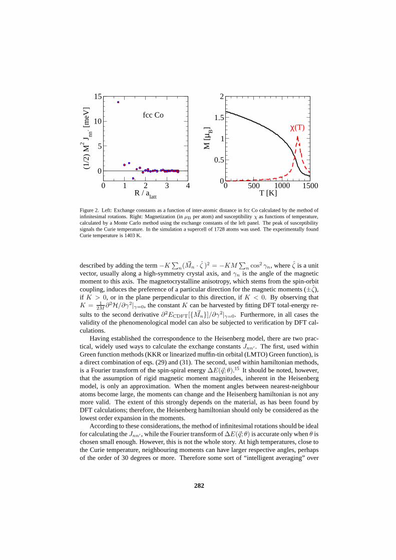
const. By computingE[{ ~Mn}] within constrained DFT, the RHS can be evaluated, andJnn′ can be found. Thus, the step from DFT to the Heisenberg model relies on acceptingthe equivalence of the DFT and Heisenberg-model excitationenergies. As an example wesee in fig. 2 the exchange constants of fcc Cobalt as a functionof distance.

Additional terms to the Heisenberg hamiltonian (30) can also be evaluated in a sim-ilar way. For instance, the magnetocrystalline anisotropyenergy is phenomenologically

281

0 1 2 3 4R / a

latt

0

5

10

15(1

/2)

M2 J

nn [m

eV]

0 500 1000 1500T [K]

0

0.5

1

1.5

2

M [

µ B] χ(T)

fcc Co

Figure 2. Left: Exchange constants as a function of inter-atomic distance in fcc Co calculated by the method ofinfinitesimal rotations. Right: Magnetization (inµB per atom) and susceptibilityχ as functions of temperature,calculated by a Monte Carlo method using the exchange constants of the left panel. The peak of susceptibilitysignals the Curie temperature. In the simulation a supercell of 1728 atoms was used. The experimentally foundCurie temperature is 1403 K.

described by adding the term−K∑

n( ~Mn · ζ )2 = −KM∑

n cos2 γn, whereζ is a unitvector, usually along a high-symmetry crystal axis, andγn is the angle of the magneticmoment to this axis. The magnetocrystalline anisotropy, which stems from the spin-orbitcoupling, induces the preference of a particular directionfor the magnetic moments (±ζ),if K > 0, or in the plane perpendicular to this direction, ifK < 0. By observing thatK = 1

2M ∂2H/∂γ2|γ=0, the constantK can be harvested by fitting DFT total-energy re-

sults to the second derivative∂2ECDFT[{ ~Mn}]/∂γ2|γ=0. Furthermore, in all cases the

validity of the phenomenological model can also be subjected to verification by DFT cal-culations.

Having established the correspondence to the Heisenberg model, there are two prac-tical, widely used ways to calculate the exchange constantsJnn′ . The first, used withinGreen function methods (KKR or linearized muffin-tin orbital (LMTO) Green function), isa direct combination of eqs. (29) and (31). The second, used within hamiltonian methods,is a Fourier transform of the spin-spiral energy∆E(~q; θ).15 It should be noted, however,that the assumption of rigid magnetic moment magnitudes, inherent in the Heisenbergmodel, is only an approximation. When the moment angles between nearest-neighbouratoms become large, the moments can change and the Heisenberg hamiltonian is not anymore valid. The extent of this strongly depends on the material, as has been found byDFT calculations; therefore, the Heisenberg hamiltonian should only be considered as thelowest order expansion in the moments.

According to these considerations, the method of infinitesimal rotations should be idealfor calculating theJnn′ , while the Fourier transform of∆E(~q; θ) is accurate only whenθ ischosen small enough. However, this is not the whole story. Athigh temperatures, close tothe Curie temperature, neighbouring moments can have larger respective angles, perhapsof the order of 30 degrees or more. Therefore some sort of “intelligent averaging” over

282

angles is called for, in order to increase the accuracy of results. The method of infinitesimalrotations can be systematically amended in this direction,as was proposed by Bruno,20

while for the Fourier-transform method larger anglesθ (perhaps of the order of 30 degrees)should be considered. We will return to this discussion in Section 8. We should alsomention that the formalism, as it is presented in the presentmanuscript, neglects the orbitalmoments and their interaction. Such effects can become important especially for rare earthsand actinides, which are, however, not well-described by local density functional theorydue to the strong electron correlations in these systems.

7 Solution of the Heisenberg Model

Having established the correspondence between DFT resultsand the Heisenberg hamilto-nian, and having identified the model parameters, a statistical-mechanical method is usedin order to solve the Heisenberg model, if one is interested in thermodynamic properties,or a dynamical method is used if one is interested in time-dependent properties. In theformer case, the Monte Carlo method, mean-field theory, and the random phase approx-imation (RPA) are most commonly used. For time-dependent properties we give a briefintroduction to Landau-Lifshitz spin dynamics.

7.1 Thermodynamic properties and the Curie temperature

The Monte Carlo method is a stochastic approach to the solution of the Heisenberg model(and of course to many other problems in physics). It is basedon a random walk in theconfiguration space of values of{ ~Mn}, but with an intelligently chosen probability fortransition from each state to the next. The random walk must fulfill two requirements: (i) itmust be ergodic, i.e., each point of the configuration space must be in principle accessibleduring the walk, and (ii) the transition probability between statesA andB, tA→B, mustobey the detailed balance condition, i.e.,P (A) tA→B = P (B) tB→A, whereP (X) =exp(−E(X)/kBT ) is the Boltzmann probability for appearance of stateX at temperatureT , with E(X) the energy of the state andkB the Boltzmann constant. As long as theserequirements are fulfilled,tA→B is to be chosen in a way that optimizes the efficiency ofthe method. The most simple and widely-used way is the Metropolis algorithm,21 in whichtA→B = P (B)/P (A) = exp[(E(A) − E(B))/kBT ] is taken forE(A) < E(B) andtA→B = 1 otherwise. For further reading on the Monte Carlo method we refer the readerto the book by Landau and Binder.22

Within the Monte Carlo method, a simulation supercell is considered, which containsmany atomic sites (e.g.,10 × 10 × 10 for simulating a three-dimensional cubic ferromag-netic lattice). At each site, a magnetic moment~Mn is placed, subject to interactionsJnn′

with the neighbours. Usually, periodic boundary conditions are taken in order to avoidspurious surface effects. During a Monte Carlo random walk,thermodynamic quantities(magnetization, susceptibility, etc.) are sampled and averaged over the number of steps. Inthis way it is possible, for instance, to locate the Curie temperatureTC of a ferromagnetic-paramagnetic phase transition by the drop of magnetizationor by the susceptibility peak.Since the simulation supercell is finite, the magnetizationdoes not fully disappear, and thesusceptibility peak overestimates somewhatTC. However, there are ways of correctingfor this deficiency, by increasing the supercell size and using scaling arguments.22 As an

283

Material TC(K) (exp) TC(K) (RPA) TC(K) (mean-field) Ref.Fe bcc 1044 950 1414 (a)Co fcc 1403 1311 1645 (a)Ni fcc 624 350 397 (a)

NiMnSb 730 900 1112 (b)CoMnSb 490 671 815 (b)Co2CrAl 334 270 280 (b)Co2MnSi 985 740 857 (b)

Table 1. Experimental and calculated Curie temperatures (in Kelvin, within the RPA) of various ferromagneticmaterials. Calculated values taken from: (a): Pajda et al,25 (b): Sasioglu et al.26

example we show in fig. 2 the temperature-dependent magnetization and susceptibility offcc Co calculated within the Monte Carlo method.

Mean-field theory is a physically transparent and computationally trivial way of esti-mating thermodynamic properties, however it lacks accuracy because it neglects fluctua-tions. As regards the Curie temperature, it is systematically overestimated by mean-fieldtheory (assuming applicability of the Heisenberg model). Given the exchange interactionsJnn′ the mean-field result forTC in a monoatomic crystal has the simple form

kB TC =1

3M2

∑

n′

Jnn′ . (32)

Another widely used method for estimating the Curie temperature is the random phaseapproximation. It yields results much improved with respect to mean-field theory with onlylittle increase of the computational burden. It is based on the Green function method for thequantum Heisenberg model, where a decoupling is introducedin the Green function equa-tion of motion, as proposed by Tyablikov fors = 1

2systems.23 Further refinements24, 25of

the RPA for higher-spin systems allow the transition to the classical limit by takings→ ∞.The Curie temperature in a monoatomic lattice is then given by

1

kB TC

=3

2

1

N

∑

~q

1

E(~q)(33)

whereE(~q) is the magnon (or spin-spiral) energy, calculated by a Fourier transform ofJnn′ or directly by constrained DFT, andN the number of atoms in the system. For multi-sublattice systems, a modified version of RPA can be used.26

7.2 Time-dependent magnetic properties and Landau-Lifshitz spin dynamics

In case that one is interested in the time dependence of the magnetic moments under the in-fluence, e.g., of an external field pulse, the method of magnetization dynamics can be used.The classical equations of motion associated with this method are the Landau-Lifshitzequations for the moments{ ~Mn},

d ~Mn

dt= ~Heff

n × ~Mn, (34)

~Heffn =

∑

n′

Jnn′~Mn′ + ~Hext. (35)

284

These are first-order equations in time which describe the precession of the magnetic mo-ment due to external fields (different than an electric dipole, which will rotate towardsthe direction of an electric field, the magnetic dipole is essentially an angular momentumand therefore will precess around a magnetic field). The effective field defined in eq. (35)comprises the exchange interaction with the neighbours andan externally applied mag-netic field. However, other terms can be included in~Heff

n , such as the magnetocrystallineanisotropy or the magnetic field created by the very moments of the material itself—thelatter becomes most important in large ferromagnetic systems, and we discuss in the nextsubsection.

As is obvious by taking the dot product of eq. (34) with~Mn, ~Mn · d ~Mn/dt = 0, i.e.,the Landau-Lifshitz equations conserve the magnitude of the moments. They also conservethe total energy. However, dissipation effects that lead todamping of the precession can betaken into account by an additional phenomenological term of the formλ( ~Heff

n × ~Mn) ×~Mn, where a parameterλ describes the damping strength. Temperature effects can also be

simulated by additional phenomenological terms of stochastic forces, through an approachsimilar to Langevin molecular dynamics.27

We should note here the existence of a formalism for fully ab-initio spin dynamics,i.e., without the assumption of a Heisenberg model.28 (From this formalism the Landau-Lifshitz equations follow as a limiting case.) However, this approach is computationallyheavy, as it requires self-consistent density functional calculations at each time step of thesystem evolution.

7.3 Dipolar field calculation and related multiscale modelling

We now discuss the effect of the dipole-dipole interaction on the magnetic configuration.By this we mean the interaction of each magnetic dipole (here, atomic magnetic moment)with the magnetic field created by all other dipoles in the system. It is well-known thatthe this type of interaction between two moments~Mn and ~Mn′ , connected by a vector~Rnn′ = ~Rn − ~Rn′ , has the form

Edip(~R) =3 ( ~Mn · ~Rnn′)( ~Mn′ · ~Rnn′) − ( ~Mn · ~Mn′)R2

nn′

R5nn′

(36)

Equivalently, each moment feels a magnetic field, thedipolar field ~Hdipn , to be included in

~Heffn in the Landau-Lifshitz equation, of the form

~Hdipn =

∑

n′ 6=n

3 ~Rnn′( ~Mn′ · ~Rnn′) − ~Mn′ R2nn′

R5nn′

(37)

Compared to the nearest-neighbour exchange interactionsJnn′ , the interaction betweentwo dipoles is weak, but the complication is that the summation (37) cannot be restrictedto a few neighbours only, as it falls off relatively slowly with distance (∼ 1/R3

nn′). Espe-cially in three-dimensional systems the sum is guaranteed to converge only by finite-sizeeffects of the sample, i.e., it becomes a meso- or macroscopic property and the sampleboundaries become important.a ~Hdip

n is evidently time-consuming to calculate; particu-larly a brute-force calculation would be impossible for large systems. There are, however,

aIn large ferromagnetic systems the dipolar field cannot be neglected, as it is responsible for the emergence ofmagnetic domains.

285

special techniques that allow for a fast, approximate calculation of ~Hdipn . This is even more

crucial for spin dynamics, as~Hdipn depends on the moments configuration and has to be

calculated anew at each time step.One such technique is thefast multipole method, originally introduced to treat the prob-

lem of Coulombic interactions.29 The central idea is to divide space in regions of differentsizes, and treat the collective field from each region by a multipole expansion up to a cer-tain order. The higher the order, the more accurate and expensive the calculation. Given acertain expansion order, regions that are far away from the point of field-evaluation can belarge, while regions that are close have to be smaller to maintain accuracy (the criterion ofregion size is the opening angleD/R, withD the diameter of the region andR its distancefrom the point of field-evaluation). An essential ingredient of the fast multipole methodis the efficient derivation of multipoles of a large region from the multipoles of its sub-regions. This derivation requires the calculation of multipole expansion and translationcoefficients, which, however, depend only on the geometry and for magnetic systems haveto be evaluated only once (as the magnetic moments are not moving).

A fast evaluation of the dipolar field allows for multiscale simulations in magneto-statics30 or magnetization dynamics, also in a sense that we have not discussed up to thispoint. In such simulations, the transition from the large (mesoscopic or even macroscopic)scale to the atomic scale is done in a seamless way. The idea isto treat the magneti-zation as a continuous field by a coarse grained approach in regions where it is relativelysmooth, whereas to gradually refine the mesh, even up to the atomic limit, in regions wherethe spatial fluctuations become more violent (e.g. magneticvortex cores, Bloch points,monoatomic surface step edges, ferromagnet-antiferromagnet interfaces, etc.). In the con-tinuum limit, however, the Landau-Lifshitz equations (34)must be rewritten in terms of acontinuous magnetization~M(~r) and thespin stiffnessA:

d ~M(~r)

dt= ~Heff(~r) × ~M(~r) (38)

~Heff(~r) =2

M2s

A∇2 ~M(~r). (39)

Ms = | ~M(~r)| is the absolute value of the continuum magnetization (also called satu-ration magnetization in ferromagnetic samples). The termA∇2 ~M(~r) results from tak-ing

∑

n′ Jnn′~Mn′ to the continuum limit; the spin stiffness is given (in an example of a

monoatomic crystal with atomic momentM and primitive cell volumeVc) in terms of theexchange constants asA = (1/4Vc)M

2∑

n J0nR2n, with Rn the distance of atomn from

the origin.

8 Back-Coupling to the Electronic Structure

So far we have discussed how the transition from the DFT to theHeisenberg model isachieved by fitting the Heisenberg model parameters to DFT total energies at and close tothe ground state. However, at higher temperature (close to the Curie temperature, that canbe of the order of 1000 K) the local electronic structure can change. Several mechanismscan contribute to this: lattice vibrations, single-electron excitations, collective electronic

286

excitations such as magnons, structural phase transitions(such as the hcp to fcc transi-tion of Cobalt above 700 K) etc. As a consequence, the pair exchange parametersJnn′

calculated from the low-temperature electronic structurecould be significantly altered.Perhaps the most serious effect can be caused by the non-collinear magnetic configura-

tions at high temperature, in which the angle between first-neighbouring moments can beof the order of30◦. At such high angles, and depending on the system, the parametrizationof the total energy with respect to the Heisenberg model can be insufficient—recall that, inprinciple, the Heisenberg hamiltonian is justified as the lowest-order term in an expansionwith respect to the angle. An often encountered consequenceof an altered local electronicstructure is a change of the atomic moments. Furthermore, asthis angle is not static, butfluctuating in time, it is no use to simply perform static non-collinear calculations at thisangle and derive theJnn′ by small deviations. We are thus faced with the problem of aback-coupling of the high-temperature state to the electronic structure; i.e., of approximat-ing the local electronic properties in the presence of thermal fluctuations.

Two solutions are frequently used to this problem. The first is to go beyond the Heisen-berg model and perform a more thorough parametrization of the energy as a function of themoments, including also possible changes in the magnitude of the moments. This methodhas been applied, e.g., by Uhl and Kubler.31 The disadvantage is that it can be computa-tionally expensive, both due to the number of self-consistent constrained-DFT calculationsrequired for a parametrization of the multi-dimensional space{ ~Mn}, and because of themore involved Monte Carlo calculations where the change of the moments magnitude hasto be accounted for. There are, however, reasonable approximations that can reduce thenecessary number of parameters, while the Curie temperature can be found within a mod-ified mean-field theory.31

The second solution is to assume that the Heisenberg model isstill adequate to describethe phase transition, but with “renormalized” parameters,chosen such that the change ofthe local electronic structure is taken into account by an averaging over angles. This solu-tion is intuitive but certainly not rigorous. It is, however, simple to include within Greenfunction electronic structure methods, by assuming an analogy of the high-temperaturestate with a spin-glass state and employing the coherent potential approximation (CPA).Spin-glass systems are characterized bydisordered local moment(DLM) states, consistingof two different magnetic “species” that correspond, say, to the magnetic moment pointing“up” (A) or “down” (B). These are encountered in a random manner with a probability1 − x andx, respectively: the DLM state is of the formA1−xBx. Forx = 0 we recoverthe ferromagnetic state, while forx = 0.5 we have complete magnetic disorder. (Note thata DLM state is different than the antiferromagnetic state, in which the speciesA andB arewell-ordered in two sublattices.) Under the assumption of an analogy of high-temperaturestates in ferromagnets to DLM systems, the ferromagnet at the Curie temperature is ap-proximated by the alloyA0.5B0.5.

The CPA is a method for the description of chemical disorder in alloys, and can be ap-plied here to the magnetic type of alloyA0.5B0.5. Within the CPA, the Green functionGand scattering matrixt of an effective average medium are sought, such that the additionalscattering of atomsA andB in this medium vanishes on the average. We skip the deriva-tion, which can be found in many textbooks,32, 33 and give only the final CPA condition

287

that has to be fulfilled:

t−1

= (1 − x) t−1A + x t−1

B + (t−1

− t−1A )(t

−1− G)−1(t

−1− t−1

B ), (40)

G = g (1 − tg)−1 (41)

with g the free-space structural Green function in the KKR formalism.16 Expression (41)is the Dyson equation for the Green function of the average medium, which depends on theaverage-medium scattering matrixt. The latter is determined by Eq. (40), which containst

also on the right-hand side (explicitly and also throughG), and is solved self-consistentlyby iteration. At the end, the Green functions of speciesA andB are projected out from theaverage medium Green function again via the Dyson equation

GA,B = G(

1 − (tA,B − t) G)−1

(42)

and used for the calculation of the electronic structure of the two atomic species.Given the CPA Green function for theA0.5B0.5 DLM state, the method of infinitesimal

rotations can be employed to obtain the pair exchange constants. Assuming that the DLMstate represents the magnetic structure at the Curie temperature, the exchange constantsobtained by this method should be more appropriate to use in the Heisenberg hamiltonianclose toTC than the ones obtained from the ground state. However, this is not guaranteed,especially in view of the fact that the CPA neglects the short-range magnetic order that ispresent even atTC.

9 Concluding Remarks

The Multiscale Programme discussed here is widely used today, however, the matter issurely not closed. Mainly two types of difficulties are present and are the subject of cur-rent research. First, density functional theory within thelocal spin density or generalizedgradient approximation is not able to describe the ground state properties of every mate-rial. When electron correlations (on-site electron-electron repulsion and temporal electrondensity fluctuations) become particularly strong, these approximations fail. Characteristicof such problems aref -electron systems, transition metal oxides or molecular magnets.Improved concepts exist and are applied, such as the LSDA+U or dynamical mean-fieldtheory, however, at the moment these methods rely on parameters that cannot always befound without a fit to experiment.

Second, the excited state properties are also not always accessible to density functionaltheory. The adiabatic hypothesis, together with constrained DFT, work up to a point, buteffects as the magnon lifetime or frequency-dependent interactions are neglected. Currentwork in this direction is done within approximations as theGW or time-dependent DFT,with promising results. These methods are, however, still computationally very expensive,and the extent of improvement that they can offer to the calculation of thermodynamicalproperties remains unexplored.

Acknowledgments

I am grateful to D. Bauer, S. Blugel, P.H. Dederichs, R. Hertel, M. Lezaic, S. Lounis, andL.M. Sandratskii for illuminating discussions on the subjects presented in this work.

288

References

1. P. Hohenberg and W. Kohn Phys. Rev.136, B864 (1964).2. W. Kohn and L. J. Sham Phys. Rev.140, A1133 (1965).3. U. von Barth and L. Hedin, J. Phys. C: Solid State Phys.5, 1629 (1972).4. V.L. Moruzzi, J.F. Janak, and A.R. Williams,Calculated electronic properties of met-

als (Pergamon, New York 1978).5. D.M. Ceperley and B.J. Alder, Phys. Rev. Lett.45, 566 (1980).6. S.H. Vosko, L. Wilk, and M. Nusair, Can. J. Phys.58, 1200 (1980).7. See, for example, J.P. Perdew, K. Burke, and Y. Wang, Phys.Rev. B 54, 16533

(1996); J.P. Perdew, K. Burke, and M. Ernzerhof, Phys. Rev. Lett. 77, 3865 (1996).8. V.I. Anisimov, F. Aryasetiawan, and A.I. Lichtenstein J.Phys.: Condens. Matter9,

767 (1997).9. P.H. Dederichs, R. Zeller, H. Akai, and H. Ebert, J. Magn. Magn. Matter100, 241

(1991).10. P.H. Dederichs, S. Blugel, R. Zeller, and H. Akai, Phys.Rev. Lett.53, 002512 (1984).11. A. Oswald, R. Zeller, and P. H. Dederichs, J. Magn. Magn. Mater. 54-57, 1247

(1986); N. Stefanou and N. Papanikolaou, J. Phys.: Condens.Matter5, 5663 (1993).12. A.R. Mackintosh and O.K. Andersen,The electronic structure of transition metals, in:

Electrons at the Fermi surface, Ed. by M. Springfold (Cambridge University Press,Cambridge, 1980); M. Weinert, R. E. Watson, and J. W. Davenport, Phys. Rev. B32,2115 (1985); V. Heine, Solid State Phys. 35, 1 (1980); M. Methfessel and J. Kubler,J. Phys. F 12, 141 (1982).

13. A. Oswald, R. Zeller, P.J. Braspenning, and P.H. Dederichs, J. Phys. F15, 193 (1985).14. L.M. Sandratskii, Phys. Stat. Sol. (b) 135, 167 (1986).15. S. V. Halilov, H. Eschrig, A. Y. Perlov, and P. M. Oppeneer, Phys. Rev. B58, 293

(1998).16. P. Mavropoulos and N. Papanikolaou,The Korringa-Kohn-Rostoker (KKR)

Green Function Method I. Electronic Structure of Periodic Systems, in Com-putational Nanoscience: Do It Yourself!, eds. J. Grotendorst, S. Blugel, andD. Marx, Winterschule, 14.-22. Februar 2006, (Forschungszentrum Julich 2006);http://www.fz-juelich.de/nic-series/volume31/volume31.html

17. P.H. Dederichs, S. Lounis, and R. Zeller,The Korringa-Kohn-Rostoker (KKR)Green Function Method II. Impurities and Clusters in the Bulk and on Surfaces, inComputational Nanoscience: Do It Yourself!, eds. J. Grotendorst, S. Blugel, andD. Marx, Winterschule, 14.-22. Februar 2006, (Forschungszentrum Julich 2006);http://www.fz-juelich.de/nic-series/volume31/volume31.html

18. S. Lounis, Ph. Mavropoulos, P. H. Dederichs, and S. Blugel Phys. Rev. B72, 224437(2005).

19. A.I. Liechtenstein, M.I. Katsnelson, V.P. Antropov, and V.A. Gubanov,J. Magn. Magn. Mater.6765 (1987).

20. P. Bruno, Phys. Rev. Lett.90, 087205 (2003).21. N. Metropolis, A. Rosenbluth, M. Rosenbluth, A. Teller,and E. Teller, J. Chem. Phys.

21, 1087 (1953).22. D.P. Landau and K. Binder,A Guide to Monte Carlo Simulations in Statistical

Physics, Cambridge University Press (2000).

289

23. S.V. Tyablikov,Methods of Quantum Theory of Magnetism(Plenum Press, New York,1967).

24. H. B. Callen, Phys. Rev.130, 890 (1963).25. M. Pajda, J. Kudrnovsky, I. Turek, V. Drchal, and P. Bruno, Phys. Rev. B64, 174402

(2001).26. E. Sasioglu, L. M. Sandratskii, P. Bruno, and I. Galanakis, Phys. Rev. B72, 184415

(2005).27. See, for example, V.P. Antropov, S.V. Tretyakov, and B.N. Harmon, J. Appl. Phys.

81, 3961 (1997).28. V. P. Antropov, M. I. Katsnelson, B. N. Harmon, M. van Schilfgaarde, and D. Kusne-

zov, Phys. Rev. B54, 1019 (1996).29. L. Greengard and V. Rokhlin, J. Comput. Phys. 73, 325 (1987).30. Thomas Jourdan, Alain Marty, and Frederic Lancon, Phys.Rev. B77, 224428 (2008).

A. Desimone, R.V. Kohn, S. Muller, and F. Otto, Multiscale Modeling and Simulation1, 57 (2003).

31. M. Uhl and J. Kubler, Phys. Rev. Lett.77, 334 (1996).32. J. Kubler,Theory of Itinerant Electron Magnetism, Oxford University Press, 2000.33. A. Gonis,Theoretical Materials Science, Materials Science Society, 2000.

290