Yao, Li (2006) Magnetic field modelling of machine and...
269
Yao, Li (2006) Magnetic field modelling of machine and multiple machine systems using dynamic reluctance mesh modelling. PhD thesis, University of Nottingham. Access from the University of Nottingham repository: http://eprints.nottingham.ac.uk/10224/1/LiYAO-Final_Binded_PhD_Thesis.pdf Copyright and reuse: The Nottingham ePrints service makes this work by researchers of the University of Nottingham available open access under the following conditions. This article is made available under the University of Nottingham End User licence and may be reused according to the conditions of the licence. For more details see: http://eprints.nottingham.ac.uk/end_user_agreement.pdf For more information, please contact [email protected]
Transcript of Yao, Li (2006) Magnetic field modelling of machine and...

Yao, Li (2006) Magnetic field modelling of machine and multiple machine systems using dynamic reluctance mesh modelling. PhD thesis, University of Nottingham.
Access from the University of Nottingham repository: http://eprints.nottingham.ac.uk/10224/1/LiYAO-Final_Binded_PhD_Thesis.pdf
Copyright and reuse:
The Nottingham ePrints service makes this work by researchers of the University of Nottingham available open access under the following conditions.
This article is made available under the University of Nottingham End User licence and may be reused according to the conditions of the licence. For more details see: http://eprints.nottingham.ac.uk/end_user_agreement.pdf
For more information, please contact [email protected]

MAGNETIC FIELD MODELLING OF
MACHINE AND MULTIPLE MACHINE SYSTEMS USING DYNAMIC RELUCTANCE
MESH MODELLING
By Li Yao
BEng (Honours), Msc (Engineering)
Thesis submitted to the University of Nottingham for the degree of Doctor of Philosophy
May 2006

Abstract
i
ABSTRACT
This thesis concerns the modified and improved, time-stepping, dynamic
reluctance mesh (DRM) modelling technique for machines and its application
to multiple machine systems with their control algorithms. Improvements are
suggested which enable the stable solution of the resulting complex non-linear
equations. The concept of finite element (FE) derived, overlap-curves has been
introduced to facilitate the evaluation of the air-gap reluctances linking the
teeth on the rotor to those on the stator providing good model accuracy and
efficient computation. Motivated industrially, the aim of the work is to develop
a fast and effective simulation tool principally for evaluating salient pole
generator system designs including the generator, exciter and the automatic
voltage regulator (AVR). The objective is to provide a modelling system
capable of examining the detail of machine operation including saturation of
main and leakage flux paths, slotting and space harmonics of the windings.
Solutions are obtained in a sufficiently short computational time to facilitate
efficient iterative design procedures in an industrial design office.
The DRM modelling technique for electrical machines has been shown in this
thesis to be a fast and efficient tool for electrical machine simulation. Predicted
results for specific machine and system designs have been compared with FE
solutions and with experimental results showing, that for engineering purposes,
the technique yields excellent accuracy.
The DRM method has a great advantage in multiple machine simulations. This
is because magnetic field calculations are limited to evaluating only the most
important information so saving computation time. A brushless generating
system including the excitation system and control scheme has been modelled.
Additionally a cascaded, doubly fed induction generator for wind generator
applications has also been modelled. These different applications for the

Abstract
ii
dynamic reluctance mesh method have proved that this approach yields an
excellent machine and machine-system evaluation and design tool.

Acknowledgements
iii
ACKNOWLEDGEMENTS
Firstly, I would like to express my sincere gratitude to my supervisors, Dr.
Keith Bradley and Professor Phil Sewell for their invaluable assistance and
guidance with my research study during the past three and a half years at the
University of Nottingham. Also, I would like to express my appreciation to
Newage AVK SEG UK for the financial support and their sincere help with the
experimental data.
I would like to thank all my colleagues in the PEMC group, at the University of
Nottingham, for their encouragement, support and friendship throughout the
years. In particularly to Ungku Anisa Ungku Amirulddin and Chris Gerada,
with whom I had very helpful conversations related to my research. Thanks
also go to my friends and housemates in Nottingham over these years for their
help and the fun moments that we shared.
Finally, I would like to express my deepest gratitude to my parents, family who
have relentlessly supported me in every possible way throughout my study in
the UK, and for their never ending love and encouragement.

List of Symbols
iv
LIST OF SYMBOLS
A area of airgap reluctance element (m2)
B flux density (Tesla or Wb/m2)
b , pb width for salient pole shoes and poles (m)
sc , pc distance between parallel salient pole shoes and poles (m)
D machine windage
i
a
ddeφ
,i
b
ddeφ
,i
c
ddeφ
terms representing the change of the emf induced in
phase A , B orC due to a change of flux in tooth i
iE energy stored in each air gap element (J)
afE , bfE , cfE generated emf of stator three phase (V)
dE′ , qE′ added d and q axis voltages represent transient voltage in
the generator (V)
dE ′′ , qE ′′ added d and q axis voltages represent sub-transient voltage
in generator (V)
( )xF matrix of state equations solved by the DRM software
kF mmf source (A)
lF mmf source value for salient rotor windings (A)
if mmf at node I (A)
1f , 2f , 3f , 4f frequencies for side 1,2,3 and 4 in cascaded doubly fed
induction machine system (Hz)
mf rotor rotating mechanical frequency (Hz)
H flux field intensity (A/m)

List of Symbols
v
sh , ph height for salient pole shoes and poles (m)
cba iii ,, three phase current (A)
fi synchronous machine field current (A)
sI leakage current for diode (A)
J machine inertia (Kg m2)
Jr
current density (A/m2)
J jacobian matrix
gK carter’s factor used in extended air gap length calculations
ok carter’s factor referenced from carter’s curve
gl air gap length (m)
gl′ extended air gap length (m)
lqld LL , d and q axis leakage inductance (H)
mdL , mqL d-axis and q-axis magnetization inductance (H)
rL , rλ rotor inductance and flux linkage for synchronous
machine (H, Wb)
sL , pL length for salient pole shoes and poles (m)
lfdL field winding leakage inductance in salient pole
synchronous machine (H)
lkdL′ , 1lkqL′ referred damper winding d-axis and q-axis leakage
inductance in salient pole synchronous machine (H)
nodeN number of node in the reluctance mesh in DRM
barN number of damper bars in the induction machine
pn number of parallel paths in stator winding

List of Symbols
vi
sN number of stator slots
P Park’s transformation matrix
p Newton step in Newton-Raphson algrithm
Ap , Bp number of pole pairs in cascaded doubly fed induction
machine system
mechP mechanical power of the shaft (J)
electricalconverterP power flowing out of the converter side machine’s stator
(J)
electricalgeneratedP power flowing out of the grid side machine’s stator (J)
lossP power loss (J)
cba RRR ,, phase resistance of A, B and C (Ω )
fR synchronous machine field resistance (Ω )
sqsd RR , salient pole synchronous machine stator d and q axis
resistance (Ω )
fdR′ referred salient pole synchronous machine field resistance
(Ω )
kdR′ , 1kqR′ referred damper winding d-axis and q-axis resistance in
salient pole machine (Ω )
S number of stator teeth
eT electrical torque in the machine (N.m)
loadT mechanical load torque in the machine (N.m)
cT turns per coil for stator
phT turns per phase
V volume (m3)

List of Symbols
vii
CBA vvv ,, three phase voltage (Volts)
fv synchronous machine field voltage (Volts)
ow slot opening (m)
dlw ,, width, length and depth of the reluctance elements (m)
slw , plw effective width for leakage reluctance between pole shoes
and poles in a salient pole rotor (m)
widtheffectivew air gap reluctance effective width when taking fringing
into account (m)
x vector of state variables
oldx , newx vector of state variables at initial value and solving value
fron Newton-Raphson method
saX , sbX , scX synchronous reactance for synchronous machine (Ω )
aX , bX , cX magnetizing reactance for synchronous machine (Ω )
lX leakage reactance for synchronous machine (Ω )
dX , qX direct- and quadrature- axis synchronous reactances for
salient pole machine (Ω )
lsX stator leakage reactance (Ω )
mdX , mqX magnetizing reactance for d and q axis for salient pole
synchronous machine (Ω )
sy slot pitch (m)
pλ line searched Newton step
0µ permeability of vacuum (H/m)
rµ relative permeability
rµµµ 0= permeability of an element (H/m)

List of Symbols
viii
ijα factor for thi stator or rotor teeth determines the presence
or absence of the thj phase current in the slot
rω Shaft speed (rad/sec)
φ flux (wb)
λ flux linkage (Wb)
mechθ mechanical angle of the shaft (rad)
mφ main flux between the stator and rotor in a salient pole
generator (Wb)
1φ , 2φ leakage flux between salient pole shoes (Wb)
3φ , 4φ leakage flux between salient poles (Wb)
ℜ reluctance (m/H)
δ load angle (deg)

List of Figures
ix
LIST OF FIGURES Figure 1.2.1 Typical topology structure of a power station 3
Figure 1.2.2 Appearance of a typical small industrial brushless generating
system 6
Figure 1.2.3 Internal structure of a typical small brushless generating system
6
Figure 2.2.1 Reluctance in magnetic circuit 16
Figure 2.2.2 Reluctances in DRM reluctance mesh 17
Figure 2.2.3 Simplified B-H curve for ferromagnetic material Losil 800 19
Figure 2.2.4 Mmf source placing by DRM method for electric machine 20
Figure 2.2.5 Reluctances connected with mmf source in DRM reluctance mesh
21
Figure 2.2.6 A typical induction machine reluctance mesh discretisation 21
Figure. 2.2.7 Induction machine stator and rotor dimensions 23
Figure 2.2.8 A simple air gap magnetic circuit includes air gap 23
Figure 2.2.9 Air gap in a simple magnetic circuit 24
Figure 2.2.10 Air gap reluctances in electrical machine magnetic circuit 25
Figure 2.2.11 Dynamic creations of air gap reluctances in DRM method 26
Figure 2.2.12 Skew model of cage rotor 28
Figure 2.2.13 Trapezoidal rotor tip elements 28
Figure 2.2.14 Trapezoidal air gap elements in DRM modelling 29
Figure 2.2.15 Torque ripple comparison for the result come from induction
machine direct on line start no load condition simulation, with air gap modelled
by rectangular and trapezoidal shape elements 30
Figure 2.2.16 Number of iteration comparison for the results come from
induction machine direct on line start no load condition simulation, with air
gap modelled by rectangular and trapezoidal shape elements 30
Figure 2.3.1 Conservation of rate of change of flux in one node 32
Figure 2.3.2 Coupling of a single turn electrical network with the reluctance
mesh 32
Figure 2.3.3 Coupling of electrical network and magnetic circuit in a cage rotor
34

List of Figures
x
Figure 2.4.1 solutions of two nonlinear equations. The grey regions are the
positive regions for the function f and the dashed lines divide the plane into
positive and negative regions for the system 38
Figure 2.4.2 Newton method in one dimensional to find the next predicted
value 39
Figure 2.4.3 Initial guess is not close enough to the solution and
nonconvergence situation happened in Newton-Raphson method 40
Figure 2.4.4 Newton-Raphson method encounters a local extreme where high
order terms are important and cannot be neglected 40
Figure 2.4.5 Schematic diagram shown the relationship between memory usage
and the number of linear solver iteration with respect to threshold 43
Figure 2.4.6 DRM program flow chart 47
Figure 3.2.1 Air gap modelling in DRM: method 1 52
Figure 3.2.2 Air gap elements calculated by method 1 52
Figure 3.2.3 Different stator and rotor overlap conditions in a skewed rotor
section 53
Figure 3.2.4 Air Gap reluctance effective width curves for a specific type of
induction machine with different skew angles with method 1 54
Figure 3.2.5 Air gap surface opening 55
Figure 3.2.6 Overlap curves model for induction machine for method 3 58
Figure 3.2.7 Air gap overlap curves for a specific geometry of induction
machine with different methods 59
Figure 3.2.8 Sub skew sections for effective air gap reluctance calculation in a
skewed rotor induction machine 61
Figure 3.2.9 Comparison of speed curve for a skewed rotor induction machine,
simulated with one skew section 63
Figure 3.2.10 Comparison of speed curve for a skewed rotor, simulated with
three skew section 64
Figure 3.2.11 Speed curve comparison with a non-skewed rotor induction
machine 65
Figure 3.4.1 The adjusting of time step and the changing of system error with
respect to the number of restart times in a synchronous machine generating
system 68
Figure 3.4.2 Flow chart of line search backtrack algorithm 74

List of Figures
xi
Figure 3.4.3 Solving process of a globally convergent Newton-Raphson solver
75
Figure 3.4.4 Number of NR iteration for globally convergent nonlinear solver
vs. time step 76
Figure 3.5.1 Air gap reluctances between stator and rotor teeth 78
Figure 3.5.2 Slot leakage flux pattern in parallel slots, accommodating one
rectangular conductor 78
Figure 3.5.3 Semi-closed slot profiles 79
Figure 3.5.4 Schematic plot of slot leakage reluctance calculation 80
Figure 3.5.5 Round slot profiles 81
Figure 3.5.6 Modified dynamic reluctance mesh for induction machine which
accounts for slot leakage flux 82
Figure 3.5.7 Induction machine direct on line start speed curve, with and
without slot leakage reluctance modelled, in comparison to FEM results 83
Figure 4.2.1 Equivalent circuit of cylindrical synchronous generator 88
Figure 4.2.2 Phase diagram of cylindrical synchronous generator in steady state
under excited 89
Figure 4.2.3 Phase diagram for salient-pole synchronous generator 91
Figure 4.2.4 Two pole, three phase, salient pole synchronous machine windings
arrangements 92
Figure 4.2.5 Complete synchronous machine d- and q- axis equivalent circuit
93
Figure 4.3.1 Solution mesh of the salient-pole synchronous machine in a
specific time step @100ms 98
Figure4.3.2 Electrical circuit connection model of a type of salient-pole
synchronous generator simulated in FEM software 99
Figure 4.3.3 Flux function distribution in a salient-pole synchronous machine
calculated by FEM software, results taken @100ms 100
Figure 4.3.4 Field current comparison between FEM and DRM calculations
101
Figure 4.3.5 Stator current comparison between FEM and DRM results 102
Figure 4.3.6 Torque and air - gap flux density (magnitude) of this type of
machine simulated by FEM software 103

List of Figures
xii
Figure 4.4.1 Flux distribution for a salient pole generator, rated field voltage
excited and stator terminals are open circuited 106
Figure 4.4.2 Virtual rotor teeth on the surface of salient-pole rotor 107
Figure 4.4.3 Overlap curves for salient-pole synchronous machines 108
Figure 4.4.4 Angular displacement of salient pole synchronous machine 108
Figure 4.4.5 Reluctance mesh shows the leakage air-gap reluctance and inter-
pole reluctances in salient-pole machine 110
Figure 4.4.6 Parallel leakage flux path between each pair of pole shoes 102
Figure.4.4.7 Whole air gap reluctance mesh for salient pole generator,
including leakage and inter-pole reluctances 113
Figure4.4.8 A typical complete salient pole rotor reluctance mesh 115
Figure 4.4.9 reluctance mesh topology for modelling of damper bars which has
‘fake’ internal flux loop 117
Figure 4.4.10 Virtual Damper Bars and mmfs 118
Figure 4.4.11 Real damper bar construction between two poles 119
Figure 4.4.12 Virtual damper bar modelling between two salient-poles 119
Figure 4.4.13 Proposed complete salient pole rotor reluctance mesh 120
Figure 4.5.1 Schematic drawing of electrical connection for the generator to be
simulated 123
Figure 4.5.2 Experimental result of open circuit test and short circuit test 124
Figure 4.5.3 Open circuit result comparison for DRM and experiment data 126
Figure 4.5.4 Short circuit test result comparison between DRM and experiment
127
Figure 4.5.5 Sudden short circuit test, stator line-to-line voltage 128
Figure 4.5.6 Sudden short circuit test stator phase current 129
Figure 4.5.7 Sudden short circuit test, stator phase B current 130
Figure 4.5.8 Sudden short circuit test, stator phase C current 130
Figure 4.5.9 Sudden short circuit test, generator field current 131
Figure 4.5.10 Sudden short circuit test, damper bar current 132
Figure 4.5.11 Sudden short circuit test, max B in stator tooth tip reluctances
133
Figure 4.5.12 Sudden short circuit test, number of NR iterations 133
Figure 4.5.13 Adjacent Damper bar currents 134

List of Figures
xiii
Figure 4.5.14 Field current comparison for generators with and without damper
bars, at a rated load running condition 135
Figure 5.1.1 Conventional excitation of generator systems 138
Figure 5.1.2 Static excitation of generator systems 139
Figure 5.1.3 Brushless excitation of generator systems 140
Figure 5.1.4 Brushless excitation with pilot exciter of generator system 140
Figure 5.2.1 Exciter geometry, with field winding staying on the stator and
armature winding on the rotor 142
Figure 5.2.2 Sections of Exciter Reluctance Mesh Model 143
Figure 5.2.3 Exciter Air Gap Reluctance Curves 144
Figure 5.2.4 Exciter current waveforms in a numerical simulated open circuit
condition 147
Figure 5.3.1 Six diodes full Wave three-phase bridge rectifier 148
Figure 5.3.2 Ideal diode and its circuit symbol 149
Figure 5.3.3 Practical diode iv − Characteristic 150
Figure 5.3.4 Diode model in the rotating rectifier model in the DRM Modelling
151
Figure 5.4.1 Schematic generating system diagram 151
Figure 5.4.2 Electrical circuit diagram of generating system 152
Figure 5.4.3 Rearranged electrical circuit of generating system 152
Figure 5.5.1 Experimental result for exciter+rectifiers+main generator 157
Figure 5.5.2 DRM simulation results in comparison to modified experimental
results for open circuit testing 159
Figure 5.6.1 General functional block diagram for generator excitation control
system 161
Figure 5.6.2 IEEE std. 421.5 Type AC5A- simplified rotating rectifier
excitation system representations 161
Figure 5.6.3 The practical excitation system model for the generating system in
the thesis 162
Figure 5.6.4 Excitation control model used in the simulation in this thesis 163
Figure 5.6.5 Transfer function model of excitation control system described in
the thesis 163
Figure 5.6.6 First order system transfer function 163
Figure 5.6.6 Deriving the field time constant of exciter 164

List of Figures
xiv
Figure 5.6.7 Deriving the field time constant of main generator 165
Figure 5.6.8 Simulated voltage sensing in DRM simulation 166
Figure 5.6.9 Digital PID controller used in this thesis 167
Figure 5.7.1 Generated stator per phase voltage for the complete generating
system 169
Figure 5.7.2 Error between reference voltage value and feedback voltage value
170
Figure 5.7.3 AVR controller output value 170
Figure 5.7.4 Generated stator per phase voltage for the complete generating
system during a voltage dip 171
Figure 5.7.5 Error between reference voltage value and feedback value during
a voltage dip 171
Figure 5.7.6 AVR controller output value during a voltage dip 172
Figure 6.1.1 Fixed speed wind generating system 175
Figure 6.1.2 Variable speed wind generating system with stator side converter
176
Figure 6.1.3 Variable speed wind generating system with rotor side converter
176
Figure 6.2.1 Cascaded doubly-fed induction machine (CDFM) 178
Figure 6.2.2 Frequency relationship in series connected cascaded doubly fed
induction machines 179
Figure 6.3.1 Electrical and mechanical connection diagram of cascaded
machine system 181
Figure 6.3.2 Electrical connection loop between the rotors in cascaded
induction machines 182
Figure 6.4.1 Frequency relations in sub-synchronous speed - 550 rpm for
CDFM 185
Figure 6.4.2 Converter side (side 4) induction machine stator current waveform
186
Figure 6.4.3 Cascaded machine rotor phase A current (side 2 & 3) 187
Figure 6.4.4 Grid side stator current waveform (side 1) 187
Figure 6.4.5 Power flow condition in sub-synchronous speed 188
Figure 6.4.6 Power flow relationship between terminals in sub-synchronous
speed 189

List of Figures
xv
Figure 6.4.7 Frequency relations in super-synchronous speed - 950 rpm for
CDFM 190
Figure 6.4.8 Converter side (side 4) induction machine stator current waveform
191
Figure 6.4.9 Rotor current waveform (side 2 & 3) 191
Figure 6.4.10 Grid side (side 1) induction machine generated current waveform
192
Figure 6.4.11 Power flow condition in super-synchronous speed 192
Figure 6.4.12 Grid side induction machine stator current waveform (side 1)
193
Figure 6.4.13 Frequency relations in synchronous speed - 750 rpm for CDFM
194
Figure 6.4.14 Converter side (side 4) stator current waveform 196
Figure 6.4.15 Cascaded machine rotor phase A current (side 2 and 3) 196
Figure 6.4.16 Generated grid side stator current waveform (side 1) 197
Figure 6.4.17 Power flow condition in synchronous speed for CDFM system
197
Figure 6.4.18 Power flow relationship between terminals in synchronous speed
198
Figure 7.2.1 Induction machine reluctance mesh topology considering leakage
flux across slots 201
Figure 7.2.2 DRM simulation result of induction machine speed rising curve,
with 1mmf, 2mmfs and 3mmfs in reluctance mesh 202
Figure 7.3.1 Reluctance mesh of the exciter, type 1: one reluctance on stator
tooth tip 204
Figure 7.3.2 Reluctance mesh of the exciter, type 2: three reluctances on stator
tooth tip 204
Figure 7.3.3 Reluctance mesh of the exciter, type 3: four reluctances on stator
tooth tip 205
Figure 7.3.4 Air gap reluctance curves for the three discretisations for exciter
stator tooth tip 206
Figure 7.3.5 Exciter stator current comparisons for different reluctance meshes,
mesh type 1,2&3 207

List of Figures
xvi
Figure 7.3.6 Exciter rotor current comparison for different reluctance meshes,
mesh type 1,2&3 208
Figure 7.3.7 Exciter rotor terminal open circuit voltage comparison for mesh
type 1,2&3 208
Figure 7.4.1 Dynamic reluctance mesh type 1 for salient pole synchronous
machine 210
Figure 7.4.2 Dynamic reluctance mesh type 2 for salient pole synchronous
machine 210
Figure 7.4.3 Inductance comparison from DRM and FE method 211
Figure 7.4.4 Inductance comparison error for DRM with respect to FE 212
Figure 7.5.1 Open circuit test simulation result comparison for generating
system, with different reluctance mesh of exciter 214
Figure A1.2.1 Rotor lamination drawings 224
Figure A1.3.1 Stator details 225
Figure A1.3.2 Rotor details 226
Figure A1.4.1 Exciter stator details 227
Figure A1.4.2 Exciter rotor details 228
Figure A2.1 Stator details 230
Figure A2.2 Rotor details 231
Figure A3.1 Salient pole reluctance mesh calculation graph 232
Figure A4.1 Six diodes full wave three-phase bridge rectifier 233
Figure A4.2 Voltage across resistance load in a full waveform bridge rectifier
233
Figure A4.3 D.c voltage waveform of three phase full wave voltage rectifiers
234
Figure A4.4 Time sequence of conducting of each diode in full wave bridge
rectifier 235
Figure A5.1 Root locus of AVR controller 237

Contents
xvii
CONTENTS
ABSTRACT i
ACKNOWLEDGEMENTS ⅲ
LIST OF SYMBOLS ⅳ
LIST OF FIGURES ⅸ
CONTENTS xvii
CHAPTER 1 INTRODUCTION .............................................................................. 1
1.1 Background............................................................................................ 1
1.2 Industrial motivation and aim of the work described in the thesis ........ 3
1.3 Overview of the thesis ........................................................................... 8
CHAPTER 2 DYNAMIC RELUCTANCE MESH MODELLING............................... 11
2.1 Introduction ......................................................................................... 11
2.2 Reluctance mesh of electrical machines .............................................. 13
2.2.1 Magnetic circuit ............................................................................... 13
2.2.2 Dynamic Reluctance Mesh creation of electrical machines: iron part
.................................................................................................................. 17
2.2.3 Dynamic Reluctance Mesh creation of electrical machines: the air gap
.................................................................................................................. 23
2.2.4 Dynamic Reluctance Mesh method of electrical machines: torque
calculation................................................................................................. 26
2.2.5 Dynamic Reluctance Mesh method of electrical machines: skew
modelling .................................................................................................. 27
2.3 State variables and state equations ...................................................... 31
2.4 Solving process.................................................................................... 35
2.4.1 Crank-Nicolson differencing scheme .............................................. 36
2.4.2 Newton-Raphson multidimensional nonlinear solving technique... 37

Contents
xviii
2.4.3 Linearised equation solving method................................................ 42
2.4.4 The DRM program flow chart ......................................................... 44
2.5 Conclusion ........................................................................................... 48
CHAPTER 3 DEVELOPMENTS OF THE DYNAMIC RELUCTANCE MODELLING
SOFTWARE ........................................................................................................ 50
3.1 Introduction ......................................................................................... 50
3.2 Representing air gap reluctances precisely.......................................... 51
3.2.1 Method 1.......................................................................................... 51
3.2.2 Method 2.......................................................................................... 55
3.2.3 Method 3.......................................................................................... 57
3.2.4 Comparison of the results for induction machines using Methods 1,
2&3 for modelling the air gap .................................................................. 62
3.3 Solving for conservation of flux.......................................................... 65
3.4 Globally convergent non-linear solver........................................................67
3.4.1 Introduction ..................................................................................... 67
3.4.2 Globally convergent solver for nonlinear systems .......................... 68
3.4.3 Line search algorithm for globally convergent solving scheme...... 70
3.4.4 Global convergent technique flow chart.......................................... 74
3.5 Detailed slot leakage model for induction machine ............................ 76
3.5.1 Semi-closed rectangular slot............................................................ 79
3.5.2 Round slots ...................................................................................... 81
3.6 Conclusion ........................................................................................... 83
CHAPTER 4 MODELLING AND SIMULATING SALIENT POLE SYNCHRONOUS
GENERATORS .................................................................................................... 85
4.1 Introduction ......................................................................................... 85
4.2 Equivalent circuit and generalised machine, mathematical models of
salient-pole synchronous machines ........................................................... 88
4.3 Finite element models of salient pole synchronous machines............. 96
4.4 Dynamic reluctance mesh modelling of salient pole synchronous
generator .................................................................................................. 104

Contents
xix
4.4.1 Air-gap modelling of salient pole machine.................................... 105
4.4.2 Meshing of salient pole rotor......................................................... 114
4.4.3 Damper winding modelling ........................................................... 116
4.4.4 Equations and state variables for salient pole machine ................. 120
4.5 Results ............................................................................................... 122
4.5.1 Open circuit & short circuit test .................................................... 123
4.5.2 Sudden short circuit test ................................................................ 128
4.5.3 Damper bar investigation............................................................... 134
4.6 Conclusion ......................................................................................... 135
CHAPTER 5 SIMULATION AND INVESTIGATION OF BRUSHLESS GENERATING
SYSTEM........................................................................................................... 137
5.1 Introduction ....................................................................................... 137
5.2 Exciter modelling scheme ................................................................. 142
5.2.1 Meshing the exciter ....................................................................... 142
5.2.2 Air gap reluctance curve of the exciter .......................................... 143
5.2.3 Exciter machine system equations................................................. 144
5.2.4 Simulation results .......................................................................... 145
5.3 Rotating rectifier model..................................................................... 148
5.4 Equations and state variables for the power generation part of the
system ...................................................................................................... 151
5.5 Simulation results of the complete system, excluding AVR.............. 156
5.6 AVR controller modelling.................................................................. 160
5.6.1 Introduction ................................................................................... 160
5.6.2 Transfer function of exciter and main generator............................ 163
5.6.3 Design of PID controller................................................................ 167
5.7 Simulation results of the complete brushless generating system,
including AVR ......................................................................................... 169
5.8 Conclusion ......................................................................................... 172
CHAPTER 6 MULTIPLE MACHINE SYSTEM-CASCADED DOUBLY FED
INDUCTION MACHINE SIMULATION............................................................... 174

Contents
xx
6.1 Introduction ....................................................................................... 174
6.2 Cascaded doubly-fed induction machine in wind energy technology177
6.3 DRM model of cascaded doubly-fed induction machine .................. 180
6.4 Simulation results .............................................................................. 183
6.4.1 Sub-synchronous speed, shaft speed - 550 rpm............................. 184
6.4.2 Super-synchronous speed, shaft speed - 950rpm........................... 190
6.4.3 Synchronous speed, shaft speed - 750 rpm.................................... 194
6.5 Conclusion ......................................................................................... 199
CHAPTER 7 RELUCTANCE MESH TOPOLOGY INVESTIGATION IN THE
DYNAMIC RELUCTANCE MESH MODELLING METHOD................................. 200
7.1 Introduction ....................................................................................... 200
7.2 Induction machine reluctance mesh investigation............................. 201
7.3 Exciter reluctance mesh investigation ............................................... 203
7.4 Salient pole synchronous generator reluctance mesh investigation .. 209
7.5 Influence of the reluctance mesh in a single machine to multiple
machine system........................................................................................ 213
7.6 Conclusion ......................................................................................... 215
CHAPTER 8 CONCLUSION AND FUTURE WORK ............................................ 217
8.1 Introduction ....................................................................................... 217
8.2 Conclusion ......................................................................................... 217
8.3 Suggestions for future work .............................................................. 220
APPENDIX 1 SALIENT POLE SYNCHRONOUS GENERATING SYSTEM SPECIFICATIONS.............................................................................................222 APPENDIX 2 INDUCTION MACHINE SPECIFICATIONS……………................229
APPENDIX 3 RELUCTANCE CALCULATION MEHTOD FOR SALIENT POLE
ROTOR……………………………………………………………….............232
APPENDIX 4 FULL WAVE BRIDGE RECTIFIER………………………............233
APPENDIX 5 ROOT LOCUS DESIGN FOR AVR CONTROLLER………............236
APPENDIX 6 SALIENT POLE SYNCHRONOUS GENERATOR WITH A STEP IN

Contents
xxi
THE SALIENT ROTOR SPECIFICATIONS……………………..........................239
REFERENCES...................................................................................................242

Chapter 1 Introduction
1
CHAPTER 1 INTRODUCTION
1.1 Background
The material presented in this thesis is primarily concerned with the
investigation and development of a dynamic reluctance mesh field modelling
and simulation tool for electrical machines and machine systems, specifically
salient pole synchronous generators, small brushless synchronous generating
systems and cascaded doubly fed induction machine systems. This simulation
technique stems from the magnetic equivalent circuit modelling method for
electrical machines by Carpenter [1] and Haydock [2], which was further
developed and specifically applied to induction machine modelling as the
dynamic reluctance mesh method by Sewell [3].
In 1968, Carpenter [1] introduced and explored the possibility of modelling
eddy-current devices using magnetic equivalent circuits, which are analogous
to electric equivalent circuits. Magnetic terminals are introduced which provide
a useful means of describing the parameters in electromagnetic devices,
particularly those whose operation depends upon induced current behaviour.
The virtual-work [4] [5] principle was suggested for torque calculations and
exploited in [3]. Generally, the magnetic equivalent circuit modelling method
can be used to analyse many types of electrical machine in terms of physically
meaningful magnetic circuits. For example, Ostovic' evaluated the transient
and steady state performance of squirrel cage induction machines by using this
magnetic equivalent method [6] [7], taking into account the machine geometry,
the type of windings, rotor skew, the magnetising curve etc. In a later
investigation by Ostovic' [8], a set of differential equations describing saturated
electrical machine states was developed which simplified the solution process
for saturated machines. In the past two decades, magnetic equivalent circuit

Chapter 1 Introduction
2
modelling method for electrical machines has been further developed and
applied to modelling many other types of machines, apart from induction
machines: synchronous machines by Haydock [2], inverter–fed synchronous
motors by Carpenter [9], permanent magnet motors and claw-pole alternators
by Roisse [10], and 3-D Lundell alternators, which are a main source of
electric energy in internal combustion engine automobiles, by Ostovic' [11].
From the simulation results presented in these papers, the magnetic equivalent
circuit method has been proven to be an efficient and fast simulation tool for a
variety of electrical machine types.
Sewell developed Dynamic Reluctance Mesh software for simulating practical
induction machines based on the previous work using magnetic circuit models
for electrical machines [3]. This algorithm was developed from rigorous field
theory. Combined with prior known knowledge of electrical machine behaviour
determined from practical experience, this model is simplified in a physically
realistic manner and results in a procedure that can efficiently simulate 3D
machines within an iterative design environment without requiring extensive
computational resources. Its computation time was minimised by direct
computation of the rate of change of flux, thus the evaluation of time and rotor
position dependent inductances are avoided. A practical and effective approach
to model skewed rotor and iron saturation effects were also implemented in the
algorithm. The magnetic, electrical and dynamic models of the machine are
coupled so that the simulation determines both steady state and transient
behaviour including the effects of saturation and high order torque harmonics
due to the rotor and stator teeth. The work in this thesis concerns the simulation
of machines and multiple machines systems based upon this dynamic
reluctance mesh modelling method, with some additional model developments
in modelling and improvements in the solution process. Further details of the
dynamic reluctance mesh method will be discussed later in chapter 2.

Chapter 1 Introduction
3
1.2 Industrial Motivation and Aim of The Work Described in
The Thesis
The research work implemented in this thesis is motivated by an industrially
funded project “Development of software package for design and performance
prediction of new and conventional generators”. Its aim is to develop a fast and
effective simulating software package, for evaluating the designs and
performances of new and conventional generators with non-uniform air gap
geometry under different operating conditions.
Large synchronous generators are driven by steam turbines and gas turbines to
generate electricity and over the past hundred years synchronous generators
have provided nearly all the world’s electrical power needs. A typical structure
of a power station is shown in Figure 1.2.1.
Figure 1.2.1 [12] Typical topology structure of a power station
Figure 1.2.1 shows the basic structure for a coal-fired steam turbine or gas
turbine power plant, which utilises steam or pressured gas as the energy source
to drive the synchronous machine, and converts the rotary mechanical motion
into the electrical energy that the plant is designed to provide. Economically

Chapter 1 Introduction
4
motivated by the fact, that coal and other fossil fuels are cheap and abundant in
the world, 38% of the world’s electricity is generated by coal-fired power
plants [13]. Gas turbines have the particular advantage that they offer the
facility for rapid speed up and thus by the end of the twentieth century the gas
turbine had become one of the most widely used prime movers for new power
generation applications [13]. These power plants utilise solid pole rotor
synchronous machines due to the high shaft rotation speed. As we can see from
Figure 1.2.1, there are control systems to ensure that this mechanical-electrical
system is operating under controlled conditions: governor for control of the
turbine and excitation control for the control of the field excitation of the
generator.
However, in the generator family, there are other industrial generators, which
can be utilised in various other industry scenarios. These generating sets can
supply power to remote communities or isolated commercial facilities, such as
industrial, marine/offshore, construction, combined heat and power, parallel
operation, telecommunications, mining, and other standby or continuous power
applications. At present the most common solution for providing electrical
power below 200 kW is to use a fixed speed diesel engine in conjunction with
a synchronous generator and associated controls to form a generating set. The
power generation rating of diesel engines is also enormously variable. Small
units can be used for standby power units or for combined heat and power in
homes and offices. Larger units are often used in situations where a continuous
supply of power is critical; in hospitals or to support highly sensitive computer
installations such as air traffic control. Many commercial and industrial
facilities use medium-sized piston-engine-based combined heat and power
units for base-load power generation. Large engines meanwhile can be used for
base-load, grid-connected power generation while smaller units form one of the
main sources of base load power to isolated communities with no access to an
electricity grid.

Chapter 1 Introduction
5
From the machine design point of view the difference between the synchronous
generators used in power plants and industrial applications is that the latter is
more variable, both in terms of the geometry and performance. As a
manufacture of these diesel engine driven small and medium synchronous
generators, the sponsor of this work is interested in performance evaluation of
the small and medium range of industrial generators with consideration of their
associated controls and power electronics and would like to evaluate different
generator system designs. Thus a fast and effective machine performance
evaluation tool for different generators and system designs is essential for their
activity.
The previous work described above has led to the conclusion that the dynamic
reluctance mesh modelling of electrical machines provides a tool, which with
additional development and investigation, can be further applied to multiple
machine system modelling and in conjunction with control scheme evaluation.
In this thesis, the research work will be concentrated on an improved dynamic
reluctance mesh model of a pragmatic small brushless synchronous generating
system, and subsequently this is further extended to the case of multiple
machines, specifically cascaded doubly fed induction machines.
The small brushless synchronous generating system to be modelled in the
thesis is an industrial generating system, driven by a diesel engine is shown in
Figure 1.2.2.

Chapter 1 Introduction
6
Figure 1.2.2 Appearance of a typical small industrial brushless generating system
Details of the brushless generating system will be explained later in chapter 5
of this thesis. The internal structure of this type of generating system is shown
in Figure 1.2.3. The shaft is driven by a diesel engine with the exciter rotor,
rotating diodes and the main rotor fixed to this shaft. An excitation voltage is
fed to the exciter stator side, which has been regulated by the automatic voltage
regulator (AVR). Main generator excitation is provided by the d.c. voltage
rectified by the rotating diodes. Later in the thesis, chapter 5 will describe more
details of the operating theory.
Figure 1.2.3 Internal structure of a typical small brushless generating system
Chapter 1 Introduction
7
Apart from the traditional source of energy for power generation, mentioned
previously, steam turbines, gas turbines and diesel engines, there has been
increased interest in renewable and distributed power generation systems in
recent years, such as wind generation systems. Wind energy is viewed as a
clean, renewable source of energy from an environmental point of view, which
produces no greenhouse gas emissions or waste products. Although, there are
other sources of renewable energy, wind energy is currently viewed as the
lowest risk and most proven technology which is capable of providing
significant levels of renewable energy in the world [14].
Most of wind power generation systems demand low cost reliable generators
suitable for variable speed operation. Moreover, in modern wind generation
systems, turbine designs are moving towards variable speed architectures to
increase energy capacity [15]. As turbine power ratings have steadily increased
over the years, electrical generator technology has also adapted and developed
from the early fixed-speed generators in order to improve drive train dynamics
and increase energy recovery. Modern vertical turbines are normally
variable-speed units and this requires the generator to be interfaced to the grid
through an electronic power converter. Conventional generators such as the
induction or synchronous options are viable but these require the grid side
converter to be rated to match the generator. For very large turbines, these
converters are complex and expensive at today’s prices. Therefore, one of the
present preferred options for large turbines in excess of a 2MW rating is the
variable-speed doubly fed induction generator (DFIG) with the rotor converter
connected to the rotor via slip rings [16][17]. A detailed description of a doubly
fed induction generating system will be given later in chapter 6.
The advantage of DFIG is that the power electronic equipment only needs to
handle a fraction (20%-30%) of the total system power [18] [19]. However, a
typical doubly fed induction machine design has to include slip rings to

Chapter 1 Introduction
8
connect the power converter to the rotor of the induction generators, which
causes wear and tear and increases the cost of maintenance. Many kinds of
machine design for doubly fed induction generators have been investigated and
deployed in order to replace the slip rings needed in doubly fed induction
generating systems. Cascaded doubly fed induction machines is one of these
alternatives [20] and further details of these will be given later in chapter 6.
A cascaded doubly fed induction machine is a multiple machine system, and
therefore a suitable multiple machine simulation and analyse tool has to be
adopted to design and optimise this kind of system. Dynamic reluctance mesh
modelling can be considered as one of the choices for this purpose. The
advantage of dynamic reluctance mesh method is that it can model electrical
machines with non-uniform air gaps and its associated controls and power
electronic equipment, and can also model multiple machine systems in
sufficient detail within a reasonable time. Thus, DRM models of cascaded
doubly fed induction machine systems, used computationally in the wind
energy industry are also under consideration and investigation in this thesis.
1.3 Overview of The Thesis
The thesis employs an improved dynamic reluctance mesh method to model
and simulate small salient pole synchronous generators, small brushless
generating systems, and multiple machine systems of cascaded doubly fed
induction generators for wind energy applications. The contents of the
remaining chapters in the thesis are summarised below:
Chapter 1 introduced the background of the dynamic reluctance mesh
modelling technique and the research motivation of the work completed in this
thesis.

Chapter 1 Introduction
9
In chapter 2, the basic dynamic reluctance mesh modelling method and its
software implementation for induction machines by previous researchers is
described. The creation of the reluctance mesh, the state variables, state
equations and also the numerical solution techniques employed in the DRM
software are presented.
Chapter 3 gives the improvements and developments in the modelling and
solution techniques of the basic DRM method described in chapter 2 for a
typical induction machine model. A more accurate and stable model with
robust numerical solving techniques has been implemented using the
modifications made in chapter 3, which supplied a good numerical
computation platform for the later research and investigations in the thesis.
In Chapter 4, a modelling technique based on DRM modelling method for
salient pole synchronous generators with non-uniform air gap geometry is
proposed. Reluctance mesh discretisations of the iron and air gap parts and also
the damper bars is presented. The state variables and state equations are also
given which are then solved to reveal the behaviour of the machine. Other
models for synchronous machines such as the mathematical model and finite
element models are also described and a comparison between the results
obtained from the DRM and finite element methods is given. In the last part of
the chapter, comparison is made between the DRM results and experimental
values.
Chapter 5 models the full brushless small generating system described in the
introduction, which includes modelling of the exciter, rotating rectifiers and
AVR controller. The main generator model has already been described and
validated in chapter 4 and emphasis is laid on the electrical connection
modelling between the multiple machines, and modelling of the power

Chapter 1 Introduction
10
electronic components and control algorithms. Simulation results and analysis
of the full system are given in comparison with experimental results.
To further the DRM modelling technique to other multiple machine systems,
cascaded doubly fed induction generator systems for wind energy generation
are modelled and simulated in Chapter 6. Power flow and variable frequency
phenomena in the system are investigated.
Chapter 7 investigates how different reluctance mesh discretisation affects the
DRM simulation results. Subsequently, comparisons of the results obtained
with different mesh topologies are made and discussed, for the exciter, main
generator and full brushless generating system respectively.
Finally in Chapter 8, a conclusion of the modelling and simulation studies of
small brushless generating systems and multiple machine systems using DRM,
including the main findings of the work in this thesis, is presented. Possible areas
in which future work can be directed will also be proposed.

Chapter 2 Dynamic Reluctance Mesh Modelling
11
CHAPTER 2 DYNAMIC RELUCTANCE MESH
MODELLING
2.1 Introduction
The simulation of electrical machines and multiple machine systems in this
thesis is based upon the Dynamic Reluctance Mesh Modelling method. As the
foundation of later research work in the thesis, a description of the basic theory
and methodology of the Dynamic Reluctance Mesh modelling method, as well
as its software implementation will be given in this chapter. Further
developments and improvements to this modelling technique will be introduced
in chapter 3.
Computer simulations of electrical machines can help electrical machine
designers to design machines more efficiently. As various machine designs and
variations can be simulated and validated, this reduces the traditionally
expensive and time-consuming trial and error process in the electrical machine
design industry. Furthermore, technological developments in power electronics
and control techniques have widened the field of application of electrical
machines and thus more detailed and advanced models are needed to
accommodate these changes in simulations. For example, more detailed and
sophisticated models are needed for multiple machine system simulations with
which current commercial Finite Element software can not deal, and in the
scenarios where high switching frequency converters and complicated control
schemes are being applied.
Although the inductance model (or the winding coil model) is sufficient for
some designs and purposes, in other cases, more detailed and comprehensive
models are needed to simulate a machine’s performance. For example, the

Chapter 2 Dynamic Reluctance Mesh Modelling
12
distortion of the generated voltage in a generator due to stator slotting could not
be inspected by using the inductance model. However, with the ongoing
development of numerical simulations in the field of engineering, the finite
element method has been used in an ever-broader raise of circumstances.
Commercial software is now widely available for a variety of disciplines,
including for the analysis of electrical machinery. The finite element method is
founded on rigid numerical approaches and can supply accurate and complete
solutions for machine performance in terms of both detailed field behaviour and
global performance measures [21]. However a substantial amount of
computational resources are needed for finite element analysis of realistic 3D
machine geometries and this limits its usage for electrical machine design and
assesment.
Another way of modelling electrical machines, the Dynamic Reluctance
Modelling method, was developed and validated through experiment by
Carpenter [1], Ostovic' [6][7][8] and Sewell [3], and a significant quantity of
work focused upon this kind of magnetic equivalent circuit based method had
been undertaken [9][10][11]. The Dynamic Reluctance Modelling method is
really a different way of encapsulating the key physical processes. It is based
upon the simple concept of a reluctance mesh, in which the magnetic field
behaviour is mapped onto an equivalent lumped element circuit. The key to the
efficiency of this approach is that in most parts of the machine, both the principal
direction and the spatial distribution of the magnetic fluxes are known from
experience and can be well approximated by the behaviour of simple lumped
equivalent circuit parameters. Combined with prior knowledge, this DRM
method can considerably save both in terms of computation time and memory
use and thus high efficiency is obtained without compromising the accuracies.
Results from Sewell [3] have shown that DRM results provide very good
agreement with experimental results. However, the limitation of this method is
that the accuracy of the local field calculations is discretised by the local
reluctances, thus, with a coarse reluctance mesh some detailed field information
is inevitably omitted compared with FEM results, which may cause some
inaccuracy in machine transients. A sensible engineering balance has to be made
between the computation accuracy and computation time for dynamic reluctance

Chapter 2 Dynamic Reluctance Mesh Modelling
13
mesh modelling calculations.
A basic description of dynamic reluctance mesh modelling will be given in this
chapter, taking a typical induction machine as an example. Reluctance mesh
creation, system variables and solution algorithms will also be introduced here.
Developments and improvements of the DRM method will be presented in the
next chapter. Detailed result comparisons between the DRM and experimental
work will not be presented here as this has already been presented and validated
by Sewell [3].
2.2 Reluctance Mesh of Electrical Machines
The Dynamic Reluctance Mesh modelling method is based upon the concept of
equivalent magnetic circuits. To understand how the Dynamic Reluctance Mesh
is set up for electrical machines, basic magnetic circuit theory will be presented
first and then the specific discretisation method for electrical machines will be
introduced.
2.2.1 Magnetic circuit
Magnetic circuits are a way of simplifying the analysis of magnetic field systems
which can be represented by a set of discrete elements, in the same way that
electric circuits do. Thus, many laws and analysis methods could be analogous
to those of electric circuit theory.
In electric circuits, the fundamental elements are sources, resistors capacitors
and inductors, and these elements are connected together through ideal ‘wires’
and their behaviour is described by network constraint, such as Kirkhoff’s
voltage and current laws, and their constitutive relationships are described by,
for example, Ohm’s law. In magnetic circuits, the fundamental elements are
called reluctances (the inverse of reluctance is permeance). The analog to a

Chapter 2 Dynamic Reluctance Mesh Modelling
14
‘wire’ is considered to be a high permance magnetic material, in which flux is
totally confined, analogous to a high conductivity material in an electric circuit.
By describing the magnetic field system as lumped parameter elements and
using the network constraint and constitutional relationships the analysis of such
system can be performed.
Now, the magnetic circuit laws analogous to those of electric circuits will be
introduced.
1. Kirkhoff’s Current Law (KCL)
Guass’s law is [22]:
∫∫ =⋅ 0danB rr (2.2.1)
which embodies the fact that the total flux passing through a closed surface in
space is always zero, i.e. magnetic flux density is conserved.
The magnetic flux crossing a surface is defined as:
∫∫ ⋅= danBkrr
φ (2.2.2)
which is the surface integral of the normal component of the flux density B .
In most of the cases of interest in machines, flux is primarily carried by high
permeability iron material, analogous to wires of high conductivity material
which carry current in an electric circuit. Due to the high permeability, most of
the flux follows the path the magnetic material rather than leaking “laterally” out
to the surrounding air.
By analogy to electric circuits in which the elements are connected through
wires with interconnection points called nodes, where Kirkhoff’s Current Law
holds; in magnetic circuits, the reluctances are connected through high
permeability iron material and the interconnection points represent small closed

Chapter 2 Dynamic Reluctance Mesh Modelling
15
region of space which can also be called nodes and which, according to equation
2.2.1 and 2.2.2, flux conservation is satisfied:
0=∑k
kφ (2.2.3)
This is Kirkhoff’s Current Law for magnetic circuits.
2. Kirkhoff’s Voltage Law (KVL)
Ampere’s law is [22]:
∫∫∫ ⋅=⋅ danJldH rrrr (2.2.4)
which states that the line integral of the tangential component of magnetic field
intensity H around a closed contour is equal to the total current passing through
the surface surrounded by the contours.
If a magnetomotive force (mmf), analogous to the electromotive force (voltage
in an electric circuit) is defined as:
∫ ⋅= k
k
b
ak ldHFrr
(2.2.5)
then, the source for the magnetic circuit is the magnetomotive force. If the
current enclosed by a loop is defined to be:
∫∫ ⋅= danJF rr0 (2.2.6)
then, according to equation 2.2.4 and 2.2.5, Kirkhoff’s Voltage Law for magnetic
circuits analogous to that of electric circuits is:
0FFk
k =∑ (2.2.7)
The direction of mmf sources in magnetic circuits can be determined by using
the right hand rule with the current direction.
3. Ohm’s law: Reluctances
Consider a magnetic material with permeabilityµ , its length width and depth
are l , w and d respectively, as shown in figure 2.1.1.

Chapter 2 Dynamic Reluctance Mesh Modelling
16
Figure 2.2.1 Reluctance in magnetic circuit
Assume that flux flow through this magnetic material along its length and the
flux density B is uniform in the cross sectional area, thus the flux flowing
through this magnetic material is:
BA=φ (2.2.8)
where A is the cross-sectional area, dwA ⋅= . The magnetic field intensity,
H related to the flux density B through the permeability characteristic of the
material (here taken to be linear for clarity):
µBH = (2.2.9)
According to the definition of the mmf, the mmf drop across this block of
material is:
lHF ⋅=∆ (2.2.10)
thus,
lwd
lBFµφ
µ==∆ (2.2.11)
It can be seen that the mmf is the driving force in the magnetic circuit, as the
voltage is the driving force in an electric circuit, and magnetic flux is
analogous to the current in an electric circuit. Extending the analogy between
equation 2.2.11 and Ohm’s law in an electric circuit, the reluctance plays the
same role as the resistance in an electric circuit.
wdl
µ=ℜ (2.2.12)

Chapter 2 Dynamic Reluctance Mesh Modelling
17
2.2.2 Dynamic Reluctance Mesh creation of electrical machines: iron part
The Dynamic Reluctance Mesh modelling method is basically a method that
models the electrical machine as coupled magnetic circuits and electric circuits,
and models the air gap as a ‘dynamic’ reluctance mesh within the magnetic
circuit, reflecting the fact that the air gap reluctance mesh changes with the
rotation of the rotor.
Having briefly introduced the magnetic circuit as analogous to an electric circuit,
the basics of the dynamic reluctance mesh discretisation of electrical machines
will now be described, taking an induction machine as an example application to
achieve the magnetic circuit.
First the reluctance mesh topology for the time invariant part of the machine will
be discretised, and then the dynamic modelling of the air gap will be introduced.
The induction machine is discretised into a number of reluctance element cells,
each of which has its own length, width and depth as shown in Fig 2.2.1. Nodes
where magnetic potential (mmf) values were sampled connect adjacent
reluctances. Two adjacent reluctances in the magnetic circuit are shown in
figure 2.2.2
Figure 2.2.2 Reluctances in DRM reluctance mesh
In these cells, flux is realistically assumed to flow only perpendicularly to the

Chapter 2 Dynamic Reluctance Mesh Modelling
18
inter-cell boundaries, and is uniformly distributed in the cross-section. Based
on Ohm’s law in the magnetic circuit, the total flux flowing through each
reluctance is given by
ℜ−
=ℜ∆
= lrii
mmfmmfFφ (2.2.13)
where rmmf and lmmf are the magnetic potentials at the left and right ends
of the element and iF∆ is the mmf drop across the reluctance. In figure 2.2.2,
the mmf drops for each of reluctance 1ℜ and 2ℜ are:
lr -mmfmmf∆F 111 = (2.2.14)
lr mmfmmf∆F 222 −= (2.2.15)
clearly here, rl mmfmmf 12 = .
In practice, the permeability,µ , of the iron elements is a non-linear function of
the mmf drop across the reluctance, as expressed in equation 2.2.16.
( ) ⎟⎠⎞
⎜⎝⎛ ∆==
lFHB µµ (2.2.16)
Moreover, in the magnetic material used in electrical machines, the
relationship between B and H for a ferromagnetic material is both
nonlinear and multileveled due to the hysteresis effect of the material, which
causes notable difficulties in engineering simulations. These multilevel and
nonlinear curves are called B-H curve or hysteresis loops. However, for many
engineering applications, it is sufficient to describe the material by a single
valued curve obtained by plotting the locus of the maximum values of B and H
at the tips of the hysteresis loops [22], which is known as the d.c. or normal
magnetisation curve. A simplified B-H curve for one of material, Losil 800, is
shown in figure 2.2.3.

Chapter 2 Dynamic Reluctance Mesh Modelling
19
B-H Curve for Losil 800
0
0.5
1
1.5
2
2.5
0 5000 10000 15000 20000 25000 30000 35000 40000
Flux intensity H
Flux
den
sity
B
Figure 2.2.3 Simplified B-H curve for ferromagnetic material Losil 800
This simplified B-H curve clearly shows the nonlinearity of the material, but
neglects the hysteresis nature of the material. In dynamic reluctance mesh
modelling, this kind of simplified B-H curve is applied.
In order to embed the nonlinearity of the B-H curve within a computer code,
cubic spline interpolation [23] is adopted. Cubic splines provide an
interpolation formula that is smooth in the first derivative, and continuous in
the second derivative, which is necessary for our purpose as shall be seen later.
Due to its smooth and accurate interpolation characteristic, cubic spline
interpolation is widely used in a range of engineering applications and it is
utilised in the dynamic reluctance code to get the magnetic material’s B-H
curve at any desired point.
Mmf sources are added to the magnetic circuit of the Dynamic Reluctance
Mesh model, close to the location of the stator and rotor windings, as shown in
figure 2.2.4.

Chapter 2 Dynamic Reluctance Mesh Modelling
20
Figure 2.2.4 Mmf source placing by DRM method for electric machine
These mmf sources in both the stator and rotor teeth magnetic circuits are
shown by the solid circles in figure 2.2.4, are decided by Ampere’s law locally,
as shown in equation 2.2.17.
rl mmfmmfFiN −=∆=⋅ (2.2.17)
where i is the winding current enclosed by the magnetic loop, and F∆ is the
mmf source in the magnetic circuit.
In three phase stator windings, where each slot may contain conductors from
more than one of the phases, the mmf sources are calculated by equation 2.2.18:
jj
iji iNmmf ⋅= ∑=
2
0α (2.2.18)
where immf is the mmf source in tooth i , ji is the thj phase current, N is the
number of turns for each coil in the winding, and 1,0=ijα determines the
presence or absence of the thj phase current in the slot. However, in a cage bar
rotor model, each bar has an mmf value associated with it and it is regarded as a
variable of the problem.
To calculate the flux inside the reluctances which are connected with the mmf
sources, the presence of the source is now reflected in equation 2.2.19 and
figure 2.2.5.

Chapter 2 Dynamic Reluctance Mesh Modelling
21
Figure 2.2.5 Reluctances connected with mmf source in DRM reluctance mesh
ℜ−∆+
= lri
mmfFmmfφ (2.2.19)
where F∆ denotes the mmf source.
Attention now is focused upon the creation of a suitable reluctance mesh for a
typical induction machine. Initially, the simplest configuration that encapsulates
the essential physics is used; more refined meshes will be examined later in
chapter 7.
Given the stator and rotor geometry shown in Fig 2.2.6(a) and 2.2.7, a typical
reluctance mesh (Fig 2.2.6(b)) for an induction machine can be created using
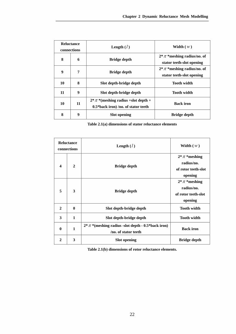
equation 2.2.12 with the values given in table 2.1.
(a): a typical reluctance mesh discretisation. (b): mesh numbering
Figure 2.2.6 A typical induction machine reluctance mesh discretisation
Chapter 2 Dynamic Reluctance Mesh Modelling
22
Reluctance connections
Length ( l ) Width ( w )
8 6 Bridge depth 2*π *meshing radius/no. of
stator teeth-slot opening
9 7 Bridge depth 2*π *meshing radius/no. of
stator teeth-slot opening
10 8 Slot depth-bridge depth Tooth width
11 9 Slot depth-bridge depth Tooth width
10 11 2*π *(meshing radius +slot depth +
0.5*back iron) /no. of stator teeth Back iron
8 9 Slot opening Bridge depth
Table 2.1(a) dimensions of stator reluctance elements
Reluctance connections
Length ( l ) Width ( w )
4 2 Bridge depth
2*π *meshing radius/no.
of rotor teeth-slot opening
5 3 Bridge depth
2*π *meshing radius/no.
of rotor teeth-slot opening
2 0 Slot depth-bridge depth Tooth width
3 1 Slot depth-bridge depth Tooth width
0 1 2*π *(meshing radius -slot depth - 0.5*back iron)
/no. of stator teeth Back iron
2 3 Slot opening Bridge depth
Table 2.1(b) dimensions of rotor reluctance elements.

Chapter 2 Dynamic Reluctance Mesh Modelling
23
(a) stator dimensions (b) rotor dimensions
Figure. 2.2.7 Induction machine stator and rotor dimensions
Although this is the typical reluctance mesh used for induction machines, it
could also be applied to other machine types that have similar rotor or stator
geometries and flux distribution characteristics. A similar reluctance mesh will
be employed for the stator of salient pole synchronous generators later in chapter
4.
2.2.3 Dynamic reluctance mesh creation of electrical machines: the air gap
In a simple magnetic circuit as shown in figure 2.2.8, where there is an air gap
in the magnetic circuit, the equivalent magnetic circuit can be derived as shown
in figure 2.2.8.
Figure 2.2.8 A simple air gap magnetic circuit includes air gap

Chapter 2 Dynamic Reluctance Mesh Modelling
24
Because the permeability of air is much smaller than that of iron, the flux is
well confined to the iron path rather than leaking into air, as has been discussed
in section 2.2.1. In a magnetic circuit where an air gap exists, as in figure 2.2.8,
most of the flux enters the air gap from the iron perpendicularly to the iron
surface. However, in practice, the magnetic field lines actually ‘fringe’ slightly
outward as they cross the air gap [24], as shown in figure 2.2.9. This fringing
field will increase the ‘effective’ cross-sectional area of air gap elements in a
magnetic circuit analysis. There are several empirical ways of coping with this
fringing effect and they will be introduced later in chapter 3. For the time being
this fringing effect will be neglected and the area of the air gap element is taken
to be equal that of the adjacent iron element.
Figure 2.2.9 Air gap in a simple magnetic circuit
The air gap plays a very important role in magnetic circuit analysis, because
most of the mmf is dropped across the air gap. This is because the permeability
of air is very small and thus the air gap reluctance is large compared to the iron
reluctances. In electrical machines, the air gap is paramount in determining the
energy conversion processes and thus modelling the air gap properly is a key
factor in simulating electrical machine performance accurately.
To properly represent the flux paths between each pair of stator and rotor teeth,
air gap reluctances connecting each pair of stator and rotor teeth are introduced
in the magnetic circuit of electrical machines, as shown in figure 2.2.10.
Chapter 2 Dynamic Reluctance Mesh Modelling
25
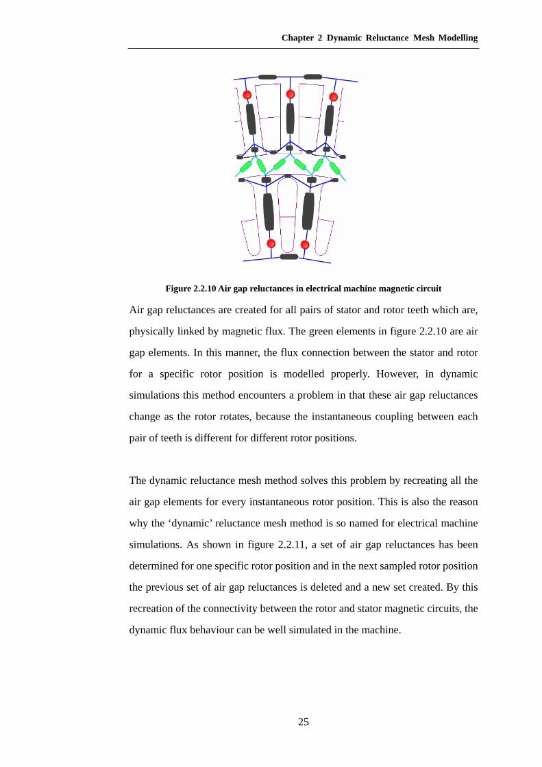
Figure 2.2.10 Air gap reluctances in electrical machine magnetic circuit
Air gap reluctances are created for all pairs of stator and rotor teeth which are,
physically linked by magnetic flux. The green elements in figure 2.2.10 are air
gap elements. In this manner, the flux connection between the stator and rotor
for a specific rotor position is modelled properly. However, in dynamic
simulations this method encounters a problem in that these air gap reluctances
change as the rotor rotates, because the instantaneous coupling between each
pair of teeth is different for different rotor positions.
The dynamic reluctance mesh method solves this problem by recreating all the
air gap elements for every instantaneous rotor position. This is also the reason
why the ‘dynamic’ reluctance mesh method is so named for electrical machine
simulations. As shown in figure 2.2.11, a set of air gap reluctances has been
determined for one specific rotor position and in the next sampled rotor position
the previous set of air gap reluctances is deleted and a new set created. By this
recreation of the connectivity between the rotor and stator magnetic circuits, the
dynamic flux behaviour can be well simulated in the machine.

Chapter 2 Dynamic Reluctance Mesh Modelling
26
Figure 2.2.11 Dynamic creations of air gap reluctances in DRM method
For other types of machines, which have non-uniform air gap geometry, such as
salient pole synchronous generators, a different method of evaluating the air gap
reluctances may be used, but the concept of dynamic creation – destruction of
elements remains the same. Chapter 4 will discuss the non-uniform air gap
reluctance calculations in detail.
2.2.4 Dynamic reluctance mesh method of electrical machines: torque
calculation
In the DRM method, torque is calculated based on the principle of virtual work
[3][4], that is flexible, easy to apply and does not require knowledge of the
mutual flux components in the air gap. This is an alternative method to
Maxwell’s tensor formulation. The force and torque are obtained from the
derivatives of the energy (co-energy) versus the displacement of the movable
part. Specifically for electrical machines, the torque is calculated by evaluating
the net change in stored and supplied energy due to an incremental virtual
rotation of the rotor if the fluxes remain constant over the change. In the DRM,
this procedure is greatly simplified by noting that the only position-dependent
elements are those in the air gap and therefore the net torque is given by

Chapter 2 Dynamic Reluctance Mesh Modelling
27
∑−
= ∂∂
=1
0
N
i
ie
ETθ
(2.2.20)
where N is the number of air gap reluctances created in this specific rotor
position, and iE is the energy stored in each air gap element.
Energy stored in a magnetic field over the volume V [24]:
∫ ∫ ⎟⎠⎞⎜
⎝⎛ ⋅=
V
BdVdBHE
0 (2.2.21)
For soft magnetic material of constant permeability where HB µ= equation
2.2.21 evaluates to [24]:
dVBEV∫ ⎟⎟
⎠
⎞⎜⎜⎝
⎛=
µ2
2
(2.2.22)
In DRM method, the stored magnetic energy in each air gap reluctance in which
B is assumed uniform is:
VBVolumnHBEenergy ⋅=⋅⋅⋅=0
2
221
µ (2.2.23)
and therefore the total electrical torque is:
∑∑∑−
=
−
=
−
=⎟⎟⎠
⎞⎜⎜⎝
⎛∂∂⋅⋅=⎟⎟
⎠
⎞⎜⎜⎝
⎛∂∂⋅⋅=
∂
⎟⎟⎠
⎞⎜⎜⎝
⎛⋅∂
=1
0 0
21
0 0
21
0
0
2
21
212 N
i
iiiiN
i
iiN
i
i
ii
ewldBVB
VB
Tθµθµθ
µ (2.2.24)
where iB is the flux density in the thi air gap reluctance, and id , il , iw , iV are the
depth, length, width and volume of this air gap reluctance.
2.2.5 Dynamic Reluctance Mesh method of electrical machines: skew
modelling
In previous sections of this chapter, the creation of a typical reluctance mesh for
induction machines has been implemented and now a further practical issue for

Chapter 2 Dynamic Reluctance Mesh Modelling
28
machine simulations, namely skewed rotor simulations, will be introduced in
this section.
Most cage induction motors have their rotor slots skewed by one slot-pitch to
reduce space harmonics in the air gap flux density introduced by the slotting
[25]. Because of its 3D nature, consideration of skew has generally involved
significant computational effort in electrical machine simulations. The DRM
uses a quasi-3D method to model skew. Dividing the whole machine into several
sections along its axial length, each section is offset by a small angle with respect
to the previous section to model the skew, as shown in figure 2.2.12. The DRM
approach assumes that the axially directed flux is negligible such that the
reluctances meshes of different axial sections are only coupled indirectly
through the rotor and stator electrical circuits.
Figure 2.2.12 Skew model of cage rotor Figure 2.2.13 Trapezoidal rotor tip elements
Figure 2.2.13 shows the relative position of the stator and rotor in different skew
sections. As stated above, the machine has been divided into several skew
sections and the reluctance meshes for both the stator and rotor are separately
generated for each section including air gap reluctances.
In figure 2.2.13, the overlapping area between pairs of stator and rotor teeth is
rectangular in this case and thus the appropriate reluctance connects the

Chapter 2 Dynamic Reluctance Mesh Modelling
29
corresponding stator and rotor nodes has a rectangular cross-section. However,
this way of calculating air gap reluctance values has two disadvantages [3].
Firstly, it is clear that the more skew sections that are used; the more accurate
the effects of skew are modelled. Unfortunately the more skew sections that are
used the longer the calculation time. Secondly, when rotating at constant speed,
the overlap area between a pair of rotor and stator teeth is a piecewise linear
function of time. Unfortunately, the evaluation of the torque generated by the
motor in equation 2.2.24 depends upon the rate of change of these reluctances
with time and this causes discontinuous steps in the torque. Not only does this
appear as unwanted numerical ‘noise’, but also it has a noticeable effect on the
ease with which the simulation can predict the future state of the machine from
the present one and hence the calculation time required for the simulation to go
forward in time.
To address both of the issue, the DRM model uses trapezoidal shape rotor tip
elements in the skewed rotor model, as shown in figure 2.2.14.
Figure 2.2.14 Trapezoidal air gap elements in DRM modelling
By using the trapezoidal elements for air gap elements in a skewed rotor
machine, the rate of change of the air gap reluctances is always continuous and
the problems caused by discontinuities in the torque are avoided. Figure 2.2.15
shows the torque ripple observed in the simulation of the direct on line start of
an unloaded induction machine. It can be seen that the use of trapezoidal skew

Chapter 2 Dynamic Reluctance Mesh Modelling
30
elements significantly reduces the unphysical torque ripple seen when using
rectangular elements.
Torque in induction machine
-600
-400
-200
0
200
400
600
800
1000
1200
0 0.05 0.1 0.15 0.2
Time(s)
Tor
que
(N.m
)
rectangular shape elements trapezoidal shape elements
rectangular shape elements
trapezoidal shape elements
Figure 2.2.15 Torque ripple comparison for the result come from induction machine direct
on line start no load condition simulation, with air gap modelled by rectangular and trapezoidal shape elements
Number of iterations
-50
0
50
100
150
200
250
0 0.05 0.1 0.15 0.2
Time (s)
Num
ber
of it
erat
ion
rectangular shape elements trapezoidal shape elements
rectangular shape elementstrapezoidal shape elements
Figure 2.2.16 Number of iteration comparison for the results come from induction machine direct on line start no load condition simulation, with air gap modelled by
rectangular and trapezoidal shape elements
Figure 2.2.16 shows the number of iterations required in the Newton-Raphson
solver, which will be discussed later in this chapter. It can be seen that the use of

Chapter 2 Dynamic Reluctance Mesh Modelling
31
trapezoidal shape elements requires slightly fewer iterations compared to the
use of rectangular elements. Quantitatively, the average number of iterations for
rectangular elements is 23.83, compared to 19.32 for trapezoidal elements.
Employing trapezoidal shape elements reduces the unphysical numerical noise
and total computational time of induction machine simulations.
Further details about the air gap modelling technique in skewed rotor induction
machines will be presented in chapter 3 along with some other approaches for
coping with skew.
2.3 State Variables and State Equations
In the previous sections of this chapter the methodology for discretising the
induction machine geometry into reluctance meshes was discussed as well as
the method to calculate torque and to deal with skewed rotors. This section will
describe how the system state is defined and present the system equations, which
govern the system’s behaviour.
As discussed in section 2.2.1, flux conservation holds at a ‘node’ in a magnetic
circuit in an analogous manner to KCL in an electric circuit. In a dynamic
simulation, conservation of flux at each ‘node’ for every specific time instance
should be enforced. As can be seen from equation 2.2.13, the magnetic flux
flowing through the reluctance can be evaluated given the mmf drop across it
and its reluctance value. The DRM model specifies each node’s mmf value as a
state variable and conservation of the rate of change of flux is enforced at each
node. An initial condition for the mmf value, which is typically zero, is also
given. For each node i , conservation of the net rate of change of flux entering it
from all the elements connecting to this node holds, as shown in equation 2.3.1,
and in figure 2.3.1:

Chapter 2 Dynamic Reluctance Mesh Modelling
32
( ) 0, 12
1
0=∑
−
=jjji
n
jmmfmmf
dtd φ (2.3.1)
where n is the number of elements connected to this node, and jiφ is the flux
flowing through the thj element to the thi node as a function of the node
potentials, 2jmmf and 1jmmf .
Figure 2.3.1 Conservation of rate of change of flux in one node
The instantaneous rate of change of flux through each mesh element is
calculated from
⎥⎦
⎤⎢⎣
⎡⎟⎠⎞
⎜⎝⎛
ℜ∆−∆
−⎟⎠⎞
⎜⎝⎛
ℜ∆+∆
∆=
)2/()2/(1 ttFttFtdt
dφ (2.3.2)
Equation 2.3.2 forms the basis for a non-linear set of equations, the source terms
which are obtained by linking the above magnetic model with a lumped element
electrical circuit model for the machine windings. Consider the simple electrical
loop supplied by a voltage source as shown in figure 2.3.2 below.
Figure 2.3.2 Coupling of a single turn electrical network with the reluctance mesh
The existence of the electrical current in the loop is incorporated into the
magnetic circuit via the mmf source terms as discussed in the previous sections.

Chapter 2 Dynamic Reluctance Mesh Modelling
33
The induced electromotive (emf) in the loop is determined by the rate of change
of flux in the corresponding mmf source (which clearly ensures conservation of
power). Applying KVL around the electrical circuit loop yields
dttd
dttdiLtiRtv Lcu
)()()()( φ++= (2.3.3)
In equation 2.3.3, copper loss is incorporated as a resistor, cuR , and an inductive
term is introduced to allow for any end winding leakage reactances which are
not explicitly modelled in the DRM. The driving term in equation 2.3.3 is the
applied voltage.
Naturally, realistic windings for practical machines are not just simple loops but
are specifically designed to obtain an mmf distribution in the air gap region
which is as close to sinusoidal as possible. Thus, practical machine windings are
usually singly or doubly wound. For example in a three-phase induction motor,
the stator electrical equations would be of the form:
∑=
⋅+⋅=S
i
i
i
aaaA dt
dddeiRv
1
φφ
(2.3.4)
∑=
⋅+⋅=S
i
i
i
bbbB dt
dddeiRv
1
φφ
(2.3.5)
∑=
⋅+⋅=S
i
i
i
cccC dt
dddeiRv
1
φφ
(2.3.6)
Where Av , aR and ai are the applied voltage source, resistance and current of
phase A respectively. S is the number of stator teeth. i
a
ddeφ
is the term
representing the change of the emf induced in phase A due to a change of flux in
tooth i . These expressions account for the total flux linkage changes that are
enclosed by the phase A electrical loop and implicitly involve the connectivity
between the electrical network and the magnetic circuit as defined by the
winding pattern.

Chapter 2 Dynamic Reluctance Mesh Modelling
34
Figure 2.3.3 Coupling of electrical network and magnetic circuit in a cage rotor
In a cage rotor, as shown in figure 2.3.3, these electrical loop equations are
modelled to 011 =−⋅+⋅− −− dtdRiRi iiiiφ , where ii and 1−ii are currents in bar i
and bar 1−i , and φ is flux passing between them. The relationship between
the currents and the mmf is shown in equation 2.3.7. According to Ampere’s
law, the current flowing through each bar is determined by the mmf difference
for adjacent bars.
iii mmfmmfi −= +1 (2.3.7)
Thus, these mmf sources, immf in each bar are employed as state variables in
the DRM model for induction machines, as shall be seen later in this chapter.
The above equations define the electrical and magnetic response of the machine.
Dynamic simulations of a machine require consideration of the mechanical
response, as defined by:
0=−dt
d mechr
θω (2.3.8)
0=−−− loadrr
e TDdt
dJT ωω (2.3.9)
where rω is the mechanical speed of the rotor and D and J are the
associated machine windage and inertia respectively.
To summarize, the variables that characterise the machine’s state and for which
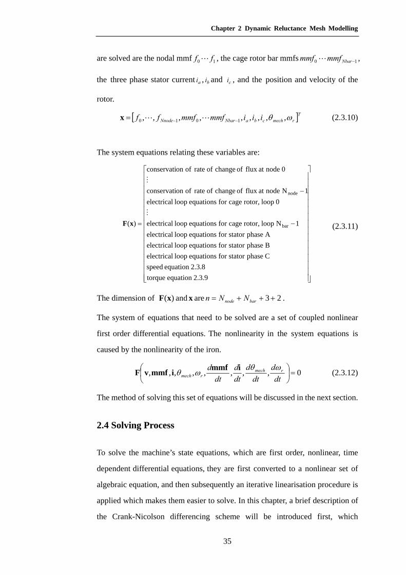
Chapter 2 Dynamic Reluctance Mesh Modelling
35
are solved are the nodal mmf 10 ff L , the cage rotor bar mmfs 10 −Nbarmmfmmf L ,
the three phase stator current ai , bi and ci , and the position and velocity of the
rotor.
[ ]TrmechcbaNbarNnode iiimmfmmfff ωθ ,,,,,,,,, 1010 −−= LLx (2.3.10)
The system equations relating these variables are:
⎥⎥⎥⎥⎥⎥⎥⎥⎥⎥⎥⎥⎥⎥⎥⎥
⎦
⎤
⎢⎢⎢⎢⎢⎢⎢⎢⎢⎢⎢⎢⎢⎢⎢⎢
⎣
⎡
−
−
=
2.3.9equation torque2.3.8equation speed
CphasestatorforequationsloopelectricalBphasestatorforequationsloopelectricalAphasestatorforequationsloopelectrical
1Nlooprotor,cageforequationsloopelectrical
0looprotor,cageforequationsloopelectrical1Nnodeatflux of change ofrateofonconservati
0nodeatflux of change ofrateofonconservati
)( bar
node
M
M
xF (2.3.11)
The dimension of )(xF and x are 23+++= barnode NNn .
The system of equations that need to be solved are a set of coupled nonlinear
first order differential equations. The nonlinearity in the system equations is
caused by the nonlinearity of the iron.
0,,,,,,,, =⎟⎠⎞
⎜⎝⎛
dtd
dtd
dtd
dtd rmech
rmechωθ
ωθ immfimmfvF (2.3.12)
The method of solving this set of equations will be discussed in the next section.
2.4 Solving Process
To solve the machine’s state equations, which are first order, nonlinear, time
dependent differential equations, they are first converted to a nonlinear set of
algebraic equation, and then subsequently an iterative linearisation procedure is
applied which makes them easier to solve. In this chapter, a brief description of
the Crank-Nicolson differencing scheme will be introduced first, which

Chapter 2 Dynamic Reluctance Mesh Modelling
36
converts the nonlinear differential equation to nonlinear algebraic equations,
and then the Newton-Raphson method, which linearises these nonlinear
equations, will be introduced. The overall solution procedure will be given
finally in this section on a flow chart.
2.4.1 Crank-Nicolson differencing scheme
The Crank-Nicolson differencing scheme is adopted here to convert the
differential equations into algebraic equations. The Crank-Nicolson method is
an implicit differencing scheme with second-order accuracy that allows larger
time steps [23] than explicit schemes. It is a compromise between the Forward
Time Centre Space (FTCS) method [23] and the Fully Implicit method. The
FTCS differencing scheme is first-order accurate but only stable for sufficiently
small time steps, whereas the Fully Implicit scheme is stable for arbitrary large
time steps, is only first-order accurate, but generally requires matrix solvings.
The reason why the Crank-Nicolson has been chosen for the DRM code is due
to its well-proven stability and accuracy. There is a parameter α in the
differencing scheme which balances the scheme between implicit and explicit.
The factor 5.0=α corresponds to the Crank-Nicolson scheme. For each time
step the Crank-Nicolson approach approximates the variables’ value and time
derivatives:
( ) ( )ttttt ∆+−+=⎟⎠⎞
⎜⎝⎛ ∆+ xxx )1(
2αα
( ) ( )t
tttttdtd
∆−∆+
=⎟⎠⎞
⎜⎝⎛ ∆+
xxx2
(2.4.1)
Although choosing α =0.5 provides the most accurate results it is on the
stability limit. In practice, a slightly different lower value forα , such as 0.495,
is used to make the system slightly implicit which overcomes any instability
caused by numerical noise such as rounding errors.

Chapter 2 Dynamic Reluctance Mesh Modelling
37
Applying the differencing scheme of equations 2.4.1 yields
⎟⎟⎟⎟⎟⎟
⎠
⎞
⎜⎜⎜⎜⎜⎜
⎝
⎛
=
⎟⎟⎟⎟⎟⎟
⎠
⎞
⎜⎜⎜⎜⎜⎜
⎝
⎛
∆+∆+∆+∆+∆+
)()()()()(
)()()()()(
ttttt
tttttttttt
ωθ
ωθ
IFV
BIFV
A (2.4.2)
where A and B are sparse, as yet nonlinear, matrix. Given the present value of
the state variables those at the next time step can be found from equations 2.4.2.
The rest of the section will describe how the nonlinear behaviour is iteratively
linearised.
2.4.2 Newton-Raphson multidimensional nonlinear solving technique
Multi-dimension simultaneously nonlinear equations are difficult to solve, in
that it is difficult to find the solution that sets all of the system equations to
zero. For example, consider two dimensional nonlinear equations which need
to be solved simultaneously,
0),(0),(
==
yxgyxf
(2.4.3)
The functions ),( yxf and ),( yxg are two arbitrary nonlinear equations and
they both divide the xy plane into positive and negative parts, as shown in
figure 2.4.1.

Chapter 2 Dynamic Reluctance Mesh Modelling
38
Figure 2.4.1 [23] Solutions of two nonlinear equations. The grey regions are the
positive regions for the function f and the dashed lines divide the plane into positive and negative regions for the system
From figure 2.4.1 it can be seen that to solve the system with two equations,
the intersections of the zero contour lines of the function f and g have to
be found. Since normally function f and g are unrelated, this is not a simple
task.
For multi-dimensional equations this task becomes even more complicated.
Our aim is to find the common solutions, the roots to all of the equations, i.e.
the intersection of all the zero contours in N-dimensional space which is
generally difficult if no insight into the nature of the problem can be obtained
in advance.
In the DRM modelling the simplest multi-dimensional solving technique, the
Newton-Raphson method, is used. This method provides a very efficient means
of converging to a root if an initial guess is sufficiently good.
For example consider one-dimensional nonlinear root-finding problem solved
by Newton-Raphson. To solve the problem 0)( =xf , a taylor series for )(xf
is expanded in the neighbourhood of an estimation ( x ) to the solution 0x :

Chapter 2 Dynamic Reluctance Mesh Modelling
39
L+′′
+′+=+ 2
2)()()()( δδδ xfxfxfxf (2.4.4)
where x is the current estimation to the solution 0x , and δ is the distance
between the current estimation and the next estimation. For sufficiently small
enough values ofδ and a well-behaved function, terms higher than linear are
not important, and thus if the root occurs at δ+x
0)( =+ δxf (2.4.5)
which gives:
)()(
xfxf′
−=δ (2.4.6)
If the function value )(xf and its derivative )(xf ′ at the estimation point are
known, where x is a suitable estimate to solution 0x , then δ is evaluated
from equation 2.4.5 and a better estimate of x found. Geometrically speaking,
as can be seen from figure 2.4.2, Newton’s method extends the tangent line at
point x until it cross the x axis which becomes the next predicted value of the
system solution; this procedure continues until the function value is small
enough to be regarded as zero, as shown in figure 2.4.2.
Figure 2.4.2 [23] Newton method in one dimensional to find the next predicted value
However, although Newton’s method for one-dimensional problems is fast and
effective, it will fail to converge if the initial point is not close enough to the
solution (figure 2.4.3), or the system function has local extremes (figure 2.4.4)
where high order terms in equation 2.4.4 are important.

Chapter 2 Dynamic Reluctance Mesh Modelling
40
Figure 2.4.3 [23] Initial guess is not close enough to the solution and nonconvergence
situation happened in Newton-Raphson method
Figure 2.4.4 [23] Newton-Raphson method encounters a local extreme where high order
terms are important and cannot be neglected
The Newton-Raphson method can be used in multidimensional root finding
problem and is very efficient to converge to a root, if the initial guess is
sufficiently good [23]. An improved Newton-Raphson solving technique will
be introduced later in chapter 3, which gives a global convergent
Newton-Raphson method no matter where the initial guess is.
In a one-dimensional problem, the function value )(xf and its
derivative )(xf ′ at point x are needed in order to calculate the next predicted
root. In multi-dimensional problems the value of the equations for a system
state x and the system Jacobian matrix at x are needed. The Jacobian matrix is
the first partial derivative matrix of the system equations with respect to the

Chapter 2 Dynamic Reluctance Mesh Modelling
41
state variables as given in equation 2.4.7.
⎥⎥⎥⎥⎥⎥⎥⎥⎥
⎦
⎤
⎢⎢⎢⎢⎢⎢⎢⎢⎢
⎣
⎡
∂∂
∂∂∂∂
∂∂
∂∂∂∂
∂∂
∂∂∂∂
=∂∂
≡
n
n
n
n
nn
j
iij
xf
xfxf
xf
xfxf
xf
xfxf
xFJ
M
L
L
L
L
MM
2
1
2
2
2
2
1
1
1
2
1
1
(2.4.7)
where x denotes the vector value of system variants and F denotes the vector
of function values.
Consider the multi-dimensional system equations in the DRM modelling, as
shown in equation 2.4.8. The Newton-Raphson expansion for the thi equation
is:
( ) ( ) ( )21
0
,,,, xxxFxxFxxxxF j
N
j j
ijiijjiii δδδδ Ο+
∂∂
+=++ ∑−
=
LL (2.4.8)
In matrix notation, the above function is:
( ) ( ) ( )2xxJxFxxF δδδ Ο+⋅+=+ (2.4.9)
where J is the Jacobian matrix defined in equation 2.4.7.
If terms of order 2xδ and higher terms are neglected, and the root occurs
at xx δ+ , then the correction xδ that moves the solution toward the root is:
FxJ −=⋅δ (2.4.10)
xxx oldnew δ+= is the process to be iterated to converge.
Thus application of the Newton-Raphson scheme linearises the system
equations. In the next section, the approach used to solve these linear equations
will be discussed.
Chapter 2 Dynamic Reluctance Mesh Modelling
42
2.4.3 Linearised equation solving method
The linear equations 2.4.10 above are inherently sparse because the majority
are derived from the magnetic reluctance mesh circuit. Previous work [1][26]
has solved these linearised equations by LU decomposition, a direct matrix
method which becomes rapidly untenable as the size of the problem increases,
i.e. with the number of reluctances used in the discretisation of the magnetic
circuit of the electrical machine.
The alternative approach adopted in DRM modelling, is to use an iterative
method such as the preconditioned Bi-Conjugate Gradient Stabilised
(BiCGSTAB) algorithm in conjunction with efficient sparse matrix-vector
multiplications [27]. Due to the irregular sparse matrix involved in the system
equations, a simple pre-processing routine is included as a preconditioner to
increase the convergence of the iterative process. The preconditioner used is a
simple incomplete LU decomposition. The linear equations FxJ −=⋅δ are
preconditioned as
FJxJJ 11 ⋅−=⋅ −− ~~ δ (2.4.11)
where 1J −~ is the approximate inverse matrix of J identified by incomplete LU
decomposition, so that IJJ ≈⋅−1~ . Incomplete LU decomposition uses a partial
decomposition scheme where the appearance of elements in the inverse matrix
is controlled by a threshold, only those elements of magnitude above the
threshold appear in the inverse matrix. By applying different thresholds, the
program can vary the accuracy to the true inverse matrix of J which allows a
balance between memory use and computation time. The smaller the threshold,
the greater the memory usage, but the better preconditioned the matrix problem
which requires fewer iterations of the linear solver i.e. the BiCGSTAB solver.
However, insufficient preconditions may lead to a total failure to converge. A
schematic relationship diagram between memory usage and the number of

Chapter 2 Dynamic Reluctance Mesh Modelling
43
iterations in the BiCGSTAB linear solver with respect to the threshold is shown
in figure 2.4.5.
Figure 2.4.5 Schematic diagram shown the relationship between memory usage and the
number of linear solver iteration with respect to threshold
After the nonlinear first order differential system equations are solved by the
algorithms introduced above, the system state at a specific time is known. As
the Newton-Raphson nonlinear solving scheme needs an initial guess for the
solving process at each time instance, a prediction for next time step is
calculated. This is based upon the present solution and it is different from the
previous step.
)( previouspresentpresentpredicted xxxx −+= (2.4.12)
However, as has been discussed in section 2.4.2 and shown in figure 2.4.3, the
Newton-Raphson method is sensitive to the initial guess, and will fail to
converge if the initial guess is not sufficiently good. In electrical machine
simulations, most of the nonlinearity in the machine is due to the nonlinear
characteristic of the iron material. If, at some time instance when the flux
density value in a part of the iron is around the ‘knee’ area of its B-H curve, the
system equations exhibit a dramatic degree of nonlinearity, which undermines
the NR process.
To alleviate this, the DRM employs a simple scheme to try to ensure the

Chapter 2 Dynamic Reluctance Mesh Modelling
44
robustness of solving process, the use of an adaptive time step method. If at
one time step, the Newton-Raphson scheme fails, the system state will be reset
to that of the previous time step and the time step used is halved and a new
predicted value using the halved time step will be calculated. The
Newton-Raphson scheme will then attempt to solve the system state in the new
time step and, if it fails again, the same process continues until the
Newton-Raphson succeeds. If, on successful convergence the time step is
doubled and subject to remain less than a predefined maximum value.
The criteria used to decide whether the solution process for the current time
step is unsuccessful is that:
1. The total equation error on iteration of the Newton-Raphson process
increases compared to the previous iteration;
2. The conjugate gradient solver (BiCGSTAB) fails to solve the linear
equations in a predefined number of iterations;
As just described the time step is then halved and the whole machine state will
be recovered to the previous time step.
The total system error in the solving process is defined as
( )
N
xFError
N
ipresenti
total
∑−
==
1
0
2
(2.4.13)
2.4.4 The DRM program flow chart
In section 2.4, the system solving techniques have been discussed. Now the
DRM system flow chart will be given to show a clear view of the program
structure, as shown in figure 2.4.6.

Chapter 2 Dynamic Reluctance Mesh Modelling
45
START
Load machine parameters, stator and rotormesh segments
Replicate mesh segments to wholemachine slice
Replicate each slice with skew angle tomodel skewed rotor
Stator winding specifications
Renumbering nodes for coding reasons,initialize machine state variables
Load simulation parameters: threshold,tolerance, time step etc.
preprocessor
A
(a) DRM Preprocessor flow chart

Chapter 2 Dynamic Reluctance Mesh Modelling
46
Each time steploop
Time=time+dt
Obtain drivingvoltages for stator
Newton-Raphsonloop
Create air gap elements for this specificrotor position
Calculate system equations?total error andJacobian matrix
Totalerror<tolerance
Linear solver- preconditioned ConjugateGradient solver (BiCGSTAB)
Obtain system solutions based on thecorrection from linear solver
Delete air gap elments
No. iteration> max iteration?Error>0.5*previous error?
Linear solver faulty?
Error>tolerance?
Clear linearsolver object
Restart: half timestep, restoresystem state
Write results to file
Solving process
Yes
No
Yes
No
No
Yes
A
BC
(b) DRM solving core flow chart

Chapter 2 Dynamic Reluctance Mesh Modelling
47
Predict the initialguess of next time
step
If dt>dtmaxdt=dtmax
END
Simulation timereached?
Post-processor
No
Yes
C B
(c) DRM post-processor flow chart
Figure 2.4.6 DRM program flow chart
The total system flow chart is shown in figure 2.4.6. It can be seen that the
whole DRM program is divided into three parts, which are the pre-processor,
the solving core and the post-processor.
The pre-processor sets up the dynamic magnetic reluctance mesh model of the
machine. It reads in the machine geometry, the winding arrangements and the
simulation parameters, such as the threshold and maximum simulation time
step. In creating the reluctance mesh, the pre-processor reads the mesh
topology of one pair of stator teeth first and then replicates these through the
whole machine to get the complete reluctance mesh. The same replication
procedure happens to create the rotor reluctance mesh. Skewed rotor is also
implemented by replicating the reluctance mesh in one skew section to the
other skew sections with the appropriate angular offsets. Due to the dynamic
creation of air gap elements which depends upon the specific position of the
rotor, and thus vary for each time step, the DRM leaves these to the solution
phase.

Chapter 2 Dynamic Reluctance Mesh Modelling
48
In the main solving core, the system state is solved for each time step. It can be
seen that in each time step, air gap reluctances for this specific rotor position
are created and the system state equations are evaluated. If the current system
state is close enough to the exact system solution, i.e. total system error are
smaller than the tolerance, solving process for the current time step will be
stopped and the current state will be taken as the exact solution, and the
program carries on to next time step solving process. However, if the system
equation error for the current time step is not small enough, the preconditioned
iterative linear solver (BiCGSTAB) will be invoked to solve for the next
Newton-Raphson solution in current time step. After solving for the next
Newton-Raphson solution for current time step, air gap elements will be
deleted. After that, the system will check to see if the Newton-Raphson solving
process has failed. If the Newton-Raphson fails, the time step will be reduced
and the whole system state will be restored to the previous time step, then a
new system state prediction will be generated based on the reduced time step.
If the Newton-Raphson solving process is healthy in the current step, the total
system error is checked to decide if this next Newton solution coming out of
the linear solver is accurate enough, by applying the criteria given in section
2.4.3. This procedure will continue until the total system equation error is
smaller than the tolerance, i.e. to find the exact system solution for this current
time step.
The postprocessor writes out the simulation results and predicts the solution of
the next time step which is regarded as the initial guess for the
Newton-Raphson algorithm.
2.5 Conclusion
This chapter described the Dynamic Reluctance Mesh modelling method for
electrical machines. Since it is based upon magnetic circuit theory, a brief

Chapter 2 Dynamic Reluctance Mesh Modelling
49
introduction of the basic theory of magnetic circuits was first given, and then
the procedure for creating dynamic reluctance meshes for electrical machines
taking the induction machine as an example, was presented. The description of
the DRM emphasised the descritisation method of the iron and air parts of the
machine and the way the DRM deals with skewed rotors and torque
calculations are also described. After the reluctance model has been defined for
the induction machine, the chapter summarised the system state variables and
system equations describing the induction machine electro-mechanical system.
Section 2.4, detailed how the system state is solved in the DRM, including the
Crank-Nicolson scheme, Newton-Raphson iterations and the preconditioned
BiCGSTAB linear solver. The flow chart for the solution process is also given.

Chapter 3 Developments of The Dynamic Reluctance Modelling Software
50
CHAPTER 3 DEVELOPMENTS OF THE DYNAMIC
RELUCTANCE MODELLING SOFTWARE
3.1 Introduction
Dynamic Reluctance Modelling is a fast and effective method of modelling
electrical machines as has been described and validated by Sewell [3] for cage
induction machines. However, with the increased requirements upon
simulations of electrical machines, more detailed models are needed to
accommodate the complex flux distributions in the air gap regions due to the
complicated tooth geometry and fringing effects. Thus, some improvements
have been made to enhance the modelling of the air gap elements.
Moreover, scheme solving the system equations using Newton-Raphson
iterations coupled with the Crank-Nicolson technique works well for a single
cage induction machine, as has been described in chapter 2 where the
nonlinearity only exists in iron materials. However, the situation becomes more
complicated if there are other nonlinear components involved in the system,
such as the rotating rectifiers which exist in brushless generating systems.
Some modifications have to be made to strengthen the Newton-Raphson
solving process, in order to cope with the higher degree of system nonlinearity
and the deficiency of the Newton-Raphson algorithm already presented in
chapter 2.
This chapter states the modifications that have been made to the original
version of the Dynamic Reluctance Modelling software and why these changes
have been made. Section 3.1 describes the detailed modelling method of air
gap elements; section 3.2 describes the changes of nodal flux equations;

Chapter 3 Developments of The Dynamic Reluctance Modelling Software
51
chapter 3.3 presents the modified globally convergent Newton-Raphson
nonlinear solver. Finally, further modifications were made to the induction
machine model to make it more precise and a comparison of results between
Finite Element models and the Dynamic Reluctance Mesh models is also
given.
3.2 Representing Air Gap Reluctances Precisely
Magnetic equivalent circuits are more difficult to derive than electrical
equivalent circuits from the field point of view due to the relatively large
leakage phenomenon in magnetic paths: in electrical circuits, most of the
current caused by moving electrons can be constrained within electrical
conducting materials and components, because the electrical conduction of air
is extremely small compared to that of metals. In magnetic circuits, things are
quite different. The permeability of air is not insignificant compared to that of
magnetic materials and therefore the flux paths are difficult to predict and
calculate as flux can ‘leak’ out of the magnetic path, as depicted in chapter 2 by
the air gap fringing effect shown in figure 2.2.9. This leakage of flux in the air
gap region causes difficulties for modelling in electrical machines and these
fringing effects are reflected as a modified air gap reluctance width or length.
There are several ways of dealing with these air gap reluctance issues in a
computer code, either taking the fringing effect into account or not. These
options will be introduced in turn.
3.2.1 Method 1
The method of calculating the air gap reluctance element values, which has
been introduced in chapter 2, is called Method 1 in this thesis. It utilises a
relatively simple way of modelling the air gap elements assuming that the flux
across the air gap region between the stator and rotor is normal to both the

Chapter 3 Developments of The Dynamic Reluctance Modelling Software
52
stator and rotor tooth surfaces and calculates the area of air gap elements using
the direct overlap area of each pair of stator and rotor teeth, as shown by the
shadowed area in figure 3.2.1.
Figure 3.2.1 Air gap modelling in DRM: method 1
When allowing for skewed rotors, the air gap reluctance values in each skew
section are evaluated for a trapezoidal overlap area, for reasons which are
already explained in chapter 2.
Now a detailed analysis of how the overlap area is calculated in each skew
section will be given. Figure 3.2.2 (a) shows the overlapped air gap area for a
non-skewed rotor which is the rectangular area between a pair of rotor and
stator teeth.
Figure 3.2.2 Air gap elements calculated by method 1
(a) non-skewed rotor; (b) skewed rotor
However, for the skewed section of induction machine shown in figure 3.2.2

Chapter 3 Developments of The Dynamic Reluctance Modelling Software
53
(b), the overlap area between the stator and rotor teeth are more difficult to
calculate. The air gap reluctance area is evaluated from the irregular overlap
area shown in figure 3.2.3(b).
As mentioned in chapter 2, the air gap reluctance effective width is a
piece-wise linear function of time. The width changes as the rotor rotates. The
figures shown in figure 3.2.3 encompass the possible configurations.
Figure 3.2.3 Different stator and rotor overlap conditions in a skewed rotor section
Figure 3.2.4 plots the effective air gap reluctance width between a pair of stator
and rotor teeth plotted with respect to their relative position. It can be seen
from these curves that, the more the displacement (relative position between a
pair of stator and rotor teeth), the less the width of the air gap reluctance
connecting this pair of teeth. There are five curves in figure 3.2.4, each of them
has a skewed rotor with different rotor skew angles, from 0.01 mechanical
degree to 15 degree.

Chapter 3 Developments of The Dynamic Reluctance Modelling Software
54
Air Gap Reluctance Curves
-0.002
0
0.002
0.004
0.006
0.008
0.01
0.012
-0.06 -0.04 -0.02 0 0.02 0.04 0.06
Displacements (m)
Rel
ucta
nce
Wid
th (m
)
skew angle 0.01
skew angle 3
skew angle 7.5
skew angle 10
skew angle 15
Figure 3.2.4 Air Gap reluctance effective width curves for a specific type of induction machine with different skew angles with method 1
In figure 3.2.4, it can be seen that for large skew angles, the curves tend to be
flat and broad, but the maximum value is less. This is because with increasing
skew angle, the flux coupling between one skewed rotor tooth with the stator
teeth tends to be spread wider around the air gap circumference and thus the
peak value of this flux coupling is weaker. This also explains the aim of
machine designers use of a skewed rotor in induction machine designs, a
properly skewed rotor should reduce cogging effects caused by the very strong
flux coupling between rotor and stator teeth, as can be seen from the curve
named ‘skew angle 0.01’ in figure 3.2.4. The shape of that curve is narrow and
its magnitude is relatively high compared to the others. Thus with the skew
angle to be 0.01 degrees, the flux coupling between stator and rotor teeth will
also be narrow and strong which will cause cogging in induction machines.
Displacement in figure 3.2.4 means the distance (in meters) between the stator
and rotor teeth centre for each teeth pair.
Method 1 is a fast and effective way of modelling the flux coupling between
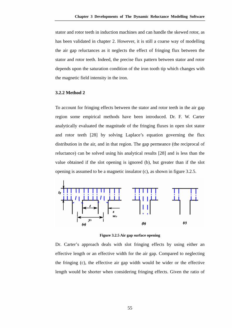
Chapter 3 Developments of The Dynamic Reluctance Modelling Software
55
stator and rotor teeth in induction machines and can handle the skewed rotor, as
has been validated in chapter 2. However, it is still a coarse way of modelling
the air gap reluctances as it neglects the effect of fringing flux between the
stator and rotor teeth. Indeed, the precise flux pattern between stator and rotor
depends upon the saturation condition of the iron tooth tip which changes with
the magnetic field intensity in the iron.
3.2.2 Method 2
To account for fringing effects between the stator and rotor teeth in the air gap
region some empirical methods have been introduced. Dr. F. W. Carter
analytically evaluated the magnitude of the fringing fluxes in open slot stator
and rotor teeth [28] by solving Laplace’s equation governing the flux
distribution in the air, and in that region. The gap permeance (the reciprocal of
reluctance) can be solved using his analytical results [28] and is less than the
value obtained if the slot opening is ignored (b), but greater than if the slot
opening is assumed to be a magnetic insulator (c), as shown in figure 3.2.5.
Figure 3.2.5 Air gap surface opening
Dr. Carter’s approach deals with slot fringing effects by using either an
effective length or an effective width for the air gap. Compared to neglecting
the fringing (c), the effective air gap width would be wider or the effective
length would be shorter when considering fringing effects. Given the ratio of

Chapter 3 Developments of The Dynamic Reluctance Modelling Software
56
slot opening to air gap lengthgls , Carter’s factor for the effective air gap length
can be derived according the Carter’s coefficient curve [25][28].
Carter’s factor gK :
The effective length of the air gap is described by:
ggg lKl =' . (3.2.1)
here Carter’s factor is defined as:
oos
sg wky
yK⋅−
= (3.2.2)
gl′ is the extended (effective) air gap length, gl is the air gap length, sy is the
slot pitch, ow is the slot opening, ok is Carter’s factor which depends upon the
ratio of slot opening to air gap length and is obtained from Carter’s curves. The
effective air gap tooth width modified by Carter’s factor can be derived if the
reluctance remains the same, instead of using the effective length of air gap.
The effective tooth width ew according Carter’s evaluation is:
oose wkyw −= (3.2.3)
The extended air gap length or width formulae given in the previous statement
only hold when one side, either the stator or the rotor is, slotted. If there are
slot openings on both sides of the air gap, then the effective air gap length or
effective width is the product of the air gap length and the product of the two
fringing factors or Carter factors.
222
2
111
121
oos
s
oos
sggg wky
ywky
yKKK⋅−
⋅⋅−
=⋅= (3.2.4)
Where 21, ss yy are the stator and rotor slot pitches respectively, 21, oo ww are
the stator and rotor slot openings and 21, oo kk are the Carter coefficients which
Chapter 3 Developments of The Dynamic Reluctance Modelling Software
57
depend on the ratio of the slot opening to the air gap length and are determined
from Carter’s lookup curve. However, in this case for doubly slotted surfaces
all that are required is to evaluate the effective tooth width of the stator and
rotor independently.
It can be seen that the two sets of formulae that take slot fringing effects into
consideration actually have the same form; the effective air gap length
multiplied by a coefficient which represents the flux passing ratio between the
stator and rotor teeth with respect to the full slot pitch area. The derivation of
this coefficient has been based on rigorous field calculations. Thus, by using
the fringing coefficient or Carter’s factor, fringing fluxes can be taken into
account and this is called Method 2 to model the air gap reluctance and
consequently the machine’s dynamic response can be modelled more
accurately. Unfortunately, in its present form it cannot model the air gap
reluctances whilst fully taking into account any tooth tip saturation effects.
3.2.3 Method 3
In order to take skewed rotors into account, as well as the fringing effects
between the stator and rotor teeth which behave differently for different
saturation levels, and also for coding convenience, air gap reluctance curves
derived from accurate finite element analysis are applied in different small
axial sections of the machine.
Application of FE analysis to the air gap region in induction machines permits
detailed flux distribution patterns to be derived, as shown in figure 3.2.6. A
variety of information is available from this comprehensive and detailed
analysis. However, here only the flux distribution in the air gap region is of
interest. When considering the fringing effects caused by slotting of the stator
and rotor, only the amount of flux leaving or entering the rotor and stator teeth

Chapter 3 Developments of The Dynamic Reluctance Modelling Software
58
surfaces are of interest, in order to represent the fringing effect in terms of an
effective air gap reluctance width. The effective air gap width modelling
method that is obtained by interpolating curves calculated from FEM analysis
is called method 3 in this thesis.
Figure 3.2.6 Overlap curves model for induction machine for method 3
If a single excitation coil carrying a unity current is set on one of the stator
teeth, as shown in figure 3.2.6, then the flux pattern for this specific air gap
geometry can be found by FEM analysis. It shows that, as expected, the
majority of the flux crosses the air gap region to the rotor tooth directly, but
that there is some flux leakage to the adjacent stator teeth. In method 3, the
effective width of air gap reluctances are calculated by deriving the amount of
flux entering the rotor surface, as shown in equation 3.2.6.
Assuming the iron permeability is sufficiently large so that the mmf drop in the
iron can be neglected, the mmf drop only occurs across the air. From an
engineering point of view if the winding current is small (unity current) and the
iron is not saturated, leakage flux to other stator teeth can be neglected as well,
then according to Ohm’s law in a magnetic circuit:
airgaprotormmf ℜ⋅= φ (3.2.5)
where the air gap reluctance is:

Chapter 3 Developments of The Dynamic Reluctance Modelling Software
59
dwl
areaeffective
airgapairgap
0µ=ℜ . (3.2.6)
Using unity motor length in the FEM analysis, gives:
rotorwidtheffective
airgap mmfw
lφµ
=1**0
(3.2.7)
so that the effective air gap reluctance width is given by:
mmfl
w airgaprotorwidtheffective ⋅
⋅=
0µφ
. (3.2.8)
From equation 3.2.8, the effective width of the air gap reluctance for this
specific rotor position and machine geometry can be determined, provided that
the quantity of flux flowing into the rotor surface is known.
By rotating the rotor relative to the stator for a small angle, the air-gap
effective width for a different rotor position can be identified from the FEM
analysis. Repeating this process gives the air gap effective width curve with
respect to the offset between the rotor and stator teeth, as shown in figure 3.2.7
for method 3. This curve can be used in the DRM simulations.
Air Gap Reluctance Curves
-0.002
0
0.002
0.004
0.006
0.008
0.01
0.012
-0.03 -0.02 -0.01 0 0.01 0.02 0.03
Displacements (m)
Rel
ucta
nce
Wid
th (m
)
Method1-Original air gap modelling way
Method3-Air gap modelling curves from FE
Method 2-Air gap modelling method modified byCarter's factor
Figure 3.2.7 Air gap overlap curves for a specific geometry of induction machine with
different methods
Figure 3.2.7 shows the air gap curve comparison for the air gap modelling
Chapter 3 Developments of The Dynamic Reluctance Modelling Software
60
methods, namely method 1, method 2 and method 3. It can be seen that when
the displacement is big, i.e. when the tooth centres are not aligned, air gap
reluctance effective width from method 3 is more than that of method 1
because of the fringing between the stator and rotor tooth pair. However, in the
centre region of the air gap reluctance curve, air gap reluctance width from
method 3 is slightly less than that of method 1. This is due to the leakage flux
between the stator teeth, that some of the flux lines from the excited stator
tooth come into the adjacent stator teeth. The curve for method 2 is wider and
the magnitude is bigger than method 1 and method 3; and in the ‘tail’ of the
curves, curve from method 2 comes closer to that of method 3, indicating a
more accurate modelling of fringing effects. The magnitude of the curve from
method 2 is bigger than the others, because the effective width of the stator and
rotor teeth has been expanded by Carter’s factor thus widening the overlapping
area for the tooth pair when they are aligned.
However, it is necessary to remember, when using this method, that unity
excitation current in the stator coil is used to obtain the effective reluctances
which neglects iron saturation and hence the flux pattern is only valid for
non-saturated stators and rotors. Saturation will alter the flux distribution and
hence the air gap reluctances curves.
As the focus will be on steady state analysis of induction machines, which do
not heavily saturate under normal running conditions, the fact that this
non-saturated air gap reluctance curve is used is acceptable. Even when the
tooth tips are driven into saturation by the large slot leakage flux during the
acceleration phase of a direct on line start simulation, results using this
approach will show only a minor discrepancy between the DRM and FEM
results. However, there will be a significant saving in time and computational
effort thus increasing the computational efficiency.

Chapter 3 Developments of The Dynamic Reluctance Modelling Software
61
For modelling skew, the DRM method described in chapter 2 cuts the rotor
length into several skew sections, to account for the change in flux distribution
along the axis. Rectangular and trapezoidal shape air gap overlap reluctances
are used in a skewed rotor, as seen in figures 2.2.12 to 2.2.14, and the results
shows that the trapezoidal shape air gap reluctances produces less torque ripple
and requires fewer iterations of the solving process. The air gap reluctance
curve in method 3 is obtained from FEM results of a non-skewed rotor
machine. To extend this to a skewed rotor requires that additional techniques be
employed.
As has been described in chapter 2 each of the sections has their own
reluctance mesh and these reluctance meshes are only connected electrically
through the winding coils. Now, each of these sections is further divided into
subsections in order to obtain a more accurate value for the air gap reluctance
effective width. The subsections that are used for calculating effective air gap
width are shown in figure 3.2.8.
Figure 3.2.8 Sub skew sections for effective air gap reluctance calculation in a skewed
rotor induction machine
The effective air gap reluctance width between each subsection of the rotor and
stator is calculated from the effective air gap reluctance curve shown in figure
3.2.7 for this machine geometry, given the offset distance between the stator
tooth centre and the subsection rotor centre. To identify the overall air gap
effective width in this skew section, the average value of the effective widths in

Chapter 3 Developments of The Dynamic Reluctance Modelling Software
62
each subsection is calculated.
∑=
=N
iieffective w
Nw
1
1 (3.2.9)
where, N is the number of sub sections in one skew section, and iw is the
effective air gap reluctance width of the thi sub section. Higher numbers of
subsections provides more accurate skew simulations, noting that the number
of subsections does not affect the simulation speed, since each subsection does
not introduce additional reluctance meshes. Thus, the total number of
reluctances is the same for the machine compared to the use of trapezoidal
shape elements described in chapter 2. A comparison of the results of different
skew modelling methods will be given later in this chapter.
Thus, method 3 accounts for both the tooth fringing effect and the skewed rotor,
and an accurate dynamic induction machine model is now ready for use in
analysis and design.
3.2.4 Comparison of the results for induction machines using Methods 1,
2&3 for modelling the air gap
Three methods for modelling the air gap reluctances in the Dynamic
Reluctance Model of induction machines have been introduced and discussed.
Method 1 correctly accounts for skew and method 2 for tooth fringing effects.
Method 3 can account for both fringing effects and a skewed rotor at the same
time. A comparison of results and discussion will be given in this section.
These simulations are based on a wound induction machine with 48/36
stator/rotor slots, rated power 15kW, rated voltage 415V and skewed one rotor
bar. Machine specifications can be found in Appendix 1. The simulation
scenario is a direct on line start. In order to see the difference between these
methods in coping with skewed rotors, results are given for 1 and 3 skew

Chapter 3 Developments of The Dynamic Reluctance Modelling Software
63
sections in the DRM model. Comparison of these three methods with FEM
analysis is also made to assess the ability to model the fringing effects.
1. Results with a skewed rotor induction machine
The speed versus time curve for an induction machine direct on line start is
shown in figure 3.2.9.
Speed comparison: 1 skew section
0
200
400
600
800
1000
1200
1400
1600
1800
0 0.02 0.04 0.06 0.08 0.1 0.12
Time(s)
Spee
d (r
pm)
M1 M2-width M3
Method 1
Method 2
Method 3
Figure 3.2.9 Comparison of speed curve for a skewed rotor induction machine, simulated
with one skew section
The results show that with only one skew section, a difference is observed for
the speed with the three different methods. Method 1 rises faster than method 3
and so does method 3 to method 2. It is the machine reactance that determines
the induction machine’s rotor acceleration, and the machine reactance is
determined by the leakage reactance and air gap reluctance. In this simulation,
all three methods use the same slot leakage flux model, and the only difference
is the way they model the air gap reluctance, specifically the tooth fringing
effects, which affect the flux passing between stator and rotor tooth surfaces.
The one (method 3), which most correctly accounts for tooth fringing effects
and leakage flux, rises slower than the one that neglects them (method 1). This
is because method 1 underestimates the air gap leakage flux (Zig-Zag flux
[28]). Results from method 2 rise slower than that from method 3 because

Chapter 3 Developments of The Dynamic Reluctance Modelling Software
64
method 2 overestimates air gap leakage flux, which slows down the building
up of the flux field inside the machines thus reducing the torque and speed in
the machine. Both method 2 and method 3 have taken fringing effects into
account thus providing more accurate air gap modelling for the induction
machine.
Speed comparison: 3 skew section
0
200
400
600
800
1000
1200
1400
1600
1800
0 0.02 0.04 0.06 0.08 0.1 0.12
Time (s)
Spee
d (r
pm)
M1 M2-width M3
Method 1
Method 2 Method 3
Figure 3.2.10 Comparison of speed curve for a skewed rotor, simulated with three skew
section
Figure 3.2.10 show that with three skew sections, the three methods agree well.
With the increase of the number of skew sections in the simulation, the
difference between these three methods is further reduced. Essentially, all the
curves are smoother because the cogging torque is greatly reduced.
2. Results with a non-skewed rotor induction machine

Chapter 3 Developments of The Dynamic Reluctance Modelling Software
65
Speed comparison: non-skewed machine
-400
-200
0
200
400
600
800
1000
1200
1400
1600
1800
0 0.02 0.04 0.06 0.08 0.1 0.12
Time (s)
Spee
d (r
pm)
M1 M3 magnet M2-width
Method 1
Method 3FEM
Method 2
Figure 3.2.11 Speed curve comparison with a non-skewed rotor induction machine
Figure 3.2.11 shows that the speed curves from air gap modelling method 2 and
3 agree with the FEM (MagNet) results better than method 1. Because the flux
connection modelled by method 2 and 3 come from rigid field calculations,
thus tooth-fringing effects is accounted for more accurately than for method 1.
Again, it can be seen that method 1 underestimates the air gap leakage flux
between stator and rotor in this specific induction machine simulations, while
method 2 overestimates the air gap leakage flux a little. Also, some cogging
effects due to non-skewed rotor can also be observed in figure 3.2.11. Air gap
modelling method 3 gives the most accurate result compared to FE simulation
results.
3.3 Solving For Conservation of Flux
In the previous section the air gap reluctance modelling method in the DRM
technique has been improved. Additional improvements to the nodal mmf
formulation and equation solving will now be made.
This improvement is provoked by the fact that some flux offset is seen when
calculating the flux linkage in the stator and rotor, as described in [29]. The

Chapter 3 Developments of The Dynamic Reluctance Modelling Software
66
reason for the flux offset is the accumulation of rounding errors when solving
the equations that force the net rate of change of flux entering each node to be
zero. Forcing of the net change in flux to be zero at each node does not
necessarily mean that the net flux flowing into this node is zero as a small and
pseudo-random node mmf offset produced by rounding errors might
accumulate causing the flux offset seen in the solution.
To overcome this problem, the mmf node potential in the equation 2.3.1: is
enforced
( ) 0, 12
1
0=∑
−
=jjj
n
jffφ (3.3.1)
Changing form equations 2.3.1 to equation 3.3.1 does not alter the physical
basis of the modelling process for electrical machines; it is just a numerical
modification to the code which can reduce effect of the rounding on the results.
The equations that define the induction machine electro-magnetic system are
now:
⎥⎥⎥⎥⎥⎥⎥⎥⎥⎥⎥⎥⎥⎥⎥
⎦
⎤
⎢⎢⎢⎢⎢⎢⎢⎢⎢⎢⎢⎢⎢⎢⎢
⎣
⎡
−
−
=
2.3.9equation torque2.3.8equation speed
CphasestatorforequationsloopelectricalBphasestatorforequationsloopelectricalAphasestatorforequationsloopelectrical
1Nlooprotor,cageforequationsloopelectrical
0looprotor,cageforequationsloopelectrical1Nnodeatflux ofonconservati
0nodeatflux ofonconservati
)( bar
node
M
M
xF (3.3.2)
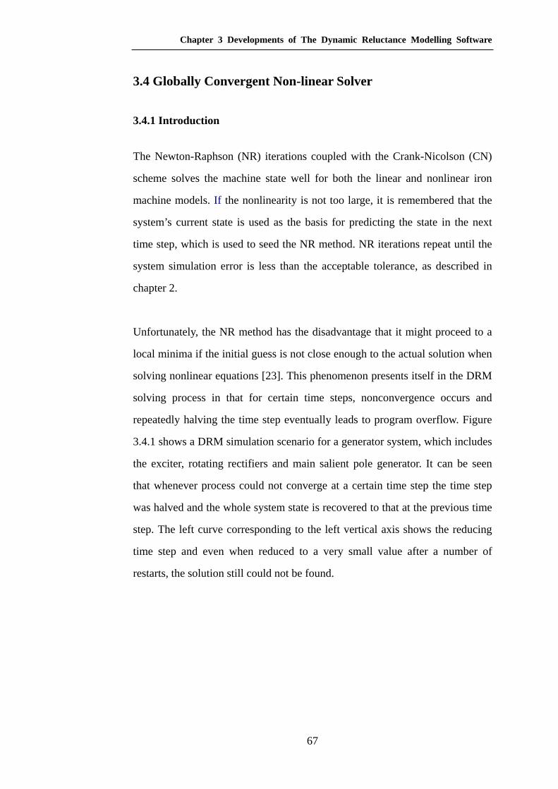
Chapter 3 Developments of The Dynamic Reluctance Modelling Software
67
3.4 Globally Convergent Non-linear Solver
3.4.1 Introduction
The Newton-Raphson (NR) iterations coupled with the Crank-Nicolson (CN)
scheme solves the machine state well for both the linear and nonlinear iron
machine models. If the nonlinearity is not too large, it is remembered that the
system’s current state is used as the basis for predicting the state in the next
time step, which is used to seed the NR method. NR iterations repeat until the
system simulation error is less than the acceptable tolerance, as described in
chapter 2.
Unfortunately, the NR method has the disadvantage that it might proceed to a
local minima if the initial guess is not close enough to the actual solution when
solving nonlinear equations [23]. This phenomenon presents itself in the DRM
solving process in that for certain time steps, nonconvergence occurs and
repeatedly halving the time step eventually leads to program overflow. Figure
3.4.1 shows a DRM simulation scenario for a generator system, which includes
the exciter, rotating rectifiers and main salient pole generator. It can be seen
that whenever process could not converge at a certain time step the time step
was halved and the whole system state is recovered to that at the previous time
step. The left curve corresponding to the left vertical axis shows the reducing
time step and even when reduced to a very small value after a number of
restarts, the solution still could not be found.

Chapter 3 Developments of The Dynamic Reluctance Modelling Software
68
Time step & error graph for brushless generating system
1E-35
1E-33
1E-31
1E-29
1E-27
1E-25
1E-23
1E-21
1E-19
1E-17
1E-15
1E-13
1E-11
1E-09
1E-07
1E-05
0.001
0.1
10
0 20 40 60 80 100 120
Number of restarts
Adj
uste
d tim
e st
ep
0.011100100001000000100000000100000000001E+121E+141E+161E+181E+201E+221E+241E+261E+281E+301E+321E+341E+361E+381E+401E+421E+441E+461E+481E+50
Tot
al sy
stem
err
or
time step system error
Figure 3.4.1 The adjusting of time step and the changing of system error with respect to
the number of restart times in a synchronous machine generating system
The right hand side curve on figure 3.4.1 shows the system error with the
reducing time step. It can be seen that the error becomes larger, which indicates
that the prediction is too far from the system state solution. As the time step
becomes very small numerical rounding dominates the Crank-Nicolson process
and completely undermines the process. This phenomenon is caused by the
significant nonlinearity in this system, in particular due to the nonlinear diode
behaviour. Further detail about the system modelling and its simulation will be
discussed in later chapters. With such a degree of nonlinearity, an initial
prediction that is not close enough to the system solution will cause NR
iterations to fail, as shown in figure 3.4.1.
To solve this, an algorithm that combines the rapid local convergence of
Newton’s method with a globally convergent strategy, which will guarantee
some progress towards the solution at each iteration, is developed [23].
3.4.2 Globally convergent solver for nonlinear systems
As has been described in Chapter 2, the Newton-Raphson step for the set of

Chapter 3 Developments of The Dynamic Reluctance Modelling Software
69
nonlinear system equations
0)( =xF (3.4.1)
is xxx δ+= oldnew (3.4.2)
where FJx ⋅−= −1δ (3.4.3)
J is a Jacobian matrix, and F is the system equation values at a trial
solution oldx . The original Newton-Raphson scheme, as was described in
chapter 2, accepts newx without condition, as long as it is calculated from
equation 3.4.2. However, in the case of system equations with significant
nonlinearity, if the initial guess oldx is not close enough to the system solution,
newx will actually more further away from the system solution than oldx , in this
case the Newton-Raphson algorithm will never converge to the system solution,
and this is a process that one could not control.
If a criterion is used to decide whether to accept the newx or not, the situation
improves. Unacceptable newx , i.e. newx that are further from the solution than oldx ,
can be rejected so that the Newton-Raphson process is more controlled to make
it a globally convergent algorithm.
But, how does one decide whether to accept the Newton step xδ ? A reasonable
strategy is to require that the step decreases FFF ⋅=2 , which is the same
requirement that would be imposed if one were trying to minimise
FF ⋅= 5.0f (3.4.4)
(0.5 is for later convenience) Every solution to equation 3.4.1 minimises the
function f in 3.4.4, but f may also possess local minima that are not
solutions of equation 3.4.1. Thus, simply applying minimum searching
algorithms is not a robust approach.

Chapter 3 Developments of The Dynamic Reluctance Modelling Software
70
To develop a better strategy, note that the Newton step is a descent direction
for f :
0)()( 1 <⋅−=⋅−⋅⋅=⋅∇ − FFFJJFxδf (3.4.5)
Thus the strategy is quite simple: the full Newton step will be tried first,
because once the guess is sufficiently close to the solution quadratic
convergence will be achieved. However, checking the proposed step
reduces f is performed at each iteration. If not, a backtrack along the Newton
direction is undertaken until an acceptable step is found. Because the Newton
step is a descent direction for f , it is guaranteed to find an acceptable step by
backtracking. This method can still occasionally fail by landing on a local
minimum of f , but this is quite rare in practice [23]. The backtrack searching
scheme will be introduced in the following section.
3.4.3 Line search algorithm for globally convergent solving scheme
The line search (backtracking search) algorithm is to search for the proper
Newton-Raphson step that reduces the system error in function 3.4.4
sufficiently along the Newton direction.
When the initial guess is close enough to the minimum of f , taking the full
Newton step would help one to find the system solution with quadratic
convergence. When it is not close enough to the minimum of f , the move
might be too far for the full Newton step xp δ= to decrease the function as the
quadratic approximation is not valid here. So the goal is to move to a new
point newx along the direction of the Newton stepp , but not necessarily all the
way:
Chapter 3 Developments of The Dynamic Reluctance Modelling Software
71
pxx λ+= oldnew (3.4.6)
where,
10 << λ . (3.2.7)
The aim is to find λ so that )( px λ+oldf has decreased sufficiently.
If )( newf x does not meet our acceptance criteria, we backtrack along the
Newton direction, trying a smaller value ofλ , until a suitable point is found.
Since the Newton direction is a descent direction, it is guaranteed to
decrease f for sufficiently smallλ .
But, how is it possible to tell if )( px λ+oldf has decreased sufficiently? The
suggested criteria for accepting a step, by W. H. Press [23], to require that the
average rate of decrease of f is at least some fractionα of the initial rate of
decrease p⋅∇f :
)()()( oldnewoldnew fff xxxx −⋅∇+≤ α (3.2.8)
Here the parameter α satisfies 10 <<α . Then, theλ value in each iteration
needs to be found.
A strategy for a practical backtracking routine is as follows:
Define:
)()( px λλ +≡ oldfg (3.2.9)
such that:
p⋅∇=′ fg )(λ (3.2.10)
Here, the algorithm begins with a step multiplier of 1 (full Newton step) and
then backtracks until an acceptable reduction in the performance is obtained.
On the first step the value of performance at the current point )0(g is used, and
a step multiplier value of )1(g . Use of the value of the derivative of the
Chapter 3 Developments of The Dynamic Reluctance Modelling Software
72
performance at the current point )0(g′ is also made to obtain a quadratic
approximation to the performance function along the search direction,
hence )(λg can be modelled as a quadratic:
)0()0()]0()0()1([)( 2 gggggg +′+′−−≈ λλλ , (3.2.11)
then the minimum of the quadratic is found as:
)]0()0()1([2)0(
gggg
′−−′
−=λ . (3.2.12)
This minimum of the quadratic approximation becomes a trial point for where
the function )( px λ+oldf has its minimum value, and the performance at this
point is tested. If newf is not sufficiently reduced, on the second and
subsequent backtracks, a cubic model of )(λg is obtained and the minimum
of the cubic interpolation becomes the new trial point. The cubic model of
)(λg is:
)0()0()( 23 ggbag +′++= λλλλ (3.2.13)
where,
⎥⎦
⎤⎢⎣
⎡−′−−′−
⋅⎥⎥⎥
⎦
⎤
⎢⎢⎢
⎣
⎡
−
−
−=⎥
⎦
⎤⎢⎣
⎡)0()0()()0()0()(
111
22
11
221
122
22
12
21 gggggg
ba
λλλλ
λλ
λλ
λλλλ
(3.2.14)
The minimum of this cubic occurs at:
agabb
3)0(32 ′−+−
=λ (3.2.15)
This process is continued until sufficient reduction in the performance error is
obtained. The line search algorithm flow chart is shown in figure 3.4.2.
Figure 3.4.2 shows the flow chart of the line search scheme, which is entered
after the BiCGSTAB solver solves for the full Newton step. As described above
the aim of this line search function is to find a proper step that minimises the
Chapter 3 Developments of The Dynamic Reluctance Modelling Software
73
error function f . The slope is calculated after the full Newton step is made and
then a scheme for detecting small changes is applied to avoid too close a
distance between newx and oldx . Subsequently, parameterλ is set to be 1 (a full
Newton step) when the algorithm starts and the error function value f at that
time is evaluated. If it is decreased sufficiently, as defined by equation 3.2.8,
the line search ends; if not, the line search function will model the
function )(λg by a quadratic in the first searching step, as described in equation
3.2.11; and by a cubic in the subsequent backtracks, as described in equation
3.2.13. Theλ value when this minima of )(λg occurring is derived from the
cubic and quadratic models. The error function value is evaluated again to see
if it is decreased sufficiently. This line search iteration process will continue
until sufficient decrease in the error function f is achieved.

Chapter 3 Developments of The Dynamic Reluctance Modelling Software
74
start
Calculate slope=g[i]*p[i]
If slope<0, display roundofferrors
Guard against too small avalue of lamda
Iteration start
Calculate alamin
Xnew=Xold+ alam*p[i]
Evaluate function value
Alam<alamin?
*f<fold+ala*slopesufficient function
decrease?
Alam=1?First step?
Full NR step,quadratic minima
g e t t e n t a t i v eoptimum point
Subsequentbacktracks; cubic
minima
Next iteration
X=xold, return
Convergence on delX
Return;
Display sufficient functiondecrease
Figure 3.4.2 Flow chart of line search backtrack algorithm
3.4.4 Global convergent technique flow chart
After modification with the line search backtracking algorithm, the
Newton-Raphson method provides a nonlinear multi-dimensional solving
technique with global convergence. Figure 3.4.3 shows the core routine of this
global convergent solver, the pre- and post-processor are the same as described
previously at chapter 2.

Chapter 3 Developments of The Dynamic Reluctance Modelling Software
75
Each time steploop
Time=time+dt
Obtain drivingvoltages for stator
Newton-Raphsonloop
Calculate system equations?error function andJacobian matrix
Initial solutionconverge?
Linear solver- preconditioned ConjugateGradient solver (BiCGTAB)
Calculate slope g[i]
Line search backtrack function fornewton step
Functiondecrease
sufficiently?
Iteration<MAXITER?
Clear linearsolver object
Write results to file
Solving process
Yes
No
Yes
No
A
BC
Create air gap elements for this specificrotor position
Yes
No
Figure 3.4.3 Solving process of a globally convergent Newton-Raphson solver

Chapter 3 Developments of The Dynamic Reluctance Modelling Software
76
Number of modified NR iteration
0
5
10
15
20
25
30
1 2 3 4 5 6 7 8 9 10 11 12 13 14 15 16 17 18 19 20 21 22 23 24 25 26 27 28 29 30 31 32 33 34 35 36 37 38 39 40 41 42 43
Number of time step
Num
ber o
f NR
iter
atio
n
Number of modified NR iteration Figure 3.4.4 Number of NR iteration for globally convergent nonlinear solver vs. time
step
Figure 3.4.4 shows how a system with significant nonlinearity (rectifier), is
solved with the modified globally convergent NR solver. It solves the same
systems as the original NR solver with which nonconvergence happens, as
shown in figure 3.4.1. These two simulations use the same simulation
parameters, i.e. time step, threshold and tolerance etc. and it can be seen that
this nonlinear system is solved properly with the new NR solver.
The core solving technique has been modified to use an algorithm which can
deal with nonlinear, sparse, first order differential equations and is globally
convergent. The DRM now provides a powerful tool for systems with
significant nonlinearities and other complexities, such as control loops. This
solver will be utilised throughout the simulations in this thesis.
3.5 Detailed Slot Leakage Model for Induction Machine
In section 2.2.2, a typical induction machine reluctance mesh is given for the
stator and rotor, including for the air gap region. It is quite a coarse mesh, and
becomes inadequate when one wants to accurately assess a machine’s transient
behaviour, such as the direct on line start of an induction machine.

Chapter 3 Developments of The Dynamic Reluctance Modelling Software
77
In starting conditions, the winding currents in an induction machine are large
and thus leakage fluxes between the stator and rotor slots are large as well. The
leakage and working fluxes in machines are defined by Steven [30]:
‘The total flux in a machine has components, viz:
(a) Working flux, which links both the stator and rotor windings;
(b) Leakage flux, which links one winding only and generally, gives rise in an
equivalent circuit interpretation to a component leakage reactance. The
leakage inductance is an important parameter in calculations concerned
with analysis of a.c. machines. In d.c. machines, it is of importance in
relation to commutation, and in field estimation.’
These leakage fluxes play an important part in machine transients. In order to
model the induction machine more accurately, as well as to improve the
accuracy of other machine transient models, such as the short circuit condition
in generators, reluctances that represent leakage fluxes have to be added to the
dynamic reluctance mesh model. Only slot leakage inductances in electrical
machines are considered here, although end winding leakage inductance could
also be added as lumped inductors in the stator and rotor electrical circuit.
In the typical reluctance mesh model for an induction machine given in chapter
2, shown in figure 2.2.6, there is reluctance across the air gap region
representing the slot leakage flux. However, there is also leakage flux existing
in the space occupied by the winding, as shown in figure 3.5.1 named the
winding region. To model the induction machine behaviour accurately, the slot
leakage reluctance representing the winding region leakage flux has to be
added into the induction machine reluctance mesh. This section will discuss
how this reluctance is calculated.

Chapter 3 Developments of The Dynamic Reluctance Modelling Software
78
Figure 3.5.1 Air gap reluctances between stator and rotor teeth
When the windings carry current, they set up a slot-leakage flux pattern with a
complex shape [28], as shown in figure 3.5.2. If there is a relative large space
below the bottom conductor and its width is substantially less than that of the
slot, then the field pattern is that shown in (a).
Figure 3.5.2 Slot leakage flux pattern in parallel slots, accommodating one rectangular
conductor
However, the proportions are more usually those of (b), in which the field
pattern is very nearly in the form of straight lines across the slot. This pattern is
readily analysed, and is adequate for steady currents or those of low frequency,
but fails (unless the conductors are subdivided and transposed) for frequencies
approaching normal industrial supply values. The straight-line model is
adopted here as it is sufficient for our industrial purposes.
For different slot shapes, different ways of calculating the leakage reluctances
are adopted. Two commonly used induction machine slot shapes will be

Chapter 3 Developments of The Dynamic Reluctance Modelling Software
79
discussed in the following section.
3.5.1 Semi-closed rectangular slot
This semi-closed rectangular slot shape is usually used for induction machine
stators. Considering the dimensions in figure 3.5.3, the permeance coefficient
per unit axial length is the ratio (area/length) of the air path considered. The air
gap regions above the conductors are 0
3
wh for the lip and
0
22ww
h
s +for the
wedge portion immediately above the conductor.
Figure 3.5.3 Semi-closed slot profiles
The slot region occupied by the conductor has to be treated differently. All the
leakage flux above the conductor links the conduction wholly, but the flux at a
height x, shown in figure 3.5.4, only links the lower part of the conductor and
contributes only partial linkage. Thus, such flux has a lower density as only the
fraction (1hx ) conductor, uniformly distributed, and is linked by the point where
is considered, as shown by x in figure 3.5.4.

Chapter 3 Developments of The Dynamic Reluctance Modelling Software
80
Figure 3.5.4 Schematic plot of slot leakage reluctance calculation
Consider the flux path loop shown in figure 3.5.4 whose top is x above the
bottom of the conductor, the mmf enclosed is:
)(1
Nihxmmf = (3.5.1)
so that the flux in the elemental path dx is:
dxhx
wNi
dxw
mmfmmfdssx
⋅⎟⎟⎠
⎞⎜⎜⎝
⎛⋅=
⋅⋅
=ℜ
=1
0
0
)(
1
µ
µ
φ (3.5.2)
which links the proportion 1hx of the conductor. Therefore, the flux linking this
part of elemental dx is:
dxhx
wNi
hxNd
ss ⋅⎟⎟
⎠
⎞⎜⎜⎝
⎛⋅⎥
⎦
⎤⎢⎣
⎡⎟⎟⎠
⎞⎜⎜⎝
⎛=
10
1
µλ (3.5.3)
and hence the total coil-side flux linkage is:
s
h
sc w
hiNdxxhw
iN3
1 120
2
12
0
2
0
1
µµλ =⋅⎟⎠⎞
⎜⎝⎛= ∫ (3.5.4)
from which the reluctances of the air gap reluctances representing leakage flux
are derived as:

Chapter 3 Developments of The Dynamic Reluctance Modelling Software
81
⎟⎠⎞
⎜⎝⎛
==⋅
==ℜ
31
0
2
hwiNNmmfmmf s
ccc
µλλφ . (3.5.5)
It can be seen that by considering slot leakage flux, the width of the slot
leakage reluctance is actually one third of the slot depth. This leakage
reluctance can be used in the DRM to account for slot leakage fluxes in
semi-closed shape induction machine modelling.
Instead of using one discrete reluctance element representing the slot leakage
effects between stator and rotor slots in induction machines, two reluctances
can also be used, in a more complicated reluctance mesh. Further discussion
regarding the reluctance mesh topology will be presented in chapter 7.
3.5.2 Round slots
Round slot shapes are usually used in cage rotor induction machines. The cage
bars on the rotor are round bars, deep bars, or double bars. The machine under
investigation for time being has round slots as shown in figure 3.5.5.
Figure 3.5.5 Round slot profiles
Assume that the flux crosses the slot in straight lines; the slot leakage
reluctance for this type of slot is independent of the slot diameter. An empirical
formula suggested for the leakage reluctance is [28]:

Chapter 3 Developments of The Dynamic Reluctance Modelling Software
82
( )100
0
66.0 hww
c +=ℜµ (3.5.3)
i.e., the width of the slot reluctance reduced by ( )1066.0 hw + . Neglecting the
slot opening the equivalent reluctance cℜ is:
( )66.01
0µ=ℜc . (3.5.4)
Employing the slot leakage reluctances to both the stator and rotor sides in the
dynamic reluctance mesh method as shown in figure 3.5.6, provides a more
accurate reluctance mesh for induction machines.
Figure 3.5.6 Modified dynamic reluctance mesh for induction machine which accounts for
slot leakage flux
It is observed that the reluctances in light colour between the stator slots and
rotor slots represent the slot leakage flux calculated from the previous method.
With the modification of these reluctances to the reluctance mesh of induction
machines, the simulation of the direct on line start of an non-skewed rotor
induction machine becomes even closer to the FEM results, as shown in figure
3.5.7.

Chapter 3 Developments of The Dynamic Reluctance Modelling Software
83
Induction machine, DOL start,speed comparison
-200
0
200
400
600
800
1000
1200
1400
1600
1800
0 0.01 0.02 0.03 0.04 0.05 0.06 0.07 0.08 0.09 0.1
Time(s)
Spee
d (r
pm)
without slot leakage reluctancewith slot leakage reluctance
FEM
Figure 3.5.7 Induction machine direct on line start speed curve, with and without slot
leakage reluctance modelled, in comparison to FEM results
3.6 Conclusion
This chapter describes the notable improvements made to the original Dynamic
Reluctance Mesh modelling software, which makes the DRM simulations more
accurate and stable.
First, modifications of the air gap reluctance models are introduced and results
are given in comparison with FEM results which show the improvement in
modelling of induction machines.
Modifications were also made for solving the system state equations. Solving
for the conservation of flux in each node is applied rather than solving for the
rate of change of flux, in order to eliminate the residual flux caused by
computational round off errors.
In order to overcome the nonconverge problems, which happen when solving
systems with significant nonlinearity, a modified globally convergent

Chapter 3 Developments of The Dynamic Reluctance Modelling Software
84
Newton-Raphson nonlinear solver is applied, which incorporates line searching
schemes to identify a proper Newton step.
Also, simulating an induction machine direct online start, the modelling of slot
leakage inductance is known to be important. The reluctances that represent the
leakage flux between the stator and rotor slots have been added to the
reluctance mesh for induction machines previously described in chapter 2. The
results show that these slot leakage reluctances improve transient performance
modelling in comparison with FEM results.
With all these modifications and improvements made to the DRM simulations,
other machines with more complicated geometries can be modelled. These
include salient pole synchronous machines with nonlinear circuit components.
Complex control schemes can also be incorporated in the simulation.

Chapter 4 Modelling and Simulating Salient Pole Synchronous generators
85
CHAPTER 4 MODELLING AND SIMULATING
SALIENT POLE SYNCHRONOUS GENERATORS
4.1 Introduction
Three phase synchronous generators are the primary source of all the electric
energy we consume today. Some of these machines are the largest energy
converters in the world with ratings of up to 1500 MW. There are relatively
small numbers of very large generators which include turbo-generators, driven
by steam turbines and hydro generators, driven by water turbines. The majority
of industrial generators have ratings up to 1000 kVA, and are driven by gas
turbines and diesel engines. They are used for small power systems e.g. oil
platforms, ships and remote industrial sites as well as for combined heat and
power and standby cases, for such as transportation systems or hospital backup
power supplies.
Turbo-generators usually have a forged, cylindrical rotor to reduce the effect of
centrifugal force on the rotor structure due to their low pole number and high
rotational speed together with their relatively large diameter resulting from the
high power rating. Large gas turbine generators also follow this basic design
form. However, for the relatively low speed, or low power prime movers, rotor
specifications usually define a salient-pole structure. This covers hydro
generators and small rating industrial generators driven by diesel engines.
After a long period of stability of the development in electrical power systems
in the UK, there has recently been increasing development resulting in greater
complexity and increasing scale of the power system. Local generation in the
UK means that it becomes more and more important to simulate power system

Chapter 4 Modelling and Simulating Salient Pole Synchronous generators
86
behaviour under different circumstances, such as fault conditions, in order to
make the whole power system more efficient and stable and to develop correct
protection strategies. Among the simulation models required of the power
system components, one key model is the electric generator. From a power
system standpoint, this may not need to be too complex. However, the
generator manufacturer’s standpoint is different.
Small power systems are increasingly common and pose problems in terms of
reliable operation. The ability to clear faults effectively without the generator
voltage sagging to the point where discrimination is compromised is a key
requirement. Additionally, it is not uncommon for small systems to have large,
key pieces of motor driven plant which must be able to be started even when
not all of the paralleled generators are available. Such cases impose high
transient load currents though the power required will be within the generator’s
capacity. These systems need to be modelled carefully from the generator
manufacturer’s point of view to ensure high customer satisfaction.
Thus, for both large, complex and for small power systems the generator
manufacturer requires a detailed model of his product which can facilitate the
development of machines that are both profitable to make and reliable in
operation. The key features required for this situation are the ability to model,
in detail, the excitation, the generation and the voltage regulation control
systems. The model should also be capable of incorporating dynamic machine
loads and simple power system loads. Additionally, the model must be
sufficiently computationally efficient so that several “what if” scenarios or
different design changes can be examined in a reasonable time scale.
Various models of small salient pole generators have been proposed [2][31],
and the Dynamic Reluctance Mesh model is one of these. The advantage of the
DRM approach is that it includes an essentially 2D model of saturation and

Chapter 4 Modelling and Simulating Salient Pole Synchronous generators
87
slotting in the machine. This can be extended to pseudo 3D to incorporate skew.
However, it is not a very difficult step to extend the model to include the
exciter, the rotating rectifier and the automatic voltage regulator (AVR). This
can be difficult and very computationally intensive if attempted with Finite
Element software, though more detailed modelling of the electromagnetic
operation of the machine would be expected. Simple dynamic modelling based
on Park’s approach [32] and generalised machine theory is much more rapid
than either of the magnetic-field based approaches but is much less able to
model the detail of saturation and slotting in the machine.
This chapter is concerned purely with modelling the generator itself and not
with the exciter and AVR. Initially the standard generalised machine model
suitable for Matlab based analysis will be developed both to introduce the
transient coupled circuit approach and to show the simplifications inherent in
this approach. The magnetic field based models, FEM and DRM, will then be
introduced. The first objective of the chapter is to show that a suitable DRM
model gives excellent results for predicting machine performance. The second
objective is to define the degree of complexity of the DRM model required to
give that excellent performance. The third objective is to show that the DRM
can provide excellent, though less detailed, results much more rapidly than the
equivalent FEM approach. To do this, results for open circuit and short circuit
transients predicted by both FEM and DRM approaches will be compared, not
only with respect to each other but also with practical results obtained on an
experimental machine. A typical industrial salient pole generator is used as an
example, whose basic specifications are three phase, four poles, four hundred
volts, fifty Hz, 68kW. The stator has a conventional winding. The field winding
on the rotor is fed via slip rings. Full details of this machine are presented in
Appendix 1.
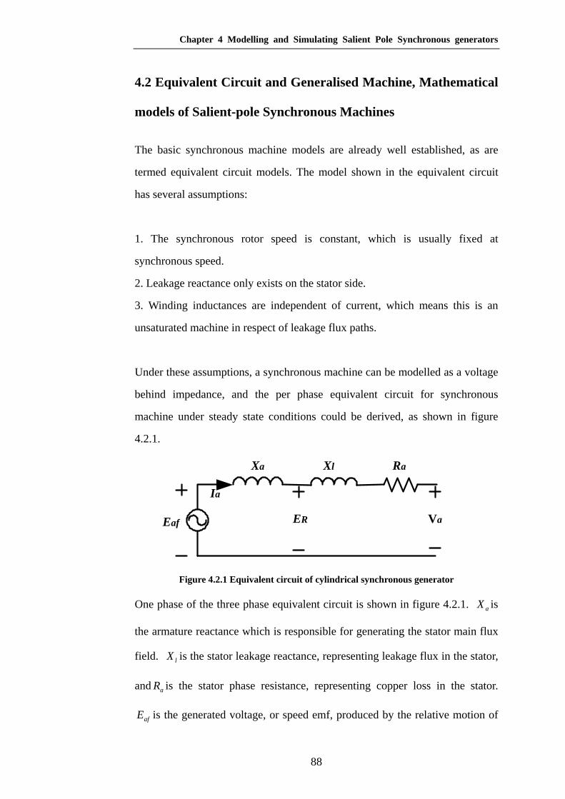
Chapter 4 Modelling and Simulating Salient Pole Synchronous generators
88
4.2 Equivalent Circuit and Generalised Machine, Mathematical
models of Salient-pole Synchronous Machines
The basic synchronous machine models are already well established, as are
termed equivalent circuit models. The model shown in the equivalent circuit
has several assumptions:
1. The synchronous rotor speed is constant, which is usually fixed at
synchronous speed.
2. Leakage reactance only exists on the stator side.
3. Winding inductances are independent of current, which means this is an
unsaturated machine in respect of leakage flux paths.
Under these assumptions, a synchronous machine can be modelled as a voltage
behind impedance, and the per phase equivalent circuit for synchronous
machine under steady state conditions could be derived, as shown in figure
4.2.1.
Ia
Xa Xl Ra
Eaf ER Va
Figure 4.2.1 Equivalent circuit of cylindrical synchronous generator
One phase of the three phase equivalent circuit is shown in figure 4.2.1. aX is
the armature reactance which is responsible for generating the stator main flux
field. lX is the stator leakage reactance, representing leakage flux in the stator,
and aR is the stator phase resistance, representing copper loss in the stator.
afE is the generated voltage, or speed emf, produced by the relative motion of

Chapter 4 Modelling and Simulating Salient Pole Synchronous generators
89
stator and rotor main flux fφ . RE is the voltage generated by resultant air gap
flux Rφ . Part of the input mechanical energy is stored as magnetic energy
represented by aX , and aV is the phase terminal voltage, i.e. output voltage of
phase A of the generator.
Figure 4.2.2 shows the phasor diagram of the cylindrical synchronous
generator in a steady state, over-excited condition.
φ
Direct Axis
Quadrature Axis
IaVa
IaRa
ER
jIaXl
jIaXa
δ
Eaf
FR
Fa
Ff
Figure 4.2.2 Phase diagram of cylindrical synchronous generator in steady state under
excited
The angleδ is the load angle, which is the angle between the flux produced by
the rotor and the resultant flux. Figure 4.2.2 shows quite clearly how the
machine operates in steady state, for a generator afE leads aV . In general, for a
lagging power factor the machine is over excited and for a leading power factor
it is under excited.

Chapter 4 Modelling and Simulating Salient Pole Synchronous generators
90
The three phase electrical equations for simulating a simplified cylindrical
rotor machine in the steady state condition is:
aaasaaaf RIIjXVE ++= (4.2.1)
bbbsbbbf RIIjXVE ++= (4.2.2)
cccscccf RIIjXVE ++= (4.2.3)
where lasa XXX += , lbsb XXX += , lcsc XXX += individually.
The salient pole rotor synchronous generator is different from the machine with
cylindrical rotor in that there is a preferred magnetising direction in the salient
rotor machine because of the non-uniform air gap. Thus, for analytical
convenience, currents, voltages and fluxes are resolved in the d and q axis,
where the d axis is the preferred flux magnetising direction, while the q is the
axis perpendicular to the d axis electrically.
In salient pole generator analysis, it is more convenient to transform the
currents and voltages from the stationary ABC frame to the rotating dq frame,
which rotates synchronously with the rotor normally at synchronous speed.
Park’s transformation [32] is used when transforming from the stationary stator
frame to the rotor frame, as shown in Equation 4.2.4. Assume:
abcdq xPx ⋅=0
where x denotes the variables in each reference frame, such as currents,
voltages etc.. and P is Park’s transformation matrix:
⎥⎥⎥⎥⎥
⎦
⎤
⎢⎢⎢⎢⎢
⎣
⎡
+−+−⋅=
)3/2sin()3/2sin()sin()3/2cos()3/2cos(cos
21
21
21
32
πθπθθπθπθθP (4.2.4)
After transformation to the dq frame, the equations describing the salient-pole

Chapter 4 Modelling and Simulating Salient Pole Synchronous generators
91
synchronous generator in steady state are:
ddqaqf IjXIRVE +=−
qqdad IjXIRV +=− (4.2.5)
where mdlsd XXX += , mqlsq XXX += , the direct- and quadrature- axis
synchronous reactances, according to d-axis and q-axis theory, and lsX is stator
d and q axis leakage reactance, and dX and qX are magnetising reactance for
d and q axis.
The transformed phasor diagram for the synchronous generator is shown in
figure 4.2.3, when the salient pole generator running in the steady state
condition, over excited.
φ
Direct Axis
Quadrature Axis
Ia
Va
IaRa
δ
Ef
FR
Ff
Id
Iq
jIdXd
jIqXq
Fq
Fd
Vq
Vd
Figure 4.2.3 Phase diagram for salient-pole synchronous generator
The transformed dq model has been mentioned in previous context, however,

Chapter 4 Modelling and Simulating Salient Pole Synchronous generators
92
in a typical salient pole synchronous machine, there are damper windings
positioned on the surface of the salient pole, and these need to be considered in
the generator’s dq mathematical model as well. Normally these are also
resolved onto d and q axes for the convenience of analysis. A two pole,
three-phase wye-connected salient pole synchronous machine with damper
windings is shown in figure 4.2.4.
Figure 4.2.4 Two pole, three phase, salient pole synchronous machine windings
arrangements
A , B andC are in the three phase stationary frame, d- and q- are in the two
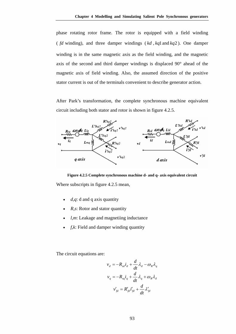
Chapter 4 Modelling and Simulating Salient Pole Synchronous generators
93
phase rotating rotor frame. The rotor is equipped with a field winding
( fd winding), and three damper windings ( kd , 1kq and 2kq ). One damper
winding is in the same magnetic axis as the field winding, and the magnetic
axis of the second and third damper windings is displaced 90° ahead of the
magnetic axis of field winding. Also, the assumed direction of the positive
stator current is out of the terminals convenient to describe generator action.
After Park’s transformation, the complete synchronous machine equivalent
circuit including both stator and rotor is shown in figure 4.2.5.
Figure 4.2.5 Complete synchronous machine d- and q- axis equivalent circuit
Where subscripts in figure 4.2.5 mean,
• d,q: d and q axis quantity
• R,s: Rotor and stator quantity
• l,m: Leakage and magnetiing inductance
• f,k: Field and damper winding quantity
The circuit equations are:
qRddsdd dtdiRv λωλ −+−=
dRqqsqq dtdiRv λωλ ++−=
fdfdfdfd dtdiRv λ′+′′=′

Chapter 4 Modelling and Simulating Salient Pole Synchronous generators
94
kdkdkdkd dtdiRv λ′+′′=′
1111 kqkqkqkq dtdiRv λ′+′′=′
2222 kqkqkqkq dtdiRv λ′+′′=′
where:
)( kdfdmdddd iiLiL ′+′+−=λ
)( 21 kqkqmqqqq iiLiL ′+′+−=λ
)( kddmdfdfdfd iiLiL ′+−+′′=′λ
)( fddmdkdkdkd iiLiL ′+−+′′=′λ
)( 2111 kqqmqkqkqkq iiLiL ′+−+′′=′λ
)( 1222 kqqmqkqkqkq iiLiL ′+−+′′=′λ
and,
mqlqq LLL +=
mdldd LLL +=
mqlkqkq LLL +′=′ 11
mqlkqkq LLL +′=′ 22
mdlfdfd LLL +′=′
mdlkdkd LLL +′=′ .
With these equations derived, the synchronous generator machine state could
be solved with commercial simulating software, such as Matlab. Matlab
provide a machine library, which has some synchronous machine models with
different units and parameter inputs.
As for the other complicated characteristics such as saturation and transient
state, there are various models accounting for these.

Chapter 4 Modelling and Simulating Salient Pole Synchronous generators
95
For simulating the transient and sub-transient conditions, Arrillaga [33] and
Saccomanno [31] mentioned the salient-pole synchronous machine
mathematical model under transient and sub-transient conditions. Additional
fictitious voltages dE′ and qE′ are added which represent the flux linkages due
to the ‘inertia’ of flux change in the rotor winding during transient conditions.
Thus, two additional rotor circuits (equations) are added, one of which acts
magnetically along the direct axis, and the other along the quadrature axis. For
sub-transient conditions, voltages dE ′′ and qE ′′ , and another two voltage equations
are added for the same reason.
Saturation is a part of synchronous machine modelling but there is still
uncertainty as to what is the best method of simulation. The degree of
saturation is not the same throughout the machine because the flux density
varies for different parts of the machine due to the design of the geometry of
the machine. The saturation in the direct and quadrature axes are different.
For the mathematical synchronous machine model, saturation may be taken
into account by modifying the value of the reactance used in representing the
machine [33], including both the d and q reactances for the cylindrical machine
and the salient-pole machine. Various methods have been adopted to account
for saturation in both modification of the technique and in the representation of
the saturation characteristic of the machine, such as the classical saturation
model, salient-pole saturation model, which modify the synchronous reactances,
the simple saturation representation, and the Potier reactance [33]. Saccomanno
[31] considered saturation in the stator side and the rotor side separately and
then combined the effects.
Overall, the models developed so far are simple. Park’s transformation assumes
sinusoidal flux distribution and winding distributions and so neglects slotting

Chapter 4 Modelling and Simulating Salient Pole Synchronous generators
96
and phase belt harmonics [32]. Saturation is included in various ways but
rarely with any detail since leakage flux paths are not separately identified and
so the dependence of leakage reactances on winding current levels is
imperfectly modelled, or ignored. Main flux saturation is treated in some
methods with more detail yet secondary effects of armature reaction in terms of
cross saturation are not well modelled and more normally neglected [32]. Not
least of the problems with this method is the need for machine inductance
values as well as speed emf constants and saturation data if the model is able to
cope with it. This data can be determined experimentally for existing machines
but if the approach is used to analyse new designs there is a consequent need
for an additional machine design program to determine these values. It is very
much apparent that this type of model is aimed more at systems analysis than at
detailed machine behaviour analysis. However, the approach is very widely
used.
4.3 Finite Element Models of Salient Pole Synchronous
Machines
The finite element method (FEM) is a widely used field calculation method,
which can be used in many engineering fields, including mechanical, material,
structural, thermal, fluid, and electromagnetic field calculations. It can supply
very detailed and accurate field information to meet user requirements, thus
quite often, it is the benchmark of many engineering numerical simulation
results. However, although generally speaking, the FE method is accurate, the
accuracy and reliability depends on the discretising of the intended calculation
objects and the polynomial order for interpolation. Results would be different
using different solving parameters and discretising method, and interpolation
techniques.
Due to the advantage of the FE method, it has been an effective method of

Chapter 4 Modelling and Simulating Salient Pole Synchronous generators
97
investigating complicated electrical apparatus, such as electrical machines,
which includes detailed flux field distribution, inductances calculations
although the calculation time may be vast. There are also commercial software
packages developed for each kind of specific application, such as MagNetTM
for the calculation of electrical machines or ANSOFTTM for combined
calculation of structure analysis, mechanical analysis etc.
One type of salient pole synchronous generator was modelled with commercial
FEM software package. The machine rating was 68kw, 4 poles with 0.8 power
factor. By using a time stepping method, the transients of the generator in the
open circuit condition were calculated, where the field excitation voltage is
added on the rotor circuit terminal, and the rotor is driven by prime mover at a
constant synchronous speed. The generated stator terminal voltage and field
current, and also the air gap flux density distribution are examined. A
comparison of results between FEM and DRM is given in the flowing
discussion.
Figure 4.3.1 shows the solution mesh from FE calculations at a specific time
step. Automatic mesh adaption method is used at each time step calculation, so
that the program will optimise the topology of the mesh in preparation for the
next time step for a more accurate solution.

Chapter 4 Modelling and Simulating Salient Pole Synchronous generators
98
Figure 4.3.1 Solution mesh of the salient-pole synchronous machine in a specific time step
@100ms
As can be seen from the figure, the meshed elements close to the air gap and in
the stator slot and rotor surface region are denser than the others. This is due to
the air gap geometry, which is more irregular compared with that of an
induction machine, and is more important from the machine modelling point of
view, because it is the air gap that carries the flux field between stator and rotor.
In the solution mesh, there are 72,076 triangles in total.
The machine stator winding is a double layer concentric winding with a coil
pitch of eight, parallel circuits, forty-eight slots and five number of turns. The
winding was formed in each phase from four coils. As normal in four wire
generators, to eliminate the harmful third harmonic, the stator three phases are
star connected with a 120 degree coil pitch. The circuit in figure 4.3.2 shows
the simulated winding coil connections in the FEM model of this type of
generator. It simulates an open circuit condition, with a very large resistance
value connected to the stator terminals to simulate an open circuit condition
numerically. Rated value d.c. voltage source is applied to the rotor side as the
excitation. All the damper bar windings are connected together as for the rotor

Chapter 4 Modelling and Simulating Salient Pole Synchronous generators
99
of a cage induction machine.
Figure4.3.2 Electrical circuit connection model of a type of salient-pole synchronous
generator simulated in FEM software
For the nonlinear iron material, Losil 800 as stated in the generator datasheet,
is selected in the FE model from the material database in the finite element
software. Thus, the b-h curve is used in simulation to represent the nonlinear
relationship between the field intensity and the actual flux density in the
material.
For the rotating, transient magnetic field calculation, it normally takes days or
weeks to achieve the results, depending on the problem scale and accuracy
requirements. In the simulations in this chapter, a time step of 1ms was used,
simulation time was 300ms, adaptive h-adaption was used for the meshing
process, CG tolerance was 0.001 and Newton tolerance was 0.01. The total
simulation time for the full FE model was 576 hours. While for a DRM
simulation, for a time stepping method with time step to be 0.00001, solving

Chapter 4 Modelling and Simulating Salient Pole Synchronous generators
100
tolerance to be 10e-8, the solution time for 1s would be taken for 10 hours. The
simulation time comparison between FE and DEM is shown in table 4.3.1.
Time step Newton tolerance
Simulation time
Time take for simulations
Calculation time for each time step
FEM 0.001s 0.01 0.3s 576 hours 0.52 hour/step
DRM 10e-5s 10e-8 1s 10 hours 1e-4 hour/step
Table 4.3.1 Simulation time comparison between FEM and DRM
Figure 4.3.3 shows the detailed flux function distribution result in one specific
time step for the whole machine.
Figure 4.3.3 Flux function distribution in a salient-pole synchronous machine calculated
by FEM software, results taken @100ms
Figure 4.3.4 to figure 4.3.6 show the results for the rate of growth of field
current following initial switch on as calculated from FEM software for this
type of salient pole synchronous machine.

Chapter 4 Modelling and Simulating Salient Pole Synchronous generators
101
Field Current
0
0.5
1
1.5
2
2.5
3
3.5
4
0 0.05 0.1 0.15 0.2 0.25 0.3
time(s)
Rot
or c
urre
nt(A
mps
)
FEM DRM
FE result
DRM result
Figure 4.3.4 Field current comparison between FEM and DRM calculations
There is some difference in the rise of the field current using FEM and DRM
calculation methods. This difference is due to different rotor resistance values
in the two simulations. FEM calculated the rotor resistance based on the
winding drawings and material resistivity in the software, where end winding
resistance is not included, while DRM uses the rotor resistance supplied by the
company datasheet, where there is an experimental data including all the field
winding resistance. Thus FEM current rises faster initially than DRM because
of the relatively small resistance it uses compared to the DRM result. The
nonlinearity in the FEM curve is a concern. At such low currents in open
circuit there would not be any saturation problems.

Chapter 4 Modelling and Simulating Salient Pole Synchronous generators
102
Stator current
-0.015
-0.01
-0.005
0
0.005
0.01
0.015
0.00 0.05 0.10 0.15 0.20 0.25 0.30
Time(s)
Stat
or c
urre
nt (A
mps
)
FEM DRM
FE result
DRM result
(a)
Stator current
-0.015
-0.01
-0.005
0
0.005
0.01
0.015
0.25 0.26 0.26 0.27 0.27 0.28 0.28 0.29 0.29 0.30 0.30
Time(s)
Stat
or c
urre
nt (A
mps
)
FEM DRM
FE result
DRM result
(b)
Figure 4.3.5 Stator current comparison between FEM and DRM results
Figure 4.3.5 shows the stator current comparison between FEM and DRM
results. Although the open circuit condition is simulated here, where there
should be no stator current, small stator current exists because the circuit is not
actually open circuited but a very big value resistance was put in to limit the
stator current to a very small range to simulate the open circuit condition. It can
been seen from figure 4.3.5 that the FEM result and DRM result agree with

Chapter 4 Modelling and Simulating Salient Pole Synchronous generators
103
each other very well, both in phase sequence and in magnitude. The DRM
result has more ripples in the stator current because of the much smaller time
step used in DRM simulations, which is 1e-5, a hundred times smaller than the
FEM. figure 4.3.5 (b) is a zoom out picture of (a).
salient pole synchronous generator air gap flux density comparison
-0.05
0
0.05
0.1
0.15
0.2
0.25
0.3
0.35
0.4
0.1 0.2 0.3 0.4 0.5 0.6 0.7 0.8
Position along circumference
flux
dens
ity (T
esla
)
DRM FEM
FE resultDRM result
Figure 4.3.6 Torque and air-gap flux density (magnitude) of this type of machine
simulated by FEM software
Comparison between the air gap flux density (magnitude) for the two
simulation methods is given in figure 4.3.6. This air gap flux density value is
derived from the iron type reluctances on the salient rotor surface for the DRM
method, while it is derived from the flux density value along the pole surface
for FEM. Thus, flux density values are taken and compared for the same place
in the machine. From the graph it can be seen that the air gap flux density
distributions shape along the air gap circumference are similar to each other for
the two modelling methods. But more peak points were found in FEM results
due to the denser element mesh for the stator and rotor surface discretisation in
the finite element method than the dynamic reluctance mesh method, so that
more peak values for flux density are sampled in the simulation.

Chapter 4 Modelling and Simulating Salient Pole Synchronous generators
104
4.4 Dynamic Reluctance Mesh Modelling of Salient Pole
Synchronous Generator
In previous sections of this chapter, the modelling of salient pole synchronous
machines using a basic mathematical method and finite element method have
been introduced. This section will describe the modelling and simulation
method of a salient pole synchronous generator using the Dynamic Reluctance
Mesh method.
The Dynamic Reluctance Mesh method could simulate salient-pole
synchronous generators in a way between the mathematical method and the
finite element method; it has fewer number elements involved in the
calculation process and fewer machine state variables when compared with the
finite element method, but more than the mathematical method. Based on the
induction machine’s DRM model given in chapter 2 and chapter 3, a
salient-pole generator DRM model will now be created with some
developments. Due to its different geometry and flux distribution
characteristics, DRM model for a salient pole synchronous generator is
different from an induction machine in a number of ways.
From the computational model’s point of view, the main differences are:
1. the rotor geometries are different; an induction machine has either a cage
or a wound rotor. Both have a certain number of teeth, and the teeth
geometry is similar to the teeth on the stator side, while a salient pole
synchronous generator has salient teeth, which are equal to the number of
poles. An air gap overlap curve which was applied for the induction
machine in previous chapters only works for teeth pairs where the tooth
width is in the same range. Some modifications of the air gap modelling
method have to be made in order to accommodate this method to salient

Chapter 4 Modelling and Simulating Salient Pole Synchronous generators
105
pole synchronous generator modelling.
2. the rotor flux distributions are different. Due to the quite different
geometry of the induction machine and salient pole generator, flux
distribution inside the salient rotor is quite different from that of induction
machines. Because the discretisation of the reluctance mesh in the DRM
method is based on the knowledge of flux field distribution in the machine,
the creation of reluctance mesh in a salient rotor has to be quite different
from that of an induction machine.
3. there are damper windings on the rotor surface to reduce oscillations in
salient pole synchronous generators. This makes the machine DRM
modelling different from induction machines in that only have one set of
windings on the rotor.
DRM modelling of these different aspects will be described one by one in the
following text.
4.4.1 Air-gap modelling of a salient pole machine
The air gap is a key part in electrical machines because it is the intermediate
component between the rotating rotor and the stationary stator, thus it is the
essential component of electromagnetic energy transformation. For a generator,
mechanical energy that comes in from the rotor is transferred through the air
gap to the stator to become electrical energy based on electromagnetic energy
conversion rules, e.g. Faraday’s law.
Due to the above reasons, modelling the air gap accurately and effectively is
very important in the computer simulation of electrical machines, and an air
gap model is always a very important part to be investigated in all kinds of
machine simulation techniques. For a salient pole synchronous machine, the
difficulty is the non-uniform air gap geometry and the irregular flux paths in

Chapter 4 Modelling and Simulating Salient Pole Synchronous generators
106
the air gap region.
Dynamic Reluctance Mesh modelling uses a dynamic way to create air gap
elements that connect to each pair of stator and rotor teeth depending on the
rotor position, and achieves the effective air reluctance width based on the
extracted information from FEM results so that the fringing effect could be
accounted for. This method works well in the induction machine model, as
shown and validated from the results evaluations in chapter 3.
Due to the non-uniform air-gap shape in a salient-pole generator, flux
distribution is complicated, and would be different in different load conditions.
figure 4.4.1 shows the flux distribution, which is from FEM software, for one
type of salient pole machine when the rotor is excited with a rated voltage, and
the stator terminals are open circuited. It can be seen that fringing effects exist
in both the rotor pole tip region and the region between the stator teeth. The
fringing is quite heavy in the pole tip region, where there is a great space
between the adjacent poles.
Figure 4.4.1 Flux distribution for a salient pole generator, rated field voltage excited and
stator terminals are open circuited
However, for a salient-pole synchronous machine, the idea of the air gap
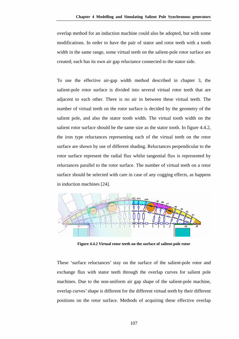
Chapter 4 Modelling and Simulating Salient Pole Synchronous generators
107
overlap method for an induction machine could also be adopted, but with some
modifications. In order to have the pair of stator and rotor teeth with a tooth
width in the same range, some virtual teeth on the salient-pole rotor surface are
created; each has its own air gap reluctance connected to the stator side.
To use the effective air-gap width method described in chapter 3, the
salient-pole rotor surface is divided into several virtual rotor teeth that are
adjacent to each other. There is no air in between these virtual teeth. The
number of virtual teeth on the rotor surface is decided by the geometry of the
salient pole, and also the stator tooth width. The virtual tooth width on the
salient rotor surface should be the same size as the stator tooth. In figure 4.4.2,
the iron type reluctances representing each of the virtual teeth on the rotor
surface are shown by use of different shading. Reluctances perpendicular to the
rotor surface represent the radial flux whilst tangential flux is represented by
reluctances parallel to the rotor surface. The number of virtual teeth on a rotor
surface should be selected with care in case of any cogging effects, as happens
in induction machines [24].
Figure 4.4.2 Virtual rotor teeth on the surface of salient-pole rotor
These ‘surface reluctances’ stay on the surface of the salient-pole rotor and
exchange flux with stator teeth through the overlap curves for salient pole
machines. Due to the non-uniform air gap shape of the salient-pole machine,
overlap curves’ shape is different for the different virtual teeth by their different
positions on the rotor surface. Methods of acquiring these effective overlap

Chapter 4 Modelling and Simulating Salient Pole Synchronous generators
108
curves and the reason to do so have been explained in chapter 3. As shown in
the left hand side of figure 4.4.2, virtual teeth #5 and #6 represent the flux
relationship between the salient-pole rotor tip (#5) or the area under the rotor
tip (#6) with the stator teeth to account for the fringing effect between the pole
tip and stator tooth, as shown in the circle in figure 4.4.1. Derived from FE
software, figure 4.4.3 shows these different overlap curves for different rotor
virtual teeth.
salient pole synchronous machine air gap overlap curves
-0.001
0
0.001
0.002
0.003
0.004
0.005
0.006
0.007
0.008
0.009
-0.3 -0.2 -0.1 0 0.1 0.2 0.3 0.4 0.5
offset (RAD)
air
gap
elem
ent e
ffec
tive
wid
th (m
)
10+11+12 7+8+9 5 6 2+3+4 1
air curve for #2,3,4 air curve for #1
air curve for #7,8,9
air curve for #10,11,12
air curve for #5
air curve for #6
Figure 4.4.3 Overlap curves for salient-pole synchronous machines
Offset (displacement) in figure 4.4.3 means the angular displacement between
the centres of each pair of teeth, as shown in figure 4.4.4.
Figure 4.4.4 Angular displacement of salient pole synchronous machine

Chapter 4 Modelling and Simulating Salient Pole Synchronous generators
109
It can be seen from the overlap curves above that curves #5 and #6 are not
symmetrical to the origin. The reason of this is that in the 0 offset point, when
the centre of tooth #5, #6 and one of the stator tooth are aligned, flux is shed
from coming into the rotor surface because the shape of the tip and the
definition of the centre on the virtual tooth. Thus, especially for tooth #6, the
maximum flux linkage happens in the position which has non-zero offset other
than the origin offset point where tooth #6 and the stator tooth centre are
aligned. The asymmetrical of curve #6 depends on how the centre of the virtual
tooth #6 is defined. The closer the centre of tooth #6 to the pole tip, the less
asymmetrical shape the air gap overlap curves have.
Another difficulty in air gap modelling is the non-uniform air gap length. The
length of the air gap reluctances of these virtual teeth are different due to their
different positions on the rotor surface. According to the usual pole geometry
of a salient pole generator, in order to get a more sinusoidal shape flux density
waveform on the air gap circumference, the salient pole shape is designed so
that the further the distance from the teeth to the pole centre, the longer the air
gap element length.
In the work discussed in this chapter, air gap lengths are calculated to be the
average value of the left end and right end of each air gap element connecting
each pair of virtual rotor teeth and stator teeth.
Virtual rotor teeth on the two sides of the salient-pole rotor are symmetrical
due to the symmetry of the pole. Their overlap shapes are also symmetrical
about the pole centre.
Flux distribution in electrical machines changes when the winding currents
change, and more leakage flux exists when the winding currents are large due
to the saturation characteristic of the iron material, such as in the transient of

Chapter 4 Modelling and Simulating Salient Pole Synchronous generators
110
the direct on line starting of induction machine and short circuit condition of
synchronous generator. In a synchronous generator, due to the large air gap in
between adjacent poles, in some running conditions, such as short circuit
testing, a certain leakage flux exists which could not be ignored. Some more air
gap reluctances must be additionally added to account for tip area leakage
fluxes between the pole tips, which are called inter-pole air gap reluctances in
DRM. These leakage and inter-pole reluctances are shown in Fig. 4.4.5.
Figure 4.4.5 Reluctance mesh shows the leakage air-gap reluctance
and inter-pole reluctances in salient-pole machine
M. G. Say suggests an empirical formula [27] of calculating leakage flux for a
low speed salient pole synchronous machine, as shown in equations 4.4.1 and
4.4.2.
• Flux between shoes (for each pole pair): 21 42 φφφ +=sl
⎥⎦
⎤⎢⎣
⎡⎟⎟⎠
⎞⎜⎜⎝
⎛++=
ss
s
sslsl c
bhchLF πµφ 5.01log9.22 100 (4.4.1)
• Flux between poles (for each pole pair): 43 42 φφφ +=pl
⎥⎥⎦
⎤
⎢⎢⎣
⎡⎟⎟⎠
⎞⎜⎜⎝
⎛++=
p
pp
p
pplpl c
bh
chL
Fπ
µφ5.0
1log5.1 100 (4.4.2)

Chapter 4 Modelling and Simulating Salient Pole Synchronous generators
111
where lF is the mmf of the winding, and parameter sL , pL , sh , ph , sc , pc b , pb are
shown in figure 4.4.5.
To fit the above equations representing leakage fluxes between salient poles
and pole shoes, corresponding inter pole reluctances representing these leakage
fluxes need to be added in to the Dynamic Reluctance Mesh modelling.
Assume reluctance 1ℜ represents the leakage flux 1φ , 2ℜ represents the leakage
flux 2φ , 3ℜ represents 3φ and 4ℜ represents 4φ . From equation 4.4.1, following
equations could be derived:
s
ssl c
hLF ⋅= 01 µφ (4.4.3)
4/5.01log9.2 1002 ⎟⎟⎠
⎞⎜⎜⎝
⎛+⋅=
ssl c
bhF πµφ (4.4.4)
Considering the relationship between flux and reluctance: ℜ= /lFφ ,
ss
s
hLc
01 µ=ℜ (4.4.5)
⎟⎟⎠
⎞⎜⎜⎝
⎛+
=ℜ
ss c
bh πµ 5.01log9.2
4
100
2 (4.4.6)
When considering the total leakage flux path between the pole shoes, based on
the leakage flux calculating method from M.G. Say, there are three parallel
leakage flux paths between each pair of pole shoes, as shown in figure 4.4.6,
which could be represented by:
221 //// ℜℜℜ=ℜsl (4.4.7)
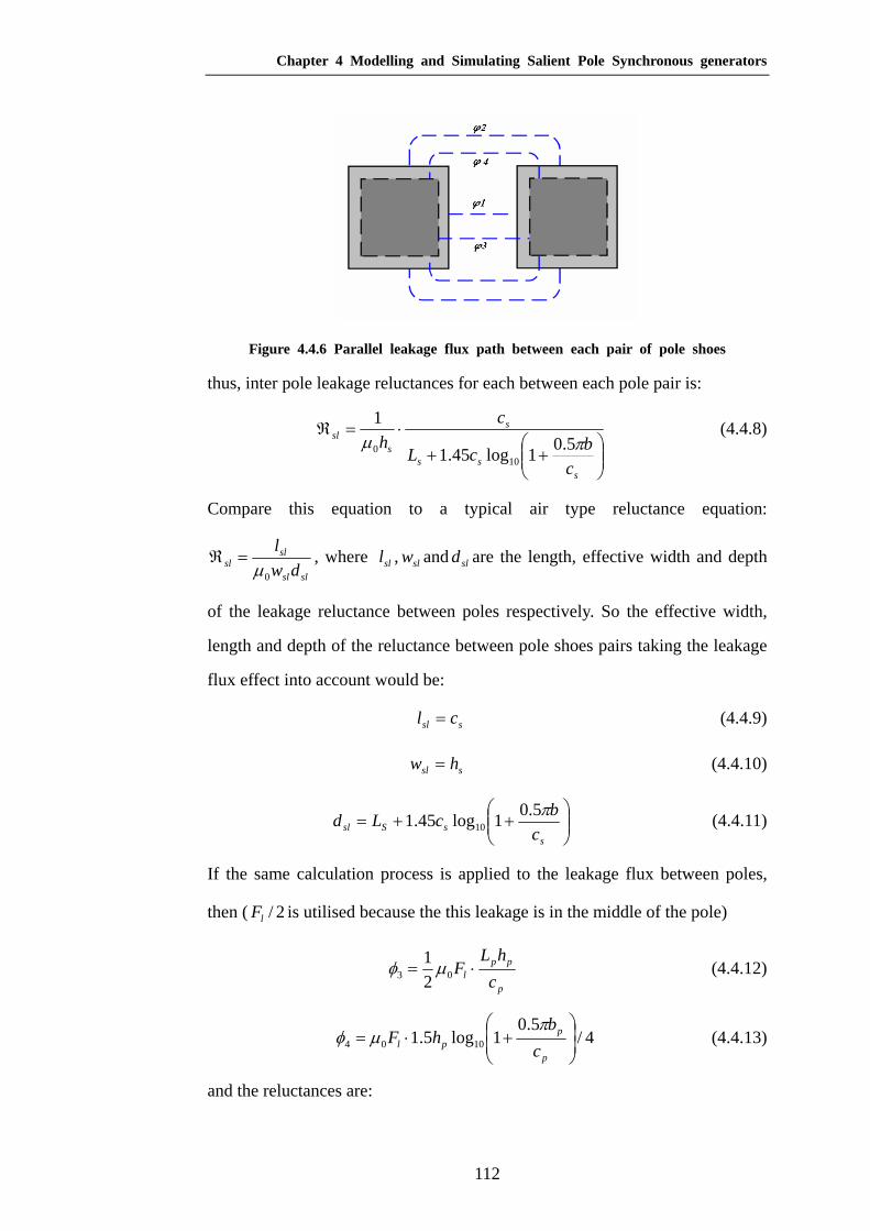
Chapter 4 Modelling and Simulating Salient Pole Synchronous generators
112
Figure 4.4.6 Parallel leakage flux path between each pair of pole shoes
thus, inter pole leakage reluctances for each between each pole pair is:
⎟⎟⎠
⎞⎜⎜⎝
⎛++
⋅=ℜ
sss
s
ssl
cbcL
ch πµ 5.01log45.1
1
100
(4.4.8)
Compare this equation to a typical air type reluctance equation:
slsl
slsl dw
l
0µ=ℜ , where sll , slw and sld are the length, effective width and depth
of the leakage reluctance between poles respectively. So the effective width,
length and depth of the reluctance between pole shoes pairs taking the leakage
flux effect into account would be:
ssl cl = (4.4.9)
ssl hw = (4.4.10)
⎟⎟⎠
⎞⎜⎜⎝
⎛++=
ssSsl c
bcLd π5.01log45.1 10 (4.4.11)
If the same calculation process is applied to the leakage flux between poles,
then ( 2/lF is utilised because the this leakage is in the middle of the pole)
p
ppl c
hLF ⋅= 03 2
1 µφ (4.4.12)
4/5.0
1log5.1 1004 ⎟⎟⎠
⎞⎜⎜⎝
⎛+⋅=
p
ppl c
bhF
πµφ (4.4.13)
and the reluctances are:

Chapter 4 Modelling and Simulating Salient Pole Synchronous generators
113
pp
p
hLc
03 µ=ℜ (4.4.14)
⎟⎟⎠
⎞⎜⎜⎝
⎛+
=ℜ
p
pp c
bh
πµ
5.01log5.1
2
100
4 , (4.4.15)
the leakage reluctance representing the leakage flux between poles are:
443 //// ℜℜℜ=ℜ pl (4.4.16)
⎟⎟⎠
⎞⎜⎜⎝
⎛++
⋅=ℜ
p
ppp
p
ppl
cb
cL
ch πµ 5.0
1log5.1
1
100
(4.4.17)
and the effective width, length and depth for leakage reluctance between the
poles are:
ppl cl = (4.4.18)
ppl hw = (4.4.19)
⎟⎟⎠
⎞⎜⎜⎝
⎛++=
p
ppppl c
bcLd
π5.01log5.1 10 (4.4.20)
With the inter pole leakage air gap reluctances modelled, the whole air gap
reluctance mesh of a salient pole rotor is shown in figure 4.4.7.
Figure.4.4.7 Whole air gap reluctance mesh for salient pole generator, including leakage
and inter-pole reluctances

Chapter 4 Modelling and Simulating Salient Pole Synchronous generators
114
4.4.2 Meshing of salient pole rotor
After finishing the modelling of the air gap part of the machine, this section
will continue to model the iron part of the generator. A salient pole
synchronous generator stator has a similar geometry to an induction machine
stator and the same reluctance mesh topology for induction machine could be
adopted. However, this is not the case in rotor reluctance mesh creation.
Because the rotor geometry for a salient-pole rotor generator and induction
machine are so different, the rotor mesh has to be quite different to in order to
account for the different flux distribution inside the rotor pole.
The advantage of Dynamic Reluctance Mesh is that the reluctance mesh could
be simplified by the given prior-known knowledge of flux distribution in the
machine. For a salient pole synchronous generator, the main flux distribution in
the salient pole is known from experience, thus the salient pole could be
discretised into the reluctance mesh based on empirical knowledge.
The main principle of dividing the iron part of a machine into reluctance mesh
is that the direction of the reluctances should be in approximately the same
direction as the flux direction, although some small displacements are allowed,
and there have to be reluctances where there is flux path. Reluctances should
lie in both radial and tangential directions in the iron to allow radial flux and
tangential flux to pass through, and reluctances in different direction can be
overlapped, because their fluxes have different directions.
Based on the discretisation principle given above, reluctance mesh for a
salient-pole rotor can be created as shown in figure 4.4.8.

Chapter 4 Modelling and Simulating Salient Pole Synchronous generators
115
Figure4.4.8 A typical complete salient pole rotor reluctance mesh
In the rotor surface region of a salient pole, reluctance mesh is modified due to
the presence of damper bars. A similar type of reluctance mesh for a cage rotor
in the induction machine is adopted here in the damper bar regions. One
reluctance represents the air gap element across the bar, and other elements
represent iron around the damper bar. In order to take account of the surface
flux in rotor, and also the flux flowing below the damper bar, two layers on the
top of the rotor surface are added. There are three elements between each pair
of damper bars because there might be some flux distortion between two
damper bars, as can be seen from the damper bar region in figure 4.4.8, thus an
additional central reluctance is added to account for the possible flux difference
between bars. Mmf sources are modelled in the same way were done with the
cage rotor induction machine.
In the meshing process, topology of the virtual teeth on the rotor surface
decides the topology inside the rotor, and these all depend on the approximate
flux distribution inside the pole. Thus, for the tangential direction, apart from
the first two layers which are situated at the damper area, another tangential

Chapter 4 Modelling and Simulating Salient Pole Synchronous generators
116
layer of reluctance mesh is needed which conduct the pole tip flux to the pole
centre, representing tangential flux across the pole, although it is normally
small. Also, a tangential path which accounts for the tangential flux path in the
middle of the yoke and connects with the inter pole leakage reluctances in the
leakage area, needs to be added to the reluctance mesh. In the shaft area, there
is also a tangential path to account for the circular flux around the shaft, as can
be seen in figure 4.4.8. The tangential reluctance mesh of the salient pole
generator is shown in figure 4.4.8.
As to the radial flux in the salient pole, the meshing process could be created
based on the discretisation of the virtual teeth on the salient rotor surface that
have already have been set up. Each virtual rotor tooth on the salient pole rotor
surface connects with one branch of reluctance mesh representing radial flux.
These radial reluctance branches are divided into central branch and pole tip
branch. Central branches will end up at the node around the shaft area, while
pole tip radial reluctance branch will end up at the pole tip area facing the shaft.
In central reluctance branches which represent the radial flux, two mmf sources
exists in each branch in the pole yoke area. This is due to the fact that one
tangential path separates the radial branch and thus there has to be two
reluctances in each of the radial branches. Since two mmf sources are situated
in each radial branch, the winding magnetomotive force has to be split evenly
between the two mmf sources. The radial flux reluctance mesh of a salient pole
generator could be shown in figure 4.4.8. Given the reluctance mesh shown in
figure 4.4.8 for the salient rotor pole, the flux in the pole tip area could flow to
anywhere inside the pole through the radial and tangential network, if mmf
potential difference exists.
4.4.3 Damper winding modelling
In previous sections, the dynamic reluctance mesh for the salient rotor

Chapter 4 Modelling and Simulating Salient Pole Synchronous generators
117
synchronous machine as well as the non-uniform air gap modelling has been
introduced. This section will concentrate on the modelling of the damper bars
in the salient pole. Some modelling approaches different to the methods that
have been adopted for induction machines will be used to model the damper
bar electrically and magnetically, because of the irregular spacing of these
damper bars on the salient rotor surface. Details of damper bar modelling for a
salient pole synchronous rotor will be given in this section.
Damper bars are acknowledged as one of the most important method to reduce
the instability during synchronisation or rapid change in load for salient pole
generators. Thus damper bar modelling is a very important aspect in simulating
a practical salient-pole synchronous machine.
Damper bars here are different from that of induction machines in that they are
not equally spaced and the reluctances between each damper bar is not just one.
The DRM principle of modelling mmfs is that: a magnetic loop requires that no
‘fake’ internal loop should exist, so that no ‘fake’ flux would exist in the
proposed reluctance meshing solution. Thus, if one mmf source were added for
each damper bar, as shown by the circles in the radial direction flux branch, in
figure 4.4.9, there would be ‘fake’ internal flux circulating around the bars, as
shown by the arrow in figure 4.4.9. To eliminate these ‘fake’ internal fluxes,
other reluctance mesh topology for damper bars has to be proposed.
Figure 4.4.9 Reluctance mesh topology for modelling of damper bars
which has ‘fake’ internal flux loop
To solve this, some virtual damper bars are added, as the way done to virtual

Chapter 4 Modelling and Simulating Salient Pole Synchronous generators
118
rotor teeth for the salient pole. Thus, there is one damper bar associated with
each virtual tooth on the salient pole rotor surface, some of the damper bars are
real and some are virtual ones, as shown in figure 4.4.10.
Figure 4.4.10 Virtual Damper Bars and mmfs
By modelling the damper bars as shown in figure 4.4.10, there is no possible
fake internal flux circulation existing in the reluctance mesh. In the DRM
simulations, the real damper bars and virtual damper bars are discriminated by
their resistance: real ones have normal bar resistance, while virtual ones have a
very big resistance to stop the current flowing through, such that there is no
physical influence by the adding of these virtual damper bars.
Each virtual rotor tooth has a damper bar associated with it now, either a real
damper bar or a virtual one. Thus, a salient-pole rotor dynamic reluctance
model is unified with an induction machine rotor dynamic reluctance model,
and the same electrical loop model could be applied from the induction
machine.
As to the right-most flux branch in the salient pole rotor mesh, the virtual
damper bar is positioned between two poles. This is a realistic assumption
because damper bars on one pole are physically connected with the damper
bars on another pole by the short circuit straps [27]. These are made with
copper, as show in figure 4.4.11. The DRM model for virtual bars between the

Chapter 4 Modelling and Simulating Salient Pole Synchronous generators
119
two poles can be shown in figure 4.4.12.
Figure 4.4.11 Real damper bar construction between two poles
Figure 4.4.12 Virtual damper bar modelling between two salient-poles
With the models of damper bars that have been set up, a DRM model creation
of the whole salient-pole synchronous generator could be completed. A
complete salient-rotor reluctance mesh is shown in figure 4.4.13.

Chapter 4 Modelling and Simulating Salient Pole Synchronous generators
120
Figure 4.4.13 Proposed complete salient pole rotor reluctance mesh
After completing the creation of the reluctance mesh and the modelling of the
damper bars and air gap, a complete DRM model for the salient pole rotor and
air gap were set up. The stator reluctance mesh could be similar to that of an
induction machine, due to the similar geometry and flux distribution inside the
stator. In the following section, the state equations and state variables for the
single salient pole synchronous generator will be given, to simulate the
machine behaviour.
4.4.4 Equations and state variables for salient pole machine
The operating condition of a usual synchronous machine is that the shaft, to
which the salient pole rotor is connected, is driven by a prime mover rotating at
synchronous speed. Excitation voltage is applied to the rotor terminals, and a.c.
currents are generated on the stator side by the relative rotation of the flux
fields and the stationary stator coils.
To solve for the system state, and thus calculate the machine performance,
system equations have to be given out. This section will give the state variables

Chapter 4 Modelling and Simulating Salient Pole Synchronous generators
121
describing the system state and the system state equations.
The equations describing the node mmf potentials are the same for different
types of machine in a DRM modelling method, as long as they have magnetic
circuits. Similar to that of induction machines, equation 4.4.21 is satisfied for
each node connecting the reluctances for a salient pole synchronous generator.
( ) 0, 12
1
0=∑
−
=jjj
n
jmmfmmfφ (4.4.21)
The rotor electrical circuit equation is:
0=++−dt
dRiv f
fff
φ (4.4.22)
where fv , fi and fR are the terminal voltage, field current and resistance of the
rotor, andφ is the flux flowing through the field winding.
Damper bar circuit equations almost have the same format as that for induction
machines cage bars, after the modification of the modelling by virtual damper
bars. Thus, electrical equations for adjacent damper bars are:
011 =−⋅+⋅− −− dtdRiRi iiiiφ
(4.4.23)
iii mmfmmfi −= +1 (4.4.24)
Parameters here have the same specification as that in chapter 2.
Stator three phase electrical equations are as same as that of induction
machines:
01
=⋅+⋅+− ∑=
S
i
i
i
aaaA dt
dddeiRv φφ
(4.4.25)
01
=⋅+⋅+− ∑=
S
i
i
i
bbbB dt
dddeiRv φφ
(4.4.26)
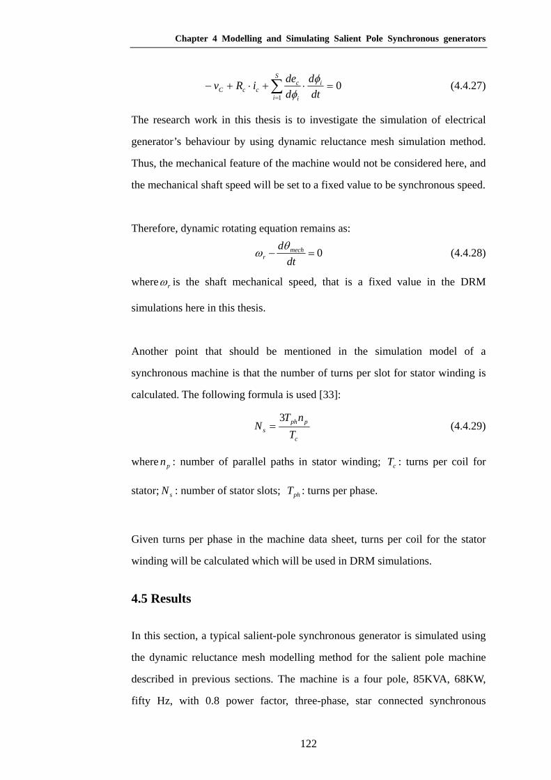
Chapter 4 Modelling and Simulating Salient Pole Synchronous generators
122
01
=⋅+⋅+− ∑=
S
i
i
i
cccC dt
dddeiRv φφ
(4.4.27)
The research work in this thesis is to investigate the simulation of electrical
generator’s behaviour by using dynamic reluctance mesh simulation method.
Thus, the mechanical feature of the machine would not be considered here, and
the mechanical shaft speed will be set to a fixed value to be synchronous speed.
Therefore, dynamic rotating equation remains as:
0=−dt
d mechr
θω (4.4.28)
where rω is the shaft mechanical speed, that is a fixed value in the DRM
simulations here in this thesis.
Another point that should be mentioned in the simulation model of a
synchronous machine is that the number of turns per slot for stator winding is
calculated. The following formula is used [33]:
c
pphs T
nTN
3= (4.4.29)
where pn : number of parallel paths in stator winding; cT : turns per coil for
stator; sN : number of stator slots; phT : turns per phase.
Given turns per phase in the machine data sheet, turns per coil for the stator
winding will be calculated which will be used in DRM simulations.
4.5 Results
In this section, a typical salient-pole synchronous generator is simulated using
the dynamic reluctance mesh modelling method for the salient pole machine
described in previous sections. The machine is a four pole, 85KVA, 68KW,
fifty Hz, with 0.8 power factor, three-phase, star connected synchronous

Chapter 4 Modelling and Simulating Salient Pole Synchronous generators
123
generator. The schematic drawing of the machine electrical connection is
shown in figure 4.5.1.
Figure 4.5.1 Schematic drawing of electrical connection for the generator to be simulated
In the testing that is done in this section, the rotor is excited by a d.c. voltage.
In practise, a rotor terminal is usually fed by an exciter, which is actually
another a.c. generator, through a rotating rectifier. However, it is excited
directly through d.c. voltage in the tests in this chapter, for the reason that a
single generator test is wanted, rather than a complicated system testing.
Testing for the complete system will be performed in the next chapter.
An open circuit test and a short circuit test with the DRM model will be
presented in this section, and also the results compared to the experimental
results. System performance with and without damper bars in sudden short
circuit condition is also simulated and investigated.
4.5.1 Open circuit & short circuit test
Testing conditions for open circuit test is: large resistive load is connected to
the stator three-phase to simulate open circuit conditions. The big resistance
virtually limits the phase current such that stator open circuit condition is
simulated numerically. Different rotor excitation voltages are applied to rotor
terminals, and stator terminal line-to-line voltages are recorded as the output
voltage. The rotor speed is fixed to the synchronous speed numerically as

Chapter 4 Modelling and Simulating Salient Pole Synchronous generators
124
mentioned in the previous section.
Experimental data of the open circuit and short circuit test is shown in figure
4.5.2.
Open Circuit & Short Circuit Test
52.9
100.6
151.4
202.8
259.9
300.2
350.2
382.0
403.6416.0
440.4
480.0
500.8
520.0
541.0
10.000
31.000
61.700
92.800
122.700
156.500
184.200
0.0
50.0
100.0
150.0
200.0
250.0
300.0
350.0
400.0
450.0
500.0
550.0
600.0
0.000 10.000 20.000 30.000 40.000 50.000 60.000
Generator Rotor Current (Amps)
Gen
erat
or st
ator
vol
tage
(Vol
ts)
0.000
25.000
50.000
75.000
100.000
125.000
150.000
175.000
200.000
225.000
250.000
275.000
300.000
Gen
erto
r st
ator
Cur
rent
(Am
ps)
Open Circuit Test Short Circuit Test
Short Circuit Test
Open Circuit Test
Figure 4.5.2 Experimental result of open circuit test and short circuit test

Chapter 4 Modelling and Simulating Salient Pole Synchronous generators
125
The DRM result for the open circuit test is shown in figure 4.5.3. As can be
seen, the simulation result is quite close to the experimental results, especially
in the rated generating voltage area, which is 400 volts. Maximum error in the
result comparison is –8.7%, and the average error in percentage is 2.5%, which
is excellent for engineering simulations. The relatively big error in the result
with the increasing of field current is due to the material saturation. The
material used in a DRM simulation is slightly different from that used in the
experimental result. Thus, the small difference in material saturation
characteristic can cause the result difference in figure 4.5.3. Iron material that
has been used in DRM simulation is Losil 800 for both the stator and the rotor,
while the material used in the real machine is Losil 800 for the rotor and
DK70-65 for the stator.

Chapter 4 Modelling and Simulating Salient Pole Synchronous generators
126
Open circuit test results comparison between DRM and experimental data
52.9
100.6
151.4
202.8
259.9
300.2
350.2
382.0
403.6416.0
440.4
480.0
500.8
520.0
541.0
0.0
50.0
100.0
150.0
200.0
250.0
300.0
350.0
400.0
450.0
500.0
550.0
600.0
0.000 10.000 20.000 30.000 40.000 50.000 60.000
Generator rotor current (Amps)
Gen
erat
or st
ator
vol
tage
(Vol
ts)
-10
-8
-6
-4
-2
0
2
4
6
Err
or%
experimental data DRM result Error
experimental result
DRM result
Error
Figure 4.5.3 Open circuit result comparison for DRM and experiment data
In DRM simulations, rotor resistance rise with regards to temperature is also
considered by using rotor resistance calculated from the experimental data
sheet.
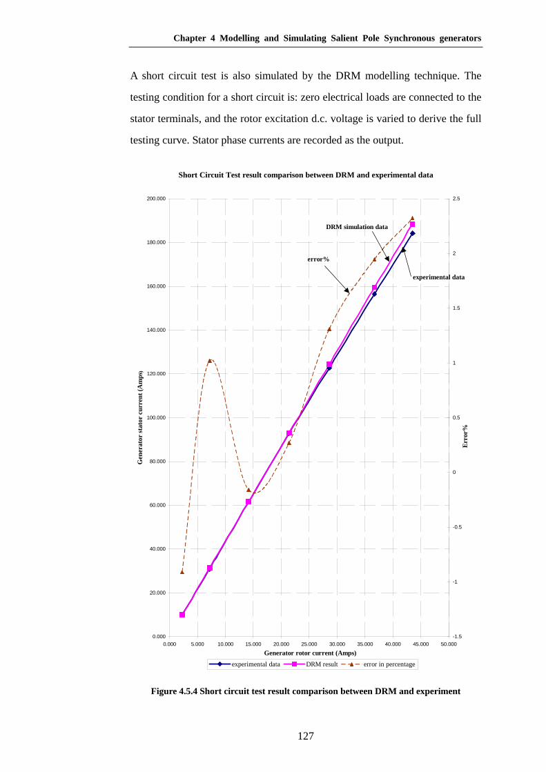
Chapter 4 Modelling and Simulating Salient Pole Synchronous generators
127
A short circuit test is also simulated by the DRM modelling technique. The
testing condition for a short circuit is: zero electrical loads are connected to the
stator terminals, and the rotor excitation d.c. voltage is varied to derive the full
testing curve. Stator phase currents are recorded as the output.
Short Circuit Test result comparison between DRM and experimental data
0.000
20.000
40.000
60.000
80.000
100.000
120.000
140.000
160.000
180.000
200.000
0.000 5.000 10.000 15.000 20.000 25.000 30.000 35.000 40.000 45.000 50.000
Generator rotor current (Amps)
Gen
erat
or st
ator
cur
rent
(Am
ps)
-1.5
-1
-0.5
0
0.5
1
1.5
2
2.5
Err
or%
experimental data DRM result error in percentage
experimental data
DRM simulation data
error%
Figure 4.5.4 Short circuit test result comparison between DRM and experiment

Chapter 4 Modelling and Simulating Salient Pole Synchronous generators
128
Figure 4.5.4 shows the short circuit test result comparison between the DRM
simulation result and the experimental result. They are quite close, and error is
within 2.5%, with an average error of 1.135%, which is excellent for
engineering simulations. Again, the relatively big error in the saturation region
is due to the different material used in the DRM simulations compared to that
used in the experiment.
4.5.2 Sudden short circuit test
Sudden short circuit conditions are important in generator performance
evaluations, and could cause great damage if not properly treated. In this
section, sudden short circuit condition of synchronous generators will be
simulated, and the effect of damper bars during the sudden short circuit
condition will be investigated, by using a DRM simulation tool.
Sudden Short Circuit Test; Stator line-to-line Voltage
-800
-600
-400
-200
0
200
400
600
800
3.2 3.3 3.4 3.5 3.6 3.7 3.8 3.9 4
Time (s)
Stat
or L
ine-
Lin
e V
Olta
ge (V
olts
)
Figure 4.5.5 Sudden short circuit test, stator line-to-line voltage
Figure 4.5.4 shows the generator stator terminal voltage waveforms during
sudden short circuit operating conditions. The short circuit happens at 3.5
seconds. It can be seen that the stator terminal line-to-line voltage value
becomes very small as expected.

Chapter 4 Modelling and Simulating Salient Pole Synchronous generators
129
Figures 4.5.6 to 4.5.9 show the changing of stator phase current and field
current during sudden short circuit transients. Due the theorem of constant
linkage [27], flux linkage in an inductive magnetic circuit tends to remain the
flux to be a constant level when there is a sudden flux change in the circuit.
Thus, rotor current response to the sudden change of flux generated by sudden
change of stator short circuit currents, and very large rotor current generated.
Actually, these rotor current variations take place partly in the rotor winding,
partly in other closed paths available for current flow, such as damper
windings.
Sudden Short Circuit test: stator phase A Current
-1500
-1000
-500
0
500
1000
1500
2000
2500
3.2 3.3 3.4 3.5 3.6 3.7 3.8 3.9 4
Time(s)
Stat
or c
urre
nt(A
)
no damper bars with damper bars
with damper bars
no damper bars
Figure 4.5.6 Sudden short circuit test stator phase current

Chapter 4 Modelling and Simulating Salient Pole Synchronous generators
130
sudden short circuit test, stator phase B current
-1500
-1000
-500
0
500
1000
1500
2000
2500
3.2 3.3 3.4 3.5 3.6 3.7 3.8 3.9 4
Time(s)
stat
or p
hase
B c
urre
nt (A
mps
)
no damper bars with damper bars
with damper bars
no damper bars
Figure 4.5.7 Sudden short circuit test, stator phase B current
Sudden Short Circuit Test: stator phase C current
-3000
-2500
-2000
-1500
-1000
-500
0
500
1000
3.2 3.3 3.4 3.5 3.6 3.7 3.8 3.9 4
Time (S)
Stat
or C
urre
nt (A
)
no damper bars with damper bars
with damper bars
no damper bars
Figure 4.5.8 Sudden short circuit test, stator phase C current
At the moment of short circuit of a three-phase machine, the flux linking the
stator from the rotor is caught and ‘frozen’ to the stator, giving a stationary
replica of the main-pole flux. For this purpose each phase will, in general, carry
a d.c. component, which will cause d.c. offset or asymmetry in the waveform
of the stator current with respect to time, and will disappear with time. The
quantity of d.c. offset depends the relative position of the stator and rotor in the

Chapter 4 Modelling and Simulating Salient Pole Synchronous generators
131
instance of short circuit. As can be seen from figures 4.5.6-4.5.8, d.c offset is
different for the stator three phase current.
The initial short circuit currents are limited by the transient reactance dx′ and
sub-transient reactance dx ′′ , which characterises the effective leakage inductance.
The steady state short circuit current, however, is limited by dx , where dx is the
synchronous reactance of the generator.
sudden short circuit, field current
0
50
100
150
200
250
300
350
400
3.2 3.3 3.4 3.5 3.6 3.7 3.8 3.9 4
Time (s)
Fiel
d cu
rren
t (A
mps
)
no damper bars with damper bars
with damper bars
no damper bars
Figure 4.5.9 Sudden short circuit test, generator field current

Chapter 4 Modelling and Simulating Salient Pole Synchronous generators
132
Sudden Short Circuit Test: Damper Bar Current
-2000
0
2000
4000
6000
8000
10000
12000
14000
3.2 3.3 3.4 3.5 3.6 3.7 3.8 3.9 4
Time(s)
Dam
per
Bar
Cur
rent
(Am
ps)
Figure 4.5.10 Sudden short circuit test, damper bar current
Damper winding plays an important part in synchronous machine transient. It
reduces the oscillations in currents and helps maintain mechanical stability. As
shown in figures 4.5.6-4.5.10, compared with the machine that has damper
windings, stator phase currents of the generator that has no damper winding are
lower and field current is more in a sudden short circuit case. This is because
the damper bar is a part of the rotor windings, and it accounts for part of flux
change in the whole rotor windings, apart from the field winding. A simple
comparison for the current between the machine with damper bars and without
damper bars is shown in table 5.1.
Field current Stator phase current
No damper bar generator more less
Damper bar generator less more
Table 5.1 Comparison of currents in generators with and without damper bars
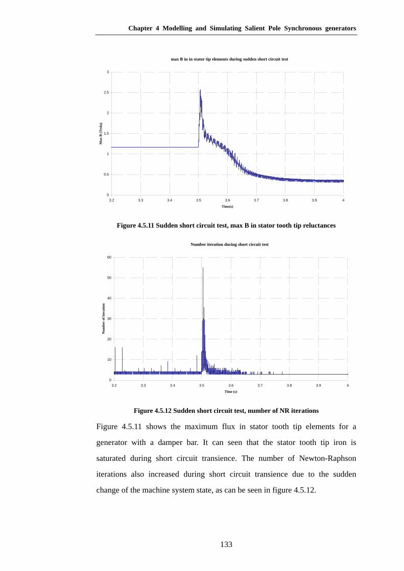
Chapter 4 Modelling and Simulating Salient Pole Synchronous generators
133
max B in in stator tip elements during sudden short circuit test
0
0.5
1
1.5
2
2.5
3
3.2 3.3 3.4 3.5 3.6 3.7 3.8 3.9 4
Tims(s)
Max
B (T
esla
)
Figure 4.5.11 Sudden short circuit test, max B in stator tooth tip reluctances
Number iteration during short circuit test
0
10
20
30
40
50
60
3.2 3.3 3.4 3.5 3.6 3.7 3.8 3.9 4
Time (s)
Num
ber
of it
erat
ion
Figure 4.5.12 Sudden short circuit test, number of NR iterations
Figure 4.5.11 shows the maximum flux in stator tooth tip elements for a
generator with a damper bar. It can seen that the stator tooth tip iron is
saturated during short circuit transience. The number of Newton-Raphson
iterations also increased during short circuit transience due to the sudden
change of the machine system state, as can be seen in figure 4.5.12.

Chapter 4 Modelling and Simulating Salient Pole Synchronous generators
134
4.5.3 Damper bar investigation
With the help of DRM software, the damper bar effects in synchronous
machines could be investigated. Figure 4.5.13 shows the damper bar currents in
open circuit running conditions.
damper bar current comparison
-3
-2
-1
0
1
2
3
3 3.005 3.01 3.015 3.02 3.025 3.03 3.035 3.04
time(s)
dam
per b
ar c
urre
nt (A
mps
)
bar current 4 bar current 7
bar current 7
bar current 4
Figure 4.5.13 Adjacent Damper bar currents
Figure 4.5.13 shows the adjacent damper bar currents. As can be seen from the
figure, there are phase offsets between the currents of adjacent bars. They are
caused by the different damper bar positions on the salient rotor pole surface.
Thus, current in one damper bar leads the current in the next bar following the
rotating direction. The phase offset between the currents depends on both the
speed of the rotor and the distance between the bars.
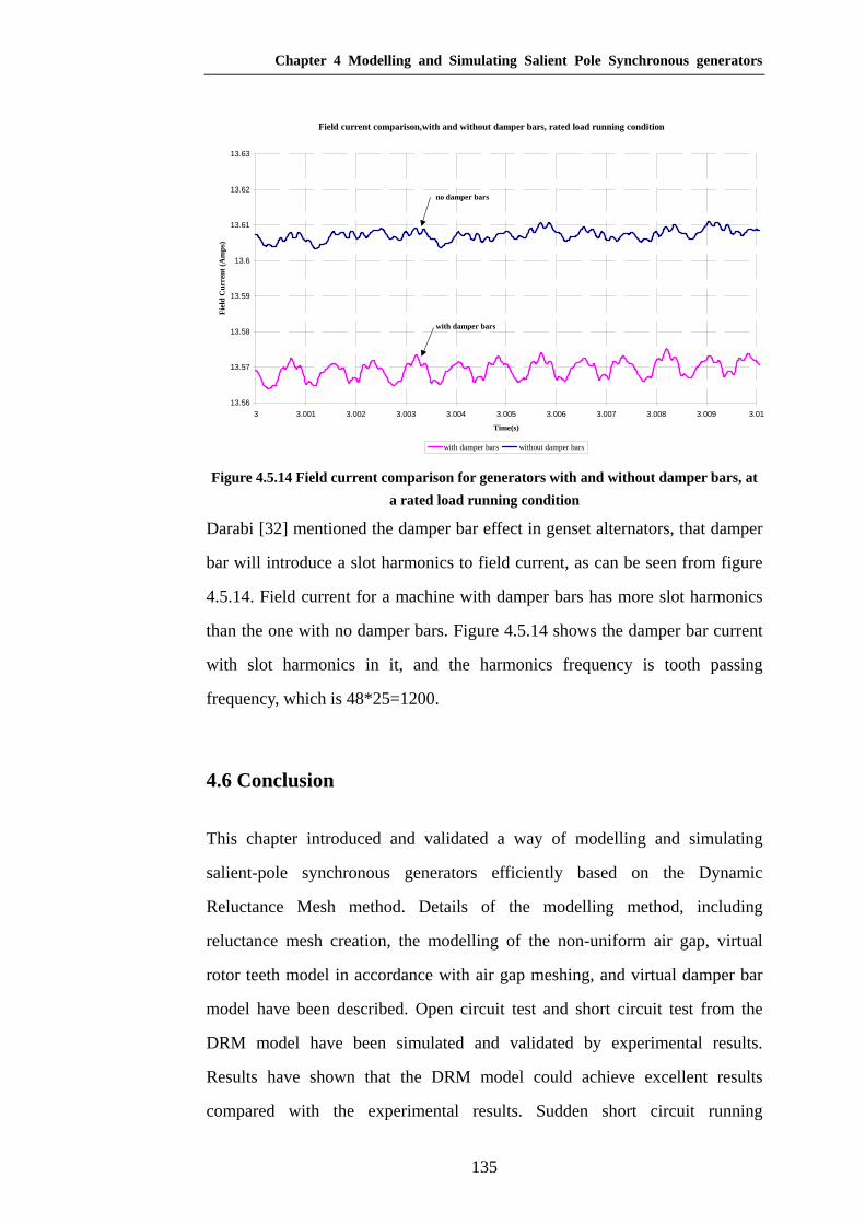
Chapter 4 Modelling and Simulating Salient Pole Synchronous generators
135
Field current comparison,with and without damper bars, rated load running condition
13.56
13.57
13.58
13.59
13.6
13.61
13.62
13.63
3 3.001 3.002 3.003 3.004 3.005 3.006 3.007 3.008 3.009 3.01
Time(s)
Fiel
d C
urre
nt (A
mps
)
with damper bars without damper bars
no damper bars
with damper bars
Figure 4.5.14 Field current comparison for generators with and without damper bars, at
a rated load running condition
Darabi [32] mentioned the damper bar effect in genset alternators, that damper
bar will introduce a slot harmonics to field current, as can be seen from figure
4.5.14. Field current for a machine with damper bars has more slot harmonics
than the one with no damper bars. Figure 4.5.14 shows the damper bar current
with slot harmonics in it, and the harmonics frequency is tooth passing
frequency, which is 48*25=1200.
4.6 Conclusion
This chapter introduced and validated a way of modelling and simulating
salient-pole synchronous generators efficiently based on the Dynamic
Reluctance Mesh method. Details of the modelling method, including
reluctance mesh creation, the modelling of the non-uniform air gap, virtual
rotor teeth model in accordance with air gap meshing, and virtual damper bar
model have been described. Open circuit test and short circuit test from the
DRM model have been simulated and validated by experimental results.
Results have shown that the DRM model could achieve excellent results
compared with the experimental results. Sudden short circuit running

Chapter 4 Modelling and Simulating Salient Pole Synchronous generators
136
conditions and the effect of damper bars have also been simulated and
investigated.
Compared with the Finite Element Method, results that come out of the DRM
model are quite satisfied, both with accuracy and speed. Thus this Dynamic
Reluctance Mesh model could provide a faster and more effective way of
simulating salient-pole synchronous generators in engineering solutions, which
can be used in further analysis such as generator system simulations and
investigations, where currently commercial FEM software was not able to cope.
This will be mentioned further in later chapters.

Chapter 5 Simulation and Investigation of Brushless Generating System ——————————————————————————————————————
137
CHAPTER 5 SIMULATION AND INVESTIGATION OF
BRUSHLESS GENERATING SYSTEM
5.1 Introduction
In this chapter, the DRM models for brushless generating systems, including
the models of the exciter, the rotating rectifiers, and the automatic voltage
regulator (AVR) will be discussed. The DRM model for the main generator has
been described and validated in chapter 4 and will not be given here.
This work is a significant advance on conventional methods of simulating a
generator system. Normally, system models are analysed using programs like
MATLABTM Simulink where conventional sinusoidal dq machine models are
employed. Such machine models are very limited and neglect many saturation,
harmonic and slotting effects inherent in a practical machine. Modelling using
the detailed field models of machines is also normally confined to a single
machine at a time such as a generator. That is system models are not examined.
The work presented in this chapter includes detailed field models of both the
generator and exciter as well as models covering the rotating rectifier and AVR
all. That is the complete system is simulated at one time with the entire
practical machine features included. This approach ensures that design of the
system can be highly refined and critical operating conditions associated with
voltage recovery following a fault can be optimised.
The work presented includes an initial examination of generator and exciter
systems to show that the system chosen is the most appropriate for general
study. Generator systems normally comprise the excitation systems, which
supply d.c. current to synchronous generators field winding, although some

Chapter 5 Simulation and Investigation of Brushless Generating System ——————————————————————————————————————
138
small generators are sometimes built with permanent-magnet field excitations.
Since the rotor is rotating, a special arrangement is required to get the d.c.
power to its field windings. There are several common approaches to supplying
this d.c. power [34] [35]:
1. Supply the d.c. power from an external d.c. generator to the rotor by means
of slip rings and brushes, as shown in figure 5.1.1. D.c. current is generated
by a d.c. generator whose rotor is mounted on the same shaft with the main
generator rotor, and the generated d.c. voltage is connected to the main rotor
field winding through the slip rings and brushes. This excitation method
creates a few problems, when it is used to supply d.c. power to the field
windings of a synchronous machine. It increases the amount of maintenance
required on the machine and brush voltage drop can be the cause of
significant power losses on machines with larger field currents. Despite
these problems, slip rings and brushes were used on smaller synchronous
machines, because no other method of supplying the d.c. field current was
cost-effective.
Figure 5.1.1 Conventional excitation of generator systems
2. There is also another choice, which is static excitation for the synchronous
generator systems. There are no rotating parts in this excitation system, and
the excitation power is supplied from the generated voltage itself, as shown
in figure 5.1.2. Generated voltage from the main generator comes to a static
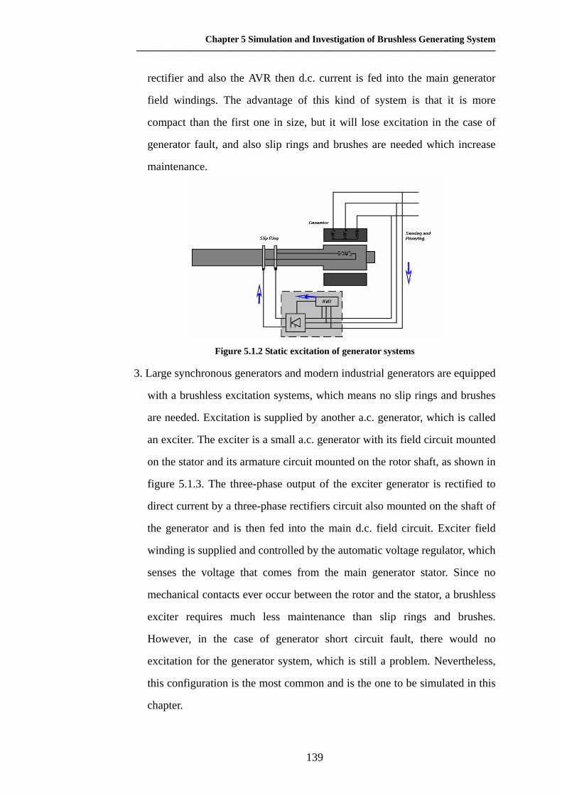
Chapter 5 Simulation and Investigation of Brushless Generating System ——————————————————————————————————————
139
rectifier and also the AVR then d.c. current is fed into the main generator
field windings. The advantage of this kind of system is that it is more
compact than the first one in size, but it will lose excitation in the case of
generator fault, and also slip rings and brushes are needed which increase
maintenance.
Figure 5.1.2 Static excitation of generator systems
3. Large synchronous generators and modern industrial generators are equipped
with a brushless excitation systems, which means no slip rings and brushes
are needed. Excitation is supplied by another a.c. generator, which is called
an exciter. The exciter is a small a.c. generator with its field circuit mounted
on the stator and its armature circuit mounted on the rotor shaft, as shown in
figure 5.1.3. The three-phase output of the exciter generator is rectified to
direct current by a three-phase rectifiers circuit also mounted on the shaft of
the generator and is then fed into the main d.c. field circuit. Exciter field
winding is supplied and controlled by the automatic voltage regulator, which
senses the voltage that comes from the main generator stator. Since no
mechanical contacts ever occur between the rotor and the stator, a brushless
exciter requires much less maintenance than slip rings and brushes.
However, in the case of generator short circuit fault, there would no
excitation for the generator system, which is still a problem. Nevertheless,
this configuration is the most common and is the one to be simulated in this
chapter.

Chapter 5 Simulation and Investigation of Brushless Generating System ——————————————————————————————————————
140
Figure 5.1.3 Brushless excitation of generator systems
4. To make the excitation of a generator completely independent of any
external power sources, a small pilot exciter is often included in the system.
A pilot exciter is a small a.c. generator with permanent magnets mounted on
the rotor shaft and a three-phase winding on the stator. It produces the
power for the field circuit of the exciter, as shown in figure 5.1.4, which in
turn controls the field circuit of the main machine.
Figure 5.1.4 Brushless excitation with pilot exciter of generator system
It is not common for people to simulate the generating system including main
generator, exciter and AVR altogether, because this involves two machines and
also the power electronic components as the state equations need to be solved
simultaneously. For a simple mathematical machine model, the whole system
state equations may be solved. However, for the latest Finite Element
technology, commercial software could not simulate two machines at the same
time, although it might be possible in the near future. Darabi [36] simulated the
Chapter 5 Simulation and Investigation of Brushless Generating System ——————————————————————————————————————
141
brushless generator system with a small salient-pole synchronous machine and
an exciter including AVR using FEM. However, the exciter model was not an
FE model but a parametric model based on self and mutual inductances.
Due to the great flexibility and efficiency of Dynamic Reluctance Modelling
technology, the complete brushless generating system including the exciter, the
rotating rectifiers and the main generator, and voltage regulator, as the system
shown in figure 5.1.3, can be simulate simultaneously. However, the AVR that
is modelled here in this chapter is quite a simple model. It would not be a
problem to utilize a more advanced AVR model and control algorithms into the
generating system, so that the more realistic voltage regulation could be
investigated. Even for the brushless generating system including the pilot
exciter, the DRM could accommodate this kind of simulation without a great
effort. It would all just require more work and the objective here is to show
how the full field models of two or more machines can be incorporated with
the control algorithm quite easily using the DRM approach.
In this chapter, the complete brushless generator system, including exciter,
rectifiers and main generator and a simple automatic voltage regulator will be
modelled. The generator model using the DRM has been described in chapter 4,
and results have shown that the DRM model gives good accuracy from an
engineering point of view. Exciter modelling will be described firstly in this
chapter, and the rectifier model described next together with the system
equations and state variables. Simulation results are given together with
experimental results to justify this part of the model. Then the design and
modelling of the AVR controller is described. Finally, the DRM simulations
result of the complete brushless generating system are then described and
discussed.

Chapter 5 Simulation and Investigation of Brushless Generating System ——————————————————————————————————————
142
5.2 Exciter Modelling Scheme
The exciter is effectively a reversed synchronous machine with field winding
staying on the stator and armature winding staying on the rotor side. The
exciter geometry that is to be modelled in this chapter is shown in figure 5.2.1.
Details of the exciter can be found in appendix 7.
Figure 5.2.1 Exciter geometry, with field winding staying on the stator and
armature winding on the rotor
5.2.1 Meshing the exciter
Based on the geometry of the exciter stator and rotor shown in figure 5.2.1, the
same kind of meshing schemes for to the induction machine given in chapter 2
are applied to the exciter discretisation process. The only difference in the
discretisation from that of the induction machine is that there is less number of
stator teeth in the stator of exciter. Considering that there will be leakage flux
flowing through the stator slots and rotor slots, for the reason described in
chapter 3.5, and that saturation of the teeth will probably be high, one
additional reluctance representing the leakage flux crossing the slots between
the two teeth is included. The cross-section of the typical exciter reluctance
mesh is shown in figure 5.2.2.

Chapter 5 Simulation and Investigation of Brushless Generating System ——————————————————————————————————————
143
Figure 5.2.2 Sections of exciter reluctance mesh model
Hollow rectangles in figure 5.2.2 represent the iron reluctances, the circle is the
mmf source due to winding currents, and filled rectangles are the air type
reluctances, including leakage reluctances between slots and dynamic air gap
reluctances connecting stator and rotor teeth. The method of calculating the
reluctances is the same as described in chapter2.
5.2.2 Air gap reluctance curve of the exciter
Air gap reluctance curve method, which is named for method 3 in chapter 3,
can be applied to different kinds of machines, and the number of reluctance
curves depends on the detailed air gap geometry. There is only one air gap
reluctance curve for the induction machine due to its uniformed air gap length
and the similar width for the stator and rotor teeth. Several air gap reluctance
curves are essential for salient pole synchronous machines due to their
non-uniform air gap length design and the very big inter-pole area, which
makes inter pole leakage flux significant.

Chapter 5 Simulation and Investigation of Brushless Generating System ——————————————————————————————————————
144
By applying the method described in chapters 3 and 4, the air gap reluctance
curves for the exciter machine can be derived. In deriving the air gap
reluctance curve, the excitation coil is put on the rotor side, as has been done
with both induction machine and synchronous machines. Fluxes entering into
each virtual stator tooth are then evaluated. Thus the effective flux linkage
between a virtual stator tooth and a rotor tooth can be calculated for different
offset positions in the form of the effective width of uniform air gap
reluctances. Figure 5.2.3 shows the air gap reluctance curve for this type of
exciter machine.
Air gap curves for exciter
-0.002
0
0.002
0.004
0.006
0.008
0.01
0.012
-0.3 -0.2 -0.1 0 0.1 0.2 0.3
Offset (RAD)
Eff
ectiv
e w
idth
(m)
CENTRAL SIDE
Figure 5.2.3 Exciter air gap reluctance curves
There are two curves in the figure, which are for the central and side virtual
teeth for the stator respectively. 3 virtual teeth exist on the stator teeth of the
exciter, for the reason that the relatively wider stator teeth width compared to
that of the rotor. Comparison of the simulation results from different number of
virtual teeth will be made in chapter 7 later.
5.2.3 Exciter machine system equations
In creating the system equations, the equations for the node mmfs are the same
for all types of machines, independent of machine geometry.

Chapter 5 Simulation and Investigation of Brushless Generating System ——————————————————————————————————————
145
( ) 0,1
012 =∑
−
=
n
jjjj mmfmmfφ (5.2.1)
Equation for the electrical circuit of the field winding, which is staying on the
stator side for an exciter, is:
0=++−dt
dRiV f
fff
φ (5.2.2)
Equations for the electrical circuit of the armature windings, which are
staying on rotor for an exciter, are:
01
=⋅+⋅+− ∑=
S
i
i
i
aaaA dt
dddeiRv φφ
(5.2.3)
01
=⋅+⋅+− ∑=
S
i
i
i
bbbB dt
dddeiRv φφ
(5.2.4)
01
=⋅+⋅+− ∑=
S
i
i
i
cccC dt
dddeiRv φφ
(5.2.5)
The dynamic equation for rotating angle is:
0=−dt
d mechr
θω (5.2.6)
5.2.4 Simulation results
With the dynamic reluctance mesh model set up for the exciter, simulations
have been done to verify the functioning of this model. An open circuit
condition for the rotor starting with zero field current and an applied field
voltage has been examined and the results are shown in following figures.

Chapter 5 Simulation and Investigation of Brushless Generating System ——————————————————————————————————————
146
Exciter stator current-3 tip
0
0.1
0.2
0.3
0.4
0.5
0.6
0.7
0 0.1 0.2 0.3 0.4 0.5 0.6 0.7
Time (s)
Stat
or c
urre
nt (A
mps
)
(a) Exciter stator current in open circuit condition
Exciter stator current-3 tip
0
0.1
0.2
0.3
0.4
0.5
0.6
0.7
0.6 0.602 0.604 0.606 0.608 0.61
Time (s)
Stat
or c
urre
nt (A
mps
)
(b) Exciter stator current (zoom in view) in open circuit condition

Chapter 5 Simulation and Investigation of Brushless Generating System ——————————————————————————————————————
147
Exciter rotor current - 3 tips
-0.015
-0.01
-0.005
0
0.005
0.01
0.015
0 0.1 0.2 0.3 0.4 0.5 0.6 0.7
Time (s)
Rot
or c
urre
nt (A
mps
)
(c) Exciter rotor current in open circuit condition
Exciter rotor current - 3 tips
-0.015
-0.01
-0.005
0
0.005
0.01
0.015
0.6 0.602 0.604 0.606 0.608 0.61
Time (s)
Rot
or c
urre
nt (A
mps
)
(d) Exciter rotor current (zoomed in) in open circuit condition Figure 5.2.4 Exciter current waveforms in a numerical simulated open circuit condition
It can be seen from the result that there is d.c. current on the stator of the
exciter, and the high frequency harmonics is caused by slotting on the rotor.
The slotting harmonics frequency is 1050=25*42, where 25 Hz is the rotor’s
mechanical speed and 42 is the number of rotor teeth. There is a very small
rotor current in this simulated open circuit rotor condition, because the open
circuit condition is simulated numerically by adding a very big resistance load

Chapter 5 Simulation and Investigation of Brushless Generating System ——————————————————————————————————————
148
to limit the physical current. The slotting on the stator side causes the
harmonics in the rotor current. The harmonics frequency is 175=25*7.
5.3 Rotating Rectifier Model
In generating systems, the rectifier converts a.c. current generated by the
exciter to d.c. current which is fed into the field winding of the main generator.
It is always mounted on the shaft and rotates together with the shaft.
In Industrial applications, where three-phase a.c. voltages are available, it is
preferable to use three-phase rectifier circuits, compared to single-phase
rectifiers, because of their low ripple content in the waveform and a higher
power-handling capability. The three-phase, six-pulse, full-bridge diode
rectifier shown in figure 5.3.1 is a commonly used circuit arrangement.
Figure 5.3.1 Six diodes full wave three-phase bridge rectifier
The small brushless generating system modelled in this chapter uses the
full-bridge rectifier shown in the figure above. To model each single diode in
the rectifier, different diode models can be used. The idealized model of a
diode is shown in figure 5.3.2.

Chapter 5 Simulation and Investigation of Brushless Generating System ——————————————————————————————————————
149
Figure 5.3.2 Ideal diode and its circuit symbol
When the diode is forward biased, it begins to conduct with only a small
forward voltage across it, which is on the order of 1V. When the diode is
reverse biased, only a negligibly small leakage current flows through the
device until the reverse breakdown voltage is reached.
In the DRM modelling, each of the diode in the full wave bridge rectifier is
modelled as a voltage function with diode input current [37], as shown in
figure 5.3.3. The reason why this model is used in the DRM modelling instead
of an ideal model is that the ideal model will cause numerical difficulties due to
its complete non-linearity and the discontinuity of its first order derivative. By
using the iv − characteristic shown in figure 5.3.3, the diode iv −
characteristic becomes first order continuous which aids mathematical stability.
The characteristic shown in figure5.3.3 is also the real iv − characteristic of a
practical diode.

Chapter 5 Simulation and Investigation of Brushless Generating System ——————————————————————————————————————
150
Diode v-i Characteristic
-20
0
20
40
60
80
100
-2 -1.5 -1 -0.5 0 0.5 1 1.5 2
Voltage(v)
Cur
rent
(A)
Figure 5.3.3 Practical diode iv − Characteristic
In the first quarter of the practical diode function graph, the iv − relation of a
silicon diode is:
( )1/ −= kTeVs eII η (5.3.1)
where sI is the leakage current which between the range of 10-4 to 10-9, and
factorη is approximately 2 for a silicon diode, but for silicon diode at high
currents and for geranium diodes, 1≅η . In room temperature (20ºC),
140/ −≅ VkTe . Thus, equation 5.3.1 is converted into the form of equation
5.3.2 for a silicon diode under room temperature:
( )120 −= Vs eII (5.3.2)
For the negative voltage part of the practical diode function, due to its very big
breakdown voltage the diode’s iv − characteristic is modeled by a very large
resistance, which limits the physical reverse current in the diode model. The
value of the resistance depends on the slope of the positive iv − function at
the origin to maintain a continuous slope change, thus reducing numerical
solution difficulties.

Chapter 5 Simulation and Investigation of Brushless Generating System ——————————————————————————————————————
151
The diode model finally used in the DRM system model is as shown in figure
5.3.4. It is build with a practical diode model shown in equations 5.3.2 in
parallel with a very large resistance.
Figure 5.3.4 Diode model in the rotating rectifier model in the DRM Modelling
5.4 Equations and State Variables for the Power Generation
Part of the System
Figure 5.4.1 shows the complete electrical connection of the generating system
except the AVR control. It can be seen that there is only electrical connection
between the exciter rotor windings and the rectifiers, and also between
rectifiers and generator field winding. No magnetic flux link exists between the
machines and the rectifiers. Thus, to model the complete system performance,
only the electrical link between the two machines and the rectifiers need to be
considered.
Figure 5.4.1 Schematic generating system diagram

Chapter 5 Simulation and Investigation of Brushless Generating System ——————————————————————————————————————
152
To solve the current value flowing through each diode in the rotating rectifier,
electrical circuit equations should be defined based upon the number of
independent variables in the loops. Considering the star connected three-phase
generator winding, the circuit loop of the complete generating system is shown
in figure5.4.2.
Figure 5.4.2 Electrical circuit diagram of generating system
As can be seen from figure 5.4.2, the circuit is actually a 3D topology circuit
and there is more than one return loop for each a.c. winding. In order to get a
clearer view of the electrical loops in figure 5.4.2, rearrangement is made to the
electrical circuit in figure 5.4.2, shown in figure 5.4.3.
Figure 5.4.3 Rearranged electrical circuit of generating system

Chapter 5 Simulation and Investigation of Brushless Generating System ——————————————————————————————————————
153
The arrow close to the element shows the reference current direction of each
element in figure 5.4.3. Positive diode currents are taken to be from anode to
cathode, and winding currents in the exciter rotor windings are taken to be
flowing into the neutral point of the star connected windings.
To solve the electrical state of the expanded electrical network above, the
independent solution variables have to be defined and the number of the
variables should equal the number of independent electrical loops in the graph.
It can be seen that from figure 5.4.3, the number of independent electrical loops
is six, shown by the circulated arrows, and the loop associated with each
independent variable is marked with circled character. All the other electrical
loops are different combinations of these six electrical loops shown above.
Thus, the independent solution variables are assigned as: the currents flowing
through diodes 54 , DD ; the rotor winding currents of the exciter phase B and C;
the current flowing through additional resistance adR ; and the d.c. current in the
main generator rotor, as shown in Table 5.4.1.
Independent solving variables for currents
Exciter rotor phase B winding current bi
Exciter rotor phase C winding current ci
Diode 4D current 4i
Diode 5D current 5i
Resistor adR current adi
Main generator rotor winding current dci
Table 5.4.1 Independent variables in solving electrical network in figure 5.4.3
The reason why the exciter rotor phase B and C’s currents are taken as the

Chapter 5 Simulation and Investigation of Brushless Generating System ——————————————————————————————————————
154
independent variables is because the rotor windings are star connected in this
machine, thus two variables are sufficient.
Then, the currents in other elements can be derived easily by using simple
additions, which are shown in Table 5.4.2.
Current Flowing through
Diode 1D current cb iii ++4
Diode 2D current bii −5
Diode 3D current cdcad iiiii −−−+ 54
Diode 6D current 54 iiii dcad −−+
Exciter rotor phase A winding current cb ii −−
Table 5.4.2 Currents flowing through each element in electrical network
With the independent solution variables given, the electrical circuit equations
in each independent loop can be derived, as shown in equation 5.4.1 to 5.4.6.
For exciter rotor winding phase B’s loop bi :
0)(_)(_)( 54 =−−+++++−+ bcbcbaa
abbb
b iidiovoltiiidiovoltiiRdt
dNiRdt
dN φφ
(5.4.1)
For exciter rotor winding phase C’s loop ci :
0)(_)(_)( 544 =−−−+−+++++−+ cdcadcbcbaa
accc
c iiiiidiovoltiiidiovoltiiRdt
dNiRdt
dN φφ
(5.4.2)
For loop 4i :
0)(_)(_)( 544 =−−++−++−+ iiiidiovoltidiovoltiiRdt
dNiRdt
dN dcadcbaa
accc
cφφ
(5.4.3)
For loop 5i :

Chapter 5 Simulation and Investigation of Brushless Generating System ——————————————————————————————————————
155
0)(_)(_)( 54 =+−++−+ idiovoltidiovoltiiRdt
dNiRdt
dN cbaa
abbb
bφφ
(5.4.4)
For loop adi :
0)(_)(_ 5454 =−−−++−−++ cdcaddcadadad iiiiidiovoltiiiidiovoltiR
(5.4.5)
For main generator rotor d.c. loop, loop dci :
0=−+ adaddcff
f iRiRdt
dN
φ (5.4.6)
where )(_ idiovolt is the diode’s iv − characteristic function.
Then the solution variable vector will be:
⎟⎟⎟⎟⎟⎟⎟⎟⎟⎟⎟⎟⎟⎟⎟⎟⎟⎟⎟⎟⎟⎟⎟⎟⎟⎟⎟⎟⎟
⎠
⎞
⎜⎜⎜⎜⎜⎜⎜⎜⎜⎜⎜⎜⎜⎜⎜⎜⎜⎜⎜⎜⎜⎜⎜⎜⎜⎜⎜⎜⎜
⎝
⎛
−
−
=
−
−
θ angle rotatingcurrentCphasestatorgeneratorcurrentBphasestatorgenerator
1current-Nbardampergenerator
current0bardampergenerator
current fieldgenerator
potential1Nnodegenerator
Potential0nodegenerator resistanceadditionalin current
current5diodecurrent4diode
currentwindingCphaserotorexcitercurrentwindingBphaserotorexciter
currentd.c.statorexciter potential1Nnodeexciter
potential0nodeexciter
d
1gnode
0
5
4
1enode
0
L
L
K
f
gnode
g
ad
enode
e
i
fmmf
fmmfi
ii
fmmf
fmmf
x
(5.4.7)

Chapter 5 Simulation and Investigation of Brushless Generating System ——————————————————————————————————————
156
⎟⎟⎟⎟⎟⎟⎟⎟⎟⎟⎟⎟⎟⎟⎟⎟⎟⎟⎟⎟⎟⎟⎟⎟⎟⎟⎟⎟
⎠
⎞
⎜⎜⎜⎜⎜⎜⎜⎜⎜⎜⎜⎜⎜⎜⎜⎜⎜⎜⎜⎜⎜⎜⎜⎜⎜⎜⎜⎜
⎝
⎛
−
−
−
=
equationspeedCphasegeneratorfor equation loop electricalBphasegeneratorfor equation loop electrical
1Nbardamperforequationelectrical
0bardamperforequationelectrical5.4.6equation loop electrical d.c.rotor generator main
1Nnodegeneratoratflux ofonconservati
0nodegeneratoratflux ofonconservati5.4.5equation resistor, additionalfor equation loop electrical
5.4.4equation 5, diodefor equaiton loop electrical5.4.3equation 4, diodefor equation loop electrical
5.4.2equaiton C, phaserotor exciter for equaiton loop electrical5.4.1equation B, phaserotor exciter for equation loop electrical
equationloopelectricald.c.statorexciter1Nnodeexciterat flux ofonconservati
0nodeexciteratfluxofonconservati
d
gnode
enode
L
L
L
F(x)
(5.4.8)
Given these equations and variables describing the brushless generating system,
the system state can be solved by the technique given in chapter 2 and 3.
Simulation results from the system model described in this chapter will be
given in next section, which include the exciter connected to the rectifier and
also the main generator open circuit testing curves.
5.5 Simulation Results of the Complete System, Excluding AVR
Results will include the open circuit testing of the exciter, rectifier and as well
as the main generator as a whole system.
Experimental result of the brushless system including the exciter, the rectifier
and the main generator open circuit testing curves are shown in figure 5.5.1.
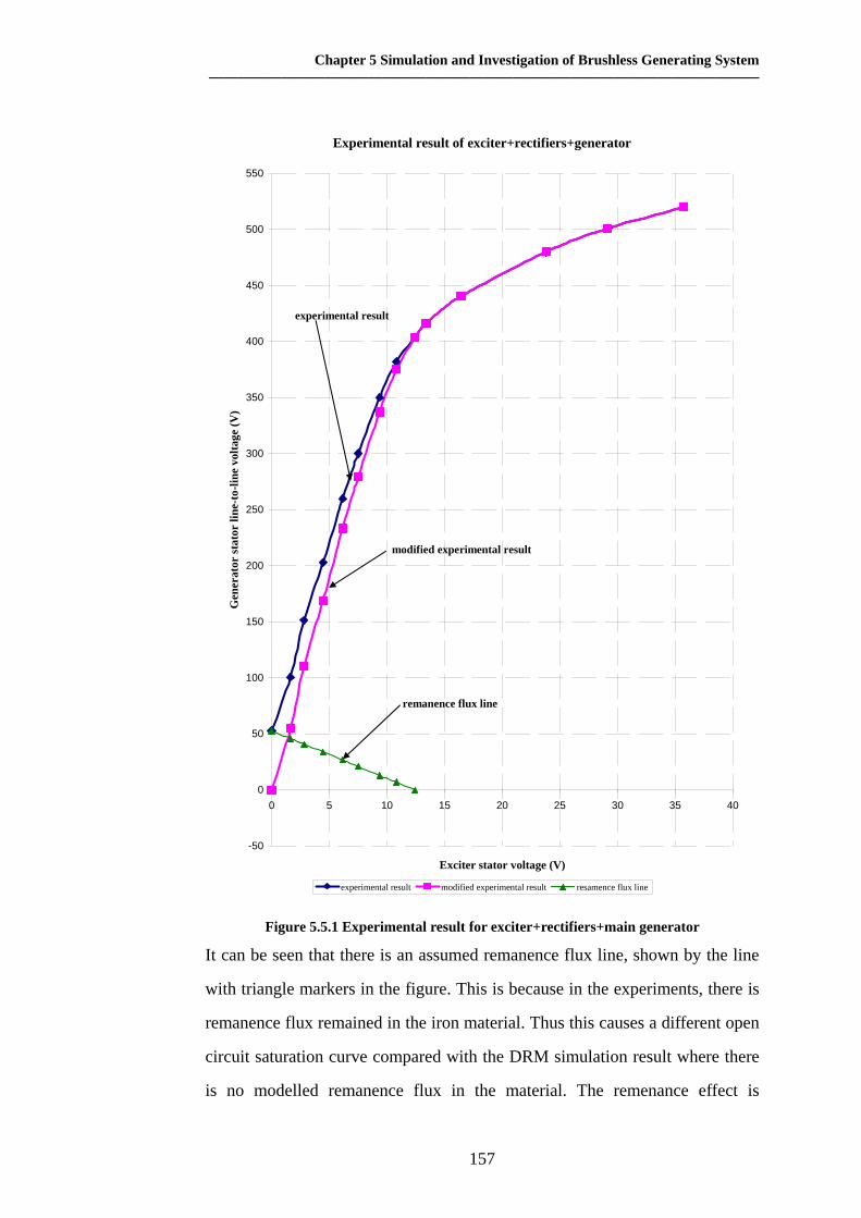
Chapter 5 Simulation and Investigation of Brushless Generating System ——————————————————————————————————————
157
Experimental result of exciter+rectifiers+generator
-50
0
50
100
150
200
250
300
350
400
450
500
550
0 5 10 15 20 25 30 35 40
Exciter stator voltage (V)
Gen
erat
or st
ator
line
-to-
line
volta
ge (V
)
experimental result modified experimental result resamence flux line
experimental result
modified experimental result
remanence flux line
Figure 5.5.1 Experimental result for exciter+rectifiers+main generator
It can be seen that there is an assumed remanence flux line, shown by the line
with triangle markers in the figure. This is because in the experiments, there is
remanence flux remained in the iron material. Thus this causes a different open
circuit saturation curve compared with the DRM simulation result where there
is no modelled remanence flux in the material. The remenance effect is

Chapter 5 Simulation and Investigation of Brushless Generating System ——————————————————————————————————————
158
particularly noticeable in the low voltage section of the saturation curve. The
small remanace in the exciter generate current in the field of the main generator.
The exciter magnetic circuit uses a different magnetic material to the main
generator and has in effect a shorter air gap thus maintaining the remanance
flux more easily. It can be seen from the results of chapter 4 that there is little
remanance effect in the generator itself.
The remanence flux line is derived by assuming that no remanence flux is
present at the working point, e.g. the rated voltage, and zero generated voltage
is assumed when the excitation voltage is zero. A linear variation of the
remanence voltage is assumed. A modified experimental result after
eliminating the remanence flux in the iron is shown in figure 5.5.1 by the line
with rectangular markers. The generated voltage now starts from zero when
there is no excitation. Now the comparison between this modified experimental
result and DRM result is shown in figure 5.5.2.

Chapter 5 Simulation and Investigation of Brushless Generating System ——————————————————————————————————————
159
Comparison of results from DRM with experimental result
0
50
100
150
200
250
300
350
400
450
500
550
0 5 10 15 20 25 30 35 40
Exciter stator voltage (V)
Gen
erat
or st
ator
line
-to-li
nevo
ltage
(V)
-4
-2
0
2
4
6
8
10
12
14
Err
or%
modified experimental result DRM_3 tip result error in percentage
modified experimental result
DRM simulation result
Error%
Figure 5.5.2 DRM simulation results in comparison to modified experimental results for open circuit testing
It can be seen from the result comparison in figure 5.5.2 that DRM result and
modified experimental result show perfect agreement in the region below
saturation. The bigger difference between the two results above the knee point
is due to the slightly different material that have been used in the DRM

Chapter 5 Simulation and Investigation of Brushless Generating System ——————————————————————————————————————
160
simulation and experiment, this is the same reason for the difference in the
open circuit test results in chapter 4.
5.6 AVR Controller Modelling
The DRM model of the exciter, rectifier and main generator have been
investigated and validated in the previous in this chapter. To model the
complete small brushless generating system, the excitation controller will now
be modelled. The design and implementation of a digital excitation controller
will be presented in this section, as well as the DRM simulations results.
5.6.1 Introduction
In a typical electrical power generation system, the excitation control system is
essential and a key component to the power system stability and controllability.
The functionality of the excitation control system in the structure of a power
generating system is to supply the field voltage to the main generator, as well
as to control the stability of the generating system. Normally, the excitation
control system comprises the Automatic Voltage Regulator (AVR) and the
Exciter a.c. generator, as shown in figure 5.6.1.
The first block in the middle row in figure 5.6.1 is a controller, which generates
the excitation voltage needed by the exciter stator based on the voltage error
between referenced voltage value and the main generator stator terminal
voltage value. The field voltage of the main generator is fed by the exciter
output through the rotating rectifiers.
The aim of the excitation system is to keep the stator terminal voltage of the
generating system equal to the reference value refV . There are power stabilizers
in figure 5.6.1. The aim of adding the power stabilizer is to add an additional
torque component to reduce the rotor oscillations following transients. This is
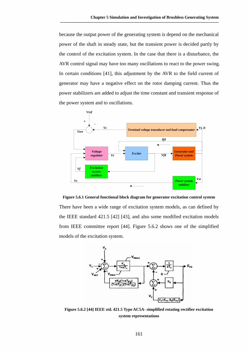
Chapter 5 Simulation and Investigation of Brushless Generating System ——————————————————————————————————————
161
because the output power of the generating system is depend on the mechanical
power of the shaft in steady state, but the transient power is decided partly by
the control of the excitation system. In the case that there is a disturbance, the
AVR control signal may have too many oscillations to react to the power swing.
In certain conditions [41], this adjustment by the AVR to the field current of
generator may have a negative effect on the rotor damping current. Thus the
power stabilizers are added to adjust the time constant and transient response of
the power system and to oscillations.
Voltageregulator Exciter Generator and
Power system
Excitationsystem
stabilizer
Power systemstablizer
Terminal voltage transducer and load compensator
+ _
Vref
VcVerr
Vf
Vs
Vr Vfd
Vst
Ifd
Vt, It
Figure 5.6.1 General functional block diagram for generator excitation control system
There have been a wide range of excitation system models, as can defined by
the IEEE standard 421.5 [42] [43], and also some modified excitation models
from IEEE committee report [44]. Figure 5.6.2 shows one of the simplified
models of the excitation system.
Figure 5.6.2 [44] IEEE std. 421.5 Type AC5A- simplified rotating rectifier excitation
system representations

Chapter 5 Simulation and Investigation of Brushless Generating System ——————————————————————————————————————
162
A practical excitation control system for the small brushless salient pole
generating system described in the thesis is shown in the Simulink diagram of
figure 5.6.3 [45].
Figure 5.6.3 [45] The practical excitation system model for the generating system in the
thesis
In figure 5.6.3, the automatic voltage regulator, exciter, generator and the
stabilizer have all been modelled. There are other models that have been used
for small salient pole generators [42].
However, for the brushless generating system simulations in this thesis, only
the simplest excitation controls will be applied because the addition of the
control is only to demonstrate that a full system may be modelled using the
DRM method.
The structure of the whole small brushless synchronous generating system to
be simulated in this thesis is shown in figure 5.6.4. A PID (Proportional,
Integral and Derivative) controller was designed and implemented as the
automatic voltage regulator. The DRM model for the exciter, rotating rectifiers
and the main have been described and validated in previous sections. This
section will concentrate on the controller design and implementation.
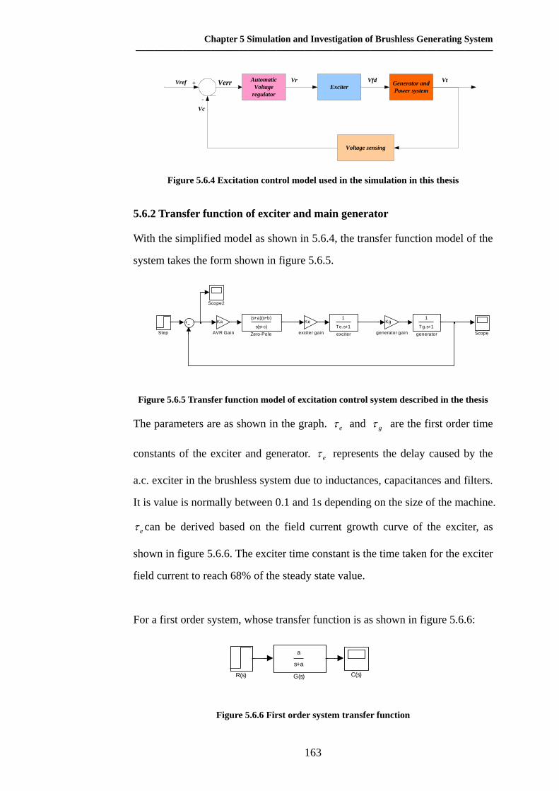
Chapter 5 Simulation and Investigation of Brushless Generating System ——————————————————————————————————————
163
AutomaticVoltage
regulatorExciter Generator and
Power system
Voltage sensing
+Vref Verr
-Vc
Vr Vfd Vt
Figure 5.6.4 Excitation control model used in the simulation in this thesis
5.6.2 Transfer function of exciter and main generator
With the simplified model as shown in 5.6.4, the transfer function model of the
system takes the form shown in figure 5.6.5.
Kg
generator gain
1
Tg.s+1generator
Ke
exciter gain
1
Te.s+1exciter
(s+a)(s+b)
s(s+c)Zero-PoleStep
Scope2
Scope
Ka
AVR Gain
Figure 5.6.5 Transfer function model of excitation control system described in the thesis
The parameters are as shown in the graph. eτ and gτ are the first order time
constants of the exciter and generator. eτ represents the delay caused by the
a.c. exciter in the brushless system due to inductances, capacitances and filters.
It is value is normally between 0.1 and 1s depending on the size of the machine.
eτ can be derived based on the field current growth curve of the exciter, as
shown in figure 5.6.6. The exciter time constant is the time taken for the exciter
field current to reach 68% of the steady state value.
For a first order system, whose transfer function is as shown in figure 5.6.6:
R(s)
a
s+a
G(s) C(s)
Figure 5.6.6 First order system transfer function

Chapter 5 Simulation and Investigation of Brushless Generating System ——————————————————————————————————————
164
For a step input ssR /1)( = , the step response is given by:
sasasGsRsC 1)()()( ⋅+
== (5.6.1)
the step response in time domain is:
atnf etctctc −−=+= 1)()()( (5.6.2)
time constant for first order system is defined as: a1
=τ , when:
( ) ininat
atat
ccetc 632.01)(/1/1
=−==
−=
(5.6.3)
Where )(tc is system output signal, and inc is system input value. Thus, the time
constant for the exciter could be derived given the field rising curve in exciter
stator, shown in figure 5.6.6.
Exciter field current
0
0.1
0.2
0.3
0.4
0.5
0.6
0.7
0 0.03 0.06 0.09 0.12 0.15 0.18 0.21 0.24 0.27 0.3 0.33 0.36 0.39 0.42 0.45 0.48
Time(s)
Stat
or c
urre
nt(A
)
Steady state value of field current =0.61A
0.632*steady state value of field current=0.38552
field time constant=the time when field current reach 0.632*steady state value = 0.0778
Figure 5.6.6 Deriving the field time constant of exciter
And eτ is: se 0778.0=τ .
For the time constant of the generator, gτ represents any delay caused by the
generator main field winding due to its inductances (L/R time constants). Its
value is dependent on the machine that the AVR is connected to and should be
taken from available data and generator models. Its value is normally between

Chapter 5 Simulation and Investigation of Brushless Generating System ——————————————————————————————————————
165
0.25 and 2s depending on the size of machine. Using the same method in
deriving the time constant for the exciter, gτ could be derived. The rising of
field current of generator is shown in figure 5.6.7.
generator field current
0
1
2
3
4
5
6
7
8
9
10
11
12
13
14
15
0 0.2 0.4 0.6 0.8 1 1.2 1.4 1.6 1.8 2 2.2 2.4 2.6 2.8 3 3.2 3.4 3.6 3.8 4
time(s)
Cur
rent
(Am
ps)
Steady state value of field current =13.67
0.632*steady state value of field current = 8.64
field time constant= the time when field current reach 0.632*steady state value=0.9533
Figure 5.6.7 Deriving the field time constant of main generator
And gτ is: sg 9533.0=τ
As for the loop gain, including eK and gK , based on the experimental data
from the sponsor, the gain from the field voltage to stator terminal per phase
voltage is:
73139619.18==⋅voltagefieldstatorexciter
voltagephasestatorgeneratorKK ge (5.6.4)
In the feedback loop where the generator output voltage is sensed, the
three-phase stator voltage value has to be transformed to a single value, in
order to compare with the single reference value. In a practical AVR controller
or complicated models, shown in figure 5.6.3, this is done by the voltage
detector. Here in the simulations in this thesis, the stator terminal voltage
needed by the controller was derived numerically by transformation using the
commutator and three phase to two phase (α , β ) transformations [32]. Thus
the delay caused by the voltage detection was neglected.

Chapter 5 Simulation and Investigation of Brushless Generating System ——————————————————————————————————————
166
The transformation in DRM program from the three phase (A, B, C) magnitude
value to two phase ( βα , ) value is as shown below:
⎥⎥⎥
⎦
⎤
⎢⎢⎢
⎣
⎡
⎥⎦
⎤⎢⎣
⎡−−−
⋅=⎥⎦
⎤⎢⎣
⎡
c
b
a
xxx
xx
232/1
2/32/1
01
32
β
α (5.6.5)
where x represents the stator voltage magnitude sv .
The transformations yield the peak value of the a.c. voltage multiplied by23 .
The commutator transform converts the two phase a.c. representation into two
phase direct voltage representation on the d and q axes and the peak value is
extracted from by squaring these components, adding them and taking the
square root. Thus 223
32 ⋅=K =1.732.
Then this magnitude will be fed back to the controller, as shown in figure 5.6.8
below.
genset output voltage, per phase
Kg
generator gain
1
Tg.s+1generator
Ke
exciter gain
1
Te.s+1exciter
error
(s+a)(s+b)
s(s+c)Zero-PoleStep Scope
Ka
AVR Gain
K32
3-2 voltage transform
Figure 5.6.8 Simulated voltage sensing in DRM simulation
Considering all the gains included in the loop, the transfer function for the
exciter and the main generator finally becomes:
( )( ) ( )( )048987727.185347044.124431167.437
11)( 32
++=
++=
ssssKKK
sGge
gep ττ
(5.6.6)

Chapter 5 Simulation and Investigation of Brushless Generating System ——————————————————————————————————————
167
5.6.3 Design of PID controller
A typical structure of a digital PID controller [46] [47] [48] is shown in figure
5.6.9.
Kp
Ki/s
KDs/(1+Tfs)
Vref
Vc
+
-
Verr+
+
+
Vr
Figure 5.6.9 Digital PID controller used in this thesis
Where, pK is the proportional gain; iK is the integral gain; DK is the
derivative gain; fT is the low pass filter time constant. And the relationship
between these coefficients and the integral time constant, derivative time
constant are:
i
pi
KK
τ= (5.6.7)
DpD KK τ= (5.6.8)
and the digital PID controller’s transfer function is in the form of:
)1(
)()()(
2
f
fi
p
i
p
f
p
f
dpp
c
Tss
TK
sK
TK
sT
KK
sG+
++++
=ττ
τ
(5.6.9)
Using the controller design technique in continuous domain, the root locus
controller design method is used. Intuitively, two zeros in the controller will be
added close to poles of the exciter and the main generator [46]. And another
pole in the controller is added to ensure the root locus passes through the
design point. Details of the controller design procedure for the brushless
generating system described in this thesis can be found in Appendix 5. The
Chapter 5 Simulation and Investigation of Brushless Generating System ——————————————————————————————————————
168
controller is designed to have a damping ratio 8.0=ζ , to guarantee that there is
not a large overshoot, and the natural frequency is Hzn 25=ω .
Designed controller’s transfer function of the controller takes the form:
( )( ))100(
419611.5)(+
++=
sssssGc (5.6.10)
where for digital PID controller, 259.1=pK , 3.0=iτ , 035.0=Dτ ,
01.0=fT .
In order to use this continuous PID controller in computer code, Z
transformations have to be made. The transfer function after Z transformations
is:
)2()()1(
)2()()())1(2()()(**
****
TtVeTtVe
TtEATeCeBTtEATeCBtEKtV
raT
raT
aTaTaTcr
−−−++
−−++−−++−=−−
−−−
(5.6.11)
where )(* tV r is the output voltage of the controller, )(* tE is the error input for
the controller,
661.5=cK
100419 ⋅⋅
= cKA
CKB c −=
( )( )100
419 AKC c −+=
100=a (5.6.12)
sample time used in DRM simulation is 0.01s, and the details of the controller
design can be found in Appendix 5.
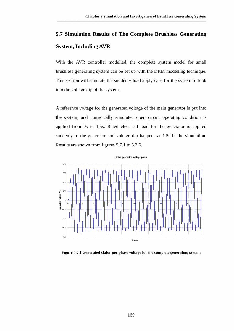
Chapter 5 Simulation and Investigation of Brushless Generating System ——————————————————————————————————————
169
5.7 Simulation Results of The Complete Brushless Generating
System, Including AVR
With the AVR controller modelled, the complete system model for small
brushless generating system can be set up with the DRM modelling technique.
This section will simulate the suddenly load apply case for the system to look
into the voltage dip of the system.
A reference voltage for the generated voltage of the main generator is put into
the system, and numerically simulated open circuit operating condition is
applied from 0s to 1.5s. Rated electrical load for the generator is applied
suddenly to the generator and voltage dip happens at 1.5s in the simulation.
Results are shown from figures 5.7.1 to 5.7.6.
Stator generated voltage/phase
-400
-300
-200
-100
0
100
200
300
400
0 0.1 0.2 0.3 0.4 0.5 0.6 0.7 0.8 0.9 1
Time(s)
Gen
erat
ed v
olta
ge (V
)
Figure 5.7.1 Generated stator per phase voltage for the complete generating system

Chapter 5 Simulation and Investigation of Brushless Generating System ——————————————————————————————————————
170
System error
-100
-50
0
50
100
150
200
250
300
350
0 0.1 0.2 0.3 0.4 0.5 0.6 0.7 0.8 0.9 1
Time(s)
Err
or (V
olts
)
Figure 5.7.2 Error between reference voltage value and feedback voltage value
AVR controller output
-500
0
500
1000
1500
2000
2500
0 0.1 0.2 0.3 0.4 0.5 0.6 0.7 0.8 0.9 1
Tims(s)
AV
R o
utpu
t vol
tage
(Vol
ts)
Figure 5.7.3 AVR controller output value
Figures 5.7.1-5.7.3 show the generated main generator stator voltage waveform,
the system error and AVR controller output waveform in a numerically
simulated open circuit case. It can be seen that the system’s overshoot is small
and the response time is fast.

Chapter 5 Simulation and Investigation of Brushless Generating System ——————————————————————————————————————
171
Stator generated voltage/phase
-400
-300
-200
-100
0
100
200
300
400
1 1.2 1.4 1.6 1.8 2 2.2 2.4 2.6 2.8 3
Time(s)
Gen
erat
ed v
olta
ge (V
)
Figure 5.7.4 Generated stator per phase voltage for the complete generating system
during a voltage dip
System error
-100
-50
0
50
100
150
200
250
300
350
1 1.2 1.4 1.6 1.8 2 2.2 2.4 2.6 2.8 3
Time(s)
Err
or (V
olts
)
Figure 5.7.5 Error between reference voltage value and feedback value during a voltage
dip
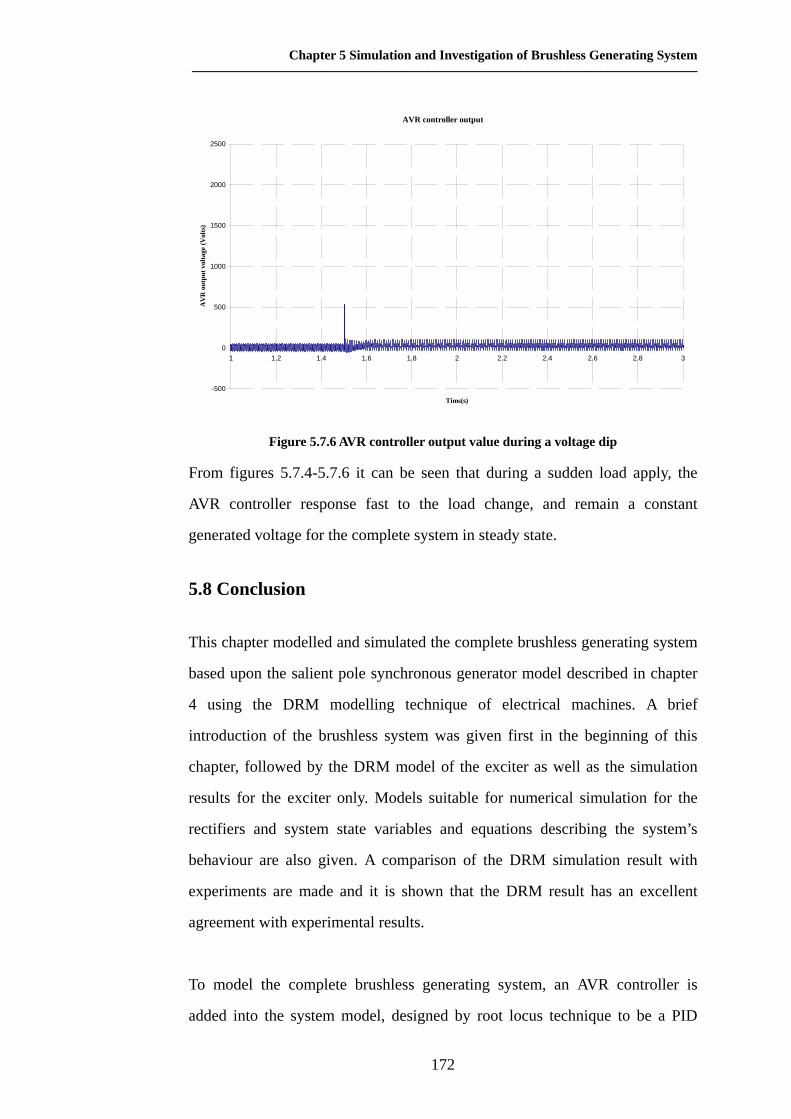
Chapter 5 Simulation and Investigation of Brushless Generating System ——————————————————————————————————————
172
AVR controller output
-500
0
500
1000
1500
2000
2500
1 1.2 1.4 1.6 1.8 2 2.2 2.4 2.6 2.8 3
Tims(s)
AV
R o
utpu
t vol
tage
(Vol
ts)
Figure 5.7.6 AVR controller output value during a voltage dip
From figures 5.7.4-5.7.6 it can be seen that during a sudden load apply, the
AVR controller response fast to the load change, and remain a constant
generated voltage for the complete system in steady state.
5.8 Conclusion
This chapter modelled and simulated the complete brushless generating system
based upon the salient pole synchronous generator model described in chapter
4 using the DRM modelling technique of electrical machines. A brief
introduction of the brushless system was given first in the beginning of this
chapter, followed by the DRM model of the exciter as well as the simulation
results for the exciter only. Models suitable for numerical simulation for the
rectifiers and system state variables and equations describing the system’s
behaviour are also given. A comparison of the DRM simulation result with
experiments are made and it is shown that the DRM result has an excellent
agreement with experimental results.
To model the complete brushless generating system, an AVR controller is
added into the system model, designed by root locus technique to be a PID

Chapter 5 Simulation and Investigation of Brushless Generating System ——————————————————————————————————————
173
controller. DRM simulations incorporating controls for the complete system are
made, and results show that the AVR works fine in a voltage dip condition.

Chapter 6 Multiple Machine System-Cascaded DFIM Simulation
174
CHAPTER 6 MULTIPLE MACHINE SYSTEM-
CASCADED DOUBLY FED INDUCTION MACHINE
SIMULATION
6.1 Introduction
In previous chapters, DRM modelling of small salient-pole synchronous
generator and the modelling of brushless generating system, including exciter,
automatic voltage regulator, rotating rectifiers and the generator, has been
investigated and validated. It has been shown that DRM modelling of an
electrical machine is an effective and flexible method, and its application could
be further extended to the simulation and investigation of multi-machine
systems. Such a system is a cascaded doubly fed induction generator for use in
wind energy generation.
In this chapter, the multiple-machine, system-cascaded, doubly-fed, induction
generator, which is a research interest in the field of wind energy generation in
recent years, will be modelled and simulated by the Dynamic Reluctance
Method. Simulation results in the respect of power flow and frequency changes
in the cascaded doubly fed induction machine system will be discussed. In the
beginning of this chapter, some simple introduction of the application field of
cascaded machine is presented.
Renewable energy, such as wind energy, hydro energy, geothermal energy and
solar energy invokes great interest these years, due to the increasing concerns
for the environment and finite hydrocarbon resources. These renewable
energies are clean energy suitable for the next century, and have minimum
environmental impact.
Among these energy sources, wind and hydro energy are the most widely
adopted renewable approaches for industrial electricity generation applications.
For example, more than 20% of electricity consumption in the west of

Chapter 6 Multiple Machine System-Cascaded DFIM Simulation
175
Denmark is provided by wind energy [49], and their utilization is felt to be
very promising to help provide the future energy requirements. Offshore and
remote regions offer great potential for exploiting wind energy. Research into
cost effective solutions for such locations is currently being carried out.
Many wind energy generation systems have been proposed over the years [16]
[50] [51]. Current maximum power ratings are around 5 MW [52] [53] but are
increasing with time due to developments in technology. From the electrical
machine point of view, wind energy generators could be classified as
asynchronous generator, synchronous generators and even reluctance rotor
machines. Asynchronous generators are most common for a small rating wind
generating system under 2MW, and direct-driven permanent magnet
synchronous machines are preferred for a larger rating.
Many types of wind generators have been proposed and validated, among them,
the common type of wind generating system can be shown in figure 6.1.
Figure 6.1.1 Fixed speed wind generating system
Figure 6.1 shows a fixed speed wind generating system, with capacitor bank
staying on the stator side, between the grid and the generator, which is a widely
used commercial choice due to its simplicity in design and low cost. The
machine has normally two set of stator windings with different pole numbers,
thus implement fixed frequency current at two different shaft speed. Although
this kind of fixed speed system is reliable and simple, it limits the power output
of the wind generating system because of the capacitor bank. Efficiency in
power extraction from the wind is critical in defining the economic limit of
application of a wind turbine.
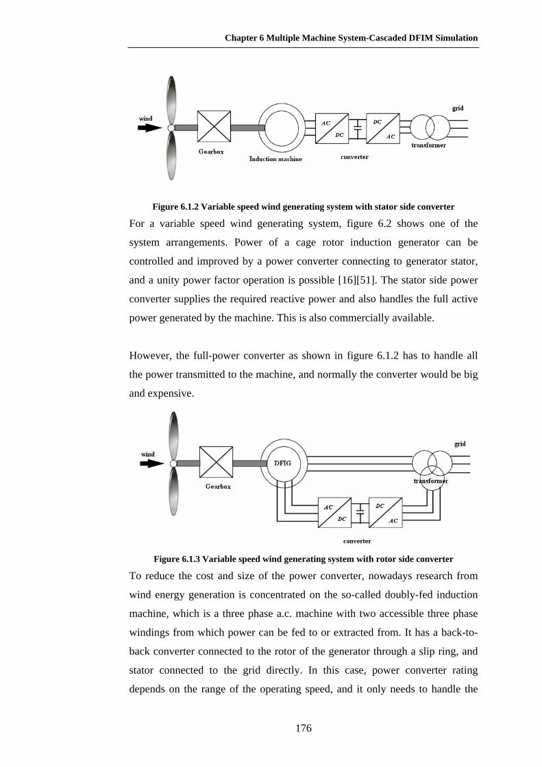
Chapter 6 Multiple Machine System-Cascaded DFIM Simulation
176
Figure 6.1.2 Variable speed wind generating system with stator side converter
For a variable speed wind generating system, figure 6.2 shows one of the
system arrangements. Power of a cage rotor induction generator can be
controlled and improved by a power converter connecting to generator stator,
and a unity power factor operation is possible [16][51]. The stator side power
converter supplies the required reactive power and also handles the full active
power generated by the machine. This is also commercially available.
However, the full-power converter as shown in figure 6.1.2 has to handle all
the power transmitted to the machine, and normally the converter would be big
and expensive.
Figure 6.1.3 Variable speed wind generating system with rotor side converter
To reduce the cost and size of the power converter, nowadays research from
wind energy generation is concentrated on the so-called doubly-fed induction
machine, which is a three phase a.c. machine with two accessible three phase
windings from which power can be fed to or extracted from. It has a back-to-
back converter connected to the rotor of the generator through a slip ring, and
stator connected to the grid directly. In this case, power converter rating
depends on the range of the operating speed, and it only needs to handle the

Chapter 6 Multiple Machine System-Cascaded DFIM Simulation
177
slip power of the machine, thus the size and cost of the whole system are
reduced substantially. But, maintenance cost would be high due to the presence
of slip rings and brushes.
Viable alternatives for the doubly fed induction machine have been proposed to
get rid of the slip rings and brushes, which are called brushless, doubly-fed,
induction machines [51]. The cascaded doubly fed induction machine, as
referred to by Hopfernsperger [20] [54], is one of the alternatives.
6.2 Cascaded Doubly-fed Induction Machine in Wind Energy
Technology
A single doubly fed induction machine (SDFM) [54], has the topology as
shown in figure 6.1.3. The stator winding of a wound rotor induction machine
is connected to a stiff voltage supply and the rotor winding is connected to a bi-
directional power converter. The main drawback of this kind of arrangement is
the slip ring brushes combination [20]. The brushless doubly fed induction
machine is designed to take the slip ring and brushes out of the machine system.
Cascaded doubly fed induction machine (CDFM) is one of the brushless
arrangements.
Cascade doubly fed induction machine is the arrangement that connecting two
wound rotor induction machine together, mechanically and electrically. The
two machines stay on the same shaft, and one stator winding is connected to
the grid, while the other stator winding is connected to the power converter. Its
structure is shown in figure 6.2.1. Since the two rotors have a stiff mechanical
coupling no brushes are need for the slip ring connection.

Chapter 6 Multiple Machine System-Cascaded DFIM Simulation
178
Figure 6.2.1 Cascaded doubly-fed induction machine (CDFM)
Excitation to the rotor of machine A in figure 6.2.1 is transferred between the
stator of the induction machine that is connected to the converter (machine B)
to the machine that is generating (machine A).
There are two kinds of electrical connection for the cascade doubly fed
induction machine: positive phase sequence connection and negative phase
sequence connection. Positive phase sequence results by connecting the rotor
windings together with the same phase sequence. And negative phase sequence
result by swapping the phase sequence on side 3 of machine B. If the two
machines mechanical connected in series, as the case in figure 6.2.1, with a
negative phase sequence electrical connection, the rotating flux field on the two
rotor would be opposite relative to the rotor, and the developed toque for
machine A and B are co-acting in this negative connection case. However, if
the rotors are connected in positive connection electrically, the rotating fields
have the same rotating direction. The developed torque is counter-acting for
this negative sequence connection [54]. Therefore, with the two machines
connected in series mechanically, only the negative phase sequence connection
of real importance is under consideration in the thesis.
But, things would be different for a back-to-back machine arrangement [54]. A
positive phase sequence would be appropriate for back-to-back connected
cascaded machines, to generate co-acting torque on the two machines and also
generate opposite direction rotor rotating flux fields relative to the rotor. In this

Chapter 6 Multiple Machine System-Cascaded DFIM Simulation
179
case, the positive phase sequence is of importance and could be generating the
current with the frequency that is needed.
As mentioned in reference [20][54][55], the resulting frequency relationship
for a CDFM machine connected in series between machine stator current and
rotor currents is:
41 )( ffppf mBA −+= (6.2.1)
where 1f and 4f are the stator side frequencies in side 1 and side 4 for machine
A and machine B in figure 6.2.1. Ap and Bp are the number of pole pairs in the
two machines, mf is the mechanical rotor frequency. In the 4 pole, cascade
machine system described in this thesis, the stator of machine A is connected to
the 50Hz electric grid. Side 2 and 3 are identical apart from the phases due to
the negative phase sequence connections. The CDFM machine reaches the
synchronous point of machine A at 750 rpm, while 032 == ff . The
relationship of these frequencies is shown in figure 6.2.2.
Frequency relationship in cascaded doubly fed induction machine (series connection)
-60
-40
-20
0
20
40
60
0 100 200 300 400 500 600 700 800 900 1000
Shaft speed (rpm)
Freq
uenc
y (H
z)
f1 f2 f3 f4
f1: grid side stator frequency
f4: converter side stator frequency
f2: machine A rotor frequency
f3: machine B rotor frequency
Figure 6.2.2 Frequency relationship in series connected cascaded doubly fed induction
machines As seen from figure 6.2.2, in synchronous speed, which is 750rpm in the case
that is considered here, the converter stator side 4 frequency is 0, d.c. voltage is
supplied to the converter side machine B, and 50Hz current should come out
from the grid side stator in machine A. In other shaft speed cases, where shaft

Chapter 6 Multiple Machine System-Cascaded DFIM Simulation
180
speed is above or below the synchronous speed, the frequency on stator side of
grid side machine A would be changed to negative or positive according to the
frequency characteristic given in figure 6.2.2. In another word, from the power
pint of view, electric power flow into the cascaded doubly fed induction
machine system with a shaft speed lower than synchronous speed, and flow out
of the system in the higher shaft speed than synchronous speed, when 4f is
positive. P.s. assume power flowing into the cascaded machine system is
negative in sign, power flowing into the grid is positive in sign.
In later simulations of cascaded machine system presented in this thesis, two
typical cases: shaft speed to be 550 rpm and 950 rpm, will be considered and
simulated. The frequencies in the stator terminals, rotor windings, as well as
the powers that are flowing in or out of the system, will be investigated.
However, the DRM modelling of cascaded machines will be described next.
The advantage of DRM modelling is that saturation, skew, phase belt
harmonics and tooth harmonics can all be examined in detail and their
influence on system performance assessed. These practical issues of
implementing a large system might well cause problems for the control and
power electronic components. It has already been demonstrated in chapter 5
that incorporation of these elements into DRM simulations can be readily
achieved. It is thus possible to simulate in detail the complete wind energy
recovery system and examine design changes to obtain a viable solution quite
quickly. The following work however concentrates solely on the electrical
machine aspects.
6.3 DRM Model of Cascaded Doubly-fed Induction Machine
Detailed DRM model of induction machines has been introduced and improved
in chapter 2 and 3 separately. Here in this chapter, the concentration would be
the electrical and mechanical connection of the two cascaded machines.

Chapter 6 Multiple Machine System-Cascaded DFIM Simulation
181
Figure 6.3.1 Electrical and mechanical connection diagram of cascaded machine system
As is shown in figure 6.3.1, machine A and machine B are connected on the
same shaft, and in series sequence mechanically, different from the back-to-
back mechanical connection used in reference [54]. With this mechanical
connection, in order to generate constant frequency under different shaft speed,
the negative phase sequence electrical connection between the two rotors has to
be utilized, as mentioned in previous section in this chapter. In figure 6.3.1,
phase B and phase C of the rotors for the two induction machine have been
swapped, for a negative phase sequence.
The electrical loop connection between the connected rotors in the two
machines is shown in figure 6.3.2. The outer loop, loop B, is the electrical loop
that connects phase B in machine B and phase C in machine A. The inner loop,
loop C, is the electrical loop that connects phase C in machine B and phase B
in machine A.
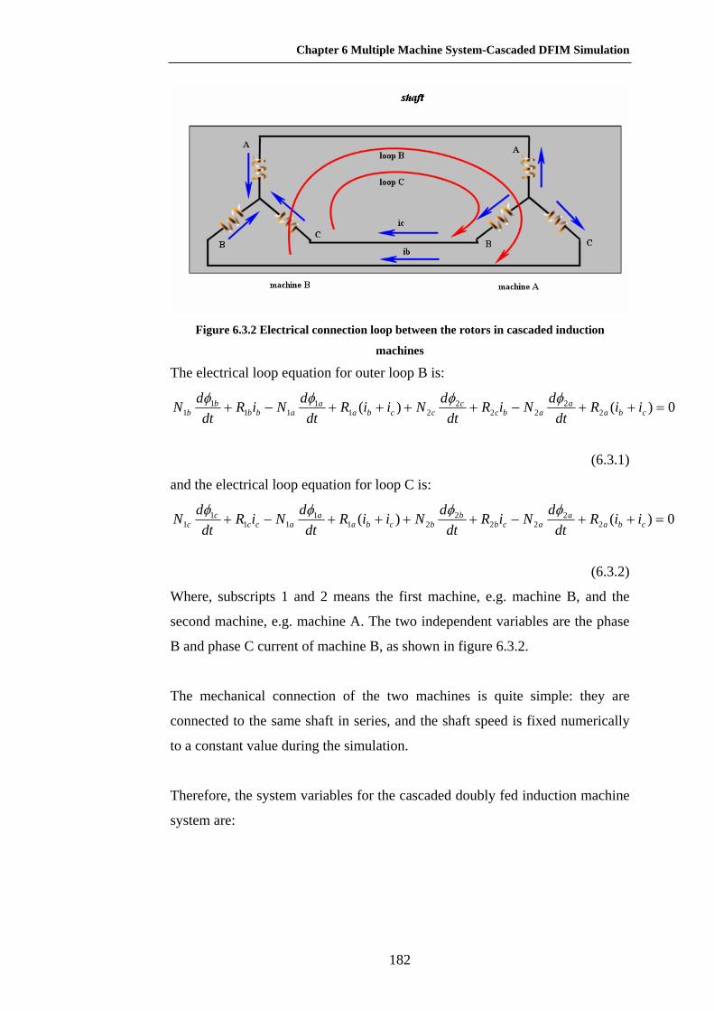
Chapter 6 Multiple Machine System-Cascaded DFIM Simulation
182
Figure 6.3.2 Electrical connection loop between the rotors in cascaded induction
machines
The electrical loop equation for outer loop B is:
0)()( 22
222
211
111
1 =++−++++−+ cbaa
abcc
ccbaa
abbb
b iiRdt
dNiRdt
dNiiRdt
dNiRdt
dN φφφφ
(6.3.1)
and the electrical loop equation for loop C is:
0)()( 22
222
211
111
1 =++−++++−+ cbaa
acbb
bcbaa
accc
c iiRdt
dNiRdt
dNiiRdt
dNiRdt
dN φφφφ
(6.3.2)
Where, subscripts 1 and 2 means the first machine, e.g. machine B, and the
second machine, e.g. machine A. The two independent variables are the phase
B and phase C current of machine B, as shown in figure 6.3.2.
The mechanical connection of the two machines is quite simple: they are
connected to the same shaft in series, and the shaft speed is fixed numerically
to a constant value during the simulation.
Therefore, the system variables for the cascaded doubly fed induction machine
system are:

Chapter 6 Multiple Machine System-Cascaded DFIM Simulation
183
⎟⎟⎟⎟⎟⎟⎟⎟⎟⎟⎟⎟⎟⎟⎟⎟⎟⎟⎟
⎠
⎞
⎜⎜⎜⎜⎜⎜⎜⎜⎜⎜⎜⎜⎜⎜⎜⎜⎜⎜⎜
⎝
⎛
−
−
=
current C phasestator A machinecurrent B phasestator A machine
Potentialmmf1N nodeA machine
Potentialmmf0 nodeA machineangle rotatingrotor
current rotorcommon machines twocurrent rotorcommon machines two
currentCphasestatorB machinecurrentBphasestatorB machine
potentialmmf1NnodeB machine
potentialmmf0nodeB machine
A
B
L
K
c
b
ii
x (6.3.4)
and the equations that describe the cascade machine system are:
⎟⎟⎟⎟⎟⎟⎟⎟⎟⎟⎟⎟⎟⎟⎟⎟⎟⎟⎟
⎠
⎞
⎜⎜⎜⎜⎜⎜⎜⎜⎜⎜⎜⎜⎜⎜⎜⎜⎜⎜⎜
⎝
⎛
−
−
=
equation electricalV phaseA machineequaiton electricalV phaseA machine
1Nnodeat A machineinflux ofonconservati
0nodeat A machineinflux ofonconservatiequation speed
C loop 6.3.2,equaitonB loop 6.3.1,equation
equation electricalV phase B machineequaiton electricalV phase B machine
1Nnodeat B machineinflux ofonconservati
0nodeat B machineinflux ofonconservati
AC
AB
A
AC
AB
B
L
L
F(x) (6.3.5)
Having these system equations and system variables, the system state could be
solved by using the globally convergent Newton-Raphson method mentioned
in chapter 3. The simulation result will be shown in next section, and also
some discussion of the results.
6.4 Simulation Results
In this section, the DRM simulation results of the cascaded doubly fed
induction machine system will be discussed and investigated. Currents and
power flow between the machines and terminals will be shown.

Chapter 6 Multiple Machine System-Cascaded DFIM Simulation
184
Three operation circumstances of the system will be considered: sub-
synchronous speed, synchronous speed and super-synchronous speed. The
machine system is two identical induction machines, with 4 poles each with 48
stator slots and 36 rotor slots. The coil pitch of the machine stator winding is
10 and 8 for the rotor winding. Further details can be found in appendix 2.
Synchronous speed of this system is 750 rpm, as stated in the previous section.
The super-synchronous operation case 950 rpm will be considered as a typical
case in this section, while sub-synchronous case would be 550 rpm. The
operation range of this turbine would be 0.73 p.u. to 1.26 p.u.. Rated load at
1.0pf is applied to the grid side of the machine system, and the load is star
connected.
6.4.1 Sub-synchronous speed, shaft speed - 550 rpm
When the shaft is rotating at sub-synchronous speed, a low frequency a.c
voltage source is applied to the stator side 4 of machine B, through the
converter. Normally in a controlled cascaded doubly fed induction machine
system, the frequency and the applied voltage are controlled by the converter.
However, in the discussion and simulation in the thesis, a voltage source with
fixed frequency and voltage value, which is decided by the shaft speed, is
applied to converter side stator directly, and no control details will be discussed
here. Frequency relations in sub-synchronous speed, which is 550 rpm, can be
seen in figure 6.4.1.

Chapter 6 Multiple Machine System-Cascaded DFIM Simulation
185
Figure 6.4.1 Frequency relations in sub-synchronous speed – 550 rpm for CDFM
As can be seen in figure 6.4.1, 13.3 Hz frequency stator voltage source is
applied to the converter side stator, e.g. side 4, thus the stator flux field rotating
in a counter-clockwise direction. This frequency is determined by the shaft
speed (electrical) with respect to the synchronous speed of the cascaded
machine system. The desired generation frequency is 50 Hz, which comes out
of side 1 of machine A, considering the shaft speed is sub-synchronous speed,
thus the slip frequency should be supplied by the converter. Thus, current
frequency for side 4 in machine B should be HzHz 3.1350750
)550750(=⋅
− .
In order to generate a steady torque in electrical machines, the stator flux field
and rotor flux field have to remain stationary with respect to each other, thus
the resultant rotor flux field rotating speed and direction has to be the same
with that of stator. In machine B, rotor is sitting on the shaft, which rotates at
the electrical frequency Hz33.18605502
=⋅ (each induction machine has 2 pole
pairs), and it is opposite to rotation of stator flux field. Thus the rotor flux field
rotation direction with respect to the shaft should be counter-clockwise and its
frequency is Hz67.3133.1333.18 =+ . Due to the negative phase sequence

Chapter 6 Multiple Machine System-Cascaded DFIM Simulation
186
connection between the two rotors of the CDFM system, rotor flux field
rotation direction in machine A is clockwise, which is the same direction with
the shaft rotation, as shown in figure 6.4.1. To remain the flux field in stator
and rotor to be the same in machine A, stator flux field frequency will be the
sum of the electrical rotation frequency of the shaft, which is 18.33Hz, and the
rotor flux field rotating frequency with respect to the shaft in machine A, which
is 31.67Hz. Thus, the generated stator flux field rotation frequency is
18.33Hz+31.67Hz=50Hz.
Figures 6.4.2-6.4.4 show the stator and rotor current waveforms in machine A
and machine B for CDFM system in sub-synchronous speed.
converter side stator (machine B) current@ 550rpm
-50
-40
-30
-20
-10
0
10
20
30
40
0 0.1 0.2 0.3 0.4 0.5 0.6 0.7
Time (s)
Mac
hine
B st
ator
cur
rent
(Am
ps)
Figure 6.4.2 Converter side (side 4) induction machine stator current waveform
Current frequency in figure 6.4.2 is 13.3 Hz, as what is expected according to
the analysis in previous context.
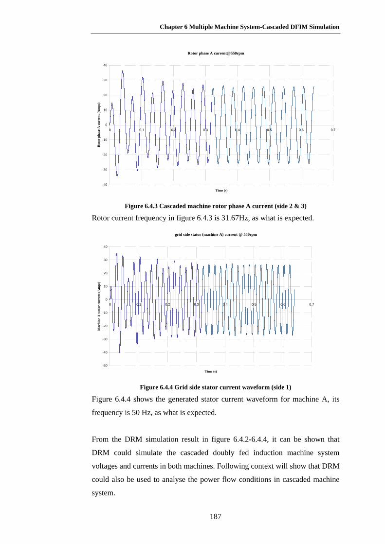
Chapter 6 Multiple Machine System-Cascaded DFIM Simulation
187
Rotor phase A current@550rpm
-40
-30
-20
-10
0
10
20
30
40
0 0.1 0.2 0.3 0.4 0.5 0.6 0.7
Time (s)
Rot
or p
hase
A c
urre
nt (A
mps
)
Figure 6.4.3 Cascaded machine rotor phase A current (side 2 & 3)
Rotor current frequency in figure 6.4.3 is 31.67Hz, as what is expected.
grid side stator (machine A) current @ 550rpm
-50
-40
-30
-20
-10
0
10
20
30
40
0 0.1 0.2 0.3 0.4 0.5 0.6 0.7
Time (s)
Mac
hine
A st
ator
cur
rent
(Am
ps)
Figure 6.4.4 Grid side stator current waveform (side 1)
Figure 6.4.4 shows the generated stator current waveform for machine A, its
frequency is 50 Hz, as what is expected.
From the DRM simulation result in figure 6.4.2-6.4.4, it can be shown that
DRM could simulate the cascaded doubly fed induction machine system
voltages and currents in both machines. Following context will show that DRM
could also be used to analyse the power flow conditions in cascaded machine
system.

Chapter 6 Multiple Machine System-Cascaded DFIM Simulation
188
The power flow conditions in sub-synchronous speed for CDFM are shown in
figure 6.4.5.
Figure 6.4.5 Power flow condition in sub-synchronous speed
Mechanical power flow into the cascaded doubly induction machine system
through the shaft, and shaft speed is below the synchronous speed in this sub-
synchronous speed case. Because the shaft speed is lower than the synchronous
speed, converter electrical power will flow into the cascaded machine system,
as shown in figure 6.4.5. Power relations for the cascaded machine system
speed condition would be:
losselectricalgeneratedelectricalconvertermech PPPP ++= (6.4.1)
In the sub-synchronous speed case, converter electrical power would be
negative (assume power flowing into the cascaded machine system and power
loss is negative in sign), and generated electrical power in side 1 would be
positive (assume power flowing into the grid is positive in sign). Power flow
simulation by DRM method is shown in figure 6.4.6.
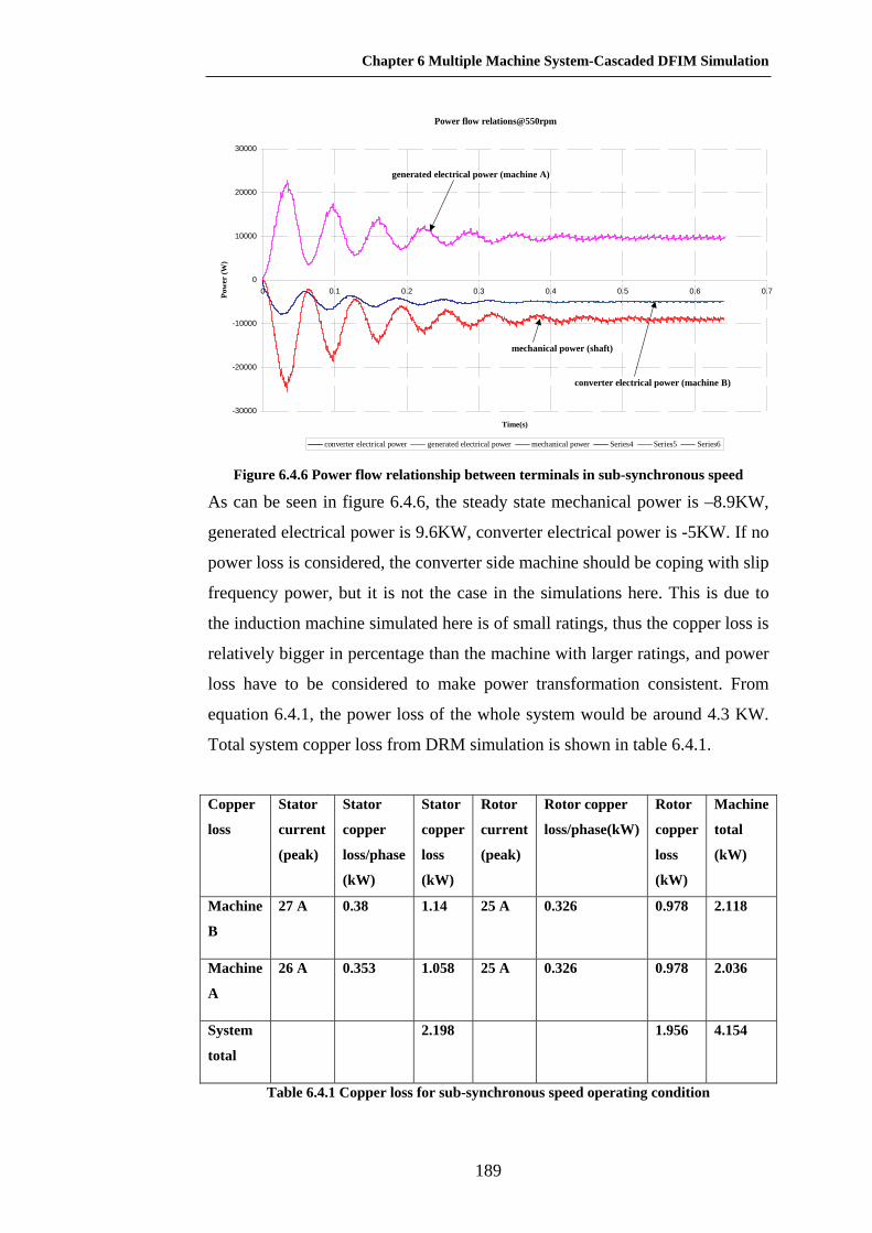
Chapter 6 Multiple Machine System-Cascaded DFIM Simulation
189
Power flow relations@550rpm
-30000
-20000
-10000
0
10000
20000
30000
0 0.1 0.2 0.3 0.4 0.5 0.6 0.7
Time(s)
Pow
er (W
)
converter electrical power generated electrical power mechanical power Series4 Series5 Series6
generated electrical power (machine A)
converter electrical power (machine B)
mechanical power (shaft)
Figure 6.4.6 Power flow relationship between terminals in sub-synchronous speed
As can be seen in figure 6.4.6, the steady state mechanical power is –8.9KW,
generated electrical power is 9.6KW, converter electrical power is -5KW. If no
power loss is considered, the converter side machine should be coping with slip
frequency power, but it is not the case in the simulations here. This is due to
the induction machine simulated here is of small ratings, thus the copper loss is
relatively bigger in percentage than the machine with larger ratings, and power
loss have to be considered to make power transformation consistent. From
equation 6.4.1, the power loss of the whole system would be around 4.3 KW.
Total system copper loss from DRM simulation is shown in table 6.4.1.
Copper
loss
Stator
current
(peak)
Stator
copper
loss/phase
(kW)
Stator
copper
loss
(kW)
Rotor
current
(peak)
Rotor copper
loss/phase(kW)
Rotor
copper
loss
(kW)
Machine
total
(kW)
Machine
B
27 A 0.38 1.14 25 A 0.326 0.978 2.118
Machine
A
26 A 0.353 1.058 25 A 0.326 0.978 2.036
System
total
2.198 1.956 4.154
Table 6.4.1 Copper loss for sub-synchronous speed operating condition

Chapter 6 Multiple Machine System-Cascaded DFIM Simulation
190
The power loss difference between 4.3 KW and the copper loss, which is 4.154
KW, would be the computation errors, caused probably by the inaccurate
calculation of the rms value of currents during the loss calculations as well as
harmonics losses.
6.4.2 Super-synchronous speed, shaft speed - 950rpm
For super-synchronous speed, the frequency relations between the stator flux
and rotor flux fields for the two induction machines are different from that of
sub-synchronous speed.
Figure 6.4.7 Frequency relations in super-synchronous speed – 950 rpm for CDFM
Figure 6.4.7 shows the frequency relations for super-synchronous speed. Flux
field rotating direction for the stator flux field for converter side machine B is
opposite to that of sub-synchronous speed. And such cause the machine B rotor
flux field rotating frequency changed with respect to shaft. With a different
mechanical speed of the shaft, and a corresponded rotor flux field frequency,
50 Hz stator current comes out of the stator terminals of the grid side induction
machine, thus, a constant frequency, variable speed cascaded doubly fed

Chapter 6 Multiple Machine System-Cascaded DFIM Simulation
191
induction machine system is fulfilled. Currents in stator and rotor in the
cascaded machine system could be shown from figure 6.4.8 to 6.4.10.
converter side stator (machine B) current@950rpm
-60
-40
-20
0
20
40
60
80
0 0.1 0.2 0.3 0.4 0.5 0.6 0.7
Time (s)
Mac
hine
B st
ator
cur
rent
(Am
ps)
Figure 6.4.8 Converter side (side 4) induction machine stator current waveform
Stator current frequency of machine B in figure 6.4.8 is 13.3 Hz, calculated
based on the running condition of the shaft speed. It is the frequency of the
applied voltage through converter to machine B’s stator,.
Rotor phase A current@950 rpm
-60
-40
-20
0
20
40
60
80
0 0.1 0.2 0.3 0.4 0.5 0.6 0.7
Time(s)
Rot
or p
hase
A c
urre
nt (A
mps
)
Figure 6.4.9 Rotor current waveform (side 2 & 3)
Rotor current frequency in super-synchronous speed 950 rpm in figure 6.4.9 is
18.33 Hz, as what is expected in figure 6.4.7.

Chapter 6 Multiple Machine System-Cascaded DFIM Simulation
192
grid side stator (machine A) current@950 rpm
-80
-60
-40
-20
0
20
40
60
80
0 0.1 0.2 0.3 0.4 0.5 0.6 0.7
Time(s)
Mac
hine
A st
ator
cur
rent
(Am
ps)
Figure 6.4.10 Grid side (side 1) induction machine generated current waveform
Figure 6.4.10 shows the generated stator current waveform for machine A, its
frequency is 50 Hz, the same with theoretical value.
Power flow relations in super-synchronous speed are shown in figure 6.4.11.
Figure 6.4.11 Power flow condition in super-synchronous speed
For super-synchronous speed running condition, power relations inside the
cascaded machine system follows the same power relations as shown in
equations 6.4.1. But, due to the super-synchronous speed the system is
operating, converter electrical power will flow out of the machine system
instead of flowing into, as shown by the arrow in figure 6.4.11. DRM
simulation for power flow condition in super-synchronous running state is
shown in figure 6.4.12.

Chapter 6 Multiple Machine System-Cascaded DFIM Simulation
193
Power flow relation @950 rpm
-120000
-100000
-80000
-60000
-40000
-20000
0
20000
40000
60000
80000
0 0.1 0.2 0.3 0.4 0.5 0.6 0.7
Time(s)
Pow
er (W
)
converter electrical power generated electrical power mechanical power Series4 Series5 Series6
generated electrical power (machine A) converter electrical power (machine B)
mechanical power (shaft)
Figure 6.4.12 Grid side induction machine stator current waveform (side 1)
As can be seen from figure 6.4.12, converter electrical power changed the sign
to positive, which means power is flowing out of side 4 to the grid. This is
what is expected in theory. The mechanical power is -33.7KW, generated
electrical power is 19.07 KW, and the converter electrical power is 6 KW.
From equations 6.4.1, power loss of the whole system would be around 8.63
KW. Total system copper loss from DRM simulations for super-synchronous
speed 950 rpm is shown in Table 6.4.2.
Stator
current
(peak)
Stator
copper
loss/phase
(kW)
Stator
copper
loss
(kW)
Rotor
current
(peak)
Rotor
copper
loss/phase
(kW)
Rotor
copper
loss
(kW)
Machine
total
(kW)
Machine
B
40 A 0.835 2.5 35.6 A 0.66 1.98 3.48
Machine
A
36 A 0.676 2.03 35.6 A 0.66 1.98 4.01
System
total
4.53 3.96 7.49
Table 6.4.2 Copper loss for super-synchronous speed operating condition
Power loss difference between 8.63 kW and 7.49 kW copper losses is the
computational errors.

Chapter 6 Multiple Machine System-Cascaded DFIM Simulation
194
6.4.3 Synchronous speed, shaft speed - 750 rpm
In synchronous speed, d.c. voltage is applied to the stator of converter side
machine, as shown in figure 6.4.13.
Figure 6.4.13 Frequency relations in synchronous speed – 750 rpm for CDFM
As can be seen from figure 6.4.13, stator flux field for machine B is stationary
due to the d.c. voltage applied to it. To maintain the same direction and
frequency of the stator flux field, rotor flux field rotating direction would be in
the opposite direction to the shaft rotating direction with respect to the shaft,
such that the total rotor flux field would be stationary to the frame. After
machine A’s rotor flux field rotating direction is changed by swapped phases,
50 Hz stator currents are generated from machine A, side 1, as shown in figure
6.4.13. Figure 6.4.14 to 6.4.16 show the current waveform of synchronous
speed running condition for CDFM.

Chapter 6 Multiple Machine System-Cascaded DFIM Simulation
195
converter stator phase A current (side 4) @750 rpm
-5
0
5
10
15
20
25
0 0.1 0.2 0.3 0.4 0.5 0.6 0.7
Time (s)
Mac
hine
B st
ator
cur
rent
(Am
ps)
(a)
Converter stator phase B current (side 4) @750 rpm
0
5
10
15
20
25
0 0.1 0.2 0.3 0.4 0.5 0.6 0.7
Time (s)
Mac
hine
B p
hase
B c
urre
nt
(b)

Chapter 6 Multiple Machine System-Cascaded DFIM Simulation
196
Converter stator phase C current (side 4) @750 rpm
-25
-20
-15
-10
-5
00 0.1 0.2 0.3 0.4 0.5 0.6 0.7
Time (s)
Mac
hine
B p
hae
C c
urre
nt (A
mps
)
(c)
Figure 6.4.14 Converter side (side 4) stator current waveform
Figure 6.4.14 shows the three-phase stator current of machine B. Phase B and
C are d.c. current practically, and phase A current is zero in steady state. This
is due to the 0 frequency sinusoidal waveform applied the stator terminals in
machine B.
Rotor current (side 2 and 3)
-20
-15
-10
-5
0
5
10
15
20
0 0.1 0.2 0.3 0.4 0.5 0.6 0.7
Time (s)
Rot
or c
urre
nt (A
mps
)
Figure 6.4.15 Cascaded machine rotor phase A current (side 2 and 3)
Rotor current frequency is 25 Hz, as what is expected in synchronous running
condition.

Chapter 6 Multiple Machine System-Cascaded DFIM Simulation
197
Generated stator current (side 1)
-20
-15
-10
-5
0
5
10
15
20
25
0 0.1 0.2 0.3 0.4 0.5 0.6 0.7
Time (s)
Mac
hine
A st
ator
cur
rent
(Am
ps)
Figure 6.4.16 Generated grid side stator current waveform (side 1)
Figure 6.4.16 shows the generated stator current waveform for machine A in
synchronous running condition, its frequency is 50 Hz, as what is expected.
In synchronous speed, converter power only handles the power to iron loss, as
have been stated in previous sections. Power flow condition can be seen in
figure 6.4.17.
Figure 6.4.17 Power flow condition in synchronous speed for CDFM system
Converter power is supposed to be flowing into the CDFM system to
compensate for the system losses. Power relations as shown in equations 6.4.1
should be satisfied. DRM simulation result for power flow is shown in figure
6.4.18.

Chapter 6 Multiple Machine System-Cascaded DFIM Simulation
198
Power flow relations @750 rpm
-8000
-6000
-4000
-2000
0
2000
4000
6000
0 0.1 0.2 0.3 0.4 0.5 0.6 0.7
Time (s)
Pow
er (W
)
converter electrical power generated electrical power mechanical power
generated electrical power (machine A)
mechanical power (shaft)
converter side electrical power (machine B)
Figure 6.4.18 Power flow relationship between terminals in synchronous speed
As can be seen in figure 6.4.18, the mechanical power in steady state is 4.09
KW, generated electrical power is 3.12 kW, and converter electrical power is
0.414kW. From the calculation in equations 6.4.1, the total power loss in the
system would be around 1.384 kW. Total system copper loss from DRM
simulations is shown in Table 6.4.2.
Stator
current
(d.c)
Stator
copper
loss/phase
A (kW)
Stator
copper
loss
(kW)
Rotor
current
(peak)
Rotor
copper
loss/phase
(kW)
Rotor
copper
loss
(kW)
Machine
total
(kW)
Machine
B
14 A 0.204 0.408 14 A 0.102 0.306 0.714
Machine
A
15 A 0.117 0.352 14 A 0.102 0.306 0.658
System
total
0.76 0.612 1.372
Table 6.4.3 Copper loss for synchronous speed operation
The power difference between 1.372 kW for copper loss and 1.384 kW for
total system loss is due to computational errors.
With the help of DRM simulation, the frequency relationship and power flow
conditions in three operations state for cascaded doubly fed induction machine
have been simulated and analysed. One thing needs to be pointed out is that;
Chapter 6 Multiple Machine System-Cascaded DFIM Simulation
199
obvious harmonics distortion can be spotted in power flow conditions figures
for all of the three running conditions. This is due to the slot harmonics in the
two machines, and might cause control problem for the controls in cascaded
machine systems.
6.5 Conclusion
This chapter extends the DRM modelling method further to the modelling and
simulation of the multiple-machine, system-cascaded, doubly-fed, induction
machine system, which involves two cascaded induction machines to replace
the slip ring in doubly fed induction generators. Simulation results are
investigated considering sub-synchronous speed, super-synchronous speed and
synchronous speed respectively. Power flow conditions and current frequencies
are investigated as well.
There are slotting harmonic effects which show through as distortion in the
current waveforms and are clearer in the power waveforms. These effects in
this case are not particularly strong but could fall into the current bandwidth of
the current controllers of a practical system and may well cause voltage
distortion. However, the simulation here is for small power machines which are
skewed thus substantially suppressing the slotting effects. Skewing is much
less common in high power machines and practical designs may therefore see
considerably greater slotting problems if they are not designed appropriately.
The DRM approach obviously has the capability to assist fully in exploring and
controlling these design problems.

Chapter 7 Reluctance Mesh Topology Investigation in the DRM Modelling Method
200
CHAPTER 7 RELUCTANCE MESH TOPOLOGY
INVESTIGATION IN THE DYNAMIC RELUCTANCE
MESH MODELLING METHOD
7.1 Introduction
Dynamic Reluctance Mesh modelling is an effective way to model and
simulate electrical machines and multiple machine systems, as have been
studied and validated in chapter 4, 5 and 6. The accuracy of the simulation
results from DRM model depends on many aspects, including the topology of
the reluctance mesh, the numerical parameter settings as well as the solving
accuracy of the solver. Among them, the topology of the reluctance mesh is a
key factor.
However, the creation of the topology of reluctance mesh is determined by
experience, based on the prior known knowledge of the flux distribution inside
the electrical machines, both the iron part and the air gap part. Different
topology of reluctance mesh will give different machine simulation behaviour;
and the different modelling of the air gap region, which involves leakage flux
modelling, gives the most differences.
This chapter will concentrate on the influence of reluctance mesh topology on
machine simulation results. The influence of the modelling of slot leakage flux
in induction machines; the discretisation of stator tooth tips in exciter and the
discretisation of salient pole iron part will be investigated and discussed
separately. The objective of the work in this chapter is to determine what is
important in reluctance mesh creation based upon the prior knowledge of flux
distribution in the machine.

Chapter 7 Reluctance Mesh Topology Investigation in the DRM Modelling Method
201
7.2 Induction Machine Reluctance Mesh Investigation
As described in section 3.5, there are leakage fluxes flowing linking windings
in the stator and rotor slots, thus, an additional reluctance representing leakage
flux between stator and rotor teeth needs to be added, as shown in figure 7.2.1.
Topologies using 1, 2 and 3 mmfs are modelled in the tooth part of the
induction machine, with corresponds to 1 reluctance representing leakage flux,
2 reluctances and 3 reluctances.
Figure 7.2.1 Induction machine reluctance mesh topology
considering leakage flux across slots
In each case, if the magnetic steel of the teeth is perfect and has infinite
permeability, the leakage flux values obtained will be the same. However, with
finite permeability and particularly with high levels of saturation the three
models will not yield the same leakage flux.
Figure 7.2.2 shows the DRM simulation results for a non-skewed rotor
induction machine, with 1mmf, 2mmfs, and 3mmfs in stator and rotor
reluctance mesh. Reluctances represent leakage fluxes in between stator and
rotor slots and are calculated by leakage reluctance calculation method given in
section 3.5.

Chapter 7 Reluctance Mesh Topology Investigation in the DRM Modelling Method
202
Induction machine DOL start, speed
-200
0
200
400
600
800
1000
1200
1400
1600
1800
0 0.01 0.02 0.03 0.04 0.05 0.06 0.07 0.08 0.09 0.1
Time (s)
Spee
d (r
pm)
1 MMF
2MMF
3MMF
FEM
Figure 7.2.2 DRM simulation result of induction machine speed rising curve, with 1mmf,
2mmfs and 3mmfs in reluctance mesh
As can see from figure 7.2.2, the simulation results from the reluctance mesh
with 2mmfs and 3mmfs give a better agreement to FEM result compared to the
result given by 1mmf. The reason is that the slope of the acceleration curve of
the induction machine depends on the rate of rise of flux and current inside the
machine, which is influenced primarily by leakage flux. By modelling the
leakage flux reluctance between stator and rotor slots for the 2mmfs and
3mmfs modelling, the leakage effects in the machine is accounted for more
effectively as it is a distributed phenomena. Initially all three curves agree
because there is limited winding current and the acceleration is very low. As
the winding currents build up to several times the rated value saturation of the
leakage flux paths in the teeth become significant and the acceleration curves
diverge. Thus a better agreement of the acceleration curve compared to the
FEM result occurred with the 3 mmf model which allows for this saturation
effect more effectively.
Therefore, in DRM modelling, the additional reluctances representing
distributed leakage flux in the machine should be created to account for
leakage flux, particularly when the machine transient behaviour, which is
considerably affected by leakage effects, is the research interest. Quite
satisfactory results can be obtained by using 2 mmf sources per tooth though 3

Chapter 7 Reluctance Mesh Topology Investigation in the DRM Modelling Method
203
would be better in critical cases. There appears to be no need to use more than
3 mmf sources per tooth in normal machines.
7.3 Exciter Reluctance Mesh Investigation
Exciters have a slightly different geometry in the respect of the relative width
of the stator and rotor tooth tips in comparison to induction machines: the tooth
tip widths of the stator and rotor in the induction machine are in a similar range
while for an exciter, the stator tooth tip is much wider than that of the rotor.
This is due to the machine type, i.e. salient pole, and a small number of
armature slots for cost reasons in exciter. For the exciter, high frequency
currents are generated to feed to the rotating rectifier and then to the generator
field winding. The number of poles in the exciter is commonly much more than
that of the induction machine. Also, d.c. is applied to the exciter stator, and the
number of stator teeth is designed to be equal to the number of poles, avoiding
a complicated a.c. winding to reduce manufacturing cost. Therefore, the
reluctance mesh discretisation of the stator tooth tip in exciter could be the
same as that of induction machine from the geometry perception, but also
could be different considering the wider stator tooth tip width with respect to
the rotor tooth tip width.
In this section, three different discretisations of the exciter stator tooth tip will
be used in DRM simulations, shown in figure 7.3.1 to figure 7.3.3, and then
their resultant machine behaviour will be examined and compared.

Chapter 7 Reluctance Mesh Topology Investigation in the DRM Modelling Method
204
Figure 7.3.1 Reluctance mesh of the exciter, type 1: one reluctance on stator tooth tip
Figure 7.3.2 Reluctance mesh of the exciter, type 2: three reluctances on stator tooth tip

Chapter 7 Reluctance Mesh Topology Investigation in the DRM Modelling Method
205
Figure 7.3.3 Reluctance mesh of the exciter, type 3: four reluctances on stator tooth tip
When comparing figure 7.3.1, figure 7.3.2 and figure 7.3.3, differences of these
reluctance meshes are the number of elements in the stator tooth tip area. It can
be seen that exciter stator teeth is divided into three elements in mesh type 2
and into four in type 3 respectively, but only divided to one in mesh type 1.
For mesh type 2, the width of each virtual tooth in the stator is of the similar
width with that of rotor. The reason why reluctance mesh type 2 and 3 are
utilized is because the flux distribution is assumed to be normal to the tooth
surface (constant potential surface) in mesh type one, although practically this
may not be the case due to saturation reducing the relative permeability. Some
of the flux distribution in the tip region of the tooth will be distorted due to the
different geometry of tip area and tooth region. By dividing the tooth surface
into more than one reluctance element, this flux distortion can be accounted for.
In each case however, a finite element model of the air gap and teeth has been
used to work out the air gap reluctances which are to be used. Air gap
reluctance curves for these three types of stator tip discretisation are shown in
figure 7.3.4. It can be seen that the air gap curves have different width and
magnitude due to the different discretisations.

Chapter 7 Reluctance Mesh Topology Investigation in the DRM Modelling Method
206
Air gap curves for exciter
-0.002
0
0.002
0.004
0.006
0.008
0.01
0.012
0.014
-0.5 -0.4 -0.3 -0.2 -0.1 0 0.1 0.2 0.3 0.4 0.5
Offset (RAD)
Eff
ectiv
e w
idth
(m)
2&3r 1&4 CENTRAL SIDE single
1 stator tip reluctance
3 stator tip reluctance (central and side curves)
4 stator tip reluctance(central and side curves)
Figure 7.3.4 Air gap reluctance curves for the three discretisations
for exciter stator tooth tip
The relatively wide center part of the air gap reluctance curve for 1 stator tip
reluctance is explained by the much wider stator tooth tip width compared to
the rotor tooth tip width. Thus a constant air gap reluctance width is expected
while rotor tooth is within the stator tooth region.
Comparison of DRM simulation results for these different types of reluctance
mesh in a simulated open circuit case are shown in figure 7.3.5 to 7.3.7. It can
be seen that the current and voltage ripple are bigger for reluctance mesh type 2
and 3 compared to mesh type 1.

Chapter 7 Reluctance Mesh Topology Investigation in the DRM Modelling Method
207
Exciter stator current comparison
0.5
0.52
0.54
0.56
0.58
0.6
0.62
0.64
0.66
0.5 0.502 0.504 0.506 0.508 0.51
Time (s)
Stat
or c
urre
nt (A
mps
)
stator 3 tip elements stator 1 tip element stator 4 tip elements
stator 3 tip elements stator 4 tip elements
stator 1 tip elements
Figure 7.3.5 Exciter stator current comparisons for different reluctance meshes, mesh
type 1,2&3
Stator current ripple, as shown in figure 7.3.5, has the slot harmonic ripple
caused by the slot opening on the rotating rotor. Its frequency is the slot
passing frequency, which is 10504225 =× [28]. It can be seen that mesh 2 and
mesh 3 give a bigger ripple due to the different way of modelling the tip
elements that touch the air gap. More elements on tooth tip area can account
for the flux non-uniform distribution in the tooth tip area but cause an effect of
ripple in stator current. This is due to the division of the stator tooth producing
virtual teeth on the stator. However, if there was not appreciable saturation of
the stator tooth tip elements there would be no appreciable difference between
the models.
Figure 7.3.6 shows the exciter rotor current for the three different kinds of
reluctance meshes. It can be seen that mesh type 1 and mesh type 3 give a
similar average exciter rotor current waveform, although result for mesh 3 has
more harmonics, which is due to the additional discretisation on stator teeth.
There are bigger exciter rotor current harmonics in the result of mesh type 2,
compared to mesh type 1 and 2. It looks like mesh 2 gives a substantial
cogging effect, the same as for induction machines, when the number of stator
teeth equals the number of rotor teeth. In mesh type 2, the number of virtual
teeth of exciter stator is 42, while the number of rotor teeth of this exciter is

Chapter 7 Reluctance Mesh Topology Investigation in the DRM Modelling Method
208
also 42, the same number of teeth for exciter stator virtual teeth. According to
Alger [25], cogging effect due to stator and rotor having same number of teeth
happens.
Exciter rotor phase current
-0.015
-0.01
-0.005
0
0.005
0.01
0.015
0.5 0.502 0.504 0.506 0.508 0.51
Time(s)
Rot
or c
urre
nt(A
mps
)
stator 3 tip elements stator 1 tip element stator 4 tip elements
stator 3 tip elements
stator 4 tip elements
stator 1 tip elements
Figure 7.3.6 Exciter rotor current comparison for different reluctance meshes, mesh type
1,2&3 Exciter open circuit rotor voltage
-30
-20
-10
0
10
20
30
0.5 0.502 0.504 0.506 0.508 0.51
Time(s)
Rot
or v
olta
ge(V
olt)
stator 3 tip elements stator 1 tip element stator 4 tip elements
stator 3 tips elements
stator 4 tip elements
stator 1 tip element
Figure 7.3.7 Exciter rotor terminal open circuit voltage comparison for mesh type 1,2&3
This cogging effect could also be seen from figure 7.3.7, the exciter open
circuit rotor terminal voltage waveforms. It can be seen that compared with
mesh type 1 and 3, result comes out from mesh type 2 has obvious cogging.

Chapter 7 Reluctance Mesh Topology Investigation in the DRM Modelling Method
209
With different discretisation approaches for the stator tooth tip in the exciter,
different currents and voltage waveforms for the stator and rotor could be
achieved. Each of them reflects real machine behaviour in some aspect, and
tooth harmonics effects could be simulated. However, the only real difference
between the models is the stator tooth tip reluctance elements. If the tooth tip
elements of the models 2 and 3 become zero then these models reduce to model
1. This would suggest that there is a fair degree of saturation in the tooth tips of
the exciter under normal operating conditions.
The conclusion here is that not only is it necessary to apply the concept of
virtual teeth with salient pole forms of machine but it is also necessary to
model the air gap reluctances and tooth tip reluctances effectively. This is
particularly true for machines with saturated salient pole tips under normal or
faulty operating conditions.
7.4 Salient Pole Synchronous Generator Reluctance Mesh
Investigation
Considering the reluctance mesh for salient pole synchronous generator, two
types of reluctance mesh will be investigated in this section: one with 6 virtual
teeth on the central pole, while the other one with doubled the virtual teeth in
the central part of the salient pole. The geometry of the salient pole examined
in this section has a stepped airgap in the middle of the salient pole,
specifications of this machine is detailed in Appendix 6. The two reluctance
meshes to be investigated are shown in figure 7.4.1 & 7.4.2, referenced as
DRM case 1 and DRM case 2.
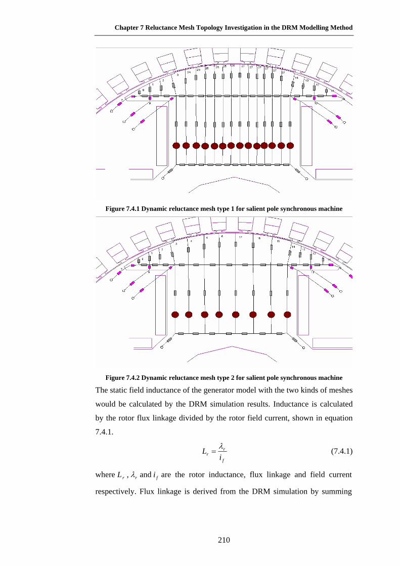
Chapter 7 Reluctance Mesh Topology Investigation in the DRM Modelling Method
210
Figure 7.4.1 Dynamic reluctance mesh type 1 for salient pole synchronous machine
Figure 7.4.2 Dynamic reluctance mesh type 2 for salient pole synchronous machine
The static field inductance of the generator model with the two kinds of meshes
would be calculated by the DRM simulation results. Inductance is calculated
by the rotor flux linkage divided by the rotor field current, shown in equation
7.4.1.
f
rr i
L λ= (7.4.1)
where rL , rλ and fi are the rotor inductance, flux linkage and field current
respectively. Flux linkage is derived from the DRM simulation by summing
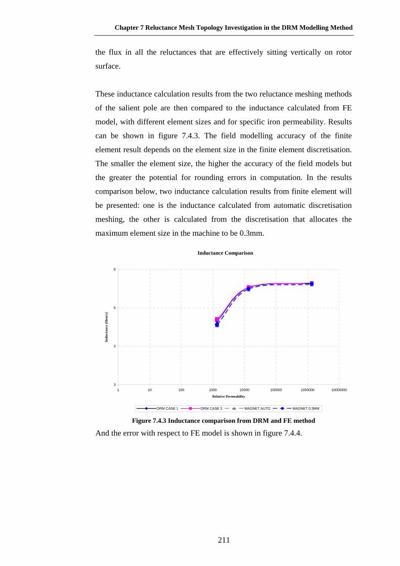
Chapter 7 Reluctance Mesh Topology Investigation in the DRM Modelling Method
211
the flux in all the reluctances that are effectively sitting vertically on rotor
surface.
These inductance calculation results from the two reluctance meshing methods
of the salient pole are then compared to the inductance calculated from FE
model, with different element sizes and for specific iron permeability. Results
can be shown in figure 7.4.3. The field modelling accuracy of the finite
element result depends on the element size in the finite element discretisation.
The smaller the element size, the higher the accuracy of the field models but
the greater the potential for rounding errors in computation. In the results
comparison below, two inductance calculation results from finite element will
be presented: one is the inductance calculated from automatic discretisation
meshing, the other is calculated from the discretisation that allocates the
maximum element size in the machine to be 0.3mm.
Inductance Comparison
3
4
5
6
1 10 100 1000 10000 100000 1000000 10000000
Relative Permeability
Indu
ctan
ce (H
enry
)
DRM CASE 1 DRM CASE 2 MAGNET AUTO MAGNET 0.3MM
Figure 7.4.3 Inductance comparison from DRM and FE method
And the error with respect to FE model is shown in figure 7.4.4.

Chapter 7 Reluctance Mesh Topology Investigation in the DRM Modelling Method
212
Inductance Error
0
0.5
1
1.5
2
2.5
3
3.5
1 10 100 1000 10000 100000 1000000 10000000
Relative Permeability
Err
or%
DRM CASE 1 TO AUTO DRM CASE 2 TO AUTO
DRM CASE 1 TO 0.3 MAGNET DRM CASE 2 TO 0.3 MAGNET
DRM case 1 to FE
DRM case 2 to FE
Figure 7.4.4 Inductance comparison error for DRM with respect to FE It can be seen that DRM case 1 produces less error compared to finite element
results, than DRM case 2, which means that the more number of iron elements
discretised, the more accurate the result would be, even for the central salient
pole part which conducts main flux in machine’s magnetic circuit. All the
errors decrease with the increase of the iron permeability. Permeability is
involved in the result sheet is because the air gap overlap curve that has been
used in the salient pole synchronous machine DRM simulation is derived from
a simplified FE model with a very big permeability ( 135000=rµ ), while in
the DRM simulations in this section, the iron permeability used in DRM
simulation is not that big, and this will result in a discrepancy between the
DRM and FE simulation results, shown in figure 7.4.4. The larger the iron
permeability used in DRM simulations, the closer the simulation result will be
to the FE result.
It can also be seen that the smaller the element size in the FE model, the
smaller the errors, which proves the rule that the smaller elements size makes a
more accurate field model.

Chapter 7 Reluctance Mesh Topology Investigation in the DRM Modelling Method
213
In this section, by comparing different ways of discretising iron elements in a
salient pole, the effect of iron discretisation has been investigated. It is shown
from the result that the discretisation in unsaturated iron doesn’t influence the
simulation result a lot, from the inductance point of view.
7.5 Influence of the Reluctance Mesh in a Single Machine to
Multiple Machine System
In previous sections, different reluctance mesh topologies for induction
machines, exciters and salient pole synchronous machines have been
investigated individually. In this section, the influence of the reluctance mesh
for one machine in a multiple machine system will be examined.
This section will look at the mesh discretisation influence in DRM simulations
for the brushless generating system that has been simulated and investigated in
chapter 5. Different exciter stator reluctance meshes are applied, and the whole
system open circuit curves will be derived and comparison will be made to
experimental results. Different reluctance mesh for exciter is applied here
instead of for salient pole rotor is because the exciter is non-skewed, thus a
saturation effect is prominent and could be spotted easily.
By applying the exciter stator reluctance model type 1 and 2, the open circuit
curve of the whole system is shown below in Figure 7.5.1.

Chapter 7 Reluctance Mesh Topology Investigation in the DRM Modelling Method
214
Open Circuit Comparison for complete brushless generating system
0
50
100
150
200
250
300
350
400
450
0 2 4 6 8 10 12
Exciter stator voltage (Volts)
Gen
erat
or st
ator
vol
tage
(Vol
ts)
Modified experimental result exciter stator 1 tip reluctance exciter stator 3 tip elements
stator 1 tip element
stator 3 tip elements
modified experimental result
Figure 7.5.1 Open circuit test simulation result comparison for generating system, with
different reluctance mesh of exciter
Clearly the greater discretisation of the exciter stator poles not only influences
the harmonic content of the rotor current waveform as seen in the previous
section, but also alters the shape of the open circuit curve for the brushless
generator. It is clear that the exciter must have saturated pole tips and suffer

Chapter 7 Reluctance Mesh Topology Investigation in the DRM Modelling Method
215
from armature reaction since increasing the number of virtual stator teeth
increases the agreement between experimental and simulated results. Armature
reaction increases with exciter load current and reduces the net flux in the
exciter producing a lower field current in the main generator. The results show
better agreement between the models at low generator output voltage and thus
low load and low armature reaction conditions in the exciter. As generator
output voltage increases the open circuit curves of the different models diverge
and the lower discretisation models which cannot evaluate armature reaction in
the exciter effectively, become increasingly in error.
It is quite difficult to obtain experimentally the rotor current waveforms of the
exciter when it is operating as part of a brushless generator set simply because
the signals are on the rotating rotor. However, the overall system performance
yields sufficient information when the additional component models have
already been verified as accurate. It appears that to obtain sufficient accuracy,
the number of virtual teeth on each stator pole has to be similar to, or slightly
greater than the actual number of teeth on the rotor since 3 virtual teeth gives
very good results for a rotor with 3 teeth per pole in this case.
7.6 Conclusion
The accuracy of DRM modelling technique depends partly on the topology of
the reluctance mesh. The topology of the reluctance mesh is decided by the
prior knowledge of the flux distribution in the machine. This chapter
investigated the influence of the different reluctance mesh forms on the DRM
simulation results, taking the exciter machine, salient pole generator and the
whole generating system as examples. The objective was to examine what is
important in terms of this prior knowledge.
The research has confirmed the importance of modelling in detail the leakage
reluctances in a machine where high winding currents under transient
conditions cause saturation of leakage flux paths. There is also a need to use
virtual teeth with salient pole machines if saturation of the pole is to be

Chapter 7 Reluctance Mesh Topology Investigation in the DRM Modelling Method
216
considered as is almost inevitable due to armature reaction. This has been
clearly demonstrated with the open circuit curves for the brushless generator
when different virtual teeth numbers have been examined for the exciter. The
results show that a similar number of virtual teeth are required to the actual
number of teeth carrying the armature winding.
A further conclusion is that when using the finite element models to evaluate
the air gap reluctance values it is best to use permeance values for the iron
parts of the machine which approximate to the values likely to be found under
normal operating conditions associated with the main flux path.

Chapter 8 Conclusions and Future Work
217
CHAPTER 8 CONCLUSION AND FUTURE WORK
8.1 Introduction
This chapter summarizes the main conclusions drawn from the thesis and
discusses relevant future work of this research area.
8.2 Conclusion
This thesis developed and validated a computationally efficient, detailed,
modelling method for electrical machine simulations derived from field
behaviour. It is suitable for machines with both uniform and non uniform air
gaps such as induction motors and salient pole synchronous generators
respectively. It is particularly suitable for modelling multiple machine systems
which may include nonlinear power electronic components and control
schemes. The method is based on and extends greatly, simple, traditional, finite
difference, lumped reluctance, machine models. Comparison of results between
DRM simulations and those obtained using finite elements as well as those
obtained experimentally have shown that this method gives excellent
agreement within engineering accuracies. Furthermore, this method can also be
applied to other related systems with complicated control and power electronic
schemes in place.
The modelling approach developed in this thesis sits between system modelling
using SIMULINK and idealised dq machine models and the finite element
modelling of individual machines. Commercial finite-element models are just
beginning to include control systems but they still do not include multiple
machine systems and control. In its current form the DRM program does not
have the flexibility of SIMULINK but it includes saturation of main and

Chapter 8 Conclusions and Future Work
218
leakage flux paths, slotting and space harmonic effects in detail in the machine
models which dq analysis can not do. While the DRM machine models
evaluate effectively all of the major factors which make machines non ideal,
they are not as comprehensive as a full finite element model developed
specifically for a particular machine. However, being computationally efficient
they take far less time to solve than FEM models offering iterative design
procedures not only for the machine but also for the system.
A summery of the research work and detailed conclusions is presented in each
of the relevant chapters. However, the main conclusions are summarized as
follows:
In the modelling of electrical machines, a more accurate method of modelling
the air gap reluctance in the DRM method, called air gap overlap curves, was
proposed based upon the simulation results from FE calculations. This air gap
overlap curve method extracts the useful information about the flux distribution
between the stator and rotor in the machines which takes fringing effects into
account and thus a more accurate model of the air gap flux connection is
achieved. This method can be used in induction machines but it is particularly
useful for salient pole synchronous machine which have non-uniform air gap
geometry where it is difficult for the original air gap reluctance creation rules
of the DRM to be applied effectively. This thesis detailed the method of
deriving the air gap overlap curve for the salient pole synchronous generator in
chapter 4, and results from open circuit test and short circuit test as well as the
air gap flux density distribution have shown that they agree well with both the
FE result and experiments. However, this air gap overlap curve derived from
FE only works accurately for a moderately nonlinear iron; for a heavily
saturated iron, flux distribution as well as the overlap curves between the stator
and rotor will be slightly different.

Chapter 8 Conclusions and Future Work
219
Detailed DRM models for electrical machines, such as slot leakage modelling
in induction machine and inter pole flux modelling and damper bar modelling
in salient pole synchronous machines, were also addressed in the thesis. The
discretisation method of the solid rotor pole is also described, because it is
different from the reluctance mesh creation for induction machine previously
applied. Comparison of the DRM results to FE and experiments have shown
that when these measures are included, the DRM can supply simulation results
with a very good accuracy from the engineering perspective.
A key part of any finite difference or FE program is the non linear equation
solver. The Newton-Raphson solver originally used for the DRM software was
further improved to overcome the nonconverge problems when solving system
with great nonlinearity. A globally convergent NR solver was proposed
introducing line searching schemes to identify a proper Newton step. This
improvement increased the stability of the solving process thus enabling more
complicated system simulations which have significant nonlinearities and
control schemes will be tackled more easily. This expanded the field of
application of the DRM method.
This thesis also applied the DRM modelling technique to the simulation and
investigations of multiple machine systems, namely, the small brushless
generating system and the cascaded doubly fed induction generators used in the
wind generation industry. This is a significant advance on conventional
methods of simulating machine systems. Normally, system models are
analysed through traditional winding coil models. These machine models are
very limited and neglect many saturation, harmonic and slotting effects
inherent in a practical system. With the DRM machine modelling technique,
the complete system incorporating multiple machines and power electronic
components as well as control schemes can be simulated with the entire
practical machine features modelled. All this is achieved within a reasonable

Chapter 8 Conclusions and Future Work
220
computation time. This is a task which commercial FE could not cope with
nowadays.
To complete the research of the DRM modelling technique, the influence of
different reluctance mesh topologies on the machine behaviour was
investigated in chapter 7. Results comparison for different reluctance mesh
forms of calculated and experimental results show that more refined reluctance
mesh models may be needed where the iron is heavily saturated by main or
leakage fluxes. That is in deep stator slots where leakage fluxes contribute to
tooth saturation it is not sufficient to model the slot leakage in one reluctance
linking the tooth tips. Dividing the slots and teeth into two or three sections
along the length of the teeth introduces additional slot leakage flux paths across
the slots which share out this leakage flux and reduce excessive tooth
saturation. Two sections are adequate in most cases but three sections give very
good results. Additionally, it was shown that salient poles should be treated as a
number of parallel virtual teeth and that even in very heavily saturated
machines the number of virtual teeth should be similar, but not exactly equal to,
the number of teeth on the armature.
The findings above have fulfilled the original aims of the research program and
have widened the knowledge of multiple machine simulation techniques, and
also expanded the application field of the dynamic reluctance modelling
technique.
8.3 Suggestions for Future Work
There are a number of suggestions for future work which can extend the
understanding and application of the dynamic reluctance modelling method
and increase the DRM modelling accuracy. These are:

Chapter 8 Conclusions and Future Work
221
1. Air gap reluctance models in the machines can be improved to
accommodate heavily saturated iron. This could be implemented by
applying different air gap overlap curves depending on the saturation
degree, e.g. the flux density value in the stator or rotor teeth. Thus, different
flux distributions which depend upon the saturation of the iron can be
accounted for. This is particularly useful in the simulations where
saturation phenomena are important to the electrical machine’s behaviour.
2. More realistic models and complex control schemes for the AVR controller
can be applied to the simulation model of small brushless generating
systems, other than the simplest PID controller currently simulated in the
thesis. Their performance could be evaluated by the modified DRM
simulation tool in the thesis.
3. This modified DRM machine simulation tool might be applied to other
machines or machine system simulation fields, where various control
schemes and machine designs need to be evaluated but with a reasonable
simulation time. Such a case might be a full, doubly fed wind generator
system.

Appendix
222
APPENDIX 1 SALIENT POLE SYNCHRONOUS
GENERATING SYSTEM SPECIFICATIONS
1.1 Main generator technical details

Appendix
223

Appendix
224
1.2 Main generator rotor lamination drawings
Figure A1.2.1 Rotor lamination drawings

Appendix
225
1.3 Main generator stator and rotor details
Figure A1.3.1 Stator details

Appendix
226
Figure A1.3.2 Rotor details

Appendix
227
1.4 Exciter machine details
Figure A1.4.1 Exciter stator details
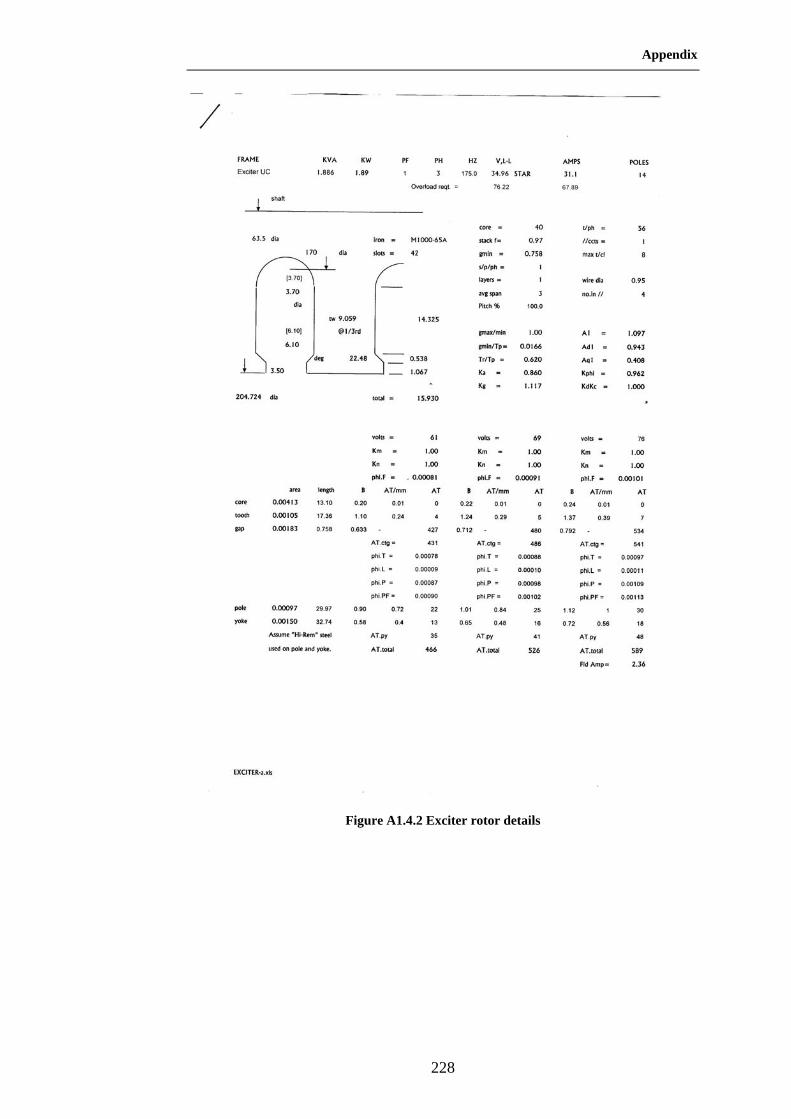
Appendix
228
Figure A1.4.2 Exciter rotor details

Appendix
229
APPENDIX 2 INDUCTION MACHINE SPECIFICATIONS Nameplate data: Manufacture Brook CromptonPhases 3Connection DeltaPoles 4Power 15 kwVolts 415 vFrequency 50 HzCurrent 27.08 ASpeed 1454 rpmTorque 99.5 NmEfficiency 0.891 Construction details Stator Figure 2.1Rotor Figure 2.2Inertia 086713 Kgm2Core Length 14.605 cmAir gap length 0.05842 cmStator slots 48Rotor slots 36 Stator winding details Conductors per slot 22Layers per slot 2Configuration three tier concentricCoil pitch 9 slots
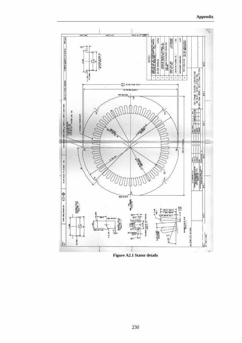
Appendix
230
Figure A2.1 Stator details

Appendix
231
Figure A2.2 Rotor details

Appendix
232
APPENDIX 3 RELUCTANCE CALCULATION METHOD
FOR SALIENT POLE ROTOR
This appendix will introduce how the iron reluctances in salient rotor pole are
calculated. Figure A3.1 shows the reluctance map for a salient rotor pole.
Reluctances in the left side of the rotor.
Figure A3.1 Salient pole reluctance mesh calculation graph
The left side of the salient rotor reluctance mesh in figure A3.1shows the
discretisation of the tangential flux inside the salient pole, and the right part
shows the discretisation of the radial flux inside the salient pole. Because the
symmetry of the pole, only half of the reluctance mesh for tangential flux and
radial flux is sufficient.
The area of each the reluctance in figure A3.1 is shown by the shadowed area
around the reluctance. Given the geometry of the salient pole, these reluctance
width, length and depth can be calculated as shown by figure A3.1.

Appendix
233
APPENDIX 4 FULL WAVE BRIDGE RECTIFIER
In Industrial applications, where three-phase a.c. voltages are available, it is
preferable to use three-phase rectifier circuits, compared to single-phase
rectifiers, because of their low ripple content in the waveform and a higher
power-handling capability. The three-phase, six-pulse, full-bridge diode
rectifier shown in figure A4.1 is a commonly used circuit arrangement.
Figure A4.1 Six diodes full wave three-phase bridge rectifier
The voltage waveforms for the circuit shown in figure A4.1 are shown in figure
A4.2, where the solid lines are the voltage across the resistance.
Figure A4.2 Voltage across resistance load in a full waveform bridge rectifier
In figure A4.2, pnv is the voltage of point P with respect to the a.c. voltage
neutral point n, and nnv is point N’s voltage, which is the negative d.c. terminal
voltage, with respect to neutral point. D.c. voltage across the resistance load
would be: ( N is the neutral voltage, ie zero and P is the positive terminal of the
resistive load or rectifier positive output. N is alos the negative voltage output
from the rectifier ie two separate things, hence Vnn is the voltage between

Appendix
234
negative and neutral. Vd is the effective output voltage across the resistive load
which moves up and down with respect to the neutral voltage)
nnpnd vvv −= (A4.1)
as shown in figure A4.3.
Figure A4.3 D.c voltage waveform of three phase full wave voltage rectifiers
By integrating dv , which has ripple in its waveform; we could derive the
average d.c. voltage dov :
( ) LLLLLLdo VVtdtVv 35.123cos23/
1 6/
6/=== ∫− π
ωωπ
π
π (A4.2)
and by using the definition of rms current in the phase current waveform,
which is a sinusoidal waveform, the rms value of line current si in this idealized
case is :
dds III 816.032
== (A4.3)
and fundamental-frequency component 1si of ac line current has an rms value:
dds III 78.0611 ==
π (A4.4)
where dI is the current flowing through the resistive load.

Appendix
235
In this kind of full wave bridge rectifier, each diode conducts for 120’, as
shown in figure A4.4.
Figure A4.4 Time sequence of conducting of each diode in full wave bridge rectifier
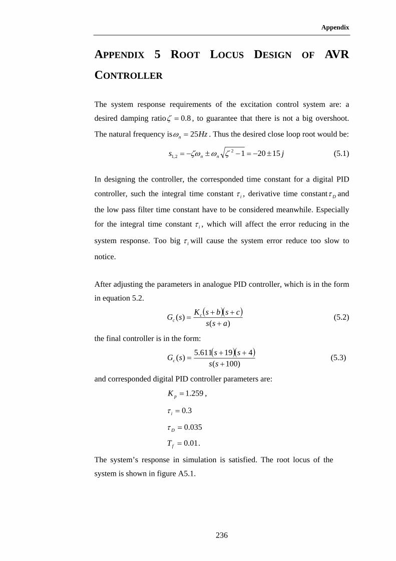
Appendix
236
APPENDIX 5 ROOT LOCUS DESIGN OF AVR
CONTROLLER
The system response requirements of the excitation control system are: a
desired damping ratio 8.0=ζ , to guarantee that there is not a big overshoot.
The natural frequency is Hzn 25=ω . Thus the desired close loop root would be:
js nn 1520122,1 ±−=−±−= ζωζω (5.1)
In designing the controller, the corresponded time constant for a digital PID
controller, such the integral time constant iτ , derivative time constant Dτ and
the low pass filter time constant have to be considered meanwhile. Especially
for the integral time constant iτ , which will affect the error reducing in the
system response. Too big iτ will cause the system error reduce too slow to
notice.
After adjusting the parameters in analogue PID controller, which is in the form
in equation 5.2.
( )( ))(
)(ass
csbsKsG cc +
++= (5.2)
the final controller is in the form:
( )( ))100(
419611.5)(+
++=
sssssGc (5.3)
and corresponded digital PID controller parameters are:
259.1=pK ,
3.0=iτ
035.0=Dτ
01.0=fT .
The system’s response in simulation is satisfied. The root locus of the
system is shown in figure A5.1.

Appendix
237
Root Locus
Real Axis
Imag
inar
y Ax
is
-100 -90 -80 -70 -60 -50 -40 -30 -20 -10 0-50
-40
-30
-20
-10
0
10
20
30
40
500.160.340.50.640.760.86
0.94
0.985
0.160.340.50.640.760.86
0.94
0.985
20406080
System: untitled1Gain: 1.01
Pole: -20 + 15iDamping: 0.8
Overshoot (%): 1.52Frequency (rad/sec): 25
Figure A5.1 Root locus of AVR controller
It can be seen that the root locus of the system pass the design point, thus the
design requirements are satisfied.
Once the transfer function of the controller in frequency domain is derived, in
order to use the controller in the digitally sampled system of the DRM model,
it has to be transformed to z domain. The transformed z transfer function is:
Cez
zBzATzG aTc +
−−
+−
= −
)1(1
)( (5.4)
where A, B and C are constants derived from cK and poles of controller:
aKA c 048987727.1*85347044.12*
= (5.5)
CKB c −= (5.6)
16)048987727.185347044.12( AKC c −+
= (5.7)
thus, the final digital control signal to the exciter field voltage is:
)())1((
)())())1(2(()(21
21
zVzeze
zEzATeCeBzATeCBKzV
raTaT
aTaTaTcr
−−−−
−−−−−
−++
−++−++−= (5.8)
taking the inverse z-transform, the numerical algorithm for the computer signal
for controller output )(* tVr is:

Appendix
238
)2()()1(
)2()()())1(2()()(**
****
TtVeTtVe
TtEATeCeBTtEATeCBtEKtV
raT
raT
aTaTaTcr
−−−++
−−++−−++−=−−
−−−
(5.9)
this is the final PID controller that has been used in brushless generating system DRM simulations.

Appendix
239
APPENDIX 6 SALIENT POLE SYNCHRONOUS
GENERATOR WITH A STEP IN THE SALIENT ROTOR
SPECIFICATIONS
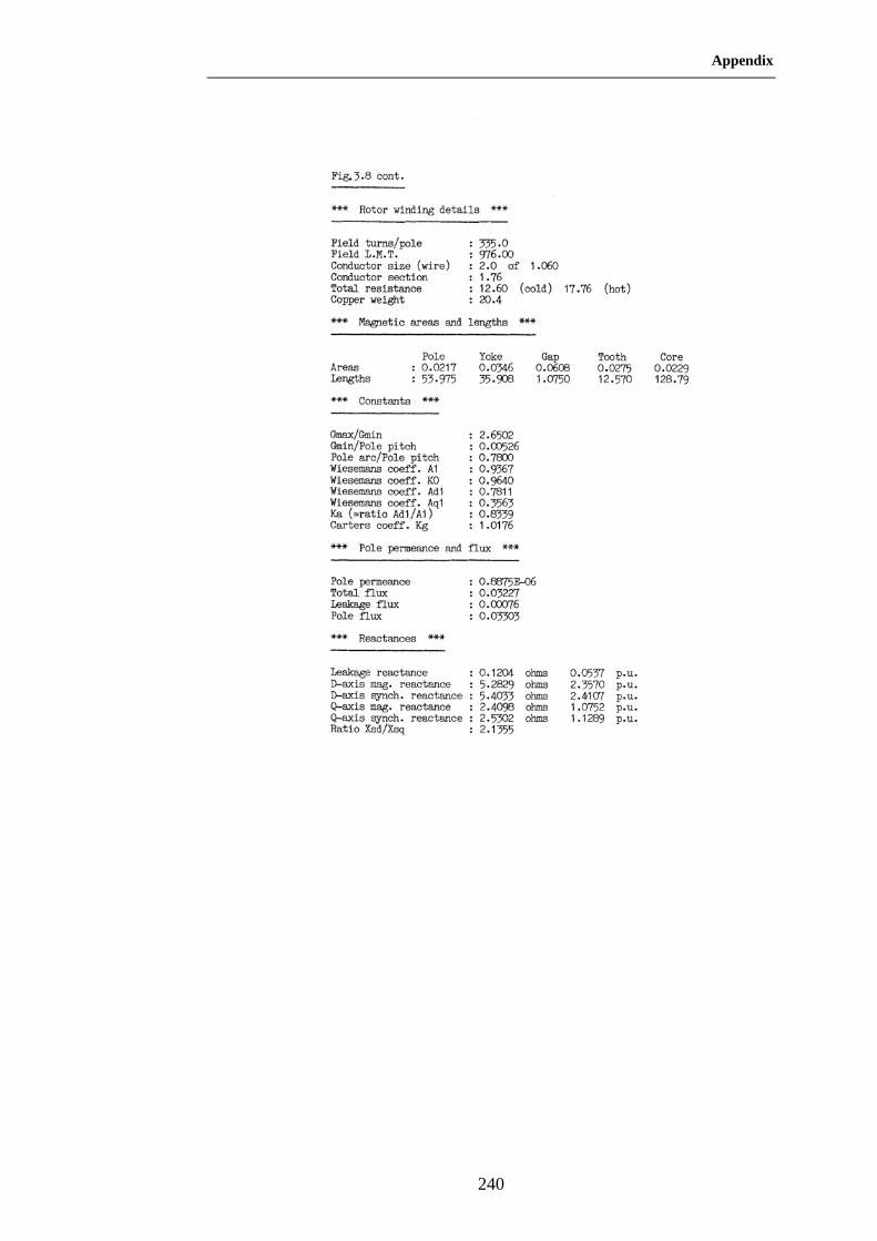
Appendix
240
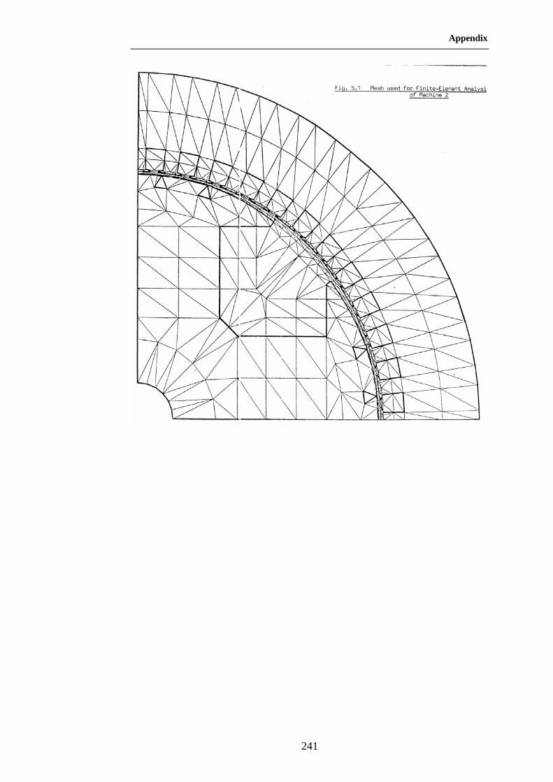
Appendix
241

References
242
REFERENCES
[1]: M.J. Carpenter, Magnetic Equivalent Circuits, Proceedings IEE, Vol. 115
(10), 1968, pp.1503-1511.
[2]: L. Haydock, The systematic development of equivalent circuits for
synchronous machines, Ph.d Thesis, University of London, 1986.
[3]: P. Sewell, K.J. Bradley, J.C. Clare, P.W. Wheeler, A. Ferrah, R. Magill,
Efficient dynamic models for induction machines, International Journal of
Numerical Modelling: Electronic Networks, Devices and Fields, (1999), Vol.
12, pp. 449-464.
[4]: J.L. Coulomb, G. Meunier, Finite element implementation of virtual work
principle for magnetic or electric force and torque computation, IEEE
Transactions on Magnetics, (1984), Vol. 20, No. 5, pp. 1894-1896.
[5]: J. Mizia, K. Adamiak, A. R. Eastham, and G. E. Dawson, Finite element
force calculation: Comparison of methods for electric machines, IEEE
Transactions on Magnetics, (1988), Vol. 24, No. 1, pp.447-450.
[6]: V. Ostovic', A method for evaluation of transient and steady state
performance in saturated squirrel cage induction machines, IEEE Transactions
on Energy Conversion, (1986), Vol. 1, No. 3, pp. 190-197.
[7]: V. Ostovic', A simplified approach to magnetic equivalent-circuit
modelling of induction machines, IEEE Transactions on Industry Applications,
(1988), Vol.24, No. 2, pp. 308-316.
[8]: V. Ostovic', A novel method for evaluation of transient states in saturated
electric machines, IEEE Transactions on Inustry Applications, (1989), Vol. 25,
No. 1, pp. 96-100.
[9]: M.J. Carpenter, D.C. Macdonald, Circuit representation of inverter-fed
synchronous motors, IEEE Transactions on Energy Conversion, (1989), Vol. 4,
No. 3, pp. 531-537.
[10]: H. Roisse, M. Hecquet, P. Brochet, Simulation of synchronous machines
using a electric-magnetic coupled network model, IEEE Transactions on
magnetics, (1998), Vol. 34, No. 5, pp. 3656-3659.
[11]: V. Ostovic', J.M. Miller, V.K. Garg, R.D. Schultz, S.H. Swales, A

References
243
magnetic-equivalent-circuit-based performance computation of a Lundell
alternator, IEEE Transactions on Industry Applications, (1999), Vol. 35, No. 4,
pp. 825-830.
[12]: Slides, Impact of excitation system on power system stability, ABB
Industrie AG.
[13]: Paul Breeze, Power generation technology, Elsevier, Oxford, 2005.
[14]: S. Smith, R. Todd, M. Barnes, P. Tavner, Improved energy conversion for
doubly-fed wind generators, IEEE annual meeting Industrial Application
Society (IAS), 2-6 October, 2005, Hong Kong.
[15]: M.G. Simoes, B.K. Bose, R.J. Spiegel, Fuzzy logic based intelligent
control of a variable speed cage machine wind generation system, IEEE
Transactions on Power electronics, (1997), Vol. 12, No. 5, pp. 87-95.
[16]: R. Datta, V.T. Ranganathan, Variable speed wind power generation using
doubly fed wound rotor induction machine-a comparison with alternative
schemes, IEEE Transactions on Energy Conversion, (2002), Vol. 17, No. 3, pp.
414-421.
[17]: S. Muller, M. Deicke, R.W. De Donker, Doubly fed induction generator
systems for wind turbines, IEEE Industry Applications Magzine, (2002),
May/June, pp. 26-33.
[18]: L. Morel, H. Godfroid, A. Mirzaian, J. Kauffmann, Double-fed induction
machine: converter optimisation and field oriented control without position
sensor, IEE Proceedings Electric Power Applications, (1998) vol. 145, No. 4,
pp. 360–368, July.
[19]: L. Xu and C. Wei, Torque and reactive power control of a doubly fed
induction machine by position sensorless scheme, IEEE Transactions on
Industry Applications, (1995) Vol. 31, No. 3, May/June, pp. 636–642.
[20]: B. Hopfensperger, D.J. Atkinson, Doubly-fed a.c. machines:
classification and comparsion, Proc. Power Electronics and Applications
(EPE), Graz, Austria, Aug., 27–29, 2001.
[21]: A.B.J. Reece, T.W. Preston, Finite element methods in electrical power
Engineering,
[22]: James L. Kirtley Jr., Electric Machines Lecture Notes, Massachusetts
Institute of Technology, Feburary 11, 2004.
[23]:W.H. Press, Saul A. Teukolsky, William T. Vetterling, Brian P. Flannery,

References
244
Numerical Recipes in C++: The Art of Scientific Computing, Cambridge
University Press, 2nd Edition, 2002.
[24]: A.E. Fitzgerald, Charles Kingsley, Jr., Stephen D. Umans, Electric
machinery, McGraw-Hill Higher Education, New York, 6th Edition, 2002.
[25]: P. L. Alger, Induction machines: their behaviour and uses, Gordon and
Breach, (1995), Basel, Switzerland.
[26]: K.J. Bradley, A. Tami, Reluctance mesh modelling of induction motors
with healthy and faulty rotors, 31st IEEE Industrial Application Conference,
San Diego, Oct. 6-10, 1996, pp.625-632.
[27]: Y. Saad, Iterative methods for sparse linear systems, PWS, Boston, 1996.
[28]: M.G. Say, Alternating Current Machines, Longman Science &
Technological, 5th edition, 1983.
[29]: Anisa, Ungku Anisa Ungku Amirulddin, Analysis and simulation of
vector controlled bearingless induction motors, Ph.d thesis, University of
Nottingham, 2005.
[30]: R.E. Steven, Electrical Machines and Power Electronics, Van Nostrand
Reinhold Co. Ltd, England, 1983.
[31]: F. Saccomanno, Electric power system analysis and control, IEEE Press
series on power engineering, Willey Interscience, 2003.
[32]: R.H. Park, Two-reaction theory of synchronous machines-generalized
methods of analysis-part 1, AIEE transaction, Vol. 48, July 1929, pp. 716-727.
[33]: J. Arrillaga, C. P. Arnold, Computer analysis of power systems, John
Wiley & Sons, 1990.
[34]: Stephen J. Chapman, Electric Machinery Fundamentals, 3rd Edition,
McGraw-Hill, 1998.
[35]: Peter P. Silvester, R.L. Ferrari, Finite Elements for electrical engineers,
3rd Edition, Cambridge University Press, 1996.
[36]: A. Darabi, C. Tindall, S. Ferguson, Finite-element time-step coupled
Generator, load, AVR, and brushless exciter modelling, IEEE Transactions on
Energy Conversion, (2004), Vol. 19, No. 1, pp. 73-80.
[37]: Ralph J. Smith, Richard C. Dorf, Circuits, devices and systems, 5th
Edition, John Wiley & Sons Inc.
[38]: Karl J. Astrom, Bjorn Wittenmark, Computer Controlled System Theory
and Design, Prentice-hall information and system sciences series, 1984.

References
245
[39]: Norman S. Nice, Control System Engineering, 4th Edition, John Wiley &
Son, 2004, New York.
[40]: Charles L. Phillips, H. Troy Nagle, Digital control system analysis and
design, 2nd Edition, Prentice-Hall International, 1990.
[41]: J. Machowski, J.W. Bialek, S. Robak, J.R. Bumby, Excitation control
system for use with synchronous generators, IEE Proceedings, Generation,
Transmission and Distribution., Vol. 145, No.5, September 1998.
[42]: A. Darabi, C.E. Tindall, Analogue AVR model for use in real time
transient simulation of small salient pole alternators, Power electronics,
machines and drives, Conference Publications No. 487, 16-18 April 2002,
IEE2002
[43]: P.M. Anderson, A.A. Fouad, Power system control and stability, IEEE
Press, 2nd edition, 2002.
[44]: M.L. Crenshaw et al., Excitation system models for power system
stability studies, IEEE committee report, IEEE transactions on power
apparatus and system, Vol. PAS-100, No. 2 February 1981.
[45]: R. C. Shaw, Modelling and Simulating Automatic Voltage Regulators for
Newage AVK SEG Generators, MENG Hons Project Report Part 2 HSP 1876
[46]: Kiyong Kim, Richard C. Schaefer, Tuning a PID Controller for a Digital
Excitation Control System, IEEE Transactions on Industry Applications, Vol.
41, No. 2 March/April 2005.
[47]: A. Godhwani, M.J. Basler, K. Kim, T.W. Eberly, Commissioning
Experience with a Modern Digital Excitation System, IEEE Transactions on
Energy Conversion, Vol. 13, No. 2 June 1998.
[48]: M.G. McArdle, D.J. Morrow, P.A.J. Calvert, O. Cadel, Implementation of
a Digital AVR for Small Alternators, Proceedings of International Conference
on Electric Utility Deregulation and Restructuring and Power Technologies,
City University, London, 4-7 April 2000.
[49]: Danish wind industry association, information available at:
http://www.windpower.org/en/news/articles
[50]: Anderson Peterson, Analysis, Modelling and Control of Doubly-fed
Induction Generators for Wind Turbines, Ph.D thesis in Chalmes University of
Technology, Goteborg, Sweden, 2005.
References
246
[51]: A. Miller, E. Muljadi, and D. S. Zinger, a variable speed wind turbine
power control, IEEE. Trans. Energy Conversion, vol. 12, pp. 181-187, June
1997.
[52]: http://www.istis.sh.cn/list/list.asp?id=1980
[53]: http://www.repower.de/index.php?id=12&L=1
[54]: B. Hopfensperger, D.J.Atkinson, R.A. Lakin, Stator flux oriented control
of a cascaded doubly-fed induction machine, IEE proceedings Electric Power
Application, vol. 146, No.6, November 1999.
[55]: B. Hopfensperger, D.J.Atkinson, R.A. Lakin, combined magnetising flux
oriented control of the cascaded doubly fed induction machine, IEE
proceedings Electric Power Application, vol. 148, No.4, July 2001.
[56]: [F-7]: B. Hopfensperger, D.J.Atkinson, R.A. Lakin, The application of
field oriented control to a cascaded doubly fed induction machine, Power
Electronics and Variable Speed Drives, 18-19 September 2000, Conference
Publication No. 475.


![GATOR PNEUMATIC MAGNETIC DRILLING MACHINE UNDERWATER … · GATOR PNEUMATIC MAGNETIC DRILLING MACHINE UNDERWATER USE Model ... Mounting of cutters [5] ... Attach an additional piece](https://static.fdocuments.in/doc/165x107/5ae1b18d7f8b9ae74a8b8bf7/gator-pneumatic-magnetic-drilling-machine-underwater-pneumatic-magnetic-drilling.jpg)