Pavia, 2011 1

Symbolic Methods and AceGen

Jože KorelcUniversity of Ljubljana, Slovenia

Mercator Visiting Professor at Leibniz Universität Hannover

Pavia, 2011 2

Computational Solution Environments

• General problem solving environment (PSE)– general solvers for ODE‐s or PDE‐s– user templates are provided for certain class of problems ‐

ELLPACK, DIFPACK, SCIRun, FlexPDE– numerical libraries with compiled functions ‐ NAG– interactive numerical environments ‐MATLAB, FEMLAB– symbolic systems Mathematica, Maple

• Object oriented environments– collection of objects, clases, methods– DIFPACK, FEMTheory

• Specialized finite element enviroments– ABAQUS, FEAP, ANSYS, ...

• Hybrid approaches

Pavia, 2011 3

Hybrid approaches

• Steering application provides interfaces to the tools– Alice, SCIRun– popular for multi‐physics, multi‐field

• Hybrid object‐oriented approach– domain‐specific language– built‐in C++ libraries for symbolic manipulation and AD– FeniCS, FreeFem++

• Hybrid symbolic–numeric approach– general computer algebra system for code generation– general finite element environment– AceGen, AceFEM

Pavia, 2011 4

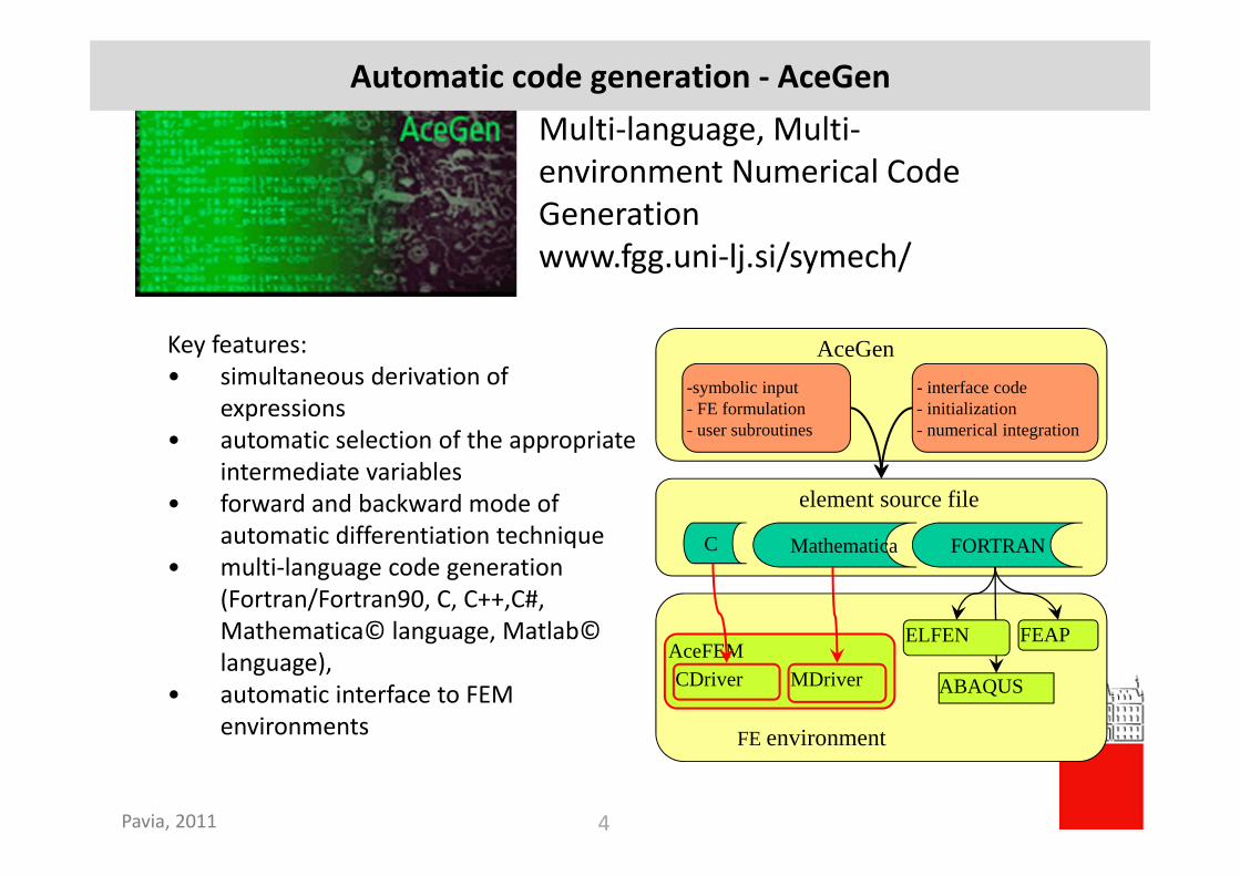
Multi‐language, Multi‐environment Numerical Code Generationwww.fgg.uni‐lj.si/symech/

Key features:• simultaneous derivation of

expressions• automatic selection of the appropriate

intermediate variables• forward and backward mode of

automatic differentiation technique• multi‐language code generation

(Fortran/Fortran90, C, C++,C#, Mathematica© language, Matlab© language),

• automatic interface to FEM environments

C FORTRANMathematica

element source file

AceFEMCDriver

FEAPELFEN

MDriver ABAQUS

FE environment

AceGen-symbolic input- FE formulation- user subroutines

- interface code- initialization- numerical integration

Automatic code generation ‐ AceGen

Pavia, 2011 5

<< AceGen`;SMSInitialize@"filename",

"Language" −> "Mathematica"D;SMSModule@"Gradf", Real@u$$@3D, x$$, L$$, g$$@3DDD;8x, L< ¢ 8SMSReal@x$$D, SMSReal@L$$D<;uh ¢ SMSReal@Table@u$$@iD, 8i, 3<DD;

Nh £ 9x

L, 1 −

x

L,x

L1 −

x

L=;

u £ Nh.uh;

f £ u2;

g £ SMSD@f, uiD;SMSExport@g, g$$D;SMSWrite@D;

Multi‐language code generation

1. Mathematical description

3. Automatically generated code

SUBROUTINE Test(v,u1,x,L,g)REAL*8 v(500),u1(3),x,L,g(3)v(6)=x/Lv(7)=1d0 - v(6)v(8)=v(6)*v(7)v(12)=2d0*(u(1)*v(6) +

- u(2)*v(7) + u(3)*v(8))g(1)=v(12)*v(6)g(2)=v(12)*v(7)g(3)=v(12)*v(8)END

"Fortran"

3

1

2

ˆ ˆ

ˆ ,1 , (1 )

?

i ii

u N u

x x x xL L L L

f u

f

=

=

= − −

=∇ =

∑

N

void Test(double v[501],double u1[3],double *x,double *L,double g[3])v[6]=*x/*L;v[7]=1e0 - v[6];v[8]=v[6]*v[7];v[12]=2e0*(u[0]*v[6] +u[1]*v[7]+ u[2]*v[8]);

g[0]=v[12]*v[6];g[1]=v[12]*v[7];g[2]=v[12]*v[8];;

"C++"Test[]:=Module[,$VV[6]=x$$/L$$;$VV[7]=1 - $VV[6];$VV[8]=$VV[6]*$VV[7];$VV[12]=2*(u$$[1]*$VV[6] +

u$$[2]*$VV[7]+u$$[3]*$VV[8]);g$$[1]=$VV[6]*$VV[12];g$$[2]=$VV[7]*$VV[12];g$$[3]=$VV[8]*$VV[12];]

"Mathematica"

"Fortran""C""Mathematica"

Pavia, 2011 6

Multi‐environment code generation

FEAP AceFEM

subroutine elmt10(d,ul,xl,ix,tl,s,p,& ndfe,ndme,nste,isw)implicit noneinclude 'sms.h'logical DEBUG,symmetriccharacter*50 SELEM,datades(0),postdes(0)parameter (DEBUG=.false.,.....End

SUBROUTINE SKR10(v,d,ul,ul0,xl,s,p,ht,hp)IMPLICIT NONEinclude 'sms.h'DOUBLE PRECISION v(5001),d(0),ul(2,4),& ul0(2,4),xl(2,4),s(8,8),p& (8),ht(*),hp(*)s(1,1)=1d0END

#include "sms.h"void SKR(double v[501],ElementSpec *es,ElementData *ed,NodeData **nd,double *rdata,int *idata,double*p,double **s);__declspec(dllexport) void SMTSetElSpec(ElementSpec *es,int *idata,int *ic,double *gd) static int pn[5]=1, 2, 3, 4, 0; static int dof[4]=5, 5, 5, 5; static char *gdcs[]="Const 1","Const 2"; static char *gpcs[]="";static char *npcs[]=""; es->Code="test";es->id.NoDimensions=2;es->id.NoDOFGlobal=20; es->id.NoDOFCondense=0;es->id.NoNodes=4; es->id.NoGroupData=2;es->id.NoSegmentPoints=5; es->id.IntCode=*ic;es->id.NoElementData=0; es->Segments=pn;es->DOFGlobal=dof;es->Data=gd; es->id.NoGPostData=0;es->id.NoNPostData=0; es->id.SymmetricTangent=1; es->IntPoints=SMTIntPoints(ic);es->id.NoTimeStorage=0; es->Topology="Q1";es->GroupDataNames=gdcs; es->GPostNames=gpcs;es->NPostNames=npcs;es->user.SKR=SKR;;

void SKR(double v[501],ElementSpec *es,ElementData *ed,NodeData **nd,double*rdata,int *idata,double *p,double **s)p[0]=nd[0]->X[0];;

<<AceGen`;SMSInitialize["test",

"Environment"→"AceFEM"];SMSTemplate["SMSTopology"→"Q1"];SMSStandardModule["Tangent and residual"];SMSExport[1,s$$[1,1]];SMSWrite[];

<<AceGen`;SMSInitialize["test",

"Environment"→"FEAP"];SMSTemplate["SMSTopology"→"Q1"];SMSStandardModule["Tangent and residual"];SMSExport[1,s$$[1,1]];SMSWrite[];

Suplementaryroutines

usersubroutines

Pavia, 2011 7

Mathematica

Expression optimization

Pavia, 2011 8

Simultaneous optimization of the expressions

• expressions are optimize immediately after they are derived• special procedures are needed for non-local operations• appropriate for large problems where also intermediate results

can be subjected to the uncontrolled swell of expressions

Original matrixResult is optimized matrix, expressed with the new auxiliary variables

Vector of 7 new auxiliary variables:

63 2

33 3

1 2 1 2 1 212 6 4, ,

2, , , ,

v v v v v vE I

vLv

vv v

⎧ ⎫⎪ ⎪⎪ ⎪= ⎨ ⎬−⎪ ⎪⎪ ⎪⎩ ⎭

4 5 4 5

5 6 5 70

4 5 4 5

7 65 5

v v v v

v v v v

v v v v

v vv v

⎡ ⎤⎢ ⎥⎢ ⎥−⎢ ⎥= ⎢ ⎥− −⎢ ⎥⎢ ⎥− ⎥⎦

−

−

⎢⎣

K

3 2 3 2

2 2

3 2 3 2

2

0

2

12 6 12 6

6 4 6 2

12 6 12 6

6 2 6 4

EI EI EI EI

L L L LEI EI EI EI

L LL LEI EI EI EI

L L L LEI EI EI EI

L LL L

⎡ ⎤⎢ ⎥⎢ ⎥⎢ ⎥⎢ ⎥⎢ ⎥⎢ ⎥= ⎢ ⎥⎢ ⎥⎢ ⎥⎢ ⎥⎢ ⎥⎢ ⎥⎢ ⎥⎣ ⎦

− − −

−

−

−

K

AceGen

Optimized matrix

Pavia, 2011 9

Automatic theorem provingHow to prove arbitrary (mathematical) statement automatically ?

KKKIKK

1

1

2=•

=•−

−

//Automatic theorem proving is essential when large expressions derived by a symbolic system need to be simplified.

General symbolic matrices A and B:

Pavia, 2011 10

Deterministic methods

• general solution is not available• statements that can be expressed as a system of algebraic

equations– statement is correct if the corresponding system of algebraic equations has a

solution– Grobner bases

• technique provides algorithmic solution to a system of algebraic (polynomial) equations• Grobner bases are computed by the Buchberger´s algorithm• Buchberger´s algorithm is equivalent to Gauss elimination for the system of polynomial equations

• Mathematica

Pavia, 2011 11

• Numerical identification of relations between expressions– the simplest way of automatic theorem proving– the problem of equivalence testing is determining whether two

expressions (different in appearance) are indeed mathematically the same.

• The correctness can be numerically determined only with a certain degree of probability

Heuristic methods

?0)1)(1(1)( 5510 =+−+−= xxxxf022)( 5 ≠−= xxf

x^10 − 1 + H1 − x^5L Hx^5 + 1L êê Expand0

x^10 − 1 + H1 − x^5L Hx^5 + 1L ê. x → RandomReal@D−1.11022×10−16

Pavia, 2011 12

Signature functions

Possible signature functions:1. every expression is mapped into an integer of arbitrary length

– complex implementation– general method

2. every expression is evaluated with the set of real randomnumbers of arbitrary precission

Numerical identification of relations between set of expressions

1 1

2 2 1

1 1

0 :

1 : ( )

2 : ( , )

....

: ( , ,..., )n n n

x

y f x

y f x y

n y f x y y −

==

=

0

1 0

2 0 1

1 2 1

0 : ( ) ...

1 : ( )

2 : ( , )

....

: ( , , )n n

S S x randomsignature

S S S

S S S S

n S S S S S −

===

=

⎩⎨⎧

≡⇒=≠⇒≠

=−jk

jkjk yy

yySS

00

with a probability that canbe tuned

Pavia, 2011 13

Heuristic code optimization

Probability of wrong simplification is for this case is defined by:

• probability that polynomial equation has roots on interval

• floating point precision

- 4 - 2 2 4

- 5

5

10

15

critical x where simplification fails]4,4[

||

12

2

231

−∈+=

+−=

xxxf

xxf

Example 1:

Pavia, 2011 14

Mathematica

Auxiliary variables

Pavia, 2011 15

Assignment operators

<< AceGen`;SMSInitialize@"test",

"Language" −> "Mathematica"D;SMSModule@"test", Real@x0$$, r$$DD;x0 ¢ SMSReal@x0$$D;x • x0;

SMSDoBf £ x2 + 2 SinAx3E;

dx £ −f

SMSD@f, xD;

x § x + dx;SMSIf@Abs@dxD < 10^−10,SMSBreak@D;D;

SMSIf@i == 15, SMSReturn@D;D;

, 8i, 1, 30, 1, 8x<<F;SMSExport@x, r$$D;SMSWrite@D;

Four additional assignment operators in AceGenreplace the standard Mathematica assignment operator lhs=rhs

General algorithm

Pavia, 2011 16

SMSIf@x ≥ 0Dy • x2;SMSElse@D;y § Sin@xD;SMSEndIf@yD;

"If" construct

Conditional statements

auxiliary variable 3y ($V[i,3])

auxiliary variable 1y ($V[i,1])

auxiliary variable 2y ($V[i,2])

2 0

( ) 0

x xy

Sin x x

⎧⎪ ≥⎪= ⎨⎪ <⎪⎩

y = IfAx ≥ 0

, x2

, Sin@xDE

y £ SMSIfAx ≥ 0

, x2

, Sin@xDE

Mathematica input

In-cell AceGen input

Cross-cell AceGen input

Pavia, 2011 17

y • 0;SMSDo@ i, 1, n, 1, yD;y § y + xi;SMSEndDo@yD

• "Do" construct

Loops

1

ni

i

y x=

= ∑Mathematica input

In-cell AceGen input

Cross-cell AceGen input

1y2y

3y

4y

y = 0; n = 10;

DoAy = y + xi;, 8i, 1, n, 1<

E;

y • 0;

SMSDoAy § y + xi;, 8i, 1, n, 1, y<

E;

Pavia, 2011 18

Automatic Differentiation

Pavia, 2011 19

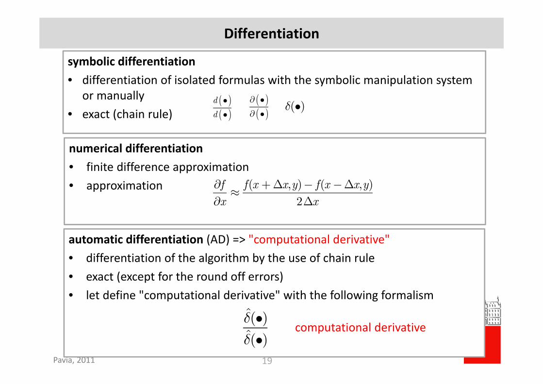
Differentiation

numerical differentiation• finite difference approximation• approximation ( , ) ( , )

2f f x x y f x x yx x

∂ +Δ − −Δ≈

∂ Δ

automatic differentiation (AD) => "computational derivative"• differentiation of the algorithm by the use of chain rule• exact (except for the round off errors)• let define "computational derivative" with the following formalism

( )

( )

δδ••

symbolic differentiation• differentiation of isolated formulas with the symbolic manipulation system

or manually• exact (chain rule)

( )( )

∂ •

∂ •( )( )d

d

•

•( )δ •

computational derivative

Pavia, 2011 20

Automatic differentiation

• Automatic differentiation technique (AD):– differentiation of the whole program– automatic differentiation tool generates a program code for the

derivative from a program code for the basic function– control structures (If, Do,..) are left unchanged

• Two basic methods of AD:– forward mode of AD

• standard "chain rule" on a level of the algorithm

– backward mode of AD• also named: reverse mode, inverse method, adjoint code construction, adjoint sensitivity, ....

Pavia, 2011 21

Forward versus backward mode

2

1

1 :

2 : ( )

3 :

l

n

l

b x

c Sin b

y bc

=

=

==

∑

2 ; 1,2,...,

( ) ; 1,2,...,

; 1,2,...,

ll

ll

l ll

dbb x l n n

dxdc

c Cos b b l n ndxdy

y b c b c l n ndx

⎧ ⎫⎪ ⎪⎪ ⎪∇ = = =⎨ ⎬⎪ ⎪⎪ ⎪⎩ ⎭⎧ ⎫⎪ ⎪⎪ ⎪∇ = = ∇ =⎨ ⎬⎪ ⎪⎪ ⎪⎩ ⎭⎧ ⎫⎪ ⎪⎪ ⎪∇ = = ∇ + ∇ =⎨ ⎬⎪ ⎪⎪ ⎪⎩ ⎭

1 1

1

( ) 1

2 ; 1, 2, ...,l ll l

dyy

dydy y

c y b ydc cdy y c

b y c cy Cos b cdb b bdy b

y x b x b l n ndx x

= =

∂= = =

∂∂ ∂

= = + = +∂ ∂

⎧ ⎫ ⎧ ⎫⎪ ⎪ ⎪ ⎪∂⎪ ⎪ ⎪ ⎪∇ = = = = =⎨ ⎬ ⎨ ⎬⎪ ⎪ ⎪ ⎪∂⎪ ⎪ ⎪ ⎪⎩ ⎭ ⎩ ⎭

forward mode

2

1

1 :

2 : ( )

3 :l

n

l

y bc

c Sin b

b x=

==

= ∑

vector of independentvariables y( ) dependent variable y=?n− − ∇x x

- adjoint values, ,y c breversal of the flow of the program

backward mode

Pavia, 2011 22

Efficiency of automatic differentiation

• wratio(f) ‐ work ratio

• cost(f) ‐ the number of arithmetic operations for evaluating f

• cost(f,∇f) ‐ the number of arithmetic operations for evaluating f and it´s gradient with n components

cost( , )( )

cost( )f f

wratio ff∇

=

backward mode• "If care is taken in handling quantities which are common to the function

and derivative, the cost ratio is usually around 1.5, not n+1" (Wolfe, 1982)

• formal proof by Baur and Strassen (1983) ( ) 5wratio f <

forward mode

• Computational cost proportional to n ( ) ( 1)wratio f nα≈ +

Pavia, 2011 23

Implementation of AD

• Source‐to‐source translator– original source is transformed into derivative code– compile‐time solution– ADIFOR, Odyssee, TAMC– minimal changes in original code (declaration of input and output

variables)

• Operator overloading– modern compilers accept user‐defined data types and operator

overloading– run‐time solution– low numerical efficiency– ADOL‐C

( )a b a b+ ⇒ ∇ +

Pavia, 2011 24

Automatic differentiation in AceGen

AceGen enhancements with respect to the standard ADtechnique:

• AD procedure can be initiated at any time and at any point andas many times as required within the same user subroutine

• AD as code‐to‐code translator consistently extends currentcode rather than produce a new one

• the results of all previous uses of AD have to be accounted forwhen AD is used several times

• mechanism to include exceptions within the AD procedureeasily

Pavia, 2011 25

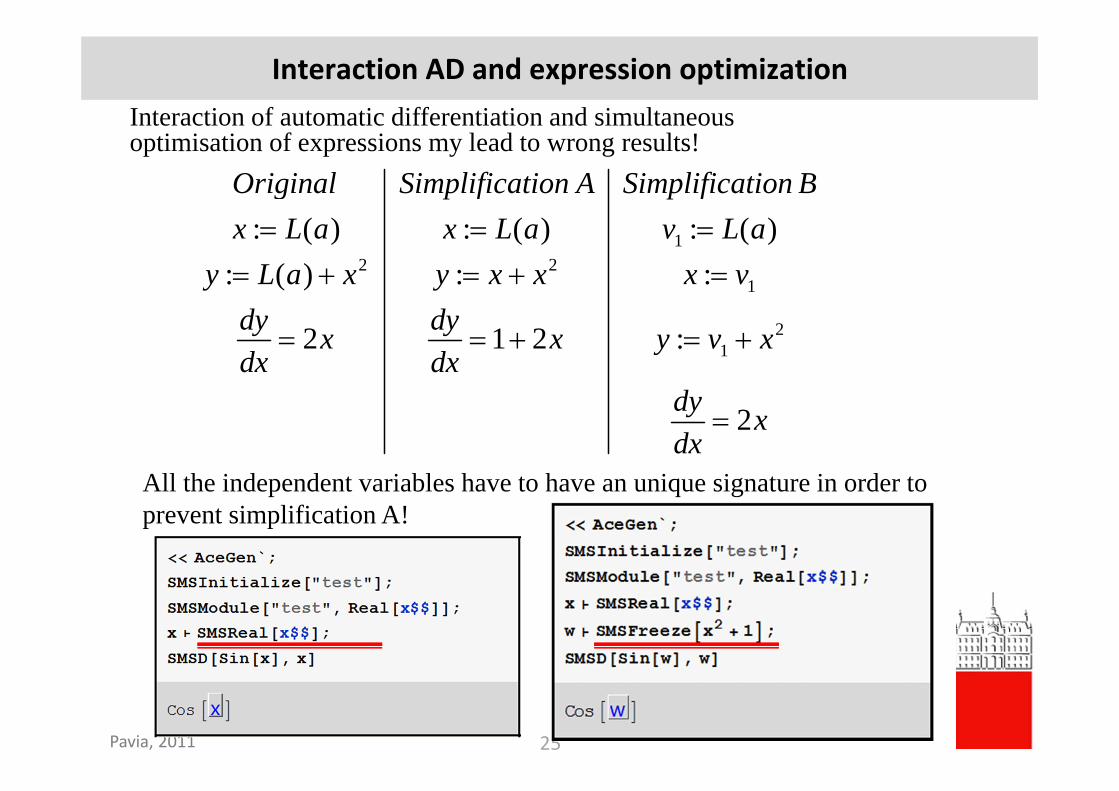
Interaction AD and expression optimizationInteraction of automatic differentiation and simultaneousoptimisation of expressions my lead to wrong results!

12 2

1

21

: ( ) : ( ) : ( ): ( ) : :

2 1 2 :

2

Original Simplification A Simplification Bx L a x L a v L a

y L a x y x x x vdy dyx x y v xdx dx

dy xdx

= = == + = + =

= = + = +

=

All the independent variables have to have an unique signature in order to prevent simplification A!

Pavia, 2011 26

• How to translate mathematical formalisms into AD procedure?• partial, total, directional, Lee, covariant, consistent, …• various notations

• Extended automatic differentiation technique (Korelc, 2002)• Control of "exceptions" in AD is crucial to relate to mathematical

formalisms

Automa c differen a on Exceptions

AD produces values of derivatives of what is actually computed, rather than what one intends to compute.

( )( )

∂ •∂ •

( )( )

DD

••

( )δ •

Pavia, 2011 27

AD Exception

Formalism for introduction of AD exceptions

... independent variables

... intermediate variables

( , ( )) ... function

... arbitrary matrix

ˆ ( , ( )): ˆ D

D

f

ff

δδ =

∇ =bM

a

aba b aM

a b aa

( , ( ))f a b a

a

b

program flow

back propagation of AD adjoints

DD

=b

Ma

f∇

definitionof AD exceptions

f £ SMSD@f@a, bD, a, "Dependency" → 8b, a, M<DAceGen input - option "Dependency"

Pavia, 2011 28

Local/Global definition of AD exception

• Local AD exception– AD exception is introduced when AD procedure is executed

• Global AD exception– AD exception is introducued together with intermediate

variables b

: ( )

ˆ ( , ( )): ˆ

DD

Af

fδ

δ

==

∇ =

bM

ab G a

a b aa

ˆ ( , ( )): ˆA

DD

ff

δδ =

∇ =bM

a

a b aa

a ¢ SMSReal@a$$Db ¢ SMSFreeze@G@aDDf £ SMSD@f@a, bD, a, "Dependency" → 8b, a, M<D

a ¢ SMSReal@a$$Db ¢ SMSFreeze@G@aD, "Dependency" → 8a, M<Df £ SMSD@f@a, bD, aD

Pavia, 2011 29

Types of AD exception

The basic situations that have to be considered are:A. Basic case: The total derivatives of intermediate variables a with respect to

independent variables b are set to be equal to matrixM.

B. Special case: There exists explicit dependency between variables that has to be neglected for the differentiation

C. Implicit case: There exists implicit dependency between variables that has to be considered for the differentiation

D. Generalization: The total derivatives of intermediate variables a with respect to intermediate variables c are set to be equal to matrixM.

ˆ ( , ( )):

( )BDD

ff

δδ =

∇ =b0

a

a b aa

ˆ ( , ( ( ))):

ˆDDD

ff

δδ =

∇ =bM

c

a b c aa

ˆ ( , ( )):

ˆADD

ff

δδ =

∇ =bM

a

a b aa

ˆ ( , ):

ˆCDD

ff

δδ =

∇ =bM

a

a ba

Pavia, 2011 30

• AD can "see" only explicit dependencies!

• implicit dependency between variables has to be specified as exception in AD

AD Exception Type C

a

bAD exception

DD

=b

Ma

back propagation of AD adjoints

( )f b

program flow

ˆ ( , ): ˆ D

D

ff

δδ =

∇ =bM

a

a ba

f∇

Pavia, 2011 31

Nonlinear mapping from reference coordinates to initial coordinates in FEM

Example ‐ exception Type C

, , reference coordinates

( ) ( ) actual coordinates

( ) ( ) displacements

displacement gradient

k kk

k kk

N

N

ξ η ζ==

=

∂=

∂

∑∑

X X

u u

uX

ΞΞ Ξ

Ξ Ξ

H

ˆ ( ): 0 wrong AD formulationˆ ( )

δδ

= =ΞΞ

uH

X

correct AD formulation1( )

ˆ ( ): 0ˆ D

D

δδ −⎡ ⎤∂⎢ ⎥=⎢ ⎥∂⎣ ⎦

= ≠X

XΞ Ξ

Ξ

ΞuH

X

ADB notationautomatic differentiation based notation

SMSD[u,X,"Dependency"->Ξ,Inverse[SMSD[X,Ξ]]

Higher level symbolic language (Mathematica + AceGen)

Pavia, 2011 32

ADB form and AceFEM

Pavia, 2011 33

Finite element solution procedure

1. strong form of boundary‐value problem2. weak form

3. FE approximation of field variables4. enforcement of local constraints5. element quantities (K, R, …)6. programming of steps 3, 4,5

7. generation of mesh and boundary conditions8. contact search algorithm9. solution of the global problem10. presentation and analysis of results

Automation of formulationat the individualelementlevel

( )

( )

( ) 0

...

1...

2

T

T

k Q

k Q d

k d

φ

δ δφ φ δφ

φ φ

Ω

Ω

∇ ∇ + =

Π = ∇ ∇ − Ω −

Π = ∇ ∇ Ω −

∫

∫

,

i i

ii

ii j

j

N

R

RK

φ φ

φ

φ

=∂Π

=∂∂

=∂

Pavia, 2011 34

ADB Notation

• ADB (Automatic Differentiation Based) form of computational model

• ADB form bridges mathematical notation of computational models and actual computer implementation.

• ADB form can be directly translated into the program code and the derived program code is numerically efficient.

The unification of the classical mathematical notation of computational models and the actual computer implementation can be achieved by means of automatic differentiation combined with the automatic code generation.

Automatic differentiation+ AD exceptions

ADB(Automatic Differentiation Based) form of computational model

Pavia, 2011 35

Problem is defined by:• Hyperelastic strain energy function

• FE approximation of coordinates and displacements– Nonlinear mapping from reference coordinates to initial coordinates

Example: 3D hyperelastic element

, , reference coordinates

( ) ( ) actual coordinates

( ) ( ) displacements

k kk

k kk

N

N

ξ η ζ==

=

∑∑

X X

u u

ΞΞ Ξ

Ξ Ξ

ˆ ( ): 0 wrong ADB notationˆ ( )

δδ

= =ΞΞ

nH

X

1( )

ˆ ( ): 0ˆ D

D

δδ −⎡ ⎤∂⎢ ⎥=⎢ ⎥∂⎣ ⎦

= ≠X

XΞ Ξ

Ξ

ΞuH

X

Higher level symbolic language (Mathematica + AceGen)

2( 3)

( 1) ( ( ))2 2

trW det Log det

λμ

−= − + −

= +∂∂

I

CF F

F Hu

H =X

SMSD[u,X,"Dependency"->Ξ,Inverse[SMSD[X,Ξ]]

Automation

Pavia, 2011 36

ADB form: Hyperelastic material ‐ A1 2 , ,..., vector of elements generalized d.o.f.

W( ) hyperelastic strain energy function

the contribution of the e-th element to the global residual

integration point contribution of the resid

e n

e

e

g

p p p=pp

RR ual of the e-th element

ˆ ( ): ˆ

eg g

e

WJ

δ

δ=

pR

p

(A) Solution is a stationary point of the hyperelastic potential

( )eg g

e

WJ

∂=

∂p

Rp

Automation

e g gg

w= ∑R R

int

e e

e W dV WdVδΩ Ω

Π = →∫ ∫

( )

e

T Tee g g e g g

g ge

WWdV J w wδ δ δ

Ω

⎡ ⎤ ⎡ ⎤⎛ ⎞∂ ⎟⎜⎢ ⎥ ⎢ ⎥⎟≈ =⎜ ⎟⎢ ⎥ ⎢ ⎥⎜ ⎟⎜ ∂⎝ ⎠⎢ ⎥ ⎢ ⎥⎣ ⎦ ⎣ ⎦∑ ∑∫

pp p R

p

int 0ext δΠ = Π + Π → Π =

Pavia, 2011 37

ADB form: Hyperelastic material ‐ B

(B) Virtual work principle

( )int

e

e g gg

dV J wδ δ δΩ

Π = ⋅ ≈ ⋅∑∫ P F P F

( )eg g

e

J∂

= ⋅∂

F pR P

p

( )ee

e

δ δ∂

=∂

F pF p

p

ˆ: ˆWδδ

=PF

int 0extδ δ δΠ = Π + Π =

W∂=

∂P

F

( )int eT Te e g g e g g

g ge

J w wδ δ δ⎡ ⎤ ⎡ ⎤∂⎢ ⎥ ⎢ ⎥Π ≈ ⋅ =⎢ ⎥ ⎢ ⎥∂⎢ ⎥ ⎢ ⎥⎣ ⎦ ⎣ ⎦∑ ∑

F pp P p R

p

Automation

ˆ: ˆg g

e

Jδδ

= ⋅F

R Pp

Pavia, 2011 38

Numerical cost : Hyperelastic material

backward mode AD

cost( ) (cost( ) 9cost( ))g Wα≈ +R F

(B) Virtual work principle

ˆ: ˆWδδ

=PF

ˆ ( ): ˆ

eg g

e

WJ

δ

δ=

pR

p

(A) Solution is a stationary point of the hyperelastic potential

backward mode AD

cost( ) cost( )g Wα≈R

1.5 5α< <optimal ADB form

ˆ: ˆg g

e

Jδδ

= ⋅F

R Pp

Pavia, 2011 39

Algorithm for primal analysis of hyperelastic problems

(0)0; ni = =p p

( ) ( ) ( ) ( ) ( )( )

( )( ) ( ) ( ) ( ) ( )

( )

; ;

; ;

i i i i ig e g g g ei

g eeigi i i i i

g e g g g eig ee

Ww J

w J

∂= = =

∂∂

= = =∂

∑

∑

R R R R RpR

K K K K Kp

AA

( 1)1

in

++ =p p

No( )i TOL<R

i:=i+1

Yes incn n<

No

Yes

00; initialn = =p p

( ) ( ) ( ) ( )

( 1) ( ) ( )

i i i i

i i i+

Δ = − → Δ

= + Δ

K p R p

p p p

Yes

Newton-Raphson scheme for nonlinear hyperelastic problemssubjected to quasi-static proportional loadwith constants load stepping Automation of the scheme

(0): 0; : ; :n ni λ λ λ= = = + Δp p

( ) ( ) ( ) ( ) ( )( )

( )( ) ( ) ( ) ( ) ( )

( )

ˆ: ; : ; :

ˆˆ

: ; : ; :ˆ

i i i i i refg g e g g ei

g eeigi i i i i

g e g g eig ee

WJ w

w

δλ

δδ

δ

= = = −

= = =

∑

∑

R R R R R Rp

RK K K K K

p

AA

( 1)1 1: ; :i

n nλ λ++ += =p p

No( )i TOL<R

i:=i+1

Yes

No

n:=n+1

Yes

0

0

: 0; :

: 0; : 1initial

inc

n

nλ λ= == Δ =p p

( ) ( ) ( ) ( )

( 1) ( ) ( ):

i i i i

i i i+

Δ = − → Δ

= + Δ

K p R p

p p p

Yes

incn n<

(0)0; ;n ni λ λ λ= = = + Δp p

( ) ( ) ( ) ( ) ( )( )

( )( ) ( ) ( ) ( ) ( )

( )

; ;

; ;

i i i i i refg g e g g ei

g eeigi i i i i

g e g g eig ee

WJ w

w

λ∂

= = = −∂

∂= = =

∂

∑

∑

R R R R R Rp

RK K K K K

p

AA

( 1)1 1;i

n nλ λ++ += =p p

No( )i TOL<R

i:=i+1

Yes incn n<

No

Yes

0

0

0;

0; 1initial

inc

n

nλ λ= == Δ =p p

( ) ( ) ( ) ( )

( 1) ( ) ( )

i i i i

i i i+

Δ = − → Δ

= + Δ

K p R p

p p p

Yes

n:=n+1

Pavia, 2011 40

Model: elasto‐plastic theory that assumes elastic isotropic responsedefined by the additive decomposition of strain tensor

• vector of element d.o.f. • vector of unknown state variables g ‐ Gauss point• elastic strain• elastic free energy function per unit volume • yield function• evolution equations for

• Q ‐ set of additional set of algebraic equations per Gauss point that has to be solved for unknown hg

• Solution: local Newton‐Raphson iterations at Gauss point– consequence: dependency of state variables on displacement

Small strain plasticity ‐ definitions

,pg mε λ=hep

pe = −ε ε ε

W=W( )eε

3 1 1( ) tr( ) : tr( )

2 3 3 yf σ σ σ σ σ σ⎛ ⎞ ⎛ ⎞⎟ ⎟⎜ ⎜= − − −⎟ ⎟⎜ ⎜⎟ ⎟⎜ ⎜⎟ ⎟⎝ ⎠ ⎝ ⎠

0p p pn

pmf

ε

ε λ

− −Δ∂

Δ

=

=∂

ε ε

σ

0p p p

n

f

ε⎧ ⎫⎪ ⎪⎪ ⎪ =⎨ ⎬− −

⎪ ⎪⎪ ⎪

Δ

⎩ ⎭Q =

ε ε

pε

( )g eh p

Pavia, 2011 41

ADB form of small strain plasticity

Virtual work:

( ) 0trialf ≥σ

ˆ ( , ): ˆ

g nWδ

δ=

hεσ

ε( ) 0trialf <σ

,

0

ˆ ( , , ): ˆ

g

e

g g n

D

D

Wδ

δ=

=h

p

h hεσ

ε

0

ˆ: ˆ

g

e

g g DeD

WJ

δδ =

=h

p

Rp

( ) 1ˆ

ˆ

ˆ: ˆ

g gg

e e

gg

DeD

δ

δ

δ

δ −=−

=h Q

Ap p

RK

p

ˆ: ˆg

e

δδ

= ⋅Rpεσ

efficient form of consistent linearization(dependency due to the local NR loop)

suppress implicit dependencydue to the local NR loop

ADB form of plasticity problems

0 0

ˆ ˆ ˆˆ ˆ ˆ

g g

e e

D De eD D

W Wδ δ δδ δ δ

= =

⋅ =h hp p

εε p p

σ

KORELC, Jože. Automation of primal and sensitivity analysis of transient coupled problems. Comput. mech., 2009, 44:631‐649.

elastic

plastic

Pavia, 2011 42

Newton iterative procedure

( )

,

,(0)

,

( ) ( ),( )

( )

1( ) ( ) ( ) ( ),

( 1) ( ) ( )

( )1

: ( )

: ( , )

0 :

:

repeat

( , , ):

0 : ( , , )

:

until

(*define global AD exceptio

etrial

g ntrial

g g n

g g n

j jg g g nj

g jg

trial j j j jg g g g g nj j jg g g

jg n

f f

f

f

TOL

ε ε

ε

δ ε

δ

ε−

+

+

=

=

≤ =

=

=

> Δ = −

= + Δ

Δ <

p

h

h h

h h

Q h hA

h

h A Q h h

h h h

h

( ) 1 ,( , , )

,

n of type D for *)

:

(*define local AD exception of type B for *)

( , , ): |

:

g g g g ng

g

e

g

Dg gD

g

g g ng g D

e D

gTg

e

WJ

δ ε

ε δε

δ ε

δ

δ

δ

−=−

=

⎧⎪⎪⎪⎪⎪⎪⎪⎪⎪⎪⎪⎪⎪⎪⎪⎪⎪⎪⎪⎨⎪⎪⎪⎪⎪⎪⎪⎪⎪⎪⎪⎪⎪⎪⎪ =⎪⎪⎪⎪⎩

=

=

h Q h hA

h0

p

h

h h

hh h

Rp

RK

p

ADB form of tangent and residual

(0): 0; : ni = =p p

i:=i+1

(0),:g g n=h h

( ) 1( 1) ( ) ( ) ( )j j j jg g g g

−+ = −h h A Q

( ) 1( 1) ( ) ( ) ( )i i i i−+ = −p p K R

Yes

g:=g+1

1

, 1

:

:

1,2,...,

n

g n g

gg N

+

+

==

=

p ph h

( ) ( )( )

( ) ( )e

i igi e e

e i ig Ge g e

D

D∈

∂ ∂= +

∂ ∂∑

hR RK

p h p

Yes

No

next time step

n:=n+1

j:=j+1

No

e:=e+1

0: 0; : initialn = =p p

( )jg TOL<Q

( )i TOL<R

Nested Newton iterative procedure

Pavia, 2011 43

Comparison of code size and numerical efficiency

• The presented comparison is based on an example where a rectangular bar isstretched, thus all the Gauss points are either in elastic or in plastic state.

2D

3D

Pavia, 2011 44

Key features:• hybrid symbolic‐numeric

FEM environment• AceFEM combines use of

Mathematica’s features with external handling of intensive computations by compiled modules

• support for web‐based FEM

• fast sparse solvers, exact sensitivity analysis, etc.

AceFEMThe Mathematica Finite Element Environment

AceFEM

‐ input data processing‐mesh generation‐ solution strategies‐ command language‐ graphic post‐processing

General procedures

Mathematica

element 1.dll file

element 2.dll file

element ....dll file

‐ data base‐ evaluation of element quantities‐ assembly of element contributions‐ various linear solvers

CDriver

C language

dynamic link

MathLink

AceShare‐ FEM file sharing system‐ download .dll or .m files

element 2.m file

element ....m file

MDriver

element 1.m file

‐Mathematica language‐ data base in MMA‐ evaluation of element quantities‐ assembly of element contributions‐MMA linear algebra

Pavia, 2011 45

AceFEM and AceGEN

Numerical FEM environment

AceFEMCDriver MDriver

ELFEN

FEAP

Matlab

ABAQUS

Numerical user subroutinesC/C++/C# Mathematica FORTRAN Matlab

Symbolic FEMEnvironment interface

interface codeinitializationnumerical integration rules

AceGensymbolic inputproblem formulationderivation of formulascode generation

Pavia, 2011 46

Data structures

AceFEM data structures:

1. environment data defines a general information common to all nodes and elements idata$$, rdata$$

2. nodal data structure contains all the data that is associated with the node nd$$

3. node specification data structure contains information common for all nodes of particular type ns$$

4. element data structure contains all the data that is associated with the specific element ed$$

5. element specification data structure contains information common for all elements of particular type es$$

Pavia, 2011 47

Advanced examplesDebugging, verification, validation, ..

Semi‐analytical solution

Optimization

Coupled problems

Pavia, 2011 48

Verification & Validation of Numerical Codes

• Verification of Numerical Code– Is code correct? – benchmark tests (patch test, element eigenvalues tests, invariance tests)– code verification are ongoing activities of accumulating evidence that the

code is correct

• Validation– Are the righ equations solved? – validation with more accurate physical models– validation with experiments

• Verification of Calculation– Are the equations solved correctly?– grid convergence studies relative to an unknown solution– error estimation

Pavia, 2011 49

Formulationsconstitutive modelselement formulationresponse functional

Symbolic systemgeneration ofnumerical codesmulti‐languagemulti‐environment

Verification of calculation

• element code in C language• CDriver environment• convergence studies• small test cases

Validation ‐Material identification

• element code in C language• CDriver environment• uniaxial simulations• curve fitting

Verification of code• element code in symbolic• language• MDriver environment• basic tests

Industrial simulations

• element code in FORTRAN• ELFEN environment• large scale simulations

Advanced verifivation and validation procedure

Pavia, 2011 50

Generic one element test

Generic one element testto determine convergence characteristics of the element for the standard Newton‐Raphson iterative schemeto apprise behavior of the element in constrained conditions as material incompressibility and extremely distorted or elongated element shapesto verify objectivity with respect to the superimposed rigid body motion on a deformed state of the elementto verify objectivity with respect to the translation and rotation of the reference coordinate systemanalytical sensitivity analysis is independently verified by comparison with the finite difference methodto verify the correctness of the automatically generated code when ported on various machines and for various finite element environments

Pavia, 2011 51

Limit load optimisation of cantilever beam

• Task: find the shape of cantilever beam that has:– minimal volume– given ultimate load– ideal elasto‐plastic material– 2D quadrilateral element

ultimate loaduq

x( )h x

b

A

Av

λ

uλ

vL

Pavia, 2011 52

Formulation of the problem

• Three finite elemnts are needed to describe the problem:– 2D elasto plastic element– surface load element– prescribed displacement constrain element

uu u u

u

λ

λ λλ λλ

⎡ ⎤ ⎧ ⎫ ⎧ ⎫Δ −⎪ ⎪ ⎪ ⎪⎪ ⎪ ⎪ ⎪⎢ ⎥ ⋅ =⎨ ⎬ ⎨ ⎬⎢ ⎥ ⎪ ⎪ ⎪ ⎪Δ −⎢ ⎥ ⎪ ⎪ ⎪ ⎪⎣ ⎦ ⎩ ⎭ ⎩ ⎭

K K RK K R

u

el.-plast.

el.-plast.

,

displacements

load factor

elasto-plastic formulation equations

( ( ). )

: load element equationsˆ

: prescri

load

load

e

e

e e

e

u

u u u

u

ue

DD

A p

d

v v

λ

λ

λ

λ

δ λ

δ

γ

Ω

=

=

⎧ ⎫⎪ ⎪⎪ ⎪= ⎨ ⎬⎪ ⎪⎪ ⎪⎩ ⎭= +

Ω

= −

= −

∫

0p

p

RR

R

R R R

R

Rp

R

T

uu

T u

bed displacement constrain element equations

displacementin node A

prescdribed displacement in node A

path following parameter

A

p

v

v

γ

Pavia, 2011 53

Formulation of the problem

• Sensitivity problem ‐ load element is path‐independent

• Objective function2

0 0 1 2 3 penalty constrain ( ) 0min ; ( ) olumeu h xk

w w wλ λ >Φ Φ = − + + Φ∑V

1 2 3

prescribed limit load factor

calculated limit load factor

w , , weights

u

w w

λλ

( ( ), )

... shape sensitivity

.... design velocity field - problem dependent

( ): ... elementcontributionˆ

ee

DDX

D

DD

D D DD D D

DD

φ

φ φ

φ

φ φ

φδ

δφ =

=

=

= − =

= −X

R p 0p

K R

R R XR

XX

RR

Pavia, 2011 54 54

Design velocity field

δφφ

φDDφX

X

.... design velocity field - problem dependentDDφX

direct differentiation of symbolically parameterized mesh based on hybrid symbolic-numeric AceFEM environment

Pavia, 2011 55

gradient based optimization(FindMinimum)

initial shape

optimal shape

Large scale engineering optimisation