Syllabus Fourier analysis

by T. H. Koornwinder, 1996

University of Amsterdam, Faculty of Science, Korteweg-de Vries Institute

Last modified: 7 December 2005

Note This syllabus is based on parts of the book “Fouriertheorie” by A. van Rooij (EpsilonUitgaven, 1988). Many of the exercises and some parts of the text are quite literally takenfrom this book. Usage of this book in addition to the syllabus is recommended. The presentversion of the syllabus is slightly modified. Modifications were made by J. Wiegerinck andby T. H. Koornwinder.

ContentsPart I. Fourier series

1. L2 theory.2. L1 theory3. The Dirichlet kernel4. The Fejer kernel5. Some applications of Fourier series

Part II. Fourier integrals6. Generalities7. Inversion formula8. L2 theory9. Poisson summation formula

10. Some applications of Fourier integrals

References

[1] A. van Rooij, Fouriertheorie, Epsilon Uitgaven, 1988.

[2] A. A. Balkema, Syllabus Integratietheorie, UvA, KdVI, last modified 2003.

[3] J. Wiegerinck, Syllabus Functionaalanalyse, UvA, KdVI, last modified 2005.

[4] W. Rudin, Real and complex analysis, McGraw-Hill, Second edition, 1974.

[5] H. Dym & H. P. McKean, Fourier series and integrals, Academic Press, 1972.

[6] Y. Katznelson, An introduction to harmonic analysis, Dover, Second edition, 1976.

[7] T. W. Korner, Fourier analysis, Cambridge University Press, 1988.

[8] T. W. Korner, Exercises for Fourier analysis, Cambridge University Press, 1993.

[9] W. Schempp & B. Dreseler, Einfuhrung in die harmonische Analyse, Teubner, 1980.

[10] E. Stein & R. Shakarchi, Fourier analysis, an introduction, Princeton University Press,2003.

[11] E. M. Stein & G. Weiss, Introduction to Fourier analysis on Euclidean spaces, Prince-ton University Press, 1971.

[12] G. Weiss, Harmonic analysis, in Studies in real and complex analysis, I. I. Hirschman(ed.), MAA Studies in Math. 3, Prentice-Hall, 1965, pp. 124–178.

[13] A. Zygmund, Trigonometric series, Cambridge University Press, Second ed., 1959.

2

1 L2 theory

1.1 The Hilbert space L22π

1.1 T -periodic functions. Let T > 0. A function f : R → C is called periodic with periodT (or T -periodic) if f(t + T ) = f(t) for all t in R. A T -periodic function is completelydetermined by its restriction to some interval [a, a+T ), and any function on [a, a+T ) canbe uniquely extended to a T -periodic function on R. However, a function f on [a, a+T ] isthe restriction of a T -periodic function iff f(a+T ) = f(a). When working with T -periodicfunctions we will usually take T := 2π.

1.2 The Banach spaces Lp2π. Let 1 ≤ p < ∞. We denote by Lp

2π the space of all 2π-periodic (Lebesgue) measurable functions f : R → C such that

∫ π

−π|f(t)|p dt < ∞. This

is a complex linear space. In particular, we are interested in the cases p = 1 and p = 2.The reader may continue reading with these two cases in mind. A seminorm ‖ . ‖p can bedefined on Lp

2π by

‖f‖p :=

(1

2π

∫ π

−π

|f(t)|p dt

)1/p

(f ∈ Lp2π). (1.1)

By seminorm we mean that ‖f‖p ≥ 0, ‖f + g‖p ≤ ‖f‖p + ‖g‖p and ‖λ f‖p = |λ| ‖f‖p forf, g ∈ Lp

2π, λ ∈ C, but not necessarily ‖f‖p > 0 if f 6= 0. The factor (2π)−1 is included in(1.1) just for cosmetic reasons: if f is identically 1 then ‖f‖p = 1.

It is known from integration theory (see syll. Integratietheorie) that, for f ∈ Lp2π, we

have that ‖f‖p = 0 iff f = 0 a.e. (almost everywhere), i.e., iff f(t) = 0 for t outside somesubset of R of (Lebesgue) measure 0. It follows that, for f ∈ Lp

2π, the value of ‖f‖p doesnot change if we modify f on a set of measure 0, so ‖ . ‖p is well-defined on equivalenceclasses of functions, where equivalence of two functions means that they are equal almosteverywhere. Also, ‖f‖p = 0 iff f is equivalent to the function which is identically 0 on R.

Thus we define the space Lp2π as the set of equivalence classes of a.e. equal functions

in Lp2π. It can also be viewed as the quotient space Lp

2π/{f ∈ Lp2π | ‖f‖p = 0}. The space

Lp2π becomes a normed vector space with norm ‖ . ‖p. In fact this normed vector space is

complete (see syll. Integratietheorie, Chapter 6 for p = 1 or 2), so it is a Banach space.If I is some interval then we can also consider the space Lp(I) of measurable functions

on I for which∫

I|f(t)|p dt < ∞, and the space Lp(I) of equivalence classes of a.e. equal

functions in Lp(I). A seminorm or norm ‖ . ‖p on Lp(I) or Lp(I), respectively, is definedby

‖f‖p :=

(∫

I

|f(t)|p dt

)1/p

. (1.2)

The linear map f 7→ f |[−π,π):Lp2π → Lp([−π, π)) is bijective and it preserves ‖ . ‖p up to

a constant factor. It naturally yields an isomorphism of Banach spaces (up to a constantfactor) between Lp

2π and Lp([−π, π]). Note that, when we work with Lp2π rather than Lp

2π,the function values on the endpoints of the interval [−π, π] do not matter, since the twoendpoints form a set of measure zero.

L2 THEORY 3

Ex. 1.3 Show the following. If f ∈ L12π then

∫ π

−π

f(t) dt =

∫ π+a

−π+a

f(t) dt (a ∈ R).

1.4 The Banach space C2π . Define the linear space C2π as the space of all 2π-periodiccontinuous functions f : R → C. The restriction map f 7→ f |[−π,π] identifies the linear spaceC2π with the linear space of all continuous functions f on [−π, π] for which f(−π) = f(π).The space C2π becomes a Banach space with respect to the sup norm

‖f‖∞ := supt∈R

|f(t)| = supt∈[−π,π]

|f(t)| (f ∈ C2π).

We can consider the space C([−π, π]) of continuous functions on [−π, π] as a linearsubspace of Lp([−π, π]), but also as a linear subspace of Lp([−π, π]).

Indeed, if two continuous functions on [−π, π] are equal a.e. then they are equal everywhere.Hence each equivalence class in Lp([−π, π]) contains at most one continuous function.Hence, if f, g ∈ C([−π, π]) are equal as elements of Lp([−π, π]) then they are equal aselements of C([−π, π]).

It follows that we can consider the space C2π as a linear subspace of the space Lp2π, but

also as a linear subspace of Lp2π.

The following proposition is well known (see Rudin, Theorem 3.14):

1.5 Proposition C([−π, π]) is a dense linear subspace of the Banach space Lp([−π, π]).

Ex. 1.6 For p ≥ 1 prove the norm inequality

‖f‖p ≤ ‖f‖∞ (f ∈ C2π).

Ex. 1.7 Prove that the linear space C2π is a dense linear subspace of the Banach spaceLp

2π (p ≥ 1).

Hint Show for f ∈ C([−π, π]) and ε > 0 that there exists g ∈ C([−π, π]) such thatg(−π) = 0 = g(π) and ‖f − g‖p < ε.

Ex. 1.8 Prove the following:

Let V be a dense linear subspace of C2π with respect to the norm ‖ . ‖∞. Then, for p ≥ 1,V is a dense linear subspace of Lp

2π with respect to the norm ‖ . ‖p.

1.9 For f a function on R and for a ∈ R define the function Taf by

(Taf)(x) := f(x + a) (x ∈ R). (1.3)

If f is 2π-periodic then so is Taf and, if V is any of the spaces Lp2π or C2π then Ta: V → V

is a linear bijection which preserves the appropriate norm.

4 CHAPTER 1

Proposition Let p ≥ 1, f ∈ Lp2π. Then the map a 7→ Taf : R → Lp

2π is uniformlycontinuous.

Proof First take g ∈ C2π. Then, by the compactness of [−π, π] and by periodicity,g is uniformly continuous on R. Hence, for each ε > 0 there exists δ > 0 such that‖Tag − Tbg‖∞ < ε if |a − b| < δ. Next take f ∈ Lp

2π and let ε > 0. Since C2π is dense inLp

2π (see Exercise 1.7), we can find g ∈ C2π such that ‖f − g‖p ≤ 13ε. Hence

‖Taf − Tbf‖p ≤ ‖Ta(f − g)‖p + ‖Tag − Tbg‖p + ‖Tb(f − g)‖p ≤ 23ε + ‖Tag − Tbg‖∞,

where we used Exercise 1.6. Now we can find δ > 0 such that ‖Tag − Tbg‖∞ < 13ε if

|a − b| < δ.

1.10 The Hilbert space L22π. We can say more about Lp

2π if p = 2. Then, for any twofunctions f, g ∈ L2

2π, we can define 〈f, g〉 ∈ C by

〈f, g〉 :=1

2π

∫ π

−π

f(t) g(t)dt. (1.4)

Note that 〈f, f〉 = (‖f‖2)2. The form 〈 . , . 〉 has all the properties of a hermitian

inner product on the complex linear space L22π, except that it is not positive definite, only

positive semidefinite: we may have 〈f, f〉 = 0 while f is not identically zero. However, theright hand side of (1.4) does not change when we modify f and g on subsets of measurezero. Therefore, 〈f, g〉 is well-defined on L2

2π and it is a hermitian inner product there. Infact, the inner product space L2

2π is complete: it is a Hilbert space.For I an interval and f, g in L2(I) or L2(I) we can define 〈f, g〉 in a similar way:

〈f, g〉 :=

∫

I

f(t) g(t)dt. (1.5)

The bijective linear map f 7→ f |[−π,π):L22π → L2([−π, π)) preserves 〈 . , . 〉 up to a

constant factor. It naturally yields an isomorphism of Hilbert spaces (up to a constantfactor) between L2

2π and L2([−π, π]).The space L2

2π is a linear subspace of L12π. In fact, for f ∈ L2

2π we have the norminequality

‖f‖1 ≤ ‖f‖2. (1.6)

(Prove this by use of the Cauchy-Schwarz inequality.) Also, L22π is a dense linear subspace

of L12π. Indeed, the subspace C2π of L2

2π is already dense in L12π.

1.11 An orthonormal basis of L22π. The functions t 7→ eint (n ∈ Z) belong to C2π and

they form an orthonormal system in L22π:

1

2π

∫ π

−π

eimt eint dt = δm,n (m, n ∈ Z). (1.7)

By a trigonometric polynomial on R (of period 2π) we mean a finite linear combination(with complex coefficients) of functions t 7→ eint (n ∈ Z).

The following theorem has been mentioned without proof in syll. Functionaalanalyse.

L2 THEORY 5

Theorem

(a) The space of trigonometric polynomials is dense in C2π with respect to the norm ‖ . ‖∞.

(b) The space of trigonometric polynomials is dense in L22π with respect to the norm ‖ . ‖2.

(c) The functions t 7→ eint (n ∈ Z) form an orthonormal basis of L22π.

Part (b) of the Theorem follows from part (a) (why?), and part (c) follows from part(b). We will prove the theorem in a later chapter (first part (b) and hence part (c), andafterwards part (a)). However, in this Chapter we will already use the Theorem. So wehave to be careful later that circular arguments will be avoided.

1.2 Generalities about orthonormal bases

1.12 We now recapitulate some generalities concerning orthonormal bases of Hilbertspaces, as given in syll. Functionaalanalyse. Let H be a Hilbert space. Denote the innerproduct by 〈 . , . 〉 and the norm by ‖ . ‖. Let A be an index set and consider anorthonormal system E := {eα}α∈A in H, i.e., 〈eα, eβ〉 = δα,β for α, β ∈ A. For conveniencewe assume that the Hilbert space is separable. Thus the index set A of the orthonormalsystem E will be countable.

Proposition (Bessel inequality)

∑

α∈A

|〈f, eα〉|2 ≤ ‖f‖2 (f ∈ H).

Corollary If f ∈ H then limα→∞〈f, eα〉 = 0, i.e., for all ε > 0 there is a finite subsetB ⊂ A such that, if α ∈ A\B then |〈f, eα〉| < ε.

(The set A, equipped with the discrete topology, is locally compact. By adding the point∞, we obtain the one-point compactification of A. This gives a further explanation of thenotion limα→∞.)

Definition-Theorem (orthonormal basis; Parseval’s norm equality)The orthonormal system E is called an orthonormal basis of H if the following equivalentproperties hold:(a) Span(E) is dense in H.(b)

∑α∈A |〈f, eα〉|2 = ‖f‖2 for all f ∈ H (Parseval equality).

(c) If f ∈ H and f is orthogonal to E then f = 0 (i.e., E is a maximal orthonormalsystem).

1.13 Definition-Proposition (unconditional convergence)Let H be a separable Hilbert space. Let A be a countably infinite index set. Let {vα}α∈A ⊂H. We say that the sum

∑α∈A vα unconditionally converges to some v ∈ H if the following

two equivalent properties are valid:(a) For each way of ordering A as a sequence α1, α2, . . . we have that v = limN→∞

∑Nn=1 vαn

in the topology of H.(b) For each ε > 0 there is a finite subset B ⊂ A such that for each finite set C satisfying

B ⊂ C ⊂ A we have that ‖v −∑

α∈C vα‖ < ε.

6 CHAPTER 1

Theorem Let H be a separable Hilbert space with orthonormal basis {eα}α∈A (A acountable index set). Let {cα}α∈A ∈ ℓ2(A) (i.e.

∑α∈A |cα|2 < ∞). Then there is a unique

f ∈ H such that 〈f, eα〉 = cα (α ∈ A). This element f can be written as f =∑

α∈A cαeα

(with unconditional convergence).

Proposition (Parseval’s inner product equality)Let H be a separable Hilbert space with orthonormal basis {eα}α∈A (A a countable indexset). Then

〈f, g〉 =∑

α∈A

〈f, eα〉 〈g, eα〉 (f, g ∈ H)

with absolute convergence.

1.14 Theorem (summarizing this subchapter) Let H be a separable Hilbert spacewith orthonormal basis {eα}α∈A (A a countable index set). Then there is an isometry ofHilbert spaces

F : f 7→ {cα}α∈A:H → ℓ2(A)

defined by cα := 〈f, eα〉, with inverse isometry

F−1: {cα}α∈A 7→ f : ℓ2(A) → H

given by f :=∑

α∈A cαeα (unconditionally).

1.3 Application to an orthonormal basis of L22π

By Theorem 1.11 the functions t 7→ eint (n ∈ Z) form an orthonormal basis of L22π. Let us

apply the general results of the previous subsection to this particular orthonormal basis ofthe Hilbert space L2

2π.

1.15 Definition Let f ∈ L12π. The Fourier coefficients of f are given by the numbers

f(n) :=1

2π

∫ π

−π

f(t) e−int dt (n ∈ Z). (1.8)

Note that the integral is absolutely convergent since |f(t) e−int| ≤ |f(t)|.We can consider f as a function f : Z → C. The map F : f 7→ f , sending 2π-periodicfunctions on R to functions on Z, is called the Fourier transform (for periodic functions).

Thus, by the Fourier transform of a function f ∈ L12π we mean the function f .

Remark In this subchapter we will consider the Fourier transform f 7→ f restricted tofunctions f ∈ L2

2π. For such f we can consider the right hand side of (1.8) as an inner

product. Indeed, if we put en(t) := eint (n ∈ Z) then f(n) = 〈f, en〉 (f ∈ L22π).

Proposition (Bessel inequality)

∞∑

n=−∞

|f(n)|2 ≤ 1

2π

∫ π

−π

|f(t)|2 dt (f ∈ L22π).

Corollary (Riemann-Lebesgue Lemma) If f ∈ L22π then lim|n|→∞ f(n) = 0.

L2 THEORY 7

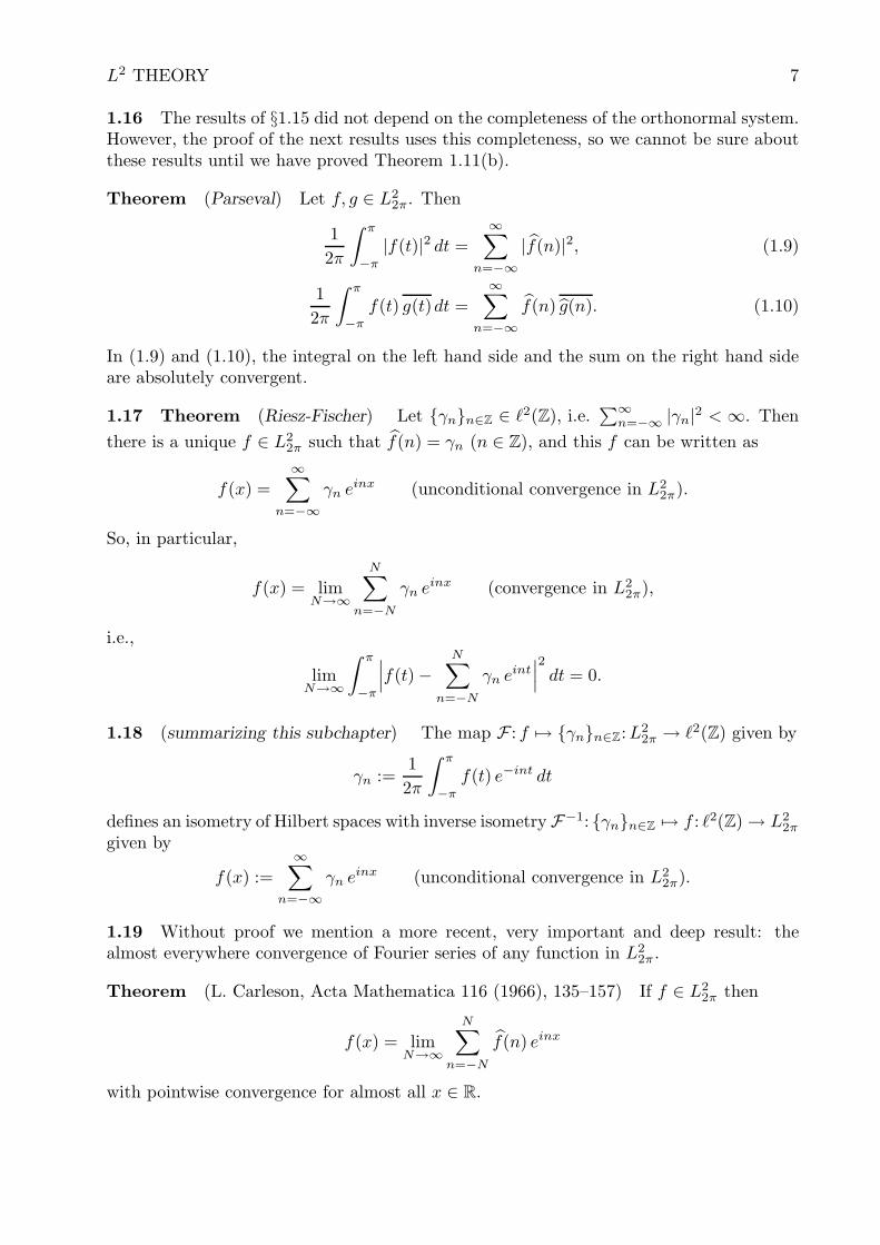
1.16 The results of §1.15 did not depend on the completeness of the orthonormal system.However, the proof of the next results uses this completeness, so we cannot be sure aboutthese results until we have proved Theorem 1.11(b).

Theorem (Parseval) Let f, g ∈ L22π. Then

1

2π

∫ π

−π

|f(t)|2 dt =∞∑

n=−∞

|f(n)|2, (1.9)

1

2π

∫ π

−π

f(t) g(t)dt =

∞∑

n=−∞

f(n) g(n). (1.10)

In (1.9) and (1.10), the integral on the left hand side and the sum on the right hand sideare absolutely convergent.

1.17 Theorem (Riesz-Fischer) Let {γn}n∈Z ∈ ℓ2(Z), i.e.∑∞

n=−∞ |γn|2 < ∞. Then

there is a unique f ∈ L22π such that f(n) = γn (n ∈ Z), and this f can be written as

f(x) =∞∑

n=−∞

γn einx (unconditional convergence in L22π).

So, in particular,

f(x) = limN→∞

N∑

n=−N

γn einx (convergence in L22π),

i.e.,

limN→∞

∫ π

−π

∣∣∣f(t) −N∑

n=−N

γn eint∣∣∣2

dt = 0.

1.18 (summarizing this subchapter) The map F : f 7→ {γn}n∈Z: L22π → ℓ2(Z) given by

γn :=1

2π

∫ π

−π

f(t) e−int dt

defines an isometry of Hilbert spaces with inverse isometry F−1: {γn}n∈Z 7→ f : ℓ2(Z) → L22π

given by

f(x) :=

∞∑

n=−∞

γn einx (unconditional convergence in L22π).

1.19 Without proof we mention a more recent, very important and deep result: thealmost everywhere convergence of Fourier series of any function in L2

2π.

Theorem (L. Carleson, Acta Mathematica 116 (1966), 135–157) If f ∈ L22π then

f(x) = limN→∞

N∑

n=−N

f(n) einx

with pointwise convergence for almost all x ∈ R.

8 CHAPTER 1

1.4 Orthonormal bases with cosines and sines

The orthonormal basis of functions t 7→ eint (n ∈ Z) for L22π (see Theorem 1.11(c))

immediately gives rise to an orthonormal basis for L22π in terms of cosines and sines. We

formulate it in two steps and leave the straightforward proofs to the reader.

1.20 Lemma For n = 1, 2, . . . the two-dimensional subspace of L22π spanned by the

two orthonormal functions t 7→ e±int also has an orthonormal basis given by the twofunctions t 7→

√2 cos(nt) and t 7→

√2 sin(nt).

Proposition The functions t 7→ 1, t 7→√

2 cos(nt) (n = 1, 2, . . .), and t 7→√

2 sin(nt)(n = 1, 2, . . .) form an orthonormal basis for L2

2π.

Note that, in the orthonormal basis of the above Proposition, the cosine functions(including 1) are even and the sine functions are odd. In fact, we can split the Hilbertspace L2

2π as a direct sum of the subspace of even functions and the subspace of oddfunctions, such that the cosines form an orthonormal basis for the first subspace and thesines an orthonormal subspace for the second subspace. Let us first discuss the notion ofdirect sum decomposition.

1.21 Definition Let H be a Hilbert space and let H1 and H2 be closed linear subspacesof H (so H1 and H2 are Hilbert spaces themselves). We say that H is the (orthogonal)direct sum of H1 and H2 (notation H = H1 ⊕ H2) if the two following conditions aresatisfied:(i) The subspaces H1 and H2 are orthogonal to each other.(ii) Each v ∈ H can be written as v = v1 + v2 with v1 ∈ H1 and v2 ∈ H2.

Ex. 1.22 Let H1 and H2 be Hilbert spaces and make H := {(v1, v2) | v1 ∈ H1, v2 ∈ H2}into an inner product space by the rules

(v1, v2) + (w1, w2) := (v1 + w1, v2 + w2), λ(v1, v2) := (λv1, λv2),

〈(v1, v2), (w1, w2)〉 := 〈v1, w1〉 + 〈v2, w2〉.Show that H is a Hilbert space and that it is the direct sum of its two closed linearsubspaces {(v, 0) | v ∈ H1} and {(0, v) | v ∈ H2}.

An example of a direct space decomposition is given by the following Proposition.

1.23 Proposition The space L22π is the orthogonal direct sum of the two closed linear

subspaces

L22π,even := {f ∈ L2

2π | f(t) = f(−t) a.e.},L2

2π,odd := {f ∈ L22π | f(t) = −f(−t) a.e.}.

The maps f 7→ f |[0,π]: L22π,even → L2([0, π]) and f 7→ f |[0,π]: L

22π,odd → L2([0, π]) are

isomorphisms of Hilbert spaces, provided the inner product on L2([0, π]) is normalized as

〈f, g〉 :=1

π

∫ π

0

f(t) g(t)dt. (1.11)

Theorem The functions t 7→ 1 and t 7→√

2 cos(nt) (n = 1, 2, . . .) form an orthonormalbasis of L2

2π,even, and hence also of L2([0, π]) (with inner product (1.11)). The functions

t 7→√

2 sin(nt) (n = 1, 2, . . .) form an orthonormal basis of L22π,odd, and hence also of

L2([0, π]) (with inner product (1.11)).

L2 THEORY 9

Ex. 1.24 Give the proofs of the above Proposition and Theorem.

1.5 Further exercises

Ex. 1.25 Let f be the sawtooth function, i.e. the 2π-periodic function which is given on(0, 2π) by:

f(x) := π − x (0 < x < 2π), (1.12)

and which is arbitarary for x = 0. Show the following:

(a) f ∈ L22π and f(n) = (in)−1 if n 6= 0 and f(0) = 0.

(b)∑∞

n=1 n−2 = π2/6.

Hint Apply formula (1.9).

Ex. 1.26 Show that∞∑

n=1

n−4 = π4/90

by applying formula (1.9) to the function f ∈ L22π such that f(t) := t2 for t ∈ (−π, π).

Ex. 1.27 For 0 6= a ∈ R let fa ∈ L22π such that fa(t) := eat for t ∈ (−π, π).

(a) Compute the Fourier coefficients of fa.(b) Let a, b ∈ R such that a, b, a + b 6= 0. Derive the identity

coth(πa) + coth(πb) =1

π

∞∑

n=−∞

(1

a − in+

1

b + in

)

by applying (1.10) to the functions f := fa and g := fb.(c) Show that the case a = b of this identity yields

coth(πa) = π−1 limN→∞

N∑

n=−N

1

a − in.

Does the right hand side converge? Is it allowed to replace limN→∞

∑Nn=−N by∑∞

n=−∞ ? Conclude that

∞∑

n=1

1

a2 + n2=

π coth(aπ)

4a− 1

4a2(a 6= 0).

This becomes the identity in Exercise 1.25(b) as a → 0.

Ex. 1.28 Put c0(t) := 1, cn(t) :=√

2 cos(nt) (n = 1, 2, . . .), sn(t) :=√

2 sin(nt) (n =1, 2, . . .), and let

〈cm, sn〉 :=1

π

∫ π

0

cm(t) sn(t) dt (m = 0, 1, 2, . . . , n = 1, 2, . . .)

(inner products in L2([0, π])). Consider the ∞ × ∞ matrix with (real) matrix entries〈cm, sn〉, (row indices m and column indices n). Show that the columns of this matrix areorthonormal, and that also the rows are orthonormal, i.e.,

∞∑

m=0

〈cm, sk〉〈cm, sl〉 = δk,l,∞∑

n=1

〈ck, sn〉〈cl, sn〉 = δk,l.

Next compute the matrix entries explicitly.

10 CHAPTER 1

Ex. 1.29 Let f ∈ L22π. For k = 1, 2, . . . put gk(t) := f(kt). Then gk ∈ L2

2π. Express theFourier coefficients of gk in terms of the Fourier coefficients of f .

Ex. 1.30 Let σ, τ ∈ {±1}. Define

L22π,σ,τ := {f ∈ L2

2π | f(−x) = σ f(x) a.e., f(π − x) = τ f(x) a.e.}.

a) Show that the Hilbert space L22π is the direct sum of the four mutually orthogonal

closed linear subspaces L22π,σ,τ (σ, τ ∈ {±1}).

b) For each choice of σ, τ find an orthonormal basis of L22π,σ,τ . (Start with the orthonor-

mal basis for L22π,even or L2

2π,odd given in §1.23.)

c) For each σ, τ give a Hilbert space isomorphism of L22π,σ,τ with L2([0, 1

2π]).

Ex. 1.31 For F a function on R define a function f on (0, 2π) by f(x) := F (cot 12x).

This establishes a one-to-one linear correspondence between functions f on (0, 2π) andfunctions F on R

(a) Show that the map f 7→ F is a Hilbert space isomorphism of L2((0, 2π); (2π)−1 dx)onto L2(R; π−1 (t2 + 1)−1 dt)., i.e.,

1

2π

∫ π

−π

|f(x)|2 dx =1

π

∫ ∞

−∞

|F (t)|2 dt

t2 + 1.

(b) Show that the orthonormal basis of L2((0, 2π); (2π)−1 dx) provided by the functionsx 7→ einx (n ∈ Z), is sent by the map f 7→ F to the orthonormal basis of L2(R; π−1 (t2+1)−1 dt) given by the functions t 7→ ( t+i

t−i)n.

Ex. 1.32 Let V be the linear space of piecewise linear continuous functions on the closedbounded interval [a, b]. So, f ∈ V iff f ∈ C([a, b]) and there is a partition a = a0 < a1 <a2 . . . < an = b such that the restriction of f to [ai−1, ai] is linear for i = 1, . . . , n. LetV0 := {f ∈ V | f(a) = f(b) = 0}. Show that V is dense in C([a, b]) and that V0 is densein Lp([a, b]) (1 ≤ p < ∞).

11

2 L1 theory

2.1 Growth rates of Fourier coefficients

2.1 The Fourier coefficients f(n) (n ∈ Z) of a function f ∈ L12π were defined in formula

(1.8). It follows from this formula that

|f(n)| ≤ ‖f‖1 (f ∈ L12π, n ∈ Z). (2.1)

Hence‖f‖∞ ≤ ‖f‖1 where ‖f‖∞ := sup

n∈Z

|f(n)|.

So f ∈ ℓ∞(Z) if f ∈ L12π. Here ℓ∞(Z) := {(γn)n∈Z | supn∈Z

|γn| < ∞}, a Banach space.

Ex. 2.2 Show that the map f 7→ f : L12π → ℓ∞(Z) is a bounded linear operator. Also

determine its operator norm.

2.3 In §1.15 we gave the so-called Riemann-Lebesgue Lemma in the L2-case. It remainsvalid for the L1-case:

Theorem (Riemann-Lebesgue Lemma) If f ∈ L12π then lim|n|→∞ f(n) = 0.

Proof Let f ∈ L12π. Let ε > 0. We have to look for a natural number N such that

|f(n)| < ε if |n| ≥ N . Since L22π is dense in L1

2π (see §1.10), there exists a function g ∈ L22π

such that ‖f − g‖1 < 12ε. By the Riemann-Lebesgue Lemma for L2 (see §1.15) there exists

N ∈ N such that: |n| ≥ N ⇒ |g(n)| < 12ε. Hence, if |n| ≥ N then

|f(n)| ≤ |f(n) − g(n)| + |g(n)| ≤ ‖f − g‖1 + |g(n)| < 12ε + 1

2ε = ε,

where we used the inequality (2.1).

Ex. 2.4 Define the linear space c0(Z) by

c0(Z) := {{cn}n∈Z ∈ ℓ∞(Z) | lim|n|→∞

cn = 0}.

Show that c0(Z) is a closed linear subspace of ℓ∞(Z). So, in particular, c0(Z) becomes a

Banach space. Note also that f 7→ f : L12π → c0(Z) is a bounded linear map.

2.5 In addition to the space C2π we will deal, for k = 1, 2, . . . or ∞, with the linearspace Ck

2π consisting of 2π-periodic Ck-functions on R. By C02π we will just mean C2π.

Elementary integration by parts yields:

(f ′)(n) = in f(n) (f ∈ C12π, n ∈ Z). (2.2)

This is an important result. Corresponding to the differentiation operator f 7→ f ′ actingon 2π-periodic functions we have on the Fourier transform side the operator multiplyinga function of n by in. Iteration of (2.2) yields:

(f (k))(n) = (in)k f(n) (f ∈ Ck2π, k = 0, 1, 2, . . . , n ∈ Z). (2.3)

For f ∈ C2π the Riemann-Lebesgue Lemma gives that f(n) = o(1) as |n| → ∞, amodest rate of decline for the Fourier coefficients. It turns out that a higher order ofdifferentiability of a 2π-periodic function f implies a faster decline of f(n) as |n| → ∞:

12 CHAPTER 2

Theorem (a) Let k ∈ {0, 1, 2, . . .}. If f ∈ Ck2π then f(n) = o(|n|−k) as |n| → ∞.

(b) If f ∈ C∞2π then f(n) = O(|n|−k) as |n| → ∞ for all k ∈ {0, 1, 2, . . .}.

So we see that for 2π-periodic C∞-functions the Fourier coefficients decrease fasterin absolutele value to zero than any inverse power of |n|. We then say that the Fouriercoefficients are rapidly decreasing.

Proof of Theorem Part (b) follows immediately from part (a). For the proof of part(a) we use equations (2.3) and the Riemann-Lebesgue Lemma:

|f(n)| = |n|−k |(f (k))(n)| = |n|−k o(1) as n → ∞,

since f (k) ∈ C2π if f ∈ Ck2π.

Ex. 2.6 Show that (2.2) still holds if f ∈ C2π with piecewise continuous derivative.

Ex. 2.7 Let f ∈ C2π . Suppose that f can be extended to a function analytic on the openstrip {z ∈ C | |Im z| < K} and continuous on the closed strip {z ∈ C | |Im z| ≤ K}. Show

that |f(n)| = O(e−K|n|) as |n| → ∞.Hint If z ∈ C and |Im z| ≤ K then f(z + 2π) = f(z). Next show by contour integrationthat

f(n) =1

2π

∫ a+π

a−π

f(z) e−inz dz (n ∈ Z, |Im a| ≤ K).

2.8 In the previous sections we derived the behaviour of the Fourier coefficients f(n) fromthe behaviour of the function f . Now we consider the inverse problem: Let coefficients γn

with certain behaviour be given. Find a 2π-periodic function f such that f(n) = γn andgive the behaviour of f .

We say that the doubly infinite sequence (γn)n∈Z is in ℓ1(Z) if‖(γn)‖1 :=

∑∞n=−∞ |γn| < ∞.

Theorem Let (γn) ∈ ℓ1(Z). Put

f(x) :=∞∑

n=−∞

γn einx (x ∈ R), (2.4)

well defined because the series converges absolutely. Then f ∈ C2π and f(n) = γn (n ∈ Z).Also ‖f‖∞ ≤ ‖(γn)‖1.

Proof The absolute convergence of the series on the right hand side of (2.4) is uniformfor x ∈ R because of the Weierstrass test, since |γn einx| ≤ |γn| and

∑∞n=−∞ |γn| < ∞.

The sum of a uniform convergent series of continuous functions is continuous. Since theterms of the series are 2π-periodic in x, the same holds for the sum function. Thus f ∈ C2π.The inequality ‖f‖∞ ≤ ‖(γn)‖1 follows by taking absolute values on both sides of (2.4),and by dominating the absolute value of the sum on the right hand side by the sum of theabsolute values of the terms. Finally, we derive that

f(n) =1

2π

∫ π

−π

(∞∑

m=−∞

γm eimx e−inx

)dx =

∞∑

m=−∞

γm

(1

2π

∫ π

−π

ei(m−n)x dx

)= γn,

where the second equality is permitted because the integral over a bounded interval of auniformly convergent sum of continuous functions equals the sum of the integrals of theterms.

L1 THEORY 13

Ex. 2.9 Let f(x) be given by (2.4). Prove the following statements. Use for (a) and (b)the theorem about differentiation of a series of functions on a bounded interval for whichthe series of derivatives is uniformly convergent.

(a) If∑∞

n=−∞ |n| |γn| < ∞ then f ∈ C12π .

(b) Let k ∈ {0, 1, 2, . . .}. If∑∞

n=−∞ |n|k |γn| < ∞ then f ∈ Ck2π.

(c) Let λ > 1. If γn = O(|n|−λ) as |n| → ∞ then f ∈ Ck2π for all integer k such that

0 ≤ k < λ − 1.

(d) If γn = O(|n|−k) as |n| → ∞ for all k ∈ {0, 1, 2, . . .} then f ∈ C∞2π.

(e) Let K > 0. If γn = O(e−K|n|) as |n| → ∞ then f can be extended to an analyticfunction on the strip {z ∈ C | |Im z| < K}. Compare with Exercise 2.7

2.10 Remark Observe that the Fourier images of L22π and of C∞

2π can be completelycharacterized. Namely, for a given sequence (γn)n∈Z we have:

γn = f(n) (n ∈ Z) for some f ∈ L22π iff

∑∞n=−∞ |γn|2 < ∞;

γn = f(n) (n ∈ Z) for some f ∈ C∞2π iff γn = O(|n|−k) as |n| → ∞ for all k ∈ {0, 1, 2, . . .}.

However, such a characterization is not possible for the Fourier images of C2π, C12π, C2

2π, . . .and of L1

2π.

Ex. 2.11 Let γ0 := 0 and γn := |n|−λ for n ∈ Z\{0}. Then it is known in the literature

for which real values of λ there exists f ∈ L12π such that f(n) = γn (n ∈ Z). For some

values of λ this follows from a non-trivial theorem (see sections 7.17 and 7.19 in van Rooij).However, for some other values of λ the answer is immediate. Give the answer in thesecases.

2.2 Fubini’s Theorem

2.12 For the treatment of convolution we will need Fubini’s Theorem. The Propositionbelow formulates Fubini’s theorem for nonnegative measurable functions, see also syll.Integratietheorie, Sections 5.6–5.8. Next the Theorem below will deal with complex-valuedmeasurable functions. Below we will work with σ-finite measure spaces (X,A, µ) and(Y,B, ν) and their product space (X × Y,A⊗ B, µ × ν), again a σ-finite measure space.

It is helpful to read first the Theorem below for the case that X and Y are boundedintervals, µ and ν are Lebesgue measure, and the function h: X × Y → C is continuous.Then all integrals can also be considered as Riemann integrals and the assumption in theTheorem concerning the absolute convergence of a repeated integral is automatic.

The general Proposition and Theorem below are much more delicate, because measurespaces may be σ-finite rather than finite and because measurable rather than continuousfunctions are considered.

2.13 Proposition Let the function h: X × Y → [0,∞] be measurable with respect tothe σ-algebra A⊗ B. Then:

(a) The function y 7→∫

Xh(x, y) dµ(x) is measurable on B;

(b) The function x 7→∫

Yh(x, y) dν(y) is measurable on A;

14 CHAPTER 2

(c) We have

∫

X×Y

h(x, y) d(µ×ν)(x, y) =

∫

X

(∫

Y

h(x, y) dν(y)

)dµ(x) =

∫

Y

(∫

X

h(x, y) dµ(x)

)dν(y).

(2.5)

Note that all integrals considered in (2.5) are integrals of measurable functions whichtake values on [0,∞]. The integral of such a function is well-defined and it will yield anumber in [0,∞].

Consider next a function h: X × Y → C (so not necessarily non-negative) which ismeasurable with respect to the σ-algebra A ⊗ B. Then the nonnegative function |h| ismeasurable with respect to A⊗B, so the above Proposition will hold with h(x, y) replacedby |h(x, y)|. This we will need in the next theorem.

2.14 Theorem (see Rudin, Theorem 7.8) Let the function h: X ×Y → C be measur-able with respect to the σ-algebra A⊗ B. Suppose that one of the two inequalities belowis valid.

∫

Y

(∫

X

|h(x, y)| dµ(x)

)dν(y) < ∞. (2.6)

∫

X

(∫

Y

|h(x, y)| dν(y)

)dµ(x) < ∞. (2.7)

(So the other inequality is also valid by the above Proposition.) Then:

(a)∫

X|h(x, y)| dµ(x) < ∞ for y outside some set Y0 ⊂ Y of ν-measure 0 and the function

y 7→∫

Xh(x, y) dµ(x): Y \Y0 → C, arbitrarily extended to a complex-valued function

on Y , is ν-integrable on Y .

(b)∫

Y|h(x, y)| dν(y) < ∞ for x outside some set X0 ⊂ X of µ-measure 0 and the function

x 7→∫

Yh(x, y) dν(y): X\X0 → C, arbitrarily extended to a complex-valued function

on X , is µ-integrable on X .

(c) Formula (2.5) is valid.

The crucial condition to be checked in this Theorem is inequality (2.6) or (2.7). Theimportant conclusion in the Theorem is that (almost) all integrals in (2.5) are well-definedand that the equalities in (2.5) (in particular the second one) hold.

2.3 Convolution

2.15 Definition The convolution product of two 2π-periodic functions f, g is a functionf ∗ g on R given by

(f ∗ g)(x) :=1

2π

∫ π

−π

f(t) g(x− t) dt (x ∈ R), (2.8)

provided the right hand side is well-defined. Then, clearly, f ∗ g is also 2π-periodic andf ∗ g = g ∗ f . Check these two properties by simple transformations of the integrationvariable in (2.8)

For deriving further properties of the convolution product, the easiest case is whenf, g are continuous:

L1 THEORY 15

2.16 Proposition If f, g ∈ C2π then f ∗ g ∈ C2π and

(f ∗ g)(n) = f(n) g(n) (n ∈ Z). (2.9)

Proof For the proof of the continuity (in fact uniform continuity) of f ∗ g observe that∣∣∣∣

1

2π

∫ π

−π

f(t) (g(x− t) − g(y − t)) dt

∣∣∣∣ ≤ ‖f‖1 supt∈R

|g(x − t) − g(y − t)|.

Let ε > 0. Since any periodic continuous function is uniformly continuous on R (why?),there exists δ > 0 such that |g(x − t) − g(y − t)| < ε for all t ∈ R if |x − y| < δ. Hence|(f ∗ g)(x)− (f ∗ g)(y)| < ε ‖f‖1 if |x − y| < δ.

For the proof of (2.9) use Fubini’s theorem in the case of continuous functions on abounded interval. Thus

(f ∗ g)(n) =1

4π2

∫ π

−π

(∫ π

−π

f(t) g(x− t) dt

)e−inx dx

=1

4π2

∫ π

−π

f(t) e−int

(∫ π

−π

g(x − t) e−in(x−t) dx

)dt

=1

4π2

∫ π

−π

f(t) e−int g(n) dt = f(n) g(n).

Ex. 2.17 Let f(x) := eimx, g(x) := einx (m, n ∈ Z). Compute f ∗ g. Also check that theresult agrees with equality (2.9).

Ex. 2.18 Prove by Fubini’s theorem in the case of continuous functions on a boundedinterval the following. If f, g, h ∈ C2π then

(f ∗ g) ∗ h = f ∗ (g ∗ h) (associativity). (2.10)

2.19 Definition-Theorem Let f, g ∈ L12π. Let (f ∗ g)(x) be defined by (2.8) for those

x ∈ R for which the integral on the right hand side of (2.8) converges absolutely.

(a) For almost all x ∈ R the integral on the right hand side of (2.8) converges absolutely.Extend f ∗g to a (2π-periodic) function on R by choosing arbitrary values of (f ∗g)(x)on the set of measure zero where f(x) is not yet defined by (2.8). Then f ∗ g ∈ L1

2π

and‖f ∗ g‖1 ≤ ‖f‖1 ‖g‖1. (2.11)

(b) The equivalence class of f ∗ g only depends on the equivalence classes of f and g. Inother words, for f, g ∈ L1

2π the convolution product f ∗ g is well-defined as an elementof L1

2π.

(c) For f, g ∈ L12π, formula (2.9) is valid.

(d) For f, g, h ∈ L12π, the associativity property (2.10) is valid.

Proof Let f, g ∈ L12π. First observe that

1

4π2

∫ π

−π

(∫ π

−π

|f(t) g(x− t)| dx

)dt =

1

4π2

∫ π

−π

|f(t)|(∫ π

−π

|g(x − t)| dx

)dt

=1

2π

∫ π

−π

|f(t)| ‖g‖1 dt = ‖f‖1 ‖g‖1 < ∞. (2.12)

16 CHAPTER 2

Hence, by Fubini’s Theorem 2.14 we have that

∫ π

−π

|f(t) g(x− t)| dt < ∞

for almost all x. Thus, (f ∗ g)(x) is well-defined by (2.8) for almost all x, and f ∗ g ismeasurable on R. Again by Theorem 2.14, it follows that

1

4π2

∫ π

−π

∣∣∣∣∫ π

−π

f(t) g(x− t) dt

∣∣∣∣ dx < ∞.

So f ∗ g ∈ L12π. For the proof of (2.11) use that

‖f ∗ g‖1 ≤ 1

4π2

∫ π

−π

(∫ π

−π

|f(t) g(x− t)| dt

)dx =

1

4π2

∫ π

−π

(∫ π

−π

|f(t) g(x− t)| dx

)dt

by Proposition 2.13, and combine with (2.12).For the proof of part (b) let f, g ∈ L1

2π with ‖f‖1 = 0 or ‖g‖1 = 0. Then ‖f ∗ g‖1 = 0because of (2.11).

For the proof of (c) repeat the proof of (2.9) for the continuous case. We can nowjustify the interchange of integration order in the second equality of that proof by Fubini’sTheorem 2.14, because

1

4π2

∫ π

−π

(∫ π

−π

|f(t) g(x− t) e−inx| dx

)dt < ∞.

This last inequality is true because the left hand side equals ‖ |f | ∗ |g| ‖1 < ∞.Finally (d) can be proved similarly as in Exercise 2.18, with justification of the inter-

change of integration order by Theorem 2.14.

2.20 Proposition If f ∈ L12π and g ∈ C2π then f ∗ g ∈ C2π and

‖f ∗ g‖∞ ≤ ‖f‖1 ‖g‖∞. (2.13)

Proof The proof given in Proposition 2.16 that f ∗g ∈ C2π if f, g ∈ C2π , still works if theassumption on f is relaxed to f ∈ L1

2π. The proof of inequality (2.13) is straightforward.

Ex. 2.21 Show: If f, g ∈ L22π then f ∗ g ∈ C2π and

‖f ∗ g‖∞ ≤ ‖f‖2 ‖g‖2. (2.14)

Hint First show that supx∈R|(f ∗g)(x)| ≤ ‖f‖2 ‖g‖2 if f, g ∈ L2

2π. Next use this inequalityand the fact that f ∗ g is continuous if f, g ∈ C2π (see Proposition 2.16), together with thedensity of C2π in L2

2π and the completeness of the Banach space C2π with respect to thesup norm.

L1 THEORY 17

2.4 Further exercises

Ex. 2.22 Show that

∞∑

n=0

2−n cos(nx) =4 − 2 cosx

5 − 4 cosx(x ∈ R).

Compare with Exercise 2.9(e).

Ex. 2.23 Let A ∈ C such that |A| 6= 1. Let f(x) := (A + eix)−1 (x ∈ R). Compute the

Fourier coefficients f(n).

Ex. 2.24 Let f ∈ L12π. Express g(n) in terms of the f(m) if:

(a) g(x) = f(x + a) (a ∈ R);

(b) g(x) = f(−x);

(c) g(x) = f(x);

(d) g(x) = f(−x).

Ex. 2.25 Let f ∈ L12π, g ∈ C1

2π. Show that f ∗ g ∈ C12π and that (f ∗ g)′ = f ∗ g′.

18

3 The Dirichlet kernel

3.1 Definition of the Dirichlet kernel

3.1 Let f ∈ L12π. The formal doubly infinite series

∑

n∈Z

f(n)einx (3.1)

is called the Fourier series of f . We will see that this series converges in a certain sense tof(x), but the type of convergence will depend on the nature of f . Saying that the series(3.1) converges in some sense to f(x) amounts to the same as saying that the sequence ofpartial Fourier sums

SN (x) = (SN [f ])(x) :=

N∑

n=−N

f(n) einx (N = 0, 1, 2, . . . , x ∈ R) (3.2)

converges in some sense to f(x) as N → ∞. Therefore it is important to examine thefunctions SN [f ] in more detail.

3.2 Definition-Proposition The partial Fourier sum (3.2) can be written as

(SN [f ])(x) = (f ∗ DN )(x) =1

2π

∫ π

−π

f(t) DN (x − t) dt =1

2π

∫ π

−π

f(x + t) DN (t) dt, (3.3)

where DN is the Dirichlet kernel:

DN (x) :=

N∑

n=−N

einx =

sin((N + 12 )x)

sin( 12x)

(x /∈ 2πZ),

2N + 1 (x ∈ 2πZ).

(3.4)

The Dirichlet Kernels D2, D5, D10, centered at 0, 2π, 4π respectively.

(See also the graph of DN in van Rooij, p.13.)

DIRICHLET KERNEL 19

Proof Observe from (3.2) that

(SN [f ])(x) =1

2π

∫ π

−π

f(t)

(N∑

n=−N

ein(x−t)

)dt.

From (3.4) we see that DN ∈ C2π and that it is an even function. The third equality in(3.3) uses these last facts.

3.2 Criterium for convergence of Fourier series in one point

3.3 We will need the following three easy consequences of (3.4):

1

2π

∫ π

−π

DN (t) dt = 1, (3.5)

|DN (x)| ≤ 1

| sin( 12x)| ≤

π

|x| (0 < |x| ≤ π), (3.6)

and

DN (x) =e

12 ix

2i sin( 12x)

eiNx − e−12 ix

2i sin( 12x)

e−iNx (x /∈ 2πZ). (3.7)

3.4 Theorem Let f ∈ L12π, a ∈ R. Suppose that one of the two following conditions

holds:

(a) There are M, α, δ > 0 such that

|f(a + t) − f(a)| ≤ M |t|α for −δ < t < δ. (3.8)

(b) f is continuous in a and also right and left differentiable in a.

Then we have:lim

N→∞(SN [f ])(a) = f(a).

Remark Condition (a) of Theorem 3.4 implies continuity of f in a. Functions f satisfyingcondition (a) are said to be Holder continuous of order α in a. (The terminology Lipschitz

continuous of order α is equally common.) If (b) holds then |f(a+t)−f(a)||t| is bounded for t

in some neighbourhood of 0 since it has a limit as t ↓ 0 and as t ↑ 0. Thus if (b) holds then(a) is satisfied with α = 1. So, we only need to prove the Theorem under condition (a).

Proof of Theorem 3.4 Assume condition (a). Let ε > 0. We want to show that|SN (a) − f(a)| < ε for N sufficiently large. It follows from (3.3), (3.5) and (3.7) that

SN (a) − f(a) =1

2π

∫ π

−π

(f(a + t) − f(a)) DN(t) dt

=

∫ π

−π

ga,+(t)eiNt dt −∫ π

−π

ga,−(t)e−iNt dt, (3.9)

where

ga,±(t) =1

2π

e±12 it

2i sin( 12 t)

(f(a + t) − f(a)) (0 < |t| < π). (3.10)

For 0 < |t| < δ we can estimate |ga,±(t)| < 14M |t|α−1 (use (3.6) and (3.8)). For δ < |t| < π

we can estimate |ga,±(t)| < (4π sin( 12δ))−1|f(a+ t)−f(a)|. Hence the functions ga,± are in

L1([−π, π]). By the Riemann-Lebesgue Lemma (Theorem 2.3) it follows that (3.9) tendsto 0 as N → ∞.

20 CHAPTER 3

3.5 Theorem Let f ∈ L12π, let a ∈ R, and suppose that the limits

f(a+) := limx↓a

f(x), f(a−) := limx↑a

f(x)

exist. Suppose that one of the two following conditions holds:

(a) There are M, α, δ > 0 such that

|f(a + t) − f(a+)| ≤ Mtα and |f(a − t) − f(a−)| ≤ Mtα for 0 < t < δ.

(b) f is right and left differentiable in a in the sense that the following two limits exist:

f ′(a+) := limt↓0

f(a + t) − f(a+)

t, f ′(a−) := lim

t↓0

f(a − t) − f(a−)

−t.

Then we have:lim

N→∞(SN [f ])(a) = 1

2(f(a+) + f(a−)).

Proof Since DN is an even function, we conclude from (3.3) that

SN (a) =1

2π

∫ π

−π

12(f(a + t) + f(a − t)) DN (t) dt.

Hence

SN (a) − 12 (f(a+) + f(a−)) =

1

2π

∫ π

−π

(f(a + t) + f(a − t)

2− f(a+) + f(a−)

2

)DN (t) dt.

Now put g(t) := 12 (f(a + t) + f(a − t)) for 0 < |t| ≤ π and g(0) := limt→0 g(t) =

12 (f(a+)+f(a−)). Then condition (a) or (b) for f at the point a implies the corresponding

condition in Theorem 3.4 for g at the point 0. Now apply Theorem 3.4 to g at 0.

3.6 Corollary (localization principle) Let f, g ∈ L12π, let a ∈ R, and suppose that

f(x) = g(x) for x in a certain neighbourhood of a. Then precisely one of the following twoalternatives holds for the two sequences

((SN [f ])(a)

)∞N=0

and((SN [g])(a)

)∞N=0

:

(a) The two sequences both converge and have the same limit.

(b) The two sequences both diverge.

Proof Apply Theorem 3.4 to the function f − g at a. Since f − g is identically zero in aneighbourhood of a, we conclude that limN→∞(SN [f − g])(a) = 0. Hence

limN→∞

((SN [f ])(a)− (SN [g])(a)

)= 0.

Thus the convergence and possible sum of the Fourier series of a function f ∈ L12π at

a point a is completely determined by the restriction of f to an arbitrarily small neigh-bourhood of f . If we leave a given function f unchanged on such a neighbourhood, butchange it elsewhere, then the Fourier coefficients f(n) may become completely different,but convergence or divergence and the possible sum of the Fourier series at a will remainthe same. This explains why the above Corollary is called localization principle.

DIRICHLET KERNEL 21

Ex. 3.7 Let f be the sawtooth function defined in Exercise 1.25, formula (1.12). Putf(x) := 0 for x ∈ 2πZ.(a) Prove that

f(x) = limN→∞

(SN [f ])(x) = 2

∞∑

n=1

sin(nx)

n(3.11)

with pointwise convergence for all x ∈ R.(b) Show by substitution of x := π/2 or x := π/4 in (1.12), (3.11) that

π

4= 1 − 1

3+

1

5− 1

7+ · · · , (3.12)

π√8

= 1 +1

3− 1

5− 1

7+

1

9+

1

11− 1

13− . . . . (3.13)

Ex. 3.8 Let 0 < δ < π. Let f be a 2π-periodic function which is given on [−π, π] by:

f(x) :=

{1 if x ∈ [−δ, δ],0 if δ < |x| ≤ π.

(a) Determine f(n) (n ∈ Z).(b) Determine

δ

π+ lim

N→∞

∑

0<|n|≤N

sin(nδ)

πneinx

provided the limit exists.

Ex. 3.9 Let f be a 2π-periodic function which is C1 outside 2πZ and such that f(0+),

f(0−), f ′(0+), f ′(0−) exist in the sense of Theorem 3.5. Prove that f(n) = O(|n|−1) as

|n| → ∞, but not necessarily f(n) = o(|n|−1) as |n| → ∞.Hint Use Theorem 2.5 and Exercise 1.25(a).

Ex. 3.10 Let f be a 2π-periodic function which is C1 outside a discrete set X having theproperty that X ∩ [−π, π) is a finite set. Assume that f(x+), f(x−), f ′(x+), f ′(x−) exist

in the sense of Theorem 3.5 for each x ∈ X . Prove that f(n) = O(|n|−1) as |n| → ∞.

3.3 Continuous functions with non-convergent Fourier series

We will now show in a “soft” way (i.e., by using functional analytic methods) that thereexists a 2π-periodic continuous function for which the Fourier series does not convergeeverywhere. For this we need a “hard” estimate of the Dirichlet kernel in the two lemmasbelow. This estimate will also be useful elsewhere. We refer to Stein & Shakarchi foran explicit example of a 2π-periodic continuous function with not everywhere convergingFourier series.

3.11 Lemma Let

θ(x) := cot( 12x) − 2x−1 (0 < |x| < 2π). (3.14)

22 CHAPTER 3

Then

DN (x) =2 sin(Nx)

x+ θ(x) sin(Nx) + cos(Nx) (0 < |x| < 2π). (3.15)

Proof It follows from (3.4) that, for 0 < |x| < 2π,

DN (x) =sin((N + 1

2 )x)

sin( 12x)

= sin(Nx) cot( 12x) + cos(Nx).

Ex. 3.12 Show the following:(a) limx→0 θ(x) = 0;(b) limx→0 θ′(x) = −1

6 ;(c) Put θ(x) := 0. Then θ is differentiable and strictly decreasing on (−2π, 2π).(d) θ(π) = −2π−1, θ(−π) = 2π−1, sup−π≤x≤π |θ(x)| = 2π−1.

3.13 Lemma We have∫ π

−π

|DN (x)| dx = 8π−1 log N + O(1) as N → ∞.

In particular,

limN→∞

∫ π

−π

|DN (x)| dx = ∞.

Proof It follows from (3.15) and Exercise 3.12(d) that∣∣|DN (x)| − |2x−1 sin(Nx)|

∣∣ ≤ |DN (x) − 2x−1 sin(Nx)| ≤ 2π−1 + 1 (0 < |x| < π).

Hence ∫ π

−π

|DN (x)| dx = 2

∫ π

−π

∣∣∣∣sin(Nx)

x

∣∣∣∣ dx + O(1) as N → ∞.

Next we write

2

∫ π

−π

∣∣∣∣sin(Nx)

x

∣∣∣∣ dx = 4

∫ N

0

| sin(πx)|x

dx

= 4N−1∑

n=0

∫ 1

0

sin(πx)

x + ndx

= 4N−1∑

n=1

∫ 1

0

sin(πx)

x + ndx + O(1) as N → ∞

(1)= 4π−1

N−1∑

n=1

(n−1 + (n − 1)−1) − 4π−1N∑

n=1

∫ 1

0

cos(πx)

(x + n)2dx + O(1) as N → ∞

(2)= 8π−1

N∑

n=1

n−1 + O(1) as N → ∞

(3)= 8π−1 log N + O(1) as N → ∞.

In equality (1) we used integration by parts. In equality (2) we majorized |∫ 1

0(x +

n)−2 cos(πx) dx| by n−2 and we used that∑N

n=1 n−2 = O(1) as N → ∞. In equality

(3) we used that∑N

n=1 n−1 = log N + O(1) as N → ∞ (by comparing with the corre-sponding Riemann integral, see the definition of Euler’s constant γ).

DIRICHLET KERNEL 23

Ex. 3.14 Let φ: [−π, π] → R be continuous with only finitely many zeros. Define thelinear functional L: C2π → C by

L(f) :=1

2π

∫ π

−π

f(x) φ(x) dx (f ∈ C2π). (3.16)

Prove that L is a bounded linear functional with operator norm

‖L‖ = ‖φ‖1 =1

2π

∫ π

−π

|φ(x)| dx. (3.17)

3.15 Theorem For all x ∈ R there exists f ∈ C2π such that the sequence((SN [f ])(x)

)∞N=0

does not converge to a finite limit.

Proof Without loss of generality we may take x := 0. Define the linear functionalLN : C2π → C by

LN (f) := (SN [f ])(0) =1

2π

∫ π

−π

f(t) DN (t) dt.

It follows from Exercise 3.14 that ‖LN‖ = ‖DN‖1, and it follows next from Lemma 3.13that the sequence (‖LN‖)∞N=0 is unbounded. Now suppose that limN→∞ LN (f) exists forall f ∈ C2π . Then, for all f ∈ C2π , the sequence (LN (f))∞N=0 is bounded. Hence, bythe Banach-Steinhaus theorem (see syll. Functionaalanalyse), the sequence (‖LN‖)∞N=0 isbounded. This is a contradiction.

Ex. 3.16 Let f ∈ L12π and let a ∈ R. Prove that for the two sequences

((SN [f ])(a)

)∞N=0

and

1

π

∫ π

−π

f(a + t)sin(Nt)

tdt, N = 0, 1, 2, . . .

precisely one of the following two alternatives holds:

(a) Both sequences converge with the same limit.

(b) Both sequences diverge.

Conclude that, for f satisfying one of the conditions of Theorem 3.5, we have

12 (f(a+) + f(a−)) = π−1 lim

N→∞

∫ π

−π

f(a + t)sin(Nt)

tdt. (3.18)

Ex. 3.17 Prove, by using (3.18), that

∫ ∞

0

sin x

xdx = lim

N→∞

∫ π

0

sin(Nt)

tdt = 1

2π. (3.19)

24 CHAPTER 3

3.4 Injectivity of the Fourier transform

3.18 In this subsection we will prove that a function f ∈ L12π which has all its Fourier

coefficients f(n) = 0, is almost everywhere equal to zero. For the case that f ∈ L22π, this

was already implied by Parseval’s identity (1.9). However, Parseval’s identity dependedon Theorem 1.11, for which we postponed the proof. Let us first consider the case thatf ∈ C2π .

Proposition Let f ∈ C2π such that f(n) = 0 for all n ∈ Z. Then f = 0.

Proof Let F (x) :=∫ x

0f(t) dt. Then F is a C1-function on R and, because f(0) = 0,

the function F is 2π-periodic. Thus F ∈ C12π . Since F ′ = f , we have f(n) = in F (n) (see

(2.2)). Hence F (n) = 0 if n 6= 0. It follows that (SN [F ])(x) = F (0). By Theorem 3.4 we

conclude that F (x) = limN→∞(SN [F ])(x) = F (0). Hence f(x) = F ′(x) = 0.For the similar result in the case that f ∈ L1

2π we proceed as follows.

3.19 Lemma Let f ∈ L12π such that f(0) = 0. Put F (x) :=

∫ x

0f(t) dt. Then F ∈ C2π

and f(n) = in F (n).

Proof Continuity of F is a consequence of the dominated convergence theorem, appliedto the functions fχx,t, where χx,t is the characteristic function of the interval [x, x + t)and letting t → 0. Now we compute for n 6= 0:

F (n) =

∫ 2π

0

∫ x

0

f(t)e−inxdt dx =

∫ 2π

0

∫ 2π

t

e−inxdxf(t) dt

=

∫ 2π

0

(e−int − 1

in

)f(t) dt =

1

in(f(n) − f(0)) =

1

inf(n).

We used Fubini’s theorem for the second equality.Remark It is a non trivial result of Lebesgue that for almost all x F ′(x) exists and

equals f(x). (see Rudin, Theorem 8.17)

3.20 Theorem (a) Let f ∈ L12π such that f(n) = 0 for all n ∈ Z. Then f = 0 a.e. .

(b) Let f, g ∈ L12π such that f(n) = g(n) for all n ∈ Z. Then f = g a.e. .

Proof It is sufficient to prove part (a). Let F be as in Lemma 3.19. Then it follows

that F ∈ C2π and that F (n) = 0 for n 6= 0. Thus F − F (0) = 0 by Proposition 3.18.

Since F (0) = 0, we conclude that F = 0. It follows that∫ b

af(t) dt = 0 for every choice of

a, b ∈ R. But then∫

Ef(t) dt = 0 for (bounded) open and also for (bounded) closed sets.

By regularity of Lebesgue measure, we conclude that∫

Ef dt = 0 for every Borel set. It

follows that f = 0 a.e. .

3.21 Corollary (a) The linear span of the functions t 7→ eint (n ∈ Z) is dense in L22π

with respect to the norm ‖ . ‖2.

(b) The functions t 7→ eint (n ∈ Z) form an orthonormal basis of L22π.

Proof Apply Definition-Theorem 1.12 to the case f ∈ L22π of Theorem 3.20.

DIRICHLET KERNEL 25

So we have now proved parts (b) and (c) of Theorem 1.11, therefore we have alsodefinitely established all results in subchapter 1.2 which depended on Theorem 1.11, seethe summarizing §1.18. In the next chapter we will also prove part (a) of Theorem 1.11.

As a corollary of the injectivity result of Theorem 3.20 we can also give the followingaddition to Theorem 2.8.

3.22 Corollary Let f ∈ L12π. If f ∈ ℓ1(Z) then f ∈ C2π and, for almost all x ∈ R:

f(x) =

∞∑

n=−∞

f(n) einx. (3.20)

The right hand side of (3.20) converges absolutely and uniformly for x ∈ R.

Proof Denote the right hand side of (3.20) by g(x). Then, by 2.8, g ∈ C2π and g(n) =

f(n) for all n ∈ Z. Now apply Theorem 3.20(b).

3.5 Uniform convergence of Fourier series

We will now consider an analogue of Theorem 3.4 such that f satisfies not just a Holdercondition at one point, but a uniform Holder condition on some interval (a, b). Then itwill turn out that SN [f ] converges uniformly to f on each compact subset of (a, b). Forf ∈ C2

2π this result is almost immediate:

3.23 Proposition Let f ∈ C22π. Then limN→∞ SN [f ] = f , uniformly on R.

Proof It follows from Theorem 2.5(a) that f(n) = o(|n|−2) as |n| → ∞. Now applyCorollary 3.22.

3.24 The following lemma quickly follows from the well-known Arzela-Ascoli theorem(see for instance A. Browder, Mathematical Analysis, Springer, 1996, Theorem 6.71 andCorollary 6.73).

Lemma Let (X, d) be a compact metric set. Let (φn)∞n=1 be a sequence of complex-valued functions on X which is equicontinuous on X , i.e., such that, for each ε > 0, thereis a δ > 0 with the property that |φn(x) − φn(y)| < ε for al n ∈ N if x, y ∈ X andd(x, y) < δ. Suppose that limn→∞ φn(x) = 0 for x ∈ X . Then limn→∞ φn = 0 uniformlyon X .

Proof Suppose that the convergence φn → 0 is not uniform on X . Then there exist ε > 0,an increasing sequence of positive integers n1, n2, . . ., and a sequence x1, x2, . . . in X suchthat |φnk

(xk)| ≥ ε. By compactness of X the sequence x1, x2, . . . has a subsequenceconverging to some x0 ∈ X . Without loss of generality we may assume that the sequencex1, x2, . . . already converges to x0. Then

|φnk(xk)| ≤ |φnk

(xk) − φnk(x0)| + |φnk

(x0)|.

By the assumptions, there exists K ∈ N such that |φnk(x0)| < 1

2ε if k ≥ K and |φm(xk)−

φm(x0)| < 12ε for all m ∈ N if k ≥ K. Hence φnk

(xk) < ε if k ≥ K. This is a contradiction.

26 CHAPTER 3

3.25 Theorem Let f ∈ L12π. Suppose that there exist an interval (a, b) and positive

real numbers M, α such that

|f(x) − f(y)| ≤ M |x − y|α for all x, y ∈ (a, b) (3.21)

(a uniform Holder condition on (a, b)). Then limN→∞ SN [f ] = f uniformly on each subin-terval [c, d] with a < c < d < b.

Proof By the proof of Theorem 3.4 we can write

SN (x) − f(x) =

∫ π

−π

gx,+(t)eiNt dt −∫ π

−π

gx,−(t)e−iNt dt (3.22)

with the functions gx,± being given by (3.10). Put

φN,±(x) :=

∫ π

−π

gx,±(t) e±iNt dt (x ∈ [c, d]).

By (3.21) and the proof of Theorem 3.4, the functions gx,± belong to L12π for x ∈ [c, d]. So

limN→∞ φN,±(x) = 0 for x ∈ [c, d] by the Riemann-Lebesgue Lemma (Theorem 2.3). Wewill show that the functions φN,± are equicontinuous on [c, d]. Then we can apply Lemma3.24 and thus prove the Theorem.

Let 0 < δ < π such that δ < c − a and δ < b − d. Then we can estimate for x ∈ [c, d]and 0 < |t| < δ that |gx,±(t)| < 1

4M |t|α−1 (use (3.21) and (3.6)). We can estimate for

x, y ∈ [c, d] and δ < |t| < π that

|gx,±(t) − gy,±(t)| < (4π sin( 12δ))−1

(|f(x + t) − f(y + t)| + |f(x) − f(y)|

).

Next, for x, y ∈ [c, d]:

|φN,±(x) − φN,±(y)| ≤(∫

|t|<δ

+

∫

δ<|t|<π

)|gx,±(t) − gy,±(t)| dt

≤ M

∫ δ

0

|t|α−1 dt +1

4π sin( 12δ)

∫ π

−π

|f(x + t) − f(y + t)| dt +|f(x) − f(y)|

2 sin( 12δ)

.

Let ε > 0. We will find γ > 0 such that the last expression is dominated by ε if x, y ∈ [c, d]

and |x− y| < γ. First take δ such that M∫ δ

0|t|α−1 dt < ε/3. Then we can find γ > 0 such

that the second and third term are dominated by ε/3 if |x − y| < γ. For the third termthis follows because f is uniformly continuous on [c, d]. For the second term this followsfrom Proposition 1.9. This settles the equicontinuity of the functions φN,± on [c, d]. Thuswe can apply Lemma 3.24 and the Theorem will follow.

3.26 Corollary Let f ∈ C12π, or let f ∈ C2π with piecewise continuous derivative. Then

limN→∞ SN [f ] = f , uniformly on R.

Ex. 3.27 Let the 2π-periodic function f be determined by f(x) := |x| for −π ≤ x ≤ π.

Determine the Fourier coefficients f(n). The uniform convergence of (SN [f ])∞N=0 on R isimplied by Corollary 3.26. Check this uniform convergence independently by using theexplicit values of f(n).

DIRICHLET KERNEL 27

3.6 The Gibbs phenomenon

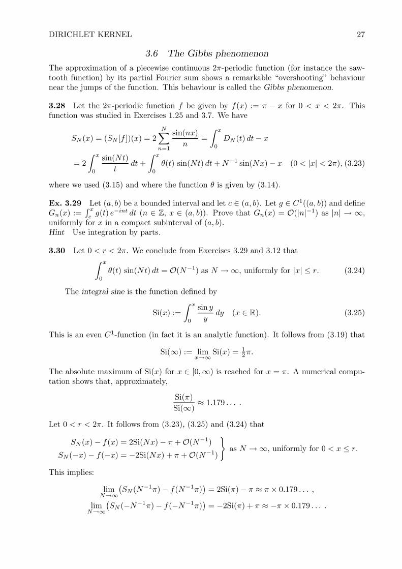
The approximation of a piecewise continuous 2π-periodic function (for instance the saw-tooth function) by its partial Fourier sum shows a remarkable “overshooting” behaviournear the jumps of the function. This behaviour is called the Gibbs phenomenon.

3.28 Let the 2π-periodic function f be given by f(x) := π − x for 0 < x < 2π. Thisfunction was studied in Exercises 1.25 and 3.7. We have

SN (x) = (SN [f ])(x) = 2N∑

n=1

sin(nx)

n=

∫ x

0

DN (t) dt − x

= 2

∫ x

0

sin(Nt)

tdt +

∫ x

0

θ(t) sin(Nt) dt + N−1 sin(Nx) − x (0 < |x| < 2π), (3.23)

where we used (3.15) and where the function θ is given by (3.14).

Ex. 3.29 Let (a, b) be a bounded interval and let c ∈ (a, b). Let g ∈ C1((a, b)) and defineGn(x) :=

∫ x

cg(t) e−int dt (n ∈ Z, x ∈ (a, b)). Prove that Gn(x) = O(|n|−1) as |n| → ∞,

uniformly for x in a compact subinterval of (a, b).Hint Use integration by parts.

3.30 Let 0 < r < 2π. We conclude from Exercises 3.29 and 3.12 that∫ x

0

θ(t) sin(Nt) dt = O(N−1) as N → ∞, uniformly for |x| ≤ r. (3.24)

The integral sine is the function defined by

Si(x) :=

∫ x

0

sin y

ydy (x ∈ R). (3.25)

This is an even C1-function (in fact it is an analytic function). It follows from (3.19) that

Si(∞) := limx→∞

Si(x) = 12π.

The absolute maximum of Si(x) for x ∈ [0,∞) is reached for x = π. A numerical compu-tation shows that, approximately,

Si(π)

Si(∞)≈ 1.179 . . . .

Let 0 < r < 2π. It follows from (3.23), (3.25) and (3.24) that

SN (x) − f(x) = 2Si(Nx) − π + O(N−1)

SN (−x) − f(−x) = −2Si(Nx) + π + O(N−1)

}as N → ∞, uniformly for 0 < x ≤ r.

This implies:

limN→∞

(SN (N−1π) − f(N−1π)

)= 2Si(π) − π ≈ π × 0.179 . . . ,

limN→∞

(SN (−N−1π) − f(−N−1π)

)= −2Si(π) + π ≈ −π × 0.179 . . . .

28 CHAPTER 3

Also, for 0 < δ < π, we have

limN→∞

(sup

0<x≤δ(SN (x) − f(x))

)= 2Si(π) − π, (3.26)

limN→∞

(inf

−δ≤x<0(SN (x) − f(x))

)= −2Si(π) + π, (3.27)

but

limN→∞

(sup

δ≤x≤2π−δ|SN (x) − f(x)|

)= 0

by Theorem 3.25.

Ex. 3.31 Let h ∈ C1([0, 2π]) Let g be a 2π-periodic function which coincides with hon (0, 2π). Write g(0+) := h(0) and g(0−) := h(2π). Assume that g(0+) ≥ g(0−). Let0 < δ < π. Prove that

limN→∞

(sup

0<x≤δ((SN [g])(x)− g(x))

)= 1

2 (g(0+) − g(0−)) (2π−1Si(π) − 1),

limN→∞

(inf

−δ≤x<0((SN [g])(x)− g(x))

)= −1

2 (g(0+) − g(0−)) (2π−1Si(π) − 1).

Hint Let the 2π-periodic function f be given by f(x) := π − x for 0 < x < 2π. Put

p(x) := g(x) − g(0+) − g(0−)

2πf(x) (0 < x < 2π).

Then p ∈ C2π with piecewise continuous derivative. Now use (3.26), (3.27), and Corollary3.26.

The Gibbs phenomenon.

Left: the sawtooth and S64, Right: (SN (N−1x) − f(N−1x))/π for N = 1024

DIRICHLET KERNEL 29

3.7 Further exercises

Ex. 3.32 Prove that

sin x + 13 sin 3x + 1

5 sin 5x + · · · = π/4 if 0 < x < π.

Hint Use Exercise 3.8 or use (1.12), (3.11).

Ex. 3.33 Let φ ∈ L12π. Define the linear functional L: C2π → C by (3.16). Prove that L

is a bounded linear functional with norm given by (3.17).Hint Use Exercises 3.14 and 1.32.

Ex. 3.34 Prove that DN (x) can be written as a polynomial of degree 2N in cos( 12x).

Ex. 3.35 Prove that between each two successive zeros of DN (x) there is precisely onezero of D′

N (x).

Ex. 3.36 1) Let {an}∞1 , {an}∞1 be sequences of complex numbers. Prove (for N =1, 2, . . .) the Summation by parts formula

N∑

n=1

an(bn+1 − bn) = aN+1bN+1 − a1b1 −N∑

n=1

bn+1(an+1 − an).

2) Write down a version of this formula for the case where bn =∑n

j=1 cj .

3) Give a direct proof of the convergence of the series in exercise 3.32 (without usingthat this is a Fourier series of a smooth function)

4) Show that the series∞∑

n=2

sinnx

log n

converges pointwise for every x.

5) What can you say about uniform convergence?

30

4 The Fejer kernel

4.1 Cesaro convergence

4.1 Definition Let (an)∞n=1 be a sequence of complex numbers. If the sequence doesnot have a limit then we may try to find a limit in a generalized sense by considering anew sequence (bn)∞n=1 with bn being the mean of the first n elements of the sequence (ak),i.e.,

bn := n−1(a1 + a2 + · · ·+ an).

If a := limn→∞ bn exists as a finite limit then we say that the sequence (an) is Cesaroconvergent with Cesaro limit a. In that case we use the notation

(C) limn→∞

an = a. (4.1)

Similarly, we say that the series∑∞

n=1 an is Cesaro convergent with Cesaro sum s if

the sequence (sn) of partial sums sn :=∑n

k=1 ak is Cesaro convergent with Cesaro limit s.In that case we use the notation

(C)∞∑

n=1

an = s. (4.2)

More generally, Cesaro convergence of the sum∑∞

n=n0an with Cesaro sum s means Cesaro

convergence of the sequence (sn)∞n=n0of partial sums sn :=

∑nk=n0

ak to Cesaro limit s,

i.e., that limn→∞(n − n0 + 1)−1(sn0+ · · ·+ sn) = s.

4.2 Example

The sequence 1, 0, 1, 0, 1, 0, . . . does not converge but has Cesaro limit 12 .

The sum 1 − 1 + 1 − 1 + 1 − 1 + · · · does not converge but has Cesaro sum 12.

Ex. 4.3 Show the following. The sequence a0, a1, a2, . . . has Cesaro limit a iff thesequence a1, a2, . . . has Cesaro limit a.Conclude that it is not necessary in the notation (4.1) to mention where the sequence (an)starts.

4.4 Proposition If the sequence (an)∞n=1 has limit a then it has also Cesaro limit a.

Proof Let M, N ∈ N with M < N . For n ≥ N we have

|n−1(a1 + · · ·+ an) − a| ≤ n−1(|a1 − a| + · · ·+ |aM − a|) + n−1(|aM+1 − a| + · · ·+ |an − a|)≤ MN−1 sup

k=1,2,...|ak − a| + sup

k≥M+1|ak − a|.

Let ε > 0. Because the sequence (an) converges, we have A := supk=1,2,... |ak − a| < ∞and we can choose M such that |ak − a| < 1

2ε if k ≥ M . Hence

|n−1(a1 + · · ·+ an) − a| ≤ N−1MA + 12ε if n ≥ N > M.

Choose N > M such that N−1MA < 12ε. We conclude that |n−1(a1 + · · · + an) − a| if

n ≥ N .

FEJER KERNEL 31

Ex. 4.5 Give an example of an unbounded sequence which is Cesaro convergent.

Ex. 4.6 Which of the following statements are true?

(i) If (C) limn→∞ an = a then (C) limn→∞(an)3 = a3.

(ii) If (C)∑∞

n=1 an = s then (C) limn→∞ an = 0.

4.2 Definition of Fejer kernel

4.7 In (3.2) we introduced the partial Fourier sums Sn[f ] of a function f ∈ L12π. In

Chapter 3 we examined convergence of the sequence((SN [f ])(x)

)∞N=0

for fixed x. Moregenerally we may examine Cesaro convergence of this sequence, i.e., convergence of thesequence

((σN [f ])(x)

)∞N=0

, where

σN [f ] :=S0[f ] + S1[f ] + · · ·+ SN [f ]

N + 1(f ∈ L1

2π, N = 0, 1, 2, . . .). (4.3)

The function σN [f ] is called the N th Cesaro mean of f .

4.8 Definition-Proposition The function in (4.3) can be written as

(σN [f ])(x) = (f ∗ KN )(x) =1

2π

∫ π

−π

f(t) KN(x − t) dt =1

2π

∫ π

−π

f(x + t) KN (t) dt, (4.4)

where KN (x) is the Fejer kernel:

KN (x) :=1

N + 1

N∑

n=0

Dn(x) =N∑

n=−N

N + 1 − |n|N + 1

einx

=

1

N + 1

(sin( 1

2 (N + 1)x)

sin( 12x)

)2

(x /∈ 2πZ),

N + 1 (x ∈ 2πZ).

(4.5)

Proof The second equality in (4.5) follows from the definition of Dn(x) in (3.4). From(3.4) we get also that

KN (x) =sin( 1

2x) + sin( 32x) + · · · sin((N + 1

2 )x)

(N + 1) sin( 12x)

.

Now multiply numerator and denominator of this last expression by sin( 12x) and use that

sin( 12x) sin((k+1

2)x) = 1

2(cos(kx)−cos((k+1)x)) and 1−cos((N+1)x) = 2 sin2( 1

2(N+1)x).

This proves the last equality in (4.5). From (4.5) we see that KN ∈ C2π and that it is aneven function. The third equality in (4.4) uses these last facts.

32 CHAPTER 4

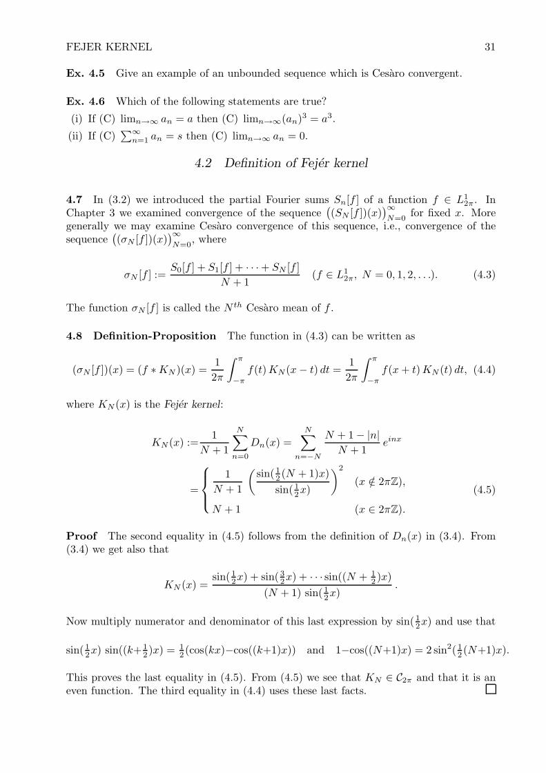
The Fejer Kernels K8, K16, centered at 0, 4π respectively.

4.3 Cesaro convergence of Fourier series

4.9 We need the following three easy consequences of (4.5):

KN (x) ≥ 0 (x ∈ R), (4.6)

1

2π

∫ π

−π

KN (t) dt = 1, (4.7)

KN (x) ≤ 1

(N + 1) sin2( 12x)

≤ π2

(N + 1) x2(0 < |x| ≤ π). (4.8)

4.10 Theorem (Fejer) Let f ∈ L12π, a ∈ R. Suppose that f is continuous in a. Then

limN→∞

(σN [f ])(a) = f(a). (4.9)

Moreover, if f ∈ C2π then the convergence in (4.9) is uniform for a ∈ R.

FEJER KERNEL 33

Proof Let ε > 0. We want to show that |σN (a) − f(a)| < ε for N sufficiently large. Itfollows from (4.4) and (4.7) that

σN (a) − f(a) =1

2π

∫ π

−π

(f(a + t) − f(a)) KN(t) dt.

For any δ ∈ [0, π) we split up the above integral as∫ π

−π=∫|t|<δ

+∫

δ<|t|<π. Then, by use

of (4.6),

|σN (a)−f(a)| ≤ 1

2π

∫ δ

−δ

|f(a+ t)−f(a)|KN(t) dt+1

2π

∫

δ<|t|<π

|f(a+ t)−f(a)|KN(t) dt.

Denote the two successive terms on the right hand side by I1 and I2. First we estimateI1. By the continuity of f in a we can choose δ such that |f(a + t)− f(a)| ≤ 1

2ε if |t| ≤ δ.

Keep this value of δ. Then, by use of (4.7), I1 ≤ 12ε. Next we estimate I2. It follows from

(4.8) that

I2 ≤ π

2(N + 1)

∫

δ<|t|<π

|f(a + t) − f(a)| t−2 dt ≤ π

2(N + 1)δ2

∫ π

−π

(|f(a + t)| + |f(a)|) dt

≤ π2

(N + 1)δ2(‖f‖1 + |f(a)|).

Hence I2 ≤ 12ε for N sufficiently large. This proves the first part of the theorem.

Next assume that f ∈ C2π . Then f is uniformly continuous on R (by the compactnessof [−π, π] and by the 2π-periodicity). Thus we can choose δ such that |f(a+t)−f(a)| ≤ 1

2ε

for all a ∈ R if |t| ≤ δ. With this choice of δ we have I1 ≤ 12ε for all a. Then

I2 ≤ π2

(N + 1)δ2(‖f‖1 + ‖f‖∞).

Hence I2 ≤ 12ε for all a if N is sufficiently large. We conclude that |σN (a) − f(a)| < ε for

all a if N is sufficiently large.

4.11 Corollary (Fejer) Let f ∈ L12π, let a ∈ R, and suppose that the limits

f(a+) := limx↓a

f(x), f(a−) := limx↑a

f(x)

exist. Then we have:

limN→∞

(σN [f ])(a) = 12(f(a+) + f(a−)).

Ex. 4.12 Give the proof of Corollary 4.11 (compare with the proof of Theorem 3.5).

4.13 Theorem 1.11(a) is an immediate corollary of the second statement in Theorem4.10:

34 CHAPTER 4

Corollary (Weierstrass) The space of trigonometric polynomials is dense in C2π withrespect to the norm ‖ . ‖∞.

Proof Let f ∈ C2π. Let ε > 0. Then, by the uniform convergence stated in Theorem4.10, we can take N such that ‖σN [f ]−f‖∞ < ε. Now observe that σN [f ] is a trigonometricpolynomial.

4.14 Corollary Let f ∈ L12π and a ∈ R. Suppose that f is continuous in a. If

limN→∞(SN [f ])(a) exists then this limit is equal to f(a).

Proof By Proposition 4.4 the limit is equal to limN→∞(σN [f ])(a) and hence, by Theorem4.10 to f(a).

4.15 Remark Observe that σN [f ] := f ∗ KN (f ∈ L12π), where KN (N = 0, 1, 2, . . .)

is an even nonnegative function belonging to L12π with properties (2π)−1

∫ π

−πKN (t) dt = 1

and:

For each δ ∈ (0, π): limN→∞

KN (x) = 0 uniformly for δ ≤ |x| ≤ π.

Observe that the proof of Theorem 4.10 only uses these properties of KN and σN [f ].Hence Theorem 4.10 remains valid for any choice of the functions KN satisfying the aboveproperties.

Ex. 4.16 Let f ∈ L12π. Show that limN→∞ σN [f ] = f in L1

2π.Hint Show that limN→∞ ‖σN [f ]− f‖1 = 0 for f ∈ C2π and use that C2π is dense in L1

2π.

4.4 Another approximation theorem of Weierstrass

Corollary 4.13 is an approximation theorem involving trigonometric polynomials. Fromthis we can derive an even more famous approximation theorem of Weierstrass involvingordinary polynomials. (There exist many other proofs of this theorem.) As a tool for theproof we introduce Chebyshev polynomials.

4.17 Definition-Proposition For each nonnegative integer n there is a unique poly-nomial Tn in one variable such that

Tn(cos t) = cos(nt) (t ∈ R). (4.10)

The polynomial Tn has degree n. It is called a Chebyshev polynomial (of the first kind).

Proof For x ∈ [−1, 1] Tn(x) is uniquely determined by (4.10). Hence, if Tn is a polyno-mial then it is unique. Since

cos t cos nt = 12 cos(n + 1)t + 1

2 cos(n − 1)t,

we have

Tn+1(x) = 2x Tn(x) − Tn−1(x) (n = 1, 2, . . .),

while T0(x) = 1, T1(x) = x. Now it follows by induction with respect to n that Tn(x) is apolynomial of degree n in x.

FEJER KERNEL 35

Ex. 4.18 Show that

∫ 1

−1

Tn(x) Tm(x)dx√

1 − x2=

{0, n 6= m,π/2, n = m 6= 0,π, n = m = 0.

Thus the Tn form an orthogonal system in L2((−1, 1); (1− x2)−12 dx). Show also that this

orthogonal system is complete.

Ex. 4.19 Show that for each nonnegative integer n there is a unique polynomial Un(x)of degree n in x such that

Un(cos t) =sin(n + 1)t

sin t(0 6= t ∈ R). (4.11)

Show thatUn+1(x) = 2x Un(x) − Un−1(x) (n = 1, 2, . . .),

while U0(x) = 1, U1(x) = 2x. The polynomial Un is called a Chebyshev polynomial (ofthe second kind). Show that

∫ 1

−1

Un(x) Um(x)√

1 − x2 dx =

{0, n 6= m,π/2, n = m.

Thus the Un form an orthogonal system in L2((−1, 1); (1 − x2)12 dx). Show also that this

orthogonal system is complete.

4.20 Theorem (Weierstrass) Let f ∈ C([a, b]). Then there exists for each ε > 0 apolynomial P in one variable such that |f(x) − P (x)| < ε for x ∈ [a, b].

Proof Without loss of generality we may assume that [a, b] = [−1, 1] (why?). Put g(t) :=f(cos t). Then g ∈ C2π and g is even, so g(n) = g(−n). Hence

(σN [g])(t) = g(0) + 2

N∑

n=1

N + 1 − n

N + 1g(n) cos(nt)

and σN [g] → g for N → ∞, uniformly on R (see Theorem 4.9), so certainly uniformly on[0, π]. Put

fN (x) := g(0) + 2N∑

n=1

N + 1 − n

N + 1g(n) Tn(x).

Then fN (cos t) = (σN [g])(t) and fN (x) is a polynomial of degree ≤ N in x. Since σN [g] → gfor N → ∞, uniformly on [0, π], we have that fN → f as N → ∞, uniformly on [−1, 1].

Ex. 4.21 Let f(x) := |x|. Determine a sequence of polynomials which converges uni-formly to f on [−1, 1].

Ex. 4.22 The analogue of Theorem 4.20 does not hold on R. Give an example of acontinuous function on R which cannot be uniformly approximated by polynomials on R.

36 CHAPTER 4

4.5 Further exercises

Ex. 4.23 For 0 ≤ r < 1 let

Pr(x) :=∞∑

n=−∞

r|n| einx (x ∈ R), (4.12)

the so-called Poisson kernel. For f ∈ L12π put

Ar[f ] := f ∗ Pr. (4.13)

The functions Ar[f ] are known as Abel means. Let a ∈ R and suppose that f is continuousin a. Prove that

limr↑1

(Ar[f ])(a) = f(a). (4.14)

Moreover show that, if f ∈ C2π, the convergence in (4.14) is uniform for a ∈ R.Hint Use Remark 4.15.

Ex. 4.24 Prove that the Gibbs phenomenon cannot occur for the Cesaro and Abel means.That is, if m < f < M , then m < Ar[f ], CN [f ] < M .

37

5 Some applications of Fourier series

5.1 The isoperimetric inequality

5.1 Theorem The area A of a region in the plane which is encircled by a closed non-selfintersecting C1-curve of length L satisfies A ≤ L2/(4π). Equality holds iff the curve isa circle.

Proof Without loss of generality we may assume that L = 2π, and that the curve ispositively oriented and parametrized by its arc length. We may also identify the planewith C. Then the curve has the form t 7→ f(t) with f ∈ C1

2π and with |f ′(t)| = 1 for all

t. Furthermore we may assume without loss of generality that f(0) = 12π

∫ π

−πf(t) dt = 0.

Then we have to show that A ≤ π with equality iff f(t) = ei(t+t0) for some t0 ∈ R. Nowwe have

A(1)= 1

2 Im

∫ 2π

0

f ′(t) f(t)dt = π Im 〈f ′, f〉 ≤ π |〈f ′, f〉|(2)

≤ π ‖f ′‖2 ‖f‖2

(3)= π ‖f‖2

(4)= π ‖f − f(0)‖2

(5)

≤ π ‖f ′‖2

(6)= π. (5.1)

Equality (1) follows from:

Ex. 5.2 Let t 7→ f(t) be a positively oriented closed non-selfintersecting C1-curve in C.

Show that the area of the encircled region equals 12 Im

∫ 2π

0f ′(t) f(t)dt.

Inequality (2) in (5.1) is the Cauchy-Schwarz inequality. Equalities (3) and (6) use that

‖f ′‖2 = 1 by the assumption |f ′(t)| = 1. Equality (4) uses the assumption f(0) = 0.Equality (5) follows from:

Ex. 5.3 Let f ∈ C12π. Show that ‖f − f(0)‖2 ≤ ‖f ′‖2 with equality iff f(n) = 0 for

n 6= −1, 0, 1.

The proof of the last part of Theorem 5.1 is also left as an exercise:

Ex. 5.4 Show that equality everywhere in (5.1) implies that f(t) = ei(t+t0) for somet0 ∈ R.

5.2 The heat equation

5.5 The partial differential equation

∂

∂tF (t, x) = 1

2

∂2

∂x2F (t, x) ((t, x) ∈ (0,∞) × R) (5.2)

is called the heat equation. It is often considered with initial value

F (0, x) = f(x) (x ∈ R) (5.3)

38 CHAPTER 5

for a given function f on R. We will assume that f ∈ C∞2π and we are interested in

a function F which is continuous on [0,∞) × R and C∞ on (0,∞) × R, which satisfiesF (t, x + 2π) = F (t, x) for all t ≥ 0, and which is a solution of (5.2), (5.3). In a suitablenormalization of the variable t we can interprete this as the evolution in time of thetemperature on a ring which is idealized as the unit circle parametrized by its arc length.Then F (t, x) is the temperature at position x and time t. The function f gives the initialtemperature distribution at time t = 0.

Put Ft(x) := F (t, x) and

γn(t) := Ft(n) =1

2π

∫ π

−π

F (t, x) e−inx dx.

Ex. 5.6 Let f ∈ C∞2π and let F be as above. Show the following.

(a) γn is continuous on [0,∞).(b) γn is C∞ on (0,∞) with kth derivative given by

γ(k)n (t) =

1

2π

∫ π

−π

∂kF (t, x)

∂tke−inx dx.

(c) We have

γ′n(t) = −1

2n2γn(t), γn(0) = f(n), γn(t) = f(n) e−

12 n2t.

Ex. 5.7 Let f ∈ C∞2π. Show that

F (t, x) :=

∞∑

n=−∞

f(n) einx− 12 n2t (5.4)

is a well-defined C∞ function on (0,∞) × R, continuous on [0,∞) × R, 2π-periodic in xand satisfying (5.2), (5.3). Conclude that F (t, x) given by (5.4) is the unique solution of(5.2), (5.3) of this type.Hint For the first part use Theorem 2.5(b).

Ex. 5.8 Let F be given by (5.4). Show that∫ π

−π

Ft(x) dx =

∫ π

−π

f(x) dx (t > 0)

(i.e., the total heat on the ring remains constant in time), and

limt→∞

F (t, x) = f(0)

(i.e., the temperature distribution tends to the constant distribution as t → ∞).

Ex. 5.9 Define the heat kernel by

Ht(x) :=∑

n∈Z

einx− 12 n2t (t > 0).

Prove that Ht ∈ C∞2π. Show that, for F given by (5.4), we have Ft = f ∗ Ht (t > 0).

Ex. 5.10 Show that (f ∗ Hs) ∗ Ht = f ∗ Hs+t (s, t > 0) and give a physical explanationof this formula.

APPLICATIONS 39

5.3 Weyl’s equidistribution theorem

5.11 Theorem Let 0 < γ ∈ R \ Q and let 0 ≤ a < b ≤ 1. Then

limn→∞

#{r ∈ N | 0 < r < n, < rγ >∈ [a, b]}n

= b − a.

Here # denotes the number of elements of a set and < x > denotes the fractional partof a positive number x.

Ex. 5.12 Prove this theorem by completing the following outline:

1) Let f ∈ C2π and γ ∈ R \ Q. Prove that

limn→∞

∑nj=1 f(2πjγ)

n=

1

2π

∫ 2π

0

f(t) dt.

a. In case f ≡ 1.b. In case f(t) = eikt, k ∈ Z.c. In case f is a trigonometric polynomial.d. For general f ∈ C2π.

2) Prove that the formula is also valid if f is the periodic extension of the characteristicfunction χ[a,b] of a closed interval [a, b] ⊂ (0, 2π). (Look for continuous functions f1, f2

such that f1 ≤ f ≤ f2 and∫ 2π

0(f2 − f1)(t) dt < ǫ) and apply 1).

Derive the equidistribution theorem.

40

6 Generalities about Fourier integrals

This chapter is the beginning of Part II of the Syllabus. It deals with Fourier integrals.

6.1 In Part I we have seen that, for a 2π-periodic function f which is sufficiently smooth,for instance f ∈ C2

2π, we can write

f(a) =∞∑

n=−∞

(1

2π

∫ π

−π

f(t) e−int dt

)eina (a ∈ R), (6.1)

where the doubly infinite series converges absolutely. Now we will consider functions f onR which are usually not periodic. The analogue of (6.1), valid for sufficiently nice functionsf , is

f(a) =1

2π

∫ ∞

−∞

(∫ ∞

−∞

f(t) e−itx dt

)eixa dx (a ∈ R). (6.2)

If f is a function on R which is sufficiently smooth (say C2) and which decreases sufficientlyfast in absolute value to 0 as t → ∞ (say f(t) = O(|t|−2) as |t| → ∞), then (6.2) holdswith absolutely convergent inner and outer integrals. This we will prove later. For themoment we will only prove (6.2) heuristically from (6.1).

6.2 Let f be a C2-function on R with compact support and let a ∈ R. We will give aheuristic proof of (6.2). For λ > 0 such that supp(f) ⊂ [−λπ, λπ] and |a| ≤ πλ define afunction fλ ∈ C2

2π such that fλ(t) := f(λt) if −π ≤ t ≤ π. It follows from (6.1) that

f(a) = fλ(a/λ) =1

2π

∞∑

n=−∞

(∫ π

−π

f(λt) e−int dt

)eina/λ

=1

2π

∞∑

n=−∞

(∫ ∞

−∞

f(t) e−int/λ dt

)eina/λ λ−1

=1

2π

∑

x∈λ−1Z

(∫ ∞

−∞

f(t) e−ixt dt

)eixa λ−1

=1

2πlim

N→∞

∑

x∈λ−1Z∩[−N,N ]

f(x) eixa λ−1, (6.3)

where we have put

f(x) :=

∫ ∞

−∞

f(t) e−ixt dt (x ∈ R). (6.4)

The sum in (6.3) can be considered as a Riemann sum for the partition of [−N, N ] into

equidistant points with distance λ−1. Since the function x 7→ f(x) eixa is continuous, thisRiemann sum tends to the corresponding integral. So formally the limit of (6.3) as λ → ∞equals

1

2πlim

N→∞

∫ N

−N

f(x) eixa dx,

which is equal to the right hand side of (6.2). It has to be justified that we may take thelimit for λ → ∞ in (6.3) inside the limit for N → ∞. We will skip this here.

GENERALITIES 41

6.3 Definition Let f ∈ L1(R). Then the integral on the right hand side of (6.4) is

absolutely convergent since |f(t) e−ixt| ≤ |f(t)|. So (6.4) yields a well-defined function f

on R. We call the transform f 7→ f given by (6.4) the Fourier transform. The function f

is called the Fourier transform of f . Note that f only depends on the equivalence class off . So the function f is well-defined for f ∈ L1(R).

Ex. 6.4 Let [a, b] be a closed bounded interval and let f := χ[a,b] be its characteristicfunction. Show the following: f ∈ L1(R) and

f(x) =

e−iax − e−ibx

ix=

2 sin( 12(b − a)x) e−

12 i(a+b)x

xif x 6= 0,

b − a if x = 0.

Observe from this result that f is continuous and that limx→±∞ f(x) = 0.

Ex. 6.5 Let f(x) = 11+x2 on R. Compute f . (Use Contour integration.)

6.6 Let p ∈ [1,∞), in particular we will consider p = 1 or 2. We write

‖f‖p :=

(∫ ∞

−∞

|f(t)|p dt

)1/p

if f ∈ Lp(R) or f ∈ Lp(R),

and we put

‖f‖∞ := supx∈R

|f(x)| if f is a bounded continuous function on R.

Let Cc(R) denote the space of complex-valued continuous functions on R with compactsupport. The following Proposition is proved in Rudin, Theorem 3.14.

6.7 Proposition Let p ∈ [1,∞). Then Cc(R) is dense in Lp(R).

Ex. 6.8 A function f : R → C is called simple if it is a linear combination of characteristicfunctions of bounded intervals. Equivalently, f is simple if there are real numbers a1 <a2 < . . . < an such that f vanishes outside [a1, an] and f is constant on each interval(ai, ai+1) (i = 1, . . . , n − 1).

Let p ∈ [1,∞). Prove, by using Proposition 6.7, that the space of simple functions is densein Lp(R).

6.9 Theorem Let f ∈ L1(R). Then

(a) f is a bounded continuous function on R.

(b) ‖f‖∞ ≤ ‖f‖1.

(c) limx→±∞ f(x) = 0 (Riemann-Lebesgue Lemma).

42 CHAPTER 6

Proof For the proof of the continuity of f note that, for x ∈ R,

limy→x

∫ ∞

−∞

f(t) e−iyt dt =

∫ ∞

−∞

(limy→x

f(t) e−iyt)

dt =

∫ ∞

−∞

f(t) e−ixt dt

by Lebesgue’s dominated convergence theorem (syll. Integratietheorie) since |f(t) e−iyt| ≤|f(t)| and

∫∞

−∞|f(t)| dt < ∞. Clearly, it follows from (6.4) that

|f(x)| ≤∫ ∞

−∞

|f(t)| dt = ‖f‖1 (x ∈ R).

This settles (a) and (b).For the proof of (c) first note that the result is valid if f is a simple function. This

follows from Exercise 6.4. Now let f ∈ L1(R). Let ε > 0. By Exercise 6.8 there is a simple

function g such that ‖f − g‖1 < ε/2. By (b) we have that |f(x) − g(x)| < ε/2. Hence

|f(x)| ≤ ε/2 + |g(x)| and there is M > 0 such that |g(x)| < ε/2 if |x| > M .

Ex. 6.10 Let

C0(R) := {f : R → C | f is continuous and limx→±∞

f(x) = 0}.

Prove that C0(R) is a closed linear subspace of the Banach space of bounded continuousfunctions on R with respect to the sup-norm, so C0(R) is a Banach space itself with respect

to the sup-norm. Also observe that the map f 7→ f : L1(R) → C0(R) is a bounded linearoperator.

Ex. 6.11 Let f ∈ L1(R), a ∈ R, c ∈ R\{0}. Prove the following.

(a) If g(t) := f(t + a) then g(x) = eiax f(x).

(b) If g(t) := eiat f(t) then g(x) = f(x − a).

(c) If g(t) := f(ct) then g(x) = |c|−1 f(c−1x).

(d) In particular, if g(t) := f(−t) then g(t) = f(−t).

6.12 Proposition Let f, g ∈ L1(R). Then

∫ ∞

−∞

f(x) g(x) dx =

∫ ∞

−∞

f(x) g(x) dx.

(Both integrals converge absolutely because of Theorem 6.9(a).)

Proof We have to show that

∫ ∞

x=−∞

(∫ ∞

y=−∞

f(x) e−ixy g(y) dy

)dx

is equal to ∫ ∞

y=−∞

(∫ ∞

x=−∞

f(x) e−ixy g(y) dx

)dy.

GENERALITIES 43

This follows from the Fubini Theorem 2.14 since∫ ∞

x=−∞

(∫ ∞

y=−∞

|f(x) e−ixy g(y)| dy

)dx < ∞.

6.13 Proposition Let f ∈ C1(R) such that f, f ′ ∈ L1(R). Then

(f ′)(x) = ix f(x), (6.5)

and f(x) = o(|x|−1) as x → ±∞.

Proof Let M > 0. Integration by parts shows that

∫ M

−M

f ′(t) e−ixt dt = e−ixM f(M)− eixM f(−M) + ix

∫ M

−M

f(t) e−ixt dt.

Then (6.5) will follow by letting M → ∞ in the above formula, provided we can showthat limM→∞ f(±M) = 0. These last limits are indeed valid. For instance, f(M) =

f(0) +∫M

0f ′(t) dt. Hence f(∞) := limM→∞ f(M) = f(0) +

∫∞

0f ′(t) dt exists. Then

necessarily f(∞) = 0, since otherwise∫∞

−∞|f(t)| dt = ∞.

The second statement follows by combination with Theorem 6.9(c).

6.14 Proposition Let f ∈ L1(R) such that the function g: x 7→ xf(x) is in L1(R).

Then f is differentiable on R with ( f )′ = −ig.

Proof Let a, b ∈ R with a < b. Then, by Proposition 6.12 and Exercise 1.4,

∫ b

a

g(x) dx =

∫ ∞

−∞

g(x) χ[a,b](x) dx

=

∫ ∞

−∞

g(x) (χ[a,b])(x) dx

=

∫ ∞

−∞

xf(x)e−iax − e−ibx

ixdx

= i

∫ ∞

−∞

f(x)(e−ibx − e−iax) dx = i(f(b) − f(a)).

Hencef(a + h) − f(a)

h= −ih−1

∫ a+h

a

g(x) dx.

Now let h → 0 and use the fact that g is continuous.

6.15 Corollary

(a) Let f ∈ Ck(R) such that f, f ′, . . . , f (k) ∈ L1(R). Then (f (k))(x) = (ix)k f(x) and

f(x) = o(|x|−k) as x → ±∞.(b) Let f be a Lebesgue measurable function on R such that

∫∞

−∞(1 + |t|)k |f(t)| dt < ∞.

Then f ∈ Ck(R) and ( f )(k)(x) =∫∞

−∞(−it)k f(t) e−ixt dt.

(c) Let α ∈ R with α > 1. Let f be a Lebesgue measurable function on R such that

f(x) = O(|x|−α) for |x| → ∞. Then f ∈ Ck(R) if k + 1 < α.

44 CHAPTER 6

Observe the general rules:• Faster decrease of |f(t)| to 0 as |t| → ∞ implies more smoothness of f .

• More smoothness of f implies faster decrease of |f(x)| to 0 as |x| → ∞.

6.16 We introduce the following notation for some operators acting on functions on R:

(Df)(x) := f ′(x) (differentiation),

(Mf)(x) := x f(x) (multiplication),

(Taf)(x) := f(x + a) (translation),

(Eaf)(x) := eiax f(x) (exponential multiplication),

(Pf)(x) := f(−x) (parity operator).

Some of the previous results can now be summarized in the following table:

g g

Df iMf

Mf iDf

Eaf T−af

Taf Eaf

t 7→ f(ct) x 7→ |c|−1f(c−1x)

Pf P f

6.17 Definition S is the set of all f ∈ C∞(R) such that, for all nonnegative integersn, m the function x 7→ xn f (m)(x) is bounded.

So S consists of the C∞-functions f on R such that f and all its derivatives arerapidly decreasing to 0 as the argument tends to ±∞. Briefly we call such functionsrapidly decreasing C∞-functions on R. This class of functions was introduced by LaurentSchwartz. He used this as a class of test functions for his so-called tempered distributions.

The (immediate) proofs of the following statements are left to the reader.

6.18 Proposition S is a linear space. If f ∈ S then the functions Df , Mf , Eaf , Taf ,x 7→ f(cx) and Pf are also in S. If f ∈ S then f ∈ S.

Ex. 6.19 Let f(t) := e−12 t2 (the Gaussian function). Show the following:

(a) f ∈ S.

(b) Df = −Mf , Df = −Mf .

(c) f(x) = C e−12x2

with C =∫∞

−∞e−

12 x2

dx =√

2π.

Hint Solve the differential equation for f in (b).

Ex. 6.20 Let f(t) := e−12 t2 . Then

f(x) =

∫ ∞

−∞

e−12 t2 e−ixt dt = e−

12 x2

∫ ∞

−∞

e−12 (t+ix)2 dt (x ∈ R).

Derive from this formula the result of Exercise 6.19(c), by contour integration.

GENERALITIES 45

Ex. 6.21 Let f ∈ L1(R). Suppose that f has compact support, i.e., f vanishes outsidesome bounded interval. Prove the following.(a) If f = 0 then f = 0 a.e..

Hint Reduce this to the case of periodic functions.(b) The function f is the restriction to R of an entire analytic function on C (the function

given by (6.4) for x ∈ C).

(c) If f also vanishes on R outside some bounded interval then f = 0 a.e..

6.22 Definition-Theorem For f, g ∈ L1(R) the convolution product f ∗ g is definedby

(f ∗ g)(x) :=

∫ ∞

−∞

f(y) g(x− y) dy (x ∈ R). (6.6)

Then the integral in (6.6) converges absolutely for almost all x ∈ R and f ∗ g ∈ L1(R).Furthermore,

‖f ∗ g‖1 ≤ ‖f‖1 ‖g‖1 (6.7)

and(f ∗ g)(x) = f(x) g(x). (6.8)

Proof Analogous to the proof of Definition-Theorem 2.19. Use the Fubini Theorem 2.14.

Ex. 6.23 Let p(x) be a polynomial with real coefficients in the real variable x. Findnecessary and sufficient conditions in order that the function x 7→ ep(x) belongs to S.

46

7 Inversion formula

7.1 (Dirichlet kernel) Let f ∈ L1(R), ω > 0. Put

(Iω[f ])(s) :=1

2π

∫ ω

−ω

f(x) eixs dx (s ∈ R). (7.1)

In view of (6.2) we expect (but still have to prove) that Iω[f ] → f as ω → ∞. Theadvantage of (7.1) compared to the corresponding integral from −∞ to ∞ is that it can bewritten as an integral transformation (of convolution type) acting on f with very simpleintegral kernel: the Dirichlet kernel

sin(ωt)

πt=

1

2π

∫ ω

−ω

e−ixt dx. (7.2)

Proposition We have

(Iω[f ])(s) =

∫ ∞

−∞

f(t + s)sin(ωt)

πtdt, (7.3)

∣∣∣∣sin(ωt)

πt

∣∣∣∣ ≤ ω/π (t ∈ R), (7.4)

∫ ∞

−∞

sin(ωt)

πtdt =

2

π

∫ ∞

0

sin t

tdt = 1 (7.5)

(the last two integrals converging but not absolutely converging).

The proof of these formulas is left to the reader. For the proof of (7.3) substitute (6.4)into (7.1) and interchange the two integrals (allowed by Fubini’s theorem; check this).

7.2 The following results are analogous to §3.2. We give a convergence criterium forFourier inversion in a certain point.

Theorem Let f ∈ L1(R), a ∈ R. Suppose that one of the following two conditions holds:

(a) There are M, α, δ > 0 such that

|f(a + x) − f(a)| < M |x|α for |x| < δ.

(b) f is continuous in a and also right and left differentiable in a.

Then we have:lim

ω→∞(Iω[f ])(a) = f(a). (7.6)

Proof Condition (b) implies condition (a), so we may assume Condition (a). We have

(Iω[f ])(a)− f(a)

∫ 1

−1

sin(ωx)

πxdx

=

∫ 1

−1

f(a + x) − f(a)

πxsin(ωx) dx +

∫

|x|>1

f(a + x)

πxsin(ωx) dx. (7.7)

INVERSION FORMULA 47

Since ∫ 1

−1

sin(ωx)

πxdx =

∫ ω

−ω

sin y

πydy −→ 2

π

∫ ∞

0

sin y

ydy = 1 as ω → ∞,

it is sufficient to prove that the right hand side tends to 0 as ω → ∞. However, we willsee that the right hand side is of the form π−1

∫∞

−∞g(x) sin(ωx) dx with g ∈ L1(R), so it

tends to 0 as ω → ∞ because of the Riemann-Lebesgue lemma (see Theorem 6.9(c)).The claim about the right hand side is proved by splitting it up as a sum of three

terms (where we assume that δ < 1):

|x| < δ: |g(x)| =∣∣∣∣f(a + x) − f(a)

x

∣∣∣∣ < M |x|α−1,

δ ≤ |x| < 1: |g(x)| =∣∣∣∣f(a + x) − f(a)

x

∣∣∣∣ ≤ δ−1(|f(a + x)| + |f(a)|),

|x| ≥ 1: |g(x)| =∣∣∣∣f(a + x)

x

∣∣∣∣ ≤ |f(a + x)|.

7.3 Theorem Let f ∈ L1(R), let a ∈ R, and suppose that the limits

f(a+) := limx↓a

f(x), f(a−) := limx↑a

f(x)

exist. Suppose that one of the two following conditions holds:

(a) There are M, α, δ > 0 such that

|f(a + x) − f(a+)| ≤ Mxα and |f(a − x) − f(a−)| ≤ Mxα for 0 < x < δ.

(b) f is right and left differentiable in a in the sense that the following two limits exist:

f ′(a+) := limy↓0

f(a + y) − f(a+)

y, f ′(a−) := lim

y↓0

f(a − y) − f(a−)

−y.

Then we have:

limω→∞

(Iω[f ])(a) = 12 (f(a+) + f(a−)).

Ex. 7.4 Prove Theorem 7.3 as a corollary of Theorem 7.2, analogous to the proof ofTheorem 3.5.

7.5 Corollary (localization principle) Let f, g ∈ L1(R), let a ∈ R, and supposethat f(x) = g(x) for x in a certain neighbourhood of a. Then precisely one of the followingtwo alternatives holds for the behaviour of (Iω[f ])(a) and (Iω[g])(a) as ω → ∞:

(a) Both limits exist and are equal:

limω→∞

(Iω[f ])(a) = limω→∞

(Iω[g])(a)

(b) Neither (Iω[f ])(a) nor (Iω[g])(a) has a limit as ω → ∞.

48 CHAPTER 7

Thus, if for some f ∈ L1(R) and some a ∈ R the inversion formula (7.6) holds, thenthis inversion formula remains valid if f is perturbed within L1(R) such that f remainsunchanged on some neighbourhood of a.

Ex. 7.6 Prove Corollary 7.5.

7.7 Corollary Let f ∈ L1(R) such that also f ∈ L1(R) and f is differentiable on R.

Then (f ) is well-defined and

(f ) (s) = 2π f(−s) (s ∈ R).

Ex. 7.8 Prove Corollary 7.7. Can the differentiability assumption be relaxed?

Ex. 7.9 (van Rooij, Voorbeeld 15.8) Define f : R → R by

f(x) :=

{1 − |x| if |x| ≤ 1,0 if |x| > 1.

(a) Show that f ∈ L1(R) and f(x) = 2x−2(1 − cos x) (x 6= 0), f(0) = 1.

(b) Show that f ∈ L1(R) and that (f ) (a) = 2π f(−a) for all a ∈ R.

(c) Show that ∫ ∞

−∞

1 − cos x

x2dx = π.

Ex. 7.10 Let

f(t) :=

12− t if 0 < t ≤ 1

2,

−12 − t if −1

2 ≤ t < 0,0, otherwise.

Compute f(x). Examine the behaviour of f(x) as |x| → ∞.

Ex. 7.11 Let f be continuously differentiable on R\{0}. Suppose that f, f ′ ∈ L1(R) andthat the following four limits exist:

a := limt↓0

f(t), b := limt↑0

f(t), limt↓0

f(t) − a

t, lim

t↑0

f(t) − b

t.

(a) Show that f(x) = O(|x|−1) as |x| → ∞.

(b) Show that f(x) = o(|x|−1) as |x| → ∞ iff a = b.

Ex. 7.12 Let

f(t) :=

{(1 − t2)α− 1

2 if |t| < 1,0 if |t| ≥ 1.

Assume that Re α > −12 . Show that

f(x) =Γ( 1

2 ) Γ(α + 12)

Γ(α + 1)

∞∑

k=0

(−x2/4)k

k! (α + 1)k,

where (α + 1)k := (α + 1)(α + 2) . . . (α + k).

What can be concluded about the speed with which |f(x)| tends to 0 as |x| → ∞?

49

8 L2 theory

We will work now with the space L2(R) of square integrable functions on R and with theHilbert space L2(R) of equivalence classes of such functions. Inner product and norm aregiven by

< f, g >:=

∫ ∞

−∞

f(x) g(x)dx, ‖f‖2 := (〈f, f〉) 12 =

(∫ ∞

−∞

|f(x)|2 dx

) 12

. (8.1)

The space S (see Definition 6.17) is a linear subspace of L2(R).We will now denote by F a slightly renormalized version of the Fourier transform

f 7→ f :

(Ff)(x) :=1√2π

f(x) =1√2π

∫ ∞

−∞

f(t) e−ixt dt. (8.2)

Here f ∈ L1(R), in particular we will take f ∈ S.

8.1 Proposition The map F :S → S is a linear bijection, with inverse

(F−1g)(s) = (Fg)(−s) (g ∈ S). (8.3)

Furthermore F preserves the inner product (8.1) on S:

〈Ff,Fg〉 = 〈f, g〉 (f, g ∈ S). (8.4)

For convenience we give also more extended versions of (8.3) and (8.4):

(F−1g)(s) =1√2π

∫ ∞

−∞

g(x) eisx dx, (8.5)

∫ ∞

−∞

f(t) g(t)dt =

∫ ∞

−∞

(Ff)(x) (Fg)(x)dx =1

2π

∫ ∞

−∞

f(x) g(x) dx. (8.6)

The proof of this Proposition is immediate, in view of Corollary 7.7, Proposition 6.18and Proposition 6.12.

8.2 We will now introduce some special C∞ functions, which we will need as tools (seealso van Rooij, §18.1).

Let a < b and put

f(x) :=

exp

(1

x − b− 1

x − a

)if a < x < b,

0, otherwise.

Then f ∈ C∞(R) and f(x) ≥ 0 for all x ∈ R.Let

F (x) :=(∫ x

a

f(t) dt)/(∫ b

a

f(t) dt).

Then F ∈ C∞(R), F (x) = 0 if x ≤ a, F (x) = 1 if x ≥ b, and F is strictly increasing on[a, b].

50 CHAPTER 8

Ex. 8.3 Let [a, b] be a closed bounded interval and χ[a,b] its characteristic function. Showthat χ[a,b] can be approximated arbitrarily closely in L2 norm by functions in S.

8.4 Proposition The space S is dense in L2(R).

Proof By Exercise 6.8 the simple functions are dense in L2(R). Next use Exercise 8.3.

8.5 As a corollary of the previous propositions we obtain:

Theorem (Parseval-Plancherel) The map F :S → S has a unique extension to acontinuous linear map F : L2(R) → L2(R). This extension is an isometry of Hilbert spaces:

〈Ff,Fg〉 = 〈f, g〉 (f, g ∈ L2(R)),

it is bijective, and it satisfies

(F2f)(s) = f(−s) a.e.

We have obtained two definitions of the Fourier transform, which we will denote byF1 resp. F2 for the moment:

(F1f)(x) :=1√2π

∫ ∞

−∞

f(t) e−ixt dt (f ∈ L1(R)),

(F2f)(x) :=(L2) limn→∞

F1fn, where Fn ∈ S and (L2) limn→∞

fn = f .

For f ∈ L1(R) ∩ L2(R) it will turn out that F1f = F2f .

Lemma Let f ∈ L1(R) ∩ L2(R). Then there is a sequence (fn)∞n=1 in S such that‖f − fn‖1 → 0 and ‖f − fn‖2 → 0 as n → ∞.

Proof Let ε > 0. There exists M > 1 such that ‖fχ[−M,M ] − f‖p < ε for p = 1, 2. Write

g := fχ[−M,M ]. Then there exists h ∈ S such that ‖g−h‖2 < ε/(2√

M) < ε. We can evenchoose h in this way such that it has support within [−2M, 2M ] (why?). Thus

‖g − h‖1 =

∫ 2M

−2M

|g(x) − h(x)| dx ≤ 2√

M ‖g − h‖2 < ε.

Hence ‖f − h‖1 < 2ε and ‖f − h‖2 < 2ε.

8.6 Theorem If f ∈ L1(R) ∩ L2(R) then F1f = F2f .

Proof Take a sequence (fn)∞n=1 in S such that ‖f−fn‖1 → 0 and ‖f−fn‖2 → 0 if n → ∞.Then F2f = limn→∞ F1fn in L2(R). Since

√2π ‖F1f − F1fn‖∞ ≤ ‖f − fn‖1, it follows

that (F1f)(x) = limn→∞(F1fn)(x) pointwise. From integration theory we know that aconvergent sequence in L2(R) always has a subsequence which converges almost everywhereto the limit function. Hence the sequence (F1fn)∞n=1 has a subsequence (F1fnk

)∞k=1 suchthat

(F2f)(x) = limk→∞

(F1fnk)(x) = (F1f)(x) a.e.

L2 THEORY 51

8.7 Theorem If f ∈ L2(R) then

(Ff)(x) = (L2) limM→∞

1√2π

∫ M

−M

f(t) e−ixt dt,

which can be rewritten as

limM→∞

∫ ∞

−∞

∣∣∣(Ff)(x)− 1√2π

∫ M

−M

f(t) e−ixt dt∣∣∣2

dx = 0.

Proof ‖f−fχ[−M,M ]‖2 → 0 if M → ∞. Hence ‖F2f−F2(fχ[−M,M ])‖2 → 0 as M → ∞.

Because fχ[−M,M ] ∈ L1(R) ∩ L2(R), it follows that F2(fχ[−M,M ]) = F1(fχ[−M,M ]).

Ex. 8.8 (van Rooij, Opgave 19.A) Show that not L1(R) ⊂ L2(R). But show that allbounded functions in L1(R) lie in L2(R).

Ex. 8.9 (van Rooij, Voorbeeld 19.9) Use the Fourier transform computed in Exercise7.9 in order to show that ∫ ∞

−∞

(sin t

t

)4

dt =2π

3.

Ex. 8.10 (van Rooij, Opgave 19.B) Let f, g ∈ L2(R). Then fg ∈ L1(R), thus f g

exists. Take representatives in L2(R) of f , g ∈ L2(R) and denote these representatives also

by f , g. Show that

2π fg(x) =

∫ ∞

−∞

f(t) g(x − t) dt.

Ex. 8.11 (van Rooij, Opgave 19.E) For n a nonnegative integer define the functionhn ∈ S and the Hermite polynomial Hn by

hn(x) := (x − d/dx)n e−x2/2, Hn(x) := ex2/2 hn(x).

Prove the following.

(a) We have

Hn+1(x) = 2x Hn(x) − H ′n(x) and Hn(x) = (−1)n ex2

(d/dx)n e−x2

.

Hn is a polynomial of degree n with real coefficients; the term of degree n in Hn hascoefficient 2n.

(b) hn = (−i)n√

2π hn. (Thus hn is an eigenfunction of the Fourier transform L2(R) →L2(R).)

(c) If n 6= m then 〈hn, hm〉 = 0. (So the functions hn form an orthogonal system inL2(R).)

Hint Let n > m. Substitute hn(x) = (−1)n ex2/2 (d/dx)n e−x2

, hm(x) = e−x2/2 Hm(x),and perform integration by parts.

52 CHAPTER 8

(d) If f ∈ L2(R) and 〈f, hn〉 = 0 for all n, then f(x) = 0 a.e.. (So the functions hn forma complete orthogonal system in L2(R).)

Hint For each polynomial P we have∫∞

−∞f(x) e−x2/2 P (x) dx = 0. By the domi-

nated convergence theorem this implies that

∫ ∞

−∞

f(x) e−x2/2e−ixy dx = 0.

Ex. 8.12 (For this exercise use results from both Fourier series and Fourier integrals.)Below define x−1 sin x for x = 0 by continuity.

(a) Let t ∈ R. Show that for each x ∈ (−π, π) we have

∞∑

n=−∞

sin(π(t − n))

π(t − n)einx = eixt

with pointwise convergence. What is the evaluation of the sum on the left hand sidefor other real values of x?

(b) Show that, for all n, m ∈ Z, we have

∫ ∞

−∞

sin(π(t − n))

π(t − n)

sin(π(t − m))

π(t − m)dt = δn,m,

where the integral converges absolutely.

(c) Does there exist f ∈ L2(R) with f 6= 0 such that

∫ ∞

−∞

f(t)sin(π(t − n))

π(t − n)dt = 0 for all n ∈ Z ?

(d) Let f ∈ L2([−π, π]). Extend f , defined as a function on Z by (1.8), to a function onR by

f(t) :=1

2π

∫ π

−π

f(x) e−ixt dx (t ∈ R).

Show that

f(t) =

∞∑

n=−∞

f(n)sin(π(t − n))

π(t − n)(t ∈ R)

with absolutely convergent sum.

53

9 Poisson summation formula

The Poisson summation formula is an equality of two doubly infinite sums over sets ofequidistant points in R. The first sum involves a function f on R, the second one itsFourier transform f .

9.1 Theorem Let f ∈ L1(R)∩C(R) such that f(t) = O(|t|−2) as |t| → ∞ and f(x) =O(|x|−2) as |x| → ∞. (Take for instance f ∈ S.) Then

∞∑

l=−∞

f(x + 2πl) =1

2π

∞∑

k=−∞

f(k) eikx (x ∈ R), (9.1)

where the series on both sides pointwise and absolutely converge to a function in C2π (i.e.,to a 2π-periodic continuous function).

Proof Put

gN (x) :=

N∑

l=−N

f(x + 2πl), g(x) := limN→∞

gN (x) =

∞∑

l=−∞

f(x + 2πl).

The last series converges pointwise and absolutely on R because f(x) = O(|x|−2) as |x| →∞. This series even converges uniformly for x in a compact subset of R. Hence g iscontinuous on R. Clearly, g is also 2π-periodic. Next observe that

|gN(x)| ≤∞∑

l=−∞

|f(x + 2πl)| and

∫ π

−π

(∞∑

l=−∞

|f(x + 2πl)|)

dx =

∫ ∞

−∞

|f(y)| dy < ∞.

This justifies an application of the dominated convergence theorem as follows (k ∈ Z):

∫ π

−π

g(x) e−ikx dx = limN→∞

∫ π

−π

gN (x) e−ikx dx

= limN→∞

∫ (2N+1)π

−(2N+1)π

f(y) e−iky dy =

∫ ∞

−∞

f(y) e−iky dy = f(k).

Hence, because f(k) = O(|k|−2) as |k| → ∞, we conclude that g(x) equals the right handside of (9.1).

Specialization of (9.1) yields

∞∑

l=−∞

f(2πl) =1

2π

∞∑

k=−∞

f(k). (9.2)

Here f is as in Theorem 9.1 and there is absolute convergence on both sides.

54 CHAPTER 9

Ex. 9.2 Let f be as in Theorem 9.1. Assume c > 0. Prove the following identities.

(a)∞∑

l=−∞

f(x + 2πc l) =1

2πc

∞∑

k=−∞

f(c−1k) eikc−1x,

(b)

∞∑

l=−∞

f(2πc l) =1

2πc

∞∑

k=−∞

f(c−1k),

(c)

∞∑

l=−∞

e−12 (x+2πc l)2 =

1

c√

2π

∞∑

k=−∞

e−12 c−2k2

eikc−1x,

(d)∞∑

l=−∞

e−π(x+c l)2 = c−1∞∑

k=−∞

e−πc−2k2

e2πikc−1x,

(e)

∞∑

l=−∞

e−πc2l2 = c−1∞∑

k=−∞

e−πc−2k2

.

Ex. 9.3 Show that (d) and (e) of Exercise 9.2 remain valid if c, x ∈ C with | arg c2| < π/2.One of the theta functions is defined by

ϑ3(z | τ) :=

∞∑

n=−∞

eiπτn2

e2inz (Im τ > 0, z ∈ C).

Use (d) of Exercise 9.2 in order to show that

τ− 12 exp

(−z2/(πτ)

)ϑ3(τ

−1z | τ−1i) = ϑ3(z | iτ) (Re τ > 0, z ∈ C).

Ex. 9.4 (van Rooij, Opgave 14.A) Show that

∑

n∈Z

1

n2 + β2=

π

β

cosh πβ

sinhπβ(β > 0).

Hint Apply (9.2) with f(x) := e−β|x|.

Ex. 9.5 Apply (9.2) with f as in Exercise 7.10 in order to show that

∞∑

m=−∞

1

(x + m)2=

π2

(sinπx)2(x ∈ R\Z).

55

10 Some applications of Fourier integrals

10.1 Heisenberg’s inequality

10.1 Lemma Let V be a complex vector space with hermitian inner product 〈 . , . 〉 andwith linear operators A, B: V → V such that 〈Af, g〉 = −〈f, Ag〉 and 〈Bf, g〉 = −〈f, Bg〉for all f, g ∈ V . Then

∣∣〈 12i (AB − BA)f, f〉

∣∣ ≤ ‖Af‖ ‖Bf‖ (f ∈ V ). (10.1)

For given f ∈ V equality holds in (10.1) iff Af = iλBf for some λ ∈ R or Bf = 0.

Proof Observe that

〈 12i (AB − BA)f, f〉 = −1

2i

(〈Bf, Af〉 − 〈Af, Bf〉

)= Im

(〈Af, Bf〉

)

and ∣∣Im(〈Af, Bf〉

)∣∣ ≤∣∣〈Af, Bf〉

∣∣ ≤ ‖Af‖ ‖Bf‖.

10.2 We now discuss a special case of the above lemma. Take V := S, Af := f ′,(Bf)(x) := ixf(x). Then

12i

((AB − BA)f

)(x) = 1

2f(x).

Hence

12≤ 1

‖f‖2

(∫ ∞

−∞

x2 |f(x)|2 dx

) 12 1

‖f ‖2

(∫ ∞

−∞

y2 |f(y)|2 dy

) 12

(f ∈ S). (10.2)

For given f ∈ S equality holds in (10.2) iff f ′(x) = −λ x f(x) for some λ ∈ R, i.e., iff

f(x) = const. e−12 λx2

for some λ > 0. (For λ ≤ 0 the function f is not in S.)As a corollary of (10.2) we find that for f ∈ S, x0, y0 ∈ R the following inequality

holds:

12 ≤ 1

‖f‖2

(∫ ∞

−∞

(x − x0)2 |f(x)|2 dx

) 12 1

‖f ‖2

(∫ ∞

−∞

(y − y0)2 |f(y)|2 dy

) 12

. (10.3)

For fixed f ∈ S the right hand side of (10.3) attains its absolute minimum for

x0 = µ(f) :=

∫∞

−∞x |f(x)|2 dx

∫∞

−∞|f(x)|2 dx

, y0 = µ(f ) :=

∫∞

−∞y |f(y)|2 dy

∫∞

−∞|f(y)|2 dy

.

Here µ(f) is the mean value of the stochastic variable x with respect to the probability

distribution(∫∞

−∞|f(x)|2 dx

)−1 |f(x)|2 dx on R and µ(f ) is the mean value of the stochastic

variable y with respect to the probability distribution(∫∞

−∞|f(y)|2 dy

)−1 |f(y)|2 dy on R.Denote the corresponding variances by

σ(f) :=1

‖f‖2

(∫ ∞

−∞

(x − µ(f)

)2 |f(x)|2 dx

) 12

,

σ(f ) :=1

‖f ‖2

(∫ ∞

−∞

(y − µ(f )

)2 |f(y)|2 dy

) 12

.

56 CHAPTER 10

Then we finally obtain Heisenberg’s inequality

σ(f) σ(f ) ≥ 12 . (10.4)

Thus the two stochastic variables x and y cannot be concentrated both on arbitrarily smallintervals.

Heisenberg’s inequality is better known as Heisenberg’s uncertainty relation when in-terpreted in quantum mechanics or in signal analysis. In quantum mechanics the variablesx and y are the position and impulse operator, respectively, for a one-dimensional particle.Then position and impulse cannot be both measured with arbitrary accuracy. In signalanalysis x is the time and y is the frequency of a signal. Here time and frequency cannotboth be measured with arbitrary accuracy.

Ex. 10.3 Let f ∈ S, ‖f‖2 = 1, α, β, a, b > 0, (α + a2)(β + b2) < 14 . Show that it is

impossible that the following two inequalities hold together:∫

|x|>a

x2 |f(x)|2 dx < α and

∫

|y|>b

y2 |f(y)|2 < 2πβ.

10.2 Fourier Transform on finite cyclic groups

The impact of the seemingly pure mathematical topic of this section on numerical andapplied mathematics cannot be overestimated. In the present section all relevant groupswill be finite. We can endow such group with the discrete topology (all subsets are open)and obtain what is called a topological group.

For completeness, we mention here that a topological group is a group endowed witha topology such that the group operations multiplication and inversion are continuous. Inparticular the notion of a continuous function on a topological group is available. Importantexamples of topological groups are Rn and Cn with the Euclidean topology. We will notpursue the implications of this notion at all, but we will use the terminology in the followingsense. The definitions will always be for a topological group G, in the results the groupwill always be finite. As a consequence, we will speak of continuous mappings of our finitegroups, although this is strictly speaking superfluous: all mappings of a discrete topologicalspace are continuous. However, using the terminology as we do, it will fit perfectly in thegeneral framework of topological and Lie groups.

10.4 Let N ∈ N, set ωN = e2πi/N . We introduce

GN = 〈ωN 〉 = {ωkN , k = 1, . . . , N}.

Thus GN is the multiplicative cyclic subgroup of order N of the circle group T = {z ∈ C :|z| = 1} ⊂ C. The relative topology on GN , inherated from the Euclidean topology on C

is discrete.Next C(G) denotes the vector space of the continuous complex valued functions on a

topological group G. Of course C(GN ) may be identified with CN .A character on a group G is a continuous homomorphism from G to T . The set of

characters on G form a group, denoted by G with multiplication

e1e2(g) = e1(g)e2(g), ei ∈ G, g ∈ G.

Ex. 10.5 Show that G is indeed a group. What is its unit element? Can you describethe inversion?

APPLICATIONS OF FOURIER INTEGRALS 57

10.6 Lemma

GN∼= GN .

Proof Define α : GN → GN by

(α(ωjN ))(ωk

N ) = ωkjN .

One can check easily that α is an injective homomorphism. It is also surjective: If e ∈ GN ,then e(ωk

N ) = (e(ωN ))k ∈ T for all integers k. Since (e(ωN ))N = e(id) = 1, we conclude

that e(ωN ) = ωjN for some j ∈ 1, .., N . It then follows that e = α(ωj

N ).

10.7 As C(GN ) ∼= CN , it can be given the inner product of CN . We want the function1 to have norm 1, therefore we normalize:

〈F, G〉 =1

N

∑

g∈GN

F (g)G(g).

We set ej = α(ωjN ) ∈ GN and sometimes we will identify ej and ωj

N . We note thatωN = ω−1

N .

10.8 Proposition GN is an orthonormal basis of C(GN ).

Proof Since GN has N elements, which equals the dimension of C(GN ), it suffices toshow that GN is an orthonormal system:

〈el, ej〉 =1

N

N∑

k=1

ωlkN ω−jk

N =1

N

N∑

k=1

ω(l−j)kN

=

{1 if l = j;

ωl−jN

1−ω(l−j)N

N

1−ωl−j

N

= 0 if l 6= j.

The proposition implies the following representation formula for f ∈ C(GN ):

f(ωlN ) =

∑

e∈G

〈f, e〉e(ωlN ) =

∑

e∈G

f(e)e(ωlN ) =

N∑

j=1

f(ωjN )ωlj

N . (10.5)

Here f is the finite Fourier transform of f . It is as expected, the function on GN definedby

f(ej) = (FNf)(ej) =1

N

N∑

k=1

f(ωkN )ω−jk

N . (10.6)

10.9 For numerical purposes we are interested in the number of computations that arenecessary to compute f(ej). Formula ((10.6)) gives 2N computations to compute f(ej),assuming knowledge of f and GN . Thus we need atmost cN2 operations to compute FNf .In fact we can do much better.

58 CHAPTER 10

10.3 Fast Fourier Transform

Theorem Suppose N = nm, n, m ∈ N and let f ∈ C(GN ). Let Fj ∈ C(Gm) bedefined by

Fj(ωkm) = f(ωnk+j

N ), j = 1, . . . , n, k = 1, . . . , m,

with ωm = ωnN . Then we have

f(ωlN ) =

1

n

n∑

j=1

Fm(ω−ljN Fj)(ω

l mod mm ).

Proof In the next computation we set p = nk + j, hence ωpN = ωk

mωjN . If p runs from 1

to N , then j runs from 1 to n and k from 1 to m.

f(ωlN ) =

1

N

N∑

p=1

f(ωpN )ω−pl

N =1

n

n∑

j=1

1

m

m∑

k=1

Fj(ωkm)(ω−k

m ω−jN )l

=1

n

n∑

j=1

1

m

(m∑

k=1

ω−jlN Fj(ω

km)ω−kl

m

)=

=1

n

n∑

j=1

(Fm ω−jlN Fj)(ω

l mod mm ).

10.10 Thus, to compute f(ωlN ) we need to compute FmFj . Suppose it takes A(m)

computations to compute the Fourier transform in Gm (given F ∈ C(Gm)). To compute

ω−jlN Fj takes m computations, to compute Fm(ω−jl

N Fj) takes A(m) + m computations.We need all n of these, yielding n(A(m) + m) computations, the result of which we store.

Finally, for each f(ωlN ) we need n additions of our stored results. This gives the total of

computationsA(N) = Nn + n(A(m) + m) = N(n + 1) + A(m)n.

10.11 Theorem If N = n1 · · ·np, np = 1, then A(N) ≤ N(1 +∑

i(ni + 1)).

Proof Using the previous calculation we compute

A(n1 · · ·np) ≤ N(n1 + 1) + A(n2 · · ·np)n1 ≤ N(n1 + 1) + N(n2 + 1) + A(n3 · · ·np)n2n1

≤ . . . ≤ N∑

(ni + 1) + N.

10.12 Corollary If N = qp we need at most O(N log N) computations to computeFourier transform in GN . (Here q is fixed and p → ∞.)

Proof

A(n) ≤ N(2

p∑

j=1

(q + 1) + N) = N(2p(q + 1) + 1).

Note that p = log N/ log q, so that

A(N) ≤ 2Nlog N

log q(q + 1) + N = O(N log N).

APPLICATIONS OF FOURIER INTEGRALS 59

10.13 Next we indicate the relation of this finite Fourier transform with ordinary Fouriertransform on the line. Suppose f has compact support on [−N, N ] and the values of fat the points j/K are known, j ∈ J = {−KN,−KN + 1, . . . , KN − 1}. Then we can

approximate f(x) as follows:

f(x) =

∫ N

−N

f(t)eixtdt =1

K

∫ NK

−NK

f(s

K)e−i x

Ksds ≈ 1

K

∑

j∈J

f(j

K)e

−ixj

K .

We substitute x = πpN and find

f(πp

N) ≈ 1

K

∑

j∈J

f(j

K)e−i 2πpj

2NK =2N

2KN

∑

j

∈ Jf(j

K)ω−pj

M = 2N(FMg)(ωpM).

Here we have written M = 2KN and defined g ∈ C(GM ) by g(ωjM) = f(j/K), (j ∈ J).

Thus we have found a way to compute the (approximate) Fourier transform of afunction of which the value is known only in finitely many points. Using the “fast way”of computing it via Fourier transform on finite groups as we described here is called FastFourier Transform. The paper of Cooley and Tuckey on this topic is in fact in the top tenof most cited mathematical papers.

Ex. 10.14 Convolution on GN For f, g ∈ C(GN ) the convolution f ∗ g is defined asfollows:

f ∗ g(ωjN ) =

1

N

N∑

k=1

f(ωkN )g(ωj−k

N ).

Show that FN (f ∗ g)(ωlN) = FNf(ωl

N )FNg(ωlN).

Also show that f ∗ g = g ∗ f and f ∗ (g ∗ h) = (f ∗ g) ∗ h.

Ex. 10.15 Fast multiplication Let F, G be polynomials of degree, p, q respectively.View F and G as elements of C(GN ) with N = p+ q +1, by declaring F (ωk

N ) equal to thecoefficient of zk of F ; the same goes for G.

Give a rough estimate for the number of computations needed to compute F · Gdirectly, and next, by observing that F · G as element of C(GN ) is the convolution of Fand G and using fast Fourier transform.Apply this and describe a fast way for computing the product of two very large (10000-digit) numbers.