Introduction to Real Analysis and Fourier...
95
Introduction to Real Analysis and Fourier Analysis Mijia Lai updated on March 8, 2020
Transcript of Introduction to Real Analysis and Fourier...
Introduction to Real Analysis and Fourier Analysis
Mijia Lai
updated on March 8, 2020

2
Contents
1 Preliminary 51.1 Introduction . . . . . . . . . . . . . . . . . . . . . . . . . . . . . . . . . . . . . . . . . 51.2 Cardinality . . . . . . . . . . . . . . . . . . . . . . . . . . . . . . . . . . . . . . . . . 81.3 Topology of the Euclidean space . . . . . . . . . . . . . . . . . . . . . . . . . . . . . 91.4 Metric space and Baire Category theorem . . . . . . . . . . . . . . . . . . . . . . . . 101.5 Continuous functions and Distance in metric space . . . . . . . . . . . . . . . . . . . 11
1.5.1 Hausdorff distance and Gromov-Hausdorff distance . . . . . . . . . . . . . . . 131.5.2 Invariant of domain . . . . . . . . . . . . . . . . . . . . . . . . . . . . . . . . 14
2 Lebesgue measure 172.1 Exterior measure . . . . . . . . . . . . . . . . . . . . . . . . . . . . . . . . . . . . . . 172.2 Measure . . . . . . . . . . . . . . . . . . . . . . . . . . . . . . . . . . . . . . . . . . . 192.3 Borel sets and Measurable sets . . . . . . . . . . . . . . . . . . . . . . . . . . . . . . 222.4 Linear transformation of measurable sets . . . . . . . . . . . . . . . . . . . . . . . . . 242.5 Sets of positive measure . . . . . . . . . . . . . . . . . . . . . . . . . . . . . . . . . . 25
3 Measurable functions 273.1 Measurable functions . . . . . . . . . . . . . . . . . . . . . . . . . . . . . . . . . . . . 273.2 Simple functions . . . . . . . . . . . . . . . . . . . . . . . . . . . . . . . . . . . . . . 293.3 Littlewood’s Three principles . . . . . . . . . . . . . . . . . . . . . . . . . . . . . . . 30
4 Lebesgue’s integration theory 334.1 Integration . . . . . . . . . . . . . . . . . . . . . . . . . . . . . . . . . . . . . . . . . 334.2 Interchanging limits with integrals . . . . . . . . . . . . . . . . . . . . . . . . . . . . 374.3 Lebesgue v.s. Riemann . . . . . . . . . . . . . . . . . . . . . . . . . . . . . . . . . . . 394.4 Fubini’s Theorem . . . . . . . . . . . . . . . . . . . . . . . . . . . . . . . . . . . . . . 41
5 Differentiation 455.1 Monotone functions . . . . . . . . . . . . . . . . . . . . . . . . . . . . . . . . . . . . 455.2 Fundamental theorem of Calculus I . . . . . . . . . . . . . . . . . . . . . . . . . . . . 49
5.2.1 A detour: Bounded variation functions . . . . . . . . . . . . . . . . . . . . . . 505.3 Fundamental theorem of Calculus II . . . . . . . . . . . . . . . . . . . . . . . . . . . 525.4 Lebesgue Differentiation Theorem . . . . . . . . . . . . . . . . . . . . . . . . . . . . 54
6 Function spaces 596.1 LP spaces . . . . . . . . . . . . . . . . . . . . . . . . . . . . . . . . . . . . . . . . . . 59
6.1.1 Normed vector space . . . . . . . . . . . . . . . . . . . . . . . . . . . . . . . . 606.1.2 A detour: Convexity and Jensen’s inequality . . . . . . . . . . . . . . . . . . 616.1.3 Completeness: Banach space . . . . . . . . . . . . . . . . . . . . . . . . . . . 616.1.4 Separability . . . . . . . . . . . . . . . . . . . . . . . . . . . . . . . . . . . . . 62
3
4 CONTENTS
6.2 Hilbert space: L2 spaces . . . . . . . . . . . . . . . . . . . . . . . . . . . . . . . . . . 636.2.1 Inner product and Hilbert space . . . . . . . . . . . . . . . . . . . . . . . . . 636.2.2 Orthogonality, Orthonormal basis, Fourier series . . . . . . . . . . . . . . . . 646.2.3 Linear functional, Duality . . . . . . . . . . . . . . . . . . . . . . . . . . . . . 65
7 Fourier Series 697.1 Introduction . . . . . . . . . . . . . . . . . . . . . . . . . . . . . . . . . . . . . . . . . 697.2 Pointwise convergence . . . . . . . . . . . . . . . . . . . . . . . . . . . . . . . . . . . 70
7.2.1 Cesaro summation . . . . . . . . . . . . . . . . . . . . . . . . . . . . . . . . . 717.2.2 Abel summation . . . . . . . . . . . . . . . . . . . . . . . . . . . . . . . . . . 72
7.3 L2 convergence . . . . . . . . . . . . . . . . . . . . . . . . . . . . . . . . . . . . . . . 737.4 Applications . . . . . . . . . . . . . . . . . . . . . . . . . . . . . . . . . . . . . . . . . 73
7.4.1 Isoperimetric inequality . . . . . . . . . . . . . . . . . . . . . . . . . . . . . . 737.4.2 Weyl’s equidistribution theorem . . . . . . . . . . . . . . . . . . . . . . . . . 74
8 Fourier Transforms 778.1 Fourier transform on R . . . . . . . . . . . . . . . . . . . . . . . . . . . . . . . . . . . 77
8.1.1 Fourier transform on S(R) . . . . . . . . . . . . . . . . . . . . . . . . . . . . . 778.1.2 Inversion formula . . . . . . . . . . . . . . . . . . . . . . . . . . . . . . . . . . 788.1.3 The Plancherel formula . . . . . . . . . . . . . . . . . . . . . . . . . . . . . . 80
8.2 Fourier transform on Rn . . . . . . . . . . . . . . . . . . . . . . . . . . . . . . . . . . 818.3 Applications . . . . . . . . . . . . . . . . . . . . . . . . . . . . . . . . . . . . . . . . . 82
8.3.1 Heat equation on R . . . . . . . . . . . . . . . . . . . . . . . . . . . . . . . . 828.3.2 Harmonic functions on upper half plane . . . . . . . . . . . . . . . . . . . . . 828.3.3 Wave equation in Rn × R . . . . . . . . . . . . . . . . . . . . . . . . . . . . . 82
9 Selected topics 839.1 Dirichlet Theorem . . . . . . . . . . . . . . . . . . . . . . . . . . . . . . . . . . . . . 83
9.1.1 Fourier analysis on finite group . . . . . . . . . . . . . . . . . . . . . . . . . . 849.1.2 Euler product formula . . . . . . . . . . . . . . . . . . . . . . . . . . . . . . . 85
9.2 Falconer conjecture . . . . . . . . . . . . . . . . . . . . . . . . . . . . . . . . . . . . . 879.2.1 Hausdorff measure . . . . . . . . . . . . . . . . . . . . . . . . . . . . . . . . . 879.2.2 Falconer conjecture . . . . . . . . . . . . . . . . . . . . . . . . . . . . . . . . . 889.2.3 Abstract Borel measure . . . . . . . . . . . . . . . . . . . . . . . . . . . . . . 889.2.4 Fourier transform to measure . . . . . . . . . . . . . . . . . . . . . . . . . . . 88
9.3 Law of large numbers and Central limit theorem . . . . . . . . . . . . . . . . . . . . 909.3.1 A crash course in probability . . . . . . . . . . . . . . . . . . . . . . . . . . . 909.3.2 Law of large numbers . . . . . . . . . . . . . . . . . . . . . . . . . . . . . . . 929.3.3 Central limit theorem . . . . . . . . . . . . . . . . . . . . . . . . . . . . . . . 93
Chapter 1
Preliminary
1´J1´JõÜ´§8S3ºº»L¬k§!~Lô°"
))ox51´J6
1.1 Introduction
This lecture note is prepared for the course Introduction to Real analysis and Fourier analysis. It canbe roughly divided into two parts. The main subject in the first part is the Lebesgue’s integrationtheory. We have learned in Calculus that a function is Riemannian integrable if and only if thenumber of discontinuous points is countable. Therefore the Riemannian integral mainly works withalmost continuous functions. Even though the great triumph was achieved by the Riemannianintegral, it still has a major defect: not working well with limit. Indeed, continuous functions arenot closed under taking limit, i.e., the limit of sequence of continuous functions is not necessarilycontinuous. Moreover, let fn be a sequence of Riemannian integrable functions on [0, 1], which isconvergent to f then
1. f may not be Riemannian integrable;
2. even f is Riemannian integrable,
limn→∞
∫ 1
0
fn(x)dx =
∫ 1
0
f(x)dx
may not hold.
We give a counter-example for item 1 in the above. We can enumerate all rational numbers in[0, 1] as q1, q2, · · · , ..., define
fn(x) =
1, x = q1, q2, · · · , qn;0, else.
It follows that fn converges to the Dirichlet function D(x), which is not Riemannian integrable.
5
6 CHAPTER 1. PRELIMINARY
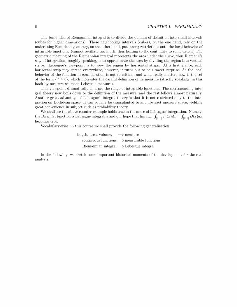
The basic idea of Riemannian integral is to divide the domain of definition into small intervals(cubes for higher dimensions). These neighboring intervals (cubes), on the one hand, rely on theunderlining Euclidean geometry, on the other hand, put strong restrictions onto the local behavior ofintegrable functions. (cannot oscillate too much, thus leading to the continuity to some extent) Thegeometric meaning of the Riemannian integral represents the area under the curve, thus Riemann’sway of integration, roughly speaking, is to approximate the area by dividing the region into verticalstrips. Lebesgue’s viewpoint is to view the region by horizontal strips. At a first glance, eachhorizontal strip may spread everywhere, however, it turns out to be a sweet surprise. As the localbehavior of the function in consideration is not so critical, and what really matters now is the setof the form f ≥ c, which motivates the careful definition of its measure (strictly speaking, in thisbook by measure we mean Lebesgue measure).
This viewpoint dramatically enlarges the range of integrable functions. The corresponding inte-gral theory now boils down to the definition of the measure, and the rest follows almost naturally.Another great advantage of Lebesgue’s integral theory is that it is not restricted only to the inte-gration on Euclidean space. It can equally be transplanted to any abstract measure space, yieldinggreat convenience in subject such as probability theory.
We shall see the above counter-example holds true in the sense of Lebesgue’ integration. Namely,the Dirichlet function is Lebesgue integrable and our hope that limn→∞
∫[0,1]
fn(x)dx =∫
[0,1]D(x)dx
becomes true.Vocabulary-wise, in this course we shall provide the following generalization:
length, area, volume, ... =⇒ measure
continuous functions =⇒ measurable functions
Riemannian integral =⇒ Lebesgue integral
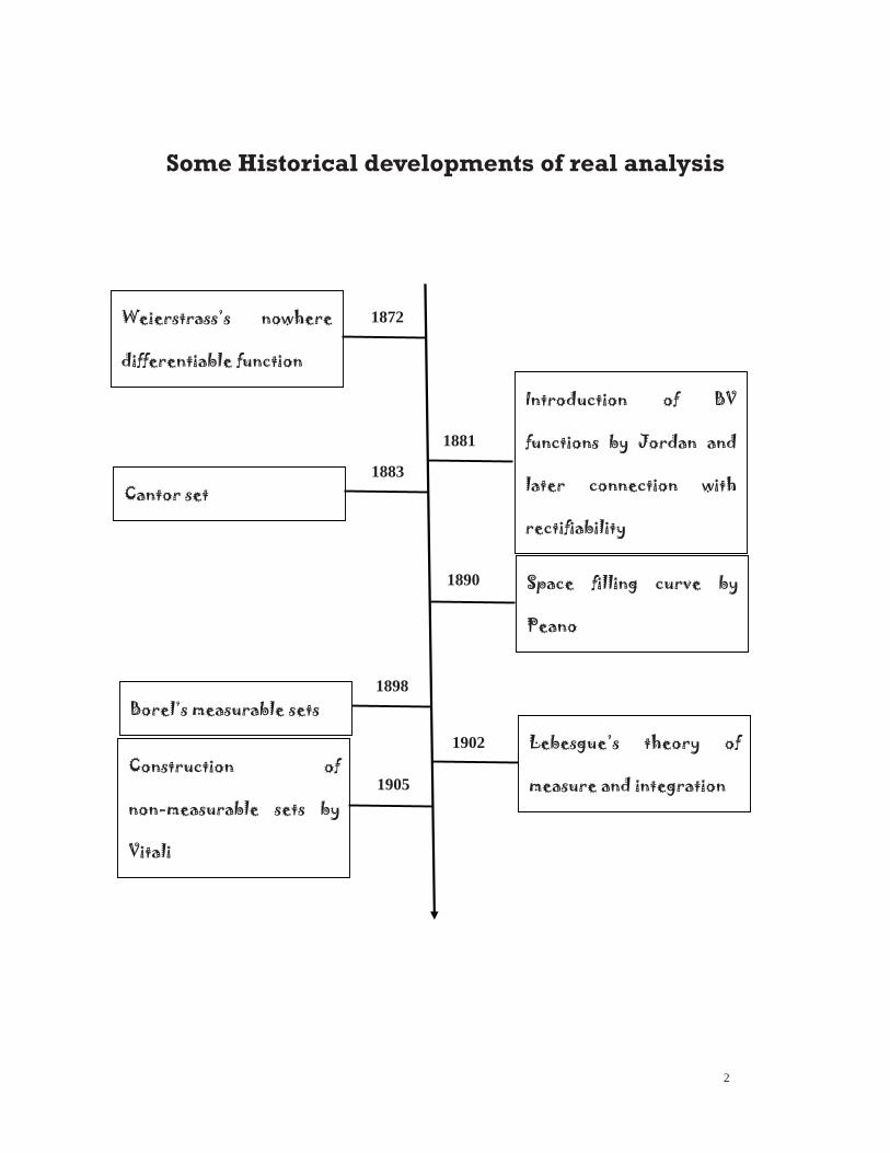
In the following, we sketch some important historical moments of the development for the realanalysis.
2
Some Historical developments of real analysis
Weierstrass’s nowhere
differentiable function
1872
Introduction of BV
functions by Jordan and
later connection with
rectifiability
Cantor set
Space filling curve by
Peano
Construction of
non-measurable sets by
Vitali
Borel’s measurable sets
Lebesgue’s theory of
measure and integration
1881
1883
1890
1898
1902
1905
8 CHAPTER 1. PRELIMINARY
The second part begins with the rudiment of the function spaces, followed by an introduction toFourier analysis. We study both Fourier series and Fourier transform together with their applications.The connection with real analysis is intimacy. There are also many unexpected connections of Fourieranalysis to wide-ranging mathematical topics such as Number theory, Discrete geometry, Probabilitytheory. We convey to the reader only a small portion of this fascinating subject.
1.2 Cardinality
In following sections, we establish some foundations on the set theory and the topology and geometryof the Euclidean space. We assume the reader is familiar with basic notions of sets, operationsbetween sets, etc. In this section, we address the following question: how to compare two sets withinfinite elements? This requires the concept of the cardinality of a set.
For two sets with finite number of elements, it is clear which set contains more elements. For twosets with infinite elements, which contains ’more’ elements relies on the mappings between them.
A map f : A → B is an assignment to each element of A a unique element in B. f is calledinjective, if f(x) 6= f(y), for x 6= y. f is called surjective if ∀z ∈ B, there exists x ∈ A such thatf(x) = z. A map f : A→ B is called a bijection if f is both injective and surjective. Clearly, a mapf : A→ B has a well-defined inverse, if and only if f is a bijection.
A and B are called to have same cardinality if there exists a bijection f : A → B, denoted byA ∼ B. Sometimes, we shall refer to the cardinal number of a set A, denoted by ¯A.
The cardinal number of natural numbers N is denoted by ℵ0. (Countable)
Example 1. Each infinite set contains a countable subset.
Example 2. Countable union of countable sets is countable.
Proof. Array this union as an infinite square, and enumerate in a zigzag way.
Example 3. All rational numbers Q is countable.
Example 4. Finite cartesian product of countable sets is countable.
Proof. Visualize this union as an infinite k dimensional cube, and enumerate in a zigzag way.
Example 5. The set of all real numbers R is not countable.
Proof. We prove (0, 1] is not countable. We accept each real number in (0, 1] has a decimal repre-sentation, which is unique if we don’t allow the appearance of all zeros after some position. That iswe write 0.25 as 0.249999999..., 1 as 0.99999...., etc.
Now suppose (0, 1] is countable, then we have an enumeration for all numbers in (0, 1], say0.a11a12a13...., 0.a21a22a23..., ... We can choose bii ∈ 0, 1, 2, ..., 9 \ aii, for each i. Let y =0.b11b22b33..., a moment of thought shows that y is indeed not in the enumeration list. A contradic-tion.
The cardinality of R is called ℵ1. The decimal representation shows that countable product offinite sets has cardinal number ℵ1.
Example 6. R, (0, 1], [0, 1], Rn all have same cardinal number ℵ1.
Theorem 1.1. There does not exist maximal cardinal number.
Proof. Given any set A, consider its power set 2A, namely the set of all subsets of A. We canshow they have different cardinality. Otherwise, there exists a bijection f : A → 2A, where f(a)corresponds to a subset of A. Define a subset of A as follows:
B = x|x /∈ f(x).

1.3. TOPOLOGY OF THE EUCLIDEAN SPACE 9
Now an amusing question confronts us: is B = f(x) for some x ∈ A?This proof is reminiscent of the barber paradox, which was raised by Bertrand Russell as follows:
a barber in a town claims to be the ”one who shaves all those, and those only, who do not shavethemselves.” The question is, does the barber shave himself?
Remark 1.2 (Continuum hypothesis). Cantor in 1878 raised the following hypothesis concerning thesize of infinite sets:
There is no set whose cardinality is strictly between that of the integers and the real numbers.
Establishing its truth or falsehood is the first of Hilbert’s 23 problems presented in 1900. The readeris referred to https://en.wikipedia.org/wiki/Continuum hypothesis for a thorough introduction.
1.3 Topology of the Euclidean space
We use Rn for n-dimensional Euclidean space. For x = (x1, · · · , xn and y = (y1, · · · , yn), the innerproduct is defined as
x · y = x1y1 + x2y2 + · · ·+ xnyn.
Norm is defined as
|x| =√x2
1 + · · ·+ x2n.
Open ball centered at x of radius r is denoted by B(x, r), i.e.,
B(x, r) = y||y − x| < r.
Closed ball is B(x, r) = y||y − x| ≤ r.An open cube is of the form (a1, b1)×(a2, b2)×· · ·×(an, bn), closed cube is [a1, b1]×· · ·× [an, bn].
A half-open half-closed cube is of the form (a1, b1]× · · · × (an, bn].Given A ⊂ Rn, x is called an interior point of A if there exists r > 0 such that B(x, r) ⊂ A. A
is called an open set, if every point of A is an interior point. x is called an accumulation point of A,if (B(x, r) \ x) ∩ A 6= ∅, for all r > 0. The union of A with its accumulation points is called theclosure of A, denoted by A. A set A is called closed, if A is an open set.
A family of open sets Oαα∈Λ is called an open cover of A if A ⊂⋃αOα. A is bounded if there
exists R > 0, such that A ⊂ B(0, R). A set is called compact if it is both bounded and closed. Anice property of being a compact set is that any open cover has a finite subcover.
Theorem 1.3 (Heine-Borel). A ⊂ Rn is a compact set if and only if every open cover of A containsa finite subcover.
We also recall the theorem of nested closed sets.
Theorem 1.4. Let A1 ⊃ A2 ⊃ · · · ⊃ An ⊃ · · · be a sequence of nested non-empty closed sets. Then⋂∞n=1An 6= ∅.B ⊂ A is called dense in A, if B = A. A is called nowhere dense if there exists no interior point
of A.
Example 7. Take r /∈ Q, < x > denotes the fractional part of x. Then < rn >n=1,2,··· is dense in[0, 1].
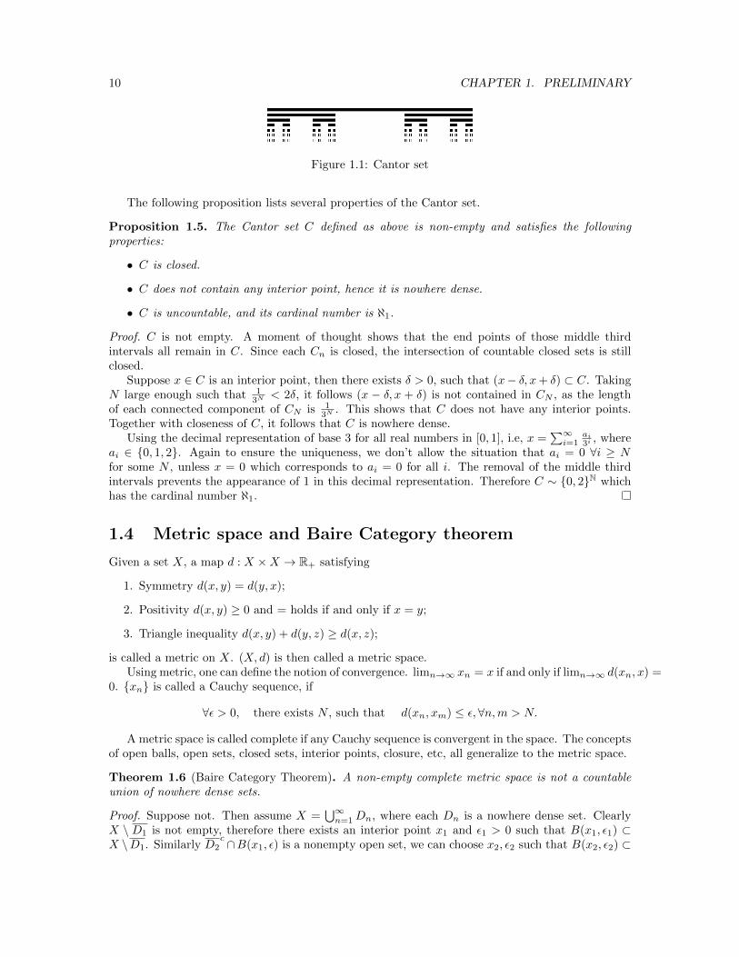
Example 8 (Cantor set). Let C0 = [0, 1] the unit closed interval. C1 = [0, 13 ] ∪ [ 2
3 , 1], the removal ofthe middle 1
3 open interval from C0. Cn is obtained inductively by removing the middle one thirdopen intervals of each connected components of Cn−1. For example, C2 = [0, 1
9 ]∪[ 29 ,
13 ]∪[ 2
3 ,79 ]∪[ 8
9 , 1].
C :=
∞⋂n=0
Cn
is the Cantor set.
10 CHAPTER 1. PRELIMINARY
Figure 1.1: Cantor set
The following proposition lists several properties of the Cantor set.
Proposition 1.5. The Cantor set C defined as above is non-empty and satisfies the followingproperties:
• C is closed.
• C does not contain any interior point, hence it is nowhere dense.
• C is uncountable, and its cardinal number is ℵ1.
Proof. C is not empty. A moment of thought shows that the end points of those middle thirdintervals all remain in C. Since each Cn is closed, the intersection of countable closed sets is stillclosed.
Suppose x ∈ C is an interior point, then there exists δ > 0, such that (x− δ, x+ δ) ⊂ C. TakingN large enough such that 1
3N< 2δ, it follows (x − δ, x + δ) is not contained in CN , as the length
of each connected component of CN is 13N
. This shows that C does not have any interior points.Together with closeness of C, it follows that C is nowhere dense.
Using the decimal representation of base 3 for all real numbers in [0, 1], i.e, x =∑∞i=1
ai3i , where
ai ∈ 0, 1, 2. Again to ensure the uniqueness, we don’t allow the situation that ai = 0 ∀i ≥ Nfor some N , unless x = 0 which corresponds to ai = 0 for all i. The removal of the middle thirdintervals prevents the appearance of 1 in this decimal representation. Therefore C ∼ 0, 2N whichhas the cardinal number ℵ1.
1.4 Metric space and Baire Category theorem
Given a set X, a map d : X ×X → R+ satisfying
1. Symmetry d(x, y) = d(y, x);
2. Positivity d(x, y) ≥ 0 and = holds if and only if x = y;
3. Triangle inequality d(x, y) + d(y, z) ≥ d(x, z);
is called a metric on X. (X, d) is then called a metric space.Using metric, one can define the notion of convergence. limn→∞ xn = x if and only if limn→∞ d(xn, x) =
0. xn is called a Cauchy sequence, if
∀ε > 0, there exists N , such that d(xn, xm) ≤ ε,∀n,m > N.
A metric space is called complete if any Cauchy sequence is convergent in the space. The conceptsof open balls, open sets, closed sets, interior points, closure, etc, all generalize to the metric space.
Theorem 1.6 (Baire Category Theorem). A non-empty complete metric space is not a countableunion of nowhere dense sets.
Proof. Suppose not. Then assume X =⋃∞n=1Dn, where each Dn is a nowhere dense set. Clearly
X \ D1 is not empty, therefore there exists an interior point x1 and ε1 > 0 such that B(x1, ε1) ⊂X \D1. Similarly D2
c ∩B(x1, ε) is a nonempty open set, we can choose x2, ε2 such that B(x2, ε2) ⊂
1.5. CONTINUOUS FUNCTIONS AND DISTANCE IN METRIC SPACE 11
D2c ∩B(x1, ε). Inductively, we get a sequence of nested balls B(xn, εn) ⊂ B(xn−1, εn−1), moreover
we can easily arrange that limn→∞ εn = 0. Thus xn is a Cauchy sequences and it converges to,say x. Since X =
⋃∞n=1Dn, thus x ∈ Dk for some k. However due to the construction x ∈ B(xk, εk),
which contradicts to that B(xk, εk) ∩Dk = ∅.
Using the Baire category theorem, we get another proof that [0, 1] is uncountable.Countable intersection of open sets is called a Gδ set, countable union of closed sets is called an
Fσ set. We give a more interesting application of Baire’s category theorem.
Proposition 1.7. There does not exist a function f : R→ R which is continuous only at all rationalnumbers.
We need a lemma first.
Lemma 1.8. The points of continuity of f is a Gδ set.
Proof. Recall that f is continuous at x if and only if the oscillation ωf (x) = 0. Therefore the set ofpoints of continuity of f is
∞⋂n=1
x|ωf (x) <1
n.
It is easy to show that x|ωf (x) < 1n is open.
Proof of the Proposition. Using the above lemma, it is suffice to show that Q is not a Gδ set. Supposenot, then assume
Q =
∞⋂n=1
Gn,
where each Gn is open set. We write Q as Q = q1, q2, · · · , then
R =
∞⋃n=1
Gcn
∞⋃i=1
qi.
Gcn is closed, suppose it contains an interior point, then there exists an open interval (x, y) ⊂ Gcn.Therefore
(x, y)c ⊃ Gn ⊃ Q.
The only possible case is x = y. Hence Gcn is nowhere dense.The above expression writes R as a union of countable nowhere dense sets. This contradicts to
the Baire category theorem.
1.5 Continuous functions and Distance in metric space
Given a function f : E ⊂ Rn → R, f is continuous at x ∈ E, if ∀ε > 0, there exists δ > 0 such that
|f(y)− f(x)| ≤ ε, ∀y ∈ B(x, δ) ∩ E.
f is called continuous on E if f is continuous at every point of E. This definition does not requireE is open.
Theorem 1.9. Suppose f : F → R be a continuous function defined on a compact set F , then f isuniform continuous and attains its maximum and minimum.
12 CHAPTER 1. PRELIMINARY
The limit of a sequence of continuous functions which converges uniformly is continuous.A natural and useful function on the Euclidean space is the distance function. Given E ⊂ Rn,
let
d(x,E) = infy∈E
d(x, y).
By triangle inequality, it is easy to see that d(x,E) is Lipschitz continuous, and thus uniformlycontinuous.
We aim to prove the following Tietze extension theorem in Rn. It actually holds in more generalmetric space, we leave the exploration to interested readers.
Theorem 1.10 (Tietze extension). Let f : E → R be a continuous function defined on a closed setE ⊂ Rn with |f(x)| ≤ C, then there exists a continuous function F : Rn → R satisfying
F |E = f and |F (x)| ≤ C.
Proof. Set
A := f−1([−C,−C3
]) B := f−1([−C3,C
3]) C := f−1([
C
3, C]).
Since A and C are two disjoint closed sets, the function
g1(x) :=C
3
d(x,A)− d(x,C)
d(x,A) + d(x,C),
is well-defined. It is easy to see that
|g1(x)| ≤ C
3∀x ∈ Rn
and
|f(x)− g1(x)| ≤ 2C
3∀x ∈ E.
Repeat the same process for |f − g1| with the bound being 2C3 , we get
|g2(x)| ≤ 2C
9and |f − g1 − g2| ≤
4C
9.
Inductively, we get a sequence of continuous function gn(x) defined on Rn satisfying
|gn(x)| ≤ 2n−1C
3nand |f − (
n∑i=1
gi)| ≤2nC
3n.
The former implies that gn(x) converges uniformly to a continuous function, say G(x) with
|G(x)| ≤ C;
the latter implies |f(x)−G(x)| = 0 for x ∈ E.
Remark 1.11. The point of Tietze extension theorem is that f is defined on a close set. It is notalways possible to extend a continuous function defined on an open interval. A simple example isf(x) = sin( 1
x ), x ∈ (0, 1].
Remark 1.12. A continuous function defined on a closed set needs not to be bounded, howevercontinuous extension still exits.
1.5. CONTINUOUS FUNCTIONS AND DISTANCE IN METRIC SPACE 13
1.5.1 Hausdorff distance and Gromov-Hausdorff distance
Let X be a subset of a metric space, its ε-neighborhood is defined as
Xε = ∪x∈Xy|d(x, y) ≤ ε.
The Hausdorff distance between two subsets X,Y is defined as
dH(X,Y ) = infε ≥ 0|X ⊂ Yε, Y ⊂ Xε.
It is a pseudometric on all subsets, because dH(X,Y ) = 0 does not necessarily mean X = Y . Whenrestricting to closed subsets,dH(·, ·) becomes a metric. To avoid dH(X,Y ) = ∞, we work furtherwith compact subsets.
Theorem 1.13. Let (X , d) be a metric space. Denote by D(X ) the collection of compact subsets ofX . Then we have following
• The Hausdorff distance dH(·, ·) defines a metric on D(X ).
• (D(X ), dH(·, ·)) is compact if X is compact.
• (D(X ), dH(·, ·)) is complete if X is complete.
Proof. To show dH(·, ·) defines a metric on D(X ), we need to show
1. Triangle inequality: dH(X,Y ) ≤ dH(X,Z) + dH(Z, Y ).
2. dH(X,Y ) = 0 if and only if X = Y .
Proof of 1 Assume dH(X,Z) = r and dH(Z, Y ) = s, for r1 > r and s1 > s, we have Z ⊂ Ys1 andX ⊂ Zr1 , which implies
X ⊂ Zr1 ⊂ Yr1+s1 .
Similarly, Z ⊂ Xr1 and Y ⊂ Zs1 , which implies
Y ⊂ Zs1 ⊂ Xr1+s1 .
Together we obtain dH(X,Y ) ≤ r1 + s1, since r1 and s1 are arbitrary, the proof is finished.proof of 2 Suppose there exists x ∈ X but x /∈ Y , then d(x, Y ) = δ > 0. Moreover, since Y is a
compact, there exists y ∈ Y such that d(x, y) = d(x, Y ). Hence X * Yr for r < δ. This contradictsto dH(X,Y ) = 0. Thus X ⊂ Y , likewise we have Y ⊂ X. Thus the conclusion follows.
We leave the rest of proof to the reader.
Hausdorff distance measures the closeness of two subsets of a given metric space. Gromov-Hausdorff distance extends this idea to an intrinsic way of measuring distance between two arbitrarymetric spaces. The idea is to allow isometric motion in an ambient metric space. i : X → Y is calledan isometric embedding of (X, dX) into (Y, dY ), if dX(p, q) = dY (i(p), i(q)), ∀p, q ∈ X. Given twometric spaces X,Y , the Gromov-Hausdorff distance is defined as
dGH(X,Y ) = infdH(i(X), j(Y )),
where the inf is taken over all metric spaces Z and isometric embeddings i : X → Z and j : Y → Z.
Theorem 1.14. dGH defines a metric on the space of compact metric spaces modulo isometries.
We state another convenient description of Gromov-Hausdorff distance. A map f : X → Y iscalled an ε-isometry, if
14 CHAPTER 1. PRELIMINARY
• |dX(x, x′)− dY (f(x), f(x′)| ≤ ε, ∀x, x′ ∈ X;
• f(X) is an ε-net of Y .
A subset Z ⊂ X is an ε-net if Zε ⊃ X.
Proposition 1.15. • dGH(X,Y ) < ε⇒ ∃f : X → Y a 2ε-isometry;
• ∃f : X → Y an ε-isometry ⇒ dGH(X,Y ) < 2ε.
Proof of Theorem 1.14. The nontrivial part is to show dGH(X,Y ) = 0 if and only if X is isometricto Y . One direction is easy. We just need to show the other direction that dGH(X,Y ) = 0 impliesthat X is isometric to Y . To this end, we first extract a countable dense subset S of X. Thiscan be done as follows. Since X is compact, there exists a finite set of X which forms a 1
n -net forX. The countable union of these 1
n -net is a countable dense subset of X, denoted by S. AssumeS = s1, s2, · · · . By Proposition 1.15, there exists 1
n -isometry fn : X → Y . Since fn(s1)∞n=1
is a sequence in a compact set Y , thus we can take a convergent subsequence. Now for s2, we cantake a convergent sub-subsequence. Inductively, we find a subsequence of fn (still denoted by fn forsimplicity), which converges at each point of S. Suppose the limit function is f . Hence
|dX(s, s′)− dY (f(s), f(s′))| = limn→∞
|dX(s, s′)− dY (fn(s), fn(s′))| = 0, ∀s, s′ ∈ X,
which means f preserves metric on S. Since S is a dense subset of X, f has a unique continuousextension f , which also preserves the metric. Working in the other direction, we get a metricpreserving map g : Y → X. Thus X is isometric to Y .
1.5.2 Invariant of domain
From set theoretical point view, Rn and Rm have same cardinality. However, the one-to-one corre-spondence is not easy to write down. When taking more structure into consideration, Rn and Rmare distinct. For example, there does not exist continuous one-to-one correspondence. This is theinvariance of domain and relates the notion of topological dimension.
Theorem 1.16 (Invariance of domain). Let U ⊂ Rn be an open set and f : U → Rn is injectiveand continuous, then f(U) is also open in Rn.
Corollary 1.17. Rn is not homeomorphic to Rm, for n 6= m.
f : X → Y between two metric spaces is called a homeomorphism if it is
• injective and surjective,
• continuous,
• its inverse is also continuous.
Proof. Suppose n < m and let f : Rm → Rn be the homeomorphism. Then by adding m− n zeros,i.e F (x) = (f(x), 0, · · · , 0), we get an injective continuous map from Rm to Rn, whose image fails tobe an open set. A contradiction to invariance of domain.
We can also rephrase the proof to the following fact
Theorem 1.18. There does not exist a continuous injection from Rn to Rm for n > m.
The converse direction is
Theorem 1.19. There exists a continuous surjection from Rn to Rm for n < m.
1.5. CONTINUOUS FUNCTIONS AND DISTANCE IN METRIC SPACE 15
The famous Peano curve provides such an example.When adding the linear structure into account, we come to the more familiar facts from linear
algebra.
Proposition 1.20. There does not exist a linear injection from Rn to Rm for n > m.
Proposition 1.21. There does not exist a linear surjection from from Rn to Rm for n < m.

16 CHAPTER 1. PRELIMINARY
Chapter 2
Lebesgue measure
11§!ËÆØ£Up§/þ))oå5£¼á6
In this chapter, we shall generalize ’length, area, volume, ...’ of regular regions to the measure ofarbitrary sets. There are two steps involved. The idea of the first step is to approximate a general setby familiar regular sets: open cubes. However, this approximation is more plausible from exterior ofa set, which leads to the definition of the exterior measure. The second step is the discovery that toencompass the property of the disjoint additivity, one has to disregard some sets of highly irregular(non-measurable sets). Therefore a satisfactory measure theory does not include all subsets of Rn.
2.1 Exterior measure
As said above, measure is a generalization of ’length, area, volume, ...’ . So the very first agreementis that the measure of the n-dimensional open cube C = (a1, b1) × · · · (an, bn) is its volume (b1 −a1)× · · · (bn − an), and measure of regular regions are their volume. Moreover, geometric intuitionechoes that any such generalization should inherit nice properties of volume, such as
• monotone: if A ⊂ B, then A’s measure is not greater than B’s measure;
• disjoint additivity: ∪ni=1Ai’s measure is the sum of Ai’ measure if Ai are disjoint;
• translation invariant;
• Scaling property.
We use the covering of cubes to define the measure for a general set, and we shall allow countablemany cubes for the covering.
Definition 2.1. Given E ⊂ Rn, the exterior measure of E is defined as
m∗(E) := infE⊂∪∞k=1Ik
∞∑k=1
|Ik|,
where Ik∞k=1 is a sequence of countable open cubes that cover E and |Ik| is the volume of Ik.
17
18 CHAPTER 2. LEBESGUE MEASURE
The reason we call it exterior measure rather than measure will be clear momentarily. Before thatwe shall get used to this definition by exploring several simple yet important facts and properties ofthe exterior measure.
Example 9. Let A be a set consists of countable many points, then m∗(A) = 0.
Proof. This proof is a common trick in real analysis, which relies on
∞∑n=1
ε
2n= ε.
Example 10. m∗(C) = 0, where C is the Cantor set.
Remark 2.2. The definition builds on the volume of n-dimensional cubes. Therefore it can’t distin-guish sets of ’lower dimension’. For example, a line segment in R2 has exterior measure (area) zero,but it certainly has length. The more intrinsic way to encode the dimension information of sets isthe notion called Hausdorff measure.
The next theorem shows that the exterior measure has all the nice properties we could expect.
Theorem 2.3. The exterior measure satisfies the following
• nonnegativity: m∗(E) ≥ 0;
• monotone: if A ⊂ B, then m∗(A) ≤ m∗(B);
• sub-additivity: m∗(∪∞k=1Ak) ≤∑∞k=1m
∗(Ak);
• translation invariant: m∗(E + x0) = m∗(E);
• scaling: m∗(λE) = λnm∗(E); ∀λ > 0.
Proof. We only prove the sub-additivity. The rests follow more or less directly from definition andthus are left to the reader. ∀ε > 0, there exists a covering of open cubes Ik,i for each Ak, suchthat
m∗(Ak) ≤∞∑i=1
|Ik,i| < m∗(Ak) +ε
2k.
Clearly ∪∞i,k=1Ii,k is a countable union of open cubes that covers ∪∞k=1Ak, thus
m∗(∪∞k=1Ak) ≤∞∑k=1
∞∑i=1
|Ik,i| <∞∑k=1
m∗(Ak) + ε.
Since ε is arbitrary, we get the desired sub-additivity.
There is still one unsatisfied issue: the exterior measure only has subadditivity, and is lack ofadditivity for disjoint sets. That is
m∗(∪∞k=1Ak) =
∞∑k=1
m∗(Ak)
whenever Ak are disjoint. Here is an example.
2.2. MEASURE 19
Example 11. [A non-measurable set] We shall construct a set N ⊂ [0, 1]. First, we define anequivalent relation, say x ∼ y if x − y ∈ Q. Under this equivalent relation, [0, 1] can be written asthe disjoint union of different equivalent classes:
[0, 1] =⋃α∈Λ
Eα.
We pick a representative rα ∈ Eα in each equivalent class and set N := rαα∈Λ.Denote all rational numbers in [−1, 1] as q1, q2, · · · , . We claim Nk := N + qk are disjoint.
Suppose Nk ∩ Nl 6= ∅, then there exists x, y ∈ N , such that x + qk = y + ql, which means x ∼ y.This contradicts the only one pick from each equivalent class.
If Nk satisfied the disjoint additivity, we would have
m∗(
∞⋃k=1
Nk) =
∞∑k=1
m∗(Nk).
Clearly,
[0, 1] ⊂∞⋃k=1
Nk ⊂ [−1, 2],
and thus
1 ≤∞∑k=1
m∗(Nk) ≤ 3. (2.1)
In view of the translation invariant, m∗(Nk) = m∗(N),∀k. No value for m∗(N) would justify (2.1).
Remark 2.4. We shall point out, the definition of N , namely the pick of one element from eachequivalent class requires the Axiom of choice. Formally, it states that for every indexed family(Si)i∈I of nonempty sets there exists an indexed family (xi)i∈I of elements such that xi ∈ Sifor every i ∈ I. The reader is referred to https://en.wikipedia.org/wiki/Axiom of choice for moredetails.
2.2 Measure
The example 11 shows in general we do not have disjoint additivity of exterior measure for all subsetsof Rn. A remedy is to restrict our attention to those sets, for which the disjoint additivity hold.
Caratheodory made the following convenient criterion for the sets we shall be concerned with.
Definition 2.5. Let A ⊂ Rn, A is called a measurable set if
m∗(T ) = m∗(T ∩A) +m∗(T ∩Ac), ∀T ⊂ Rn. (2.2)
A useful observation is that to verify (2.2), one just needs to showm∗(T ) ≥ m∗(T∩A)+m∗(T∩Ac)Since m∗(T ) ≤ m∗(T ∩A) +m∗(T ∩Ac) always holds by the sub-additivity.
Suppose m∗(A) = 0, then m∗(T ∩ A) = 0 and m∗(T ∩ Ac) ≤ m∗(T ), we infer that all sets withzero exterior measure are measurable.
The collection of all measurable sets is denoted by M. We prove the following
Theorem 2.6. 1. ∅ ∈ M;
2. if A ∈M, then Ac ∈M;
20 CHAPTER 2. LEBESGUE MEASURE
3. if Ak ∈M for k = 1, 2, · · · , then ∪∞k=1Ak ∈M, moreover
m∗(∪∞k=1Ak) =
∞∑k=1
m∗(Ak)
whenever Ak are disjoint.
Proof. Notice (2.2) is symmetric about A and Ac, 2 of the theorem immediately follows. To show 3,we first show if A1, A2 ∈M, then A1 ∪A2 ∈M. Using A1, A2 are measurable, we have for any T ,
m∗(T ) = m∗(T ∩A1) +m∗(T ∩Ac1)
= m∗(T ∩A1 ∩A2) +m∗(T ∩A1 ∩Ac2) +m∗(T ∩Ac1 ∩A2) +m∗(T ∩Ac1 ∩Ac2).
Notice T ∩ (A1 ∪A2) = (T ∩A1 ∩A2)∪ (T ∩A1 ∩Ac2)∪ (T ∩Ac1 ∩A2), by sub-additivity, we have
m∗(T ∩ (A1 ∪A2)) ≤ m∗(T ∩A1 ∩A2) +m∗(T ∩A1 ∩Ac2) +m∗(T ∩Ac1 ∩A2),
and thus
m∗(T ) ≥ m∗(T ∩ (A1 ∪A2)) +m∗(T ∩Ac1 ∩Ac2) = m∗(T ∩ (A1 ∪A2)) +m∗(T ∩ (A1 ∪A2)c).
This implies that A1 ∪A2 ∈M.Moreover suppose A1 ∩A2 = ∅, then setting T = A1 ∪A2 in m∗(T ) = m∗(T ∩A1) +m∗(T ∩Ac1),
we get the additivity for two disjoint sets:
m∗(A1 ∪A2) = m∗(A1) +m∗(A2). (2.3)
Setting T of the form T ∩ (A1 ∪A2) we also have
m∗(T ∩ (A1 ∪A2)) = m∗(T ∩A1) +m∗(T ∩A2). (2.4)
Iterate this process finite many times together with the property 2, we infer that if A1, · · ·An ∈M, then any union or intersection among them is still measurable, and finite disjoint additivityholds, i.e.,
m∗(∪ni=1Ai) =
n∑i=1
m∗(Ai),
and
m∗(T ∩ (∪ni=1Ai)) =
n∑i=1
m∗(T ∩Ai),
whenever Ai are all disjoint.For countable union, first suppose A1, · · · , An, · · · ∈ M are all disjoint. Let S := ∪∞n=1An and
Sk = ∪kn=1An. Using Sk ∈M, we have for any T that
m∗(T ) = m∗(T ∩ Sk) +m∗(T ∩ Skc)
=
k∑n=1
m∗(T ∩An) +m∗(T ∩ Skc) ≥
k∑n=1
m∗(T ∩An) +m∗(T ∩ Sc).
Above inequality holds for all k, letting k →∞ we obtain
m∗(T ) ≥∞∑n=1
m∗(T ∩An) +m∗(T ∩ Sc) ≥ m∗(T ∩ S) +m∗(T ∩ Sc).
2.2. MEASURE 21
Hence S ∈M.Using T ∩ S in the above inequality, we get
m∗(T ∩ S) ≥∞∑n=1
m∗(T ∩An).
On the other hand, m∗(T ∩ S) ≤∑∞n=1m
∗(T ∩An) always holds by sub-additivity. Therefore
m∗(T ∩ S) =
∞∑n=1
m∗(T ∩An),
by taking T = Rn, we get the disjoint additivity.Finally, if An ∈ M are not necessarily disjoint from each other, then we make the following
change:B1 = A1, Bk = (∪ki=1Ai) \ ((∪k−1
i=1 Ai)) ∀k ≥ 2.
It follows Bk are disjoint and ∪∞n=1An = ∪∞k=1Bk ∈M.
From now on we shall write simply m(A) for the exterior measure of a measurable set A. Ourtask of defining the measure for suitable subsets of Rn is now completed.
We conclude this section with two useful facts about interchanging measure with limit operation.
Proposition 2.7. Let An ⊂ An+1 be a sequence of increasing measurable sets, set A = ∪nAn, then
m(A) = limn→∞
m(An).
Proof. If m(An) =∞ for some n, then the desired equality holds. Therefore we assume m(An) <∞for all n. Set B1 = A1, B2 = A2 \ A1, Bn = An \ An−1, then Bn are all disjoint. Using countabledisjoint additivity, we get
m(∪nBn) =
∞∑k=1
m(Bk).
We obtain the desired equality as ∪nBn = ∪nAn and m(An) =∑nk=1m(Bk).
For decreasing sequence, we have
Proposition 2.8. Let An ⊃ An+1 be a sequence of decreasing measurable sets, set A = ∩nAn,assume m(A1) <∞ then
m(A) = limn→∞
m(An). (2.5)
Proof. We view A1 as the ambient set and take complement with respect to A1. We then have
∅ ⊂ Ac2 ⊂ · · · ⊂ Acn · · · ,
Applying Proposition 2.7, we have
m(∪nAcn) = limn→∞
m(Acn). (2.6)
Sincem(Acn) +m(An) = m(A1) and m(∪nAcn) +m(A) = m(A1),
plugging back to (2.6), we get (2.5).
Remark 2.9. The assumption m(A1) <∞ is necessary. For example, let An = (n,∞), then ∩nAn =∅ and (2.5) fails.
22 CHAPTER 2. LEBESGUE MEASURE
2.3 Borel sets and Measurable sets
In this section, we explore some relation between measurable sets and open, closed sets. Thefirst question we should answer is whether open cubes are measurable? The answer is definitelyaffirmative:
Theorem 2.10. If G is an open set, then G is measurable.
We need two lemmas. First recall two definitions. The distance between a point and a set isdefined as
d(x,A) = infy∈A
d(x, y),
and the distance between two sets is defined as
d(A1, A2) = infx∈A1,y∈A2
d(x, y).
Lemma 2.11. Let A1, A2 be two sets with d(A1, A2) > 0, then
m∗(A1 ∪A2) = m∗(A1) +m∗(A2).
Proof. Observe first that in the definition of the exterior measure, we could require the side lengthesof all open cubes are ≤ δ for a fixed δ > 0. To prove the lemma, we just need to show m∗(A1∪A2) ≥m∗(A1) +m∗(A2). Suppose d(A1, A2) = 2δ > 0, then for any ε > 0, there exit countable open cubesDi of side lengthes ≤ δ covering A1 ∪A2 such that
m∗(A1 ∪A2) + ε ≥∞∑i=1
|Di|.
We can divide Di into two groups D(1)j and D(2)
j such that
∪∞j=1D(1)j ⊃ A1 and ∪∞j=1 D
(2)j ⊃ A2.
Since d(A1, A2) = 2δ > 0, all side lengthes ≤ δ, it follows that D(1)k ∩D
(2)l = ∅, ∀k, l. Hence
m∗(A1 ∪A2) + ε ≥∞∑i=1
|Di| =∞∑j=1
|D(1)j |+
∞∑j=1
|D(2)j | ≥ m
∗(A1) +m∗(A2).
Since ε is arbitrary, we get the desired inequality.
Lemma 2.12 (Caratheodory). Suppose G 6= Rn is an open set, E ⊂ G, let
Ek = x ∈ E : d(x,Gc) ≥ 1
k, k = 1, 2, · · · ,
then limk→∞
m∗(Ek) = m∗(E).
Proof. Clearly, Ek ⊂ Ek+1 ⊂ E and ∪∞k=1Ek = E, it follows that m∗(Ek) is monotone increasingand limk→∞m∗(Ek) ≤ m∗(E).
It remains to show that m∗(E) ≤ limk→∞m∗(Ek). It suffices to assume limk→∞m∗(Ek) < ∞.Let Ak = Ek \ Ek−1, then d(Ak, Ak+2) > 0. Note
m∗(E2k) ≥ m∗(∪ki=1A2i) =
k∑i=1
m∗(A2i).
2.3. BOREL SETS AND MEASURABLE SETS 23
The equality is due to Lemma 2.11. In view of the assumption limk→∞m∗(Ek) <∞,∑∞i=1m
∗(A2i)
is convergent. Similarly,∑ki=1m
∗(A2i−1) is also convergent.Since E = E2k ∪ (∪j>kA2j) ∪ (∪j>kA2j−1), by sub-additivity, we have
m∗(E) ≤ m∗(E2k) +m∗(∪j>kA2j) +m∗(∪j>kA2j−1)
≤ m∗(E2k) +∑j>k
m∗(A2j) +∑j>k
m∗(A2j−1).
Letting k →∞, we obtain that m∗(E) ≤ limk→∞m∗(E2k). This completes the proof.
Proof of Theorem 2.10. We just need to show
m∗(T ) ≥ m∗(T ∩G) +m∗(T ∩Gc), ∀T ⊂ Rn.
By Lemma 2.12, there exist sets Tk ⊂ T ∩G, such that
limk→∞
m∗(Tk) = m∗(T ∩G).
Sincem∗(T ) ≥ m∗(Tk) +m∗(T ∩Gc),
letting k →∞, we get the desired inequality.
Definition 2.13. A collection T of subsets of X satisfying
• ∅ ∈ T ;
• if A ∈ T , then Ac ∈ T ;
• if Ak ∈ T for k = 1, 2, · · · , then ∪∞k=1Ak ∈ T ;
is called a σ-algebra.
Given a collection Γ of subsets of X, the minimal σ-algebra containing Γ is called the σ-algebragenerated by Γ. In Rn, the σ-algebra generated by all open sets is called the Borel algebra, denotedby B. Its element is called a Borel set. Therefore, all closed sets, Gδ sets, Fσ sets, and their countableunions, etc, are all Borel sets.
Then a direct consequence of Theorem 2.10 is
Corollary 2.14. All Borel sets are measurable.
Finally we show up to a set of measure zero, a measurable set is either a Gδ or an Fσ set.
Proposition 2.15. Let A be a measurable set, then ∀ε > 0,
• there exists an open set G ⊃ A, such that m(G \A) < ε;
• there exists a closed set F ⊂ A, such that m(A \ F ) < ε.
Proof. First assume m(A) <∞. Then ∀ε > 0, there exists countable open cubes Di covering A suchthat
∞∑i=1
|Di| < m(A) + ε.
Let G = ∪∞i=1Di which is an open set containing A. Since A is measurable, we have
m(G \A) = m(G)−m(A) ≤∞∑i=1
|Di| −m(A) < ε.

24 CHAPTER 2. LEBESGUE MEASURE
For m(A) = ∞, we let An := A ∩ B(0, n). For fixed ε > 0 and n, there exists an open setGn ⊃ An, such that
m(Gn \An) <ε
2n.
Let G = ∪nGn, it follows that G ⊃ A is an open set and
m(G \A) ≤∞∑n=1
m(Gn \An) ≤ ε.
The second statement can be obtained dually by the De Morgan’s law.
Remark 2.16. Instead of the Caratheodory criterion, one can use the first statement of the Propo-sition to define measurable set. The reader is referred to Stein’s book for this treatment.
Proposition 2.17. Let A be a measurable set, then
• there exists a Gδ set G ⊃ A, such that m(G \A) = 0;
• there exists an Fσ set F ⊂ A, such that m(A \ F ) = 0.
Proof. By Proposition 2.15, for ε = 1n , there exists an open set Gn ⊃ A such that
m(Gn \A) <1
n.
Let G = ∩∞n=1Gn, it follows that G ⊃ A and
m(G \A) ≤ m(Gn \A) <1
n, ∀n.
Hence m(G \A) = 0. The second statement follows similarly.
2.4 Linear transformation of measurable sets
In this section, we briefly discuss how to obtain classical area formula for triangle and disk in ameasure theoretical way. What we use are the properties of measure and the transformation law ofmeasure of a set under linear transformations. The latter can be viewed as the change of variableformula in multi-variable Calculus.
Theorem 2.18. Let T : Rn → Rn be a non-singular linear transformation, then for any measurableset A,
m(T (A)) = |det(T )|m(A). (2.7)
Proof. The proof is divided into two steps.Step 1: reduction of A to unit cubeFrom Proposition 2.17, a general measurable set A differs from a Gδ set AG by a set of measurezero, and any open set is countable union of open cubes. Therefore it suffices to verify (2.7) for unitcube D0.
Step 2: decomposition of a linear transformation into following three simple transformations:
1. T (xi) = xj , T (xj) = xi, T (xk) = xk for k 6= i, j;
2. T (x1) = λx1, T (xi) = xi for i ≥ 2 and λ 6= 0;
2.5. SETS OF POSITIVE MEASURE 25
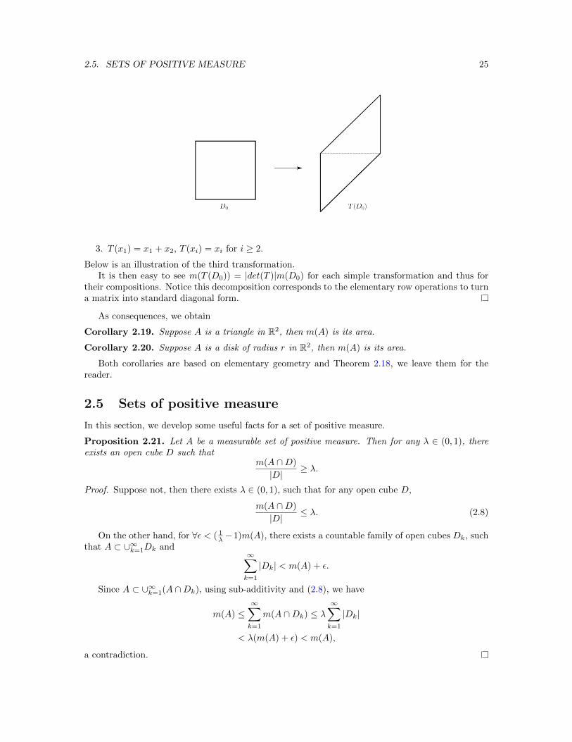
3. T (x1) = x1 + x2, T (xi) = xi for i ≥ 2.
Below is an illustration of the third transformation.It is then easy to see m(T (D0)) = |det(T )|m(D0) for each simple transformation and thus for
their compositions. Notice this decomposition corresponds to the elementary row operations to turna matrix into standard diagonal form.
As consequences, we obtain
Corollary 2.19. Suppose A is a triangle in R2, then m(A) is its area.
Corollary 2.20. Suppose A is a disk of radius r in R2, then m(A) is its area.
Both corollaries are based on elementary geometry and Theorem 2.18, we leave them for thereader.
2.5 Sets of positive measure
In this section, we develop some useful facts for a set of positive measure.
Proposition 2.21. Let A be a measurable set of positive measure. Then for any λ ∈ (0, 1), thereexists an open cube D such that
m(A ∩D)
|D|≥ λ.
Proof. Suppose not, then there exists λ ∈ (0, 1), such that for any open cube D,
m(A ∩D)
|D|≤ λ. (2.8)
On the other hand, for ∀ε < ( 1λ −1)m(A), there exists a countable family of open cubes Dk, such
that A ⊂ ∪∞k=1Dk and∞∑k=1
|Dk| < m(A) + ε.
Since A ⊂ ∪∞k=1(A ∩Dk), using sub-additivity and (2.8), we have
m(A) ≤∞∑k=1
m(A ∩Dk) ≤ λ∞∑k=1
|Dk|
< λ(m(A) + ε) < m(A),
a contradiction.
26 CHAPTER 2. LEBESGUE MEASURE
Theorem 2.22 (Steinhaus). Let A be a measurable set of positive measure. Then there exists δ > 0,such that
A−A ⊃ B(0, δ),
where A−A := x− y|x, y ∈ A.
Another way of saying A−A ⊃ B(0, δ) is that translating A by a vector u ∈ B(0, δ) will intersectA, i.e., a small movement of a set of positive measure will always overlap with itself. You can imaginea set of positive measure as your favorite Chinese papercut.
Figure 2.1: Chinese papercut
Proof. Using Proposition 2.21, for a fixed λ ∈ (0, 1), we could find an open cube D such that
m(A ∩D)
|D|> λ.
For simplicity, let AD = A ∩ D, we shall show the theorem holds for AD, then it holds for A aswell. Suppose AD − AD does not contain an open ball centered at 0, then for any δ, there existsv ∈ Rn, |v| < δ such that AD ∩ AD + v = ∅. For simplicity, let us denote AD + v by A′D, andD + v = D′.
m(D ∪D′) ≥ m(AD ∪A′D) = m(AD) +m(A′D) > 2λm(D).
We get a contradiction if δ is sufficiently small, as m(D ∪D′) is then very close to m(D).
Chapter 3
Measurable functions
PÃF§w£xÄ%º ¡Ãj§ØL"V úW§?áõ±g"
° §É~¶À®²§Òw"))Ç5cS6
3.1 Measurable functions
We consider an extended real value function f : Rn → ±∞ ∪ R. f is called finite-valued if−∞ < f(x) < ∞, ∀x. Let f be a function defined on a measurable subset E of Rn, f is called ameasurable function, if ∀a ∈ R, the set
f−1((a,∞]) := x ∈ E|f(x) > a
is measurable.Using some set operations, we shall see this definition has many equivalent versions;
Proposition 3.1. Suppose f is a measurable function, then the following sets are also measurable.
• x : f(x) ≤ t(t ∈ R);
• x : f(x) ≥ t(t ∈ R);
• x : f(x) < t(t ∈ R);
• x : f(x) = t(t ∈ R);
• x : f(x) < +∞;
• x : f(x) = +∞;
• x : f(x) > −∞;
• x : f(x) = −∞.
27
28 CHAPTER 3. MEASURABLE FUNCTIONS
Using definition, it is easy to verify the following:
Proposition 3.2. Let f, g be two measurable functions defined on E, then
f ± g; cf, ∀c ∈ R; f · g
are all measurable functions.
Proof. We verify according to definitions. Let Q = qj∞j=1, we claim
f + g > t = ∪∞j=1(f > qj ∩ g > t− qj),
then it follows that f + g > t is measurable. To show the claim, it is clear the right hand sideis contained in the left hand side. For the reverse direction, take x ∈ f + g > t and supposef(x) + g(x) = t+ δ. Then there exists a rational q such that
q < f(x) < q +δ
2,
from which we get g(x) > t− q. Thus x ∈ f > q ∩ g > t− q for this particular q.To show f · g is measurable, we first show f2 is measurable, then using
f · g =1
2(f + g)2 − f2 − g2.
For f2, clearly we have
f2 > t =
f >
√t ∪ f < −
√t, t ≥ 0,
Rn, t < 0.
Then the conclusion easily follows.
Measurable functions are very friendly with limit operation.
Proposition 3.3. Let fk(x) be a sequence of measurable functions on E, then
• supkfk(x);
• infkfk(x);
• lim supk fk(x);
• lim infk fk(x);
are all measurable.
A direct consequence is that if the limit of a sequence of measurable function is measurable.We shall in the following often deal with statements, which hold true for all x but a set of measure
zero. In such case, we shall say a statement P (x) holds true almost everywhere, and it is abbreviatedas P (x), a.e. x. For example,
limn→∞
fn(x) = f(x), a.e.x ∈ E
means there exists a set Z ⊂ E of measure 0, such that fn(x) converges to f(x) for x ∈ E \ Z.The next proposition shows a general viewpoint in dealing with measurable functions.
Proposition 3.4. Let f(x) = g(x), a.e., suppose f(x) is a measurable function, then g(x) is also ameasurable function.
Thus altering the value of a measurable function in a set of measure zero will not affect itsmeasurability.
3.2. SIMPLE FUNCTIONS 29
3.2 Simple functions
The simplest measurable functions are characteristic functions for measurable sets. More precisely,let A be a measurable set,
χA(x) =
1, x ∈ A0, x /∈ A
is called the characteristic function of A. A simple function is a finite sum of characteristic functions:
f =
n∑k=1
akχAk ,
where ak ∈ R and Ak is a sequence of disjoint measurable sets.
The aim of this section is to show simple functions are building blocks for all measurable functions.It will be a very useful tool in defining integrals.
Proposition 3.5. Let f be a non-negative measurable function on Rn. Then there exists an in-creasing sequence of non-negative simple functions fk such that
fk ≤ fk+1∀k, and limk→∞
fk(x) = f(x),∀x.
Proof. For fixed n, we let
fn(x) =
m−12n , if f(x) ∈ [m−1
2n , m2n ) for some m = 1, 2, · · · , n · 2n;n, if f(x) ≥ n.
Then it is routine to verify each fn is a simple function and the sequence fn is nondecreasingwhich converges to f .
For general measurable functions, we have
Proposition 3.6. Let f be a measurable function on Rn, then there exists a sequence of simplefunctions fk such that
|fk| ≤ |f | ∀k and limk→∞
fk(x) = f(x),∀x.
Proof. Let f+ = maxf, 0 and f− = −minf, 0. They are called the positive and the negativepart of f respectively. It is clear from the definition that both are non-negative measurable functionsand
f = f+ − f−, |f | = f+ + f−.
Applying Proposition 3.5, we have two non-negative increasing sequences of simple functions f+n
and f−n , such that
limn→∞
f+n = f+, lim
n→∞f−n = f−.
Set fn = f+n − f−n , we then have
limn→∞
fn = f,
and
|fn| = |f+n |+ |f−n | ≤ f+ + f− = |f |.
30 CHAPTER 3. MEASURABLE FUNCTIONS
3.3 Littlewood’s Three principles
Even though we introduce the new concepts of measurable sets and measurable functions, we shallcompare them with the more familiar analogs: open sets and continuous functions. Littlewoodsummarized the following three principles:
• every measurable set is almost an open set;
• every measurable function is almost a continuous function;
• every convergent sequence is almost uniform convergent.
We have seen in Proposition 2.15, given arbitrary number ε, a measurable set differs from anopen set by a set of measure less than ε. This is the meaning of the word ’almost’ in above.
Theorem 3.7 (Egorov). Let fk be a sequence of measurable functions defined on A, with m(A) <∞, suppose fk → f, a.e, x ∈ A. Then for any ε > 0, there exists a closed set F such that fk convergesuniformly to f on F with m(A \ F ) < ε.
Proof. The proof relies on the measure theoretical expression of the sets where the sequence convergesand uniformly converges. Let
An,k = x ∈ A||fn(x)− f(x)| < 1
k.
We have that∩∞k=1(∪∞N=1 ∩n≥N An,k)
is the set where fn(x) converges to f(x). Thus
m((∩∞k=1 ∪∞N=1 ∩n≥NAn,k)c) = 0,
i.e.,m(∪∞k=1(∩∞N=1 ∪n≥N Acn,k)) = 0.
For simplicity, we denote ∪n≥NAcn,k by BN,k. It follows that m(∩∞N=1BN,k) = 0, for each fixedk. Hence for any ε, there exists j(k), such that m(Bj(k),k) < ε
2k+1 . (Notice this conclusion cruciallydepends on m(A) <∞). Let Z = ∪∞k=1Bj(k),k, then
m(Z) ≤∞∑k=1
ε
2k+1=ε
2.
We claim fn(x) converges uniformly on Zc = ∩∞k=1 ∩n≥j(k) Aj(k),k. Indeed for any ε > 0 there
exists k such that 1k < ε, and∀x ∈ Zc we have
|fn(x)− f(x)| < 1
k< ε, ∀n ≥ j(k).
If we wish, we can pass from the set Zc to a closed set F as follows. Using Proposition 2.15,there exists a closed set F ⊂ Zc, such that m(Zc \ F ) < ε
2 , thus m(A \ F ) < ε and fn is uniformlyconvergent to f on F as well.
Remark 3.8. The condition m(A) < ∞ cannot be removed. For example, let fn(x) = χ(0,n)(x),n = 1, 2, · · · , then fn(x) converges to χ(0,∞). However, it is not convergent uniformly on any setwith complement being finite measure.
Theorem 3.9 (Lusin). Suppose f is measurable and finite valued on E with m(A) <∞. Then forevery ε > 0, there exists a closed set F ⊂ A with m(A \ F ) < ε such that f |F is continuous.
3.3. LITTLEWOOD’S THREE PRINCIPLES 31
Proof. By Proposition 3.6, there exists a sequence of simple functions fn(x) converges to f(x) inE. For ∀ε > 0, there exists a closed set Fn such that m(A \ Fn) < ε
2n+1 , and fn|Fn is continuous.(This is because that Fn is a finite union of disjoint closed sets, on each of which fn is constant.)Let F ′ = ∩nFn, then
m(A \ F ′) = m(∪n(A \ Fn)) ≤∞∑n=1
m(A \ Fn) =ε
2.
We have fn is a sequence of continuous functions on F ′ and converges to f , thus by Egorov’stheorem, there exists a closed set A with m(F ′ \ F ) < ε
2 such that fn(x) converges to f(x)uniformly. Hence as a uniform limit of continuous functions, f |F is continuous, and m(A \ F ) ≤m(A \ F ′) +m(F ′ \ F ) < ε.

32 CHAPTER 3. MEASURABLE FUNCTIONS

Chapter 4
Lebesgue’s integration theory
p&ÕX=»§Ã>ÅLûU5"¡»Ò롧Sæ~9zôX"Jl<Û?º(¥¦öA£ºÒi3ôp§©ú8ú.m"
))S5Hì*°6
In this chapter, we develop the Lebesgue’s integration theory. We shall see many properties arebased on properties of measurable sets. We compare the Lebesgue integral with Riemann integral.In the Lebesuge integration theory, the interchanging limit and integral signs are more friendly. Thegeometric meaning of Lebesgue integral is to calculate the volume under the graph f(x) by lookingat measures of the horizontal strips f > t.
4.1 Integration
We take three steps to define the Lebesgue integral. The first step is the integral for nonnegativesimple functions.
Let f be a simple function, i.e.,
f =
n∑k=1
akχAk ,
where Ak are disjoint measurable sets and ak ≥ 0. Define its integration on E as∫E
f(x)dx =
n∑k=1
akm(E ∩Ak).
The second step is to define the integral for nonnegative measurable functions.
Definition 4.1. Let f be a nonnegative measurable function, then its integration on E is definedas ∫
E
f(x)dx = suph(x)
∫E
h(x)dx|0 ≤ h(x) ≤ f(x),
where h is a simple function.
33
34 CHAPTER 4. LEBESGUE’S INTEGRATION THEORY
If∫Ef(x)dx < ∞, f is said to be integrable on E. Several facts are immediate from this
definition.
• Monotone: If 0 ≤ f(x) ≤ g(x), then∫Ef(x)dx ≤
∫Eg(x)dx.
• Based on the above, we have the comparison test: let 0 ≤ f(x) ≤ g(x), suppose g(x) isintegrable on E, so is f . A particular case is that f(x) ≤ M,a.e.x ∈ E and m(E) < ∞, thenf(x) is integrable on E.
• Let f be a nonnegative measurable function such that f(x) = 0, a.e, x ∈ E, then∫Ef(x)dx = 0.
• Chebyshev inequality: Suppose f ≥ 0 is integrable on E, then
m(f(x) ≥ t, x ∈ E) ≤ 1
t
∫E
f(x)dx,∀t > 0.
Indeed ∫E
f(x)dx ≥∫f(x)≥t,x∈E
f(x)dx ≥ t ·m(f(x) ≥ t, x ∈ E),
and thus we get the desired inequality. Based on this, we can deduce that if f is integrable onE, then f(x) <∞, a.e.x ∈ E. Indeed f =∞ = ∩∞n=1f ≥ n, thus
m(f =∞) = limn→∞
m(f ≥ n) = 0.
Notice we have used the fact that f ≥ n is a decreasing sequence and m(f ≥ 1) <∞.
Now we reach the final step: Lebesgue’s integral for general measurable functions. Let f be ameasurable function, we can write f = f+ − f−. Notice both f+ and f− are nonnegative, we thusdefine the integral of f on E as∫
E
f(x)dx =
∫E
f+(x)dx−∫E
f−(x)dx.
If∫Ef(x)dx 6= ±∞, f is said to be an integrable function on E, denoted by f ∈ L(E). According
to this definition, f is integrable if and only if both f+ and f− are integrable. Moreover, since|f | = f+ + f−, f being integrable implies that |f | is also integrable, i.e., there is no concept ofconditional convergence in Lebesgue integration theory.
Proposition 4.2. Lebesgue integral satisfies the following properties:
1. Linear property:∫Eλf(x)dx = λ
∫Ef(x)dx;
∫Ef(x) + g(x)dx =
∫Ef(x)dx+
∫Eg(x)dx, ∀λ ∈
R, and f, g ∈ L(E).
2. Additivity of domain: Let Ek is a sequence of disjoint measurable sets, and suppose E =∪∞k=1Ek and f ∈ L(E), then ∫
E
f(x)dx =
∞∑k=1
∫Ek
f(x)dx.
3. If f(x) ∈ L(E), then
|∫E
f(x)dx| ≤∫E
|f(x)|dx.
4. Translation invariant: If f(x) ∈ L(Rn), then for any y ∈ Rn, f(x+ y) ∈ L(Rn) and∫Rnf(x)dx =
∫Rnf(x+ y)dx.
4.1. INTEGRATION 35
5. Absolutely integrable: let f ∈ L(E), then for any ε > 0, there exists δ > 0, such that for anysubset F ⊂ E with m(F ) < δ, we have ∫
F
|f(x)|dx ≤ ε.
Proof. Properties (1), (4) follow directly from the definition and the properties of measurable sets.We leave as exercises for the reader.
For (2), first we note the statement is equivalent to the statement that disjoint union of Ek isreplaced by any increasing sequence of Ek. We then show for any nonnegative simple function h(x)and a sequence of increasing measurable sets Ek, with ∪∞k=1Ek = E, we have that∫
E
h(x)dx = limk→∞
∫Ek
h(x)dx. (4.1)
Indeed, let h(x) =∑li=1 ciχAi , then∫
Ek
h(x)dx =
l∑i=1
cim(Ek ∩Ai).
Using Proposition 2.7, we have limk→∞m(Ek ∩Ai) = m(E ∩Ai), from which we derive (4.1).Let f be a nonnegative measurable function, then for any ε > 0, there exists a simple function h
such that ∫E
(f(x)− h(x))dx ≤ ε
3.
In view of (4.1), there exists N such that∫E
h(x)dx−∫Ek
h(x)dx ≤ ε
3, ∀k ≥ N.
Therefore∫E
f(x)dx−∫Ek
f(x)dx ≤ |∫E
f(x)−h(x)dx|+|∫E
h(x)dx−∫Ek
h(x)dx|+|∫Ek
f(x)−h(x)dx| ≤ ε, ∀k ≥ N.
The general case follows from the canonical decomposition f = f+ − f−.For (3), we proceed as following
|∫E
f(x)dx| = |∫E
f+(x)− f−(x)dx| ≤ |∫E
f+(x)dx|+ |∫E
f−(x)dx|
=
∫E
|f+(x)|dx+
∫E
|f−(x)|dx =
∫E
|f(x)|dx.
For (5), we assume f ≥ 0 first. Since f ∈ L(E), for any ε > 0, there exists a simple functionh ≤ f such that
0 ≤∫E
(f(x)− h(x))dx ≤ ε
2.
Since h(x) is a simple function, it is bounded, i.e., h(x) ≤M , for some M . Therefore for any subsetF ⊂ E, with m(F ) < δ = ε
2M , we have∫F
h(x)dx ≤ m(F ) ·M =ε
2.
Since ∫F
f(x)− h(x)dx ≤∫E
f(x)− h(x)dx ≤ ε
2,
thus∫Ff(x)dx ≤ ε. The general case follows from the canonical decomposition f = f+ − f−.

36 CHAPTER 4. LEBESGUE’S INTEGRATION THEORY
Finally we explore relation of integrable functions with continuous functions.
Theorem 4.3. Let f ∈ L(Rn), then for any ε > 0, there exists a continuous function g with compactsupport such that ∫
Rn|f(x)− g(x)|dx < ε.
The support of a real valued function f is defined as the closure of f 6= 0, denoted by supp(f).
Proof. We may assume that f is nonnegative, the general case follows from applying to f+ and f−.By definition, for any ε > 0, there exists a simple function h1 such that∫
Rn|f(x)− h1(x)|dx < ε
3.
By considering h1(x)χB(0,R) for R large enough, there exists a simple function h2 with compactsupport, such that ∫
Rn|h1(x)− h2(x)|dx < ε
3.
Assume |h2(x)| ≤ M . Denote supp(h2) = E then by Lusin’s theorem, there exists a closed setF ⊂ E, such that h2|F is continuous and m(E \ F ) < ε
6M . We can extend h2 to a continuousfunction g on Rn which is identically 0 on Ec. Moreover we may assume |g(x)| ≤M . Thus∫
Rn|h2(x)− g(x)|dx ≤ m(E \ F ) · 2M =
ε
3.
Adding together, we have found a continuous function g(x) with compact support such that∫Rn|f(x)− g(x)|dx ≤ ε.
Theorem 4.4. Let f ∈ Rn, then
limh→0
∫R|f(x+ h)− f(x)|dx = 0.
Proof. For any ε > 0, by Theorem 4.3, we can write
f(x) = f1(x) + f2(x),
where f1(x) is a continuous function with compact support and∫Rn |f2(x)|dx < ε
2 .Notice f1(x) is uniform continuous, thus there exists δ > 0, such that
|f1(x+ y)− f1(x)| < ε
2m(supp(f1)), ∀|y| < δ.
We thus have for |y| < δ,∫Rm|f(x+ y)− f(x)|dx ≤
∫Rn|f1(x+ y)− f1(x)|dx+
∫Rn|f2(x+ y)|dx+
∫Rn|f2(x)|dx
≤ 2ε.
This finishes the proof.
4.2. INTERCHANGING LIMITS WITH INTEGRALS 37
4.2 Interchanging limits with integrals
In this section, we explore several important theorems regarding interchanging limit with Lebesgueintegral.
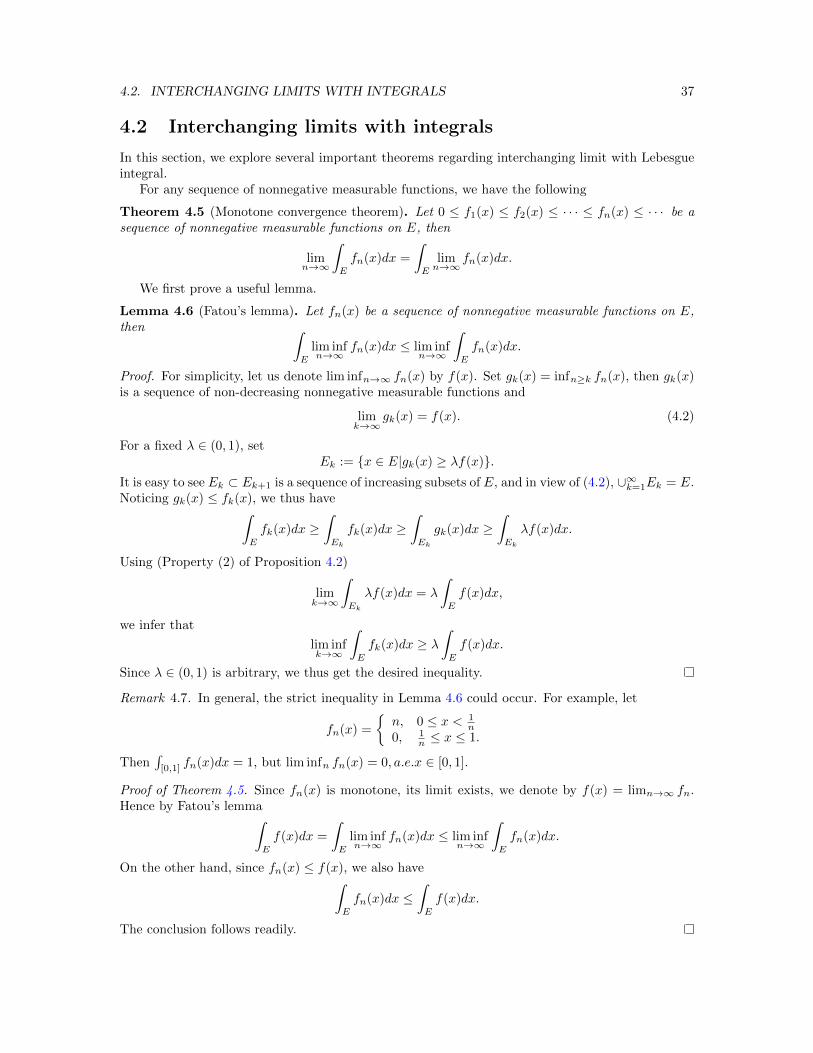
For any sequence of nonnegative measurable functions, we have the following
Theorem 4.5 (Monotone convergence theorem). Let 0 ≤ f1(x) ≤ f2(x) ≤ · · · ≤ fn(x) ≤ · · · be asequence of nonnegative measurable functions on E, then
limn→∞
∫E
fn(x)dx =
∫E
limn→∞
fn(x)dx.
We first prove a useful lemma.
Lemma 4.6 (Fatou’s lemma). Let fn(x) be a sequence of nonnegative measurable functions on E,then ∫
E
lim infn→∞
fn(x)dx ≤ lim infn→∞
∫E
fn(x)dx.
Proof. For simplicity, let us denote lim infn→∞ fn(x) by f(x). Set gk(x) = infn≥k fn(x), then gk(x)is a sequence of non-decreasing nonnegative measurable functions and
limk→∞
gk(x) = f(x). (4.2)
For a fixed λ ∈ (0, 1), setEk := x ∈ E|gk(x) ≥ λf(x).
It is easy to see Ek ⊂ Ek+1 is a sequence of increasing subsets of E, and in view of (4.2), ∪∞k=1Ek = E.Noticing gk(x) ≤ fk(x), we thus have∫
E
fk(x)dx ≥∫Ek
fk(x)dx ≥∫Ek
gk(x)dx ≥∫Ek
λf(x)dx.
Using (Property (2) of Proposition 4.2)
limk→∞
∫Ek
λf(x)dx = λ
∫E
f(x)dx,
we infer that
lim infk→∞
∫E
fk(x)dx ≥ λ∫E
f(x)dx.
Since λ ∈ (0, 1) is arbitrary, we thus get the desired inequality.
Remark 4.7. In general, the strict inequality in Lemma 4.6 could occur. For example, let
fn(x) =
n, 0 ≤ x < 1
n0, 1
n ≤ x ≤ 1.
Then∫
[0,1]fn(x)dx = 1, but lim infn fn(x) = 0, a.e.x ∈ [0, 1].
Proof of Theorem 4.5. Since fn(x) is monotone, its limit exists, we denote by f(x) = limn→∞ fn.Hence by Fatou’s lemma∫
E
f(x)dx =
∫E
lim infn→∞
fn(x)dx ≤ lim infn→∞
∫E
fn(x)dx.
On the other hand, since fn(x) ≤ f(x), we also have∫E
fn(x)dx ≤∫E
f(x)dx.
The conclusion follows readily.
38 CHAPTER 4. LEBESGUE’S INTEGRATION THEORY
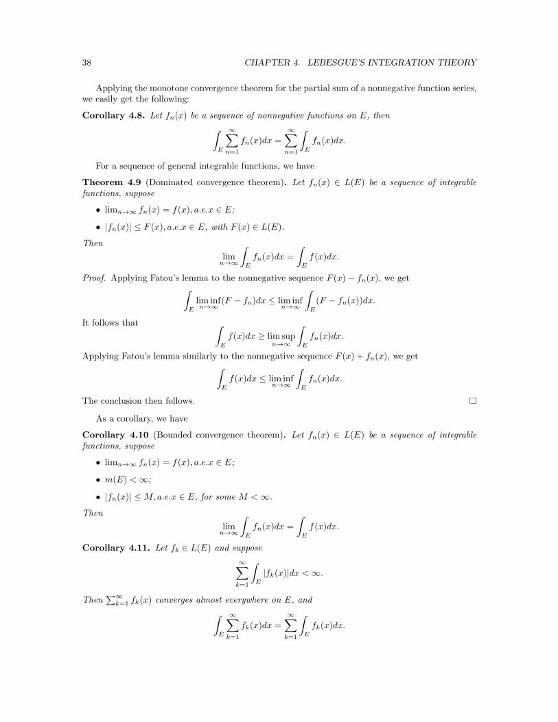
Applying the monotone convergence theorem for the partial sum of a nonnegative function series,we easily get the following:
Corollary 4.8. Let fn(x) be a sequence of nonnegative functions on E, then∫E
∞∑n=1
fn(x)dx =
∞∑n=1
∫E
fn(x)dx.
For a sequence of general integrable functions, we have
Theorem 4.9 (Dominated convergence theorem). Let fn(x) ∈ L(E) be a sequence of integrablefunctions, suppose
• limn→∞ fn(x) = f(x), a.e.x ∈ E;
• |fn(x)| ≤ F (x), a.e.x ∈ E, with F (x) ∈ L(E).
Then
limn→∞
∫E
fn(x)dx =
∫E
f(x)dx.
Proof. Applying Fatou’s lemma to the nonnegative sequence F (x)− fn(x), we get∫E
lim infn→∞
(F − fn)dx ≤ lim infn→∞
∫E
(F − fn(x))dx.
It follows that ∫E
f(x)dx ≥ lim supn→∞
∫E
fn(x)dx.
Applying Fatou’s lemma similarly to the nonnegative sequence F (x) + fn(x), we get∫E
f(x)dx ≤ lim infn→∞
∫E
fn(x)dx.
The conclusion then follows.
As a corollary, we have
Corollary 4.10 (Bounded convergence theorem). Let fn(x) ∈ L(E) be a sequence of integrablefunctions, suppose
• limn→∞ fn(x) = f(x), a.e.x ∈ E;
• m(E) <∞;
• |fn(x)| ≤M,a.e.x ∈ E, for some M <∞.
Then
limn→∞
∫E
fn(x)dx =
∫E
f(x)dx.
Corollary 4.11. Let fk ∈ L(E) and suppose
∞∑k=1
∫E
|fk(x)|dx <∞.
Then∑∞k=1 fk(x) converges almost everywhere on E, and∫
E
∞∑k=1
fk(x)dx =
∞∑k=1
∫E
fk(x)dx.
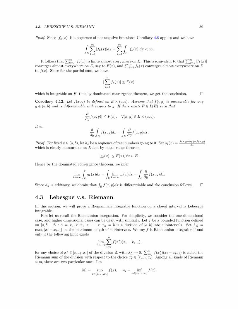
4.3. LEBESGUE V.S. RIEMANN 39
Proof. Since |fk(x)| is a sequence of nonnegative functions, Corollary 4.8 applies and we have∫E
∞∑k=1
|fk(x)|dx =
∞∑k=1
∫E
|fk(x)|dx <∞.
It follows that∑∞k=1 |fk(x)| is finite almost everywhere on E. This is equivalent to that
∑∞k=1 |fk(x)|
converges almost everywhere on E, say to F (x), and∑∞k=1 fk(x) converges almost everywhere on E
to f(x). Since for the partial sum, we have
|n∑k=1
fk(x)| ≤ F (x),
which is integrable on E, thus by dominated convergence theorem, we get the conclusion.
Corollary 4.12. Let f(x, y) be defined on E × (a, b). Assume that f(·, y) is measurable for anyy ∈ (a, b) and is differentiable with respect to y. If there exists F ∈ L(E) such that
| ∂∂yf(x, y)| ≤ F (x), ∀(x, y) ∈ E × (a, b),
thend
dy
∫E
f(x, y)dx =
∫E
∂
∂yf(x, y)dx.
Proof. For fixed y ∈ (a, b), let hk be a sequence of real numbers going to 0. Set gk(x) = f(x,y+hk)−f(x,y)hk
,which is clearly measurable on E and by mean value theorem
|gk(x)| ≤ F (x),∀x ∈ E.
Hence by the dominated convergence theorem, we infer
limk→∞
∫E
gk(x)dx =
∫E
limk→∞
gk(x)dx =
∫E
∂
∂yf(x, y)dx.
Since hk is arbitrary, we obtain that∫Ef(x, y)dx is differentiable and the conclusion follows.
4.3 Lebesgue v.s. Riemann
In this section, we will prove a Riemannian integrable function on a closed interval is Lebesgueintegrable.
Firs let us recall the Riemannian integration. For simplicity, we consider the one dimensionalcase, and higher dimensional cases can be dealt with similarly. Let f be a bounded function definedon [a, b]. ∆ : a = x0 < x1 < · · · < xn = b is a division of [a, b] into subintervals. Set λ∆ =maxi |xi − xi−1| be the maximum length of subintervals. We say f is Riemannian integrable if andonly if the following limit exists
limλ∆→0
n∑i=1
f(x∗i )(xi − xi−1),
for any choice of x∗i ∈ [xi−1, xi] of the division ∆ with λ∆ → 0.∑ni=1 f(x∗i )(xi − xi−1) is called the
Riemann sum of the division with respect to the choice x∗i ∈ [xi−1, xi]. Among all kinds of Riemannsum, there are two particular ones. Let
Mi = supx∈[xi−1,xi]
f(x), mi = infx∈[xi−1,xi]
f(x),
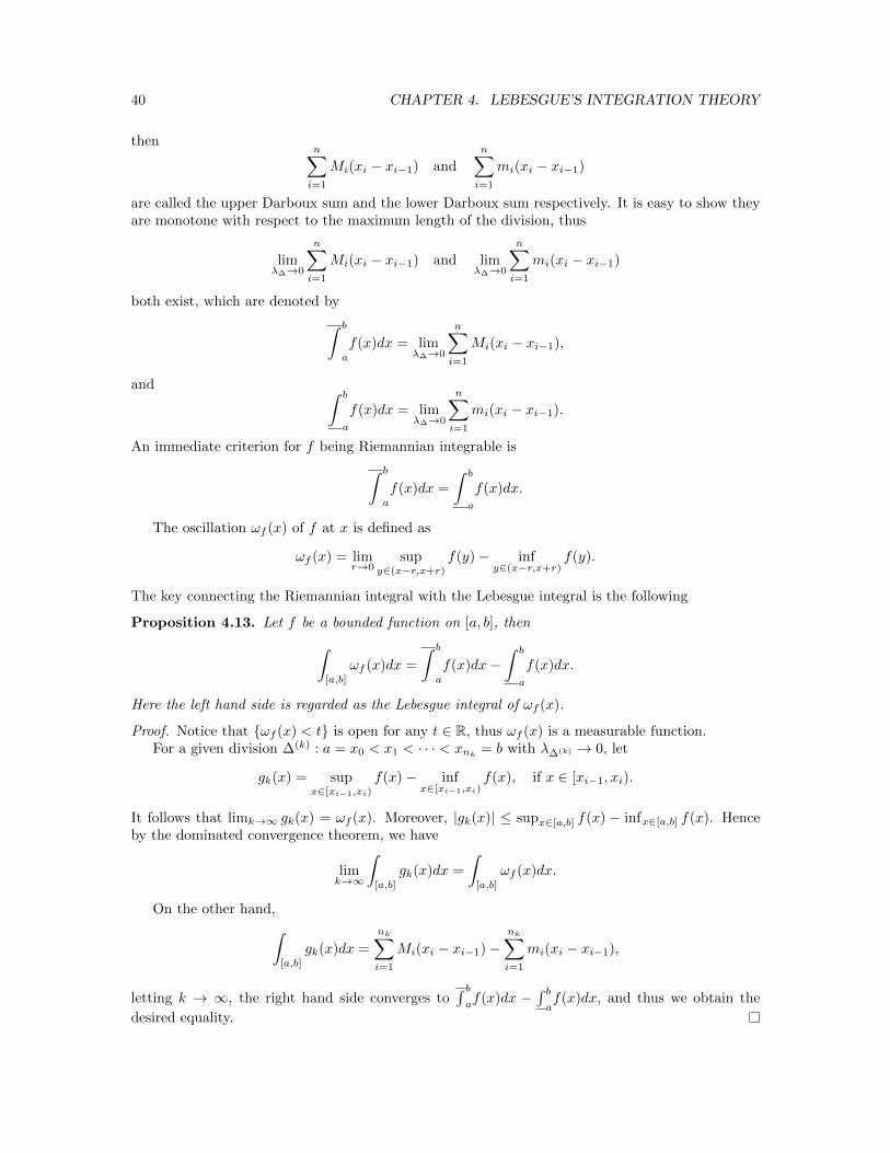
40 CHAPTER 4. LEBESGUE’S INTEGRATION THEORY
thenn∑i=1
Mi(xi − xi−1) and
n∑i=1
mi(xi − xi−1)
are called the upper Darboux sum and the lower Darboux sum respectively. It is easy to show theyare monotone with respect to the maximum length of the division, thus
limλ∆→0
n∑i=1
Mi(xi − xi−1) and limλ∆→0
n∑i=1
mi(xi − xi−1)
both exist, which are denoted by∫ b
a
f(x)dx = limλ∆→0
n∑i=1
Mi(xi − xi−1),
and ∫ b
a
f(x)dx = limλ∆→0
n∑i=1
mi(xi − xi−1).
An immediate criterion for f being Riemannian integrable is∫ b
a
f(x)dx =
∫ b
a
f(x)dx.
The oscillation ωf (x) of f at x is defined as
ωf (x) = limr→0
supy∈(x−r,x+r)
f(y)− infy∈(x−r,x+r)
f(y).
The key connecting the Riemannian integral with the Lebesgue integral is the following
Proposition 4.13. Let f be a bounded function on [a, b], then∫[a,b]
ωf (x)dx =
∫ b
a
f(x)dx−∫ b
a
f(x)dx.
Here the left hand side is regarded as the Lebesgue integral of ωf (x).
Proof. Notice that ωf (x) < t is open for any t ∈ R, thus ωf (x) is a measurable function.For a given division ∆(k) : a = x0 < x1 < · · · < xnk = b with λ∆(k) → 0, let
gk(x) = supx∈[xi−1,xi)
f(x)− infx∈[xi−1,xi)
f(x), if x ∈ [xi−1, xi).
It follows that limk→∞ gk(x) = ωf (x). Moreover, |gk(x)| ≤ supx∈[a,b] f(x) − infx∈[a,b] f(x). Henceby the dominated convergence theorem, we have
limk→∞
∫[a,b]
gk(x)dx =
∫[a,b]
ωf (x)dx.
On the other hand,∫[a,b]
gk(x)dx =
nk∑i=1
Mi(xi − xi−1)−nk∑i=1
mi(xi − xi−1),
letting k → ∞, the right hand side converges to∫ baf(x)dx −
∫ baf(x)dx, and thus we obtain the
desired equality.
4.4. FUBINI’S THEOREM 41
Corollary 4.14. Let f be a bounded function on [a, b], f is Riemannian integrable if and only ifthe set of points of discontinuity has measure zero.
Proof. By Proposition 4.13, f is Riemannian integrable if and only if∫[a,b]
ωf (x)dx = 0.
However, ωf (x) ≥ 0 by definition. Hence ωf (x) = 0, a.e.x ∈ [a, b]. The conclusion follows since f iscontinuous at x if and only if ωf (x) = 0.
Finally, we prove the main theorem of this section.
Theorem 4.15. Let f be a Riemannian integrable function on [a, b], then f is Lebesgue integrable,and ∫ b
a
f(x)dx =
∫[a,b]
f(x)dx.
Proof. Since f is Riemannian integrable, it is continuous almost everywhere, thus f is a measurablefunction. By definition it is bounded, therefore it is Lebesgue integrable. Take any division ∆ of[a, b], say ∆ : a = x0 < x1 < · · · < xn = b, we have
n∑i=1
mi(xi − xi−1) ≤n∑i=1
∫[xi−1,xi]
f(x)dx =
∫[a,b]
f(x)dx ≤n∑i=1
Mi(xi − xi−1).
Letting λ∆ → 0, we get the desired conclusion.
Remark 4.16. Riemannian improper integral does not have direction relation with Lebesgue integral.For example, f(x) = sin x
x is integrable on (0,∞) as Riemannian improper integral, however, it isnot Lebesgue integrable on (0,∞).
4.4 Fubini’s Theorem
In this section, we prove the Fubini’s theorem. This is a very useful theorem which turns a Lebesgueintegration of f(x, y) defined on Rm = Rp × Rq 3 (x, y) into iterated integrals
∫Rp dx
∫Rq fx(y)dy.
For a fixed x or y, we define the slice of f as
fx(y) : Rq → R,
andfy(x) : Rp → R.
The question in mind is whether∫Rm
f(x, y)dxdy =
∫Rpdx
∫Rqfx(y)dy =
∫Rqdy
∫Rpfy(x)dx? (4.3)
The starting point is that f(x, y) is a measurable function on Rm. To make sense of (5.5),one needs to verify first that slices fx(y) and fy(x) are measurable and integrable, and then theirintegrals
∫Rp fy(x)dx,
∫Rq fx(y)dy are also measurable and integrable. Fubini’s theorem asserts once
f is Lebesgue integrable on Rm, the dubious issues settle automatically.
Theorem 4.17 (Fubini). Let f ∈ L(Rm), then
1. fx(y) is integrable a.e.x ∈ Rp;

42 CHAPTER 4. LEBESGUE’S INTEGRATION THEORY
2.∫Rp fx(y)dy is integrable;
3.∫Rm f(x, y)dxdy =
∫Rp dx
∫Rq fx(y)dy.
Since x, y are symmetric, interchanging x and y, we also get∫Rm f(x, y)dxdy =
∫Rq dy
∫Rp fy(x)dx
provided f ∈ L(Rm).
Proof. Denote the set of integrable functions on Rm which satisfy 1-3 by F , we shall show allintegrable functions belong to F . This goal is achieved, as a usual scheme in this note, by firstshowing our building blocks (characteristic functions) belong to F and then proving operations suchas linear combination and limits are closed in F . We also note 1-2 are necessary conditions for 3to hold. Indeed, if f ∈ L(Rm) and 3 holds, then
∫Rq fx(y)dy is integrable on Rp, and thus is finite
almost everywhere, which implies fx(y) is integrable a.e.x ∈ Rp. So the most important property tocheck is 3.
Step 1 Linear combinations of functions in F is in F . Since we are mainly concerned withproperty 3, this follows directly from the linear property of Lebesgue integration.
Step 2 Let 0 ≤ f1 ≤ f2 ≤ · · · fn · · · be an increasing sequence of nonnegative functions in F .Suppose limn→∞ fn = f and f is integrable, then f ∈ F .
By assumption, for each i, there exists Ai ⊂ Rp of measure zero, such that fi,x(y) is integrablefor x /∈ Ai. Let A = ∪iAi, then m(A) = 0 and fi,x(y) is integrable for x /∈ A for every i. Bymonotone convergence theorem, for each fixed x /∈ A, we have
limi→∞
∫Rqfi,x(y)dy =
∫Rqfx(y)dy.
Appealing to the monotone convergence theorem again, we have
limi→∞
∫Rp
∫Rqfi,x(y)dydx =
∫Rp
∫Rqfx(y)dydx.
By assumption, the term on the left hand side is∫Rn fi(x, y)dxdy, and monotone convergence theorem
once again tells
limi→∞
∫Rm
fi(x, y)dxdy =
∫Rm
f(x, y)dxdy.
Thus ∫Rm
f(x, y)dxdy =
∫Rp
∫Rqfx(y)dydx.
Since f is integrable, it follows ∫Rqfx(y)dy <∞, a.e.x ∈ Rp.
Above two formula justify 1-3, and thus f ∈ F .
Step 3 χE ∈ F , where E is a Gδ set of finite measure. We break into several steps.
step 3.1 χE ∈ F provide E is a cube. (open, closed, half-open half closed)
step 3.2 χE ∈ F if E is an open set. Since any open set can be written as disjoint union of half-openhalf-closed cubes. Appealing to the step 2 on the monotone limits, we get desired conclusion.
step 3.3 If E is a Gδ set of finite measure, we may assume that E = ∩nGn, where each Gn is anopen set of finite measure. Then use monotone decreasing limit of step 2.
4.4. FUBINI’S THEOREM 43
Step 4 χE ∈ F , where E is a set of measure zero. There exists a Gδ set, say G ⊃ E, andm(G) = 0. By Step 3, we have
0 = m(G) =
∫Rm
χGdxdy =
∫Rpdx
∫RqχG,x(y)dy.
Since χG is nonnegative, it follows∫RqχG,x(y)dy = 0, a.e.x ∈ Rp.
Since 0 ≤ χE ≤ χG, we have ∫RqχE,x(y)dy = 0, a.e.x ∈ Rp.
Thus∫Rq χE,x(y)dy in integrable a.e.x ∈ Rp and∫
Rp
∫RqχE,x(y)dy = 0 =
∫Rm
χE(x, y)dxdy = m(E) = 0.
Step 5 χE ∈ F , where E is a measurable set of finite measure. Since any measurable set differsfrom a Gδ set by a set of measure zero. This step is achieved by Step 4 and Step 5.
Step 6 Any integrable functions are in F . Let f be an integrable function, then f+ and f− areboth integrable. There exist two increasing sequences of simple functions ϕn f+ and ψ f−.Each simple function belongs to F by Step 5, Step 1. Hence f± ∈ F by Step 2. Finally f ∈ F byStep 1.
An implicit fact of this theorem is that if f(x, y) is Lebesgue measurable, then fx(y) is measurablea.e.x ∈ Rp and
∫Rq fx(y)dy is measurable as a function of x ∈ Rp. When restricting to nonnegative
measurable functions, we have
Theorem 4.18 (Tonelli). Let f(x, y) be a nonnegative measurable function, then
1. fx(y) is nonnegative measurable a.e.x ∈ Rp;
2.∫Rp fx(y)dy is nonnegative measurable;
3.∫Rm f(x, y)dxdy =
∫Rp dx
∫Rq fx(y)dy.
Proof. We consider a truncation of f as follows:
fk(x, y) :=
f(x, y), if f(x, y) < k and x2 + y2 < k2
0, else.
Clearlyfk(x, y) f(x, y), fk,x(y) fx(y),
and fk(x, y) is integrable. A repetition of Step 2 in the proof of Fubini theorem shows that∫Rp
∫Rqfx(y)dydx =
∫Rm
f(x, y)dxdy.
fk,x(y) is measurable for x ∈ Eck with m(Ek) = 0. Let E = ∪∞k=1Ek, then m(E) = 0 andfx(y) = limk→∞ fk,x(y) as a limit of measurable functions for x /∈ E, thus is measurable.
Similarly, by the monotone convergence theorem,
limk→∞
∫Rqfk,x(y)dy =
∫Rqfx(y)dy.
Since∫Rq fk,x(y)dy is integrable, thus measurable.
∫Rq fx(y)dy as a limit of sequence of measurable
functions is also measurable.

44 CHAPTER 4. LEBESGUE’S INTEGRATION THEORY
The Tonelli theorem, in practice, is usually combined with the Fubini theorem. For example, inorder to show a particular function f is integrable on Rm and compute its integral, one can firstlook at |f |, using Tonelli theorem to turn the integral of |f | on Rm into an iterated integral, whichhopefully can be evaluated explicitly. Given that integral is finite, it implies f is integrable. Thusthe condition of Fubini theorem is satisfied, and another round the iterated integral for f is now inposition.
Finally, we use the Fubini theorem to point out a useful formula which indicates the geometricmeaning of Lebesgue integrals.
Let f be a nonnegative measurable function defined on E ⊂ Rn. Then its graph is defined asthe set
Gf := (x, y) ∈ Rn+1|x ∈ E, y = f(x).
The region below the graph is thus
G := (x, y) ∈ Rn+1|x ∈ E, 0 ≤ y ≤ f(x).
Proposition 4.19. Let m denote the Lebesgue measure of Rn+1, suppose f is integrable on E, then∫E
f(x)dx = m(G).
Proof. Approximating f by simple functions imply that G is a measurable set in Rn+1, thus χG(x, y)is a nonnegative measurable function. Apply Tonelli’s theorem, we get
m(G) =
∫Rn+1
χG(x, y)dxdy =
∫E
dx
∫ f(x)
0
1dy =
∫E
f(x)dx.
We can also consider the other order of the iterated integration:∫Rn+1
χG(x, y)dxdy =
∫Rdy
∫RnχG(x, y)dx =
∫ ∞0
m(x ∈ E|f(x) ≥ y)dy.
This yields
Proposition 4.20. Let f(x) ∈ L(E), then∫E
f(x)dx =
∫ ∞0
m(x ∈ E|f(x) ≥ y)dy.
The right hand side can be viewed as evaluating the volume under the graph horizontally.
Chapter 5
Differentiation
9)Q§ûÝ\8j"¬'ýº§A¯ì"
))Ú75"6
The goal of this chapter to explore the fundamental theorem of Calculus in Lebesgue integrationtheory. The fundamental theorem of Calculus has two-fold conclusions:
• suppose f(x) is Riemannian integrable on [a, b]. Let F (x) =∫ xaf(t)dt, then F is differentiable
at x if f is continuous at x and F ′(x) = f(x).
• If F ′(x) is Riemannian integrable on [a, b], then
F (x)− F (a) =
∫ x
a
F ′(t)dt.
We are concerned with above two statements when Riemannian integrable is replaced by Lebesgueintegrable. We shall answer the following two questions in this chapter.
• given f ∈ L([a, b]), let F (x) =∫
[a,x]f(t)dt, whether F (x) is differentiable (continuous), and if
it is, does F ′(x) = f(x)?
• suppose F ′(x) is Lebesgue integrable, does F (x)− F (a) =∫ xaF ′(t)dt hold?
5.1 Monotone functions
This section is devoted to the proof of the following famous theorem of Lebesgue.
Theorem 5.1 (Lebesgue). Suppose f is a monotone function defined on an open interval (a, b),then f is differentiable almost everywhere.
This is a striking and deep theorem. A basic fact about monotone function is that it has atmost countable many discontinuous points. While the differentiability property seems to come fromnowhere. The idea is to quantify the set of non-differentiable points, and use a set theoretic coveringlemma due to Vitali.
45
46 CHAPTER 5. DIFFERENTIATION
We recall first the upper derivative and the lower derivative of f at x:
Df(x) = limh→0
[sup
0<|t|≤h
f(x+ t)− f(x)
t
];
Df(x) = limh→0
[inf
0<|t|≤h
f(x+ t)− f(x)
t
].
Clearly, both Df(x) and Df(x) exit and Df(x) ≥ Df(x). It is readily seen that f is differentiableat x if and only if Df(x) = Df(x).
Thus the set of non-differentiable points of f is
E := x ∈ (a, b)|Df(x) > Df(x).
A quantified version of E is that
E = ∪α>β,α,β∈QEα,β ,
where Eα,β := x ∈ E|Df(x) > α > β > Df(x). In order to show f is differentiable almosteverywhere, it suffices to prove that m∗(Eα,β) = 0, for any pair of rational numbers α > β.
Now we state the Vitali covering lemma, which is of great usage.
Definition 5.2. A collection of closed intervals F is called a Vitali covering of E, if ∀ε > 0 andx ∈ E, there exists a closed interval in F of length less ε containing x.
Lemma 5.3 (Vitali covering lemma). Suppose E ⊂ R is of finite outer measure, and F is a Vitalicovering of E, then for any ε > 0, there exist finite many disjoint Ik ∈ F , k = 1, · · · , N , such that
m∗(E \ (∪Nk=1Ik)) < ε and m∗((∪Nk=1Ik) \ E) < ε.
Proof. Since m∗(E) <∞, there exists an open set G ⊃ E with m(G) <∞ and m∗(G \ E) < ε. Wemay assume all intervals in F are contained in G. Hence δ1 := supI∈F |I| <∞.
We shall choose successively disjoint intervals from F , the first one we choose satisfies |I1| > δ12 .
Setδn = sup|I||I ∈ F ,which is disjoint from I1, · · · In−1,
and we choose In+1 disjoint from I1, · · · , In−1, with |In| > δn2 .
This process either stops after finite many steps (which furnishes the proof already), or continuesto yield a countable disjoint intervals In, with
|In| >δn2, ∪∞n=1In ⊂ E ⊂ G.
Therefore∞∑n=1
|In| < m∗(E) <∞,
which implies that limn→∞ δn = 0. It follows for any ε > 0, there exists N such that
∞∑n=N+1
|In| <ε
5.
Let 5I denote the dilation of I by 5 times, we claim
E \ ∪Nn=1In ⊂ ∪∞n=N+15In.
5.1. MONOTONE FUNCTIONS 47
Take any x ∈ E \ (∪Nn=1In), since F is a Vitali covering of E, there exists a closed interval Ixdisjoint from I1, · · · , IN containing x. In view of limn→∞ δn = 0, Ix must intersect with Ik for somek > N . (otherwise δn ≥ |Ix|, ∀n) Let k be the smallest number such that Ix ∩ Ik 6= ∅, then we have
|Ix| ≤ δk, |Ik| >δk2.
A simple geometry shows that Ix ⊂ 5Ik−1. The desired claim follows.Finally,
m∗(E \ (∪Nn=1In)) ≤∞∑
n=N+1
5|In| < ε.
The second conclusion is by virtue of
m∗((∪nk=1Ik) \ E) < m∗(G \ E) < ε.
Now we present the proof of the Lebesgue theorem.
Proof. Without loss of generality, we may assume f is monotone increasing. As elucidate above, ourgoal is to show that m∗(Eα,β) = 0. By definition of Eα,β , we see
F(β) := [a, b]|f(b)− f(a)
b− a< β,
and
F(α) := [c, d]|f(d)− f(c)
d− c> α,
are both Vitali coverings of Eα,β . Indeed, for x ∈ F(α) and ε > 0, by definition there exists a closed
interval of the form [x− h, x] or [x, x+ h] with h < ε such that f(x+h)−f(x)h > α, or f(x)−f(x−h)
h > α.Similarly one can check it for F(β).
Since Eα,β ⊂ (a, b) is of finite outer measure, by Vitali covering lemma, ∀ε > 0, there exist finitedisjoint intervals [ai, bi] ∈ F(β), i = 1, · · · , n, such that
m∗(Eα,β \ (∪ni=1[ai, bi])) < ε and m∗((∪ni=1[ai, bi]) \ Eα,β) < ε. (5.1)
Set Ei = Eα,β ∩ (ai, bi) and apply the Vitali covering lemma to the family F(α), we get for each
i, finite many intervals [c(i)j , d
(i)j ] ∈ F(α), j = 1, · · · , ik satisfying
m∗(Ei \ (∪ikj=1[c(i)j , d
(i)j ])) < ε. (5.2)
Thus
α(d(i)j − c
(i)j ) < f(d
(i)j )− f(c
(i)j ),
and adding from j = 1 to ik, we get
α
ik∑j=1
(d(i)j − c
(i)j ) <
ik∑j=1
(f(d(i)j )− f(c
(i)j )) ≤ f(bi)− f(ai), (5.3)
where the last inequality is due to the fact that f is monotone increasing and [cj , dj ] are disjointfrom each other.
48 CHAPTER 5. DIFFERENTIATION
By (5.2), we haveik∑j=1
(d(i)j − c
(i)j ) > m∗(Ei)− ε.
Since [ai, bi] ∈ F(β), we proceed (5.3) as follows
α(m∗(Ei)− ε) < f(bi)− f(ai) < β(bi − ai).
Adding from i = 1 to n, we obtain
α(m∗ (Eα,β ∩ (∪ni=1[ai, bi]))− nε) < β
n∑i=1
(bi − ai). (5.4)
By (5.1), we havem∗(Eα,β ∩ (∪ni=1[ai, bi])) > m∗(Eα,β)− ε,
andn∑i=1
(bi − ai) ≤ (m∗(Eα,β) + ε).
Plugging these back to (5.4), we deduce that
(α− β)m∗(Eα,β) < (α(n+ 1) + β)ε.
Since ε is arbitrary, we infer m∗(Eα,β) = 0, and the proof is completed.
Corollary 5.4. Suppose f is a monotone increasing function on [a, b], then f ′ is integrable and∫[a,b]
f ′(x)dx ≤ f(b)− f(a). (5.5)
Proof. Extend f to take value f(b) on (b, b+ 1]. We let
fn = n(f(x+1
n)− f(x)), x ∈ [a, b].
It is easy to see that fn(x) is measurable. Then by Lebesgue’s theorem on the almost everywheredifferentiability of f , we have
limn→∞
fn(x) = f ′(x), a.e., x ∈ [a, b].
Thus f ′(x) is also measurable. By Fatou’s lemma, we get∫[a,b]
f ′(x)dx ≤ lim infn→∞
∫[a,b]
fn(x)dx.
Noticing ∫[a,b]
fn(x)dx = n
∫[b,b+ 1
n ]
f(x)dx− n∫
[a,a+ 1n ]
f(x)dx ≤ f(b)− f(a),
thus we get the desired inequality.
Remark 5.5. Let f be a continuous function on [a, b], which is differentiable on (a, b), one cann’tgenerally infer that f ′(x) is integrable without the assumption of monotonicity. Here is an example
f(x) =
x2 sin( 1
x2 ), x ∈ (0, 1]0, x = 0.
. (5.6)
5.2. FUNDAMENTAL THEOREM OF CALCULUS I 49
Remark 5.6. The strict inequality can occur in (5.5). For example, we simply take a step function,i.e.,
f(x) =
0, 0 ≤ x ≤ 1
21, 1
2 < x ≤ 1
A more interesting example is the Cantor function.Recall that Cantor set is resulted from [0, 1] by removing ’the middle third’ intervals consecutively.
Thus ∀x ∈ C, it has a decimal representation of base 3
x = 2
∞∑i=1
ai3i, ai ∈ 0, 1.
For each such x, define
ϕ(x) =
∞∑i=1
ai2i.
If follows that ϕ maps C onto [0, 1]. The Cantor function is define as follows
Ψ(x) = supϕ(y)|y ≤ x, y ∈ C, x ∈ [0, 1].
A moment of thought reveals that Ψ(x) satisfies
• Ψ(0) = 0 and Ψ(1) = 1;
• Ψ(x) is monotone increasing;
• Ψ(x) is continuous;
• Ψ′(x) = 0 almost everywhere, since it is constant on those ’middle third’ intervals.
5.2 Fundamental theorem of Calculus I
In this section, we answer the first question of the fundamental theorem of integral Calculus: givenf ∈ L([a, b]), let F (x) =
∫[a,x]
f(t)dt, whether F ′(x) = f(x)? Since modifying the value of the
integrand on a set of measure zero does not affect the value of F (x), we can only expect F ′(x) = f(x)holds almost everywhere.
Theorem 5.7. Let f ∈ L([a, b]) and F (x) =∫
[a,x]f(t)dt, then
F ′(x) = f(x), a.e., x ∈ [a, b].
Proof. We first claim that F (x) is differentiable almost everywhere. Indeed,
F (x) =
∫[a,x]
f(t)dt =
∫[a,x]
f+(t)dt−∫
[a,x]
f−(t)dt.
It is easy to see both∫
[a,x]f+(t)dt and
∫[a,x]
f−(t)dt are monotone functions. Thus by Lebesgue’s
theorem, F is differentiable almost everywhere.We extend f by 0 for x /∈ [a, b]. Let Fh(x) = 1
h
∫[x,x+h]
f(t)dt, thus
limh→0
Fh(x) = F ′(x), a.e., x ∈ [a, b].
We next claim that
limh→0
∫[a,b]
|Fh(x)− f(x)|dx = 0. (5.7)

50 CHAPTER 5. DIFFERENTIATION
To see this, we have∫[a,b]
|Fh(x)− f(x)|dx ≤∫
(−∞,+∞)
|Fh(x)− f(x)|dx
=
∫(−∞,+∞)
| 1h
∫[x,x+h]
f(t)− f(x)dt|dx
≤∫
(−∞,+∞)
1
h
∫[x,x+h]
|f(t)− f(x)|dtdx
≤∫
(−∞,+∞)
1
h
∫[0,h]
|f(x+ t)− f(x)|dtdx
≤∫
[0,h]
1
h
∫(−∞,+∞)
|f(x+ t)− f(x)|dxdt. (5.8)
By Theorem 4.4,
limt→0
∫(−∞,+∞)
|f(x+ t)− f(x)|dx = 0.
Thus, for ε > 0, there exists δ > 0, such that∫(−∞,+∞)
|f(x+ t)− f(x)|dx < ε, ∀|t| < δ.
Therefore, for |h| < δ, we proceed (5.8) as∫[a,b]
|Fh(x)− f(x)|dx ≤∫
[0,h]
1
hεdt = ε.
The claim then follows.Finally, by Fatou’s lemma, we have∫
[a,b]
lim inf |Fh(x)− f(x)|dx ≤ lim inf
∫[a,b]
|Fh(x)− f(x)|dx = 0.
Thus ∫[a,b]
|F ′(x)− f(x)|dx = 0,
which implies F ′(x) = f(x) almost everywhere.
5.2.1 A detour: Bounded variation functions
As alluded to in the above proof, we express F (x) as the difference of two monotone functions. Inthis subsection, we take a detour to prove Jordan’s theorem which characterizes functions that aredifference of monotone functions, the functions of bounded variation.
Let f be a real-valued function defined on [a, b], let P : a = x0 < x1 < · · ·xn = b be a partition,then the variation of f with respect to P is defined as
V (f, P ) =
n∑i=1
|f(xi)− f(xi−1)|.
The total variation of f on [a, b] is defined as
TV (f) := supV (f, P )|P is a partition of [a, b].

5.2. FUNDAMENTAL THEOREM OF CALCULUS I 51
Definition 5.8. A real-valued function f defined on [a, b] is said to be bounded variation if
TV (f) <∞.
It is denoted by f ∈ BV([a, b]).
Example 12. Let f be an increasing function on [a, b], then
TV (f) = f(b)− f(a).
Example 13. Let f be a Lipschitz continuous function on [a, b], i.e., |f(x) − f(y)| ≤ L|x − y|,∀x, y ∈ [a, b]. Then f ∈ BV([a, b]).
Proof. For any partition P : a = x0 < x1 < · · ·xn = b,
V (f, P ) =
n∑i=1
|f(xi)− f(xi−1)| ≤ Ln∑i=1
|xi − xi−1| = L(b− a).
Similarly, if f is a function on [a, b] such that |f ′(x)| ≤M , then f ∈ BV([a, b]).Now we state our main theorem of this section.
Theorem 5.9 (Jordan). Let f ∈ BV([a, b]) if and only if f is the difference of two monotonefunctions.
For the proof, we need
Lemma 5.10. Let f ∈ BV([a, b]), and c ∈ (a, b), then
b∨a
(f) =
c∨a
(f) +
b∨c
(f).
Here
b∨a
(f) refers to the total variation of f on [a, b].
Proof. First, take a partition P of [a, b], say P : a = x0 < x1 < · · · < xn = b. Insert c into thispartition. More precisely, there exists i such that xi−1 ≤ c ≤ xi, and we consider Pcl : a = x0 <· · · < xi−1 ≤ c and Pcr : c ≤ xi · · · < xn = b, which form partitions of [a, c] and [c, b] respectively.Clearly
V (f, P ) ≤ V (f, Pcl) + V (f, Pcr),
by triangle inequality. Thus
V (f, P ) ≤c∨a
(f) +b∨c
(f), ∀P.
It follows that∨ba(f) ≤
∨ca(f) +
∨bc(f).
For the reversed direction, ∀ε > 0 there exists two partitions P1 and P2 of [a, c] and [c, b]respectively, such that
c∨a
(f)− ε
2≤ V (f, P1),
b∨c
(f)− ε
2≤ V (f, P2).
Let P be the partition joined by P1 and P2, thus
b∨a
(f) ≥ V (f, P ) = V (f, P1) + V (f, P2) ≥c∨a
(f) +
b∨c
(f)− ε.
Since ε is arbitrary, we get∨ba(f) ≥
∨ca(f) +
∨bc(f). This completes the proof.
52 CHAPTER 5. DIFFERENTIATION
Proof of Theorem 5.9.
• ⇒We show if f ∈ BV([a, b]), then it can be written as the difference of two monotone functions.Let
g(x) =1
2(
x∨a
(f) + (f)), h(x) =1
2(
x∨a
(f)− f(x)).
It follows that f(x) = g(x)− h(x). Now we show g(x), h(x) are monotone. Indeed, for x ≤ y,
g(y)− g(x) =1
2(
y∨a
(f)−x∨a
(f) + f(y)− f(x))
=1
2(
y∨x
(f) + f(y)− f(x)) ≥ 0.
Here we have used Lemma 5.10.
The monotonicity of h is similar.
• ⇐ Suppose f(x) = g(x)− h(x), where g(x), h(x) are two monotone functions. It is routine tocheck that BV([a, b]) is indeed a linear vector space, thus f ∈ BV([a, b]) as both g and h arebounded variation in [a, b].
5.3 Fundamental theorem of Calculus II
In this section we answer the second question of the fundamental theorem of integral calculus: when
f(b)− f(a) =
∫[a,b]
f ′(t)dt
holds provided that f ′(x) ∈ L([a, b])?Let g(x) =
∫[a,x]
f ′(t)dt, by definition
g(b)− g(a) =
∫[a,b]
f ′(t)dt.
By Theorem 5.7, we also know g′(x) = f ′(x), a.e., x ∈ [a, b].Thus the question reduces to show that g − f = constant, provided (g − f)′ = 0, a.e, x ∈ [a, b].
This is not always true. For example, the Cantor function is a nonconstant function whose derivativeis zero almost everywhere. How to exclude such examples? We introduce the concept of absolutelycontinuity. In the following lemma, we shall see this concept exactly prevents wired behavior likeCantor function to occur.
Definition 5.11. A real valued function f on [a, b] is called absolutely continuous, if ∀ε > 0,
there exists δ > 0, such that for any finite many disjoint intervals (xi, yi)ni=1 with
n∑i=1
(yi−xi) < δ,
there holdsn∑i=1
|f(xi)− f(yi)| < ε.
The collection of absolutely continuous functions on [a, b] is denoted by AC([a, b]).

5.3. FUNDAMENTAL THEOREM OF CALCULUS II 53
Lemma 5.12. Suppose f ′(x) = 0, a.e., x ∈ [a, b] and f is not a constant, then ∃ε > 0, such that
∀δ > 0, there exists finite many disjoint intervals (xi, yi) with
n∑i=1
(yi − xi) < δ, such that
n∑i=1
|f(xi)− f(yi)| > ε.
Proof. Without loss of generality, we may assume f(a) 6= f(b). Let A be the set where f ′(x) = 0.Thus m(A) = b − a. For a fixed λ which to be determined momentarily, we consider the family ofclosed intervals:
F := [c, d]| |f(c)− f(d)|d− c
< λ.
It is easy to see F forms a Vitali covering of A. Therefore, ∀δ > 0, there exists a finite many disjointintervals [ci, di] ∈ F , i = 1, · · · , n, such that
m(A \ (∪ni=1[ci, di])) < δ.
The complement of (∪ni=1[ci, di]) in (a, b) is finite many disjoint intervals, (xj , yj), j = 1, · · · , k. Wehave
|f(b)− f(a)| ≤k∑j=1
|f(xj)− f(yj)|+n∑i=1
|f(ci)− f(di)|
≤k∑j=1
|f(xj)− f(yj)|+ λ
n∑i=1
|ci − di| <k∑j=1
|f(xj)− f(yj)|+ λ(b− a).
If we choose λ = |f(a)−f(b)|2(b−a) , it follows
k∑j=1
|f(xj)− f(yj)| >|f(a)− f(b)|
2:= ε,
with∑kj=1 |xj − yj | = m(A \ (∪ni=1[ci, di])) < δ.
It immediately follows
Theorem 5.13. If f is absolutely continuous on [a, b] and f ′(x) = 0, a.e., x ∈ [a, b], then f =constant.
Theorem 5.14. If f ∈ AC([a, b]) then f ∈ BV([a, b]).
Proof. Since f is absolutely continuous, for ε = 1, there exists δ > 0, such that for any finite many
disjoint intervals (xi, yi)ni=1 with
n∑i=1
(yi − xi) < δ, we have
n∑i=1
|f(xi)− f(yi)| < 1. (5.9)
We take a partition of P : a = z0 < z1 < · · · < zn = b, such that the length of each subinterval isless than δ. It follows from (5.9) that
zi∨zi−1
(f) < 1, i = 1, · · · , n.
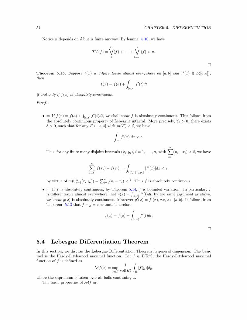
54 CHAPTER 5. DIFFERENTIATION
Notice n depends on δ but is finite anyway. By lemma 5.10, we have
TV (f) =
z1∨a
(f) + · · ·+b∨
zn−1
(f) < n.
Theorem 5.15. Suppose f(x) is differentiable almost everywhere on [a, b] and f ′(x) ∈ L([a, b]),then
f(x) = f(a) +
∫[a,x]
f ′(t)dt
if and only if f(x) is absolutely continuous.
Proof.
• ⇒ If f(x) = f(a) +∫
[a,x]f ′(t)dt, we shall show f is absolutely continuous. This follows from
the absolutely continuous property of Lebesgue integral. More precisely, ∀ε > 0, there existsδ > 0, such that for any F ⊂ [a, b] with m(F ) < δ, we have∫
F
|f ′(x)|dx < ε.
Thus for any finite many disjoint intervals (xi, yi), i = 1, · · · , n, with
n∑i=1
(yi−xi) < δ, we have
n∑i=1
|f(xi)− f(yi)| =∫∪ni=1[xi,yi]
|f ′(x)|dx < ε,
by virtue of m(∪ni=1[xi, yi]) =∑ni=1(yi − xi) < δ. Thus f is absolutely continuous.
• ⇐ If f is absolutely continuous, by Theorem 5.14, f is bounded variation. In particular, fis differentiable almost everywhere. Let g(x) =
∫[a,x]
f ′(t)dt, by the same argument as above,
we know g(x) is absolutely continuous. Moreover g′(x) = f ′(x), a.e, x ∈ [a, b]. It follows fromTheorem 5.13 that f − g = constant. Therefore
f(x) = f(a) +
∫[a,x]
f ′(t)dt.
5.4 Lebesgue Differentiation Theorem
In this section, we discuss the Lebesgue Differentiation Theorem in general dimension. The basictool is the Hardy-Littlewood maximal function. Let f ∈ L(Rn), the Hardy-Littlewood maximalfunction of f is defined as
Mf(x) = supx∈B
1
vol(B)
∫B
|f(y)|dy,
where the supremum is taken over all balls containing x.The basic properties of Mf are
5.4. LEBESGUE DIFFERENTIATION THEOREM 55
Proposition 5.16. Let f ∈ L(Rn), then
• M(f) is measurable;
• M(f)(x) <∞, a.e.x;
• Weak L1 inequality:
m(x ∈ Rn|M(f)(x) > α) ≤ 3n
α
∫Rn|f(x)|dx, ∀α > 0.
The technical part is the weak L1 inequality. We need the following covering lemma.
Lemma 5.17. Let Bri(xi)i∈I be a collection of finite many balls. Then there exists a disjointsub-collection J ⊂ I, Brj (xj)j∈J such that
∪j∈JB3rj (xj) ⊃ ∪i∈IBri(xi).
Proof. This is also a version of Vitali covering lemma and the proof is similar. First choose a ball oflargest radius, say Br1(x1). We then throw away all balls that intersect with Br1(x1). Pick a ballof largest radius among the remaining balls, say Br2(x2). Throw away all balls that intersect withBr2(x2). Iterate this process until there is no ball left. What we picked out is the desired collection,as enlarging each’s radius by 3 times would contain those balls thrown away.
Proof of Proposition 5.16. We only prove the third property and leave the first two to the reader.Let
Eα = x ∈ Rn|M(f)(x) > α.
Take a compact subset K of Eα, ∀x ∈ K, there exists a ball Brx containing x such that
1
vol(Brx)
∫Brx
|f(y)|dy > α,
or equivalently
vol(Brx) <1
α
∫Brx
|f(y)|dy. (5.10)
Since K is a compact, there exists a finite collection of balls Bri , i ∈ I covering K. By the abovelemma, there exists a sub-collection Brj , j ∈ J such that
∪j∈JB3rj ⊃ ∪i∈IBri .

56 CHAPTER 5. DIFFERENTIATION
Thus
m(K) ≤∑i∈I
vol(Bri) ≤∑j∈J
vol(B3rj )
= 3n∑j∈J
vol(Brj )
≤ 3n
α
∑j∈J
∫Brj
|f(y)|dy
≤ 3n
α
∫Rn|f(y)|dy.
Here we have used (5.10) in the second to the last inequality. Notice Eα is an open subset, we canapproximate it by a sequence of compact sets. Thus
m(M(f)(x) > α) ≤ 3n
α
∫Rn|f(x)|dx.
Definition 5.18. x is called a Lebesgue point of f ∈ L(Rn), if
limr→0
1
vol(Br(x))
∫Br(x)
|f(y)− f(x)|dy = 0.
Theorem 5.19 (Lebesgue differentiation theorem). Let f ∈ L(Rn), then
limr→0
1
vol(Br(x))
∫Br(x)
|f(y)− f(x)|dy = 0, a.e., x ∈ Rn.
Proof. Let
Tr(f)(x) :=1
vol(Br(x))
∫Br(x)
|f(y)− f(x)|dy,
andT (f)(x) := lim sup
r→0Tr(f)(x).
We shall show that m(T (f)(x) > α) = 0, for any α > 0. To this end, we recall from Theorem4.3 that ∀ε > 0, there exists a continuous function g with compact support such that∫
Rn|f(x)− g(x)|dx < ε.
Since g is continuous, it is easy to see that T (g)(x) ≡ 0.Since
Tr(f − g)(x) =1
vol(Br(x))
∫Br(x)
|f(y)− g(y)− (f(x)− g(y))|dy
≤ 1
vol(Br(x))
∫Br(x)
|f(y)− g(y)|dy + |f(x)− g(x)|,
taking lim supr→0 both sides and using T (g)(x) ≡ 0, we obtain
T (f)(x) ≤ lim supr→0
1
vol(Br(x))
∫Br(x)
|f(y)− g(y)|dy + |f(x)− g(x)|.
5.4. LEBESGUE DIFFERENTIATION THEOREM 57
Notice
T (f)(x) > 2α ⊂ lim supr→0
1
vol(Br(x))
∫Br(x)
|f(y)− g(y)|dy > α ∪ |f(x)− g(x)| > α.
For the first term on the right hand side, we note that
lim supr→0
1
vol(Br(x))
∫Br(x)
|f(y)− g(y)|dy > α ⊂ M(f − g)(x) > α,
therefore by the weak L1 inequality, it follows that
m(lim supr→0
1
vol(Br(x))
∫Br(x)
|f(y)− g(y)|dy > α) ≤ m(M(f − g)(x) > α) ≤ 3nε
α.
For the second term, we use the Chebyshev’s inequality to get
m(|f(x)− g(x)| > α) ≤ ε
α.
Thus
m(T (f)(x) > 2α) ≤ (3n + 1)ε
α.
Since ε is arbitrary, we get desired conclusion.
We state two immediate corollaries:
Corollary 5.20. If f ∈ L(Rn), then
limr→0
1
vol(Br(x))
∫Br(x)
f(y)dy = f(x), a.e., x ∈ Rn.
Applying this to the characteristic function of a measurable set E, we get
Corollary 5.21. Let E be a measurable set in Rn, then
limr→0
m(Br(x) ∩ E)
m(Br(x))= 1, a.e., x ∈ E.
One can compare this with Proposition 2.21.

58 CHAPTER 5. DIFFERENTIATION
Chapter 6
Function spaces
U/kí§,,D6/"eKà§þKF("
))©U5íy6
We begin in this section the study of Lp space, which was first introduced by F. Riesz around1910 not long after the mature of Lebesgue theory of integration. Such spaces consist of Lebesgueintegrable functions of various kind. The new point of view is to study functions sharing certaincommon properties as a metric space or an inner product space. This conceptual breakthrough leadsto the abstract notion of Banach space and Hilbert space. The study of functions on such spaces(functionals) gives birth to ’functional analysis’. Function spaces also set the ground for the studyof partial differential equation.
6.1 LP spaces
Let E ⊂ Rn be a measurable set. Denote
||f ||p := (
∫E
|f |pdx)1p .
The collection of all measurable functions on E, such that ||f ||p <∞ is denoted by Lp(E). We shallidentify f and g provided
f(x) = g(x), a.e, x ∈ E.A measurable function f is called essentially bounded if there exists M ≥ 0 such that
|f(x)| ≤M, a.e.x ∈ E.
Define||f ||∞ = infM ||f(x)| ≤M,a.e, x ∈ E
The space of all measurable functions f such that ||f ||∞ <∞ is denoted by L∞(E).A simple fact is that if m(E) <∞, then
limp→∞
||f ||p = ||f ||∞.
59
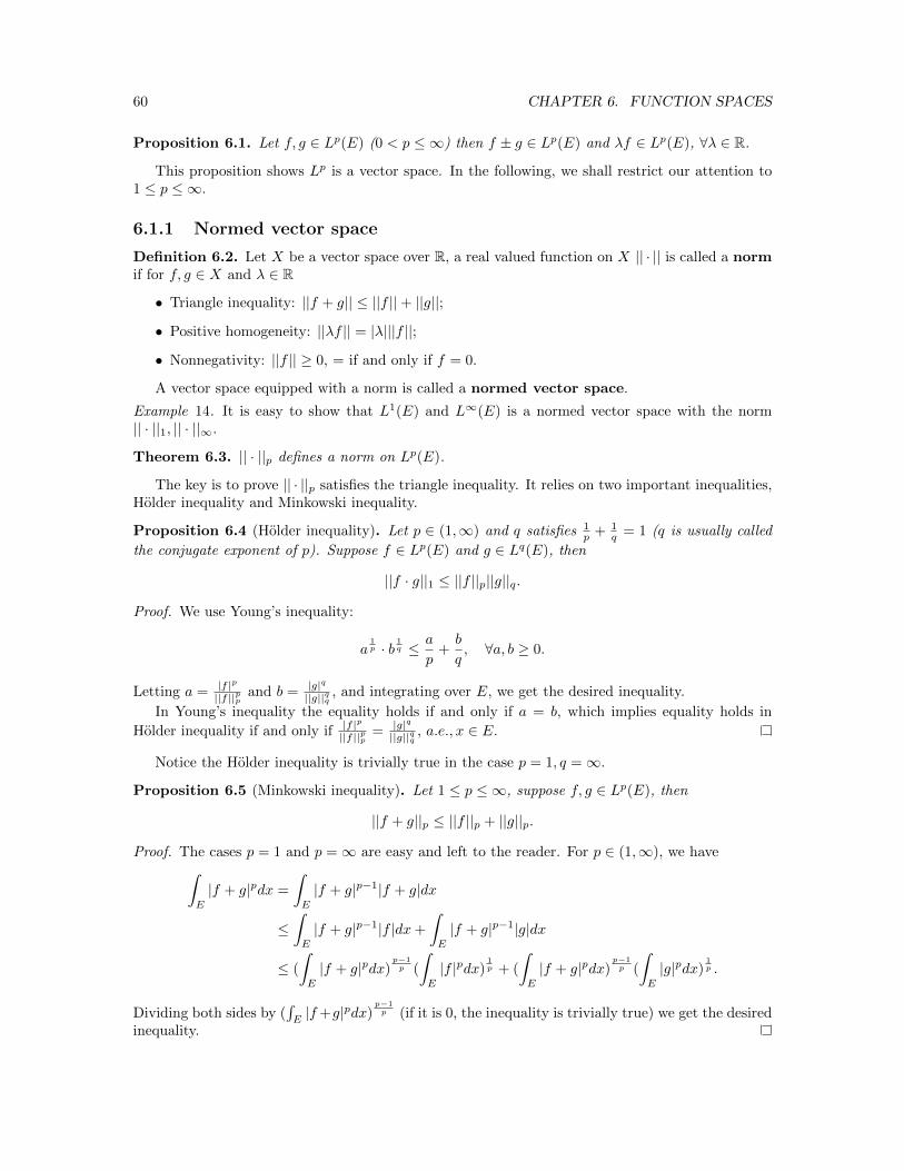
60 CHAPTER 6. FUNCTION SPACES
Proposition 6.1. Let f, g ∈ Lp(E) (0 < p ≤ ∞) then f ± g ∈ Lp(E) and λf ∈ Lp(E), ∀λ ∈ R.
This proposition shows Lp is a vector space. In the following, we shall restrict our attention to1 ≤ p ≤ ∞.
6.1.1 Normed vector space
Definition 6.2. Let X be a vector space over R, a real valued function on X || · || is called a normif for f, g ∈ X and λ ∈ R
• Triangle inequality: ||f + g|| ≤ ||f ||+ ||g||;
• Positive homogeneity: ||λf || = |λ|||f ||;
• Nonnegativity: ||f || ≥ 0, = if and only if f = 0.
A vector space equipped with a norm is called a normed vector space.
Example 14. It is easy to show that L1(E) and L∞(E) is a normed vector space with the norm|| · ||1, || · ||∞.
Theorem 6.3. || · ||p defines a norm on Lp(E).
The key is to prove || · ||p satisfies the triangle inequality. It relies on two important inequalities,Holder inequality and Minkowski inequality.
Proposition 6.4 (Holder inequality). Let p ∈ (1,∞) and q satisfies 1p + 1
q = 1 (q is usually called
the conjugate exponent of p). Suppose f ∈ Lp(E) and g ∈ Lq(E), then
||f · g||1 ≤ ||f ||p||g||q.
Proof. We use Young’s inequality:
a1p · b
1q ≤ a
p+b
q, ∀a, b ≥ 0.
Letting a = |f |p||f ||pp and b = |g|q
||g||qq , and integrating over E, we get the desired inequality.
In Young’s inequality the equality holds if and only if a = b, which implies equality holds in
Holder inequality if and only if |f |p
||f ||pp = |g|q||g||qq , a.e., x ∈ E.
Notice the Holder inequality is trivially true in the case p = 1, q =∞.
Proposition 6.5 (Minkowski inequality). Let 1 ≤ p ≤ ∞, suppose f, g ∈ Lp(E), then
||f + g||p ≤ ||f ||p + ||g||p.
Proof. The cases p = 1 and p =∞ are easy and left to the reader. For p ∈ (1,∞), we have∫E
|f + g|pdx =
∫E
|f + g|p−1|f + g|dx
≤∫E
|f + g|p−1|f |dx+
∫E
|f + g|p−1|g|dx
≤ (
∫E
|f + g|pdx)p−1p (
∫E
|f |pdx)1p + (
∫E
|f + g|pdx)p−1p (
∫E
|g|pdx)1p .
Dividing both sides by (∫E|f+g|pdx)
p−1p (if it is 0, the inequality is trivially true) we get the desired
inequality.
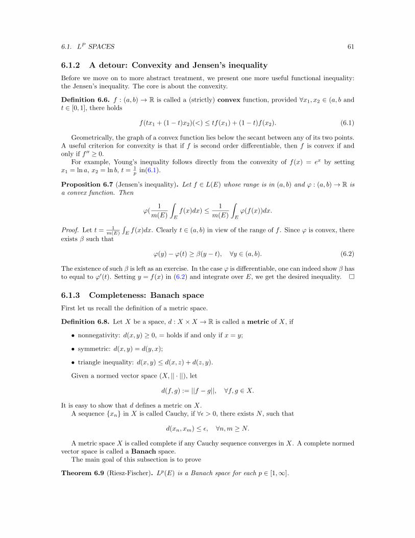
6.1. LP SPACES 61
6.1.2 A detour: Convexity and Jensen’s inequality
Before we move on to more abstract treatment, we present one more useful functional inequality:the Jensen’s inequality. The core is about the convexity.
Definition 6.6. f : (a, b) → R is called a (strictly) convex function, provided ∀x1, x2 ∈ (a, b andt ∈ [0, 1], there holds
f(tx1 + (1− t)x2)(<) ≤ tf(x1) + (1− t)f(x2). (6.1)
Geometrically, the graph of a convex function lies below the secant between any of its two points.A useful criterion for convexity is that if f is second order differentiable, then f is convex if andonly if f ′′ ≥ 0.
For example, Young’s inequality follows directly from the convexity of f(x) = ex by settingx1 = ln a, x2 = ln b, t = 1
p in(6.1).
Proposition 6.7 (Jensen’s inequality). Let f ∈ L(E) whose range is in (a, b) and ϕ : (a, b)→ R isa convex function. Then
ϕ(1
m(E)
∫E
f(x)dx) ≤ 1
m(E)
∫E
ϕ(f(x))dx.
Proof. Let t = 1m(E)
∫Ef(x)dx. Clearly t ∈ (a, b) in view of the range of f . Since ϕ is convex, there
exists β such that
ϕ(y)− ϕ(t) ≥ β(y − t), ∀y ∈ (a, b). (6.2)
The existence of such β is left as an exercise. In the case ϕ is differentiable, one can indeed show β hasto equal to ϕ′(t). Setting y = f(x) in (6.2) and integrate over E, we get the desired inequality.
6.1.3 Completeness: Banach space
First let us recall the definition of a metric space.
Definition 6.8. Let X be a space, d : X ×X → R is called a metric of X, if
• nonnegativity: d(x, y) ≥ 0, = holds if and only if x = y;
• symmetric: d(x, y) = d(y, x);
• triangle inequality: d(x, y) ≤ d(x, z) + d(z, y).
Given a normed vector space (X, || · ||), let
d(f, g) := ||f − g||, ∀f, g ∈ X.
It is easy to show that d defines a metric on X.A sequence xn in X is called Cauchy, if ∀ε > 0, there exists N , such that
d(xn, xm) ≤ ε, ∀n,m ≥ N.
A metric space X is called complete if any Cauchy sequence converges in X. A complete normedvector space is called a Banach space.
The main goal of this subsection is to prove
Theorem 6.9 (Riesz-Fischer). Lp(E) is a Banach space for each p ∈ [1,∞].
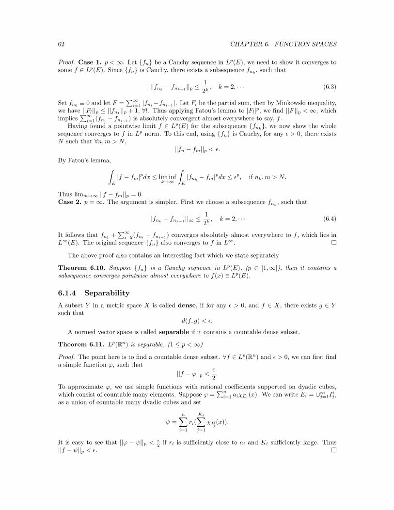
62 CHAPTER 6. FUNCTION SPACES
Proof. Case 1. p <∞. Let fn be a Cauchy sequence in Lp(E), we need to show it converges tosome f ∈ Lp(E). Since fn is Cauchy, there exists a subsequence fnk , such that
||fnk − fnk−1||p ≤
1
2k, k = 2, · · · (6.3)
Set fn0≡ 0 and let F =
∑∞i=1 |fni−fni−1
|. Let Fl be the partial sum, then by Minkowski inequality,we have ||Fl||p ≤ ||fn1
||p + 1, ∀l. Thus applying Fatou’s lemma to |Fl|p, we find ||F ||p < ∞, whichimplies
∑∞i=1(fni − fni−1) is absolutely convergent almost everywhere to say, f .
Having found a pointwise limit f ∈ Lp(E) for the subsequence fnk, we now show the wholesequence converges to f in Lp norm. To this end, using fn is Cauchy, for any ε > 0, there existsN such that ∀n,m > N ,
||fn − fm||p < ε.
By Fatou’s lemma,∫E
|f − fm|pdx ≤ lim infk→∞
∫E
|fnk − fm|pdx ≤ εp, if nk,m > N.
Thus limm→∞ ||f − fm||p = 0.Case 2. p =∞. The argument is simpler. First we choose a subsequence fnk , such that
||fnk − fnk−1||∞ ≤
1
2k, k = 2, · · · (6.4)
It follows that fn1+∑∞i=2(fni − fni−1
) converges absolutely almost everywhere to f , which lies inL∞(E). The original sequence fn also converges to f in L∞.
The above proof also contains an interesting fact which we state separately
Theorem 6.10. Suppose fn is a Cauchy sequence in Lp(E), (p ∈ [1,∞]), then it contains asubsequence converges pointwise almost everywhere to f(x) ∈ Lp(E).
6.1.4 Separability
A subset Y in a metric space X is called dense, if for any ε > 0, and f ∈ X, there exists g ∈ Ysuch that
d(f, g) < ε.
A normed vector space is called separable if it contains a countable dense subset.
Theorem 6.11. Lp(Rn) is separable. (1 ≤ p <∞)
Proof. The point here is to find a countable dense subset. ∀f ∈ Lp(Rn) and ε > 0, we can first finda simple function ϕ, such that
||f − ϕ||p <ε
2.
To approximate ϕ, we use simple functions with rational coefficients supported on dyadic cubes,which consist of countable many elements. Suppose ϕ =
∑ni=1 aiχEi(x). We can write Ei = ∪∞j=1I
ij ,
as a union of countable many dyadic cubes and set
ψ =
n∑i=1
ri(
Ki∑j=1
χIij (x)).
It is easy to see that ||ϕ − ψ||p < ε2 if ri is sufficiently close to ai and Ki sufficiently large. Thus
||f − ψ||p < ε.
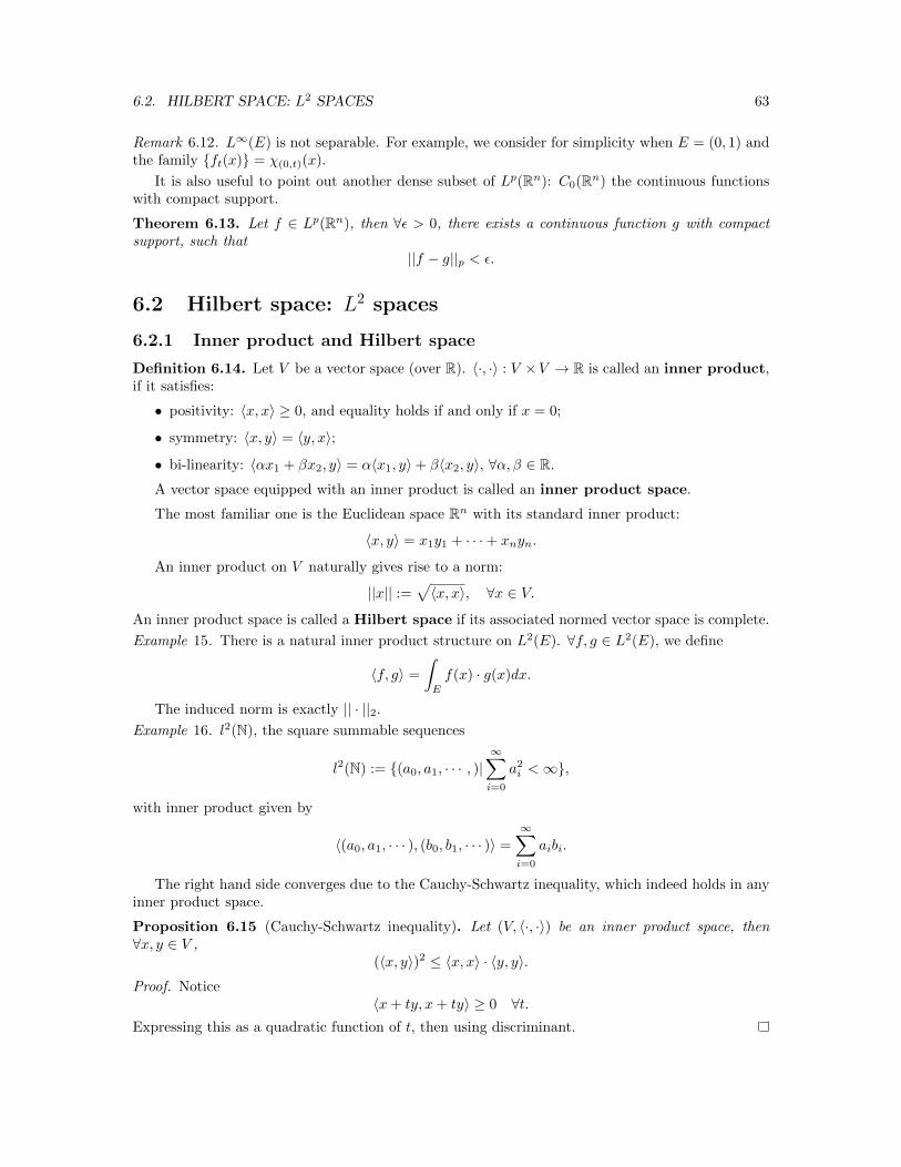
6.2. HILBERT SPACE: L2 SPACES 63
Remark 6.12. L∞(E) is not separable. For example, we consider for simplicity when E = (0, 1) andthe family ft(x) = χ(0,t)(x).
It is also useful to point out another dense subset of Lp(Rn): C0(Rn) the continuous functionswith compact support.
Theorem 6.13. Let f ∈ Lp(Rn), then ∀ε > 0, there exists a continuous function g with compactsupport, such that
||f − g||p < ε.
6.2 Hilbert space: L2 spaces
6.2.1 Inner product and Hilbert space
Definition 6.14. Let V be a vector space (over R). 〈·, ·〉 : V ×V → R is called an inner product,if it satisfies:
• positivity: 〈x, x〉 ≥ 0, and equality holds if and only if x = 0;
• symmetry: 〈x, y〉 = 〈y, x〉;
• bi-linearity: 〈αx1 + βx2, y〉 = α〈x1, y〉+ β〈x2, y〉, ∀α, β ∈ R.
A vector space equipped with an inner product is called an inner product space.
The most familiar one is the Euclidean space Rn with its standard inner product:
〈x, y〉 = x1y1 + · · ·+ xnyn.
An inner product on V naturally gives rise to a norm:
||x|| :=√〈x, x〉, ∀x ∈ V.
An inner product space is called a Hilbert space if its associated normed vector space is complete.
Example 15. There is a natural inner product structure on L2(E). ∀f, g ∈ L2(E), we define
〈f, g〉 =
∫E
f(x) · g(x)dx.
The induced norm is exactly || · ||2.
Example 16. l2(N), the square summable sequences
l2(N) := (a0, a1, · · · , )|∞∑i=0
a2i <∞,
with inner product given by
〈(a0, a1, · · · ), (b0, b1, · · · )〉 =
∞∑i=0
aibi.
The right hand side converges due to the Cauchy-Schwartz inequality, which indeed holds in anyinner product space.
Proposition 6.15 (Cauchy-Schwartz inequality). Let (V, 〈·, ·〉) be an inner product space, then∀x, y ∈ V ,
(〈x, y〉)2 ≤ 〈x, x〉 · 〈y, y〉.Proof. Notice
〈x+ ty, x+ ty〉 ≥ 0 ∀t.Expressing this as a quadratic function of t, then using discriminant.
64 CHAPTER 6. FUNCTION SPACES
6.2.2 Orthogonality, Orthonormal basis, Fourier series
There is a rich geometric content inherited from the inner product. Let H be a Hilbert space, if〈f, g〉 = 0, we call f is orthogonal to g, denoted by f⊥g.
Proposition 6.16 (Pythagorean theorem). Let f, g ∈ H and f⊥g, then ||f + g|| = ||f ||+ ||g||.
Definition 6.17. A finite or countably subset e1, e2, · · · of a Hilbert space H is called orthonor-mal if
〈ei, ej〉 =
1, i = j0, i 6= j.
Theorem 6.18. The following properties of an orthonormal set ei∞i=1 are equivalent.
1. Finite linear combinations of elements in ei are dense in H.
2. If f ∈ H, and f⊥ei, ∀i, then f = 0.
3. Let ai = 〈f, ei〉, SN (f) =∑Ni=1 aiei, then limN→∞ ||SN (f)− f || = 0.
4. (Parseval’s identity) ||f ||2 =∑∞i=1 |ai|2.
Proof. • (1) =⇒ (2). Suppose there exists gn, each as a finite linear combination of ei suchthat limn→∞ ||gn − f || = 0. By assumption 〈f, ei〉 = 0, ∀i, it follows that 〈f, gn〉 = 0, ∀n.Hence by Cauchy Schwartz inequality,
||f ||2 = 〈f, f − gn〉 ≤ ||f ||||f − gn||.
Letting n→∞, we have ||f || = 0, and thus f = 0.
• (2) =⇒ (3). Let ai = 〈f, ei〉, SN (f) =∑Ni=1 aiei. Notice that f − SN (f)⊥SN (f), thus
||f ||2 = ||f − SN (f)||2 + ||SN (f)||2 = ||f − SN (f)||2 +
N∑i=1
a2i . (6.5)
It follows that∞∑i=1
a2i < ||f ||2 <∞,
which is called the Bessel’s inequality. Notice for N ≤M ,
||SN (f)− SM (f)|| =M∑
i=N+1
a2i .
The convergence of∑∞i=1 a
2i thus implies SN (f) is a Cauchy sequence in H. By completeness
of Hilbert space, there exists g ∈ H such that limN→∞ ||SN (f) − g|| = 0. Now for each fixedj,
〈f − SN (f), ej〉 = 0, ∀N > j
it follows that (continuity)〈f − g, ej〉 = 0, ∀j.
Therefore by assumption, we have f = g and thus finish the proof.
• (3) =⇒ (4). Suppose limN→∞ ||SN (f) − f || = 0, then letting N → ∞ in (6.5), we get thedesired equality
||f ||2 =
∞∑i=1
|ai|2.
6.2. HILBERT SPACE: L2 SPACES 65
• (4) =⇒ (1). If ||f ||2 =∑∞i=1 |ai|2 holds, in light of (6.5), it follows limN→∞ ||SN (f)− f || = 0,
therefore f can be approximated by finite linear combination SN (f).
An orthonormal set satisfies one of the above four properties is called an orthonormal basis.
Theorem 6.19. Any separable Hilbert space has an orthonormal basis.
[Sketch of the proof] By separable assumption, we can take a countable set ai which is densein H. We then extract a linearly independent subset, and perform the standard Gram-Schmidtprocess.
An example of an orthonarmal basis for a Hilbert space is the Fourier series theory of L2([−π, π]).More precisely, we consider all square integrable functions on [−π, π], with the inner product
〈f, g〉 =1
2π
∫[−π,π]
f(x) · g(x)dx.
√
2 sin(nx),√
2 cos(nx)∞n=1 is an orthonormal basis. We shall explore this fact in Chapter 7.
6.2.3 Linear functional, Duality
By a closed subspace of H, we mean a subspace in the sense of vector space which is closed underthe metric topology induced by the inner product. Denote by x⊥ the set of all y ∈ H, such thatx⊥y. It can be shown that x⊥ is a closed subspace of H. Let
K⊥ =⋂x∈M
x⊥.
K⊥ is an intersection of closed subspace, and thus a closed subspace of H as well.
Theorem 6.20. Let K be a closed subspace of H.
• ∀f ∈ H has a unique decomposition
f = P (f) +Q(f),
where P (f) ∈M and Q(f) ∈M⊥.
• P (f) and Q(f) are nearest point to f in K and K⊥ respectively.
• ||f ||2 = ||P (f)||2 + ||Q(f)||2.
Proof. ConsiderD(g) := ||f − g||2, g ∈ K.
Let D0 = infg∈K D(g). Then there exists a sequence gi ∈ K such that
||f − gi||2 → D0. (6.6)
We claim gi is a Cauchy sequence. Recall so called parallelogram law:
||x− y||2 + ||x+ y||2 = 2(||x||2 + ||y||2).
Letting x = f−gi2 and y =
f−gj2 , we get
1
4||gi − gj ||2 =
1
2(||f − gi||2 + ||f − gj ||2)− ||f − gi + gi
2|| ≤ 1
2(||f − gi||2 + ||f − gj ||2)−D0.
(6.7)
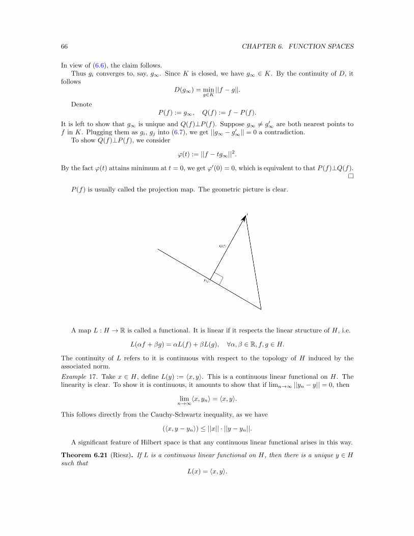
66 CHAPTER 6. FUNCTION SPACES
In view of (6.6), the claim follows.Thus gi converges to, say, g∞. Since K is closed, we have g∞ ∈ K. By the continuity of D, it
followsD(g∞) = min
g∈K||f − g||.
DenoteP (f) := g∞, Q(f) := f − P (f).
It is left to show that g∞ is unique and Q(f)⊥P (f). Suppose g∞ 6= g′∞ are both nearest points tof in K. Plugging them as gi, gj into (6.7), we get ||g∞ − g′∞|| = 0 a contradiction.
To show Q(f)⊥P (f), we consider
ϕ(t) := ||f − tg∞||2.
By the fact ϕ(t) attains minimum at t = 0, we get ϕ′(0) = 0, which is equivalent to that P (f)⊥Q(f).
P (f) is usually called the projection map. The geometric picture is clear.
A map L : H → R is called a functional. It is linear if it respects the linear structure of H, i.e.
L(αf + βg) = αL(f) + βL(g), ∀α, β ∈ R, f, g ∈ H.
The continuity of L refers to it is continuous with respect to the topology of H induced by theassociated norm.
Example 17. Take x ∈ H, define L(y) := 〈x, y〉. This is a continuous linear functional on H. Thelinearity is clear. To show it is continuous, it amounts to show that if limn→∞ ||yn − y|| = 0, then
limn→∞
〈x, yn〉 = 〈x, y〉.
This follows directly from the Cauchy-Schwartz inequality, as we have
(〈x, y − yn〉) ≤ ||x|| · ||y − yn||.
A significant feature of Hilbert space is that any continuous linear functional arises in this way.
Theorem 6.21 (Riesz). If L is a continuous linear functional on H, then there is a unique y ∈ Hsuch that
L(x) = 〈x, y〉.
6.2. HILBERT SPACE: L2 SPACES 67
Proof. If L(x) ≡ 0, then y = 0 furnishes the requirement. Otherwise, let
K = x : L(x) = 0.
Linearity of L implies K is a subspace and continuity shows that K is closed. Hence there existsz ∈ K⊥, with ||z|| = 1. Put
u = L(x)z − L(z)x.
Direct computation shows that L(u) = 0, thus u⊥z. We get
L(x) = L(x)||z||2 = L(z)〈x, z〉, ∀x ∈ H.
Set y = L(z)z, we get the desired y, such that
L(x) = 〈x, y〉.
Uniqueness of such y is easy. Suppose there are y and y′ such that
〈x, y〉 = 〈x, y′〉, ∀x ∈ H.
Therefore 〈x, y − y′〉 = 0, ∀x. Set x = y − y′, it follows that y = y′.

68 CHAPTER 6. FUNCTION SPACES
Chapter 7
Fourier Series
#à[1˶§´c3v/K"ìYE¦Ã´§7Vs²q~"
))ºi5iìÜ~6
Starting with this Chapter, we begin to touch the second part of this course: Fourier analysis. In thissection, we introduce the basic definition of the Fourier series, and the main issue we address hereis the various convergence results for Fourier series. We end the section with several applications,from which the reader may feel the wideness of the application of the Fourier series. In the nextsection, we study Fourier transform, which can be viewed as a continuous version of Fourier series.We also conclude the section with various application. In the last section, we study selected topicswhich are further deep application of Fourier analysis.
7.1 Introduction
Let f(x) be an integrable (Lebesgue) function defined on [−π, π], with f(−π) = f(π). Sometimes itis regarded as a function of period 2π on R, or equivalently a function defined on the unit circle.
Set
an =1
2π
∫ π
−πf(x)e−inxdx,
then the series∞∑
n=−∞ane
inx
is called the Fourier series of f . We denote the partial sum as
SN (f)(x) =
N∑n=−N
aneinx.
The main question is in what sense SN (f) converges to f? Before answering this question in details,we first look at some examples.
Example 18.
69
70 CHAPTER 7. FOURIER SERIES
7.2 Pointwise convergence
We shall derive a localization property of the convergence of the Fourier series. Let f be an integrablefunction of 2π-period. Then
(7.1)
SN (f)(x) =
N∑n=−N
aneinx
=
N∑n=−N
(1
2π
∫ π
−πf(y)e−inydy
)einx
=
N∑n=−N
1
2π
∫ π
−πf(y)ein(x−y)dy. (7.2)
Theorem 7.1 (Localization property). Suppose f is an integrable function of period 2π and it isdifferentiable at x0, then
limN→∞
SN (f)(x0) = f(x0).
A second thought on this conclusion: even though the Fourier coeffients depend on the the wholevalue of f over a period, the convergence at a single point only depends on the local behavior of f .We recall the Riemann-Lebesgue lemma in Chapter.
Proof. Noticing that 12π
∫ π−πDN (f)(y)dy = 1, we have
SN (f)(x0)− f(x0) =1
2π
∫ π
−π[f(x0 − y)− f(x0)]
(N∑
n=−Neiny
)dy. (7.3)
A simple sum for the geometric series∑Nn=−N e
iny yields that
N∑n=−N
einy =sin( 2N+1
2 y)
sin( 12y)
.
By the assumption that f is differentiable at x0, we infer that
F (y) =f(x0 − y)− f(x0)
y
is integrable on [−π, π]. Hence the integrand in (7.3) can be written as
[f(x0 − y)− f(x0)]
(N∑
n=−Neiny
)= F (y) · y
sin(y2 )· sin(
2N + 1
2y).
The conclusion then follows in view of the Riemann-Lebesgue lemma.
Next we shall write (7.2) as a convolution
SN (f)(x) = (f ∗DN )(x),
where DN =∑Nn=−N e
inx is called the N -th Dirichlet kernel. Using the property of good kernels,we are able to show two interesting convergence theory for Fourier series.
A family of functions Kn(x) defined on unit circle is said to be a good kernels if it satisfies
7.2. POINTWISE CONVERGENCE 71
1. For all n ≥ 1,1
2π
∫ π
−πKn(x)dx = 1.
2. There exists M > 0 such that for all n ≥ 1,∫ π
−π|Kn(x)|dx ≤M.
3. For every δ > 0,
limN→∞
∫δ≤|x|≤π
|Kn(x)|dx = 0.
We have
Theorem 7.2. Let Kn(x) be a family of good kernels, and f a bounded integrable function on thecircle. Then
limn→∞
(f ∗Kn)(x) = f(x),
whenever f is continuous at x. Moreover, if f is continuous everywhere, then the above limit isuniform.
Proof. Suppose |f(x)| ≤ B, and let x be a point of continuity of f . Then ∀ε > 0, ∃δ > 0 such that
|f(x− y)− f(x)| ≤ ε,whenever|y| < δ.
We have
|Kn ∗ f(x)− f(x)| ≤ 1
2π
∫ π
−π|Kn(y)||f(x− y)− f(x)|dy (7.4)
≤ 1
2π
∫|y|<δ
|Kn(y)||f(x− y)− f(x)|dy +1
2π
∫δ≤|x|≤π
|Kn(y)||f(x− y)− f(x)|dy
≤ ε 1
2π
∫|y|<δ
|Kn(y)|dy + 2B1
2π
∫δ≤|x|≤π
|Kn(y)|dy.
The condition (2) of good kernels implies ε 12π
∫|y|<δ |Kn(y)|dy ≤ Mε. The condition (3) of good
kernels implies there exists N such that for all n ≥ N , 2B 12π
∫δ≤|x|≤π |Kn(y)|dy ≤ ε. In all
limn→∞
(f ∗Kn)(x) = f(x).
If f is continuous everywhere, then f is uniformly continuous. The above choice of δ is indepen-dent of x and thus the convergence is uniform.
Sometimes Kn(x) is referred to as an approximation to the identity.
7.2.1 Cesaro summation
For a series∑∞n=1 an, its partial sum is
sn = a1 + · · ·+ an.
The N -th Cesaro mean is
σN =s1 + s2 + · · ·+ sN
N.
The series∑∞n=1 an is called Cesaro summable if limN→∞ σN exits. Applying Theorem 7.2, we shall
show
72 CHAPTER 7. FOURIER SERIES
Theorem 7.3. If f is integrable on the circle, then then Fourier series of f is Cesaro summableto f at every point of continuity of f . Moreover, if f is continuous on the circle, then the Fourierseries is uniformly Cesaro summable to f .
A nice consequence is
Corollary 7.4. Any continuous function f on the circle can be uniformly approximated by trigono-metric polynomials.
Proof of Theorem 7.3. In view of Theorem 7.2, we just need to show the kernels for Cesaro sum isa family of good kernels. Since SN (f) = (f ∗DN ), then
σN (f) =S1(f) + S2(f) + · · ·+ SN (f)
N= (f ∗ FN )(x),
where FN is given by
FN =D1 +D2 + · · ·+DN
N.
A simple calculation shows
FN =1
N
sin2(Nx2 )
sin2(x2 ).
We leave as an exercise to the reader to verify that FN is a family of good kernels.
7.2.2 Abel summation
A series of complex numbers∑∞n=1 an is called Able summable to s if A(r) =
∑∞n=1 anr
n convergesfor 0 ≤ r < 1 and
limr→1
A(r) = s
exists. A(r) is called the Abel means of the series.Given a Fourier series f(θ) ∼
∑∞n=−∞ ane
inθ, its Abel means are given by
Ar(f)(θ) =
∞∑n=−∞
r|n|aneinθ.
Set Pr(θ) =∑∞n=−∞ r|n|e∈θ, which is called the Poisson kernel, we find that
Ar(f)(θ) = (f ∗ Pr)(θ).
For 0 ≤ r < 1, a simple calculation shows that
Pr(θ) =1− r2
1− 2r cos θ + r2.
We leave as an exercise to the reader to show that Pr(θ) is a family of good kernels as r approachesto 1 from below. Hence we have
Theorem 7.5. The Fourier series of f is Abel summable to f at its points of continuity. Moreover,if f is continuous, then the Abel summation is uniform.
As an application, we can solve Dirichlet problem for harmonic functions on unit disk.
Theorem 7.6. Suppose u ∈ C2(B1) ∩ C(B1) is the solution to the Dirichlet problem∆u(x) = 0, x ∈ B1
u = f, on∂B1.
Then u(r, θ) = (f ∗ Pr)(θ).
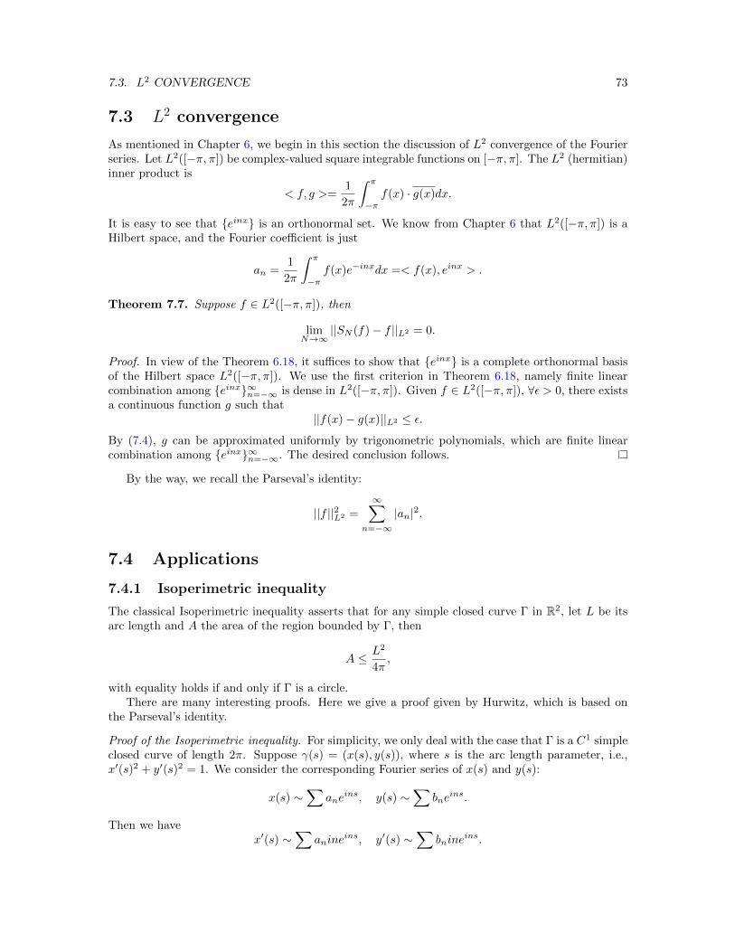
7.3. L2 CONVERGENCE 73
7.3 L2 convergence
As mentioned in Chapter 6, we begin in this section the discussion of L2 convergence of the Fourierseries. Let L2([−π, π]) be complex-valued square integrable functions on [−π, π]. The L2 (hermitian)inner product is
< f, g >=1
2π
∫ π
−πf(x) · g(x)dx.
It is easy to see that einx is an orthonormal set. We know from Chapter 6 that L2([−π, π]) is aHilbert space, and the Fourier coefficient is just
an =1
2π
∫ π
−πf(x)e−inxdx =< f(x), einx > .
Theorem 7.7. Suppose f ∈ L2([−π, π]), then
limN→∞
||SN (f)− f ||L2 = 0.
Proof. In view of the Theorem 6.18, it suffices to show that einx is a complete orthonormal basisof the Hilbert space L2([−π, π]). We use the first criterion in Theorem 6.18, namely finite linearcombination among einx∞n=−∞ is dense in L2([−π, π]). Given f ∈ L2([−π, π]), ∀ε > 0, there existsa continuous function g such that
||f(x)− g(x)||L2 ≤ ε.
By (7.4), g can be approximated uniformly by trigonometric polynomials, which are finite linearcombination among einx∞n=−∞. The desired conclusion follows.
By the way, we recall the Parseval’s identity:
||f ||2L2 =
∞∑n=−∞
|an|2.
7.4 Applications
7.4.1 Isoperimetric inequality
The classical Isoperimetric inequality asserts that for any simple closed curve Γ in R2, let L be itsarc length and A the area of the region bounded by Γ, then
A ≤ L2
4π,
with equality holds if and only if Γ is a circle.There are many interesting proofs. Here we give a proof given by Hurwitz, which is based on
the Parseval’s identity.
Proof of the Isoperimetric inequality. For simplicity, we only deal with the case that Γ is a C1 simpleclosed curve of length 2π. Suppose γ(s) = (x(s), y(s)), where s is the arc length parameter, i.e.,x′(s)2 + y′(s)2 = 1. We consider the corresponding Fourier series of x(s) and y(s):
x(s) ∼∑
aneins, y(s) ∼
∑bne
ins.
Then we havex′(s) ∼
∑anine
ins, y′(s) ∼∑
bnineins.
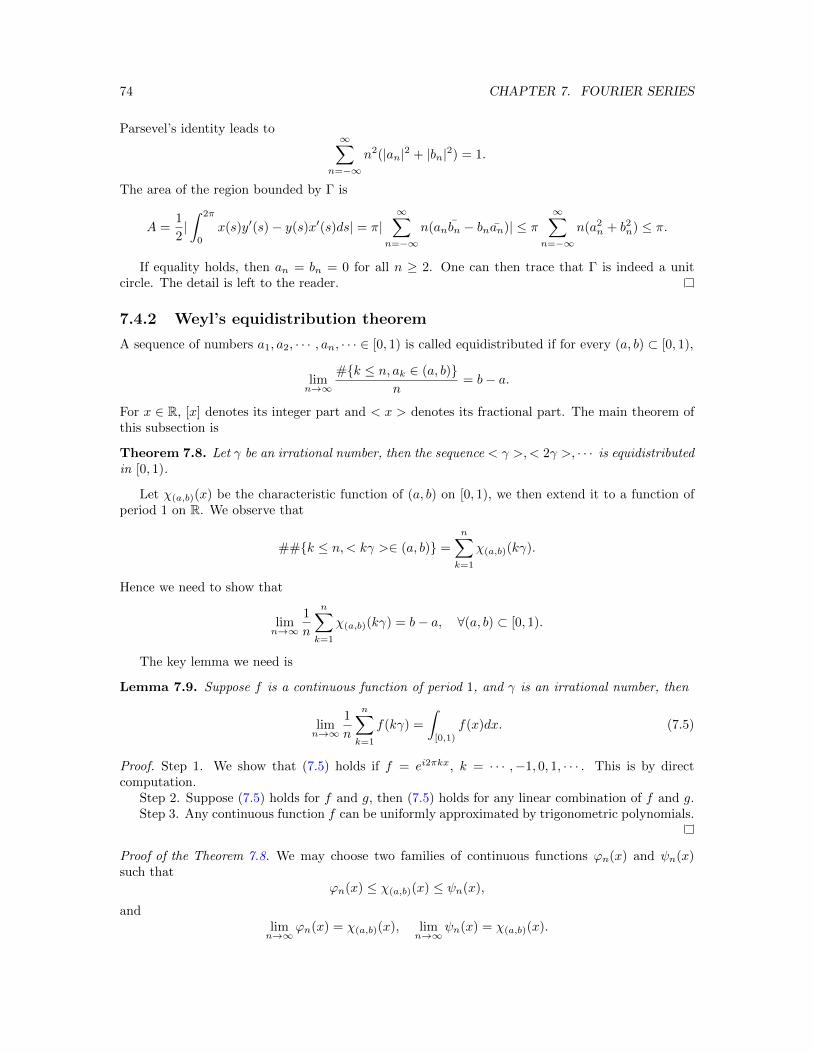
74 CHAPTER 7. FOURIER SERIES
Parsevel’s identity leads to∞∑
n=−∞n2(|an|2 + |bn|2) = 1.
The area of the region bounded by Γ is
A =1
2|∫ 2π
0
x(s)y′(s)− y(s)x′(s)ds| = π|∞∑
n=−∞n(anbn − bnan)| ≤ π
∞∑n=−∞
n(a2n + b2n) ≤ π.
If equality holds, then an = bn = 0 for all n ≥ 2. One can then trace that Γ is indeed a unitcircle. The detail is left to the reader.
7.4.2 Weyl’s equidistribution theorem
A sequence of numbers a1, a2, · · · , an, · · · ∈ [0, 1) is called equidistributed if for every (a, b) ⊂ [0, 1),
limn→∞
#k ≤ n, ak ∈ (a, b)n
= b− a.
For x ∈ R, [x] denotes its integer part and < x > denotes its fractional part. The main theorem ofthis subsection is
Theorem 7.8. Let γ be an irrational number, then the sequence < γ >,< 2γ >, · · · is equidistributedin [0, 1).
Let χ(a,b)(x) be the characteristic function of (a, b) on [0, 1), we then extend it to a function ofperiod 1 on R. We observe that
##k ≤ n,< kγ >∈ (a, b) =
n∑k=1
χ(a,b)(kγ).
Hence we need to show that
limn→∞
1
n
n∑k=1
χ(a,b)(kγ) = b− a, ∀(a, b) ⊂ [0, 1).
The key lemma we need is
Lemma 7.9. Suppose f is a continuous function of period 1, and γ is an irrational number, then
limn→∞
1
n
n∑k=1
f(kγ) =
∫[0,1)
f(x)dx. (7.5)
Proof. Step 1. We show that (7.5) holds if f = ei2πkx, k = · · · ,−1, 0, 1, · · · . This is by directcomputation.
Step 2. Suppose (7.5) holds for f and g, then (7.5) holds for any linear combination of f and g.Step 3. Any continuous function f can be uniformly approximated by trigonometric polynomials.
Proof of the Theorem 7.8. We may choose two families of continuous functions ϕn(x) and ψn(x)such that
ϕn(x) ≤ χ(a,b)(x) ≤ ψn(x),
andlimn→∞
ϕn(x) = χ(a,b)(x), limn→∞
ψn(x) = χ(a,b)(x).
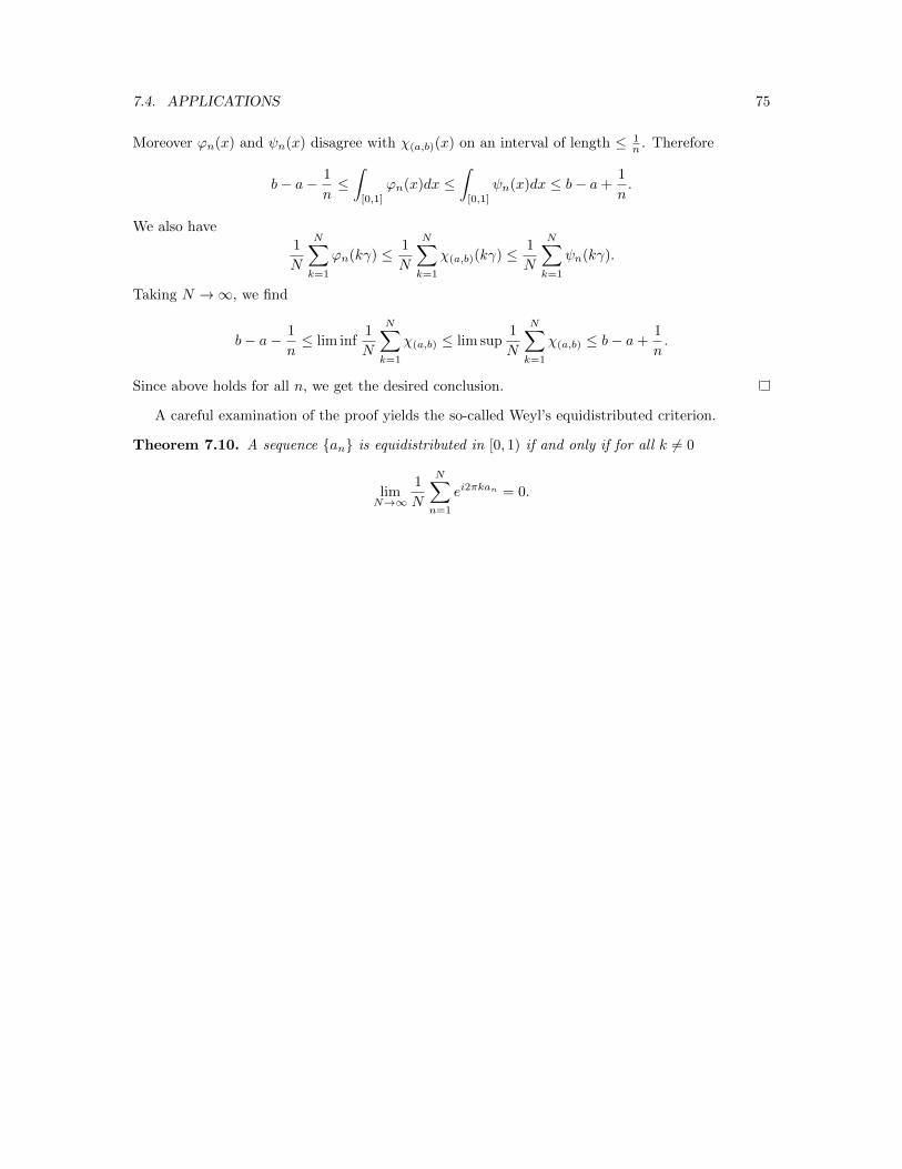
7.4. APPLICATIONS 75
Moreover ϕn(x) and ψn(x) disagree with χ(a,b)(x) on an interval of length ≤ 1n . Therefore
b− a− 1
n≤∫
[0,1]
ϕn(x)dx ≤∫
[0,1]
ψn(x)dx ≤ b− a+1
n.
We also have
1
N
N∑k=1
ϕn(kγ) ≤ 1
N
N∑k=1
χ(a,b)(kγ) ≤ 1
N
N∑k=1
ψn(kγ).
Taking N →∞, we find
b− a− 1
n≤ lim inf
1
N
N∑k=1
χ(a,b) ≤ lim sup1
N
N∑k=1
χ(a,b) ≤ b− a+1
n.
Since above holds for all n, we get the desired conclusion.
A careful examination of the proof yields the so-called Weyl’s equidistributed criterion.
Theorem 7.10. A sequence an is equidistributed in [0, 1) if and only if for all k 6= 0
limN→∞
1
N
N∑n=1
ei2πkan = 0.

76 CHAPTER 7. FOURIER SERIES
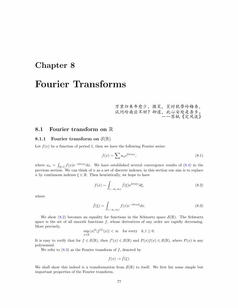
Chapter 8
Fourier Transforms
p85c§§g*r§Á¯*HAØк%§d%S?´Æ"
))ç5½ºÅ6
8.1 Fourier transform on R8.1.1 Fourier transform on S(R)Let f(x) be a function of period 1, then we have the following Fourier series:
f(x) ∼∑
ane2πinx, (8.1)
where an =∫
[0,1]f(x)e−2πinxdx. We have established several convergence results of (8.4) in the
previous section. We can think of n as a set of discrete indexes, in this section our aim is to replacen by continuous indexes ξ ∈ R. Then heuristically, we hope to have
f(x) ∼∫
(−∞,∞)
f(ξ)e2πiξxdξ, (8.2)
where
f(ξ) =
∫(−∞,∞)
f(x)e−2πixξdx. (8.3)
We show (8.2) becomes an equality for functions in the Schwartz space S(R). The Schwartzspace is the set of all smooth functions f , whose derivatives of any order are rapidly decreasing.More precisely,
supx∈R|x|k|f (l)(x)| <∞ for every k, l ≥ 0.
It is easy to verify that for f ∈ S(R), then f ′(x) ∈ S(R) and P (x)f(x) ∈ S(R), where P (x) is anypolynomial.
We refer to (8.3) as the Fourier transform of f , denoted by
f(x)→ f(ξ).
We shall show this indeed is a transformation from S(R) to itself. We first list some simple butimportant properties of the Fourier transform.
77
78 CHAPTER 8. FOURIER TRANSFORMS
Proposition 8.1. If f ∈ S(R), then
1. f(x+ h)→ f(ξ)e2πihξ whenever h ∈ R,
2. f(x)e−2πixh → f(ξ + h) whenever h ∈ R,
3. f(δx)→ δ−1f(δ−1ξ) whenever δ > 0,
4. f ′(x)→ 2πiξf(ξ),
5. −2πixf(x)→ ddξ f(ξ).
Proof. The first three properties concern the behavior of Fourier transform with respect to trans-lation and dilation, which follow directly from the definition. For (4), via integration by parts wehave ∫
(−∞,∞)
f ′(x)e−2πixξdx = 2πiξ
∫(−∞,∞)
f(x)e−2πiξxdx = 2πiξf(ξ).
For (5), since f ∈ S(R), by dominated convergence theorem, one can interchange the derivative withthe integral, i.e.,
d
dξ
∫(−∞,∞)
f(x)e−2πixξdx =
∫(−∞,∞)
∂
∂ξ(f(x)e−2πixξ)dx =
∫(−∞,∞)
−2πixf(x)e−2πixξdx.
Based on properties (4) and (5), Fourier transform interchanges the differentiation and multipli-
cation with −2πix. Using this, we can show f is also rapidly decreasing if f is.
Theorem 8.2. If f ∈ S(R), then f ∈ S(R).
Proof. First of all, notice if f ∈ S(R), then f is bounded. Next, the function
ξk(f)(l)(ξ)
is indeed the Fourier transform of
1
(2πi)k[(−2πix)lf(x)](k),
which is rapidly decreasing. Hence ξk(f)(l)(ξ) is bounded for all k, l ≥ 0, i.e., f ∈ S(R).
8.1.2 Inversion formula
In this subsection, we prove the inversion formula.
Theorem 8.3 (Fourier inversion). If f ∈ S(R), then
f(x) =
∫(−∞,∞)
f(ξ)e2πixξdξ.
To begin with, we show the Gaussian yields a family of good kernels.
Proposition 8.4. If f(x) = e−πx2
, then f(ξ) = e−πξ2
.
8.1. FOURIER TRANSFORM ON R 79
Proof. Let
F (ξ) = f(ξ) =
∫(−∞,∞)
f(x)e−2πixξdx.
First note that F (0) = 1, and then we have
F ′(ξ) =
∫(−∞,∞)
−2πixf(x)e−2πixξdx
= i
∫(−∞,∞)
f ′(x)e−2πixξdx
= −2πξ
∫(−∞,∞)
f(x)e−2πixξdx = −2πξF (ξ).
Therefore F (ξ) = e−πξ2
.
Corollary 8.5. If δ > 0 and Kδ(x) = δ−12 e−πx
2/δ, then Kδ(ξ) = e−πδξ2
.
Proposition 8.6. Kδδ>0 is a family of good kernels as δ → 0.
Proof. We need to verify
1.∫
(−∞,∞)Kδ(x)dx = 1, ∀δ > 0,
2.∫
(−∞,∞)|Kδ(x)|dx ≤M ,
3. For every η > 0, limδ→0
∫|x|>η |Kδ(x)|dx = 0.
We leave as exercises to the reader.
Consequently, we have
Proposition 8.7. If f ∈ S(R), then
limδ→0
(f ∗Kδ)(x) = f(x).
The convergence is uniform in x.
Proposition 8.8 (multiplication formula). If f, g ∈ S(R), then∫(−∞,∞)
f(x)g(x)dx =
∫(−∞,∞)
f(x)g(x)dx.
Proof. Writing out f and f by definition, one sees that the desired identity follows from the Fubini’stheorem.
Now we are in position to prove the inversion formula.
Proof of Theorem 8.3. First we claim that
f(0) =
∫(−∞,∞)
f(ξ)dξ.
Indeed, let Gδ(x) = e−πδx2
, then Gδ = Kδ. By multiplication formula∫(−∞,∞)
f(x)Gδ(x)dx =
∫(−∞,∞)
f(x)Kδ(x)dx =
∫(−∞,∞)
f(x)Gδ(x)dx.
80 CHAPTER 8. FOURIER TRANSFORMS
Since Kδ(x) is a family of good kernels, by letting δ → 0, the left hand side of above converges tof(0). On the other hand, by the dominate convergence theorem, the right hand side of the above
converges to∫
(−∞,∞)f(x)dx.
In general, let F (y) = f(x+ y), then
f(x) = F (0) =
∫(−∞,∞)
F (ξ)dξ =
∫(−∞,∞)
f(ξ)e2πiξxdξ.
8.1.3 The Plancherel formula
From the previous sections, the Fourier transform can be viewed a continuous version of the Fourierseries. What the inversion formula concerns is similar to the pointwise convergence of the Fourierseries. In this section, we prove the Plancherel formula, which is analogous to the L2-convergenceof the Fourier series or more precisely the Parseval’s identity.
We first establish the following properties regarding the convolution and Fourier transform.
Proposition 8.9. If f, g ∈ S(R), then
1. f ∗ g ∈ S(R),
2. f ∗ g = g ∗ f ,
3. (f ∗ g)(ξ) = f(ξ)g(ξ).
Proof. We leave the first two properties as exercise to the reader. For (3), we have by Fubini’stheorem that
f ∗ g(ξ) =
∫ (∫f(x− y)g(y)dy
)e−2πixξdx
=
∫f(x− y)e−2πi(x−y)ξdx
∫g(y)e−2πiyξdy = f(ξ)g(ξ).
Equip S(R) with the following hermitian inner product
(f, g) =
∫(−∞,∞)
f(x)g(x)dx,
then its associated norm is
||f || =
(∫(−∞,∞)
|f(x)|2) 1
2
.
The analogous Parseval’s identity for Fourier transform on S(R) is
Theorem 8.10 (Plancherel). If f ∈ S(R) then ||f || = ||f ||.
Proof. Set g(x) = f(−x), it follows that g(ξ) = f(ξ). Consider h = f ∗ g, then by the third propertyof Proposition 8.9 we have
h(ξ) = f(ξ) · g(ξ) = |f(x)|2. (8.4)
8.2. FOURIER TRANSFORM ON RN 81
By definition of the convolution,
h(0) =
∫(−∞,∞)
f(x)g(−x)dx =
∫(−∞,∞)
|f(x)|2dx.
Using the inversion formula, we also have
h(0) =
∫(−∞,∞)
h(ξ)dξ,
plugging (8.4) back to the above, we obtain∫(−∞,∞)
|f(x)|2dx =
∫(−∞,∞)
|f(ξ)|2dξ.
Remark 8.11. For simplicity,our treatment here for Fourier transform is restricted to the Schwartzspace. Many results can be generalized to more general function space, say L1(R). Indeed, theFourier transform (8.3) makes sense provided f ∈ L1(R), and by dominated convergence theorem
it follows that f is continuous and bounded. Furthermore, if f ∈ L1(Rn), then we also have theinversion formula, i.e.,
f(x) =
∫(−∞,∞)
f(ξ)e2πiξxdξ.
Notice that in general (8.3) does not make sense if f ∈ L2(R). However, using the Plancherelformula, one is able to extend the Fourier transform to L2(R). The idea is as follows. The Plancherelformula asserts that the Fourier transform is an L2 isometry from S(R)→ S(R). Since S(R) is densein L2(R), thus we can extend by continuity the Fourier transform to an isometry on L2(R).
8.2 Fourier transform on Rn
In this section, we discuss the Fourier transform on Rn. With the familiarity with the Fouriertransform on R, our discussion shall be brief. Both inversion formula and Plancherel formula hold.
Let α = (α1, · · · , αn) denote a multi-index. The monomial xα is short for
xα11 xα2
2 · · ·xαnn ,
and similarly ( ∂∂x )α stands for
(∂
∂x1)α1 · · · ( ∂n
∂xn)αn .
The Schwartz space S(Rn) consists of all smooth functions such that
supx∈Rn
|xα(∂
∂x)β | <∞.
The Fourier transform on f ∈ S(Rn) is given by
f(ξ) =
∫Rnf(x)e−2πix·ξdx, ξ ∈ Rn. (8.5)
We use f → f denote the transformation. We list below the basic properties of the Fouriertransform.
82 CHAPTER 8. FOURIER TRANSFORMS
Proposition 8.12. Let f ∈ S(Rn), then
1. f(x+ h)→ f(ξ)e2πiξ·h, ∀h ∈ Rn,
2. f(x)e−2πix·h → f(ξ + h), ∀h ∈ Rn,
3. f(δx)→ δ−nf(δ−1ξ), δ > 0,
4. ( ∂∂x )αf(x)→ (2πiξ)αf(ξ),
5. (−2πix)αf(x)→ ( ∂∂ξ )αf(ξ),
6. f(Ax)→ f(Ax) where A is an orthogonal matrix.
Properties (4) and (5) imply that Fourier transform maps S(Rn) to itself. The following theoremis the inversion formula and Plancherel theorem for Fourier transform in S(Rn).
Theorem 8.13. Suppose f ∈ S(Rn). Then
f(x) =
∫Rnf(ξ)e2πiξ·xdξ,
and ∫Rn|f(ξ)|2dξ =
∫Rn|f(x)|2dx.
Proof. Step 1. The Fourier transform of e−π|x|2
is e−π|ξ|2
.Step 2. The family Kδ(x) = δ−
n2 e−π|x|
2/δ is a family of good kernels.Step 3. The multiplication formula∫
Rnf(x)g(x)dx =
∫Rnf(x)g(x)dx
holds.Step 4. The inversion formula is a simple consequence of the multiplication formula and the
family of good kernels Kδ.Step 5. For f, g ∈ S(Rn), recall the convolution
(f ∗ g)(x) =
∫Rnf(y)g(x− y)dy.
Then we havef ∗ g(ξ) = f(ξ)g(ξ).
Argue similarly as in Theorem 8.10, we obtain the Plancherel formula for Fourier transform inS(Rn).
8.3 Applications
In this section, we discuss some application of Fourier transform to partial differential equations.
8.3.1 Heat equation on R
8.3.2 Harmonic functions on upper half plane
8.3.3 Wave equation in Rn × R

Chapter 9
Selected topics
U¥äÙôm§+YÀ6d£"üWìéѧ~¡F>5"
))ox5"Uì6
In this chapter, we present several interesting applications of Fourier transform.
9.1 Dirichlet Theorem
In this section, we introduce Dirichlet’s theorem on primes in arithmetic progression. It is relatedto Fourier series on finite group. For simplicity, most of proofs are omitted and we refer the readerto Stein’s book for details. We attempt to make the whole strategy clear.
The story begins with Euclid’s proof of the infinitude of primes.
Theorem 9.1. There are infinitely many primes.
Proof. Suppose there are only finitely many primes, say p1, · · · , pn. Consider the number
N = p1 · p2 · · · pn + 1.
Then N must be a composite number. Since every composite integer can be factored uniquely intoa product of primes, so there must exists a prime factor of N , say q which is not one of p1, · · · pn, acontradiction.
The above argument is elegant and ingenious. We can make a twist of it to show there areinfinitely many primes in the form of 4k + 3. Suppose there are only finitely many primes of theform 4k + 3, say p1, · · · , pn. Consider the number
N = 4p1p2 · · · pn + 3.
Then it must be a composite number. Its prime factors cannot be p1, · · · , pn and 3. Moreover, primefactors of N cannot be all of the form 4k + 1, since the product of 4k + 1 is still 4k + 1. Thereforethere exists a prime factor of the form 4k + 3, which is not one of p1, · · · , pn, a contradiction.
However, such argument cann’t be used to show there are infinitely many primes of the form4k + 1. Legendre formulated the following question: suppose l, q are coprime, are there infinitelymany primes in the arithmetic progression
l + kq, k = 0, 1, 2, · · ·?
This was answered affirmatively by Dirichlet.
83
84 CHAPTER 9. SELECTED TOPICS
Theorem 9.2 (Dirichlet). If l, q are coprime, then there are infinitely many primes of the forml + kq.
At the first sight of the question, one hardly sees any connection with the Fourier series. In orderto show there are infinitely many primes in l + kq, the idea is to look at the series∑
p≡l mod q
1
ps, (9.1)
where the sum is over all primes congruent to l modulo q. The divergence of (9.1) would certainlyimply the infinitude of primes in the form of l + kq.
To study the series (9.1), we digress into the Fourier analysis on finite group.
9.1.1 Fourier analysis on finite group
Let G be a finite Abelian group. A character is a homomorphism χ : G→ S1, where S1 is identifiedwith the multiplicative group of unit complex numbers. Let V be the vector space of complex-valuedfunctions on G. It is isomorphic to C|G|. We define a Hermitian inner product on V as follows:
(f, g) =1
|G|∑a∈G
f(a)g(a).
Theorem 9.3. The characters of G form an orthonormal basis of V , which is denoted by G.
The expression of f ∈ V as a linear combination of characters can be viewed as a Fourier series,namely
f =∑e∈G
cee, (9.2)
where ce = (f, e).
Example 19. Let Z(p) be the group of the equivalent classes of all integers modulo p, i.e. Z(p) =0, 1, · · · , p − 1. Z(p) is an Abelian group under addition. Moreover, multiplication also makessense. An element m is called a unit, if there exists k ∈ Z, such that
km ≡ 1 mod p.
The collection of all units in Z(p) is denoted by Z∗(p). It is an Abelian group under multiplication.For example, Z∗(4) = 1, 3, Z∗(5) = 1, 2, 3, 4.
Now we fix q ∈ Z. Let G = Z∗(q), the space of characters on G is denoted by G. The numberof elements in G is called the Euler-phi function, denoted by ϕ(q). Given e ∈ G, its extension to allZ by the recipe
χ(m) =
e(m), if m, q are co-prime,0, else
is called a Dirichlet character modulo q. Among all Dirichlet characters, there is a trivial one χ0.We have χ0(m) = 1 if m, q are co-prime and 0 otherwise. Note that Dirichlet characters modulo qare multiplicative on Z, namely
χ(nm) = χ(n)χ(m), for all n,m ∈ Z.
We denote by δl the characteristic function of l i.e.
δl(x) =
1, x ≡ l mod q0, else.
9.1. DIRICHLET THEOREM 85
Then (9.2) is translated as
δl =1
ϕ(q)
∑χ
χ(l)χ. (9.3)
Now we proceed (9.1) as follows:∑p≡l mod q
1
ps=∑p
δl(p)
ps
=1
ϕ(q)
∑χ
χ(l)∑p
χ(p)
ps
=1
ϕ(q)
∑p
χ0(p)
ps+
1
ϕ(q)
∑χ 6=χ0
χ(l)∑p
χ(p)
ps
=1
ϕ(q)
∑p not dividing q
1
ps+
1
ϕ(q)
∑χ 6=χ0
χ(l)∑p
χ(p)
ps. (9.4)
We shall show that the first term 1ϕ(q)
∑p not dividing q
1ps diverges when s tends to 1, and the
term∑pχ(p)ps remains bounded when s tends to 1 for any non-trivial character χ.
9.1.2 Euler product formula
Now it comes to another key bridge: the Euler product formula.
Theorem 9.4 (Euler product formula). For s > 1, the zeta function is defined by
ζ(s) =
∞∑n=1
1
ns.
We have
ζ(s) =∏p
1
1− 1ps
, (9.5)
where the product is taken over all primes.
The first consequence of this is
Proposition 9.5. The series ∑p
1
p
diverges, where the sum is taken over all primes.
Proof. Taking logarithm to both sides of (9.5) and using log(1 + x) = x+O(x2) for x small, we get
−∑p
[− 1
ps+O(
1
p2s)] = log ζ(s), s > 1.
Therefore ∑p
1
ps+O(1) = log ζ(s).
86 CHAPTER 9. SELECTED TOPICS
Noticing that lims→1+ ζ(s) =∞ (why?), we infer that
lims→1+
∑p
1
ps=∞.
Since for s > 1,∑p
1p >
∑p
1ps , we get the desired conclusion.
Hence
1
ϕ(q)
∑p not dividing q
1
ps=∞. (9.6)
Let χ be a Dirichlet character (modulo q), define the L-function as
L(s, χ) =
∞∑n=1
χ(n)
ns.
Dirichlet observed a similar product formula for the L-function.
Theorem 9.6. If s > 1, then
L(s, χ) =∏p
1
1− χ(p)p−s, (9.7)
where the product is taken over all primes.
We may formally follow the proof of Proposition 9.5. Namely, taking logarithm to both sides of(9.7) and using log(1 + x) = x+O(x2) for x small, we get
logL(s, χ) = −∑p
log(1− χ(p)/ps)
= −∑p
[−χ(p)
ps+O(
1
p2s)]
=∑p
χ(p)
ps+O(1). (9.8)
Hence the finiteness of lims→1+
∑pχ(p)ps is equivalent to the finiteness of lims→1+ logL(s, χ) for any
nontrivial character χ.
However, extra care must be taken as both sides of (9.7) are complex-valued. For this, we needthe following properties of L(x, χ).
Proposition 9.7. If χ is a non-trivial Dirichlet character, then
1. L(s, χ) is C1 for s ∈ (0,∞),
2. there exists c, c′ > 0 such that
L(s, χ) = 1 +O(e−cs), as s→∞ and
L′(s, χ) = O(e−c′s), as s→∞.

9.2. FALCONER CONJECTURE 87
Using the asymptotic behavior of L(s, χ) as s→∞, we define a logarithm as
log2 L(s, χ) = −∫ ∞s
L′(t, χ)
L(t, χ)dt. (9.9)
For s > 1, we then haveelog2 L(s,χ) = L(s, χ).
Another logarithm we use is by the Taylor series:
log1(1
1− z) =
∞∑k=1
zk
k, |z| < 1.
Proposition 9.8.
log2 L(s, χ) =∑p
log1
(1
1− χ(p)/p−s
).
Based on the above proposition, (9.8) is valid where log there is interpreted as log1. Thus the
finiteness of lims→1+
∑pχ(p)ps is equivalent to the finiteness of lims→1+ log2 L(s, χ). Using (9.9), it
follows that lims→1+ log2 L(s, χ) <∞ if and only if L(1, χ) 6= 0. This is the heart of the Dirichlet’sproof.
Theorem 9.9. For any non-trivial Dirichlet character χ,
L(1, χ) 6= 0.
Proof of Theorem 9.2. Based on (9.4),(9.6) and Theorem 9.9, it follows that
lims→1+
∑p≡l mod q
1
ps=∞.
Hence there are infinitely many primes of the form l + kq.
9.2 Falconer conjecture
9.2.1 Hausdorff measure
There is an intimacy connection between Fourier analysis and geometric measure theory. We in-troduce the Hausdorff measure and Hausdorff dimension. Given a set E ⊂ Rn and δ > 0, s ≥ 0let
Hsδ (E) = inf
∑i
α(s)(diam(Vi)
2)s|E ⊂
⋃i
Vi,diam(Vi) < δ.
It is easy to see the limitlimδ→0
Hsδ (E) := Hs(E)
exists. Hs(E) is called the s-dimensional Hausdorff measure of E. The quantity α(s) is regarded as
the volume of unit ball in Rs. Since α(s) = (π)n2
Γ(n2 +1) , s can take non-integer values. It makes sense
to talk about fractional dimension. For a fixed set E, it turns out there exists a unique number s0,such that
Hs(E) =∞, s < s0,
andHs(E) = 0, s > s0.
s0 is called the Hausdorff dimension of E.
Example 20. The Hausdorff dimension of the Cantor set is log 2log 3 .

88 CHAPTER 9. SELECTED TOPICS
9.2.2 Falconer conjecture
Given E ⊂ Rn, denote by ∆(E) ⊂ R the distance set determined by E, i.e,
∆(E) := |x− y||x, y ∈ E.
In 1985, Falconer has studied the following question: how large should E be to guarantee ∆(E)has positive Lebesgue measure? The largeness of E is measured by its Hausdorff dimension. Thisquestion has its origin in Steinhaus theorem (see Theorem 2.22), where it is proved that for a set Eof positive measure in Rn, E−E contains an open ball centered at origin. The reader is encouragedto find a proof based on Lebesgue’s differentiation theorem.
Falconer proved that if the Hausdorff dimension of E ⊂ Rn is greater than n+12 , then ∆(E) has
positive Lebesgue measure. He conjectured
Conjecture 1 (Falconer). For E ⊂ Rn, then
dimH(E) >n
2=⇒ L1(∆(E)) > 0.
Falconer’s conjecture is a continuous version of the Erdos distance conjecture.
Conjecture 2 (Erdos). Let P ⊂ Rn be a discrete set, then for every ε > 0, there exists a uniformconstant Cε, such that
#∆(P ) ≥ Cε(#P )2n−ε.
For n = 2, Erdos conjecture was solved by Guth and Katz in 2015. The general case is stillopen. Falconer’s conjecture is still open with best results so far obtained by Wolff (n = 2, 1999) andErdogan (n ≥ 3, 2006).
Theorem 9.10. Let E ⊂ Rn be a Borel set, n ≥ 2.
1. If dimH(E) > n2 + 1
3 , then L1(∆(E)) > 0.
2. If n2 ≤ dimH(E) ≤ n
2 + 13 , then dimH(∆(E)) ≥ 6 dimH(E)+2−3n
4 .
In what follows, we sketch a proof of Falconer’s Theorem, see how the Fourier transform entersinto the game.
Theorem 9.11 (Falconer). Let E ⊂ Rn be a Borel set, n ≥ 2. Then
dimH(E) >n+ 1
2=⇒ L1(∆(E)) > 0.
9.2.3 Abstract Borel measure
9.2.4 Fourier transform to measure
Let µ be a finite Borel measure on Rn, its Fourier transform is defined as follows:
µ(ξ) =
∫Rne−2πiξ·xdµ(x), ξ ∈ Rn.
We have the following facts
Proposition 9.12. If µ has compact support, then µ is a bounded Lipschitz continuous function.Moreover, if µ ∈ L2, then µ ∈ L2; if µ ∈ L1 then µ is continuous.
9.2. FALCONER CONJECTURE 89
For s > 0, given a Borel measure µ, its s-energy is defined as
Is(µ) =
∫ ∫|x− y|−sdµ(x)dµ(y).
The following theorem is the key connection between s-energy and the Hausdorff dimension of aBorel set E.
Theorem 9.13. Let E ⊂ Rn be a Borel set, then
dimH(E) = sups : ∃µ ∈M(E) such that Is(µ) <∞.
Proposition 9.14. Let µ ∈M(Rn) and s ∈ (0, n). Then
Is(µ) = c(n, s)
∫Rn|µ(x)|2|x|s−ndx.
Proof. Heuristically, using Parseval formula and convolution formula, we have∫ ∫|x− y|−sdµ(x)dµ(y) =
∫Rn
(ks ∗ µ)(x)dµ(x)
=
∫Rnks ∗ µµ
=
∫Rnks(x)|µ(x)|2dx
= c(n, s)
∫Rn|µ(x)|2|x|s−n.
Here ks(x) = |x|−s is called the Riesz kernel. We have used its Fourier transform ks(x) = c(n, s)|x|s−nin the sense of distribution.
Proof of Theorem 9.11. For a measure µ supported in E, we study its distance measure δµ. It is thepush-forward of µ under the map: Φ : E ×E → R by Φ(x, y) = |x− y|. Therefore, for any Borel setB ⊂ R, we have
δµ(B) =
∫µx : |x− y| ∈ Bdµ(y).
In other words, if ϕ is a continuous function on R, then∫Rϕ(x)dδµ(x) =
∫Rn
∫Rnϕ(|x− y|)dµ(x)dµ(y).
If µ has continuous density f , then by integrating under polar coordinates, we have∫Rn
∫Rnϕ(|x− y|)f(x)f(y)dxdy =
∫ϕ(r)
(∫(σr ∗ f)(x)f(x)dx
)dr,
where σr is the surface measure of the sphere of radius r in Rn. It follows that δµ has continuousdensity
δf (r) =
∫(σr ∗ f)(x)f(x)dx. (9.10)
By Theorem 9.13 and Proposition 9.14, there exists µ ∈M(E), such that
In+12
(µ) = c(n,n+ 1
2)
∫|x|
1−n2 |µ(x)|2dx <∞. (9.11)

90 CHAPTER 9. SELECTED TOPICS
Let h be a smooth function with compact support in Rn with∫h = 1. Set hε(x) = ε−nh(xε ) and
µε = hε ∗ µ, then µε converges weakly to µ as ε→ 0, moreover δµε also converges weakly to δµ. By(9.10) and Parseval formula, we have
δµε(r) =
∫(σr ∗ µε)(x)µε(x)dx
=
∫σr|µε|2
=
∫σr|h(εx)|2|µ(x)|2dx. (9.12)
Since |σr| ≤ Crn−1
2 |x| 1−n2 , then
σr|h(εx)|2|µ(x)|2 ≤ rn−1
2 |x|1−n
2 |h(εx)|2|µ(x)|2.
Letting ε→ 0 on both sides of (9.12), by dominated convergence theorem (in view of (9.11)), we get
δµ(r) =
∫σr(x)|µ(x)|2dx,
as a continuous function of r. Since supp(δµ) ⊂ ∆(E), therefore the interior of ∆(E) is nonempty,in particular L1(∆(E)) > 0.
9.3 Law of large numbers and Central limit theorem
9.3.1 A crash course in probability
Given a set Ω and a σ-algebra U of Ω, a measure
P : U → [0, 1]
is called a probability measure if it satisfies
1. P (∅) = 0, P (Ω) = 1,
2. P (∪iAi) ≤∞∑i=1
P (Ai), and equality holds if Ai are pairwise disjoint.
The triple (Ω,U , P ) is called a probability space. An element ω ∈ Ω is a sample point, A ∈ U iscalled an event, P (A) means the probability that A occurs. A property holds except for an event ofprobability zero is called almost surely, abbreviated by a.s.. (similar to almost everywhere)
Now we fix a probability space (Ω,U , P ). A random variable is a measurable function X : Ω→Rn. By measurable we mean for every Borel set B ∈ Rn, X−1 ∈ U . The expectation of X is
E(X) =
∫Ω
XdP,
and the variance is
V (X) =
∫Ω
|X − E(X)|2dP.
In some sense, E(X) and V (X) can be viewed as L1 norm and L2 norm of X. Using X, we canpush-forward the probability measure P to a Borel measure µ on Rn, namely
µ(B) := P (X−1(B)).
9.3. LAW OF LARGE NUMBERS AND CENTRAL LIMIT THEOREM 91
Therefore, we can translate the calculation of expectation and variance to Rn with respect to µ.More precisely, we have
E(X) =
∫Rnxdµ(x), (9.13)
and
V (X) =
∫Rn|x− E(X)|2dµ(x). (9.14)
If µ(x) is absolutely continuous with respect to the Lebesgue measure, i.e. µ(x) = f(x)dx, then f(x)is called the density function of X.
F (x) = P (X ≤ x)
is called the distribution of X, where
X ≤ x := y ∈ Rn|yi ≤ xi,∀i.
Based on (9.13) and (9.14), suppose g : Rn → R is a measurable function, then
E(g(X)) =
∫Rng(x)dµ(x).
Example 21 (Normal distribution). Let X : Ω→ R be a random variable, suppose it has a density
f(x) =1√
2πσ2e−|x−m|2
2σ2 .
ThenX is called to have a normal distribution of meanm and variance σ2, denoted byX ∼ N(m,σ2).We shall see this Gaussian density turns out to be a ’universal’ distribution.
In probability theory, conditional probability is a very natural concept. P (A|B) denotes theprobability that A occurs given that B occurs. A moment thought shows that
P (A|B) =P (A ∩B)
P (B).
Two events A and B are independent if
P (A ∩B) = P (A)P (B).
Random variables X1, · · ·Xm are independent if
P (X1 ∈ B1, · · ·Xn ∈ Bn) = P (X1 ∈ B1)P (X2 ∈ B2) · · ·P (Xm ∈ Bm).
This assumption translates to that µX1,··· ,Xm is the product measure
µX1,··· ,Xm = µX1· µX2
· · ·µXm .
Hence we have
Proposition 9.15. If X1, · · ·Xm are independent real-valued random variables with E(|Xi|) < ∞(i = 1, · · · ,m), then
E(X1X2 · · ·Xm) = E(X1) · · ·E(Xm).
92 CHAPTER 9. SELECTED TOPICS
Proof.
E(X1X2 · · ·Xm) =
∫Rnx1 · · ·xmdµX1···Xm
=
∫Rnx1 · · ·xmµX1 · µX2 · · ·µXm
=
∫Rx1dµX1
· · ·∫RxmdµXm
= E(X1) · · ·E(Xm).
Proposition 9.16. If X1, · · ·Xm are independent real-valued random variables with V (Xi|) < ∞(i = 1, · · · ,m), then
V (X1 +X2 + · · ·+Xm) = V (X1) + · · ·V (Xm).
Proof. By induction, it suffices to prove for m = 2. Suppose E(X1) = m1 and E(X2) = m2, then
V (X1 +X2) =
∫Ω
(X1 +X2 −m1 −m2)2dP
=
∫Ω
(X1 −m1)2dP +
∫Ω
(X2 −m2)2dP + 2
∫Ω
(X1 −m1)(X2 −m2)dP
= V (X1) + V (X2).
The term∫
Ω(X1 −m1)(X2 −m2)dP = E((X1 −m1)(X2 −m2)) vanishes in view of the previous
proposition.
9.3.2 Law of large numbers
With above preparation, we discuss two important theorems in the Probability theory, the law oflarge numbers and the central limit theorem. Suppose we are performing some experiment repeatedly,and the outcome is modeled by random variables Xi. The law of large numbers and the central limittheorem govern the average behavior of the outcome. For example, we toss a fair coin sufficientlymany times, it is common to believe that the probability of heads is 1
2 . This is governed by the lawof large numbers. Another example is a famous game called Galton board (also known as the beanmachine). It gives a perfect demonstration that sufficiently many binomial distributions convergesto the normal distribution, a special case of the central limit theorem.
In mathematical terms, the law of large numbers and the central limit theorem assert convergencefor a sequence of i.i.d. random variables in various sense. I.i.d. is abbreviation for independentlyidentically distributed. A sequence of random variables is called identically distributed if they havesame distribution function.
From now on, random variables are all real-valued. We list three types of convergence for asequence of random variables: Xi
1. (almost surely) If limn→∞Xi = X, a.s., then Xi is called to converge to X almost surely.
2. (in probability sense) ∀ε > 0, if limn→∞ P (|Xn −X| > ε) = 0, then Xn is called to convergeto X in probability.
3. (in distribution sense) ∀B ∈ U , if limn→∞ P (Xn ∈ B) = P (X ∈ B), then Xn is called toconverge to X in the sense of distribution.
We first state without proof the weak form of law of the large numbers. It was first proved byKhinchin in 1920’s.
9.3. LAW OF LARGE NUMBERS AND CENTRAL LIMIT THEOREM 93
Theorem 9.17 (Weak law of large numbers). Let X1, · · · , Xn, · · · be a sequence of i.i.d. randomvariables and E(Xi) = m,∀i, then Sn = X1+···+Xn
n converges to m is probability sense.
Theorem 9.18 (Strong law of large numbers). Let X1, · · · , Xn, · · · be a sequence of i.i.d. randomvariables and E(Xi) = m,∀i, then Sn = X1+···+Xn
n converges to m almmost surely.
Proof. This theorem is more difficult than Theorem 9.17 and was originally proved by Kolmogorov.We only prove it under a strong additional condition that E(X4
i ) < ∞ (i = 1, 2, · · · ) We may alsoassume that m = 0, for otherwise we consider Xi −m. Notice
E((
n∑i=1
Xi)4) =
n∑i,j,k,l=1
E(XiXjXkXl).
Since E(Xi) = 0, the only non-zero terms are E(X4i ) and E(X2
iX2j ), we then have
E((
n∑i=1
Xi)4) =
n∑i=1
E(X4i ) + 3
n∑i,j=1,i6=j
E(X2iX
2j )
≤ Cn2.
Fix ε > 0, then
P (|Sn| > ε) = P (|n∑i=1
Xi| > nε)
≤ 1
(εn)4E((
n∑i=1
Xi)4) ( by Chebyshev’s inequality)
≤ C
ε4n2.
Set An := |Sn| > ε, it follows that∞∑n=1
P (An) <∞.
Hence P (lim supAn) = 0. Choose ε = 1k , then above says that
lim sup |Sn| ≤1
k
holds away from a set Bk, with P (Bk) = 0. Set B = ∪kBk, then limSn = 0 away from B, for whichwe have P (B) = 0.
9.3.3 Central limit theorem
Theorem 9.19 (Central limit theorem). Let X1, · · · , Xn, · · · be a sequence of i.i.d. random variableswith
E(Xi) = m, V (Xi) = σ2 ∀i.
Set Sn = X1+···+Xnn , then Sn−nm√
nσconverges to N(0, 1) in the sense of distribution. In other words,
for a < b,
limn→∞
P (a ≤ Sn − nm√nσ
≤ b) =1√2π
∫ b
a
e−x2
2 dx.
The proof the this theorem hinges on the characteristic function of a random variable. It isindeed some sort of Fourier transform.
94 CHAPTER 9. SELECTED TOPICS
Definition 9.20. Let X : Ω→ Rn be a random variable, its characteristic function is defined as
φX(λ) := E(eiλ·X) λ ∈ Rn.
Denote by µ the push-forward of P by X, then
φX(λ) =
∫Rneiλ·xdµ(x),
from which it is the Fourier transform of µ (up to a sign and constant 2π).Based on the definition and properties of the Fourier transform, we can show
Proposition 9.21. Suppose Xi, i = 1, · · ·m are independent random variables, then
1. φX1+···+Xm(λ) = φX1(λ)φX2(λ) · · ·φXm(λ),
2. φ(k)(0) = ikE(Xk),
3. If φX(λ) = φY (λ) then X and Y are equally distributed.
Proof of Theorem 9.19. By rescaling, we may assume that m = 0, σ = 1. Then by Proposition 9.21
φ Sn√n
(λ) =
(φX1
(λ√n
)
)n.
Suppose the Taylor expansion of φX1is
φX1(λ) = φ(0) + φ′(0)λ+1
2φ′′(0)λ2 + o(λ2) as λ→ 0.
Notice φ(0) = 1, φ′(0) = iE(X1) = 0 and φ′′(0) = −E(X21 ) = −1, then
φX1(λ√n
) = 1− λ2
2n+ 0(λ2).
Hence
φ Sn√n
(λ) = (1− λ2
2n+ 0(λ2))n,
where the right hand side converges to e−λ2
2 . (exercise!) Therefore as n → ∞, the characteristicfunction of Sn√
nconverges to the characteristic function of an N(0, 1) random variable. This implies
the convergence in the sense of distribution.

PPP
dÐv u2019cSGÆÏ;¢C¼êOù§q32019c¢GÆÏÇS²+¢C¼ê¦^"2020cSGÆùÇ¢©ÛFp©Û§§AV\Fp©ÛÜ©"§ùÂÄå5gü Ó1§¦´uÆMIÂÇÚ¥IÆEâÆ
Ç"kÆÏ·Ó?¢C¼ê§±²~6§SNÚÆ%"¦ÆngÚ·éõéu" Ó¦)ØN§ÆÏe5Ò/¤°SN*ùÂ"·Ø[á§u´¦è§Ó3ÚSN¡Ny<AÚÚ Ð"·ÖÖÿ§Òf`/¢C¼êÆH0"£å5§ÐÆöV´«°|E8
Ü!1%ɼêh4"XFn)\§Øc`¦Z~§±85Ø#Ð%"¢C¼êØ%´ïá@iùÈ©2È©nØ"Ø%´/zçî0§òiùÈ©¥é½Â©y=C¤é©y"iùÈ©¥é½Â©yª¼êëY5&?"VÈ©é©y§Kò?Ø:=£¼êY²8þ"é¼êY²8½ÂÿݧȩnØÒg,ïáå5"§`³´é4$\lÐ"ù«È©nØòÈ©aÑî¼måP"§¥©nØ´éÈ©nØ7A"Ù¥;.µé÷v,58Üþz©Û§±`´y©ÛÚAÛÿÝØuàI5Eâ"Ñ´du)öY²k§ù½kØ)Ø9اI?3·"ÓaþÓƧ¦/»ú7«0®²·Nõ"±c3ÆÏ(å§hħ²dÚ¤e¡fµ
ܺI+ä§ê\σê"¯pϦZzݧüNÚFatou"찪إ§ÈA??"ε<9-§y©Û©þ´"
95


![Reminder Fourier Basis: t [0,1] nZnZ Fourier Series: Fourier Coefficient:](https://static.fdocuments.in/doc/165x107/56649d395503460f94a13929/reminder-fourier-basis-t-01-nznz-fourier-series-fourier-coefficient.jpg)