An Introduction to Fourier AnalysisFourier Series, Partial Differential Equations

and Fourier Transforms

Notes prepared for MA3139

Arthur L. SchoenstadtDepartment of Applied Mathematics

Naval Postgraduate SchoolCode MA/Zh

Monterey, California 93943

August 18, 2005

c© 1992 - Professor Arthur L. Schoenstadt

1

Contents

1 Infinite Sequences, Infinite Series and Improper Integrals 11.1 Introduction . . . . . . . . . . . . . . . . . . . . . . . . . . . . . . . . . . . . 11.2 Functions and Sequences . . . . . . . . . . . . . . . . . . . . . . . . . . . . . 21.3 Limits . . . . . . . . . . . . . . . . . . . . . . . . . . . . . . . . . . . . . . . 51.4 The Order Notation . . . . . . . . . . . . . . . . . . . . . . . . . . . . . . . . 81.5 Infinite Series . . . . . . . . . . . . . . . . . . . . . . . . . . . . . . . . . . . 111.6 Convergence Tests . . . . . . . . . . . . . . . . . . . . . . . . . . . . . . . . 131.7 Error Estimates . . . . . . . . . . . . . . . . . . . . . . . . . . . . . . . . . . 151.8 Sequences of Functions . . . . . . . . . . . . . . . . . . . . . . . . . . . . . . 18

2 Fourier Series 252.1 Introduction . . . . . . . . . . . . . . . . . . . . . . . . . . . . . . . . . . . . 252.2 Derivation of the Fourier Series Coefficients . . . . . . . . . . . . . . . . . . 262.3 Odd and Even Functions . . . . . . . . . . . . . . . . . . . . . . . . . . . . . 352.4 Convergence Properties of Fourier Series . . . . . . . . . . . . . . . . . . . . 402.5 Interpretation of the Fourier Coefficients . . . . . . . . . . . . . . . . . . . . 482.6 The Complex Form of the Fourier Series . . . . . . . . . . . . . . . . . . . . 532.7 Fourier Series and Ordinary Differential Equations . . . . . . . . . . . . . . . 562.8 Fourier Series and Digital Data Transmission . . . . . . . . . . . . . . . . . . 60

3 The One-Dimensional Wave Equation 703.1 Introduction . . . . . . . . . . . . . . . . . . . . . . . . . . . . . . . . . . . . 703.2 The One-Dimensional Wave Equation . . . . . . . . . . . . . . . . . . . . . . 703.3 Boundary Conditions . . . . . . . . . . . . . . . . . . . . . . . . . . . . . . . 763.4 Initial Conditions . . . . . . . . . . . . . . . . . . . . . . . . . . . . . . . . . 823.5 Introduction to the Solution of the Wave Equation . . . . . . . . . . . . . . 823.6 The Fixed End Condition String . . . . . . . . . . . . . . . . . . . . . . . . . 853.7 The Free End Conditions Problem . . . . . . . . . . . . . . . . . . . . . . . . 973.8 The Mixed End Conditions Problem . . . . . . . . . . . . . . . . . . . . . . 1063.9 Generalizations on the Method of Separation of Variables . . . . . . . . . . . 1173.10 Sturm-Liouville Theory . . . . . . . . . . . . . . . . . . . . . . . . . . . . . . 1203.11 The Frequency Domain Interpretation of the Wave Equation . . . . . . . . . 1323.12 The D’Alembert Solution of the Wave Equation . . . . . . . . . . . . . . . . 1373.13 The Effect of Boundary Conditions . . . . . . . . . . . . . . . . . . . . . . . 141

4 The Two-Dimensional Wave Equation 1474.1 Introduction . . . . . . . . . . . . . . . . . . . . . . . . . . . . . . . . . . . . 1474.2 The Rigid Edge Problem . . . . . . . . . . . . . . . . . . . . . . . . . . . . . 1484.3 Frequency Domain Analysis . . . . . . . . . . . . . . . . . . . . . . . . . . . 1544.4 Time Domain Analysis . . . . . . . . . . . . . . . . . . . . . . . . . . . . . . 1584.5 The Wave Equation in Circular Regions . . . . . . . . . . . . . . . . . . . . 1594.6 Symmetric Vibrations of the Circular Drum . . . . . . . . . . . . . . . . . . 163

i

4.7 Frequncy Domain Analysis of the Circular Drum . . . . . . . . . . . . . . . . 1704.8 Time Domain Analysis of the Circular Membrane . . . . . . . . . . . . . . . 171

5 Introduction to the Fourier Transform 1785.1 Periodic and Aperiodic Functions . . . . . . . . . . . . . . . . . . . . . . . . 1785.2 Representation of Aperiodic Functions . . . . . . . . . . . . . . . . . . . . 1795.3 The Fourier Transform and Inverse Transform . . . . . . . . . . . . . . . . . 1825.4 Examples of Fourier Transforms and Their Graphical Representation . . . . 1855.5 Special Computational Cases of the Fourier Transform . . . . . . . . . . . . 1895.6 Relations Between the Transform and Inverse Transform . . . . . . . . . . . 1925.7 General Properties of the Fourier Transform - Linearity, Shifting and Scaling 1955.8 The Fourier Transform of Derivatives and Integrals . . . . . . . . . . . . . . 1995.9 The Fourier Transform of the Impulse Function and Its Implications . . . . . 2035.10 Further Extensions of the Fourier Transform . . . . . . . . . . . . . . . . . . 209

6 Applications of the Fourier Transform 2156.1 Introduction . . . . . . . . . . . . . . . . . . . . . . . . . . . . . . . . . . . . 2156.2 Convolution and Fourier Transforms . . . . . . . . . . . . . . . . . . . . . . 2156.3 Linear, Shift-Invariant Systems . . . . . . . . . . . . . . . . . . . . . . . . . 2236.4 Determining a System’s Impulse Response and Transfer Function . . . . . . 2286.5 Applications of Convolution - Signal Processing and Filters . . . . . . . . . . 2346.6 Applications of Convolution - Amplitude Modulation and Frequency Division

Multiplexing . . . . . . . . . . . . . . . . . . . . . . . . . . . . . . . . . . . 2376.7 The D’Alembert Solution Revisited . . . . . . . . . . . . . . . . . . . . . . 2426.8 Dispersive Waves . . . . . . . . . . . . . . . . . . . . . . . . . . . . . . . . 2456.9 Correlation . . . . . . . . . . . . . . . . . . . . . . . . . . . . . . . . . . . . 2486.10 Summary . . . . . . . . . . . . . . . . . . . . . . . . . . . . . . . . . . . . . 249

7 Appendix A - Bessel’s Equation 2517.1 Bessel’s Equation . . . . . . . . . . . . . . . . . . . . . . . . . . . . . . . . . 2517.2 Properties of Bessel Functions . . . . . . . . . . . . . . . . . . . . . . . . . . 2537.3 Variants of Bessel’s Equation . . . . . . . . . . . . . . . . . . . . . . . . . . 256

ii

List of Figures

1 Zeno’s Paradox . . . . . . . . . . . . . . . . . . . . . . . . . . . . . . . . . . 12 The “Black Box” Function . . . . . . . . . . . . . . . . . . . . . . . . . . . . 23 The Natural Logarithm Function (ln( )) . . . . . . . . . . . . . . . . . . . . 34 Graph of a Sequence . . . . . . . . . . . . . . . . . . . . . . . . . . . . . . . 45 Sampling of a Continuous Signal . . . . . . . . . . . . . . . . . . . . . . . . . 46 The Pictorial Concept of a Limit . . . . . . . . . . . . . . . . . . . . . . . . 67 Pictorial Concept of a Limit at Infinity . . . . . . . . . . . . . . . . . . . . . 68 Estimating the Error of a Partial Sum . . . . . . . . . . . . . . . . . . . . . 179 A Sequence of Functions . . . . . . . . . . . . . . . . . . . . . . . . . . . . . 1910 A General Periodic Function . . . . . . . . . . . . . . . . . . . . . . . . . . . 2611 A Piecewise Continuous Function in the Example . . . . . . . . . . . . . . . 2912 Convergence of the Partial Sums of a Fourier Series . . . . . . . . . . . . . . 3113 Symmetries in Sine and Cosine . . . . . . . . . . . . . . . . . . . . . . . . . 3514 Integrals of Even and Odd Functions . . . . . . . . . . . . . . . . . . . . . . 3615 f(x) = x , − 3 < x < 3 . . . . . . . . . . . . . . . . . . . . . . . . . . . . . 3716 Spectrum of a Signal . . . . . . . . . . . . . . . . . . . . . . . . . . . . . . . 4917 A Typical Periodic Function . . . . . . . . . . . . . . . . . . . . . . . . . . . 5618 Square Wave . . . . . . . . . . . . . . . . . . . . . . . . . . . . . . . . . . . 5719 A Transmitted Digital Signal . . . . . . . . . . . . . . . . . . . . . . . . . . 6020 A Simple Circuit . . . . . . . . . . . . . . . . . . . . . . . . . . . . . . . . . 6121 A Periodic Digital Test Signal . . . . . . . . . . . . . . . . . . . . . . . . . . 6122 Undistorted and Distorted Signals . . . . . . . . . . . . . . . . . . . . . . . . 6523 First Sample Output . . . . . . . . . . . . . . . . . . . . . . . . . . . . . . . 6724 Second Sample Output . . . . . . . . . . . . . . . . . . . . . . . . . . . . . . 6825 An Elastic String . . . . . . . . . . . . . . . . . . . . . . . . . . . . . . . . . 7126 A Small Segment of the String . . . . . . . . . . . . . . . . . . . . . . . . . . 7227 Free End Conditions . . . . . . . . . . . . . . . . . . . . . . . . . . . . . . . 7728 Mixed End Conditions . . . . . . . . . . . . . . . . . . . . . . . . . . . . . . 7929 The Initial Displacement - u(x, 0) . . . . . . . . . . . . . . . . . . . . . . . . 9330 The Free End Conditions Problem . . . . . . . . . . . . . . . . . . . . . . . . 9831 The Initial Displacement f(x) . . . . . . . . . . . . . . . . . . . . . . . . . . 10332 The Mixed End Condition Problem . . . . . . . . . . . . . . . . . . . . . . . 10733 A2(x) cos

(2πctL

). . . . . . . . . . . . . . . . . . . . . . . . . . . . . . . . . . 133

34 Various Modes of Vibration . . . . . . . . . . . . . . . . . . . . . . . . . . . 13435 The Moving Function . . . . . . . . . . . . . . . . . . . . . . . . . . . . . . . 13936 Constructing the D’Alembert Solution in the Unbounded Region . . . . . . . 14137 The D’Alembert Solution With Boundary Conditions . . . . . . . . . . . . . 14438 Boundary Reflections via The D’Alembert Solution . . . . . . . . . . . . . . 14539 Modes of A Vibrating Rectangle . . . . . . . . . . . . . . . . . . . . . . . . . 15540 Contour Lines for Modes of a Vibrating Rectangle . . . . . . . . . . . . . . . 15641 The Spectrum of the Rectangular Drum . . . . . . . . . . . . . . . . . . . . 15742 A Traveling Plane Wave . . . . . . . . . . . . . . . . . . . . . . . . . . . . . 159

iii

43 Two Plane Waves Traveling in the Directions k and k . . . . . . . . . . . . . 16044 The Ordinary Bessel Functions J0(r) and Y0(r) . . . . . . . . . . . . . . . . 16645 Modes of the Circular Membrane . . . . . . . . . . . . . . . . . . . . . . . . 17146 Spectrum of the Circular Membrane . . . . . . . . . . . . . . . . . . . . . . . 17247 Approximation of the Definite Integral . . . . . . . . . . . . . . . . . . . . . 18048 The Square Pulse . . . . . . . . . . . . . . . . . . . . . . . . . . . . . . . . . 18649 The Fourier Transform of the Square Pulse . . . . . . . . . . . . . . . . . . . 18750 The Function h(t) given by 5.4.16 . . . . . . . . . . . . . . . . . . . . . . . . 18851 Alternative Graphical Descriptions of the Fourier Transform . . . . . . . . . 18952 The Function e−|t| . . . . . . . . . . . . . . . . . . . . . . . . . . . . . . . . . 19153 The Relationship of h(t) and h(−f) . . . . . . . . . . . . . . . . . . . . . . . 19454 The Relationship of h(t) and h(at) . . . . . . . . . . . . . . . . . . . . . . . 196

55 The Relationship of H(f) and1

aH

(f

a

). . . . . . . . . . . . . . . . . . . . 198

56 The Relationship of h(t) and h(t− b) . . . . . . . . . . . . . . . . . . . . . . 19957 A Fourier Transform Computed Using the Derivative Rule . . . . . . . . . . 20158 The Graphical Interpretations of δ(t) . . . . . . . . . . . . . . . . . . . . . . 20459 The Transform Pair for F [δ(t)] = 1 . . . . . . . . . . . . . . . . . . . . . . . 20560 The Transform Pair for F [cos(2πf0t)] . . . . . . . . . . . . . . . . . . . . . 20761 The Transform Pair for F [sin(2πf0t)] . . . . . . . . . . . . . . . . . . . . . . 20762 The Transform Pair for a Periodic Function . . . . . . . . . . . . . . . . . . 20863 The Transform Pair for the Function sgn(t) . . . . . . . . . . . . . . . . . . 21064 The Transform Pair for the Unit Step Function . . . . . . . . . . . . . . . . 21165 The Relation of h(t) as a Function of t and h(t− τ) as a Function of τ . . . 21666 The Graphical Description of a Convolution . . . . . . . . . . . . . . . . . . 21867 The Graph of a g(t) ∗ h(t) from the Example . . . . . . . . . . . . . . . . . 21968 The Graphical Description of a Second Convolution . . . . . . . . . . . . . . 22069 The Graphical Description of a System Output in the Transform Domain . 22870 A Sample RC Circuit . . . . . . . . . . . . . . . . . . . . . . . . . . . . . . . 22971 An Example Impulse Response and Transfer Function . . . . . . . . . . . . . 23072 An Example Input and Output for an RC Circuit . . . . . . . . . . . . . . . 23473 Transfer Functions for Ideal Filters . . . . . . . . . . . . . . . . . . . . . . . 23574 Real Filters With Their Impulse Responses and Transfer Functions. Top show

RC filter (lo-pass),middle is RC filter (high-pass), and bottom is LRC filter(band-pass) . . . . . . . . . . . . . . . . . . . . . . . . . . . . . . . . . . . . 236

75 Amplitude Modulation - The Time Domain View . . . . . . . . . . . . . . . 23776 Amplitude Modulation - The Frequency Domain View . . . . . . . . . . . . 23877 Single Sideband Modulation - The Frequency Domain View . . . . . . . . . . 23978 Frequency Division Multiplexing - The Time and Frequency Domain Views . 24079 Recovering a Frequency Division Multiplexed Signal . . . . . . . . . . . . . . 24180 Solutions of a Dispersive Wave Equation at Different Times . . . . . . . . . 24781 The Bessel Functions Jn (a) and Yn (b). . . . . . . . . . . . . . . . . . . . . 254

iv

MA 3139Fourier Analysis and Partial Differential Equations

Introduction

These notes are, at least indirectly, about the human eye and the human ear, and abouta philosophy of physical phenomena. (Now don’t go asking for your money back yet! Thisreally will be a mathematics - not an anatomy or philosophy - text. We shall, however,develop the fundamental ideas of a branch of mathematics that can be used to interpretmuch of the way these two intriguing human sensory organs function. In terms of actualanatomical descriptions we shall need no more than a simple high school-level concept ofthese organs.)

The branch of mathematics we will consider is called Fourier Analysis, after the Frenchmathematician Jean Baptiste Joseph Fourier1 (1768-1830), whose treatise on heat flow firstintroduced most of these concepts. Today, Fourier analysis is, among other things, perhapsthe single most important mathematical tool used in what we call signal processing. Itrepresents the fundamental procedure by which complex physical “signals” may be decom-posed into simpler ones and, conversely, by which complicated signals may be created outof simpler building blocks. Mathematically, Fourier analysis has spawned some of the mostfundamental developments in our understanding of infinite series and function approxima-tion - developments which are, unfortunately, much beyond the scope of these notes. Equallyimportant, Fourier analysis is the tool with which many of the everyday phenomena - theperceived differences in sound between violins and drums, sonic booms, and the mixing ofcolors - can be better understood. As we shall come to see, Fourier analysis does this by es-tablishing a simultaneous dual view of phenomena - what we shall come to call the frequencydomain and the time domain representations.

As we shall also come to argue later, what we shall call the time and frequency domainsimmediately relate to the ways in which the human ear and eye interpret stimuli. The ear, forexample, responds to minute variations in atmospheric pressure. These cause the ear drumto vibrate and, the various nerves in the inner ear then convert these vibrations into whatthe brain interprets as sounds. In the eye, by contrast, electromagnetic waves fall on therods and cones in the back of the eyeball, and are converted into what the brain interpretsas colors. But there are fundamental differences in the way in which these interpretationsoccur. Specifically, consider one of the great American pastimes - watching television. Thespeaker in the television vibrates, producing minute compressions and rarefactions (increasesand decreases in air pressure), which propagate across the room to the viewer’s ear. Thesevariations impact on the ear drum as a single continuously varying pressure. However, by thetime the result is interpreted by the brain, it has been separated into different actors’ voices,the background sounds, etc. That is, the nature of the human ear is to take a single complexsignal (the sound pressure wave), decompose it into simpler components, and recognize thesimultaneous existence of those different components. This is the essence of what we shallcome to view, in terms of Fourier analysis, as frequency domain analysis of a signal.

1see: http://www-gap.dcs.st-and.ac.uk/∼history/Mathematicians/Fourier.html

v

Now contrast the ear’s response with the behavior of the eye. The television uses electron“guns” to illuminate groups of three different colored - red, green and blue - phosphor dotson the screen. If illuminated, each dot emits light of the corresponding color. These differentcolored light beams then propagate across the room, and fall on the eye. (The phosphordots are so closely grouped on the screen that if more than one dot in a group of three wereilluminated the different light beams will seem to have come from the same location.) Theeye however interprets the simultaneous reception of these different colors in exactly thereverse manner of the ear. When more than one “pure ” color is actually present, the eyeperceives a single, composite color, e.g. yellow. That is, the nature of the human eye is totake a multiple simple component signals (the pure colors), and combine or synthesize theminto a single complex signal. In terms of Fourier analysis, this is a time domain interpretationof the signal.

vi

1 Infinite Sequences, Infinite Series and Improper In-

tegrals

1.1 Introduction

The concepts of infinite series and improper integrals, i.e. entities represented by symbolssuch as ∞∑

n=−∞an ,

∞∑n=−∞

fn(x) , and∫ ∞

−∞f(x) dx

are central to Fourier Analysis. (We assume the reader is already at least somewhat familiarwith these. However, for the sake of both completeness and clarity, we shall more fully defineall of them later.) These concepts, indeed almost any concepts dealing with infinity, can bemathematically extremely subtle.

The ancient Greeks, for example, wrestled, and not totally successfully with such issues.Perhaps the best-known example of the difficulty they had in dealing with these conceptsis the famous Zeno’s paradox. This example concerns a tortoise and a fleet-footed runner,reputed to be Achilles in most versions. The tortoise was assumed to have a certain headstart on the runner, but the runner could travel twice as fast as the tortoise. (I know that’seither an awfully fast tortoise or a slow runner - but I didn’t make up the paradox.) Anyway,as the paradox goes, on a given signal both the runner and the tortoise start to move. Aftersome interval of time, the runner will reach the tortoise’s original starting point. The tortoise,having moved, will now be half as far ahead of the runner as he was at the start of the race.But then, by the time the runner reaches the tortoise’s new position, the tortoise will havemoved ahead, and still lead the runner, albeit by only a quarter of the original distance -and so on!

Figure 1: Zeno’s Paradox

1

The paradox is that it appears as if every time the runner reaches the tortoise’s old location,the tortoise has continued and is still ahead, even though the distance is closing. So howcan the runner catch the tortoise - which experience clearly tells us he will - if the tortoiseis always some small distance in the lead? The resolution of this paradox really requires theconcept of the infinite series. But first we must establish a little notation.

1.2 Functions and Sequences

Functions are fundamental to mathematics, and to any part of mathematics involving thecalculus. There are probably as many different, although basically equivalent, ways to definefunctions as there are mathematics texts. We shall actually use more than one, althoughour primary viewpoint will be that of a function as an input-output relationship, a “blackbox, ” in which any particular “input” value, x, produces a corresponding “output,” f(x).

Inputx

(Domain)

� f( ) �

Output

f(x)

(Range)

(Function)

Figure 2: The “Black Box” Function

The allowable (or valid) inputs to this black box comprise the domain of the function,and the possible outputs its range. As an example, consider the natural logarithm functionas implemented on most calculators. Somewhere, inside the calculator’s circuitry is a “chip,”whose function is to take numbers and compute their natural logarithm. The actual algo-rithm used is totally hidden to the user of the calculator, i.e. it’s an opaque box whose innerworkings are a mystery. All the user knows is that when they enter a number, for examplex = 1.275, into the calculator’s display, then hit the ln(x) key, the calculator will returnwith the value 0.2429 . . . (= ln(1.275)) in the display. Furthermore, and this is crucial tothe concept of a function, the same result will be produced every time for the same inputvalue. (In the “real world,” numerical analysts who design computer chips worry a great dealabout this very problem, i.e. how to ensure every different manufacturer’s chips do in factproduce the same answers.) The domain of the ln(x) function is 0 < x <∞, and the rangeis −∞ < ln(x) < ∞. Inputs not in the domain, e.g. x = −1, produce, in the calculator,some sort of error message - a flashing display, the word “error,” etc.

As we noted above, however, black boxes are not the only way functions may be in-terpreted. For example, on other occasions, we shall consider real-valued functions to beessentially equivalent to their graphs. Thus, the natural logarithm function could equallywell be specified by Figure 3.From the graphical point of view, the domain of a function consists of all the points on thehorizontal axis that correspond to points on the curve, and the range to the equivalent pointson the vertical axis. Note that we have deliberately not labeled the axes, e.g. called the

2

0 0.5 1 1.5 2 2.5 3 3.5 4 4.5 5−3

−2

−1

0

1

2

3

ln(x) (1.275,.2429)

Figure 3: The Natural Logarithm Function (ln( ))

horizontal axis x. We did this to emphasize the essential independence of the function fromthe particular symbol used to represent the independent (input) variable - i.e. ln(x) as afunction of x has the same graph as ln(u) as a function of u. In fact, as long as we replacethe symbol for the independent variable by the same symbol throughout, we will not changethe graph. (This is really nothing more than the old Euclidean notion that “equals replacedby equals remain equal.”) Therefore, ln(x2) as a function of x2 has the same graph as ln(u)as a function of u, even though ln(x2) as a function of x does not!

The calculus, with which we assume you are already quite familiar, deals with variousadditional properties and relationships of functions - e.g. limits, the derivative, and theintegral. Each of these, in turn, may be viewed in different ways. For example, the derivative,

f ′(x) =df

dx= lim

h→0

f(x+ h)− f(x)

h

may be viewed as either the instantaneous rate of change of the function f(x), or as theslope of the tangent line to the curve y = f(x) at x, while the definite integral:∫ b

af(x)dx

may be considered as representing the (net) area under the curve y = f(x) on the intervalbetween the points x = a and x = b.

One special class of functions is those whose domain consists only of the integers (thepositive and negative whole numbers, plus zero), or some subset of the integers. Suchfunctions are more commonly referred to as sequences. Furthermore, in most discussionsof sequences, the independent variable is more likely to be represented by one of the lettersi, j, k, l,m, or n than by x, y, z, etc. Lastly, although, as functions, they should reasonably berepresented by standard functional notation, in practice their special nature is emphasizedby writing the independent variable as a subscript, i.e. be writing an instead of a(n).

Sequences can be specified in several different ways. Among these are:

By listing the terms explicitly, e.g.:

a0 = 1, a1 = −1, a2 = 12, a3 = −1

6, a4 = 1

24, etc.,

3

By a recurrence relation, e.g.:

a0 = 1

an = −an−1

n, n = 1, 2, 3, . . . ,

By an explicit formula, e.g.:

an =(−1)n

n!, n = 0, 1, 2, . . . ,

Or, by a graph:

−1

1

5n

Figure 4: Graph of a Sequence

(Note that since sequences are defined only for integer values of the independent variable,their graphs consist, not of straight lines, but of individual points. In addition, most se-quences that we will encounter will be defined only for non-negative integer subscripts.)

Sequences arise in a number of common applications, most of which are outside of thescope of this text. Nevertheless, it’s worth mentioning some of them at this point.

5

Figure 5: Sampling of a Continuous Signal

Sampling – A common occurrence in signal processing is the conversion of a con-tinuous (analog) signal, say f(t), to a sequence (discrete signal) by simplyrecording the value of the continuous signal at regular time intervals. Thus,

4

for example, the sampling times would be represented by the sequence ti, andthe resulting sample values by the second sequence fi = f(ti).

Probability – Certain random events, for example the arrival of ships in port or ofmessages at a communications site, occur only in discrete quantities. Thus,for example, the sequence Pn might denote the probability of exactly n ar-rivals (ships or messages) at a facility during a single unit of time.

Approximation – A significant number of mathematical problems are solved by theprocess of successive approximations. (So are a number of non-mathematicalproblems, such as adjusting artillery fire!) In this process, a sequence of (the-oretically) better and better approximations to a desired solution are gener-ated. Perhaps the most familiar mathematical instance of this is Newton’smethod, where (most of the time) a sequence of successively better solutionsto an equation of the form

f(x) = 0

can be generated by the algorithm

xn+1 = xn − f(xn)

f ′(xn).

Because sequences are simply a particular class of functions, they inherit all of the “nor-mal” properties and operations that are valid on functions. This includes the property thatthe variable (subscript) can be replaced by the same expression, or value, on both sides ofany relation, without altering the validity of that relation. Thus, for example, if:

an =2n

n!,

then

ak =2k

k!

a2n−1 =22n−1

(2n− 1)!=

1

2

4n

(2n− 1)!

a4 =24

4!=

16

24.

1.3 Limits

The concepts of limits and limit processes are also central to dealing with sequences (as theyare to the calculus). We again assume the reader already has a fairly solid introduction tothese concepts, so we shall only briefly review them and present our notation.

When a function of a single real variable has a limit, we shall use the notation:

limx→x0

f(x) = A ,

or the statement that f(x) converges to A as x approaches x0. We shall treat limits andlimiting behavior more as intuitive and pictorial concepts than as mathematical definitions,

5

although, as you should be aware, these concepts can be defined rigorously (if somewhatabstractly) in the calculus. In our view, a limit exists provided f(x) can be assured to be“sufficiently close” to A whenever x is “sufficiently close” (but, strictly speaking, not equal)to x0. When considered from our black box concept of a function, whether a limit existsor not depends on whether holding the input “within tolerances” is enough guarantee theoutput will be “within specifications.” Pictorially, a limit exits when, as the values on thehorizontal axis become arbitrarily close to x0, the corresponding points on the curve becomearbitrarily close to A.

x0

A

f(x)

Figure 6: The Pictorial Concept of a Limit

When x0 is not finite, i.e. when we consider

limx→∞ f(x) = A

the situation is only slightly changed. Now we consider the limit to exist provided f(x)can be guaranteed to be sufficiently close to A whenever x is “sufficiently large.” A lookat the corresponding figure (Figure 7) shows that a limit at infinity (or negative infinity) isprecisely the condition referred to in the calculus as a horizontal asymptote.

A

f(x)

Figure 7: Pictorial Concept of a Limit at Infinity

Limits play a central role in the study of improper integrals, one particular class ofintegral which will be especially important in our studies. Improper integrals are ones whose

6

values may or may not even exist because either their integrands are discontinuous or thelength of the interval of integration is infinite (or both), e.g.

∫ 1

0

1√xdx or

∫ ∞

0

1

x2 + 1dx

As you should recall, the calculus treats such integrals in terms of limits, and the integralsexist or are said to converge whenever the appropriate limits exist. Thus, for example, thesecond integral above converges (exists), because

limR→∞

∫ R

0

1

x2 + 1dx = lim

R→∞tan−1(x)

∣∣∣∣∣R

0

= limR→∞

tan−1(R) =π

2≡∫ ∞

0

1

x2 + 1dx

If for any given improper integral, the appropriate limit did not exist, then we would saythat the improper integral did not converge (diverged).

For sequences, however, one important difference emerges. Sequences are defined onlyfor integer values of their argument! Therefore, for a finite n0, the notation

limn→n0

an

is generally really quite silly, since n can never be closer to n0 than one unit away. Forsequences, there is no sense in talking about limits other than at infinity. The concept,however, of

limn→∞ an = A

is perfectly reasonable! It simply means that an can be assured to be arbitrarily close to A ifn is sufficiently large. (More colloquially, this means that after some point in the sequence,the values of the terms do not change effectively from that point on. For purists, the exactdefinition is:

limn→∞ an = A

if

for any arbitrary δ > 0, there exists an N0 such that

| an −A | < δ whenever n > N0 . )

Again, as with functions, we shall use the statement that “an converges to A” interchangeablywith limn→∞ an = A. We shall also often use the shorthand an → A to denote the existenceof the limit. When no limit exists, we use the fairly standard convention of saying thesequence diverges.

Several standard techniques may be used to determine the actual existence or non-existence of a limit for a given sequence. The most common perhaps are either inspectionor the application of L’Hopital’s rule to the sequence (after replacing n by x).

7

Examples:

an =n3 + 1

(3n+ 1)3converges to

1

27

an =1

n→ 0

an = (−1)n diverges

an = n diverges .

(Note that in using L’Hopital’s rule, the existence of a L’Hopital’s limit as x → ∞ impliesthe existence of a limit for the sequence, but not necessarily conversely. One such case wherethe sequence limit exists but the L’Hopital’s limit does not is an = sin(nπ). You shouldbe able to explain this example both mathematically and graphically!)

The statement that a sequence converges is sufficient to guarantee that eventually theterms in the sequence will become arbitrarily close to the limit value. However, knowingonly that a series converges fails to convey one crucial fact - the speed of that convergence,i.e. how many terms must be evaluated before the limit is reasonably well approximated.This can be illustrated by the following table of values of two different sequences:

an =n3 + 1

3(n+ 1)3and bn =

n3 − 3

3n3,

both of which converge to the limit 13:

n an bn5 0.1944 0.3253

10 0.2508 0.332320 0.2880 0.3332

100 0.3235 0.3333500 0.3313 0.3333

Note that, at every subscript, the value of bn contains at least a full significant digit more ofaccuracy than an. As we shall come to see in this course, this is not a trivial consideration.Like any computation, evaluating terms in a sequence is not “free,” and therefore in mostcases it “costs more” to work with slowly converging sequences. In the next section weconsider a notation that can significantly simplify the discussion of how fast certain sequencesconverge.

1.4 The Order Notation

Order notation is used to describe the limiting behavior of a sequence (or function). Specifi-cally, for sequences, order notation relates the behavior of two sequences, one (“αn”) usually

8

fairly “complicated,” the other, (“βn”) fairly “simple,” and expresses the concept that, inthe limit, either:

(1) The sequences αn and βn are essentially identical, or

(2) The sequence βn “dominates” the sequence αn in the sense that βn can serve asa “worst case” approximation to αn .

Order notation is useful for discussing sequences (and later for discussing infinite series)because the convergence and divergence of these is really determined by their behavior forlarge n. Yet frequently when n is large the terms of a sequence/series can be convenientlyapproximated by much simpler expressions. For example, when n is large,

αn =(7n2 + 1) cos(nπ)

3n4 + n3 + 19is very close to βn = ± 7

3n2.

The first notation we introduce that can be used to convey information on the relativebehavior of sequences is:

αn = O(βn) if, for some constant C , |αn| ≤ C|βn| , for all n .

Colloquially, we shall say in the above case either that αn is of order βn, or, slightly more

precisely, that αn is “big Oh” of βn.

There is one drawback, however, with the order notation as described above. This draw-back is that, because the notation involves the less than or equal to relation, there areinstances where statements made using the notation, while correct, are somewhat unenlight-ening. For example, since

1

n2≤ 1

nthen, strictly speaking,

1

n2= O

(1

n

).

There are a couple of ways that this can be “cleaned up.” One is to introduce a second typeof order, sometimes called “little oh” or “small oh.” Specifically, we say

αn = o(βn) if limn→∞

|αn||βn| = 0 .

Note that αn = o(βn) implies immediately that αn = O(βn), but not necessarily the converse.Thus we can now convey that two sequences αn and βn involve terms of “about the samesize” by saying

αn = O(βn) , but αn = o(βn) .

A somewhat similar, but slightly stronger statement is conveyed by the notation of asymp-totic equivalence. Specifically, we say

αn is asymptotically equivalent to βn if limn→∞

αn

βn= 1 .

9

Asymptotic equivalence is generally denoted by

αn ∼ βn .

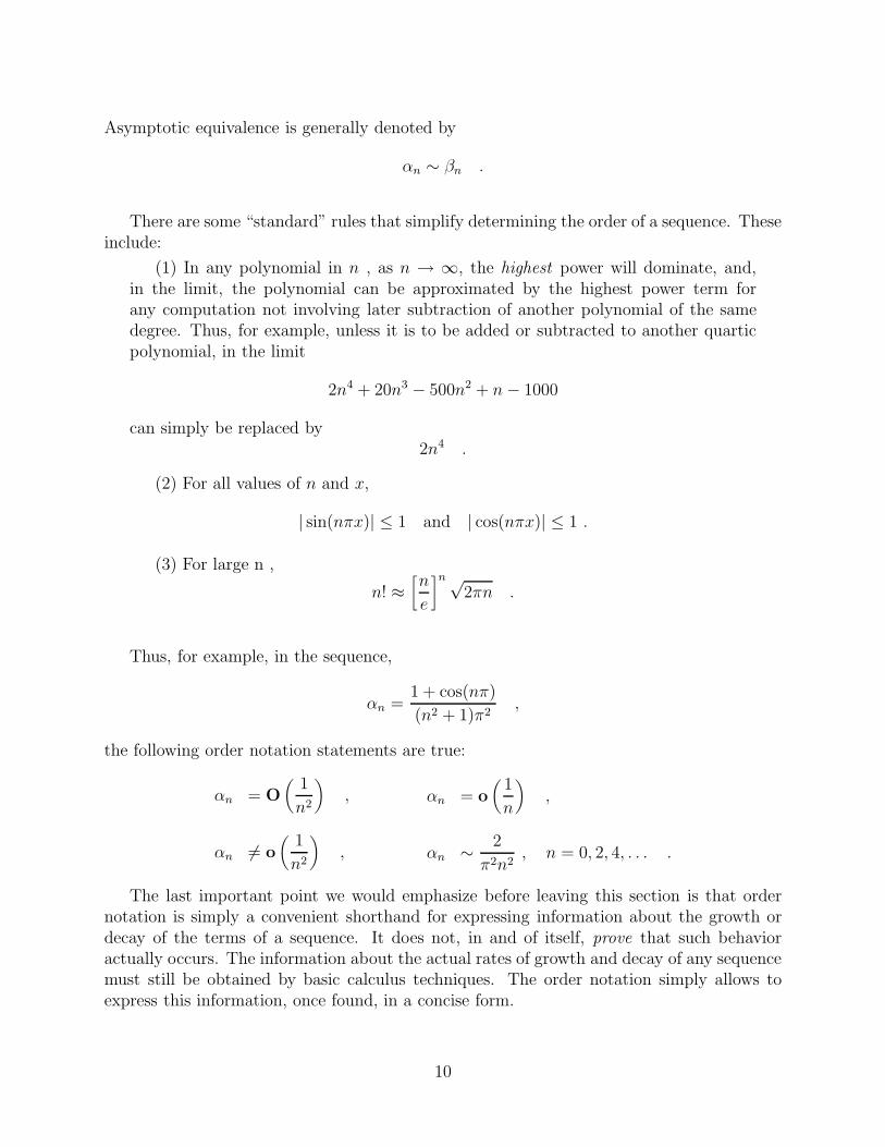
There are some “standard” rules that simplify determining the order of a sequence. Theseinclude:

(1) In any polynomial in n , as n → ∞, the highest power will dominate, and,in the limit, the polynomial can be approximated by the highest power term forany computation not involving later subtraction of another polynomial of the samedegree. Thus, for example, unless it is to be added or subtracted to another quarticpolynomial, in the limit

2n4 + 20n3 − 500n2 + n− 1000

can simply be replaced by2n4 .

(2) For all values of n and x,

| sin(nπx)| ≤ 1 and | cos(nπx)| ≤ 1 .

(3) For large n ,

n! ≈[n

e

]n√2πn .

Thus, for example, in the sequence,

αn =1 + cos(nπ)

(n2 + 1)π2,

the following order notation statements are true:

αn = O(

1

n2

),

αn = o(

1

n2

),

αn = o(

1

n

),

αn ∼ 2

π2n2, n = 0, 2, 4, . . . .

The last important point we would emphasize before leaving this section is that ordernotation is simply a convenient shorthand for expressing information about the growth ordecay of the terms of a sequence. It does not, in and of itself, prove that such behavioractually occurs. The information about the actual rates of growth and decay of any sequencemust still be obtained by basic calculus techniques. The order notation simply allows toexpress this information, once found, in a concise form.

10

1.5 Infinite Series

Again, we shall assume some prior familiarity with this topic on the part of the reader, andcover only some high points. By definition, an infinite series is formed by adding all theterms of a sequence. Note that in general, this theoretically requires adding together aninfinite number of terms. For example, if

an =(

2

3

)n

, n = 0, 1, 2, . . . ,

then the infinite series formed from an is

∞∑n=0

an = a0 + a1 + a2 + a3 + · · ·

=∞∑

n=0

(2

3

)n

= 1 +2

3+

4

9+

8

27+ · · ·

In the vernacular of FORTRAN, an infinite series is thus equivalent to a DO loop whoseupper limit is unbounded. Clearly, evaluation of an infinite series by direct addition, i.e. by“brute force,” is impractical, even physically impossible. This is the heart of Zeno’s paradox.As posed by the ancient Greeks, the paradox hinges on adding together an infinite numberof time intervals, each half of the previous one. The logical flaw in the Greeks’ analysis wasthe implicit assumption that the sum of an infinite number of non-zero terms was necessarilyinfinite. Correctly understanding this paradox requires the recognition that Zeno’s paradox,or for that matter any infinite series, involves the sum of an an infinite number of terms,and therefore the only valid method of analysis is in terms of limits.

The mathematical analysis of infinite series starts with the recognition that every infiniteseries in fact involves two sequences:

(1) The sequence of terms - an,

and

(2) The sequence of partial sums -

SN = a0 + a1 + · · ·+ aN

=N∑

n=0

an

If the sequence of partial sums itself then has a limit, i.e. if

limN→∞

SN = S

11

exists, then we can meaningfully talk of adding together the infinite number of terms in theseries and yet getting a finite answer. In such a case, we shall say the infinite series converges.(If the limit doesn’t exist, then we say the series diverges.) Fundamental to this definitionis the understanding that while ultimately convergence or divergence of the series dependson the terms (an), the primary quantity analyzed in deciding whether a series convergesor diverges is the sequence of partial sums (SN). Furthermore, and this frequently causesconfusion when students first encounter infinite series, since two sequences are involved, thereis always the possibility that one will converge and the other not. To be more precise, whilethe infinite series (sequence of partial sums) cannot converge if the sequence of terms doesnot, convergence of the sequence of terms of a series to a limit (even to a limit of zero) doesnot guarantee the infinite series will converge. Many examples exist where the sequence ofterms converges, but the series does not. One such series is given by:

an ≡ 1 , n = 0, 1, 2, . . .

SN =N∑

n=0

1 = 1 + 1 + · · ·+ 1 = N + 1 .

The above simple example illustrates another fundamental point about infinite series –determining the convergence or divergence of a series directly from the definition requiresfirst having (or finding) a formula for the partial sums. There are a few, but only a few,classic non-trivial cases in which this is possible. The most well-known example of these isthe geometric series:

SN =N∑

n=0

rn = 1 + r + r2 + · · ·+ rN

=1− rN+1

1− r , r = 1 ,

where r is any real number. With this formula, one can then show quite easily that

∞∑n=0

rn =

⎧⎪⎪⎨⎪⎪⎩

11−r,

|r| < 1

diverges otherwise

Coincidentally, this formula also resolves Zeno’s paradox. As we observed before, each time

interval in the paradox is exactly half of the previous interval. Therefore, assuming the firstinterval, i.e. the time from when the “race” starts until the runner reaches the tortoise’sinitial position, is one unit of time, the sequence of times is given by:

tn =(

1

2

)n

.

Hence, the time until the runner catches up with the tortoise is:∞∑

n=0

(12

)n=

1

1− 12

= 2 ,

which is exactly what common sense tells us it should be.

12

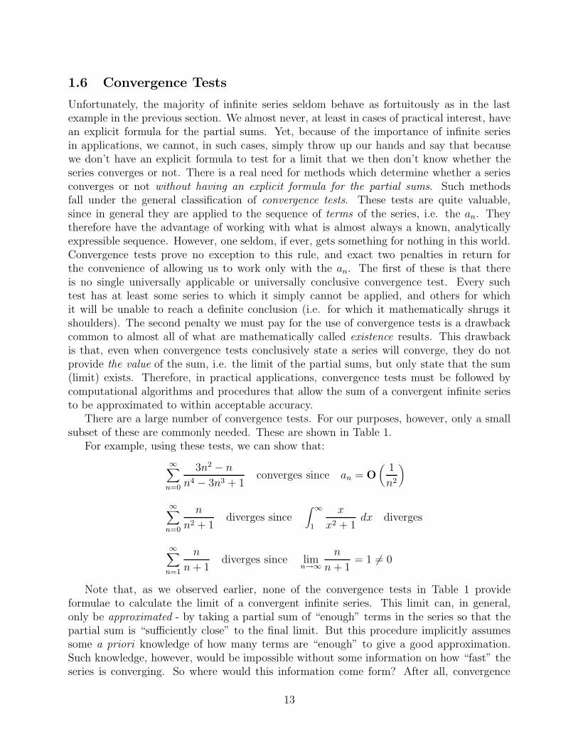
1.6 Convergence Tests

Unfortunately, the majority of infinite series seldom behave as fortuitously as in the lastexample in the previous section. We almost never, at least in cases of practical interest, havean explicit formula for the partial sums. Yet, because of the importance of infinite seriesin applications, we cannot, in such cases, simply throw up our hands and say that becausewe don’t have an explicit formula to test for a limit that we then don’t know whether theseries converges or not. There is a real need for methods which determine whether a seriesconverges or not without having an explicit formula for the partial sums. Such methodsfall under the general classification of convergence tests. These tests are quite valuable,since in general they are applied to the sequence of terms of the series, i.e. the an. Theytherefore have the advantage of working with what is almost always a known, analyticallyexpressible sequence. However, one seldom, if ever, gets something for nothing in this world.Convergence tests prove no exception to this rule, and exact two penalties in return forthe convenience of allowing us to work only with the an. The first of these is that thereis no single universally applicable or universally conclusive convergence test. Every suchtest has at least some series to which it simply cannot be applied, and others for whichit will be unable to reach a definite conclusion (i.e. for which it mathematically shrugs itshoulders). The second penalty we must pay for the use of convergence tests is a drawbackcommon to almost all of what are mathematically called existence results. This drawbackis that, even when convergence tests conclusively state a series will converge, they do notprovide the value of the sum, i.e. the limit of the partial sums, but only state that the sum(limit) exists. Therefore, in practical applications, convergence tests must be followed bycomputational algorithms and procedures that allow the sum of a convergent infinite seriesto be approximated to within acceptable accuracy.

There are a large number of convergence tests. For our purposes, however, only a smallsubset of these are commonly needed. These are shown in Table 1.

For example, using these tests, we can show that:

∞∑n=0

3n2 − nn4 − 3n3 + 1

converges since an = O(

1

n2

)

∞∑n=0

n

n2 + 1diverges since

∫ ∞

1

x

x2 + 1dx diverges

∞∑n=1

n

n+ 1diverges since lim

n→∞n

n+ 1= 1 = 0

Note that, as we observed earlier, none of the convergence tests in Table 1 provideformulae to calculate the limit of a convergent infinite series. This limit can, in general,only be approximated - by taking a partial sum of “enough” terms in the series so that thepartial sum is “sufficiently close” to the final limit. But this procedure implicitly assumessome a priori knowledge of how many terms are “enough” to give a good approximation.Such knowledge, however, would be impossible without some information on how “fast” theseries is converging. So where would this information come form? After all, convergence

13

Convergence Tests

1. If limn→∞an = 0, then

∑an diverges.

(This test is inconclusive if limn→∞ an = 0.)

2. The Absolute Convergence Test -If∑ |an| converges, then

∑an converges.

(This test is inconclusive if∑ |an| diverges.)

3. The Comparison Test -

Ifan

bn→ A and A = 0,±∞ , then

∑an and

∑bn either both converge or

both diverge.

4. The Alternating Series Test -If anan+1 < 0 (i.e. if the terms of the series alternate algebraic signs), if |an+1| ≤|an| and if lim

n→∞ an = 0 , then∑an converges.

5. The Integral Test -If an > 0 , and an = f(n) for a function f(x) which is positive and monotonically

decreasing, then∑an and

∞∫1f(x) either both converge or both diverge.

6. The p-Test -∞∑

n=1

1

npconverges if p > 1 ,diverges if p ≤ 1 .

7. The order np-Test -

If an = O(

1np

), p > 1, then

∞∑n=1

an converges.

8. The Geometric Series Test -∞∑n=0

rn converges if |r| < 1 .diverges if |r| ≥ 1 .

14

tests generally only provide the information that a given series converges. This only impliesthat the sequence of partial sums eventually approaches a limit - convergence tests provideno information about how fast the limit is being approached. For example, consider the twoseries: ∞∑

n=0

1

n!= e = 2.7183, and

∞∑n=1

1

n2=π2

6= 1.6449 ,

both of which converge according to one or more of the convergence tests, and the followingtable of their partial sums:

NN∑

n=0

1

n!

N∑n=1

1

n2

3 2.6667 1.36115 2.7167 1.4636

10 2.7183 1.5498100 2.7183 1.6350

Clearly, after ten times as many terms, the partial sum of one hundred terms of the secondseries does not provide as good an approximation to the value of that series than does aten-term partial sum of the first.

As alluded to above, determination of the rate of convergence of an infinite series is of farmore than just academic interest when we try to approximate the value of a convergent infi-nite series by computing a partial sum. Without some realistic way of determining how manyterms must be computed in order to obtain a “good” approximation, such a computationwould amount to little more than a mathematical shot in the dark. At best, we would takefar more terms than really necessary - getting an accurate result, although paying far toomuch in computational cost for it. At worst, however, we might stop our sum prematurely- and end up with a terribly inaccurate approximation. Fortunately, in the next section weshall see that if we have some idea of the order of the terms in a series, then we can in factestimate fairly well a priori how accurately a given partial sum will approximate the finalseries sum.

1.7 Error Estimates

Given that in general the only reasonable way to approximate the (unknown) sum of aninfinite series is by a partial sum, the natural measure for the accuracy of that approximationwould be the difference between the approximation and the actual sum. This measure is“natural” in that since the series converges, we know that

SN =N∑

n=0

an → S ,

15

where S is the sum of the series. Therefore, for “large” N , SN should be “close to” S, andso the error in approximating S by SN is simply:

EN = S − SN =∞∑

n=0

an −N∑

n=0

an

=∞∑

n=N+1

an .

On the face of it, this may not seem terribly illuminating, since in general only SN canbe known, and EN is just another (unknown) convergent series. However, as we shall see,in many cases, EN can be estimated , at least to its order of magnitude, and an order ofmagnitude estimate to EN is all that is needed to determine how many digits in SN aresignificant. Of course, obtaining such an estimate may not be trivial, since EN depends onboth an and N . But, for a reasonably large class of series, obtaining such error estimates isalso really not all that difficult.

Consider the infinite series ∞∑n=1

1

np, p > 1 .

Following our definition above, the error in approximating this series by any partial sum ofits terms is thus given by

EN =∞∑

n=N+1

1

np=

1

(N + 1)p+

1

(N + 2)p+

1

(N + 3)p+ · · · .

But now look at Figure 8. Note that since each rectangle in that figure has a base of lengthone, then the areas of those rectangles are, respectively,

1

(N + 1)p,

1

(N + 2)p,

1

(N + 3)p, . . . ,

and therefore the total shaded area under the blocks in Figure 8 is precisely equal to theerror, EN .

However, clearly the shaded (rectangular) area in Figure 8 is also strictly smaller than thearea under the curve in that figure. The importance of this observation is while we cannotcompute the sum of the error series exactly, we can compute the slightly larger integral.Thus we have ∞∑

n=N+1

1

np≤∫ ∞

N

dx

xp=

1

(p− 1)Np−1,

or, for this series

EN ≤ 1

(p− 1)Np−1.

The accuracy of this upper bound to EN can be checked for the case p = 2 , whose partialsums were computed in an earlier example, since in that case we know the exact value of theinfinite series, i.e.

∞∑n=1

1

n2=π2

6.

16

N N+1 N+2 N+3

1/xp

1/(N+1)p 1/(N+2)p1/(N+3)p

Figure 8: Estimating the Error of a Partial Sum

The results of computing the actual error and comparing it to the upper bound given by theintegral are shown in the following table:

N EN1

(p− 1)Np−1

3 0.28382 0.333335 0.18132 0.20000

10 0.09517 0.10000100 0.00995 0.01000

As this table demonstrates, the integral error bound in fact gives an excellent order ofmagnitude estimate to the error for N > 5 .

This last result, which was obtained for the very specific series an = 1np can be fairly

straightforwardly extended to any series whose terms are of O(

1np

)for p > 1 . This

happens because when

an = O(

1

np

),

then, for some constant C ,

|an| ≤ C

np.

But then, because the absolute value of a sum is less than or equal to the sum of the absolute

17

values of the terms in that sum, we have

|EN | =∣∣∣∣∣∣

∞∑n=N+1

an

∣∣∣∣∣∣ ≤∞∑

n=N+1

|an|

≤∞∑

n=N+1

C

np

≤∫ ∞

N

C

xpdx =

C

(p− 1)Np−1,

or

|EN | ≤ C

(p− 1)Np−1.

This last result can be restated as

if an = O(

1

np

), then EN = O

(1

np−1

).

Therefore, in such a series, doubling the number of terms used in a partial sum approxi-

mation reduces the error by a factor of1

2p−1. While this result does not generally provide

as tight bounds as in the case when the coefficients are exactly1

np, it nevertheless works

acceptably well in almost all cases.

1.8 Sequences of Functions

In our discussion of sequences and series thus far, we have implicitly been using a morerestrictive definition of a sequence than was necessary. Specifically we defined a sequenceto be a function defined on the integers, and considered a function to be any unique in-put/output black box. But in all our examples these were all only real-valued functions.There are, however, other sequences than just real-valued ones. For example, there are se-quences of functions - i.e. unique input/output black boxes, for which the only valid inputsare integers, but for which the outputs are not numbers, but other functions. For example

fn(x) = xn , n ≥ 0

(with the implicit understanding that x0 ≡ 1 ) defines a sequence of functions (graphs), thefirst few members of which are displayed in Figure 9.

Convergence of sequences of functions can be defined in a reasonably similar manner toconvergence of sequences of constants, since at a fixed x, the sequence of function valuesis in fact just a sequence of constants. Convergence of sequences of functions is differenthowever in that these values now depend not only on the functions in the sequence itself,but on the value of x as well. Thus,

fn(x)→ f(x)

18

f0(x)

f1(x)

f2(x)

f3(x)

f4(x)

f5(x)

−1 1

Figure 9: A Sequence of Functions

is, in some sense, an incomplete statement, until the values of x at which it holds true arealso specified. For example,

xn → 0

but only for −1 < x < 1 . Thus, to completely specify the behavior of this sequence, wewould have to state

xn → 0 , −1 < x < 1 ,

while,xn → 1 , x = 1 ,

and the sequence does not converge if either x ≤ −1 or x > 1 . Such behavior iscommonly referred to as pointwise convergence and divergence.

We would finally note that convergence of sequences of functions has a strong graphicalinterpretation, just as convergence of a sequence of constants could be viewed in terms oftables where the values do not change after some point. With sequences of functions, thepicture is one of a sequence of curves (graphs), which, eventually, begin to lie on top of eachother, until they finally become indistinguishable from the limit curve.

Infinite series of functions, e.g.∞∑

n=0

fn(x)

can also be defined similarly to infinite series of constants, since again, at any fixed x, aninfinite series of functions reduces to just a series of constants. Again, however, as with thesequence of functions, we must explicitly recognized that the resulting sequence of partialsums

SN(x) =N∑

n=0

fn(x)

19

depends on both N and x. Therefore, whether a given infinite series of functions convergesor diverges is generally affected by the choice of x. For example, for the sequence of functionsdefined above, the infinite series

∞∑n=0

xn

converges for all −1 < x < 1 (by the geometric series test) and therefore

∞∑n=0

xn =1

1− x , −1 < x < 1 .

(Note that this infinite series does not converge for x = 1 , even though the sequence ofterms (functions) does!)

Furthermore, even where a series of functions converges, the rate at which it converges,and hence the number of terms necessary for a good approximation, generally depends onthe value of x at which it is being evaluated. For example, we have an explicit formula forthe partial sum of the geometric series,

SN(x) =1− x(N+1)

1− x ,

and therefore it is fairly easily shown that

EN(x) =x(N+1)

1− x .

Clearly in this latter formula, EN(x) does depend on both N and x. The degree of thisdependence, however is perhaps more strikingly demonstrated by the following table, whichdisplays the error in approximating the sum of the above series for selected values of x andN .

x E5(x) E10(x)0.10 1.1× 10−6 1.1× 10−11

0.25 0.00033 3.1× 10−7

0.50 0.03125 0.000980.75 0.71191 0.168940.95 14.70183 11.37600

As with sequences of functions, this kind of convergence for infinite series of functions -where the convergence properties may vary with the value of x - is commonly referred to aspointwise convergence. While better than no convergence at all, pointwise convergence is notparticularly desirable, especially from a computational viewpoint, since any program usedto compute partial sums in such a case would have to be able to adjust the upper limit ofthe sum depending on the value of x. If for no other reason than programming convenience,we would far prefer that, given some desired accuracy criterion, there were a single number

20

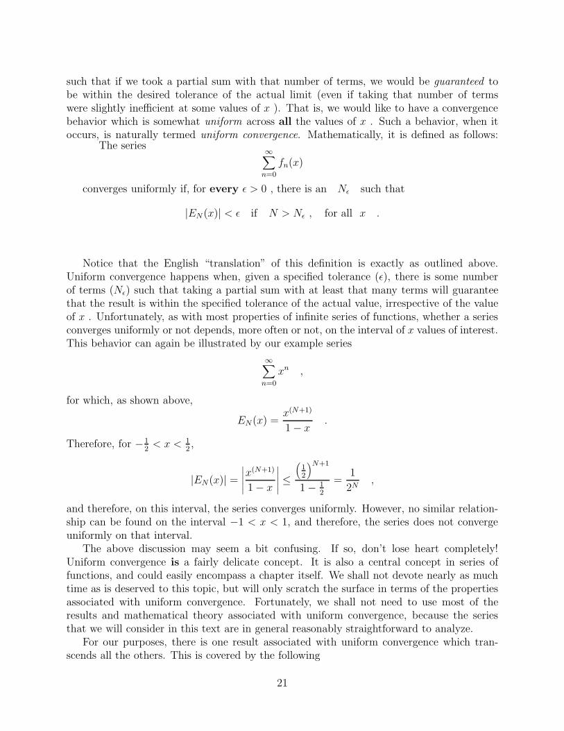
such that if we took a partial sum with that number of terms, we would be guaranteed tobe within the desired tolerance of the actual limit (even if taking that number of termswere slightly inefficient at some values of x ). That is, we would like to have a convergencebehavior which is somewhat uniform across all the values of x . Such a behavior, when itoccurs, is naturally termed uniform convergence. Mathematically, it is defined as follows:

The series ∞∑n=0

fn(x)

converges uniformly if, for every ε > 0 , there is an Nε such that

|EN (x)| < ε if N > Nε , for all x .

Notice that the English “translation” of this definition is exactly as outlined above.Uniform convergence happens when, given a specified tolerance (ε), there is some numberof terms (Nε) such that taking a partial sum with at least that many terms will guaranteethat the result is within the specified tolerance of the actual value, irrespective of the valueof x . Unfortunately, as with most properties of infinite series of functions, whether a seriesconverges uniformly or not depends, more often or not, on the interval of x values of interest.This behavior can again be illustrated by our example series

∞∑n=0

xn ,

for which, as shown above,

EN(x) =x(N+1)

1− x .

Therefore, for −12< x < 1

2,

|EN(x)| =∣∣∣∣∣x

(N+1)

1− x

∣∣∣∣∣ ≤(

12

)N+1

1− 12

=1

2N,

and therefore, on this interval, the series converges uniformly. However, no similar relation-ship can be found on the interval −1 < x < 1, and therefore, the series does not convergeuniformly on that interval.

The above discussion may seem a bit confusing. If so, don’t lose heart completely!Uniform convergence is a fairly delicate concept. It is also a central concept in series offunctions, and could easily encompass a chapter itself. We shall not devote nearly as muchtime as is deserved to this topic, but will only scratch the surface in terms of the propertiesassociated with uniform convergence. Fortunately, we shall not need to use most of theresults and mathematical theory associated with uniform convergence, because the seriesthat we will consider in this text are in general reasonably straightforward to analyze.

For our purposes, there is one result associated with uniform convergence which tran-scends all the others. This is covered by the following

21

Theorem If the series of functions∞∑

n=0fn(x) converges uniformly to a limit function

f(x) , and if each of the fn(x) is continuous, then f(x) is also continuous.

Note that this theorem does not tell whether any particular given series converges uniformlyor not, only what one may conclude after they have determined that series does convergeuniformly. Thus, for example, this theorem allows us to conclude that the sequence offunctions fn(x) = xn will converge to a continuous function for −1/2 < x < 1/2, but onlyafter we have determined, as we did above, that the sequence converged uniformly on thisinterval. The actual determination of whether any particular series converges uniformly, andwhere, is generally as difficult, or even more so, than determination of convergence of a seriesof constants. Fortunately however, for our purposes, there is one extremely easy-to-applytest for uniform convergence that will apply to most of the series we must deal with. Thistest - the so-called Weierstrass M-test - is really just another comparison test.

Theorem Given the sequence of functions fn(x), if there is a sequence of constants,Mn, such that on some interval a ≤ x ≤ b,

|fn(x)| ≤Mn and∞∑

n=0

Mn converges,

then∞∑

n=0

fn(x)

converges uniformly on that same interval

(Note that probably the only reason to call this the M-test is that Karl Theodore WilhelmWeierstrass2 called his sequence Mn instead of an. Had he done the latter, we would probablyall call this the Weierstrass a-test today! Furthermore, note that, the Weierstrass test suffersthe same limitations as do all convergence tests - there will be series to which it does notapply, and even when it shows that a series does converge uniformly, it does not provide anyinformation on what the limit of that series is.)

We can apply this theorem immediately to a problem very representative of the type ofinfinite series we shall deal with for the rest of this text -

∞∑n=1

1

n2cos(nx) = cos(x) +

1

4cos(2x) +

1

9cos(3x) + · · · .

For this series, the functions which form the sequence of terms satisfy the conditions of theWierstauss M-test,

|fn(x)| =∣∣∣∣ 1

n2cos(nx)

∣∣∣∣ ≤ 1

n2, for all x .

Therefore, since∞∑

n=1

1

n2converges ,

2see http://www-gap.dcs.st-and.ac.uk/∼history/Mathematicians/Weierstrass.html

22

we conclude that ∞∑n=1

1

n2cos(nx)

converges uniformly for all x, and therefore the infinite series represents a continuous func-tion.

23

PROBLEMS1. For each of the following sequences, determine if the sequence converges or diverges. Ifthe sequence converges, determine the limit

a. an =2n+1

3n+2b. an =

(n+ 1)2

5n2 + 2n+ 1c. an =

sin(n)

n+ 1

d. an = cos(n) e. an =2(n+ 1)2 + e−n

3n2 + 5n+ 10f. an =

n cos(nπ2

)

n + 1

g. an =cos(nπ)

n2 + 1h. an =

en

n!i. an =

n sin(nπ)

n+ 1

2. Determine the order (“big Oh”) of the following sequences

a. an =n3 + 2n2 + 1000

n7 + 600N6 + nb. an =

cos(nπ)

n2 + 1

c. an =[

n

n2 − 1− n

n2 + 1

]sin((n+

1

2)π)

d. an10n3e−n + n2

(2n+ 1)2cos(n2π)

3. Consider the infinite series ∞∑n=0

(n+ 1)22n

(2n)!

a. Compute, explicitely, the partial sums S3 and S6

b. Write the equivalent series obtained by replacing n by k−2, i.e. by shifting the index.

4. Determine whether each of the following infinite series diverges or converges:

a.∞∑

n=0

e−n b.∞∑

n=0

n2 + 1

(n+ 1)3c.

∞∑n=0

n2 cos(nπ)

(n3 + 1)2

d.∞∑

n=0

n

n+ 3e.

∞∑n=0

en

n!cos(nπ) f.

∞∑n=2

1

n ln(n)

5. Determine an (approximate) upper bound to the error when each of the following infiniteseries is approximated by a twenty-term partial sum (S20).

a.∞∑

n=0

2n+ 1

3n4 + n+ 1b.

∞∑n=1

1

n5c.

∞∑n=1

(2n + 1)2

n4

6. Consider the series: ∞∑n=0

xn

a. plot the partial sums S1(x), S5(x), S10(x), and S20(x) for −2 < x < 2.

b. What can you conclude about the convergence of the partial sums in this interval?

c. What, if anything, different can you conclude about the convergence of these partial

sums in the interval −1

2< x <

1

2.

24

2 Fourier Series

2.1 Introduction

In the last chapter we reviewed and discussed the concept of infinite series of functions.Such series, the first example of which most students encounter are the Taylor series, arefrequently used to approximate “complicated” functions in terms of “simpler” ones. Forexample, the transcendental function ex is exactly computable only at x = 0. However, theTaylor series,

∞∑n=0

xn

n!

can compute, to any desired degree of accuracy, approximate values for this complicatedfunction in terms of simple powers of x. In this chapter, we introduce what is almostwithout question the most commonly used infinite series of functions after the Taylor series -the Fourier series.

By definition, a Fourier series is an infinite series of the form:

f(x) =a0

2+

∞∑n=1

{an cos

(nπx

L

)+ bn sin

(nπx

L

)}, (2.1.1)

where L is some positive number. (Note that this form is, unfortunately, not quite universal.Some texts write the leading coefficient in the Fourier series as just a0, rather than as (a0/2).Still other texts will use the quantity (T0/2) instead of L. As we shall also try to pointout at the appropriate time, while there is nothing wrong with either of these alternativeformulations, they simply lead to what we feel are slightly more involved formulas.)

Since the Fourier series is an infinite series, then based on our earlier discussion, severalquestions should immediately come to mind. Among these, we shall consider the following:

1. For what kind of functions, f(x), can we write a Fourier series?

2. What are the convergence properties of Fourier series? (Equivalently, under whatgeneral conditions will a Fourier series converge?)

3. How are the coefficients, an and bn, related to the function f(x) ?

Our first insight into the general class of functions for which one can write Fourier seriescomes from the observation that all of the terms in (2.1.1) above are periodic of period 2L,e.g.

cos

(nπ(x+ 2L)

L

)= cos

(nπx

L+ 2nπ

)= cos

(nπx

L

), etc .

Hence, clearly, the Fourier series itself must also be periodic of period 2L, i.e.

f(x+ 2L) = f(x) . (2.1.2)

25

A function whose general behavior described by (2.1.2) is shown in Figure 10). The key, ofcourse, to periodicity is the repetitive nature of such functions. Furthermore, this repetitionshould be clearly evident from inspection of the graph. Lastly, observe that once we knowthat a given function f(x) is periodic, the value of L is very easily related to the graph, sincethe interval between repetitions is 2L.

−2L −L L 2L 3L

Figure 10: A General Periodic Function

These last few comments also dovetail quite nicely with our earlier ones that infiniteseries may offer a way of decomposing complicated functions into simple ones. Along theselines, we shall show more fully as this course develops exactly how the Fourier series providesa mechanism by which complicated periodic functions can be broken down into sums of sinesand cosines - the simplest of periodic functions.

2.2 Derivation of the Fourier Series Coefficients

We next turn to the question of how the coefficients in the Fourier series are related to thefunction f(x). There is, unfortunately, no single technique that will produce formulas forthe coefficients in any infinite series. You may recall, for example, that for Taylor series,

g(x) =∞∑

n=0

an(x− x0)n ,

repeated differentiation, followed by evaluation at x = x0, leads to the conclusion that thecoefficients are defined by

an =1

n!

dng

dxn(x0)

(which immediately implies that Taylor series can only be written for functions with aninfinite number of derivatives). We now show that a totally different approach determinesthe Fourier series coefficients (and simultaneously provides important insights into the typeof functions for which Fourier series actually can be written.) Our starting point is witha number of integral formulas - the so-called Orthogonality Integrals. As we shall see moreclearly as our study develops, such integrals are pivotal to Fourier analysis. The preciseformulas for these orthogonality integrals are

26

∫ L

−Lcos

(nπx

L

)cos

(mπx

L

)dx =

{0 , m = nL ,m = n

∫ L

−Lsin

(nπx

L

)sin

(mπx

L

)dx =

{0 , m = nL ,m = n

∫ L

−Lsin

(nπx

L

)cos

(mπx

L

)dx = 0, all m, n ,

(2.2.3)

where m and n are any positive integers. There is, at least on the surface, nothing partic-ularly extraordinary about these integrals. They can easily be verified by standard calculustechniques. One simply uses standard trigonometric identities, such as

cos(a) cos(b) =cos(a+ b) + cos(a− b)

2

to reduce the integrand to a sum of elementary functions, then finds the antiderivative, andfinally evaluates that antiderivative at the end points, using the fact that

sin(kπ) = 0 , and cos(kπ) = cos(−kπ)

for any integer k.Given these orthogonality integrals, however, we can proceed to reduce (2.1.1) as follows.

Let m denote some fixed, but arbitrary positive integer. (This means that all we may assumeabout m is that it is positive and an integer. It need not necessarily be even; or odd; large orsmall; etc. We simply cannot assume that any steps are valid that require more informationthan the fact that m is a positive integer.) We shall then multiply both sides of (2.1.1) by

cos(

mπxL

), then, using the property that the integral of a sum is the sum of the respective

integrals, integrate the series formally, term by term, from −L to L. Performing all of thesesteps leads to the equation

∫ L

−Lf(x) cos

(mπx

L

)dx =

a0

2

∫ L

−Lcos

(mπx

L

)dx

+∞∑

n=1

{an

∫ L

−Lcos

(nπx

L

)cos

(mπx

L

)dx

+ bn

∫ L

−Lsin

(nπx

L

)cos

(mπx

L

)dx

}.

(2.2.4)

(Mathematically, we say this integration is formal because there is really some analyticuncertainty about the validity of interchanging the operations of integration and infinitesummation. In fact, in certain other infinite series (none of them Fourier series), interchang-ing these operations can in fact be shown to produce totally incorrect results. The readershould rest assured however that it can be rigorously proven that, for Fourier series, thisinterchange can be shown to be valid, although any proof of this claim is far beyond thescope of our discussion here).

27

Returning to (2.2.4), we can now use elementary integration techniques to show that,since m = 0, the first integral on the right hand side is identically zero. But now look atthe rest of this expression closely. Remember that the series notation implies that the termsinside the brackets must be evaluated for every positive integer n, then these values summed.But wait! If m is a positive integer then, by the orthogonality integrals (2.2.3), every termon the right side will be identically zero, except one. The single non-zero term will be thecosine integral that arises the one time inside the summation when the value of n equals m.Somewhat more graphically, this means the entire right-hand of the previous equation obeys

a0

2

∫ L

−Lcos

(mπx

L

)dx︸ ︷︷ ︸

=0

+∞∑

n=1

⎧⎪⎪⎪⎨⎪⎪⎪⎩an

∫ L

−Lcos

(nπx

L

)cos

(mπx

L

)dx︸ ︷︷ ︸

=0 , m�=n

+ bn

∫ L

−Lsin

(nπx

L

)cos

(mπx

L

)dx︸ ︷︷ ︸

=0 , all m,n

⎫⎪⎪⎪⎬⎪⎪⎪⎭ .

and therefore (2.2.4) simplifies to:

∫ L

−Lf(x) cos

(mπx

L

)dx = am

∫ L

−Lcos2

(mπx

L

)dx

or, solving for am and using the value of the orthogonality integral for cosines with m = n,

am =1

L

∫ L

−Lf(x) cos

(mπx

L

)dx , m > 0 .

But now, note that since m was designated as fixed, but arbitrary, this last equation is infact simply a formula for am. Therefore we can equally well now replace m by n on bothsides of this expression, and rewrite it as:

an =1

L

∫ L

−Lf(x) cos

(nπx

L

)dx . (2.2.5)

We can derive a similar formula for the bn,

bn =1

L

∫ L

−Lf(x) sin

(nπx

L

)dx , (2.2.6)

by multiplying both sides of (2.1.1) by a sine and integrating. Finally, a0 can be determined

by observing that the average values of both cos(

nπxL

)and sin

(nπxL

)are zero over any

whole number of cycles or periods. Thus their average value over the interval from −L to Lis zero. Hence the average value of every term under the summation sign is zero, and thusthe average value of the entire right-hand side of (2.1.1) is precisely

a0

2.

28

Since the average value of the left-hand side can be computed as

1

2L

∫ L

−Lf(x)dx ,

then clearly, after equating these two expressions and canceling the factors of two, we have

a0 =1

L

∫ L

−Lf(x)dx . (2.2.7)

(Equivalently, if one likes the brute force approach, they may simply integrate both sidesof (2.1.1) from −L to L, show the integrals under the summation sign are identically zero,and arrive at exactly the same result. While there would obviously be nothing wrong withthat approach, we generally prefer to use physical insight wherever possible.) You mightnote now that (2.2.7) is precisely what we would obtain by letting n = 0 in (2.2.5), eventhough (2.2.5) was originally derived assuming n > 0. This is exactly why we adopted the(seemingly) rather awkward form for the leading coefficient in (2.1.1), since we now see thatby writing the constant term in the series as a0/2, we are able to use (2.2.5) to represent allthe an’s in the series, not just those for which n is positive. (Unfortunately, however, we willstill generally have to compute a0 separately, in order to avoid an antiderivative with a zerodenominator. However our representation still leaves one less formula to remember.)

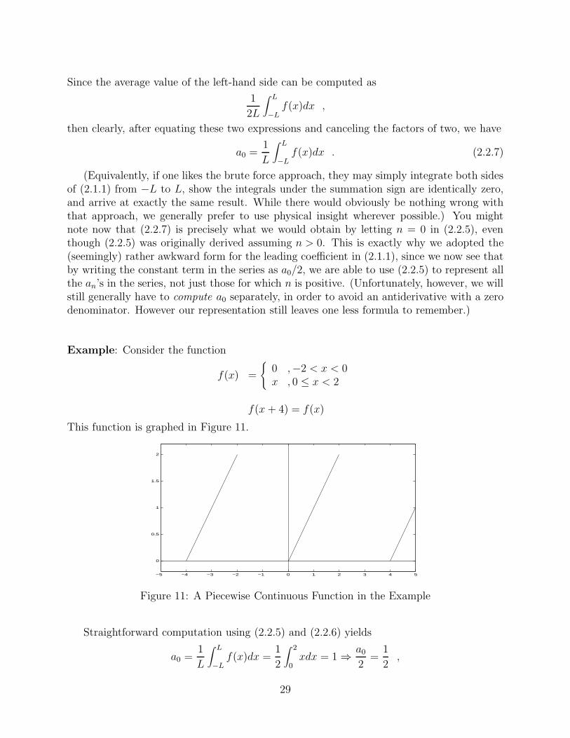
Example: Consider the function

f(x) =

{0 ,−2 < x < 0x , 0 ≤ x < 2

f(x+ 4) = f(x)

This function is graphed in Figure 11.

−5 −4 −3 −2 −1 0 1 2 3 4 5

0

0.5

1

1.5

2

Figure 11: A Piecewise Continuous Function in the Example

Straightforward computation using (2.2.5) and (2.2.6) yields

a0 =1

L

∫ L

−Lf(x)dx =

1

2

∫ 2

0xdx = 1⇒ a0

2=

1

2,

29

an =1

L

∫ L

−Lf(x) cos

(nπx

L

)dx =

1

2

∫ 2

0x cos

(nπx

2

)dx

=1

2

[2x

nπsin

(nπx

2

)+(

2

nπ

)2

cos(nπx

2

)] ∣∣∣∣∣2

0

=2

n2π2(cos(nπ)− 1) ,

and

bn =1

L

∫ L

−Lf(x) sin

(nπx

L

)dx =

1

2

∫ 2

0x sin

(nπx

2

)dx

=1

2

[− 2x

nπcos

(nπx

2

)+(

2

nπ

)2

sin(nπx

2

)] ∣∣∣∣∣2

0

= − 2

nπcos(nπ)) .

Thus, combining these, we have

f(x) =1

2+

∞∑n=1

{2

n2π2(cos(nπ)− 1) cos

(nπx

2

)− 2

nπcos(nπ) sin

(nπx

2

)}

=1

2− 4

π2cos

(πx

2

)+

2

πsin

(πx

2

)− 1

πsin(πx)

− 4

9π2cos

(3πx

2

)+

2

3πsin

(3πx

2

)+ · · ·

You should realize at this point that the above result may in fact be quite meaningless,for we have not yet proven that this series even converges! In fact, this is an appropriateplace to review exactly what the above infinite series notation represents, and what we meanby convergence.

By definition, when we write the Fourier series representation (2.1.1), we mean that, ifwe were to consider the sequence of partial sums given by:

SN(x) =a0

2+

N∑n=1

{an cos

(nπx

L

)+ bn sin

(nπx

L

)}, (2.2.8)

then,lim

N→∞SN (x) = f(x) .

But, as the notation clearly implies, these partial sums are functions, i.e. they have graphs.Thus, if a Fourier series converges, there should be some sequence of graphs, given by pre-cisely the graphs of these partial sums, that look “more and more like f(x)” the “larger” N

30

is. To demonstrate this in the example above, we have plotted, in Figure 12, several partialsums of the series we just derived. These graphs clearly seem, for larger values of N , to lookprogressively more like the original f(x), and therefore, in this example, the series founddoes appear to converge to f(x).

−2 −1 0 1 2−0.5

0

0.5

1

1.5

2

−2 −1 0 1 2−0.5

0

0.5

1

1.5

2

−2 −1 0 1 2−0.5

0

0.5

1

1.5

2

−2 −1 0 1 2−0.5

0

0.5

1

1.5

2

2.5

Figure 12: Convergence of the Partial Sums of a Fourier Series

Always having to generate such a set of graphs in order to confirm convergence, however,could clearly become quite cumbersome. Therefore, as part of our study, we will consider thegeneral convergence properties of the Fourier series, and classify those functions for whichFourier series can be guaranteed to converge before such graphs are even plotted.

We start by developing a bit more complete characterization of precisely the kind offunctions for which it “makes sense” to try to write a Fourier series, i.e. for which we shouldeven try to compute an and bn as given by (2.2.5) and (2.2.6). Observe that computing an

and bn requires evaluating definite integrals. Therefore, since cos(

nπxL

)and sin

(nπxL

)are

continuous, it seems almost self-evident, from basic calculus considerations, that f(x) cannotbe “too far away” from being a continuous function. This initial impression is basicallycorrect, although the precise condition is slightly more involved and its proof far beyond thescope of our discussion here. Therefore, we simply state the most commonly used result onwhich functions will have convergent Fourier series:

Theorem: The function f(x) will have a convergent Fourier series, with coefficients an

31

and bn given by:

an =1

L

∫ L

−Lf(x) cos

(nπx

L

)dx , n ≥ 0

and

bn =1

L

∫ L

−Lf(x) sin

(nπx

L

)dx , n > 0 .

provided f(x) is periodic of period 2L, and both f(x) and f ′(x) are at least piecewisecontinuous on −L < x < L.

A piecewise continuous function is, of course, one composed of a finite number of continuoussegments (“pieces”) on any finite interval. To be more precise,Definition. A function f(x) is piecewise continuous in [a, b] if there exists a finite number ofpoints a = x1 < x2 < . . . < xn = b, such that f is continuous in each open interval (xj , xj+1)and the one sided limits f(xj+) and f(xj+1−) exist for all j ≤ n− 1.

The most common examples of such functions are those that are continuous except for“jump” discontinuities. The function we used in our last example is one of these, and satisfiesthe conditions of this theorem, since it is continuous everywhere except for jumps at x = ±2,and differentiable everywhere except at the jumps and at the sharp point at x = 0. (Func-tions for which f ′(x) is piecewise continuous are often called piecewise smooth.)

Our second consideration is the question of precisely how a Fourier series converges ata “jump” discontinuity. The proof of the answer, as with the proof of the above existencetheorem, is well beyond the scope of our discussion. But it can be shown that, at a “jump,”the Fourier series takes essentially the “path of least resistance” by converging to the averagevalue, i.e. at a jump

SN(x)→ f(x+) + f(x−)

2.

where f(x+) and f(x−) refer to the right- and left-hand limits, respectively (e.g. f(x+)means limε→0 f(x+ ε), where ε is positive.)

Thus far then, we have introduced the Fourier Series, shown how the Fourier coeffi-cients, an and bn can be computed, and for one example, displayed graphically the conver-gence of the resulting series.

32

PROBLEMS

1. Derive the formula for the Fourier sine coefficients, bn (eqn. (2.2.6)), using a methodsimilar to that used to derive eqn. (2.2.5).

2. For each of the following functions, find the Fourier coefficients, the Fourier series, andsketch the partial sums S2(x), S5(x), and S10(x):

a. f(x) =

{0 , −1 < x < 01 , 0 ≤ x < 1

f(x+ 2) = f(x)

b. f(x) =

{3 + x , −3 < x < 03− x , 0 ≤ x < 3

f(x+ 6) = f(x)

c. f(x) =

⎧⎪⎨⎪⎩

0 , −2 < x < 0x , 0 ≤ x < 1

2− x , 1 ≤ x < 2

f(x+ 4) = f(x)

d. f(x) = 1− cos(πx), −1 ≤ x ≤ 1

3. a. Show that the alternative Fourier Series representation

f(x) = a0 +∞∑

n=1

{an cos

(nπx

L

)+ bn sin

(nπx

L

)}

leads to the formulas

a0 =1

2L

∫ L

−Lf(x)dx ,

an =1

L

∫ L

−Lf(x) cos

(nπx

L

)dx , n > 0

bn =1

L

∫ L

−Lf(x) sin

(nπx

L

)dx , n > 0

where the formula for a0 is no longer the n = 0 special case of the formula for an.

33

b. Show that the alternative Fourier Series representation

f(t) =a0

2+

∞∑n=1

{an cos

(2nπt

T0

)+ bn sin

(2nπt

T0

)}

(note the independent variable here is t), where L has been replaced by T0/2, leads to

an =2

T0

∫ T0/2

−T0/2f(x) cos

(2nπt

T0

)dt , n ≥ 0

bn =2

T0

∫ T0/2

−T0/2f(x) sin

(2nπt

T0

)dt , n > 0 .

Note that here the formula for a0 is again the n = 0 special case of the formula for an.

4. In each of the following, find each point in −L < x < L where f(x) has a discontinuity.Find the left and right-hand limits of f(x) and f ′(x) at each point of discontinuity and atthe end points of the interval. Without computing the Fourier coefficients, indicate to whatvalues the series should converge at these points.

a. f(x) =

⎧⎪⎨⎪⎩x2 , 1 ≤ x ≤ 30 , −2 ≤ x < 12x , −3 ≤ x < −2

b. f(x) =

{3 , π/2 ≤ x ≤ π

2x− 2 , −π ≤ x < π/2

c. f(x) =

⎧⎪⎨⎪⎩

x2 , −2 ≤ x < 00 , 0 ≤ x < 1

4(x− 1) , 1 ≤ x ≤ 2

34

2.3 Odd and Even Functions

As we saw in the previous section, we can use the Fourier series to represent any appropriateperiodic function as a combination of the basic trigonometric functions of sine and cosine.Furthermore, once we have verified that a particular function satisfies the necessary con-ditions to have a Fourier series representation, determining the coefficients (i.e. an and bn)using (2.2.5) and (2.2.6) is a straightforward, although perhaps quite laborious exercise inintegration.

In this section, we show that we can sometimes significantly reduce the amount of com-putation necessary to construct a particular Fourier series representation by exploiting sym-metries in the function f(x). We start by observing that inspection of the graphs of sine andcosine (Figure 13) shows that both of these functions possess certain natural symmetries.Specifically, cosine is a perfect reflection (symmetric) with respect to the y-axis, and sine isan inverted (anti-symmetric) one. Thus, it is not unreasonable to expect a strong connec-tion between the symmetries (if any) in some periodic function, f(x), and the presence (orabsence) of sine or cosine terms in its Fourier series. We now show that this is in fact thecase.

−4 −2 0 2 4−1

−0.8

−0.6

−0.4

−0.2

0

0.2

0.4

0.6

0.8

1

−4 −2 0 2 4−1

−0.8

−0.6

−0.4

−0.2

0

0.2

0.4

0.6

0.8

1

Figure 13: Symmetries in Sine and Cosine

The symmetry and anti-symmetry described above are identical to that of the various powersof x , i.e. xn, depending on whether the exponent (n) is even or odd. Therefore, symmetryand anti-symmetry, when they exist, are more commonly referred to, respectively, as evenor odd. To be precise,

DEFINITION:A function f(x) is even if f(x) = f(−x) for all x.A function f(x) is odd if f(x) = −f(−x) for all x.

We would hasten to caution that there are functions which have no such symmetries, i.e.which are neither even nor odd. (The first example in the last section is one such function.)Furthermore, no non-trivial function can be both even and odd. But when one is dealingwith either an even or odd function, there are several rules that can simplify calculations.Among the most useful of these rules are the following:

1. The product of two even functions is even,

35

2. The product of two odd functions is even,

3. The product of an even and odd function is odd,

4. The derivative of an even function is odd,

5. The derivative of an odd function is even,

6. If g(x) is even, then ∫ L

−Lg(x)dx = 2

∫ L

0g(x)dx

7. If g(x) is odd, then ∫ L

−Lg(x)dx = 0 .

All of the above statements are straightforward to prove, and generally follow immediatelyfrom the definitions of even and odd. The statements about the integrals reflect the facts,evident from Figure 14, that an even function sweeps out equal areas on both sides of they axis, and an odd function does almost the same thing, except that with an odd functionthese areas differ in algebraic sign, and so cancel.

Figure 14: Integrals of Even and Odd Functions

Now, applying these properties to Fourier series leads to the observation:

If f(x) is even, then

⎧⎨⎩ f(x) cos

(nπxL

)is even, and

f(x) sin(

nπxL

)is odd

However, by the integral properties above, it follows immediately from this last statementthat if f(x) is even and has a Fourier series, then by (2.2.5) and (2.2.6) in the previoussection,

an =2

L

∫ L

0f(x) cos

(nπx

L

)dx

36

andbn = 0 .

Thus for an even function

f(x) =a0

2+

∞∑n=1

an cos(nπx

L

)

Similarly, we can show that if f(x) is odd, then

f(x) =∞∑

n=1

bn sin(nπx

L

)

where

bn =2

L

∫ L

0f(x) sin

(nπx

L

)dx .

We must emphasize that these results are not really different from, and do not produceany information not already contained in the basic Fourier series coefficient formulas ((2.2.5)and (2.2.6)). They simply are a means to reduce the computational burden in selected casesby indicating, ahead of time, which coefficients should be identically zero. One would obtainidentical values the “long way,” i.e. using (2.2.5) and (2.2.6) directly, but only after muchmore effort and an increased chance of algebraic error.

Thus, for example, with the odd function shown below

−6 −4 −2 0 2 4 6−4

−3

−2

−1

0

1

2

3

4

Figure 15: f(x) = x , − 3 < x < 3

we can immediately claim that

f(x) =∞∑

n=1

bn sin(nπx

3

),

where

bn =2

3

∫ 3

0x sin

(nπx

3

)dx = − 6

nπcos(nπ) .

and not have to bother computing the an, since we know they must be identically zero.The above results on odd and even functions can also be used to simplify computation

in a number of further cases where the addition or subtraction of a constant will convert

37

an otherwise unsymmetric function to an odd function. (Note addition or subtraction of aconstant will not alter the evenness of a function.) For example, the function

f(x) = 4 + x , − 3 < x < 3,f(x+ 6) = f(x) ,

is neither even nor odd, but [f(x)− 4] is clearly odd. Hence we could write,

f(x) = 4 +∞∑

n=1

bn sin(nπx

3

),

where the bn are as computed above.

38

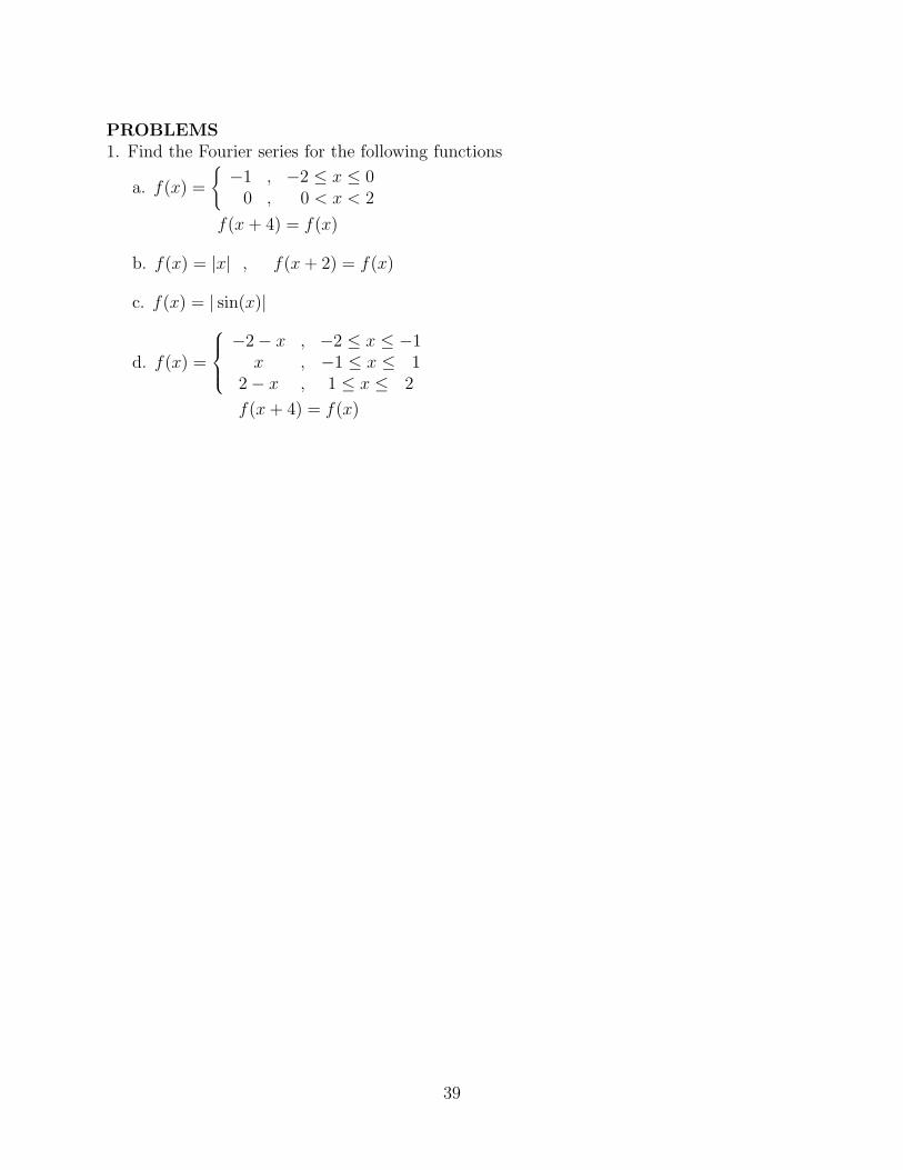
PROBLEMS1. Find the Fourier series for the following functions

a. f(x) =

{ −1 , −2 ≤ x ≤ 00 , 0 < x < 2

f(x+ 4) = f(x)

b. f(x) = |x| , f(x+ 2) = f(x)

c. f(x) = | sin(x)|

d. f(x) =

⎧⎪⎨⎪⎩−2− x , −2 ≤ x ≤ −1x , −1 ≤ x ≤ 1

2− x , 1 ≤ x ≤ 2

f(x+ 4) = f(x)

39

2.4 Convergence Properties of Fourier Series

In the previous sections, we have seen that a Fourier series can be written, at least formally,for the periodic (of period 2L) function f(x), as

f(x) =a0

2+

∞∑n=1

{an cos

(nπx

L

)+ bn sin

(nπx

L

)}

where

an =1

L

∫ L

−Lf(x) cos

(nπx

L

)dx , n = 0, 1, 2, . . .

bn =1

L

∫ L

−Lf(x) sin

(nπx

L

)dx , n = 1, 2, . . .

Obviously, given a particular f(x), there would be little point in bothering to computethese integrals without some assurance the resulting series would converge, and so we citedearlier some theorems involving an extremely straightforward test (i.e. if f(x) is at leastpiecewise smooth) that, if satisfied, would guarantee that the series constructed using theabove coefficients will in fact converge. However, as we shall see later, another, equallyimportant consideration frequently arises in the study of Fourier series. There are oftenoccasions where one must deal with a Fourier series, by itself, with no explicit identificationof the function f(x) which it represents. In such cases, one would like to be able to infer,from examining the series itself (i.e. the coefficients), not only whether it converges, but also,if it does, what general characteristics does the function it represents possess? Therefore,motivated by both of these concerns, we shall now investigate in greater detail the exactmechanisms which drive the convergence of Fourier series. During this study, our primarygoal will be to more fully understand the interrelationships between the properties of thefunction f(x) and the general behavior of the coefficients, an and bn.

We start by recalling that the primary vehicle for describing the quantitative convergenceproperties of any infinite series is the error remaining after approximating the series by apartial sum. In the case of the Fourier series, this error is given by the formula:

EN(x) = f(x)− SN (x) =∞∑

n=N+1

{an cos

(nπx

L

)+ bn sin

(nπx

L

)}(2.4.9)

where SN(x) was given by equation (2.2.8). As we have already discussed at some lengthduring our consideration of general infinite series of functions, and as this formula alsoemphasizes, both this error and the associated rate of convergence of the series will, ingeneral, depend on the value of x at which we are evaluating the series. Furthermore, theFourier series will converge pointwise to f(x) if and only if

limN→∞

[EN(x)] = 0 at all values of x .

Lastly, a Fourier series will converge uniformly, and hence the limit function, f(x), be con-tinuous, if and only if

|EN(x)| ≤ εN and limN→∞

[εN ] = 0 . (2.4.10)

40

But now look carefully at (2.4.9). Specifically, note that∣∣∣∣cos(nπx

L

)∣∣∣∣ ≤ 1 and∣∣∣∣sin

(nπx

L

)∣∣∣∣ ≤ 1

for all x. Therefore, if we take absolute values on both sides of (2.4.9), and use the fact thatthe absolute value of a sum is less than or equal to the sum of the absolute values, we have:

|EN(x)| ≤∞∑

n=N+1

{|an|+ |bn|} . (2.4.11)

There is, of course, no guarantee that the series on the right here will converge, but, if itdoes, then we have clearly satisfied the condition given by (2.4.10) and hence would have auniformly convergent series. We formally state these observations in:

THEOREM: The Fourier series for f(x) converges uniformly, and therefore f(x) is con-tinuous, if

∞∑n=1

{|an|+ |bn|} converges .

Observe that a major part of the value of this theorem is that it involves only a seriesof constants, whose convergence can therefore be easily tested by the usual tests, e.g.the integral test or the O (1/np) test. In fact, based on our earlier discussion on series ofconstants, we can immediately conclude the more practically useful:

COROLLARY: The Fourier series for f(x) will converge uniformly, and therefore f(x)will be continuous, if both an and bn are

O(

1

np

)for p > 1 .

(Before proceeding, we need to emphasize one point about the use of the term “continuous”in discussions of Fourier series. Remember that the Fourier series implicitly considers thefunction f(x) to be periodic. Thus, when f(x) is given explicitly in some interval, and justassumed to be continued periodically, as in:

f(x) =

{0 , − 2 < x < 0x , 0 ≤ x < 2

f(x+ 4) = f(x)(2.4.12)

it is continuous in the context used in the above only if f(x) is continuous not only onthe given interval, but also at the end points where it begins to periodically repeat itself.Thus the function given above is not continuous in the context of Fourier series theorems,even though it is continuous for −2 < x < 2, because it has a jump discontinuity at x = ±2.Several texts try to avoid this confusion, when discussing continuity, by speaking about theperiodic continuation of f(x), rather than just referring to f(x).)

41

The above discussion and theorem fairly well specify the conditions on the coefficientsunder which a Fourier series will converge to a continuous function. However, we can’t reallystop yet, since, as we saw when we computed the Fourier series for (2.4.12) in the firstsection, and as the theorem cited there indicates, formally constructed Fourier series canalso converge (at least in some cases) to discontinuous functions. (A discontinuous function,however, clearly can not have a uniformly convergent Fourier series. Moreover, based onthe preceding discussion, it appears virtually certain that when a Fourier series converges to

a discontinuous function, then either∞∑

n=1|an| or

∞∑n=1|bn| (or both) must diverge - a situation

seemingly destined to be the case if either the an or the bn “look like” 1/n. This seems tobe exactly what occurred in the Fourier series for (2.4.12).) But one or two examples ofdiscontinuous functions which have Fourier series do not a general theory make. Thus, weare still left with the unanswered question of whether all Fourier series in which at least oneof the coefficients is only O (1/n) converge? And, if so, what drives this convergence, sincethe series on the right in (2.4.11) can not converge in such a case?

In order to understand the answer to these last questions, we first need to introduce theconcept of the mean square measure. Specifically, for a given function f(x), the integral

1

2L

∫ L

−L[f(x)]2dx (2.4.13)

is called the mean square value of f(x) on the interval (−L,L). Physically you shouldrecognize that it can be interpreted as essentially a measure of the average energy representedby the function in this interval. If however, we now apply this integral to measure what isin effect the average energy contained in the error in a Fourier series approximation, andexpand the squared series, we have

1

2L

∫ L

−L[EN (x)]2 dx =

1

2L

∫ L

−L

⎡⎣ ∞∑

n=N+1

{an cos

(nπx

L

)+ bn sin

(nπx

L

)}⎤⎦2

dx

=1

2L

∫ L

−L

⎡⎣ ∞∑

n=N+1

{a2

n cos2(nπx

L

)+ b2n sin2

(nπx

L

)}

+∑∞∑m,n=N+1

m�=n

{aman cos

(nπx

L

)cos

(mπx

L

)

+ bmbn sin(nπx

L

)sin

(mπx

L

)}

+∑∞∑m,n=N+1

ambn cos(mπx

L

)sin

(nπx

L

)]dx

But now look what happens if we interchange the summations and integration (assumingagain that such interchanges are mathematically valid). All of the integrals involved become

42

orthogonality integrals (3), and more precisely, all of the terms in the double series areorthogonality integrals which integrate to zero! Thus, this last equation simply reduces to:

1

2L

∫ L

−L[EN (x)]2 dx =

1

2

∞∑n=N+1

{a2

n + b2n}

(2.4.14)

While this equation may not look especially significant, you should look at it carefully, forit actually embodies one of the basic properties of Fourier series! Because of the importanceof this relation to the understanding of these series, we shall investigate it in some detail,starting with the observation that (2.4.14) implies that

limN→∞

{1

2L

∫ L

−L[EN (x)]2 dx

}= 0 if

∞∑n=1

{a2

n + b2n}

converges.

Note the key difference between this last situation (i.e. convergence of the sequence ofsquares) and our earlier theorem on uniform convergence! Specifically, the series of squarescan converge even though

∞∑n=1

{|an|+ |bn|}

diverges! (This, again, will almost certainly arise when either an and bn, or both, are onlyO (1/n) - precisely the case we frequently encounter.) Clearly, now,

limN→∞

{1

2L

∫ L

−L[EN(x)]2 dx

}= 0 (2.4.15)

represents some type of convergence - but what kind? Is this simply one of the types we havealready discussed, in a different form, or is it fundamentally new? By our last comments, this“new” convergence can apparently occur even when the series does not converge uniformly,therefore it must be different from uniform convergence. Even more interestingly, this “new”convergence can occur even when the series does not converge pointwise to f(x), i.e. evenwhen EN (x) does not approach zero for all values of x. The reason for this perhaps surprisingstatement is that it is possible for

∫ L

−L[g(x)]2 dx = 0

even though g(x) ≡ 0, provided g(x) is discontinuous, bounded, and nonzero at only a finitenumber of points. (This is simply a generalization of the notion that the area under a pointis zero.) In other words, (2.4.15) may occur even though SN(x) does not converge to f(x)everywhere, but only almost everywhere, that is when

limN→∞

SN(x) = f(x)

except at a finite number of points. These points, of course, must have been points ofdiscontinuity in f(x) to begin with.

43

Since we have now shown this “new” convergence as defined by (2.4.15) does not coincidewith either uniform or pointwise convergence, it needs its own distinctive title. Perhaps notvery imaginatively, it is normally called convergence in the mean-square, or simply mean-square convergence. To be precise:

DEFINITION: The sequence of functions SN(x) will be said to converge to the func-tion f(x) in the mean-square sense, or almost everywhere, if

limN→∞

{1

2L

∫ L

−L[SN(x)− f(x)]2 dx

}= 0 . (2.4.16)

From our point of view, mean-square convergence is important because it not only describesa convergence that appears to be different from both uniform and pointwise convergence,but also a convergence which apparently governs the convergence of Fourier series for dis-continuous functions. We can incorporate most of the insights of this recent discussion intothe following:

THEOREM: The Fourier series for f(x) converges in the mean-square sense if

∞∑n=1

{a2

n + b2n}

converges.

Moreover, as with the theorem for uniform convergence, we can also immediately concludea more practically applicable

COROLLARY: The Fourier series for f(x) will converge in the mean-square sense ifboth an and bn are

O(

1

n

).

We must again emphasize most strongly that mean-square convergence does not nec-essarily imply that the SN(x) converge to f(x) at every point in (−L,L), although thiscertainly could be the case. mean-square convergence describes essentially a convergencein terms of energy rather than a pointwise convergence. Therefore, when we say a seriesconverges in the mean-square sense to f(x), we are in effect saying that f(x) and the limit ofthe series differ, at most, in a function which contains no energy and is therefore physicallyuninteresting.

To recap our development to this point, we have thus far established a hierarchy ofconvergences, each increasingly more stringent in its conditions. Specifically:

UniformConvergence

⇒ PointwiseConvergence

⇒ Mean− SquareConvergence

44

where the direction of the arrows emphasizes that the more stringent convergences automat-ically imply the less stringent ones, but not vice versa. The importance of the differencebetween these in the context of Fourier series is that:

a. If a Fourier series converges uniformly, then it converges to a continuous function,and both an and bn are O (1/np) for p > 1.

b. If a Fourier series converges, but not uniformly, it will converge to a discontinuousfunction. Moreover, in this case, we expect at least one of the coefficients, an or bn (orboth) will not decay faster than O (1/n).

c. The difference between pointwise and mean-square convergence is that a Fourierseries that converges in mean square need not converge to the function f(x) used tocompute to coefficients, an and bn, but only to some “close” (in the sense of differingonly by a function whose energy is zero) function.

We shall close this portion of our discussion with the final observation that, if f(x) hasa Fourier series, then we can again (at least formally) write

f ′(x) =∞∑

n=1

{−nπLan sin

(nπx

L

)+nπ

Lbn cos

(nπx

L

)}.

But now, by essentially repeating our earlier discussions, we can easily conclude that thisseries will represent a continuous function if both an and bn are O (1/n3). A similar argu-ment can be repeated for successively higher derivatives. This leads us to conclude that,simply by looking at the order of the coefficients in a Fourier series, one can determine thehighest continuous derivative of the resulting function. This final conclusion of our analysisis incorporated in the following

COROLLARY: The Fourier series for f(x) will converge in at least the mean-square senseif both an and bn are

O(

1

np

)for p ≥ 1 ,

and furthermore, in this case, f (p−2)(x) will be continuous.

This last result completes the first part of our study of the convergence of Fourier series,and describes essentially how much information we can infer about the function representedby a Fourier series by simply observing the behavior of the coefficients. We now shall lookat the other side of the question - given the function f(x), what can we infer about thegeneral behavior of the coefficients in its Fourier series, before we even compute them? Morespecifically, given the continuity properties of the function, can we predict the order of itsFourier series coefficients?

The answer to this question is that a very predictable relationship exists. This relation-ship is expressed by the following theorem, which is presented without proof:

45

THEOREM: If k is an integer such that f (k)(x) is the highest order derivative of f(x)that is continuous, and f (k+1)(x) is piecewise smooth but not continuous, then, both an

and bn in the Fourier series for f(x) are O(1/nk+2

)and at least one (or perhaps both) will

not be O(1/nk+3

).

Thus, for example, if f(x) is continuous, and f ′(x) is discontinuous but piecewise smooth,then k = 0 for this theorem and we should expect both an and bn to be at least O (1/n2)(and hence the series to converge uniformly), but at least one of them will not be O (1/n3).For instance, the function (2.4.12), whose series was computed in the first section, wasdiscontinuous, but piecewise smooth. Therefore, although perhaps not quite so obviously,the appropriate value for k to use in this problem with the theorem should be k = −1 (sinceit is only the integral of f(x) which is continuous). With this value the theorem predictsboth coefficients will be O (1/n) and at least will not be O (1/n2). This was in fact preciselythe case, since direct computation in that example showed that

an = O(

1

n2

)and bn = O

(1

n

).

A principal value of this theorem is that it provides a convenient and quick check on theaccuracy of our computations of the Fourier coefficients. For example, it tells us that itwould be inconsistent to find a coefficient

an =2(1− cos(nπ))

n= O

(1

n

)

arising from a known continuous f(x). (This check, unfortunately, is not totally foolproof inthat if had we computed any coefficient an here which was O (1/n2) the theorem could notguarantee that our exact algebra was correct, but only that we had arrived at the correctorder. Nevertheless, this theorem can frequently, and “cheaply” indicate many cases wherethe algebra is wrong!)

This last theorem also completes our study of the relationships between the functionrepresented by a Fourier series and the coefficients of that series. Besides introducing thenew category of mean-square convergence, these results have two major consequences. Firstof all, given only the Fourier series for a function, they allow us to infer, by studying onlythe coefficients in that series, the continuity of both the basic function involved, and of itsderivatives. Secondly, given the function, they provide a convenient and quick, though notfoolproof, check on the accuracy of our computations of the Fourier coefficients.

46

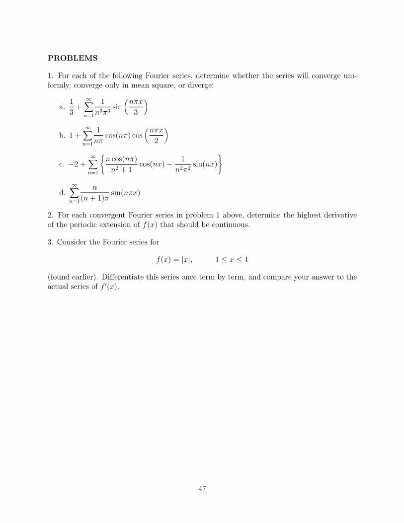
PROBLEMS

1. For each of the following Fourier series, determine whether the series will converge uni-formly, converge only in mean square, or diverge:

a.1

3+

∞∑n=1

1

n3π3sin

(nπx

3

)

b. 1 +∞∑

n=1

1

nπcos(nπ) cos

(nπx

2

)

c. −2 +∞∑

n=1

{n cos(nπ)

n2 + 1cos(nx)− 1

n2π2sin(nx)

}

d.∞∑

n=1

n

(n+ 1)πsin(nπx)

2. For each convergent Fourier series in problem 1 above, determine the highest derivativeof the periodic extension of f(x) that should be continuous.

3. Consider the Fourier series for

f(x) = |x|, −1 ≤ x ≤ 1

(found earlier). Differentiate this series once term by term, and compare your answer to theactual series of f ′(x).

47

2.5 Interpretation of the Fourier Coefficients

Thus far in this chapter, we have introduced the Fourier Series, learned how to calculate itscoefficients (an and bn) and seen how these coefficients relate to the convergence propertiesof the series. In this section we shall turn to a slightly different question - how should weinterpret the Fourier coefficients, i.e. what do they really represent? To do this, we shallneed the following trigonometric identity:

a cos(ωx) + b sin(ωx) = A cos(ωx− φ) = A cos(ω(x− δ))

whereA =

√a2 + b2

φ = tan−1

(b

a

)

δ =1

ωtan−1

(b

a

)=

1

ωφ

When using this identity, most engineering texts refer to φ as the phase angle, and δ as thedelay. (You should also note that, in order to use this identity both the sine and cosinemust have the same frequency, and you will need to handle the inverse tangent function“delicately” when a < 0.) This identity is easily verified with the aid of the standardidentity for the cosine of the difference of two angles:

cos(u− v) = cos(u) cos(v) + sin(u) sin(v)

If we then apply this identity to the nth term in the Fourier series (2.1.1), we have

an cos(nπx

L

)+ bn sin

(nπx

L

)= An cos

(nπx

L− φn

)= An cos

(nπ

L(x− δn)

)

where,

An =√a2

n + b2n

φn = tan−1

(bnan

)

δn =L

nπtan−1

(bnan

)

and then (using the delay form of the identity) write the Fourier series (2.1.1) in the equivalentrepresentation

f(x) = A0 +∞∑

n=1

An cos(nπ

L(x− δn)

),

(A0 =

a0

2

)(2.5.17)

48

Representing the Fourier series this way clearly emphasizes that the nature of the Fourierseries involves synthesizing a “complicated” periodic function as a combination of “pure” si-nusoidal terms (musically, these sinusoids would correspond to pure tones). Furthermore, An

now clearly represents the amplitude associated with the nth frequency component. More-over, since the power or energy in a pure sinusoid is proportional to the square of theamplitude, the An also affect the way in which the energy in a complex signal is distributedwithin the different frequencies. Thus, a plot of An (or A2

n) as a function of n (or of thefrequency - (n/2L)) represents essentially a “fingerprint” of the signal in terms of amplitude(energy). This amplitude plot is commonly referred to as the spectrum of the signal. (Notethat a complete characterization, or fingerprint of the signal would also require displaying thephase, φn as a function of n (or of frequency). A sample spectrum (for the signal computedas the first example in the first section) is shown below.

1 2 3 4 5 6 7 n

0.5

1.0

An

Figure 16: Spectrum of a Signal

The above interpretation can be further expanded by computing the average “energy”contained in a single period of a Fourier series signal, i.e.

1

2L

∫ L

−L[f(x)]2 dx

This integral is computed similarly to the derivation of (2.4.14), where, after squaring, mostof the terms integrate to zero by orthogonality, leaving:

1

2L

∫ L

−L[f(x)]2 dx = A2

0 +∞∑

n=1

1

2A2

n ≡a2

0

4+

∞∑n=1

{a2n + b2n}

2(2.5.18)

This result, which is frequently referred to as Parseval’s3 Theorem, has several ratherinteresting interpretations. First of all, it indicates that the power/energy in the differentfrequencies add independently to give the total energy. Stated another way, the variousdifferent frequencies in the series do not “spill over” or interact with each other. Changing theamplitude (or, it can also be shown, the phase) of a single frequency has no effect on the other

3Marc-Antoine Parseval des Chenes,see: http://turnbull.mcs.st-and.ac.uk/history/Mathematicians/Parseval.html

49

terms in the series. This property has some interesting applications in communications, sinceit implies that several independent signals could be sent down a single physical “channel,”and unambiguously decoded at the far end, provided a properly chosen set of differentfrequencies are used. In fact, one can show fairly simply that a more general concept oforthogonality than given by (3) is important for sending such signals, since a sufficientcondition for separation of the energy in any two signals∫ L

−L[f(x) + g(x)]2 dx =

∫ L

−L[f(x)]2 dx+

∫ L

−L[g(x)]2 dx

is, ∫ L

−Lf(x)g(x)dx = 0

A second conclusion which follows from (2.5.18) is that a necessary condition for mean-squareconvergence of a Fourier series is that the function, f(x), must have only finite energy onthe interval (−L,L).

The final conclusion which we shall develop from (2.5.18) describes “how good” an ap-proximation to f(x) is obtained by using just a partial Fourier series. Specifically, supposethat we wish to approximate an appropriate f(x) by just a finite trigonometric sum, i.e.

fapprox(x) =α0

2+

N∑n=1

{αn cos

(nπx

L

)+ βn sin

(nπx

L

)}(2.5.19)

where the αn and βn are, for the moment, any set of constants, not necessarily an and bn.Can we find a more accurate approximation than that given by the terms of the Fourierseries? To answer this question, we write out the complete Fourier series for f(x), and thensubtract the trigonometric approximation from it (term by term), we would find that theerror in approximating f(x) by (2.5.19) is:

e(x) = f(x)− fapprox(x)

=a0

2+

∞∑n=1

{an cos

(nπx

L

)+ bn sin

(nπx

L

)}

−α0

2−

N∑n=1

{αn cos

(nπx

L

)+ βn sin

(nπx

L

)}

=γ0

2+

∞∑n=1

{γn cos

(nπx

L

)+ ηn sin

(nπx

L

)}

where

γn =

{an − αn , 0 ≤ n ≤ Nan N < n

ηn =

{bn − βn , 1 ≤ n ≤ Nbn N < n

50

But since the error signal, e(x), is itself now just a Fourier series, with coefficients γn and ηn,we can apply (2.5.18) and compute the total energy in the error to be

∫ L

−L[e(x)]2 dx =

L

2

{γ2

0 +∞∑

n=1

{γ2

n + η2n

}}

Now, up until this point, we have not indicated how we should choose the coefficients inthe trigonometric approximation. But every term on the right in this last equation is non-negative. Therefore, the mean square error (i.e. the energy in the error signal) can beminimized only by making as many terms as possible in that equation equal to zero. Sincewe have no flexibility in the choice of an and bn, we cannot affect the values of γn and ηn

for n > N . This implies that we can minimize the error in our approximation (2.5.19) onlyby choosing

γn = 0 , 0 ≤ n ≤ N ,ηn = 0 , 1 ≤ n ,

or,αn = an , 0 ≤ n ≤ N ,βn = bn , 1 ≤ n ,

The importance of this result (which sometimes can get lost in the algebra) is that in orderto minimize the energy in the error of a trigonometric approximation, we must use preciselythe Fourier coefficients, an and bn, and therefore any purely trigonometric approximationcannot be improved from that given by the partial sum of a Fourier series without increasingthe number (N) of frequencies considered. This observation is summarized in the followingtheorem.

Theorem: The Fourier coefficients, an and bn, are optimum in the sense that theyprovide the best mean square approximation of a given function by a finite numberof trigonometric functions.

This theorem represents the last result we shall derive in this section. We have by nomeans exhausted all of the interpretations that can be applied to the Fourier coefficients, butwe have developed the primary ones that relate these coefficients to the amplitude, phase,and power at the different frequencies in the series. Lastly, we have shown that the Fouriercoefficients provide, in the mean square sense, the “best possible” choice for coefficients in atrigonometric expansion of a given function.

51

PROBLEMS

1. Plot the amplitude and phase as a function of frequency for each of the Fourier seriesfound for the problems in the first section of this chapter.

2. Prove Parseval’s Theorem (equation (2.5.18)). (Hint: first show

1

2L

∫ L

−L[f(x)]2 dx =

a20

4+

∞∑n=1

{a2n + b2n}

2

then use the definition of the An.)

52

2.6 The Complex Form of the Fourier Series

Although the reasons may not be apparent now, it is often advantageous to express the basicconcepts of Fourier series in terms of complex variables. Such an alternative formulation isclearly possible since the relations

eix = cos(x) + i sin(x) ,

cos(x) =eix + e−ix

2

sin(x) =eix − e−ix

2i

allow conversion between the normal, real-valued trigonometric forms and the complex ex-ponential form. (No apology will be made here for the mathematician’s use of the symbol irather than the engineer’s j to stand for

√−1.)We could now convert (2.1.1) to complex form by replacing the trigonometric functions

there with the above equivalent complex exponential forms, and then algebraically regroupthe terms. This substitution will clearly produce complex exponential terms of the form

einπx/L

for all positive and negative values of n, i.e. for all values between plus and minus infinity,and therefore reduce (2.1.1) to an expression like:

f(x) =∞∑

n=−∞cne

inπx/L (2.6.20)

where the cn are (probably complex) constants. (Note that the n = 0 term of this seriesmust represent the constant (DC) term of the original signal.) As already noted, we coulddetermine the values for cn by algebraically regrouping the terms, after replacing the trigono-metric functions by their equivalent complex exponentials. But there is an easier way, whichalso happens to be theoretically more pleasant!

Recall how we derived the coefficients in the original, real-valued Fourier series. Wemultiplied both sides of the series equation by just one of the trigonometric functions, andthen integrated and applied the orthogonality integrals. So why not try a similar approachhere?

With this general approach in mind, let k stand for some fixed, but arbitrary integer, andmultiply both sides of (2.6.20) by eikπx/L, and integrate from −L to L. After interchangingthe summation and integration, this yields

∫ L

−Lf(x)eikπx/Ldx =

∞∑n=−∞

cn

∫ L

−Lei(k+n)πx/Ldx

But now, direct computation will show that the complex exponentials also obey an orthog-onality relation ∫ L

−Lei(k+n)πx/Ldx =

{0 , n = −k2L , n = −k (2.6.21)

53

Therefore, the above equation simplifies to

∫ L

−Lf(x)eikπx/Ldx = 2L c−k

or, replacing k by −n on both sides,

cn =1

2L

∫ L

−Lf(x)e−inπx/Ldx (2.6.22)

With this formula for the cn, we can now express the complex exponent in terms of ordinarytrigonometric functions, and use the fact that the integral of a sum in the sum of the integrals,to rewrite (2.6.22) as

cn =1

2L

{∫ L

−Lf(x) cos

(nπx

L

)dx− i

∫ L

−Lf(x) sin

(nπx

L

)dx

}

=1

2{an − ibn} , n > 0

(2.6.23)

where an and bn are, of course, just the standard Fourier coefficients as given by (2.2.5)-(2.2.6). This shows, as we had expected, the cn are complex. Furthermore, we can noweasily relate them to the An and φn that appeared when we converted the real-valued Fourierseries to amplitude-phase form. Specifically, we see from (2.6.23) that:

|cn| = 12An

arg(cn) = − tan−1

(bnan

)= −φn = −nπ

Lδn

(Note also that, provided f(x) is real, c−n = c∗n, i.e. c−n is the complex conjugate of cn.Thus |c−n| = 1

2An and arg(c−n) = φn.) Thus the energy in any single frequency in the real

series is split equally between the two (one positive and one negative) respective complexfrequencies.

From the above, it is clear that one could plot |cn| as a function of n (for −∞ < n <∞)and, except for the fact that the amplitude associated with the each real frequency (nπ/L)is equally divided between the two complex frequencies, we obtain the identical informationthat would be obtained from plotting the real-valued amplitude spectrum described earlier.In fact, especially in applications in electrical engineering and signal processing, the com-plex amplitude spectrum is customarily used instead of the real-valued amplitude spectrum.There are many reasons for this, including both the relative ease of working with complexnumbers, especially when multiplications are involved, and the often powerful insights thatare possible using the complex plane representation.

At this time, however, we will only consider the complex Fourier series as simply analternative to the real-valued representation, although we shall return to it later when wediscuss Fourier transforms.

54

PROBLEMS

1. Find the complex Fourier series for each of the following functions:

a. f(x) = x,−3 ≤ x ≤ 3 , f(x+ 6) = f(x)

b. f(x) =

{0 , −1 < x < 01 , 0 < x < 1

f(x+ 2) = f(x)

2. Plot the complex amplitude spectrum for each of the series found in problem 1 above.

3. Show that if we use T0 for the period of a signal, rather than 2L, the formula for thecomplex Fourier series coefficients reduces to

cn =2

T0

∫ T0/2

−T0/2f(x)e−2inπx/T0dx

4. Using the complex form of the Fourier series, prove the following form of Parseval’stheorem

1

2L

∫ L

−L|f(x)|2 dx =

∞∑n=−∞

|cn|2

(Hint: Show

|f(x)|2 = f(x)f(x)∗ =

[ ∞∑n=−∞

cneinπx/L

] [ ∞∑m=−∞

c∗me−imπx/L

]

=∞∑

n=−∞

∞∑m=−∞

[cnc

∗me

i(n−m)πx/L],

then integrate.)

55

2.7 Fourier Series and Ordinary Differential Equations

Thus far, we have concentrated on developing the basic concepts of Fourier Series themselves.There are many other interesting questions about these series, which we might pursue. Thefirst one we shall study is where Fourier Series “fit” in the scheme of ordinary differentialequations.

Consider the ordinary differential equation,

py′′ + qy′ + ry = f(x) (2.7.24)

where p, q, and r may be any constants, and f(x) is some general periodic function,i.e. f(x+ 2L) = f(x), but f(x) need not be a simple sine or cosine. (For example, f(x)might look like Figure 17.) We now wish to ask the question - are any of the ordinary dif-ferential equations methods which you should have seen prior to Fourier Series (variation ofparameters, Laplace transforms, or undetermined coefficients) well-suited for this problem?

We know that variation of parameters will produce a solution to this problem. But,you should recall that, besides being usually the least efficient method to produce non-homogenous solutions (when a viable choice exists), variation of parameters produces asolution in terms of integrals which involve the forcing function. But, as we have seen inour earlier computations of Fourier coefficients, evaluating an integral involving a piecewisesmooth f(x) normally involves splitting the integral into several parts. For example, forthe f(x) given in Figure 17, if e−x were a homogeneous solution,

−4 −3 −2 −1 0 1 2 3 4 5−0.2

0

0.2

0.4

0.6

0.8

1

f(x)

x

x 2−x

x−4

Figure 17: A Typical Periodic Function

variation of parameters would require computing integrals like

∫ 4.5

0e−xf(x)dx

which, due to definition of f(x), would have to be expressed as,

∫ 1

0xe−xdx+

∫ 2

1(2− x)e−xdx+

∫ 4.5

4(x− 4)e−xdx

56

and would actually require three integrations. Such behavior could, in general, make theevaluation of variation of parameters integrals a computational morass for this class of prob-lems. Thus, if at all possible, we would like to avoid variation of parameters here.

The utility of the Laplace transform in this class of problems is affected by the fact thatmost “interesting” periodic, non-sinusoidal, functions have jump discontinuities in eitherthe function or one of its derivatives. (The f(x) graphed above has discontinuities in f ′(x)at each of the sharp corners.) Furthermore, it is well-known from the study of Laplacetransforms that each such jump discontinuity in f(x) will produce an e−sc type term in thetransform, where x = c is the location of the discontinuity. But with a periodic function,if there is one discontinuity, there must be an infinite number. Therefore, for example, thetransform of a square wave (see Fig. 18)

1 2 3 4 5

1

Figure 18: Square Wave

would have an infinite number of different e−sc type terms. (Specifically, you should be ableto show for this f(x) :

F (s) =1

s+

∞∑n=1

(−1)n e−ns

s

But, since using the Laplace transform to solve the ordinary differential equation (2.7.24)involves a term of the form

F (s)

as2 + bs+ c

it is clear that if F (s) contains an infinite number of different e−sc type terms, you will,at least in principle, have to apply the Laplace inverse (including the Heaviside shift) aninfinite number of different times. Like variation of parameters, this is possible, at least intheory, but it normally becomes computationally cumbersome, and leads to results oftentoo complicated to provide any insight into the real properties of the solution. Thus, weconclude that the Laplace transform is also not a particularly suitable method for this classof problems.

With neither variation of parameters nor the Laplace transform seeming to be an es-pecially attractive method for this class of problems, we turn to the last of the standardmethods studied with ordinary differential equation methods - undetermined coefficients.Undetermined coefficients, however, can be used only when the forcing function, f(x), meets

57

fairly stringent criteria. Specifically, the only periodic functions for which the method ap-plies are sines, cosines, and linear combinations of these. Functions such as that shown inFigure 18, at first, do not appear to meet this criterion.

However, we now know that this (and similar) f(x) can be written as a combinationof sines and cosines (specifically in the form of a Fourier Series). Furthermore, since theordinary differential equation is linear, we know the Principle of Superposition holds. Thus,we claim that a particular solution to

py′′ + qy′ + ry = f(x) =a0

2+

∞∑n=1

{an cos

(nπx

L

)+ bn sin

(nπx

L

)}

is

yp(x) = yp0(x) +∞∑

n=1

ypn(x)

wherepy′′p0

+ qy′p0+ ryp0 =

a0

2

py′′pn+ qy′pn

+ rypn = an cos(nπx

L

)+ bn sin

(nπx

L

), n = 1, 2, . . .

It should be obvious now that not only can undetermined coefficients be applied to eachof these equations, but that in most cases a general expression for yp(x) can be obtained byassuming,

ypn(x) = αn cos(nπx

L

)+ βn sin

(nπx

L

), n = 1, 2, . . .

(Note that under some special values of p, q, and r, this form might not be appropriatefor one (and only one) value of n.) In fact, if p, q and r are all positive, then we can provethat a particular solution will always have the form

yp(x) =α0

2+

∞∑n=1

{αn cos

(nπx

L

)+ βn sin

(nπx

L

)}

where,

yp0 =a0

2r

provided only that the Fourier Series for f(x) converges.Thus we conclude that the main value of Fourier Series in ordinary differential equations

is that it allows us to decompose complicated periodic forcing functions into a linear com-bination of sines and cosines, thus permitting the particular solution to a linear, constantcoefficient equation to be obtained by using undetermined coefficients and the Principle ofSuperposition. (As we shall shortly see, the role of Fourier Series in partial differentialequations is even more crucial.)

58

PROBLEM

1. Use Fourier series to construct a non-homogeneous solution to the ordinary differentialequations:

y′′ + 2y′ + y = f(x),

where:

f(x) =

{x , 0 ≤ x < 1

2− x , 1 ≤ x ≤ 2

f(x+ 2) = f(x)

59

2.8 Fourier Series and Digital Data Transmission

The emergence of so-called digital signal processing has had a major impact on electronics,and especially communications. In its simplest form, a digital signal consists of a sequenceof ones and zeros, for example,

1 1 0 1 0 1 0 0 .

(You may recognize this as the binary representation of the number 212.) Physically, ontransmission lines, a “1” might be represented by a unit voltage being present, and a “0” byno voltage. Thus, the above sample signal might be transmitted, in time sequence, as shownin Figure 19.

t

+v

1 2 3 4 5 6 7

Figure 19: A Transmitted Digital Signal

A major concern of communications engineers is how much will such a signal be altered,distorted or degraded as it passes through both circuits and transmission lines. A verysimple model that nevertheless illustrates two major effects can be developed by using someelementary concepts from Fourier series and ordinary differential equations to analyze theresponse of the circuit shown in Figure 20 to an applied digital test signal.

This circuit consists of a resistor, capacitor, inductor and input voltage source, E(t). Theoutput is assumed to occur by measuring the voltage across the resistor (which is often calledthe load). If Q(t) and I(t) denote, respectively, the charge on capacitor and the current inthe circuit at time t, then Q(t) and I(t) are related by:

I(t) =d

dt[Q(t)] =

dQ

dt. (2.8.25)

The relations between these variables and the instantaneous voltages across the resistor,capacitor and inductor are given, respectively, by

VR = RI , VC = Q/C , and VL = LdI

dt.

60

Figure 20: A Simple Circuit

Thus, if we apply Kirchhoff’s Law, which states that the sum of the voltage drops aroundthe circuit components must equal the applied (source) voltage, we have

LdI

dt+RI +

1

CQ = E(t) ,

or

Ld2Q

dt2+R

dQ

dt+

1

CQ = E(t) . (2.8.26)

Suppose now that this circuit is subjected to an E(t) made up of the periodic train of “0”sand “1”s shown in Figure 21.

−5 −4 −3 −2 −1 0 1 2 3 4 50

0.2

0.4

0.6

0.8

1

t

E(t)

Figure 21: A Periodic Digital Test Signal

Our principal interest is how closely does the voltage across R follows this pattern, or equiv-alently, could another electrical device attached to R reasonably infer what the original testsignal was based on the voltages observed across R? To determine this, we first assume that

61

we look at the circuit after all transients have effectively dropped to zero, i.e. when onlythe steady-state solution persists. The input signal, E(t), can be represented by the Fourierseries:

E(t) =a0

2+

∞∑n=1

{an cos(nπt) + bn sin(nπt)}

=1

2+

∞∑n=1

(1− cos(nπ))

nπsin(nπt) ,

(2.8.27)

where the an and bn are determined by the usual formulae,

an =∫ 1

−1E(t) cos(nπt) dt ,

bn =∫ 1

−1E(t) sin(nπt) dt .

Now, since E(t) is thus a sum (albeit an infinite one) of forcing terms, and since the dif-ferential equation (2.8.26) is linear, we invoke the Principle of Superposition, and claim thesteady-state solution should have the form

Qss(t) = Q0(t) +∞∑

n=1

Qn(t) ,

where each Qn(t) is the response to a single frequency in the forcing voltage, E(t). Thus,

Ld2Q0

dt2+R

dQ0

dt+

1

CQ0 =

1

2,

and

Ld2Qn

dt2+R

dQn

dt+

1

CQn =

(1− cos(nπ))

nπsin(nπt) , n = 1, 2, 3, . . . .

(2.8.28)

(In reality, this is a non-trivial extension of the usual principle of superposition. The forcingfunction is not a finite sum, and the whole structure of infinite series arises precisely becausenot all properties that hold for finite sums also hold for infinite series. Rigorous justificationof this approach at this point would require a detailed analysis of the rates of convergenceof the series involved. Fortunately, in the case of Fourier series, such an investigation willalmost always show that this method is valid.)

Provided R > 0 , there will be no undamped resonance, and therefore, by the method ofUndetermined Coefficients, we see that the Qn(t) will have the form

Q0(t) =α0

2,

Qn(t) = αn cos(nπt) + βn sin(nπt) , n = 1, 2, 3, . . . ,

(2.8.29)

62

where αn and βn are constants. Substitution of the above expressions into (2.8.28), followedby equating the coefficients of like terms, yields

α0 = C ,

and

− [n2π2L− (1/C)]αn + nπRβn = 0 ,

−nπRαn − [n2π2L− (1/C)]βn =(1− cos(nπ))

nπ.

(2.8.30)

Solution of the system of two equations in two unknowns in (2.8.30) yields

αn =(1− cos(nπ))

nπ

[−nπR][(n2π2L− 1

C

)2+ n2π2R2

] ,

βn =(1− cos(nπ))

nπ

[− (n2π2L− (1/C))][(n2π2L− 1

C

)2+ n2π2R2

] .

(2.8.31)

Thus

Qss(t) =C

2+

∞∑n=1

(1− cos(nπ))[−nπR cos(nπt)− (n2π2L− (1/C)) sin(nπt)]

nπ[(n2π2L− 1

C

)2+ n2π2R2

] . (2.8.32)

Recall, however, what we are really interested in is the voltage across the (load) resis-tor, R. But, according to our basic equations, the steady-state current in the circuit shouldbe just the time derivative of the steady-state charge on the capacitor, i.e.

I(t) =dQss

dt,

and, therefore, by Ohm’s Law, the steady-state voltage across the resistor is then given by

Vss(t) = RdQss

dt.

Differentiating Qss(t) as given by (2.8.32) term by term (which, if we were mathematicallyprecise, would again require consideration of the rates of convergence of the series involved)and then multiplying by the resistance, yields

Vss(t) = R∞∑

n=1

(1− cos(nπ))[nπR sin(nπt)− (n2π2L− (1/C)) cos(nπt)][(n2π2L− 1

C

)2+ n2π2R2

] . (2.8.33)

63

Standard trigonometric identities4 can then be used to reduce this to

Vss(t) =∞∑

n=1

(1− cos(nπ))

nπAn sin(nπt− φn) , (2.8.34)

where

An =nπR√[(

n2π2L− 1C

)2+ n2π2R2

] ,

and

φn = tan−1

[(n2π2L− (1/C))

nπR

].

(2.8.35)

Careful examination of this representation for Vss(t) yields some very valuable insightsinto the problems of digital communications, starting with the observation that there arestriking similarities between the series for the output, Vss(t), as given by (2.8.34), and theseries for the input, E(t), as given by (2.8.27). However, there are also two striking differ-ences:

(1) Each sine term in Vss(t) has an amplitude equal to

(1− cos(nπ))

nπAn , (2.8.36)

which is precisely An times the amplitude of the corresponding sine term (i.e. fre-quency) in the input.(2) Each sine term in the output has undergone a phase shift, due to the φn term, relative

to the corresponding input term.

Communications engineers would describe these two effects as amplitude distortion andphase (or delay) distortion, respectively. We shall see shortly exactly why these effects distortthe signal, but first we need to more explicitly define the term “distortion” and illustrateour definition with some simple examples.

By distortion, we shall mean any change that serves to alter the fundamental shape of asignal, i.e. a change such that the original signal cannot be recovered by any combination ofonly the following techniques:

4The identity is:

A sinΘ−B cosΘ =√

A2 + B2

[A√

A2 + B2sin Θ− B√

A2 + B2cosΘ

]

= R sin(Θ− φ)

whereR =

√A2 + B2 , sin φ =

B√A2 + B2

, and cosφ =A√

A2 + B2.

64

(1) simple amplification (i.e. change of scale of the vertical axis, or, equivalently,multiplication of the function by a constant)5,

(2) insertion of a DC bias (i.e. shift up or down of the horizontal (t) axis, or,equivalently, addition of a constant),

(3) a simple time delay (i.e. a shift right or left of the location of the vertical axis,or, equivalently, replacing t by (t− c)).6Thus, for example, figures 22(a)-(c) do not represent distortion of the original E(t), since

E(t) can be recovered, respectively, by amplification by a factor (gain) of 2, a time shift of(1/2), and a DC bias of (1/4). Figure 22(d), however, does represent a distortion, since thereis no way to restore its form to that of E(t) by the above operations.

−1 0 1 2 3 4 5−0.5

0

0.5

1

t

E(t)

−1 0 1 2 3 4 5−0.5

0

0.5

1

t

E(t)

−1 0 1 2 3 4 5−0.5

0

0.5

1

t

E(t)

0 2 4 6−0.5

0

0.5

1

1.5

Figure 22: Undistorted and Distorted Signals

It is relatively easy to prove that if a signal is composed of more than one frequency(Fourier series term) and if any one component frequency (term) is multiplied by a constant,then, to remain undistorted, every component must be multiplied by the same factor. Asimilar conclusion can also be shown to be valid for time delays of a signal composed of a

5The term “amplification” is used here in the general sense which includes cases where the “amplified”signal is actually weaker than the original signal. The latter cases is commonly referred to in engineering as“amplification with a gain less than one.”

6With periodic functions, one must be slightly careful to ensure that the delays are truly different, sincea delay of an integral number of periods is, physically, undetectable.

65

sum of terms, i.e. any effect which serves to introduce different delays into different termswill distort the resulting signal, just as would “out of step” marchers in a parade.

With these ideas in mind, return to (2.8.36). Note that for each value of n, An repre-sents the factor by which the amplitude of that frequency component in the input has beenamplified. As is obvious from (2.8.35), An is not constant with respect to different valuesof n. Thus to restore the amplitudes in the output to their original (input) values wouldrequire multiplication of each term by a different amount, i .e. different amplification ateach frequency. Since, as we discussed above, this is not the same as amplifying the outputsignal by a single factor, we conclude that Vss(t) is a distorted version of E(t). Since thisdistortion arises due to changes in the relative amplitudes at different frequencies, it is aptlytermed amplitude distortion.

However, distortion of the relative amplitudes is not the only source of distortion inVss(t). Also observe that, since Vss(t) (2.8.34) can be written

Vss(t) =∞∑

n=1

(1− cos(nπ))

nπAn sin

(nπ

(t− 1

nπφn

)), (2.8.37)

the nth frequency in Vss(t) is shifted, relative to the corresponding frequency in the input.Here, a little careful analysis is required, for if φn in (2.8.34) is positive, then each termin Vss(t) is advanced compared to the same term in E(t). Equivalently, a negative valueof φn corresponds to a delay in the response. Therefore, the nth frequency in Vss(t) isdelayed, relative to the corresponding frequency in E(t), by a time interval equal to

tdn = − 1

nπφn

= − 1

nπtan−1

[(n2π2L− (1/C))

nπR

].

(2.8.38)

But this implies that, unless tdn is constant, the different frequencies in the output signalhave been delayed selectively, i.e. by different amounts. But, as defined above, tdn is clearlynot constant. Thus the output signal can be restored to its original form only by insertingan additional different delay at each frequency, not a single delay at all frequencies. As withselective amplification, selective delay must distort the signal, and hence we conclude thatany non-constant φn also distort Vss(t). This type of distortion, as we commented above iscommonly referred to as phase or delay distortion. (In transmission through physical media,such as in optical communications, a similar effect is observed. That effect is commonlyattributed to a non-constant index of refraction, which causes slightly different transmissionvelocities at different frequencies, or slightly different transmission path lengths at differentfrequencies. When encountered in this context, the effect is often referred to as dispersion.)

(We close this part of the discussion by noting that a mathematician would more likelyconclude that Vss(t) is distorted by noting that for large n, the coefficients in (2.8.33)and (2.8.34) obey:

(1− cos(nπ))

nπAn = O

(1

n2

),

66

and hence the series for Vss(t) must converge uniformly (by the Weirstrauss M-test). Astandard result from the study of infinite series then guarantees that Vss(t) is a continuousfunction, and hence cannot have the sharp “jumps” that characterize E(t). Thus, clearly,the “shape” of Vss(t) cannot be the same as that of E(t), and hence Vss(t) is a distortion ofE(t).)

Observe, for a moment, what we have just done. We have studied the possible effects ofthe circuit on the original input signal by analyzing how each of the individual frequenciesin that signal are affected. This is what we call a frequency domain analysis! This methodis almost certainly the best, if not the only way to understand why the output signal maynot “look” exactly like the input.

How much or little effect distortion can have on a signal can be graphically demonstratedby two carefully chosen numerical examples. Consider first the case

L = 0.02 , C = 5.00 and R = 0.75 .

0 5 10 15 200

0.2

0.4

0.6

0.8

1

n

An

0 5 10 15 20

0

0.2

0.4

0.6

0.8

1

n

t dn

−2 −1 0 1 2

−0.6

−0.4

−0.2

0

0.2

0.4

0.6

t

Vss

Figure 23: First Sample Output

The graphs of An and tdn for these specific values of L, R and C are shown at Fig-ures 23(a)-(b), respectively. (Note that in these figures An and tdn are shown for all values,not only the integer (n) values, although when Vss(t) is computed, only the values at theinteger points will be used.) The curve for An shows noticeable attenuation at higher fre-quencies, although for n < 20 the attenuation never exceeds 50%. (Engineers would refer tothis as the 3 dB point.) The curve for tdn appears almost flat for n > 1, suggesting almost

67

no noticeable delay distortion should occur in this example. Computation shows that themaximum difference between the delays encountered by different frequencies is:

td1 − td5 = 0.0185

which is less than 1% of one period. Therefore, with neither the amplitude nor delay distor-tion seeming especially severe, we might expect the output across R would not be too badlydistorted. This is, in fact, the case. Figure 23(c) shows Vss(t), computed for the values ofL, R, and C given above by taking a sufficient number of terms in a partial sum of (2.8.33).Note that except for the DC shift of 1/2 unit, it is a fairly recognizable replica of the originalsignal. Note that Figure 23(c), since it represents the sum of the series, is a time domainview of the phenomenon, while, as discussed above, Figures 23(a) and 23(b) are frequencydomain views.)

Lastly, consider the example given by:

L = 0.16 , C = 0.01 and R = 0.75 .

0 5 10 15 200

0.2

0.4

0.6

0.8

1

n

An

0 5 10 15 20−0.2

0

0.2

0.4

0.6

0.8

1

n

t dn

−1 −0.5 0 0.5 1−0.2

−0.1

0

0.1

0.2

t

Vss

Figure 24: Second Sample Output

The graphs for An, and tdn for these values are shown in figures 24(a)-(b), respectively.(Again, the figures plot non-integer values as well as integer values.) Observe that in thiscase the curves are nowhere near as constant as the corresponding curves in the previousexample. The curve for An shows that frequencies with n < 6 and n > 12 will be severely

68

attenuated. Furthermore, the maximum difference between delays at different frequencies inthis case is approximately 0.40, or a factor of twenty greater than in the previous example.Thus, we would expect the output from this circuit to be noticeably more distorted than inprevious case. As shown by Figure 24(c), it is. In fact, the time domain output representedby Figure 24(c) is so badly distorted that it would be almost impossible to determine whatthe original (input) signal had been by observing the output. Of course, that would makethe second circuit almost useless for communicating the original signal. In contrast, sincethe output from the first circuit is only slightly distorted from the original input, that circuitwould be reasonably appropriate for transmitting this particular signal.

This example demonstrates how the ability of Fourier series to decompose complicated,periodic (time domain) signals into “pure” (frequency domain) sines and cosines allows acommunications engineer/designer to analyze the distortion introduced into a digital signalas it passes through a simple circuit, and to compute the (distorted) output signal from thatsame circuit. This is but one aspect of the power of Fourier series - the ability to providesimple analysis of the response of linear systems.

69

3 The One-Dimensional Wave Equation

3.1 Introduction

One of the principal applications of Fourier series is to the solution of partial differentialequations. Such equations are fundamental to both the physical sciences and to engineering,and describe a tremendous variety of different and important physical processes. In thischapter, we shall study the application of Fourier series to primarily one partial differentialequation, the so-called wave equation. Our intent in this study will be two fold - not only toinvestigate the mechanics of solving these problems with Fourier series , but also to observeand interpret the physical insights contained in these solutions. As part of these insights,we shall see that the wave equation shares the same dual time-domain, frequency-domainnature that we observed earlier in the Fourier series itself and in the application of FourierSeries to the solution of ordinary differential equations.

The wave equation is really a mathematical model - a set of equations that describesome idealized , simplified version of reality. Such mathematical models are common inapplications, and generally arise when one tries to include only the most important inter-relationships, forces, etc. In modeling most physical processes, we start by identifying theprimary forces and relationships. Then, we generally apply various conservation laws tothe identified forces to produce the governing equations. Finally, once these equations havebeen solved, we must show that our solutions accurately reflect the observed actual physicalbehavior before we can consider the model to be valid. As we proceed with our study of thewave equation, we will endeavor to point out these various aspects of the modeling processwhen they occur.

3.2 The One-Dimensional Wave Equation

The physical prototype for the wave equation is a thin, tightly stretched elastic string, suchas a violin string or a guitar string. These strings are usually wound around some type ofpeg to produce an extremely strong internal tension. (The magnitude of this tension can bereadily appreciated by anyone who has seen a guitar string break while being played.)

The first step in deriving the mathematical model is to identify what we believe are theprimary forces and interactions, or, equivalently, to assume which terms and interactions canbe neglected. For our model, we assume that the string is extremely thin in comparison to itslength, and so tightly stretched that at rest (equilibrium) it does not sag, but lies perfectlyhorizontal. We further assume that all motion of the string is purely one-dimensional (inthe vertical direction), that any displacements from equilibrium of the string and any anglesbetween the string and the horizontal are small. (Any readers who are skeptical about theseassumptions should look closely at a plucked guitar string - the displacement is virtuallyimperceptible. In fact, a reasonable scale for Figure 25 would be a meter along the hori-zontal axis, and a millimeter in the vertical!) To emphasize that the motion can vary withboth time and position, we shall denote the vertical displacement from equilibrium by thesymbol u(x, t).

We shall also assume that the original cross-sectional area and density of the string

70

Figure 25: An Elastic String

were uniform (constant), and that any changes in cross-section or density resulting fromstretching of the string during its motion are negligible. (The latter part of this assumptionensures consistency with our earlier assumption of extremely small vertical displacements.)Therefore the linear density (mass per unit length) of the string will remain constant. Weshall use the symbol ρ to represent this density. Finally, we assume that there is a uniformtension, which we shall denote by τ , throughout the length of the string.

By now, you may feel as if it seems like we are making a lot of assumptions. In a sense,perhaps we are. However, as we observed above, there is effectively one “acid test” forwhether these assumptions are in fact reasonable. This test is whether or not the values ofthe mathematical solutions to the equations that result from the model assumptions agreewith the actually observed and measured physical motion of such strings. If these values agreewell with “reality,” then we accept the model as being a relatively accurate representation ofreality. If, however, the model leads to solutions that do not agree with observed phenomena,then we would have to go back to our fundamental assumptions and ask - “What have wemissed? What have we ignored? What have we neglected?” - because apparently somethingimportant is going on which we have not captured.

Once we have identified the basic assumptions in this, or any similar problem, the nextstep is to set up the complete description of all the interior forces at work. To do this, weconsider an idealized segment located at some arbitrary position in the interior of the string(Figure 26). The segment is assumed to be of a “small” length, denoted by ∆x, and locatedbetween x and x+ ∆x.

Assuming some basic background in physics on the reader’s part, we now proceed toidentify the possible forces that could act on this small segment.

Since we have assumed there is no motion except in the vertical direction, we will notanalyze any forces in the x or z direction, and concentrate on only those in the vertical.Figure 26 clearly seems to indicate that there are at most three possible forces acting on

71

Figure 26: A Small Segment of the String

this segment - a tension force exerted on the left end by the neighboring segment of stringthere, another similar tension force exerted on the right end, and then, possibly, some kindof external (commonly called body) force. As the figure implies, this body force, if any,effectively acts through the center of mass of the segment, which, since we have assumedthe string has a uniform density, coincides with its geometrical center. (Typical body forcesarise from gravity (which we have already effectively neglected here by assuming the stringlies flat at equilibrium), magnetic fields, damping due to air friction, etc.) In our model, weshall simply represent acceleration due to this body force by g(x + 1

2∆x, t). Note that this

representation emphasized not only the fact that the force acts through the center of mass,but also that such forces generally vary with both time and position. (Some body forcesin fact, may also vary with the displacement or vertical velocity of the string, i.e. have theform g(x + 1

2∆x, t, u, ∂u

∂t).) However, since we have also assumed a constant linear density

and no effective lengthening of the string, the mass of our small segment is ρ∆x, and so theresulting vertical force on the segment due to body forces is represented by

ρg(x+ 12∆x, t)∆x .

We turn next to the tension forces exerted on the segment by its neighboring segments.We represent these forces, which must lie along the tangents to the string, by two vectorsof equal magnitude, tangent at the left and right ends of the segment. (The fact that themagnitudes are equal is not accidental, but is a direct consequence of our earlier modelassumptions that the internal tension is uniform, that there is no net horizontal motion andthat the angles between the string and the horizontal are small.) However, if the string hasany curvature, the angles at the right and left ends, while small, will generally not be equal.Therefore, even though the magnitudes of the two tension forces are equal, their directionswill generally not be identical, and this will result in a net vertical force component due totension. The normal rules for decomposing vectors into their components give the vertical

72

components of the tension at the left and right hand ends, respectively, as

−τ sin(θL) and τ sin(θR) ,

and therefore their sum,τ sin(θR)− τ sin(θL) ,

represents the net vertical tension on this segment. (You should understand that since theseare components of vectors, the negative sign associated with the left hand component ismandatory to ensure consistency with our convention that the upward vertical direction ispositive.)

But now we return to our assumptions that the displacements and angles (θL and θR)are small. Therefore, mathematically,

θi ≈ sin(θi) ≈ tan(θi) , i = L,R ,

and we can now express the net vertical force due to tension as essentially equal to

τ tan(θR)− τ tan(θL) .

However, a fundamental result from the calculus is that the slope of the tangent line to acurve is also precisely the tangent of the angle between the curve and the horizontal axis,and is given by the value of the first derivative of the equation for the curve at that point.Therefore,

tan(θR) =∂u

∂x(x+ ∆x, t) and tan(θL) =

∂u

∂x(x, t) .

(Note we must use partial derivatives here, since u(x, t) is a function of two variables. Furthernote that the slope is given by the partial with respect to x, while the vertical velocity wouldbe given by the partial with respect to t.

Combining all of these components yields that the net vertical force acting on the smallsegment of the string is

τ

{∂u

∂x(x+ ∆x, t)− ∂u

∂x(x, t)

}+ ρg(x+ 1

2∆x, t) ∆x

But, if this net force is not zero, then, according to Newton’s second law of motion, thesegment will experience a proportional vertical acceleration, i.e. F = ma. This is ourconservation law! (You may recall from your basic college physics courses that Newton’ssecond law is equivalent to conservation of momentum.) Since we already know the massof this segment (ρ∆x), and since the vertical acceleration (computed at the center of massof the segment) is nothing more that the second derivative of position with respect to time,i.e.,

∂2u

∂t2(x+ 1

2∆x, t) ,

then Newton’s second law reduces to

ρ∂2u

∂t2(x+ 1

2∆x, t)∆x = τ

{∂u

∂x(x+ ∆x, t)− ∂u

∂x(x, t)

}+ ρg(x+ 1

2∆x, t) ∆x .

73

This, of course, being a mathematics text and written by a mathematician, there is no waywe can not succumb to the temptation to divide by ∆x, yielding

ρ∂2u

∂t2(x+ 1

2∆x, t) = τ

{∂u∂x

(x+ ∆x, t)− ∂u∂x

(x, t)

∆x

}+ ρg(x+ 1

2∆x, t) ,

and then let ∆x approach zero. (After all, isn’t this what every mathematics book does?)Thus we have

ρ∂2u

∂t2(x, t) = τ lim

∆x→0

[∂u∂x

(x+ ∆x, t)− ∂u∂x

(x, t)

∆x

]+ ρg(x, t) .

But now, wait! That limit should look familiar. It’s nothing more, basically, than thedefinition of a partial derivative - specifically the partial derivative of ∂u/∂x with respectto x, i.e. exactly what we mean by

∂2u

∂x2(x, t) .

Putting all of these pieces together, we have,

ρ∂2u

∂t2(x, t) = τ

∂2u

∂x2(x, t) + ρg(x, t) ,

the writing of which we shall now simplify by dividing through by ρ and dropping the explicitreference to x and t in u, to yield

∂2u

∂t2=τ

ρ

∂2u

∂x2+ g(x, t) . (3.2.1)

There is one final simplification we shall use. Since τ and ρ are positive constants, then so istheir ratio, τ/ρ, and we therefore shall replace the ratio by the single value c2. The square isdeliberately used to unequivocally emphasize the positive character of the ratio. (It will alsomake the algebra a lot simpler later on!) Thus, we finally have the one-dimensional waveequation:

∂2u

∂t2= c2

∂2u

∂x2+ g(x, t) . (3.2.2)

There is one further, minor simplification that we shall mention. Partial derivatives arefrequently represented by subscripts, instead of with the ratio notation, except in caseswhere subscripts would be ambiguous. Thus, for example, many texts will write

ux instead of∂u

∂x, etc.

In this notation, which we shall frequently use, the one-dimensional wave equation wouldthen be written

utt = c2uxx + g(x, t) . (3.2.3)

74

PROBLEMS

1. Show that if a uniform, thin, tightly stretched elastic string is acted upon by no forcesother than internal tension and an external air resistance proportional to the vertical velocity,then Newton’s second law leads to a partial differential equation of the form:

∂2u

∂t2+ κd

∂u

∂t=τ

ρ

∂2u

∂x2,

where κd is some positive constant of proportionality.

2. Show that if a uniform, thin, tightly stretched elastic string is acted upon by no forcesother than internal tension and an external spring-like restoring force proportional to thevertical displacement, then Newton’s second law leads to a partial differential equation ofthe form:

∂2u

∂t2=τ

ρ

∂2u

∂x2− κsu ,

where κs is some positive constant of proportionality.

75

3.3 Boundary Conditions

Our just-completed derivation of the one-dimensional wave equation includes, however, onecrucial restriction. It arose from considering an internal segment of the string, and reallyexpresses only the physics that are occurring inside the string. But guitar strings don’tstretch on forever - they’re usually only two or three feet long at best! They have ends!Physically, these ends, which we have denoted as x = 0 and x = L in our model, representlocations where the physics of the process change, i.e. locations where the internal physics nolonger validly describe what is occurring. Mathematically, at the ends and beyond, the basicgoverning partial differential equation ceases to hold true. (In other words, to be preciselycorrect, we really should have written (3.2.3) as

utt = c2uxx + g(x, t) , 0 < x < L .

Therefore, in order to completely specify our model, we must also derive mathematicalequations which correctly express the physics that are occurring at these ends.

The derivation of the mathematical conditions at the ends turns out to be a bit moreinvolved than was the derivation of the equation for the interior physics, primarily because,instead of the single basic internal process just studied, there are a fairly large numberof different physical processes which may occur at the ends. One in particular, however,almost always occurs at the ends of a real guitar string - the ends are rigidly attached tosome immovable object, e.g. the bridge on the body of a guitar or a turnable peg on theneck (Figure 25). The key feature here is that where the string meets the fixed object, thestring doesn’t move, i.e. there is no displacement at the ends. Since we’ve already decidedto represent the displacement at any generic point by u(x, t), the only sensible expressionsfor the displacements at the left and right-hand ends of the strings are u(0, t) and u(L, t),respectively. But if there is no displacement at these ends, then both of these quantitiesmust, of course, equal zero. Thus, the mathematical formulation of the physics at fixed endsmust be

u(0, t) = 0 ,u(L, t) = 0 .

(3.3.4)

Mathematically, equations of the type of (3.3.4) are called boundary conditions. Theydiffer from the more familiar initial conditions you should have encountered in ordinarydifferential equations, e.g.

y′′ + 2y′ +y = 0y(0) = 0y′(0) = 1

in that the initial conditions of an ordinary differential equation, are all specified at thesame value of the independent variable (in this case x = 0). The conditions in (3.3.4), incontrast, are specified at two different values - x = 0 and x = L - values which physicallycorrespond to the boundaries of the region of interest. As we shall see shortly, a numberof possible different mathematical general boundary conditions exist for the wave equation.Those with the form of (3.3.4) are commonly referred to as fixed end conditions, Dirichlet7

7Johann Peter Gustav Lejeune Dirichlet,see: http://turnbull.mcs.st-and.ac.uk/history/Mathematicians/Dirichlet.html

76

conditions, or boundary conditions of the first kind.As alluded to above, we could specify other physics at the ends of the string than simply

making them immobile. As a practical matter, such other conditions are never seen at theends of real guitars strings. However, there are a number of other intriguing physical modelswhose internal physics are also described by the wave equation that do lead to the samemathematical boundary conditions that arise from what would be unusual boundary physicsfor a guitar string. We shall examine some of these other conditions now, and determine thekind of mathematical boundary conditions they produce.

One such alternative set of physics is the so-called free end condition. A model forthis end condition assumes that the string terminates in a small, effectively weightless ringthat can slide up and down, without any friction (drag), on a vertical pole which is alsolocated at the end of the string. We shall further assume that for the moment this conditionoccurs at the right-hand end of the string. In this situation, clearly, the right-hand endof the string can move and therefore a boundary condition such as u(L, t) = 0 wouldbe silly. (And furthermore wrong!) To determine the correct boundary condition for thesephysics, we will consider a very enlarged view of this right-hand end, and adopt a commonapproach in physics - the two observer approach. In this method, we assume that oneobserver stands just outside the string, observing the ring and pole and measuring the forcesthere, while the second measures the forces just inside the end of string. The key to thisapproach is the realization that since these two observers are in fact observing the samephenomenon, their measurements must therefore be identical. This realization becomes theeffective conservation principle from which we can derive our boundary condition equation.

Figure 27: Free End Conditions

Now consider the outside observer in this case. He sees the ring sliding, without friction,up and down along the pole. But without friction, the pole cannot exert any drag on thering. Therefore the pole exerts no net vertical force on the ring, and since any drag on the

77

ring would be instantly transferred to the end of the string, the outside observer concludesthat there is zero vertical force on the string. (There is, of course, a significant horizontalforce. But that is beside the point!)

The inside observer, by contrast, has no knowledge of exactly what is going on outsidethe end of the string, but can only measure the tension force and the net angle between theright-hand end of the string and the horizontal. He measures the net vertical force exertedon this end, exactly as in our earlier derivation (Figure 26), as equal to the magnitude ofthe vertical component of the tension there, i.e. as

τ sin(θL) .

(In Figure 26, we denoted the angle at the right-hand end of the interior segment θ2. Sincethe angle here is at the end of the string (x = L), we choose to call it θL instead.) But if weare to reconcile the observations of these two observers, then the net vertical force measuredby the inside observer must equal that measured by the outside observer, i.e. zero. Therefore

τ sin(θL) = 0 =⇒ sin(θL) = 0 =⇒ θL = 0 .

In other words, the string must, at the exact location of the right-hand end, be horizontal -i.e. parallel to the x-axis. However, if this is the case, the slope there must also be zero.Hence, we are led to the equation

∂u

∂x(L, t) = 0 , (3.3.5)

or, in subscript notation,ux(L, t) = 0 ,

and we have our boundary condition at this end for this model. A similar argument showsthat a similar frictionless ring and pole placed at the left-hand end of the string result in theboundary condition

∂u

∂x(0, t) = 0 , (3.3.6)

orux(0, t) = 0 .

Boundary conditions with this form are commonly referred to as free end conditions, Neu-mann conditions8, or boundary conditions of the second kind. (We cannot emphasize toostrongly at this point that there is no requirement to place the same kind of pole and ringapparatus at the left end. We could equally well have left the left end fixed. The physics atthe left and right ends are totally independent.)

A third type of boundary physics, which also is essentially never encountered in realguitar strings, but which leads to a mathematical condition not uncommon in other models,occurs if we modify the slip ring arrangement in the previous example by attaching a smallvertical spring which will exert a force at the end of the string whenever the spring is eithercompressed or stretched (Figure 27). In this case, we assume that the position of the spring

78

Figure 28: Mixed End Conditions

has already been adjusted so that at equilibrium (when the string is horizontal) the springis neither compressed nor stretched.

But now consider how our inside and outside observers view this newest situation! Theoutside observer will observe that the spring has been stretched, and wants to return towardits equilibrium position. Therefore the spring will exert a force on the ring, and through thering onto the string, proportional to the amount by which it has been stretched. The outsideobserver will then measure this net force exerted on the end of the string by the spring asequal to

−ksu(L, t) ,

where ks is referred to as the spring constant. (Note that because the quantities involved areforces, the negative sign here explicitly ensures the correct orientation of the spring force, i.e.that the spring exerts a force opposite to the direction in which it has been displaced.) Theinside observer, again, has no knowledge of the outside mechanism - he can only measure thenet force exerted on the end of the string in terms of the vertical component of the tensionhe sees at that end. He will therefore (again using the small-angle assumption) compute thenet vertical force being exerted at the end as:

τ sin(θL) ≈ τ tan(θL) = τ∂u

∂x(L, t) .

(Here the positive sign is necessary to retain the proper sense of the vector components in-volved!) However, since these observers are in fact observing the same force, their calculatedforces must yield the same result, i.e.

−ksu(L, t) = τ∂u

∂x(L, t) ,

8Carl Gottfried Neumann,see: http://turnbull.mcs.st-and.ac.uk/history/Mathematicians/Neumann Carl.html

79

or, after collecting both terms on the same side of the equality

ksu(L, t) + τ∂u

∂x(L, t) = 0 , (3.3.7)

orksu(L, t) + τux(L, t) = 0 .

This type of boundary condition is commonly referred to as the mixed end, Robin con-dition, or boundary condition of the third kind. If we were to conduct a similar analysis atthe left-hand end of the string, we would find that this spring and slip-ring arrangement atthat end, would lead to the mathematical boundary condition

ksu(0, t)− τ ∂u∂x

(0, t) = 0 , (3.3.8)

orksu(0, t)− τux(0, t) = 0 .

It is important that you realize that, for any particular string, or for any other model whichmay be described by the wave equation, at most only one of the above boundary conditionscan hold at any one boundary - i.e. they are mutually exclusive. (This should be clearfrom physical principles!) However, as we noted before, the conditions at different ends areindependent. That is, it would be totally permissible to have a string fixed at the left andfree at the right, i.e. with boundary conditions

u(0, t) = 0 ,ux(L, t) = 0 .

Equally well, we might attach a spring and slip ring at the left, and fix the right-hand end,yielding

ksu(0, t)− τux(0, t) = 0 ,u(L, t) = 0 ,

or, apply any other appropriate combination. There is, however, one fundamental unifyingelement to the above three types of conditions - they are all linear and homogeneous. Thatis, they are all just special cases of the general form

α1u(0, t)− β1ux(0, t) = 0 ,α2u(L, t) + β2ux(L, t) = 0 ,

for specific values of the αi and βi.

80

PROBLEMS

1. Having physically correct algebraic signs in boundary conditions can be critical. Show,both mathematically any physically, that the following boundary conditions:a. u(L, t)− ux(L, t) = 0b. u(0, t) + ux(0, t) = 0

are not physically realistic.

2. Show that if a uniform, thin, tightly stretched elastic string is attached at its right-hand boundary to a slip-ring on a pole that is not frictionless, but in which the frictionis proportional to the vertical velocity along the pole, then the boundary condition at thatpoint becomes

τ∂u

∂x+ κd

∂u

∂t= 0 ,

where κd is some positive constant of proportionality.

81

3.4 Initial Conditions

Thus far, we have as the most general formulation of the one-dimensional wave equation

utt = c2uxx + g(x, t) ,α1u(0, t) − β1ux(0, t) = 0 ,α2u(L, t) + β2ux(L, t) = 0 .

These equations, however, are still not sufficient to uniquely specify, either mathematicallyor physically, the motion of any elastic string. The reason is really quite simple - there is stillsome important information missing. What is missing is the information about how the string“starts out,” i.e. what were its initial conditions. (After all, this is a differential equationwith two time derivatives.) Based on experience with ordinary differential equations, we thenexpect that this model will require two initial conditions - one on u and another on ut .Physically, this is equivalent to saying that, in order to have a unique solution, we need toknow both the initial position and velocity. Mathematically, these two conditions would bewritten

u(x, 0) = f(x) ,ut(x, 0) = g(x) ,

(3.4.9)

where f(x) and g(x) may be virtually any two functions. Thus, finally, the complete speci-fication of a one-dimensional wave equation becomes

utt = c2uxx + g(x, t) ,α1u(0, t)− β1ux(0, t) = 0α2u(L, t) + β2ux(L, t) = 0

u(x, 0) = f(x)ut(x, 0) = g(x)

(3.4.10)

This complete problem - the partial differential equation plus appropriate boundary andinitial conditions - is commonly referred to as a boundary value problem.

3.5 Introduction to the Solution of the Wave Equation

We start our investigation into the application of Fourier series techniques in the solution ofpartial differential equations with the one-dimensional wave equation derived in the previoussection. We chose to begin with this equation for two reasons:

(1) It obviously represents a “real world” model.

(2) Partial differential equations, by definition, involve more than one independent vari-able. Clearly, the simplest ones should involve exactly two. Of the partial differential equa-tions with exactly two independent variables, the wave equation is the easiest in which toobserve and interpret our dual time domain/frequency domain approach to problems.

But how should we go about solving a partial differential equation, if we’ve never solvedone before? The answer includes a fundamental insight about mathematics, for one of thegreat values of mathematics is its power to generalize, i.e. to solve new problems by extend-ing ideas and methods that have already been shown to work in other, similar situations.

82

Therefore, we shall try, as much as possible, to apply to the study of partial differentialequations lessons learned in the study of ordinary differential equations, starting with theobservation that, as written, the one dimensional wave equation (3.4.10) conforms to ouridea of a linear, non-homogeneous problem, since the term g(x, t) do not contain the un-known u or any of its derivatives. To further motivate the general direction we shall take,recall that when first confronting the general second order linear, non-homogeneous ordinarydifferential equation:

P (x)y′′ +Q(x)y′ +R(x)y = G(x) ,

one does not “jump in” and try to immediately develop the complete solution to this problem.Instead, they first study the nature of solutions to a simpler case - the homogeneous, constantcoefficient equation:

py′′ + qy′ + ry = 0 .

A similar approach then seems logical when confronting our first partial differential equation.Therefore, we shall start by adding to the numerous assumptions that we have already madethe assumption that any body forces in (3.4.10) are negligible. (Again, the reader shouldconsider whether such an assumption is reasonable for “real” guitar strings.)

Thus, to summarize, the first case we will solve is:

utt = c2uxx , 0 < x < L , 0 < t ,α1u(0, t) − β1ux(0, t) = 0 , 0 < tα2u(L, t) + β2ux(L, t) = 0 , 0 < tu(x, 0) = f(x) , 0 < x < Lut(x, 0) = g(x) , 0 < x < L

(3.5.11)

(Observe that this is about the simplest, yet reasonably general case we could dealwith. For example, if we had also had homogeneous initial conditions, i.e. if u(x, 0) = 0and ut(x, 0) = 0, then u(x, t) ≡ 0 would satisfy the problem. In fact, we could show thiswould be the only solution! We call this the trivial case, and it is clearly of no practicalinterest. We have also, for emphasis, specifically identified the domains where the variousequations are valid. Henceforth, we shall simply take these domains as implicitly given.)

The homogenous problem (3.5.11) is, however, still somewhat general in that we havemade no particular restriction on the αi and βi. We could, conceivably, proceed with ageneral approach at this point, keeping αi and βi arbitrary. But we shall not do this.Instead, we shall first consider several special cases, in which we prescribe specific valuesfor these constants and try to arrive at the complete solution for that particular problem.Finally, once we have developed a sufficient “feel” from these examples, we shall comparethe different problems to try to identify the common features that arise irrespective of thechoice of αi and βi, and then try to deduce the general theory. (In a sense, what we will betrying to do is analogous to separating the “rules of the game” (theory) in a sport from theparticular teams and players (functions and equations) that may arise in a specific case.)

83

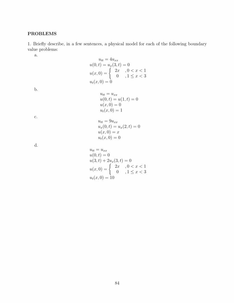
PROBLEMS

1. Briefly describe, in a few sentences, a physical model for each of the following boundaryvalue problems:

a.utt = 4uxx

u(0, t) = ux(3, t) = 0

u(x, 0) =

{2x , 0 < x < 10 , 1 ≤ x < 3

ut(x, 0) = 0

b.utt = uxx

u(0, t) = u(1, t) = 0u(x, 0) = 0ut(x, 0) = 1

c.utt = 9uxx

ux(0, t) = ux(2, t) = 0u(x, 0) = xut(x, 0) = 0

d.utt = uxx

u(0, t) = 0u(3, t) + 2ux(3, t) = 0

u(x, 0) =

{2x , 0 < x < 10 , 1 ≤ x < 3

ut(x, 0) = 10

84

3.6 The Fixed End Condition String

As our first special case, we shall start with the one which is physically the most common.This, as we discussed earlier, occurs when the ends of the string are rigidly attached tosome immovable object - i.e. the fixed end, or Dirichlet boundary conditions. In terms ofthe homogeneous problem (3.5.11) this coincides to α1 = α2 = 1, and β1 = β2 = 0, or u(x, t)satisfies:

utt = c2uxx

u(0, t) = 0u(L, t) = 0u(x, 0) = f(x)ut(x, 0) = g(x)

(3.6.12)

Now, let’s start by reflecting again on our experience with second order, linear ordinarydifferential equations. The first step in these problems was to identify all of the linearlyindependent homogeneous solutions. In the case of constant coefficient equations, this iden-tification was accomplished primarily by assuming a certain solution form (y = erx), thensubstituting that form into the equation, and finally determining the specific values of rfor which non-trivial solutions exist. Once the necessary number of linearly independentsolutions corresponding to these values of r had been constructed, then the general solutionwas formed by taking a linear combination of all the linearly independent solutions i.e. bymultiplying each linearly independent solution by an arbitrary constant and then summingthem together. At this point the initial conditions were considered, in order to determinethe values of the constants in the solution. We will try a somewhat analogous approach here.

If we are then to try a similar procedure here, our first step should be to identify whatconstitutes the homogenous problem in the case of partial differential equations. Consideringthe fixed-end problem (3.5.11), and recalling that in solving for the linearly independenthomogenous solutions in ordinary differential equations, the initial conditions do not enteruntil the very end of the problem, then, according to our normal concept of homogenous,the homogeneous problem without initial conditions for (3.6.12) appears to be

utt = c2uxx

u(0, t) = 0,u(L, t) = 0

(3.6.13)

This problem clearly has at least the trivial solution, u(x, t) = 0. (As does any linearhomogeneous problem! After all, y ≡ 0 solved ay′′ + by′ + cy = 0.) But trivial solutionsare inherently uninteresting. The important question is does (3.6.13) have any non-trivialsolutions? And, if so, how do we find them? And how many of them are linearly independent?(After all, any non-trivial solutions can only be determined up to an arbitrary multiplicativeconstant anyway.)

But wait! Observe that the homogeneous partial differential equation in (3.6.13) possessesa natural “splitting,” in that the left-hand side involves only an operation on the timebehavior of u(x, t) and the right-hand side involves only an operation on the spatial behaviorof u(x, t). This suggests its solutions might also have a splitting of the time behavior from

85

the spatial behavior. (Although this is by no means guaranteed!) So we shall first look forsolutions which have the form:

u(x, t) = X(x)T (t) . (3.6.14)

(This is commonly called the Separation of Variables assumption.) It’s important at thispoint to emphasize that this form is only an assumed solution, just as y = erx was an assumedsolution to py′′ + qy′ + ry = 0. There is of course no guarantee that any of the homogeneoussolutions to the partial differential equation need to be this product form, and certainly noa priori assurance that all of them will be. (For example, not all of the solutions to y′′ +2y′ + y = 0 are “pure” exponentials.) There is only one way to tell whether or not (3.6.14)will really yield valid non-trivial solutions, and that is to substitute it into (3.6.13) and seewhat follows. That is precisely what we shall do next.

In order to substitute (3.6.14) into (3.6.13), we first need to compute the various indicatedderivatives. But, by the basic rules for partial differentiation:

∂2u

∂t2=

∂2

∂t2[X(x)T (t)] = X(x)T ′′(t) ,

and,∂2u

∂x2=

∂2

∂x2[X(x)T (t)] = X ′′(x)T (t) .

Thus, upon substitution, the partial differential equation in (3.6.13) becomes:

X(x)T ′′(t) = c2X ′′(x)T (t) ,

or, dividing both sides by the product c2XT ,

T ′′(t)c2T (t)

=X ′′(x)X(x)

. (3.6.15)

But consider the implication of this last equation carefully. The left-hand side containsonly terms which depend on time, hence it is completely independent of x. The right-handside contains only terms in x, and so is independent of time. But both sides are equal. Thus,each side of this equation is independent of both time and x, and therefore each side mustjust be constant.

We now denote this constant by −λ. (We shall see in a moment there was an ulteriormotive, involving essentially facts which we have not yet developed here, for including theexplicit minus sign. There is really no basis in the information we have developed up to thistime to expect one algebraic sign over of another.) Thus, the equation becomes:

T ′′(t)c2T (t)

=X ′′(x)X(x)

= −λ ,

orT ′′(t) + λc2T (t) = 0 ,X ′′(x) + λX(x) = 0 .

(3.6.16)

86

You should appreciate that at this point there will not necessarily be only a single valueof λ for which this approach works. (After all, there are generally two values of r in thesecond-order ordinary differential equation.) For now, any value for λ should seem as goodas any other. (Actually, this is a slight overstatement. From physical arguments, it seemsunlikely that λ in (3.6.16) could be negative, since then the general solution to the equationfor T(t) would include a growing exponential in time, and such a solution is not physicallyreasonable for normal guitar strings. But mathematically, we cannot yet discard any possiblevalues for λ.)

Actually, the fact that we can’t say anything yet about the value(s) of λ should not bereally surprising, since we have not utilized all the information contained in the homogeneousproblem (3.6.13). Specifically, we have not yet used the boundary conditions. But if ourproduct solution (3.6.14) is to satisfy the entire homogenous problem, it must, of necessity,satisfy not only the partial differential equation, but the boundary conditions in (3.6.13) aswell. So, we substitute the product (3.6.14) into the first (left-hand end) condition, yielding

u(0, t) = X(0)T (t) = 0 . (3.6.17)

But observe that X(0), being the value of a function at one point, is just a number, i.e.a constant. But the product in (3.6.17) is identically zero. Therefore, unless X(0) = 0,then T (t) must be identically zero. But if T (t) were identically zero, then u(x, t) = X(x)T (t)would also be identically zero (trivial), and therefore of no interest to us - we already knowthe trivial solution satisfies the homogeneous problem. What we care about is non-trivialsolutions! Thus, to retain any hope of finding non-trivial solutions, we must require that

X(0) = 0 .

Similarly, at x = L, by an essentially identical argument, we must also have:

u(L, t) = X(L)T (t) = 0⇒ X(L) = 0 .

Now, if we collect all the information we have so far deduced about X(x) and T (t) asdefined by (3.6.14) , we have:

T ′′ + λc2T = 0 X ′′ +λX = 0X(0) = 0X(L) = 0 .

(3.6.18)

Observe the equation for T (t) still has a solution for any value of λ, since there are noconditions on T (t) other than the differential equation. But the same is clearly no longertrue for X(x). After all, the equation for X(x)

X ′′ +λX = 0X(0) = 0X(L) = 0 .

(3.6.19)

is homogeneous and now has two homogeneous boundary conditions. If these were initialconditions, they would be enough to guarantee an unique solution for X(x), which clearly

87

would have to be X(x) ≡ 0. So can we find any λ for which there are non-trivial solutionsas well?

Well, suppose for the moment we can and consider the situation if λ is negative. We canconveniently represent this by writing

λ = −ζ2 ,

where ζ is some non-zero real number. With this substitution, X(x) satisfies:

X ′′ − ζ2X = 0 ,

the general solution to which is

X(x) = c1eζx + c2e

−ζx .

But now we have to determine the constants c1 and c2 so that the boundary conditions aresatisfied. When we do this at x = 0, we have

X(0) = c1 + c2 = 0 =⇒ c2 = −c1 =⇒ X(x) = c1(eζx − e−ζx

).

Then the condition at x = L becomes,

X(L) = c1(eζL − e−ζL

)= 0 .

However, it is easily shown that(eζL − e−ζL

)cannot be zero if L > 0 and ζ = 0. Therefore

we must have c1 = 0, which meansX(x) ≡ 0 ,

or we have only the trivial solution to

X ′′ + λX = 0X(0) = X(L) = 0

when λ < 0. (In view of our earlier comment about not wanting a growing exponential inthe solutions for T (t), this is somewhat of a relief, in that the mathematics confirms ourphysical intuition - a key attribute if we are to consider the model to be valid.) Since we arenot interested in trivial solutions, we drop λ < 0 from any further mention for this problem.

Well, if λ is not negative, then maybe λ is zero. But, in this case, the differential equationfor X(x) becomes

X ′′ = 0 ,

and the general solution to this is

X(x) = d1 + d2x .

Now, we again try to satisfy the boundary conditions with this solution. When x = 0, wehave

X(0) = d1 = 0 =⇒ X(x) = d2x ,

88

and then when x = L,X(L) = d2L = 0 .

Now it is easily seen that the only possible way this can happen is if d2 = 0 and again we haveonly the trivial solution. So λ = 0 must also be discarded for this problem. (We would notethat this should have been clear geometrically, since the differential equation and boundaryconditions for λ = 0 imply that X(x) is a straight line passing through the x-axis at x = 0and x = L, and X(x) ≡ 0 is obviously the only solution to these conditions!)

We are now about at the end of our rope. Our only remaining hope of finding non-trivialsolutions in the form (3.6.14) rests with the possibility that λ is positive. In this case, wecould write,

λ = ξ2

where ξ is some non-zero real number. Then X(x) would satisfy the differential equation

X ′′ + ξ2X = 0 ,

whose general solution isX(x) = a1 sin(ξx) + a2 cos(ξx) .

Again we must try to pick a1 and a2 so that the boundary conditions are satisfied. Thisyields first, at x = 0

X(0) = a2 = 0 =⇒ X(x) = a1 sin(ξx) ,

and then, at x = L,X(L) = a1 sin(ξL) = 0 . (3.6.20)

But now there is a major difference between this equation and the cases when λ < 0 or λ = 0!Neither of the two terms in (3.6.20) are automatically non-zero. We could in fact stillset a1 = 0, and get the trivial solution, but this is no longer necessary in order to satisfythe boundary condition! We could equally well arrange for sin(ξL) to be zero, simply bypicking ξL to be an integer multiple of π. In this latter case, the a1 could remain non-zero!

But which integer should we use? ξL = π works, but so do ξL = 2π, and ξL = 3π,and ξL = 4π, and so forth. In fact any time we pick

ξL = nπ , n = 1, 2, 3, . . . ,

we get a non-zero value for a1 and hence a non-trivial solution. For the sake of convenience,we shall denote these different values with a subscript, as

ξn =nπ

L, n = 1, 2, 3, . . . . (3.6.21)

Thus, for each different value of ξn, we get another non-trivial solution to:

X ′′ + ξ2X = 0 ,X(0) = X(L) = 0 ,

89

and we shall denote that solution by:

Xn(x) = sin(ξnx) = sin(nπx

L

), n = 1, 2, 3, . . . . (3.6.22)

Note we have dropped the arbitrary constant in the solution X(x). We did this since wehave already observed that, as solutions to a linear, homogeneous problem, the X(x) canonly be determined up to an arbitrary constant anyway. So we are only interested in thelinearly independent solutions to this problem! Interestingly, we have passed, in one step,from having doubts about whether or not the splitting we assumed in (3.6.14) would workfor any λ, to the determination that it works for an infinite number of different values of λ,given by

λn =(nπ

L

)2

, n = 1, 2, 3, . . . . (3.6.23)

Returning to the equation for T (t), we see that for each value of λn given by (3.6.23),there are two linearly independent solutions, which we can represent as

Tn(t) = An cos(nπct

L

)+Bn sin

(nπct

L

), n = 1, 2, 3, . . . .

Finally, combining the various pieces, we see that for each value of λ given by (3.6.23),theseparation of variables form (3.6.14) produces two non-trivial, linearly independent solutionsto (3.6.13) given by:

un(x, t) = Xn(x)Tn(t)

=[An cos

(nπct

L

)+Bn sin

(nπct

L

)]sin

(nπx

L

), n = 1, 2, 3, . . . .

(3.6.24)

(At this point, we shall pause momentarily to reflect on what has just happened. We had alinear, homogeneous problem, given by (3.6.13), and containing a parameter, λ. This typeof problem normally would have only the trivial solution. Upon substitution, however, wefound that non-trivial solutions did in fact exist, but only for certain specified values of theparameter. This behavior is qualitatively similar to that encountered in the study of systemsof linear algebraic equations with the matrix-vector equation

Ax = λx ,

where x is an n-dimensional vector, and A is a constant matrix. This equation has non-trivialsolutions if and only if λ satisfies

det(A− λI) = 0 ,

that is, if λ is an eigenvalue of A and x the corresponding eigenvector. Because of thesesimilarities, we call the λ as given by (3.6.23) the eigenvalues of the problem (3.6.19). Ina similar vein the non-trivial solutions Xn(x) given by (3.6.22) are often referred to as theeigenfunctions.)

90

We now proceed. With (3.6.24) we seem to have identified all the linearly independentsolutions to (3.6.13). (Although we have not proven this, their number would indicate it.)Therefore, since the basic problem was linear, we should be able to form the general solutionby taking an arbitrary linear combination of the linearly independent homogeneous solutions,just as the general solution to

y′′ + 2y′ + y = 0

is given as a linear combination of e−x and xe−x, i.e. as y(x) = c1e−x + c2xe

−x .Following this logic, the general solution to (3.6.13) should be given by

u(x, t) =[A1 cos

(πct

L

)+B1 sin

(πct

L

)]sin

(πx

L

)+

[A2 cos

(2πct

L

)+B2 sin

(2πct

L

)]sin

(2πx

L

)+

[A3 cos

(3πct

L

)+B3 sin

(3πct

L

)]sin

(3πx

L

)+ · · · ,

(3.6.25)

where the Ai and Bi, i = 1, 2, 3, . . . are arbitrary constants.Note that we can save a great deal of writing by using instead the shorthand

u(x, t) =∞∑

n=1

[An cos

(nπct

L

)+Bn sin

(nπct

L

)]sin

(nπx

L

). (3.6.26)

But, if this really represents the general solution to (3.6.13) , then it must be able, for aproper choice of the constants Ai and Bi, to satisfy any initial conditions we would wish toapply, and specifically to satisfy the initial conditions given in (3.6.13),

u(x, 0) = f(x) ,ut(x, 0) = g(x) .

Can this, in fact satisfy the conditions? There is really but one way to find out, and that isto take our “general solution” and substitute it into these equations. Therefore we let t = 0in (3.6.26), which is supposed to represent u(x, t) at all times and substitute that expressionfor u(x, 0) in the initial conditions. This produces

f(x) = u(x, 0) =∞∑

n=1

An sin(nπx

L

). (3.6.27)

Now can we find the An so that this is satisfied? The answer, of course, is yes, provided f(x)is at least piecewise smooth on 0 < x < L. Physically, this must almost certainly bethe case, since it is difficult to conceive of any guitar string in the “real world” whosedisplacements are not at least piecewise smooth. (Really, it’s quite difficult to think of anythat are not continuous!) So all we need do is extend f(x) oddly into the region −L < x < 0.Since (3.6.27) is nothing more than the Fourier sine series for this extension, its coefficients(the An) are given by:

An =2

L

∫ L

0f(x) sin

(nπx

L

)dx . (3.6.28)

91

For the second initial condition, we must first differentiate (3.6.26) to obtain an expressionfor ut(x, t),

ut(x, t) =∞∑

n=1

[−nπc

LAn sin

(nπct

L

)+nπc

LBn cos

(nπct

L

)]sin

(nπx

L

),

and then let t = 0 and substitute into the second initial condition, to get

ut(x, 0) =∞∑

n=1

nπc

LBn sin

(nπx

L

). (3.6.29)

But this is simply another Fourier sine series, except with an effective coefficient of nπcLBn

instead of bn. Therefore, by the usual rule for computing these coefficients, we simplyimagine g(x) to be oddly extended and then

nπc

LBn =

2

L

∫ L

0g(x) sin

(nπx

L

)dx ,

or

Bn =2

nπc

∫ L

0g(x) sin

(nπx

L

)dx . (3.6.30)

This clearly indicates that the Bn can also be computed provided the initial velocity, g(x) isat least piecewise smooth - which from physical considerations it really needs to be.

Therefore, we see that we can satisfy any initial condition for the homogeneous partialdifferential equation (3.6.13) with the solution form (3.6.26), and hence we seem to have infact found the general solution.

But wait a minute! The solution as defined by (3.6.26) involves an infinite series, and someinfinite series are known not to converge. Is it possible that we might find in some problemsthat the solution did not converge? Fortunately, here, the answer is no! This is becauseit is easily shown that, since sin(nπct/L) and cos(nπct/L) are always less than or equal toone in magnitude, then (3.6.26) will always converge provided the original Fourier sine series(3.6.27) did. But, the original Fourier sine is known to converge from the basic principles ofFourier series (provided the initial displacement and velocity are piecewise smooth), so thereis no problem.

As an example, consider the problem

utt = uxx , 0 < x < 2 , 0 < t ,u(0, t) = 0 ,u(2, t) = 0 ,

u(x, 0) ={x , 0 < x ≤ 12− x , 1 < x < 2

ut(x, 0) = 0

This problem describes the an elastic string of length two, fixed at both ends, which wasdisplaced by lifting up at the center to the shape shown in Figure 29, held there, and thenat t = 0 released. (At the instant of release, its velocity is thus zero, even though itsacceleration is not.)

92

u

x

2

1

Figure 29: The Initial Displacement - u(x, 0)

If we retrace the steps from (3.6.13) on for this problem, we see that the eigenfunctionssatisfy

X ′′ + λX = 0 ,X(0) = X(2) = 0 ,

and are therefore

Xn(x) = sin(nπx

2

), n = 1, 2, 3, . . . .

The eigenvalues are

λn = ξ2n =

(nπ

2

)2

, n = 1, 2, 3, . . .

Thus, the general solution to this problem looks like

u(x, t) =∞∑

n=1

[An cos

(nπt

2

)+Bn sin

(nπt

2

)]sin

(nπx

2

).

The initial displacement becomes,

u(x, 0) =∞∑

n=1

An sin(nπx

2

)={

x , 0 ≤ x ≤ 12− x , 1 < x ≤ 2

,

and, therefore, by the usual Fourier formulas

An = 22

∫ 2

0f(x) sin

(nπx

2

)dx

=∫ 1

0x sin

(nπx

2

)dx+

∫ 2

1(2− x) sin

(nπx

2

)dx

=

{− 2

nπx cos

(nπx

2

)+[

2

nπ

]2

sin(nπx

2

)}∣∣∣∣∣1

0

+

{− 2

nπ(2− x) cos

(nπx

2

)−[

2

nπ

]2

sin(nπx

2

)}∣∣∣∣∣2

1

= 2[

2

nπ

]2

sin(nπ

2

).

93

Similarly, the initial condition on the velocity, ut(x, 0), yields

Bn = 0 ,

and therefore,

u(x, t) =∞∑

n=1

2[

2

nπ

]2

sin(nπ

2

)cos

(nπt

2

)sin

(nπx

2

).

94

PROBLEMS

1. Solve:utt = uxx

u(0, t) = u(3, t) = 0

u(x, 0) =

⎧⎪⎨⎪⎩

2x , 0 < x < 1/22− 2x , 1/2 ≤ x < 1

0 , 1 ≤ x < 3ut(x, 0) = 0

Sketch the ten-term partial sum of your computed solution at

t = 0, 1, 2, 4 .

2. Solve:utt = uxx

u(0, t) = u(π, t) = 0

u(x, 0) =

⎧⎪⎪⎪⎨⎪⎪⎪⎩

0 , 0 < x < π/4(4x− π)/π , π/4 ≤ x ≤ π/2(3π − 4x)/π , π/2 ≤ x ≤ 3π/4

0 , 3π/4 < x < πut(x, 0) = 0

3. Solve:utt = uxx

u(0, t) = u(π, t) = 0u(x, 0) = x(π − x), 0 < x < πut(x, 0) = 0

4. Solve:utt = uxx

u(0, t) = u(3, t) = 0u(x, 0) = 0ut(x, 0) = x

5. Solve:utt = 9uxx

u(0, t) = u(π, t) = 0u(x, 0) = sin(x)ut(x, 0) = 1

6. Solve:utt = 4uxx

u(0, t) = u(5, t) = 0

ut(x, 0) =

{x , 0 < x < 5/2

5− x , 5/2 ≤ x < 5u(x, 0) = 0

95

7. The dissipation of heat in a “very large” solid slab of thickness L whose faces are held ata fixed reference temperature of 0o is described by the partial differential equation:

ut = kuxx

u(0, t) = u(L, t) = 0u(x, 0) = f(x)

where u(x, t) denotes the temperature at location x and time t.a. Why is only one initial condition required in this problem?b. Show that the method of Separation of Variables also “works” in this problem, and

leads formally to the general solution:

u(x, t) =∞∑

n=1

bne−k(nπ/L)2t sin

(nπx

L

),

where:

bn =2

L

∫ L

0f(x) sin

(nπx

L

)dx .

96

3.7 The Free End Conditions Problem

As we have already indicated, our general approach to the study of the one-dimensional waveequation (3.5.11) was to first solve several special cases, and then try to deduce the main as-pects of the general theory from these specific cases. Each case would correspond to differentspecific boundary conditions (i.e. values of α and β in (3.5.11)). In the previous section, ourfirst case, we developed the solutions to the fixed end condition (Dirichlet) problem. Therewe saw that the separation of variables assumption, applied to the homogeneous problemwithout initial conditions, leads to an infinite number of linearly independent solutions deter-mined by the eigenvalues of the problem. Furthermore, after we formed the general solutionas a linear combination of these solutions, we found that satisfying the initial conditionsreduced to nothing more than an ordinary Fourier sine series. The obvious question whichwe must now pursue is how much of this behavior will any one-dimensional wave equationshare, and which aspects were purely example (Dirichlet boundary conditions) specific? Toanswer this, we must of course study more cases.

In this section, we consider a second special case, specifically that of α1 = α2 = 0,and β1 = β2 = 1, or u(x, t) satisfying:

utt = c2uxx

ux(0, t) = 0ux(L, t) = 0u(x, 0) = f(x)ut(x, 0) = g(x)

(3.7.31)

Physically, this problem could represent a string with frictionless slip rings located at bothends (Figure 30). Mathematically, as mentioned during the derivation of the various bound-ary conditions, we call this problem the free end condition problem, or, alternatively, say ithas Neumann conditions at both ends. (Before reading further, you should pause to reflect,physically, on what qualitative properties you might expect a solutions to this problem wouldhave.)

We will, of course, want to apply to this problem, as much as possible, our experiencewith the Dirichlet conditions. (After all, there is very little profit in “reinventing the wheel,”or in repeating mathematical steps when you know (or should know) ahead of time whatthe result will be.) Since, in the Dirichlet case, we started with the homogeneous problemwithout initial conditions, if we were to proceed similarly with (3.7.31), then we should startwith

utt = c2 uxx

ux(0, t) = 0,ux(L, t) = 0

(3.7.32)

Clearly, as also occurred with the Dirichlet case, this problem always has at least the trivialsolution, and again the important question becomes what are its linearly independent non-trivial solutions, and how do we find them?

Well, observe that the partial differential equation in (3.7.32) has not changed from theDirichlet problem, and so still possesses the same natural splitting of the time and spatialoperations. Therefore it seems quite reasonable to use the same separation of variables

97

Figure 30: The Free End Conditions Problem

form (3.6.14) here. Moreover, since the partial differential equation is unchanged (only theboundary conditions have changed), substituting the product form into the partial differentialequation must produce exactly the same separated ordinary differential equations, i.e.

T ′′(t) + λc2T (t) = 0 X ′′(x) + λX(x) = 0 .

Keep in mind that at this point λ does not necessarily represent any single value. In fact,based on our last example we should almost certainly expect an infinite number of differentvalues will “work” here also. But what are they? After all, the boundary conditions aren’tthe same as in the last case, so there’s no reason to expect the same solutions. It stilldoes seem unlikely from physical arguments that λ could be negative, since exponentiallygrowing solutions (T (t)) seem no more physically reasonable here than they were before. But,mathematically, we can’t assume anything yet about possible values for λ for this problem.

This last point shouldn’t really be surprising, since, of course, we haven’t yet consideredthe boundary conditions for this problem, and the boundary conditions were crucial indetermining the eigenvalues of the fixed end problem. Furthermore, since the boundaryconditions for this problem (3.7.31) are not the same as in the Dirichlet case, we can’tsay X(0) = X(L) = 0, but must derive a new set of conditions, appropriate for this case,by substituting the separation of variables form (3.6.14) directly into boundary conditionsin (3.7.32). That substitution yields

ux(0, t) = X ′(0)T (t) = 0 ,

which, since X ′(0) must just be a constant, requires,

X ′(0) = 0 .

98

if we are to have non-trivial solutions. An essentially identical argument at x = L leads to

ux(L, t) = X ′(L)T (t) = 0⇒ X ′(L) = 0 .

Thus, with our new set of boundary conditions, we now have the complete set of separatedequations

T ′′ + λc2T = 0 X ′′ +λX = 0X ′(0) = 0X ′(L) = 0 .

(3.7.33)

Observe that in these equations, as in the fixed end case, the equation for T (t) is solvablefor any value of λ. This still seems reasonable since we have not yet applied any initialconditions. Furthermore, the equation for X(x)

X ′′ +λX = 0X ′(0) = 0X ′(L) = 0 .

(3.7.34)

is again homogeneous with homogenous boundary conditions, and so clearly still has thetrivial solution. Therefore, the fundamental question we must answer has not changed fromthe Dirichlet problem - for what values of λ are there non-trivial solutions to (3.7.34)? Well,unless we’re clairvoyant, there’s no way to answer this other than to basically repeat thesame procedure as before, i.e. assuming, in sequence, negative, zero and positive valuesfor λ, and seeing if these produce any solutions.

As before, we start by assuming λ could be negative, and again represent this by

λ = −ζ2 , ζ = 0 .

This yieldsX(x) = c1e

ζx + c2e−ζx ,

and therefore the boundary conditions reduce to

X ′(0) = ζc1 − ζc2 = 0X ′(L) = ζc1e

ζL − ζc2e−ζL = 0 ,

which since ζ and L are non-zero, can be shown to be satisfied only by c1 = c2 = 0. Thus,as before, we have only the trivial solution when λ < 0 (which again coincides with ourearlier expectation that growing exponentials still should not occur in the solutions for T (t).)So λ < 0 may be dropped from further consideration for this problem.

Next, we must check whether λ can be zero. Well, if this is the case, then

X(x) = d1 + d2x ,

and when we substitute this solution into the free boundary conditions, we find

X ′(0) = d2 = 0X ′(L) = d2 = 0 .

99

But wait! This requires that d2 = 0, but it doesn’t say anything about d1, which apparentlycan have any value. Therefore here, unlike the fixed end case, λ = 0 does not produce onlythe trivial solution, and so cannot be dropped in this problem. In fact, according to ourdefinitions, zero is clearly an eigenvalue here. The corresponding eigenfunction is a constant,which, since we are only interested in linearly independent solutions, we can assign to be anyconvenient value. For purposes which should become clear later, we now chose this value tobe 1

2. Thus, in summary, we have

λ0 = 0X0(x) = 1

2

(You might note again that this conclusion should have been obvious from a geometricalinterpretation of the λ = 0 condition, which only requires a straight line parallel to thex-axis at x = 0 and x = L.)

But, of course, so far we really have only half the answer at λ = 0! Our real goal isto identify the linearly independent solutions u(x, t). Therefore each X(x) must have acorresponding T (t). When λ0 = 0, T (t) must clearly satisfy the differential equation

T ′′0 = 0⇒ T0(t) = A0 +B0t ,

and therefore the corresponding product solution becomes

u0(x, t) = X0(x)T0(t) = 12[A0 +B0t] .

But we can’t stop yet! We have to identify all of the linearly independent homogeneoussolutions, and the fixed end problem had an infinite number of different eigenvalues. So itdoesn’t seem reasonable that this problem would have only one! Therefore, we must alsoinvestigate whether any non-trivial solutions exist for λ positive. Thus we write,

λ = ξ2

where ξ is some non-zero real number. This gives the as general solution for (3.7.34)

X(x) = a1 sin(ξx) + a2 cos(ξx) ,

and again we must try to pick a1 and a2, not both zero, so that the boundary conditions aresatisfied. For the free boundary conditions, this leads, at x = 0, to

X ′(0) = a1ξ = 0⇒ X(x) = a2 cos(ξx)

(since ξ was assumed non-zero). Then, at x = L, the boundary condition reduces to

X ′(L) = −a2ξ sin(ξL) = 0 , ξ = 0 .

Here, as in the fixed end case, and unlike the situation when λ is negative, it’s not necessaryto set the a2 equal to zero (and so have only the trivial solution) in order to satisfy the

100

boundary condition! We could again keep a2 non-zero by making sin(ξL) zero, using thesame eigenvalues as worked before, i.e.

ξn =nπ

L,

λn =(nπ

L

)2

,

n = 1, 2, 3, . . . . (3.7.35)

But there is an important difference here compared to the fixed-end case - even though theeigenvalues have not changed, a review of these last steps shows that the eigenfunctionshave. In fact, the eigenfunctions here are

Xn(x) = cos(ξnx) = cos(nπx

L

), n = 1, 2, 3, . . . (3.7.36)

(where we have again dropped the arbitrary constant since we only care about linearlyindependent solutions). Geometrically these eigenfunctions reflect the fact that, for λ > 0,equation (3.7.34) may be viewed as simply specifying those sinusoidal functions with zeroslope at both ends of the interval!

As before, each eigenvalue given by (3.7.35) also determines a corresponding differentialequation for the T (t), whose solution involves two linearly independent solutions which canbe represented as

Tn(t) = An cos(nπct

L

)+Bn sin

(nπct

L

), n = 1, 2, 3, . . . .

Combining all of this information, we see that each positive eigenvalue produces two non-trivial, linearly independent solutions to (3.7.32) given by:

un(x, t) = Xn(x)Tn(t)

=[An cos

(nπct

L

)+Bn sin

(nπct

L

)]cos

(nπx

L

), n = 1, 2, 3, . . . .

(3.7.37)

By this point, we would again seem to have identified all the linearly independent solu-tions to (3.7.32). (Although again we have not proven this.) Therefore, we now form thegeneral solution by taking an arbitrary linear combination of all the linearly independenthomogeneous solutions (including λ = 0), to yield

u(x, t) = 12[A0 +B0t] +

[A1 cos

(πct

L

)+B1 sin

(πct

L

)]cos

(πx

L

)+

[A2 cos

(2πct

L

)+B2 sin

(2πct

L

)]cos

(2πx

L

)+

[A3 cos

(3πct

L

)+B3 sin

(3πct

L

)]cos

(3πx

L

)+ · · · ,

= 12[A0 +B0t] +

∞∑n=1

[An cos

(nπct

L

)+Bn sin

(nπct

L

)]cos

(nπx

L

),

(3.7.38)

101

where the Ai and Bi, i = 0, 1, 2, . . . still have to be determined. Moreover, as before, if thisreally represents the general solution to (3.7.32), then we have to be able to determine theconstants Ai and Bi so as to satisfy any set of initial conditions we would wish to apply, andspecifically for the initial conditions

u(x, 0) = f(x) ,ut(x, 0) = g(x) .

To see whether we can accomplish this here, we must, as we did before, substitute (3.7.38),which is supposed to represent u(x, t) at all times, directly into the expressions for u(x, 0)and ut(x, 0). If we do this, we have,

u(x, 0) = f(x) = 12A0 +

∞∑n=1

An cos(nπx

L

), 0 < x < L ,

and

ut(x, 0) = g(x) = 12B0 +

∞∑n=1

nπc

LBn cos

(nπx

L

), 0 < x < L .

(3.7.39)

Now can we find the An and Bn that satisfy these? The answer, as in the fixed endcase, is yes, provided f(x) and g(x) are at least piecewise smooth on 0 < x < L (Which,from physical considerations, should clearly be the case). There is, however, one change. Inthis problem we must use even extensions, rather than odd ones, since only even functionhave Fourier cosine series (which are all (3.7.39) represent). Computing these coefficients inthe usual way (recognizing that the effective coefficient in the second series is nπc

LBn instead

of an) yields

An =2

L

∫ L

0f(x) cos

(nπx

L

)dx , n = 0, 1, 2, . . .

B0 =2

L

∫ L

0g(x)dx ,

Bn =2

nπc

∫ L

0g(x) cos

(nπx

L

)dx , n = 1, 2, 3, . . . .

(3.7.40)

Therefore, we have found that solution form (3.7.38) can satisfy any initial condition forthe homogeneous partial differential equation (3.7.31), and hence does in fact represent thegeneral solution. (Mathematically, as in the case of the series solution to the fixed endcase, (3.7.38) really only represents only a formal solution. That is, it’s not valid unless theinfinite series involved converge. Fortunately though, here as before, we could show that thisseries will always converge provided the initial condition Fourier cosine series (3.7.39) did.)

We cannot leave this problem, however, without pointing out one additional intriguingfeature of (3.7.38) that we did not see in the Dirichlet solution - the presence of the 1

2[A0+B0t]

term. What does this represent? What would be the meaning of

12A0 =

1

L

∫ L

0f(x)dx = 0 ?

102

And how should we interpret

12B0 =

1

L

∫ L

0g(x)dx = 0 ?

(We will leave the reader to reflect on these questions!)To illustrate this general class of problems, consider the example

utt = uxx , 0 < x < 4 , 0 < t ,ux(0, t) = 0 ,ux(4, t) = 0 ,

u(x, 0) =

⎧⎪⎪⎪⎨⎪⎪⎪⎩

0 , 0 < x ≤ 1x− 1 , 1 < x < 23− x , 2 ≤ x ≤ 3

0 , 3 < x < 4ut(x, 0) = 0

This problem describes an elastic string of length four, free at both ends, whose middle halfis displaced into a triangular shape, held there, and then released at t = 0. (See Figure 31.)Note that c = 1 for this example.

x

40

1

Figure 31: The Initial Displacement f(x)

If we retrace the steps from (3.7.32) on for this problem, we see that the eigenfunctionssatisfy

X ′′ + λX = 0 ,X ′(0) = X ′(4) = 0 ,

and therefore the eigenvalues are

λ0 = 0 and λn =nπx

4, n = 1, 2, 3, . . . ,

with corresponding eigenfunctions

X0(x) = 12

and Xn(x) = cos(nπx

4

), n = 1, 2, 3, . . . ,

respectively. Thus, according to the steps outlined in this chapter, the general solution tothis problem is

u(x, t) = 12[A0 +B0t] +

∞∑n=1

[An cos

(nπt

4

)+Bn sin

(nπt

4

)]cos

(nπx

4

).

103

The initial conditions become,

u(x, 0) = 12A0 +

∞∑n=1

An cos(nπx

4

)=

⎧⎪⎪⎪⎨⎪⎪⎪⎩

0 , 0 < x ≤ 1x− 1 , 1 < x < 23− x , 2 ≤ x ≤ 3

0 , 3 < x < 4

and,

ut(x, 0) = g(x) = 12B0 +

∞∑n=1

nπ

LBn cos

(nπx

4

)= 0 .

Therefore, by the usual Fourier formulas

12A0 = 1

4

An = 24

∫ 4

0f(x) cos

(nπx

4

)dx

= 12

∫ 2

1(x− 1) cos

(nπx

4

)dx+ 1

2

∫ 3

2(3− x) cos

(nπx

4

)dx

=1

2

[4

nπ

]2 [2 cos

(nπ

2

)− cos

(nπ

4

)− cos

(3nπ

4

)]

Bn ≡ 0 , n = 0, 1, 2, . . . .

Note the value of1

2A0 here - it’s simply the average height, along the string, of the initial

displacement, i.e. the center of mass in the vertical direction of the string. Furthermore,there are no external forces acting on this string, and the average value of cos

(nπt4

)is zero!

This implies that since Bn ≡ 0, we could view this solution as a vibration about a fixed,offset center of mass. (If you’re still not sure how to interpret the B0 in the general case, tryapplying conservation of momentum to the initial conditions in (3.7.31).)

104

PROBLEMS

1. Solve:utt = 25uxx

ux(0, t) = ux(1, t) = 0

u(x, 0) =

⎧⎪⎨⎪⎩

0 , 0 < x < 1/4x− 1/4 , 1/4 < x < 3/4

1/2 , 3/4 < x < 1ut(x, 0) = 0

Interpret the solution physically.

2. Solve:utt = uxx

ux(0, t) = ux(2, t) = 0

u(x, 0) =

⎧⎪⎨⎪⎩

2x , 0 < x < 1/22− 2x , 1/2 ≤ x ≤ 3/22x− 4 , 3/2 < x < 2

ut(x, 0) = 1

Interpret the solution physically.

105

3.8 The Mixed End Conditions Problem

Thus far, we have solved two special cases of the one-dimensional wave equation in our effortto develop a “feel” for the general behavior of the solutions to this equation. In both ofthese cases, the separation of variables assumption, applied to the homogeneous parts of theproblem, produced an infinite number of linearly independent solutions, as determined by theeigenvalues. These eigenvalues, however, and their associated eigenfunctions, were problemdependent, i.e. they changed with the problem, although in neither case were the eigenvaluesnegative, and in only one of the two cases zero was an eigenvalue. Furthermore, in bothcases, the general solution we formed as a linear combination of these solutions reduced toan ordinary Fourier series when applied to the initial conditions. The fundamental questionstill in front of us is how many of these properties will remain unchanged as we study morecases.

Therefore, we continue by investigating a third case,

utt = c2uxx

u(0, t) = 0ux(L, t) = 0u(x, 0) = f(x)ut(x, 0) = g(x) .

(3.8.41)

(In terms of our standard form (3.5.11), this newest case corresponds to

α1 = β2 = 1 and β1 = α2 = 0 . )

Physically, this equation could model a string fixed at the left end, with a frictionlessslip ring located at the right end (Figure 32). Mathematically, we may either refer to thisas the mixed end condition problem, or say the problem has Dirichlet conditions at the leftand Neumann conditions at the right. In this point, as in any problem, you should pause,before continuing, and consider what qualitative physical and mathematical properties youmight expect to find in the solution.

We will, of course, want to apply here as much as possible of our experience with the twoearlier problems. In both of these examples, we started by considering just the homogeneousparts of the problem (without the initial conditions). So it seems reasonable to start herewith

utt = c2uxx

u(0, t) = 0ux(L, t) = 0

(3.8.42)

Given (3.8.42), the important question, as it was in the two previous cases, is what are thelinearly independent, non-trivial solutions, and how do we find them? The answer in thisnew case is not obvious a priori, but having already solved the earlier cases, we should atleast be able to skip many of the intermediate details.

For example, the partial differential equation has still not changed, and therefore theseparation of variables form (3.6.14) should (and does) produce exactly the same two sepa-rated ordinary differential equations. Furthermore, we have already separated the left-hand

106

Figure 32: The Mixed End Condition Problem

boundary condition in our first example, and the right-hand condition in our second one.Thus, we proceed to immediately write the separated problems

T ′′ + λc2T = 0 X ′′ +λX = 0X(0) = 0X ′(L) = 0 .

(3.8.43)

As before, the equation for T (t) will produce two linearly independent solutions for any valueof λ. (By now, as long as we don’t apply initial conditions, we should expect this behavior.)Therefore, as in the earlier cases, the fundamental question remains the same - for whatvalues of λ does

X ′′ + λX = 0X(0) = 0X ′(L) = 0

(3.8.44)

have non-trivial solutions? The procedure for answering this question also remains the same,i.e. considering, in sequence, negative, zero and positive values for λ, and seeing which ofthese do produce solutions.

In the current example, when λ is negative, and represented by λ = −ζ2 (ζ = 0), wehave as the general solution for X(x)

X(x) = c1eζx + c2e

−ζx ,

and therefore the boundary conditions reduce to

X(0) = c1 + c2 = 0

X ′(L) = ζc1eζL − ζc2e−ζL = 0 ,

107

which again can be shown to be satisfied only by c1 = c2 = 0. So negative values of λstill produce only trivial solutions, and therefore growing exponentials for T (t) are stillmathematically (and physically) impossible.

When λ is zero, the general solution to the ordinary differential equation is still

X(x) = d1 + d2x ,

and, when substituted into the boundary conditions, this yields

X(0) = d1 = 0X ′(L) = d2 = 0

.

So we’re back, in this problem, to only trivial solutions when λ = 0, and therefore zero is notan eigenvalue here. (Geometrically, this conclusion should be intuitive, since the problemfor λ = 0 can be viewed as defining a straight line which passes through the x-axis at x = 0,and is horizontal at x = L.)

Lastly, we must consider whether positive values of λ generate non-trivial solutions. (Thisshould by now seem highly likely, since they have in both previous cases). Following ourusual convention of letting λ = ξ2, where ξ = 0, again gives

X(x) = a1 sin(ξx) + a2 cos(ξx) .

The boundary conditions in this case, however, produce a slightly different result than wehave seen previously when we try to determine the a1 and a2. Specifically,

X(0) = a2 = 0⇒ X(x) = a1 sin(ξx)

and thenX ′(L) = a1ξ cos(ξL) = 0 , ξ = 0 .

Here, as in the fixed and free end examples, the important point is that we don’t haveto choose a1 = 0 and get only the trivial solution. However, in order to avoid the trivialsolution, we do have to change our condition for selecting ξ from sin(ξL) = 0 to

cos(ξL) = 0 .

This new condition, of course, will be true only for

ξL =π

2,

3π

2,

5π

2, . . . ,

or, equivalently

ξn =(2n− 1)π

2L, n = 1, 2, 3, . . . ,

λn =

[(2n− 1)π

2L

]2

, n = 1, 2, 3, . . . .

(3.8.45)

108

This is a deviation, albeit minor, from the earlier cases we studied - the positive eigenvaluesare not the same as in the “pure” fixed end or free end cases. Neither are the eigenfunctions

Xn(x) = sin(ξnx) = sin

((2n− 1)πx

2L

), n = 1, 2, 3, . . . (3.8.46)

(Note we have continued our practice of dropping the arbitrary constant when only onelinearly independent solution exists. Also we use (2n − 1) simply as a convenient way ofgenerating the odd integers. We could have equally correctly written

Xn(x) = sin(nπx

2L

), n = 1, 3, 5, . . . ,

etc. This latter representation, however, is not generally used since it becomes more cum-bersome.)

Now, as before, corresponding to each eigenvalue given by (3.8.45) there are two linearlyindependent solutions for T (t), which can be represented in this case as

Tn(t) = An cos

((2n− 1)πct

2L

)+Bn sin

((2n− 1)πct

2L

), n = 1, 2, 3, . . . ,

and therefore there are also two linearly independent solutions to (3.8.42) given by:

un(x, t) = Xn(x)Tn(t)

=[An cos

((2n−1)πct

2L

)+Bn sin

((2n−1)πct

2L

)]sin

((2n−1)πx

2L

),

n = 1, 2, 3, . . . .

Again, since we should by now have identified all the linearly independent solutions, we formthe general solution in the usual way, as

u(x, t) =[A1 cos

(πct

2L

)+B1 sin

(πct

2L

)]sin

(πx

2L

)+

[A2 cos

(3πct

2L

)+B2 sin

(3πct

2L

)]sin

(3πx

2L

)+

[A3 cos

(5πct

2L

)+B3 sin

(5πct

2L

)]sin

(5πx

2L

)+ · · · ,

=∞∑

n=1

[An cos

((2n− 1)πct

2L

)+Bn sin

((2n− 1)πct

2L

)]sin

((2n− 1)πx

2L

).

(3.8.47)Continuing as before, we attempt to determine the constants Ai and Bi, i = 1, 2, 3, . . . by

109

substituting (3.8.47) into the initial conditions. This yields,

u(x, 0) = f(x) =∞∑

n=1

An sin

((2n− 1)πx

2L

), 0 < x < L ,

and

ut(x, 0) = g(x) =∞∑

n=1

(2n− 1)πc

2LBn sin

((2n− 1)πx

2L

), 0 < x < L .

(3.8.48)

Again, (3.8.48) poses an identical question to that we faced in earlier examples - how do wefind the An and Bn that satisfy these? Unlike the earlier problems we studied, however, theanswer here is not as clear. One difficulty is that the series in (3.8.48), while they are Fouriersine series, have a period of 4L, not 2L. (Look at the denominators carefully.) Therefore,even if f(x) and g(x) are at least piecewise smooth on 0 < x < L, and we extend them oddlyinto −L < x < 0, we don’t have enough values to use the Fourier sine series formulas directly.We’re missing the values of f(x) for into L < x < 2L and −2L < x < −L! (Actually, sincewe’re using sine series, only the values from L < x < 2L really matter.) So what do we donow?

Well, one choice is to still try to use odd and even Fourier series concepts. After all, thegeneral Fourier sine series of period 2L has the form

∞∑n=1

bn sin(nπx

2L

)= b1 sin

(πx

2L

)+b2 sin

(2πx

2L

)+ b3 sin

(3πx

2L

)

+ b4 sin(

4πx

2L

)+ b5 sin

(5πx

2L

)+ · · · .

So then, all (?) we seem need to do in order to satisfy the first of (3.8.48) is figure out howto extend f(x) into the interval L < x < 2L in such a way that

b2 = b4 = · · · = 0 and A1 = b1 , A2 = b3 , A3 = b5 , . . . .

We could actually do this, but, as things turn out, such an approach simply delays theinevitable!

The better way to find the coefficients in (3.8.48) is to return to fundamental principles,and ask why was it so important in our earlier examples that the initial conditions reduceto elementary Fourier series? The straightforward answer would seem to be because wecould then immediately compute the coefficients. But that’s too superficial. Why could wecompute the coefficients? The answer is because the orthogonality of the sines and cosines,i.e. the integrals like

∫ 2L

−2Lsin

(nπx

2L

)sin

(mπx

2L

)dx = 0 , m = n ,

allowed use to derive the appropriate formulas. Therefore, before we try various, perhapsartificial, extensions in (3.8.48), we should ask instead if perhaps the functions in those series,

110

i.e. the eigenfunctions, are themselves also orthogonal on the interval 0 < x < L. This meansconsidering the integral

∫ L

0sin

((2n− 1)πx

2L

)sin

((2m− 1)πx

2L

)dx .

Using standard trigonometric identities we have

∫ L

0sin

((2n− 1)πx

2L

)sin

((2m− 1)πx

2L

)dx

=1

2

{∫ L

0cos

(((2n− 1)− (2m− 1))πx

2L

)dx

+∫ L

0cos

(((2n− 1) + (2m− 1))πx

2L

)dx

}

=1

2

{∫ L

0cos

((n−m)πx

L

)dx+

∫ L

0cos

((m+ n− 1)πx

L

)dx

}

=

⎧⎪⎪⎪⎪⎨⎪⎪⎪⎪⎩

12

{L

(n−m)πsin

((n−m)πx

L

)∣∣∣L0

+ L(m+n−1)π

sin(

(m+n−1)πxL

)∣∣∣L0

}, m = n ,

12

{x|L0 + L

(m+n−1)πsin

((m+n−1)πx

L

)∣∣∣L0

}, m = n ,

=

{0 , m = n ,12L , m = n

since m and n are integers! (Note we must assume m,n ≥ 1 in order to compute the secondantiderivative as we did.) Thus, the eigenfunctions are orthogonal. (Later we shall showthis result was predictable based solely on the type of differential equation and boundaryconditions satisfied by the Xn(x)! But for now we view it as just a fortuitous occurrence.)

Now that we know the eigenfunctions are orthogonal, we should be able to proceed justas in our derivation of the original Fourier series coefficient formulas. That is, to multiplyboth sides of (3.8.48) by sin

((2m−1)πx

2L

), where m denotes some fixed integer, and integrate

from 0 to L. If we do this, taking the sin(

(2m−1)πx2L

)inside the summation sign in the series

and interchanging the order of integration and summation, we would have

∫ L

0f(x) sin

((2m− 1)πx

2L

)dx =

∞∑n=1

An

∫ L

0sin

((2n− 1)πx

2L

)sin

((2m− 1)πx

2L

)dx

111

But, of course, the summation notation indicates that the term on the right should beevaluated for every integer value of n starting with 1, and then summed. Yet, because oforthogonality, this evaluation will result in zero for every value of n except the one valuem = n. Thus the sum reduces to only a single term, specifically the term obtained whenm = n, and the equation becomes

∫ L

0f(x) sin

((2m− 1)πx

2L

)dx =

L

2Am ,

or,

Am =2

L

∫ L

0f(x) sin

((2m− 1)πx

2L

)dx ,

Using the An computed using this formula, we expect our solution (3.8.47) will satisfy thefirst initial condition in (3.8.48). By similar reasoning, the second condition in (3.8.48) leadsto

An =2

L

∫ L

0f(x) sin

((2n− 1)πx

2L

)dx

Bn =4

(2n− 1)πc

∫ L

0g(x) sin

((2n− 1)πx

2L

)dx ,

(3.8.49)

and so we have solved this problem.Actually, this last statement is a bit premature. What we have by using (3.8.49) to

compute the coefficients is really only a so-called formal solution. That is it is a solutioncomputed formally, based on assumptions that certain mathematical steps were really valid.To be sure that we really have the solution, there are two “minor” points that should beaddressed. (These “minor” points worried mathematiciann for many years). First of all, justabove, we blandly interchanged summation and integration in an infinite series. Yet manyexamples exist that show this is not valid for any arbitrary series. In fact, generally speaking,a series needs to be uniformly convergent before such interchange is permitted, although itdoes work for some series that do not converge uniformly. Specifically, the rather eleganttheory of what are called generalized functions has shown that, for any Fourier or “Fourier-like” series (a term we leave purposely vague), such an interchange is valid. (The proof ofthis result is far beyond the scope of this course.) So, for the rest of this course, we need notworry about this concern.

The second problem deals with whether we can actually represent an arbitrary f(x)

and g(x) (i.e., arbitrary initial conditions) using only the functions sin(

(2n−1)πx2L

). In other

words, do we have any guarantees that either equation in (3.8.48) really represents a validequality! The answer, mathematically, is not obvious! The basic problem is that, unless weare dealing with a “standard” Fourier series, we have, at this point, no theory to assure usthat f(x) and g(x) can acually be expanded in such series. But, as we noted above, if wetry to look at (3.8.48) as an elementary Fourier series in terms of sines of πx

2L, we have only

odd numbered terms - so it seems as though we have just half the functions we need. Is

112

this really enough? If not, then of course any conclusions we might draw, including (3.8.49),would be meaningless.

Perhaps an analogy may help to clarify our concern. Go back and look at (3.8.48) again.What we are trying to do there may be viewed as trying to construct (“build up”) f(x)

and g(x) as linear combinations, using the functions sin(

(2m−1)πx2L

)as building blocks, or

components. But isn’t this exactly what one tries to do in linear algebra, when they writean arbitrary vector v in terms of some other set of vectors, i.e. when we try to write

v = a1v(1) + a2v

(2) + · · ·+ anv(n) ?

And we should recall from linear algebra that there are some conditions under which such arepresentation may not be possible. For example, consider, in “ordinary” three-dimensionalspace, the vectors

v(1) = (1, 1, 0) and v(2) = (1,−1, 1) .

They are easily shown to be orthogonal under the usual dot product for R3. So suppose wetry to write the vector (3,1,2) in terms of them. We would have

(3, 1, 2) = a1(1, 1, 0) + a2(1,−1, 1).

Taking dot products on both sides and using orthogonality leads to

a1 =(3, 1, 2) · (1, 1, 0)

(1, 1, 0) · (1, 1, 0)= 2

and

a2 =(1,−1, 1) · (1,−1, 1)

(1,−1, 1) · (1,−1, 1)=

4

3

Then, if our analysis were correct, we should have:

(3, 1, 2) = 2 (1, 1, 0) +4

3(1,−1, 1) = (

10

3,2

3,4

3) ??????

What happened? We computed the coefficients correctly, didn’t we. The answer is simpleenough. Our vectors were orthogonal, but we used them to try to write a vector in R3,and R3 is a vector space of dimension three. Thus, a basis for R3 requires three vectors,and we has but two. (In linear algebra terminology, our basis was not complete.) Thus, ouroriginal equality was invalid, even though we were able to compute coefficients from it. But,of course, in R3 this is obvious, so why all the fuss?

Well, go back again and look at (3.8.48) , which says

f(x) =∞∑

n=1

An sin

((2n− 1)πx

2L

).

Here we are trying to write a function (“vector”), f(x), in terms of the orthogonal functions

(“vectors”), sin(

(2n−1)πxL

). But apparently, if our analogy is valid, the dimension of this

“vector space” is infinite! Hence, it’s no longer obvious that we have enough functions

113

(“vectors”) in our “basis,” is it? In fact, we’ve just argued that it looks like we have left outhalf of them already.

Well, it turns out that we do have enough - our “basis” is complete. The reason, in-terestingly enough, lies in the type of differential equation and boundary conditions thatgenerated the eigenfunctions. We can show that, as long as we include all the eigenfunctionsthat are appropriate to the “right kind” of differential equation and boundary conditions,then we are assured of complete “basis.” (We shall comment more on this when we discussSturm9-Liouville10 problems. At this point, we will simply proceed on the assumption ourbasis is complete. One could argue that this is not really right. We should come to animmediate halt until we have rigorously proved all these wild assertions. Or should we?Commonly, in applied mathematics, one does not at first attempt to justify rigorously everyintermediate step. Instead, one works problems through under the assumption that thoseoperations that appear reasonable can be later justified. This is done to see whether or notin the “best” case one’s method will work. For, if one can’t find at least a formal solutionin the “best” case, why worry whether all the steps are valid?

We shall close this case with an example. Consider

utt = 4 uxx , 0 < x < 3 , 0 < tu(0, t) = 0ux(3, t) = 0u(x, 0) = 0ut(x, 0) = 1

(Note c2 = 4.) The general solution to this problem, according to our earlier development is

u(x, t) =∞∑

n=1

[An cos

((2n− 1)πt

3

)+Bn sin

((2n− 1)πt

3

)]sin

((2n− 1)πx

6

),

and the initial condition equations reduce to

u(x, 0) =∞∑

n=1

An sin

((2n− 1)πx

6

)= 0

ut(x, 0) =∞∑

n=1

(2n− 1)π

3Bn sin

((2n− 1)πx

6

)= 1 .

ThereforeAn ≡ 0 ,

and

Bn =3

(2n− 1)π

2

3

∫ 3

0sin

((2n− 1)πx

6

)dx =

12

(2n− 1)2π2,

9Jacques Charles Franc.ois Sturm,see: http://turnbull.mcs.st-and.ac.uk/history/Mathematicians/Sturm.html

10Joseph Liouville,see: http://turnbull.mcs.st-and.ac.uk/history/Mathematicians/Liouville.html

114

and so

u(x, t) =∞∑

n=1

12

(2n− 1)2π2sin

((2n− 1)πt

3

)sin

((2n− 1)πx

6

).

In summary then, in this example we also found that separation of variables led to a so-lution, although the eigenvalues and eigenfunctions again differed from the earlier examples.Furthermore, the initial condition here reduced to a series which, while not an elementaryFourier series, was closely akin to one in that the (eigen)functions involved were orthogonal.In fact, it seems that all we may be doing in these problems is just “changing the basis”,depending on the particular problem. Perhaps, in a loose way of speaking, separation ofvariables may be nothing more than picking that “orthogonal basis” of functions which ismost natural to the particular boundary value problem at hand.

115

PROBLEMS

1. Solve:utt = uxx

u(0, t) = 0ux(2, t) = 0

u(x, 0) =

{x , 0 < x ≤ 11 , 1 < x < 2

ut(x, 0) = 0

2. Solve:utt = 4uxx

ux(0, t) = 0u(1, t) = 0

u(x, 0) =

{1 , 0 < x ≤ 1/2

2− 2x , 1/2 < x < 1

ut(x, 0) = 0

3. Solve:utt = 9uxx

ux(0, t) = u(2, t) = 0u(x, 0) = 0ut(x, 0) = (2− x), 0 < x < 2

4. Show that the “normal” Fourier series reduces to

f(x) =∞∑

n=1b2n−1 sin

((2n−1)πx

2L

)= b1 sin

(πx2L

)+ b3 sin

(3πx2L

)+ b5 sin

(5πx2L

)+ · · ·

provided:

a. f(x) is odd,

b. f(x) is periodic of period 4L, and

c. f(x+ L) = f(L− x) , 0 < x < L

116

3.9 Generalizations on the Method of Separation of Variables

Recall that our goal in this chapter has been to develop a reasonable “feel” for the basicprinciples (“rules of the game”) that apply to partial differential equations by studyingspecial cases of the one-dimensional wave equation. At this point (as the reader is hopefullybeginning to suspect), we may have reached the point of diminishing returns in terms ofadditional general information we can extract from the further study of special cases. Infact, we already appear to have “reinvented of the wheel” a number of times. Specifically:

(i) In cases characterized by “usual” physics, physically unrealistic, negativeeigenvalues (λ < 0) have not occurred, although we have had to provethis in each case by completely solving the appropriate ordinary differ-ential equation, with boundary conditions.

(ii) In every case, there have been an infinite number of eigenvalues and as-sociated eigenfunctions.

(iii) In every case, the eigenfunctions have been orthogonal on the interval ofinterest, i.e. they have satisfied

∫ L

0Xn(x)Xm(x)dx = 0 ,

whenever Xn(x) and Xm(x) were eigenfunctions for two different eigen-values, although in the mixed end conditions case we had to prove thisfact by “brute force” integration

(iv) In every example we have worked, the eigenfunctions appeared to becomplete in the sense that, at least numerically, the formal solutionsseemed able to satisfy whatever initial conditions we had (although wedid not mathematically prove this in the mixed end conditions case).

With at least some aspects of these problems now seeming fairly predictable, we will stopsolving further special cases of (3.5.11) at this time. Instead, we’ll turn to investigating thedegree to which the above patterns in fact reflect some general theory that underlies all ofthese cases, i.e. what aspects of the above behavior should we have been able to predict ,and what aspects will we have to determine individually in any case. (For example, thecases we have studied so far indicate that we should not expect any general theory willpredict the specific eigenvalues and eigenfunctions in advance, since these changed with eachdifferent problem. This shouldn’t be completely surprising either. The same situation occursin ordinary differential equations, where we know that

ay′′ + by′ + cy = 0 ,

will have at least some solutions of the form y = erx, but we can only determine the actualvalues of r on a problem-by-problem basis.)

We start with the observation that the cases and exercises we’ve already studied suggest(at least for uniform media) that separation of variables “works” whenever both the basic

117

partial differential equation and boundary conditions are homogeneous. To substantiate thisapparent “rule,” we return to the most general form of the homogeneous one-dimensionalwave equation without initial conditions

ρ(x)utt =∂

∂x

[τ(x)

∂u

∂x

]− q(x)u , 0 < x < L , 0 < t

α1u(0, t)− β1ux(0, t) = 0

α2u(L, t) + β2ux(L, t) = 0 .

(3.9.50)

(This form is more general than the cases we’ve studied, but still is linear and homogeneous.The added −q(x)u term in this partial differential equation was not addressed in our earlierderivation of the wave equation, but could physically represent a series of springs distributeddown the length of the original string. The other coefficients, of course, connote variabledensity and/or tension.) The fundamental consideration here, as it was in all of our specialcases, will be to identify as much as possible about the linearly independent solutions of thisproblem.

Observe that the partial differential equation in (3.9.50), while significantly more involvedthan the ones we have solved thus far, still possesses the same natural splitting that weobserved in the simplest case

utt = c2uxx ,

in that the left-hand side differentiates only the time behavior, while the right-hand sidedifferentiates only the spatial behavior. So, just as we have all along, we now look forlinearly independent solutions in the form:

u(x, t) = X(x)T (t) .

Standard differentiation rules, applied when the product form is substituted into the differ-ential equation, yield

ρ(x)XT ′′ = Td

dx

[τ(x)

dX

dx

]− q(x)XT ,

or, upon simplificationT ′′

T=

[τ(x)X ′]′ − q(x)Xρ(x)X

= −λ ,

Here again, we may introduce the separation constant since the left-hand side is clearlyindependent of x and the right-hand side independent of t. (Note there is one slight differencebetween this formulation and the one we have used in our examples. Specifically, the c2 termwhich appears in the constant coefficient case has been absorbed into λ here.)

A brief calculation shows that we can always separate the boundary conditions in (3.9.50),in the same manner as the examples, e.g.

α1u(0, t)− β1ux(0, t) = α1X(0)T (t)− β1X′(0)T (t)

= T (t) [α1X(0)− β1X′(0)] = 0 ,

⇒ α1X(0)− β1X′(0) = 0 ,

118

and similarly at the right-hand end. Combining all of these results shows that the originalproblem separates into

T ′′ + λT = 0 [τ(x)X ′]′ + [λρ(x)− q(x)]X = 0α1X(0)− β1X

′(0) = 0α2X(L) + β2X

′(L) = 0 .(3.9.51)

Here, as was true in all of our special cases, the problem for X(x) is a second-order ordinarydifferential equation, with two auxiliary conditions and involving an unspecified constant (λ).Normally , therefore, we should expect only a unique (and hence trivial) solution for X(x).The problem here is thus, as it was before, to determine the values of λ for which nontrivialsolutions for X(x) also exist. (Of course, T (t) is also the solution of an ordinary differentialequation. But its equation is still constant coefficient, without boundary or initial conditions,and so we can immediately write its general solution, once we know the value or values of λfor which non-trivial solutions for X(x) can be found.)

For reasons that will hopefully become clearer later, we will choose to view this problemfor X(x) as a special case of another general differential equation

[p(x)y′(x)]′ + [λw(x)− q(x)]y(x) = 0 , 0 < x < Lα1y(0)− β1y

′(0) = 0α2y(L) + β2y

′(L) = 0 .

(For the wave equation, the appropriate correspondence is p(x) = τ(x), w(x) = ρ(x),and y(x) = X(x). Physical considerations related to such interpretations will motivate ad-ditional restrictions on the coefficients in this problem. For example, because of their in-terpretation in terms of the one-dimensional wave equation, we expect p(x) and w(x) will“normally” be positive, and q(x) nonnegative.) This differential equation, with its attendantboundary conditions and certain other restrictions, constitutes what is known as a Sturm-Liouville problem. Since it’s linear and homogeneous, we know the trivial solution, y(x) = 0,always satisfies the problem, and non-trivial solutions (if any) are determined only up to arbi-trary multiplicative constants. So, again, our focus will be what are its non-trivial solutions;when do they arise; and what are their general properties?

Before proceeding further, we must emphasize that there is nothing magical about theSturm-Liouville problem. It’s really just a template against which we match candidateproblems. For example, every special case we have solved thus far in this chapter involvedthe ordinary differential equation

X ′′ + λX = 0 ,

which is in fact a special case of the Sturm-Liouville differential equation corresponding to

p(x) = 1 , w(x) = 1 , and q(x) = 0 .

The importance of Sturm-Liouville theory is that once we can identify, for any particularproblem we are solving, a choice of p(x), q(x) and w(x), plus αi and βi that reduces theSturm-Liouville form to that specific problem, then we shall see that there are a number

119

of conclusions we can immediately draw. (Analogously, in ordinary differential equations,when we recognize that

y′′ + 3y′ + 2y = 0

is a special case of the constant coefficient equation,

ay′′ + by′ + cy = 0 ,

we can immediately conclude that two linearly independent solutions exist, and that y = erx

is a solution for those values of r which satisfy r2 + 3r + 2 = 0 .) Having these conclusionsshould save us work, since in the future we will know more completely what behavior toexpect.

There is, unfortunately, one result which the study of the Sturm-Liouville will not pro-vide. There simply is no general formula that expresses the solution for the Sturm-Liouvilleordinary differential equation, even when explicit formulas for p(x), q(x) and w(x) are given.(Your earlier study of ordinary differential equations should already have made this fairlyclear.) We have really been quite lucky (so far) to have encountered only constant coefficientequations, one of the few instances for which closed form solution is possible. Nevertheless,it is truly amazing how much information about the general character of the solutions of thisproblem we will be able to extract without having a formula for the solutions and withoutknowing the specific coefficient functions, the specific values of the αi and βi, and withoutknowing the actual formula for the solution. We shall develop these results in the next sec-tion. At this point, we should simply recognize that the study of the Sturm-Liouville problemis important for us in that some special case of it will arise every time we try separationof variables on the homogeneous wave equation (3.9.50), or the heat equation or Laplace’sequation (which we mention later). Therefore, any results we can derive about solutions ofthe Sturm-Liouville problem in general hold the prospect of greatly reducing our workloadwhen we apply the method of separation of variables to specific cases.

3.10 Sturm-Liouville Theory

By definition, a Regular Sturm-Liouville problem consists of describing the existence andbehavior of non-trivial solutions to

[p(x)y′(x)]′ + [λw(x)− q(x)]y(x) = 0 , 0 < x < Lα1y(0)− β1y

′(0) = 0α2y(L) + β2y

′(L) = 0 ,(3.10.52)

where,

p′(x), w(x) and q(x) are continuous for 0 < x < L, and

p(x) > 0 for 0 ≤ x ≤ L.

w(x) > 0 for 0 < x < L.

α2i + β2

i > 0 for i = 1, 2 .

120

Our development of the wave equation and earlier discussions have already indicated whydifferential equations and boundary conditions of this general type are of interest. Howevera few more words on the origin of the restrictions on the coefficients are in order.

As we have already noted, in the actual wave equation, p(x), w(x) and q(x) representsuch physical quantities as tension, density, etc. Since discontinuous changes in tension,density, etc., inside a string are not likely, then the continuity restrictions certainly seemphysically reasonable. Moreover, mathematically, because the Sturm-Liouville differentialequation can be written

p(x)y′′(x) + p′(x)y′(x) + [λw(x)− q(x)]y(x) = 0 ,

the assumptions on continuity can be seen to be important to the existence of well-behavedsolutions. However, continuity of the coefficients alone will not ensure well-behaved solutions.The additional requirement that p(x) = 0 on 0 < x < L precludes the existence of singularpoints in this interval and so avoid some nasty mathematical problems.

Furthermore, physically, for the wave equation, p(x) represents the tension. But if thetension were to vanish somewhere inside the string, i. e., if p(x) = 0 at some point in 0 < x <L, the physical effect would be the same as if the string were cut in two at that point. Lastly,negative tension at a point would correspond to an inward push on the string, collapsing it,and destroying our originally assumed model. Therefore, on physical grounds, the restrictionthat p(x) > 0 inside the string seems eminently reasonable. (For strings, p(x) = 0 at eitherend seems equally disturbing, although for other media and problems this situation can infact occur. The situation p(0) = 0, as well as several other cases, lead to what are calledsingular Sturm-Liouville problems. Many of the qualitative properties of the solutions inthis singular case are however similar to the those we shall derive for solutions to the regularSturm-Liouville problem. Singular Sturm-Liouville problems also require some modificationsin the types of boundary conditions which are acceptable at the singular point. For example,if p(0) = 0, then mathematically and physically, boundary conditions, such as

α1y(0)− β1y′(0) = 0

are no longer really appropriate.)We can also interpret the restrictions on w(x) physically. For example, in the wave equa-

tion, w(x) represents the density. Thus, requiring w(x) > 0 inside the string is clearly physi-cally realistic. (In idealized situations, or other models, however, conditions such as w(0) = 0or w(L) = 0 could be possible. For example, imagine a string which gets progressively thin-ner near an end and finally vanishes precisely at the end!)

Our first major result on the regular Sturm-Liouville problem will be to prove our earlierconjecture that λ < 0 almost never arises. In order to do this, however, we need somerestrictions on the algebraic signs beyond those prescribed above. Specifically we need that

q(x) ≥ 0 in 0 < x < L, and αiβi ≥ 0 , i = 1, 2 . (3.10.53)

(As we have already noted that, in the wave equation, the q(x) term can be interpreted asa spring distributed down the length of the string. Therefore, in order to satisfy the action

121

of normal springs, q(x) must also be positive in the interval (or equal to zero if there is nosuch mechanism). The restriction on the signs of the αi and βi agrees with the signs thatarise in the wave equation under normal physics.)

Assuming now that all of the necessary restrictions are satisfied, we let y(x) denote anynon-trivial solution to (3.10.52), without regard to how it might have been constructed. Ifwe then multiply both sides of the differential equation by y(x) and integrate from 0 to L.(noting that the right hand side remains identically zero), this yields, in order,

[p(x)y′(x)]′y(x) + [λw(x)− q(x)]y2(x) = 0 ,

and then ∫ L

0[p(x)y′(x)]′y(x)dx+

∫ L

0[λw(x)− q(x)]y2(x)dx = 0 .

We can simplify the first integral here by integrating the [p(x)y′(x)]′y(x) term by parts,and then moving all the terms not containing λ across the equal sign. Performing thesecalculations, and dropping the explicit reference to x inside the integrals, simplifies this lastequation to:

λ∫ L

0wy2dx =

∫ L

0p[y′]2dx+

∫ L

0qy2dx− p(x)y(x)y′(x)

∣∣∣∣L0

(3.10.54)

We now analyze the algebraic signs of the terms in this equation. Since p(x) and q(x) haveboth been assumed positive, then clearly the first two integrals on the right are non-negative.The third term, written out fully, is

−p(L)y(L)y′(L) + p(0)y(0)y′(0) .

However, according to the first boundary condition in (3.10.52):

α1y(0)− β1y′(0) = 0, or α1y(0) = β1y

′(0) .

But if α1β1 ≥ 0, see (3.10.53), then clearly α1 and β1 cannot have different algebraic signs.(By convention, zero may have either sign.) But, if this is the case, then to satisfy the aboveequality, y(0) and y′(0) cannot have different signs either. Furthermore, by assumption, p(x)is positive on the interval, including the end points. Therefore

p(0)y(0)y′(0) ≥ 0 .

Similarly, we can show the boundary condition at x = L implies,

−p(L)y(L)y′(L) ≥ 0 ,

and so

−p(x)y(x)y′(x)∣∣∣∣L0≥ 0 .

Thus every term on the right of (3.10.54) is non-negative. But, with w(x) > 0 and y(x) ≡ 0,we must also have ∫ L

0wy2dx > 0 ,

122

and therefore we have now shown that, for the terms contained in (3.10.54)

λ∫ L

0wy2dx︸ ︷︷ ︸> 0

=∫ L

0p[y′]2dx︸ ︷︷ ︸≥ 0

+∫ L

0qy2dx︸ ︷︷ ︸≥ 0

−p(x)y(x)y′(x)∣∣∣∣L0︸ ︷︷ ︸

≥ 0

,

and so, clearly, λ cannot be negative, i.e. λ ≥ 0. This proves our first conjecture, i.e. that theoccurrence of negative values of λ is impossible for the wave equation, under normal physics.As we’ve pointed out before, this seemed physically obvious, since otherwise we would havehad exponentially growing solutions for T (t). What is reassuring, in terms of the validity ofour mathematical model, is that the mathematical formulation, via Sturm-Liouville theory,reaches the same conclusion.

However, we’re not done yet! There’s still more information we can extract from this lastequation. For suppose λ = 0. Then the left-hand side is zero. But every term on the rightis non-negative! This is possible if and only if every one of those terms is zero, i.e. if

∫ L

0p[y′]2dx =

∫ L

0qy2dx = −p(x)y(x)y′(x)

∣∣∣∣L0

= 0 .

But p(x) > 0. Thus ∫ L

0p[y′]2dx = 0⇒ [y′]2 = 0 ,

or y(x) must be a constant (which cannot be zero if y(x) is a non-trivial solution). Note thisimmediately guarantees that the third term, −pyy′|L0 , is identically zero as well . However,if a non-zero constant is a solution to the entire problem, it must satisfy the Sturm-Liouvilleboundary conditions. But substituting any constant into these conditions immediately im-plies α1 = α2 = 0. Therefore, the original boundary conditions must have been:

ux(0, t) = 0ux(L, t) = 0

.

Lastly, if y(x) is a non-zero constant and λ is zero, then the basic Sturm-Liouville differentialequation in (3.10.52) reduces to,

−q(x)y(x) = 0⇒ q(x) = 0 .

This result verifies our conjecture that the appearance of the zero eigenvalue is unlikely.It also allows us to decide, by inspection, whether λ = 0 is an eigenvalue in any Sturm-Liouville problem. Furthermore, this test for the zero eigenvalue can be interpreted eithermathematically or physically. For example, for the uniform string, this test can either bestated as the mathematical condition

The zero eigenvalue will exist if and only if q(x) ≡ 0 and α1 = α2 = 0

or interpreted as the physical statement:

The homogeneous wave equation with homogeneous boundary conditions will have a non-trivial, rigid body motion solutions, if and only if both ends of the string are free, and thereare no internal springs.

123

Again, we see that the mathematical restrictions make physical “sense.” This may seemquite amazing - this degree to which the mathematics and physics reinforce each other. Itshould also be quite reassuring, in that we can feel confident that the mathematics andphysics are not disjoint, but are really working hand in hand, and our models appear to havecaptured the essence of the physics involved.

Mathematically, we can sum up the results so far with

Theorem 2.1 The regular Sturm-Liouville problem:

[p(x)y′(x)]′ + [λw(x)− q(x)]y(x) = 0 , 0 < x < Lα1y(0)− β1y

′(0) = 0α2y(L) + β2y

′(L) = 0 ,

where,

p′(x), w(x) and q(x) are continuous for 0 < x < L,

p(x) > 0 and q(x) ≥ 0 for 0 ≤ x ≤ L and αiβi ≥ 0, i = 1, 2

w(x) > 0 for 0 < x < L

has non-trivial solutions only if λ ≥ 0. Furthermore, solution for λ = 0 occurs if andonly if

(a) q(x) ≡ 0

(b) y(x) = const = 0 satisfies the boundary conditions.

This theorem is, of course, somewhat negative in that it tells us certain choices for λwhich will not produce eigenvalues, but, unfortunately, not which ones will. In fact,it does not even assure us that there will be any eigenvalues. (Although we have al-ways found them in our examples.) Or, if so, how many. (We always found an infinitenumber.) Again, this should not surprise us, for, as we have already discussed, the val-ues of the actual eigenvalues and eigenfunctions depend totally on the specific problemone is solving, and must be determined by solving that problem in detail. There areno short cuts! However, Sturm-Liouville theory still does yield some insights into boththe number of eigenvalues and the qualitative properties of the associated eigenfunctions.

The following theorem, whose proof is far beyond the scope of this course, is one generalresult that Sturm-Liouville does provide about the eigenvalues and eigenfunctions for thegeneral case:

Theorem 2.2 Given a regular Sturm-Liouville problem, then there exist an infinitenumber of eigenvalues λn, and eigenfunctions yn(x) for the problem. The eigenvalues λn →+∞ as n → ∞, and each yn(x) has one more zero in the interval 0 < x < L than itspredecessor.

While not proven here, this theorem is easy to believe based on our examples. For ourfirst problem (3.6.12) the eigenvalues were λn = (nπ/L)2, The corresponding eigenfunctions

124

(which we happened to call Xn(x) there) were sin(nπx/L), and have (n − 1) zeros in theinterval 0 < x < L. Our second problem (3.7.31) had the same positive eigenvalues, buteigenfunctions equal to cos(nπx/L), which have n zeros in the interval 0 < x < L. Theorem2.2 guarantees that solutions to any Sturm-Liouville problem will act the same general way.

We next turn to our conjecture about orthogonality, where we observed from the behaviorin our earlier examples that it appeared as if separation of variables were producing anorthogonal set of functions (“basis”) “natural” to a given problem. We now show that, infact, this is effectively the case.

Suppose λn and λm denote two different eigenvalues of

[p(x)y′(x)]′ + [λw(x)− q(x)]y(x) = 0 , 0 < x < Lα1y(0)− β1y

′(0) = 0α2y(L) + β2y

′(L) = 0 ,

where,

p′(x), w(x) and q(x) are continuous for 0 < x < L,

p(x) > 0 and w(x) > 0 for 0 < x < L.

(Note we are not using all of the Sturm-Liouville restrictions.) By definition, associated witheach eigenvalue will be some non-trivial solution, which we shall denote by yn(x) and ym(x),respectively. Thus, we have, since each is a solution

[p(x)y′n(x)]′ + [λnw(x)− q(x)]yn(x) = 0[p(x)y′m(x)]′ + [λmw(x)− q(x)]ym(x) = 0 ,

and alsoα1yn(0)− β1y

′n(0) = 0

α2yn(L) + β2y′n(L) = 0 ,

α1ym(0)− β1y′m(0) = 0

α2ym(L) + β2y′m(L) = 0 ,

(3.10.55)

But if we multiply the upper equation in (3.10.55) by ym(x) and the lower by yn(x), andthen subtract, we have

[p(x)y′n(x)]′ym(x)− [p(x)y′m(x)]′yn(x) + (λn − λm)w(x)yn(x)ym(x) = 0 .

Integrating from 0 to L and dropping the explicit reference to dependence on x, yields∫ L

0{[py′n]′ym − [py′m]′yn} dx+ (λn − λm)

∫ L

0wynymdx = 0 , (3.10.56)

But note the following identity can be verified

d

dx[p(y′nym − y′myn)] = [py′n]y′m + [py′n]′ym − [py′m]y′n − [py′m]′yn

= [py′n]′ym − [py′m]′yn ,

125

since the first and third terms cancel. Thus the first integral in (3.10.56) has an exactantiderivative, and so,

∫ L

0{[py′n]′ym − [py′m]′yn} dx = [p(y′nym − yny

′m)]

∣∣∣∣L0

= p(L)[y′n(L)ym(L)− yn(L)y′m(L)]−

p(0)[y′n(0)ym(0)− y′n(0)y′m(0)] .

(3.10.57)

But, since both yn(x) and ym(x) are solutions to the boundary conditions, as well as to thedifferential equation, then we must also have

α2yn(L) + β2y′n(L) = 0

α2ym(L) + β2y′m(L) = 0 .

Now wait! This is simply two homogeneous algebraic equations in two unknowns - α2 and β2.Furthermore, we have assumed that α2 and β2 are not both zero! (Otherwise, we wouldn’thave a boundary condition in the original problem at x = L.) Therefore, by Cramer’s rule,the determinant of the coefficients must be zero, i.e.∣∣∣∣ yn(L) y′n(L)

ym(L) y′m(L)

∣∣∣∣ ≡ yn(L)y′m(L)− y′n(L)ym(L) = 0 .

(In ordinary differential equation, this determinant is called the Wronskian.) But, exceptfor a minus sign, this determinant is exactly the first term in brackets on the right hand sidein (3.10.57). Therefore, since minus zero is still zero, we have

y′nym − yny′m = 0 at x = L.

Similarly, the boundary condition at x = 0 implies

y′nym − yny′m = 0 at x = 0.

Thus, ∫ L

0[ym[p(x)y′n(x)]′ − yn[p(x)y′m(x)]′] dx ≡ [p(y′nym − yny

′m)]

∣∣∣∣L0

= 0 ,

i.e. the first integral in (3.10.56) must vanish. Hence

(λn − λm)∫ L

0wynymdx = 0.

But wait again! We said λn and λm were different. Thus

(λn − λm) = 0 ,

and therefore ∫ L

0w(x)yn(x)ym(x)dx = 0 . (3.10.58)

126

So our two solutions, yn(x) and ym(x) are orthogonal! Or are they? What about the w(x)term in this integral.

The relationship expressed in (3.10.58) is, in fact, a type of orthogonality. It’s calledorthogonality with respect to a weighting function - in this case w(x). We will show shortlythat this orthogonality provides all of the same benefits in terms of being able to computecoefficients that we observed in the simpler Fourier series orthogonality. For Sturm-Liouvilleproblems in which w(x) = 1, the w(x) term in (3.10.58) is in fact absolutely necessary, sincefor these problems the “other” integral,∫ L

0yn(x)ym(x)dx (3.10.59)

will not provide the correct relationships. (Although we shall not develop this aspect of thetheory further at this point, we could show, at a quite higher mathematical level, that whatwe are essentially doing here is defining a “dot product” between functions by

f · g =∫ L

0w(x)f(x)g(x)dx, . (3.10.60)

Here, mathematically, is where the restriction that w(x) > 0 in 0 < x < L becomes pivotal,for we know that for any “dot product”, one vital property that must hold is

f · f > 0 unless f = 0.

But if (3.10.60) is really, in some sense, analogous to a dot product, then, by definition,

f · f =∫ L

0w(x)[f(x)]2dx ,

and we see w(x) > 0 in 0 < x < L is necessary to guarantee that this integral is positiveunless f(x) is identically zero.)

We can summarize this result as

Theorem 2.3 If yn(x) and ym(x) are solutions of the regular Sturm-Liouvilleproblem (3.10.52) corresponding to two different values of λ, then

∫ L

0w(x)yn(x)ym(x)dx = 0.

Note, interestingly enough, that for this result, we did not need to assume either q(x) > 0or αiβi ≥ 0, i = l, 2. Thus, orthogonality holds even in the face of negative eigenvalues.Also, note, as we observed earlier, each of our specific examples of the one-dimensional waveequation dealt with the differential equation

X ′′ + λX = 0 ,

which, in terms of the Sturm-Liouville form, is equivalent to

y(x) = X(x) , p(x) = w(x) = 1 , and q(x) = 0 .

127

This explains why the Fourier orthogonality integral always worked in our examples. Ac-cording to our theorem, however, (3.10.59) apparently will not be the proper integral in caseswhere w(x) is not a constant.

There is one final aspect of the Sturm-Liouville problem we wish to address here. Thislast item will not, by any means, exhaust the study of this quite fascinating equation.However, we shall by then have covered the high points, and those points of primary practicalimportance in solving partial differential equations by the separation of variables/eigenvalue-eigenfunction approach. This last item addresses the question of completeness. As we haveseen in our example cases, we often wish to be able to write any reasonable function (e.g., theinitial conditions) as an infinite series, using the eigenfunctions as a “basis.” For example,this occurs because looking for the linearly independent solutions of

ρ(x)utt =∂

∂x

[τ(x)

∂u

∂x

]− q(x)u , 0 < x < L , 0 < t

α1u(0, t)− β1ux(0, t) = 0α2u(L, t) + β2ux(L, t) = 0

u(x, 0) = f(x)ut(x, 0) = g(x)

(3.10.61)

by assumingu(x, t) = X(x)T (t)

leads to, as we have seen, a regular Sturm-Liouville problem for X(x), with orthogonaleigenfunctions

Xn(x) , n = 1, 2, . . . ,

∫ L

0w(x)Xn(x) Xm(x)dx = 0 , m = n

while the T (t) must satisfy the equation

T ′′n + λnTn = 0 .

Assuming only positive values of λ occur,

Tn(t) = An cos(√

λnt)

+Bn sin(√

λnt)

, (3.10.62)

and therefore the general solution to (3.10.61) can be formally written

u(x, t) =∞∑

n=1

{An cos

(√λnt

)+Bn sin

(√λnt

)}Xn(x) . (3.10.63)

Trying to fit the initial conditions in (3.10.61) with this solution leads to:

u(x, 0) =∞∑

n=1AnXn(x) = f(x) ,

ut(x, 0) =∞∑

n=1

√λnBnXn(x) = g(x) .

(3.10.64)

128

Then, since the Xn(x) are orthogonal, we could, in the usual way, multiply both sides ofthe first equation in (3.10.64) by w(x)Xm(x), where m denotes some fixed integer, and thenintegrate, to yield

∫ L

0w(x)f(x)Xm(x)dx =

∞∑n=1

An

∫ L

0w(x)Xn(x)Xm(x)dx︸ ︷︷ ︸

= 0 , m�=n

,

and so, ∫ L

0w(x)f(x)Xm(x)dx = Am

∫ L

0w(x) [Xm(x)]2 dx,

or

An =

∫ L0 w(x)f(x)Xn(x)dx∫ L0 w(x) [Xn(x)]2 dx

. (3.10.65)

So we can formally compute the An! (A similar set of steps would produce formulas forthe Bn.) But, mathematically, the question remains of whether we can ensure (3.10.64) isreally a valid set of equalities. We have seen by example that simply using orthogonality tocompute coefficients does not constitute a validation of the original equality. And as we havecommented, just because we have an infinite number of functions may not guarantee thatthey are enough to represent an arbitrary u(x, t). Also, as we have seen, either of the initialconditions in (3.10.61) may be discontinuous, at least in terms of their periodic extensions.So the right-hand sides in (3.10.64) may be discontinuous. But all the functions in the serieson the left-hand side are continuous. So in what sense do these series converge to f(x)and g(x)? Can we guarantee that we can always find a formal solution like (3.10.62) andthat computing the coefficients using (3.10.65) will be valid?

The answer is yes, provided the Xn(x) include all of the linearly independent eigenfunc-tions of the associated Sturm-Liouville problem which comes from separation of variables.We shall not prove this statement (such proof is far outside the scope of this course), butonly present the appropriate theorem.

Theorem 2.4 If f(x) is at least piecewise smooth on 0 < x < L, and ifXn(x) , n =1, 2, . . . are the full set of eigenfunctions to a regular Sturm-Liouville problem (3.10.52),then the series

f(x) =∞∑

n=1

AnXn(x) ,

where the An are determined by

An =

∫ L0 w(x)f(x)Xn(x)dx∫ L0 w(x) [Xn(x)]2 dx

,

converges pointwise to f(x) at any point where f is continuous, and to the mean (average)value where f is discontinuous.

(Since we do not expect to encounter functions at this level which are not at least piecewisesmooth, we shall not discuss what occurs for functions that are less than piecewise smooth.)

129

This theorem concludes our discussion of the Sturm-Liouville problem. In closing, wewould again emphasize that we have not exhausted the results known about this fascinatingproblem. However, we have covered the “high points”, and those most relevant to theproblems we shall cover.

130

PROBLEMS1. For each of the following problems, determine if the given equation is in Sturm-Liouvilleform, and, if so, identify the values of the appropriate function p(x), q(x), w(x), and thevalues of αi and βi:

a. [(x+ 1)y′]′ + λ(x+ 1)y − y = 0

y(1) = 0

y(2) = 0

b. [(x2 − 1)u′]′ + 3λu = 0

u(0) = 0

u(1/2) = 0

c. y′′ + λxy = 0

y(0) = 0

y(3) + 2y′(3) = 0

d. y′′ + xy′ + λy = 0

y(0) = 0

y(1) = 0

2. Following similar steps to those used in class, show that the eigenfunctions of the singularSturm-Liouville problem:

[p(x)y′]′ +λw(x)y + q(x)y = 0 , a < x < by(a), y′(a) finiteα2y(b) + β2y

′(b) = 0,

where p′(x), w(x), and q(x) are continuous, and

p(x) > 0 , a < x ≤ b ,p(a) = 0w(x) > 0 , a < x < bq(x) ≥ 0 , a ≤ x ≤ b

corresponding to different eigenvalues are orthogonal with respect to the weighting func-tion w(x).

131

3.11 The Frequency Domain Interpretation of the Wave Equation

With the analysis of the Sturm-Liouville problem, we have in essence completely describedthe mechanics of solving the one-dimensional wave equation. By now, hopefully, you arebeginning to feel at least somewhat comfortable in carrying out the steps necessary to gener-ate the series solution to any one-dimensional, constant-coefficient wave equation. However,in mathematics, stopping with a grasp of merely the mechanics of the steps which generatesolutions is rarely advisable. We don’t mean that these mechanics are unimportant. Quiteto the contrary! But a mastery of only the computations in a problem misses a fundamentalpurpose of mathematics - to provide insights beyond just the numbers that may emerge invarious solutions. In this section and the following one, therefore, we seek to go beyondthe mechanics of separation of variables in the one-dimensional wave equation, and bring tolight some (more) fundamental insights about the nature of waves. We shall see that theseinsights are actually embodied in our one-dimensional string model, but have been obscuredup until now by the rather imposing notation of the infinite series produced by separationof variables.

We start, as it were, back at the very beginning, with a special case of the first waveequation we solved - the string with fixed ends, an initial displacement, but no initial velocity.As we now know, the solution to this problem is

u(x, t) =∞∑

n=1

An cos(nπct

L

)sin

(nπx

L

)

where,

An =2

L

∫ L

0u(x, 0) sin

(nπx

L

)dx ,

and the eigenvalues and eigenfunctions are

λn =(

nπL

)2

Xn(x) = sin(

nπxL

) , n = 1, 2, 3, . . . ,

respectively. Observe however that a simple interchange of the order in which the functionswithin the terms within this series appear allows us to rewrite this solution as

u(x, t) =∞∑

n=1

[An sin

(nπxL

) ]cos

(nπct

L

)

=

[A1 sin

(πxL

) ]cos

(πctL

)+

[A2 sin

(2πxL

) ]cos

(2πctL

)

+

[A3 sin

(3πxL

) ]cos

(3πctL

)+ · · · ,

= A1(x) cos(

πctL

)+ A2(x) cos

(2πctL

)+ A3(x) cos

(3πctL

)+ · · · ,

(3.11.66)

where

An(x) =[An sin

(nπx

L

)].

132

What, if any, new information or viewpoint does this alternative formulation provide?Well, the rewritten form clearly still represents a sum (superposition) of different terms.

However, now recall that for any ω, cos(ωt) represents a single temporal vibration (i.e. a“pure” tone), such as one would hear from a tuning fork or electronic tuner. Therefore, wemay view each separate term in this expression as representing a single individual tone, withfrequency

fn =c

2π

√λn =

nc

2L,

but a spatially-varying amplitude as defined by An(x) . (Furthermore, since√λn = n

√λ1,

these frequencies may be viewed as just multiples of the square root of the lowest eigenvalue.Moreover, the amplitude functions are really only multiples of the eigenfunctions.) One suchvibration, corresponding to n = 2, is shown in Figure 33.

t

-100.20.8 0.6

0

-0.5

0.41

x

1

0.5

Figure 33: A2(x) cos(

2πctL

)

These individual frequencies that contribute to the solution (3.11.66),

f1 =c

2L, f2 =

2c

2L, f3 =

3c

2L, . . . ,

must represent natural frequencies of the string, in that they will arise in the absence of anyexternal stimulus other than that provided by the initial conditions. They are similar to the

natural frequency ( ω =√ks/m) which you should have already seen arise in the solution of

the mechanical system

md2u

dt2+ ksu = 0 .

(Analogous natural frequencies are also found in electrical circuits.) There is one significantdifference with the frequency structure in our model and that of the mechanical or electricalmodels commonly studied in ordinary differential equations. The mechanical system or theelectrical circuit has only a single natural frequency. The vibrating string, by contrast, hasan infinite number, but with a very definite structure. They’re all multiples of f1 - theso-called fundamental frequency, where

f1 =c

2L=

1

2L

√τ

ρ,

133

where τ denotes the internal tension in the string and ρ its density per unit length. Moreover,this last equation clearly implies that there are exactly three ways to raise the fundamentalfrequency of a guitar string -

(1) Shorten it (i.e. decrease L), or

(2) Tighten it (i.e. increase τ), or

(3) Make it thinner (i.e. decrease ρ).

If you have never looked closely at a stringed instrument before, this would be a good time!Which strings give the bass notes? What happens to the sound when you press down on oneof the strings somewhere along the neck? Or if you increase the tension by tightening oneof the pegs? Don’t these observations agree precisely with the above analysis?

The higher frequencies - f2, f3, . . . - are called the overtones or the harmonics. Theirpresence is the principal contributor to the customary “rich” and full sound of a qualitystringed musical instrument when compared to the sound of a tuning fork, for example. Thedegree to which any particular harmonic is present in any particular solution depends, ofcourse, on the value of the Ai, which in turn depends directly on the initial conditions. Thisexplains the slight variation in the perceived sound of a guitar when a string is plucked inthe center as opposed to right next to the bridge.

Now, lets return to the amplitudes associated with each of these vibrations. The shapesdefined by the An(x), which are of course just scaled multiples of the eigenfunctions, arecalled the modes of vibration of the string. The first few are plotted below.

0 0.2 0.4 0.6 0.8 1

−1

−0.5

0

0.5

1

A1(x

)

x0 0.2 0.4 0.6 0.8 1

−1

−0.5

0

0.5

1

A2(x

)

x

0 0.2 0.4 0.6 0.8 1

−1

−0.5

0

0.5

1

A3(x

)

x0 0.2 0.4 0.6 0.8 1

−1

−0.5

0

0.5

1

A4(x

)

x

Figure 34: Various Modes of Vibration

134

Keep in mind that, in addition to having different shapes, these modes also vibrate atdifferent rates - the higher the mode, the faster the rate of vibration. Physicists frequentlyrefer to these vibrating modes as standing waves, since their basic shape never changes exceptfor the continually changing scale introduced by the cos

(nπct

L

)term. (The actual maximum

displacements, as noted above are determined by the initial conditions through their effecton the values of the Ai.)

The concept of modes occurs not only in the theory of musical instruments, but alsoin communications. One of the simplest radio antennas is basically just a vertical wire.Although we shall not prove so here, the response of such an antenna to a radio signal satisfiesthe same wave equation as the vibrating string. Therefore, for the electrical analog of fixedends, the antenna’s natural frequency will be determined by its lowest eigenvalue, and theshorter the antenna, the higher the fundamental frequency. This fact helps to explain whyAM broadcast stations require in general very long antennas, while most mobile car radios(cellular phones) use short ones - the car radios are operating at much higher frequencies.Furthermore, in a fixed end condition antenna, the fundamental mode will be sin(πx/L).This is exactly a half-cycle of the sine wave, and explains why such antennas are commonlycalled half-wave antennas by communications engineers. (There is also an antenna designthat leads to mixed fixed-free boundary conditions. For hopefully obvious reasons, theseantennas are referred to as quarter-wave antennas.)

We would close this part of the discussion with one last observation. We have just beendiscussing solution properties in terms of what happens at particular individual frequencies.In other words, in Fourier analysis terminology, we have been considering the solution inthe frequency domain. Such an analysis is entirely appropriate and natural for musicalinstruments, since our primary “sensor” for evaluating those is the human ear, and, as wehave alluded to before, the nature of the human ear is to try to decompose sounds into theircomponent frequencies, and then match those against some “library” stored in the humanbrain. But we would also recall that the frequency domain is only one of the two domains inwhich Fourier analysis tells us we may view signals. The other, of course is the time domain.Therefore, we shall next turn our attention to what may be the time domain interpretationsof solutions to the wave equation.

135

PROBLEM1. Find the three lowest natural frequencies, and sketch the associated modes, for theequation:

utt = c2uxx

u(0, t) = ux(L, t) = 0

Plot, in the frequency domain, the natural frequencies of this “string.”

136

3.12 The D’Alembert Solution of the Wave Equation

In the previous section, we developed a frequency domain analysis of the solution to theone-dimensional wave equation with fixed-end conditions, and observed that this solutioncould be interpreted as a superposition of standing waves on the string, each with its ownunique shape and frequency. Furthermore, the frequencies of these waves were just someconstant multiples of the square roots of the eigenvalues, and each shape was a multipleof the corresponding eigenfunction. This interpretation of the solution is valuable, sinceit can explain many of the simple observations that one can make about stringed musicalinstruments, not to mention about transmission lines and long-wire, high frequency radioantennas. In this section, we shall show that this same solution has a simultaneous, dual,time-domain interpretation - an interpretation that explains other observed wave phenomenathat we would miss by considering the frequency domain alone.

Our analysis starts with the same solution as in the last section - the solution to the fixedend, zero initial velocity, initially displaced string -

u(x, t) =∞∑

n=1

An cos(nπct

L

)sin

(nπx

L

)(3.12.67)

where,

An = 2L

∫ L

0u(x, 0) sin

(nπx

L

)dx .

Using standard trigonometric identities, this reduces to

u(x, t) =∞∑

n=1

An

2

[sin

(nπ

L(x+ ct)

)+ sin

(nπ

L(x− ct)

)]

=1

2

∞∑n=1

An sin(nπ

L(x+ ct)

)+

1

2

∞∑n=1

An sin(nπ

L(x− ct)

).

But now observe that the first of these two series is actually a function of only the single com-bined argument, (x+ ct), whereas the second is a function of the combined argument (x− ct).Therefore, we can alternatively represent the solution (3.12.67) as

u(x, t) = F (x+ ct) + F (x− ct) , (3.12.68)

where

F (x) =1

2

∞∑n=1

An sin(nπx

L

)≡ 1

2u(x, 0) .

This is truly intriguing! Our infinite series solution is in fact equal to the sum of exactlytwo functions, each of which appears to be just a half-size copy of the initial displacement.(Actually, this last statement is not quite accurate. To be precise, a close examination ofthe series shows that F (x) is the odd periodic extension, of period 2L, of a half size copy ofthe initial condition.) But will this always be the case? And exactly how do we interpretthe (x+ ct) and (x− ct) dependency?

137

It can be shown that (3.12.68) is actually a special case of a more general result. (Thisshouldn’t necessarily be too surprising. After all, (3.12.68) only represents the solution inone special case - when the ends are fixed and the initial velocity zero.) This more generalresult applies (at least initially) to the wave equation in an unbounded (in other words, onewithout any boundaries) region and for any initial conditions, i.e. to the solution of

utt = c2uxx , −∞ < x <∞u(x, 0) = f(x)ut(x, 0) = g(x) ,

(3.12.69)

and states that the solution to this problem can always be written in the form

u(x, t) = F (x− ct) +G(x+ ct) , (3.12.70)

for some suitable (and yet to be determined) functions F ( ) and G( ) . This form is com-monly known as the D’Alembert solution11. That it satisfies the partial differential equationcan be shown by straightforward substitution. The key step in showing this is the recogni-tion that the function F (x− ct) depends only on the single combined value x− ct. Thus,providing F ( ) is suitably differentiable, the basic rules of partial differentiation yield

∂

∂x[F (x− ct)] =

{d

d(x− ct) [F (x− ct)]}{

∂

∂x[x− ct]

}= F ′(x− ct)

where F ′( ) denotes the ordinary derivative function, in the sense that cosine is the derivativefunction for sine. Conversely, if we take a partial derivative with respect to t, we obtain

∂

∂t[F (x− ct)] = −cF ′(x− ct) .

Second partial derivatives can be computed similarly. When we do so, we can easily showthat

∂2

∂t2[F (x− ct)] = (−c)2F ′′(x− ct) = c2

∂2

∂x2[F (x− ct)] ,

or, in other words, F (x− ct) is always a solution of the partial differential equation in (3.12.69).A virtually identical set of calculations verifies that the same holds true for any other func-tion of the single combined variable (x+ ct). But then, since the basic partial differentialequation is linear and homogenous, the principal of superposition of homogeneous solutionsimplies that the combination (3.12.70) also solves the equation.

What is not quite so obvious is that the F ( ) and G( ) in the D’Alembert solution canalways be determined so that this form also satisfies the initial conditions of this prob-lem, regardless of what f(x) and g(x) may be. (On the other hand, the initial conditionsreally represent only two equations to be solved. Therefore, since we have two unknownfunctions (F ( ) and G( )) available to use, this shouldn’t seem too surprising either.)

11Jean Le Rond d’Alembert,see: http://turnbull.mcs.st-and.ac.uk/history/Mathematicians/D’Alembert.html

138

We shall return momentarily to look at the relationship between specific initial conditionsand the functions (F ( ) and G( )) in the D’Alembert solution. But first we’ll investigatean extremely interesting physical interpretation of this solution. Recall that, in general, theexpression F (x − a) simply represents the basic “shape” F (x) shifted to the right by theamount a. Therefore, by plotting F (x− ct) at several different values of t, we can easily see(Figure 35) that F (x− ct) corresponds to the basic “shape” (wave) F (x) moving to the rightwith velocity c.

0 0.5 1 1.5 2 2.5 3 3.5 4 4.5 5 5.50

0.1

0.2 ct=0

0 0.5 1 1.5 2 2.5 3 3.5 4 4.5 5 5.50

0.1

0.2 ct=1

0 0.5 1 1.5 2 2.5 3 3.5 4 4.5 5 5.50

0.1

0.2

0.3

ct=2

Figure 35: The Moving Function

Similarly, G(x+ ct) can be shown to imply a leftward moving wave. Therefore, looking backat the D’Alembert form (3.12.70) and incorporating these last observations, we see thatthe essence of, and the fundamental insight offered by the D’Alembert solution is that thesolution to the one-dimensional wave equation can be visualized as the sum of two travelingwaves - one (“F ( )”) moving to right with velocity c, and the other (“G( )”) moving tothe left with the same speed. (Furthermore, in the case of zero initial velocity, (3.12.68)seems to imply that F (x) = G(x).) But think about these words carefully. What we havejust described is how the solution evolves with time, almost in the manner of considering asequence of successive snapshots! In other words, the D’Alembert solution is really a timedomain interpretation of the solution of the wave equation. And, as with the earlier frequencydomain interpretation, there are instances when this is clearly the proper interpretation touse. For example, while the frequency domain interpretation is the most useful for explainingthe way a musical instrument “sounds,” the time domain view best explains how the soundpropagates from the instrument to the listener’s ear.

We shall not actually prove that for a proper choice of F ( ) and G( ) the D’Alembert solu-tion (3.12.70) can satisfy arbitrary initial conditions in the general wave equation (3.12.69).

139

But we shall now show that it always reduces to our earlier solution (3.12.68) when the initialvelocity is zero, i.e. when g(x) = 0.

As noted above, the general D’Alembert form always satisfies the partial differential equa-tion in (3.12.69). Substituting that form into the initial position and velocity (with g(x) = 0)equations thus leads to

u(x, 0) = F (x) +G(x) = f(x)ut(x, 0) = −cF ′(x) + cG′(x) = 0 .

(3.12.71)

But dividing the second equation by c, and then integrating, yields

−F (x) +G(x) = K , (3.12.72)

where K is an arbitrary constant. But the first in (3.12.71) and (3.12.72) are just a systemof two equations in two unknowns! Solving this system produces

F (x) = 12f(x)−K

G(x) = 12f(x) +K ,

(3.12.73)

F (x− ct) = 12f(x− ct)−K , and

G(x+ ct) = 12f(x+ ct) +K .

Finally, substituting these last two expressions for F (x−ct) and G(x+ct) in the D’Alembertsolution (3.12.70) yields

u(x, t) = F (x− ct) +G(x+ ct)= 1

2{f(x− ct) + f(x+ ct)} .

(3.12.74)

Observe that the arbitrary constant K has canceled. So its value is totally irrelevant andwe may therefore consider it to be zero, and ignore it in any further discussions of theD’Alembert solution. But with K = 0, then according to (3.12.73), F (x) = G(x). Thus, atleast in the case of the zero initial velocity wave equation in an unbounded region, our initialrepresentation (3.12.68) and (3.12.74) are identical. (As alluded to above, more detailedcalculations will show that the general D‘Alembert solution (3.12.70) can satisfy (3.12.69)even when g(x) = 0, but in this case G( ) will no longer be identical to F ( ).)

The graphical construction of a D’Alembert solution in the infinite domain for any par-ticular zero initial velocity case consists of the fairly straightforward sequence of steps:

1. Sketch the initial displacement f(x).

2. Sketch the function F (x) = 12f(x).

3. Determine the time t at which the solution u(x, t) is to be determined.

4. Shift the curves for F (x) right and left, respectively, by an amount ct.

140

5. Add the two shifted curves to give u(x, t).

Figure 36 shows all of the steps in this process, applied at t = 0.5 and t = 1.5 to solutionof the problem:

utt = c2uxx , −∞ < x <∞u(x, 0) =

{1− |x| , −1 < x < 10 , otherwise

ut(x, 0) = 0 .

Step 1−1 1

1x

f(x)

Step 2−1 1

1/2x

F(x)

Step 3 ct=1/2

Step 4 1/2x

F(x−1/2)

1/2x

F(x+1/2)

Step 5 ct=1/21/2

x

Step 6 1/2x

F(x−3/2)

1/2x

F(x+3/2)

Step 7 ct=3/2 1/2x

Figure 36: Constructing the D’Alembert Solution in the Unbounded Region

But wait! Our initial separation of variables solution was for a problem with boundaryconditions! How do we reconcile that result with a D’Alembert solution in a region with noboundaries? The next section addresses this intriguing question.

3.13 The Effect of Boundary Conditions

As we noted during our derivation above, the general D’Alembert solution (3.12.70) doeshave one fundamental limitation - it describes only properties of the solution of the onedimensional wave-equation in an unbounded region. Yet, as we have commented earlier, andas our separation of variables solution reflected, all “real” strings are of finite length. Sowhat happens to the D’Alembert solution when boundary conditions are introduced? Theanswer, as we shall now show, is that, with one new “wrinkle”, the solution remains valid.A complete analysis, however, with general boundary conditions is beyond the scope of ourstudy, so we shall instead look at special cases, starting with the Dirichlet problem we have

141

already solved by separation of variables

utt = c2uxx

u(0, t) = 0u(L, t) = 0u(x, 0) = f(x)ut(x, 0) = 0

(3.13.75)

The D’Alembert solution form (3.12.70) clearly still satisfies this partial differential equationfor any functions F ( ) and G( ). However, it is not obvious under what conditions wecan guarantee it will also satisfy the boundary conditions. Furthermore, since the initialconditions are now, strictly speaking, valid only for 0 < x < L, we also need to question howto evaluate the terms in the D’Alembert solution when the values of (x− ct) or (x+ ct) lieoutside this range. Ignoring this last mathematical nicety for the moment, we plow on andsee what happens. We first observe that since our initial velocity condition is zero, then, aswe’ve discussed, the general D’Alembert solution (3.12.70) reduces in this case to (3.12.68),i.e.

u(x, t) = F (x− ct) + F (x+ ct) , (3.13.76)

with the initial displacement condition implying

F (x) = 12f(x) , 0 < x < L .

With the initial conditions thus accounted for, we now consider the effect of the left-handboundary condition. Substituting x = 0 into (3.13.76) yields

u(0, t) = F (−ct) + F (ct) = 0⇒ F (−ct) = −F (ct) , t > 0 .

But this equation, which must hold at all positive values of t, implies that F ( ) is an oddfunction, i.e. that F (x) = −F (−x) . Similarly at the right-hand end, (3.13.76) reduces to

u(L, t) = F (L− ct) + F (L+ ct) = 0⇒ F (L− ct) = −F (L+ ct) , t > 0 .

However, by the same logic, this is therefore equivalent to

F (L+ x) = −F (L− x) .

There are now two alternative ways to interpret this. We can simply say that F ( ) is oddabout x=L. However, we can also use the fact that F ( ) is odd (about zero) to give

F (L+ x) = −F (L− x)= F (x− L) ,

and therefore (substituting [L+ x] for x on both sides)

F (L+ [L+ x]) = F ([L+ x]− L)

orF (x+ 2L) = F (x) ,

142

i.e. F ( ) must be periodic of period 2L. Combined with our earlier observation that F ( )was odd, this implies that we really need only the values of F (x) for 0 < x < L in orderto completely define F ( ), and removes our earlier concerns about how to evaluate thesolution when x− ct or x+ ct was outside this interval. Furthermore, with this final set ofrestrictions, (3.13.76) satisfies every part of the original problem! In other words, it is thesolution if we simply consider F (x) to be the odd, periodic (of period 2L) extension of ahalf-height copy of the original displacement. Equivalently, taking some liberty, if we nowview f(x) as the odd periodic extension of the original displacement, we see that we canrepresent the complete solution of the original boundary value problem as

u(x, t) = 12{f(x− ct) + f(x+ ct)} .

Thus, for the wave equation with fixed ends and no initial velocity, the general D’Alembertsolution reduces to the sum of two waves, one moving to the right, the other to the left,both with velocity c, and each a perfect half-height copy of the odd periodic extension of theinitial displacement. This, of course, is exactly the same interpretation that we discoveredby applying trigonometric identities to the separation of variables solution. The importantpoint here is that we have just rediscovered this fact, directly from the partial differentialequation, without ever referring to, or even needing to know, the separation of variablessolution.

Before considering an example of the D’Alembert solution for a string of fixed length, wewould just note that in this last case, even though mathematically the D’Alembert solutionexists for all x and t when F (x) is viewed as the periodic extension of 1

2f(x), the only

physically real solution exists for 0 < x < L! (You might wish to imagine this as if therewere opaque curtains covering the rest of the line, and that the parts of the D’Alembertsolution only can be seen when one enters either “stage left” of “stage right.”) Anythingoutside of this region is really a purely mathematical construct. This really should notconcern us - provided we obtain the correct answer in the physical region 0 < x < L.

The steps involved in the graphical construction of a D’Alembert solution for a regionwith boundaries are almost identical to those described above for the unbounded region,with the exception that the second step described earlier must be replaced by

2′. Sketch the function F (x) as the extension, with appropriate symmetry and period,of 1

2f(x).

In Figure 37, we construct, according to the above discussion, the D’Alembert solutionat t = 1.5 for the problem

utt = uxx , 0 < x < 4 , 0 < tu(0, t) = 0u(4, t) = 0

u(x, 0) =

⎧⎪⎨⎪⎩

x , 0 < x < 12− x , 1 < x < 2

0 , otherwiseut(x, 0) = 0

143

Step 1

4+

2+

1

xu(x,0)=f(x)

Step 2

−8+

−4+

4+

8+

1/2x

F(x)

Step 3 t=1.5

Step 4

−4+

4+

8+

1/2x

F(x−1/2) −−>

−4+

4+

8+

1/2x

F(x+1/2)<−−

Step 5 1/2x

2+

4+

Figure 37: The D’Alembert Solution With Boundary Conditions

There is one last important insight that comes from this problem. Consider Figure 38,which plots the result of the D’Alembert solution to this problem at two different times.Look carefully what has happened! The initial shape, as we should have expected, startedmoving to the right with unit velocity (since c2 = 1 for this problem). But then it ran into theright-hand boundary at t = 3! And reflected! (Mathematically of course, what happened is aportion of the leftward moving wave which originated outside the interval 0 < x < L enteredthe region. But remember the only physical reality is inside that interval. And physicallywhat we would observe is in fact a reflection.) But not only has the shape reflected - but it’supside down. Looked at another way, either its phase has changed by 180o, or it reflectedoddly. So here is another fundamental insight about waves - fixed boundaries produce oddreflections or phase reversals. And this is an insight which would never come from theseparation of variables solution or any frequency domain analysis. It only comes from thetime domain analysis implicit in the D’Alembert solution. (A similar analysis can show thatfree boundaries produce even reflections.)

144

t=2

−>

4

1/2

x

t=6

<−

4

1/2

x

Figure 38: Boundary Reflections via The D’Alembert Solution

145

PROBLEM1. Sketch the D’Alembert solutions at t = 0, 1, 2.5 and 4 to:

a. utt = uxx

u(0, t) = u(3, t) = 0

u(x, 0) =

⎧⎪⎪⎪⎨⎪⎪⎪⎩

2x , 0 < x < 1/21 , 1/2 < x < 3/2

4− 2x , 3/2 < x < 20 , 2 < x < 3

ut(x, 0) = 0

b. utt = uxx

u(0, t) = ux(3, t) = 0

u(x, 0) =

⎧⎪⎪⎪⎨⎪⎪⎪⎩

2x , 0 < x < 1/21 , 1/2 < x < 3/2

4− 2x , 3/2 < x < 20 , 2 < x < 3

ut(x, 0) = 0

c. utt = 4uxx

ux(0, t) = u(1, t) = 0

u(x, 0) =

{1 , 0 < x < 1/2

2− 2x , 1/2 < x < 1

ut(x, 0) = 0

146

4 The Two-Dimensional Wave Equation

4.1 Introduction

As we remarked at the close of the previous chapter, we have effectively reached the pointof diminishing returns with regard to our study of the one-dimensional wave equation.Outside of solving additional special cases, or perhaps considering non-uniform media, wehave seen the major fundamental results - the separation of variables method, the eigen-value/eigenfunction structure, Sturm-Liouville theory, and the complementary time and fre-quency domain interpretations. Therefore, the time has come to move on. The direction wewill choose to proceed is to increase the number of spatial dimensions while still focusingprimarily on partial differential equations whose solutions have wave interpretations. Hence,the most natural class of problems we should study next are those involving two spatialdimensions, say x and y. As we study these, one of our primary intents, as it was in thelast chapter, will be to discern the basic principles or “rules” of this “game,” as opposed tothe specific, problem-dependent “players.” Furthermore, we shall try not only to developthe mechanics of calculating the solutions to the problems, but also to look beyond thesemechanics to the physical principles embodied in the solutions.

The two-dimensional analog of the vibrating string is the membrane, a thin, tightlystretched elastic sheet, such as would be found in a drum. As we did when we derivedthe partial differential equation for the vibrating string, we will assume the membrane isof uniform density, that a uniform internal tension produces motions which are effectivelyonly in the vertical direction, that there are no external forces and that all displacementsand angles are “small.” Then the governing partial differential equation (which we shall notderive) for this vertical displacement (u) at any point becomes

∂2u

∂t2= c2∇2u ,

where ∇2 is the operator commonly called the Laplacian. With the appearance of the Lapla-cian comes the first significant difference from the one-dimensional problem. For while there

is only one representation, i.e.∂2u

∂x2, for the second derivative in one dimension, the form

of the Laplacian in two or more dimensions changes depending on the geometry (coordi-nate system) adopted. For example, in rectangular coordinates, the two-dimensional waveequation would become

∂2u

∂t2= c2

{∂2u

∂x2+∂2u

∂y2

},

while in cylindrical (polar) coordinates, it would be

∂2u

∂t2= c2

{1

r

∂

∂r

[r∂u

∂r

]+

1

r2

∂2u

∂θ2

}.

We shall ignore for the moment the minor detail that cylindrical coordinates are actuallymore appropriate if we wish to model a drum, and consider the rectangular form of the two

147

dimensional wave equation. In terms of the subscript notation for partial derivatives, thisbecomes

utt = c2 {uxx + uyy} .

By now, of course, we should recognize that this equation alone does not constitute a com-plete problem, i.e. it does not provide enough information to determine a unique solution.Specifically, the differential equations involve second derivatives each with respect to x, yand t. Therefore, we would expect to need two additional side conditions in each of thesevariables before we could reasonably expect unique solutions. Furthermore, based on ourexperience with the vibrating string, the most natural additional conditions to expect aretwo boundary conditions each in x and y, and two initial conditions in t. Moreover, while weexpect that the exact boundary conditions will vary from problem to problem, the initial con-ditions should always involve precisely the displacement (u(x, y, 0)) and velocity (ut(x, y, 0)).

4.2 The Rigid Edge Problem

We begin our study of the two-dimensional wave equation in rectangular coordinates, aswe began our study of the vibrating string, with a special case, albeit the one which wouldseem physically to be the most likely. This case occurs when the edges of the membrane arerigidly attached to some immovable, rectangular frame of length L and width W , creatingwhat is, in effect, a rectangular drum. (As we noted above, this is not quite as “normal” asa circular drum. However, as we shall see later, certain of its mathematical aspects are farsimpler to treat than the circular case. Therefore, it is a much more appropriate pedagogicalstarting point.) The rigid frame of course implies zero displacement along the edges, i.e.homogeneous Dirichlet boundary conditions. With the addition of generic initial conditions,the complete statement of this problem then becomes

utt = c2 {uxx + uyy}u(0, y, t) = u(L, y, t) = 0u(x, 0, t) = u(x,W, t) = 0u(x, y, 0) = f(x, y)ut(x, y, 0) = g(x, y)

(4.2.1)

To solve this problem, we shall try, as we done all along, to build as much as possible onearlier insights. So the appropriate place to start is by reflecting on our experience withone-dimensional wave equation,

utt = c2uxx .

The key to that problem, obviously, was separation of variables, which was motivated bythe observation that the partial differential equation possessed a natural separation intooperations on t and operations on x and which then reduced the homogeneous problem totwo ordinary differential equations. Some similar approach, then, would seem advisable here,and the first step would seem to be to identify the appropriate homogeneous problem for thetwo-dimensional case. A straightforward extrapolation from the comparison of (4.2.1) with

148

the one-dimensional problem indicates the most reasonable choice is

utt = c2 {uxx + uyy}u(0, y, t) = u(L, y, t) = 0u(x, 0, t) = u(x,W, t) = 0

(4.2.2)

Clearly, as in the one-dimensional wave equation, this problem has at least the trivial so-lution, u(x, y, t) ≡ 0. Thus, the important question will again be what are its non-trivialsolutions, how do we find them, and how many of them are linearly independent?

We begin to answer these questions with the observation that the partial differentialequation in (4.2.2) again possesses a natural “splitting” - into operations on t, x, and y.This observation, coupled with our experience in the one-dimensional problem, suggeststhat the two-dimensional homogeneous solutions might also admit an analogous splitting.Thus we shall assume the homogeneous solutions have the form:

u(x, y, t) = X(x)Y (y)T (t) . (4.2.3)

As before, you should realize this is only an assumed solution form. There are clearly no apriori guarantees it will work. On the other hand, it certainly seems like a reasonable choice,and furthermore, at this point, it really seems like the “only game in town.” Whether itwill actually produce the necessary solutions depends on what happens when we substituteit into the problem and see what happens.

We shall start by substituting this product solution into the partial differential equation.When we do so, taking the appropriate derivatives, we obtain

X(x)Y (y)T ′′(t) = c2 {X ′′(x)Y (y)T (t) +X(x)Y ′′(y)T (t)} ,

or, dividing both sides by the product c2XY T ,

T ′′(t)c2T (t)

=X ′′(x)X(x)

+Y ′′(y)Y (y)

= −λ . (4.2.4)

In this last equation, of course, we have simply invoked a similar argument to the one weused in the one-dimensional case. Specifically, the left-hand side here depends only on timeand is therefore independent of x and y, while the right-hand side is independent of time,and yet both sides are equal. Therefore, they must both equal a constant. We chose torepresent this constant by the symbol −λ, where we include the minus sign based on ourexperience with the one-dimensional problems and Sturm-Liouville theory. We thus arriveat the two separated problems

T ′′(t) + λc2T (t) = 0 , andX ′′(x)X(x)

+Y ′′(y)Y (y)

= −λ

However, unlike the one-dimensional case, we’re not finished yet, since we still haven’t un-coupled the behavior of X(x) and Y (y) in

X ′′(x)X(x)

+Y ′′(y)Y (y)

= −λ ,

149

and such an uncoupling would seem to be necessary if we are to continue with this approach.Achieving this uncoupling is not really difficult. We simply have to move either term inthe last equation to the right-hand side of the equality. For example, moving the termsdepending on Y (y) to the right hand side yields

X ′′(x)X(x)

= −Y′′(y)Y (y)

− λ = −µ .

Introducing the new separation constant µ involves again essentially only a repetition of theargument from the one-dimensional case, except that here the left-hand side is independentof y while the right-hand side is independent of x. (Since we had already used λ, we mustrepresent this new separation constant by another symbol. The choice of the letter µ istotally arbitrary, however we choose the minus sign in order to, as much as possible, followthe one-dimensional case.) With this new constant, dropping the explicit dependencies, anda minimal amount of algebra, we then arrive at the fully separated ordinary differentialequations

T ′′ + λc2T = 0 X ′′ + µX = 0 Y ′′ + (λ− µ)Y = 0 ,

At this point, you should realize that we really can’t say anything about the value(s) of λor µ. (Furthermore, we should not even think of λ or µ as representing only a single value.Reasonably, we should expect there will be an infinite number of each of them.) That wecan’t yet specify either λ or µ at this point shouldn’t be too surprising, since we haven’t yetseparated the boundary conditions. Therefore, if we really want our product solution (4.2.3)to satisfy the entire homogenous problem (4.2.2), we must substitute that form into theboundary conditions as well. When we do this at the left-hand boundary, we obtain

u(0, y, t) = X(0)Y (y)T (t) = 0 .

This condition should again be familiar ground, since X(0) is still the value of a functionat one point, i.e. a number. Therefore, either X(0) = 0 or Y (y)T (t) ≡ 0. But, as in theone-dimensional case, the second alternative would yield only trivial solutions, and thus wemust require that

X(0) = 0 .

Similarly, the other boundary conditions imply

u(L, y, t) = X(L)Y (y)T (t) = 0 ⇒ X(L) = 0u(x, 0, t) = X(x)Y (0)T (t) = 0 ⇒ Y (0) = 0u(x,W, t) = X(x)Y (W )T (t) = 0⇒ Y (W ) = 0 .

Now, collecting all the information we have so far deduced about X(x), Y (y), and T (t)as defined by (4.2.2) and (4.2.3), we have:

T ′′ + λc2T = 0 X ′′ + µX = 0 Y ′′ + (λ− µ)Y = 0X(0) = 0 Y (0) = 0X(L) = 0 Y (W ) = 0

(4.2.5)

150

The equation here for T (t) is solvable for any value of λ, as was the case in the one-dimensional problem, since there are no conditions on T (t) other than the differential equa-tion. By contrast, both X(x) and Y (y) now satisfy Sturm-Liouville problems! Fortunately,however, they are Sturm-Liouville problems that we have already solved before. (The secondof these problems does have one small subtlety - it is the combined quantity (λ−µ) that ac-tually plays the role of the eigenvalue in the equation for Y (y). Thus one might easily arguethat we should replace this combined quantity by another, single symbol. We shall not dothat, however, since we prefer to keep the number of different symbols to a minimum.) Notethat the problems for X(x) and Y (y) are essentially independent in that the eigenfunctionsof each can be determined without any reference to the other. For example, the problemfor X(x) immediately leads to

µn =(

nπL

)2,

Xn(x) = sin(

nπxL

),

n = 1, 2, 3, . . . . (4.2.6)

(We again may omit any arbitrary constants, since each eigenvalue corresponds to only asingle independent eigenfunction.)

The solution for Y (y) is almost as direct, although properly representing it requires a bitmore precise notation. The reason for this is that, as noted above, one may perfectly welltake the view that it is the combined quantity (λ− µ) that plays the role of the eigenvaluein the second eigenvalue problem. Therefore, it might seem reasonable to write eigenvaluesand eigenfunctions for Y (y) as

(λ− µ)m =(

mπW

)2,

Ym(y) = sin(

mπyW

),

m = 1, 2, 3, . . . . (4.2.7)

(Note we must use a different index variable here than we used for Xn(x) in order to empha-size the basic independence of the problems forX(x) and Y (y).) However, this representationdoes not really adequately convey one important point - because of (4.2.5), the µ in (4.2.7)may not be arbitrarily selected, but must correspond to one of the eigenvalues of the problemfor X(x). We could denote this by writing

(λ− µn)m =(mπ

W

)2

, m, n = 1, 2, 3, . . . .

But this representation clearly implies that the values of λ then in fact depend on both mand n. Probably the “cleanest” way to denote this is

λnm =(nπ

L

)2

+(mπ

W

)2

≡ ν2nm , m, n = 1, 2, 3, . . . , (4.2.8)

where we introduce the symbol ν solely to avoid having to write square roots later on. Thisformula effectively validates our earlier decision to write the separation constant as −λ,since it is now clear from this representation and the values for m and n that λ can neverbe negative.

151

With the X(x) and Y (y) now determined, we must return and solve equation (4.2.5)for T (t). Because the equation is second order, each value of λnm as given above will generatetwo linearly independent solutions, which we can represent as

Tnm(t) = Anm cos (νnmct) +Bnm sin (νnmct) , m, n = 1, 2, 3, . . . .

(For notational consistency, T , A and B should depend on the same subscripts as νnm.)Finally, combining the various pieces, we see that each value of λnm given by (4.2.8) producestwo non-trivial, linearly independent solutions to (4.2.2) given by:

unm(x, y, t) = [Anm cos (νnmct) +Bnm sin (νnmct)] sin(

nπxL

)sin

(mπyW

),

m, n = 1, 2, 3, . . . .(4.2.9)

Actually, some pairs n,m may produce same eigenvalue but different eigenfunctions.Therefore, since we expect the general solution to be a linear combination of all the linearlyindependent homogenous solutions, the appropriate representation for the general solutionwould be

u(x, y, t) =∞∑

m=1

∞∑n=1

[Anm cos (νnmct) +Bnm sin (νnmct)] sin(nπx

L

)sin

(mπy

W

). (4.2.10)

Assuming that our logic up to this point is correct, then this series should also solve (4.2.1),once the constants Anm and Bnm have been properly selected to satisfy the initial conditions.But can we, in fact, so select them? There is really only one way to find out, and thatis let t = 0 in this expression, which is supposed to represent u(x, y, t) at all times andsubstitute the resulting quantity into the initial conditions.

If we let t = 0 in (4.2.10), we have,

u(x, y, 0) =∞∑

m=1

∞∑n=1

Anm sin(nπx

L

)sin

(mπy

W

)= f(x, y) . (4.2.11)

Similarly, if we differentiate once with respect to t and then let t = 0,

ut(x, y, 0) =∞∑

m=1

∞∑n=1

νnmcBnm sin(nπx

L

)sin

(mπy

W

)= g(x, y) . (4.2.12)

But can we now find the Anm and Bnm so that these equations are satisfied? Formally,the answer, is yes, provided f(x, y) and g(x, y) are at least piecewise smooth on the region0 < x < L, 0 < y < W . In this case, we then can either appeal to Fourier series results orapply the orthogonality property directly. For example, we can write (4.2.11) as

u(x, y, 0) =∞∑

m=1

{ ∞∑n=1

Anm sin(nπx

L

)}︸ ︷︷ ︸

bm(x)

sin(mπy

W

)= f(x, y) ,

152

which can be viewed, for any fixed value of x, as just a standard Fourier sine series in y,with coefficient bm(x). Thus, the usual formula gives

bm(x) ≡∞∑

n=1

Anm sin(nπx

L

)=

2

W

∫ W

0f(x, y) sin

(mπy

W

)dy .

But this is now just a Fourier sine series in x, and so a second application of the basic Fouriercoefficient formula yields

Anm =2

L

∫ L

0bm(x) sin

(nπx

L

)dx

=2

L

∫ L

0

{2

W

∫ W

0f(x, y) sin

(mπy

W

)dy

}sin

(nπx

L

)dx

=4

LW

∫ L

0

∫ W

0f(x, y) sin

(nπx

L

)sin

(mπy

W

)dydx .

(4.2.13)

(You should convince yourself that the identical formula would result if you were to multiplyboth sides of (4.2.11) by

sin

(kπx

L

)sin

(lπy

W

),

integrate over the rectangle, separate the double integral under the summation into a productof iterated integrals, and apply orthogonality.)

A virtually identical set of steps leads to

Bnm =4

νnmcLW

∫ L

0

∫ W

0g(x, y) sin

(nπx

L

)sin

(mπy

W

)dydx . (4.2.14)

Since it is difficult to conceive of a membrane in the “real world” whose initial displacementsand velocities are not at least piecewise smooth, then the basic Fourier series results implythat all of these integrals and series exist. We have therefore solved the problem!

As an example of this, consider the problem

utt = 4 {uxx + uyy}u(0, y, t) = u(2, y, t) = 0u(x, 0, t) = u(x, 1, t) = 0u(x, y, 0) = 0ut(x, y, 0) = 1

A review of the previous development shows this problem corresponds to the case wherec = 2, L = 2, W = 1 and f(x, y) ≡ 0. Therefore, according to (4.2.11), (4.2.12) and (4.2.13),the solution should be

u(x, y, t) =∞∑

m=1

∞∑n=1

Bnm sin (2νnmt) sin(nπx

2

)sin (mπy) ,

153

where

νnm =

√(nπ

2

)2

+ (mπ)2 ,

and

Bnm =1

νnm

∫ 2

0

∫ 1

0sin

(nπx

2

)sin (mπy) dydx

=1

νnm

∫ 2

0sin

(nπx

2

)dx

∫ 1

0sin (mπy) dy

=2

mnπ2νnm

[1− cos(nπ)][1− cos(mπ)] .

The development of the series solutions for other appropriate combinations of boundaryconditions closely parallels the development for the one-dimensional string, and is left forthe exercises.

4.3 Frequency Domain Analysis

In the previous section, we developed the basic mechanics of constructing solutions to two-dimensional rectangular wave equation problems. However, as was also the case with thevibrating string, there is much more to the vibrating membrane problem than the meremechanics (impressive as they may be) of writing doubly infinite series solutions. Equallyimportant are the physical principles incorporated in those solutions. In this section andthe following one we show that the solutions for a rectangular membrane can be analyzedin a manner similar to the solutions for a vibrating string - although there are some strikingdifferences in the resulting properties.

The starting point for our analysis is the membrane with rigidly fixed edges and withzero initial velocity. (As was true for the vibrating string with fixed ends, this is simplythe easiest case to treat algebraically. Other cases will not differ significantly in terms oftheir qualitative behavior.) According to the methods described above, the solution for thisproblem is

u(x, y, t) =∞∑

m=1

∞∑n=1

Anm cos (νnmct) sin(

nπxL

)sin

(mπyW

)=

∞∑m=1

∞∑n=1

[Anm sin

(nπxL

)sin

(mπyW

) ]cos (νnmct)

=

[A11 sin

(πxL

)sin

(πyW

) ]cos (ν11ct)

+

[A12 sin

(πxL

)sin

(2πyW

) ]cos (ν12ct)

+

[A21 sin

(2πxL

)sin

(πyW

) ]cos (ν21ct) + · · · .

(4.3.15)

(We have chosen to order the terms in this summation so that those corresponding to thesame value of m+ n are written together. This is a fairly common convention, and generallyresults in terms of approximately the same order being grouped together.)

154

As was the case with the vibrating string, the above solution is clearly a sum of differentshapes (modes),

Anm(x, y) = Anm sin(nπx

L

)sin

(mπy

W

), m, n = 1, 2, 3, . . . ,

each vibrating separately at its own natural frequency given by

fnm =νnmc

2π, m, n = 1, 2, 3, . . . .

However, unlike the modes of the vibrating string, these modes depend on two independentvariables, x and y, i.e. these shapes represent surfaces, not curves. Hence, both plotting andvisualizing them is a bit more difficult than was the case with the string. Two alternativemethods of displaying these modes are commonly used. One is to effectively project themonto a plane, as is done in any painting. The other is to draw their contour lines, as is donewith maps. Figures (39) and (40) use each of the techniques, respectively, to display the firstfew modes for a rectangle with fixed edges.

m,n=1,1 m,n=1,2 m,n=1,3 m,n=1,4

m,n=2,1 m,n=2,2 m,n=2,3 m,n=2,4

m,n=3,1 m,n=3,2 m,n=3,3 m,n=3,4

m,n=4,1 m,n=4,2 m,n=4,3 m,n=4,4

Figure 39: Modes of A Vibrating Rectangle

The rectangular membrane and the vibrating string, however, differ in more ways that

155

20 40 60 80 100

20

40

60

80

100

20 40 60 80 100

20

40

60

80

100

20 40 60 80 100

20

40

60

80

100

20 40 60 80 100

20

40

60

80

100

20 40 60 80 100

20

40

60

80

100

20 40 60 80 100

20

40

60

80

100

20 40 60 80 100

20

40

60

80

100

20 40 60 80 100

20

40

60

80

100

20 40 60 80 100

20

40

60

80

100

Figure 40: Contour Lines for Modes of a Vibrating Rectangle

just the nature of their modes. The structure of the natural frequencies of the membrane,

fnm =νnmc

2π=

c

2π

√(nπ

L

)2

+(mπ

W

)2

=c

2

√(n

L

)2

+(m

W

)2

, m, n = 1, 2, 3, . . . ,

also differs significantly from the structure of those for the string,

fn =nc

2L, n = 1, 2, 3, . . . ,

for two principal reasons. The first is obviously that the frequencies for the membranedepend on two subscripts, not one. Thus listing them requires a table rather than simplylisting them in order. This leads to a situation which is best illustrated by the followingtable, which shows the first few frequencies for a rectangle of length three and width two(with c = 2π):

n\m 1 2 3 4

1 1.888 3.312 4.827 6.3702 2.618 3.776 5.157 6.6233 3.512 4.443 5.564 7.0254 4.474 5.236 6.305 7.5515 5.467 6.106 7.044 8.1796 6.477 7.025 7.854 8.886

156

Carefully study this table for a moment. Note that if we wished to list these frequenciesin strictly increasing order (certainly not an unreasonable idea), we should have to jumparound in the table a significant amount, since

f11 < f21 < f12 < f31 < f22 < f32 < f41 < f13 < f23 < f42 < . . . .

Moreover, also unlike the frequency structure of the vibrating string, the same frequencyin the vibrating membrane may correspond to two or more distinct eigenfunctions. Forexample, in the table we just created, note that

f34 = f62 !

A further significant difference between the membrane and the string with respect to thestructure of their natural frequencies arises because of the fact that the square root of a sumis not the sum of the square roots. Therefore, as a simple calculation with the above tablewill show, the natural frequencies of the membrane (fnm) are not constant multiples of thefundamental frequency (f11). Therefore the spectrum of a rectangular drum will lose theeven, “picket fence” appearance that characterized both the string and the ordinary Fourierseries. Figure 41 displays this for the above table of frequencies. (Note that in this figure wehave plotted all of the amplitudes as identical, a situation which would almost never occurin practice. Don’t dwell on that - the purpose of this figure is solely to emphasize the unevenspacing of the frequencies in the rectangular membrane.) This picture clearly indicates that,while the issue of which sounds better - a drum or a violin - would have to be left to theindividual listener, there is no question that they should not sound at all alike.

0 1 2 3 4 5 6 7 8 90

0.2

0.4

0.6

0.8

1

Figure 41: The Spectrum of the Rectangular Drum

We close this section by simply noting that what we have demonstrated here is that thesame kind of frequency domain arguments that apply to “normal” Fourier series can also beapplied to two (and by implication three) dimensional wave equation solutions, at least inrectangular geometries, and that this analysis leads to additional insights into the workingsof the “real world.”

157

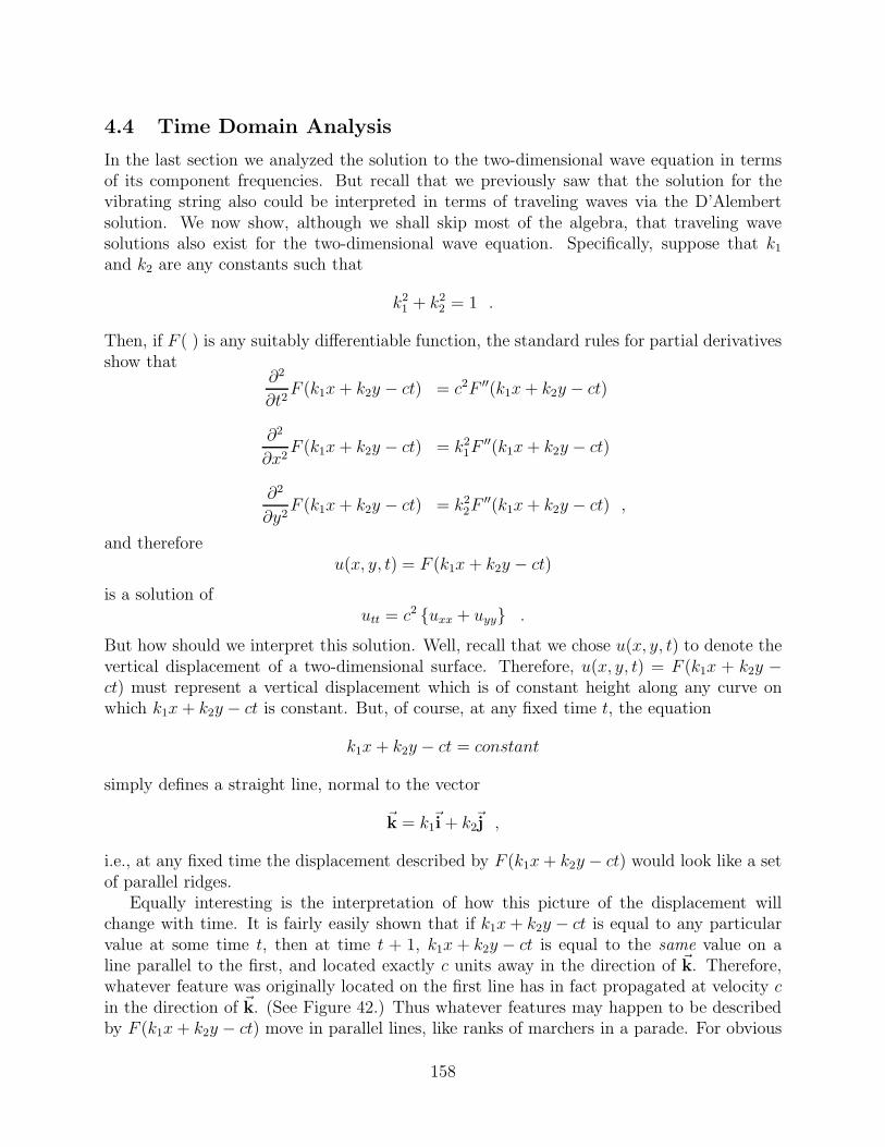
4.4 Time Domain Analysis

In the last section we analyzed the solution to the two-dimensional wave equation in termsof its component frequencies. But recall that we previously saw that the solution for thevibrating string also could be interpreted in terms of traveling waves via the D’Alembertsolution. We now show, although we shall skip most of the algebra, that traveling wavesolutions also exist for the two-dimensional wave equation. Specifically, suppose that k1

and k2 are any constants such that

k21 + k2

2 = 1 .

Then, if F ( ) is any suitably differentiable function, the standard rules for partial derivativesshow that

∂2

∂t2F (k1x+ k2y − ct) = c2F ′′(k1x+ k2y − ct)

∂2

∂x2F (k1x+ k2y − ct) = k2

1F′′(k1x+ k2y − ct)

∂2

∂y2F (k1x+ k2y − ct) = k2

2F′′(k1x+ k2y − ct) ,

and thereforeu(x, y, t) = F (k1x+ k2y − ct)

is a solution ofutt = c2 {uxx + uyy} .

But how should we interpret this solution. Well, recall that we chose u(x, y, t) to denote thevertical displacement of a two-dimensional surface. Therefore, u(x, y, t) = F (k1x + k2y −ct) must represent a vertical displacement which is of constant height along any curve onwhich k1x+ k2y − ct is constant. But, of course, at any fixed time t, the equation

k1x+ k2y − ct = constant

simply defines a straight line, normal to the vector

�k = k1�i + k2

�j ,

i.e., at any fixed time the displacement described by F (k1x+ k2y − ct) would look like a setof parallel ridges.

Equally interesting is the interpretation of how this picture of the displacement willchange with time. It is fairly easily shown that if k1x+ k2y − ct is equal to any particularvalue at some time t, then at time t + 1, k1x+ k2y − ct is equal to the same value on aline parallel to the first, and located exactly c units away in the direction of �k. Therefore,whatever feature was originally located on the first line has in fact propagated at velocity cin the direction of �k. (See Figure 42.) Thus whatever features may happen to be describedby F (k1x+ k2y − ct) move in parallel lines, like ranks of marchers in a parade. For obvious

158

0 0.5 1 1.5 20 0.5 1 1.5 20

1

2

3

4

0 0.5 1 1.5 20 0.5 1 1.5 20

1

2

3

4

0 0.5 1 1.5 20 0.5 1 1.5 20

1

2

3

4

Figure 42: A Traveling Plane Wave

reasons, such motion is commonly called a plane wave. That such solutions should exist forthe two-dimensional wave equation should not actually be that surprising. It’s really justthe analog of the D’Alembert solution for the one-dimensional string - with one fundamentaldifference. On the one-dimensional string there are exactly two traveling waves - one movingto the left, and the other to the right. By contrast, the two-dimensional wave equation canhave an infinite number of simultaneous independent plane wave solutions, since there are aninfinite number of different possible choices for �k. Figure 43 displays a solution consisting ofthe superposition of two wave traveling in different, but not opposite directions. One of thewaves consists of two crests, and is moving generally from left to right. The second consistsof a single crest, and is moving more or less toward the reader.

We shall not pursue this line of investigation any further. The actual mechanics ofdecomposing an arbitrary two-dimensional initial displacement into a sum of plane waves isfar more involved than the one-dimensional D’Alembert decomposition into two half-heightcopies of the initial displacement, and beyond the scope of these notes. We are simply contentto have observed that the rectangular membrane enjoys the same dual frequency domain,time-domain nature that we discovered for the vibrating string. Furthermore, as with thestring, which nature dominates in a particular problem depends on both the problem and thephenomenon being considered. The frequency domain view answers why drums and violinsdo not sound alike. The time domain view explains how the sound from either instrumentpropagates across a room to a listener’s ear.

4.5 The Wave Equation in Circular Regions

We turn now to the physically more realistic, and mathematically more challenging problemof describing the vibrations of a circular membrane (i.e. a standard drum). The natural

159

0 0.5 1 1.5 20 0.5 1 1.5 2

0

2

4

6

0 0.5 1 1.5 20 0.5 1 1.5 2

0

2

4

0 0.5 1 1.5 20 0.5 1 1.5 2

0

2

4

Figure 43: Two Plane Waves Traveling in the Directions k and k

coordinate system, of course, in which to formulate this problem is polar (or cylindrical)coordinates. Furthermore, as we have already noted, in this coordinate system the two-dimensional wave equation becomes

∂2u

∂t2= c2

{1

r

∂

∂r

[r∂u

∂r

]+

1

r2

∂2u

∂θ2

}. (4.5.16)

Qualitatively, this problem retains some similarities to the rectangular membrane, mostnotably in that it is still second order with respect to t, r and θ. However, it has onenew, striking dissimilarity. The original two-dimensional wave equation, written in terms ofthe Laplacian, represented a uniform membrane and had constant coefficients. In (4.5.16),however, as a direct consequence of our expressing the Laplacian in cylindrical coordinates,we have a variable coefficients partial differential equation. Although we shall not prove so,the appearance of such variable coefficients can be shown to be not an isolated occurrence,but an expected outcome of expressing the Laplacian in other than rectangular coordinates.

The appearance of these variable coefficients is not particularly auspicious! After all, ourexperience with ordinary differential equations should have shown that moving from constantcoefficient problems to variable coefficient ones caused a significant increase in computationaldifficulty, since the solutions were no longer simple exponentials, but usually some kind ofgeneral infinite series. (This difficulty, however, was still far less than that encounteredwith nonlinear differential equations.) But, first things first! Before we can even talk aboutsolving this problem, we must again address the fact that any differential equation, in andof itself, represents an incomplete problem. Moreover, based on now familiar arguments, itseems that to convert (4.5.16) into a complete problem will require defining two boundaryconditions in r, two boundary conditions in θ, and two initial conditions in t. Specifyingthe latter (i.e. appropriate initial conditions for this problem) is not a challenge. As before,

160

they will simply be the initial position and velocity, i.e.

u(r, θ, 0) = f(r, θ)ut(r, θ, 0) = g(r, θ)

However, deducing the appropriate boundary conditions for this problem is not quiteso straightforward. After all, the circular drum has only one physical boundary, the outeredge (r = L)! For any normal drum, of course, this outer edge is firmly clamped to theframe of the drum, which clearly implies that the boundary condition

u(L, θ, t) = 0

is appropriate. But where is the other boundary in r? And where do the two boundaryconditions in θ come from?

In order to understand how these “missing” boundary conditions are developed, we needto first appreciate one fundamental and basic fact. This fact is that while this problem hasonly one physical boundary, there are really three other mathematical boundaries - placeswhich, while they do not coincide with a physical ending of the medium, nevertheless cannotbe crossed, any more than we can cross the boundary at r = L without leaving the drum.(We shall see precisely where these boundaries are shortly.) Physically, these other bound-aries are artifices of the particular coordinate system involved. Nevertheless, the differentialequation sees them as completely real. Furthermore, as we shall now see, these mathematicalboundaries in fact introduce precisely the conditions necessary to ensure that (4.5.16) havea unique solution.

The first such mathematical boundary occurs at r = 0, for, by convention the radiuscannot take on negative values in cylindrical coordinates. Any situation that might math-ematically, lead to a negative radius is taken care of by keeping the radius positive andchanging the angle (θ) by 180o. (In nautical terms, for example, one would never hear ofanother ship being sighted at “bearing twenty, range minus ten miles.”) But since r = 0is a boundary, what conditions are appropriate there? The answer to this question is fairlyeasy to deduce, at least for the circular drum. The fundamental requirement, here and in allsimilar situations, is that mathematical boundaries may not introduce physically unrealisticsolutions into the problem. But how does this produce a boundary condition at r = 0?

Well, as we noted earlier, the partial differential equation (4.5.16) becomes singular at theorigin. Moreover, as is well-known, at least in the study of ordinary differential equations,singular points in the differential equation may cause corresponding singularities in thesolutions themselves. However a singular solution would imply an infinitely large verticaldisplacement at the center of the drum, which would clearly be physically unrealistic. Equallyunacceptable would be a solution whose gradient became singular at the center. Therefore,we must now pose a boundary condition which ensures that such solutions will not occurmathematically in the solution to (4.5.16). One such condition is

u(0, θ, t),∂u

∂r(0, θ, t) are finite .

(This condition actually involves a bit of “overkill.” Simply requiring that u(0, θ, t) be finitewill turn out to have been sufficient to produce the correct solutions in all cases we shall

161

consider.) Thus we now have our second boundary condition in r, and so may turn todeveloping the appropriate boundary conditions in angle.

The mathematical boundaries in θ also arise because of convention related to the coordi-nate system. Specifically, in polar coordinates, the values of θ are restricted to lie in a 360o

range, e.g. from −π to π. Any mathematical calculation which would produce an angleoutside of this range is taken care of by increasing or decreasing the argument by a sufficientmultiple of 2π to bring it back into the acceptable range. (For example, θ = 760o is resetto 40o.) This restriction in effect introduces boundaries at θ = −π and θ = π. (Actually, wecould equally well place these boundaries at 0 and 2π. This would make no difference in thecondition we shall develop.) But, mathematically, how do we ensure the solutions to (4.5.16)recognize this? One way is to impose a periodicity restriction

u(r, θ, t) = u(r, θ + 2π, t) . (4.5.17)

(This condition simply says that because the points (r, θ) and (r, θ + 2π) are physicallyidentical, then the solutions there must also be identical.) But wait! Didn’t we say weneeded two boundary conditions in θ ?

Well, we did. And this periodicity condition actually does lead to two conditions in θ,although this last fact is probably not obvious! The reason is that we can evaluate (4.5.17)at θ = −π, yielding

u(r, π, t) = u(r,−π, t) ,

and then take a partial derivative of the same condition with respect to θ, and evaluate thatderivative also at θ = −π to yield the second condition:

uθ(r, π, t) = uθ(r,−π, t) .

Thus we in fact have two boundary conditions in θ, although we shall choose to still use theperiodicity condition since it is slightly simpler to write and to understand.

Since we now appear to have developed the requisite number of boundary conditions,we should therefore have enough information to ensure the existence of a unique solutionto (4.5.16). So we simply combine all of these various pieces into the following completeproblem for the circular drum

∂2u

∂t2= c2

{1

r

∂

∂r

[r∂u

∂r

]+

1

r2

∂2u

∂θ2

}

u(0, θ, t),∂u

∂r(0, θ, t) are finite

u(L, θ, t) = 0u(r, θ, t) = u(r, θ + 2π, t)u(r, θ, 0) = f(r, θ)ut(r, θ, 0) = g(r, θ)

(4.5.18)

As it turns out, this is still a fairly difficult conceptual and computational problem. There-fore, in the next section, we shall restrict ourselves to investigating the solution of a slightlysimpler special case of it.

162

4.6 Symmetric Vibrations of the Circular Drum

In these notes, we shall solve in detail only one special case of the wave equation for cir-cular regions. This case nevertheless exhibits the most important aspects of this problem -especially those aspects which are new and different compared to properties of solutions inrectangular regions. The special case we shall study is that of symmetric vibrations, i.e.those which are independent of angle. (Such vibrations should arise, due to symmetry, if, forexample, a drum were struck precisely in its center.) The boundary value problem which de-scribes such vibrations may be found simply by dropping all of the angle-related dependencein (4.5.18) and setting all derivatives with respect to angle equal to zero. This yields

∂2u

∂t2= c2

1

r

∂

∂r

[r∂u

∂r

]

u(0, t),∂u

∂r(0, t) are finite

u(L, t) = 0u(r, 0) = f(r)ut(r, 0) = g(r)

(4.6.19)

Like the simple vibrating string, this problem involves precisely two independent vari-ables, r and t. Furthermore, like the string, the partial differential equation here possess anatural splitting - only time operations on the left, and only spatial operations on the right.Therefore, using the by-now familiar logic of separation of variables, we shall assume thatthe homogenous solutions, i.e. the solutions to

∂2u

∂t2= c2

1

r

∂

∂r

[r∂u

∂r

]

u(0, t),∂u

∂r(0, t) are finite

u(L, t) = 0

(4.6.20)

have the formu(r, t) = R(r)T (t) .

Substituting this product into the partial differential equation and then dividing by theproduct c2R(r)T (t) yields

T ′′(t)c2T (t)

=(rR′(r))′

rR(r)= −λ .

Here, as before, we introduce the separation constant (λ) because of the standard argument -the left hand side is independent of r and the right hand side is independent of t. (The minussign is included to conform to our earlier experience.) This last equation can then be writtenas the two equivalent equations

T ′′ + λc2T = 0 and (rR′)′ + λrR = 0 ,

163

where we have again chosen to suppress the explicit dependence on the variables.At this point, both of these differential equations are, in theory, solvable for any value

of λ. But, of course, as we have also seen before, that is because we have not yet appliedour separation assumption to the full homogeneous problem, i.e. we must still separate theboundary conditions. In terms of the separated form, the condition at the origin becomes

u(0, t) = R(0)T (t) is finite, and∂u

∂r(0, t) = R′(0)T (t) is also finite,

which clearly impliesR(0), R′(0) are finite,

or stated more compactlyR(0), R′(0) finite.

The boundary condition at the outer rim of the drum is identical to that in Dirichlet condi-tions on the string, and separates similarly

u(L, t) = R(L)T (t) = 0⇒ R(L) = 0 .

Thus, the complete homogenous problem for the separation form solutions becomes

T ′′ + λc2T = 0 (rR′)′ + λrR = 0R(0), R′(0) finite

R(L) = 0(4.6.21)

By now, the next step should be fairly obvious. We must determine the eigenvalues andeigenfunctions of

(rR′)′ + λrR = 0R(0), R′(0) finite

R(L) = 0(4.6.22)

Before we look at the details of solving this problem, there are a few general observationswe should make. First of all, in one important aspect this problem is radically differentfrom all of our earlier cases - the ordinary differential equation is not constant coefficient.(As we noted earlier, this is a direct consequence of the representation of the Laplacian innonrectangular coordinates.) Equally important, however is the fact that, even with thisadded twist, the problem is still Sturm-Liouville, although of a slightly different type thanwe have encountered before. (The correspondence to the standard Sturm-Liouville form

[p(x)y′(x)]′ + [λw(x)− q(x)]y(x) = 0 , 0 < x < L

is x = r, y(r) = R(r), p(r) = r, w(r) = r,and q(r) ≡ 0.) It is, however, not a regularproblem, in the sense we defined in the previous chapter, because it violates the conditionthat p(x) should be positive on the entire interval, including the end points, but is anexample of what is called a singular Sturm-Liouville problem. Nevertheless, its solutions canbe shown to possess essentially all of the same properties as we found for solutions of the

164

regular problem. Thus, for example, there will be no negative eigenvalues. Furthermore, zerowill not be an eigenvalue, because a nonzero constant cannot satisfy the boundary conditionat r = L. Moreover, there will be an infinite number of positive eigenvalues, λn = ξ2

n →∞as n→∞. Lastly, each eigenfunction will have one more zero in the interval 0 < r < L thandid its predecessor. And all of these conclusions can be made even before we know the formof the general solution to the variable coefficient ordinary differential equation involved!

We are however, still left with the problem of calculating the specific eigenvalues andeigenfunctions of (4.6.22) when λ > 0. Conceptually, this could be reasonably difficultgiven the variable coefficient nature of the differential equation. According to the theory ofordinary differential equations, we would have to assume a general power series solution, i.e.

R(r) =∞∑

n=0

anrn+p ,

and then substitute this form into the differential equation to determine the value(s) of pand the recurrence relation for the coefficients. Fortunately, we will not have to carry out allof these steps here, because the ordinary differential equation which appears in this problemhas already been extensively studied. This equation, which we shall rewrite in the equivalentform

r2R′′ + rR′ + λr2R = 0 (4.6.23)

is called Bessel’s12 equation of order zero. (Appendix A.) The general solution to this probleminvolves two linearly independent functions (as does the general solution to any secondorder linear ordinary differential equation). These solutions are normally represented by thesymbols J0(ξr) and Y0(ξr), and called the ordinary Bessel functions of the first and secondkinds, of order zero, respectively. Both of them can be calculated using infinite series whichconverge for all values of r, and most standard computer systems include programs which willcompute their values. Their graphs are shown at Figure 44. For our purposes, we shall treatthese functions as somewhat like “black boxes,” in that every time we encounter (4.6.23), weshall simply proceed to write its general solution as a linear combination of J0(ξr) and Y0(ξr)with the full assurance that these functions could be calculated whenever required, eventhough we may not at this point fully appreciate the exact mechanisms by which thosecalculations would be made. (This approach may seem a bit troubling, and perhaps shouldbe, at least initially. However, you might reflect that, to a fair degree, we really do littlemore than this when we write the solution to

y′′ + ξ2y = 0 as y(x) = a1 cos(ξx) + a2 sin(ξx) ,

for, after all, what do we really immediately know about the sine and cosine except

• What their graphs look like,

• That their values can be obtained either by using a calculator (or computer), or fromtables, and

12Friedrich Wilhelm Bessel,see http://www-gap.dcs.st-and.ac.uk/∼history/Mathematicians/Bessel.html

165

• That they satisfy certain identities?

For example, do you really know how that chip inside your pocket calculator arrives at avalue when you hit the SIN key? You probably don’t, and it’s really not all that important.What is crucial is that those values are accurate and you can use them in calculations! Weshall adopt a similar view toward Bessel functions.)

0.80.6

0.4

0-0.2

x

20151050

1

0.2

-0.4

Y_0

J_0

Figure 44: The Ordinary Bessel Functions J0(r) and Y0(r)

Since, as noted above, we can now represent the general solution to the differentialequation in (4.6.22) (with λ = ξ2) as

R(r) = a1J0(ξr) + a2Y0(ξr) . (4.6.24)

We must now determine the exact eigenvalues by applying the boundary conditions to thissolution. Referring to Figure 44, we see that Y0(ξr) is singular at the origin, therefore itcannot satisfy the boundary condition at r = 0, and thus it cannot appear in the solutioni.e.

R(0), R′(0) finite⇒ a2 = 0 .

(Note we could not make a similar conclusion in any case which did not include the originas part of the physical region, e.g. if we were to build a “donut-shaped” drum. But in sucha region, there would be a second real physical boundary (at the inner radius), and hencewe would not have needed the finiteness condition anyway.)

Finally, the remaining boundary condition in (4.6.22) yields

R(L) = 0⇒ a1J0(ξL) = 0⇒ J0(ξL) = 0 . (4.6.25)

Sturm-Liouville theory and the general shape of the graph of J0(r) in Figure 44 assure us thatthere will be an infinite number of different values of ξ which satisfy this condition. In fact,every axis crossing of J0(r) in that figure will generate another solution of (4.6.25), in thesame way that every axis crossing of the curve of sin(x) generated another integer multiple

166

of π, and another solution of sin(ξL) = 0 in the vibrating string problem. Really the onlydifference between solving (4.6.25) and determining the eigenvalues of the one dimensionalstring problem is that, unfortunately, there is no convenient general formula (such as nπ)that describes the roots of J0(r) = 0, and therefore no convenient formula for representingthe solutions of J0(ξL) = 0. They can only be listed, e.g.

ξ1L = 2.4048 , ξ2L = 5.5201 , ξ3L = 8.6537 , · · ·

or

ξ1 =2.4048

L, ξ2 =

5.5201

L, ξ3 =

8.6537

L, · · · (4.6.26)

Again, we choose to view this as more of a notational inconvenience than a computationaldrawback, and therefore conclude that we have found the eigenfunctions for the problem

Rn(r) = J0(ξnr) , n = 1, 2, . . . (4.6.27)

with the ξn as defined above. (Furthermore, and we shall need to use this shortly, Sturm-Liouville theory also assures that these eigenfunctions will be orthogonal with respect to theweighting function w(r) = r, i.e. that

∫ L

0rJ0(ξnr)J0(ξmr)dr = 0 , m = n . (4.6.28)

Lastly, these eigenfunctions are guaranteed to be complete in the sense that we can use themto expand any piecewise smooth function defined on 0 < r < L in a Fourier-like series.)

Of course, with the eigenfunctions in hand, we have still not completely identified thelinearly independent solutions to the homogeneous partial differential equation. We needalso to solve for the T (t). But this isn’t really very difficult, since we know, according to ourabove development and (4.6.21) that the T (t) must satisfy the equation

T ′′n + ξ2

nc2Tn = 0 . (4.6.29)

Therefore, as before, there will be two linearly independent time solutions, which we representas

Tn(t) = An cos (ξnct) +Bn sin (ξnct) . (4.6.30)

Thus, in the usual way, the general solution to (4.6.20) can be formally written

u(r, t) =∞∑

n=1

{An cos (ξnct) +Bn sin (ξnct) }J0(ξnr) . (4.6.31)

Of course, by calling this the general solution we mean it satisfies not only the homogeneouspartial differential equation and the boundary conditions, but also should, for the correctchoice of An and Bn, be able to satisfy any appropriate initial conditions.

Trying to fit the initial conditions in the original boundary value problem (4.5.18) withthis solution requires substituting t = 0 into (4.6.31) and its partial derivative with respect

167

to t, and leads to:

u(r, 0) =∞∑

n=1

AnJ0(ξnr) = f(r) ,

ut(r, 0) =∞∑

n=1

ξncBnJ0(ξnr) = g(r) .

(4.6.32)

These two equations really represent the same general problem. The only difference is thatthe effective coefficient in the second initial condition is not An, but ξncBn. Thus we shallfocus on determining the coefficients in the first initial condition, with the assurance thatwhatever approach will find the coefficients in that problem could be immediately appliedto find the coefficients in the initial velocity condition.

Of course, were it not for Sturm-Liouville theory, finding a formula for the coefficientsin (4.6.32) could be a formidable task. But because this theory assures us that sincethe J0(ξnr) are orthogonal, we can apply the general Sturm-Liouville coefficient formula(given by (3.10.57) in Chapter 3) directly. Equivalently, we could in the usual way multiplyboth sides of (4.6.32) by rJ0(ξmr), where m denotes some fixed integer, and then integrateyielding ∫ L

0rf(r)J0(ξmr)dr =

∞∑n=1

An

∫ L

0rJ0(ξnr)J0(ξmr)dr︸ ︷︷ ︸

= 0 , m�=n

,

and then apply the orthogonality property. Both approaches will lead to the same formula

An =

∫ L

0rf(r)J0(ξnr)dr∫ L

0r [J0(ξnr)]

2 dr. (4.6.33)

So we can formally compute the An! (A similar set of steps can be shown to produce thefollowing formula for the Bn

Bn =

∫ L

0rg(r)J0(ξnr)dr

ξnc∫ L

0r [J0(ξnr)]

2 dr.) (4.6.34)

You should appreciate (and almost certainly do) that these integrals will generally not beelementary, i.e. the antiderivatives will not be found in most standard calculus texts. Inmost cases, the antiderivatives may not even be known, and therefore the values of thevarious coefficients would have to be done numerically, e.g. by Simpson’s rule. Nevertheless,mathematically, the results of Sturm-Liouville theory ensure us that (4.6.32) is really a validset of equalities, and that, using the coefficients computed by (4.6.33)-(4.6.34) will satisfy theinitial condition, provided the J0(ξnr) include all of the linearly independent eigenfunctionsof the associated Sturm-Liouville problem which comes from separation of variables. Thiseffectively completes the solution of (4.5.18).

168

We close this section with a brief example illustrating the above method

∂2u

∂t2=

1

r

∂

∂r

[r∂u

∂r

], 0 < r < 4 , 0 < t

u(0, t),∂u

∂r(0, t) finite

u(4, t) = 0

u(r, 0) =

(1− r2

16

)ut(r, 0) = 0

This represents a circular drum, of radius four, with a tension and density such that c2 = 1.There is an initial displacement, but no initial velocity. According to the above development,the eigenfunctions are

Rn(r) = J0(ξnr) , n = 1, 2, . . . ,

where the eigenvalues are determined by

J0(4ξn) = 0 , n = 1, 2, . . . ,

and thus have the values

ξ1 = 0.6012 , ξ2 = 1.3800 , ξ3 = 2.1634 ,

ξ4 = 2.9479 , ξ5 = 3.7327 , ξ6 = 4.5178 , · · · .

The general solution is then (since c2 = 1)

u(r, t) =∞∑

n=1

{An cos (ξnt) +Bn sin (ξnt) }J0(ξnr) ,

with the ξn as given. The initial conditions reduce to

u(r, 0) =∞∑

n=1

AnJ0(ξnr) = 1− r2

16,

ut(r, 0) =∞∑

n=1

ξnBnJ0(ξnr) = 0⇒ Bn = 0 ,

or,

u(r, t) =∞∑

n=1

An cos (ξnt) J0(ξnr) ,

where, according to (4.6.33)

An =

∫ 4

0r(1− r2/16)J0(ξnr)dr∫ 4

0r [J0(ξnr)]

2 dr.

169

Numerical integration could show

A1 =

∫ 4

0r(1− r2/16)J0(.6012r)dr∫ 4

0r [J0(.6012r)]2 dr

= 1.1080

A2 =

∫ 4

0r(1− r2/16)J0(1.3800r)dr∫ 4

0r [J0(1.3800r)]2 dr

= −0.1398

A3 =

∫ 4

0r(1− r2/16)J0(2.1634r)dr∫ 4

0r [J0(2.1634r)]2 dr

= 0.0455

A4 =

∫ 4

0r(1− r2/16)J0(2.9479r)dr∫ 4

0r [J0(2.9479r)]2 dr

= −0.0210

A5 =

∫ 4

0r(1− r2/16)J0(3.7327r)dr∫ 4

0r [J0(3.7327r)]2 dr

= 0.0116

A6 =

∫ 4

0r(1− r2/16)J0(4.5178r)dr∫ 4

0r [J0(4.5178r)]2 dr

= −0.0072 , . . . .

4.7 Frequncy Domain Analysis of the Circular Drum

In the previous section, we showed that the vibrations of a circular membrane, fixed at theouter edge and with a non-zero initial displacement but no initial velocity, are given by

u(r, t) =∞∑

n=1

An cos (ξnct) J0(ξnr) ,

where the ξn are defined by

J0(ξnL) = 0 , n = 1, 2, . . . .

As was the case with both the vibrating string and the rectangular membrane, we mayrewrite this solution as

u(r, t) =

[A1J0(ξ1r)

]cos (ξ1ct) +

[A2J0(ξ2r)

]cos (ξ2ct) +

[A3J0(ξ3r)

]cos (ξ3ct) + · · · ,

170

i.e. as a sum of standing vibrations, each vibrating with a different frequency

fn =ξnc

2π, n = 1, 2, . . . .

The various modes of this vibration are, as before, simply the eigenfunctions of the problem

J0(ξnr) , n = 1, 2, . . . .

The first four of these are plotted in Figure 45. (This figure actually plots a full cross sectionof the membrane, where the negative points, in polar coordinates, really mean a change inangle of 180o.) Their shape is similar to that of the modes in the fixed end vibrating string,although not all of the “peaks” in any one mode have the same height.

−1.2

1

1.2

n=1

−1.2

1

1.2

n=2

−1.2

1

1.2

n=3

−1.2

1

1.2

n=4

Figure 45: Modes of the Circular Membrane

The natural frequencies of the circular membrane are determined, except for a scalefactor of c/2π, by the zeros of the Bessel function. But as we have already discussed atsome length, these zeros are not uniformly spaced along the horizontal axis. Therefore, thespectrum of the circular membrane, like that of the rectangular membrane, will lack theregular picket fence structure of the spectrum of the vibrating string. However, the degreeto which the circular membrane’s frequencies are not evenly spaced is not as pronounced asis the case with the rectangular membrane. This is illustrated by Figure 46, which plots thefrequencies of the circular membrane. One must look fairly closely at this figure to see theuneven spacing. Nevertheless, they are not evenly spaced and therefore, while which wouldsound “better” is clearly a matter of personal taste, the unmistakable conclusion is that acircular drum will not sound like a violin!

4.8 Time Domain Analysis of the Circular Membrane

A complete analysis of the structure of traveling waves in cylindrical coordinates is beyondthe scope of our discussion here. Nevertheless, we claim that such an interpretation ispossible, and that circular traveling waves in fact exist. For the proof of this, one need onlydrop a small stone into a small, flat pond of water and observe the resulting motion.

171

0 2 4 6 8 10 12 14 160

0.2

0.4

0.6

0.8

1

3.1153 3.1336 3.1378 3.1394

Figure 46: Spectrum of the Circular Membrane

172

PROBLEMS

1. It can be shown that the small free vertical vibrations of a uniform beam (e.g. a bridgegirder) are governed by the fourth order partial differential equation:

∂2u

∂t2+ c2

∂4u

∂x4= 0

where c2 is a constant involving the elasticity, moment of inertia, density and cross sectionalarea of the beam. If the beam if freely supported at both ends, e.g. sitting on a piling, theboundary conditions for this problem become:

u(0, t) = u(L, t) = 0uxx(0, t) = uxx(L, t) = 0

Show that separation of variables “works” in this problem, and, in case the beam is initiallyat rest, i.e.

ut(x, 0) = 0

produces a general solution of the form:

∞∑n=1

An cos

(n2π2ct

L2

)sin

(nπx

L

)

2. Solve the two-dimensional rectangular wave equation:

utt = uxx + uyy

u(0, y, t) = u(1, y, t) = 0u(x, 0, t) = u(x, 1, t) = 0u(x, y, 0) = .01xy(1− x)(1− y)ut(x, y, 0) = 0

3. Solve the two-dimensional rectangular wave equation:

utt = 16 (uxx + uyy)u(0, y, t) = u(3, y, t) = 0u(x, 0, t) = u(x, 2, t) = 0

u(x, y, 0) = y(2− y) sin(

2πx3

)ut(x, y, 0) = 0

173

4. Find the eigenvalues and the form of the eigenfunctions for:

utt = 9 (uxx + uyy)u(0, y, t) = u(4, y, t) = 0uy(x, 0, t) = u(x, 1, t) = 0

Calculate the actual values of the four lowest natural frequencies.

5. One of the “quirks” of the two-dimensional wave equation in rectangular coordinates isthat, unlike the one-dimensional problem, two different values of n and m may yield thesame natural frequency, and therefore this single natural frequency may have two (or more)independent modes (“shapes”) associated with it. For example, if L = 2 and W = 1, theeigenvalues and eigenfunctions are,

λnm =[(

n2

)2+m2

]π2

and

unm = sin(mπy) sin(

nπx2

).

Show that the following eigenvalues are in fact equal:

λ41 = λ22 ; λ61 = λ23 ; λ62 = λ43 ; λ72 = λ14

6. Show that in the square membrane, certain natural frequencies may have four independentmodes (“shapes”) associated with them.

174

PROBLEMS

1. Show that separation of variables (u(r, θ, t) = R(r)Θ(θ)T (t)), applied to the wave equationin a circular region of radius A,

∂2u

∂t2= c2

{1

r

∂

∂r

[r∂u

∂r

]+

1

r2

∂2u

∂θ2

}

u(A, θ, t) = 0

u(0, θ, t) ,∂u

∂r(0, θ, t) finite

u(r, θ, t) = u(r, θ + 2π, t)

leads to

T ′′ + λc2T = 0 r [rR′]′ + (λr2 − µ)R = 0 Θ′′ + µΘ = 0R(0) , R′(0) finite Θ(θ) = Θ(θ + 2π)R(A) = 0

2. Explain the mathematical and physical significance of the condition

u(r, θ, t) = u(r, θ + 2π, t).

3. Find the three lowest natural frequencies of

utt =6

r

∂

∂r

[r∂u

∂r

]

u(4, t) = 0

u(0, t) ,∂u

∂r(0, t) finite

u(r, 0) = f(r)ut(r, 0) = 0

You need the Appendix to solve the following two problems.

4. Using the recurrence formulas, and a table of values for J0(x) and J1(x), find

a. J ′1(x) in terms of J0(x) and J1(x)

b. J2(2.0)

c. J ′3(1.0)

175

5. Write, in terms of Jn(x) and Yn(x), the general solution to

a. x2y′′ + xy′ + 4x2y = 0

b. x2y′′ + xy′ + (9x2 − 4)y = 0

c. 4x2y′′ + 4xy′ + (x2 − 1)y = 0

6. Solve the following problems. (Non-zero coefficients may be left in terms of definiteintegrals of known functions.)

a.

utt =1

r

∂

∂r

[r∂u

∂r

]

u(2, t) = 0

u(0, t) ,∂u

∂r(0, t) finite

u(r, 0) = sin(πr)ut(r, 0) = 0

b.

utt =4

r

∂

∂r

[r∂u

∂r

]

u(1, t) = 0

u(0, t) ,∂u

∂r(0, t) finite

u(r, 0) = 1− r2

ut(r, 0) = 0

c.

utt = c21

r

∂

∂r

[r∂u

∂r

]

u(2, t) = 0

u(0, t) ,∂u

∂r(0, t) finite

u(r, 0) = 0ut(r, 0) = 1

7. Solve the following problem. (Non-zero coefficients may be left in terms of definiteintegrals of known functions.) Physically interpret the boundary conditions, and relate this

176

to the properties of the solution:

utt = c21

r

∂

∂r

[r∂u

∂r

]

ur(L, t) = 0

u(0, t) ,∂u

∂r(0, t) finite

u(r, 0) = f(r)ut(r, 0) = 0

177

5 Introduction to the Fourier Transform

5.1 Periodic and Aperiodic Functions

Thus far in our study we have focused on developing an understanding of the propertiesand uses of the Fourier series (and its immediate relatives). Almost from the beginningwe have seen the power of Fourier series as a tool for both decomposing and constructinggeneral (usually complicated) periodic functions in terms of “pure” sines and cosines, andwe have seen how these series provide significant insights into the physical world. Thephysical world, however, is full of interesting aperiodic functions as well as periodic ones.In fact, a cynic might well argue “Only the aperiodic functions are real. A truly periodicfunction must continue, unabated, for all time, which clearly requires infinite energy, andtherefore the existence of such functions is impossible.” (For example, as any astronomerwill attest, even the Sun itself is actually “running down” - losing energy every day!) Thepragmatist, of course, would likely counter “So what! Mathematical physics is based onmodeling approximations, neglecting small terms, etc. As long as we can model an aperiodicfunction sufficiently closely with a periodic one (or vice versa), what’s the harm? Moreover,if it takes a million years to tell the difference, who’s going to notice!”

The degree to which the Fourier series results we’ve studied so far do agree with observedphysical behavior argues strongly that we have not in fact made any unwarranted approx-imations. Therefore, since aperiodic functions are a very real fact of life, in the comingsections we shall study how they and their properties relate, in the Fourier sense, to thoseof the periodic functions.

We start by considering how we might represent an arbitrary, aperiodic function. Weshall denote this function as h(t). (We choose not to call it f(t) for two reasons. First, wewish to reinforce the notion that not all functions use the letter f . Secondly, we are later ongoing to want to use the letter f to stand for a different physical quantity.) But since h(t) isnot periodic, we cannot represent it in terms of a Fourier series - at least not immediately.So how do we start?

We shall take an approach which generally produces valid results in applied mathematics -combine a bit of common sense with an appeal to physical “reasonableness.” Specifically,we introduce a “new” function, denoted h(t), with the properties that

(1) h(t) is periodic, of period 2L,

(2) L is “large,” and

(3) h(t) and h(t) are identical for −L < t < L.

Our idea, of course, is that if L is sufficiently large, say a million years, then for all practicalpurposes h(t) and h(t) will be indistinguishable. Moreover, reason says that the larger Lbecomes, the closer their mathematical representations should become. This suggests that,mathematically, we consider the limit of h(t) as L→∞. (After all, this is a mathematicstext!) In this limit, h(t) and h(t) should become physically identical, and therefore, by all

178

reason, the limit of any mathematical representation we’ve developed for h(t) should alsorepresent h(t). But, of course, if we are to do all of this, we must first have a representationfor h(t)! (You should appreciate that, in practical problems, we would also first need to havea strong understanding of the time scales of the dominant physical processes, since termssuch as “large” or “small” really have meaning only in a relative sense. For example, a hourwould clearly be a very large time for the analysis of a single radar pulse, while a millionyears might actually be too short to examine an astronomical phenomenon!)

5.2 Representation of Aperiodic Functions

Deriving a representation for h(t) is not difficult. After all, we’ve assumed that it is periodic!We can therefore simply express it as Fourier series, and this is exactly what we shall do,albeit with one slight “twist” - we’ll use the complex form of the series. (The reason for thisis primarily convention. Almost all other texts develop a complex-valued representation foraperiodic functions. You should rest assured that a completely identical, if somewhat morecumbersome representation could be derived from the real form of the Fourier series.) Thecomplex form of the Fourier series, as we have already shown, is:

h(t) =∞∑

n=−∞cne

jnπt/L (5.2.1)

where (in deference to the convention of most signal processing texts) we now use j to standfor√−1 , and the coefficients,

cn =1

2L

∫ L

−Lh(t)e−jnπt/Ldt =

1

2L

∫ L

−Lh(t)e−jnπt/Ldt (5.2.2)

represent the (complex) amplitudes of the various component frequencies which make up h(t).(Note the use of our assumption that h(t) and h(t) are identical for −L < x < L.) If we nowuse (5.2.2) to substitute for cn in (5.2.1) (naturally changing to some dummy variable ofintegration other than t), we have:

h(t) =∞∑

n=−∞

1

2L

{∫ L

−Lh(u)e−jnπu/Ldu

}ejnπt/L (5.2.3)

We now modify this representation slightly by introducing the change of variables

∆ω =π

Land ωn =

nπ

L. (5.2.4)

(This change really involves nothing particularly new - ωn is simply the nth radian frequencyand ∆ω the difference between two such adjacent frequencies in the representation for h(t).)With these new variables, the series representation now becomes

h(t) =1

2π

∞∑n=−∞

{∫ L

−Lh(u)e−jωnudu

}ejωnt∆ω (5.2.5)

179

But wait! This series is now of the form,

1

2π

∞∑n=−∞

F (ωn)∆ω (5.2.6)

where

F (ωn) =

{∫ L

−Lh(u)e−jωnudu

}ejωnt

xn

y(xn)

a b

y(x)

∆ x

Figure 47: Approximation of the Definite Integral

and the form of (5.2.6) should look at least a bit familiar. For it’s very close (although as weshall see not quite identical) to the Riemann13 sum used in virtually every calculus text aspart of the introduction of the definite integral. In the Riemann sum, an interval of interest(say a ≤ x ≤ b) is first divided up into N equal segments of length ∆x (= (b− a)/N). Thenthe area under some arbitrary continuous function y(x) is approximated by the area under aset of rectangles, each of which has a base length of ∆x, and a height equal to the height ofthe curve at some value of x (denoted xn) inside the nth rectangle (Figure 47). The Riemannsum, which is just the total area under all of these rectangles, then clearly approximatesthe area under the curve. Moreover, as ∆x becomes progressively smaller, this sum shouldbecome closer and closer to the actual area. Thus, since by definition the area under thecurve is the definite integral, we then have that in Figure 47

lim∆x→0

N∑n=1

y(xn)∆x =∫ b

ay(x)dx (5.2.7)

13Georg Friedrich Bernhard Riemann,see: http://turnbull.mcs.st-and.ac.uk/history/Mathematicians/Riemann.html

180

We now choose to view this last formula as simply a formal operational procedure - i.e. toarrive at the definite integral, start with the appropriate Riemann sum, then, in the limit,replace the summation by an integral sign with the proper limits, drop the subscript on (xn),and finally replace ∆x with dx. (Of course, significant and nontrivial mathematical resultsprecede this formal procedure. One of the hardest of these is proving the limit even exists!And while we shall not concern ourselves with repeating the proofs of these results here, wemust still recognize their crucial importance to the formal procedure we deduce from (5.2.7).)

Returning now to our attempt to derive a representation for h(t), recall that we expectthe representations for h(t) and h(t) to become identical in the limit as L→∞. However,according to (5.2.4), we see that

L→∞ is equivalent to ∆ω → 0 ,

and so it seems perfectly reasonable to write

h(t) = limL→∞

h(t) = limL→∞

1

2π

∞∑n=−∞

{∫ L

−Lh(u)e−jωnudu

}ejωnt∆ω

=1

2πlim

∆ω→0

∞∑n=−∞

F (ωn)∆ω

(5.2.8)

But, since the last term in (5.2.8) now looks like the left-hand side of (5.2.7), we should beable to apply the formal procedure we’ve just described to compute these limits! (Actually,this argument glosses over a great deal of “thin” theory. The interval of integration associ-ated with (5.2.8) is −∞ < ω <∞, whereas (5.2.7) involves an interval of only finite length.Thus our integral will be improper, and so (5.2.8) represents a very non-trivial extension ofthe Riemann sum in somewhat the same way that the infinite series itself is a non-trivialextension of the usual sum. As with other similar concerns in this text, we shall not dwellon this one. We prefer, for the moment, to assume this extension will work, and see whetherthe results seem either useful or interesting, or both. If no useful results emerge from thisapproach, then whether they are valid or not becomes in essence moot. If, however, ourformal procedure does produce apparently valuable results, we should then rigorously verifythe validity of the various steps we’re taking. Such verification, however, is far beyond thelevel of this text.)

If we do assume that (5.2.8) can be treated as the limit of a “normal” Riemann sum (5.2.7),then all that remains is the mechanics. As noted in our earlier comments, the first step ofthese mechanics is to replace the summation sign in (5.2.8) with an integral. Furthermore,since the values of ωn in our summation ranges over all values from −∞ to ∞, these valuesshould become the limits on this integral. The second formal step in (5.2.7) is to drop thesubscripts in what will become the integrand. In our present case, however, the integrand-to-be is

F (ωn) =

{∫ L

−Lh(u)e−jωnudu

}ejωnt

and therefore, since we are really taking the limit as L tends to ∞, we should not only dropthe subscript (on ωn), but also replace the upper and lower limits on this inner integral by∞

181

and −∞, respectively. (Applying this argument to the inner integral here again involves astep beyond the replacements in (5.2.7), and represents another part of our derivation thatproperly requires later theoretical analysis.) The final step of our formal procedure, whichwe must apply to (5.2.8), is to replace ∆ω by dω. When we have completed all these stepsas described, (5.2.8) becomes

h(t) =1

2π

∫ ∞

−∞

{∫ ∞

−∞h(u)e−jωudu

}ejωtdω (5.2.9)

With (5.2.9) we have reached our goal of finding a representation for a general aperiodicfunction. But we’re not quite done! The reason we say this is not that (5.2.9) is not acompletely valid expression. It is! There are, however, other equivalent forms that are morecommonly seen. One of these alternative forms, defined by the change of variables

ω = 2πf , (5.2.10)

is

h(t) =∫ ∞

−∞

{∫ ∞

−∞h(u)e−2πjfudu

}e2πjftdf (5.2.11)

This is the form we shall study for the rest of this text.

5.3 The Fourier Transform and Inverse Transform

We closed the previous section when we had derived (5.2.11) as the Fourier representation fora general aperiodic function, h(t). We now consider some of the implications of this identity,and especially the similarities and differences between it and the Fourier series representationfor a periodic function. Therefore, before continuing here, you may first want to review theprevious section, concentrating especially on how each of the particular parts in (5.2.11)arose from the Fourier series for h(t) in the course of our derivation.

One immediate and striking difference between the representation of an aperiodic func-tion as given by (5.2.11) and the Fourier series representation of a periodic function, such asthe complex form given by (5.2.1) is simply that representing an aperiodic function appar-ently requires an integral instead of a series. This is consistent with our observation, madeduring the derivation in the previous section, that the difference between neighboring radianfrequencies in the series representation for h(t) was π/L. But the limiting process of letting Lgo to infinity forces this difference to approach zero, in effect squeezing the neighboring fre-quencies of h(t) closer and closer together until finally they become in essence a continuous“smear” extending across the entire frequency spectrum. Sums, of course, even infinite se-ries, are inadequate to combine values of something with respect to a continuously varyingargument - this is precisely why the definite integral appears in basic calculus courses.

In addition, we have very deliberately placed brackets inside the integral (5.2.11). Thesebrackets effectively separate that integral into two parts, and allow us, if we choose, to easilyreplace this single identity with the two separate formulae

182

H(f) =∫ ∞

−∞h(t)e−2πjft dt

and

h(t) =∫ ∞

−∞H(f)e2πjft df

(5.3.12)

(Note that this separated form also removes any need to use the dummy variable ofintegration u in the first integral. Furthermore, since t is a dummy variable in that integral,the result must be, as we have denoted, a function of only the variable f .) Choosing toexpress the identity (5.2.11) in two parts should not seem either unusual or surprising, sincethis is virtually the same thing we routinely do with Fourier series. For example, don’twe normally express the complex Fourier series with (5.2.1) and (5.2.2), rather than thecombined form (5.2.3)?

The first formula (5.3.12) in this two-part representation for aperiodic functions is com-monly called the Fourier transform (or Fourier integral transform) of h(t). Moreover, asa review of the derivation of the previous section will show, the integral in this formula isessentially the direct descendent, via the limiting process as L→∞, of the Fourier seriescoefficient (5.2.2). Therefore we shall interpret it similarly - i.e. as describing, in some sense,the amplitudes of the continuum of component frequencies that make up the aperiodic func-tion h(t), i.e. H(f) represents the (complex) amplitude of the “pure tone” of frequency ffound in h(t). Clearly then, in terms of our terminology thus far, H(f) represents thefrequency domain analysis of the time domain signal h(t).

The second formula (5.3.12) above is commonly referred to as the inverse Fouriertransform of H(f). Since we are interpreting the Fourier transform as the analog in thecase of aperiodic functions to the Fourier series coefficients for periodic functions, we thennaturally view the inverse transform as describing how to reconstruct or assemble the ape-riodic time domain signal, h(t), from the (frequency domain) knowledge of the amplitudesof its component frequencies. In other words, the second of (5.3.12) performs the identicalfunction for aperiodic functions that the Fourier series (5.2.1) itself does for periodic ones.

Calling the first of (5.3.12) the Fourier transform may bring to mind another transformyou have undoubtedly seen - the Laplace14 transform

L[h(t)] =∫ ∞

0h(t)e−stdt .

There are several similarities between the Fourier and Laplace transforms, some of whichwe shall investigate later in more detail. For the moment, we would simply note that theFourier and Laplace transforms both involve an integral depending on another variable - sfor the Laplace transform and f for the Fourier. (We must also note one significant differencebetween these two transforms - because Euler’s identity implies that the complex exponentialhas both real and imaginary parts, the Fourier transform will generally have a non-zero imaginary part even when the time-domain function (h(t)) is real, while the Laplacetransform of a real-valued function is real as long as s is.)

14Pierre-Simon Laplace,see http://www-gap.dcs.st-and.ac.uk/∼history/Mathematicians/Laplace.html

183

The Fourier and inverse Fourier transforms are sufficiently important in applications that,like the Laplace transform, they are generally given their own symbol, usually a script capitalletter. We shall follow this convention, and write

F [h(t)] = H(f) =∫ ∞

−∞h(t)e−2πjft dt (5.3.13)

andF−1[H(f)] = h(t) =

∫ ∞

−∞H(f)e2πjft df (5.3.14)

You should recognize that any specific aperiodic function h(t) is uniquely identified by itsFourier transform, just as any periodic function is uniquely identified by Fourier series coef-ficients. Therefore, for any particular function, (5.3.13) and (5.3.14) should (in fact must)be viewed as an inseparable pair, knowledge of either member of which serves to uniquelydetermine the other. (The same statement is true for Laplace transforms, and is preciselywhy tables of that transform are so useful in finding inverse transforms!) In fact, this pairingmetaphor is so central to the concept of Fourier transforms that many texts use a specialnotation, such as

h(t)↔ H(f)

to symbolize it.The Fourier transform is, however, unlike the Laplace transform in one important respect.

This difference arises because, due to their limits of integration, both the Fourier and Laplacetransforms are improper integrals. Therefore, according to the standard arguments fromthe calculus, whether the transforms of particular functions actually even exist dependson the asymptotic behavior of the integrands at these limits. However, the e−2πjft terminside the Fourier transform, does not decay to zero as t→ ±∞, but continually oscillates.Therefore, the Fourier transform integral as we have defined it will exist only for time-domainfunctions h(t) that themselves decay to zero as t→ ±∞ strongly enough to force convergenceof the integral. (In contrast, the rapid decay at infinity of e−st guarantees convergence ofthe Laplace transform for all but the most rapidly growing functions!) Proving the exactconditions under which a function will have a Fourier transform is beyond the scope of thistext. Therefore we will simply state two common tests, either of which being satisfied aresufficient to ensure that the Fourier transform exists, at least in the usual calculus sense. (Thereason for this last qualification is that, later on, we shall extend the notion of the Fouriertransform to “functions” that are, in the view of the usual calculus, not well-behaved.) Thesetests are contained in the following

Theorem 5.1: The Fourier integral transform of the function h(t),

H(f) =∫ ∞

−∞h(t)e−2πjft dt

will exist if either∫ ∞

−∞|h(t)| dt < ∞ or

∫ ∞

−∞|h(t)|2 dt < ∞

184

Functions which satisfy the second of these two tests are commonly referred to as squareintegrable. In light of our earlier discussions for Fourier series, we shall interpret squareintegrable functions are being those having only finite energy over all time. This theoremfurther implies that functions with infinite energy, e.g. truly periodic ones, will probably nothave Fourier transforms, at least, again, in the sense of the usual calculus.

We close this section with one last insight about the Fourier transform. Observe thatour fundamental identity (5.2.11) involves a double integral. Therefore, we may, at leastformally, interchange the order of integration there and rewrite the identity as

h(t) =∫ ∞

−∞h(u)

{∫ ∞

−∞e−2πjfue2πjft df

}du.

Something about this formula should look familiar! Specifically it seems to say that thevalue of a general aperiodic function at any specific point may be obtained as the integral ofthe product of (all values of) that function with the “function”∫ ∞

−∞e−2πjfue2πjft df =

∫ ∞

−∞e2πjf(t−u) df .

(Note we call this last integral a function simply because it contains variables t and u whichare not the variable of integration.) But only one “function,” which you should have alreadyencountered in conjuction with the Laplace transform, has the property of being so able to“punch out” a single value of the remaining parts of an integrand. This function is, of course,the delta function or unit impulse, normally symbolized δ(t− u). Thus we formally appearto have ∫ ∞

−∞e2πjf(t−u) df = δ(t− u) . (5.3.15)

This interpretation raises other questions - for example, does (5.3.15) embody a generaliza-tion of the concept of orthogonality to aperiodic functions? Such a question is intriguing. Butbefore considering it, or any other questions, we wish to develop some feel for the mechanicsof the Fourier transform by computing the transforms of some specific functions.

5.4 Examples of Fourier Transforms and Their Graphical Repre-

sentation

In the previous section, we discussed the formulas for the Fourier transform. We shall nowapply these to compute the transform of a specific function,

h(t) =

{1 , |t| < 1

2

0 , otherwise

This function is commonly called a square pulse (Figure 48). (Note further it is not a squarewave, which is periodic, but only one single, isolated pulse!) Since such a single pulse clearlycontains only finite energy, we are assured by our earlier result that its Fourier transformexists. By definition (5.3.13), this transform is

185

t

h(t)

−1+ +

1

1

Figure 48: The Square Pulse

H(f) =∫ ∞

−∞h(t)e−2πjft dt =

∫ 1/2

−1/21 · e−2πjft dt

= −e−2πjft

2πjf

∣∣∣∣∣1/2

−1/2

=ejπf − e−jπf

2πjf

=sin(πf)

πf

(where we simplified the result by using Euler’s identity to replace the two comples expo-nentials). The graph of this H(f) is shown in Figure 49. This curve represents one of theclassic Fourier transforms, and many texts introduce the special function name of sinc justto describe it. More specifically,

sinc(x) ≡ sin(x)

x

and therefore in this example H(f) = sinc(πf). However, the name we choose to call thisfunction is really secondary. What is important, and what we should focus on at this momentare its properties when we think of it as the frequency domain description of the squarepulse, i.e. according to our earlier discussion, when viewed as displaying the amplitudes ofthe various frequencies necessary to (re)construct h(t). One property is clearly that H(f)seems to exist for all values of f . Therefore, we conclude that constructing the square pulsein the time domain requires energy at all frequencies (except ±1,±2, . . .). Secondly, as fapproaches ±∞, this transform decays like 1/f , or, in terms of our order notation fromChapter 1,

H(f) = O

(1

f

)

On reflection, this asymptotic behavior should not be surprising, since h(t) here is only piece-wise continuous, and we know that amplitudes in the Fourier series for piecewise continuousperiodic functions only decay like 1/n, so this behavior is similar. Lastly, the shape of thisgraph seems to indicate that the large amplitudes, and hence the bulk of the energy in this

186

signal, occur in the lower frequencies, an insight which again parallels our experience withmost Fourier series.

f

H(f)

−1+

−2+

−3+ +

1+2

+3

1

Figure 49: The Fourier Transform of the Square Pulse

You should realize that graphingH(f) for the square pulse was quite straightforward sincethe sinc function has only real values. However, based on our earlier discussion about thegeneral properties of the Fourier Transform, you should also appreciate that this last examplewas probably somewhat atypical. Specifically, due to the presence of the complex exponentialin the Fourier transform integrand, we have already concluded that most functions will nothave a purely real Fourier transform. So we shall now consider, again by example, how tographically best convey the frequency domain information when the Fourier transform iscomplex-valued.

We choose the time-domain function

h(t) =

{e−t , 0 < t <∞

0 , otherwise(5.4.16)

(Figure 50). According to our definition (5.3.13), its Fourier Transform is

H(f) =∫ ∞

−∞h(t)e−2πjftdt

=∫ ∞

0e−te−2πjftdt = −e

−(1+2πjf)t

1 + 2πjf

∣∣∣∣∣∞

0

=1

1 + 2πjf

=1− 2πjf

1 + (2πf)2=

1

1 + (2πf)2− j 2πf

1 + (2πf)2

As our discussion has led us to expect, and unlike the square pulse example, this transformis a true complex-valued function, with nonzero real and imaginary parts given respectively

187

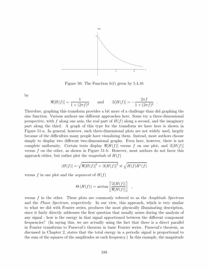
t

h(t)

+1

+2

1

Figure 50: The Function h(t) given by 5.4.16

by

�[H(f)] =1

1 + (2πf)2and �[H(f)] = − 2πf

1 + (2πf)2.

Therefore, graphing this transform provides a bit more of a challenge than did graphing thesinc function. Various authors use different approaches here. Some try a three-dimensionalperspective, with f along one axis, the real part of H(f) along a second, and the imaginarypart along the third. A graph of this type for the transform we have here is shown inFigure 51-a. In general, however, such three-dimensional plots are not widely used, largelybecause of the difficulties many people have visualizing them. Instead, most authors choosesimply to display two different two-dimensional graphs. Even here, however, there is notcomplete uniformity. Certain texts display �[H(f)] versus f on one plot, and �[H(f)]versus f on the other, as shown in Figure 51-b. However, most authors do not favor thisapproach either, but rather plot the magnitude of H(f)

|H(f)| =√�[H(f)]2 + �[H(f)]2 ≡

√H(f)H∗(f)

versus f in one plot and the argument of H(f)

Θ (H(f)) = arctan

[�[H(f)]

�[H(f)]

],

versus f in the other. These plots are commonly referred to as the Amplitude Spectrumand the Phase Spectrum, respectively. In our view, this approach, which is very similarto what we did with Fourier series, produces the most physically illuminating description,since it fairly directly addresses the first question that usually arises during the analysis ofany signal - how is the energy in that signal apportioned between the different componentfrequencies? (In saying this, we are actually using the fact that there is a direct parallelin Fourier transforms to Parseval’s theorem in basic Fourier series. Parseval’s theorem, asdiscussed in Chapter 2, states that the total energy in a periodic signal is proportional tothe sum of the squares of the amplitudes at each frequency.) In this example, the magnitude

188

and argument of H(f) are, respectively

|H(f)| =√H(f)H∗(f) =

1√1 + (2πf)2

and

Θ (H(f)) = arctan

[−2πf

1

]= − arctan [2πf ] .

The graphs of these two quantities are plotted in Figure 51-c. Again, as expected, we seethat the larger amplitudes occur at the lower frequencies. Furthermore, as in the squarepulse, H(f) = O(1/f), a result which again seems reasonable in light of our Fourier seriesexperience, since h(t) is discontinuous at t = 0.

−4 −2 0 2 40

0.5

1

f

ℜ H

(f)

−4 −2 0 2 4−0.5

0

0.5

f

ℑ H

(f)

−4 −2 0 2 40

0.5

1

f

| H(f)

|

−4 −2 0 2 4−2

−1

0

1

2

f

Θ(H

(f))

Figure 51: Alternative Graphical Descriptions of the Fourier Transform

These two examples have introduced some of the basic considerations involved in inter-preting Fourier transforms. We shall continue to use these ideas as we now turn to studythe mechanics of computing these transforms in some more detail.

5.5 Special Computational Cases of the Fourier Transform

Computing Fourier transforms involves, as did computing Fourier series, evaluating inte-grals - an often tedious and time-consuming process. Tables help, but only if the functionyou are looking for is in the tables. In some cases, including developing the tables in the firstplace, one has no choice but to compute the transform by direct integration. Fortunately

189

however, with Fourier transforms, as with the Fourier series, there are certain special caseswhen we can exploit particular properties of h(t) in order to simplify, or even totally avoid,having to fully compute of these integrals. In this section we consider the most importantof these cases - when the time domain function is either even or odd, or when it is zerofor t < 0.

In the case of an even or odd time-domain function, simplification is possible because ofEuler’s identity, and the fact that the integral of a sum is the sum of the integrals. Theseallow us, respectively, to replace the complex exponential in (5.3.13) with trigonometricterms, and then simplify the result as

H(f) =∫ ∞

−∞h(t) cos(2πft)dt− j

∫ ∞

−∞h(t) sin(2πft)dt .

(Note that this formula implies, among other things, that for purely real-valued time domainfunctions (h(t))

�[H(f)] =∫ ∞

−∞h(t) cos(2πft)dt and �[H(f)] = −

∫ ∞

−∞h(t) sin(2πft)dt .

These formulas, unfortunately, are not correct if h(t) is complex.) But, since cos(2πft) iseven and sin(2πft) is odd, then when h(t) is itself real and either even or odd, we cansimplify these integrals, just as we did for the an and bn in the Fourier series. Specifically,by essentially repeating the derivation in Chapter 2, we can show here that

If h(t) is real and even, then

H(f) = 2∫ ∞

0h(t) cos(2πft)dt (5.5.17)

and furthermore H(f) is real and even, and

If h(t) is real and odd, then

H(f) = −2j∫ ∞

0h(t) sin(2πft)dt (5.5.18)

and moreover H(f) is purely imaginary, with an odd imaginary part.

Thus, for example, since the function

h(t) = e−|t|

is clearly even (Figure 52), then according to (5.5.17) we could equally well compute itsFourier transform as

H(f) = 2∫ ∞

0e−t cos(2πft)dt =

2

1 + (2πf)2

(Note however, that in contrast with our two earlier examples, h(t) here is continuous,but h′(t) is not, and therefore, apparently as a consequence of this, H(f) = O(1/f 2).)

190

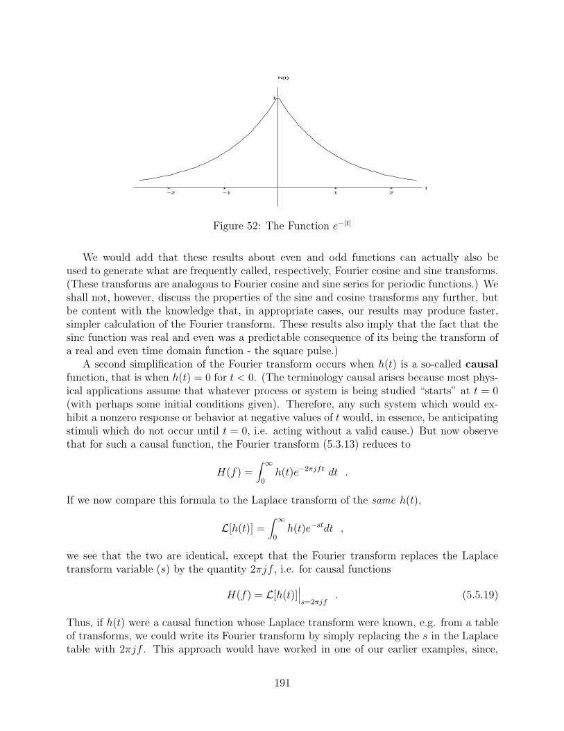
t

h(t)

+1

+2

+−1

+−2

1

Figure 52: The Function e−|t|

We would add that these results about even and odd functions can actually also beused to generate what are frequently called, respectively, Fourier cosine and sine transforms.(These transforms are analogous to Fourier cosine and sine series for periodic functions.) Weshall not, however, discuss the properties of the sine and cosine transforms any further, butbe content with the knowledge that, in appropriate cases, our results may produce faster,simpler calculation of the Fourier transform. These results also imply that the fact that thesinc function was real and even was a predictable consequence of its being the transform ofa real and even time domain function - the square pulse.)

A second simplification of the Fourier transform occurs when h(t) is a so-called causalfunction, that is when h(t) = 0 for t < 0. (The terminology causal arises because most phys-ical applications assume that whatever process or system is being studied “starts” at t = 0(with perhaps some initial conditions given). Therefore, any such system which would ex-hibit a nonzero response or behavior at negative values of t would, in essence, be anticipatingstimuli which do not occur until t = 0, i.e. acting without a valid cause.) But now observethat for such a causal function, the Fourier transform (5.3.13) reduces to

H(f) =∫ ∞

0h(t)e−2πjft dt .

If we now compare this formula to the Laplace transform of the same h(t),

L[h(t)] =∫ ∞

0h(t)e−stdt ,

we see that the two are identical, except that the Fourier transform replaces the Laplacetransform variable (s) by the quantity 2πjf , i.e. for causal functions

H(f) = L[h(t)]∣∣∣s=2πjf

. (5.5.19)

Thus, if h(t) were a causal function whose Laplace transform were known, e.g. from a tableof transforms, we could write its Fourier transform by simply replacing the s in the Laplacetable with 2πjf . This approach would have worked in one of our earlier examples, since,

191

according to standard LaPlace tables

L[e−t] =1

s + 1

and therefore the Fourier transform of the function shown in Figure 50 can be found bysimply letting s = 2πjf , i.e.

H(f) =1

2πjf + 1≡ 1

1 + 2πjf.

(Actually, one needs to be quite careful in applying this result! Specifically, it may produceerroneous results unless the function h(t) is not only causal, but also has a Fourier transformin the “usual” sense, i.e when h(t) satisfies the conditions of Theorem 5.1, e.g. by havingfinite energy. Attempting to apply this method to functions which do not satisfy one of theseconditions may produce incorrect Fourier transforms. One such causal function with infiniteenergy, for which the above procedure does not compute the correct transform, is

h(t) =

{1 , 0 ≤ t0 , otherwise

We shall show how to correctly compute the transform of this function directly, by a differentapproach, in a later section.)

There are more “tricks” which exploit other special properties of h(t) in order to simplifycomputing Fourier transforms, but the above are the principal ones. As with the specialformulas for calculating the Fourier series coefficients of even and odd functions, however, theresults we’ve presented in this section do not really provide any new information which couldnot be obtained by computing the integrals from the standard Fourier transform formula.They only generate what are usually computationally more efficient ways to determine thatinformation in certain special cases.

5.6 Relations Between the Transform and Inverse Transform

Thus far we have defined the Fourier and inverse Fourier integral transforms and computedthe transforms of some example functions. By now, you hopefully also appreciate thatcomputing transforms directly from the definition, i.e. by actually doing the integrationin (5.3.13), is generally not the preferred approach! (After all, who computes derivativesdirectly from their limit definition?) In practice, most Fourier transforms are computedjust as are most Laplace transforms - by using tables, formulas and rules that exploit, asmuch as possible, already computed transforms. In this section, we shall determine certainrelationships between the transform and its inverse that can be used to simplify such Fouriertransform computations.

These relationships depend in part on adopting a view which we have perhaps alreadyalluded to, although not strongly. The central idea of this view is that transforms are, bytheir very nature, functions themselves. The difference is that for a transform, the inputsand outputs are not numbers, but other functions. Thus, in light of our discussion in the

192

first chapter, we could also view the Fourier transform as a “black box,” which inputs time-domain functions and outputs frequency domain ones, i.e.

h(t) −→ F [ ] −→ H(f)

But functions can be equally well specified either analytically (i.e. by a formula) or graph-ically! Therefore, we may equally well think of the Fourier transform as a black box whoseinputs and outputs are graphs. For example, we could view the relationship between thesquare pulse and its Fourier transform as either

{1 , |t| < 1/20 , otherwise

−→ F [ ] −→ sin(πf)

πf

or

t

h(t)

−1+ +

1

1

−→ F [ ] −→ f

H(f)

−1+

−2+

−3+ +

1+2

+3

1

Stated another way, the transform pair is just as completely defined by displaying the re-spective graphs of the time (input) and frequency (output) domain functions as by givingtheir formulas. (Of course, based on our earlier discussion, we might prefer to use multiplegraphs if either the input or output (or both) were complex.)

With this view in mind, we shall now perform a little formal algebra. According to thetransform formulas, any time-domain signal h(t) can be recovered from its frequency-domaintransform H(f) according to the formula

h(t) =∫ ∞

−∞H(f)e2πjftdf

But if, for the moment, we treat the variables t and f as simply symbols, without physicalinterpretation, we can algebraically manipulate them. Specifically, if we replace t by (−f),and f by t, on both sides, we obtain the identity

h(−f) =∫ ∞

−∞H(t)e−2πjftdt (5.6.20)

But look carefully at the right-hand side of this identity and compare it to (5.3.13)! Thisintegral is really nothing more than, by definition, the Fourier transform of the time-domainfunction whose graph is H(t), i.e. the function whose graph has the same shape as a functionof t that H(f) has as a function of f . (For example, in terms of the time-domain squarepulse and its transform, we would have

H(t) =sin(πt)

πt.)

193

Interpreting the left-hand side of (5.6.20) is only slightly more difficult, and this difficultyis due solely to the presence of the minus sign. A little elementary curve sketching shouldconvince you that, for any f , the value on the curve h(−f) is the same as the value onthe curve for h(t) at t = −f . In other words, the curve for h(−f) as a function of f is themirror image (with respect to the vertical axis) of the curve for h(t) - i.e. we simply takethe curve for h(t), swap the positive and negative ends of the horizontal axis, and relabelthe horizontal axis as f (Figure 53). This rather intriguing result can be summarized with

t

h(t)

f

h(−f)

Figure 53: The Relationship of h(t) and h(−f)

the formulaF [H(t)] = h(−f) (5.6.21)

or, in terms of our black boxes,

H(t) −→ F [ ] −→ h(−f)

This result further implies, among other things, that every Fourier transform actually gener-ates two transform pairs, or two entries in any table of transforms. For example, the squarepulse generates both {

1 , |t| < 1/20 , otherwise

←→ sin(πf)

πf

andsin(πt)

πt←→

{1 , |f | < 1/20 , otherwise

(Of course, since h(t) here is an even function, swapping the positive and negative axes toproduce h(−f) produces no perceptible effect.) In terms of our black box model, we couldequivalently portray the result of (5.6.21) for these specific functions as

t

h(t)

−1+ +

1

1

−→ F [ ] −→ f

H(f)

−1+

−2+

−3+ +

1+2

+3

1

and

194

f

H(f)

−1+

−2+

−3+ +

1+2

+3

1

−→ F [ ] −→ t

h(t)

−1+ +

1

1

(We would add that this result has no counterpart in Laplace transform theory.)There is one further interesting result which may be arrived at by manipulating the

Fourier inverse formula

h(t) = F−1 [H(f)] =∫ ∞

−∞H(f)e2πjftdf

If we again algebraically interchange the variables, this time replacing t by f , and f by (−t),we find

h(f) =∫ −∞

∞H(−t)e−2πjft(−dt) ,

or, equivalently,

h(f) =∫ ∞

−∞H(−t)e−2πjftdt . (5.6.22)

If we now compare this integral with the definition of the Fourier transform (5.3.13), we seethat we have here nothing more than the calculation of the Fourier transform of H(−t), i.e.the function whose graph (as a function of t) is the same as the mirror image of the graphof H(f) as a function of f . While at first this may seem to be not all that surprising, itnevertheless has a fundamental practical impact. This impact is very simply that, becauseof (5.6.22), one needs only to design a piece of computer hardware and software that cancalculate the Fourier transform. The identical device can then be used to compute theinverse transform, provided only that one must enter the data in reverse order. The potentialeconomic savings of such an observation are immense.

5.7 General Properties of the Fourier Transform - Linearity, Shift-

ing and Scaling

As we’ve already alluded to, one seldom computes transforms directly from the definition,i.e. by actually integrating (5.3.13). Generally, the preferred approach is to use tables ofalready computed transforms (some of which may have been computed using rules suchas those discussed in the previous section). However, creating and using tables involvescertain tradeoffs - the more complete the table, the longer and more costly it becomes,and the harder it often becomes to find any particular formula. Therefore, any rules orother properties which can cut down on the length of tables, without compromising theireffectiveness are potentially valuable. In this section, we shall develop some common rulesthat can be used to simplify the computation of Fourier transforms, given information aboutthe transforms of related functions.

The first of these rules is a direct and straightforward consequence of the facts that theFourier transform is defined in terms of an integral and that the integral as an operationhas certain properties. Specifically, given two (different) time domain functions, say h(t)

195

and g(t), and constants a and b, then, according to the definition of the transform (5.3.13)and the fact that the integral of a sum is the sum of the integrals

F [ah(t) + bg(t)] =∫ ∞

−∞[ah(t) + bg(t)]e−2πjftdt

= a∫ ∞

−∞h(t)e−2πjftdt+ b

∫ ∞

−∞g(t)e−2πjftdt

= aF [h(t)] + bF [g(t)]

or, equivalentlyF [ah(t) + bg(t)] = aH(f) + bG(f) (5.7.23)

Stated slightly differently, the Fourier transform is a linear operation (as most of the commonoperations of the calculus, such as the derivative and the integral).

The second rule we shall consider involves functions of the form h(at), where h(t) is afunction whose transform, denoted H(f), we already know. (In the following development,we shall assume that a > 0. We invite the reader to ponder what will change when a < 0.)However, in order to be able to better interpret our result, we shall first review, in graphicalterms, the meaning of the expression h(at). Specifically, in terms of our input/output modelof functions, h(at) is the function whose output value, given an input of say t0, is the valueof the original function h(t), but for an input of (at0), not t0. Thus, for an input valueof 1, the function h(at) produces the output value of h(a). This interpretation is depictedin Figure 54, for both the cases a < 1 and a > 1. (Of course, if a = 1, the graphs of h(t)and h(at) are identical.) Note that if a < 1, the graph of h(at) is a spread out version of thegraph of h(t), while if a > 1, it is compressed, i.e. replacing t by at to create h(at) effectivelyrescales the horizontal (t) axis. If we think of t as a physical time variable, then we caninterpret a < 1 as effectively “slowing down” time, while a > 1 “speeds it up.” Viewedanother way, an event that occurs at t = 1 in the function h(t) occurs before t = 1 in thefunction h(at) if a > 1, and after t = 1 if a < 1. A realistic physical model for this situationis a variable speed tape recorder, where a > 1 corresponds to playing the tape faster thanthe speed it was recorded at, and a < 1 to playing it slower.

t1

h(t)

t1

h(at)

a < 1

t1

h(at)

a > 1

Figure 54: The Relationship of h(t) and h(at)

With this model in mind, we now consider the algebra of computing the Fourier transform

196

of h(at). We start at the beginning, with the definition

F [h(at)] =∫ ∞

−∞h(at)e−2πjftdt

If we now change variables inside the integral, replacing t by (t/a), we have

F [h(at)] =∫ ∞

−∞h(t)e−2πjf(t/a)d(t/a)

=1

a

∫ ∞

−∞h(t)e−2πj(f/a)tdt

(Note that this procedure normally also changes the limits on the integral, but because theyare infinite in this case and a is positive, that change will be unnoticeable here.) But acareful look at the last integral here shows that it is, by definition (5.3.13), nothing morethan the Fourier transform of the original, unscaled function h(t), except that this integralis evaluated at f/a, not f . Equivalently, we can now state

F [h(at)] =1

aH

(f

a

)(5.7.24)

Now note the effect of the right hand side of this equality. It is nothing more than a scaledversion of H(f), but with two important distinctions relative to our interpretation of h(at)as a scaled version of h(t). First of all, the vertical scale of H(f/a) is different than thatof H(f), by the factor 1/a. Secondly, the horizontal axis is also scaled by the reciprocal of a.In other words, if a > 1, then in the frequency domain the maximum amplitudes are reduced,and the amplitude spectrum is spread out. Conversely, if a < 1, the maximum amplitudesare both increased and pushed toward the lower frequencies. This behavior is shown inFigure 55. This figure clearly supports common sense, which tells us that when a > 1, theeffect of time scaling on the Fourier transform is to push the energy of h(t) up into thehigher frequencies. In other words, if we try to play our tape recorder in “fast forward,” wewill hear the “Mickey Mouse” sound. The opposite, of course, happens when a < 1. (Don’tforget however that (5.7.24) was derived assuming that a is positive! You should considerhow this result would change if a were negative instead.)

Example: We already have shown that for h(t) = e−|t|

H(f) = F[e−|t|] =

2

1 + (2πf)2

Therefore, according to (5.7.24)

F[e−2|t|

]= 1

2H(

f2

)=

1

2

{2

1 + (2π(f/2))2

}

=1

1 + (πf)2

197

f

H(f)

−1+ +

1

+1

f

H(f)

−1+ +

1

+ 1

a < 1

f

H(f)

−1+ +

1

+1

a > 1

Figure 55: The Relationship of H(f) and1

aH

(f

a

)

A third rule for simplifying the computation of Fourier transforms involves functions ofthe form h(t − b), which are nothing more than identical copies of the function h(t), butshifted to the right (assuming b is positive) by the amount b (Figure 56). Physically, suchshifts generate exactly the same signal, only later in time. To determine the effect of thistime shift on the Fourier transform, we start again with the definition (5.3.13), but thenchange the variables by replacing t by (t+ b) inside the integral. This leads to

F [h(t− b)] =∫ ∞

−∞h(t− b)e−2πjftdt

=∫ ∞

−∞h((t+ b)− b)e−2πjf(t+b)d(t+ b)

= e−2πjfb∫ ∞

−∞h(t)e−2πjftdt .

But, of course, by definition the last integral in the above formula is nothing more than thetransform of the unshifted function. Therefore we can summarize this rule as

F [h(t− b)] = e−2πjfbH(f) (5.7.25)

As was the case with our rule for the transform of a scaled function, this rule also has aclear interpretation in terms of the amplitude and phase spectra in the transform (frequency)domain. Specifically ∣∣∣e−2πjfbH(f)

∣∣∣ =∣∣∣e−2πjfb

∣∣∣ |H(f)| = |H(f)| ,

since∣∣∣e−2πjfb

∣∣∣ = 1, and

Θ(e−2πjfbH(f)

)= Θ

(e−2πjfb

)+ Θ(H(f)) = −2πfb+ Θ(H(f)) .

In other words, a pure time shift introduces absolutely no change in the amplitude spectrum,but only affects the phase. Since a time shift does not really alter the signal (for example,your tape will sound the same tomorrow as it does today, assuming you play it at the samespeed), this result seems perfectly reasonable.

198

tb

h(t)

bt

h(t−b)

Figure 56: The Relationship of h(t) and h(t− b)

Example: Consider the function

g(t) ={

e1−t , 1 < t0 , otherwise

A quick sketch should convince you that this function is nothing more than the function ofFigure 50, shifted to the right by one unit, i.e. g(t) = h(t− 1). Therefore, taking b = 1,

F [g(t)] = e−2πjf(1)H(f) = e−2πjf 1

1 + 2πjf

You may also observe that we can also combine (5.7.24) and (5.7.25) into a single rule,as follows

F [h(at− b)] = F [h(a(t− b/a))] = e−2πjf(b/a)F [h(at)]

=e−2πjf(b/a)

aH

(f

a

) (5.7.26)

The rules and properties presented thus far are by no means exhaustive. However they aresufficient to compute the transforms of many interesting and commonly occurring functions.Equally importantly, they may be used to begin to generate tables of Fourier transforms,in much the same way that tables of Laplace transforms are produced (and then later toextend such tables). Transform tables can significantly streamline and speed up transformcomputations, especially when used in conjunction with linearity, shifting, etc.

5.8 The Fourier Transform of Derivatives and Integrals

The previous section introduced rules which we could use to simplify the computation of theFourier transform of shifted or rescaled versions of a given time-domain function. In thissection we shall develop some further rules that apply to a somewhat different situation -when the function we wish to transform is the derivative or integral of a function whosetransform we know.

You should recall that a very specific relationship exists between the Laplace transformsof a function and its derivative, specifically

L [h′(t)] = sL [h(t)]− h(0) .

199

(Furthermore, this relationship allows us to convert linear, constant coefficient ordinarydifferential equations into algebraic ones which include all the effects of the initial conditions.Unfortunately, as you should also recall, that the resulting algebraic equation is in terms ofthe transform variable, not the original time-domain one. Therefore, we must still invertthe solutions to this algebraic equation in order to recover the solution to the differentialequation.) Given our earlier comments on the similarities between the Fourier and Laplacetransforms, we should not be surprised then if a similar, but perhaps not identical relationoccurs with the Fourier transform.

In the following discussion, as before, we shall denote the particular time-domain functionwhose transform we know by h(t), and its transform byH(f). In addition, we assume that theFourier transform of h′(t) also exists and furthermore that h(t)→ 0 as t→ ±∞. (This lastrestriction is actually less of an assumption that an almost virtually guaranteed consequenceif h(t) is any function which satisfies Theorem 5.1.) With these assumptions, we start withthe definition of the transform and integrate by parts one time, to yield

F [h′(t)] =∫ ∞

−∞h′(t)e−2πjftdt

= h(t)e−2πjft

∣∣∣∣∣∞

−∞−∫ ∞

−∞h(t)

[−(2πjf)e−2πjft

]dt

= h(t)e−2πjft

∣∣∣∣∣∞

−∞+ 2πjf

∫ ∞

−∞h(t)e−2πjftdt

But since, by assumption, h(t) vanishes at ±∞, the first term in the last equation drops out.Moreover, the integral in the second term is, by definition, nothing more than the Fouriertransform of the original, undifferentiated time-domain function. Therefore, we have shown

F [h′(t)] = 2πjfH(f) (5.8.27)

Note that, hopefully not unexpectedly, this is very similar to the result for the Laplacetransform of the derivative. The major difference, outside of the replacement of the Laplacevariable (s) by the Fourier term (2πjf), is that no initial value data appears in the Fouriertransform of the derivative. On reflection however, this lack of initial data in the Fouriertransform should not seem all that surprising. After all, the Laplace transform only integratesvalues for t > 0. Therefore, in line with the basic theory of ordinary differential equations,some initial data would seem to be mandatory when transforming the derivative. On thecontrary, the Fourier transform should not need initial data, since its interval of integrationassumes the values of the function are known “for all time.”

Later we shall see how (5.8.27) can be used in the solution of differential equations. Forthe moment however, we consider it as just another rule that may be invoked, if required,to simplify the computations. Thus consider the following

Example: While we could compute the Fourier transform of the function

g(t) ={ − e−t , 0 ≤ t <∞

et , −∞ < t < 0

200

t

h(t)

+1

+−1

1

−1

f

|H(f)|

+1

+−1

1

Figure 57: A Fourier Transform Computed Using the Derivative Rule

(Figure 57) directly (and simplify that computation by using the fact that g(t) is an oddfunction), note that

g(t) =d

dt

[e−|t|] .

Since we have already computed the Fourier transform of e−|t|, we can thus use that earliercomputation, plus this last rule to state

F [g(t)] = F[

ddt

[e−|t|

]]= 2πjfF

[e−|t|]

= 2πjf

{2

1 + (2πf)2

}=

4πjf

1 + (2πf)2

(Again, as we already observed, the time-domain function g(t) here was odd. Therefore, aswe should have expected, based on our earlier discussion, this transform is purely imaginaryand the imaginary part itself is an odd function. Furthermore, the transform is O(1/f)as f→ ±∞, apparently as a consequence of the jump in g(t) at t = 0.)

Finally, you should note that we can apply (5.8.27) repeatedly, as we commonly do withthe corresponding rule for Laplace transforms, and show that

F[dnh

dtn

]= (2πjf)nH(f) (5.8.28)

Derivatives also figure prominently in the next Fourier transform rule we consider, butfrom a different perspective. Specifically, the transform H(f) is itself a function of f . There-fore, it seems reasonable to see if there is any valuable information in the derivative of H(f)with respect to f . To determine this, we again start with the definition of the transform,

201

then apply the usual Liebnitz rule for differentiating under an integral sign

d

df[H(f)] ≡ d

df

[∫ ∞

−∞h(t)e−2πjftdt

]

=∫ ∞

−∞∂

∂f

[h(t)e−2πjft

]dt

=∫ ∞

−∞h(t)

[−2πjte−2πjft

]dt

= −2πj∫ ∞

−∞[th(t)] e−2πjftdt

But this last integral is simply by definition the Fourier transform of the quantity [th(t)].Therefore, after dividing both sides by the (−2πj) factor, we have

F [th(t)] = − 1

2πj

d

df[H(f)] (5.8.29)

or, when applied repeatedly

F [tnh(t)] =(−1)n

(2πj)n

dn

dfn[H(f)] (5.8.30)

(where, of course, for this to be valid, tnh(t) must also satisfy the conditions of Theorem 5.1).The use of this rule is demonstrated by the following

Example: Considerg(t) = te−|t| , −∞ < t <∞

Now, according to our last result, since we already have computed the Fourier transformof e−|t|,

G(f) = F[te−|t|

]= − 1

2πj

d

df

[F[e−|t|]]

= − 1

2πj

d

df

[2

1 + (2πf)2

]=

−8πjf

(1 + (2πf)2)2

(Again note how the oddness of g(t) evidences itself in G(f) being purely imaginary with anodd imaginary part, and the fact that H(f) = O(1/f 3) relates to the fact that h(t) and h′(t)here are both continuous.)

The last rule we shall consider in this section is basically the reverse of the derivativerule. Specifically, from the fundamental theorem of the integral calculus,

h(t) =d

dt

[∫ t

−∞h(s)ds

]

and therefore, by (5.8.27)

H(f) = F [h(t)] = 2πjf F[∫ t

−∞h(s)ds

]

202

or equivalently

F[∫ t

−∞h(s)ds

]=H(f)

2πjf, (5.8.31)

provided that∫ ∞

−∞h(t)dt = 0 (This last restriction is necessary in order to satisfy our earlier

requirement that any function whose derivative we are transforming must vanish at ±∞.)This section completes the first part of our introduction to definition, interpretation and

computation of the Fourier transform. We could perhaps continue and derive a few otherrules, but the ones we have covered so far represent the principal ones needed to compute thetransform of “normal” functions, i.e. those that satisfy one of the two tests of Theorem 5.1.Unfortunately, many real-world applications involve signals that are most easily modeledby functions that do not satisfy this theorem. (The periodic functions are one obviousexample.) Therefore, rather than continue to try to find more rules for normal functions,we shall turn instead in the next section to extending the definition and computation of theFourier transform to a broader class of physically interesting functions.

5.9 The Fourier Transform of the Impulse Function and Its Im-plications

We have already briefly mentioned the impulse or delta function, which we assume youhave already been introduced to in Laplace transforms. This function (which is really nota function in the sense of the usual calculus) is normally symbolized by δ(t) and representsan “instantaneous” force, such as occurs in the inelastic collision between billiard balls. (Ofcourse, no truly instantaneous forces exist, just as there are no truly periodic ones. Whatthere are, however, are forces which act over such short periods of time, relative to thetime scales of the rest of a particular physical process, that they appear to be effectivelyinstantaneous in that process.) However, instantaneous forces create a minor mathematicaldilemma. The reason is that a force, to be instantaneous, must be zero at all times other thanthe instant of application. But, mathematically, a force also produces no noticeable effectunless it accomplishes physical work, and work is related to the integral of the magnitude ofthe force over its duration of application. Therefore, since in the usual calculus sense the areaunder a point of finite height is zero, a force of finite amplitude and instantaneous durationcan do no physical work. Hence, to have any physical effect, an instantaneous force must bemodeled as having an infinite amplitude at the instant of application. Such functions clearlycannot be treated by the normal calculus.

Physically, a model instantaneous force is completely determined once we know when itoccurs and the value of its integral . (This integral, which we will colloquially refer to as thearea under the instantaneous function, of course effectively determines the amount of workthe force can perform.) Thus, the simplest instantaneous force to consider would seem toone acting at t = 0 and with unit area - this, of course, becomes what we call δ(t), or the unitimpulse. Most texts usually generate δ(t) as the limit of a set of even rectangular pulses ofunit area and continually smaller duration (and hence proportionally growing amplitudes).As their limit, δ(t) will thus have infinite amplitude at t = 0 and be zero elsewhere. Graph-ically, it is usually portrayed as a bold-face vertical arrow, or “spike” of unit height located

203

at t = 0 (Figure 58). In line with the above discussion, its basic properties are usually statedas

δ(t) = 0 , t = 0and ∫∞

−∞ δ(t− t0) dt = 1

t

p/2−p/2

1/p

∆p(t)

−−−−−−−−−−−−>

as p −> 0

t

δ(t)

1

Figure 58: The Graphical Interpretations of δ(t)

Of course, not all instantaneous forces need occur at t = 0. Therefore, we must also be ableto represent an instantaneous force of unit area and located at some t = t0 = 0. Notationally,we do this in the “natural” way, i.e. with the symbol δ(t− t0). In terms of this notation, wecan then show that the delta function also satisfies a third critical equality, commonly calledthe sifting property. The sifting property states that, for any continuous function h(t),∫ ∞

−∞h(t)δ(t− t0) dt = h(t0) .

(Note that while we mentally view δ(t− t0) as an infinitely strong pulse of unit area locatedat t = t0, we shall graphically portray it as simply a shifted copy of δ(t), i.e. as a bold spikeof unit height at t = t0.) Furthermore, since the sifting property implies that∫ ∞

−∞cδ(t− t0) dt = c ,

where c is any constant, we shall therefore graph an instantaneous force with area (work) cwhich occurs at t = t0 as a spike of height c located at t0. Moreover, since the area of theunit impulse does not change, we can easily adopt the view that its location coincides withthe point where the overall argument (e.g. t− t0) is zero, and state the following equalities

δ(t0 − t) = δ(t− t0)δ(−t) = δ(t)

(Alternatively, according to this last equation, we may say that Figure 58 implies that thedelta function is even.) Finally, since Figure 58 seems clearly to allow us to consider theimpulse as a real and non-negative valued function, we shall also accept

|δ(t)| = δ(t)

204

Before continuing, we must reemphasize that, because of its infinite height, the deltafunction is not a function in the sense of the ordinary calculus. Moreover, not all of itsproperties are intuitively clear. (For example, as we will show later

δ(2t) =1

2δ(t) ,

a result which seems, at face value, to be inconsistent with the graphical interpretation ofthe time scaling of “normal” functions as portrayed in Figure 54.) Therefore, any mathe-matics involving the delta function must really be justified by arguments beyond those ofthe ordinary calculus, e.g. the sifting property cannot really be justified in terms of nor-mal integrals. Such justifications do exist, and form the core of a rather elegant section ofmathematics called distribution or generalized function theory. This theory is, however, wellbeyond our level. Therefore much of the following development will be formal rather thanrigorous. Fortunately, we can formally derive all of the results using little more than thesifting property and the concept of the Fourier transform as a pair.

We start by considering the Fourier transform of the shifted delta function. Assumingthat this transform actually exists, we can then compute it formally from the definition ofthe transform and the sifting property as

F [δ(t− t0)] ≡∫ ∞

−∞δ(t− t0)e−2πjftdt = e−2πjft0

Furthermore, if we then evaluate this transform at t0 = 0, we have the second transform pair

F [δ(t)] = 1

(Figure 59). But according to the symmetry property of the transform, i.e. the propertythat F [H(t)] = h(−f), we immediately have still another transform pair

t

δ(t)

1+

f

H(f)

Figure 59: The Transform Pair for F [δ(t)] = 1

F [1] = δ(−f) = δ(f)

(where we now apply our earlier view of the delta function as even.) This pair immediatelyleads to a fairly powerful insight on the nature of the transform. A physical model for theconstant function in the time domain is a direct current (DC) battery that never runs down.

205

(Such a battery is, of course, unrealizable since it must store infinite energy.) But recall theFourier transform supposedly identifies the amplitudes of the component frequencies of atime-domain signal! Therefore, it seems quite reasonable that the transform of the constantfunction should be a delta function located at the origin in the frequency domain. Its “real”height is infinite, because, of course, the battery apparently has infinite energy, while itsarea (as denoted by the height of the spike) corresponds exactly to the amplitude of the timedomain signal. The location of the spike also seems appropriate, since by definition directcurrent does not oscillate.

The symmetry property of the transform and the fact that the unit impulse is uniquelycharacterized by the location of the zero of its argument also allow us to compute anothernew pair

F[e−2πjf0t

]= δ(−f − f0) = δ(f + f0) .

This particular pair, however, is not very illuminating in and of itself, since complex-valuedtime-domain signals are somewhat unrealistic. However, we can use it to compute severalmore relevant transforms. The first of these uses this transform, along with the identity,

cos(t) =ejt + e−jt

2

and the linearity of the transform, as follows:

F [cos(2πf0t)] = F[1

2e2πjf0t +

1

2e−2πjf0t

]

=1

2F[e2πjf0t

]+

1

2F[e−2πjf0t

]

=1

2δ(f − f0) +

1

2δ(f + f0)

This result yields still another fairly valuable insight into the general nature of the transform.The cosine represents a single pure frequency (f0) in the time domain, which, because it isperiodic, also contains an infinite amount of energy. Its transform consists of exactly twofrequency domain impulses, located at (±f0), i.e. at precisely the frequency (and its negative)of the time domain oscillation. These impulses apparently have a similar interpretation tothe impulse at the origin for the direct current battery, i.e. they connote infinite energy inthe time domain exists at the real frequency f0. Furthermore, each of these impulses hasan area exactly half the amplitude of the real time-domain periodic function. This againis behavior we have previously encountered, for the complex Fourier series also divides theamplitudes of a real signal evenly between the positive and negative frequencies in frequencydomain.

Using essentially the same steps as we used above, we can also show that

F [sin(2πf0t)] =j

2δ(f + f0)− j

2δ(f − f0) ,

206

t

cos(2 pi f0 t)

1+

−1+

++

−1/f0 1/f

0

f

H(f)1

−f0 f

0

Figure 60: The Transform Pair for F [cos(2πf0t)]

t

sin(2 pi f0 t)

1+

−1+

++−1/f

0 1/f0

f

Im(H(f))1

−1

−f0

f0

Figure 61: The Transform Pair for F [sin(2πf0t)]

and, except for the fact that this transform is purely imaginary (apparently a direct conse-quence of the oddness of the sine function), make similar conclusions that were made aboutthe transform of the cosine (Figure 60).

The transform of the complex exponential provides at least one additional interestinginsight. We have already seen that a general periodic function (h(t)) in the time domain canalways be represented in the complex Fourier series form

h(t) =∞∑

n=−∞cne

2jnπf0t ,

where, in terms of our earlier notation f0 = 1/(2L). Therefore, provided we assume that thelinearity of the Fourier transform applies to the sum of convergent infinite series as well asto the sum of just two terms (a very non-trivial assumption), we have, formally,

F [h(t)] =∞∑

n=−∞cnδ(f − nf0) .

In other words, the transform of a general periodic function is an infinite “train” of impulses,located at all multiples of the fundamental frequency (plus of course the constant (DC) term).Each impulse has an area equal to (i.e. is drawn graphically as a spike with an amplitudeof) the value of the corresponding complex Fourier series coefficient. Thus, except for theinclusion of the “arrowheads” to signify impulses, the graph of |H(f)| for this transformwould look identical to the amplitude spectrum for the original Fourier series, as developedin Chapter 2.

207

t−2 −1 21

h(t)

1

f−2 2

.5

|H(f)|

Figure 62: The Transform Pair for a Periodic Function

We close this section with one last insight about impulses. Somewhat in contrast to theones thus far, this one highlights one important difference between “normal” functions andimpulses - the effect of time scaling. Consider δ(2t) . According to our earlier discussions,this is still clearly an impulse and is located at t = 0. But is it still a unit (i.e. unit area)impulse? Interesting enough, if we assume that impulses obey the basic “rules” derived thusfar for Fourier transforms, it is not! Specifically, according to (5.7.24), with a = 2,

F [δ(2t)] =1

2F [δ(t)]

∣∣∣ f2

=1

2[ 1 ]

∣∣∣ f2

=1

2=

1

2F [δ(t)] = F

[1

2δ(t)

]

Thus, we must conclude that exactly one of the following is true

• δ(2t) =1

2δ(t) ,

• Time-domain impulses and their transforms cannot be considered as inseparable pairs,or

• Impulses do not satisfy all the rules for Fourier transforms.

Since the last two choices are very unattractive, we must basically accept the first one, i.e.define

δ(2t) =1

2δ(t)

(Actually, this is not really a very painful choice to have to make. Furthermore, this is theonly interpretation that is consistent with the “natural” view that δ(2t) should be the limit,as p→ 0, of the square pulses given by ∆p(2t), where ∆p(t) is defined in Figure 58.)

This completes our introduction to the relationships between impulses and Fourier trans-forms. Most of the insights developed here should be physically quite satisfying. Moreover,because some of these results seem to imply that one can meaningfully talk about the trans-forms of at least some time-domain functions which represent an infinite amount of energy,we shall next try to extend the notion of the transform to other, non-periodic, functions withinfinite energy.

208

5.10 Further Extensions of the Fourier Transform

In previous sections we have developed the Fourier transform and its properties for both“normal” functions (i.e. those that satisfy one of the two tests of Theorem 5.1), and im-pulses and periodic functions. The fact that we can extend the transform to the periodicfunctions strongly implies that, if we are willing to accept impulses or other singularities inthe transform domain, we may extend the transform even further to include other infiniteenergy functions. This is in fact the case, although any rigorous showing of this would requireconcepts for distribution theory that are well beyond the level of this text. Therefore, as withother similar properties, we shall proceed in a rather formal manner. Our basic approachhowever will be fairly intuitive in that we shall start by trying to approximate such functionswith other functions that are “close” in some sense, but also have Fourier transforms in thenormal sense.

Throughout the following discussion, we will assume that two restrictions hold true

1. h(t) is bounded, i.e. |h(t)| < M for some constant M and all values of t, and

2. h(t) contains no periodic components

Under these restrictions, we now proceed to consider the transforms of two special cases offunctions which do not satisfy Theorem 5.1. The first of these is

Case I: limL→∞

[1

2L

∫ L

−Lh(t)dt

]= 0

In terms of electric circuits, Case I functions can be interpreted physically as having nolong-term average DC level. We shall define the Fourier transform of such functions to be

H(f) = limα→0+

[∫ ∞

−∞

{e−α|t|h(t)

}e−2πjftdt

](5.10.32)

provided such a limit exists. (If no such limit were to exist, we would assume that the functiondid not have a transform.) Observe carefully what we have in effect done here. Physically,we claim it seems to be the most reasonable thing to do. First of all, since we have assumedthat the function h(t) is bounded, then multiplying it by the decaying exponential e−α|t|

produces an integrand which clearly satisfies the conditions of Theorem 5.1, for all α > 0.Thus the transform of h(t)e−α|t| should be a perfectly “well-behaved” function for all α > 0,and therefore we should be able to formally take the limit as α→ 0+ fairly easily. However,for “small” values of α (i.e. for very weak decay), h(t) and h(t)e−α|t| should be reasonablyclose to each other, at least for a fairly “long” period of time. Furthermore, the smaller αbecomes, the closer h(t) and h(t)e−α|t| should become. Therefore, it seems very plausiblethat, as α decreases their transforms should also become closer, and, in the limit as α→ 0+,become identical. (We would again note however, that in dealing with improper integrals,which include the Fourier transform, as in dealing with infinite series, plausible results arenot always correct - witness Zeno’s paradox. Therefore we strongly advise the reader who

209

may need to extend these results beyond the examples presented here to first consult a textwhich contains a more complete discussion of generalized functions and their transforms.)

Computing the transform of a Case I type function is illustrated by the following

Example:

sgn(t) =

⎧⎨⎩

1 , 0 < t <∞0 , t = 0− 1 , −∞ < t < 0

(Figure 63). This function, which really represents nothing more than the algebraic sign

t−1 1

h(t)

1

−1

f−2 2

.5

|H(f)|

Figure 63: The Transform Pair for the Function sgn(t)

of t, clearly does not satisfy the conditions of Theorem 5.1, but does satisfy the conditions ofCase I. Therefore, using the fact that sgn(t) is obviously odd, we may compute its transformaccording to the above procedure as follows

F [sgn(t)] = limα→0+

F[e−α|t|sgn(t)

]

= limα→0+

[∫ ∞

−∞

{e−α|t|sgn(t)

}e−2πjftdt

]

= −2j limα→0+

[∫ ∞

0e−αt sin(2πft)dt

]

= −2j limα→0+

[2πf

α2 + (2πf)2

]= − j

πf

Note that, hopefully not unexpectedly, this transform is singular at the origin.Functions which do not satisfy the restriction of Case I, but do satisfy the other restric-

tions of this section will be called Case II type functions. Specifically, Case II functions occurwhen

Case II: limL→∞

[1

2L

∫ L

−Lh(t)dt

]= A = 0 (In line with our earlier discussion,

we shall then interpret Case II functions as those which, in the electrical sense, have along-term average DC level. Note that, based on our earlier discussion of the impulses, wenow clearly expect the transforms of such functions, if they can be computed, to have an

210

impulse at the origin in the frequency domain.) We treat Case II functions by a standardmathematical ploy - reducing them to a problem we’ve already solved. Specifically, if h(t) isany Case II function, then we can write

h(t) = A+ g(t)

(Graphically, g(t) is simply h(t) shifted down by the amount A, i.e. it’s h(t) but with the DClevel removed.) But as we have already discussed, the Fourier transform is a linear operationand therefore we have

F [h(t)] = F [A] + F [g(t)] = Aδ(f) + F [g(t)]

However, g(t) as constructed is clearly a Case I type function, since all of the long-term DClevel in h(t) is contained in A. Therefore, if we don’t already know the transform of g(t), wecan compute it by the procedure we just finished describing for Case I functions. Thus thetransform of h(t) is completely determined.

Example: Consider the function commonly called the unit step (Figure 64).

u(t) ={

1 , 0 ≤ t <∞0 , −∞ < t < 0

It’s quite easy to show that this function has a long-term average DC level of 1/2, and

t−1 1

h(t)

1

f−2 −1 1 2

1

|H(f)|

Figure 64: The Transform Pair for the Unit Step Function

therefore, based on the immediately previous discussion, we shall represent it as

u(t) =1

2+

1

2sgn(t)

But now, also according to that discussion, and the transform example computed just beforethis one, we have

F [u(t)] = F[

12

+ 12

sgn(t)]

= 12F [1] + 1

2F [sgn(t)]

=1

2δ(f)− j

2πf

(Note the presence of the expected impulse at the origin with a height equal to the DC levelin the time domain. This pattern by now should be expected. Note also that even though

211

the time domain function in this example is causal and Laplace transformable, we wouldobtain an erroneous result, missing the impulse at the origin, if we simply replaced the s inits Laplace transform by 2πjf . This is why we cautioned you earlier about converting theLaplace transforms of functions that did not satisfy the conditions of Theorem 5.1.)

This last example completes our discussion of the transform of functions with infiniteenergy. While there are undoubtedly more rules and properties associated with comput-ing the transform which we could study, we hope you appreciate that our interest in thistransform is not primarily as a formula to be evaluated. On the contrary, our interest inthis transform, as in any transform, is primarily in its utility as a tool which we can use tosolve physical problems. Therefore, in the next chapter, we turn to investigating some of thevarious problems to which the Fourier transform may be applied, and consider some of theinsights into physical processes that it and its dual time-domain/frequency-domain view ofthe world provide.

212

PROBLEMS

1. Compute, from the definition, and using the properties of even and odd functionswhere appropriate, the Fourier transform of each of the following functions. In each case,plot h(t) and the Amplitude spectrum and phase angle graphs.

a. h(t) = e−α|t| , −∞ < t <∞ , α > 0.

(Plot for α = 1 and α = .05)

b. h(t) ={

1 , 0 ≤ t ≤ 10 , otherwise

c. h(t) ={te−t , 0 < t <∞

0 , otherwise

d. h(t) ={

(1− t2) , −1 < t < 10 , otherwise

e. h(t) ={

(1− t)2 , −1 < t < 10 , otherwise

f. h(t) = Ae−α|t| cos(2πt) , −∞ < t <∞ , α > 0 .

(Plot for α = 1 and α = .05)

g. h(t) =

⎧⎪⎪⎪⎨⎪⎪⎪⎩

(1 + t) , −1 < t < 01 , 0 ≤ t ≤ 1

(2− t) , 1 < t < 20 , otherwise

h. h(t) = Ate−α|t| , −∞ < t <∞ , α > 0

i. h(t) ={

t , −1 < t < 10 , otherwise

2. Find, directly from the definition, the inverse of the following Fourier transforms, andplot h(t) and the amplitude and phase graphs:

a. H(f) ={

(1− f 2)2 , −1 < f < 10 , otherwise

b. H(f) = |f | e−2|f | , −∞ < f <∞ .

213

PROBLEMS1. Compute the Fourier transform of each of the following functions, using tables, shiftingand scaling, etc. when appropriate. In each case, plot h(t) and the Amplitude spectrum andphase angle graphs.

a. h(t) ={

2 , −1 < t < 50 , otherwise

b. h(t) =

⎧⎨⎩

t , 0 ≤ t ≤ 24− t , 2 < t ≤ 4

0 , otherwise

c. h(t) = sin(t

3

)

d. h(t) ={

2 , 3 < t <∞0 , otherwise

e. h(t) =1

4 + t2

f. h(t) =sin2(3t)

6t2

g. h(t) ={e−t , 0 < t < 2

0 , otherwise

2. Find, using tables, shifting and/or scaling, etc., the inverse of each of the following Fouriertransforms, and plot h(t) and the amplitude and phase graphs:

a. H(f) =1

1 + f 2, −∞ < f <∞

b. H(f) = e−3jπfe−2|f | , −∞ < f <∞

c. H(f) ={

2 , −3 < f < 30 , otherwise

214

6 Applications of the Fourier Transform

6.1 Introduction

The Fourier transform has become widely used as a tool in mathematics, physics and en-gineering - especially in the solution of differential equations and in the design of signalprocessing systems. We have already encountered some of the properties that have made itso popular - its linearity, the manner in which it relates the transform of a derivative to thetransform of the original function, and its ability to describe the behavior of systems on afrequency-by-frequency basis.

In this chapter we shall briefly examine some of the more commonly found applicationsof the Fourier transform. Our intent is neither to be all-inclusive nor to conduct in-depthengineering analyses. On the contrary, we simply want to show, in the context of some ofits more classic applications, how the Fourier transform is used and how it helps to provideunique and powerful insights into the behavior of physical systems.

However, before we can do this we must develop one more property of the transform. Thisproperty involves the operation called convolution, and may be the transform’s single mostimportant one in relation to the applications we will consider. In one sense, the behavior ofthe Fourier transform relative to convolution may be viewed as simply one more rule, likethose of the previous chapter. However, convolution is so central to applications that wechose not to present it earlier, but instead waited to consider it in this chapter. (There isactually also a second operation, called correlation, which is perhaps almost as importantin other applications as is the convolution. We shall briefly note its properties in relation toFourier transforms at the end of this chapter.)

6.2 Convolution and Fourier Transforms

We define the convolution of two functions, say h(t) and g(t) as

g(t) ∗ h(t) =∫ ∞

−∞g(τ)h(t− τ)dτ . (6.2.1)

The order in which we write g(t) and h(t) here is actually irrelevant, since it is fairly easilyshown that ∫ ∞

−∞g(t− τ)h(τ)dτ =

∫ ∞

−∞g(τ)h(t− τ)dτ

and thereforeg(t) ∗ h(t) ≡ h(t) ∗ g(t) ,

i.e. convolution is a commutative operation. It is, however, crucial to recognize that whilethe variable τ in (6.2.1) is a dummy variable, the variable t is not! Therefore the convolutionof two functions is itself a function, i.e. h(t) ∗ g(t) is a graph, not a number!

You should have already encountered the term convolution in your study of Laplacetransforms. If so, parts of the above definition should seem familiar. But (6.2.1) is notidentical to the definition of convolution for Laplace transform functions, since the lower

215

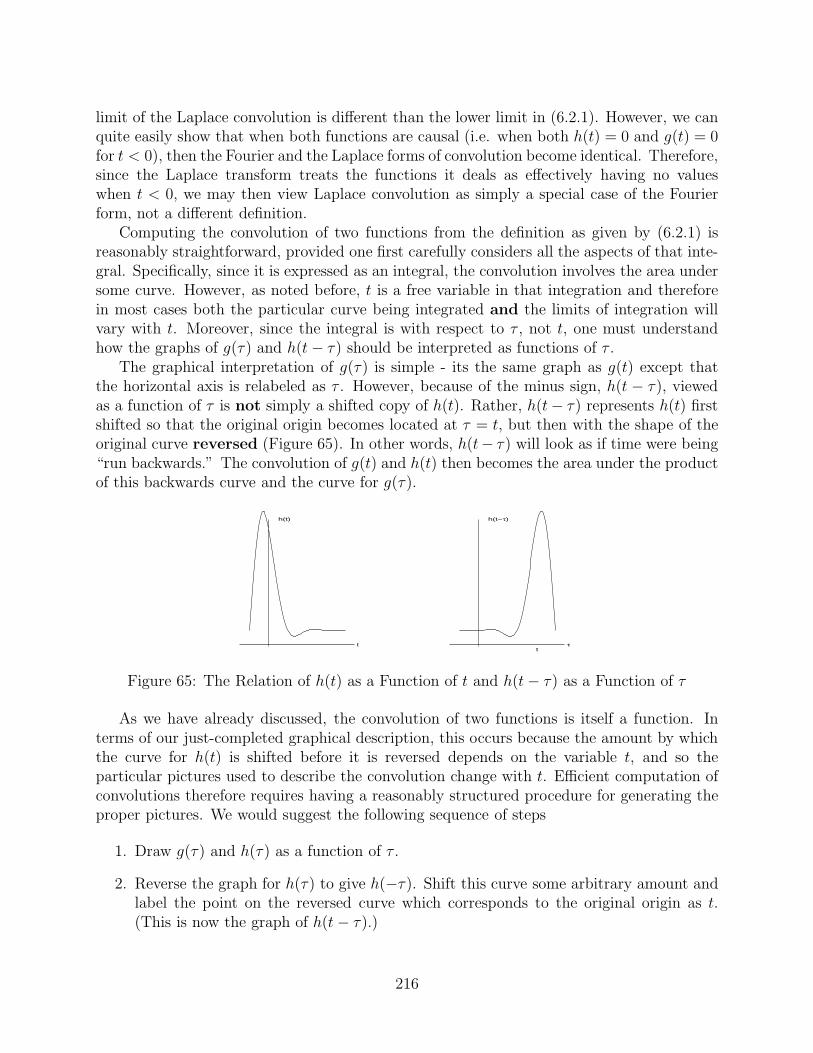
limit of the Laplace convolution is different than the lower limit in (6.2.1). However, we canquite easily show that when both functions are causal (i.e. when both h(t) = 0 and g(t) = 0for t < 0), then the Fourier and the Laplace forms of convolution become identical. Therefore,since the Laplace transform treats the functions it deals as effectively having no valueswhen t < 0, we may then view Laplace convolution as simply a special case of the Fourierform, not a different definition.

Computing the convolution of two functions from the definition as given by (6.2.1) isreasonably straightforward, provided one first carefully considers all the aspects of that inte-gral. Specifically, since it is expressed as an integral, the convolution involves the area undersome curve. However, as noted before, t is a free variable in that integration and thereforein most cases both the particular curve being integrated and the limits of integration willvary with t. Moreover, since the integral is with respect to τ , not t, one must understandhow the graphs of g(τ) and h(t− τ) should be interpreted as functions of τ .

The graphical interpretation of g(τ) is simple - its the same graph as g(t) except thatthe horizontal axis is relabeled as τ . However, because of the minus sign, h(t − τ), viewedas a function of τ is not simply a shifted copy of h(t). Rather, h(t− τ) represents h(t) firstshifted so that the original origin becomes located at τ = t, but then with the shape of theoriginal curve reversed (Figure 65). In other words, h(t− τ) will look as if time were being“run backwards.” The convolution of g(t) and h(t) then becomes the area under the productof this backwards curve and the curve for g(τ).

t

h(t)

τ

h(t−τ)

t

Figure 65: The Relation of h(t) as a Function of t and h(t− τ) as a Function of τ

As we have already discussed, the convolution of two functions is itself a function. Interms of our just-completed graphical description, this occurs because the amount by whichthe curve for h(t) is shifted before it is reversed depends on the variable t, and so theparticular pictures used to describe the convolution change with t. Efficient computation ofconvolutions therefore requires having a reasonably structured procedure for generating theproper pictures. We would suggest the following sequence of steps

1. Draw g(τ) and h(τ) as a function of τ .

2. Reverse the graph for h(τ) to give h(−τ). Shift this curve some arbitrary amount andlabel the point on the reversed curve which corresponds to the original origin as t.(This is now the graph of h(t− τ).)

216

3. Lay the graph for h(t−τ) on top of that for g(τ), with the point labeled with t locatednear τ = −∞ on the graph for g(τ).

4. Slowly slide the graph for h(t − τ) to the right. At any point, the area under theproduct of the two graphs is the convolution for that value of t.

To demonstrate this procedure, consider the following

Example:

g(t) ={

1 , 0 < t < 10 , otherwise

h(t) ={

e−t , 0 ≤ t <∞0 , −∞ < t < 0

(Figure 66) Notice that after we apply the second step, we can think of the reversed ex-ponential as having a “leading edge” at τ = t. Therefore, initially (when t < 0) it has nononzero values in common with the square pulse, and so their product (and the integrandfor the convolution) would be zero (Case I). Eventually, however, as the leading edge of thereversed exponential moves further to the right, it begins to intersect the pulse, causing anonzero integrand between the origin and the point τ = t (Case II). Finally, the leading edgeof the reversed exponential will move to the right of the leading edge of the pulse and therewill be a nonzero integrand only between the origin and τ = 1 (Case III). Computationally,we can express these three cases as

Case I : −∞ < t ≤ 0 ,g(t) ∗ h(t) = 0

Case II : 0 < t < 1 ,

g(t) ∗ h(t) =∫ t

01 · e−(t−τ) dτ = e−(t−τ)

∣∣∣t0

= 1− e−t

Case III : 1 ≤ t <∞ ,

g(t) ∗ h(t) =∫ 1

01 · e−(t−τ) dτ = e−(t−τ)

∣∣∣10

= e−(t−1) − e−t

Lastly, we can combine these three cases into a single graph (Figure 67) which representsthe convolution of these two functions.

Now, with hopefully a firm(er) understanding of the mechanics of computing convolu-tions, we consider how the Fourier transform of a convolution relates to the Fourier trans-forms of the two individual functions which produced that convolution. We start by assumingthat g(t) and h(t) both have transforms, which we denote respectively as G(f) and H(f).Then, as we have in most previous discussions, we write the formal definition for the trans-form of their convolution, i.e.

F [g(t) ∗ h(t)] =∫ ∞

−∞

{∫ ∞

−∞g(τ)h(t− τ)dτ

}e−2πjftdt .

217

t−3 3

g(t)1

t−3 3

1h(t)

τ−3 3

g(τ)1

τ−3 3

1

t

h(t−τ)

τt−3 3

1h(t−τ)

Case I

t < 0

τt−3 3

1h(t−τ)

Case II

0 < t < 1

τt−3 3

1h(t−τ) Case III

t > 1

Figure 66: The Graphical Description of a Convolution

However, since this is now a double integral, we may at least formally interchange the orderof integration and write

F [g(t) ∗ h(t)] =∫ ∞

−∞

{∫ ∞

−∞g(τ)h(t− τ)e−2πjftdt

}dτ

(Note, as in most of our other discussions of the Fourier transform, we call this interchangeformal because we really have not rigorously justified extending the basic calculus resultto improper integrals such as these.) But, with the integral now written this way, we maymove g(τ) outside of the new inner integral, since it does not depend on the variable ofintegration (t) there. This yields

F [g(t) ∗ h(t)] =∫ ∞

−∞g(τ)

{∫ ∞

−∞h(t− τ)e−2πjftdt

}dτ

218

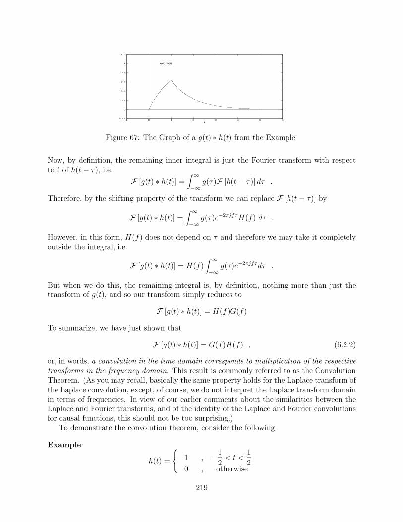
−1 0 1 2 3 4 5 6−0.2

0

0.2

0.4

0.6

0.8

1

1.2

g(t)*h(t)

t

Figure 67: The Graph of a g(t) ∗ h(t) from the Example

Now, by definition, the remaining inner integral is just the Fourier transform with respectto t of h(t− τ), i.e.

F [g(t) ∗ h(t)] =∫ ∞

−∞g(τ)F [h(t− τ)] dτ .

Therefore, by the shifting property of the transform we can replace F [h(t− τ)] by

F [g(t) ∗ h(t)] =∫ ∞

−∞g(τ)e−2πjfτH(f) dτ .

However, in this form, H(f) does not depend on τ and therefore we may take it completelyoutside the integral, i.e.

F [g(t) ∗ h(t)] = H(f)∫ ∞

−∞g(τ)e−2πjfτdτ .

But when we do this, the remaining integral is, by definition, nothing more than just thetransform of g(t), and so our transform simply reduces to

F [g(t) ∗ h(t)] = H(f)G(f)

To summarize, we have just shown that

F [g(t) ∗ h(t)] = G(f)H(f) , (6.2.2)

or, in words, a convolution in the time domain corresponds to multiplication of the respectivetransforms in the frequency domain. This result is commonly referred to as the ConvolutionTheorem. (As you may recall, basically the same property holds for the Laplace transform ofthe Laplace convolution, except, of course, we do not interpret the Laplace transform domainin terms of frequencies. In view of our earlier comments about the similarities between theLaplace and Fourier transforms, and of the identity of the Laplace and Fourier convolutionsfor causal functions, this should not be too surprising.)

To demonstrate the convolution theorem, consider the following

Example:

h(t) =

⎧⎨⎩ 1 , −1

2< t <

1

20 , otherwise

219

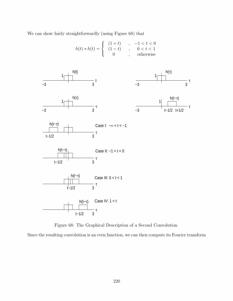
We can show fairly straightforwardly (using Figure 68) that

h(t) ∗ h(t) =

⎧⎪⎨⎪⎩

(1 + t) , −1 < t < 0(1− t) , 0 < t < 1

0 , otherwise

t−3 3

h(t)1

τ−3 3

h(τ)1

τ−3 3

h(τ)1

τ−3

1

t−1/2 t+1/2

h(t−τ)

τ3t−1/2

h(t−τ) Case I: −∞ < t < −1

τ3t−1/2

h(t−τ) Case II: −1 < t < 0

τ3t−1/2

h(t−τ) Case III: 0 < t < 1

τ3t−1/2

h(t−τ) Case IV: 1 < t

Figure 68: The Graphical Description of a Second Convolution

Since the resulting convolution is an even function, we can then compute its Fourier transform

220

directly as follows

F [h(t) ∗ h(t)] = 2∫ 1

0(1− t) cos(2πft)dt

=

[(1− t)2πf

sin(2πft)− 1

(2πf)2cos(2πft)

]∣∣∣∣∣1

0

=1− cos(2πf)

2(πf)2=

sin2(πf)

(πf)2

=sin(πf)

(πf)· sin(πf)

(πf)

This result, of course, is exactly what the convolution theorem predicts. (Note our use ofthe trigonometric identity

sin2(x) =1− cos(2x)

2. )

Therefore, on the one hand, we might say the convolution theorem, like any other transformrule, does not really provide any information that we could not obtain by direct computation.On the other hand, if all we had needed was F [h(t) ∗ h(t)] , using the convolution theoremwould have saved us significant computational effort. But, as we shall see in subsequentsections, the importance of the convolution theorem is not solely as a computational tool.The convolution theorem also provides fundamental insights into the behavior of physicalsystems, insights that would be extremely difficult to find without it.

We would close this section with one further thought. One of the powerful aspects ofFourier transform analysis is that, because of the similarity of the transform and its inverse,most time domain properties produce related frequency domain properties. This is also thecase with the convolution theorem, for we can fairly straightforwardly show that the Fouriertransform of the product of two functions produces a convolution of their transforms in thefrequency domain, i.e.

F [g(t) · h(t)] = G(f) ∗H(f) ≡∫ ∞

−∞G(φ)H(f − φ) dφ . (6.2.3)

We shall also see applications of this result in later sections.

221

PROBLEMS1. Compute, using the definition, the convolution ( h(t)∗ g(t) ) in the following cases. Then,in each case, compute the Fourier transform of the convolution and verify the result agreeswith the convolution theorem:

a. h(t) ={

2 , 0 < t < 20 , otherwise

g(t) ={e−t , 0 < t0 , otherwise

b. h(t) = g(t) ={

2 , −2 < t < 20 , otherwise

c. h(t) = e−|t| , −∞ < t <∞g(t) = cos(2πt) , −∞ < t <∞

222

6.3 Linear, Shift-Invariant Systems

One of the primary uses of the Fourier transform is in the analysis of what several authors(e.g. Gaskill) refer to as linear, shift-invariant systems. (So-called filters, which arise in signalprocessing, are one especially important instance of such systems.) Linear, shift-invariantsystems are, as we shall see, fundamental to much of engineering design. However, beforeproceeding any further, we first need to specify exactly what we mean by the term linear,shift-invariant system.

When we speak of a system, we mean any mathematical or physical process that can beessentially described by an input/output relationship. (Many control engineering texts usethe terms “plant” and system interchangeably.) In other words, a system is basically anyentity that can be described by the “black box” model

x(t) −→ S[ ] −→ y(t) ≡ S[x(t)]

input system output

Systems such as this arise any time we subject a physical object to some kind of force orcontrol mechanism, and are often described by differential equations where y(t) representsthe solution, and x(t) the applied force. Examples of systems defined by ordinary differentialequations are

y′′(t) + 3y′(t) + 2y(t) = x(t)

and

[y′(t)]2 + y(t) = x2(t) .(Note that the above diagram indicates that the input and output for a system both occur inthe same domain (in this case the “time” domain.) This contrasts with the Fourier transformbox we used earlier, where the inputs and outputs were in different (time and frequency,respectively) domains. Furthermore, the inputs and outputs (x(t) and y(t), respectively) toa system need not be limited to only scalars, but may be vectors as well.)

Systems may be either linear or nonlinear. A linear system, is one which obeys theprincipal of superposition, i.e. one in which the response (output) of that system to a sumof inputs is the sum of the responses (outputs) to the corresponding individual inputs. Interms of our black box model, a linear system must behave as follows

223

If x1(t) −→ S[ ] −→ y1(t)

and x2(t) −→ S[ ] −→ y2(t)

then ax1(t) + bx2(t) −→ S[ ] −→ ay1(t) + by2(t)

where x1(t) and x2(t) represent arbitrary inputs and a and b are arbitrary scalars.Lastly, a system is shift-invariant if delaying the input by an arbitrary amount produces

the identical response as to the undelayed input, except that the response is delayed by thesame amount as was the input, or, in terms of our black box model:

If x(t) −→ S[ ] −→ y(t)

then x(t− t0) −→ S[ ] −→ y(t− t0)

Shift-invariant behavior is so common that we perhaps take it for granted. But, anythingelse would make chaos of almost all engineering design! For example, how could we possiblybuild automobiles if turning the steering wheel clockwise produced right turns on Mondays,left turns on Tuesdays, no effect on Wednesdays, etc.?

With regards to the preceding discussion, you should realize that as far as systems areconcerned, linearity and shift invariance are independent considerations. For example, asystem may be linear, but not shift-invariant (e.g. the system represented by

y′′ + ty = x(t) )

or neither linear nor shift invariant (e.g. the system represented by

y′′ + tey = x(t) .)

In light of these comments, you should not be surprised to find that when linear, shift-invariant systems are expressed in terms of differential equations, the equations will belinear and constant coefficient.

Most engineering design focuses, at least initially, on linear, shift-invariant systems.Whether this is because most real-world systems can at least be approximated by them,

224

or whether it is just because these are the only ones for which explicit solutions are generallypossible is arguable, but the result is the same. Linear, shift-invariant systems are simplyfundamental to real applications.

For the purposes of our study, the mathematical importance of linear, shift-invariantsystems is that we can show, at least formally, that a system is linear and shift-invariant ifand only if its output is a convolution of the input with some other, system specific function,i.e., in terms of our black box model, a linear, shift-invariant system must obey the relation

x(t) −→ S[ ] −→ y(t) ≡ S[x(t)] =∫ ∞

−∞x(u)h(t− u)du

where h(t) is some function that depends solely on the particular system being considered,and not on x(t).

Formally showing that systems whose outputs are convolutions must be linear and shift-independent is extremely straightforward. Linearity follows immediately from basic calculusprinciples, since the integral of a sum is the sum of the integrals. Showing that the con-volution is also shift-invariant requires only a simple change of variables in the integral,i.e.

y(t− t0) =∫ ∞

−∞x(u)h((t− t0)− u)du

=∫ ∞

−∞x(u− t0)h(t− u)du ≡ S[x(t− t0)]

where we convert between the first and second integrals by replacing u in the first integralby (u− t0) everywhere.

Proving that a linear, shift-invariant systems must satisfy a convolution relationship is abit more involved. We start by considering some arbitrary interval, say from T0 to T1. Wenext divide this interval up into subintervals of equal length, denoting the endpoints of thesesubintervals as u0, u1, u2, . . . , uN , where u0 = T0 and uN = T1. We also let ∆u = ui+1 − ui.Then, because of its linearity, given any functions x(t) and w(t), the system must obey

N∑i=1

x(ui)w(t− ui)∆u −→ S[ ] −→N∑

i=1

x(ui)S[w(t− ui)]∆u

where S[w(t)] denotes the response (output) of the system to the input w(t). (The outputmust have this form because the ui are all constant values. Therefore the x(ui) are justnumbers, i.e. coefficients, and so the input is just a linear combination of the w(t − ui).Hence, since the system is linear, the output must be just the sum of the correspondingindividual responses.) However, both this input and output are in precisely the form of aRiemann sum approximation to a definite integral. Therefore, applying the same argumentsas we used in deriving the original Fourier transform identity in the previous chapter, weclaim that as ∆u→ 0, the system input/output relationship must become

225

∫ T1

T0

x(u)w(t− u)du −→ S[ ] −→∫ T1

T0

x(u)S[w(t− u)]du

But now, in the special case where T0 = −∞ and T1 = ∞ (a case which again reallyrequires some very delicate consideration of limiting processes), we can formally write that

∫ ∞

−∞x(u)w(t− u)du −→ S[ ] −→

∫ ∞

−∞x(u)S[w(t− u)]du

You should appreciate that we have derived this last relationship using no informationexcept that this system was linear, and assuming nothing about x(t) and w(t). We shallnow proceed, continuing to assume that x(t) is arbitrary, but limiting our attention to avery special w(t) - an impulse - i.e. w(t) = δ(t). In this case, the input/output black boxrelationship immediately above can be written

∫ ∞

−∞x(u)δ(t− u)du −→ S[ ] −→

∫ ∞

−∞x(u)S[δ(t− u)]du

or, using the sifting property of the delta function,

x(t) −→ S[ ] −→∫ ∞

−∞x(u)S[δ(t− u)]du

But we have also assumed that the system is shift-invariant. Therefore, if we denote theresponse of the system to the basic impulse δ(t) as h(t), i.e. if

h(t) = S[δ(t)]

or equivalently, if

δ(t) −→ S[ ] −→ h(t)

then, because of shift invariance, S[δ(t − u)] = h(t − u). Therefore, in summary, we haveshown that, for an arbitrary linear, shift invariant system,

x(t) −→ S[ ] −→∫ ∞

−∞x(u)h(t− u)du

Since δ(t) is an impulse, then h(t) as defined above is commonly referred to as the impulseresponse of the system. Therefore we may restate the conclusion of this discussion as beingthat the output of any linear, shift-invariant system is the convolution of the input with thesystem impulse response.

This last result expresses the fundamental behavior of linear, shift-invariant systems inthe time domain. But, as we have seen many times before, one of the central ideas of Fourier

226

analysis is that phenomena exist simultaneously in both the time and frequency domain.Therefore, for completeness, we should also interpret the input/output relationship of linear,shift-invariant systems in the frequency domain. But finding this interpretation is simple -the convolution theorem (6.2.2) tells us that, in the transform domain,

X(f) −→ S[ ] −→ X(f)H(f)

In this representation, of course, H(f) simply denotes the Fourier transform of the system’simpulse response, i.e.

H(f) =∫ ∞

−∞h(t)e−2πjftdt .

This transform is commonly also called the transfer function or frequency response of thesystem.

The fact that a linear, shift-invariant system’s output is a product in the frequencydomain turns out to be of immense value! Analyzing the responses of such systems to generalinputs in the time domain would require computing convolutions and, as you hopefullyappreciate from the examples we have already presented, both the mechanics of performingsuch computations and the subsequent visualization of the result can be fairly involved. Bycontrast, as a consequence of the convolution theorem, analyzing a system’s general behaviorin the frequency domain simply requires multiplying two curves together. This is usuallyvery straightforward and the result is generally quite easy to picture. For example, considerFigure 69. This figure clearly implies that the output of the system under consideration willbe a signal with all of the “low” frequencies from the original input unaffected, and all ofthe “high” frequencies lost. (Whether such an output is “good” or “bad” is a design issue,and not the point of the discussion here. The important point for us is that the frequencydomain/transfer function formulation of the system response lets us very quickly capture theessence of how this particular system affects input signals.)

The use of the frequency domain/transfer function formulation can also greatly simplifythe analysis and construction of complicated systems, by allowing a modular, building blockapproach. Specifically, suppose we have a system consisting of two serial subsystems, de-noted S1 and S2. Each of these subsystems will have its own impulse response and transferfunction, which we denote in the natural way, e.g. H2(f) would be the transfer function forsubsystem S2. In the frequency domain, the input/output diagram for this system becomes

X(f) −→ S1[ ] −→ H1(f)X(f) −→

−→ S2[ ] −→ H2(f)H1(f)X(f)

227

Figure 69: The Graphical Description of a System Output in the Transform Domain

But this diagram clearly implies that the resultant output would be the same as from asingle system whose transfer function were H1(f)H2(f). Even more importantly, it impliesthat we can replace any single, complicated system with a system made up of a number ofsimpler components, provided the product of the transfer functions of the components of thesimpler systems is identical to the transfer function of the more complicated system. Thisconclusion has far-reaching implications in terms of both design complexity and cost!

As the preceding discussion indicates, the impulse response and transfer function of asystem are pivotal to describing the behavior of that system and for designing systems tobehave in certain desired ways. (Of course, since the impulse response and transfer functionare a Fourier transform pair, knowledge of either uniquely determines the other and uniquelyand completely defines the system itself.) At this point though, the procedures for findingeither one are not clear. Therefore, we shall consider that question next.

6.4 Determining a System’s Impulse Response and Transfer Func-tion

Given the fundamental roles of the impulse response and transfer function in defining thebehavior of any given system, determining them becomes a crucial part of system design and

228

analysis. (Actually, as noted above, determining either one is, in concept, sufficient.) Wetherefore now consider the various ways in which either may be found, with special emphasison those techniques that apply not only to model (mathematical) systems, but also in the“real” world.

Theoretically, finding the impulse response for a system should be quite straightforward.After all, the impulse response is, by definition, just the system behavior resulting from animpulse force at t = 0. So why not just “hit” the system with an impulse and see whathappens? Mathematically, this is quite easily done - at least for systems which are modeledby constant coefficient ordinary differential equations. All we need to do is just replace theforcing function in the system’s differential equation by δ(t), zero out any initial conditionsand then solve, e.g. by Laplace transforms. For example, consider the RC circuit shownin Figure 70. At any time, the charge on the capacitor (Q(t)) and the applied externalvoltage (E(t)) are related by

Figure 70: A Sample RC Circuit

RdQ

dt+

1

CQ = E(t)

Therefore, if we take the “input” as the applied external voltage and the “output” as thevoltage measured across the capacitor, we can represent this system by the black box

E(t) −→ S[ ] −→ Vout(t) =1

CQ(t)

But the charge on the capacitor produced by a unit impulse voltage at t = 0 is simply thesolution to

RdQ

dt+

1

CQ = δ(t)

Q(0) = 0

Now, as noted earlier, constant coefficients and impulsive forcing terms generally dictatesolving by Laplace transforms. In this instance, taking the transform of both sides leads to

(Rs +

1

C

)L [Q(t)] = 1

229

or (using tables as appropriate)

L [Q(t)] =1

R

[1

s+ 1RC

]⇒ Q(t) =

⎧⎪⎪⎨⎪⎪⎩

1

Re−t/RC , t ≥ 0,

0 , otherwise

Converting the charge to the voltage on the capacitor shows that, by definition, the impulseresponse of this circuit is

h(t) =1

CQ(t) =

⎧⎪⎪⎨⎪⎪⎩

1

RCe−t/RC , t ≥ 0,

0 , otherwise

(6.4.4)

With the impulse response now available, we could now find this system’s transfer functionby Fourier transforming h(t). But note that this h(t) is clearly causal and has only finiteenergy. (You should view this as a fairly natural consequence of the fact that this was a“real” physical system.) Therefore, because we already have the Laplace transform of h(t),we can find its Fourier transform by one of the rules of the previous chapter, i.e. by simplyreplacing the variable s in the Laplace transform by the Fourier term (2πjf),

H(f) =1

CQ(f) =

1

C· 1

R· 1

2πjf + 1RC

=1

1 + 2πjfRC(6.4.5)

t

h(t)

+RC

+2RC

1

f

| H(f)|

1/RC+

−1/RC+

f

Θ(H(f))

1/RC−1/RC

pi/2

−pi/2

Figure 71: An Example Impulse Response and Transfer Function

(Both the impulse response and transfer function for this system are plotted in Figure 71.)Actually, since we know how to relate the Fourier transform of a derivative to the Fourier

transform of the original function, we could equally well have attacked this problem in thereverse order. That is, we could have first determined the transfer function by Fouriertransforming the differential equation. This would yield(

2πjfR +1

C

)Q(f) = 1⇒ Q(f) =

1

2πjfR + 1C

Because of the linearity of the transform, we could then divide by C to obtain the transformof the output (capacitor) voltage. This would, of course, yield the same H(f) as we found

230

above. Finally, inverse Fourier transforming this transfer function would produce the impulseresponse, h(t).

Mathematically, this approach - subjecting the system to an impulse - is direct, simple,and clearly applicable to any system described by a constant coefficient ordinary differentialequation. In general, the worst that we expect to encounter would be “nasty” algebra aspart of inverting the Laplace transform, or computing Fourier transform or inverse transformintegrals. However, subjecting a real system to an impulse may not be such a good idea!Real impulses are not that easy to generate - they can’t be truly instantaneous, but stillmust be of extremely short duration in order to adequately approximate a true impulse.Furthermore, because of their short duration, real impulses must also have very high am-plitudes. Unfortunately, high amplitudes, even when of short duration, can easily damagea real system - especially if sensitive electronics are involved. Therefore, some less stressfultesting method than impulse loading seems preferable for real systems. But what methodshould we then use?

One of the easiest forcing functions to generate, and one of the more harmless, is a simplesinusoid, e.g. AC current. (Of course, sinusoids are periodic, and there are no truly periodicfunctions. However, common sense argues that, provided we subject a system to a forcewhich is periodic over a sufficient length of time for all natural transients to die out, the(steady-state) response of the system should be essentially the same as the response to atruly periodic force.) But does the response of a system to a sinusoidal input shed any lighton the response of that same system to an impulse?

To find out, we select as our forcing function the complex exponential e2πjf0t, where f0

is some fixed frequency. In terms of our black box model and the properties of the impulseresponse, this produces the following input/output situation

e2πjf0t −→ S[ ] −→∫ ∞

−∞h(t− τ)e2πjf0τ dτ

But now, if we make the change of variables u = t− τ in the output integral (rememberingthat τ , not t is the variable of integration, we have∫ ∞

−∞h(t− τ)e2πjf0τ dτ =

∫ −∞

∞h(u)e2πjf0(t−u) (−du)

= e2πjf0t∫ ∞

−∞h(u)e−2πjf0u du

But this last integral is nothing more than, by definition, the Fourier transform of h(t)evaluated at the frequency f0! Thus, in terms of our black box model

e2πjf0t −→ S[ ] −→ e2πjf0tH(f0)

i.e. the output is simply the input sinusoid, multiplied by the value of transfer function atthat frequency. In other words, we can directly measure a system’s transfer function, just by

231

measuring the system’s response to a periodic (and almost certainly nondamaging) forcingfunction! (More precisely, |H(f0)| is the ratio of the amplitude of the output to the amplitudeof the input, and Θ (H(f0)) is the difference in phase between the output and input. Ofcourse, strictly speaking, such a measurement only tells us the transfer function at the singleforcing frequency f0. But we simply need to repeat the test, over any appropriate rangeof frequencies, in order to find the transfer function over that range. This testing methodhelps give the transfer function its other commonly-used name - the frequency response.)Moreover, once we have obtained the transfer function by this method, we can then findthe impulse response mathematically by just taking an inverse transform, thus completelyavoiding having to load the system with an impulse.

For systems described by constant coefficient ordinary differential equations, we can alsoimplement this last approach mathematically. We simply replace the forcing function in thedifferential equation with a complex exponential, then solve by undetermined coefficients forthe steady-state solution. For example, for the circuit shown in Figure 70, with an inputsignal of E(t) = e2πjf0t, the differential equation becomes

RdQ

dt+

1

CQ = e2πjf0t

By undetermined coefficients, the steady-state particular solution to this problem is

Q(t) =1

2πjf0R+ 1C

e2πjf0t =C

2πjf0RC + 1e2πjf0t

and therefore the response across the capacitor is

Vout(t) =1

CQ(t) =

1

2πjf0RC + 1e2πjf0t

Thus,

H(f0) =Vout(t)

e2πjf0t=

1

2πjf0RC + 1⇒ H(f) =

1

1 + 2πjfRC

This of course, is exactly the same transfer function as we found earlier, and we could nowagain determine the impulse response of this system (if we did not already know it) simplyby computing the inverse Fourier transform of this H(f).

There is one small practical problem with the above development. Complex-valued func-tions are really only mathematical artifices, and not producible in the “real” world. So whatdo we use as the actual input signal?

The answer is quite simple - we use cos(2πf0t)! As you should be able to verify from

232

basic trigonometric identities,

h(t) ∗ cos(2πf0t) =∫ ∞

−∞h(τ) cos(2πf0(t− τ)) dτ

= cos(2πf0t)∫ ∞

−∞h(τ) cos(2πf0τ) dτ

+ sin(2πf0t)∫ ∞

−∞h(τ) sin(2πf0τ) dτ

= cos(2πf0t) �e [H(f0)]− sin(2πf0t) �m [H(f0)]

Thus the real and imaginary parts of H(f0), respectively, can be found directly, with a realinput signal, just by measuring the amplitude of the output at two times - one in phase withthe input and the other 90o out of phase with the input.

We would close this section with one last point. The results presented here provide thebasic methods for computing the impulse response and transfer function of a given system.We would reemphasize that finding these is not just a mathematical exercise. The transferfunction is fundamental to analyzing the behavior of systems, since our earlier analysis oflinear, shift-invariant systems showed that the convolution theorem expresses the output ofsuch systems as a product of the transform of the input with the transfer function. Forexample, consider the transfer function we have calculated in this section (Figure 71). Fairlyclearly

|H(f)| ≈ 1 , f << 1/RC|H(f)| → 0 , f →∞

and so this system will pass “low” frequency components in the input relatively unaffected,but severely attenuate “high” frequencies. (Furthermore, because Θ (H(f)) /f is not con-stant, different frequency components in the input signal will be delayed by different amountsand become “out of step.”) In fact, if

X(f) = O

(1

f

)then X(f)H(f) = O

(1

f 2

)

In other words, this system will apparently sufficiently attenuate the high frequencies whichare necessary to produce discontinuities that, given a discontinuous input signal, the outputwill be continuous, with only a discontinuous derivative. Therefore, we expect this systemwill generally distort input signals. We may confirm this analysis by considering a sampleinput function, e.g. the one shown, together with the corresponding system output (Fig-ure 72). (This output was computed directly as the convolution of the input with (6.4.4).The computation is not presented here because, except for scaling terms, it is identical tothe first example in this chapter.) As expected, the output, while clearly related to theinput, is also not a “clean” copy, but a distorted one. (The similarities between this analysisand the one we conducted for the LRC circuit with periodic input in Chapter 2 are notcoincidental!)

233

Figure 72: An Example Input and Output for an RC Circuit

6.5 Applications of Convolution - Signal Processing and Filters

As indicated at the close of the last section, the importance of the Fourier transform, ofconvolution, of the transfer function, etc., is in their value as tools for analyzing physicalsystems. One of the most important application areas where they are used is in so-calledsignal processing. In signal processing, we start by assuming that some information-carryingsignal is initially transmitted into a physical medium. (For example, either an antenna maytransmit a radio signal into the atmosphere or a transducer may transmit a sonar signalinto water.) The medium is commonly referred to as the channel. After passing throughthe medium, the signal is received at some location. (This location is usually, but notalways, somewhere other than the transmitting location.) However, because of physicaleffects encountered while passing through the channel, or perhaps because of the presenceof more than one signal in the channel at the same time, the received signal is generallysome distorted or otherwise affected version of the original transmitted signal (in somewhatthe same way the output at the capacitor in our last example was a distorted version of theinput pulse). Schematically, we may represent this process as

x(t) −→ C [ ] −→ y(t)

Transmitted Signal Channel Received Signal

Signal processing then tries to design some circuit, etc., which, if we pass the receivedsignal (y(t)) through it, will “undo” the effects introduced by the channel, resulting in anoutput that is reasonably close to the original transmitted signal, i.e.

y(t) −→ S[ ] −→ p(t) (≈ x(t))

Received Signal Processing Output

(Of course, ideally we would like to have p(t) equal x(t).)The simplest model of such a situation occurs when the channel is linear and shift-

invariant. Then the channel has its own transfer function, which we denote Hc(f), andtherefore the transform of the received signal would be

234

Y (f) = Hc(f)X(f)

But theoretically, if this is true, all we need to do is design the processing system so that itstransfer function is the reciprocal of that of the channel, i.e.

Hs(f) =1

Hc(f)⇒ P (f) = Hs(f)Y (f) =

1

Hc(f)·Hc(f)X(f) ≡ X(f)

Unfortunately, for several reasons, only some of which we will touch on here, we usually can’treach this ideal in real problems. For one reason, in many cases we can’t even completelyspecify all the effects of the channel - which makes it very difficult to remove them! However,we may nevertheless often reverse the primary corrupting effects of the channel, and recoveran effectively fully usable version of the transmitted signal.

Perhaps the most basic type of signal processing involves filters. As their name implies,filters let some “things” through and reject others. The simplest filters are designed to letcertain frequencies through and block (or attenuate) the remaining ones. Such filters fallinto three general categories, which are almost self-defining

• Low-pass Filters - which allow low frequencies through but block high ones;

• High-pass Filters - which allow high frequencies through and block low ones; and

• Band-pass Filters - which block both very low and very high frequencies, but passthose in some intermediate range

Figure 73: Transfer Functions for Ideal Filters

235

Figure 73 displays the transfer functions for the ideal cases of each of these. We call theseideal cases because, none of them are in fact physically achievable. The reason they arenot is essentially the same in each case - they represent systems that are not causal. Forexample, the transfer function for the ideal low-pass filter is

HLP (f) ={

1 , |f | < f0

0 , otherwise

Unfortunately, this means that the impulse response for this filter is

hLP (t) =sin(2πf0t)

πt

and, as already indicated, this is not a causal system. On the other hand, causal systemswith reasonably the same performance are realizable. For example, the RC system describedin Figure 70 is easily to build, quite inexpensive, and, according to Figure 71, reasonably ableto pass low frequencies but block high ones, provided we select R and C appropriately. High-pass and band-pass filters can be similarly realized by simply combining appropriately-valuedresistors, capacitors and inductors, and measuring the output voltage on the appropriatedevice. The (magnitudes of the) transfer functions for all of these circuits are shown inFigure 74. Similar filters are common in virtually all home electronics. For example, a band-pass filter, consisting of an LRC circuit with a variable capacitor, is found in the tuningcontrol of virtually every radio. Varying the capacitor adjusts the frequency at center of thepass-band and effectively selects, from all the frequencies received, signals with only thatfrequency.

E(t)

VC

CR

h(t)

t

1|H(f)|

f

1

E(t)

VR

CR

h(t)

t

|H(f)|

f

1

E(t)

VR

CR L

h(t)

t

|H(f)|

f

1

LC1/(2π√⎯⎯ )LC−1/(2π√⎯⎯ )

Figure 74: Real Filters With Their Impulse Responses and Transfer Functions. Top showRC filter (lo-pass),middle is RC filter (high-pass), and bottom is LRC filter (band-pass)

At this juncture, we shall close our discussion of filters and, to a reasonable degree, oflinear, shift-invariant systems as well. We hope we have at least reasonably well set out theirimportance in engineering systems design, and the pivotal role the transfer function plays intheir use. We are not however done with the Fourier transform yet, but will examine insteadsome of its other applications.

236

6.6 Applications of Convolution - Amplitude Modulation and Fre-quency Division Multiplexing

As we have previously alluded to, one attractive feature of the Fourier transform is the man-ner in which the near-symmetry between the transform and inverse transform operationsimplies that almost every time-domain property has a near mirror-image in the frequencydomain. One instance of this is our earlier-mentioned converse to the convolution theo-rem (3), which we repeat here

F [g(t) · h(t)] = G(f) ∗H(f)

We now investigate one of the most common applications of this result.Commercial radio broadcasts originally utilized what we call amplitude modulation. (The

first commercial radio stations were also limited to using only a fairly narrow band of broad-cast frequencies in the low MHz range. Because of the modulation used by virtually all ofthese early stations, this band of frequencies is generally still referred to as the AM band.)In amplitude modulation, the actual information signal, e.g. a talk show or music, consti-tutes what is generally referred to as the baseband signal, which we denote here as m(t).We commonly refer to the range of frequencies which comprise the baseband, i.e. which arepresent in its Fourier transform (M(f)), as its bandwidth, which we denote by B. (In AMradio, the baseband bandwidth is generally limited to a relatively narrow range of low (lessthan 5 KHz) frequencies.) Amplitude modulation consists of electronically multiplying thisbaseband signal by a high frequency sinusoid - the so called carrier signal, which we shallrepresent as cos(2πf0t) - to produce the broadcast signal, which we denote s(t) (Figure 75).(The carrier frequency (f0) is typically in the MHz range.) In the time domain then, the re-sulting broadcast signal may be viewed as a very rapid oscillation within the envelope definedby the slowly varying baseband signal. The term amplitude modulation aptly describes thisprocess because, as the figure shows, the amplitude of the carrier is modified (modulated)according to the amplitude of the baseband signal.

Figure 75: Amplitude Modulation - The Time Domain View

237

The frequency domain interpretation of amplitude modulation turns out to be quiteintriguing. Specifically, according to (6.2.3), in the transform domain

S(f) = F [s(t)] = F [m(t) · cos(2πf0t)] = M(f) ∗ F [cos(2πf0t)]

= M(f) ∗[1

2δ(f − f0) +

1

2δ(f + f0)

]

=∫ ∞

−∞M(f − φ)

[1

2δ(φ− f0) +

1

2δ(φ+ f0)

]dφ

=1

2

∫ ∞

−∞M(f − φ)δ(φ− f0) dφ+

1

2

∫ ∞

−∞M(f − φ)δ(φ+ f0) dφ

But the sifting property of the delta function simplifies the two last integrals here, and showsthat the transform of the broadcast signal is simply

S(f) =1

2M(f − f0) +

1

2M(f + f0) (6.6.6)

Figure 76: Amplitude Modulation - The Frequency Domain View

The graphical interpretation of this result in the frequency domain is both straightforwardand elegant. Specifically, (6.6.6) say that S(f) consists of precisely two half-size copies of thetransform of the original baseband signal. One copy is centered about f0, the other about−f0

(Figure 76). (For graphical convenience, we have chosen to represent M(f) in this figure asa real, even function. While the following discussion uses that fact, our conclusions remainvalid, with at most minor modifications, in the case of a complex M(f).)

Figure 76 also helps to explain another commonly occurring variant of amplitude modula-tion. In this figure, because of the even symmetry of M(f), the part of the spectrum of S(f)between (f0 − B) and f0 is clearly totally redundant of that part between f0 and (f0 + B).(These two parts are referred to, respectively, as the lower and upper sidebands of the trans-mitted signal.) But if the lower sideband contains no information not also available in theupper sideband, why bother to transmit both? The answer is we don’t need to. We could

238

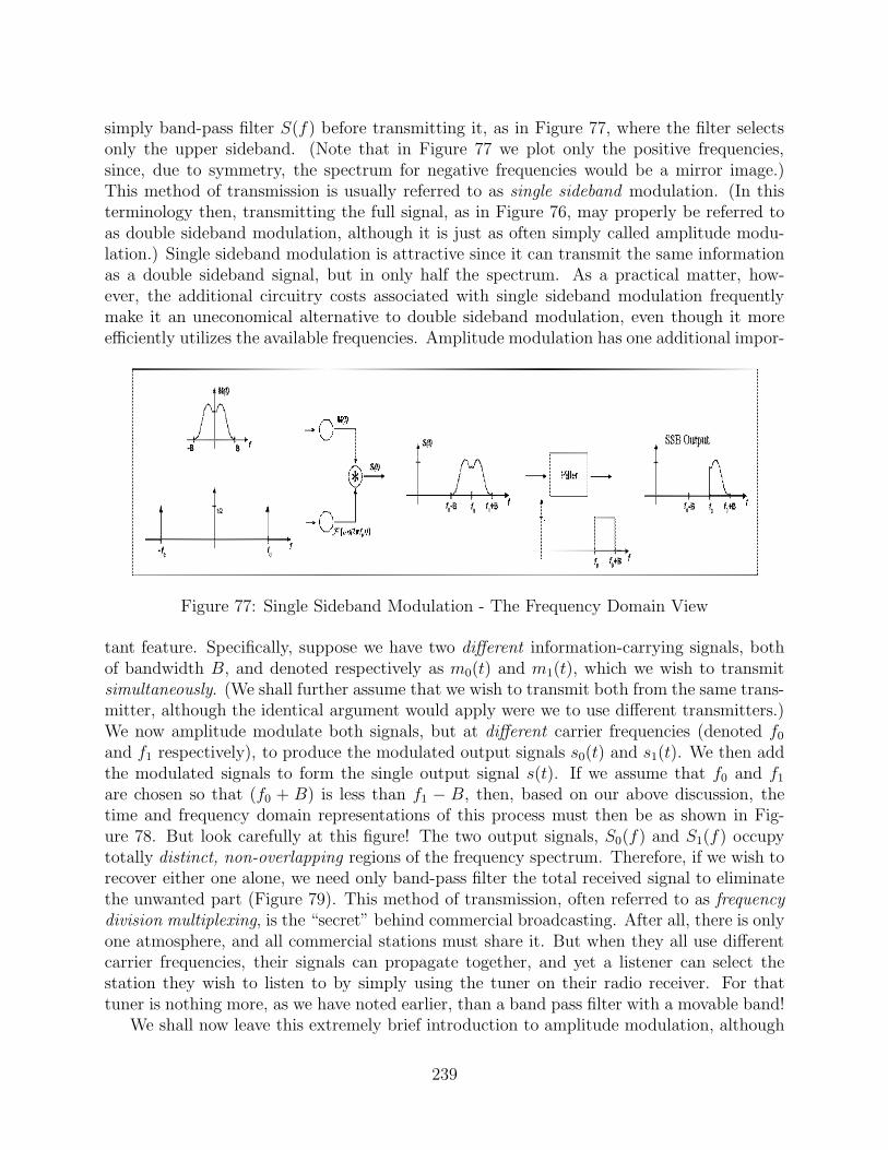
simply band-pass filter S(f) before transmitting it, as in Figure 77, where the filter selectsonly the upper sideband. (Note that in Figure 77 we plot only the positive frequencies,since, due to symmetry, the spectrum for negative frequencies would be a mirror image.)This method of transmission is usually referred to as single sideband modulation. (In thisterminology then, transmitting the full signal, as in Figure 76, may properly be referred toas double sideband modulation, although it is just as often simply called amplitude modu-lation.) Single sideband modulation is attractive since it can transmit the same informationas a double sideband signal, but in only half the spectrum. As a practical matter, how-ever, the additional circuitry costs associated with single sideband modulation frequentlymake it an uneconomical alternative to double sideband modulation, even though it moreefficiently utilizes the available frequencies. Amplitude modulation has one additional impor-

Figure 77: Single Sideband Modulation - The Frequency Domain View

tant feature. Specifically, suppose we have two different information-carrying signals, bothof bandwidth B, and denoted respectively as m0(t) and m1(t), which we wish to transmitsimultaneously. (We shall further assume that we wish to transmit both from the same trans-mitter, although the identical argument would apply were we to use different transmitters.)We now amplitude modulate both signals, but at different carrier frequencies (denoted f0

and f1 respectively), to produce the modulated output signals s0(t) and s1(t). We then addthe modulated signals to form the single output signal s(t). If we assume that f0 and f1

are chosen so that (f0 + B) is less than f1 − B, then, based on our above discussion, thetime and frequency domain representations of this process must then be as shown in Fig-ure 78. But look carefully at this figure! The two output signals, S0(f) and S1(f) occupytotally distinct, non-overlapping regions of the frequency spectrum. Therefore, if we wish torecover either one alone, we need only band-pass filter the total received signal to eliminatethe unwanted part (Figure 79). This method of transmission, often referred to as frequencydivision multiplexing, is the “secret” behind commercial broadcasting. After all, there is onlyone atmosphere, and all commercial stations must share it. But when they all use differentcarrier frequencies, their signals can propagate together, and yet a listener can select thestation they wish to listen to by simply using the tuner on their radio receiver. For thattuner is nothing more, as we have noted earlier, than a band pass filter with a movable band!

We shall now leave this extremely brief introduction to amplitude modulation, although

239

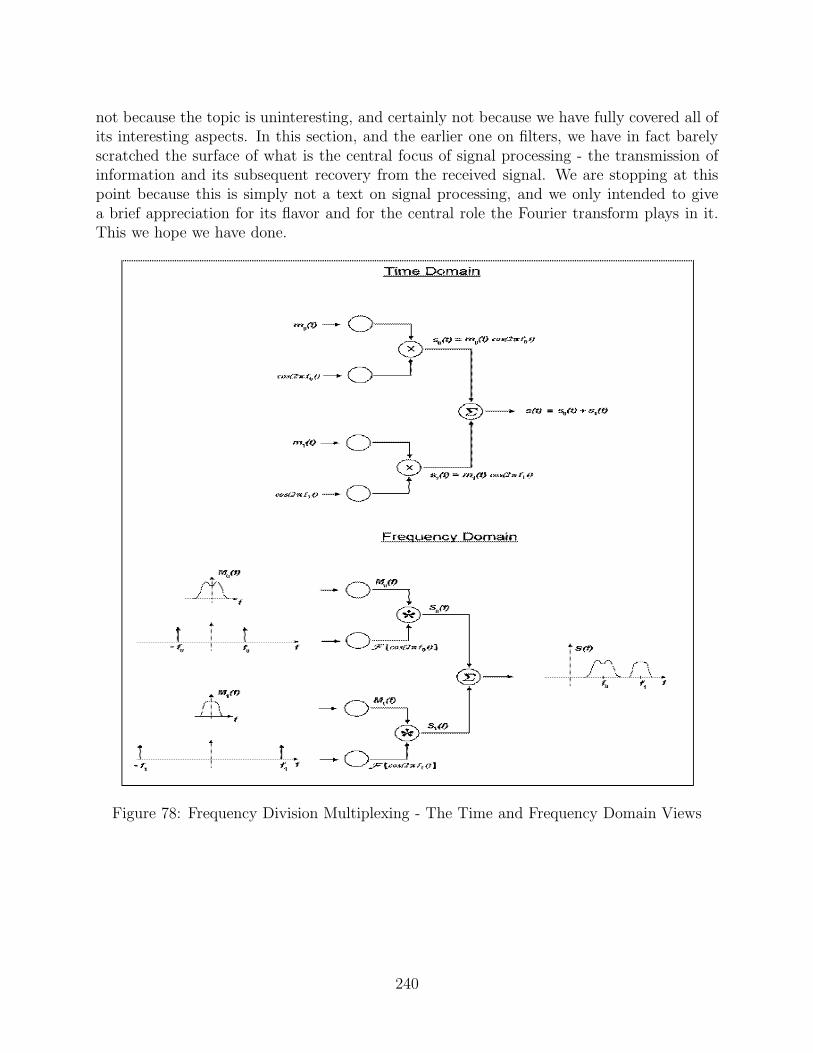
not because the topic is uninteresting, and certainly not because we have fully covered all ofits interesting aspects. In this section, and the earlier one on filters, we have in fact barelyscratched the surface of what is the central focus of signal processing - the transmission ofinformation and its subsequent recovery from the received signal. We are stopping at thispoint because this is simply not a text on signal processing, and we only intended to givea brief appreciation for its flavor and for the central role the Fourier transform plays in it.This we hope we have done.

Figure 78: Frequency Division Multiplexing - The Time and Frequency Domain Views

240

Figure 79: Recovering a Frequency Division Multiplexed Signal

241

6.7 The D’Alembert Solution Revisited

We now turn to the application of the Fourier transform in a totally different context thansignal processing - the study of wave propagation. (Actually, we can also apply several ofthe ideas which we shall discuss here to image processing, which can be loosely thought ofas the signal processing of photographic or other images in order to improve their quality.)The biggest single difference between this application and our earlier discussion on signalprocessing is that we are now going to be computing transforms with respect to a differentvariable - a spatial one (x) rather than time (t).

Mathematically, changing the symbol of the variable we consider makes effectively nodifference. For example, if we have a function, denoted f(x), we could equally well define aspatial Fourier transform by rewriting the fundamental Fourier transform relationships ((13)and (14) in Chapter 5) as

F (k) = F [f(x)] =∫ ∞

−∞f(x)e−2πjkxdx (6.7.7)

f(x) = F−1[F (k)

]=∫ ∞

−∞F (k)e2πjkxdk (6.7.8)

Formally, all this requires is using the symbol k instead of f , and x instead of t. (We alsochoose to write the overhead tilde here just to continually remind ourselves that this is aspatial, rather than a temporal Fourier transform. Other than serving as this reminder, thetilde is extraneous.) Moreover, with the proper change of symbols, all of the rules of Fouriertransforms are still valid, e.g.

F[df

dx

]= (2πjk)F (k) ,

etc. Physically, of course, using the spatial Fourier transform will require that several inter-pretations change. For example, the discussion will now often be in terms of wavelengths,rather than frequencies.

One additional important factor comes into play when the spatial Fourier transform isapplied to the study of wave phenomena. This addition is necessary because, as we sawin the earlier chapters of this text, most wave phenomena involve functions of two or moreindependent variables, and are described by partial differential equations. Therefore we dohave to consider, briefly, how to interpret the transform of a function of two variables withrespect to only one of them, i.e. how to interpret

F [u(x, t)]

This is actually not difficult, provided we carefully keep track of the variables involved, andremember that the spatial Fourier transform is with respect to x, not t. Specifically, bydefinition, we may then write

F [u(x, t)] ≡ Uk(t) =∫ ∞

−∞u(x, t)e−2πjkx dx

242

Note that we have also slightly modified our notation here by writing the transform variable kas a subscript. We do this to emphasize that, in problems of this type, k is generally treatedas a parameter rather than as an independent variable. (In other words, transforming theproblem corresponds in effect to looking at how the solution evolves with respect to time ona frequency-by-frequency basis.) The result of the spatial transform of partial derivativescan be determined in the same manner we investigated the time transform of ordinary timederivatives, i.e. by starting with the definition and integrating by parts. The only differenceis that we now must carefully distinguish between the transforms of partials with respect tothe variable we are transforming on and those of partials of other variables, i.e. the transformof a partial with respect to x (the transform variable) behaves like

F[∂u

∂x(x, t)

]=∫ ∞

−∞∂u

∂x(x, t)e−2πjkx dx

= u(x, t)e−2πjkx∣∣∣∞x=−∞ −

∫ ∞

−∞u(x, t)

∂

∂x

[e−2πjkx

]dx

= −∫ ∞

−∞u(x, t)(−2πjk)

[e−2πjkx

]dx

= (2πjk)∫ ∞

−∞u(x, t)e−2πjkx dx

≡ (2πjk)Uk(t)

(6.7.9)

but the transform of a partial with respect to t (which is not the transform variable) becomes

F[∂u

∂t(x, t)

]=∫ ∞

−∞∂u

∂t(x, t)e−2πjkx dx

=d

dt

[∫ ∞

−∞u(x, t)e−2πjkx dx

]

≡ d

dtUk(t) =

dUk

dt

(6.7.10)

Of course, as with the Fourier time transform, these results can be extended to higherderivatives, e.g.

F[∂2u

∂x2(x, t)

]= (2πjk)2Uk(t) (6.7.11)

and

F[∂2u

∂t2(x, t)

]=d2Uk

dt2(6.7.12)

With these preliminaries out of the way, we now consider the one-dimensional waveequation in a region without boundaries, with an initial displacement but no initial velocity,

243

i.e. the problem∂2u

∂t2= c2

∂2u

∂x2, −∞ < x <∞ , 0 < t

u(x, 0) = f(x)∂u

∂t(x, 0) = 0

Of course, we have already seen that this problem can be solved by D’Alembert’s principle.However, it is nevertheless instructive to also apply the spatial Fourier transform here. (Notethat in terms of the time variable, this problem has the character of an initial value problem.Therefore, taking a Fourier transform with respect to time would not be sensible anyway,since initial conditions in the transform variable have no real meaning in the context ofFourier transforms. The only transform with respect to time that we could apply here wouldbe a Laplace transform - but that’s a different issue!) If we simply spatially Fourier transformboth sides of the partial differential equation

F[∂2u

∂t2(x, t)

]= F

[c2∂2u

∂x2(x, t)

](6.7.13)

and use (6.7.11) and (6.7.12) , we have

d2Uk

dt2= −(2πck)2Uk , (6.7.14)

which is just an ordinary differential equation for Uk(t). Since it is second-order however, westill need two initial conditions (in the transform domain) in order to find a unique solution.But where do these come from? The answer should be obvious. We had two initial conditionsin the original (spatial) domain! So why not transform them? If we do, we obtain

F [u(x, 0)] ≡ Uk(0) =∫ ∞

−∞f(x)e−2πjkx dx ≡ Fk

and

F[∂u

∂t(x, 0)

]≡ dUk

dt(0) = 0 ,

respectively. Combining all of these results in the single problem statement

d2Uk

dt2= −(2πck)2Uk

Uk(0) = Fk

dUk

dt(0) = 0

The solution to this is easily seen to be

Uk(t) = Fk cos(2πckt)

244

But, of course, this is the solution in the transform domain. To find the solution in theoriginal physical (spatial) domain, we must invert

u(x, t) ≡ F−1[Uk(t)

]=∫ ∞

−∞Uk(t)e

2πjkx dk

=∫ ∞

−∞Fk cos(2πckt)e2πjkxdk

But if we now apply Euler’s formula to the cosine term, we have

u(x, t) =∫ ∞

−∞Fk

[1

2

(e2πjckt + e−2πjkct

)]e2πjkx dk

=1

2

∫ ∞

−∞Fke

2πjckte2πjkx dk +1

2

∫ ∞

−∞Fke

−2πjkcte2πjkx dk

=1

2

∫ ∞

−∞Fke

2πjk(x+ct) dk +1

2

∫ ∞

−∞Fke

2πjk(x−ct) dk

(6.7.15)

However, according to our formulation for the inverse transform (6.7.8),

f(x) =∫ ∞

−∞Fke

2πjkx dk

Comparing this last equation to the two integrals in the previous one, we see that all threeare identical, except that the two integrals comprising u(x, t) are evaluated not at x, butat (x+ ct) and (x− ct) respectively, i.e.

u(x, t) =1

2f(x+ ct) +

1

2f(x− ct)

This, of course, is just D’Alembert’s principle. What should be interesting about the abovedevelopment is the manner in which the spatial Fourier transform permits us to derive theprinciple and so better understand how it arises. Knowing how a formula arises is generallyfar preferable to simply stating the formula - as if it arose by magic. But, as we shall seein the next section, the utility of the spatial Fourier transform is not just limited to thisderivation.

6.8 Dispersive Waves

In addition to providing a derivation of D’Alembert’s principle, the spatial Fourier transformalso allows us to study other wave propagation problems to which D’Alembert’s principlesimply does not even apply. For example, consider the problem

∂2u

∂t2= c2

∂2u

∂x2− u

u(x, 0) = f(x)∂u

∂t(x, 0) = 0

(6.8.16)

245

We shall not dwell on the physics that introduce the additional (−u) term here. Howeverthere are real physical models, such as transmission lines, for which this equation is a model.Our intent is solely to demonstrate the information the spatial Fourier transform can provideabout the solutions to this problem, and how these solutions may differ from those of the“pure” one-dimensional wave equation.

It is fairly easily shown that neither of the functions F (x − ct) nor G(x + ct) satisfythe partial differential equation in (6.8.16). Therefore, for this problem, a D’Alembert-type solution is not feasible. However, because this partial differential equation is linearand constant coefficient, transform methods still are. Therefore we shall simply proceed todirectly transform the partial differential equations and boundary conditions. If we do this ina similar manner to our derivation of (6.7.13)-(6.7.13), and the associated initial conditions,we find

d2Uk

dt2= −

[1 + (2πck)2

]Uk

Uk(0) = Fk

dUk

dt(0) = 0

The solution to this may be written in the following form

Uk(t) = Fk cos(2πckνkt) , (6.8.17)

where we define

νk =

√1 +

1

(2πck)2(6.8.18)

(The reason introducing νk is most likely not transparent at this point. However, as we shallsee, it simplifies the following analysis somewhat.) Again, as in the previous problem, werecognize that (6.8.17) represents the solution in the transform domain, and so must beinverted. With the exception of the addition of the νk term, this process is identical to theprevious inversion, and can be shown to lead to

u(x, t) =1

2

∫ ∞

−∞Fke

2πjk(x+νkct) dk +1

2

∫ ∞

−∞Fke

2πjk(x−νkct) dk

Here however, we cannot simplify the result as we did in the D’Alembert problem. Thedifficulty is the νk term, which makes neither integral a function of a simple expressionlike (x − ct). (Of course, since k is the variable of integration, we cannot take νk outsidethe integral!) However, we can still obtain some insights. Specifically, consider the secondintegral

1

2

∫ ∞

−∞Fke

2πjk(x−νkct) dk

Since this integral arose from an inverse transform, we must view it as the analog of theFourier series, i.e. as the attempt to reconstruct the physical function by combining its

246

components over all (spatial) frequencies (or equivalently over all wavelengths). Any one ofthese particular components is described by

1

2Fke

2πjk(x−νkct)

for a fixed value of k. This expression clearly represents a wave, of a single wavelength,

and amplitude1

2Fk, moving to right, but with velocity cνk, not c. (A similar analysis and

conclusion can be made on the other integral, except of course the wave there moves to theleft.) But νk depends on k. In other words, the frequency components that made up theinitial displacement (f(x)) propagate at different speeds. Therefore, as time evolves, theywill become progressively more “out of step,” or disperse. (For this reason, this problemis commonly called the dispersive wave equation.) Thus, while we apparently still havepropagation in this case, as time passes the dispersion will cause an increasing distortion ofthe shape of the propagating disturbance relative to the original displacement. By contrast,in the D’Alembert inverse (6.7.15), all components move at velocity c, and therefore remain“in step,” causing the original displacement not to lose shape as it propagates. Figure 80displays the graphs of the solution to a dispersive wave equation, computed by numericallyevaluating the integrals involved. The important point of this figure is that the computedintegrals substantiate our intuitive expectation, an expectation which came directly fromFourier transform analysis.

Figure 80: Solutions of a Dispersive Wave Equation at Different Times

With this section, we close our brief introduction to the spatial Fourier transform. Aswith our discussion of signal processing, this discussion was not intended to be either in-depth or all-inclusive. On the contrary, our only intention was to provide a brief flavor of

247

another instance where Fourier methods provide powerful insights into the workings of thephysical world. As with our earlier introduction to signal processing, we hope these shortsections have accomplished this for the spatial Fourier transform.

6.9 Correlation

There is one further time-domain operation that is commonly associated with the Fouriertransform. This is the so-called correlation, which is defined as

x(t) � y(t) ≡∫ ∞

−∞x(τ)y(t+ τ) dτ (6.9.19)

In form, correlation looks quite close to convolution, except correlation uses the term (t+ τ)in the integrand, vice (t−τ) in convolution. On the other hand, the uses and interpretationsof correlation and convolution are widely different. Correlation is most often used to measurethe similarity between signals, especially when one has been contaminated by noise. Becauseof the forms of convolution and correlation look quite close, the Fourier transform of acorrelation produces a very similar, though not identical, result to the convolution theorem.For the sake of completeness, we shall present that result here. We start, as usual, with theformal definition

F [x(t) � y(t)] ≡∫ ∞

−∞

{∫ ∞

−∞x(τ)y(t+ τ) dτ

}e−2πjft dt

As with the convolution theorem, because this is a two-dimensional integral, we may at leastformally interchange the order of integration, yielding

=∫ ∞

−∞

{∫ ∞

−∞x(τ)y(t+ τ)e−2πjft dt

}dτ

But then, because the inner integral does not depend on τ , we may move x(τ) outside of theinner integral, yielding

=∫ ∞

−∞x(τ)

{∫ ∞

−∞y(t+ τ)e−2πjft dt

}dτ

and since the inner integral now corresponds to the Fourier transform of y(t), shifted by (−τ),we may use the shift rule to write

=∫ ∞

−∞x(τ)Y (f)e−2πjf(−τ) dτ

But since Y (f) does not depend on the variable of integration, we may now take it completelyoutside the integral, and write

= Y (f)∫ ∞

−∞x(τ)e−2πj(−f)τ dτ

However, by definition, the remaining integral is simply the Fourier transform of x(t), butevaluated at (−f), i.e.

248

F [x(t) � y(t)] = Y (f)X(−f) (6.9.20)

(It’s fairly important to note here that, unlike the convolution, correlation is generally notcommutative, i.e. in general

x(t) � y(t) = y(t) � x(t)

This is reflected in (6.9.20) because, in general

Y (f)X(−f) = X(f)Y (−f)

Dealing with transforms of correlations is thus quite a bit more delicate than dealing withthe transforms of convolutions. Regrettably, we shall not pursue this any further at thispoint.)

Beyond presenting this result (6.9.20), we shall not delve further into the uses of correla-tion. Nevertheless, it does represent one more operation which, in the proper context, maybe better understood in the frequency domain, via the Fourier transform, than in the timedomain.

6.10 Summary

In this chapter, we have briefly covered some of the classic applications of the Fourier Trans-form - signal processing, modulation, and wave propagation. As we noted several times,our coverage of each was very abbreviated, and only designed to show how the transformproduces insights that might be very difficult to arrive at by any other means. The keypoint here is the ability with the transform, as with the Fourier series, to provide two viewsof a physical phenomenon - one in the time domain, the other in the frequency domain.Depending on which aspect of a particular phenomenon is of primary interest will usuallydetermine which domain is the most appropriate to study the problem in.

249

PROBLEMS

1. Consider the linear, shift-invariant system represented by the following circuit

LdI

dt+RI = E(t)

Vout = RI

a. Directly determine, e.g. using the Laplace transform, the impulse response of thissystem. Sketch this response.

b. (1) Find the Transfer function of this system by computing the Fourier transform ofthe impulse response determined in part a. above.

b. (2) Show that the alternative method of finding the Transfer function, i.e. as theresponse of a system to the forcing function e2πjf0t , produces the same result as in part (1),

c. Sketch the amplitude and phase spectra of the Transfer function computed in part b.

2. Repeat problem 1 for the same circuit, except with the output taken as the voltage acrossthe inductor, i.e.

LdI

dt+RI = E(t)

Vout = LdIdt

250

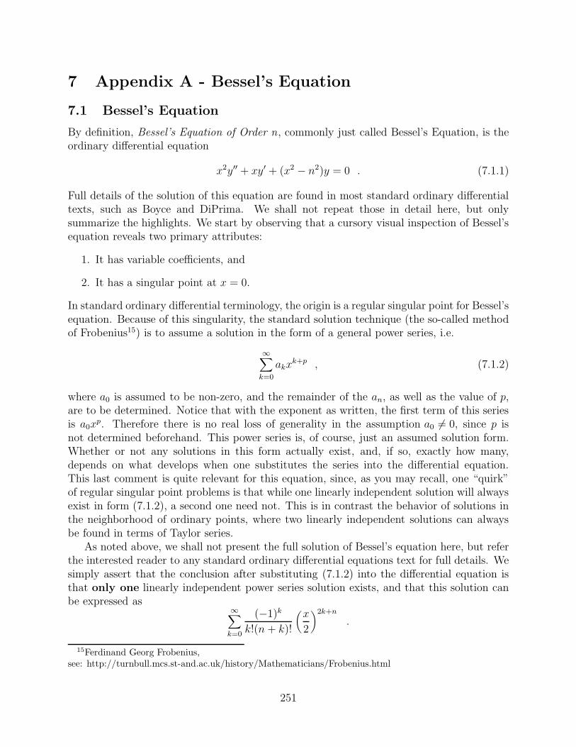
7 Appendix A - Bessel’s Equation

7.1 Bessel’s Equation

By definition, Bessel’s Equation of Order n, commonly just called Bessel’s Equation, is theordinary differential equation

x2y′′ + xy′ + (x2 − n2)y = 0 . (7.1.1)

Full details of the solution of this equation are found in most standard ordinary differentialtexts, such as Boyce and DiPrima. We shall not repeat those in detail here, but onlysummarize the highlights. We start by observing that a cursory visual inspection of Bessel’sequation reveals two primary attributes:

1. It has variable coefficients, and

2. It has a singular point at x = 0.

In standard ordinary differential terminology, the origin is a regular singular point for Bessel’sequation. Because of this singularity, the standard solution technique (the so-called methodof Frobenius15) is to assume a solution in the form of a general power series, i.e.

∞∑k=0

akxk+p , (7.1.2)

where a0 is assumed to be non-zero, and the remainder of the an, as well as the value of p,are to be determined. Notice that with the exponent as written, the first term of this seriesis a0x

p. Therefore there is no real loss of generality in the assumption a0 = 0, since p isnot determined beforehand. This power series is, of course, just an assumed solution form.Whether or not any solutions in this form actually exist, and, if so, exactly how many,depends on what develops when one substitutes the series into the differential equation.This last comment is quite relevant for this equation, since, as you may recall, one “quirk”of regular singular point problems is that while one linearly independent solution will alwaysexist in form (7.1.2), a second one need not. This is in contrast the behavior of solutions inthe neighborhood of ordinary points, where two linearly independent solutions can alwaysbe found in terms of Taylor series.

As noted above, we shall not present the full solution of Bessel’s equation here, but referthe interested reader to any standard ordinary differential equations text for full details. Wesimply assert that the conclusion after substituting (7.1.2) into the differential equation isthat only one linearly independent power series solution exists, and that this solution canbe expressed as

∞∑k=0

(−1)k

k!(n + k)!

(x

2

)2k+n

.

15Ferdinand Georg Frobenius,see: http://turnbull.mcs.st-and.ac.uk/history/Mathematicians/Frobenius.html

251

The function represented by this series is conventionally referred to as the Ordinary BesselFunction of the First Kind of Order n, or more commonly as simply the Bessel Function ofOrder n. It is virtually universally represented by the symbol Jn(x), i.e.

Jn(x) ≡∞∑

k=0

(−1)k

k!(n+ k)!

(x

2

)2k+n

. (7.1.3)

Of course, like any second order linear equation, Bessel’s equation requires two linearlyindependent solutions in order to construct the general solution. However, according thediscussion just completed, any solution which is independent of Jn(x) cannot be written asa “pure” power series, and therefore must be determined by some procedure other than themethod of Froebenius. Fortunately, there are several such techniques available for determin-ing a second, linearly independent solution, to an ordinary differential equation, once a firstone is known. One general method is reduction of order. A second option, more tailoredto this specific type of problem, involves careful differentiation of the series solution withrespect to the parameter p. Either of these methods could be applied here to generate asolution which is linearly independent of Jn(x).

As before, we omit any details of this actual construction of this second linearly inde-pendent solution to Bessel’s equation. (Again, these can be found in standard texts. Beforecontinuing, however, one slight word of caution, is in order. You should recall that there is nosuch thing as a unique set of linearly independent solutions to any second-order differentialequations. For example, we could represent the solution to

y′′ − y = 0

equally well as eithery(x) = c1e

x + c2e−x

ory(x) = d1e

x + d2 cosh(x) .

Therefore, occasionally, other texts or papers may use different formulas or symbols thanthe ones we shall present. However our choice and notation are extremely common.)

Probably the most frequently used choice for the second solution to Bessel’s equation isthe function almost universally denoted by Yn(x), which has the rather imposing definition

Yn(x) = −1

π

n−1∑k=0

(n− k − 1)!

k!

(x

2

)2k−n

+2

πln(x

2

)Jn(x)

−1

π

∞∑k=0

{ψ(k + 1) + ψ(n + k + 1)} (−1)n

k!(n+ k)!

(x

2

)2k+n

(7.1.4)

whereψ(1) = −γ

ψ(k) = −γ +k−1∑i=1

1

i

252

and γ is a constant, commonly called Euler’s16 constant. Like π, the value of Euler’s constantcannot be determined exactly, but is approximately γ = 0.57721566 . . .. With the caveatthen that our notation is almost, but not quite, universal, we finally arrive at the conclusionthat the general solution to (7.1.1) may be represented

y(x) = c1Jn(x) + c2Yn(x) .

7.2 Properties of Bessel Functions

Bessel functions occur in a wide variety of applications. Because of their frequent appearance,they have been studied in great detail for well over a hundred years. These studies haveuncovered many quite interesting properties and relationships, some of the more importantof which we shall now briefly consider. (More comprehensive listings of these may be foundin standard reference texts such as Abramowitz and Stegun, or Spanier and Oldham.)

At least initially, both the qualitative and quantitative properties of Bessel functions areobscured by the infinite series involved in their definitions ((7.1.3) and (7.1.4)). However,in one sense, these series are not as “bad” as they might be. Both series can be shownto converge at all values of x (by the ratio test), and both are alternating term series, i.e.they change sign every term. Furthermore, for “large” k, the denominators grow approxi-mately as (k!)2. Therefore, for most “reasonable” values of x, these series should convergefairly rapidly, and, because the terms alternate, the errors in approximating these seriesby partial sums are reasonably easy to monitor and control. Hence, especially given thepower of modern computers, computing and graphing both Jn(x) and Yn(x) then becomesfairly straightforward. Figures 81, display the graphs of Jn(x) (top) and Yn(x) (bottom)for n = 0, 1, 2, 3 .

Several qualitative properties of Bessel functions may be directly inferred from thesegraphs. Both types of Bessel functions oscillate and appear to resemble decaying trigono-metric functions for large values of x. Each has an infinite number of axis crossings (roots orzeros), a property they share with the sine and cosine. (This property will be important forour purposes since the eigenvalues of any particular problem are always related to such axiscrossings.) These graphs, however, also highlight one major qualitative distinction in thebehavior of the Jn(x) as contrasted to the Yn(x). This is that all of the Yn(x) appear to besingular at the origin, while J0(x) approaches unity at the origin and all of the other Jn(x)appear to go to zero there. (These last two statements can be immediately verified from theseries representation (7.1.3).)

Another intriguing and important property of Bessel functions can also be derived directlyfrom the series representations, although the algebra involved is non-trivial. This propertyis the so-called recurrence formulas, which establish certain relationships between Bessel

16Leonhard Euler,see: http://www-gap.dcs.st-and.ac.uk/ history/Mathematicians/Euler.html

253

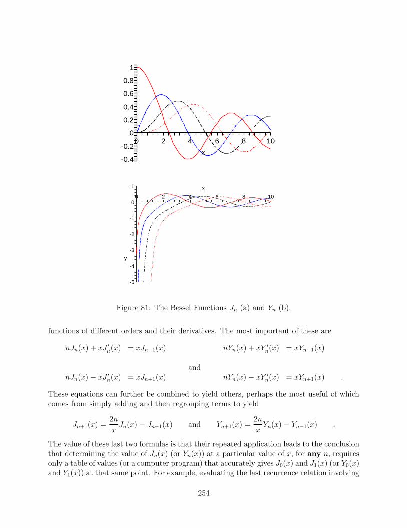
6

1

0.8

40

-0.4

2

x

80

0.2

0.6

-0.210

0.4

6420

y

1

0

-1

-2

-3

x

-4

-5

108

Figure 81: The Bessel Functions Jn (a) and Yn (b).

functions of different orders and their derivatives. The most important of these are

nJn(x) + xJ ′n(x) = xJn−1(x) nYn(x) + xY ′

n(x) = xYn−1(x)

andnJn(x)− xJ ′

n(x) = xJn+1(x) nYn(x)− xY ′n(x) = xYn+1(x) .

These equations can further be combined to yield others, perhaps the most useful of whichcomes from simply adding and then regrouping terms to yield

Jn+1(x) =2n

xJn(x)− Jn−1(x) and Yn+1(x) =

2n

xYn(x)− Yn−1(x) .

The value of these last two formulas is that their repeated application leads to the conclusionthat determining the value of Jn(x) (or Yn(x)) at a particular value of x, for any n, requiresonly a table of values (or a computer program) that accurately gives J0(x) and J1(x) (or Y0(x)and Y1(x)) at that same point. For example, evaluating the last recurrence relation involving

254

the ordinary Bessel functions for both n = 2 and n = 1 yields

J3(x) =4

xJ2(x)− J1(x)

J2(x) =2

xJ1(x)− J0(x)

,

which can be simplified (by eliminating J2(x)) to

J3(x) =(

8

x2− 1

)J1(x)− 4

xJ0(x) .

Unfortunately, from the point of view of realistic computations, there is at least one“minor” point we have glossed over. As we noted above, the series involved in the Besselfunctions converge at all values of x. However, the presence of the x2k+n term in these seriesdoes cause them to converge more slowly as the value of x increases. As a practical matterthen, these series are useful primarily when x is small. Therefore, mathematicians have de-voted significant efforts to develop simple expressions, commonly called asymptotic formulas,that give approximate values for the various Bessel functions - values that become more andmore accurate the larger x is. Perhaps the most widely used of these approximations are

Jn(x) ≈√

2

πxcos

(x− nπ

2− π

4

), x→∞ (7.2.5)

and

Yn(x) ≈√

2

πxsin

(x− nπ

2− π

4

), x→∞ . (7.2.6)

Note that both these two asymptotics confirm our earlier observation that the Bessel func-tions behave somewhat like decaying sinusoids. (They are however, and this is important,not equal to decaying sinusoids, since (7.2.5) and (7.2.6) are only approximate formulas.)

k J0(x) J1(x) J2(x) J3(x)1 2.4048 3.8317 5.1356 6.38022 5.5201 7.0156 8.4172 9.76103 8.6537 10.1735 11.6198 13.01524 11.7915 13.3237 14.7960 16.22355 14.9309 16.4706 17.9598 19.4094

Table 1: Roots of the Ordinary Bessel Functions of the First Kind - Jn

Before closing this section, there is one final important point we must make about thequalitative behavior of Bessel functions. As our earlier discussion and the asymptotic for-mulas (7.2.5)-(7.2.6) have indicated, the Bessel functions, like the sine and cosine, have an

255

k Y0(x) Y1(x) Y2(x) Y3(x)1 0.8936 2.1971 3.3842 4.52702 3.9577 5.4297 6.7938 8.09763 7.0861 8.5960 10.0235 11.39654 10.2223 11.7492 13.2100 14.62315 13.3611 14.8974 16.3790 17.8185

Table 2: Roots of the Ordinary Bessel Functions of the Second Kind - Yn

infinite number of distinct zeros. Nevertheless, there is a fundamental difference in the struc-ture of these zeros as opposed to the structure the zeros of trigonometric functions. Thisdifference is that the zeros of the Bessel functions are not evenly spaced along the axis,and there is no convenient formula, such as integer multiples of π, that exactly describesthem. The only way to express them is with a list or table. For example, Table 1 lists thefirst few zeros of the first three Jn(x) functions, while Table 7.2 lists the first few zeros ofthe first three Yn(x) functions. (In most practical applications, the zeros of the Yn(x) aregenerally not used as much as the zeros of the Jn(x)). However, the situation is not quite asbleak as the above discussion might at first seem. This is because the asymptotic formulasimply that for large x the kth zero (large k) of Jn(x) will approach

(n2

+ k − 14

)π, while the

kth zero of Yn(x) will approach(

n2

+ k − 34

)π. Therefore, once one decides with how much

accuracy they need to know the roots of a Bessel function, they can simply use tables untilthe asymptotic value agrees with the table value to the desired accuracy.)

7.3 Variants of Bessel’s Equation

Bessel functions appear frequently in applications, and especially in the solution of partialdifferential equations in cylindrical coordinates. In addition (and sometimes during thesolution of these same partial differential equations), several variants of Bessel’s equationvery frequently occur. Perhaps the most common of these variants is

x2y′′ + xy′ + (ξ2x2 − n2)y = 0 . (7.3.7)

In this equation, the change of variables s = ξx, including the application of the chain rule,e.g. dy

dx= dy

dsdsdx

= ξ dyds, reduces the differential equation to

s2d2y

ds2+ s

dy

ds+ (s2 − n2)y = 0 ,

which is clearly just Bessel’s equation of order n, but with s as the independent variableinstead of x. Therefore, the general solution to (7.3.7) can be represented

y(x) = c1Jn(ξx) + c2Yn(ξx) .

256

(It may help to view this last result as analogous to the fact that the general solution to

y′′ + y = 0 is y(x) = c1 sin(x) + c2 cos(x) ,

while the general solution to

y′′ + ξ2y = 0 is y(x) = c1 sin(ξx) + c2 cos(ξx) .)

A more impressive variant of Bessel’s equation is the general form

x2y′′ + [a + 2bxp] xy′ +[c+ dx2q + b(a+ p− 1)xp + b2x2p

]y = 0

where a, b, c, d, p and q are constants, which can be reduced to Bessel’s equation by a fairlytedious change of variables. We shall omit the details here, and simply present the resultinggeneral solution

y(x) = xαe−βxp

[c1Jν (λxq) + c2Yν (λxq)] ,

where

α =1− a

2, β =

b

p, , λ =

√d

q, and ν =

√(1− a)2 − 4c

2q.

One last fairly common variant of Bessel’s equation that we shall mention is the so-calledmodified Bessel’s equation

x2y′′ + xy′ − (x2 + n2)y = 0 . (7.3.8)

This equation can actually be viewed as nothing more than the special case (7.3.7) whichoccurs when ξ = j =

√−1. Its solution could therefore be written

y(x) = c1Jn(jx) + c2Yn(jx) .

This however, would be as awkward as writing the solution to

y′′ − y = 0 as y(x) = c1 sin(jx) + c2 cos(jx)

instead ofy(x) = d1e

x + d2e−x .

Therefore, the conventional way to represent the solution to (7.3.8) is by introducing twoadditional Bessel functions, denoted by In(x) and Kn(x), and commonly referred to as themodified Bessel functions of the first and second kinds, respectively. The general solutionto (7.3.8) is then represented

y(x) = c1In(x) + c2Kn(x) .

(Similarly, the solution tox2y′′ + xy′ − (ξ2x2 + n2)y = 0

is then representedy(x) = c1In(ξx) + c2Kn(ξx) .)

We shall not encounter the modified Bessel functions in this text, and simply refer the inter-ested reader to Abramowitz and Stegun, or Spanier and Oldham for a complete discussion.

257

PROBLEMSUse Bessel Functions (the big ugly equation) to find the general solution to each ODE

below.

1.x2y′′ + 3 xy′ +

(−3 + 4 x4

)y = 0

2.x2y′′ +

(x+ 2 x2

)y′ +

(−4 + 9 x−2 + x+ x2

)y = 0

3.x2y′′ − 5 xy′ +

(9 + 4 x2

)y = 0

4.x2y′′ +

(x− 2 x3

)y′ +

(−1/4 + x−2 − 2 x2 + x4

)y = 0

Answers

1.y(x) = AJ1(x

2)/x+ B Y1(x2)/x

2.y(x) = e−x (AJ2(3/x) +B Y2(3/x))

3.y(x) = x3 (AJ0(2x) +B Y0(2x))

4.y(x) = ex2/2

(AJ1/2(1/x) +B Y1/2(1/x)

)

258

References

Abramowitz, M., and Stegun, I., Handbook of Mathematical Functions, Dover Pub. Co. NewYork, 1965.

Boyce, W. E. and DiPrima, R. C., Elementary Differential Equations and Boundary ValueProblems, Fifth Edition, John Wiley & Sons, New York, 1992.

Spanier, J. and Oldham, K. B., An Atlas of Functions, Hemisphere Pub. Co., New York,1987.

259

Index

amplitude, 49amplitude distortion, 64Amplitude Spectrum, 188argument, 188asymptotic formulas, 255

Bessel Function, 252Bessel functions, 165, 253Bessel’s Equation, 251Bessel’s equation, 165, 257best mean square approximation, 51boundary conditions, 76

causal function, 191circular membrane, 159completeness, 128complex exponential form, 53convergence tests, 13

D’Alembert solution, 138, 143delay, 48delta function, 185digital signal processing, 60Dirichlet, 76, 141dispersion, 66

eigenfunctions, 90, 101eigenvalues, 90, 101Euler’s constant, 253even function, 35

First Kind, 252first kind, 77fixed end, 76, 85Fourier, vFourier coefficients, 28Fourier integral transform, 183Fourier series, 25Fourier transform, 183free end, 77, 78Frequency domain, 154, 170frequency domain, 159fundamental frequency, 133

harmonics, 134

improper integral, 7impulse function, 203infinite series, 11initial conditions, 82

inverse Fourier transform, 183

L’Hopital’s rule, 7Laplace transform, 183Laplacian, 147limit, 5linearity, 195

magnitude, 188mean square measure, 42mean-square convergence, 44membrane, 147method of Frobenius, 251mixed end, 80, 106modes, 134, 155, 170modified Bessel functions, 257modified Bessel’s equation, 257

natural frequencies, 133, 171natural frequency, 155Neumann, 78, 97

odd function, 35order notation, 8, 10orthogonality, 125, 153, 167Orthogonality Integrals, 26

Parseval’s Theorem, 49phase angle, 48phase distortion, 64Phase Spectrum, 188piecewise continuous, 32piecewise smooth, 32plane wave, 159pointwise convergence, 19, 20polar coordinates, 147power series, 251

recurrence formulas, 253reduction of order, 252regular Sturm-Liouville, 121Riemann sum, 180rigid edge, 148Robin, 80

scaling, 196second kind, 78, 252separation of variables, 86, 148sequences, 4shifting, 198

260

sifting property, 204sinc function, 186singular Sturm-Liouville, 164spectrum, 49, 171square pulse, 185Sturm-Liouville, 119, 151

third kind, 80Time domain, 158, 172time domain, 159transform of the derivative, 200transform of the integral, 202

uniform convergence, 21, 41unit impulse, 185unit step, 211

Weierstrass, 22Weierstrass M-test, 22Weirstrauss M-test, 67

Zeno’s paradox, 1

261