www.sciencemag.org/cgi/content/full/334/6062/1578/DC1

Supporting Online Material for

Uninformed Individuals Promote Democratic Consensus in Animal Groups

Iain D. Couzin,* Christos C. Ioannou, Güven Demirel, Thilo Gross, Colin J. Torney, Andrew Hartnett, Larissa Conradt, Simon A. Levin, Naomi E. Leonard

*To whom correspondence should be addressed. E-mail: icouzin@princeton.edu

Published 16 December 2011, Science 334, 1578 (2011)

DOI: 10.1126/science.1210280

This PDF file includes:

Materials and Methods SOM Text Figs. S1 to S12 Table S1 Full Reference List

Other Supporting Online Material for this manuscript includes the following: All code and data are available online at: http://icouzin.princeton.edu/uninformed-individuals-promote-democratic-consensus-in-animal-groups/

2

Materials and Methods 1. Spatial model

We adapt the model of Couzin et al. (5). This is a deliberately generic and minimal spatial model for the study of collective dynamics in animal groups. Both social interactions and goal-directed behavior are included. In this version of the model the parameter represents knowledge of and/or preference for specific target locations, as opposed to fixed directions (5,13,24). This allows us to determine which target is reached in each realization of the simulation, and also allows us to relate more directly to experimental tests (see below).

Targets were set at; x = 100, y = -50 for target 1, arbitrarily preferred by the majority, and x = 100, y = 50 for target 2 preferred by the minority, unless otherwise indicated. Individuals started at random positions and random orientations within a box 2 by 2 units, centered at x = 0, y = 0. The group typically initially expands and become dynamically stable within a transient period of approximately 200 time steps after which the group was re-centered on 0, 0 so that starting conditions are independent of any initial drift. The group was then allowed to approach the targets. When the group centroid reached within 4 units (body lengths) of either target the choice was recorded. Unless otherwise stated, 20,000 replicates were then conducted for each set of parameter values (e.g. for each combination of N1, N2, N3, 1 and 2) to calculate the relationship between those parameters and the probability of choosing the majority-preferred or minority-preferred target. Under most parameter conditions groups rarely split (see Fig. S5). 2. Adaptive network model

We develop an analytically tractable model based on adaptive-networks (AN), inspired by a voter model (25). While the proposed AN model is non-spatial and employs discrete opinions, it captures the two main ingredients of the spatial model: First, the tendency of individuals to adopt the opinion of others in their local (in the AN topological) neighborhood, which leads to a positive feedback reinforcing the predominant opinion. And, second, intransigence of the informed subpopulation. Whereas intransigence is directly implemented in both models, reinforcement and positive feedback arises as an emergent property in the spatial model, but is deliberately incorporated into the AN model. The simplified approach taken in the AN model complements the spatial model by allowing a cleaner analysis and a direct control of the involved processes.

The adaptive network (AN) model builds on a modeling approach proposed by Huepe et al. (17). The basic idea of this approach is to capture the key aspects of the topology of the interactions (i.e. who perceives whom) without accounting in detail for the geometry (i.e. who is where). For this purpose we employ tools from network science and describe the system as a set of nodes and edges. The nodes correspond to individuals, whereas a link (edge) between two nodes indicates mutual awareness between the corresponding individuals.

Each node has an internal state indicating its current opinion. Following Ref. (17) we assume that the current opinion of an individual is a discrete (Boolean) variable, which can take

model. Going beyond Ref. (17) we also assign to each individual a fixed informational status, which is either right-informed (the individual has a preference for, or a knowledge of, the right target), left-informed (the individual has a preference for, or knowledge of, the left target) or

3

uninformed (the individual is unaware of either target or has no preference). In contrast to the current opinion, the informational status does not change in time. In the following we assume that the number of right-informed individuals is larger than the number of left-informed

The network model evolves in time according to simple heuristic rules designed to capture

b) the change of the topology due to individuals encountering and separating from one another. Although the model is defined in detail below, let us point out some specific assumptions

that have been made in the model set-up. Regarding a) we assume that opinions change mainly due to interactions with other individuals. An individual that is linked to one or more individuals holding the opposite opinion has a probability of adopting this opinion. This probability is nonlinear, such that being in contact with multiple individuals holding the opposing opinion induces a higher average rate of opinion change than the sum of the rates induced by the opposing individuals on their own.

In addition to opinion changes induced by neighbors, we assume that the individuals have a small spontaneous probability of changing their opinion. In the AN model spontaneous opinion changes are used to capture the effect of informational status: informed individuals have an increased probability of spontaneously switching to the opinion they are informed about; further, the increased spontaneous switching probability is used to model the difference in intransigence between the majority and minority subpopulations. We model a situation where the minority is has a stronger preference than the majority by setting the average rate at which a left-informed (minority) individual -

We note that the implementation of intransigence in the AN model differs significantly

from the spatial model. For typical parameter values the Boolean switches in the AN model cause a higher level of stochastic fluctuations than the noise in the spatial model. We compensate for this by considering a larger number of individuals in the AN simulations.

Regarding b), ththat the network in the model is not embedded in space. In other words the AN model does not keep track of the spatial position of individuals. Therefore, all rules for the creation and deletion of links must depend solely on the opinion states of the nodes. We can think of individuals with different opinion states as moving in different directions, therefore individuals rapidly encounter and leave (create and delete links) with individuals of the opposite opinion. Conversely we assume that individuals move alongside other individuals with the same opinion for prolonged periods of time, resulting in both lower creation and deletion rates. A detailed description of this model and analysis is given in SOM Text, below. 3. Convention model

This model is based on a convention game, as described in (27) and used to describe self-enforcing normative behavior in social and economic systems.

Originally this simple model was proposed as an aid in the study of the evolution of conventions or social norms, and is relevant to situations where it is desirable to adopt the same strategy as the majority of the population. Examples of these situations from a social or economic standpoint are, the adoption of a novel technology, the carrying of a particular

4

currency, or the decision of whether to drive on the left or right of a highway; once a significant portion of the population have adopted a given strategy, it becomes costly to adopt an opposing position.

In its simplest form the model is presented as a currency game. We present the basic model here, as originally described in (27). Imagine there are two forms of currency; gold and silver. Each individual within the population must decide which currency to carry, and will only be able to trade with those who carry the same currency. The model is simulated as follows. At each timestep an individual is selected at random from a population of size N. This individual then observes the population and switches to the currency held by the majority of individuals. To introduce a stochastic element this occurs with probability 1- , and with probability a random currency is selected.

The macroscopic behavior of this form of the model is long periods of stasis, in which one currency dominates and is held universally, punctuated by noise-induced transitions where the system switches collectively to the opposite state. Further extensions to this model include incorporating an inherent bias so that all individuals intrinsically prefer a particular state, and restricting the observation of the current consensus to an estimate based on a subsample of the population. For further analysis of the model see (27).

To address the role of uninformed individuals in consensus decision-making in this parsimonious framework we modify the convention model to include a limited sampling of the population and introduce individual level preferences for a given outcome, manifested through a reduced probability to switch to a non-preferred state. The model therefore has several fundamental properties in common with both the adaptive network model and the spatial model.

als to estimates of the current consensus we approximate the local neighborhood in our previous models in the well mixed or low viscosity limit.

Since switching is based on multiple samples, there is a nonlinear relation between the proportion of individuals currently in a given state and the probability to switch to that state. This results in positive reinforcement of collective decisions and, in the absence of explicit noise, rapid transitions to complete consensus. This nonlinearity is an emergent property of the spatial model, but is introduced here in a more explicit fashion. 4. Experiment with schooling fish

Golden shiners (Notemigonus crysoleucas) were supplied by a commercial live bait supplier (Anderson Minnow Farm, Arkansas, U.S.A.) and were kept under laboratory conditions for at least 3 months before the start of the experiment. Water temperature was maintained at 16°C and with a 13:11 day:night light cycle throughout this period and the experiment. 27 gallon black plastic stock tanks housed the fish, with approximately 120 fish per tank, and were fed 3 times daily with tropical flake food.

90 fish (47.6 ± 3.3mm mean ± s.d. standard body length) were given a dorsal epidermal tag (Visible Implant Elastomer; Northwest Marine Technology) in one of two colors (45 fish per color). After 48 hours, they were moved to the main experimental arena (Fig. S3), fed, then allowed to habituate overnight. The door to the start chamber was left open during this time. Fish were then moved into either holding compartment T1 or T2 (Fig. S3), split by tag color.

The training procedure was as follows. One of the two groups of fish, i.e. that currently housed in either compartment T1 or T2, was randomly chosen. Approximately 0.03g of tropical

5

flakes were finely crushed, suspended in water and pipetted into the 8.6cm diameter Petri dish assigned as the target for these fish (Fig. S3). A subgroup of 15 fish from this compartment was then haphazardly netted to the release chamber (R in Fig. S3). After 5 minutes habituation, the door was raised remotely, allowing the fish to enter the main arena and find the food. A Sony PMWEX1R camcorder filmed the entire tank at 30fps. After all the food reward was consumed, the training session was ended. These fish were then returned to the start chamber and the training procedure repeated. After a third training, the fish were returned to their home compartment. Transparent plastic barriers (thin dotted lines in Fig. S3) were used to partition the holding compartments to separate fish already trained that day from those yet to be trained.

Training took place alternately between the two compartments (in subgroups of 12-15 fish; reasoning for this variation in group size is given below) until all fish had completed the training procedure. After training, the transparent barriers were removed. Fish in both compartments were then fed a standardised amount of crushed flake food (approximately 0.65ml), and then again at the end of the day.

This training protocol was carried out daily for seven days. To minimize any difference in training to the two different targets, if training was started with a subgroup from compartment T1 on one day, we started training with fish from compartment T2 the following day. Any fish that lost body condition at any point were removed and not used again (7 from those trained to the blue target and 12 from those trained to the yellow target across the whole training/testing period; from 135 in total for each). This necessary procedure combined with the fact that we wanted to train each fish only once per day, resulted in training groups being between 12 and 15 fish. On the second to seventh days, testing was carried out (always >1 hour after the fish were fed post-training). This followed the same procedure as training with the following exceptions. For each trial, 6 fish from one trained group (the majority) and 5 from the other (the minority) were moved to the start chamber with either 0, 5 or 10 naive fish from a stock tank (the experimental treatment). The treatments were ordered using a complete random block: of the 6 trials carried out each day, each treatment appeared once in the first 3 trials, and then once again in the following 3 trials. Within each block of 3 trials, the treatment order was randomised. Which group of fish (from A or B) formed the majority was also randomly determined, with the restriction that half of the trials within each treatment would use fish from A as the majority, and the other half those from B. Trained fish were used in a trial only once per day, with tested fish kept separate from untested fish with the transparent barriers. The colored elastomer tags facilitated separation of the two groups of trained fish. A single stock tank provided all naive fish on a day of testing. Stock tanks were used sequentially between days, so that any one naive fish could not be used as a naive fish more than once every four days. There was no food present during these trials, so naive fish never experienced a food reward in the test tank and trained fish never found food in a dish they were not trained to. Trained fish always underwent another training session with food at their trained target before testing the next day.

This method was repeated 3 times altogether, each time training a different set of inexperienced fish to become informed (Fig. S4). In total, 108 trials were carried out, balanced between these three sets of informed fish (36 trials each), the number of trials per treatment (36 trials each), and which target was the majority target (56 trials each).

The first target reached by any fish (the head being within 2 body lengths (bl) of the nearest edge of the dish) was recorded as the decision made by the shoal. The first arrival to a dish was used as the criterion since the lack of feeding by the first fish provided feedback to the others as

6

to the absence of food, thus altering their propensity to continue towards the target. Videos were analysed partially blind since the target the majority was trained to was unknown. Furthermore the experimentalist (C.C.I.) was blind to the theoretical predictions.

Binomial Generalised Linear Models (GLMs) were used to analyse the effect of the number A

polynomial effect of this variable was included since visual inspection of the data suggested such a relationship when the majority was trained to the y

also included as variables. The degree of training per testing day was quantified as the time taken to reach the target (as in Fig. S4), averaged across the three replicate trainings per session per subgroup, averaged across the 3 subgroups, then averaged between the groups trained to the two targets. The model began as fully-factorial to examine whether any of these effects were inter-dependent (i.e. significant interaction terms). In two further tests, data were split by which target the majority were trained to, and the effect of the number of naive individuals on reaching the majority target was assessed for each.

Analyses of the training data also tested for the pre-existing bias towards the yellow target. Two response variables were used to assess the degree of training and were analyzed separately: the time taken to reach the correct (rewarding) target, and whether this was the first target reached first. Negative binomially and quasibinomially distributed GLMs were used, respectively, with the target, the number of days of training and which of the 3 (1st, 2nd or 3rd) replicate trainings it was as explanatory variables.

Higher-order interaction terms were removed where non-significant. All statistical analyses were carried out in R 2.10.1. All experimental work was carried out in accordance with federal

Care and Use Committee.

7

SO M T ext 1.1 Details of the spatial model

Groups are composed of N individuals, each represented at time t by a position and unit direction vector . Individuals modify their motion based on the orientations (heading) and/or positions of others j within two zones. In the smaller zone, with radius centered on the focal individual, the repulsion rule applies, defined as turning away from individuals within this range

-­‐ -­‐-­‐

Equation 1

subsequent time step. In this, and the following equation, the denominators are simply normalizing factors.

To represent the observed behavioral tendency for individuals in groups to maintain personal space in groups, including the species of fish we use here for our experiments (16), avoidance takes precedence over the other behavioral rules. If there are no individuals in the repulsion zone, however, the focal individual exhibits attraction towards, and alignment with the direction of travel of, neighbors j within radius

Equation 2

In addition to these social interaction rules, individuals may have a preferred direction of travel . They reconcile social and goal oriented tendencies with a continuous weighting term,

i

Equation 3

their desired direction of travel being unit vector . If = 0 individuals either have no desire to move in a preferred direction or are

uninformed/naïve. If an individual s approaches 1, it tends to equally bias its tendency to move in its preferred direction with social interactions. As exceeds 1, individuals are more heavily influenced by their preferred direction than by their neighbors. Since there are two competing groups in the present model we define 1 and 2 as the preference strengths of informed subsets N1 and N2, respectively.

In the present model the term represents knowledge of and/or preference for specific target locations, as opposed to fixed directions in (5,13,24). Consequently the directional component is a unit vector directed from individual i to its preferred target and thus changes as individuals move through space.

A further (minor) difference from (5) is that here t = 0.1s (previously, due to computational constraints, it was set to 0.2s). Individual motion is subject to random influences. This is simulated by rotating by a random angle taken from a circular-wrapped Gaussian distribution, centered on 0, with a standard deviation of = 0.01 radians. Individuals may not be capable of instantaneously adopting their desired direction, depending on their turning rate . In the standard model values are based on an estimate of typical turning rate in

8

fish = 2 rad (5). Speed = 1, range of repulsion = 1 (body length) and, unless otherwise indicated, maximum range of social influence = 6 (5,16).

Due to the intensive computation required the simulation was coded in the NVIDIA Compute Unified Device Architecture (CUDA), a C-like language for Generally Programmable Graphics Processing Units (GPGPU) and computed on multiple NVIDIA Tesla C1060 high performance computing boards (each with 240 scalar processors). 1.2 Simplified scenario and phase space analysis of the spatial model

In order to reveal the underlying mechanism in our spatial model we created a simplified geometry that facilitates investigation of long-term dynamics and also, due to its geometrical symmetry, an investigation of the role of stochastic fluctuations. This model is exactly the same as that described in 1.1 with the exception that the preferred targets are replaced by preferred directions, 180° apart (i.e. infinitely distant targets). Arbitrarily the majority-preferred direction is defined as along the positive x-axis and the minority-preferred direction along the negative x-axis. Since the preferred directions are in a single dimension we can define the order of each of the informed subsets (N1 and N2) and the uninformed subset (N3) as   where

j (1,2,3) and is the x component of the velocity of individual i at time t. This value therefore represents, for each subset, a continuum from strong alignment (conformity) with the minority opinion ( -1), with the majority opinion (0. An important advantage over considering the mean heading of each subset is that direction becomes indefinable as the system tends towards disorder (since the length of a summed heading vector of a disorganized system approaches 0).

Representing the degree of conformity between informed subgroups as the absolute difference between N1(t), N2(t) and N3(t) we find, using a large number of simulations that the uninformed population N3 tends to be undiscerning with respect to adopting, or being biased towards, the N1 and N2 for relatively small differences in abs( N1 - N2), but exhibit a bias towards the majority for relatively large differences between N1 and N2, where the degree of coordination is defined as ½(abs( N1 N3) - abs( N2 N3)) (Fig. S6).

of disorder result in uninformed individuals being more likely to experience a bias in the spatial distribution of their neighbors (due to the tendency for informed subsets to aggregate at their respective leading edge of the group) and thus, probabilistically be attracted towards the true numerical majority. This is a very noisy process, as evident from Fig. S6a where it can be seen that uninformed individuals also frequently side with the minority.

Stochastic fluctuations are inevitable in such groups. Typically they are damped, but they can, through ergodic random effects, accumulate to disrupt the coherence of individual interactions over long length-scales. If a minority-preferred direction is selected, stochastic processes can aid in escaping this choice. This is because, as shown in Fig. S6b, uninformed individuals tend to preferentially reinforce the majority-preferred direction when stochastic fluctuations result in substantial turning, or disorder. Consequently if traveling in the minority-preferred direction large fluctuations tend to be amplified by uninformed individuals causing the group to transition to the majority-preferred direction. Exactly the same process results in the uninformed individuals spontaneously stabilizing the majority-preferred direction since large fluctuations tend to facilitate reinforcement, and thus stabilization, of the majority preference.

9

Consequently if the distance between the targets is increased the role of uninformed is emphasized (Fig. S7a). As long as the minority individuals are not sufficiently intransigent and there is a sufficient numerical majority the behavior of uninformed individuals will result in the majority-preferred direction being more (dynamically) stable than that of the minority (Fig. S7b). However if 2/ 1 is very high and there is a low N1/N2 ratio, the minority will dictate group motion regardless of uninformed individuals, as shown in Fig. S7c (c.f. Fig. 2c in main text). 1.3 Features of this model that determine the group-level behavior

Our analysis of the spatial model suggests the importance of the following features: a) Individuals can influence, and are influenced by, others with whom they interact - they

tend to adopt (probabilistically) the opinion they perceive to be the local majority. This results in positive feedback and results in ordered states (of the collective) being inherently more stable (Figs. S6, S7b) than disordered states. Consequently if groups become disordered (such as through stochastic influence) they rapidly regain order (5,13,17,24).

b) The strength of individual preference manifests as intransigence during interactions with others. A sufficiently intransigent minority can overcompensate for the numerical advantage of a majority.

c) Since they exhibit little intransigence or intrinsic bias uninformed individuals lend support to what they perceive (locally) as the numerical majority. A relatively small change in their number can dramatically alter the outcome of consensus decisions.

It is hard to determine from analyzing this model alone whether the continuous decision space can be reduced to a binary opinion state, or whether the spatial relation between individuals is essential, and thus whether our results are likely to be generalizable to other systems. However identification of the essential aspects allows us to create reduced representations (the adaptive network model and convention model).

10

2.1 Details of the adaptive network model

We consider a network of N    nodes, which is initialized with as an Erdös-Renyí random graph with mean degree 10. Informational status is assigned such that the number of right-informed (majority) nodes is N1, the number of left-informed (minority) nodes is N2, and the number of uninformed nodes is N3. The nodes have an internal Boolean degree of freedom denoting their current opinion (Right/Left) that is initialized in agreement with the informational status for the informed nodes and assigned randomly with equal probability for the uninformed nodes.

In the following we denote the informational state of a node with the lower case letters r, l, and u respectively, whereas the current opinion is denoted by the upper case letters R and L.

In the following we formulate the dynamics of the model in terms of transition probabilities in a sufficiently small unit time step. We emphasize that these probabilities should be read as defining the corresponding average rate of stochastic events. The network simulations reported in the paper use an event-driven algorithm, which provides a very close match with continuous time dynamics and does not use a discrete time step. Using this algorithm the network is updated as follows:

Induced opinion changes: A given focal individual changes its opinion with probability c for every individual of opposing opinion it is linked to. To capture the nonlinearity of induced response, there is an additional probability p  of switching for every pair of opposing individuals with whom the focal individual interacts (is linked to).

Spontaneous opinion changes: A given uninformed individual switches its state spontaneously with probability q. A left-informed (minority) individual has a probability q  of switching to state R when in state L, but a higher probability WL of switching to state L when in state R. Likewise a right-informed (majority) individual has a probability q  of switching to state L when in state R, but a higher probability WR of switching to state R when in state L. We consider the case WL >WR, which models the stronger preference of the minority and is thus analogous to the intransigence in the spatial model.

Encounters: For every pair of individuals that are not linked and hold opposing opinions there is a probability ao that the individuals encounter each other and a link is established. Similarly, for every pair of individuals that are not linked and hold the same opinion and there is a probability ae that a link is established between the individuals (ao>  ae).

Losing contact: For every link between individuals holding opposing opinions there is a probability do  that the link is broken. Similarly for every link connecting individuals holding the same opinion, there is a probability de that the link is broken (do>de).

Unless otherwise stated (see Fig. 2c) we use the following parameter values ao = 0.70, do = 0.25, ae = 0.20, de = 0.10, q = 0.05, WL = 0.80, WR = 0.20, c = 0.10, p = 0.20, N1/N2 = 1.25, N = 10000. 2.2 Analytical description of the adaptive network model

From the adaptive-network model analytical results can be obtained by a moment expansion (17). The idea of this expansion is to write differential equations that capture the abundances of a set of small subgraphs in the network.

11

In the following we denote the density of nodes with opinion and information as . Further, we denote the density of links between nodes of given type A and B

as ; the density of connected triplets consisting of nodes of type A, B, and C as ; and the density of start motifs consisting of a node of type A connected to three nodes of type B, C , and D as (where for clarity we used A, B, C , and D as placeholders for symbols of the form ).

We start by writing an equation that capturing the dynamics of number nodes holding opinion R and having an informational state . This yields

Equation 4

where , . The terms

in this equation capture gain from spontaneous switching, loss from spontaneous switching, and the linear and nonlinear part of the induced opinion changes respectively. The corresponding equation for can be obtained by replacing all instances of L by R and vice versa.

The equation above is dependent on the number of larger sub-graphs. We therefore write the corresponding differential equations

Equation 5

Equation 6

where , is the Kronecker delta function, is the multiplicity of subgraph in graph .

We could continue by writing differential equations governing the larger sub-graphs appearing in Eqs. 5 and 6. However, this would yield complicated expressions containing even larger sub-graphs. We therefore terminate the expansion at this point by a moment-closure approximation approximating the density of larger sub-graphs as

12

Equation 7

Equation 8

where and .

The specific moment-closure approximation used above is a pair approximation. The validity of this approximation depends on the absence of correlations longer than a single link. Although this assumption is certainly not met exactly, the pair approximation is known to yield good results in adaptive network models including the model by Huepe et al. (17). In the present model the validity of the approximation can be verified by a comparison with network simulations such as shown in Fig. 2b.

By the pair approximation we obtain a closed system of differential equations, describing the time evolution of different types of nodes and links in the network. This system thereby constitutes an emergent-level description of the network dynamics and can be studied by the full range of tools available for analyzing systems of ordinary differential equations. 2.3 Dynamical mechanism of the adaptive network model

In comparison to the spatial model the AN model describes the dynamics in a substantially simplified and abstracted form. Nevertheless the AN model is still capable of capturing the main properties of the dynamics (see Fig. 2). The similarity of the dynamical behavior of the two models strongly suggests the same underlying mechanism (compare for instance Figs. 2c and S7c). By reproducing these dynamics while neglecting much of the biological complexity, the AN model can identify those properties that are essential for the observed behavior. We emphasize that the embedding in physical space, although known to be of importance in many ecological systems (26), is not among these characteristics.

The essential features that are required for reproducing the observed dynamics are, first, a (nonlinear) propensity of individuals to adopt the opinion of their topological neighbors, and, second, a mechanism of intransigence that biases informed individuals to a certain preferred opinion. The observed return of control can be explained by the interplay of two dynamical processes; the direct interaction between informed individuals and the indirect interaction through uninformed intermediaries. To understand how the control is returned, consider that the propensity to adopt the opinion of others introduces a positive feedback. Uninformed individuals contribute to this feedback without adding to the bias in the system. Thus adding uninformed individuals has a stabilizing effect on both majority-preferred and minority-preferred states. In the parameter range under consideration, the minority-preferred state is stable even without addition of uninformed individuals, and thus does not profit from the addition of uninformed individuals. By contrast, the majority preferred state is infeasible without uninformed individuals, but emerges once a certain density of uninformed individuals is reached. When sufficiently many uninformed are present, the system is in a bistable regime where both the minority-preferred state and the majority-preferred state are feasible. Our results show that in this state the numerical advantage of the majority can overcome the stronger intransigence of the minority. We note that in a stochastic agent-based system there are nevertheless episodes in which the system switches to the minority-preferred state.

13

3.1 Details of the convention model

If we introduce individual-level preferences as asymmetric switching probabilities (as in the AN model), the dynamic of the decision process is described as follows. At each timestep one individual, i, is selected at random from a population of size N. If i is informed and in its preferred state, then it is left in this state with a probability determined by the strength of its preference (acting analogous to in the spatial model). However if an individual does not remain in its current state due to its inherent bias, it will make S observations of the population opinion, drawing at random with replacement and including the possibility of selecting itself. Individual i then changes its state to the most popular (majority) opinion within its sample. In the event of a tie the opinion selected is randomly assigned. Results from numerical simulations of this algorithm are shown in Fig. S8, for the case of a 6:5 ratio in majority to minority preference, with the system size increasing but this ratio held constant.

It should be noted that S can be greater than N since sampling occurs with replacement, and should not be considered simply as the range of perception of the individual but rather as related to the level of individual noise (error) when an individual attempts to assess the consensus. For example, this could be due to observational constraints, cognitive limitations, the presence of random fluctuations in the behavior of others etc. 3.2 Analytical approximation of the convention model

We begin with three populations, N1, N2 and N3 representing the informed majority, informed minority and uninformed individuals, respectively. Without loss of generality we define p(t) as the fraction of the population in the majority-preferred state at time t. Similarly p1(t) is the proportion of the N1 population in this state, p2(t) the proportion of N2 individuals etc.

Next we define T(x) as the probability, per unit time, of switching to a state given that the proportion x of the population are currently in that state, and determines the strength of an

influence. For the uninformed and their likelihood of switching into a state depends only on the number of individuals in that state. However if individuals have a preference, , and therefore a biased individual in its preferred state will less readily switch. Transition probabilities for the informed groups are asymmetric by definition. We label the level of bias for individuals in populations N1 and N2, and respectively. As the probability that an individual will switch away from its preference tends to zero as the opinion strength increases, and is 1 for an unbiased (uninformed) individual, it may be considered equivalent to where is the preference weighting of the spatial model.

In the limit of large N, the dynamics are determined by

Equation 9

Equation 10

Equation 11

14

where T(p) is the probability that an unbiased individual will switch to the majority preferred state given the total proportion, p, of individuals in this state. The transition probability is found via the binomial distribution

Equation 12

where X is the number of observed individuals in the majority-preferred state.

We can employ the normal approximation of the binomial distribution to find the probability that X > 0.5S, to give

Equation 13

and

Equation 14

where erf is the error function, and the 50% tie break rule has removed the need for a continuity correction.

By Taylor expanding the discrete time update equation, introducing the above expression for T(p), and taking the limit , we obtain a continuous system of ordinary differential equations which define the time-evolution of the system,

Equation 15

Equation 16

Equation 17

where

For initial conditions we assume ; individuals begin in their preferred state with naïve individuals randomly assigned. Fig. S9 shows the time evolution of the system of ODEs illustrating the qualitatively different behavior when uninformed individuals are introduced (the only distinction between (a) and (b) being the addition of an uninformed sub-population).

Although a closed form solution to this system of equations has not been attained, a useful and informative quantity is the rate of change of the proportion of individuals in each state at time t = 0. Numerical simulations show this is a good proxy for the ultimate final state of the system, i.e. if the proportion of the population p in the majority-preferred state is decreasing it is likely to continue doing so and the minority will ultimately win (see Fig. S8).

15

An expression for this quantity can be found as

Equation 18 and the sign of this quantity is positive (the majority opinion receives a net influx of

individuals), if

Equation 19

Some informative limits for this inequality are;

As (corresponding to a large number of uninformed individuals), , hence neither opinion is favored at the onset and there is only a slight advantage to the majority-preferred opinion due to the initial conditions. In this situation the probability of each outcome tends to .

If there are no uninformed individuals, as the right side of the inequality tends to one, therefore the majority opinion will always be decreasing at t = 0, since the error function is bounded by [-1,1].

For , as , meaning the value of p is known perfectly, the left hand side of the inequality approaches unity, and since the right hand side is strictly less than one, the minority-preferred state will always be decreasing at the outset.

Uninformed individuals tend to align with the perceived numerical majority and reinforce the majority preference before the minority are able to control the decision. Given sufficient uninformed, the new majority group (majority individuals + aligned uninformed) becomes stable enough not only to resist the influence of minority individuals but to exert enough social influence to force them towards the majority-preferred side.

This final model demonstrates that spatial or topological structure of interactions is not necessarily an essential requirement in order for uninformed individuals to significantly alter collective decision-making. The macroscopic, self-reinforcing behavior the topology generates is required, however, allowing us to recover an equivalent result in a model where the positive reinforcement of consensus is explicitly introduced.

16

4.1 Bias towards the yellow target in our experiments with schooling fish The behavioral response of trained fish in our trials (see the data point corresponding to no

uninformed individuals in Fig. 3) suggests a bias exists in favor of the yellow target. Biases for color and/or brightness of stimuli have been found to occur for sensing and processing pathways in fish and other animals. Innate color preferences can sometimes reflect ecologically-relevant stimuli, but this is not always the case (20). Detecting the basis of such a bias is complex (see (20)) and beyond the scope of the present study.

When trained to that target the minority had a sufficiently strong preference to dominate the decision-making process, provided there were no untrained individuals. As would be expected, when the majority was trained to the yellow target the group exhibited a preference for that target irrespective of the number of untrained individuals.

This bias was also evident in the training of the fish. Those trained to the yellow target were on average faster to reach their target (Fig. S4) and more likely to reach this target first (Fig. S10) compared to fish trained to the blue target. When considering the learning curves shown in Fig. S4 and Fig. S10, there was only weak statistical evidence that fish trained to the blue target

to the yellow target as training progressed, although visually the learning curves for the blue target do appear steeper. The lack of a significant interaction is likely to be because learning occurs in the same direction regardless of target (the correct target is more likely to be reached first and reached more quickly); to find a significant difference between two such gradients (i.e. the interaction) would require a very large effect or sample size. Although there was no statistical difference in learning rates, when fish trained to the yellow and blue targets were tested together in the trials, the relative bias toward the yellow target did statistically reduce as the fish became more trained (Fig. S11). Whether fish trained to the blue target were in the majority or minority, they were more likely to reach their preferred target as training progressed. Correspondingly, fish trained to the yellow target were less likely to do so. As these trends are in opposite directions (increasing and decreasing, respectively), a significant interaction between the degree of training and the majority target was found (Table S1 and Fig. S11). This change in the relative bias between the two targets as the experiments progressed was not affected by the number of untrained individuals in the shoal; this is apparent both statistically (the non-significant three-way interaction in Table S1) and visually (the 3 fitted curves for each target in Fig. S11 are all of similar gradients). In other words, the amount of training (within the range tested) did not affect the relationship between the naive individuals and which target was favored by the majority.

It is possible that this bias reflects an intrinsic bias. Typically researchers take great pains to exclude biases in experiments, but here we took advantage of a bias in the context of collective decision-making. If really intrinsic, and thus present without training, this may affect our assumption that uninformed individuals exhibit no preference during our experiments. However

opposite effect to the one we found; namely adding untrained individuals should have enhanced the minority preference for the yellow target, not the majority preference for the blue target. Consequently if untrained individuals did exhibit a bias to the yellow target it was not substantial enough to counterbalance the phenomena we reveal here whereby they promote the majority preference.

Post hoc analysis of our spatial model supports the validity of this logic. In Fig. S12a we

17

can result in substantial target preference. However, when we introduce such a biased N3 population into our simulations we still find that they tend to return support to the majority-preferred target (Fig. S12b). If this bias increases substantially these individuals would no longer be sufficiently naïve and thus eventually would act like an informed subpopulation (in this example favoring the minority opinion).

18

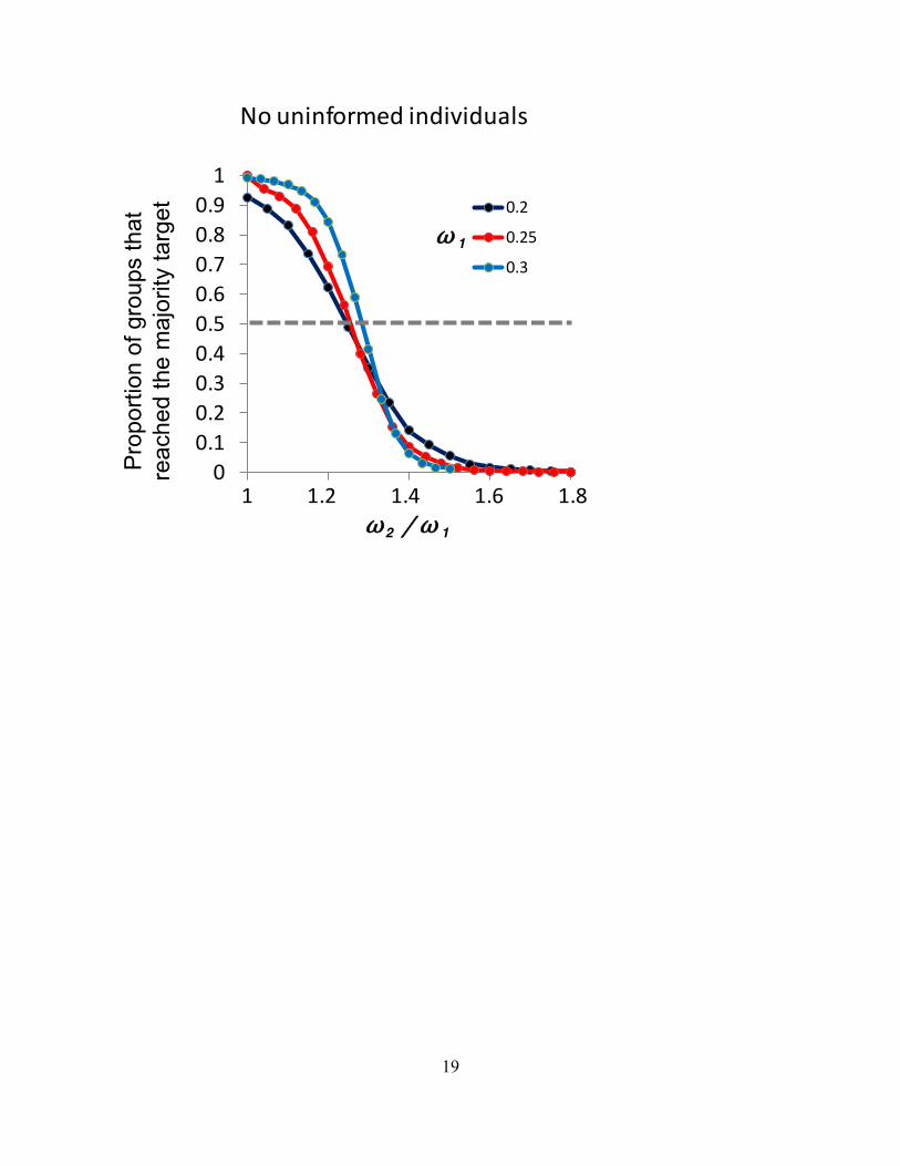
F ig. S1 When there are no uninformed individuals the numerical minority can increase 2 to exert control over the consensus decision. All other parameters are as for Fig. 1b. 20,000 replicates per data point.

19

0

0.1

0.2

0.3

0.4

0.5

0.6

0.7

0.8

0.9

1

0 0.2 0.4 0.6 0.8

0.2

0.25

0.3

maj

min =   . maj

Probab

ility  of  reaching  

majority  target

No  uninformed  individuals

1 1.2 1.4 1.6 1.8

1

2 / 1

Pro

porti

on o

f gro

ups

that

re

ache

d th

e m

ajor

ity ta

rget

20

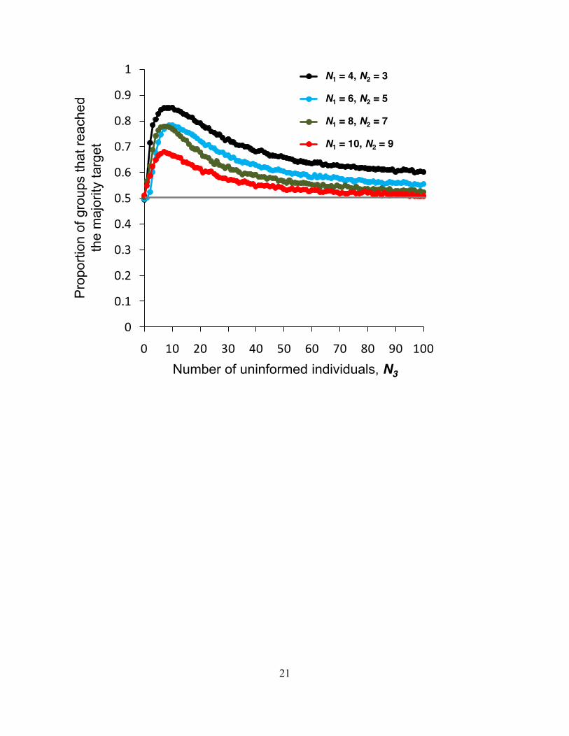
F ig. S2 The role of uninformed individuals for a range of N1 and N2 and an initial 2 at which there was a close-to-equal probability of selecting each target. See main text for discussion of this figure. All other parameters are as for Fig. 1b. 20,000 replicates per data point.

21

0

0.1

0.2

0.3

0.4

0.5

0.6

0.7

0.8

0.9

1

0 10 20 30 40 50 60 70 80 90 100

4  vs  3

6  vs  5

8  vs  7

10  vs  9

N1 = 4, N2 = 3

N1 = 6, N2 = 5

N1 = 8, N2 = 7

N1 = 10, N2 = 9

Number of uninformed individuals, N3

Prop

ortio

n of

gro

ups

that

reac

hed

the

maj

ority

targ

et

22

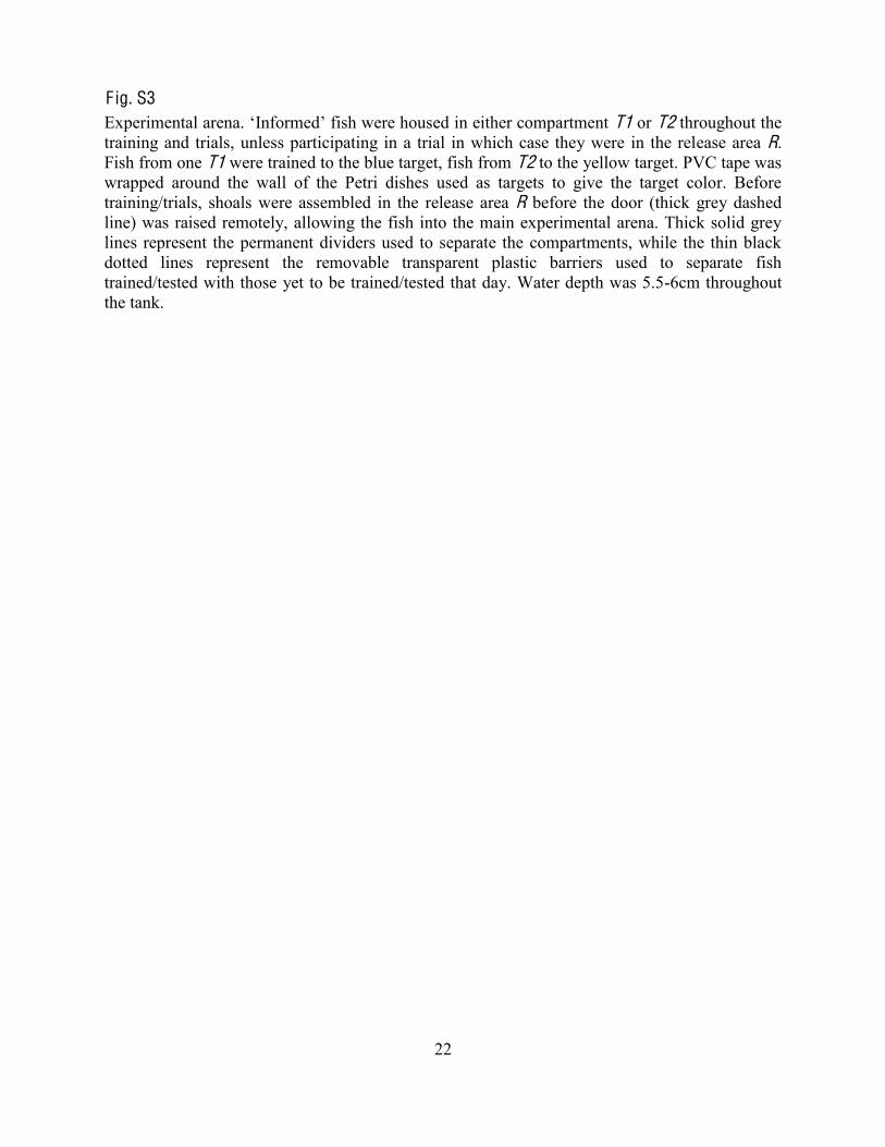
F ig. S3 T1 or T2 throughout the

training and trials, unless participating in a trial in which case they were in the release area R. Fish from one T1 were trained to the blue target, fish from T2 to the yellow target. PVC tape was wrapped around the wall of the Petri dishes used as targets to give the target color. Before training/trials, shoals were assembled in the release area R before the door (thick grey dashed line) was raised remotely, allowing the fish into the main experimental arena. Thick solid grey lines represent the permanent dividers used to separate the compartments, while the thin black dotted lines represent the removable transparent plastic barriers used to separate fish trained/tested with those yet to be trained/tested that day. Water depth was 5.5-6cm throughout the tank.

23

210cm

120cm

10cm

14cm

35cm

18cm

18cm

36.5cm

Blue target

Yellow targetT1

T2

R

24

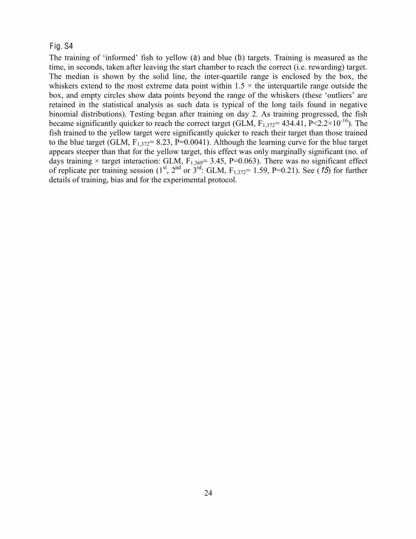
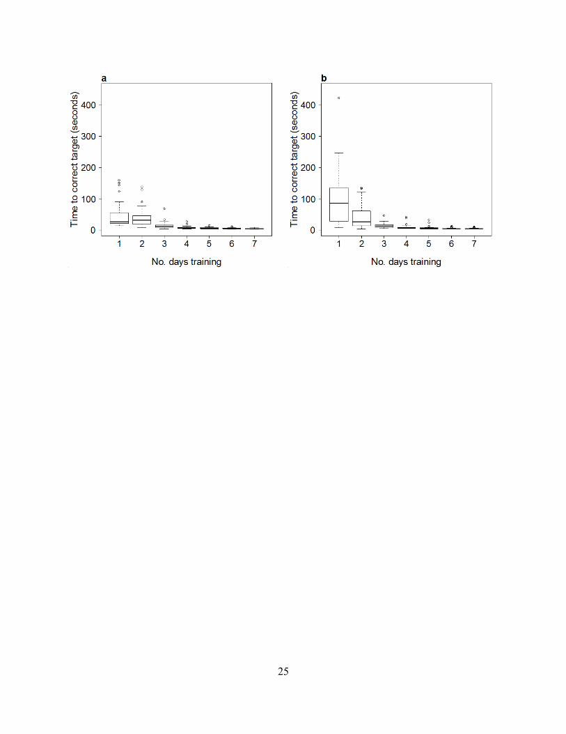
F ig. S4 to yellow (a) and blue (b) targets. Training is measured as the

time, in seconds, taken after leaving the start chamber to reach the correct (i.e. rewarding) target. The median is shown by the solid line, the inter-quartile range is enclosed by the box, the whiskers extend to the most extreme data point within 1.5 × the interquartile range outside the

retained in the statistical analysis as such data is typical of the long tails found in negative binomial distributions). Testing began after training on day 2. As training progressed, the fish became significantly quicker to reach the correct target (GLM, F1,372= 434.41, P<2.2×10-16). The fish trained to the yellow target were significantly quicker to reach their target than those trained to the blue target (GLM, F1,372= 8.23, P=0.0041). Although the learning curve for the blue target appears steeper than that for the yellow target, this effect was only marginally significant (no. of days training × target interaction: GLM, F1,369= 3.45, P=0.063). There was no significant effect of replicate per training session (1st, 2nd or 3rd: GLM, F1,372= 1.59, P=0.21). See (15) for further details of training, bias and for the experimental protocol.

25

 

26

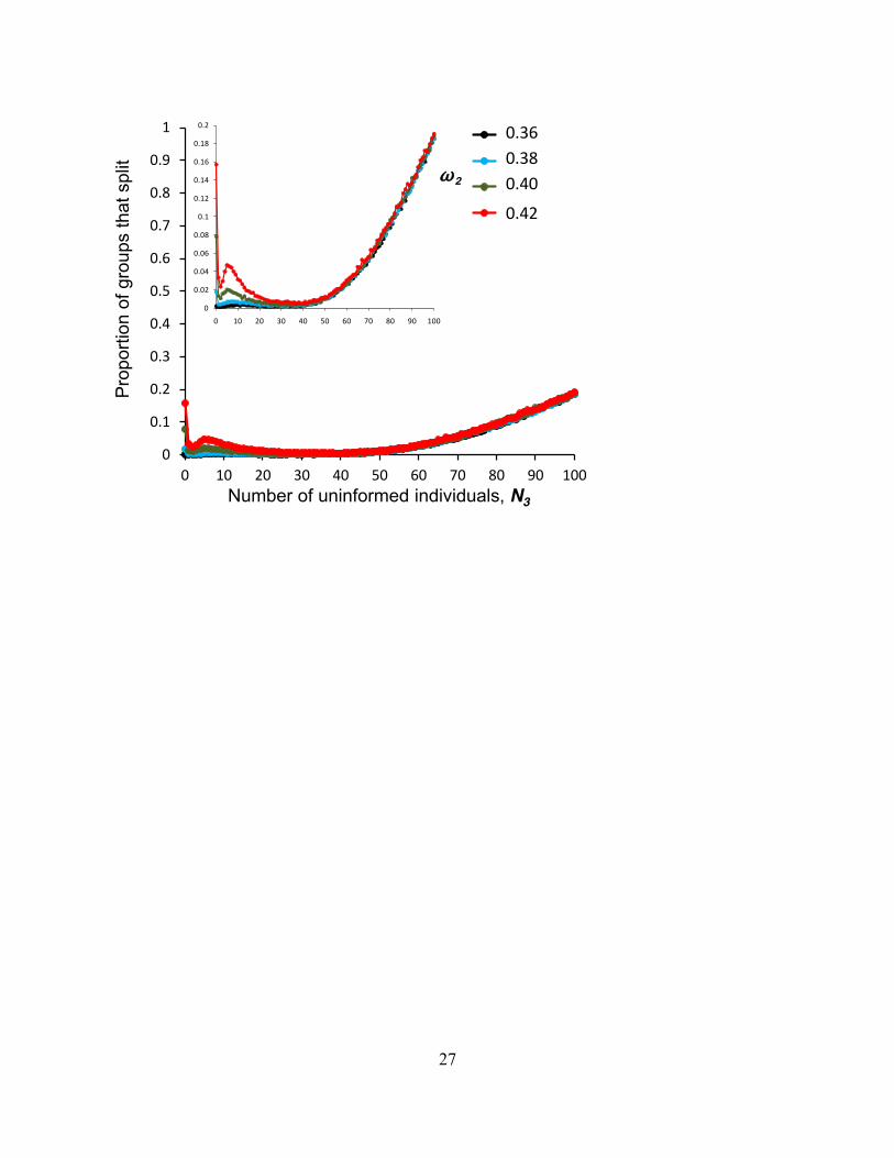
F ig. S5 The effect of uninformed individuals on group fragmentation (inset, the same data on a reduced Y-scale)

compared to the 0 uninformed case, at least until groups reach a substantial size and inevitable constraints related to locality of interactions consistently increases group fragmentation probability. However a lesser intermediate peak in group fragmentation also tends to occur in the regime where the uninformed individuals are present, but below their maximally influential numbers (c.f. Fig. 1b). Parameters are as for Fig. 1b.

27

0

0.02

0.04

0.06

0.08

0.1

0.12

0.14

0.16

0.18

0.2

0 10 20 30 40 50 60 70 80 90 100

Series1

Series2

Series3

Series4

0

0.1

0.2

0.3

0.4

0.5

0.6

0.7

0.8

0.9

1

0 10 20 30 40 50 60 70 80 90 100

0.36

0.38

0.4

0.42

0.36

0.38

0.40

0.42

Pro

porti

on o

f gro

ups

that

spl

it

Number of uninformed individuals, N3

2

28

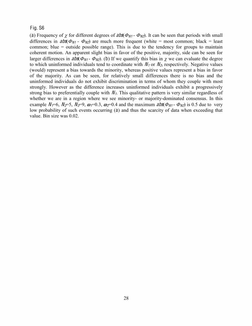
F ig. S6 (a) Frequency of for different degrees of abs( N1 - N2). It can be seen that periods with small differences in abs( N1 - N2) are much more frequent (white = most common; black = least common; blue = outside possible range). This is due to the tendency for groups to maintain coherent motion. An apparent slight bias in favor of the positive, majority, side can be seen for larger differences in abs( N1 - N2). (b) If we quantify this bias in we can evaluate the degree to which uninformed individuals tend to coordinate with N1 or N2, respectively. Negative values (would) represent a bias towards the minority, whereas positive values represent a bias in favor of the majority. As can be seen, for relatively small differences there is no bias and the uninformed individuals do not exhibit discrimination in terms of whom they couple with most strongly. However as the difference increases uninformed individuals exhibit a progressively strong bias to preferentially couple with N1. This qualitative pattern is very similar regardless of whether we are in a region where we see minority- or majority-dominated consensus. In this example N1=6, N2=5, N3=9, 1=0.3, 2=0.4 and the maximum abs( N1 - N2) is 0.5 due to very low probability of such events occurring (a) and thus the scarcity of data when exceeding that value. Bin size was 0.02.

29

0.0 0.1 0.2 0.3 0.4 0.5

0.1

0.2

0.3

0.4

0.5

0.0Diff

eren

ce b

etw

een

info

rmed

sub

sets

ab

s(N1

 -­‐N2)

Relative bias of

0.2 0.4 0.6 0.8 1.0-­‐1.0 -­‐0.8 -­‐0.6 -­‐0.4 -­‐0.2

0.1

0.2

0.3

0.4

0.5

0.0Diff

eren

ce b

etw

een

info

rmed

sub

sets

ab

s(N1

 -­‐N2)

a b

0.80.70.60.50.40.30.20.10.0

30

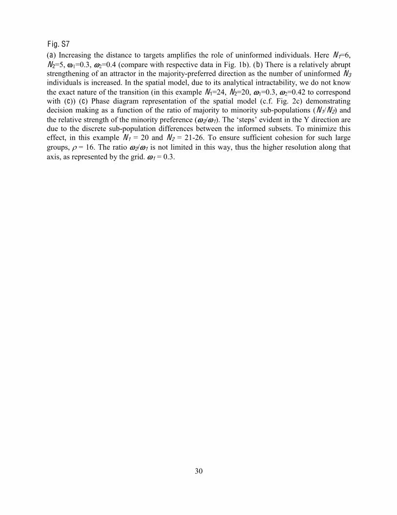
F ig. S7 (a) Increasing the distance to targets amplifies the role of uninformed individuals. Here N1=6, N2=5, 1=0.3, 2=0.4 (compare with respective data in Fig. 1b). (b) There is a relatively abrupt strengthening of an attractor in the majority-preferred direction as the number of uninformed N3 individuals is increased. In the spatial model, due to its analytical intractability, we do not know the exact nature of the transition (in this example N1=24, N2=20, 1=0.3, 2=0.42 to correspond with (c)) (c) Phase diagram representation of the spatial model (c.f. Fig. 2c) demonstrating decision making as a function of the ratio of majority to minority sub-populations (N1/N2) and the relative strength of the minority preference ( 2/ 1due to the discrete sub-population differences between the informed subsets. To minimize this effect, in this example N1 = 20 and N2 = 21-26. To ensure sufficient cohesion for such large groups, = 16. The ratio 2/ 1 is not limited in this way, thus the higher resolution along that axis, as represented by the grid. 1 = 0.3.

31

Prop

ortio

n of

gro

ups

that

re

ache

d th

e m

ajor

ity ta

rget

Deg

ree

of a

lignm

ent w

ith th

e m

ajor

ity-p

refe

rred

dire

ctio

nNumber of uninformed

individuals, N3

Number of uninformed individuals, N3

Num

eric

al a

dvan

tage

of t

he

maj

ority

(N1/N

2)

Relative strength of the minority preference 2/ 1

a b c

32

F ig. S8 Majority success rate for the convention model. The proportion of trials in which the majority preferred state is reached for increasing numbers of uninformed individuals is shown. Different lines represent system size scaling, with the proportion of individuals held constant. N1.=6x, N2 =5x where x is indicated by the legend. Red dashed line shows the approximate threshold obtained in the large N limit (see Equation 19 of 3.2 for details).

33

34

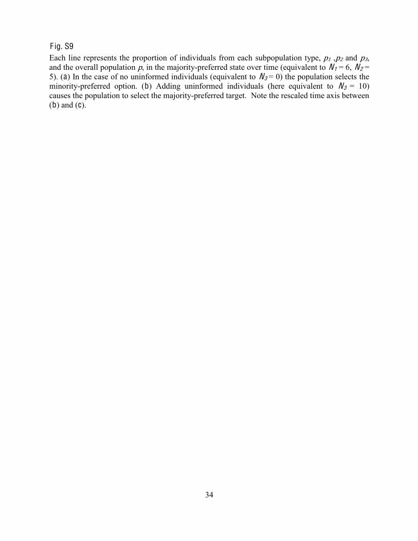
F ig. S9 Each line represents the proportion of individuals from each subpopulation type,  p1 ,p2 and p3, and the overall population p, in the majority-preferred state over time (equivalent to N1 = 6, N2 = 5). (a) In the case of no uninformed individuals (equivalent to N3 = 0) the population selects the minority-preferred option. (b) Adding uninformed individuals (here equivalent to N3 = 10) causes the population to select the majority-preferred target. Note the rescaled time axis between (b) and (c).

35

36

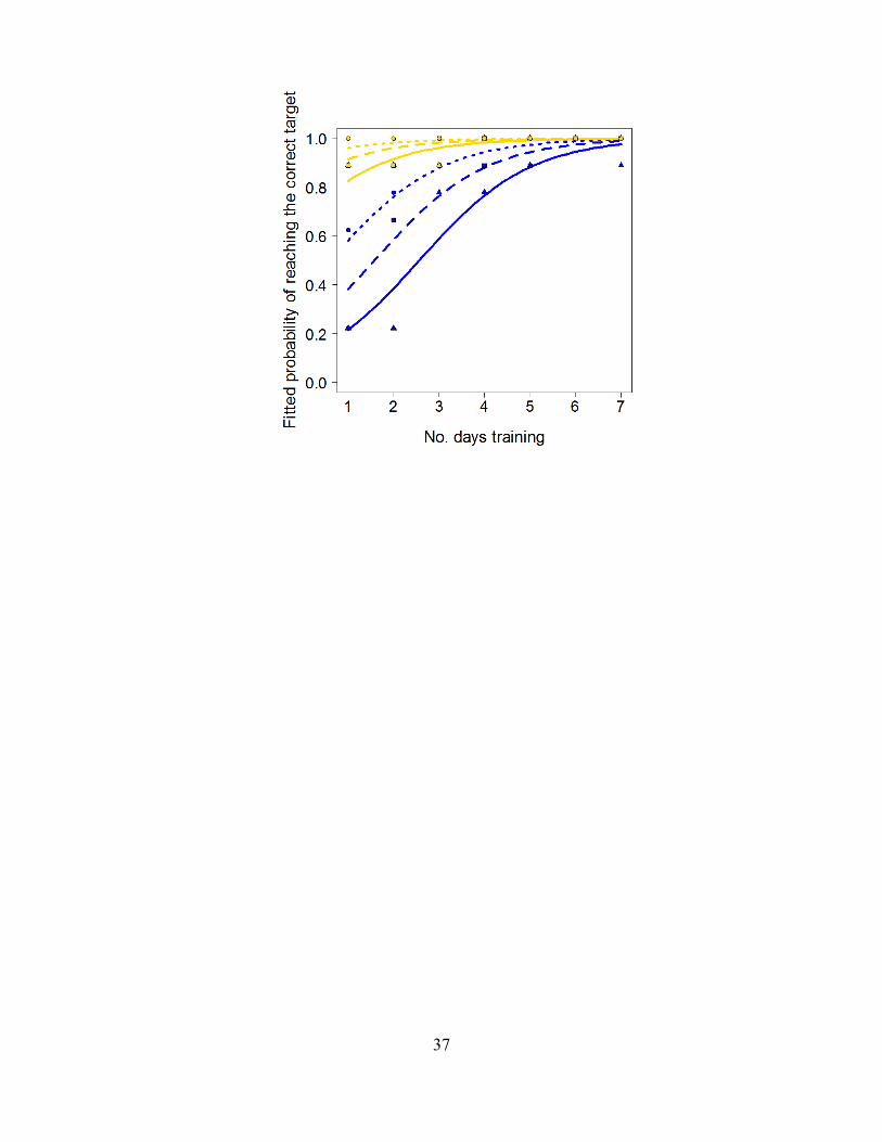
F ig. S10 Factors affecting whether the correct target, i.e. the target holding the food reward, was reached first during training. As expected with more days of training (x axis) the fish were more likely to reach the their preferred target first (GLM, F1,373= 75.13, P<2.2×10-16). Similarly, the fish were more likely to reach their preferred target, as opposed to the non-preferred target, as their three consecutive triplicate trainings progressed (solid line and triangles is the 1st training per session, dashed and squares is the 2nd, and dotted and circles is the 3rd; GLM, F1,373= 14.54, P=0.00016). The bias towards the yellow target was also significant, with fish trained to this target more likely to reach the correct target than fish trained to the blue target (GLM, F1,373= 57.23, P<3.06×10-13). There were no significant interaction terms (which were removed from the model); thus these 3 effects were independent of one another. The curves show fitted relationships from the main effects model, while points show the proportion of trainings where the correct target was reached first. Line color indicates color of the target.

37

38

F ig. S11 The effect of the 3 explanatory variables on whether the majority target was reached in the consensus trials. Fitted data is shown from the model in Table S1 after the 3 way interaction term was removed. Solid lines represent 0 naive trials, dashed lines 5 naive trials, and dotted lines 10 naive trials. Line color indicates color of the target, with the three lines starting in the top left corner of the figure being yellow. The bias for the yellow target was greatest when the fish were less well trained (i.e. when they took longer to reach the target during training); the probability of the majority winning was close to 100% when trained to the yellow target, but less than 50% when trained to the blue target. As the training and trials progressed (left to right along the x axis, with the fish reaching the target sooner in training), this bias decreased, yielding the significant Training × Target interaction in Table S1. This was not sensitive to the number of naive individuals in the shoal, indicated by the lack of a 3 way interaction between the two variables (Table S1). This result shows that the effect of naive individuals was not affected by the amount of training within the range tested.

39

40

F ig. S12 (a) Simulations of a group of 15 individuals that exhibit a consistent bias towards the minority-preferred target (bias strength = 3). Increasing 3 asymptotically increases preference of the minority-preferred target. (b) Investigating the respective role of intrinsic bias towards the minority-preferred target ( 3) to our results. Parameters as in Fig. S7a. N1 = 6, N2 = 5, w1 = 0.3, w2 = 0.4. Despite the bias, addition of N3 individuals still promotes the majority-opinion (compared to having no N3) but this effect weakens as bias to the minority-preferred target increases. Results shown from 1200 replicates per point.

41

0

0.1

0.2

0.3

0.4

0.5

0.6

0.7

0.8

0.9

1

0.002 0.004 0.006 0.008 0.01

0

0.1

0.2

0.3

0.4

0.5

0.6

0.7

0.8

0.9

1

0 1 2 3 4 5 6 7 8 9 10

0

0.002

0.004

0.006

0.008

0.01

3

Number of untrained, but biased, individuals, N3

Pro

porti

on o

f gro

ups

reac

hing

th

e m

ajor

ity ta

rget

Pro

porti

on o

f gro

ups

reac

hing

th

e m

ajor

ity ta

rget

3

a b

42

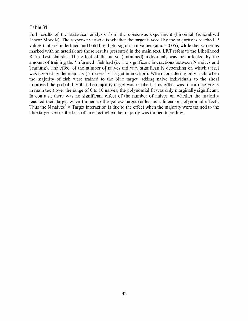
Table S1 Full results of the statistical analysis from the consensus experiment (binomial Generalised Linear Models). The response variable is whether the target favored by the majority is reached. P values that are underlined and bold marked with an asterisk are those results presented in the main text. LRT refers to the Likelihood Ratio Test statistic. The effect of the naive (untrained) individuals was not affected by the

Training). The effect of the number of naives did vary significantly depending on which target was favored by the majority (N naives2 × Target interaction). When considering only trials when the majority of fish were trained to the blue target, adding naive individuals to the shoal improved the probability that the majority target was reached. This effect was linear (see Fig. 3 in main text) over the range of 0 to 10 naives; the polynomial fit was only marginally significant. In contrast, there was no significant effect of the number of naives on whether the majority reached their target when trained to the yellow target (either as a linear or polynomial effect). Thus the N naives2 × Target interaction is due to the effect when the majority were trained to the blue target versus the lack of an effect when the majority was trained to yellow.    

43

Term Data Degrees of freedom L R T P value

N naives2 ×Training × Target All 2,96 1.69 0.43

N naives2 × Training All 2,98 0.96 0.62

N naives2 × Target All 2,98 6.47 0.039

Training × Target All 1,98 5.59 0.018

N naives2 Blue majority 2,51 5.65 0.059

N naives* Blue majority 1,52 5.60 0.018

N naives2 Yellow majority 2,51 4.28 0.12

N naives* Yellow majority 1,52 0.14 0.71

References and Notes 1. K. Arrow, Social Choices and Individual Values (Yale Univ. Press, New Haven, CT, ed. 2,

1963).

2. J. M. Buchanan, G. Tullock, The Calculus of Consent: Logical Foundations of Constitutional Democracy (Liberty Fund, Indianapolis, IN, 1958).

3. L. Conradt, T. J. Roper, Group decision-making in animals. Nature 421, 155 (2003). doi:10.1038/nature01294 Medline

4. L. Conradt, T. J. Roper, Consensus decision making in animals. Trends Ecol. Evol. 20, 449 (2005). doi:10.1016/j.tree.2005.05.008 Medline

5. I. D. Couzin, J. Krause, N. R. Franks, S. A. Levin, Effective leadership and decision-making in animal groups on the move. Nature 433, 513 (2005). doi:10.1038/nature03236 Medline

6. A. J. King, D. D. P. Johnson, M. Van Vugt, The origins and evolution of leadership. Curr. Biol. 19, R911 (2009). doi:10.1016/j.cub.2009.07.027 Medline

7. J. Krause, G. D. Ruxton, Living in Groups (Oxford Univ. Press, Oxford, 2002).

8. J. Mansbridge, Beyond Adversary Democracy (The Univ. of Chicago Press, Chicago, 1983).

9. M. Olson Jr., The Logic of Collective Action: Public Goods and the Theory of Groups (Harvard Univ. Press, Cambridge, MA, 1971).

10. W. Riker, Liberalism Against Populism: A Confrontation Between the Theory of Democracy and the Theory of Social Choice (W. H. Freeman, San Francisco, 1982).

11. T. D. Seeley, Honeybee Democracy (Princeton Univ. Press, Princeton, NJ, 2010).

12. A. J. Ward, J. E. Herbert-Read, D. J. T. Sumpter, J. Krause, Fast and accurate decisions through collective vigilance in fish shoals. Proc. Natl. Acad. Sci. U.S.A. 108, 2312 (2011). doi:10.1073/pnas.1007102108 Medline

13. L. Conradt, J. Krause, I. D. Couzin, T. J. Roper, “Leading according to need” in self-organizing groups. Am. Nat. 173, 304 (2009). doi:10.1086/596532 Medline

14. S. Issacharoff, Democracy and collective decision making. Int. J. Const. Law 6, 231 (2008). doi:10.1093/icon/mon003

15. Materials and methods are available as supporting material on Science Online.

16. Y. Katz, K. Tunstrøm, C. C. Ioannou, C. Huepe, I. D. Couzin, Inferring the structure and dynamics of interactions in schooling fish. Proc. Natl. Acad. Sci. U.S.A. 108, 18720 (2011).

17. C. Huepe, G. Zschaler, A.-L. Do, T. Gross, Adaptive-network models of swarm dynamics. New J. Phys. 13, 073022 (2011). doi:10.1088/1367-2630/13/7/073022

18. H. P. Young, Individual Strategy and Social Structure: An Evolutionary Theory of Institutions (Princeton Univ. Press, Princeton, NJ, 1998).

19. S. G. Reebs, Can a minority of informed leaders determine the foraging movements of a fish shoal? Anim. Behav. 59, 403 (2000). doi:10.1006/anbe.1999.1314 Medline

20. R. Spence, R. Smith, Innate and learned colour preference in the zebrafish, Danio rerio. Ethology 114, 582 (2008). doi:10.1111/j.1439-0310.2008.01515.x

21. P. Holme, M. E. J. Newman, Phys. Rev. E 74, 056108 (2006).

22. F. Vazquez, V. M. Eguíluz, M. San Miguel, Generic absorbing transition in coevolution dynamics. Phys. Rev. Lett. 100, 108702 (2008). doi:10.1103/PhysRevLett.100.108702 Medline

23. D. H. Zanette, S. Gil, Opinion spreading and agent segregation on evolving networks. Physica D 224, 156 (2006). doi:10.1016/j.physd.2006.09.010

24. B. Nabet, N. E. Leonard, I. D. Couzin, S. A. Levin, Dynamics of decision making in animal group motion. J. Nonlinear Sci. 19, 399 (2009). doi:10.1007/s00332-008-9038-6

25. R. A. Holley, T. M. Liggett, Ergodic theorems for weakly interacting infinite systems and the voter model. Ann. Probab. 3, 643 (1975). doi:10.1214/aop/1176996306

26. R. Durrett, S. A. Levin, The importance of being discrete (and spatial). Theor. Popul. Biol. 46, 363 (1994). doi:10.1006/tpbi.1994.1032

27. H. P. Young, The evolution of conventions. Econometrica 61, 57 (1993). doi:10.2307/2951778