SUBSEA PIPE LAYING IN COASTAL AREA - hrbi.hr · SUBSEA PIPE LAYING IN COASTAL AREA ... morskog dna...

Većeslav ČORIĆ, Ivan ĆATIPOVIĆ, Jadrank, RADANOVIĆ Faculty of Mechanical Engineering and Naval Architecture, Ivana Lučuća 5, 10000 Zagreb

SUBSEA PIPE LAYING IN COASTAL AREA

Summary

Two essential problems characterize design and installation of the subsea pipeline in the coastal area: strong hydrodynamic loading due to waves and sea current as well as the bending loading of the pipe on the curved sea bottom. In the article it is given the description of structural and stability analysis of the concrete coated steel pipe when it is laid on the uneven sea bottom near the coast. The equilibrium shape of the bended pipeline when it is exposed to gravitational, operating and hydrodynamic loading is analyzed by the nonlinear finite element model which includes the large displacement and the contact problems between the pipe and sea bottom. The illustrative example shows how to define the relevant design sea state necessary for assessment of the subsea pipeline structural integrity and stability on the sea bottom. The results obtained by time simulations are compared with the accepted standards.

Key words: subsea pipeline, hydrodynamic loading, bending of the elastic body on the curved support

POLAGANJE PODMORSKIH CJEVOVODA U OBALNOM PODRU ČJU

Sažetak

Hidrodinamičko opterećenje valova i morske struje te savijanje uslijed zakrivljenosti morskog dna dva su bitna problema kojima u projektu podmorskih cjevovoda za transport nafte i plina treba posvetiti nužnu pažnju u obalnom području. U članku je opisan metodološki postupak dimenzioniranja i provjere stabilnosti čeličnog, betonom obloženog podmorskog cjevovoda, slobodno položenog na zakrivljeno morsko dno. Ravnotežni položaj savinutog cjevovoda koji je izložen radnom, gravitacijskom i hidrodinamičkom opterećenju, odreñen je na nelinearnom strukturnom modelu konačnih elemenata. Model uključuje geometrijsku nelinearnost uslijed velikih pomaka i nelinearnost uslijed kontaktnog problem izmeñu cjevovoda i morskog dna. Ilustrativnim primjerom prikazan je način definiranja projektnog stanja mora i dana je usporedba bitnih rezultata dobivenih vremenskom simulacijom s rezultatima važećih propisa.

Ključne riječi: podmorski cjevovod, hidrodinamičko opterećenje, savijanje elastičnog tijela na neravnoj podlozi

XX Symposium SORTA2012 Subsea Pipe Laying in Coastal Area

1. Introduction

Two fundamental problems are present during laying a subsea gas/oil pipeline on the sea bottom when it approaches to the coast:

- sea becomes shallow and the pipeline is exposed to strong sea waves and current actions resulting in significant lateral hydrodynamic loading,

- the pipe is bended on uneven and curved sea bottom and additional stress occurs; besides inner hydrodynamic loading appears in bended pipeline (due to pressure and fluid flow in curved pipe).

In coastal areas appropriate pipeline protection from hydrodynamic loading is required to insure its bottom stability. The steel subsea pipe is regularly coated by heavy concrete to increase gravity load which compensates the effect of hydrostatic buoyancy. The effective pipeline weight and bottom friction must be sufficient to resist all lateral hydrodynamic loads. In the opposite case the pipeline must be additionally protected from lateral loading. The resulting equivalent stress which consists of hoop, longitudinal and bending stress, must be controlled by the allowable trace curvature. Finally, if the pipe free spans are too large, what may happen on uneven and curved sea bottom, vortex induced vibration (VIV) occurs. Such situations sometimes require expensive subsea intervention in construction works on the sea bottom. The shallow sea and usually limited maneuvering area unable application of specialized pipe-lying barge or similar type of supporting vessels. In these circumstances the pipeline installation becomes extremely expensive and minimization of the subsea intervention work must be performed: the minimization of the pipeline route correction becomes a part of the analysis.

1. Pipeline route

The most important step in the subsea pipeline engineering is the choice of the pipeline route. It is preceded by the extensive sea bottom survey which includes bathymetry and soil mechanic properties measurements. Sometimes the choice of the route is decided by the least unfavorable route from all applicable.

100 200 300 400 500 600 700

60

50

40

30

20

10

0

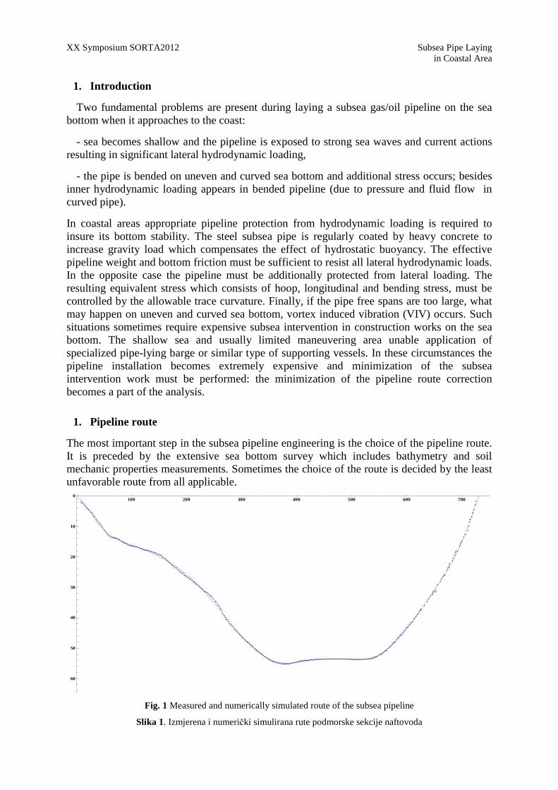
Fig. 1 Measured and numerically simulated route of the subsea pipeline

Slika 1. Izmjerena i numerički simulirana rute podmorske sekcije naftovoda

Subsea Pipe Laying XX Symposium SORTA2012 in Coastal Area

The bathymetry record of such typical subsea pipeline route it is presented in Fig. 1. The analysis of the problem begins with appropriate numerical modeling of the route, i.e. defining the suitable function z(x) which presents the measured sea bottom bathymetry with sufficient accuracy:

( ) ( ) ( )xPxdxz n≈= (1)

In the above relation d(x) is measured sea depth on section x and Pn(x) is numerical approximation, usually given by the polynomial of nth degree. The comparison between the measured bathymetry and approximation by polynomial of 17th degree is shown in Fig. 1.

The radius R(x) of the sea bottom curvature then follows strait forward from (1):

( )( )xP

dx

d

dx

zd

dx

dz

xR

n2

2

2

2

2/32

11

≈

+

= (2)

On the other side, when the pipe is in static equilibrium position on the sea bottom, the pipe flexure line w(x) gives the following relation for the bending radius r(x) after the second order values are neglected:

( ) ( ) ( )EI

xMxw

dx

d

xr−=≈

2

21 (3)

M(x) and EI are bending moment and bending stiffness of the composite pipe section. The comparison of two curvature radii, i.e. R(x) and r(x) gives the first necessary condition for the safe pipe laying in the chosen subsea route: the sea bottom curvature radius R(x) should be larger than pipe bending radius r(x) ≥ relast, where relast is given by the following approximate relation:

yF

ay

aF

allow

aelast

E

D

aDS

W

EIS

M

EIr

σσ

+≈== 212

1 (4)

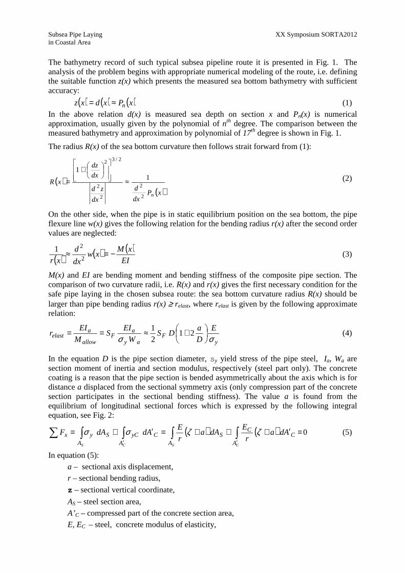
In the equation D is the pipe section diameter, sy yield stress of the pipe steel, Ia, Wa are section moment of inertia and section modulus, respectively (steel part only). The concrete coating is a reason that the pipe section is bended asymmetrically about the axis which is for distance a displaced from the sectional symmetry axis (only compression part of the concrete section participates in the sectional bending stiffness). The value a is found from the equilibrium of longitudinal sectional forces which is expressed by the following integral equation, see Fig. 2:

( ) ( ) 0=′+++=′+= ∫∫∫∫∑′′ CSCS A

CC

AS

ACyC

ASyx Ada

r

EdAa

r

EAddAF ζζσσ (5)

In equation (5):

a – sectional axis displacement,

r – sectional bending radius,

z – sectional vertical coordinate,

AS – steel section area,

A’C – compressed part of the concrete section area,

E, EC – steel, concrete modulus of elasticity,


R_ coR _ci R_s

a

t_co

t_ci t _s

vanjski omotaccelicna cijev

unutarnji omotac

es

ec

s s

s c

Fig. 2 The composite subsea pipeline section (section asymmetric bending)

Slika 2.Kompozitni presjek podmorskog cjevovoda (nesimetrično savijanje presjeka)

The safety factor SF in (4) depends on the material coefficient gm and coefficient of pipe efficiency hR

R

mFS

ηγ= (6)

The material coefficient gm depends on the pipeline class, location and steel type of the subsea pipeline and it is usually strictly defined by the chosen standard for such type of a structure, [2]. The efficiency coefficient hR is unknown and must be assumed at the beginning of a design procedure on the basis of the designer judgment: it defines a ratio between a part of the pipe operating stress level sP(Dp) and part due to pipe bending sB(M). In the present example it is assumed:

60,0=Rη It is assumed that 40% of the pipe structural capacity is absorbed by the working (pressure) and environmental loading (waves, sea current) and rest 60% is spent into elastic bending stress. The coated steel pipe has relatively high bending stiffness and the laid subsea pipeline will not be continuously supported on the sea bottom. The free spans of different lengths result with additional pipe bending and further reduction of bending radius r(x). The assumed coefficient of efficiency hR must be verified after the detailed FEM analysis is performed.

2. Pipeline on the sea bottom

The subsea pipelines are usually freely laid from the sea surface. The laid pipeline takes static equilibrium position under the action of gravity, hydrostatic, and frictional forces on the sea bottom. In the first step of the analysis it is assumed that only gravity and hydrostatic forces act onto the pipe. The pipe is slowly falling down in vertical plane and the problem may be idealized as a low speed collision (inertial forces are neglected) between the elastic pipe body and partly rigid/elastic sea bottom. If the risks from earthquake exist in the area, the liquefaction phenomena must be expected and the sea bottom may lose its bearing capacity. Such critical parts are modeled as an elastic body with appropriate stiffness which depends on the geo-mechanical characteristics and bearing capacity.

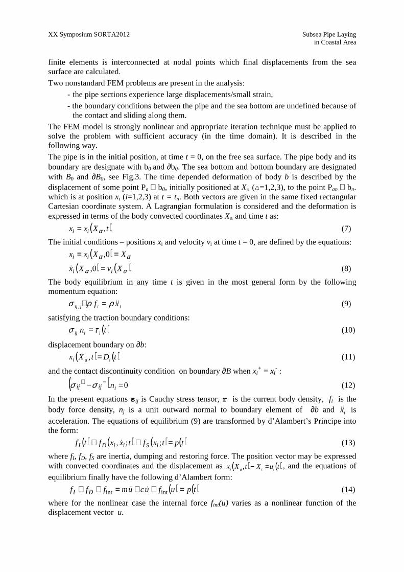
The equilibrium position of the pipeline is calculated by the dynamic FEM model consists of the beam finite elements, representing the pipe structure, and shell finite elements modeling the sea bottom. The shell elements nodes are fixed in rigid part of the bottom and supported by adequate spring elements in the part where liquefaction is expected, see Fig.4. The mesh of


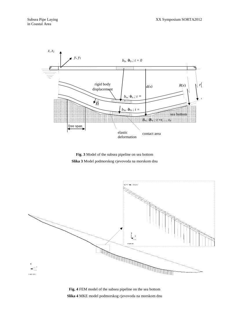
Fig. 3 Model of the subsea pipeline on sea bottom

Slika 3 Model podmorskog cjevovoda na morskom dnu

Fig. 4 FEM model of the subsea pipeline on the sea bottom

Slika 4 MKE model podmorskog cjevovoda na morskom dnu

rigid body displacement

elastic deformation

sea bottom

y, y1

z, z1

free span

d(x)

contact area

b0,�b0 ; t = 0

bn,�bn ; t = tn

bN,�bN ; t =

R(x) (r x w x

BN,�BN ; t =t,…, tN

w(x)

nr

rigid body displacement


finite elements is interconnected at nodal points which final displacements from the sea surface are calculated.

Two nonstandard FEM problems are present in the analysis:

- the pipe sections experience large displacements/small strain,

- the boundary conditions between the pipe and the sea bottom are undefined because of the contact and sliding along them.

The FEM model is strongly nonlinear and appropriate iteration technique must be applied to solve the problem with sufficient accuracy (in the time domain). It is described in the following way.

The pipe is in the initial position, at time t = 0, on the free sea surface. The pipe body and its boundary are designate with b0 and ∂b0. The sea bottom and bottom boundary are designated with B0 and ∂B0, see Fig.3. The time depended deformation of body b is described by the displacement of some point Pa ∈ b0, initially positioned at Xa (a=1,2,3), to the point Pan ∈ bn. which is at position xi (i=1,2,3) at t = tn. Both vectors are given in the same fixed rectangular Cartesian coordinate system. A Lagrangian formulation is considered and the deformation is expressed in terms of the body convected coordinates Xa and time t as:

( )tXxx ii ,α= (7)

The initial conditions – positions xi and velocity vi at time t = 0, are defined by the equations:

( ) αα XXxx ii == 0,

( ) ( )αα XvXx ii =0,& (8)

The body equilibrium in any time t is given in the most general form by the following momentum equation:

iijij xf &&ρρσ =+, (9)

satisfying the traction boundary conditions:

( )tn iiij τσ = (10)

displacement boundary on ∂b:

( ) ( )tDtXx iai =, (11)

and the contact discontinuity condition on boundary ∂B when xi+ = xi

- :

( ) 0=− −+iijij nσσ (12)

In the present equations sij is Cauchy stress tensor, r is the current body density, fi is the body force density, nj is a unit outward normal to boundary element of ∂b and ix&& is

acceleration. The equations of equilibrium (9) are transformed by d’Alambert’s Principe into the form:

( ) ( ) ( ) ( )tptxftxxftf iSiiDI =++ ;;, & (13)

where fI, fD, fS are inertia, dumping and restoring force. The position vector may be expressed with convected coordinates and the displacement as ( ) ( )tuXtXx iiai =−, , and the equations of

equilibrium finally have the following d’Alambert form:

( ) ( )tpufucumfff DI =++=++ intint &&& (14)

where for the nonlinear case the internal force fint(u) varies as a nonlinear function of the displacement vector u.


For nonlinear problems the equations of motions are integrated by explicate central difference scheme.

2.1. Large displacement

The special beam element must be applied in the model because of large displacement/small strain problem. Appropriate type of the finite element is Belytschko beam element formulated in co-rotational technique, [5], [6]. The formulation separates the deformation displacements from the rigid body displacements which do not affects strains and associated strain energy. It is based on the following three ingredients:

- the relations between global and local variables,

- the angle of rotation of a co-rotating frame,

- the variationally consistent tangent stiffness matrix

The elongation of the beam is calculated directly from the original nodal coordinates (XJ,YJ,ZJ) and the total displacement (uxJ, uyJ, uzJ) while the bending moment are related to the deformation rotations through the standard beam element stiffness matrix. The beam element is allowed to have arbitrarily large displacements and rotations at the global level (so long as local beam element strains are small the results are valid). All beam elements are assumed to remain linear elastic.

2.2. Contact problem

Two bodies, the pipeline and the sea bottom, occupy regions b0 and B0 and boundaries ∂b0

and ∂B0 and have no common points in their initial configuration at time t = 0:

=00 Bb I ∅ (15)

At some later time tn > 0, the bodies occupy regions defined by forms bn, Bn and boundaries ∂bn , ∂Bn. As the deformed configurations cannot penetrate:

( ) =∂ nnn Bbb I\ ∅ (16)

as long as

=nn Bb I ∅, (17)

the equation of motion (13) remain uncoupled. In the time t when it is

≠nn Bb I ∅ (18)

the equations of motions are coupled in common points with limitation which follows from the elastic characteristics of the model.

Three distinct methods for handling the contact problem exist. They are referred as the kinematic constrain method, the penalty method and the distributed parameter method. The slave/master technique may be used to define the interfaces between bodies bn, Bn. It is defined in the coordinate system by listing in arbitrary order all beam nodes and triangular and quadrilateral segments (shell elements) that comprise master side of interface. The beam element nodes are referred as slave and the shell element nodes as master nodes. The slave search finds for each slave node its nearest point on the master surface. Lines drawn from a slave node to its nearest point will be perpendicular to the master surface.

In the kinematic constraint method constraints are imposed on the global equations of motion by transformation of the nodal displacement components of the slave nodes along the contact


interface. This transformation has the effect of eliminating the normal degree of freedom nodes. Impact and realize conditions are imposed to insure momentum conservation.

Several general purpose FEM software for multiphysics simulation are capable of dealing with already described problem, [6], [7], [8]. Results of the analysis by means of software from [6] are summarized in bending moment M(x) and shear force Q(x) diagrams, Fig. 5. Comparison of the equivalent stress svonMises level with allowable according to offshore standard [2] shows exceeding the limit value on critical parts of the pipeline, see Fig. 2.a), and some remedy measures have to be undertaken.

2.3. Optimisation of the subsea pipeline route correction

The purpose of seabed intervention is to ensure that the pipeline maintains structural integrity in all phases throughout its design life. There are several types of seabed intervention: rock dumping, trenching, burying and pre-sweping. The undersea work is extremely expensive and some optimisation of the route correction must be performed to minimise the additional expenses.

Sea bottom boundary ∂B0 is considered as a data set consisted of n points ( )( ) nixdx ii K,1,, = , defined by its approximation Pn(x), equation (1). The objective is finding

the best fit for data set that satisfies curvature condition stated with respect to relast in (4), i.e. to find the infimum1 of quadratic spline residuals:

( ) ( )

≥−∑

=elast

n

iii rxrfsplinequadraticisfxdxf )(,;inf

1

(19)

where )(xrf is curvature radius. The solution of this problem is easy to find, but the curvature radius of the resulting function has discontinuity of first kind what introduces the concentrate reactions supporting the pipe on the sea bottom. That problem is solved simply by convolution of obtained solution and smooth function αρ which has the following form:

( )

≥

<=−

1,0

1,1

12

x

xexx

ρ (20)

( )

=α

ρα

ραxc

x (21)

In the above equations ( )1−∞

∞−

= ∫ dyyc ρ , and α is small positive number.

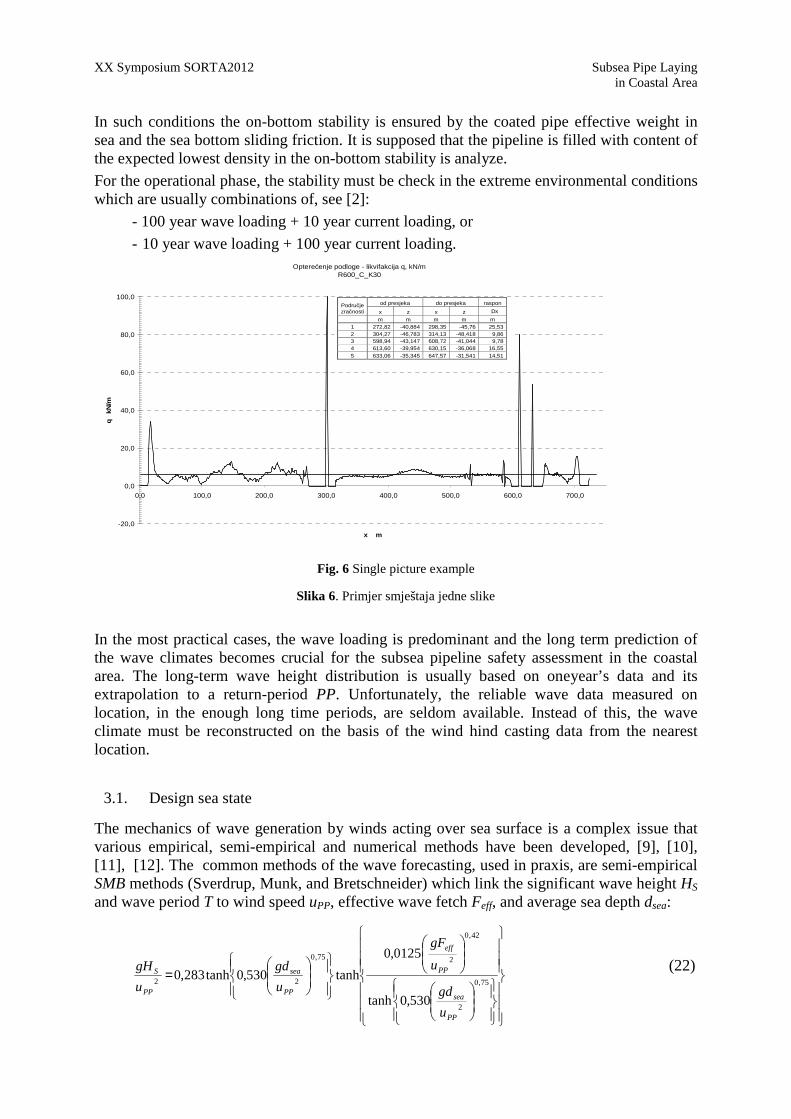
Bending moment M(x) and shear force Q(x) diagrams of the subsea pipeline after intervention and the trace correction are shown in Fig. 5.b). The distribution of supporting reaction force q(x), which is important for the pipeline on-bottom stability, is shown in Fig. 6 for the final geometry of the corrected route.

1 Infimum – the largest lower bound


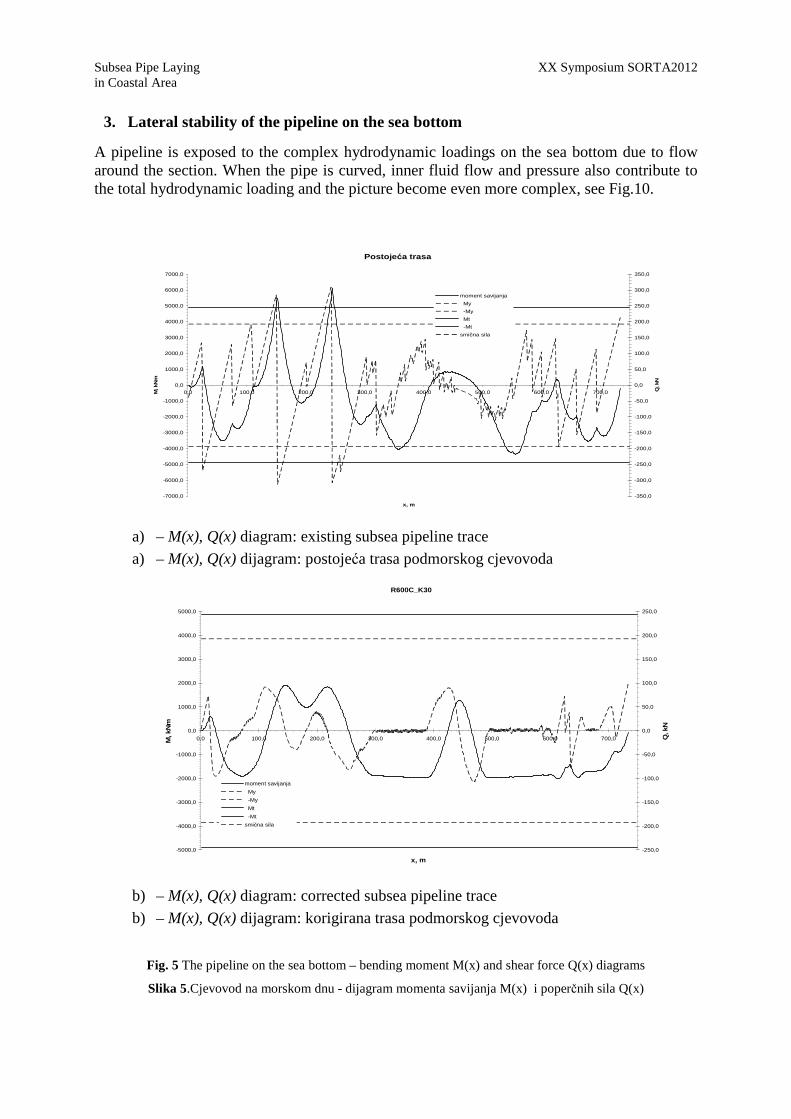
3. Lateral stability of the pipeline on the sea bottom

A pipeline is exposed to the complex hydrodynamic loadings on the sea bottom due to flow around the section. When the pipe is curved, inner fluid flow and pressure also contribute to the total hydrodynamic loading and the picture become even more complex, see Fig.10.

Postojeća trasa

-7000,0

-6000,0

-5000,0

-4000,0

-3000,0

-2000,0

-1000,0

0,0

1000,0

2000,0

3000,0

4000,0

5000,0

6000,0

7000,0

0,0 100,0 200,0 300,0 400,0 500,0 600,0 700,0

x, m

M, k

Nm

-350,0

-300,0

-250,0

-200,0

-150,0

-100,0

-50,0

0,0

50,0

100,0

150,0

200,0

250,0

300,0

350,0

Q, k

N

moment savijanja

My

-My

Mt

-Mt

smična sila

a) – M(x), Q(x) diagram: existing subsea pipeline trace

a) – M(x), Q(x) dijagram: postojeća trasa podmorskog cjevovoda

R600C_K30

-5000,0

-4000,0

-3000,0

-2000,0

-1000,0

0,0

1000,0

2000,0

3000,0

4000,0

5000,0

0,0 100,0 200,0 300,0 400,0 500,0 600,0 700,0

x, m

M, k

Nm

-250,0

-200,0

-150,0

-100,0

-50,0

0,0

50,0

100,0

150,0

200,0

250,0

Q, k

N

moment savijanja

My

-My

Mt

-Mt

smična sila

b) – M(x), Q(x) diagram: corrected subsea pipeline trace

b) – M(x), Q(x) dijagram: korigirana trasa podmorskog cjevovoda

Fig. 5 The pipeline on the sea bottom – bending moment M(x) and shear force Q(x) diagrams

Slika 5.Cjevovod na morskom dnu - dijagram momenta savijanja M(x) i poperčnih sila Q(x)


In such conditions the on-bottom stability is ensured by the coated pipe effective weight in sea and the sea bottom sliding friction. It is supposed that the pipeline is filled with content of the expected lowest density in the on-bottom stability is analyze.

For the operational phase, the stability must be check in the extreme environmental conditions which are usually combinations of, see [2]:

- 100 year wave loading + 10 year current loading, or

- 10 year wave loading + 100 year current loading. Opterećenje podloge - likvifakcija q, kN/m

R600_C_K30

-20,0

0,0

20,0

40,0

60,0

80,0

100,0

0,0 100,0 200,0 300,0 400,0 500,0 600,0 700,0

x m

q

kN/m

od presjeka do presjeka raspon Područje zračnosti x z x z Dx

m m m m m 1 272,82 -40,884 298,35 -45,76 25,53 2 304,27 -46,783 314,13 -48,418 9,86 3 598,94 -43,147 608,72 -41,044 9,78 4 613,60 -39,954 630,15 -36,068 16,55 5 633,06 -35,345 647,57 -31,541 14,51

Fig. 6 Single picture example

Slika 6. Primjer smještaja jedne slike

In the most practical cases, the wave loading is predominant and the long term prediction of the wave climates becomes crucial for the subsea pipeline safety assessment in the coastal area. The long-term wave height distribution is usually based on oneyear’s data and its extrapolation to a return-period PP. Unfortunately, the reliable wave data measured on location, in the enough long time periods, are seldom available. Instead of this, the wave climate must be reconstructed on the basis of the wind hind casting data from the nearest location.

3.1. Design sea state

The mechanics of wave generation by winds acting over sea surface is a complex issue that various empirical, semi-empirical and numerical methods have been developed, [9], [10], [11], [12]. The common methods of the wave forecasting, used in praxis, are semi-empirical SMB methods (Sverdrup, Munk, and Bretschneider) which link the significant wave height HS

and wave period T to wind speed uPP, effective wave fetch Feff, and average sea depth dsea:

=

75,0

2

42,0

275,0

22

530,0tanh

0125,0

tanh530,0tanh283,0

PP

sea

PP

eff

PP

sea

PP

S

u

gd

u

gF

u

gd

u

gH (22)


=

375,0

2

25,0

2375,0

2

833,0tanh

0770,0

tanh833,0tanh540,7

PP

sea

PP

eff

PP

sea

PP

u

gd

u

gF

u

gd

u

gT (23)

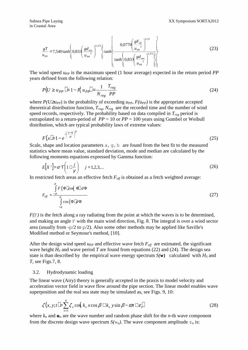
The wind speed uPP is the maximum speed (1 hour average) expected in the return period PP years defined from the following relation:

( ) ( )PP

T

NuFuUP

reg

regPPPP

11 =−=≥ (24)

where P(U≥uPP) is the probability of exceeding uPP, F(uPP) is the appropriate accepted theoretical distribution function, Treg, Nreg are the recorded time and the number of wind speed records, respectively. The probability based on data compiled in Treg period is extrapolated to a return-period of PP = 10 or PP = 100 years using Gumbel or Weibull distribution, which are typical probability laws of extreme values:

( )γ

αη

−−−=

u

exF 1 (25) Scale, shape and location parameters a,g,h are found from the best fit to the measured statistics where mean value, standard deviation, mode and median are calculated by the following moments equations expressed by Gamma function:

[ ] ,...3,2,11 =

+Γ= jj

XE jj

γα (26)

In restricted fetch areas an effective fetch Feff is obtained as a fetch weighted average:

( ) ( )

( )

cos

coseff

F d

F

d

α

αα

α

−

−

Φ Φ Φ=

Φ Φ

∫

∫

(27)

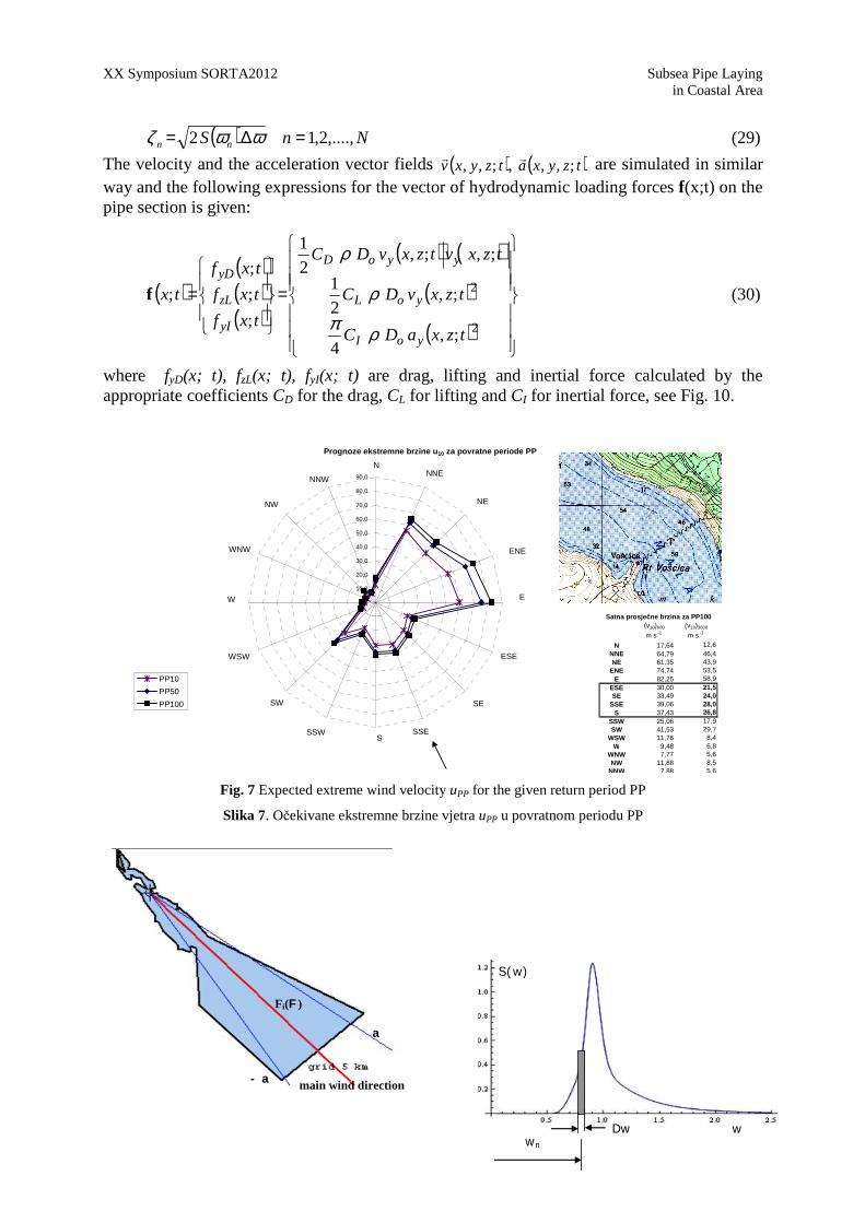
F(F) is the fetch along a ray radiating from the point at which the waves is to be determined, and making an angle F with the main wind direction, Fig. 8. The integral is over a wind sector area (usually from -p/2 to p/2). Also some other methods may be applied like Saville's Modified method or Seymour's method, [10].

After the design wind speed uPP and effective wave fetch Feff are estimated, the significant wave height HS and wave period T are found from equations (22) and (24). The design sea state is than described by the empirical wave energy spectrum S(w) calculated with HS and T, see Figs.7, 8.

3.2. Hydrodynamic loading

The linear wave (Airy) theory is generally accepted in the praxis to model velocity and acceleration vector field in wave flow around the pipe section. The linear model enables wave superposition and the real sea state may be simulated as, see Figs. 9, 10:

( ) ( )nnn

N

nn tykxktyx εωββζζ +−+=∑

=

sincoscos;,1

(28)

where kn and en are the wave number and random phase shift for the n-th wave component from the discrete design wave spectrum S(wn). The wave component amplitude zn is:


( ) NnS nn ,....,2,12 =∆= ωωζ (29)

The velocity and the acceleration vector fields ( ) ( )tzyxatzyxv ;,,,;,,rr are simulated in similar

way and the following expressions for the vector of hydrodynamic loading forces f(x;t) on the pipe section is given:

( )( )( )( )

( ) ( )

( )

( )

=

=

2

2

;,4

;,21

;,;,21

;

;

;

;

tzxaDC

tzxvDC

tzxvtzxvDC

txf

txf

txf

tx

yoI

yoL

yyoD

yI

zL

yD

ρπρ

ρ

f (30)

where fyD(x; t), fzL(x; t), fyI(x; t) are drag, lifting and inertial force calculated by the appropriate coefficients CD for the drag, CL for lifting and CI for inertial force, see Fig. 10.

Prognoze ekstremne brzine u10 za povratne periode PP

SE

SSES

SSW

SW

WSW

W

WNW

NW

NNWNNE

NE

ENE

E

ESE

N

0,0

10,0

20,0

30,0

40,0

50,0

60,0

70,0

80,0

90,0

PP10

PP50

PP100

(v10)600 (v10)3600

m s -1 m s -1

N 17,64 12,6NNE 64,79 46,4NE 61,35 43,9

ENE 74,74 53,5E 82,25 58,9

ESE 30,00 21,5SE 33,49 24,0

SSE 39,06 28,0S 37,43 26,8

SSW 25,06 17,9SW 41,53 29,7

WSW 11,76 8,4W 9,48 6,8

WNW 7,77 5,6NW 11,88 8,5

NNW 7,88 5,6

Satna prosječne brzina za PP100

Fig. 7 Expected extreme wind velocity uPP for the given return period PP

Slika 7. Očekivane ekstremne brzine vjetra uPP u povratnom periodu PP

Dw wn

w

S( w)

main wind direction - a

a

Fi(F )


Fig. 8 Effective wave fetch Fig. 9 Tabain sea spectrum of Adriatic sea

Slika 8. Efektivno valno privjetrište Slika 9. Tabainov spektar Jadranskog mora

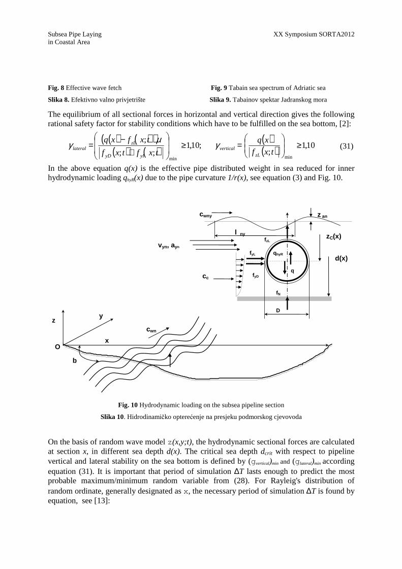
The equilibrium of all sectional forces in horizontal and vertical direction gives the following rational safety factor for stability conditions which have to be fulfilled on the sea bottom, [2]:

( ) ( )( )( ) ( )

( )( ) 10,1

;;10,1

;;

;

minmin

≥

=≥

+−

=txf

xq

txftxf

txfxq

zLvertical

yIyD

zLlateral γµγ (31)

In the above equation q(x) is the effective pipe distributed weight in sea reduced for inner hydrodynamic loading qhyR(x) due to the pipe curvature 1/r(x), see equation (3) and Fig. 10.

x

y z

b

l ny

D

vyn, ayn

d(x)

zC(x)

cwn

cwny z an

cc

O

fyD

fzL

q

qhyR

fN

fyL

Fig. 10 Hydrodynamic loading on the subsea pipeline section

Slika 10. Hidrodinamičko opterećenje na presjeku podmorskog cjevovoda

On the basis of random wave model z(x,y;t), the hydrodynamic sectional forces are calculated at section x, in different sea depth d(x). The critical sea depth dcrit with respect to pipeline vertical and lateral stability on the sea bottom is defined by (gvertical)min and (glateral)min according equation (31). It is important that period of simulation ∆T lasts enough to predict the most probable maximum/minimum random variable from (28). For Rayleig's distribution of random ordinate, generally designated as x, the necessary period of simulation ∆T is found by equation, see [13]:


( )

∆=

∆=∆

z

TN

T

T

m

mT

m ααπξ

ln22

ln20

2

0

(32)

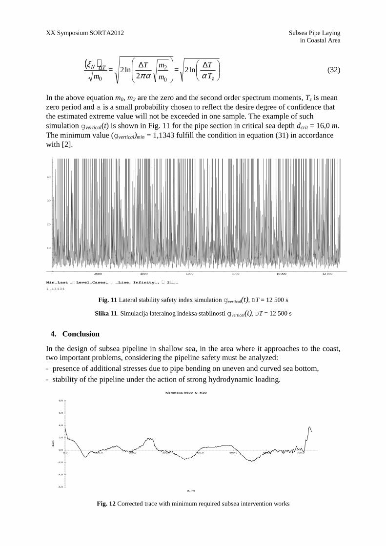
In the above equation m0, m2 are the zero and the second order spectrum moments, Tz is mean zero period and a is a small probability chosen to reflect the desire degree of confidence that the estimated extreme value will not be exceeded in one sample. The example of such simulation gvertical(t) is shown in Fig. 11 for the pipe section in critical sea depth dcrit = 16,0 m. The minimum value (gvertical)min = 1,1343 fulfill the condition in equation (31) in accordance with [2].

2000 4000 6000 8000 10000 12 000

10

20

30

40

MinLast LevelCases , _Line, Infinity, 21.13434

Fig. 11 Lateral stability safety index simulation gvertical(t), DT = 12 500 s

Slika 11. Simulacija lateralnog indeksa stabilnosti gvertical(t), DT = 12 500 s

4. Conclusion

In the design of subsea pipeline in shallow sea, in the area where it approaches to the coast, two important problems, considering the pipeline safety must be analyzed:

- presence of additional stresses due to pipe bending on uneven and curved sea bottom,

- stability of the pipeline under the action of strong hydrodynamic loading.

Korekcija R600_C_K30

-6,0

-4,0

-2,0

0,0

2,0

4,0

6,0

8,0

0,0 100,0 200,0 300,0 400,0 500,0 600,0 700,0

x, m

z, m

Fig. 12 Corrected trace with minimum required subsea intervention works


Slika 12. Korigirana trasa sa minimalnim zahtijevanim podmorskim radovima

The problems are interrelated and a reliable numerical model has to be applied to find the optimum solution to ensure the required safety with minimum subsea intervention works. The analysis includes the nonlinear FEM model with large displacement/small deformations including contact problem, in deterministic domain, and model of the design sea state and wave loading, in probabilistic domain.

93,33; -16,00 695,66; -16,00

157,31; -20,0683,591; -20,0

-60,0

-50,0

-40,0

-30,0

-20,0

-10,0

0,0

0,0 50,0 100,0 150,0 200,0 250,0 300,0 350,0 400,0 450,0 500,0 550,0 600,0 650,0 700,0 750,0

x m

z m

Nezaštičeni cjevovod na morskom dnu

Zaštičeni cjevovod na morskom dnu

Zaštičeni cjevovod na morskom dnu

LP1(0.0; 0,9) LP2(733,38;0,70)

DNV-RP-F109

HRH ENV

DNV-OS-F101,

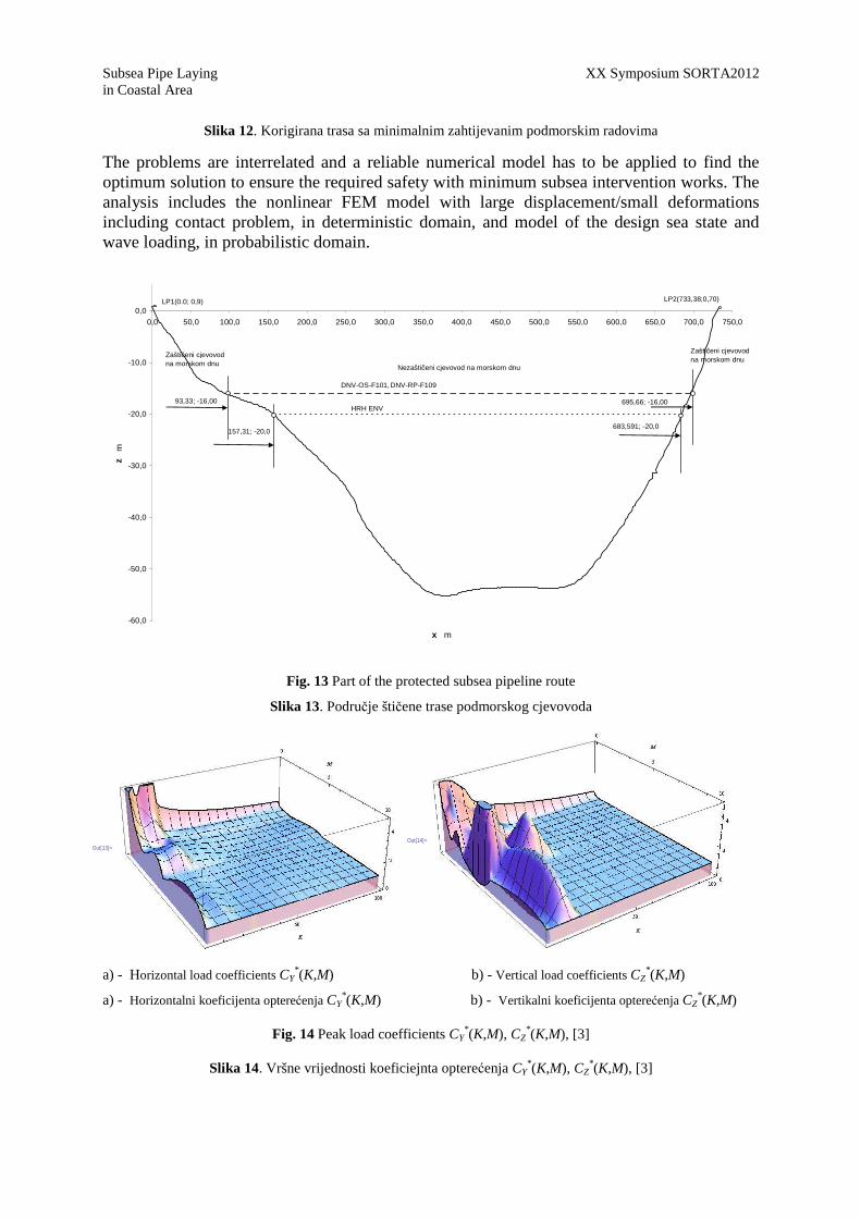
Fig. 13 Part of the protected subsea pipeline route

Slika 13. Područje štičene trase podmorskog cjevovoda

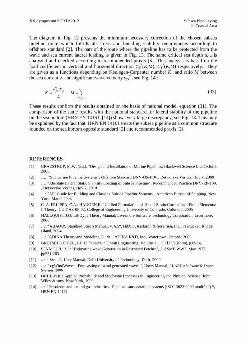
a) - Horizontal load coefficients CY*(K,M) b) - Vertical load coefficients CZ

*(K,M)

a) - Horizontalni koeficijenta opterećenja CY*(K,M) b) - Vertikalni koeficijenta opterećenja CZ

*(K,M)

Fig. 14 Peak load coefficients CY*(K,M), CZ

*(K,M), [3]

Slika 14. Vršne vrijednosti koeficiejnta opterećenja CY*(K,M), CZ

*(K,M), [3]

Out[14]=Out[13]=


The diagram in Fig. 12 presents the minimum necessary correction of the chosen subsea pipeline route which fulfills all stress and buckling stability requirements according to offshore standard [2]. The part of the route where the pipeline has to be protected from the wave and sea current lateral loading is given in Fig. 13. The same critical sea depth dcrit is analyzed and checked according to recommended praxis [3]. This analysis is based on the load coefficient in vertical and horizontal direction CZ

*(K,M), CY*(K,M) respectively. They

are given as a functions depending on Keulegan-Carpenter number K and ratio M between the sea current vc and significant wave velocity vys

* , see Fig. 14 :

*

*

;ys

cpys

v

vM

D

TvK == (33)

These results confirm the results obtained on the basis of rational model, equation (31). The comparison of the same results with the national standard for lateral stability of the pipeline on the sea bottom (HRN EN 14161, [14]) shows very large discrepancy, see Fig. 13. This may be explained by the fact that HRN EN 14161 treats the subsea pipeline as a common structure founded on the sea bottom opposite standard [2] and recommended praxis [3].

REFERENCES

[1] BRAESTRUP, M.W. (Ed.): "Design and Installation of Marine Pipelines; Blackwell Science Ltd, Oxford, 2005

[2] ….: "Submarine Pipeline Systems", Offshore Standard DNV-OS-F101, Det norske Veritas, Høvik, 2000

[3] …: "Absolute Lateral Static Stability Loading of Subsea Pipeline", Recommended Practice DNV-RP-109, , Det norske Veritas, Høvik, 2010

[4] …: "API Guide for Building and Classing Subsea Pipeline Systems", American Bureau of Shipping, New York, March 2004

[5] C. A. FELIPPA, C.A.: HAUGEN,B: "Unified Formulation of Small-Strain Corotational Finite Elements: I. Theory: CU-CAS-05-02: College of Engineering University of Colorado: Colorado, 2005

[6] HALLQUIST;J.O: LS-Dyna Theory Manual; Livermore Software Technology Corporation, Livermore, 2006

[7] …: “ ABAQUS/Standard User’s Manual, v. 6.5“, Hibbitt, Karlsson & Sorensen, Inc., Pawtucket, Rhode Island, 2004.

[8] …: "ADINA Theory and Modeling Guide“, ADINA R&D, Inc., Watertown, October 2005

[9] BRETSCHNEIDER, CH.I.: "Topics in Ocean Engineering, Volume 1", Gulf Publishing, p32-34,

[10] SEYMOUR, R.J.: "Estimating wave Generation in Restricted Fetches", J. ASME WW2, May 1977, pp251-263.

[11] ...: “ Swan“, User Manual, Delft University of Technology, Delft, 2009

[12] …: " cgWindWaves - Forecasting of wind generated waves ", Users Manual, RUNET ®Software & Expert Systems, 2006

[13] OCHI, M.K.: Applied Probability and Stochastic Processes in Engineering and Physical Science, John Wiley & sons, New York, 1990

[14] ...: “ Petroleum and natural gas industries - Pipeline transportation systems (ISO 13623:2000 modified) “, HRN EN 14161

SUBSEA PIPE LAYING IN COASTAL AREA - hrbi.hr · SUBSEA PIPE LAYING IN COASTAL AREA ... morskog dna...

Documents

Transcript of SUBSEA PIPE LAYING IN COASTAL AREA - hrbi.hr · SUBSEA PIPE LAYING IN COASTAL AREA ... morskog dna...