Study Guide: Finite difference methods for wave

motion

Hans Petter Langtangen1,2

1Center for Biomedical Computing, Simula Research Laboratory2Department of Informatics, University of Oslo

Dec 12, 2013

Contents

1 Finite difference methods for waves on a string 11.1 The complete initial-boundary value problem . . . . . . . . . . . . . . . . . . . . 11.2 Input data in the problem . . . . . . . . . . . . . . . . . . . . . . . . . . . . . . . 21.3 Demo of a vibrating string (C = 0.8) . . . . . . . . . . . . . . . . . . . . . . . . . 21.4 Demo of a vibrating string (C = 1.0012) . . . . . . . . . . . . . . . . . . . . . . . 21.5 Step 1: Discretizing the domain . . . . . . . . . . . . . . . . . . . . . . . . . . . . 21.6 The discrete solution . . . . . . . . . . . . . . . . . . . . . . . . . . . . . . . . . . 31.7 Step 2: Fulfilling the equation at the mesh points . . . . . . . . . . . . . . . . . . 31.8 Step 3: Replacing derivatives by finite differences . . . . . . . . . . . . . . . . . . 31.9 Step 3: Algebraic version of the PDE . . . . . . . . . . . . . . . . . . . . . . . . . 41.10 Step 3: Algebraic version of the initial conditions . . . . . . . . . . . . . . . . . . 41.11 Step 4: Formulating a recursive algorithm . . . . . . . . . . . . . . . . . . . . . . 41.12 The Courant number . . . . . . . . . . . . . . . . . . . . . . . . . . . . . . . . . . 41.13 The finite difference stencil . . . . . . . . . . . . . . . . . . . . . . . . . . . . . . 51.14 The stencil for the first time level . . . . . . . . . . . . . . . . . . . . . . . . . . . 51.15 The algorithm . . . . . . . . . . . . . . . . . . . . . . . . . . . . . . . . . . . . . . 51.16 Moving finite difference stencil . . . . . . . . . . . . . . . . . . . . . . . . . . . . 61.17 Sketch of an implementation (1) . . . . . . . . . . . . . . . . . . . . . . . . . . . 61.18 PDE solvers should save memory . . . . . . . . . . . . . . . . . . . . . . . . . . . 61.19 Sketch of an implementation (2) . . . . . . . . . . . . . . . . . . . . . . . . . . . 6

2 Verification 72.1 A slightly generalized model problem . . . . . . . . . . . . . . . . . . . . . . . . . 72.2 Discrete model for the generalized model problem . . . . . . . . . . . . . . . . . . 72.3 Modified equation for the first time level . . . . . . . . . . . . . . . . . . . . . . . 72.4 Using an analytical solution of physical significance . . . . . . . . . . . . . . . . . 82.5 Manufactured solution: principles . . . . . . . . . . . . . . . . . . . . . . . . . . . 82.6 Manufactured solution: example . . . . . . . . . . . . . . . . . . . . . . . . . . . 82.7 Testing a manufactured solution . . . . . . . . . . . . . . . . . . . . . . . . . . . 9

2.8 Constructing an exact solution of the discrete equations . . . . . . . . . . . . . . 92.9 Analytical work with the PDE problem . . . . . . . . . . . . . . . . . . . . . . . 92.10 Analytical work with the discrete equations (1) . . . . . . . . . . . . . . . . . . . 92.11 Analytical work with the discrete equations (1) . . . . . . . . . . . . . . . . . . . 102.12 Testing with the exact discrete solution . . . . . . . . . . . . . . . . . . . . . . . 10

3 Implementation 103.1 The algorithm . . . . . . . . . . . . . . . . . . . . . . . . . . . . . . . . . . . . . . 103.2 What do to with the solution? . . . . . . . . . . . . . . . . . . . . . . . . . . . . 103.3 Making a solver function (1) . . . . . . . . . . . . . . . . . . . . . . . . . . . . . . 113.4 Making a solver function (2) . . . . . . . . . . . . . . . . . . . . . . . . . . . . . . 113.5 Verification: exact quadratic solution . . . . . . . . . . . . . . . . . . . . . . . . . 123.6 Visualization: animating u(x, t) . . . . . . . . . . . . . . . . . . . . . . . . . . . . 123.7 Making movie files . . . . . . . . . . . . . . . . . . . . . . . . . . . . . . . . . . . 133.8 Running a case . . . . . . . . . . . . . . . . . . . . . . . . . . . . . . . . . . . . . 143.9 Implementation of the case . . . . . . . . . . . . . . . . . . . . . . . . . . . . . . 143.10 Resulting movie for C = 0.8 . . . . . . . . . . . . . . . . . . . . . . . . . . . . . . 143.11 The benefits of scaling . . . . . . . . . . . . . . . . . . . . . . . . . . . . . . . . . 14

4 Vectorization 154.1 Operations on slices of arrays . . . . . . . . . . . . . . . . . . . . . . . . . . . . . 154.2 Test the understanding . . . . . . . . . . . . . . . . . . . . . . . . . . . . . . . . . 164.3 Vectorization of finite difference schemes (1) . . . . . . . . . . . . . . . . . . . . . 164.4 Vectorization of finite difference schemes (2) . . . . . . . . . . . . . . . . . . . . . 164.5 Vectorized implementation in the solver function . . . . . . . . . . . . . . . . . . 164.6 Verification of the vectorized version . . . . . . . . . . . . . . . . . . . . . . . . . 174.7 Efficiency measurements . . . . . . . . . . . . . . . . . . . . . . . . . . . . . . . . 17

5 Generalization: reflecting boundaries 185.1 Neumann boundary condition . . . . . . . . . . . . . . . . . . . . . . . . . . . . . 185.2 Discretization of derivatives at the boundary (1) . . . . . . . . . . . . . . . . . . 185.3 Discretization of derivatives at the boundary (2) . . . . . . . . . . . . . . . . . . 185.4 Visualization of modified boundary stencil . . . . . . . . . . . . . . . . . . . . . . 195.5 Implementation of Neumann conditions . . . . . . . . . . . . . . . . . . . . . . . 195.6 Moving finite difference stencil . . . . . . . . . . . . . . . . . . . . . . . . . . . . 195.7 Index set notation . . . . . . . . . . . . . . . . . . . . . . . . . . . . . . . . . . . 195.8 Index set notation in code . . . . . . . . . . . . . . . . . . . . . . . . . . . . . . . 205.9 Index sets in action (1) . . . . . . . . . . . . . . . . . . . . . . . . . . . . . . . . . 205.10 Index sets in action (2) . . . . . . . . . . . . . . . . . . . . . . . . . . . . . . . . . 205.11 Alternative implementation via ghost cells . . . . . . . . . . . . . . . . . . . . . . 215.12 Implementation of ghost cells (1) . . . . . . . . . . . . . . . . . . . . . . . . . . . 215.13 Implementation of ghost cells (2) . . . . . . . . . . . . . . . . . . . . . . . . . . . 21

6 Generalization: variable wave velocity 226.1 The model PDE with a variable coefficient . . . . . . . . . . . . . . . . . . . . . . 226.2 Discretizing the variable coefficient (1) . . . . . . . . . . . . . . . . . . . . . . . . 226.3 Discretizing the variable coefficient (2) . . . . . . . . . . . . . . . . . . . . . . . . 226.4 Discretizing the variable coefficient (3) . . . . . . . . . . . . . . . . . . . . . . . . 236.5 Computing the coefficient between mesh points . . . . . . . . . . . . . . . . . . . 236.6 Discretization of variable-coefficient wave equation in operator notation . . . . . 23

2

6.7 Neumann condition and a variable coefficient . . . . . . . . . . . . . . . . . . . . 24

6.8 Implementation of variable coefficients . . . . . . . . . . . . . . . . . . . . . . . . 24

6.9 A more general model PDE with variable coefficients . . . . . . . . . . . . . . . . 24

6.10 Generalization: damping . . . . . . . . . . . . . . . . . . . . . . . . . . . . . . . . 25

7 Building a general 1D wave equation solver 25

7.1 Collection of initial conditions . . . . . . . . . . . . . . . . . . . . . . . . . . . . . 25

8 Finite difference methods for 2D and 3D wave equations 26

8.1 Examples on wave equations written out in 2D/3D . . . . . . . . . . . . . . . . . 26

8.2 Boundary and initial conditions . . . . . . . . . . . . . . . . . . . . . . . . . . . . 26

8.3 Example: 2D propagation of Gaussian function . . . . . . . . . . . . . . . . . . . 27

8.4 Mesh . . . . . . . . . . . . . . . . . . . . . . . . . . . . . . . . . . . . . . . . . . . 27

8.5 Discretization . . . . . . . . . . . . . . . . . . . . . . . . . . . . . . . . . . . . . . 27

8.6 Special stencil for the first time step . . . . . . . . . . . . . . . . . . . . . . . . . 27

8.7 Variable coefficients (1) . . . . . . . . . . . . . . . . . . . . . . . . . . . . . . . . 27

8.8 Variable coefficients (2) . . . . . . . . . . . . . . . . . . . . . . . . . . . . . . . . 28

8.9 Neumann boundary condition in 2D . . . . . . . . . . . . . . . . . . . . . . . . . 28

9 Implementation of 2D/3D problems 28

9.1 Algorithm . . . . . . . . . . . . . . . . . . . . . . . . . . . . . . . . . . . . . . . . 29

9.2 Scalar computations: mesh . . . . . . . . . . . . . . . . . . . . . . . . . . . . . . 29

9.3 Scalar computations: arrays . . . . . . . . . . . . . . . . . . . . . . . . . . . . . . 29

9.4 Scalar computations: initial condition . . . . . . . . . . . . . . . . . . . . . . . . 29

9.5 Scalar computations: primary stencil . . . . . . . . . . . . . . . . . . . . . . . . . 30

9.6 Vectorized computations: mesh coordinates . . . . . . . . . . . . . . . . . . . . . 30

9.7 Vectorized computations: stencil . . . . . . . . . . . . . . . . . . . . . . . . . . . 30

9.8 Verification: quadratic solution (1) . . . . . . . . . . . . . . . . . . . . . . . . . . 31

9.9 Verification: quadratic solution (2) . . . . . . . . . . . . . . . . . . . . . . . . . . 31

10 Migrating loops to Cython 31

10.1 Declaring variables and annotating the code . . . . . . . . . . . . . . . . . . . . . 32

10.2 Cython version of the functions . . . . . . . . . . . . . . . . . . . . . . . . . . . . 32

10.3 Visual inspection of the C translation . . . . . . . . . . . . . . . . . . . . . . . . 32

10.4 Building the extension module . . . . . . . . . . . . . . . . . . . . . . . . . . . . 33

10.5 Calling the Cython function from Python . . . . . . . . . . . . . . . . . . . . . . 34

11 Migrating loops to Fortran 34

11.1 The Fortran subroutine . . . . . . . . . . . . . . . . . . . . . . . . . . . . . . . . 34

11.2 Building the Fortran module with f2py . . . . . . . . . . . . . . . . . . . . . . . . 35

11.3 How to avoid array copying . . . . . . . . . . . . . . . . . . . . . . . . . . . . . . 35

11.4 Efficiency of translating to Fortran . . . . . . . . . . . . . . . . . . . . . . . . . . 35

12 Migrating loops to C via Cython 36

12.1 The C code . . . . . . . . . . . . . . . . . . . . . . . . . . . . . . . . . . . . . . . 36

12.2 The Cython interface file . . . . . . . . . . . . . . . . . . . . . . . . . . . . . . . . 36

12.3 Building the extension module . . . . . . . . . . . . . . . . . . . . . . . . . . . . 37

3

13 Migrating loops to C via f2py 37

13.1 The C code and the Fortran interface file . . . . . . . . . . . . . . . . . . . . . . 37

13.2 Building the extension module . . . . . . . . . . . . . . . . . . . . . . . . . . . . 38

13.3 Migrating loops to C++ via f2py . . . . . . . . . . . . . . . . . . . . . . . . . . . 38

14 Analysis of the difference equations 38

14.1 Properties of the solution of the wave equation . . . . . . . . . . . . . . . . . . . 38

14.2 Demo of the splitting of I(x) into two waves . . . . . . . . . . . . . . . . . . . . . 39

14.3 Effect of variable wave velocity . . . . . . . . . . . . . . . . . . . . . . . . . . . . 39

14.4 What happens here? . . . . . . . . . . . . . . . . . . . . . . . . . . . . . . . . . . 39

14.5 Representation of waves as sum of sine/cosine waves . . . . . . . . . . . . . . . . 39

14.6 Analysis of the finite difference scheme . . . . . . . . . . . . . . . . . . . . . . . . 40

14.7 Preliminary results . . . . . . . . . . . . . . . . . . . . . . . . . . . . . . . . . . . 40

14.8 Numerical wave propagation (1) . . . . . . . . . . . . . . . . . . . . . . . . . . . 40

14.9 Numerical wave propagation (2) . . . . . . . . . . . . . . . . . . . . . . . . . . . 40

14.10Numerical wave propagation (3) . . . . . . . . . . . . . . . . . . . . . . . . . . . 41

14.11Why C ≤ 1 is a stability criterion . . . . . . . . . . . . . . . . . . . . . . . . . . . 41

14.12Numerical dispersion relation . . . . . . . . . . . . . . . . . . . . . . . . . . . . . 41

14.13The special case C = 1 . . . . . . . . . . . . . . . . . . . . . . . . . . . . . . . . . 42

14.14Computing the error in wave velocity . . . . . . . . . . . . . . . . . . . . . . . . . 42

14.15Visualizing the error in wave velocity . . . . . . . . . . . . . . . . . . . . . . . . . 42

14.16Taylor expanding the error in wave velocity . . . . . . . . . . . . . . . . . . . . . 43

14.17Example on effect of wrong wave velocity (1) . . . . . . . . . . . . . . . . . . . . 43

14.18Example on effect of wrong wave velocity (1) . . . . . . . . . . . . . . . . . . . . 43

14.19Extending the analysis to 2D (and 3D) . . . . . . . . . . . . . . . . . . . . . . . . 44

14.20Discrete wave components in 2D . . . . . . . . . . . . . . . . . . . . . . . . . . . 44

14.21Stability criterion in 2D . . . . . . . . . . . . . . . . . . . . . . . . . . . . . . . . 44

14.22Stability criterion in 3D . . . . . . . . . . . . . . . . . . . . . . . . . . . . . . . . 45

14.23Numerical dispersion relation in 2D (1) . . . . . . . . . . . . . . . . . . . . . . . 45

14.24Numerical dispersion relation in 2D (2) . . . . . . . . . . . . . . . . . . . . . . . 45

14.25Numerical dispersion relation in 2D (3) . . . . . . . . . . . . . . . . . . . . . . . 46

1 Finite difference methods for waves on a string

Waves on a string can be modeled by the wave equation

∂2u

∂t2= c2

∂2u

∂x2

u(x, t) is the displacement of the string

Demo of waves on a string1.

1http://phet.colorado.edu/sims/wave-on-a-string/wave-on-a-string en.html

4

1.1 The complete initial-boundary value problem

∂2u

∂t2= c2

∂2u

∂x2, x ∈ (0, L), t ∈ (0, T ] (1)

u(x, 0) = I(x), x ∈ [0, L] (2)

∂

∂tu(x, 0) = 0, x ∈ [0, L] (3)

u(0, t) = 0, t ∈ (0, T ] (4)

u(L, t) = 0, t ∈ (0, T ] (5)

1.2 Input data in the problem

• Initial condition u(x, 0) = I(x): initial string shape

• Initial condition ut(x, 0) = 0: string starts from rest

• c =√T/%: velocity of waves on the string

• (T is the tension in the string, % is density of the string)

• Two boundary conditions on u: u = 0 means fixed ends (no displacement)

Rule for number of initial and boundary conditions:

• utt in the PDE: two initial conditions, on u and ut

• ut (and no utt) in the PDE: one initial conditions, on u

• uxx in the PDE: one boundary condition on u at each boundary point

1.3 Demo of a vibrating string (C = 0.8)

• Our numerical method is sometimes exact (!)

• Our numerical method is sometimes subject to serious non-physical effects

1.4 Demo of a vibrating string (C = 1.0012)

Ooops!

1.5 Step 1: Discretizing the domain

Mesh in time:

0 = t0 < t1 < t2 < · · · < tNt−1 < tNt= T (6)

Mesh in space:

0 = x0 < x1 < x2 < · · · < xNx−1 < xNx = L (7)

Uniform mesh with constant mesh spacings ∆t and ∆x:

xi = i∆x, i = 0, . . . , Nx, ti = n∆t, n = 0, . . . , Nt (8)

5

1.6 The discrete solution

• The numerical solution is a mesh function: uni ≈ ue(xi, tn)

• Finite difference stencil (or scheme): equation for uni involving neighboring space-timepoints

0

1

2

3

4

5

0 1 2 3 4 5

inde

x n

index i

Stencil at interior point

1.7 Step 2: Fulfilling the equation at the mesh points

Let the PDE be satisfied at all interior mesh points:

∂2

∂t2u(xi, tn) = c2

∂2

∂x2u(xi, tn), (9)

for i = 1, . . . , Nx − 1 and n = 1, . . . , Nt − 1.For n = 0 we have the initial conditions u = I(x) and ut = 0, and at the boundaries i = 0, Nx

we have the boundary condition u = 0.

1.8 Step 3: Replacing derivatives by finite differences

Widely used finite difference formula for the second-order derivative:

∂2

∂t2u(xi, tn) ≈ un+1

i − 2uni + un−1i

∆t2= [DtDtu]ni

and

∂2

∂x2u(xi, tn) ≈

uni+1 − 2uni + uni−1

∆x2= [DxDxu]ni

6

1.9 Step 3: Algebraic version of the PDE

Replace derivatives by differences:

un+1i − 2uni + un−1

i

∆t2= c2

uni+1 − 2uni + uni−1

∆x2, (10)

In operator notation:

[DtDtu = c2DxDx]ni (11)

1.10 Step 3: Algebraic version of the initial conditions

• Need to replace the derivative in the initial condition ut(x, 0) = 0 by a finite differenceapproximation

• The differences for utt and uxx have second-order accuracy

• Use a centered difference for ut(x, 0)

[D2tu]ni = 0, n = 0 ⇒ un−1i = un+1

i , i = 0, . . . , Nx

The other initial condition u(x, 0) = I(x) can be computed by

u0i = I(xi), i = 0, . . . , Nx

1.11 Step 4: Formulating a recursive algorithm

• Nature of the algorithm: compute u in space at t = ∆t, 2∆t, 3∆t, ...

• Three time levels are involved in the general discrete equation: n+ 1, n, n− 1

• uni and un−1i are then already computed for i = 0, . . . , Nx, and un+1

i is the unknown quantity

Write out [DtDtu = c2DxDx]ni and solve for un+1i ,

un+1i = −un−1

i + 2uni + C2(uni+1 − 2uni + uni−1

)(12)

1.12 The Courant number

C = c∆t

∆x, (13)

is known as the (dimensionless) Courant number

Notice.There is only one parameter, C, in the discrete model: C lumps mesh parameters with thewave velocity c. The value C and the smoothness of I(x) govern the quality of the numericalsolution.

7

1.13 The finite difference stencil

0

1

2

3

4

5

0 1 2 3 4 5

inde

x n

index i

Stencil at interior point

1.14 The stencil for the first time level

• Problem: the stencil for n = 1 involves u−1i , but time t = −∆t is outside the mesh

• Remedy: use the initial condition ut = 0 together with the stencil to eliminate u−1i

Initial condition:

[D2tu = 0]0i ⇒ u−1i = u1

i

Insert in stencil [DtDtu = c2DxDx]0i to get

u1i = u0

i −1

2C2(uni+1 − 2uni + uni−1

)(14)

1.15 The algorithm

1. Compute u0i = I(xi) for i = 0, . . . , Nx

2. Compute u1i by (14) and set u1

i = 0 for the boundary points i = 0 and i = Nx, forn = 1, 2, . . . , N − 1,

3. For each time level n = 1, 2, . . . , Nt − 1

(a) apply (12) to find un+1i for i = 1, . . . , Nx − 1

(b) set un+1i = 0 for the boundary points i = 0, i = Nx.

8

1.16 Moving finite difference stencil

web page2 or a movie file3.

1.17 Sketch of an implementation (1)

• Arrays:

– u[i] stores un+1i

– u_1[i] stores uni

– u_2[i] stores un−1i

Naming convention.

u is the unknown to be computed (a spatial mesh function), u_k is the computed spatialmesh function k time steps back in time.

1.18 PDE solvers should save memory

Important to minimize the memory usage.

The algorithm only needs to access the three most recent time levels, so we need only threearrays for un+1

i , uni , and un−1i , i = 0, . . . , Nx. Storing all the solutions in a two-dimensional

array of size (Nx + 1) × (Nt + 1) would be possible in this simple one-dimensional PDEproblem, but not in large 2D problems and not even in small 3D problems.

1.19 Sketch of an implementation (2)

# Given mesh points as arrays x and t (x[i], t[n])dx = x[1] - x[0]dt = t[1] - t[0]C = c*dt/dx # Courant numberNt = len(t)-1C2 = C**2 # Help variable in the scheme

# Set initial condition u(x,0) = I(x)for i in range(0, Nx+1):

u_1[i] = I(x[i])

# Apply special formula for first step, incorporating du/dt=0for i in range(1, Nx):

u[i] = u_1[i] - 0.5*C**2(u_1[i+1] - 2*u_1[i] + u_1[i-1])u[0] = 0; u[Nx] = 0 # Enforce boundary conditions

# Switch variables before next stepu_2[:], u_1[:] = u_1, u

for n in range(1, Nt):# Update all inner mesh points at time t[n+1]for i in range(1, Nx):

u[i] = 2u_1[i] - u_2[i] - \C**2(u_1[i+1] - 2*u_1[i] + u_1[i-1])

2http://tinyurl.com/k3sdbuv/pub/mov-wave/wave1D PDE Dirichlet stencil gpl/index.html3http://tinyurl.com/k3sdbuv/pub/mov-wave/wave1D PDE Dirichlet stencil gpl/movie.ogg

9

# Insert boundary conditionsu[0] = 0; u[Nx] = 0

# Switch variables before next stepu_2[:], u_1[:] = u_1, u

2 Verification

• Think about testing and verification before you start implementing the algorithm!

• Powerful testing tool: method of manufactured solutions and computation of convergencerates

• Will need a source term in the PDE and ut(x, 0) 6= 0

• Even more powerful method: exact solution of the scheme

2.1 A slightly generalized model problem

Add source term f and nonzero initial condition ut(x, 0):

utt = c2uxx + f(x, t), (15)

u(x, 0) = I(x), x ∈ [0, L] (16)

ut(x, 0) = V (x), x ∈ [0, L] (17)

u(0, t) = 0, t > 0, (18)

u(L, t) = 0, t > 0 (19)

2.2 Discrete model for the generalized model problem

[DtDtu = c2DxDx + f ]ni (20)

Writing out and solving for the unknown un+1i :

un+1i = −un−1

i + 2uni + C2(uni+1 − 2uni + uni−1) + ∆t2fni (21)

2.3 Modified equation for the first time level

Centered difference for ut(x, 0) = V (x):

[D2tu = V ]0i ⇒ u−1i = u1

i − 2∆tVi,

Inserting this in the stencil (21) for n = 0 leads to

u1i = u0

i −∆tVi +1

2C2(uni+1 − 2uni + uni−1

)+

1

2∆t2fni (22)

10

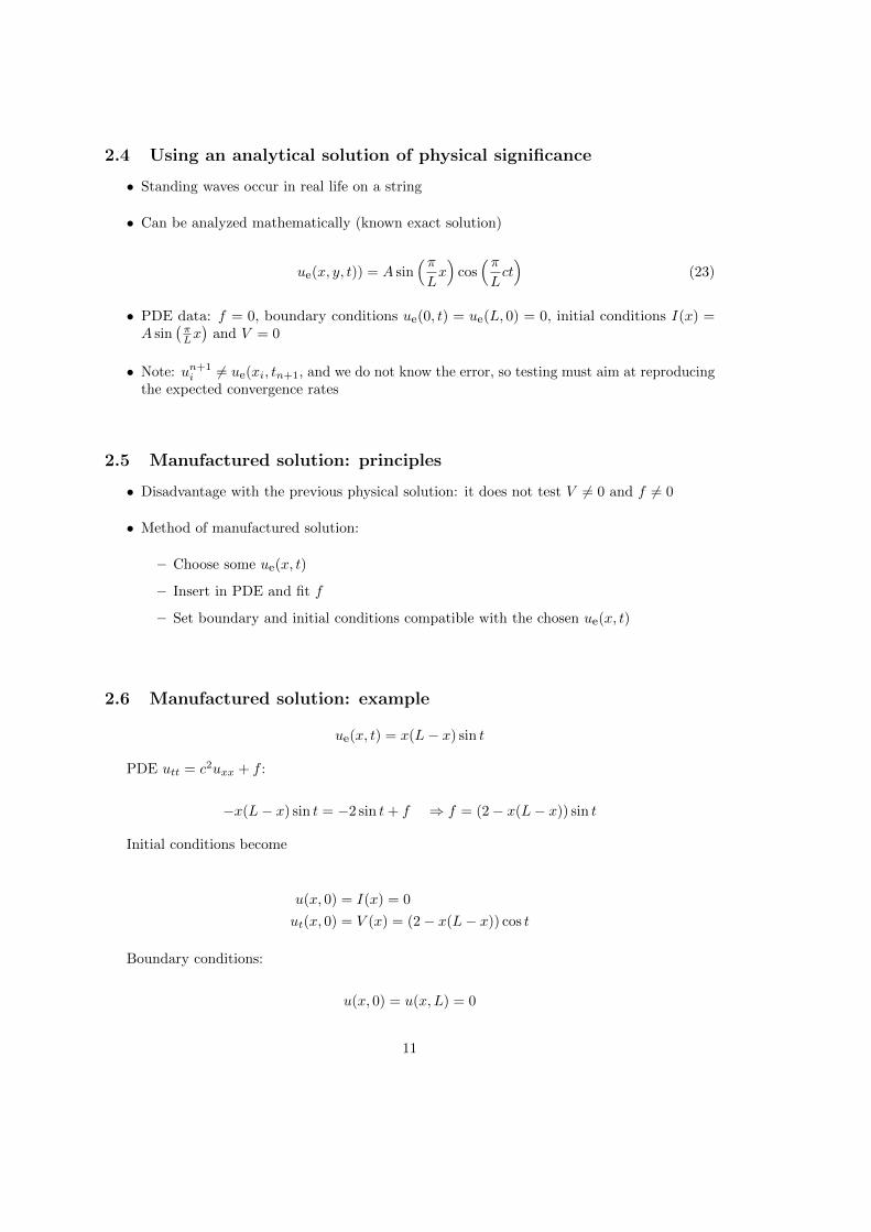
2.4 Using an analytical solution of physical significance

• Standing waves occur in real life on a string

• Can be analyzed mathematically (known exact solution)

ue(x, y, t)) = A sin(πLx)

cos(πLct)

(23)

• PDE data: f = 0, boundary conditions ue(0, t) = ue(L, 0) = 0, initial conditions I(x) =A sin

(πLx)

and V = 0

• Note: un+1i 6= ue(xi, tn+1, and we do not know the error, so testing must aim at reproducing

the expected convergence rates

2.5 Manufactured solution: principles

• Disadvantage with the previous physical solution: it does not test V 6= 0 and f 6= 0

• Method of manufactured solution:

– Choose some ue(x, t)

– Insert in PDE and fit f

– Set boundary and initial conditions compatible with the chosen ue(x, t)

2.6 Manufactured solution: example

ue(x, t) = x(L− x) sin t

PDE utt = c2uxx + f :

−x(L− x) sin t = −2 sin t+ f ⇒ f = (2− x(L− x)) sin t

Initial conditions become

u(x, 0) = I(x) = 0

ut(x, 0) = V (x) = (2− x(L− x)) cos t

Boundary conditions:

u(x, 0) = u(x, L) = 0

11

2.7 Testing a manufactured solution

• Introduce common mesh parameter: h = ∆t, ∆x = ch/C

• This h keeps C and ∆t/∆x constant

• Select coarse mesh h: h0

• Run experiments with hi = 2−ih0 (halving the cell size), i = 0, . . . ,m

• Record the error Ei and hi in each experiment

• Compute pariwise convergence rates ri = lnEi+1/Ei/ lnhi+1/hi

• Verification: ri → 2 as i increases

2.8 Constructing an exact solution of the discrete equations

• Manufactured solution with computation of convergence rates: much manual work

• Simpler and more powerful: use an exact solution for uni

• A linear or quadratic ue in x and t is often a good candidate

2.9 Analytical work with the PDE problem

Here, choose ue such that ue(x, 0) = ue(L, 0) = 0:

ue(x, t) = x(L− x)(1 +1

2t),

Insert in the PDE and find f :

f(x, t) = 2(1 + t)c2

Initial conditions:

I(x) = x(L− x), V (x) =1

2x(L− x)

2.10 Analytical work with the discrete equations (1)

We want to show that ue also solves the discrete equations!Useful preliminary result:

[DtDtt2]n =

t2n+1 − 2t2n + t2n−1

∆t2= (n+ 1)2 − n2 + (n− 1)2 = 2 (24)

[DtDtt]n =

tn+1 − 2tn + tn−1

∆t2=

((n+ 1)− n+ (n− 1))∆t

∆t2= 0 (25)

Hence,

[DtDtue]ni = xi(L− xi)[DtDt(1 +

1

2t)]n = xi(L− xi)

1

2[DtDtt]

n = 0

12

2.11 Analytical work with the discrete equations (1)

[DxDxue]ni = (1 +

1

2tn)[DxDx(xL− x2)]i = (1 +

1

2tn)[LDxDxx−DxDxx

2]i

= −2(1 +1

2tn)

Now, fni = 2(1 + 12 tn)c2 and we get

[DtDtue − c2DxDxue − f ]ni = 0− c2(−1)2(1 +1

2tn + 2(1 +

1

2tn)c2 = 0

Moreover, ue(xi, 0) = I(xi), ∂ue/∂t = V (xi) at t = 0, and ue(x0, t) = ue(xNx , 0) = 0. Alsothe modified scheme for the first time step is fulfilled by ue(xi, tn).

2.12 Testing with the exact discrete solution

• We have established that un+1i = ue(xi, tn+1) = xi(L− xi)(1 + tn+1/2)

• Run one simulation with one choice of c, ∆t, and ∆x

• Check that maxi |un+1i − ue(xi, tn+1)| < ε, ε ∼ 10−14 (machine precision + some round-off

errors)

• This is the simplest and best verification test

Later we show that the exact solution of the discrete equations can be obtained by C = 1 (!)

3 Implementation

3.1 The algorithm

1. Compute u0i = I(xi) for i = 0, . . . , Nx

2. Compute u1i by (14) and set u1

i = 0 for the boundary points i = 0 and i = Nx, forn = 1, 2, . . . , N − 1,

3. For each time level n = 1, 2, . . . , Nt − 1

(a) apply (12) to find un+1i for i = 1, . . . , Nx − 1

(b) set un+1i = 0 for the boundary points i = 0, i = Nx.

3.2 What do to with the solution?

• Different problem settings demand different actions with the computed un+1i at each time

step

• Solution: let the solver function make a callback to a user function where the user can dowhatever is desired with the solution

• Advantage: solver just solves and user uses the solution

13

def user_action(u, x, t, n):# u[i] at spatial mesh points x[i] at time t[n]# plot u# or store u

3.3 Making a solver function (1)

def solver(I, V, f, c, L, Nx, C, T, user_action=None):"""Solve u_tt=c^2*u_xx + f on (0,L)x(0,T]."""x = linspace(0, L, Nx+1) # Mesh points in spacedx = x[1] - x[0]dt = C*dx/cNt = int(round(T/dt))t = linspace(0, Nt*dt, Nt+1) # Mesh points in timeC2 = C**2 # Help variable in the schemeif f is None or f == 0 :

f = lambda x, t: 0if V is None or V == 0:

V = lambda x: 0

u = zeros(Nx+1) # Solution array at new time levelu_1 = zeros(Nx+1) # Solution at 1 time level backu_2 = zeros(Nx+1) # Solution at 2 time levels back

import time; t0 = time.clock() # for measuring CPU time

# Load initial condition into u_1for i in range(0,Nx+1):

u_1[i] = I(x[i])

if user_action is not None:user_action(u_1, x, t, 0)

3.4 Making a solver function (2)

def solver(I, V, f, c, L, Nx, C, T, user_action=None):...# Special formula for first time stepn = 0for i in range(1, Nx):

u[i] = u_1[i] + dt*V(x[i]) + \0.5*C2*(u_1[i-1] - 2*u_1[i] + u_1[i+1]) + \0.5*dt**2*f(x[i], t[n])

u[0] = 0; u[Nx] = 0

if user_action is not None:user_action(u, x, t, 1)

# Switch variables before next stepu_2[:], u_1[:] = u_1, u

===== Making a solver function (3) =====

\beginshadedquoteBlue\fontsize9pt9pt\beginVerbatimdef solver(I, V, f, c, L, Nx, C, T, user_action=None):

...

14

# Time loop

for n in range(1, Nt):# Update all inner points at time t[n+1]for i in range(1, Nx):

u[i] = - u_2[i] + 2*u_1[i] + \C2*(u_1[i-1] - 2*u_1[i] + u_1[i+1]) + \dt**2*f(x[i], t[n])

# Insert boundary conditionsu[0] = 0; u[Nx] = 0if user_action is not None:

if user_action(u, x, t, n+1):break

# Switch variables before next stepu_2[:], u_1[:] = u_1, u

cpu_time = t0 - time.clock()return u, x, t, cpu_time

3.5 Verification: exact quadratic solution

Exact solution of the PDE problem and the discrete equations: ue(x, t) = x(L− x)(1 + 12 t)

import nose.tools as nt

def test_quadratic():"""Check that u(x,t)=x(L-x)(1+t/2) is exactly reproduced."""def exact_solution(x, t):

return x*(L-x)*(1 + 0.5*t)

def I(x):return exact_solution(x, 0)

def V(x):return 0.5*exact_solution(x, 0)

def f(x, t):return 2*(1 + 0.5*t)*c**2

L = 2.5c = 1.5Nx = 3 # Very coarse meshC = 0.75T = 18

u, x, t, cpu = solver(I, V, f, c, L, Nx, C, T)u_e = exact_solution(x, t[-1])diff = abs(u - u_e).max()nt.assert_almost_equal(diff, 0, places=14)

3.6 Visualization: animating u(x, t)

Make a viz function for animating the curve, with plotting in a user_action function plot_u:

def viz(I, V, f, c, L, Nx, C, T, umin, umax, animate=True):"""Run solver and visualize u at each time level."""import scitools.std as pltimport time, glob, os

15

def plot_u(u, x, t, n):"""user_action function for solver."""plt.plot(x, u, ’r-’,

xlabel=’x’, ylabel=’u’,axis=[0, L, umin, umax],title=’t=%f’ % t[n], show=True)

# Let the initial condition stay on the screen for 2# seconds, else insert a pause of 0.2 s between each plottime.sleep(2) if t[n] == 0 else time.sleep(0.2)plt.savefig(’frame_%04d.png’ % n) # for movie making

# Clean up old movie framesfor filename in glob.glob(’frame_*.png’):

os.remove(filename)

user_action = plot_u if animate else Noneu, x, t, cpu = solver(I, V, f, c, L, Nx, C, T, user_action)

# Make movie filesfps = 4 # Frames per secondplt.movie(’frame_*.png’, encoder=’html’, fps=fps,

output_file=’movie.html’)codec2ext = dict(flv=’flv’, libx64=’mp4’, libvpx=’webm’,

libtheora=’ogg’)filespec = ’frame_%04d.png’movie_program = ’avconv’ # or ’ffmpeg’for codec in codec2ext:

ext = codec2ext[codec]cmd = ’%(movie_program)s -r %(fps)d -i %(filespec)s ’\

’-vcodec %(codec)s movie.%(ext)s’ % vars()os.system(cmd)

Note: plot_u is function inside function and remembers the local variables in viz (known asa closure).

3.7 Making movie files

• Store spatial curve in a file, for each time level

• Name files like ’something_%04d.png’ % frame_counter

• Combine files to a movie

Terminal> scitools movie encoder=html output_file=movie.html \fps=4 frame_*.png # web page with a player

Terminal> avconv -r 4 -i frame_%04d.png -vcodec flv movie.flvTerminal> avconv -r 4 -i frame_%04d.png -vcodec libtheora movie.oggTerminal> avconv -r 4 -i frame_%04d.png -vcodec libx264 movie.mp4Terminal> avconv -r 4 -i frame_%04d.png -vcodec libtheora movie.oggTerminal> avconv -r 4 -i frame_%04d.png -vcodec libpvx movie.webm

Important.

• Zero padding (%04d) is essential for correct sequence of frames in something_*.png

(Unix alphanumeric sort)

• Remove old frame_*.png files before making a new movie

16

3.8 Running a case

• Vibrations of a guitar string

• Triangular initial shape (at rest)

I(x) =

ax/x0, x < x0

a(L− x)/(L− x0), otherwise(26)

Appropriate data:

• L = 75 cm, x0 = 0.8L, a = 5 mm, Nx = 50, time frequency ν = 440 Hz

3.9 Implementation of the case

def guitar(C):"""Triangular wave (pulled guitar string)."""L = 0.75x0 = 0.8*La = 0.005freq = 440wavelength = 2*Lc = freq*wavelengthomega = 2*pi*freqnum_periods = 1T = 2*pi/omega*num_periodsNx = 50

def I(x):return a*x/x0 if x < x0 else a/(L-x0)*(L-x)

umin = -1.2*a; umax = -umincpu = viz(I, 0, 0, c, L, Nx, C, T, umin, umax, animate=True)

Program: wave1D_u0_s.py4.

3.10 Resulting movie for C = 0.8

Movie of the vibrating string5

3.11 The benefits of scaling

• It is difficult to figure out all the physical parameters of a case

• And it is not necessary because of a powerful: scaling

Introduce new x, t, and u without dimension:

x =x

L, t =

c

Lt, u =

u

a

4http://tinyurl.com/jvzzcfn/wave/wave1D u0 s.py5http://tinyurl.com/k3sdbuv/pub/mov-wave/guitar C0.8/index.html

17

Insert this in the PDE (with f = 0) and dropping bars

utt = uxx

Initial condition: set a = 1, L = 1, and x0 ∈ [0, 1] in (26).In the code: set a=c=L=1, x0=0.8, and there is no need to calculate with wavelengths and

frequencies to estimate c!Just one challenge: determine the period of the waves and an appropriate end time (see the

text for details).

4 Vectorization

• Problem: Python loops over long arrays are slow

• One remedy: use vectorized (numpy) code instead of explicit loops

• Other remedies: use Cython, port spatial loops to Fortran or C

• Speedup: 100-1000 (varies with Nx)

Next: vectorized loops

4.1 Operations on slices of arrays

• Introductory example: compute di = ui+1 − ui

n = u.sizefor i in range(0, n-1):

d[i] = u[i+1] - u[i]

• Note: all the differences here are independent of each other.

• Therefore d = (u1, u2, . . . , un)− (u0, u1, . . . , un−1)

• In numpy code: u[1:n] - u[0:n-1] or just u[1:] - u[:-1]

− −−−

0 1 2 3 4

0 1 2 3 4

18

4.2 Test the understanding

Newcomers to vectorization are encouraged to choose a small array u, say with five elements, andsimulate with pen and paper both the loop version and the vectorized version.

4.3 Vectorization of finite difference schemes (1)

Finite difference schemes basically contains differences between array elements with shifted indices.Consider the updating formula

for i in range(1, n-1):u2[i] = u[i-1] - 2*u[i] + u[i+1]

The vectorization consists of replacing the loop by arithmetics on slices of arrays of lengthn-2:

u2 = u[:-2] - 2*u[1:-1] + u[2:]u2 = u[0:n-2] - 2*u[1:n-1] + u[2:n] # alternative

Note: u2 gets length n-2.If u2 is already an array of length n, do update on ”inner” elements

u2[1:-1] = u[:-2] - 2*u[1:-1] + u[2:]u2[1:n-1] = u[0:n-2] - 2*u[1:n-1] + u[2:n] # alternative

4.4 Vectorization of finite difference schemes (2)

Include a function evaluation too:

def f(x):return x**2 + 1

# Scalar versionfor i in range(1, n-1):

u2[i] = u[i-1] - 2*u[i] + u[i+1] + f(x[i])

# Vectorized versionu2[1:-1] = u[:-2] - 2*u[1:-1] + u[2:] + f(x[1:-1])

4.5 Vectorized implementation in the solver function

Scalar loop:

for i in range(1, Nx):u[i] = 2*u_1[i] - u_2[i] + \

C2*(u_1[i-1] - 2*u_1[i] + u_1[i+1])

Vectorized loop:

u[1:-1] = - u_2[1:-1] + 2*u_1[1:-1] + \C2*(u_1[:-2] - 2*u_1[1:-1] + u_1[2:])

or

19

u[1:Nx] = 2*u_1[1:Nx]- u_2[1:Nx] + \C2*(u_1[0:Nx-1] - 2*u_1[1:Nx] + u_1[2:Nx+1])

Program: wave1D_u0_sv.py6

4.6 Verification of the vectorized version

def test_quadratic():"""Check the scalar and vectorized versions work fora quadratic u(x,t)=x(L-x)(1+t/2) that is exactly reproduced."""# The following function must work for x as array or scalarexact_solution = lambda x, t: x*(L - x)*(1 + 0.5*t)I = lambda x: exact_solution(x, 0)V = lambda x: 0.5*exact_solution(x, 0)# f is a scalar (zeros_like(x) works for scalar x too)f = lambda x, t: zeros_like(x) + 2*c**2*(1 + 0.5*t)

L = 2.5c = 1.5Nx = 3 # Very coarse meshC = 1T = 18 # Long time integration

def assert_no_error(u, x, t, n):u_e = exact_solution(x, t[n])diff = abs(u - u_e).max()nt.assert_almost_equal(diff, 0, places=13)

solver(I, V, f, c, L, Nx, C, T,user_action=assert_no_error, version=’scalar’)

solver(I, V, f, c, L, Nx, C, T,user_action=assert_no_error, version=’vectorized’)

Note:

• Compact code with lambda functions

• The scalar f value needs careful coding: return constant array if vectorized code, elsenumber

4.7 Efficiency measurements

• Run wave1D_u0_sv.py for Nx as 50,100,200,400,800 and measuring the CPU time

• Observe substantial speed-up: vectorized version is about Nx/5 times faster

Much bigger improvements for 2D and 3D codes!

6http://tinyurl.com/jvzzcfn/wave/wave1D u0 sv.py

20

5 Generalization: reflecting boundaries

• Boundary condition u = 0: u changes sign

• Boundary condition ux = 0: wave is perfectly reflected

• How can we implement ux? (more complicated than u = 0)

Demo of boundary conditions7

5.1 Neumann boundary condition

∂u

∂n≡ n · ∇u = 0 (27)

For a 1D domain [0, L]:

∂

∂n

∣∣∣∣x=L

=∂

∂x,

∂

∂n

∣∣∣∣x=0

= − ∂

∂x

Boundary condition terminology:

• ux specified: Neumann8 condition

• u specified: Dirichlet9 condition

5.2 Discretization of derivatives at the boundary (1)

• How can we incorporate the condition ux = 0 in the finite difference scheme?

• We used centeral differences for utt and uxx: O(∆t2,∆x2) accuracy

• Also for ut(x, 0)

• Should use central difference for ux to preserve second order accuracy

un−1 − un12∆x

= 0 (28)

5.3 Discretization of derivatives at the boundary (2)

un−1 − un12∆x

= 0

• Problem: un−1 is outside the mesh (fictitious value)

• Remedy: use the stencil at the boundary to eliminate un−1; just replace un−1 by un1

un+1i = −un−1

i + 2uni + 2C2(uni+1 − uni

), i = 0 (29)

7http://phet.colorado.edu/sims/wave-on-a-string/wave-on-a-string en.html8http://en.wikipedia.org/wiki/Neumann boundary condition9http://en.wikipedia.org/wiki/Dirichlet conditions

21

5.4 Visualization of modified boundary stencil

Discrete equation for computing u30 in terms of u2

0, u10, and u2

1:Animation in a web page10 or a movie file11.

5.5 Implementation of Neumann conditions

• Use the general stencil for interior points also on the boundary

• Replace uni−1 by uni+1 for i = 0

• Replace uni+1 by uni−1 for i = Nx

i = 0ip1 = i+1im1 = ip1 # i-1 -> i+1u[i] = u_1[i] + C2*(u_1[im1] - 2*u_1[i] + u_1[ip1])

i = Nxim1 = i-1ip1 = im1 # i+1 -> i-1u[i] = u_1[i] + C2*(u_1[im1] - 2*u_1[i] + u_1[ip1])

# Or just one loop over all points

for i in range(0, Nx+1):ip1 = i+1 if i < Nx else i-1im1 = i-1 if i > 0 else i+1u[i] = u_1[i] + C2*(u_1[im1] - 2*u_1[i] + u_1[ip1])

Program wave1D_dn0.py12

5.6 Moving finite difference stencil

web page13 or a movie file14.

5.7 Index set notation

• Tedious to write index sets like i = 0, . . . , Nx and n = 0, . . . , Nt

• Notation not valid if i or n starts at 1 instead...

• Both in math and code it is advantageous to use index sets

• i ∈ Ix instead of i = 0, . . . , Nx

• Definition: Ix = 0, . . . , Nx

• The first index: i = I0x

• The last index: i = I−1x

10http://tinyurl.com/k3sdbuv/pub/mov-wave/wave1D PDE Neumann stencil gpl/index.html11http://tinyurl.com/k3sdbuv/pub/mov-wave/wave1D PDE Neumann stencil gpl/movie.ogg12http://tinyurl.com/jvzzcfn/wave/wave1D dn0.py13http://tinyurl.com/k3sdbuv/pub/mov-wave/wave1D PDE Neumann stencil gpl/index.html14http://tinyurl.com/k3sdbuv/pub/mov-wave/wave1D PDE Neumann stencil gpl/movie.ogg

22

• All interior points: i ∈ Iix, Iix = 1, . . . , Nx − 1

• I−x means 0, . . . , Nx − 1

• I+x means 1, . . . , Nx

5.8 Index set notation in code

Notation PythonIx Ix

I0x Ix[0]

I−1x Ix[-1]

I−x Ix[1:]

I+x Ix[:-1]

Iix Ix[1:-1]

5.9 Index sets in action (1)

Index sets for a problem in the x, t plane:

Ix = 0, . . . , Nx, It = 0, . . . , Nt, (30)

Implemented in Python as

Ix = range(0, Nx+1)It = range(0, Nt+1)

5.10 Index sets in action (2)

A finite difference scheme can with the index set notation be specified as

un+1i = −un−1

i + 2uni + C2(uni+1 − 2uni + uni−1

), i ∈ Iix, n ∈ Iit

ui = 0, i = I0x, n ∈ Iit

ui = 0, i = I−1x , n ∈ Iit

Corresponding implementation:

for n in It[1:-1]:for i in Ix[1:-1]:

u[i] = - u_2[i] + 2*u_1[i] + \C2*(u_1[i-1] - 2*u_1[i] + u_1[i+1])

i = Ix[0]; u[i] = 0i = Ix[-1]; u[i] = 0

Program wave1D_dn.py15

15http://tinyurl.com/jvzzcfn/wave/wave1D dn.py

23

5.11 Alternative implementation via ghost cells

• Instead of modifying the stencil at the boundary, we extend the mesh to cover un−1 andunNx+1

• The extra left and right cell are called ghost cells

• The extra points are called ghost points

• The un−1 and unNx+1 values are called ghost values

• Update ghost values as uni−1 = uni+1 for i = 0 and i = Nx

• Then the stencil becomes right at the boundary

5.12 Implementation of ghost cells (1)

Add ghost points:

u = zeros(Nx+3)u_1 = zeros(Nx+3)u_2 = zeros(Nx+3)

x = linspace(0, L, Nx+1) # Mesh points without ghost points

• A major indexing problem arises with ghost cells since Python indices must start at 0.

• u[-1] will always mean the last element in u

• Math indexing: −1, 0, 1, 2, . . . , Nx + 1

• Python indexing: 0,..,Nx+2

• Remedy: use index sets

5.13 Implementation of ghost cells (2)

u = zeros(Nx+3)Ix = range(1, u.shape[0]-1)

# Boundary values: u[Ix[0]], u[Ix[-1]]

# Set initial conditionsfor i in Ix:

u_1[i] = I(x[i-Ix[0]]) # Note i-Ix[0]

# Loop over all physical mesh pointsfor i in Ix:

u[i] = - u_2[i] + 2*u_1[i] + \C2*(u_1[i-1] - 2*u_1[i] + u_1[i+1])

# Update ghost valuesi = Ix[0] # x=0 boundaryu[i-1] = u[i+1]i = Ix[-1] # x=L boundaryu[i-1] = u[i+1]

Program: wave1D_dn0_ghost.py16.

16http://tinyurl.com/jvzzcfn/wave/wave1D/wave1D dn0 ghost.py

24

6 Generalization: variable wave velocity

Heterogeneous media: varying c = c(x)

6.1 The model PDE with a variable coefficient

∂2u

∂t2=

∂

∂x

(q(x)

∂u

∂x

)+ f(x, t) (31)

This equation sampled at a mesh point (xi, tn):

∂2

∂t2u(xi, tn) =

∂

∂x

(q(xi)

∂

∂xu(xi, tn)

)+ f(xi, tn),

6.2 Discretizing the variable coefficient (1)

The principal idea is to first discretize the outer derivative.Define

φ = q(x)∂u

∂x

Then use a centered derivative around x = xi for the derivative of φ:[∂φ

∂x

]ni

≈φi+ 1

2− φi− 1

2

∆x= [Dxφ]ni

6.3 Discretizing the variable coefficient (2)

Then discretize the inner operators:

φi+ 12

= qi+ 12

[∂u

∂x

]ni+ 1

2

≈ qi+ 12

uni+1 − uni∆x

= [qDxu]ni+ 12

Similarly,

φi− 12

= qi− 12

[∂u

∂x

]ni− 1

2

≈ qi− 12

uni − uni−1

∆x= [qDxu]ni− 1

2

25

6.4 Discretizing the variable coefficient (3)

These intermediate results are now combined to[∂

∂x

(q(x)

∂u

∂x

)]ni

≈ 1

∆x2

(qi+ 1

2

(uni+1 − uni

)− qi− 1

2

(uni − uni−1

))(32)

In operator notation: [∂

∂x

(q(x)

∂u

∂x

)]ni

≈ [DxqDxu]ni (33)

Remark.

Many are tempted to use the chain rule on the term ∂∂x

(q(x)∂u∂x

), but this is not a good

idea!

6.5 Computing the coefficient between mesh points

• Given q(x): compute qi+ 12

as q(xi+ 12)

• Given q at the mesh points: qi, use an average

qi+ 12≈ 1

2(qi + qi+1) = [qx]i (arithmetic mean) (34)

qi+ 12≈ 2

(1

qi+

1

qi+1

)−1

(harmonic mean) (35)

qi+ 12≈ (qiqi+1)

1/2(geometric mean) (36)

The arithmetic mean in (34) is by far the most used averaging technique.

6.6 Discretization of variable-coefficient wave equation in operator no-tation

[DtDtu = DxqxDxu+ f ]ni (37)

We clearly see the type of finite differences and averaging!

Write out and solve wrt un+1i :

un+1i = −un−1

i + 2uni +

(∆x

∆t

)2

×(1

2(qi + qi+1)(uni+1 − uni )− 1

2(qi + qi−1)(uni − uni−1)

)+

∆t2fni (38)

26

6.7 Neumann condition and a variable coefficient

Consider ∂u/∂x = 0 at x = L = Nx∆x:

uni+1 − uni−1

2∆x= 0 uni+1 = uni−1, i = Nx

Insert uni+1 = uni−1 in the stencil (38) for i = Nx and obtain

un+1i ≈ −un−1

i + 2uni +

(∆x

∆t

)2

2qi(uni−1 − uni ) + ∆t2fni

(We have used qi+ 12

+ qi− 12≈ 2qi.)

Alternative: assume dq/dx = 0 (simpler).

6.8 Implementation of variable coefficients

Assume c[i] holds ci the spatial mesh points

for i in range(1, Nx):u[i] = - u_2[i] + 2*u_1[i] + \

C2*(0.5*(q[i] + q[i+1])*(u_1[i+1] - u_1[i]) - \0.5*(q[i] + q[i-1])*(u_1[i] - u_1[i-1])) + \

dt2*f(x[i], t[n])

Here: C2=(dt/dx)**2

Vectorized version:

u[1:-1] = - u_2[1:-1] + 2*u_1[1:-1] + \C2*(0.5*(q[1:-1] + q[2:])*(u_1[2:] - u_1[1:-1]) -

0.5*(q[1:-1] + q[:-2])*(u_1[1:-1] - u_1[:-2])) + \dt2*f(x[1:-1], t[n])

Neumann condition ux = 0: same ideas as in 1D (modified stencil or ghost cells).

6.9 A more general model PDE with variable coefficients

%(x)∂2u

∂t2=

∂

∂x

(q(x)

∂u

∂x

)+ f(x, t) (39)

A natural scheme is

[%DtDtu = DxqxDxu+ f ]ni (40)

Or

[DtDtu = %−1DxqxDxu+ f ]ni (41)

No need to average %, just sample at i

27

6.10 Generalization: damping

Why do waves die out?

• Damping (non-elastic effects, air resistance)

• 2D/3D: conservation of energy makes an amplitude reduction by 1/√r (2D) or 1/r (3D)

Simplest damping model (for physical behavior, see demo17):

∂2u

∂t2+ b

∂u

∂t= c2

∂2u

∂x2+ f(x, t), (42)

b ≥ 0: prescribed damping coefficient.Discretization via centered differences to ensure O(∆t2) error:

[DtDtu+ bD2tu = c2DxDxu+ f ]ni (43)

Need special formula for u1i + special stencil (or ghost cells) for Neumann conditions.

7 Building a general 1D wave equation solver

The program wave1D_dn_vc.py18 solves a fairly general 1D wave equation:

ut = (c2(x)ux)x + f(x, t), x ∈ (0, L), t ∈ (0, T ] (44)

u(x, 0) = I(x), x ∈ [0, L] (45)

ut(x, 0) = V (t), x ∈ [0, L] (46)

u(0, t) = U0(t) or ux(0, t) = 0, t ∈ (0, T ] (47)

u(L, t) = UL(t) or ux(L, t) = 0, t ∈ (0, T ] (48)

Can be adapted to many needs.

7.1 Collection of initial conditions

The function pulse in wave1D_dn_vc.py offers four initial conditions:

1. a rectangular pulse (”plug”)

2. a Gaussian function (gaussian)

3. a ”cosine hat”: one period of 1 + cos(πx, x ∈ [−1, 1]

4. half a ”cosine hat”: half a period of cosπx, x ∈ [− 12 ,

12 ]

Can locate the initial pulse at x = 0 or in the middle

17http://phet.colorado.edu/sims/wave-on-a-string/wave-on-a-string en.html18http://tinyurl.com/jvzzcfn/wave/wave1D dn vc.py

28

>>> import wave1D_dn_vc as w>>> w.pulse(loc=’left’, pulse_tp=’cosinehat’, Nx=50, every_frame=10)

8 Finite difference methods for 2D and 3D wave equations

Constant wave velocity c:

∂2u

∂t2= c2∇2u for x ∈ Ω ⊂ Rd, t ∈ (0, T ] (49)

Variable wave velocity:

%∂2u

∂t2= ∇ · (q∇u) + f for x ∈ Ω ⊂ Rd, t ∈ (0, T ] (50)

8.1 Examples on wave equations written out in 2D/3D

3D, constant c:

∇2u =∂2u

∂x2+∂2u

∂y2+∂2u

∂z2

2D, variable c:

%(x, y)∂2u

∂t2=

∂

∂x

(q(x, y)

∂u

∂x

)+

∂

∂y

(q(x, y)

∂u

∂y

)+ f(x, y, t) (51)

Compact notation:

utt = c2(uxx + uyy + uzz) + f, (52)

%utt = (qux)x + (quz)z + (quz)z + f (53)

8.2 Boundary and initial conditions

We need one boundary condition at each point on ∂Ω:

1. u is prescribed (u = 0 or known incoming wave)

2. ∂u/∂n = n · ∇u prescribed (= 0: reflecting boundary)

3. open boundary (radiation) condition: ut + c · ∇u = 0 (let waves travel undisturbed out ofthe domain)

PDEs with second-order time derivative need two initial conditions:

1. u = I,

2. ut = V .

29

8.3 Example: 2D propagation of Gaussian function

8.4 Mesh

• Mesh point: (xi, yj , zk, tn)

• x direction: x0 < x1 < · · · < xNx

• y direction: y0 < y1 < · · · < yNy

• z direction: z0 < z1 < · · · < zNz

• uni,j,k ≈ ue(xi, yj , zk, tn)

8.5 Discretization

[DtDtu = c2(DxDxu+DyDyu) + f ]ni,j,k,

Written out in detail:

un+1i,j − 2uni,j + un−1

i,j

∆t2= c2

uni+1,j − 2uni,j + uni−1,j

∆x2+

c2uni,j+1 − 2uni,j + uni,j−1

∆y2+ fni,j ,

un−1i,j and uni,j are known, solve for un+1

i,j :

un+1i,j = 2uni,j + un−1

i,j + c2∆t2[DxDxu+DyDyu]ni,j

8.6 Special stencil for the first time step

• The stencil for u1i,j (n = 0) involves u−1

i,j which is outside the time mesh

• Remedy: use discretized ut(x, 0) = V and the stencil for n = 0 to develop a special stencil(as in the 1D case)

[D2tu = V ]0i,j ⇒ u−1i,j = u1

i,j − 2∆tVi,j

un+1i,j = uni,j − 2∆Vi,j +

1

2c2∆t2[DxDxu+DyDyu]ni,j

8.7 Variable coefficients (1)

3D wave equation:

%utt = (qux)x + (quy)y + (quz)z + f(x, y, z, t)

Just apply the 1D discretization for each term:

[%DtDtu = (DxqxDxu+Dyq

yDyu+DzqzDzu) + f ]ni,j,k (54)

Need special formula for u1i,j,k (use [D2tu = V ]0 and stencil for n = 0).

30

8.8 Variable coefficients (2)

Written out:

un+1i,j,k = −un−1

i,j,k + 2uni,j,k+

=1

%i,j,k

1

∆x2(1

2(qi,j,k + qi+1,j,k)(uni+1,j,k − uni,j,k)−

1

2(qi−1,j,k + qi,j,k)(uni,j,k − uni−1,j,k))+

=1

%i,j,k

1

∆x2(1

2(qi,j,k + qi,j+1,k)(uni,j+1,k − uni,j,k)−

1

2(qi,j−1,k + qi,j,k)(uni,j,k − uni,j−1,k))+

=1

%i,j,k

1

∆x2(1

2(qi,j,k + qi,j,k+1)(uni,j,k+1 − uni,j,k)−

1

2(qi,j,k−1 + qi,j,k)(uni,j,k − uni,j,k−1))+

+ ∆t2fni,j,k

8.9 Neumann boundary condition in 2D

Use ideas from 1D! Example: ∂u∂n at y = 0, ∂u

∂n = −∂u∂yBoundary condition discretization:

[−D2yu = 0]ni,0 ⇒uni,1 − uni,−1

2∆y= 0, i ∈ Ix

Insert uni,−1 = uni,1 in the stencil for un+1i,j=0 to obtain a modified stencil on the boundary.

Pattern: use interior stencil also on the bundary, but replace j − 1 by j + 1

Alternative: use ghost cells and ghost values

9 Implementation of 2D/3D problems

ut = c2(uxx + uyy) + f(x, y, t), (x, y) ∈ Ω, t ∈ (0, T ] (55)

u(x, y, 0) = I(x, y), (x, y) ∈ Ω (56)

ut(x, y, 0) = V (x, y), (x, y) ∈ Ω (57)

u = 0, (x, y) ∈ ∂Ω, t ∈ (0, T ] (58)

Ω = [0, Lx]× [0, Ly]

Discretization:

[DtDtu = c2(DxDxu+DyDyu) + f ]ni,j ,

31

9.1 Algorithm

1. Set initial condition u0i,j = I(xi, yj)

2. Compute u1i,j = · · · for i ∈ Iix and j ∈ Iiy

3. Set u1i,j = 0 for the boundaries i = 0, Nx, j = 0, Ny

4. For n = 1, 2, . . . , Nt:

(a) Find un+1i,j = · · · for i ∈ Iix and j ∈ Iiy

(b) Set un+1i,j = 0 for the boundaries i = 0, Nx, j = 0, Ny

9.2 Scalar computations: mesh

Program: wave2D_u0.py19

def solver(I, V, f, c, Lx, Ly, Nx, Ny, dt, T,user_action=None, version=’scalar’):

Mesh:

x = linspace(0, Lx, Nx+1) # mesh points in x diry = linspace(0, Ly, Ny+1) # mesh points in y dirdx = x[1] - x[0]dy = y[1] - y[0]Nt = int(round(T/float(dt)))t = linspace(0, N*dt, N+1) # mesh points in timeCx2 = (c*dt/dx)**2; Cy2 = (c*dt/dy)**2 # help variablesdt2 = dt**2

9.3 Scalar computations: arrays

Store un+1i,j , uni,j , and un−1

i,j in three two-dimensional arrays:

u = zeros((Nx+1,Ny+1)) # solution arrayu_1 = zeros((Nx+1,Ny+1)) # solution at t-dtu_2 = zeros((Nx+1,Ny+1)) # solution at t-2*dt

un+1i,j corresponds to u[i,j], etc.

9.4 Scalar computations: initial condition

Ix = range(0, u.shape[0])Iy = range(0, u.shape[1])It = range(0, t.shape[0])

for i in Ix:for j in Iy:

u_1[i,j] = I(x[i], y[j])

if user_action is not None:user_action(u_1, x, xv, y, yv, t, 0)

Arguments xv and yv: for vectorized computations

19http://tinyurl.com/jvzzcfn/wave/wave2D u0/wave2D u0.py

32

9.5 Scalar computations: primary stencil

def advance_scalar(u, u_1, u_2, f, x, y, t, n, Cx2, Cy2, dt,V=None, step1=False):

Ix = range(0, u.shape[0]); Iy = range(0, u.shape[1])dt2 = dt**2if step1:

Cx2 = 0.5*Cx2; Cy2 = 0.5*Cy2; dt2 = 0.5*dt2D1 = 1; D2 = 0

else:D1 = 2; D2 = 1

for i in Ix[1:-1]:for j in Iy[1:-1]:

u_xx = u_1[i-1,j] - 2*u_1[i,j] + u_1[i+1,j]u_yy = u_1[i,j-1] - 2*u_1[i,j] + u_1[i,j+1]u[i,j] = D1*u_1[i,j] - D2*u_2[i,j] + \

Cx2*u_xx + Cy2*u_yy + dt2*f(x[i], y[j], t[n])if step1:

u[i,j] += dt*V(x[i], y[j])# Boundary condition u=0j = Iy[0]for i in Ix: u[i,j] = 0j = Iy[-1]for i in Ix: u[i,j] = 0i = Ix[0]for j in Iy: u[i,j] = 0i = Ix[-1]for j in Iy: u[i,j] = 0return u

D1 and D2: allow advance_scalar to be used also for u1i,j :

u = advance_scalar(u, u_1, u_2, f, x, y, t,n, 0.5*Cx2, 0.5*Cy2, 0.5*dt2, D1=1, D2=0)

9.6 Vectorized computations: mesh coordinates

Mesh with 30× 30 cells: vectorization reduces the CPU time by a factor of 70 (!).Need special coordinate arrays xv and yv such that I(x, y) and f(x, y, t) can be vectorized:

from numpy import newaxisxv = x[:,newaxis]yv = y[newaxis,:]

u_1[:,:] = I(xv, yv)f_a[:,:] = f(xv, yv, t)

9.7 Vectorized computations: stencil

def advance_vectorized(u, u_1, u_2, f_a, Cx2, Cy2, dt,V=None, step1=False):

dt2 = dt**2if step1:

Cx2 = 0.5*Cx2; Cy2 = 0.5*Cy2; dt2 = 0.5*dt2D1 = 1; D2 = 0

else:D1 = 2; D2 = 1

u_xx = u_1[:-2,1:-1] - 2*u_1[1:-1,1:-1] + u_1[2:,1:-1]

33

u_yy = u_1[1:-1,:-2] - 2*u_1[1:-1,1:-1] + u_1[1:-1,2:]u[1:-1,1:-1] = D1*u_1[1:-1,1:-1] - D2*u_2[1:-1,1:-1] + \

Cx2*u_xx + Cy2*u_yy + dt2*f_a[1:-1,1:-1]if step1:

u[1:-1,1:-1] += dt*V[1:-1, 1:-1]# Boundary condition u=0j = 0u[:,j] = 0j = u.shape[1]-1u[:,j] = 0i = 0u[i,:] = 0i = u.shape[0]-1u[i,:] = 0return u

9.8 Verification: quadratic solution (1)

Manufactured solution:

ue(x, y, t) = x(Lx − x)y(Ly − y)(1 +1

2t) (59)

Requires f = 2c2(1 + 12 t)(y(Ly − y) + x(Lx − x)).

This ue is ideal because it also solves the discrete equations!

9.9 Verification: quadratic solution (2)

• [DtDt1]n = 0

• [DtDtt]n = 0

• [DtDtt2] = 2

• DtDt is a linear operator: [DtDt(au+ bv)]n = a[DtDtu]n + b[DtDtv]n

[DxDxue]ni,j = [y(Ly − y)(1 +

1

2t)DxDxx(Lx − x)]ni,j

= yj(Ly − yj)(1 +1

2tn)2

• Similar calculations for [DyDyue]ni,j and [DtDtue]

ni,j terms

• Must also check the equation for u1i,j

10 Migrating loops to Cython

• Vectorization: 5-10 times slower than pure C or Fortran code

• Cython: extension of Python for translating functions to C

• Principle: declare variables with type

34

10.1 Declaring variables and annotating the code

Pure Python code:

def advance_scalar(u, u_1, u_2, f, x, y, t,n, Cx2, Cy2, dt2, D1=2, D2=1):

Ix = range(0, u.shape[0]); Iy = range(0, u.shape[1])for i in Ix[1:-1]:

for j in Iy[1:-1]:u_xx = u_1[i-1,j] - 2*u_1[i,j] + u_1[i+1,j]u_yy = u_1[i,j-1] - 2*u_1[i,j] + u_1[i,j+1]u[i,j] = D1*u_1[i,j] - D2*u_2[i,j] + \

Cx2*u_xx + Cy2*u_yy + dt2*f(x[i], y[j], t[n])

• Copy this function and put it in a file with .pyx extension.

• Add type of variables:

– function(a, b) → cpdef function(int a, double b)

– v = 1.2 → cdef double v = 1.2

– Array declaration: np.ndarray[np.float64_t, ndim=2, mode=’c’] u

10.2 Cython version of the functions

import numpy as npcimport numpy as npcimport cythonctypedef np.float64_t DT # data type

@cython.boundscheck(False) # turn off array bounds check@cython.wraparound(False) # turn off negative indices (u[-1,-1])cpdef advance(

np.ndarray[DT, ndim=2, mode=’c’] u,np.ndarray[DT, ndim=2, mode=’c’] u_1,np.ndarray[DT, ndim=2, mode=’c’] u_2,np.ndarray[DT, ndim=2, mode=’c’] f,double Cx2, double Cy2, double dt2):

cdef int Nx, Ny, i, jcdef double u_xx, u_yyNx = u.shape[0]-1Ny = u.shape[1]-1for i in xrange(1, Nx):

for j in xrange(1, Ny):u_xx = u_1[i-1,j] - 2*u_1[i,j] + u_1[i+1,j]u_yy = u_1[i,j-1] - 2*u_1[i,j] + u_1[i,j+1]u[i,j] = 2*u_1[i,j] - u_2[i,j] + \

Cx2*u_xx + Cy2*u_yy + dt2*f[i,j]

Note: from now in we skip the code for setting boundary values

10.3 Visual inspection of the C translation

See how effective Cython can translate this code to C:

35

Terminal> cython -a wave2D_u0_loop_cy.pyx

Load wave2D_u0_loop_cy.html in a browser (white: pure C, yellow: still Python):

Can click on wave2D_u0_loop_cy.c to see the generated C code...

10.4 Building the extension module

• Cython code must be translated to C

• C code must be compiled

• Compiled C code must be linked to Python C libraries

• Result: C extension module (.so file) that can be loaded as a standard Python module

• Use a setup.py script to build the extension module

from distutils.core import setupfrom distutils.extension import Extensionfrom Cython.Distutils import build_ext

cymodule = ’wave2D_u0_loop_cy’setup(name=cymoduleext_modules=[Extension(cymodule, [cymodule + ’.pyx’],)],cmdclass=’build_ext’: build_ext,

)

Terminal> python setup.py build_ext --inplace

36

10.5 Calling the Cython function from Python

import wave2D_u0_loop_cyadvance = wave2D_u0_loop_cy.advance...for n in It[1:-1: # time loop

f_a[:,:] = f(xv, yv, t[n]) # precompute, size as uu = advance(u, u_1, u_2, f_a, x, y, t, Cx2, Cy2, dt2)

Efficiency:

• 120× 120 cells in space:

– Pure Python: 1370 CPU time units

– Vectorized numpy: 5.5

– Cython: 1

• 60× 60 cells in space:

– Pure Python: 1000 CPU time units

– Vectorized numpy: 6

– Cython: 1

11 Migrating loops to Fortran

• Write the advance function in pure Fortran

• Use f2py to generate C code for calling Fortran from Python

• Full manual control of the translation to Fortran

11.1 The Fortran subroutine

subroutine advance(u, u_1, u_2, f, Cx2, Cy2, dt2, Nx, Ny)integer Nx, Nyreal*8 u(0:Nx,0:Ny), u_1(0:Nx,0:Ny), u_2(0:Nx,0:Ny)real*8 f(0:Nx, 0:Ny), Cx2, Cy2, dt2integer i, j

Cf2py intent(in, out) u

C Scheme at interior pointsdo j = 1, Ny-1

do i = 1, Nx-1u(i,j) = 2*u_1(i,j) - u_2(i,j) +

& Cx2*(u_1(i-1,j) - 2*u_1(i,j) + u_1(i+1,j)) +& Cy2*(u_1(i,j-1) - 2*u_1(i,j) + u_1(i,j+1)) +& dt2*f(i,j)

end doend do

Note: Cf2py comment declares u as input argument and return value back to Python

37

11.2 Building the Fortran module with f2py

Terminal> f2py -m wave2D_u0_loop_f77 -h wave2D_u0_loop_f77.pyf \--overwrite-signature wave2D_u0_loop_f77.f

Terminal> f2py -c wave2D_u0_loop_f77.pyf --build-dir build_f77 \-DF2PY_REPORT_ON_ARRAY_COPY=1 wave2D_u0_loop_f77.f

f2py changes the argument list (!)

>>> import wave2D_u0_loop_f77>>> print wave2D_u0_loop_f77.__doc__This module ’wave2D_u0_loop_f77’ is auto-generated with f2py....Functions:u = advance(u,u_1,u_2,f,cx2,cy2,dt2,

nx=(shape(u,0)-1),ny=(shape(u,1)-1))

• Array limits have default values

• Examine doc strings from f2py!

11.3 How to avoid array copying

• Two-dimensional arrays are stored row by row in Python and C

• Two-dimensional arrays are stored column by column in Fortran

• f2py takes a copy of a numpy (C) array and transposes it when calling Fortran

• Such copies are time and memory consuming

• Remedy: declare numpy arrays with Fortran storage

order = ’Fortran’ if version == ’f77’ else ’C’u = zeros((Nx+1,Ny+1), order=order)u_1 = zeros((Nx+1,Ny+1), order=order)u_2 = zeros((Nx+1,Ny+1), order=order)

Option -DF2PY_REPORT_ON_ARRAY_COPY=1 makes f2py write out array copying:

Terminal> f2py -c wave2D_u0_loop_f77.pyf --build-dir build_f77 \-DF2PY_REPORT_ON_ARRAY_COPY=1 wave2D_u0_loop_f77.f

11.4 Efficiency of translating to Fortran

• Same efficiency (in this example) as Cython and C

• About 5 times faster than vectorized numpy code

• > 1000 faster than pure Python code

38

12 Migrating loops to C via Cython

• Write the advance function in pure C

• Use Cython to generate C code for calling C from Python

• Full manual control of the translation to C

12.1 The C code

• numpy arrays transferred to C are one-dimensional in C

• Need to translate [i,j] indices to single indices

/* Translate (i,j) index to single array index */#define idx(i,j) (i)*(Ny+1) + j

void advance(double* u, double* u_1, double* u_2, double* f,double Cx2, double Cy2, double dt2,int Nx, int Ny)

int i, j;/* Scheme at interior points */for (i=1; i<=Nx-1; i++)

for (j=1; j<=Ny-1; j++) u[idx(i,j)] = 2*u_1[idx(i,j)] - u_2[idx(i,j)] +Cx2*(u_1[idx(i-1,j)] - 2*u_1[idx(i,j)] + u_1[idx(i+1,j)]) +Cy2*(u_1[idx(i,j-1)] - 2*u_1[idx(i,j)] + u_1[idx(i,j+1)]) +dt2*f[idx(i,j)];

12.2 The Cython interface file

import numpy as npcimport numpy as npcimport cython

cdef extern from "wave2D_u0_loop_c.h":void advance(double* u, double* u_1, double* u_2, double* f,

double Cx2, double Cy2, double dt2,int Nx, int Ny)

@cython.boundscheck(False)@cython.wraparound(False)def advance_cwrap(

np.ndarray[double, ndim=2, mode=’c’] u,np.ndarray[double, ndim=2, mode=’c’] u_1,np.ndarray[double, ndim=2, mode=’c’] u_2,np.ndarray[double, ndim=2, mode=’c’] f,double Cx2, double Cy2, double dt2):advance(&u[0,0], &u_1[0,0], &u_2[0,0], &f[0,0],

Cx2, Cy2, dt2,u.shape[0]-1, u.shape[1]-1)

return u

39

12.3 Building the extension module

Compile and link the extension module with a setup.py file:

from distutils.core import setupfrom distutils.extension import Extensionfrom Cython.Distutils import build_ext

sources = [’wave2D_u0_loop_c.c’, ’wave2D_u0_loop_c_cy.pyx’]module = ’wave2D_u0_loop_c_cy’setup(name=module,ext_modules=[Extension(module, sources,

libraries=[], # C libs to link with)],

cmdclass=’build_ext’: build_ext,)

Terminal> python setup.py build_ext --inplace

In Python:

import wave2D_u0_loop_c_cyadvance = wave2D_u0_loop_c_cy.advance_cwrap...f_a[:,:] = f(xv, yv, t[n])u = advance(u, u_1, u_2, f_a, Cx2, Cy2, dt2)

13 Migrating loops to C via f2py

• Write the advance function in pure C

• Use f2py to generate C code for calling C from Python

• Full manual control of the translation to C

13.1 The C code and the Fortran interface file

• Write the C function advance as before

• Write a Fortran 90 module defining the signature of the advance function

• Or: write a Fortran 77 function defining the signature and let f2py generate the Fortran 90module

Fortran 77 signature (note intent(c)):

subroutine advance(u, u_1, u_2, f, Cx2, Cy2, dt2, Nx, Ny)Cf2py intent(c) advance

integer Nx, Ny, Nreal*8 u(0:Nx,0:Ny), u_1(0:Nx,0:Ny), u_2(0:Nx,0:Ny)real*8 f(0:Nx, 0:Ny), Cx2, Cy2, dt2

Cf2py intent(in, out) uCf2py intent(c) u, u_1, u_2, f, Cx2, Cy2, dt2, Nx, Ny

returnend

40

13.2 Building the extension module

Generate Fortran 90 module (wave2D_u0_loop_c_f2py.pyf):

Terminal> f2py -m wave2D_u0_loop_c_f2py \-h wave2D_u0_loop_c_f2py.pyf --overwrite-signature \wave2D_u0_loop_c_f2py_signature.f

The compile and build step must list the C files:

Terminal> f2py -c wave2D_u0_loop_c_f2py.pyf \--build-dir tmp_build_c \-DF2PY_REPORT_ON_ARRAY_COPY=1 wave2D_u0_loop_c.c

13.3 Migrating loops to C++ via f2py

• C++ can be used as an alternative to C

• C++ code often applies sophisticated arrays

• Challenge: translate from numpy C arrays to C++ array classes

• Can use SWIG to make C++ classes available as Python classes

• Easier (and more efficient):

– Make C API to the C++ code

– Wrap C API with f2py

– Send numpy arrays to C API and let C translate numpy arrays into C++ array classes

14 Analysis of the difference equations

14.1 Properties of the solution of the wave equation

∂2u

∂t2= c2

∂2u

∂x2

Solutions:

u(x, t) = gR(x− ct) + gL(x+ ct), (60)

If u(x, 0) = I(x) and ut(x, 0) = 0:

u(x, t) =1

2I(x− ct) +

1

2I(x+ ct) (61)

Two waves: one traveling to the right and one to the left

41

14.2 Demo of the splitting of I(x) into two waves

14.3 Effect of variable wave velocity

A wave propagates perfectly (C = 1) and hits a medium with 1/4 of the wave velocity. A part ofthe wave is reflected and the rest is transmitted.

14.4 What happens here?

We have just changed the initial condition...

14.5 Representation of waves as sum of sine/cosine waves

Build I(x) of wave components eikx = cos kx+ i sin kx:

I(x) ≈∑k∈K

bkeikx (62)

• k is the frequency of a component (λ = 2π/k corresponding wave length)

• K is some set of all k needed to approximate I(x) well

• bk must be computed (Fourier coefficients)

42

Since u(x, t) = 12I(x− ct) + 1

2I(x+ ct):

u(x, t) =1

2

∑k∈K

bkeik(x−ct) +

1

2

∑k∈K

bkeik(x+ct) (63)

Our interest: one component ei(kx−ωt), ω = kc

14.6 Analysis of the finite difference scheme

A similar discrete unq = ei(kxq−ωtn) solves

[DtDtu = c2DxDxu]nq (64)

Note: different frequency ω 6= ω

• How accurate is ω compared to ω?

• What about the wave amplitude?

14.7 Preliminary results

[DtDteiωt]n = − 4

∆t2sin2

(ω∆t

2

)eiωn∆t

By ω → k, t→ x, n→ q) it follows that

[DxDxeikx]q = − 4

∆x2sin2

(k∆x

2

)eikq∆x

14.8 Numerical wave propagation (1)

Inserting a basic wave component u = ei(kxq−ωtn) in the scheme (64) requires computation of

[DtDteikxe−iωt]nq = [DtDte

−iωt]neikq∆x

= − 4

∆t2sin2

(ω∆t

2

)e−iωn∆teikq∆x (65)

[DxDxeikxe−iωt]nq = [DxDxe

ikx]qe−iωn∆t

= − 4

∆x2sin2

(k∆x

2

)eikq∆xe−iωn∆t (66)

14.9 Numerical wave propagation (2)

The complete scheme,

[DtDteikxe−iωt = c2DxDxe

ikxe−iωt]nq

leads to an equation for ω:

sin2

(ω∆t

2

)= C2 sin2

(k∆x

2

), (67)

where C = c∆t∆x is the Courant number

43

14.10 Numerical wave propagation (3)

Taking the square root of (67):

sin

(ω∆t

2

)= C sin

(k∆x

2

), (68)

• Exact ω is real

• Look for a real solution ω of (68)

• Then the sine functions are in [−1, 1]

• Lef-hand side in [−1, 1] requires C ≤ 1

Stability criterion

C =c∆t

∆x≤ 1 (69)

14.11 Why C ≤ 1 is a stability criterion

Assume C > 1. Then

sin

(ω∆t

2

)︸ ︷︷ ︸> 1 = C sin

(k∆x

2

)

• | sinx| > 1 implies complex x

• Here: complex ω = ωr ± iωi

• One ωi < 0 gives exp(i · iωi) = exp(ωi) and exponential growth

14.12 Numerical dispersion relation

• How close is ω to ω?

• Can solve for an explicit formula for ω

ω =2

∆tsin−1

(C sin

(k∆x

2

))(70)

• ω = kc is the analytical dispersion relation

• ω = ω(k, c,∆x,∆t) is the numerical dispersion relation

• Speed of waves: c = ω/k, c = ω/k

• The numerical wave component has a wrong, mesh-dependent speed

44

14.13 The special case C = 1

• For C = 1, ω = ω

• The numerical solution is exact (at the mesh points)!

• The only requirement is constant c

14.14 Computing the error in wave velocity

• Introduce p = k∆x/2

• p measures no of mesh points in space per wave length in space

• Study error in wave velocity through c/c as function of p

r(C, p) =c

c=

1

Cpsin−1 (C sin p) , C ∈ (0, 1], p ∈ (0, π/2]

14.15 Visualizing the error in wave velocity

def r(C, p):return 2/(C*p)*asin(C*sin(p))

0.2 0.4 0.6 0.8 1.0 1.2 1.4p

0.6

0.7

0.8

0.9

1.0

1.1

velo

city

ratio

Numerical divided by exact wave velocity

C=1C=0.95C=0.8C=0.3

Note: the shortest waves have the largest error, and short waves move too slowly.

45

14.16 Taylor expanding the error in wave velocity

For small p, Taylor expand ω as polynomial in p:

>>> C, p = symbols(’C p’)>>> rs = r(C, p).series(p, 0, 7)>>> print rs1 - p**2/6 + p**4/120 - p**6/5040 + C**2*p**2/6 -C**2*p**4/12 + 13*C**2*p**6/720 + 3*C**4*p**4/40 -C**4*p**6/16 + 5*C**6*p**6/112 + O(p**7)

>>> # Factorize each term and drop the remainder O(...) term>>> rs_factored = [factor(term) for term in rs.lseries(p)]>>> rs_factored = sum(rs_factored)>>> print rs_factoredp**6*(C - 1)*(C + 1)*(225*C**4 - 90*C**2 + 1)/5040 +p**4*(C - 1)*(C + 1)*(3*C - 1)*(3*C + 1)/120 +p**2*(C - 1)*(C + 1)/6 + 1

Leading error term is 16 (C2 − 1)p2 or

1

6

(k∆x

2

)2

(C2 − 1) =k2

24

(c2∆t2 −∆x2

)= O(∆t2,∆x2) (71)

14.17 Example on effect of wrong wave velocity (1)

Smooth wave, few short waves (large k) in I(x):

14.18 Example on effect of wrong wave velocity (1)

Not so smooth wave, significant short waves (large k) in I(x):

46

14.19 Extending the analysis to 2D (and 3D)

u(x, y, t) = g(kxx+ kyy − ωt)

is a typically solution of

utt = c2(uxx + uyy)

Can build solutions by adding complex Fourier components of the form

ei(kxx+kyy−ωt)

14.20 Discrete wave components in 2D

[DtDtu = c2(DxDxu+DyDyu)]nq,r (72)

This equation admits a Fourier component

unq,r = ei(kxq∆x+kyr∆y−ωn∆t) (73)

Inserting the expression and using formulas from the 1D analysis:

sin2

(ω∆t

2

)= C2

x sin2 px + C2y sin2 py, (74)

where

Cx =c2∆t2

∆x2, Cy =

c2∆t2

∆y2, px =

kx∆x

2, py =

ky∆y

2

14.21 Stability criterion in 2D

Rreal-valued ω requires

C2x + C2

y ≤ 1 (75)

or

∆t ≤ 1

c

(1

∆x2+

1

∆y2

)−1/2

(76)

47

14.22 Stability criterion in 3D

∆t ≤ 1

c

(1

∆x2+

1

∆y2+

1

∆z2

)−1/2

(77)

For c2 = c2(x) we must use the worst-case value c =√

maxx∈Ω c2(x) and a safety factorβ ≤ 1:

∆t ≤ β 1

c

(1

∆x2+

1

∆y2+

1

∆z2

)−1/2

(78)

14.23 Numerical dispersion relation in 2D (1)

ω =2

∆tsin−1

((C2x sin2 px + C2

y sinpy) 1

2

)For visualization, introduce θ:

kx = k sin θ, ky = k cos θ, px =1

2kh cos θ, py =

1

2kh sin θ

Also: ∆x = ∆y = h. Then Cx = Cy = c∆t/h ≡ C.

Now ω depends on

• C reflecting the number cells a wave is displaced during a time step

• kh reflecting the number of cells per wave length in space

• θ expressing the direction of the wave

14.24 Numerical dispersion relation in 2D (2)

c

c=

1

Ckhsin−1

(C

(sin2(

1

2kh cos θ) + sin2(

1

2kh sin θ)

) 12

)

Can make color contour plots of 1− c/c in polar coordinates with θ as the angular coordinateand kh as the radial coordinate.

48

14.25 Numerical dispersion relation in 2D (3)

0.000.040.080.120.160.200.240.280.320.36

err

or

in w

ave v

elo

city

49

Index

array slices, 15

C extension module, 33C/Python array storage, 35column-major ordering, 35Cython, 31cython -a (Python-C translation in HTML),

32

Dirichlet conditions, 18distutils, 33

Fortran array storage, 35Fortran subroutine, 34

homogeneous Dirichlet conditions, 18homogeneous Neumann conditions, 18

index set notation, 19

lambda function (Python), 17

meshfinite differences, 2

mesh function, 3

Neumann conditions, 18nose tests, 12

row-major ordering, 35

scalar code, 15setup.py, 33slice, 15software testing

nose, 12stability criterion, 41stencil

1D wave equation, 3Neumann boundary, 19

unit testing, 12

vectorization, 15

wave equation1D, 11D, analytical properties, 381D, exact numerical solution, 40

1D, implementation, 101D, stability, 412D, implementation, 28

waveson a string, 1

wrapper code, 34

50