Finite difference methods for vibration

problems

Hans Petter Langtangen1,2

1Center for Biomedical Computing, Simula Research Laboratory2Department of Informatics, University of Oslo

Dec 14, 2013

Note: PRELIMINARY VERSION (expect typos)

Contents

1 Finite difference discretization 41.1 A basic model for vibrations . . . . . . . . . . . . . . . . . . . . . 41.2 A centered finite difference scheme . . . . . . . . . . . . . . . . . 4

2 Implementation 72.1 Making a solver function . . . . . . . . . . . . . . . . . . . . . . . 72.2 Verification . . . . . . . . . . . . . . . . . . . . . . . . . . . . . . 9

3 Long time simulations 103.1 Using a moving plot window . . . . . . . . . . . . . . . . . . . . . 113.2 Making a movie file . . . . . . . . . . . . . . . . . . . . . . . . . . 123.3 Using a line-by-line ascii plotter . . . . . . . . . . . . . . . . . . . 133.4 Empirical analysis of the solution . . . . . . . . . . . . . . . . . . 14

4 Analysis of the numerical scheme 154.1 Deriving an exact numerical solution . . . . . . . . . . . . . . . . 154.2 Exact discrete solution . . . . . . . . . . . . . . . . . . . . . . . . 174.3 The global error . . . . . . . . . . . . . . . . . . . . . . . . . . . 184.4 Stability . . . . . . . . . . . . . . . . . . . . . . . . . . . . . . . . 194.5 About the accuracy at the stability limit . . . . . . . . . . . . . . 19

5 Alternative schemes based on 1st-order equations 215.1 Standard methods for 1st-order ODE systems . . . . . . . . . . . 225.2 Enegy considerations . . . . . . . . . . . . . . . . . . . . . . . . . 255.3 The Euler-Cromer method . . . . . . . . . . . . . . . . . . . . . . 295.4 The Euler-Cromer scheme on a staggered mesh . . . . . . . . . . 315.5 Implementation of the scheme on a staggered mesh . . . . . . . . 32

6 Generalization: damping, nonlinear spring, and external exci-tation 346.1 A centered scheme for linear damping . . . . . . . . . . . . . . . 346.2 A centered scheme for quadratic damping . . . . . . . . . . . . . 356.3 A forward-backward discretization of the quadratic damping term 366.4 Implementation . . . . . . . . . . . . . . . . . . . . . . . . . . . . 376.5 Verification . . . . . . . . . . . . . . . . . . . . . . . . . . . . . . 386.6 Visualization . . . . . . . . . . . . . . . . . . . . . . . . . . . . . 386.7 User interface . . . . . . . . . . . . . . . . . . . . . . . . . . . . . 396.8 A staggered Euler-Cromer scheme for the generalized model . . . 40

7 Exercises and Problems 41

2

List of Exercises and Problems

Problem 1 Use linear/quadratic functions for verification ... p. 41Exercise 2 Show linear growth of the phase with time p. 43Exercise 3 Improve the accuracy by adjusting the frequency ... p. 43Exercise 4 See if adaptive methods improve the phase ... p. 43Exercise 5 Use a Taylor polynomial to compute u1 p. 44Exercise 6 Find the largest relevant value of ω∆t p. 44Exercise 7 Visualize the accuracy of finite differences p. 44Exercise 8 Verify convergence rates of the error in energy ... p. 45Exercise 9 Use linear/quadratic functions for verification ... p. 45Exercise 10 Use an exact discrete solution for verification ... p. 45Exercise 11 Use analytical solution for convergence rate ... p. 45Exercise 12 Investigate the amplitude errors of many solvers ... p. 45Exercise 13 Minimize memory usage of a vibration solver p. 46Exercise 14 Implement the solver via classes p. 46Exercise 15 Show equivalence between schemes p. 46Exercise 16 Interpret [DtDtu]n as a forward-backward ... p. 46Exercise 17 Use the forward-backward scheme with quadratic ... p. 46Exercise 18 Use a backward difference for the damping ... p. 47

3

Vibration problems lead to differential equations with solutions that oscillatesin time, typically in a damped or undamped sinusoidal fashion. Such solutions putcertain demands on the numerical methods compared to other phenomena whosesolutions are monotone. Both the frequency and amplitude of the oscillationsneed to be accurately handled by the numerical schemes. Most of the reasoningand specific building blocks introduced in the fortcoming text can be reusedto construct sound methods for partial differential equations of wave nature inmultiple spatial dimensions.

1 Finite difference discretization

Much of the numerical challenges with computing oscillatory solutions in ODEsand PDEs can be captured by the very simple ODE u′′ + u = 0 and thisis therefore the starting point for method development, implementation, andanalysis.

1.1 A basic model for vibrations

A system that vibrates without damping and external forcing can be describedby ODE problem

u′′ + ω2u = 0, u(0) = I, u′(0) = 0, t ∈ (0, T ] . (1)

Here, ω and I are given constants. The exact solution of (1) is

u(t) = I cos(ωt) . (2)

That is, u oscillates with constant amplitude I and angular frequency ω. Thecorresponding period of oscillations (i.e., the time between two neighboringpeaks in the cosine function) is P = 2π/ω. The number of periods per secondis f = ω/(2π) and measured in the unit Hz. Both f and ω are referred to asfrequency, but ω may be more precisely named angular frequency, measured inrad/s.

In vibrating mechanical systems modeled by (1), u(t) very often represents aposition or a displacement of a particular point in the system. The derivative u′(t)then has the interpretation of the point’s velocity, and u′′(t) is the associatedacceleration. The model (1) is not only applicable to vibrating mechanicalsystems, but also to oscillations in electrical circuits.

1.2 A centered finite difference scheme

To formulate a finite difference method for the model problem (1) we follow thefour steps from Section ?? in [1].

4

Step 1: Discretizing the domain. The domain is discretized by introducinga uniformly partitioned time mesh in the present problem. The points in themesh are hence tn = n∆t, n = 0, 1, . . . , Nt, where ∆t = T/Nt is the constantlength of the time steps. We introduce a mesh function un for n = 0, 1, . . . , Nt,which approximates the exact solution at the mesh points. The mesh functionwill be computed from algebraic equations derived from the differential equationproblem.

Step 2: Fulfilling the equation at discrete time points. The ODE is tobe satisfied at each mesh point:

u′′(tn) + ω2u(tn) = 0, n = 1, . . . , Nt . (3)

Step 3: Replacing derivatives by finite differences. The derivativeu′′(tn) is to be replaced by a finite difference approximation. A common second-order accurate approximation to the second-order derivative is

u′′(tn) ≈ un+1 − 2un + un−1

∆t2. (4)

Inserting (4) in (3) yields

un+1 − 2un + un−1

∆t2= −ω2un . (5)

We also need to replace the derivative in the initial condition by a finitedifference. Here we choose a centered difference, whose accuracy is similar tothe centered difference we used for u′′:

u1 − u−1

2∆t= 0 . (6)

Step 4: Formulating a recursive algorithm. To formulate the computa-tional algorithm, we assume that we have already computed un−1 and un suchthat un+1 is the unknown value, which we can readily solve for:

un+1 = 2un − un−1 −∆t2ω2un . (7)

The computational algorithm is simply to apply (7) successively for n =1, 2, . . . , Nt−1. This numerical scheme sometimes goes under the name Stormer’smethod or Verlet integration1.

1http://en.wikipedia.org/wiki/Velocity Verlet

5

Computing the first step. We observe that (7) cannot be used for n = 0since the computation of u1 then involves the undefined value u−1 at t = −∆t.The discretization of the initial condition then come to rescue: (6) impliesu−1 = u1 and this relation can be combined with (7) for n = 1 to yield a valuefor u1:

u1 = 2u0 − u1 −∆t2ω2u0,

which reduces to

u1 = u0 − 1

2∆t2ω2u0 . (8)

Exercise 5 asks you to perform an alternative derivation and also to generalizethe initial condition to u′(0) = V 6= 0.

The computational algorithm. The steps for solving (1) becomes

1. u0 = I

2. compute u1 from (8)

3. for n = 1, 2, . . . , Nt − 1:

(a) compute un+1 from (7)

The algorithm is more precisely expressed directly in Python:

t = linspace(0, T, Nt+1) # mesh points in timedt = t[1] - t[0] # constant time stepu = zeros(Nt+1) # solution

u[0] = Iu[1] = u[0] - 0.5*dt**2*w**2*u[0]for n in range(1, Nt):

u[n+1] = 2*u[n] - u[n-1] - dt**2*w**2*u[n]

Remark.In the code, we use w as the symbol for ω. The reason is that this authorprefers w for readability and comparison with the mathematical ω insteadof the full word omega as variable name.

Operator notation. We may write the scheme using the compact differencenotation (see Section ?? in [1]). The difference (4) has the operator notation[DtDtu]n such that we can write:

[DtDtu+ ω2u = 0]n . (9)

Note that [DtDtu]n means applying a central difference with step ∆t/2 twice:

6

[Dt(Dtu)]n =[Dtu]n+ 1

2 − [Dtu]n−12

∆t

which is written out as

1

∆t

(un+1 − un

∆t− un − un−1

∆t

)=un+1 − 2un + un−1

∆t2.

The discretization of initial conditions can in the operator notation beexpressed as

[u = I]0, [D2tu = 0]0, (10)

where the operator [D2tu]n is defined as

[D2tu]n =un+1 − un−1

2∆t. (11)

2 Implementation

2.1 Making a solver function

The algorithm from the previous section is readily translated to a completePython function for computing (returning) u0, u1, . . . , uNt and t0, t1, . . . , tNt

,given the input I, ω, ∆t, and T :

from numpy import *from matplotlib.pyplot import *from vib_empirical_analysis import minmax, periods, amplitudes

def solver(I, w, dt, T):"""Solve u’’ + w**2*u = 0 for t in (0,T], u(0)=I and u’(0)=0,by a central finite difference method with time step dt."""dt = float(dt)Nt = int(round(T/dt))u = zeros(Nt+1)t = linspace(0, Nt*dt, Nt+1)

u[0] = Iu[1] = u[0] - 0.5*dt**2*w**2*u[0]for n in range(1, Nt):

u[n+1] = 2*u[n] - u[n-1] - dt**2*w**2*u[n]return u, t

A function for plotting the numerical and the exact solution is also convenientto have:

def exact_solution(t, I, w):return I*cos(w*t)

def visualize(u, t, I, w):plot(t, u, ’r--o’)

7

t_fine = linspace(0, t[-1], 1001) # very fine mesh for u_eu_e = exact_solution(t_fine, I, w)hold(’on’)plot(t_fine, u_e, ’b-’)legend([’numerical’, ’exact’], loc=’upper left’)xlabel(’t’)ylabel(’u’)dt = t[1] - t[0]title(’dt=%g’ % dt)umin = 1.2*u.min(); umax = -uminaxis([t[0], t[-1], umin, umax])savefig(’vib1.png’)savefig(’vib1.pdf’)savefig(’vib1.eps’)

A corresponding main program calling these functions for a simulation of a givennumber of periods (num_periods) may take the form

I = 1w = 2*pidt = 0.05num_periods = 5P = 2*pi/w # one periodT = P*num_periodsu, t = solver(I, w, dt, T)visualize(u, t, I, w, dt)

Adjusting some of the input parameters on the command line can be handy.Here is a code segment using the ArgumentParser tool in the argparse moduleto define option value (--option value) pairs on the command line:

import argparseparser = argparse.ArgumentParser()parser.add_argument(’--I’, type=float, default=1.0)parser.add_argument(’--w’, type=float, default=2*pi)parser.add_argument(’--dt’, type=float, default=0.05)parser.add_argument(’--num_periods’, type=int, default=5)a = parser.parse_args()I, w, dt, num_periods = a.I, a.w, a.dt, a.num_periods

A typical execution goes like

Terminal> python vib_undamped.py --num_periods 20 --dt 0.1

Computing u′. In mechanical vibration applications one is often interestedin computing the velocity v(t) = u′(t) after u(t) has been computed. This canbe done by a central difference,

v(tn) = u′(tn) ≈ vn =un+1 − un−1

2∆t= [D2tu]n . (12)

8

This formula applies for all inner mesh points, n = 1, . . . , Nt − 1. For n = 0 wehave that v(0) is given by the initial condition on u′(0), and for n = Nt we canuse a one-sided, backward difference: vn = [D−t u]n.

Appropriate vectorized Python code becomes

v = np.zeros_like(u)v[1:-1] = (u[2:] - u[:-2])/(2*dt) # internal mesh pointsv[0] = V # Given boundary condition u’(0)v[-1] = (u[-1] - u[-2])/dt # backward difference

2.2 Verification

Manual calculation. The simplest type of verification, which is also instruc-tive for understanding the algorithm, is to compute u1, u2, and u3 with the aidof a calculator and make a function for comparing these results with those fromthe solver function. We refer to the test_three_steps function in the filevib_undamped.py2 for details.

Testing very simple solutions. Constructing test problems where the exactsolution is constant or linear helps initial debugging and verification as oneexpects any reasonable numerical method to reproduce such solutions to machineprecision. Second-order accurate methods will often also reproduce a quadraticsolution. Here [DtDtt

2]n = 2, which is the exact result. A solution u = t2 leadsto u′′ + ω2u = 2 + (ωt)2 6= 0. We must therefore add a source in the equation:u′′ + ω2u = f to allow a solution u = t2 for f = (ωt)2. By simple insertionwe can show that the mesh function un = t2n is also a solution of the discreteequations. Problem 1 asks you to carry out all details with showing that linearand quadratic solutions are solutions of the discrete equations. Such results arevery useful for debugging and verification.

Checking convergence rates. Empirical computation of convergence rates,as explained in Section ?? in [1], yields a good method for verification. Thefunction below

• performs m simulations with halved time steps: 2−i∆t, i = 0, . . . ,m− 1,

• computes the L2 norm of the error, E =√

2−i∆t∑Nt−1

n=0 (un − ue(tn))2 in

each case,

• estimates the convergence rates ri based on two consecutive experiments(∆ti−1, Ei−1) and (∆ti, Ei), assuming Ei = C∆trii and Ei−1 = C∆trii−1.From these equations it follows that ri−1 = ln(Ei−1/Ei)/ ln(∆ti−1/∆ti),for i = 1, . . . ,m− 1.

2http://tinyurl.com/jvzzcfn/vib/vib undamped.py

9

All the implementational details appear below.

def convergence_rates(m, num_periods=8):"""Return m-1 empirical estimates of the convergence ratebased on m simulations, where the time step is halvedfor each simulation."""w = 0.35; I = 0.3dt = 2*pi/w/30 # 30 time step per period 2*pi/wT = 2*pi/w*num_periodsdt_values = []E_values = []for i in range(m):

u, t = solver(I, w, dt, T)u_e = exact_solution(t, I, w)E = sqrt(dt*sum((u_e-u)**2))dt_values.append(dt)E_values.append(E)dt = dt/2

r = [log(E_values[i-1]/E_values[i])/log(dt_values[i-1]/dt_values[i])for i in range(1, m, 1)]

return r

The returned r list has its values equal to 2.00, which is in excellent agreementwith what is expected from the second-order finite difference approximation[DtDtu]n and other theoretical measures of the error in the numerical method.The final r[-1] value is a good candidate for a unit test:

def test_convergence_rates():r = convergence_rates(m=5, num_periods=8)# Accept rate to 1 decimal placent.assert_almost_equal(r[-1], 2.0, places=1)

The complete code appears in the file vib_undamped.py.

3 Long time simulations

Figure 1 shows a comparison of the exact and numerical solution for ∆t = 0.1, 0.05and w = 2π. From the plot we make the following observations:

• The numerical solution seems to have correct amplitude.

• There is a phase error which is reduced by reducing the time step.

• The total phase error grows with time.

By phase error we mean that the peaks of the numerical solution have incorrectpositions compared with the peaks of the exact cosine solution. This effectcan be understood as if also the numerical solution is on the form I cos ωt, butwhere ω is not exactly equal to ω. Later, we shall mathematically quantify thisnumerical frequency ω.

10

0 1 2 3 4 5t

1.0

0.5

0.0

0.5

1.0

udt=0.1

numericalexact

0 1 2 3 4 5t

1.0

0.5

0.0

0.5

1.0

u

dt=0.05

numericalexact

Figure 1: Effect of halving the time step.

3.1 Using a moving plot window

In vibration problems it is often of interest to investigate the system’s behaviorover long time intervals. Errors in the phase may then show up as crucial. Letus investigate long time series by introducing a moving plot window that canmove along with the p most recently computed periods of the solution. The Sci-Tools3 package contains a convenient tool for this: MovingPlotWindow. Typingpydoc scitools.MovingPlotWindow shows a demo and description of usage.The function below illustrates the usage and is invoked in the vib_undamped.py

code if the number of periods in the simulation exceeds 10:

def visualize_front(u, t, I, w, savefig=False):"""Visualize u and the exact solution vs t, using amoving plot window and continuous drawing of thecurves as they evolve in time.Makes it easy to plot very long time series."""import scitools.std as stfrom scitools.MovingPlotWindow import MovingPlotWindow

P = 2*pi/w # one periodumin = 1.2*u.min(); umax = -uminplot_manager = MovingPlotWindow(

window_width=8*P,dt=t[1]-t[0],yaxis=[umin, umax],mode=’continuous drawing’)

for n in range(1,len(u)):if plot_manager.plot(n):

s = plot_manager.first_index_in_plotst.plot(t[s:n+1], u[s:n+1], ’r-1’,

t[s:n+1], I*cos(w*t)[s:n+1], ’b-1’,title=’t=%6.3f’ % t[n],axis=plot_manager.axis(),show=not savefig) # drop window if savefig

if savefig:

3http://code.google.com/p/scitools

11

filename = ’tmp_vib%04d.png’ % nst.savefig(filename)print ’making plot file’, filename, ’at t=%g’ % t[n]

plot_manager.update(n)

Running

Terminal> python vib_undamped.py --dt 0.05 --num_periods 40

makes the simulation last for 40 periods of the cosine function. With the movingplot window we can follow the numerical and exact solution as time progresses,and we see from this demo that the phase error is small in the beginning, but thenbecomes more prominent with time. Running vib_undamped.py with ∆t = 0.1clearly shows that the phase errors become significant even earlier in the timeseries and destroys the solution.

3.2 Making a movie file

The visualize_front function stores all the plots in files whose names arenumbered: tmp_vib0000.png, tmp_vib0001.png, tmp_vib0002.png, and so on.From these files we may make a movie. The Flash format is popular,

Terminal> avconv -r 12 -i tmp_vib%04d.png -vcodec flv movie.flv

The avconv program can be replaced by the ffmpeg program in the abovecommand if desired. The -r option should come first and describes the numberof frames per second in the movie. The -i option describes the name of the plotfiles. Other formats can be generated by changing the video codec and equippingthe movie file with the right extension:

Format Codec and filenameFlash -vcodec flv movie.flv

MP4 -vcodec libx64 movie.mp4

Webm -vcodec libvpx movie.webm

Ogg -vcodec libtheora movie.ogg

The movie file can be played by some video player like vlc, mplayer, gxine, ortotem, e.g.,

Terminal> vlc movie.webm

A web page can also be used to play the movie. Today’s standard is to use theHTML5 video tag:

12

<video autoplay loop controlswidth=’640’ height=’365’ preload=’none’>

<source src=’movie.webm’ type=’video/webm; codecs="vp8, vorbis"’></video>

Caution: number the plot files correctly.

To ensure that the individual plot frames are shown in correct order, itis important to number the files with zero-padded numbers (0000, 0001,0002, etc.). The printf format %04d specifies an integer in a field of width 4,padded with zeros from the left. A simple Unix wildcard file specificationlike tmp_vib*.png will then list the frames in the right order. If the numbersin the filenames were not zero-padded, the frame tmp_vib11.png wouldappear before tmp_vib2.png in the movie.

3.3 Using a line-by-line ascii plotter

Plotting functions vertically, line by line, in the terminal window using ascii char-acters only is a simple, fast, and convenient visualization technique for long timeseries (the time arrow points downward). The tool scitools.avplotter.Plottermakes it easy to create such plots:

def visualize_front_ascii(u, t, I, w, fps=10):"""Plot u and the exact solution vs t line by line in aterminal window (only using ascii characters).Makes it easy to plot very long time series."""from scitools.avplotter import Plotterimport timeP = 2*pi/wumin = 1.2*u.min(); umax = -umin

p = Plotter(ymin=umin, ymax=umax, width=60, symbols=’+o’)for n in range(len(u)):

print p.plot(t[n], u[n], I*cos(w*t[n])), \’%.1f’ % (t[n]/P)

time.sleep(1/float(fps))

if __name__ == ’__main__’:main()

The call p.plot returns a line of text, with the t axis marked and a symbol + forthe first function (u) and o for the second function (the exact solution). Here weappend this text a time counter reflecting how many periods the current timepoint corresponds to. A typical output (ω = 2π, ∆t = 0.05) looks like this:

| o+ 14.0| + o 14.0| + o 14.1| + o 14.1| + o 14.2

+| o 14.2

13

+ | 14.2+ o | 14.3

+ o | 14.4+ o | 14.4

+o | 14.5o + | 14.5o + | 14.6

o + | 14.6o + | 14.7

o | + 14.7| + 14.8| o + 14.8| o + 14.9| o + 14.9| o+ 15.0

3.4 Empirical analysis of the solution

For oscillating functions like those in Figure 1 we may compute the amplitudeand frequency (or period) empirically. That is, we run through the discretesolution points (tn, un) and find all maxima and minima points. The distancebetween two consecutive maxima (or minima) points can be used as estimate ofthe local period, while half the difference between the u value at a maximumand a nearby minimum gives an estimate of the local amplitude.

The local maxima are the points where

un−1 < un > un+1, n = 1, . . . , Nt − 1, (13)

and the local minima are recognized by

un−1 > un < un+1, n = 1, . . . , Nt − 1 . (14)

In computer code this becomes

def minmax(t, u):minima = []; maxima = []for n in range(1, len(u)-1, 1):

if u[n-1] > u[n] < u[n+1]:minima.append((t[n], u[n]))

if u[n-1] < u[n] > u[n+1]:maxima.append((t[n], u[n]))

return minima, maxima

Note that the returned objects are list of tuples.

Let (ti, ei), i = 0, . . . ,M − 1, be the sequence of all the M maxima points,where ti is the time value and ei the corresponding u value. The local periodcan be defined as pi = ti+1 − ti. With Python syntax this reads

def periods(maxima):p = [extrema[n][0] - maxima[n-1][0]

for n in range(1, len(maxima))]return np.array(p)

14

The list p created by a list comprehension is converted to an array since weprobably want to compute with it, e.g., find the corresponding frequencies2*pi/p.

Having the minima and the maxima, the local amplitude can be calculatedas the difference between two neighboring minimum and maximum points:

def amplitudes(minima, maxima):a = [(abs(maxima[n][1] - minima[n][1]))/2.0

for n in range(min(len(minima),len(maxima)))]return np.array(a)

The code segments are found in the file vib_empirical_analysis.py4.

Visualization of the periods p or the amplitudes a it is most convenientlydone with just a counter on the horizontal axis, since a[i] and p[i] correspondto the i-th amplitude estimate and the i-th period estimate, respectively. Thereis no unique time point associated with either of these estimate since values attwo different time points were used in the computations.

In the analysis of very long time series, it is advantageous to compute and plotp and a instead of u to get an impression of the development of the oscillations.

4 Analysis of the numerical scheme

4.1 Deriving an exact numerical solution

After having seen the phase error grow with time in the previous section, weshall now quantify this error through mathematical analysis. The key tool inthe analysis will be to establish an exact solution of the discrete equations.The difference equation (7) has constant coefficients and is homogeneous. Thesolution is then un = CAn, where A is some number to be determined from thedifferential equation and C is determined from the initial condition (C = I).Recall that n in un is a superscript labeling the time level, while n in An is anexponent. With oscillating functions as solutions, the algebra will be considerablysimplified if we seek an A on the form

A = eiω∆t,

and solve for the numerical frequency ω rather than A. Note that i =√−1 is the

imaginary unit. (Using a complex exponential function gives simpler arithmeticsthan working with a sine or cosine function.) We have

An = eiω∆t n = eiωt = cos(ωt) + i sin(ωt) .

The physically relevant numerical solution can be taken as the real part of thiscomplex expression.

4http://tinyurl.com/jvzzcfn/vib/vib empirical analysis.py

15

The calculations goes as

[DtDtu]n =un+1 − 2un + un−1

∆t2

= IAn+1 − 2An +An−1

∆t2

= Iexp (iω(t+ ∆t))− 2 exp (iωt) + exp (iω(t−∆t))

∆t2

= I exp (iωt)1

∆t2(exp (iω(∆t)) + exp (iω(−∆t))− 2)

= I exp (iωt)2

∆t2(cosh(iω∆t)− 1)

= I exp (iωt)2

∆t2(cos(ω∆t)− 1)

= −I exp (iωt)4

∆t2sin2(

ω∆t

2)

The last line follows from the relation cosx− 1 = −2 sin2(x/2) (try cos(x)-1

in wolframalpha.com5 to see the formula).

The scheme (7) with un = Ieiω∆t n inserted now gives

− Ieiωt 4

∆t2sin2(

ω∆t

2) + ω2Ieiωt = 0, (15)

which after dividing by Ieiωt results in

4

∆t2sin2(

ω∆t

2) = ω2 . (16)

The first step in solving for the unknown ω is

sin2(ω∆t

2) =

(ω∆t

2

)2

.

Then, taking the square root, applying the inverse sine function, and multiplyingby 2/∆t, results in

ω = ± 2

∆tsin−1

(ω∆t

2

). (17)

The first observation of (17) tells that there is a phase error since thenumerical frequency ω never equals the exact frequency ω. But how good isthe approximation (17)? That is, what is the error ω − ω or ω/ω? Taylor seriesexpansion for small ∆t may give an expression that is easier to understand thanthe complicated function in (17):

5http://www.wolframalpha.com

16

>>> from sympy import *>>> dt, w = symbols(’dt w’)>>> w_tilde_e = 2/dt*asin(w*dt/2)>>> w_tilde_series = w_tilde_e.series(dt, 0, 4)>>> print w_tilde_seriesw + dt**2*w**3/24 + O(dt**4)

This means that

ω = ω

(1 +

1

24ω2∆t2

)+O(∆t4) . (18)

The error in the numerical frequency is of second-order in ∆t, and the errorvanishes as ∆t→ 0. We see that ω > ω since the term ω3∆t2/24 > 0 and thisis by far the biggest term in the series expansion for small ω∆t. A numericalfrequency that is too large gives an oscillating curve that oscillates too fast andtherefore ”lags behind” the exact oscillations, a feature that can be seen in theplots.

Figure 2 plots the discrete frequency (17) and its approximation (18) forω = 1 (based on the program vib_plot_freq.py6). Although ω is a functionof ∆t in (18), it is misleading to think of ∆t as the important discretizationparameter. It is the product ω∆t that is the key discretization parameter. Thisquantity reflects the number of time steps per period of the oscillations. To seethis, we set P = NP ∆t, where P is the length of a period, and NP is the numberof time steps during a period. Since P and ω are related by P = 2π/ω, we getthat ω∆t = 2π/NP , which shows that ω∆t is directly related to NP .

The plot shows that at least NP ∼ 25− 30 points per period are necessaryfor reasonable accuracy, but this depends on the length of the simulation (T ) asthe total phase error due to the frequency error grows linearly with time (seeExercise 2).

4.2 Exact discrete solution

Perhaps more important than the ω = ω+O(∆t2) result found above is the factthat we have an exact discrete solution of the problem:

un = I cos (ωn∆t) , ω =2

∆tsin−1

(ω∆t

2

). (19)

We can then compute the error mesh function

en = ue(tn)− un = I cos (ωn∆t)− I cos (ωn∆t) . (20)

In particular, we can use this expression to show convergence of the numericalscheme, i.e., en → 0 as ∆t→ 0. We have that

lim∆t→0

ω = lim∆t→0

2

∆tsin−1

(ω∆t

2

)= ω,

6http://tinyurl.com/jvzzcfn/vib/vib plot freq.py

17

0 5 10 15 20 25 30 35no of time steps per period

1.0

1.1

1.2

1.3

1.4

1.5

1.6

num

eric

al fr

eque

ncy

exact discrete frequency2nd-order expansion

Figure 2: Exact discrete frequency and its second-order series expansion.

by L’Hopital’s rule or simply asking (2/x)*asin(w*x/2) as x->0 in Wolfra-mAlpha7. Therefore, ω → ω, and the two terms in en cancel each other in thelimit ∆t→ 0.

The error mesh function is ideal for verification purposes (and you areencouraged to make a test based on (19) in Exercise 10).

4.3 The global error

To achieve more analytical insight into the nature of the global error, we canTaylor expand the error mesh function. Since ω contains ∆t in the denominatorwe use the series expansion for ω inside the cosine function:

>>> dt, w, t = symbols(’dt w t’)>>> w_tilde_e = 2/dt*asin(w*dt/2)>>> w_tilde_series = w_tilde_e.series(dt, 0, 4)>>> # Get rid of O() term>>> w_tilde_series = sum(w_tilde_series.as_ordered_terms()[:-1])>>> w_tilde_seriesdt**2*w**3/24 + w>>> error = cos(w*t) - cos(w_tilde_series*t)>>> error.series(dt, 0, 6)dt**2*t*w**3*sin(t*w)/24 + dt**4*t**2*w**6*cos(t*w)/1152 + O(dt**6)>>> error.series(dt, 0, 6).as_leading_term(dt)dt**2*t*w**3*sin(t*w)/24

7http://www.wolframalpha.com/input/?i=%282%2Fx%29*asin%28w*x%2F2%29+as+x-%3E0

18

This means that the leading order global (true) error at a point t is proportionalto ω3t∆t2. Setting t = n∆t and replacing sin(ωt) by its maximum value 1, wehave the analytical leading-order expression

en =1

24nω3∆t3,

and the `2 norm of this error can be computed as

||en||2`2 = ∆t

Nt∑

n=0

1

242n2ω6∆t6 =

1

242ω6∆t7

Nt∑

n=0

n2 .

The sum∑Nt

n=0 n2 is approximately equal to 1

3N3t . Replacing Nt by T/∆t and

taking the square root gives the expression

||en||`2 =1

24

√T 3

3ω3∆t2,

which shows that also the integrated error is proportional to ∆t2.

4.4 Stability

Looking at (19), it appears that the numerical solution has constant and correctamplitude, but an error in the frequency (phase error). However, there is anothererror that is more serious, namely an unstable growing amplitude that can occurof ∆t is too large.

We realize that a constant amplitude demands ω to be a real number. Acomplex ω is indeed possible if the argument x of sin−1(x) has magnitude largerthan unity: |x| > 1 (type asin(x) in wolframalpha.com8 to see basic properties ofsin−1(x)). A complex ω can be written ω = ωr+iωi. Since sin−1(x) has a negativeimaginary part for x > 1, ωi < 0, it means that exp (iωt) = exp (−ωit) exp (iωrt)will lead to exponential growth in time because exp (−ωit) with ωi < 0 has apositive exponent.

We do not tolerate growth in the amplitude and we therefore have a stabilitycriterion arising from requiring the argument ω∆t/2 in the inverse sine functionto be less than one:

ω∆t

2≤ 1 ⇒ ∆t ≤ 2

ω. (21)

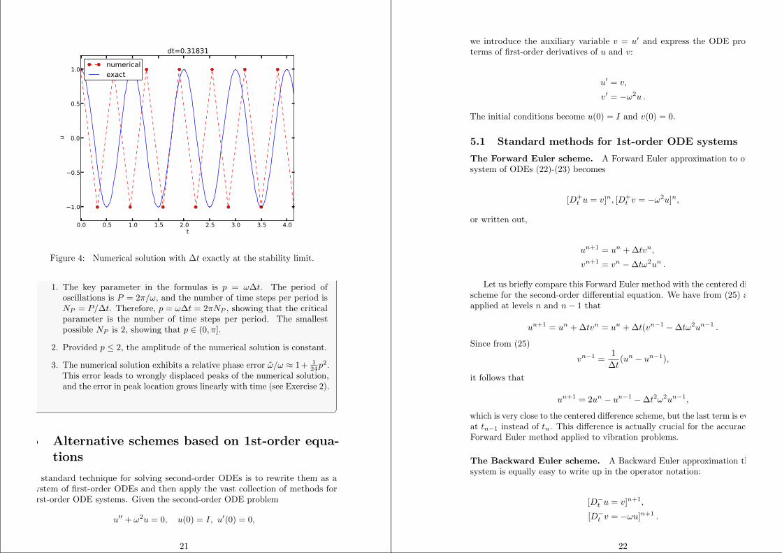
With ω = 2π, ∆t > π−1 = 0.3183098861837907 will give growing solutions.Figure 3 displays what happens when ∆t = 0.3184, which is slightly above thecritical value: ∆t = π−1 + 9.01 · 10−5.

4.5 About the accuracy at the stability limit

An interesting question is whether the stability condition ∆t < 2/ω is unfortunate,or more precisely: would it be meaningful to take larger time steps to speed

8http://www.wolframalpha.com

19

Figure 3: Growing, unstable solution because of a time step slightly beyondthe stability limit.

up computations? The answer is a clear no. At the stability limit, we havethat sin−1 ω∆t/2 = sin−1 1 = π/2, and therefore ω = π/∆t. (Note that theapproximate formula (18) is very inaccurate for this value of ∆t as it predictsω = 2.34/pi, which is a 25 percent reduction.) The corresponding period of thenumerical solution is P = 2π/ω = 2∆t, which means that there is just one timestep ∆t between a peak and a through in the numerical solution. This is theshortest possible wave that can be represented in the mesh. In other words, it isnot meaningful to use a larger time step than the stability limit.

Also, the phase error when ∆t = 2/ω is severe: Figure 4 shows a comparisonof the numerical and analytical solution with ω = 2π and ∆t = 2/ω = π−1.Already after one period, the numerical solution has a through while the exactsolution has a peak (!). The error in frequency when ∆t is at the stability limitbecomes ω − ω = ω(1− π/2) ≈ −0.57ω. The corresponding error in the periodis P − P ≈ 0.36P . The error after m periods is then 0.36mP . This error hasreach half a period when m = 1/(2 · 0.36) ≈ 1.38, which theoretically confirmsthe observations in Figure 4 that the numerical solution is a through ahead of apeak already after one and a half period.

Summary.

From the accuracy and stability analysis we can draw three importantconclusions:

20

0.0 0.5 1.0 1.5 2.0 2.5 3.0 3.5 4.0t

1.0

0.5

0.0

0.5

1.0

u

dt=0.31831

numericalexact

Figure 4: Numerical solution with ∆t exactly at the stability limit.

1. The key parameter in the formulas is p = ω∆t. The period ofoscillations is P = 2π/ω, and the number of time steps per period isNP = P/∆t. Therefore, p = ω∆t = 2πNP , showing that the criticalparameter is the number of time steps per period. The smallestpossible NP is 2, showing that p ∈ (0, π].

2. Provided p ≤ 2, the amplitude of the numerical solution is constant.

3. The numerical solution exhibits a relative phase error ω/ω ≈ 1 + 124p

2.This error leads to wrongly displaced peaks of the numerical solution,and the error in peak location grows linearly with time (see Exercise 2).

5 Alternative schemes based on 1st-order equa-tions

A standard technique for solving second-order ODEs is to rewrite them as asystem of first-order ODEs and then apply the vast collection of methods forfirst-order ODE systems. Given the second-order ODE problem

u′′ + ω2u = 0, u(0) = I, u′(0) = 0,

21

we introduce the auxiliary variable v = u′ and express the ODE problem interms of first-order derivatives of u and v:

u′ = v, (22)

v′ = −ω2u . (23)

The initial conditions become u(0) = I and v(0) = 0.

5.1 Standard methods for 1st-order ODE systems

The Forward Euler scheme. A Forward Euler approximation to our 2× 2system of ODEs (22)-(23) becomes

[D+t u = v]n, [D+

t v = −ω2u]n, (24)

or written out,

un+1 = un + ∆tvn, (25)

vn+1 = vn −∆tω2un . (26)

Let us briefly compare this Forward Euler method with the centered differencescheme for the second-order differential equation. We have from (25) and (26)applied at levels n and n− 1 that

un+1 = un + ∆tvn = un + ∆t(vn−1 −∆tω2un−1 .

Since from (25)

vn−1 =1

∆t(un − un−1),

it follows that

un+1 = 2un − un−1 −∆t2ω2un−1,

which is very close to the centered difference scheme, but the last term is evaluatedat tn−1 instead of tn. This difference is actually crucial for the accuracy of theForward Euler method applied to vibration problems.

The Backward Euler scheme. A Backward Euler approximation the ODEsystem is equally easy to write up in the operator notation:

[D−t u = v]n+1, (27)

[D−t v = −ωu]n+1 . (28)

22

This becomes a coupled system for un+1 and vn+1:

un+1 −∆tvn+1 = un, (29)

vn+1 + ∆tω2un+1 = vn . (30)

The Crank-Nicolson scheme. The Crank-Nicolson scheme takes this formin the operator notation:

[Dtu = vt]n+ 12 , (31)

[Dtv = −ωut]n+ 12 . (32)

Writing the equations out shows that is also a coupled system:

un+1 − 1

2∆tvn+1 = un +

1

2∆tvn, (33)

vn+1 +1

2∆tω2un+1 = vn − 1

2∆tω2un . (34)

Comparison of schemes. We can easily compare methods like the ones above(and many more!) with the aid of the Odespy9 package. Below is a sketch of thecode.

import odespyimport numpy as np

def f(u, t, w=1):u, v = u # u is array of length 2 holding our [u, v]return [v, -w**2*u]

def run_solvers_and_plot(solvers, timesteps_per_period=20,num_periods=1, I=1, w=2*np.pi):

P = 2*np.pi/w # duration of one perioddt = P/timesteps_per_periodNt = num_periods*timesteps_per_periodT = Nt*dtt_mesh = np.linspace(0, T, Nt+1)

legends = []for solver in solvers:

solver.set(f_kwargs={’w’: w})solver.set_initial_condition([I, 0])u, t = solver.solve(t_mesh)

There is quite some more code dealing with plots also, and we refer to the sourcefile vib_undamped_odespy.py10 for details. Observe that keyword arguments inf(u,t,w=1) can be supplied through a solver parameter f_kwargs (dictionary).

9https://github.com/hplgit/odespy10http://tinyurl.com/jvzzcfn/vib/vib undamped odespy.py

23

Specification of the Forward Euler, Backward Euler, and Crank-Nicolsonschemes is done like this:

solvers = [odespy.ForwardEuler(f),# Implicit methods must use Newton solver to convergeodespy.BackwardEuler(f, nonlinear_solver=’Newton’),odespy.CrankNicolson(f, nonlinear_solver=’Newton’),]

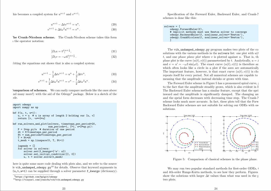
The vib_undamped_odespy.py program makes two plots of the computedsolutions with the various methods in the solvers list: one plot with u(t) versust, and one phase plane plot where v is plotted against u. That is, the phaseplane plot is the curve (u(t), v(t)) parameterized by t. Analytically, u = I cos(ωt)and v = u′ = −ωI sin(ωt). The exact curve (u(t), v(t)) is therefore an ellipse,which often looks like a circle in a plot if the axes are automatically scaled.The important feature, however, is that exact curve (u(t), v(t)) is closed andrepeats itself for every period. Not all numerical schemes are capable to do that,meaning that the amplitude instead shrinks or grows with time.

The Forward Euler scheme in Figure 5 has a pronounced spiral curve, pointingto the fact that the amplitude steadily grows, which is also evident in Figure 6.The Backward Euler scheme has a similar feature, except that the spriral goesinward and the amplitude is significantly damped. The changing amplitudeand the sprial form decreases with decreasing time step. The Crank-Nicolsonscheme looks much more accurate. In fact, these plots tell that the Forward andBackward Euler schemes are not suitable for solving our ODEs with oscillatingsolutions.

2 1 0 1 2 3u(t)

10

5

0

5

10

15

v(t

)

Time step: 0.05

ForwardEulerBackwardEulerMidpointImplicitexact

1.5 1.0 0.5 0.0 0.5 1.0 1.5 2.0u(t)

8

6

4

2

0

2

4

6

8

10

v(t

)

Time step: 0.025

ForwardEulerBackwardEulerMidpointImplicitexact

Figure 5: Comparison of classical schemes in the phase plane.

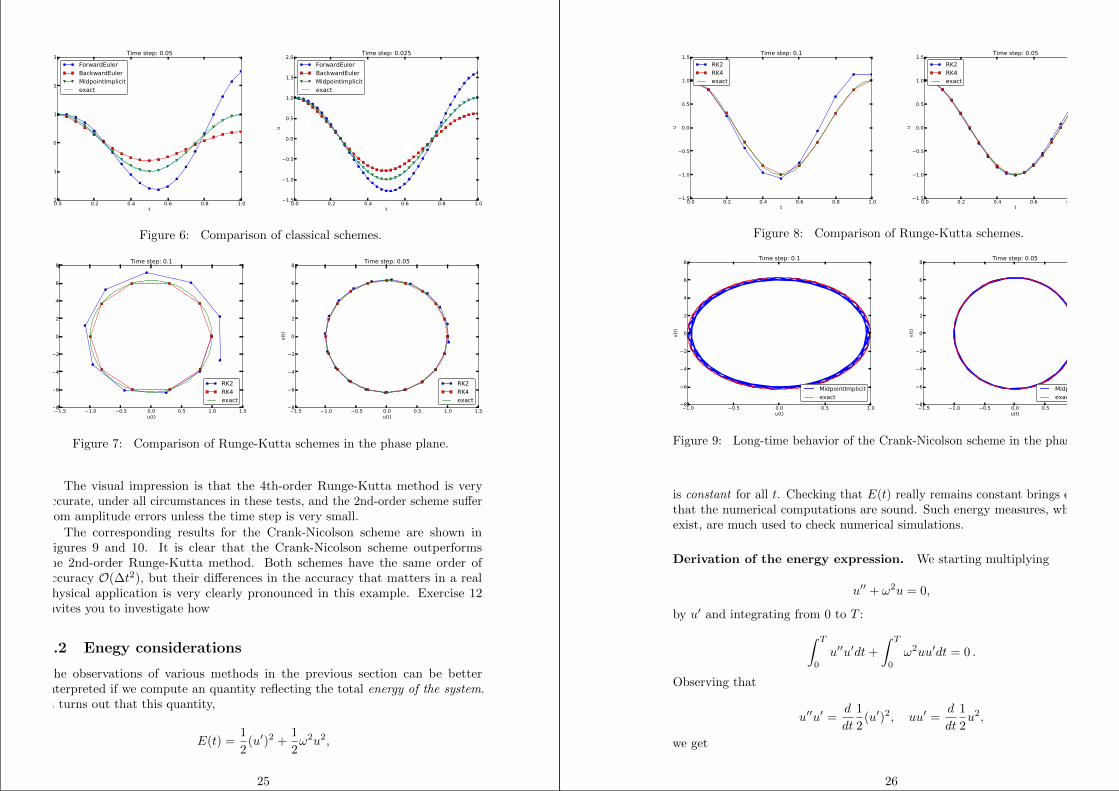
We may run two popular standard methods for first-order ODEs, the 2nd-and 4th-order Runge-Kutta methods, to see how they perform. Figures 7 and 8show the solutions with larger ∆t values than what was used in the previoustwo plots.

24

0.0 0.2 0.4 0.6 0.8 1.0t

2

1

0

1

2

3

u

Time step: 0.05

ForwardEulerBackwardEulerMidpointImplicitexact

0.0 0.2 0.4 0.6 0.8 1.0t

1.5

1.0

0.5

0.0

0.5

1.0

1.5

2.0

u

Time step: 0.025

ForwardEulerBackwardEulerMidpointImplicitexact

Figure 6: Comparison of classical schemes.

1.5 1.0 0.5 0.0 0.5 1.0 1.5u(t)

8

6

4

2

0

2

4

6

8

v(t

)

Time step: 0.1

RK2RK4exact

1.5 1.0 0.5 0.0 0.5 1.0 1.5u(t)

8

6

4

2

0

2

4

6

8

v(t

)

Time step: 0.05

RK2RK4exact

Figure 7: Comparison of Runge-Kutta schemes in the phase plane.

The visual impression is that the 4th-order Runge-Kutta method is veryaccurate, under all circumstances in these tests, and the 2nd-order scheme sufferfrom amplitude errors unless the time step is very small.

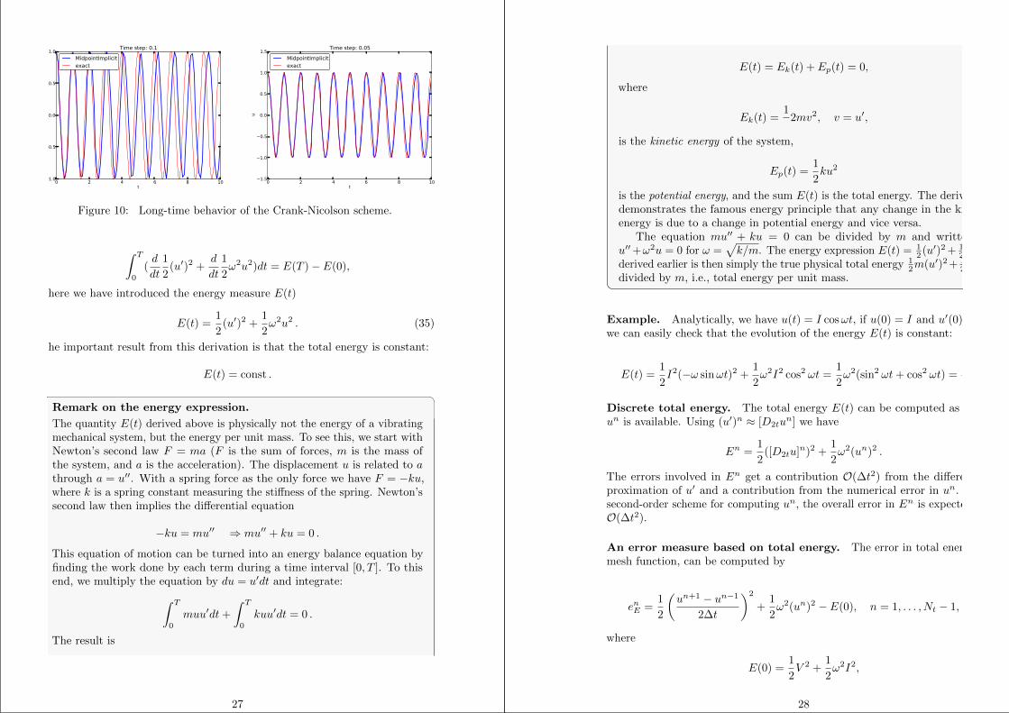
The corresponding results for the Crank-Nicolson scheme are shown inFigures 9 and 10. It is clear that the Crank-Nicolson scheme outperformsthe 2nd-order Runge-Kutta method. Both schemes have the same order ofaccuracy O(∆t2), but their differences in the accuracy that matters in a realphysical application is very clearly pronounced in this example. Exercise 12invites you to investigate how

5.2 Enegy considerations

The observations of various methods in the previous section can be betterinterpreted if we compute an quantity reflecting the total energy of the system.It turns out that this quantity,

E(t) =1

2(u′)2 +

1

2ω2u2,

25

0.0 0.2 0.4 0.6 0.8 1.0t

1.5

1.0

0.5

0.0

0.5

1.0

1.5

u

Time step: 0.1

RK2RK4exact

0.0 0.2 0.4 0.6 0.8 1.0t

1.5

1.0

0.5

0.0

0.5

1.0

1.5

u

Time step: 0.05

RK2RK4exact

Figure 8: Comparison of Runge-Kutta schemes.

1.0 0.5 0.0 0.5 1.0u(t)

8

6

4

2

0

2

4

6

8

v(t

)

Time step: 0.1

MidpointImplicitexact

1.5 1.0 0.5 0.0 0.5 1.0 1.5u(t)

8

6

4

2

0

2

4

6

8

v(t

)

Time step: 0.05

MidpointImplicitexact

Figure 9: Long-time behavior of the Crank-Nicolson scheme in the phase plane.

is constant for all t. Checking that E(t) really remains constant brings evidencethat the numerical computations are sound. Such energy measures, when theyexist, are much used to check numerical simulations.

Derivation of the energy expression. We starting multiplying

u′′ + ω2u = 0,

by u′ and integrating from 0 to T :

∫ T

0

u′′u′dt+

∫ T

0

ω2uu′dt = 0 .

Observing that

u′′u′ =d

dt

1

2(u′)2, uu′ =

d

dt

1

2u2,

we get

26

0 2 4 6 8 10t

1.0

0.5

0.0

0.5

1.0

u

Time step: 0.1

MidpointImplicitexact

0 2 4 6 8 10t

1.5

1.0

0.5

0.0

0.5

1.0

1.5

u

Time step: 0.05

MidpointImplicitexact

Figure 10: Long-time behavior of the Crank-Nicolson scheme.

∫ T

0

(d

dt

1

2(u′)2 +

d

dt

1

2ω2u2)dt = E(T )− E(0),

where we have introduced the energy measure E(t)

E(t) =1

2(u′)2 +

1

2ω2u2 . (35)

The important result from this derivation is that the total energy is constant:

E(t) = const .

Remark on the energy expression.

The quantity E(t) derived above is physically not the energy of a vibratingmechanical system, but the energy per unit mass. To see this, we start withNewton’s second law F = ma (F is the sum of forces, m is the mass ofthe system, and a is the acceleration). The displacement u is related to athrough a = u′′. With a spring force as the only force we have F = −ku,where k is a spring constant measuring the stiffness of the spring. Newton’ssecond law then implies the differential equation

−ku = mu′′ ⇒ mu′′ + ku = 0 .

This equation of motion can be turned into an energy balance equation byfinding the work done by each term during a time interval [0, T ]. To thisend, we multiply the equation by du = u′dt and integrate:

∫ T

0

muu′dt+

∫ T

0

kuu′dt = 0 .

The result is

27

E(t) = Ek(t) + Ep(t) = 0,

where

Ek(t) =1

2mv2, v = u′, (36)

is the kinetic energy of the system,

Ep(t) =1

2ku2 (37)

is the potential energy, and the sum E(t) is the total energy. The derivationdemonstrates the famous energy principle that any change in the kineticenergy is due to a change in potential energy and vice versa.

The equation mu′′ + ku = 0 can be divided by m and written asu′′+ω2u = 0 for ω =

√k/m. The energy expression E(t) = 1

2 (u′)2 + 12ω

2u2

derived earlier is then simply the true physical total energy 12m(u′)2 + 1

2k2u2

divided by m, i.e., total energy per unit mass.

Example. Analytically, we have u(t) = I cosωt, if u(0) = I and u′(0) = 0, sowe can easily check that the evolution of the energy E(t) is constant:

E(t) =1

2I2(−ω sinωt)2 +

1

2ω2I2 cos2 ωt =

1

2ω2(sin2 ωt+ cos2 ωt) =

1

2ω2 .

Discrete total energy. The total energy E(t) can be computed as soon asun is available. Using (u′)n ≈ [D2tu

n] we have

En =1

2([D2tu]n)2 +

1

2ω2(un)2 .

The errors involved in En get a contribution O(∆t2) from the difference ap-proximation of u′ and a contribution from the numerical error in un. With asecond-order scheme for computing un, the overall error in En is expected to beO(∆t2).

An error measure based on total energy. The error in total energy, as amesh function, can be computed by

enE =1

2

(un+1 − un−1

2∆t

)2

+1

2ω2(un)2 − E(0), n = 1, . . . , Nt − 1, (38)

where

E(0) =1

2V 2 +

1

2ω2I2,

28

if u(0) = I and u′(0) = V . A useful norm can be the maximum absolute valueof enE :

||enE ||`∞ = max1≤n<Nt

|enE | .

The corresponding Python implementation takes the form

# import numpy as np and compute u, tdt = t[1]-t[0]E = 0.5*((u[2:] - u[:-2])/(2*dt))**2 + 0.5*w**2*u[1:-1]**2E0 = 0.5*V**2 + 0.5**w**2*I**2e_E = E - E0e_E_norm = np.abs(e_E).max()

The convergence rates of the quantity e_E_norm can be used for verification.The value of e_E_norm is also useful for comparing schemes through their abilityto preserve energy. Below is a table demonstrating the error in total energyfor various schemes. We clearly see that the Crank-Nicolson and 4th-orderRunge-Kutta schemes are superior to the 2nd-order Runge-Kutta method andeven more superior to the Forward and Backward Euler schemes.

Method T ∆t max |enE |Forward Euler 1 0.05 1.113 · 102

Forward Euler 1 0.025 3.312 · 101

Backward Euler 1 0.05 1.683 · 101

Backward Euler 1 0.025 1.231 · 101

Runge-Kutta 2nd-order 1 0.1 8.401Runge-Kutta 2nd-order 1 0.05 9.637 · 10−1

Crank-Nicolson 1 0.05 9.389 · 10−1

Crank-Nicolson 1 0.025 2.411 · 10−1

Runge-Kutta 4th-order 1 0.1 2.387Runge-Kutta 4th-order 1 0.05 6.476 · 10−1

Crank-Nicolson 10 0.1 3.389Crank-Nicolson 10 0.05 9.389 · 10−1

Runge-Kutta 4th-order 10 0.1 3.686Runge-Kutta 4th-order 10 0.05 6.928 · 10−1

5.3 The Euler-Cromer method

While the 4th-order Runge-Kutta method and the a centered Crank-Nicolsonscheme work well for the first-order formulation of the vibration model, both wereinferior to the straightforward centered difference scheme for the second-orderequation u′′ + ω2u = 0. However, there is a similarly successful scheme availablefor the first-order system u′ = v, v′ = −ω2u, to be presented next.

29

Forward-backward discretization. The idea is to apply a Forward Eulerdiscretization to the first equation and a Backward Euler discretization to thesecond. In operator notation this is stated as

[D+t u = v]n, (39)

[D−t v = −ωu]n+1 . (40)

We can write out the formulas and collect the unknowns on the left-hand side:

un+1 = un + ∆tvn, (41)

vn+1 = vn −∆tω2un+1 . (42)

We realize that un+1 can be computed from (41) and then vn+1 from (42) usingthe recently computed value un+1 on the right-hand side.

The scheme (41)-(42) goes under several names: Forward-backward scheme,Semi-implicit Euler method11, symplectic Euler, semi-explicit Euler, Newton-Stormer-Verlet, and Euler-Cromer. We shall stick to the latter name. Since bothtime discretizations are based on first-order difference approximation, one maythink that the scheme is only of first-order, but this is not true: the use of aforward and then a backward difference make errors cancel so that the overallerror in the scheme is O(∆t2). This is explaned below.

Equivalence with the scheme for the second-order ODE. We may elim-inate the vn variable from (41)-(42). From (42) we have vn = vn−1 −∆tω2un,which can be inserted in (41) to yield

un+1 = un + ∆tvn−1 −∆t2ω2un. (43)

The vn−1 quantity can be expressed by un and un−1 using (41):

vn−1 =un − un−1

∆t,

and when this is inserted in (43) we get

un+1 = 2un − un−1 −∆t2ω2un, (44)

which is nothing but the centered scheme (7)! The previous analysis of thisscheme then also applies to the Euler-Cromer method. That is, the amplitudeis constant, given that the stability criterion is fulfilled, but there is always aphase error (18).

The initial condition u′ = 0 means u′ = v = 0. Then v0 = 0, and (41) impliesu1 = u0, while (42) says v1 = −ω2u0. This approximation, u1 = u0, correspondsto a first-order Forward Euler discretization of the initial condition u′(0) = 0:[D+

t u = 0]0. Therefore, the Euler-Cromer scheme will start out differently andnot exactly reproduce the solution of (7).

11http://en.wikipedia.org/wiki/Semi-implicit Euler method

30

5.4 The Euler-Cromer scheme on a staggered mesh

The Forward and Backward Euler schemes used in the Euler-Cromer method areboth non-symmetric, but their combination yields a symmetric method since theresulting scheme is equivalent with a centered (symmetric) difference scheme foru′′ + ω2u = 0. The symmetric nature of the Euler-Cromer scheme is much moreevident if we introduce a staggered mesh in time where u is sought at integertime points tn and v is sought at tn+1/2 between two u points. The unknowns

are then u1, v3/2, u2, v5/2, and so on. We typically use the notation un and vn+ 12

for the two unknown mesh functions.On a staggered mesh it is natural to use centered difference approximations,

expressed in operator notation as

[Dtu = v]n+ 12 , (45)

[Dtv = −ωu]n+1 . (46)

Writing out the formulas gives

un+1 = un + ∆tvn+ 12 , (47)

vn+ 32 = vn+ 1

2 −∆tω2un+1 . (48)

Of esthetic reasons one often writes these equations at the previous time level toreplace the 3

2 by 12 in the left-most term in the last equation,

un = un−1 + ∆tvn−12 , (49)

vn+ 12 = vn−

12 −∆tω2un . (50)

Such a rewrite is only mathematical cosmetics. The important thing is that thiscentered scheme has exactly the same computational structure as the forward-backward scheme. We shall use the names forward-backward Euler-Cromer andstaggered Euler-Cromer to distinguish the two schemes.

We can eliminate the v values and get back the centered scheme based onthe second-order differential equation, so all these three schemes are equivalent.However, they differ somewhat in the treatment of the initial conditions.

Suppose we have u(0) = I and u′(0) = v(0) = 0 as mathematical initialconditions. This means u0 = I and

v(0) ≈ 1

2(v−

12 + v

12 ) = 0, ⇒ v−

12 = −v 1

2 .

Using the discretized equation (50) for n = 0 yields

v12 = v−

12 −∆tω2I,

and eliminating v−12 = −v 1

2 results in v12 = − 1

2∆tω2I and

31

u1 = u0 − 1

2∆t2ω2I,

which is exactly the same equation for u1 as we had in the centered scheme basedon the second-order differential equation (and hence corresponds to a centereddifference approximation of the initial condition for u′(0)). The conclusion is thata staggered mesh is fully equivalent with that scheme, while the forward-backwardversion gives a slight deviation in the computation of u1.

We can redo the derivation of the initial conditions when u′(0) = V :

v(0) ≈ 1

2(v−

12 + v

12 ) = V, ⇒ v−

12 = 2V − v 1

2 .

Using this v−12 in

v12 = v−

12 −∆tω2I,

then gives v12 = V − 1

2∆tω2I. The general initial conditions are therefore

u0 = I, (51)

v12 = V − 1

2∆tω2I . (52)

5.5 Implementation of the scheme on a staggered mesh

The algorithm goes like this:

1. Set the initial values (51) and (52).

2. For n = 1, 2, . . .:

(a) Compute un from (49).

(b) Compute vn+ 12 from (50).

Implementation with integer indices. Translating the schemes (49) and

(50) to computer code faces the problem of how to store and access vn+ 12 ,

since arrays only allow integer indices with base 0. We must then introduce aconvention: v1+ 1

2 is stored in v[n] while v1− 12 is stored in v[n-1]. We can then

write the algorithm in Python as

def solver(I, w, dt, T):dt = float(dt)Nt = int(round(T/dt))u = zeros(Nt+1)v = zeros(Nt+1)t = linspace(0, Nt*dt, Nt+1) # mesh for ut_v = t + dt/2 # mesh for v

32

u[0] = Iv[0] = 0 - 0.5*dt*w**2*u[0]for n in range(1, Nt+1):

u[n] = u[n-1] + dt*v[n-1]v[n] = v[n-1] - dt*w**2*u[n]

return u, t, v, t_v

Note that the return u and v together with the mesh points such that thecomplete mesh function for u is described by u and t, while v and t_v representsthe mesh function for v.

Implementation with half-integer indices. Some prefer to see a closerrelationship between the code and the mathematics for the quantities withhalf-integer indices. For example, we would like to replace the updating equationfor v[n] by

v[n+half] = v[n-half] - dt*w**2*u[n]

This is easy to do if we could be sure that n+half means n and n-half meansn-1. A possible solution is to define half as a special object such that an integerplus half results in the integer, while an integer minus half equals the integerminus 1. A simple Python class may realize the half object:

class HalfInt:def __radd__(self, other):

return other

def __rsub__(self, other):return other - 1

half = HalfInt()

The __radd__ function is invoked for all expressions n+half (”right add” withself as half and other as n). Similarly, the __rsub__ function is invoked forn-half and results in n-1.

Using the half object, we can implement the algorithms in an even morereadable way:

def solver(I, w, dt, T):"""Solve u’=v, v’ = - w**2*u for t in (0,T], u(0)=I and v(0)=0,by a central finite difference method with time step dt."""dt = float(dt)Nt = int(round(T/dt))u = zeros(Nt+1)v = zeros(Nt+1)t = linspace(0, Nt*dt, Nt+1) # mesh for ut_v = t + dt/2 # mesh for v

u[0] = Iv[0+half] = 0 - 0.5*dt*w**2*u[0]for n in range(1, Nt+1):

33

print n, n+half, n-halfu[n] = u[n-1] + dt*v[n-half]v[n+half] = v[n-half] - dt*w**2*u[n]

return u, t, v, t_v

Verification of this code is easy as we can just compare the computed u

with the u produced by the solver function in vib_undamped.py (which solvesu′′ + ω2u = 0 directly). The values should coincide to machine precision sincethe two numerical methods are mathematically equivalent. We refer to the filevib_undamped_staggered.py12 for the details of a nose test that checks thisproperty.

6 Generalization: damping, nonlinear spring, andexternal excitation

We shall now generalize the simple model problem from Section 1 to include apossibly nonlinear damping term f(u′), a possibly nonlinear spring (or restoring)force s(u), and some external excitation F (t):

mu′′ + f(u′) + s(u) = F (t), u(0) = I, u′(0) = V, t ∈ (0, T ] . (53)

We have also included a possibly nonzero initial value of u′(0). The parametersm, f(u′), s(u), F (t), I, V , and T are input data.

There are two main types of damping (friction) forces: linear f(u′) = bu, orquadratic f(u′) = bu′|u′|. Spring systems often feature linear damping, whileair resistance usually gives rise to quadratic damping. Spring forces are oftenlinear: s(u) = cu, but nonlinear versions are also common, the most famous isthe gravity force on a pendulum that acts as a spring with s(u) ∼ sin(u).

6.1 A centered scheme for linear damping

Sampling (53) at a mesh point tn, replacing u′′(tn) by [DtDtu]n, and u′(tn) by[D2tu]n results in the discretization

[mDtDtu+ f(D2tu) + s(u) = F ]n, (54)

which written out means

mun+1 − 2un + un−1

∆t2+ f(

un+1 − un−1

2∆t) + s(un) = Fn, (55)

where Fn as usual means F (t) evaluated at t = tn. Solving (55) with respect tothe unknown un+1 gives a problem: the un+1 inside the f function makes theequation nonlinear unless f(u′) is a linear function, f(u′) = bu′. For now weshall assume that f is linear in u′. Then

12http://tinyurl.com/jvzzcfn/vib/vib undamped staggered.py

34

mun+1 − 2un + un−1

∆t2+ b

un+1 − un−1

2∆t+ s(un) = Fn, (56)

which gives an explicit formula for u at each new time level:

un+1 = (2mun + (b

2∆t−m)un−1 + ∆t2(Fn − s(un)))(m+

b

2∆t)−1 . (57)

For the first time step we need to discretize u′(0) = V as [D2tu = V ]0 andcombine with (57) for n = 0. The discretized initial condition leads to

u−1 = u1 − 2∆tV, (58)

which inserted in (57) for n = 0 gives an equation that can be solved for u1:

u1 = u0 + ∆t V +∆t2

2m(−bV − s(u0) + F 0) . (59)

6.2 A centered scheme for quadratic damping

When f(u′) = bu′|u′|, we get a quadratic equation for un+1 in (55). Thisequation can straightforwardly be solved, but we can also avoid the nonlinearityby performing an approximation that is within other numerical errors that wehave already committed by replacing derivatives with finite differences.

The idea is to reconsider (53) and only replace u′′ by DtDtu, giving

[mDtDtu+ bu′|u′|+ s(u) = F ]n, (60)

Here, u′|u′| is to be computed at time tn. We can introduce a geometric mean,defined by

(w2)n ≈ wn− 12wn+ 1

2 ,

for some quantity w depending on time. The error in the geometric meanapproximation is O(∆t2), the same as in the approximation u′′ ≈ DtDtu. Withw = u′ it follows that

[u′|u′|]n ≈ u′(tn +1

2)|u′(tn −

1

2)| .

The next step is to approximate u′ at tn±1/2, but here a centered difference canbe used:

u′(tn+1/2) ≈ [Dtu]n+ 12 , u′(tn−1/2) ≈ [Dtu]n−

12 . (61)

We then get

[u′|u′|]n ≈ [Dtu]n+ 12 |[Dtu]n−

12 | = un+1 − un

∆t

|un − un−1|∆t

. (62)

35

The counterpart to (55) is then

mun+1 − 2un + un−1

∆t2+ b

un+1 − un∆t

|un − un−1|∆t

+ s(un) = Fn, (63)

which is linear in un+1. Therefore, we can easily solve with respect to un+1 andachieve the explicit updating formula

un+1 =(m+ b|un − un−1|

)−1×(2mun −mun−1 + bun|un − un−1|+ ∆t2(Fn − s(un))

). (64)

In the derivation of a special equation for the first time step we run intosome trouble: inserting (58) in (64) for n = 0 results in a complicated nonlinearequation for u1. By thinking differently about the problem we can easily getaway with the nonlinearity again. We have for n = 0 that b[u′|u′|]0 = bV |V |.Using this value in (60) gives

[mDtDtu+ bV |V |+ s(u) = F ]0 . (65)

Writing this equation out and using (58) results in the special equation for thefirst time step:

u1 = u0 + ∆tV +∆t2

2m

(−bV |V | − s(u0) + F 0

). (66)

6.3 A forward-backward discretization of the quadraticdamping term

The previous section first proposed to discretize the quadratic damping term|u′|u′ using centered differences: [|D2t|D2tu]n. As this gives rise to a nonlinearityin un+1, it was instead proposed to use a geometric mean combined with centereddifferences. But there are other alternatives. To get rid of the nonlinearity in[|D2t|D2tu]n, one can think differently: apply a backward difference to |u′|, suchthat the term involves known values, and apply a forward difference to u′ tomake the term linear in the unknown un+1. With mathematics,

[β|u′|u′]n ≈ β|[D−t u]n|[D+t u]n = β

∣∣∣∣u−un−1

∆t

∣∣∣∣un+1 − un

∆t.

The forward and backward differences have both an error proportional to ∆t soone may think the discretization above leads to a first-order scheme. However, bylooking at the formulas, we realize that the forward-backward differences resultin exactly the same scheme as when we used a geometric mean and centereddifferences. Therefore, the forward-backward differences act in a symmetric wayand actually produce a second-order accurate discretization of the quadraticdamping term.

36

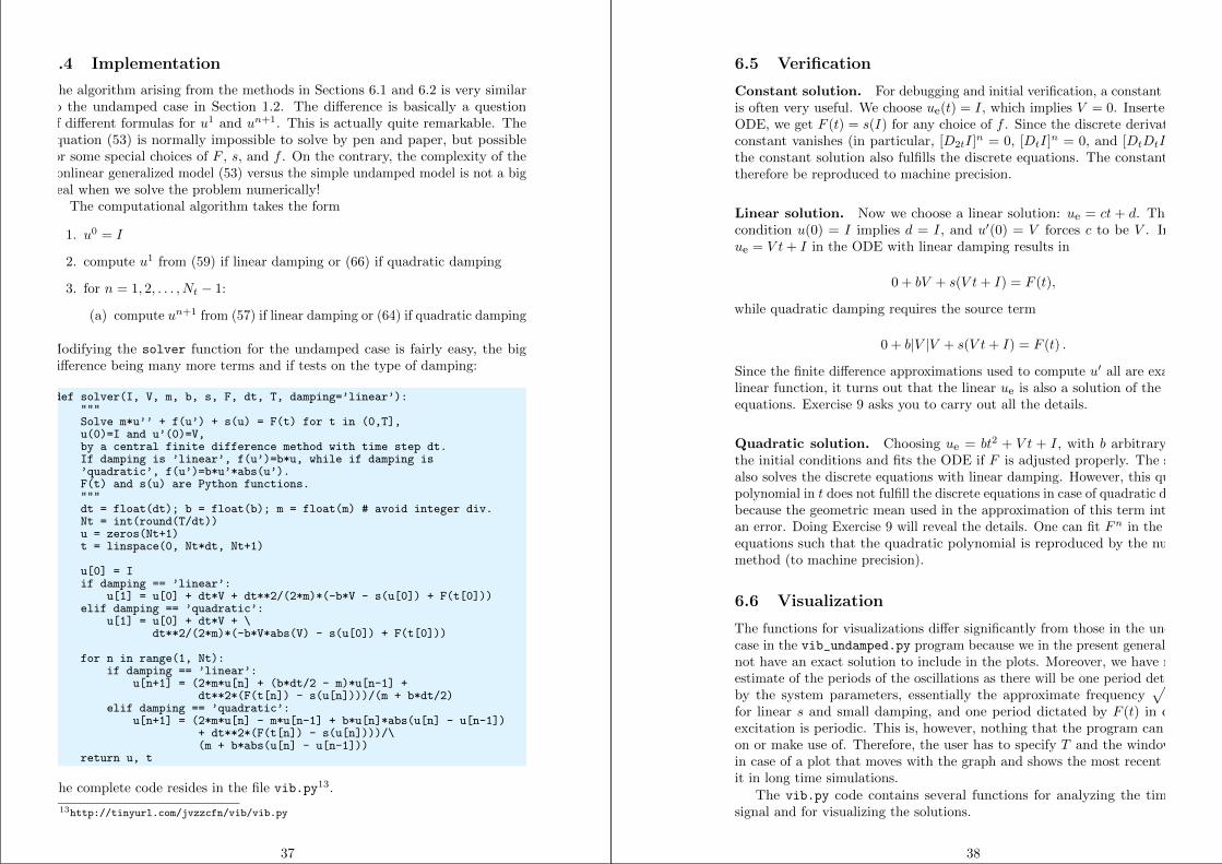
6.4 Implementation

The algorithm arising from the methods in Sections 6.1 and 6.2 is very similarto the undamped case in Section 1.2. The difference is basically a questionof different formulas for u1 and un+1. This is actually quite remarkable. Theequation (53) is normally impossible to solve by pen and paper, but possiblefor some special choices of F , s, and f . On the contrary, the complexity of thenonlinear generalized model (53) versus the simple undamped model is not a bigdeal when we solve the problem numerically!

The computational algorithm takes the form

1. u0 = I

2. compute u1 from (59) if linear damping or (66) if quadratic damping

3. for n = 1, 2, . . . , Nt − 1:

(a) compute un+1 from (57) if linear damping or (64) if quadratic damping

Modifying the solver function for the undamped case is fairly easy, the bigdifference being many more terms and if tests on the type of damping:

def solver(I, V, m, b, s, F, dt, T, damping=’linear’):"""Solve m*u’’ + f(u’) + s(u) = F(t) for t in (0,T],u(0)=I and u’(0)=V,by a central finite difference method with time step dt.If damping is ’linear’, f(u’)=b*u, while if damping is’quadratic’, f(u’)=b*u’*abs(u’).F(t) and s(u) are Python functions."""dt = float(dt); b = float(b); m = float(m) # avoid integer div.Nt = int(round(T/dt))u = zeros(Nt+1)t = linspace(0, Nt*dt, Nt+1)

u[0] = Iif damping == ’linear’:

u[1] = u[0] + dt*V + dt**2/(2*m)*(-b*V - s(u[0]) + F(t[0]))elif damping == ’quadratic’:

u[1] = u[0] + dt*V + \dt**2/(2*m)*(-b*V*abs(V) - s(u[0]) + F(t[0]))

for n in range(1, Nt):if damping == ’linear’:

u[n+1] = (2*m*u[n] + (b*dt/2 - m)*u[n-1] +dt**2*(F(t[n]) - s(u[n])))/(m + b*dt/2)

elif damping == ’quadratic’:u[n+1] = (2*m*u[n] - m*u[n-1] + b*u[n]*abs(u[n] - u[n-1])

+ dt**2*(F(t[n]) - s(u[n])))/\(m + b*abs(u[n] - u[n-1]))

return u, t

The complete code resides in the file vib.py13.

13http://tinyurl.com/jvzzcfn/vib/vib.py

37

6.5 Verification

Constant solution. For debugging and initial verification, a constant solutionis often very useful. We choose ue(t) = I, which implies V = 0. Inserted in theODE, we get F (t) = s(I) for any choice of f . Since the discrete derivative of aconstant vanishes (in particular, [D2tI]n = 0, [DtI]n = 0, and [DtDtI]n = 0),the constant solution also fulfills the discrete equations. The constant shouldtherefore be reproduced to machine precision.

Linear solution. Now we choose a linear solution: ue = ct + d. The initialcondition u(0) = I implies d = I, and u′(0) = V forces c to be V . Insertingue = V t+ I in the ODE with linear damping results in

0 + bV + s(V t+ I) = F (t),

while quadratic damping requires the source term

0 + b|V |V + s(V t+ I) = F (t) .

Since the finite difference approximations used to compute u′ all are exact for alinear function, it turns out that the linear ue is also a solution of the discreteequations. Exercise 9 asks you to carry out all the details.

Quadratic solution. Choosing ue = bt2 + V t + I, with b arbitrary, fulfillsthe initial conditions and fits the ODE if F is adjusted properly. The solutionalso solves the discrete equations with linear damping. However, this quadraticpolynomial in t does not fulfill the discrete equations in case of quadratic damping,because the geometric mean used in the approximation of this term introducesan error. Doing Exercise 9 will reveal the details. One can fit Fn in the discreteequations such that the quadratic polynomial is reproduced by the numericalmethod (to machine precision).

6.6 Visualization

The functions for visualizations differ significantly from those in the undampedcase in the vib_undamped.py program because we in the present general case donot have an exact solution to include in the plots. Moreover, we have no goodestimate of the periods of the oscillations as there will be one period determinedby the system parameters, essentially the approximate frequency

√s′(0)/m

for linear s and small damping, and one period dictated by F (t) in case theexcitation is periodic. This is, however, nothing that the program can dependon or make use of. Therefore, the user has to specify T and the window widthin case of a plot that moves with the graph and shows the most recent parts ofit in long time simulations.

The vib.py code contains several functions for analyzing the time seriessignal and for visualizing the solutions.

38

6.7 User interface

The main function has substantial changes from the vib_undamped.py codesince we need to specify the new data c, s(u), and F (t). In addition, we mustset T and the plot window width (instead of the number of periods we want tosimulate as in vib_undamped.py). To figure out whether we can use one plotfor the whole time series or if we should follow the most recent part of u, wecan use the plot_empricial_freq_and_amplitude function’s estimate of thenumber of local maxima. This number is now returned from the function andused in main to decide on the visualization technique.

def main():import argparseparser = argparse.ArgumentParser()parser.add_argument(’--I’, type=float, default=1.0)parser.add_argument(’--V’, type=float, default=0.0)parser.add_argument(’--m’, type=float, default=1.0)parser.add_argument(’--c’, type=float, default=0.0)parser.add_argument(’--s’, type=str, default=’u’)parser.add_argument(’--F’, type=str, default=’0’)parser.add_argument(’--dt’, type=float, default=0.05)parser.add_argument(’--T’, type=float, default=140)parser.add_argument(’--damping’, type=str, default=’linear’)parser.add_argument(’--window_width’, type=float, default=30)parser.add_argument(’--savefig’, action=’store_true’)a = parser.parse_args()from scitools.std import StringFunctions = StringFunction(a.s, independent_variable=’u’)F = StringFunction(a.F, independent_variable=’t’)I, V, m, c, dt, T, window_width, savefig, damping = \

a.I, a.V, a.m, a.c, a.dt, a.T, a.window_width, a.savefig, \a.damping

u, t = solver(I, V, m, c, s, F, dt, T)num_periods = empirical_freq_and_amplitude(u, t)if num_periods <= 15:

figure()visualize(u, t)

else:visualize_front(u, t, window_width, savefig)

show()

The program vib.py contains the above code snippets and can solve the modelproblem (53). As a demo of vib.py, we consider the case I = 1, V = 0, m = 1,c = 0.03, s(u) = sin(u), F (t) = 3 cos(4t), ∆t = 0.05, and T = 140. The relevantcommand to run is

Terminal> python vib.py --s ’sin(u)’ --F ’3*cos(4*t)’ --c 0.03

This results in a moving window following the function14 on the screen. Figure 11shows a part of the time series.

14http://tinyurl.com/k3sdbuv/pub/mov-vib/vib generalized dt0.05/index.html

39

0 10 20 30 40 50 60t

1.0

0.5

0.0

0.5

1.0

u

dt=0.05

Figure 11: Damped oscillator excited by a sinusoidal function.

6.8 A staggered Euler-Cromer scheme for the generalizedmodel

The model

mu′′ + f(u′) + s(u) = F (t), u(0) = I, u′(0) = V, t ∈ (0, T ], (67)

can be rewritten as a first-order ODE system

u′ = v, (68)

v′ = m−1 (F (t)− f(v)− s(u)) . (69)

It is natural to introduce a staggered mesh (see Section 5.4) and seek u atmesh points tn (the numerical value is denoted by un) and v between mesh

points at tn+1/2 (the numerical value is denoted by vn+ 12 ). A centered difference

approximation to (68)-(69) can then be written in operator notation as

[Dtu = v]n−12 , (70)

[Dtv = m−1 (F (t)− f(v)− s(u))]n . (71)

40

Written out,

un − un−1

∆t= vn−

12 , (72)

vn+ 12 − vn− 1

2

∆t= m−1 (Fn − f(vn)− s(un)) . (73)

With linear damping, f(v) = bv, we can use an arithmetic mean for f(vn):

f(vn) ≈= 12 (f(vn−

12 ) + f(vn+ 1

2 )). The system (72)-(73) can then be solved with

respect to the unknowns un and vn+ 12 :

un = un−1 + ∆tvn−12 , (74)

vn+ 12 =

(1 +

b

2m∆t

)−1(vn−

12 + ∆tm−1

(Fn − 1

2f(vn−

12 )− s(un)

)). (75)

In case of quadratic damping, f(v) = b|v|v, we can use a geometric mean:

f(vn) ≈ b|vn− 12 |vn+ 1

2 . Inserting this approximation in (72)-(73) and solving for

the unknowns un and vn+ 12 results in

un = un−1 + ∆tvn−12 , (76)

vn+ 12 = (1 +

b

m|vn− 1

2 |∆t)−1(vn−

12 + ∆tm−1 (Fn − s(un))

). (77)

The initial conditions are derived at the end of Section 5.4:

u0 = I, (78)

v12 = V − 1

2∆tω2I . (79)

7 Exercises and Problems

Problem 1: Use linear/quadratic functions for verification

Consider the ODE problem

u′′ + ω2u = f(t), u(0) = I, u′(0) = V, t ∈ (0, T ] .

Discretize this equation according to [DtDtu+ ω2u = f ]n.

a) Derive the equation for the first time step (u1).

41

b) For verification purposes, we use the method of manufactured solutions(MMS) with the choice of ue(x, t) = ct+ d. Find restrictions on c and d fromthe initial conditions. Compute the corresponding source term f by term.Show that [DtDtt]

n = 0 and use the fact that the DtDt operator is linear,[DtDt(ct+ d)]n = c[DtDtt]

n + [DtDtd]n = 0, to show that ue is also a perfectsolution of the discrete equations.

c) Use sympy to do the symbolic calculations above. Here is a sketch of theprogram vib_undamped_verify_mms.py:

import sympy as spV, t, I, w, dt = sp.symbols(’V t I w dt’) # global symbolsf = None # global variable for the source term in the ODE

def ode_source_term(u):"""Return the terms in the ODE that the source termmust balance, here u’’ + w**2*u.u is symbolic Python function of t."""return sp.diff(u(t), t, t) + w**2*u(t)

def residual_discrete_eq(u):"""Return the residual of the discrete eq. with u inserted."""R = ...return sp.simplify(R)

def residual_discrete_eq_step1(u):"""Return the residual of the discrete eq. at the firststep with u inserted."""R = ...return sp.simplify(R)

def DtDt(u, dt):"""Return 2nd-order finite difference for u_tt.u is a symbolic Python function of t."""return ...

def main(u):"""Given some chosen solution u (as a function of t, implementedas a Python function), use the method of manufactured solutionsto compute the source term f, and check if u also solvesthe discrete equations."""print ’=== Testing exact solution: %s ===’ % uprint "Initial conditions u(0)=%s, u’(0)=%s:" % \

(u(t).subs(t, 0), sp.diff(u(t), t).subs(t, 0))

# Method of manufactured solution requires fitting fglobal f # source term in the ODEf = sp.simplify(ode_lhs(u))

# Residual in discrete equations (should be 0)print ’residual step1:’, residual_discrete_eq_step1(u)print ’residual:’, residual_discrete_eq(u)

def linear():

42

main(lambda t: V*t + I)

if __name__ == ’__main__’:linear()

Fill in the various functions such that the calls in the main function works.

d) The purpose now is to choose a quadratic function ue = bt2 + ct+d as exactsolution. Extend the sympy code above with a function quadratic for fitting f

and checking if the discrete equations are fulfilled. (The function is very similarto linear.)

e) Will a polynomial of degree three fulfill the discrete equations?

f) Implement a solver function for computing the numerical solution of thisproblem.

g) Write a nose test for checking that the quadratic solution is computedto correctly (too machine precision, but the round-off errors accumulate andincrease with T ) by the solver function.

Filenames: vib_undamped_verify_mms.pdf, vib_undamped_verify_mms.py.

Exercise 2: Show linear growth of the phase with time

Consider an exact solution I cos(ωt) and an approximation I cos(ωt). Definethe phase error as time lag between the peak I in the exact solution and thecorresponding peak in the approximation after m periods of oscillations. Showthat this phase error is linear in m. Filename: vib_phase_error_growth.pdf.

Exercise 3: Improve the accuracy by adjusting the fre-quency

According to (18), the numerical frequency deviates from the exact frequency bya (dominating) amount ω3∆t2/24 > 0. Replace the w parameter in the algorithmin the solver function in vib_undamped.py by w*(1 - (1./24)*w**2*dt**2

and test how this adjustment in the numerical algorithm improves the accuracy(use ∆t = 0.1 and simulate for 80 periods, with and without adjustment of ω).

Filename: vib_adjust_w.py.

Exercise 4: See if adaptive methods improve the phase er-ror

Adaptive methods for solving ODEs aim at adjusting ∆t such that the error iswithin a user-prescribed tolerance. Implement the equation u′′ + u = 0 in theOdespy15 software. Use the example from Section ?? in [1]. Run the scheme

15https://github.com/hplgit/odespy

43

with a very low tolerance (say 10−14) and for a long time, check the number oftime points in the solver’s mesh (len(solver.t_all)), and compare the phaseerror with that produced by the simple finite difference method from Section 1.2with the same number of (equally spaced) mesh points. The question is whetherit pays off to use an adaptive solver or if equally many points with a simplemethod gives about the same accuracy. Filename: vib_undamped_adaptive.py.

Exercise 5: Use a Taylor polynomial to compute u1

As an alternative to the derivation of (8) for computing u1, one can use a Taylorpolynomial with three terms for u1:

u(t1) ≈ u(0) + u′(0)∆t+1

2u′′(0)∆t2

With u′′ = −ω2u and u′(0) = 0, show that this method also leads to (8).Generalize the condition on u′(0) to be u′(0) = V and compute u1 in this casewith both methods. Filename: vib_first_step.pdf.

Exercise 6: Find the minimal resolution of an oscillatoryfunction

Sketch the function on a given mesh which has the highest possible frequency.That is, this oscillatory ”cos-like” function has its maxima and minima atevery two grid points. Find an expression for the frequency of this function,and use the result to find the largest relevant value of ω∆t when ω is thefrequency of an oscillating function and ∆t is the mesh spacing. Filename:vib_largest_wdt.pdf.

Exercise 7: Visualize the accuracy of finite differences fora cosine function

We introduce the error fraction

E =[DtDtu]n

u′′(tn)

to measure the error in the finite difference approximation DtDtu to u′′. ComputeE for the specific choice of a cosine/sine function of the form u = exp (iωt) andshow that

E =

(2

ω∆t

)2

sin2(ω∆t

2) .

Plot E as a function of p = ω∆t. The relevant values of p are [0, π] (see Exercise 6for why p > π does not make sense). The deviation of the curve from unity visu-alizes the error in the approximation. Also expand E as a Taylor polynomial in pup to fourth degree (use, e.g., sympy). Filename: vib_plot_fd_exp_error.py.

44

Exercise 8: Verify convergence rates of the error in energy

We consider the ODE problem u′′ + ω2u = 0, u(0) = I, u′(0) = V , for t ∈ (0, T ].The total energy of the solution E(t) = 1

2 (u′)2 + 12ω

2u2 should stay constant.The error in energy can be computed as explained in Section 5.2.

Make a nose test in a file test_error_conv.py, where code from vib_undamped.py

is imported, but the convergence_rates and test_convergence_rates func-tions are copied and modified to also incorporate computations of the error inenergy and the convergence rate of this error. The expected rate is 2. Filename:test_error_conv.py.

Exercise 9: Use linear/quadratic functions for verification

This exercise is a generalization of Problem 1 to the extended model problem(53) where the damping term is either linear or quadratic. Solve the varioussubproblems and see how the results and problem settings change with thegeneralized ODE in case of linear or quadratic damping. By modifying thecode from Problem 1, sympy will do most of the work required to analyze thegeneralized problem. Filename: vib_verify_mms.py.

Exercise 10: Use an exact discrete solution for verification

Write a nose test function in a separate file that employs the exact discretesolution (19) to verify the implementation of the solver function in the filevib_undamped.py. Just import solver and make functions for the exact discretesolution and the nose test. Filename: vib_verify_discrete_omega.py.

Exercise 11: Use analytical solution for convergence ratetests

The purpose of this exercise is to perform convergence tests of the problem(53) when s(u) = ω2u and F (t) = A sinφt. Find the complete analyticalsolution to the problem in this case (most textbooks on mechanics list thevarious elements you need to write down the exact solution). Modify theconvergence_rate function from the vib_undamped.py program to performexperiments with the extended model. Verify that the error is of order ∆t2.Filename: vib_conv_rate.py.

Exercise 12: Investigate the amplitude errors of many solvers

Use the program vib_undamped_odespy.py from Section 5.1 and the ampli-tude estimation from the amplitudes function in the vib_undamped.py file(see Section 3.4) to investigate how well famous methods for 1st-order ODEscan preserve the amplitude of u in undamped oscillations. Test, for example,the 3rd- and 4th-order Runge-Kutta methods (RK3, RK4), the Crank-Nicolsonmethod (CrankNicolson), the 2nd- and 3rd-order Adams-Bashforth methods

45

(AdamsBashforth2, AdamsBashforth3), and a 2nd-order Backwards scheme(Backward2Step). The relevant governing equations are listed in Section 22.Filename: vib_amplitude_errors.py.

Exercise 13: Minimize memory usage of a vibration solver

The program vib.py16 store the complete solution u0, u1, . . . , uNt in memory,which is convenient for later plotting. Make a memory minimizing version ofthis program where only the last three un+1, un, and un−1 values are storedin memory. Write each computed (tn+1, u

n+1) pair to file. Visualize the datain the file (a cool solution is to read one line at a time and plot the u valueusing the line-by-line plotter in the visualize_front_ascii function - thistechnique makes it trivial to visualize very long time simulations). Filename:vib_memsave.py.

Exercise 14: Implement the solver via classes

Reimplement the vib.py program using a class Problem to hold all the physicalparameters of the problem, a class Solver to hold the numerical parameters andcompute the solution, and a class Visualizer to display the solution.

Hint. Use the ideas and examples from Section ?? and ?? in [1]. Morespecifically, make a superclass Problem for holding the scalar physical parametersof a problem and let subclasses implement the s(u) and F (t) functions as methods.Try to call up as much existing functionality in vib.py as possible.

Filename: vib_class.py.

Exercise 15: Show equivalence between schemes

Show that the schemes from Sections 1.2, 5.3, and 5.4 are all equivalent. Filename:vib_scheme_equivalence.pdf.

Exercise 16: Interpret [DtDtu]n as a forward-backward dif-

ference

Show that the difference [DtDtu]n is equal to [D+t D−t u]n and D−t D

+t u]n. That

is, instead of applying a centered difference twice one can alternatively apply amixture forward and backward differences. Filename: vib_DtDt_fw_bw.pdf.

Exercise 17: Use the forward-backward scheme with quadraticdamping

We consider the generalized model with quadratic damping, expressed as asystem of two first-order equations as in Section 6.8:

16http://tinyurl.com/jvzzcfn/vib/vib.py

46

u′ = v,

v′ =1

m(F (t)− β|v|v − s(u)) .

However, contrary to what is done in Section 6.8, we want to apply the idea ofthe forward-backward discretization in Section 5.3. Express the idea in operatornotation and write out the scheme. Unfortunately, the backward difference forthe v equation creates a nonlinearity |vn+1|vn. To linearize this nonlinearity, usethe known value vn inside the absolute value factor, i.e., |vn+1|vn ≈ |vn|vn+1.Show that the resulting scheme is equivalent to the one in Section 6.8 for sometime level n ≥ 1.

What we learn from this exercise is that the first-order differences and thelinearization trick play together in ”the right way” such that the scheme is asgood as when we (in Section 6.8) carefully apply centered differences and ageometric mean on a staggered mesh to achieve second-order accuracy. There isa difference in the handling of the initial conditions, though, as explained at theend of Section 5.3. Filename: vib_gen_bwdamping.pdf.

Exercise 18: Use a backward difference for the dampingterm

As an alternative to discretizing the damping terms βu′ and β|u′|u′ by centereddifferences, we may apply backward differences:

[u′]n ≈ [D−t u]n,

[|u′|u′]n ≈ [|D−t u|D−t u]n = |[D−t u]n|[D−t u]n .

The advantage of the backward difference is that the damping term is evaluatedusing known values un and un−1 only. Extend the vib.py17 code with a schemebased on using backward differences in the damping terms. Add statementsto compare the original approach with centered difference and the new idealaunched in this exercise. Perform numerical experiments to investigate howmuch accuracy that is lost by using the backward differences.

Filename: vib_gen_bwdamping.pdf.

References

[1] H. P. Langtangen. Introduction to computing with finite difference methods.Web document, Simula Research Laboratory and University of Oslo, 2013.

17http://tinyurl.com/jvzzcfn/vib/vib.py

47

Index

argparse (Python module), 39ArgumentParser (Python class), 39averaging

geometric, 35

centered difference, 5

energy principle, 25error

global, 18

finite differencescentered, 5

forced vibrations, 34forward-backward Euler-Cromer scheme,

29frequency (of oscillations), 4

geometric mean, 35

Hz (unit), 4

making movies, 12mechanical energy, 25mechanical vibrations, 4mesh

finite differences, 4mesh function, 4

nonlinear restoring force, 34nonlinear spring, 34

oscillations, 4

period (of oscillations), 4

stability criterion, 19staggered Euler-Cromer scheme, 31staggered mesh, 31

vibration ODE, 4

48